Embed Size (px)
Citation preview
A1 2011 1 / 1
A1 Time-Frequency Analysis
David Murray
[email protected]/∼dwm/Courses/2TF
Hilary 2011
A1 2011 2 / 1
Course Contents
1 From Signals to Complex Fourier Series
2 From Complex Fourier Series to the Fourier Transform
3 Convolution. The impulse response and transfer functions
4 Sampling, Aliasing
5 Power & Energy Spectra, Autocorrelation, and Spectral Densities
6 Random Processes and Signals
7 Discrete Fourier Transforms

A1 2011 3 / 1
Discrete Methods
So far in this course, we have dealt with analytical methods only.
In this lecture we will consider computational methods applicablewhen the signal is available at discrete values of a parameter n,rather than at continuous values t .
Discrete Convolution — unsurprisingDiscrete Fourier Transform — v surprising
In practice, it is likely that the values x [n] will have been obtainedby sampling a continuous signal.If the signal is not band-limited, any results obtained will besubject to aliasing.
However, our concern here is not whether the discrete signal is fitfor purpose.We assume that aliasing is not an issue.
A1 2011 4 / 1
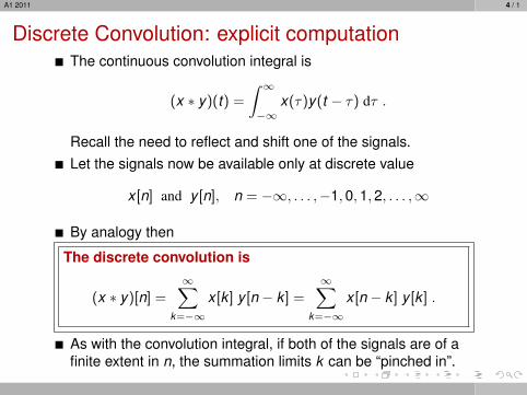
Discrete Convolution: explicit computationThe continuous convolution integral is
(x ∗ y)(t) =
∫ ∞−∞
x(τ)y(t − τ) dτ .
Recall the need to reflect and shift one of the signals.Let the signals now be available only at discrete value
x [n] and y [n], n = −∞, . . . ,−1,0,1,2, . . . ,∞
By analogy then
The discrete convolution is
(x ∗ y)[n] =∞∑
k=−∞
x [k ] y [n − k ] =∞∑
k=−∞
x [n − k ] y [k ] .
As with the convolution integral, if both of the signals are of afinite extent in n, the summation limits k can be “pinched in”.
A1 2011 5 / 1
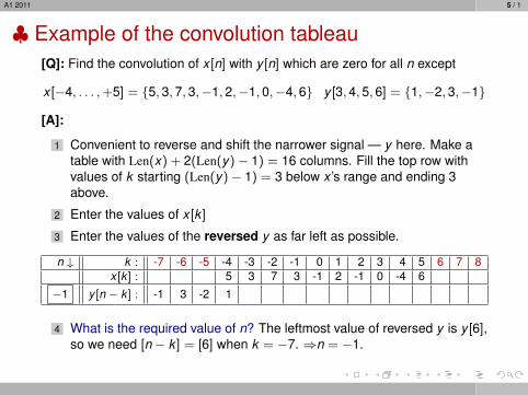
♣ Example of the convolution tableau[Q]: Find the convolution of x [n] with y [n] which are zero for all n except
x [−4, . . . ,+5] = {5, 3, 7, 3,−1, 2,−1, 0,−4, 6} y [3, 4, 5, 6] = {1,−2, 3,−1}
[A]:
1 Convenient to reverse and shift the narrower signal — y here. Make atable with Len(x) + 2(Len(y)− 1) = 16 columns. Fill the top row withvalues of k starting (Len(y)− 1) = 3 below x ’s range and ending 3above.
2 Enter the values of x [k ]
3 Enter the values of the reversed y as far left as possible.
n ↓ k : -7 -6 -5 -4 -3 -2 -1 0 1 2 3 4 5 6 7 8x [k ] : 5 3 7 3 -1 2 -1 0 -4 6
−1 y [n − k ] : -1 3 -2 1
4 What is the required value of n? The leftmost value of reversed y is y [6],so we need [n − k ] = [6] when k = −7. ⇒n = −1.

A1 2011 6 / 1
♣ Example of the convolution tableau
[A]: ctd ...
5 Fill in tableau until reversed y is as far right as possiblen ↓ k : -7 -6 -5 -4 -3 -2 -1 0 1 2 3 4 5 6 7 8 x ∗ y [n]
x [k ] : 5 3 7 3 -1 2 -1 0 -4 6−1 y [n − k ] : -1 3 -2 1 5
0 y [n − k ] : -1 3 -2 1 -71 y [n − k ] : -1 3 -2 1 162 y [n − k ] : -1 3 -2 1 -73 y [n − k ] : -1 3 -2 1 114 y [n − k ] : -1 3 -2 1 65 y [n − k ] : -1 3 -2 1 -116 y [n − k ] : -1 3 -2 1 97 y [n − k ] : -1 3 -2 1 -98 y [n − k ] : -1 3 -2 1 159 y [n − k ] : -1 3 -2 1 -24
10 y [n − k ] : -1 3 -2 1 2211 y [n − k ] : -1 3 -2 1 -6
6 Find the sum of products ...
A1 2011 7 / 1
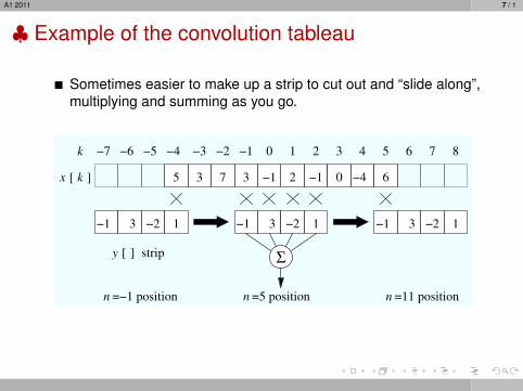
♣ Example of the convolution tableau
Sometimes easier to make up a strip to cut out and “slide along”,multiplying and summing as you go.
−1 3 −2 1 −1 3 −2 1−1 3 −2 1
=−1 positionn =5 positionn =11 positionn
−7 −6 −5 −4 −3 −2 −1 0 1 2 3 4 5 6 8
5 3
7
37 −1 2 −1 0 −4 6[ ]k
k
x
[ ] stripyΣ
A1 2011 8 / 1
Using Matlab
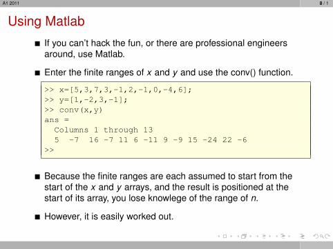
If you can’t hack the fun, or there are professional engineersaround, use Matlab.
Enter the finite ranges of x and y and use the conv() function.
>> x=[5,3,7,3,-1,2,-1,0,-4,6];>> y=[1,-2,3,-1];>> conv(x,y)ans =
Columns 1 through 135 -7 16 -7 11 6 -11 9 -9 15 -24 22 -6
>>
Because the finite ranges are each assumed to start from thestart of the x and y arrays, and the result is positioned at thestart of its array, you lose knowlege of the range of n.
However, it is easily worked out.
A1 2011 9 / 1
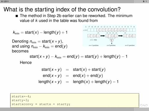
What is the starting index of the convolution?The method in Step 2b earlier can be reworked. The minimumvalue of k used in the table was found from
kmin = start(x)− length(y) + 1
Denoting nmin = start(x ∗ y),and using nmin − kmin = end(y)becomes
−1 3 −2 1 −1 3 −2 1−1 3 −2 1
=−1 positionn =5 positionn =11 positionn
−7 −6 −5 −4 −3 −2 −1 0 1 2 3 4 5 6 8
5 3
7
37 −1 2 −1 0 −4 6[ ]k
k
x
[ ] stripyΣ
start(x ∗ y)− kmin = end(y) = start(y) + length(y)− 1Hence
start(x ∗ y) = start(x) + start(y)
end(x ∗ y) = end(x) + end(y)
length(x ∗ y) = length(x) + length(y)− 1
startx=-4;starty=3;startxconvy = startx + starty;
A1 2011 10 / 1
Comment
There is nothing remarkable about discrete convolution.
Its advantage is that all the calculation occurs in the nativedomain, but its disadvantage is that if the signals x and y havelengths N and M, then the calculation takes O(NM) time.
We now turn to discuss a process which is extraordinary.
It is the Discrete Fourier Transform (DFT) which in turn willimpact on the way we could perform convolution.
This bit is hard

A1 2011 11 / 1
The Discrete Fourier Transform
In Lecture 4, we looked at the process of sampling, anddiscovered how the Fourier transform of the sampled signaldiffered from that of the original.
One notable aspect of sampling in the time domain was that thefrequency spectrum remain continuous in ω.Although the sampled time signal was ideal for representation ina computer, the frequency spectrum was not.
Question: How could sampled signals in the time domain beapproximated as sampled spectra in the frequency domain,allowing both sides to be represented in a computer?
Using the Discrete Fourier Transform ...
A1 2011 12 / 1
The Discrete Fourier Transform
We shall see that, as an abstract piece of maths, the DiscreteFourier Transform is exact (ie, it is invertible).
However as a consequence of what we noted just above, theDFT is not an exact representation of the FT.
With that caveat:the DFT can be made a very good approximation to the FT;
there is a method of computing it in O(N ln N) time using the FastFourier Transform;
it opens up methods of fast convolution and correlation; and
it opens up the full gamut of time and frequency domain analysis tocomputing.
A1 2011 13 / 1
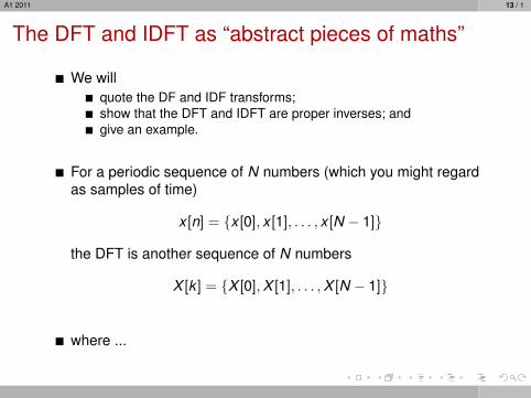
The DFT and IDFT as “abstract pieces of maths”
We willquote the DF and IDF transforms;show that the DFT and IDFT are proper inverses; andgive an example.
For a periodic sequence of N numbers (which you might regardas samples of time)
x [n] = {x [0], x [1], . . . , x [N − 1]}
the DFT is another sequence of N numbers
X [k ] = {X [0],X [1], . . . ,X [N − 1]}
where ...
A1 2011 14 / 1
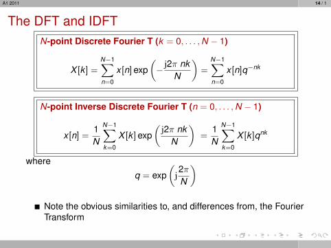
The DFT and IDFTN-point Discrete Fourier T (k = 0, . . . ,N − 1)
X [k ] =N−1∑n=0
x [n] exp(− j2π nk
N
)=
N−1∑n=0
x [n]q−nk
N-point Inverse Discrete Fourier T (n = 0, . . . ,N − 1)
x [n] =1N
N−1∑k=0
X [k ] exp(
j2π nkN
)=
1N
N−1∑k=0
X [k ]qnk
where
q = exp(
j2πN
)
Note the obvious similarities to, and differences from, the FourierTransform
A1 2011 15 / 1
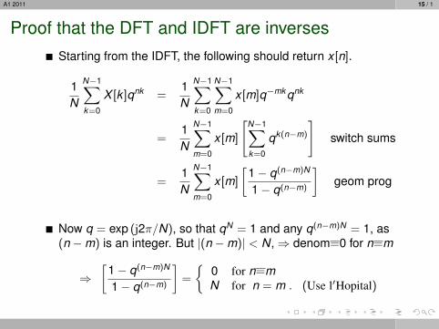
Proof that the DFT and IDFT are inversesStarting from the IDFT, the following should return x [n].
1N
N−1∑k=0
X [k ]qnk =1N
N−1∑k=0
N−1∑m=0
x [m]q−mk qnk
=1N
N−1∑m=0
x [m]
[N−1∑k=0
qk(n−m)
]switch sums
=1N
N−1∑m=0
x [m]
[1− q(n−m)N
1− q(n−m)
]geom prog
Now q = exp (j2π/N), so that qN = 1 and any q(n−m)N = 1, as(n −m) is an integer. But |(n −m)| < N,⇒ denom=0 for n=m
⇒[
1− q(n−m)N
1− q(n−m)
]=
{0 for n=mN for n = m . (Use l′Hopital)
A1 2011 16 / 1
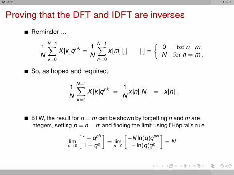
Proving that the DFT and IDFT are inverses
Reminder ...
1N
N−1∑k=0
X [k ]qnk =1N
N−1∑m=0
x [m] [·] [·] =
{0 for n=mN for n = m .
So, as hoped and required,
1N
N−1∑k=0
X [k ]qnk =1N
x [n] N = x [n] .
BTW, the result for n = m can be shown by forgetting n and m areintegers, setting p = n −m and finding the limit using l’Hôpital’s rule
limp→0
[1− qpN
1− qp
]= lim
p→0
[−N ln(q)qpN
− ln(q)qp
]= N .
A1 2011 17 / 1
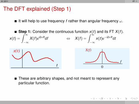
The DFT explained (Step 1)
It will help to use frequency f rather than angular frequency ω.
Step 1: Consider the continuous function x(t) and its FT X (f ).
x(t) =
∫ ∞−∞
X (f )ei2πft df ⇔ X (f ) =
∫ ∞−∞
x(t)e−i2πft dt
x(t)
tf
0
X(f)
These are arbitrary shapes, and not meant to represent anyparticular function.
A1 2011 18 / 1
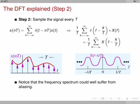
The DFT explained (Step 2)
Step 2: Sample the signal every T
x(nT ) =∞∑
n=−∞δ(t − nT )x(t) ⇔ 1
T
∞∑k=−∞
δ
(f − k
T
)∗ X (f )
=1T
∞∑k=−∞
X(
f − kT
)
t
Tx(nT)
1/T
f
−1/T 0
X(f−k/T)
Notice that the frequency spectrum could well suffer fromaliasing.

A1 2011 19 / 1
The DFT explained (Step 3)Step 3: Now isolate a run of N samples by multiplying in the timedomain by a window function w(t) — eg a tophat running from−T/2 to (N − 1)T + T/2. Defining T0 = NT , the window runsfrom −T/2 to T0 − T/2, as shown in the Figure.
The FT [w(t)] = W (f ) is a sinc function, which is phase shifted(Lecture 2).
w(t) = ⇔ W (f ) =
Π
(t − (T0 − T/2)
T0
)exp(i2πf (T0 − T/2)T0sinc(fT0)
−T/2 T0−T/2
t
w(t)
f
|W(f)|
0
Multiply Convolve
A1 2011 20 / 1
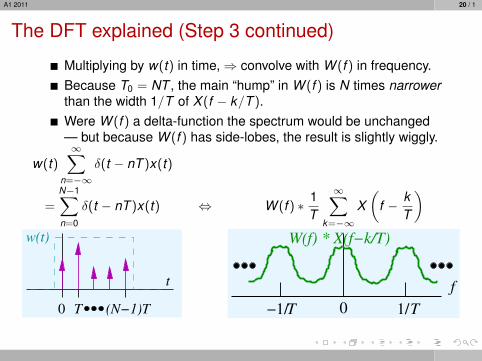
The DFT explained (Step 3 continued)
Multiplying by w(t) in time,⇒ convolve with W (f ) in frequency.Because T0 = NT , the main “hump” in W (f ) is N times narrowerthan the width 1/T of X (f − k/T ).Were W (f ) a delta-function the spectrum would be unchanged— but because W (f ) has side-lobes, the result is slightly wiggly.
w(t)∞∑
n=−∞δ(t − nT )x(t)
=N−1∑n=0
δ(t − nT )x(t) ⇔ W (f ) ∗ 1T
∞∑k=−∞
X(
f − kT
)
t
w(t)
0 T (N−1)T 1/T
f
−1/T 0
W(f) * X(f−k/T)
A1 2011 21 / 1
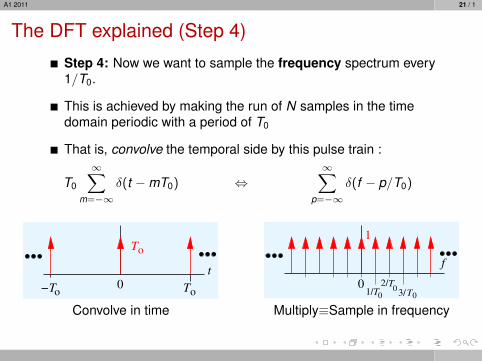
The DFT explained (Step 4)
Step 4: Now we want to sample the frequency spectrum every1/T0.
This is achieved by making the run of N samples in the timedomain periodic with a period of T0
That is, convolve the temporal side by this pulse train :
T0
∞∑m=−∞
δ(t −mT0) ⇔∞∑
p=−∞δ(f − p/T0)
0
To
To o−T
t
1/T0
2/T03/T0
0
1
f
Convolve in time Multiply≡Sample in frequency
A1 2011 22 / 1
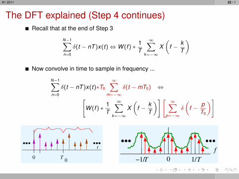
The DFT explained (Step 4 continues)Recall that at the end of Step 3
N−1∑n=0
δ(t − nT )x(t)⇔ W (f ) ∗ 1T
∞∑k=−∞
X(
f − kT
)
Now convolve in time to sample in frequency ...
N−1∑n=0
δ(t − nT )x(t)∗T0
∞∑m=−∞
δ(t −mT0) ⇔[W (f ) ∗ 1
T
∞∑k=−∞
X(
f − kT
)][ ∞∑p=−∞
δ
(f − p
T0
)]
0
t
T0 1/T
f
−1/T 0
A1 2011 23 / 1
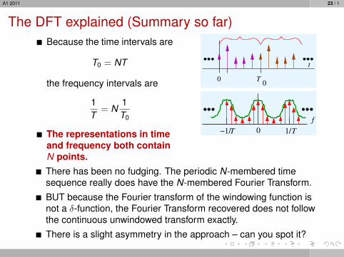
The DFT explained (Summary so far)Because the time intervals are
T0 = NT
the frequency intervals are
1T
= N1T0
The representations in timeand frequency both containN points.
0
t
T0
1/T
f
−1/T 0
There has been no fudging. The periodic N-membered timesequence really does have the N-membered Fourier Transform.BUT because the Fourier transform of the windowing function isnot a δ-function, the Fourier Transform recovered does not followthe continuous unwindowed transform exactly.There is a slight asymmetry in the approach – can you spot it?
A1 2011 24 / 1
Showing that the two N-vectors are DFTs
We now knowthe DFT and IDFT are inversesand thatthe FT of a repeated N−sampled temporal sequence is a repeatedN-sampled frequency spectrum which approximates the FT of theoriginal unsampled temporal signal.
But we have not shown that the frequency N-sample is the DFTof the temporal N-sample.
A1 2011 25 / 1
Showing that the two N-vectors are DFTs
The temporal function at the end of Step 4 was
N−1∑n=0
δ(t − nT )x(t) ∗ T0
∞∑m=−∞
δ(t −mT0)
= T0
∞∑m=−∞
N−1∑n=0
x(t)δ(t − nT ) ∗ δ(t −mT0)
= T0
∞∑m=−∞
N−1∑n=0
∫ ∞−∞
x(τ)δ(τ − nT )δ(t − τ −mT0)dτ
= T0
∞∑m=−∞
N−1∑n=0
x(nT )δ(t − nT −mT0)
Counter m makes this is a periodic function with ω0 = 2π/T0.
A1 2011 26 / 1
Showing that the two N-vectors are DFTs
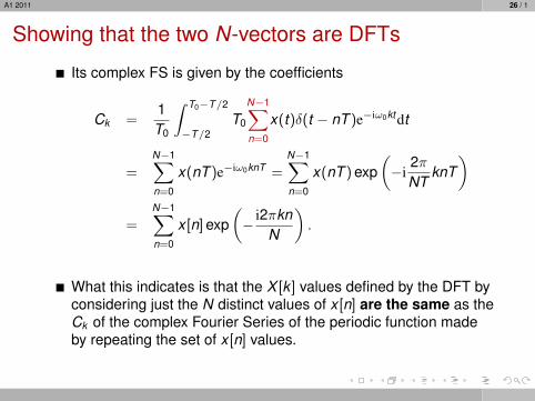
Its complex FS is given by the coefficients
Ck =1T0
∫ T0−T/2
−T/2T0
N−1∑n=0
x(t)δ(t − nT )e−iω0kt dt
=N−1∑n=0
x(nT )e−iω0knT =N−1∑n=0
x(nT ) exp(−i
2πNT
knT)
=N−1∑n=0
x [n] exp(− i2πkn
N
).
What this indicates is that the X [k ] values defined by the DFT byconsidering just the N distinct values of x [n] are the same as theCk of the complex Fourier Series of the periodic function madeby repeating the set of x [n] values.
A1 2011 27 / 1
Showing that the two N-vectors are DFTs
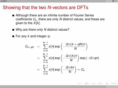
Although there are an infinite number of Fourier Seriescoefficients Ck , there are only N distinct values, and these aregiven to the X [k ].
Why are there only N distinct values?
For any k and integer q:
Ck+qN =N−1∑n=0
x [n] exp(− i2π(k + qN)n
N
)
=N−1∑n=0
x [n] exp(− i2π(k)n
N
)exp (−i2πqn)
=N−1∑n=0
x [n] exp(− i2πkn
N
)= Ck
A1 2011 28 / 1
Showing that the two N-vectors are DFTs
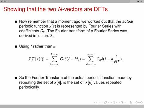
Now remember that a moment ago we worked out that the actualperiodic function x(t) is represented by Fourier Series withcoefficients Ck . The Fourier transform of a Fourier Series wasderived in lecture 3.
Using f rather than ω
FT [x(t)] =k=∞∑
k=−∞
Ckδ(f − kf0) =k=∞∑
k=−∞
Ckδ(f − k1
NT) .
So the Fourier Transform of the actual periodic function made byrepeating the set of x [n], is the set of X [k ] values repeatedperiodically.

A1 2011 29 / 1
In other words ...
The DFT and IDFT together supply a convenient short cut fortransforming between the two distinct sets of coefficients in thetime domain and frequency domain.
Notice that they are NOT formally indentical to the FourierTransform and Inverse Fourier Transform.
The motivation for all the above was to find a way of representinga sampled time signal with a sampled frequency spectrum, sothat both could be represented in a form suitable for digitalcomputation.
Note that the method did not “magic away” aliasing, and that carewould have to be taken to band limit the input to some fm and tosample at a rate above 2fm.
Also note that the step of windowing the samples in time causedchanges in the frequency spectrum.
A1 2011 30 / 1
Computing the DFT and IDFT with the Fast FourierTransform
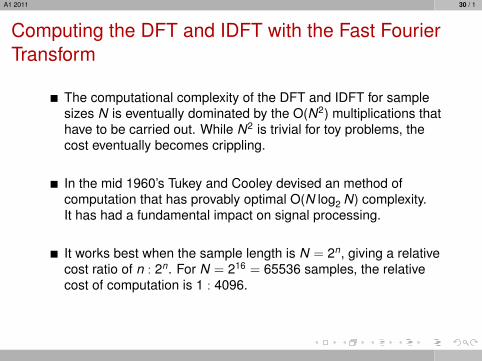
The computational complexity of the DFT and IDFT for samplesizes N is eventually dominated by the O(N2) multiplications thathave to be carried out. While N2 is trivial for toy problems, thecost eventually becomes crippling.
In the mid 1960’s Tukey and Cooley devised an method ofcomputation that has provably optimal O(N log2 N) complexity.It has had a fundamental impact on signal processing.
It works best when the sample length is N = 2n, giving a relativecost ratio of n : 2n. For N = 216 = 65536 samples, the relativecost of computation is 1 : 4096.

A1 2011 31 / 1
Properties of DFTs
Property Sampled Time Sampled Frequency CommentDomain nT Domain (k/NT )
Linearity ax [n] + by [n] aX [k ] + bY [k ] Obvious & important
Real Function Real x [n] X [−k ] = X∗[k ] Simplifies computation
Odd Function Even x [n] X [−k ] = X [k ] of transforms by
Even Function Odd x [n] X [−k ] = −X [k ] missing out terms
Duality/Symmetry (1/N)X [n] x [−k ]Time reversal x [−n] X∗[k ] x(t) real only
Time shift x [n − i] exp(− i2πmi
N
)X [k ]
Frequency shift exp(
i2πnmN
)x [n] X [k −m] Modulation
A1 2011 32 / 1
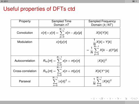
Useful properties of DFTs ctd
Property Sampled Time Sampled FrequencyDomain nT Domain (k/NT )
Convolution x [n] ∗ y [n] =N−1∑p=0
x [n − p]y [p] X [k ]Y [k ]
Modulation x [n]y [n]1N
X [k ] ∗ Y [k ]
=1N
N−1∑p=0
X [k − p]Y [p]
Autocorrelation Rxx [m] =
N−1∑n=0
x [n + m]x [n] |X [k ]|2
Cross-correlation Rxy [m] =
N−1∑n=0
x [n + m]y [n] X [k ]Y∗[k ]
ParsevalN−1∑n=0
|x [n]|2 =1N
N−1∑n=0
|X [k ]|2
A1 2011 33 / 1
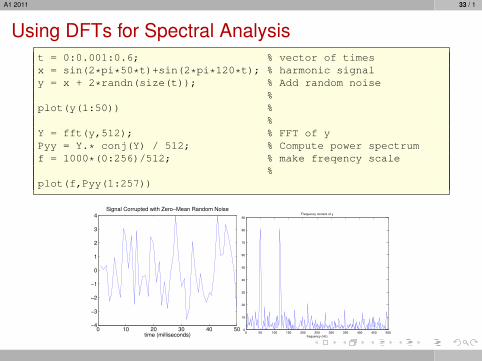
Using DFTs for Spectral Analysist = 0:0.001:0.6; % vector of timesx = sin(2*pi*50*t)+sin(2*pi*120*t); % harmonic signaly = x + 2*randn(size(t)); % Add random noise
%plot(y(1:50)) %
%Y = fft(y,512); % FFT of yPyy = Y.* conj(Y) / 512; % Compute power spectrumf = 1000*(0:256)/512; % make freqency scale
%plot(f,Pyy(1:257))
0 10 20 30 40 50−4
−3
−2
−1
0
1
2
3
4Signal Corrupted with Zero−Mean Random Noise
time (milliseconds)0 50 100 150 200 250 300 350 400 450 500
0
10
20
30
40
50
60
70
80
90Frequency content of y
frequency (Hz)
A1 2011 34 / 1
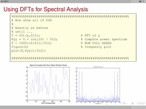
Using DFTs for Spectral Analysis%%%%%%%%%%%%%%%%%%%%%%%%%%%%%%%%%%%%%%%%%%%%%%%%%%%%%%%%%%%%%% Now show all of PSD%% Exactly as before% until ...Y = fft(y,512); % FFT of yPyy = Y.* conj(Y) / 512; % Compute power spectrumf = 1000*(0:511)/512; % NOW FULL RANGEfigure(2) % frequency plotplot(f,Pyy(1:512))
%%%%%%%%%%%%%%%%%%%%%%%%%%%%%%%%%%%%%%%%%%%%%%%%%%%%%%%%%%%%%
0 10 20 30 40 50−4
−3
−2
−1
0
1
2
3
4Signal Corrupted with Zero−Mean Random Noise
time (milliseconds)0 100 200 300 400 500 600 700 800 900 1000
0
10
20
30
40
50
60
70
80
90Frequency content of y
frequency (Hz)
A1 2011 35 / 1
♣ Example: Comparing DFT with analytical
[Q] Compare the FT and sampled DFTs of x(t) = u(t)e−t with asample interval of 0.1 s and N = 64.[A]
FT[u(t)e−t] =
∫ ∞0
e−(t+iωt)dt =1
1 + i2πf
Compute the DFT using the fft function in Matlab ...
A1 2011 36 / 1
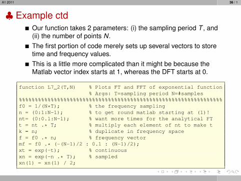
♣ Example ctdOur function takes 2 parameters: (i) the sampling period T , and(ii) the number of points N.The first portion of code merely sets up several vectors to storetime and frequency values.This is a little more complicated than it might be because theMatlab vector index starts at 1, whereas the DFT starts at 0.
function L7_2(T,N) % Plots FT and FFT of exponential function% Args: T=sampling period N=#samples
%%%%%%%%%%%%%%%%%%%%%%%%%%%%%%%%%%%%%%%%%%%%%%%%%%%%%%%%%%%%%%%%f0 = 1/(N*T); % the frequency samplingn = (0:1:N-1); % to get round matlab starting at (1)!nt= (0:0.1:N-1); % want more times for the analytical FTt = nt .* T; % multiply each element of nt to make tk = n; % duplicate in frequency spacef = f0 .* n; % frequency vectormf = f0 .* (-(N-1)/2 : 0.1 : (N-1)/2);xt = exp(-t); % continuousxn = exp(-n .* T); % sampledxn(1) = xn(1) / 2;
A1 2011 37 / 1
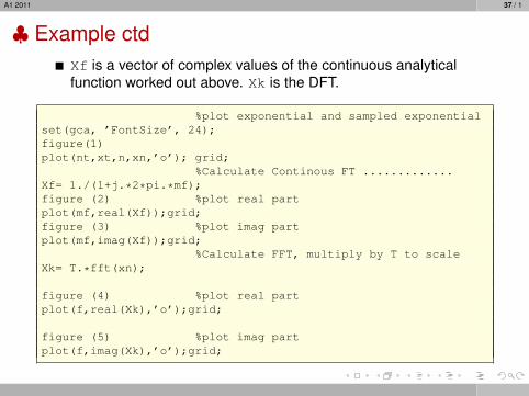
♣ Example ctdXf is a vector of complex values of the continuous analyticalfunction worked out above. Xk is the DFT.
%plot exponential and sampled exponentialset(gca, ’FontSize’, 24);figure(1)plot(nt,xt,n,xn,’o’); grid;
%Calculate Continous FT .............Xf= 1./(1+j.*2*pi.*mf);figure (2) %plot real partplot(mf,real(Xf));grid;figure (3) %plot imag partplot(mf,imag(Xf));grid;
%Calculate FFT, multiply by T to scaleXk= T.*fft(xn);
figure (4) %plot real partplot(f,real(Xk),’o’);grid;
figure (5) %plot imag partplot(f,imag(Xk),’o’);grid;
A1 2011 38 / 1
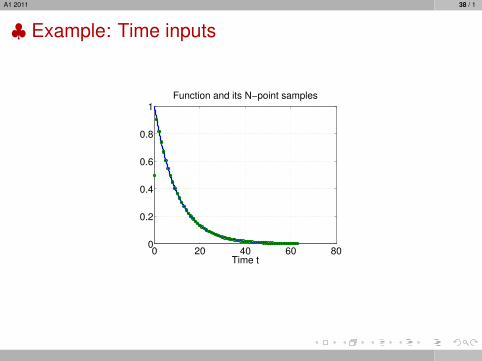
♣ Example: Time inputs
0 20 40 60 800
0.2
0.4
0.6
0.8
1Function and its N−point samples
Time t

A1 2011 39 / 1
Output — real parts compared
−5 −4 −3 −2 −1 0 1 2 3 4 50
0.1
0.2
0.3
0.4
0.5
0.6
0.7
0.8
0.9
1Real part of continous FT
Frequency (Hz)0 1 2 3 4 5 6 7 8 9 10
0
0.1
0.2
0.3
0.4
0.5
0.6
0.7
0.8
0.9
1Real part of DFT
Frequency (Hz)
Real Pt of 1/(1 + i2πf ) Real Pt of DFT
A1 2011 40 / 1
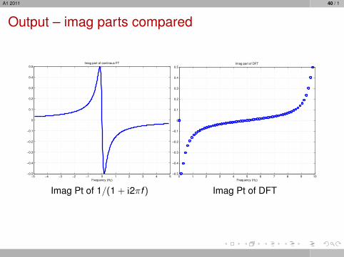
Output – imag parts compared
−5 −4 −3 −2 −1 0 1 2 3 4 5−0.5
−0.4
−0.3
−0.2
−0.1
0
0.1
0.2
0.3
0.4
0.5Imag part of continous FT
Frequency (Hz)0 1 2 3 4 5 6 7 8 9 10
−0.5
−0.4
−0.3
−0.2
−0.1
0
0.1
0.2
0.3
0.4
0.5Imag part of DFT
Frequency (Hz)
Imag Pt of 1/(1 + i2πf ) Imag Pt of DFT
A1 2011 41 / 1
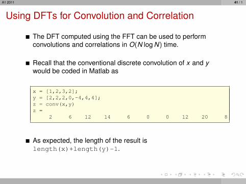
Using DFTs for Convolution and Correlation
The DFT computed using the FFT can be used to performconvolutions and correlations in O(N log N) time.
Recall that the conventional discrete convolution of x and ywould be coded in Matlab as
x = [1,2,3,2];y = [2,2,2,0,-4,4,4];z = conv(x,y)z =
2 6 12 14 6 0 0 12 20 8
As expected, the length of the result islength(x)+length(y)-1.
A1 2011 42 / 1
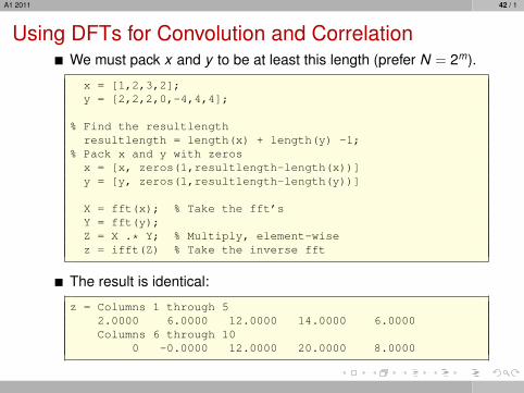
Using DFTs for Convolution and CorrelationWe must pack x and y to be at least this length (prefer N = 2m).
x = [1,2,3,2];y = [2,2,2,0,-4,4,4];
% Find the resultlengthresultlength = length(x) + length(y) -1;
% Pack x and y with zerosx = [x, zeros(1,resultlength-length(x))]y = [y, zeros(1,resultlength-length(y))]
X = fft(x); % Take the fft’sY = fft(y);Z = X .* Y; % Multiply, element-wisez = ifft(Z) % Take the inverse fft
The result is identical:
z = Columns 1 through 52.0000 6.0000 12.0000 14.0000 6.0000Columns 6 through 10
0 -0.0000 12.0000 20.0000 8.0000
A1 2011 43 / 1
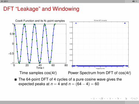
DFT “Leakage” and Windowing
0 20 40 60 80−1
−0.5
0
0.5
1Cos4t Function and its N−point samples
Time t 0 1 2 3 4 5 6 7 8 9 100
0.02
0.04
0.06
0.08
0.1
0.12
0.14
0.16PS from DFT of cos(4t)
Frequency (Hz)
Time samples cos(4t) Power Spectrum from DFT of cos(4t)
The 64-point DFT of 4 cycles of a pure cosine wave gives theexpected peaks at n = 4 and n = (64− 4) = 60
A1 2011 44 / 1
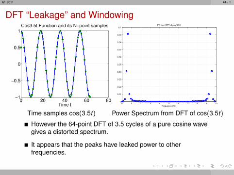
DFT “Leakage” and Windowing
0 20 40 60 80−1
−0.5
0
0.5
1Cos3.5t Function and its N−point samples
Time t 0 1 2 3 4 5 6 7 8 9 100
0.01
0.02
0.03
0.04
0.05
0.06
0.07
0.08
0.09
0.1PS from DFT of cos(3.5t)
Frequency (Hz)
Time samples cos(3.5t) Power Spectrum from DFT of cos(3.5t)
However the 64-point DFT of 3.5 cycles of a pure cosine wavegives a distorted spectrum.
It appears that the peaks have leaked power to otherfrequencies.
A1 2011 45 / 1
DFT “Leakage” and Windowing
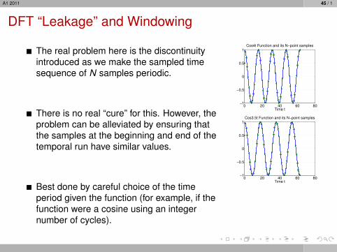
The real problem here is the discontinuityintroduced as we make the sampled timesequence of N samples periodic.
There is no real “cure” for this. However, theproblem can be alleviated by ensuring thatthe samples at the beginning and end of thetemporal run have similar values.
Best done by careful choice of the timeperiod given the function (for example, if thefunction were a cosine using an integernumber of cycles).
0 20 40 60 80−1
−0.5
0
0.5
1Cos4t Function and its N−point samples
Time t
0 20 40 60 80−1
−0.5
0
0.5
1Cos3.5t Function and its N−point samples
Time t
A1 2011 46 / 1
DFT “Leakage” and Windowing
When this is not possible ...Avoid using a top-hat window w(t).Use an apodization or tapering function which brings the samplesdown to zero at the edges of the sampled region.
This suppresses the sidelobes in W (f ) which would otherwise beproduced.
However, the central region of W (f ) becomes wider. In turn thiswidens the lines in the frequency spectrum, decreasing theresolution.
There are many such functions — examples are the Gaussian,the Hamming window, and the von Hann (or Hanning function)window.
A1 2011 47 / 1
DFT “Leakage” and Windowing
Another way of looking at the use of such functions is that theyreduce the asymmetry in the way that temporal sampling andfrequency sampling is performed.
Using a top hat w(t) and sinc function W (f ) led to the x [n]containing no error and the X [k ] containing all the error.
![LOAD-FREQUENCY CONTROL AND PERFORMANCE · A1 – Appendix 1: Load-Frequency Control and Performance [E] Chapters A. Primary Control B. Secondary Control C. Tertiary Control D. Time](https://img.pdfslide.net/doc/110x75/5e9f3f5f6fb550227a4ed9bc/load-frequency-control-and-performance-a1-a-appendix-1-load-frequency-control.jpg)