1

MULTI-OBJECTIVE OPTIMISATION OF MANY-REVOLUTION, LOW-THRUST ORBIT RAISING FOR DESTINY MISSION

Federico Zuiani *, Yasuhiro Kawakatsu † and Massimiliano Vasile ‡

This work will present a Multi-Objective approach to the design of the initial, Low-Thrust orbit raising phase for JAXA’s proposed technology demonstrator mission DESTINY. The proposed approach includes a simplified model for Low Thrust, many-revolution transfers, based on an analytical orbital averaging tech-nique, and a simplified control parameterisation. Eclipses and J2 perturbation are also accounted for. This is combined with a stochastic optimisation algorithm to solve optimisation problems in which conflicting performance figures of DESTINY’s trajectory design are concurrently optimised. It will be shown that the proposed approach provides for a good preliminary investigation of the launch window and helps identifying critical issues to be addressed in future de-sign phases.

INTRODUCTION

The Demonstration and Experiment for Space Technology and INterplanetary voYage (DESTINY)1 is a technology demonstrator mission which is currently being developed as a can-didate third mission of ISAS/JAXA’s small science satellite series. Its main objective is that of gaining flight heritage for a number of novel technologies, which include, among others, the new µ20 Ion engine, the new Epsilon launch vehicle, ultra-lightweight solar panels and an advanced thermal control. In addition, it will also provide a test-bed for new techniques for Low Thrust (LT), interplanetary mission design and operation.

The proposed mission profile for DESTINY, as shown in Figure 1, envisions:

1) Injection into an inclined elliptical orbit (with semi-major axis around 20000 km) by means of the Epsilon rocket.

2) Spiralling phase in which the µ20 engine will raise the orbit in order to encounter the Moon.

3) Lunar swing-by. 4) Injection into a Halo orbit at the Sun-Earth L2 Point. 5) Additionally, if possible, a final escape from L2 is also desirable.

* Ph.D. Candidate, School of Engineering, University of Glasgow, James Watt South Building, Glasgow G12 8QQ, United Kingdom. E-mail: f.zuiani.1@research.gla.ac.uk. Currently at ISAS/JAXA as JSPS Fellow. † Associate Professor, Institute of Space and Astronautical Science, Japan Aerospace Exploration Agency, 3-1-1 Yoshino-dai, Chuo-ku, Sagamihara-shi, Kanagawa-ken, 252-5210, Japan. E-mail: kawakatsu.yasuhiro@jaxa.jp ‡ Reader, Department of Mechanical and Aerospace Engineering, University of Strathclyde, Graham Hills Building, 50 George Street, Glasgow G1 1QE, United Kingdom. E-mail: massimiliano.vasile@strath.ac.uk

AAS 13-264

2

Figure 1. DESTINY preliminary mission profile.

The early LT orbit raising phase presents an interesting mission design challenge, since a many trade-offs are to be made between different performance figures; at the same time, techno-logical limitations from bus design impose a number of constraints on trajectory design. In par-ticular, the time to reach the Moon encounter is upper bounded at 1.5 years but shorter transfer times might also be advantageous. On the other hand, in the latter case, the required ∆V is likely to be higher; while this, given the available fuel and the high efficiency of the µ20 engine, will not prevent reaching the Halo orbit, it will possibly affect the feasibility of the optional post-Halo escape phase. It should also be noted that, during the orbit raising phase the spacecraft will spend a long period of time within the highly radiative environment of the Van Allen belts. This time should be minimised in order to reduce the total radiation dose and therefore the mass of the re-quired shielding for electronic components. Similarly, eclipse duration during the transfer, influ-ences both trajectory design, since engine operation has to be interrupted while in shadow, and spacecraft bus design because it imposes constraints on battery sizing. Finally the conditions, in terms of orbit geometry, with which the Moon is encountered, also require trade-off analysis, since they are strongly linked with the trajectory design of the following phase which will lead DESTINY spacecraft to the designated L2 Halo orbit.

The presence of many conflicting requirements will be tackled in this work by adopting a Multi-Objective (MO) design approach, in which multiple performance figures are concurrently optimised. Multi-objective design of Low-Thrust trajectories is a challenging optimisation prob-lem and the reasons for this are twofold: first, the computation of a single LT transfer is already a complex problem because it generally requires the solution of a Low-Thrust, Two Point, Bounda-ry Value Problem (LT-2PBVP), and given the complex dynamics involved and the potentially large number of control parameters this is usually computationally very expensive. Secondly, the solution of multi-objective optimisation problems is usually accomplished by means of global multi-objective stochastic algorithms which require the evaluation of a large number of candidate solutions in order to find a set of Pareto optimal ones. This fact makes the application of tradi-tional LT trajectory design techniques computationally unfeasible. Therefore, in this work a novel approach will be proposed, which combines an analytical averaging technique with a simplified parameterisation of the thrust control. The former is meant at considerably lowering the computa-tional time needed to propagate long spiralling trajectories, like the one of DESTINY, while the latter is aimed at reducing the number of parameters which define the thrusting strategy. This al-

3

lows combining the proposed analytical averaged approach with a MO optimisation algorithm2 in order to solve a complex MO problem in which hundreds of thousands candidate solutions are evaluated.

LOW THRUST, MANY-REVOLUTION TRANSFERS

In past works, other authors have already proposed approaches to the design of low thrust, many-revolution transfers. Among them, there is a good number of methods based on analytical solutions of the equations of motion, for example under the assumption of small eccentricity3,4,5; averaging techniques6,7 have also been combined direct transcription optimisation techniques. However, most of these proposals lack flexibility for treating generic many-revolution transfer problems. Adding to this, Multi-Objective LT transfer optimisation is a field which is still in its infancy.

In the proposed approach, the motion of the spacecraft is propagated by means of an orbital averaging technique, in which the net variation of the orbital elements along a single revolution is computed; then this averaged over the orbit period and the resulting quantity is integrated numer-ically over the long time periods. In particular the variation of orbital elements ∆E2π along a sin-gle revolution due to the thrust is computed by means of an analytical, first-order solution of per-turbed Keplerian motion8,9,10, which has shown to guarantee adequate accuracy at a lower compu-tational cost compared to numerical integration. The contribution of the J2 perturbation is also in-cluded. An extensive description of the analytical formulae and of their accuracy can be found in8,9,10 and will not be repeated here in detail for the sake of conciseness.

Figure 2. Thrusting pattern.

In order to keep the number of parameters low, a number of assumptions on the thrusting strategy are introduced. First of all, an on/off control is assumed, in the sense that at a given in-stant, the thrust magnitude can be either zero or the maximum value permitted by engine specifi-cations. Secondly, it is assumed that the thrust direction is purely in plane and directed along the tangential direction, which maximises the instantaneous variation of orbital energy. Thus, one has to define the timing of the thrust switching. The control parameterisation is similar to the one proposed in11, in which each revolution is divided in 4 sectors, as shown in Figure 2: a Perigee thrusting arc, an Apogee thrusting arc and two coasting arcs in between. The first, of amplitude ∆Lp, is meant ideally to alter apocenter altitude by thrusting in either way along the tangential di-

2 La 2 Lp

Apogee

Thrusting

arc

Coasting

arcs

Perigee

Thrusting

arc

Orbital

motion

4

rection. Similarly, the second alters the pericenter altitude by thrusting tangentially around the apoapsis for an arc of amplitude ∆La. The variation of the orbital elements along the thrusting arcs is computed with the analytical formulae. If a plane change were also required, an out-of-plane component described by elevation βp and βa, could also have been introduced, but this is not done here. Therefore, the amplitudes of the arcs ∆Lp and ∆La are the quantities to be set to define a con-trol profile.

Given the above mentioned control profile, the propagation of the equations of motion is per-formed by means of an averaging technique:

( ) ( ) ( )( )0

0

2

2

( ) , , ,t

p aavg

t

avg

t L L d

Tπ

π

τ τ τ τ τ= ∆ ∆+

∆=

∫

E

E E E E

E

ɺ

ɺ

(1)

where ∆E2π is the variation of the orbital elements computed by propagating the discontinuous control profile, as described in the previous section, over an arc of 2π. T2π is the orbital period as-sociated to this arc. As already mentioned, this propagation over 2π is performed analytically,

while the averaged variation avgEɺ is propagated with a Runge-Kutta integration method.

The terms pL∆ and aL∆ are defined as a piecewise linear interpolation with respect to time, from nnodes nodal values, uniformly spaced within the integration boundaries. For example, in the case of pL∆ , one can write:

( ) ( ), ,p interp pL t f t∆ = t ∆L (2)

where ∆L p is a vector containing the nnodes nodal values, t is the vector which collects the cor-responding times at which the nodal values are specified. finterp defines a piecewise linear interpo-lation.

In previous works9,10, it has been shown that this technique allows for a fast propagation of long, many-revolution, Low-Thrust transfers, while maintaining adequate accuracy. However, an obvious drawback is that, since the propagation of the motion is performed by averaging, all in-stantaneous information, like for example the actual position of the spacecraft along an orbit, is lost. However, for the purposes of the present preliminary analysis, this is a secondary concern and the averaged propagation is deemed as adequate in computing the figures of merit required by the Multi-Objective optimisation process.

Eclipse modelling

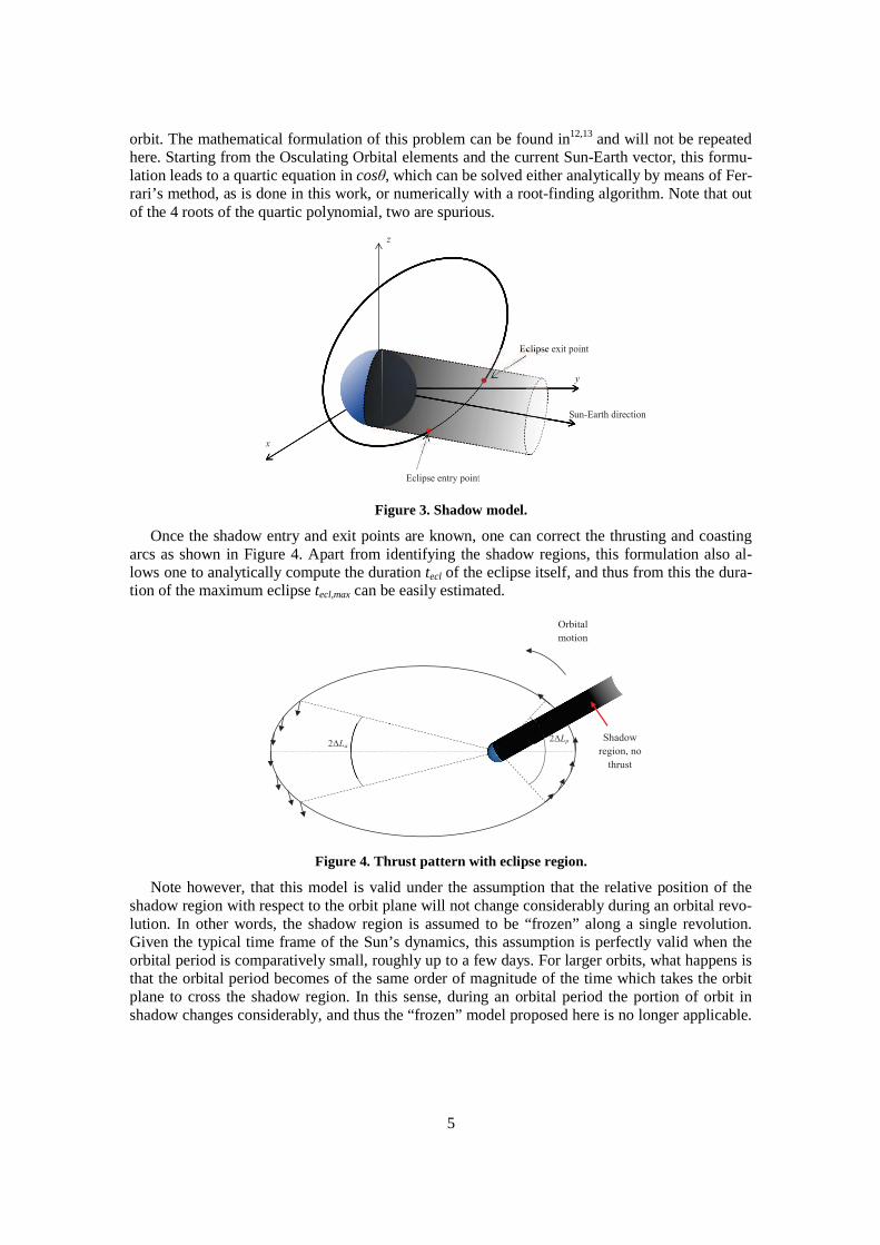
As already mentioned, one of the tasks of this study is that of minimising the maximum eclipse encountered by DESTINY during the orbit raising phase. At the same time, constraints on power generation require the interruption of engine operation while the spacecraft is in shadow. In this sense, with reference to Figure 2, along a given orbit, it is necessary to compute the eclipse entry and exit points in order to modify the thrusting strategy accordingly. In this work, a cylin-drical model for Earth’s shadow is adopted (see Figure 3), which is deemed as adequate in the case of a spacecraft in Earth orbit. In order to identify the eclipse entry and exit points one has to find the true anomalies of the geometrical intersections between the cylinder and the osculating

5

orbit. The mathematical formulation of this problem can be found in12,13 and will not be repeated here. Starting from the Osculating Orbital elements and the current Sun-Earth vector, this formu-lation leads to a quartic equation in cosθ, which can be solved either analytically by means of Fer-rari’s method, as is done in this work, or numerically with a root-finding algorithm. Note that out of the 4 roots of the quartic polynomial, two are spurious.

Figure 3. Shadow model.

Once the shadow entry and exit points are known, one can correct the thrusting and coasting arcs as shown in Figure 4. Apart from identifying the shadow regions, this formulation also al-lows one to analytically compute the duration tecl of the eclipse itself, and thus from this the dura-tion of the maximum eclipse tecl,max can be easily estimated.

Figure 4. Thrust pattern with eclipse region.

Note however, that this model is valid under the assumption that the relative position of the shadow region with respect to the orbit plane will not change considerably during an orbital revo-lution. In other words, the shadow region is assumed to be “frozen” along a single revolution. Given the typical time frame of the Sun’s dynamics, this assumption is perfectly valid when the orbital period is comparatively small, roughly up to a few days. For larger orbits, what happens is that the orbital period becomes of the same order of magnitude of the time which takes the orbit plane to cross the shadow region. In this sense, during an orbital period the portion of orbit in shadow changes considerably, and thus the “frozen” model proposed here is no longer applicable.

x

z

Eclipse entry pointt

Ec

Su

y

clipse exit po

un-Earth dire

y

oint

ection

2ΔLa 2ΔLp

Orbital

motion

2 Shadow

region, no

thrust

6

At the same time, however, it also means that there will be just a single eclipse in that revolution and not a sequence of eclipses in close succession as it happens when the orbital period is small. Therefore, it can be assumed that with proper phasing correction at some point before this single eclipse, the latter can be shortened or even avoided altogether. For this reason, it is decided here to ignore these isolated eclipses, in the computation of the maximum eclipse duration, since eclipse avoidance strategies can be easily implemented at a later, more detailed design stage.

DESTINY TRAJECTORY MODEL

The purpose of this study is that of optimising the strategy for DESTINY’s orbit raising phase in order to concurrently minimise four figures of merit: the time of flight ToF, the total Ion En-gine System operation time IES, the time spent within the radiation belt tbelt and finally the dura-tion of the maximum eclipse encountered tecl,max. The latter, in addition, is to be kept below 1 h, due to constraints on battery size. The maximum time of flight allowed for the orbit raising phase is 550 days, i.e. about 1.5 years.

As a result of the inputs from the design team of the Epsilon Launch Vehicle, the initial orbit parameters after release from the launcher are assumed to be those reported in Table 1.

Table 1. DESTINY initial orbit parameters in the J2000 Earth Fixed reference frame.

a (km) e i Ω ω M

20953 0.69 32° 21° 124° 5°

Note that, the initial orbital elements are specified with respect to the J2000 Earth Fixed refer-ence frame, i.e. a moving frame, and thus the actual value of Ω in the inertial reference frame is dependent on the launch epoch. After release from the launcher, a 30-day commissioning phase is imposed, in which the spacecraft is not allowed to perform any manoeuver.

The terminal condition to be reached at the end of the orbit phase is a radius of 300000 km at the intersection between the orbit and the current lunar orbital plane. This condition reflects the fact that at this preliminary stage it has been decided to uncouple the design of the orbit raising phase from that of the Lunar encounter and subsequent interplanetary phase. Note also that, given the relative angle between the lunar orbit plane and DESTINY’s, the intersection between the two might occur quite far from DESTINY’s apoapsis and therefore the latter might be much higher than 300000 km.

The preliminary specifications for DESTINY spacecraft are reported in Table 2.

Table 2. DESTINY spacecraft characteristics.

Initial mass (kg) Engine thrust (mN) Specific impulse (s)

400 40 3800

The powerful μ20 engine, mounted on a small spacecraft, produces a relatively high accelera-tion of 10-4 m/s2. At the same time, the high specific impulse of this ion engine ensures good pro-pellant efficiency.

7

The design parameters which are to be optimised are the departure epoch and the parameters of the thrust vector. For each candidate set for these parameters, the propagation technique pre-sented in the previous section is used to propagate the orbital until the terminal condition of 300000 km radius on the lunar orbit plane has been verified, or else when the maximum time of flight allowed, 550 days, has been reached. From this it is possible to compute the total time of flight ToF, total engine operation time IES, the time within the radiation belt tbelt and the duration of the maximum longest eclipse tecl,max. Note that, tbelt is defined simply as the time for which the spacecraft is below 20000 km altitude. The candidate parameter sets will be generated by means of a Multi-Objective optimisation algorithm.

MULTI-OBJECTIVE OPTIMISATION OF DESTINY’S ORBIT RAI SING

The design of DESTINY’s orbit raising phase can be formulated as a Multi-Objective optimi-sation problem in the form:

( )minD∈x

f x (3)

where f is the vector of the objectives:

,belt ecl maxToF IES t t = f (4)

x is the parameter vector and D is its domain. x comprises the departure epoch, decomposed as date in MJD2000 and time and the semi-aplitudes of the perigee and apogee thrusting arcs, ex-pressed as the values of ∆Lp and ∆La at 8 reference nodes, as in Eq. (2). Note that date is meant as the integer part of the number of days since epoch -0.5 MJD2000, while time is intended as the number of hours since the midnight of the day defined by date.

, , 1,...,8p i a iL Ldate time i ∆ ∆= = x ⋯ ⋯ ⋯ (5)

The reason, for which the departure epoch is here expressed as day and hour, is that prelimi-nary tests revealed that the objective functions showed wide oscillations with respect to the depar-ture epoch and that the two scales of these oscillations were of the magnitude of a day and a year. This is related to the orientation of the initial orbital plane with respect to the Ecliptic plane and the lunar plane. Since, as mentioned earlier, the initial orbital elements in Table 1 are defined as relative to the Earth, i.e. a rotating reference frame, it follows that Ω in the Equatorial inertial ref-erence frame experiences a short term evolution due to the Earth’s rotation around its axis, super-imposed to a long term variation due to the Earth’s motion in the solar system (plus other secular perturbations). Therefore, by decomposing the departure epoch into date and time, one is able to decouple these two dynamics. The boundaries for the domain D are reported in Table 3.

Table 3. Boundaries for optimisation parameters.

Variable date (d) time (h) ∆Lp,i (°) ∆La,i (°)

Lower bound 0 0 0 0

Upper bound 365 24 180 180

In summary, each transfer is described by a total of 18 optimisation parameters. Regarding the performance parameters in the vector f, as already mentioned there are four figures of merit which are to be concurrently minised, ToF, IES, tbelt and tecl,max, which would translate into a 4-objective optimisation problem. In the following sub-section, it is decided to solve a reduced 3-

8

objective problem first, without tecl,max as an objective or constraint. This is done because, general-ly speaking, a 3-objective problem is easier to visualise and analyse. It will also show how the so-lution set changes, when the fourth objective will be re-introduced and the full optimisation prob-lem solved. In both cases the Multi-Objective optimisation problem in Eq. (3) is solved with MACS2, a hybrid-memetic optimisation algorithm designed by the authors14,15.

3-Objective problem

For this 3-objective problem, MACS2 is set to run for a maximum of 3·105 function evalua-tions. Population size is set at 150 individuals, of which 30 perform social actions.

Figure 5. 3-Objective problem: a) Pareto front. Projections on the b) ToF-IES c) ToF-tbelt d) IES-

tbelt sub-spaces.

Figure 5a shows the optimal objective set. For more clarity, Figure 5b-c-d show their projec-tions on the bi-dimensional subspaces. By examining the extreme points for each objective, one can see that, for example, the minimum transfer time is around 400 days, which requires a total of 8600 hours of engine operations. On the other hand, the minimum IES solution requires around 6300 hours for a 550 days transfer. Similarly, the minimum time spent in the radiation belt is above 1400 hours. The ToF-IES projection in Figure 5b shows the typical pattern of propellant versus transfer time trade-off. This implies that any reduction in propellant consumption is paid for by an increase in transfer time and vice-versa. It is also interesting to note from Figure 5d that, in a similar way, any reduction in propellant consumption below 7300 hours invariably requires an increase in tbelt. Moreover, the minimum ToF solution is also a minimiser for tbelt. The reasons for this will be explained later in this section. Figure 6 shows the distribution of the optimal solu-tions along the launch window and shows that they are aligned along a diagonal line in the date-time space. As mentioned earlier, date and time are determining the initial Ω in the Equatorial

350 400 450 500 5506000

6500

7000

7500

8000

8500

9000

Pareto front ToF−IES, colorbar=tbelt

ToF [d]

IES

[h

]1500

1600

1700

1800

1900

2000

350 400 450 500 5501400

1600

1800

2000

2200

Pareto front ToF−tbelt

, colorbar=IES

ToF [d]

t bel

t [h

]

6500

7000

7500

8000

8500

6000 7000 8000 90001400

1600

1800

2000

2200

Pareto front IES−tbelt

, colorbar=ToF

IES [h]

t bel

t [h

]

400

450

500

300400

500600

6000

8000

100001400

1600

1800

2000

ToF [d]

Pareto front ToF−IES−tbelt

, colorbar=tbelt

IES [h]

t bel

t [h

]

1500

1600

1700

1800

1900

2000

c)

b)

d)

a)

1

3

2

9

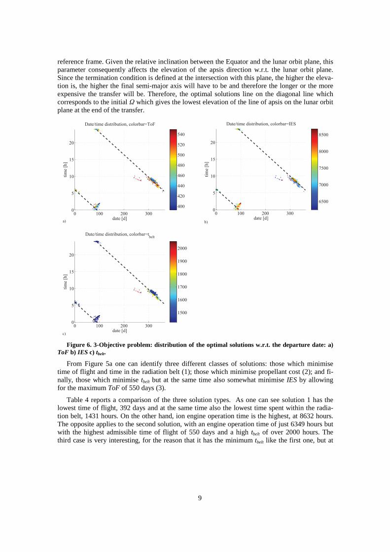
reference frame. Given the relative inclination between the Equator and the lunar orbit plane, this parameter consequently affects the elevation of the apsis direction w.r.t. the lunar orbit plane. Since the termination condition is defined at the intersection with this plane, the higher the eleva-tion is, the higher the final semi-major axis will have to be and therefore the longer or the more expensive the transfer will be. Therefore, the optimal solutions line on the diagonal line which corresponds to the initial Ω which gives the lowest elevation of the line of apsis on the lunar orbit plane at the end of the transfer.

Figure 6. 3-Objective problem: distribution of the optimal solutions w.r.t. the departure date: a)

ToF b) IES c) tbelt.

From Figure 5a one can identify three different classes of solutions: those which minimise time of flight and time in the radiation belt (1); those which minimise propellant cost (2); and fi-nally, those which minimise tbelt but at the same time also somewhat minimise IES by allowing for the maximum ToF of 550 days (3).

Table 4 reports a comparison of the three solution types. As one can see solution 1 has the lowest time of flight, 392 days and at the same time also the lowest time spent within the radia-tion belt, 1431 hours. On the other hand, ion engine operation time is the highest, at 8632 hours. The opposite applies to the second solution, with an engine operation time of just 6349 hours but with the highest admissible time of flight of 550 days and a high tbelt of over 2000 hours. The third case is very interesting, for the reason that it has the minimum tbelt like the first one, but at

0 100 200 3000

5

10

15

20

Date/time distribution, colorbar=ToF

date [d]

tim

e [h

]

400

420

440

460

480

500

520

540

0 100 200 3000

5

10

15

20

Date/time distribution, colorbar=IES

date [d]

tim

e [h

]6500

7000

7500

8000

8500

0 100 200 3000

5

10

15

20

Date/time distribution, colorbar=tbelt

date [d]

tim

e [h

]

1500

1600

1700

1800

1900

2000

a)

c)

b)

10

the same time its fuel consumption is not as high as the first case, since the time of flight has been allowed to increase up to almost 550 days.

Table 4. Summary of sample solutions

Type date (d) time (h) ToF (d) IES (h) tbelt (h)

1 min(ToF) 295 9.2 392 8632 1431

2 min(IES) 266 8.7 550 6249 2032

3 min(tbelt),max(ToF) 329 8.3 550 6865 1457

In order to better understand the differences between the three cases, Figure 7, Figure 9 and Figure 11 show the thrusting arc length and the time history of the perigee/apogee radii for each of them. From Figure 7a one can see that the semi-amplitude of the thrusting arc for the minimum ToF case is always 180 degrees (except for the initial commissioning phase), which translates in-to a continuous thrust profile. And as Figure 7b shows, perigee and apogee are concurrently raised, with a monotonic decrease of the eccentricity, which reaches 0.2 at the end of the transfer. Note also that the Apogee is around 300000 km when the terminal condition is reached, which confirms what said earlier that the optimal solutions reach the terminal condition with the line of apses lying on the lunar orbital plane.

Figure 7. Minimum ToF solution: a) thrusting arc length; b) perigee/apogee radii.

From Figure 8, which plots the trajectory in the J2000 reference frame, one can also clearly appreciate that the typical shape of a continuous tangential thrust trajectory as the orbit shape gradually becomes less eccentric.

0 100 200 300 4000

20

40

60

80

100

120

140

160

180Thrusting arc length

t [d]

∆L

p,∆

La [

deg

]

∆Lp

∆La

0 100 200 300 4000

0.5

1

1.5

2

2.5

3

3.5x 10

5 Perigee/Apogee radius

t [d]

r p,r

a [km

]

rp

ra

a) b)

11

Figure 8. Minimum ToF solution: trajectory.

From Figure 9a, one can see that for the minimum IES solution, the thrusting arcs are located always around perigee with a semi-amplitude around 150-160 degrees. Consequently, the rate of increase of the orbit size is much lower (see Figure 9b) and at the same time the effort is focused on raising the apogee while the perigee experiences only a comparatively small increase up to around 30000 km, leading to the high tbelt mentioned before.

Figure 9. Minimum IES solution: a) thrusting arc length; b) perigee/apogee radii.

0 200 400 6000

20

40

60

80

100

120

140

160

180Thrusting arc length

t [d]

∆L

p,∆

La [

deg

]

∆Lp

∆La

0 200 400 6000

0.5

1

1.5

2

2.5

3

3.5x 10

5 Perigee/Apogee radius

t [d]

r p,r

a [k

m]

rp

ra

a) b)

12

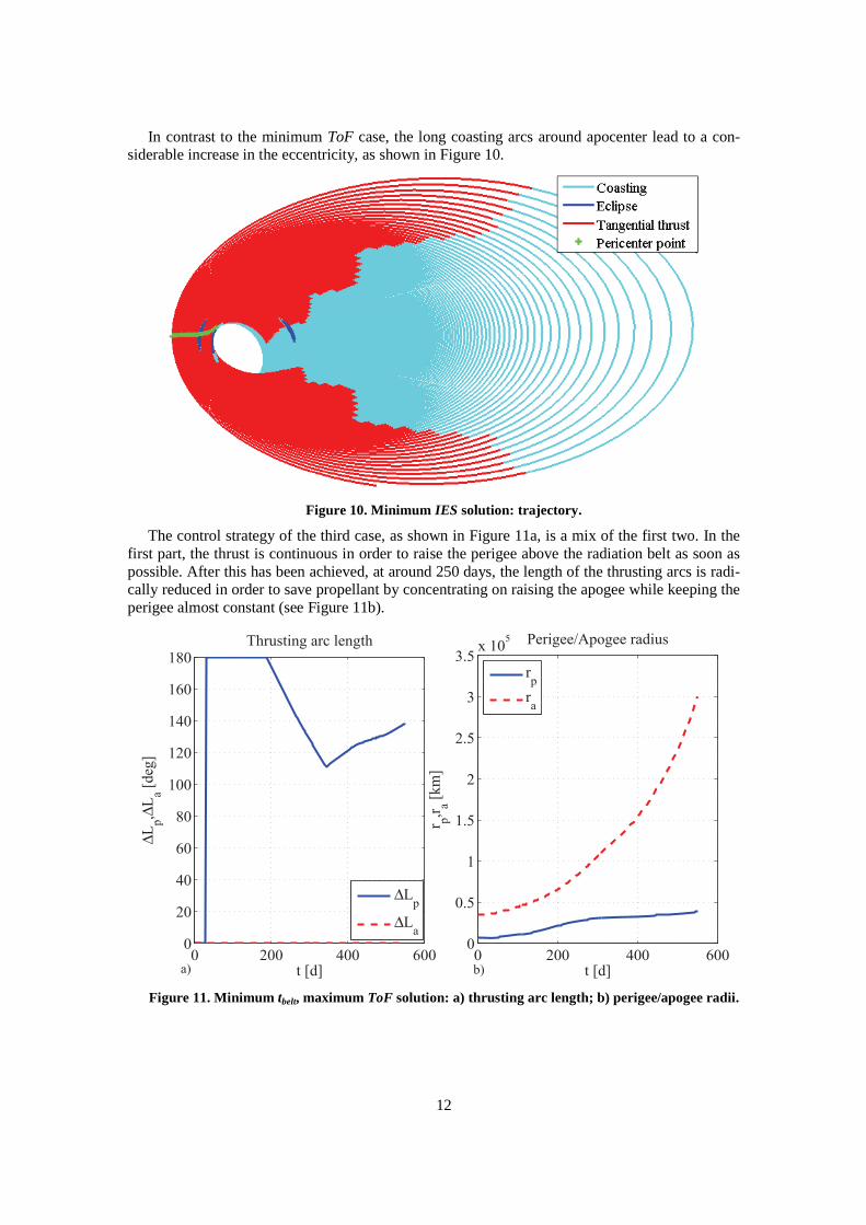
In contrast to the minimum ToF case, the long coasting arcs around apocenter lead to a con-siderable increase in the eccentricity, as shown in Figure 10.

Figure 10. Minimum IES solution: trajectory.

The control strategy of the third case, as shown in Figure 11a, is a mix of the first two. In the first part, the thrust is continuous in order to raise the perigee above the radiation belt as soon as possible. After this has been achieved, at around 250 days, the length of the thrusting arcs is radi-cally reduced in order to save propellant by concentrating on raising the apogee while keeping the perigee almost constant (see Figure 11b).

Figure 11. Minimum tbelt, maximum ToF solution: a) thrusting arc length; b) perigee/apogee radii.

0 200 400 6000

20

40

60

80

100

120

140

160

180Thrusting arc length

t [d]

∆L

p,∆

La [

deg

]

∆Lp

∆La

0 200 400 6000

0.5

1

1.5

2

2.5

3

3.5x 10

5 Perigee/Apogee radius

t [d]

r p,r

a [km

]

rp

ra

a) b)

13

Figure 12 shows a view of the complete trajectory and clearly reveals the uninterrupted thrust-ing strategy in the initial part of the trajectory, followed by a phase with long coasting arcs around apocenter which lead to a gradual increase of the eccentricity, which is however lower than in the previous case.

Figure 12. Minimum tbelt, maximum ToF solution:trajectory.

14

4-Objective problem

For the 4-objective case, MACS2 is run for a total of 6·105 function evaluations.

Figure 13. 4-Objective problem: Projections of the 4-dimensional Pareto set on the a) ToF-IES b)

tbelt-tecl,max c) ToF-tbelt d) IES-tbelt e) ToF-tecl,max f) IES-tecl,max sub-spaces. Black asterisks denote solu-tions with tecl,max≤1 h.

Figure 13 shows the set of the Pareto-optimal solutions, projected onto each of the bi-dimensional sub-spaces. Black asterisks denote the solutions which have the longest eclipse be-low 1 hour. In this respect, it is immediately apparent that there is no feasible solution with IES below 8000 hours (see Figure 13a). Similarly, from Figure 13b one can see that all these solutions have tbelt which is 1600 hours at most. This suggests that, in this case, solutions with a fast initial orbit raising phase are optimal for avoiding eclipses.

350 400 450 500 5506000

7000

8000

9000

Pareto front ToF−IES, colorbar=tbelt

ToF [d]

IES

[h]

1500

1600

1700

1800

1900

2000

350 400 450 500 5501400

1600

1800

2000

2200

Pareto front ToF−tbelt

, colorbar=IES

ToF [d]

t bel

t [h]

6500

7000

7500

8000

8500

6000 7000 8000 90001400

1600

1800

2000

2200

Pareto front IES−tbelt

, colorbar=ToF

IES [h]

t bel

t [h]

400

450

500

350 400 450 500 5500

2

4

6

Pareto front ToF−tbelt

, colorbar=IES

ToF [d]

t eclm

ax [

h]

6500

7000

7500

8000

8500

6000 7000 8000 90000

2

4

6

Pareto front IES−tbelt

, colorbar=ToF

IES [h]

t eclm

ax [

h]

400

450

500

1400 1600 1800 2000 22000

2

4

6

Pareto front IES−tbelt

, colorbar=ToF

tbelt

[h]

t eclm

ax [

h]

400

450

500

a)

c)

e)

b)

d)

f)

15

Figure 14. 4-Objective problem: distribution of the optimal solutions w.r.t. the departure date: a)

ToF b) IES c) tbelt d) tecl,max. Black asterisks denote solutions with tecl,max≤1 h.

Figure 14 shows the distribution of the optimal solutions with respect to departure date and departure time. Generally speaking, their distribution is similar to that of the 3-objective case shown in Figure 6, as they are roughly aligned along a diagonal line. Solutions with a feasible eclipse, however, are restricted to a very small region around 24/0 h and 365/0 days, at the cor-ners in Figure 14 (Note that, due to the annual periodicity of the Earth system, the regions at the four corners of the date/time plot, are by all practical means contiguous). This clearly shows that the introduction of the upper boundary on the maximum eclipse time is considerably limiting the launch opportunities and their performance, at least under the control model adopted. At the same time, however, it is important to consider that the solution of the Multi-Objective optimisation problem as formulated in (3) will return only the globally optimal solutions. This means that fea-sible, although inferior, solutions might still exist for other departure dates but, since they are dominated by other solutions, they are discarded during the optimisation process. On the other hand, at the preliminary design stage, it is desirable to investigate the existence of feasible solu-tions in less optimal regions of the launch window as well. This could also provide a good data-base of back-up solutions, should the optimal period for departure, as shown in Figure 14, be-come unfeasible due to other factors. A simple way to perform this kind of analysis would be to partition the parameter space (see Table 3) in a number of subsets along the date coordinate, and run separate Multi-Objective optimisation instances in each of them. However, this would require

0 100 200 3000

5

10

15

20

Date/time distribution, colorbar=ToF

date [d]

tim

e [h

]

400

420

440

460

480

500

520

540

0 100 200 3000

5

10

15

20

Date/time distribution, colorbar=IES

date [d]

tim

e [h

]

6500

7000

7500

8000

8500

0 100 200 3000

5

10

15

20

Date/time distribution, colorbar=tbelt

date [d]

tim

e [h

]

1500

1600

1700

1800

1900

2000

0 100 200 3000

5

10

15

20

Date/time distribution, colorbar=teclmax

date [d]

tim

e [h

]

1

1.5

2

2.5

3

3.5

4

4.5

5

a)

c) d)

b)

16

as many optimisation instances as the partitions of the domain D and at the same time, the fact that they would run separately would prevent an exchange of information between each of them. Therefore, the following alternative has been adopted, which requires only a single MO instance, and which consists in modifying the 4-Objective problem in (3) by adding two dummy perfor-mance parameters to f, as:

, 1365 365belt ecl max

date dateToF IES t t = −

f (6)

This modification makes such that a solution, even if it is inferior to another with regard to ToF, IES, tbelt or tecl,max, is still not discarded by the optimisation algorithm as long as its departure date is different from the other. Or, in other words, the optimiser will automatically search for and store the optimal solutions, in terms of ToF, IES, tbelt or tecl,max, for each departure date. This mod-ified 4-objective problem, formally a 6-objective one, is again solved with MACS2, with 106 function evaluations.

Figure 15. Modified 4-Objective problem: distribution of the optimal solutions with tecl,max≤1 h

w.r.t. the departure date: a) ToF b) IES c) tbelt d) tecl,max.

Figure 15 shows the distribution of optimal solutions with maximum eclipse duration shorter than 1 hour and reveals the existence of two new clusters of solutions in addition to those already identified in the previous, 4-objective case. One lies in the summer period close to midnight time while the other is in autumn in the 15-20 h range. Although they differ slightly in terms of per-formance parameters, a number of considerations apply to both groups. First, they both have a higher time of flight than the winter/midnight class, ranging from 480 to 550 days. At the same time, their propellant cost is also quite high, as is tbelt, which is between 2000 and 2600 hours. As

0 100 200 3000

5

10

15

20

Date/time distribution, colorbar=ToF

date [d]

tim

e [h

]

400

420

440

460

480

500

520

540

0 100 200 3000

5

10

15

20

Date/time distribution, colorbar=IES

date [d]

tim

e [h

]

8000

8100

8200

8300

8400

8500

8600

8700

0 100 200 3000

5

10

15

20

Date/time distribution, colorbar=tbelt

date [d]

tim

e [h

]

1600

1800

2000

2200

2400

2600

0 100 200 3000

5

10

15

20

Date/time distribution, colorbar=teclmax

date [d]

tim

e [h

]

0.8

0.85

0.9

0.95

a)

c) d)

b)

17

an example, Table 5 reports the relevant parameters for a typical solution in this group, which can be compared to those in Table 4. Figure 16 plots its thrusting arc length and time history of peri-gee and apogee radii.

Table 5. Sample solution in Summer with feasible eclipse.

date (d) time (h) ToF (d) IES (h) tbelt (h) tecl,max (h)

198 23.3 498 8581 2140 0.92

Figure 16. Summer solution with feasible eclipse: a) thrusting arc length; b) perigee/apogee radii.

As Figure 16a shows, at the beginning, the thrusting arcs are located around perigee with a semi-amplitude of 120 degrees, which then progressively increases to 180 degrees (i.e. continu-ous thrust) at 250 days. This might seem quite odd at first since it has the obvious drawback of increasing both the total transfer time and the exposure to the environment of the radiation belts, as testified by Table 5. Moreover, the relative geometry between the spacecraft’s orbit and the lu-nar one is far from optimal because, as can be seen in Figure 16b, the final apogee is well above 300000km, which means that the intersection with the lunar orbit plane is far from the line of apses. On the other hand, it is important to keep in mind that the driving factor for which this candidate solution has been selected is its low maximum eclipse duration. In this sense, the con-trol profile is meant at altering the geometry relative geometry between DESTINY’s orbit and the shadow region in order to minimise eclipse duration. While a more detailed discussion of the spe-cific issues of eclipses during DESTINY’s orbit raising and related avoidance techniques will be the topic of a future work, it is still important to introduce here a number of observations. First, one has to consider that, due to the relatively high inclination of DESTINY’s orbit with respect to the Ecliptic, and due to the periodicity of the apparent motion of the Sun around the Earth, the shadow region will intersect the orbit plane at more or less regular intervals. Therefore, eclipses are typically encountered in a number of separate phases. In other words, there will be parts of the

0 200 400 6000

20

40

60

80

100

120

140

160

180Thrusting arc length

t [d]

∆L

p,∆

La [

deg

]

∆Lp

∆La

0 100 200 300 400 5000

0.5

1

1.5

2

2.5

3

3.5

4x 10

5 Perigee/Apogee radius

t [d]

r p,r

a [km

]

rp

ra

a) b)

18

transfer in which there is one eclipse per orbit, separated by phases in which there are no eclipses at all.

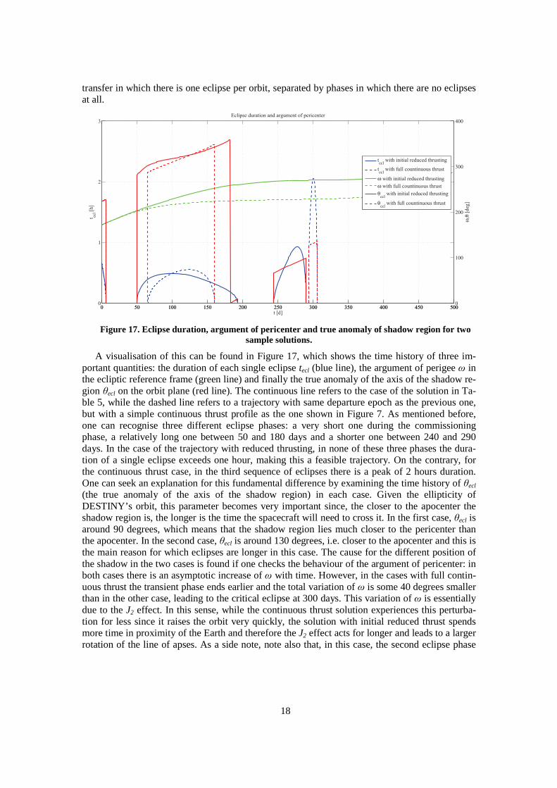
Figure 17. Eclipse duration, argument of pericenter and true anomaly of shadow region for two

sample solutions.

A visualisation of this can be found in Figure 17, which shows the time history of three im-portant quantities: the duration of each single eclipse tecl (blue line), the argument of perigee ω in the ecliptic reference frame (green line) and finally the true anomaly of the axis of the shadow re-gion θecl on the orbit plane (red line). The continuous line refers to the case of the solution in Ta-ble 5, while the dashed line refers to a trajectory with same departure epoch as the previous one, but with a simple continuous thrust profile as the one shown in Figure 7. As mentioned before, one can recognise three different eclipse phases: a very short one during the commissioning phase, a relatively long one between 50 and 180 days and a shorter one between 240 and 290 days. In the case of the trajectory with reduced thrusting, in none of these three phases the dura-tion of a single eclipse exceeds one hour, making this a feasible trajectory. On the contrary, for the continuous thrust case, in the third sequence of eclipses there is a peak of 2 hours duration. One can seek an explanation for this fundamental difference by examining the time history of θecl (the true anomaly of the axis of the shadow region) in each case. Given the ellipticity of DESTINY’s orbit, this parameter becomes very important since, the closer to the apocenter the shadow region is, the longer is the time the spacecraft will need to cross it. In the first case, θecl is around 90 degrees, which means that the shadow region lies much closer to the pericenter than the apocenter. In the second case, θecl is around 130 degrees, i.e. closer to the apocenter and this is the main reason for which eclipses are longer in this case. The cause for the different position of the shadow in the two cases is found if one checks the behaviour of the argument of pericenter: in both cases there is an asymptotic increase of ω with time. However, in the cases with full contin-uous thrust the transient phase ends earlier and the total variation of ω is some 40 degrees smaller than in the other case, leading to the critical eclipse at 300 days. This variation of ω is essentially due to the J2 effect. In this sense, while the continuous thrust solution experiences this perturba-tion for less since it raises the orbit very quickly, the solution with initial reduced thrust spends more time in proximity of the Earth and therefore the J2 effect acts for longer and leads to a larger rotation of the line of apses. As a side note, note also that, in this case, the second eclipse phase

0 50 100 150 200 250 300 350 400 450 5000

1

2

3Eclipse duration and argument of pericenter

t [d]

t ecl [

h]

0 50 100 150 200 250 300 350 400 450 5000

100

200

300

400

ω,θ

[deg

]

tecl

with initial reduced thrusting

tecl

with full countinuous thrust

ω with initial reduced thrusting

ω with full countinuous thrust

θecl

with initial reduced thrusting

θecl

with full countinuous thrust

19

lasts longer and the third one is encountered at an earlier date than in the continuous thrust case. Without entering into too much detail, this is due to the fact the rotation of the line of nodes of the orbit is different in the two cases, again due to the different action of the J2 perturbation.

In summary, it can be said that this solution is exploiting the J2 perturbation to passively rotate the line of apses and obtain a favourable relative geometry with the shadow region in order to avoid long eclipses. In order to obtain this, of course, it sacrifices time of flight and transit time in the radiation belt and consequently it is not a globally optimal transfer but nevertheless it consti-tutes a feasible alternative if a departure date in seasons other than winter becomes imperative.

CONCLUSIONS

This paper presented the preliminary design of the initial, Low-Thrust orbit raising phase for DESTINY mission. Multiple design drivers and constraints were taken into account by formulat-ing the design problem as a Multi-Objective optimisation problem. The high computational cost and number of parameters related to Low-Thrust trajectory design was overcome by adopting an averaged analytical propagation technique and by using a simplified control parameterisation. The MO problem was solved by means of a stochastic global optimisation algorithm. The results obtained provided a good picture of the different transfer options and their inherent trade-offs. At the same time, detailed analysis of the results allowed for a better understanding of the dynamics of the orbit raising problem. In particular, the constraint on maximum eclipse duration was shown to be a very critical requirement, which restricts the optimal departure opportunities to the win-ter/midnight range. However, if sub-optimal solutions are also considered, transfer opportunities are available for 75% of the year, albeit with a high transit time within the radiation belts. Analy-sis of some of these solutions also suggested possible control strategies aimed specifically at avoiding long eclipses, and these will be the topic of a future work.

REFERENCES 1 Kawakatsu, Y. and Iwata, T.: DESTINY Mission Overview - A Small Satellite Mission for Deep Space Exploration Technology Demonstration, The 13th International Space Conference of Pacific‐basin Societies, 2012. 2 Vasile, M. and Zuiani, F.: Multi-agent collaborative search: an agent-based memetic multi-objective optimization al-gorithm applied to space trajectory design, Proceedings of the Institution of Mechanical Engineers, Part G: Journal of Aerospace Engineering, 2011. 3 Kechichian, J.A.: Low-Thrust Eccentricity-Constrained Orbit Raising, Journal of Spacecraft and Rockets, Vol. 35, 327-335, 1998.

4 Kechichian, J.A.: Orbit Raising with Low-Thrust Tangential Acceleration in Presence of Earth Shadow, Journal of Spacecraft and Rockets, Vol. 35, 516-525, 1998. 5 Casalino, L. and Colasurdo, G.: Improved Edelbaum's Approach to Optimize Low Earth/Geostationary Orbits Low-thrust Transfers, Journal of Guidance, Control, and Dynamics, Vol. 30, Nr. 5, 1504-1510, 2007. 6 Kluever, C.A. and Oleson, S.R.: Direct approach for computing near-optimal low-thrust earth-orbit transfers, Journal of Spacecraft and Rockets, Vol. 35, No. 4, 509-515, AIAA, 1998. 7 Gao, Y. and Li, X.: Optimization of low-thrust many-revolution transfers and Lyapunov-based guidance, Acta Astro-nautica, Vol. 66, No. 1, 117-129, Elsevier, 2010. 8 Zuiani, F., Vasile, M., Palmas, A. and Avanzini, G.: Direct transcription of low-thrust trajectories with finite trajecto-ry elements, Acta Astronautica, Vol.72, 108-120, Elsevier 2012.

20

9 Zuiani, F. and Vasile, M.: Extension of Finite Perturbative Elements for Multi-Revolution, Low-Thrust propulsion transfer optimisation, 63th International Astronautical Congress (IAC2012), IAC-12-C.1.4.6, Naples, October 1st-5th, 2012. 10 Zuiani, F. and Vasile, M.: Extended Analytical Formulas for Low-Thrust Trajectory Design, Celestial Mechanics and Dynamical Astronomy, 2013 (Submitted). 11 Zuiani, F. and Vasile, M.: Preliminary design of Debris removal missions by means of simplified models for Low-Thrust, many-revolution transfers, International Journal of Aerospace Engineering, Hindawi 2012. 12 Escobal, P.: Methods of Orbit Determination, New York, John Wiley and Sons, 1965. 13 Vallado, D.A.: Fundamentals of Astrodynamics and Applications, 3rd edition, Space Technology Library, Springer, 2007. 14 Zuiani, F. and Vasile, M.: Multi-Agent Collaborative Search with Tchebycheff decomposition and Monotonic Basin Hopping steps, BIOMA2012, Bohinij, Slovenia, 2012. 15 Zuiani, F. and Vasile, M.: Multi-Agent Collaborative Search based on Tchebycheff decomposition, Computational Optimisation and Applications, Accepted, 2013.