Multi-objective design optimisation of rolling …web.eecs.umich.edu/~shangupt/publications/sgupta-mamt07.pdf · Multi-objective design optimisation of rolling bearings ... Only the

Mechanism

Mechanism and Machine Theory 42 (2007) 1418–1443

www.elsevier.com/locate/mechmt

andMachine Theory

Multi-objective design optimisation of rolling bearingsusing genetic algorithms

Shantanu Gupta a, Rajiv Tiwari b,*, Shivashankar B. Nair a

a Department of Computer Science and Engineering, Indian Institute of Technology Guwahati, Guwahati 781039, Assam, Indiab Department of Mechanical Engineering, Indian Institute of Technology Guwahati, Guwahati 781039, Assam, India

Received 8 March 2006; received in revised form 6 September 2006; accepted 2 October 2006Available online 28 December 2006

Abstract

The design of rolling bearings has to satisfy various constraints, e.g. the geometrical, kinematics and the strength, whiledelivering excellent performance, long life and high reliability. This invokes the need of an optimal design methodology toachieve these objectives collectively, i.e. the multi-objective optimisation. In this paper, three primary objectives for a roll-ing bearing, namely, the dynamic capacity (Cd), the static capacity (Cs) and the elastohydrodynamic minimum film thick-ness (Hmin) have been optimized separately, pair-wise and simultaneously using an advanced multi-objective optimisationalgorithm: NSGA II (non-dominated sorting based genetic algorithm). These multiple objectives are performance mea-sures of a rolling bearing, compete among themselves giving us a trade-off region where they become ‘‘simultaneously opti-mal’’, i.e. Pareto optimal. A sensitivity analysis of various design parameters has been performed, to see changes in bearingperformance parameters, and results show that, except the inner groove curvature radius, no other design parameters haveadverse affect on performance parameters.� 2006 Elsevier Ltd. All rights reserved.

Keywords: Rolling bearings; Multi-objective evolutionary optimisation; NSGA II; Mechanical design; Sensitivity analysis

1. Introduction

Rolling bearings are widely used as an important component in the most of the mechanical and aerospaceengineering applications. Be it development of the house-hold appliance, automotive, space, aeronautical,micro- or nano-machine applications, all of them have given a boost to the advancement in the design tech-nology of rolling bearings. This motivated design engineers to come up with a design technology that giveslong lasting, more efficient and highly reliable bearing designs. These objectives are hard to satisfy, thus mak-ing it a numerically challenging problem. Furthermore, there is a need to optimize them collectively. Thenumerical toughness and a need to optimize them collectively warrant an application of the evolutionarymulti-objective optimisation. Objective functions for optimisation are the dynamic capacity (Cd), the static

0094-114X/$ - see front matter � 2006 Elsevier Ltd. All rights reserved.

doi:10.1016/j.mechmachtheory.2006.10.002

* Corresponding author. Tel.: +91 361 258 2667; fax: +91 361 269 0762.E-mail addresses: [email protected] (S. Gupta), [email protected] (R. Tiwari), [email protected] (S.B. Nair).

mailto:[email protected]



S. Gupta et al. / Mechanism and Machine Theory 42 (2007) 1418–1443 1419

capacity (Cs) and the elastohydrodynamic minimum film thickness (Hmin). Due to the aforementioned tough-ness of the problem, there have been very few attempts at optimizing these objectives, simultaneously.

Several research works have been reported on optimisation of various machine elements, however, very fewliteratures are available on the optimisation of rolling bearings. Asimow [1] used the Newton–Raphsonmethod for the optimum design of the length and the diameter of a journal bearing, which was supportinga given load at a given speed. The objective function was to minimize a weighted sum of the frictional lossand the shaft twist. Seireg and Ezzat [2] utilized a gradient-based search to optimise the bearing length, theradial clearance and the average viscosity of the lubricant. The objective function was chosen to minimizea weighted sum of the quantity of lubricant fed to the bearing and its temperature rise. Maday [3] and Wylieand Maday [4] used bounded variable methods of the calculus of variable, to determine the optimum config-uration for hydrodynamic bearings. The design criterion was chosen that to maximize the load carrying capa-city of the bearing. Seireg [5] reviewed some illustrative examples of the use of optimisation techniques, in thedesign of mechanical elements and systems. These include gears, journal bearings, rotating discs, pressure ves-sels, shafts under bending and torsion, beams subjected to the longitudinal impact and problems of the elasticcontact and load distributions. Hirani et al. [6] proposed a design methodology for an engine journal bearing.The procedure of selection of the diametral clearance and the bearing length was described by limiting theminimum film thickness, the maximum pressure and the maximum temperature. All the aforementioned liter-atures were concerned mainly with the journal bearing design. However, internal geometries of journal bear-ings are far simple as compared to rolling bearings.

Changsen [7] described a design method by using a gradient-based numerical optimisation technique forrolling bearings. He proposed, five objective functions for design of rolling bearings: the maximum fatigue life,the maximum wear life, the maximum static load rating, the minimum frictional moment and the minimumspin to roll ratio. The concept of optimisation of the multi-objective of rolling bearings was also proposed.Only the basic concepts and solution techniques of an optimisation problem were introduced without anyillustrations. Objective functions proposed for optimisation of rolling bearings are nonlinear in nature, more-over, associated with the geometric and kinematics constraints. Choi and Yoon [8] used GAs in optimizing theautomotive wheel-bearing unit, by considering the maximization of life of the unit as the objective function.Periaux [9] discussed in detail the application of GAs to the aeronautics and turbo machineries. Chakraborthyet al. [10] described a design optimisation problem of rolling element bearings with five design parameters, byusing GAs based on requirements of the longest fatigue life. They presented bearing internal geometricalparameters resulted from the optimised design of different bearing boundary dimensions. Main limitationsof the method were that the use of the single objective function and some of constraints were unrealistic.Assembling angles were assumed and values of other constraint constants were chosen (arbitrary) fixed tosolve the optimisation problem. Recently, Rao and Tiwari [11] developed a rolling bearing design methodol-ogy with the improved and realistic constraints for the single objective optimisation with the help of GAs.

A work on the multi-objective optimisation for the design of rolling bearings [12] does a weighted combi-nation of these individual objective functions namely – the dynamic capacity, the static capacity and the min-imum film thickness. The multi-objective problem is converted into a scalar optimisation problem. This workmade use of the deterministic as well as stochastic algorithms, for solving the constraint scalar optimisationproblem. As the deterministic approach the interior penalty function method was used, while the simulatedannealing and genetic algorithms were used as stochastic approaches. This way of combining the multiple‘competing’ objectives and optimisation of the obtained scalar objective has some prominent disadvantages– (1) a single run of the algorithm will give only one trade-off point, (2) solution points on a non-convextrade-off front cannot be obtained, and (3) no criteria for choosing weights for each of the objective functionexists. The work proposed in this paper handles each of these problems.

Any weight based combination approach has drawbacks like unknown selection of weights for differentobjectives, one point obtained in one run, and incapability to explore non-convex regions of the trade-offfront, i.e. Pareto front. Thus there is need to use a better multi-objective (evolutionary) algorithm (MOEA)for solving this problem. Coello gave a survey of the MOEA in [13]. Another survey was given in the doctoralthesis of Zitzler [14]. Because of NSGA-II’s (Elitist non-dominated sorting based genetic algorithm II) [15] lowcomputational requirements, elitist approach, and parameter-less sharing approach; it was chosen as the algo-rithm for determination of trade-off between competing performances, i.e. to generate the Pareto front [16,17].

1420 S. Gupta et al. / Mechanism and Machine Theory 42 (2007) 1418–1443

The present paper is organized as follows; Section 2 briefs the basic geometry of rolling bearings. The math-ematical model of the problem as a set of objective functions, design parameters and constraints are describedin Section 3. Section 4 introduces the concept of the multi-objective optimisation and it discusses whether adeterministic or a stochastic approach is more appropriate for this problem. Section 5 details the applicationmethodology, optimised results and the sensitivity analysis. Section 6 concludes the present work, and is fol-lowed by important references. Results obtained are satisfactory, and give a good insight into the trade-offsamong the performance measures of rolling bearings. Apart from the numerical significance of the obtainedoptimal solution, these results can help us in better understanding the parameters behind the effective design-ing of rolling bearings.

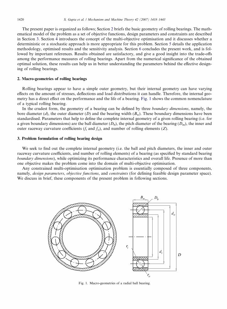
2. Macro-geometries of rolling bearings

Rolling bearings appear to have a simple outer geometry, but their internal geometry can have varyingeffects on the amount of stresses, deflections and load distributions it can handle. Therefore, the internal geo-metry has a direct effect on the performance and the life of a bearing. Fig. 1 shows the common nomenclatureof a typical rolling bearing.

In the crudest form, the geometry of a bearing can be defined by three boundary dimensions, namely, thebore diameter (d), the outer diameter (D) and the bearing width (Bw). These boundary dimensions have beenstandardised. Parameters that help to define the complete internal geometry of a given rolling bearing (i.e. fora given boundary dimensions) are the ball diameter (Db), the pitch diameter of the bearing (Dm), the inner andouter raceway curvature coefficients (fi and fo), and number of rolling elements (Z).

3. Problem formulation of rolling bearing design

We seek to find out the complete internal geometry (i.e. the ball and pitch diameters, the inner and outerraceway curvature coefficients, and number of rolling elements) of a bearing (as specified by standard bearingboundary dimensions), while optimizing its performance characteristics and overall life. Presence of more thanone objective makes the problem come into the domain of multi-objective optimisation.

Any constrained multi-optimisation optimisation problem is essentially composed of three components,namely, design parameters, objective functions, and constraints (for defining feasible design parameter space).We discuss in brief, these components of the present problem in following sections.

O .319

D

od

id

Bw

ir

or

bD

Fig. 1. Macro-geometries of a radial ball bearing.


3.1. Design parameters

The design parameter vector can be written as:

X ¼ ½Dm;Db; Z; fi; fo;KDmin;KDmax; e; e; f�; ð1Þ
where,
fi ¼ ri=Db; f o ¼ ro=Db: ð2Þ
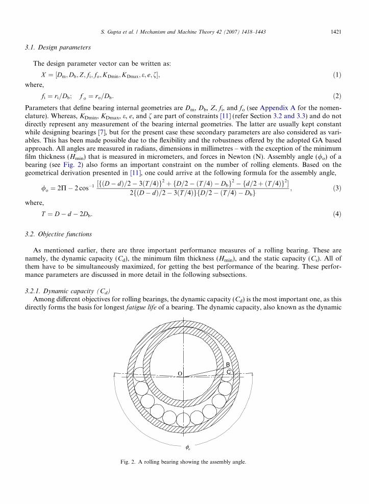
Parameters that define bearing internal geometries are Dm, Db, Z, fi, and fo (see Appendix A for the nomen-clature). Whereas, KDmin, KDmax, e, e, and f are part of constraints [11] (refer Section 3.2 and 3.3) and do notdirectly represent any measurement of the bearing internal geometries. The latter are usually kept constantwhile designing bearings [7], but for the present case these secondary parameters are also considered as vari-ables. This has been made possible due to the flexibility and the robustness offered by the adopted GA basedapproach. All angles are measured in radians, dimensions in millimetres – with the exception of the minimumfilm thickness (Hmin) that is measured in micrometers, and forces in Newton (N). Assembly angle (/o) of abearing (see Fig. 2) also forms an important constraint on the number of rolling elements. Based on thegeometrical derivation presented in [11], one could arrive at the following formula for the assembly angle,
/o ¼ 2P� 2 cos�1 ½fðD� dÞ=2� 3ðT=4Þg2 þ fD=2� ðT =4Þ � Dbg2 � fd=2þ ðT=4Þg2�2fðD� dÞ=2� 3ðT=4ÞgfD=2� ðT =4Þ � Dbg

; ð3Þ

where,

T ¼ D� d � 2Db: ð4Þ

3.2. Objective functions

As mentioned earlier, there are three important performance measures of a rolling bearing. These arenamely, the dynamic capacity (Cd), the minimum film thickness (Hmin), and the static capacity (Cs). All ofthem have to be simultaneously maximized, for getting the best performance of the bearing. These perfor-mance parameters are discussed in more detail in the following subsections.

3.2.1. Dynamic capacity (Cd)

Among different objectives for rolling bearings, the dynamic capacity (Cd) is the most important one, as thisdirectly forms the basis for longest fatigue life of a bearing. The dynamic capacity, also known as the dynamic

O CB

oφ

Fig. 2. A rolling bearing showing the assembly angle.


load rating, is defined as ‘‘the constant radial load, which a group of apparently identical bearings can endurefor a rating life of one million revolutions of the inner ring (for a stationary load and the stationary outerring)’’. It is expressed as [7]:

Cd ¼fcZ2=3D1:8

b Db 6 25:4 mm

3:647f cZ2=3D1:4

b Db > 25:4 mm

(ð5Þ

where,

fc ¼ 37:91 1þ 1:041� c1þ c

� �1:72 fið2f o � 1Þfoð2f i � 1Þ

� �0:41( )10=3

24

35�0:3

c0:3ð1� cÞ1:39

ð1þ cÞ1=3

" #2f i

2f i � 1

� �0:41

ð6Þ

c ¼ Db cos a=Dm: ð7Þ

Here the factor, c, is not an independent parameter. For the current discussion, the deep groove ball bearinghas been considered, for which the contact angle, a, is zero. Therefore, c = Db/Dm. On careful inspection ofEq. (5), it could be observed that the dynamic capacity depends on (2/3)rd to the power of number of rollerand 1.8th to the power the diameter of the ball. Hence, during optimisation, we expect that the maximum pos-sible ball diameter would give us better dynamic capacity. Furthermore, with bigger ball diameter, less numberof balls would be accommodated in a given space. The dynamic capacity is derived on the basis of the max-imum octahedral shear stress that occurs at the subsurface of the contact zone, between trolling elements andraces. Hence, it should be noted that the constraint related to the strength against the shear stress will notappear, explicitly, in constraint section.

3.2.2. Elastohydrodynamic minimum film thickness (Hmin)

Another very important requirement for rolling bearings is the longest wear life. This is directly related tothe minimum film thickness (Hmin) of the lubricant, since it avoids metal-to-metal contact between rolling ele-ments and raceways in rolling bearings. Elastohydrodynamic lubrication (EHL) theory successfully predictsthe minimum film thickness [7]. Considering the requirement of low wear, the optimisation problem aimsat maximizing the minimum film thickness for a given bearing boundary dimensions.

The formula for Hmin is applicable for the inner and outer raceways separately; therefore, for best results,we maximize the lesser of the two. In Eq. (8), the ring can take on values as the inner or outer ring; see usage inEq. (9). The complete objective function, for the minimum film thickness, can thus be given as

H min;ring ¼ 3:63a0:491 R0:466

x;ringE�0:117o Q�0:073 pniDmgoð1� c2Þ

120

� �0:68

1� exp �0:703Rðy;ringÞ

Rðx;ringÞ

� �0:636( )" #

ð8Þ

H min ¼ minðH min;inner;H min;outerÞ ð9Þ

where i represents number of rows. For the present case, a single-row deep groove rolling bearing has beenconsidered and for this i is equal to 1. Sub-expressions used in the final objective function are listed below

Q ¼ 5F r

iZ cos a; ð10Þ

Rðx;innerÞ ¼Db

2ð1� cÞ ; Rðy;innerÞ ¼fiDb

2f i � 1; ð11Þ

Rðx;outerÞ ¼Db

2ð1þ cÞ ; Rðy;outerÞ ¼foDb

2f o � 1: ð12Þ

It should be noted that the nature of Eqs. (8) and (10) is approximate and they should be used with due care.However, a complete load distribution analysis (i.e. finding the maximum load, Q) based on the elastohydro-dynamic lubrication (EHL) integrated approach (i.e. simultaneously obtaining Hmin) is computationally veryexpensive, with the difficulty of inherent convergence problem [7], and not to mention that it is for a singlesolution. The implementation of this analysis, with optimum design, would be very difficult and infeasiblein terms of the computation time, since it would require such analysis of bearing to be performed more than


hundred thousand times (as in the present case). One should also note that these Eqs. (8) and (10) give con-servative estimates of the elastohydrodynamic minimum film thickness and the maximum load.

3.2.3. Static capacity (Cs)

The basic load rating (Cs) (or the static capacity) of a rolling bearing is defined as ‘‘that load applied to anon-rotating bearing that will result in the permanent deformation occurring at the position of the maximumloaded rolling element’’. The static capacity is defined for both the inner as well as the outer raceway. Theobjective function takes the minimum of both values and maximizes that. This approach is similar to theone employed for Hmin.

Cs;inner ¼23:8ZiD2

bða�i b�i Þ3 cos a

4� 1

fi

þ 2c1� c

� �2; Cs;outer ¼

23:8ZiD2bða�ob�oÞ

3 cos a

4� 1

fo

� 2c1þ c

� �2ð13Þ

Cs ¼ minðCs;inner;Cs;outerÞ ð14Þ

The basis of the derivation of the static capacity is the maximum contact stress, which occurs between the roll-ing element and races. Hence, the constraint related to the contact stress will not reflect in the constraint,explicitly.

3.3. Constraints

Constraints reduce the parameter space to the feasible parameter space. This section summarises the nineproblem constraints. Apart from geometrical constraints, we also maintain an intuitive constraint on the num-ber of balls in a given bearing. The first constraint, for the maximum allowance on the assembly angle is [11]

/0

2 sin�1ðDb=DmÞ� Z þ 1 P 0: ð15Þ

This establishes convenience in the bearing assembly and numbers of balls that can be inserted in between theinner and outer raceways. The assembly angle (/o) is found by Eq. (3), which employs important designvariables.

The ball diameter gets an upper and lower bound, through following constraints

2Db � KDminðD� dÞP 0; ð16ÞKDmaxðD� dÞ � 2Db P 0: ð17Þ

Furthermore, an additional constraint, based on the bearing width, which limits the maximum allowablediameter of the ball, is

fBw � Db 6 0: ð18Þ

To guarantee the running mobility of bearings, we must insure that the difference between the pitch diameterand the average diameter in a bearing should be less than a certain value. The inner ring thickness must also bemore than the outer ring thickness, therefore,

Dm � 0:5ðDþ dÞP 0 ð19Þð0:5þ eÞðDþ dÞ � Dm P 0: ð20Þ

The thickness of a bearing ring, at the outer raceway bottom, should not be less than eD, where e is a para-meter obtained from the simple strength consideration of the outer ring. The constraint condition is then

0:5ðD� Dm � DbÞ � eDb P 0: ð21Þ

The groove curvature radii of the inner and outer raceways of a bearing should not be less than 0.515 Db [7],this ensures that the rolling element rolls freely on raceways without any interference. Therefore,

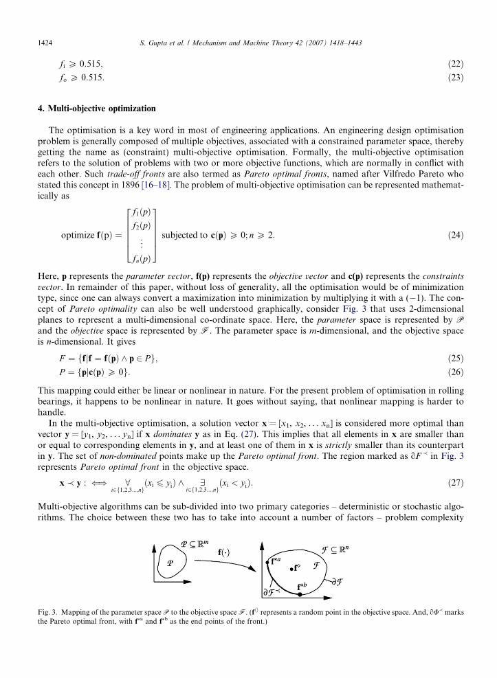
Fig. 3.the Pa


fi P 0:515; ð22Þfo P 0:515: ð23Þ

4. Multi-objective optimization

The optimisation is a key word in most of engineering applications. An engineering design optimisationproblem is generally composed of multiple objectives, associated with a constrained parameter space, therebygetting the name as (constraint) multi-objective optimisation. Formally, the multi-objective optimisationrefers to the solution of problems with two or more objective functions, which are normally in conflict witheach other. Such trade-off fronts are also termed as Pareto optimal fronts, named after Vilfredo Pareto whostated this concept in 1896 [16–18]. The problem of multi-objective optimisation can be represented mathemat-ically as

optimize fðpÞ ¼

f1ðpÞf2ðpÞ

..

.

fnðpÞ

266664

377775 subjected to cðpÞP 0; n P 2: ð24Þ

Here, p represents the parameter vector, f(p) represents the objective vector and c(p) represents the constraints

vector. In remainder of this paper, without loss of generality, all the optimisation would be of minimizationtype, since one can always convert a maximization into minimization by multiplying it with a (�1). The con-cept of Pareto optimality can also be well understood graphically, consider Fig. 3 that uses 2-dimensionalplanes to represent a multi-dimensional co-ordinate space. Here, the parameter space is represented by Pand the objective space is represented by F. The parameter space is m-dimensional, and the objective spaceis n-dimensional. It gives

F ¼ ffjf ¼ fðpÞ ^ p 2 Pg; ð25ÞP ¼ fpjcðpÞP 0g: ð26Þ

This mapping could either be linear or nonlinear in nature. For the present problem of optimisation in rollingbearings, it happens to be nonlinear in nature. It goes without saying, that nonlinear mapping is harder tohandle.

In the multi-objective optimisation, a solution vector x = [x1, x2, . . . xn] is considered more optimal thanvector y = [y1, y2, . . . yn] if x dominates y as in Eq. (27). This implies that all elements in x are smaller thanor equal to corresponding elements in y, and at least one of them in x is strictly smaller than its counterpartin y. The set of non-dominated points make up the Pareto optimal front. The region marked as oF� in Fig. 3represents Pareto optimal front in the objective space.

x � y : () 8i2f1;2;3...;ng

ðxi 6 yiÞ ^ 9i2f1;2;3...;ng

ðxi < yiÞ: ð27Þ

Multi-objective algorithms can be sub-divided into two primary categories – deterministic or stochastic algo-rithms. The choice between these two has to take into account a number of factors – problem complexity

Mapping of the parameter space P to the objective space F. (fhi represents a random point in the objective space. And, oU� marksreto optimal front, with f*a and f*b as the end points of the front.)


(number of objectives and parameters), parameter space (as defined by constraints) and the resources available(time and space). The design of a rolling bearing is a nonlinear multi-objective optimisation problem withmoderate complexity – three objective functions, nine parameters and nine inequality constraints (refer to Sec-tion 3). Deterministic multi-objective optimisation strategies are notorious for getting stuck at local minimaand explode in complexity with the increase in number of parameters. Further, each run of the deterministicalgorithm can provide only single point on the Pareto optimal front. On the other hand, stochastic algorithmseasily dodge local minima, handle parameters more efficiently and a single run of the evolutionary algorithmcan provide numerous non-dominated solution points, thus giving us a close approximation of Pareto optimalfront. In the light of all these factors the evolutionary algorithm for the multi-objective optimisation was cho-sen for application to the current problem.

Over the past decade, a number of multi-objective evolutionary algorithms (MOEAs) have been suggested.The primary reason for this is their ability to find multiple Pareto-optimal solutions in a single run. For prob-lems with a multi-objective formulation, it is not possible to have a single solution, which simultaneously opti-mizes all objectives. In such cases, an algorithm that gives a large number of alternative solutions lying on ornear the Pareto-optimal front is of great practical value. With the growing complexity of engineering prob-lems, popularity of evolutionary algorithms has been on a rise. A good survey and comparison of recent evo-lutionary multi-objective optimisation algorithm can be gathered from [13,14,16–18]. More recently, strength-Pareto EA (SPEA), Pareto-archived evolution strategy (PAES) and NSGA II have gained tremendous pop-ularity for their superior performances. Out of these NSGA II stands out for its fast non-dominated sortingapproach, elitism approach and its overall capability to maintain a better solution spread. Thus being a moti-vation for its use in the design of rolling bearings as presented in this paper. The finer details of this algorithmcan be gathered from [15].

5. Application and results

The work on the design optimisation of rolling bearings is a very active area of research. Some contributionon the design of rolling bearings was made by earlier work of Chakraborty et al. [10] and Rao and Tiwari [11],where GA was used to optimize dynamic capacity for rolling bearings. Results in [10,11] were found to be asmuch as 1.5 times better than those given in standard bearing catalogue [19]. Primary difference between pre-vious works and that presented in this paper is the inclusion of multiple objectives for the simultaneousoptimisation.

5.1. NSGA II implementation and application

NSGA II implementation written by KanGAL, IIT Kanpur [20] was used as the optimisation engine. Awrapper module was written in the C computer language over this optimisation engine, to handle themulti-objective optimisation problem for rolling bearings. The module allows user to specify boundary dimen-sions of the bearing, choose objectives of interest, vary parametric ranges and specify sensitive GA parameters.Real coded chromosomes were used to encode nine design parameters, which are defined in Section 3.1. Prob-lem constraints were incorporated using the standard constraint handling technique [17]. Problem parameterswere given the strict upper and lower bounds (Table 1) to reduce the solution space. Operating conditions arelisted in Table 2, these are same as in [12].

As discussed in Section 3.2, there are three objectives for optimisation – (1) the dynamic capacity Cd, (2) thestatic capacity Cs and (3) the elastohydrodynamic minimum film thickness Hmin. An exhaustive treatment wasgiven to the optimisation problem by choosing all possible combinations of aforementioned objectives. Eachof these combinations was optimised over a broad set of standard bearing boundary dimensions, i.e. the outerdiameter, D, the bore diameter, d and the bearing width Bw. Thus following optimisation runs were made:

• Single objective optimisations: Cd (Table 3), Hmin (Table 4) and Cs (Table 5).• Dual objective optimisations: Cd–Cs (Table 6), Cd–Hmin (Table 7) and Cs–Hmin (Table 8).• Multi-objective optimisation: Cd–Cs–Hmin (Table 9).

Table 1Parametric bounds

Dm � {0.5(D + d), 0.6(D + d)}Db � {0.15(D � d), 0.45(D � d)}Z � (4,50)fi � (0.515,0.6)fo � (0.515,0.6)KDmin � (0.4,0.5)KDmax � (0.6,0.7)e � (0.3,0.4)E � (0.02,0.10)f � (0.6,0.85)

Table 2Operating conditions

a1 = 1e � 08go = 0.02ni = 5000Eo = 2.25e + 11Fr = 15000


A step-by-step procedure for solving the given optimisation problem is illustrated in Fig. 4. The figureassumes understanding of the basic GA terminology. Readers are encouraged to gather more details aboutNSGA II from [15]. The population size, the generation count, the crossover and mutation probabilities weredetermined after multiple runs of the algorithm with the aim of obtaining best solutions. Best here implies themaximum spread of solution points and high values of all the objectives simultaneously. The best results weredecided from a solution set of 20 runs with varying mutation and crossover probabilities, where each GA runused a random seed for generation of the initial population.

The population size was set as 4500 for all the runs, and the convergence was achieved by the end of 50thgeneration for all combinations of the objectives (some combinations converged before 50th generation, butnone after). The value of crossover probability used ranged from 0.7 to 0.85 and the value mutation proba-bility used ranged from 0.15 to 0.2. Although there was no significant impact of variation in these two GAparameters on the obtained solutions, the number of GA generations required for achieving convergenceincreased for values of crossover and mutation probabilities outside this range. The crossover distributionand mutation distribution indices, introduced from the use of real coded chromosomes, were found to bethe most influential NSGA II parameters in the current context. They were assigned values in order to achievethe maximum spread of solution points. Data from multiple runs favoured the crossover distribution index of20, and the mutation distribution index of 10. The lower values of these distribution indices usually gave awider spread to solutions and hence a better approximation of the Pareto-optimal front.

Tables 3–5 give the best optimisation results obtained for the dynamic capacity (Cd), the minimum filmthickness (Hmin) and the static capacity (Cs), respectively. Each of these optimisations is a single objective opti-misation. Table 3 also compares dynamic capacities of optimized bearings with the existing standard [19]. Inorder to compare the increase in the fatigue life of the designed bearings using GAs against the standard val-ues, the relation shown in Eq. (28) has been used. The subscripts d_new and d_std represent the new valuescomputed using GA and those currently available in standards, respectively,

k ¼ Cd new

Cd std

� �3

: ð28Þ

Tables 6–8 show the best results for dual objective optimizations, i.e. dynamic capacity – minimum film thick-ness, dynamic capacity – static capacity and static capacity – minimum film thickness, respectively. These opti-misations are actually the ones that exploited the capability of multi-objective optimisations. The trade-offfront approximation, obtained after every few generation count of NSGA II, was recorded to keep track

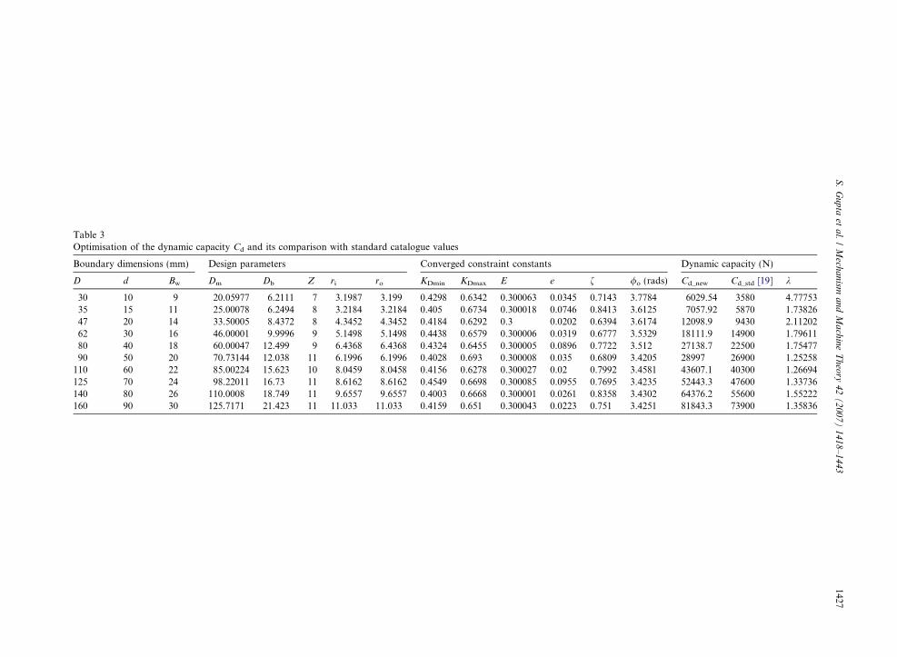
Table 3Optimisation of the dynamic capacity Cd and its comparison with standard catalogue values

Boundary dimensions (mm) Design parameters Converged constraint constants Dynamic capacity (N)

D d Bw Dm Db Z ri ro KDmin KDmax E e f /o (rads) Cd_new Cd_std [19] k

30 10 9 20.05977 6.2111 7 3.1987 3.199 0.4298 0.6342 0.300063 0.0345 0.7143 3.7784 6029.54 3580 4.7775335 15 11 25.00078 6.2494 8 3.2184 3.2184 0.405 0.6734 0.300018 0.0746 0.8413 3.6125 7057.92 5870 1.7382647 20 14 33.50005 8.4372 8 4.3452 4.3452 0.4184 0.6292 0.3 0.0202 0.6394 3.6174 12098.9 9430 2.1120262 30 16 46.00001 9.9996 9 5.1498 5.1498 0.4438 0.6579 0.300006 0.0319 0.6777 3.5329 18111.9 14900 1.7961180 40 18 60.00047 12.499 9 6.4368 6.4368 0.4324 0.6455 0.300005 0.0896 0.7722 3.512 27138.7 22500 1.7547790 50 20 70.73144 12.038 11 6.1996 6.1996 0.4028 0.693 0.300008 0.035 0.6809 3.4205 28997 26900 1.25258

110 60 22 85.00224 15.623 10 8.0459 8.0458 0.4156 0.6278 0.300027 0.02 0.7992 3.4581 43607.1 40300 1.26694125 70 24 98.22011 16.73 11 8.6162 8.6162 0.4549 0.6698 0.300085 0.0955 0.7695 3.4235 52443.3 47600 1.33736140 80 26 110.0008 18.749 11 9.6557 9.6557 0.4003 0.6668 0.300001 0.0261 0.8358 3.4302 64376.2 55600 1.55222160 90 30 125.7171 21.423 11 11.033 11.033 0.4159 0.651 0.300043 0.0223 0.751 3.4251 81843.3 73900 1.35836

S.

Gu

pta

eta

l./

Mech

an

isma

nd

Ma

chin

eT

heo

ry4

2(

20

07

)1

41

8–

14

43

1427

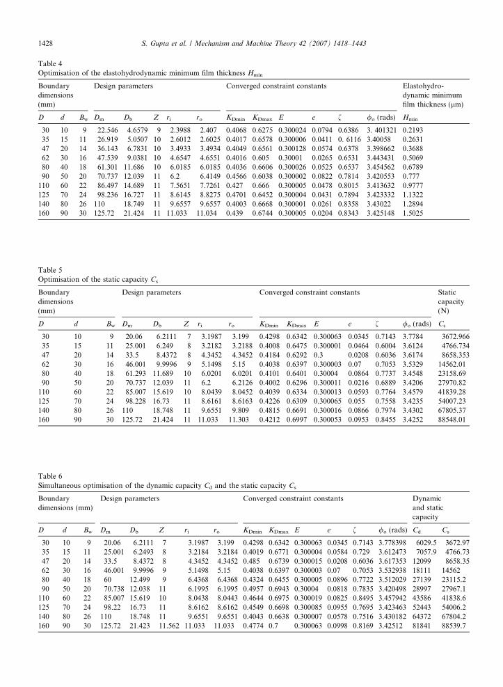
Table 5Optimisation of the static capacity Cs

Boundarydimensions(mm)

Design parameters Converged constraint constants Staticcapacity(N)

D d Bw Dm Db Z ri ro KDmin KDmax E e f /o (rads) Cs

30 10 9 20.06 6.2111 7 3.1987 3.199 0.4298 0.6342 0.300063 0.0345 0.7143 3.7784 3672.96635 15 11 25.001 6.249 8 3.2182 3.2188 0.4008 0.6475 0.300001 0.0464 0.6004 3.6124 4766.73447 20 14 33.5 8.4372 8 4.3452 4.3452 0.4184 0.6292 0.3 0.0208 0.6036 3.6174 8658.35362 30 16 46.001 9.9996 9 5.1498 5.15 0.4038 0.6397 0.300003 0.07 0.7053 3.5329 14562.0180 40 18 61.293 11.689 10 6.0201 6.0201 0.4101 0.6401 0.30004 0.0864 0.7737 3.4548 23158.6990 50 20 70.737 12.039 11 6.2 6.2126 0.4002 0.6296 0.300011 0.0216 0.6889 3.4206 27970.82

110 60 22 85.007 15.619 10 8.0439 8.0452 0.4039 0.6334 0.300013 0.0593 0.7764 3.4579 41839.28125 70 24 98.228 16.73 11 8.6161 8.6163 0.4226 0.6309 0.300065 0.055 0.7558 3.4235 54007.23140 80 26 110 18.748 11 9.6551 9.809 0.4815 0.6691 0.300016 0.0866 0.7974 3.4302 67805.37160 90 30 125.72 21.424 11 11.033 11.303 0.4212 0.6997 0.300053 0.0953 0.8455 3.4252 88548.01

Table 6Simultaneous optimisation of the dynamic capacity Cd and the static capacity Cs

Boundarydimensions (mm)

Design parameters Converged constraint constants Dynamicand staticcapacity

D d Bw Dm Db Z ri ro KDmin KDmax E e f /o (rads) Cd Cs

30 10 9 20.06 6.2111 7 3.1987 3.199 0.4298 0.6342 0.300063 0.0345 0.7143 3.778398 6029.5 3672.9735 15 11 25.001 6.2493 8 3.2184 3.2184 0.4019 0.6771 0.300004 0.0584 0.729 3.612473 7057.9 4766.7347 20 14 33.5 8.4372 8 4.3452 4.3452 0.485 0.6739 0.300015 0.0208 0.6036 3.617353 12099 8658.3562 30 16 46.001 9.9996 9 5.1498 5.15 0.4038 0.6397 0.300003 0.07 0.7053 3.532938 18111 1456280 40 18 60 12.499 9 6.4368 6.4368 0.4324 0.6455 0.300005 0.0896 0.7722 3.512029 27139 23115.290 50 20 70.738 12.038 11 6.1995 6.1995 0.4957 0.6943 0.30004 0.0818 0.7835 3.420498 28997 27967.1

110 60 22 85.007 15.619 10 8.0438 8.0443 0.4644 0.6975 0.300019 0.0825 0.8495 3.457942 43586 41838.6125 70 24 98.22 16.73 11 8.6162 8.6162 0.4549 0.6698 0.300085 0.0955 0.7695 3.423463 52443 54006.2140 80 26 110 18.748 11 9.6551 9.6551 0.4043 0.6638 0.300007 0.0578 0.7516 3.430182 64372 67804.2160 90 30 125.72 21.423 11.562 11.033 11.033 0.4774 0.7 0.300063 0.0998 0.8169 3.42512 81841 88539.7

Table 4Optimisation of the elastohydrodynamic minimum film thickness Hmin


Design parameters Converged constraint constants Elastohydro-dynamic minimumfilm thickness (lm)

D d Bw Dm Db Z ri ro KDmin KDmax E e f /o (rads) Hmin

30 10 9 22.546 4.6579 9 2.3988 2.407 0.4068 0.6275 0.300024 0.0794 0.6386 3. 401321 0.219335 15 11 26.919 5.0507 10 2.6012 2.6025 0.4017 0.6578 0.300006 0.0411 0. 6116 3.40058 0.263147 20 14 36.143 6.7831 10 3.4933 3.4934 0.4049 0.6561 0.300128 0.0574 0.6378 3.398662 0.368862 30 16 47.539 9.0381 10 4.6547 4.6551 0.4016 0.605 0.30001 0.0265 0.6531 3.443431 0.506980 40 18 61.301 11.686 10 6.0185 6.0185 0.4036 0.6606 0.300026 0.0525 0.6537 3.454562 0.678990 50 20 70.737 12.039 11 6.2 6.4149 0.4566 0.6038 0.300002 0.0822 0.7814 3.420553 0.777

110 60 22 86.497 14.689 11 7.5651 7.7261 0.427 0.666 0.300005 0.0478 0.8015 3.413632 0.9777125 70 24 98.236 16.727 11 8.6145 8.8275 0.4701 0.6452 0.300004 0.0431 0.7894 3.423332 1.1322140 80 26 110 18.749 11 9.6557 9.6557 0.4003 0.6668 0.300001 0.0261 0.8358 3.43022 1.2894160 90 30 125.72 21.424 11 11.033 11.034 0.439 0.6744 0.300005 0.0204 0.8343 3.425148 1.5025


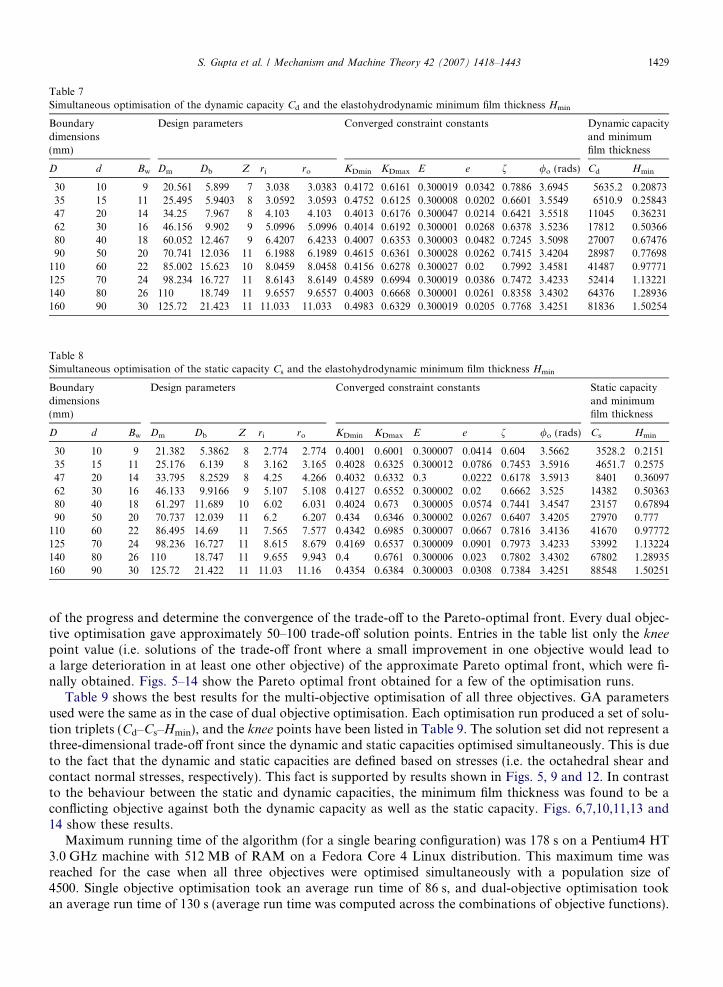
Table 7Simultaneous optimisation of the dynamic capacity Cd and the elastohydrodynamic minimum film thickness Hmin


Design parameters Converged constraint constants Dynamic capacityand minimumfilm thickness

D d Bw Dm Db Z ri ro KDmin KDmax E e f /o (rads) Cd Hmin

30 10 9 20.561 5.899 7 3.038 3.0383 0.4172 0.6161 0.300019 0.0342 0.7886 3.6945 5635.2 0.2087335 15 11 25.495 5.9403 8 3.0592 3.0593 0.4752 0.6125 0.300008 0.0202 0.6601 3.5549 6510.9 0.2584347 20 14 34.25 7.967 8 4.103 4.103 0.4013 0.6176 0.300047 0.0214 0.6421 3.5518 11045 0.3623162 30 16 46.156 9.902 9 5.0996 5.0996 0.4014 0.6192 0.300001 0.0268 0.6378 3.5236 17812 0.5036680 40 18 60.052 12.467 9 6.4207 6.4233 0.4007 0.6353 0.300003 0.0482 0.7245 3.5098 27007 0.6747690 50 20 70.741 12.036 11 6.1988 6.1989 0.4615 0.6361 0.300028 0.0262 0.7415 3.4204 28987 0.77698

110 60 22 85.002 15.623 10 8.0459 8.0458 0.4156 0.6278 0.300027 0.02 0.7992 3.4581 41487 0.97771125 70 24 98.234 16.727 11 8.6143 8.6149 0.4589 0.6994 0.300019 0.0386 0.7472 3.4233 52414 1.13221140 80 26 110 18.749 11 9.6557 9.6557 0.4003 0.6668 0.300001 0.0261 0.8358 3.4302 64376 1.28936160 90 30 125.72 21.423 11 11.033 11.033 0.4983 0.6329 0.300019 0.0205 0.7768 3.4251 81836 1.50254

Table 8Simultaneous optimisation of the static capacity Cs and the elastohydrodynamic minimum film thickness Hmin


Design parameters Converged constraint constants Static capacityand minimumfilm thickness

D d Bw Dm Db Z ri ro KDmin KDmax E e f /o (rads) Cs Hmin

30 10 9 21.382 5.3862 8 2.774 2.774 0.4001 0.6001 0.300007 0.0414 0.604 3.5662 3528.2 0.215135 15 11 25.176 6.139 8 3.162 3.165 0.4028 0.6325 0.300012 0.0786 0.7453 3.5916 4651.7 0.257547 20 14 33.795 8.2529 8 4.25 4.266 0.4032 0.6332 0.3 0.0222 0.6178 3.5913 8401 0.3609762 30 16 46.133 9.9166 9 5.107 5.108 0.4127 0.6552 0.300002 0.02 0.6662 3.525 14382 0.5036380 40 18 61.297 11.689 10 6.02 6.031 0.4024 0.673 0.300005 0.0574 0.7441 3.4547 23157 0.6789490 50 20 70.737 12.039 11 6.2 6.207 0.434 0.6346 0.300002 0.0267 0.6407 3.4205 27970 0.777

110 60 22 86.495 14.69 11 7.565 7.577 0.4342 0.6985 0.300007 0.0667 0.7816 3.4136 41670 0.97772125 70 24 98.236 16.727 11 8.615 8.679 0.4169 0.6537 0.300009 0.0901 0.7973 3.4233 53992 1.13224140 80 26 110 18.747 11 9.655 9.943 0.4 0.6761 0.300006 0.023 0.7802 3.4302 67802 1.28935160 90 30 125.72 21.422 11 11.03 11.16 0.4354 0.6384 0.300003 0.0308 0.7384 3.4251 88548 1.50251


of the progress and determine the convergence of the trade-off to the Pareto-optimal front. Every dual objec-tive optimisation gave approximately 50–100 trade-off solution points. Entries in the table list only the knee

point value (i.e. solutions of the trade-off front where a small improvement in one objective would lead toa large deterioration in at least one other objective) of the approximate Pareto optimal front, which were fi-nally obtained. Figs. 5–14 show the Pareto optimal front obtained for a few of the optimisation runs.

Table 9 shows the best results for the multi-objective optimisation of all three objectives. GA parametersused were the same as in the case of dual objective optimisation. Each optimisation run produced a set of solu-tion triplets (Cd–Cs–Hmin), and the knee points have been listed in Table 9. The solution set did not represent athree-dimensional trade-off front since the dynamic and static capacities optimised simultaneously. This is dueto the fact that the dynamic and static capacities are defined based on stresses (i.e. the octahedral shear andcontact normal stresses, respectively). This fact is supported by results shown in Figs. 5, 9 and 12. In contrastto the behaviour between the static and dynamic capacities, the minimum film thickness was found to be aconflicting objective against both the dynamic capacity as well as the static capacity. Figs. 6,7,10,11,13 and14 show these results.

Maximum running time of the algorithm (for a single bearing configuration) was 178 s on a Pentium4 HT3.0 GHz machine with 512 MB of RAM on a Fedora Core 4 Linux distribution. This maximum time wasreached for the case when all three objectives were optimised simultaneously with a population size of4500. Single objective optimisation took an average run time of 86 s, and dual-objective optimisation tookan average run time of 130 s (average run time was computed across the combinations of objective functions).

Table 9Simultaneous optimisation of the dynamic capacity Cd, the elastohydrodynamic minimum film thickness Hmin and the static capacity Cs

Boundarydimensions (mm)

Design parameters Converged constraint constants Dynamic capacity, minimum filmthickness and static capacity

D d Bw Dm Db Z ri ro KDmin KDmax E e f /o (rads) Cd Hmin Cs

30 10 9 20.702 5.81 7 2.9919 2.9974 0.4046 0.6057 0.300011 0.057 0.693 3.6713 5511.5 0.2096 3401.9135 15 11 25.37 6.017 8 3.099 3.1069 0.4072 0.6461 0.30002 0.0236 0.601 3.569 6630.8 0.2581 4522.0847 20 14 34.131 8.042 8 4.1418 4.1419 0.4005 0.6196 0.300002 0.024 0.604 3.5621 11215 0.362 8103.5262 30 16 46.196 9.876 9 5.0861 5.1361 0.4011 0.6322 0.300027 0.054 0.656 3.5211 17522 0.5037 14292.780 40 18 0.0338 12.48 9 6.4265 6.4273 0.4 0.655 0.300011 0.0234 0.736 3.5106 27060 0.6748 23059.390 50 20 70.739 12.04 11 6.1991 6.1991 0.4089 0.6157 0.300046 0.0306 0.631 3.4205 28993 0.777 27963.9

110 60 22 85.001 15.62 10 8.046 8.1492 0.4027 0.6677 0.300039 0.0591 0.762 3.4581 42691 0.9763 41854.1125 70 24 98.229 16.73 11 8.6166 8.6167 0.4951 0.6362 0.30001 0.0802 0.835 3.4235 52447 1.1323 54012140 80 26 110 18.75 11 9.6557 9.656 0.4014 0.645 0.300007 0.0204 0.748 3.4302 64372 1.2894 67806.5160 90 30 125.72 21.43 11 11.034 11.034 0.4517 0.6511 0.300001 0.0462 0.825 3.4252 81858 1.5026 88558

1430S

.G

up

taet

al.

/M

echa

nism

an

dM

ach

ine

Th

eory

42

(2

00

7)

14

18

–1

44

3

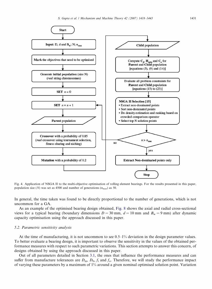
Fig. 4. Application of NSGA II to the multi-objective optimisation of rolling element bearings. For the results presented in this paper,population size (N) was set as 4500 and number of generations (nmax) as 50.


In general, the time taken was found to be directly proportional to the number of generations, which is notuncommon for a GA.

As an example of the optimised bearing design obtained, Fig. 8 shows the axial and radial cross-sectionalviews for a typical bearing (boundary dimensions D = 30 mm, d = 10 mm and Bw = 9 mm) after dynamiccapacity optimisation using the approach discussed in this paper.

5.2. Parametric sensitivity analysis

At the time of manufacturing, it is not uncommon to see 0.5–1% deviation in the design parameter values.To better evaluate a bearing design, it is important to observe the sensitivity in the values of the obtained per-formance measures with respect to such parametric variations. This section attempts to answer this concern, ofdesigns obtained by using the approach discussed in this paper.

Out of all parameters detailed in Section 3.1, the ones that influence the performance measures and cansuffer from manufacture tolerances are Dm, Db, fi and fo. Therefore, we will study the performance impactof varying these parameters by a maximum of 1% around a given nominal optimised solution point. Variation

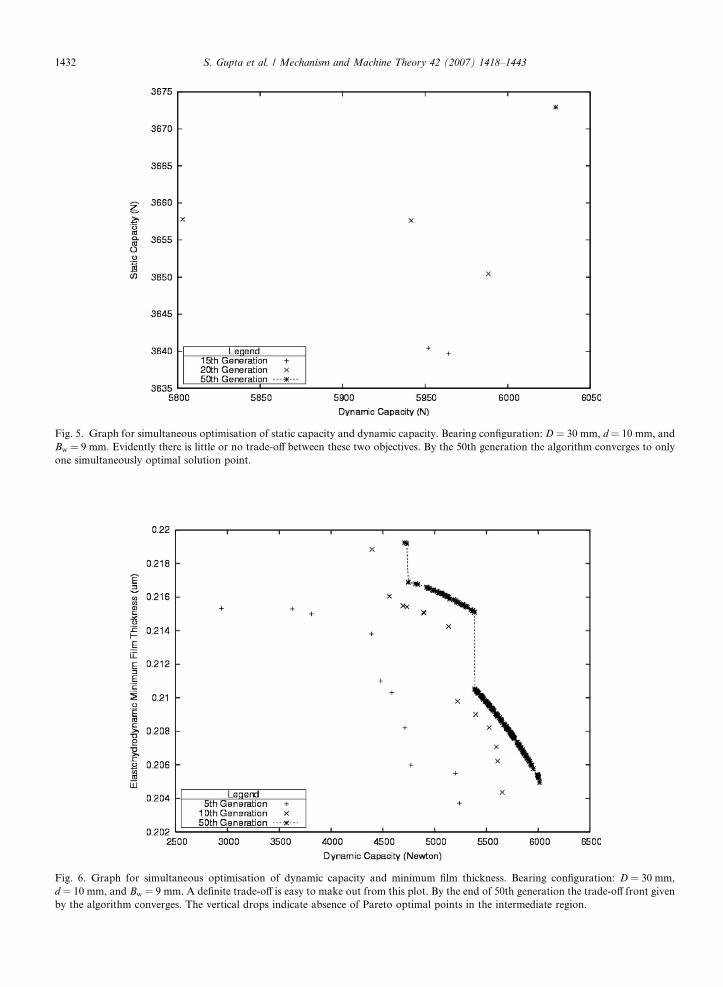
Fig. 5. Graph for simultaneous optimisation of static capacity and dynamic capacity. Bearing configuration: D = 30 mm, d = 10 mm, andBw = 9 mm. Evidently there is little or no trade-off between these two objectives. By the 50th generation the algorithm converges to onlyone simultaneously optimal solution point.

Fig. 6. Graph for simultaneous optimisation of dynamic capacity and minimum film thickness. Bearing configuration: D = 30 mm,d = 10 mm, and Bw = 9 mm. A definite trade-off is easy to make out from this plot. By the end of 50th generation the trade-off front givenby the algorithm converges. The vertical drops indicate absence of Pareto optimal points in the intermediate region.


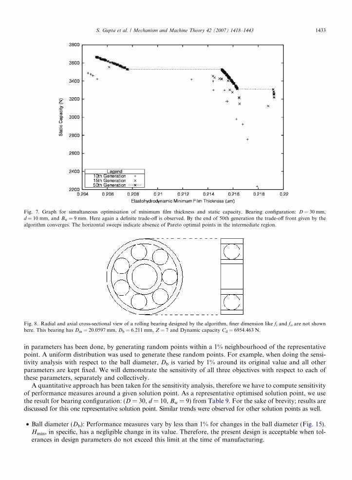
Fig. 7. Graph for simultaneous optimisation of minimum film thickness and static capacity. Bearing configuration: D = 30 mm,d = 10 mm, and Bw = 9 mm. Here again a definite trade-off is observed. By the end of 50th generation the trade-off front given by thealgorithm converges. The horizontal sweeps indicate absence of Pareto optimal points in the intermediate region.

Fig. 8. Radial and axial cross-sectional view of a rolling bearing designed by the algorithm, finer dimension like fi and fo are not shownhere. This bearing has Dm = 20.0597 mm, Db = 6.211 mm, Z = 7 and Dynamic capacity Cd = 6954.463 N.


in parameters has been done, by generating random points within a 1% neighbourhood of the representativepoint. A uniform distribution was used to generate these random points. For example, when doing the sensi-tivity analysis with respect to the ball diameter, Db is varied by 1% around its original value and all otherparameters are kept fixed. We will demonstrate the sensitivity of all three objectives with respect to each ofthese parameters, separately and collectively.

A quantitative approach has been taken for the sensitivity analysis, therefore we have to compute sensitivityof performance measures around a given solution point. As a representative optimised solution point, we usethe result for bearing configuration: (D = 30, d = 10, Bw = 9) from Table 9. For the sake of brevity; results arediscussed for this one representative solution point. Similar trends were observed for other solution points as well.

• Ball diameter (Db): Performance measures vary by less than 1% for changes in the ball diameter (Fig. 15).Hmin, in specific, has a negligible change in its value. Therefore, the present design is acceptable when tol-erances in design parameters do not exceed this limit at the time of manufacturing.

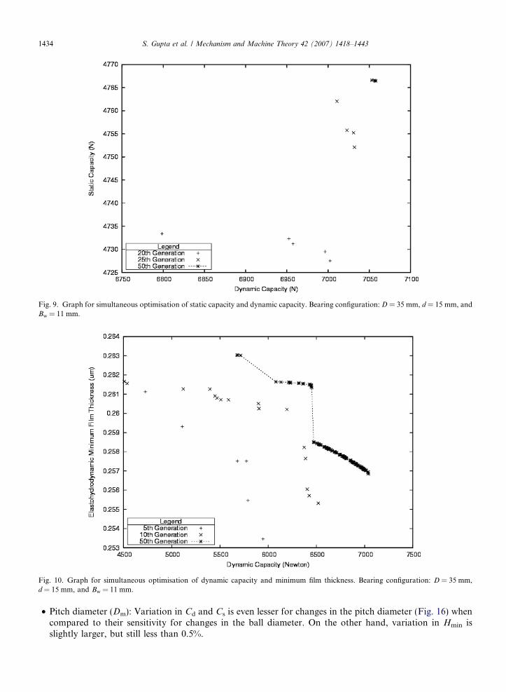
Fig. 9. Graph for simultaneous optimisation of static capacity and dynamic capacity. Bearing configuration: D = 35 mm, d = 15 mm, andBw = 11 mm.

Fig. 10. Graph for simultaneous optimisation of dynamic capacity and minimum film thickness. Bearing configuration: D = 35 mm,d = 15 mm, and Bw = 11 mm.


• Pitch diameter (Dm): Variation in Cd and Cs is even lesser for changes in the pitch diameter (Fig. 16) whencompared to their sensitivity for changes in the ball diameter. On the other hand, variation in Hmin isslightly larger, but still less than 0.5%.

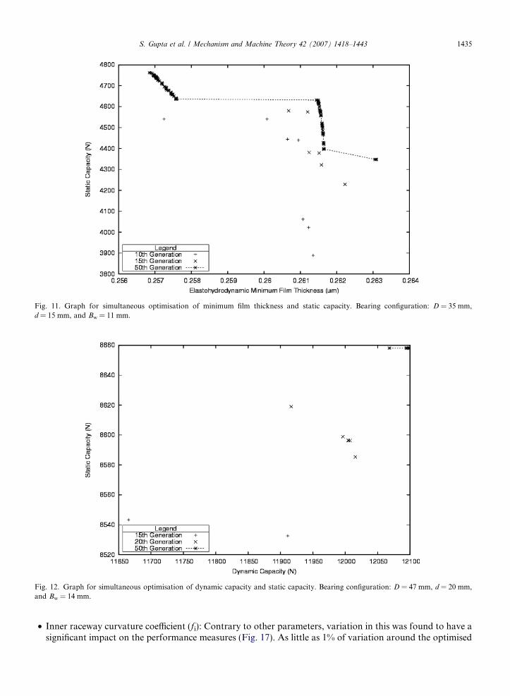
Fig. 11. Graph for simultaneous optimisation of minimum film thickness and static capacity. Bearing configuration: D = 35 mm,d = 15 mm, and Bw = 11 mm.

Fig. 12. Graph for simultaneous optimisation of dynamic capacity and static capacity. Bearing configuration: D = 47 mm, d = 20 mm,and Bw = 14 mm.


• Inner raceway curvature coefficient (fi): Contrary to other parameters, variation in this was found to have asignificant impact on the performance measures (Fig. 17). As little as 1% of variation around the optimised

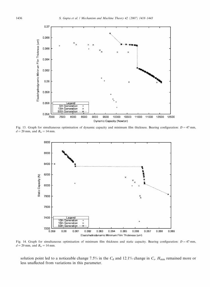
Fig. 13. Graph for simultaneous optimisation of dynamic capacity and minimum film thickness. Bearing configuration: D = 47 mm,d = 20 mm, and Bw = 14 mm.

Fig. 14. Graph for simultaneous optimisation of minimum film thickness and static capacity. Bearing configuration: D = 47 mm,d = 20 mm, and Bw = 14 mm.


solution point led to a noticeable change 7.5% in the Cd and 12.1% change in Cs. Hmin remained more orless unaffected from variations in this parameter.

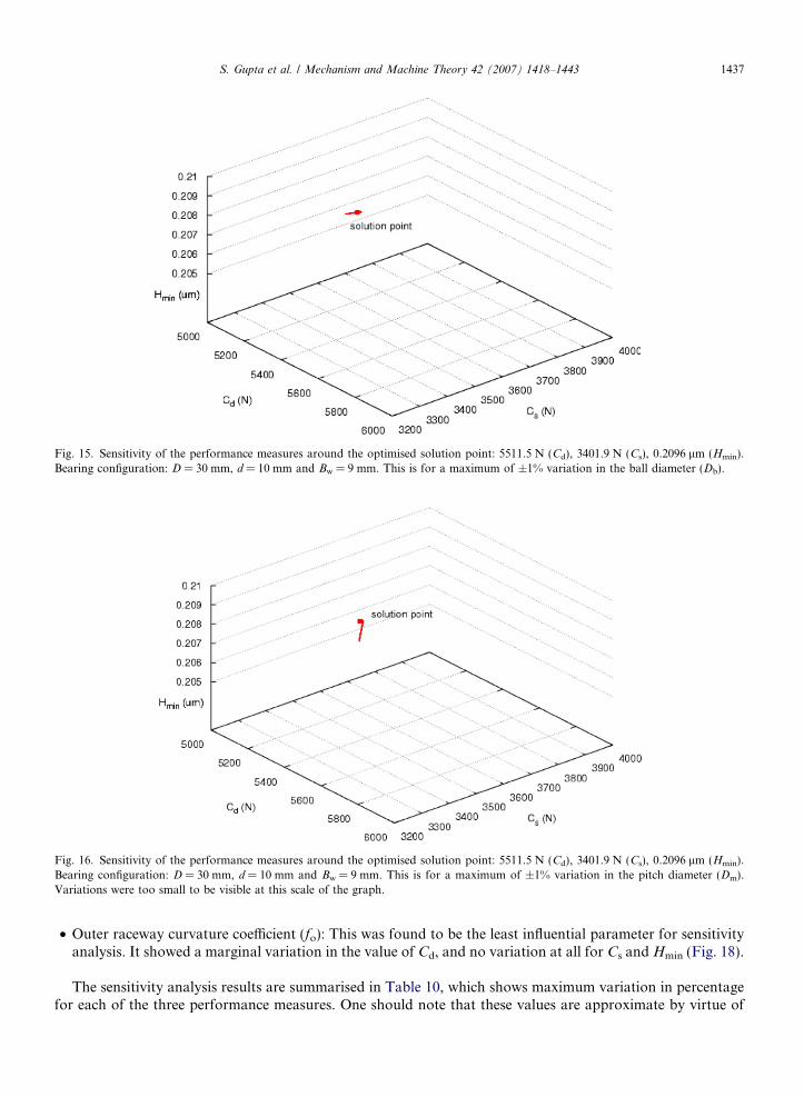
Fig. 15. Sensitivity of the performance measures around the optimised solution point: 5511.5 N (Cd), 3401.9 N (Cs), 0.2096 lm (Hmin).Bearing configuration: D = 30 mm, d = 10 mm and Bw = 9 mm. This is for a maximum of ±1% variation in the ball diameter (Db).

Fig. 16. Sensitivity of the performance measures around the optimised solution point: 5511.5 N (Cd), 3401.9 N (Cs), 0.2096 lm (Hmin).Bearing configuration: D = 30 mm, d = 10 mm and Bw = 9 mm. This is for a maximum of ±1% variation in the pitch diameter (Dm).Variations were too small to be visible at this scale of the graph.


• Outer raceway curvature coefficient (fo): This was found to be the least influential parameter for sensitivityanalysis. It showed a marginal variation in the value of Cd, and no variation at all for Cs and Hmin (Fig. 18).

The sensitivity analysis results are summarised in Table 10, which shows maximum variation in percentagefor each of the three performance measures. One should note that these values are approximate by virtue of

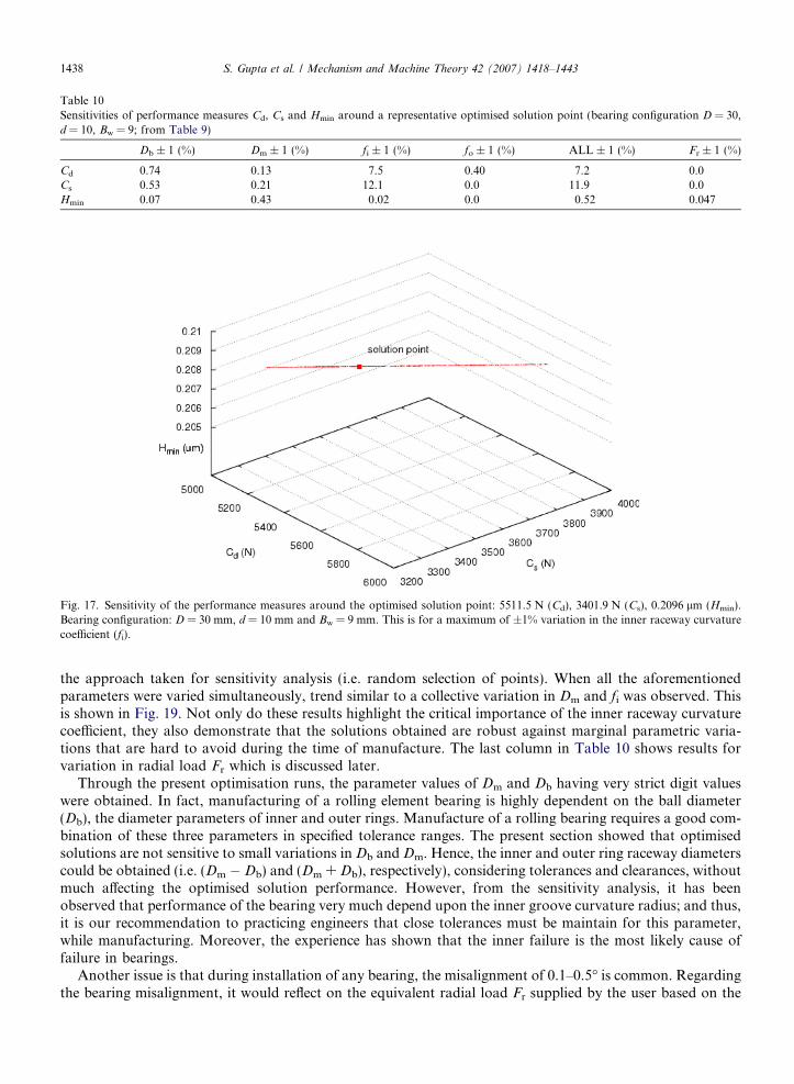
Table 10Sensitivities of performance measures Cd, Cs and Hmin around a representative optimised solution point (bearing configuration D = 30,d = 10, Bw = 9; from Table 9)

Db ± 1 (%) Dm ± 1 (%) fi ± 1 (%) fo ± 1 (%) ALL ± 1 (%) Fr ± 1 (%)

Cd 0.74 0.13 7.5 0.40 7.2 0.0Cs 0.53 0.21 12.1 0.0 11.9 0.0Hmin 0.07 0.43 0.02 0.0 0.52 0.047

Fig. 17. Sensitivity of the performance measures around the optimised solution point: 5511.5 N (Cd), 3401.9 N (Cs), 0.2096 lm (Hmin).Bearing configuration: D = 30 mm, d = 10 mm and Bw = 9 mm. This is for a maximum of ±1% variation in the inner raceway curvaturecoefficient (fi).


the approach taken for sensitivity analysis (i.e. random selection of points). When all the aforementionedparameters were varied simultaneously, trend similar to a collective variation in Dm and fi was observed. Thisis shown in Fig. 19. Not only do these results highlight the critical importance of the inner raceway curvaturecoefficient, they also demonstrate that the solutions obtained are robust against marginal parametric varia-tions that are hard to avoid during the time of manufacture. The last column in Table 10 shows results forvariation in radial load Fr which is discussed later.

Through the present optimisation runs, the parameter values of Dm and Db having very strict digit valueswere obtained. In fact, manufacturing of a rolling element bearing is highly dependent on the ball diameter(Db), the diameter parameters of inner and outer rings. Manufacture of a rolling bearing requires a good com-bination of these three parameters in specified tolerance ranges. The present section showed that optimisedsolutions are not sensitive to small variations in Db and Dm. Hence, the inner and outer ring raceway diameterscould be obtained (i.e. (Dm � Db) and (Dm + Db), respectively), considering tolerances and clearances, withoutmuch affecting the optimised solution performance. However, from the sensitivity analysis, it has beenobserved that performance of the bearing very much depend upon the inner groove curvature radius; and thus,it is our recommendation to practicing engineers that close tolerances must be maintain for this parameter,while manufacturing. Moreover, the experience has shown that the inner failure is the most likely cause offailure in bearings.

Another issue is that during installation of any bearing, the misalignment of 0.1–0.5� is common. Regardingthe bearing misalignment, it would reflect on the equivalent radial load Fr supplied by the user based on the

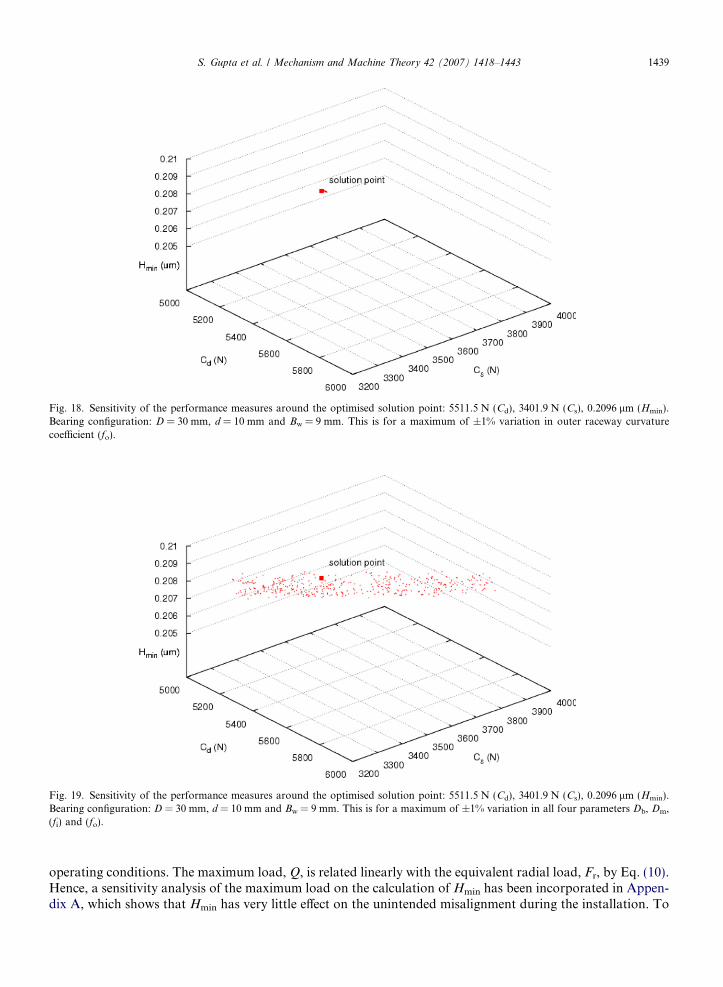
Fig. 19. Sensitivity of the performance measures around the optimised solution point: 5511.5 N (Cd), 3401.9 N (Cs), 0.2096 lm (Hmin).Bearing configuration: D = 30 mm, d = 10 mm and Bw = 9 mm. This is for a maximum of ±1% variation in all four parameters Db, Dm,(fi) and (fo).

Fig. 18. Sensitivity of the performance measures around the optimised solution point: 5511.5 N (Cd), 3401.9 N (Cs), 0.2096 lm (Hmin).Bearing configuration: D = 30 mm, d = 10 mm and Bw = 9 mm. This is for a maximum of ±1% variation in outer raceway curvaturecoefficient (fo).


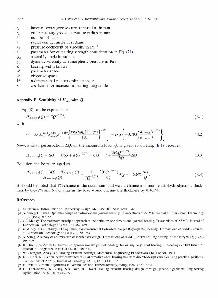
operating conditions. The maximum load, Q, is related linearly with the equivalent radial load, Fr, by Eq. (10).Hence, a sensitivity analysis of the maximum load on the calculation of Hmin has been incorporated in Appen-dix A, which shows that Hmin has very little effect on the unintended misalignment during the installation. To

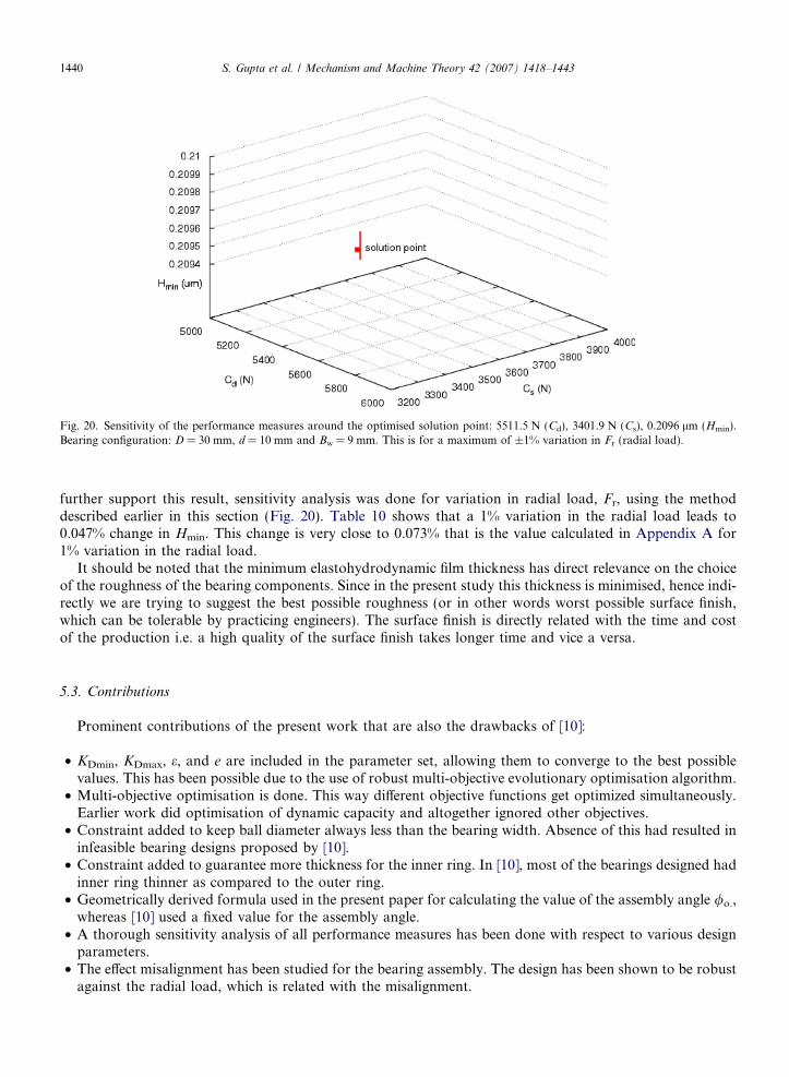
Fig. 20. Sensitivity of the performance measures around the optimised solution point: 5511.5 N (Cd), 3401.9 N (Cs), 0.2096 lm (Hmin).Bearing configuration: D = 30 mm, d = 10 mm and Bw = 9 mm. This is for a maximum of ±1% variation in Fr (radial load).


further support this result, sensitivity analysis was done for variation in radial load, Fr, using the methoddescribed earlier in this section (Fig. 20). Table 10 shows that a 1% variation in the radial load leads to0.047% change in Hmin. This change is very close to 0.073% that is the value calculated in Appendix A for1% variation in the radial load.

It should be noted that the minimum elastohydrodynamic film thickness has direct relevance on the choiceof the roughness of the bearing components. Since in the present study this thickness is minimised, hence indi-rectly we are trying to suggest the best possible roughness (or in other words worst possible surface finish,which can be tolerable by practicing engineers). The surface finish is directly related with the time and costof the production i.e. a high quality of the surface finish takes longer time and vice a versa.

5.3. Contributions

Prominent contributions of the present work that are also the drawbacks of [10]:

• KDmin, KDmax, e, and e are included in the parameter set, allowing them to converge to the best possiblevalues. This has been possible due to the use of robust multi-objective evolutionary optimisation algorithm.

• Multi-objective optimisation is done. This way different objective functions get optimized simultaneously.Earlier work did optimisation of dynamic capacity and altogether ignored other objectives.

• Constraint added to keep ball diameter always less than the bearing width. Absence of this had resulted ininfeasible bearing designs proposed by [10].

• Constraint added to guarantee more thickness for the inner ring. In [10], most of the bearings designed hadinner ring thinner as compared to the outer ring.

• Geometrically derived formula used in the present paper for calculating the value of the assembly angle /o.,whereas [10] used a fixed value for the assembly angle.

• A thorough sensitivity analysis of all performance measures has been done with respect to various designparameters.

• The effect misalignment has been studied for the bearing assembly. The design has been shown to be robustagainst the radial load, which is related with the misalignment.


6. Conclusions

In the present paper, a procedure for the optimisation of rolling bearing design has been proposed. Theoptimisation problem has following characteristics: nonlinear and multi-objectives and subjected to con-straints. Static and dynamic capacities and the elastohydrodynamic minimum thickness have been taken asobjective functions to be maximized. Constraints are mainly kinematics in nature. The NSGA II (non-dom-inated sorting based genetic algorithm) has been applied to the present problem. The following conclusionscan be drawn from the present results:

• The dynamic and static capacities are optimized simultaneously.• Parameters used for constraint equations (KDmin, KDmax, e, e) converge to a very narrow range.• Single trade-off value (per bearing geometry) shown in tables for dual optimisation and triple optimisation

is one among the several trade-off points given by the algorithm. Dual trade-offs can help in efficient designof bearings.

• Trade-off fronts might be used for studying effects of various parameters behind the calculation of dynamicand static capacities of bearings.

• Use of the geometrically accurate formula for / makes calculations useful for real life bearings.• Observation of graphs shows that at the end of each GA generation, algorithm gives out hundreds of trade-

off points.• We can perform parametric study to find out the variation in the trade-off with the changing operating

conditions.• Dynamic and static capacities has been found to be very sensitive to variations in the inner raceway cur-

vature coefficient.

Appendix A

Nomenclature

a�i non-dimensional major axis for the inner raceway contacta�o non-dimensional major axis for the outer raceway contactb�i non-dimensional minor axis for the inner raceway contactb�o non-dimensional minor axis for the outer raceway contactBw bearing width in mmc(p) constraint vectorCd dynamic capacity in NCs static capacity in ND bearing outer diameter in mmDm pitch diameter in mmDb ball diameter in mme parameter for mobility conditions in Eq. (20)Eo equivalent modulus of elasticity in Pafi inner raceway curvature coefficientfo outer raceway curvature coefficientf(p) objective vectorFr radial load in NHmin elastohydrodynamic minimum film thickness in lmi number of rows in the bearingKDmin minimum ball diameter limiterKDmax maximum ball diameter limiterni rotational speed of inner ring in rpmp parameter vector


ri inner raceway groove curvature radius in mmro outer raceway groove curvature radius in mmZ number of ballsa radial contact angle in radiansa1 pressure coefficient of viscosity in Pa�1

e parameter for outer ring strength consideration in Eq. (21)/o assembly angle in radiansgo dynamic viscosity at atmospheric pressure in Pa sZ bearing width limiterP parameter spaceF objective space�1n n-dimensional real co-ordinate spacek coefficient for increase in bearing fatigue life

Appendix B. Sensitivity of Hmin with Q

Eq. (8) can be expressed as

H min;ringðQÞ ¼ CQ�0:073: ðB:1Þ
with
C ¼ 3:63a0:491 R0:466

x;ringE�0:117o

pniDmgoð1� c2Þ120

� �0:68

1� exp �0:703Rðy;ringÞ

Rðx;ringÞ

� �0:636( )" #

: ðB:2Þ

Now, a small perturbation, DQ, on the maximum load, Q, is given, so that Eq. (B.1) becomes

H min;ringðQþ DQÞ ¼ CðQþ DQÞ�0:073 � CQ�0:073 þ oðCQ�0:073ÞoQ

DQ: ðB:3Þ

Equation can be rearranged as

H min;ringðQþ DQÞ � H min;ringðQÞH min;ringðQÞ

¼ 1

CQ�0:073

oðCQ�0:073ÞoQ

DQ ¼ �0:073DQQ: ðB:4Þ

It should be noted that 1% change in the maximum load would change minimum elastohydrodynamic thick-ness by 0.073% and 5% change in the load would change the thickness by 0.365%.

References

[1] M. Asimow, Introduction to Engineering Design, McGraw Hill, New York, 1966.[2] A. Seireg, H. Ezzat, Optimum design of hydrodynamic journal bearings, Transactions of ASME, Journal of Lubrication Technology

91 (3) (1969) 516–523.[3] C.J. Maday, The maximum principle approach to the optimum one-dimensional journal bearing, Transactions of ASME, Journal of

Lubrication Technology 92 (2) (1970) 482–489.[4] G.M. Wylie, C.J. Maday, The optimum one-dimensional hydrodynamic gas Rayleigh step bearing, Transactions of ASME, Journal

of Lubrication Technology 92 (3) (1970) 504–508.[5] A. Seireg, A survey of optimisation of mechanical design, Transactions of ASME, Journal of Engineering for Industry 94 (2) (1972)

495–599.[6] H. Hirani, K. Athre, S. Biswas, Comprehensive design methodology for an engine journal bearing, Proceedings of Institution of

Mechanical Engineers, Part J 214 (2000) 401–412.[7] W. Changsen, Analysis of Rolling Element Bearings, Mechanical Engineering Publications Ltd, London, 1991.[8] D.H. Choi, K.C. Yoon, A design method of an automotive wheel bearing unit with discrete design variables using genetic algorithms,

Transactions of ASME, Journal of Tribology 123 (1) (2001) 181–187.[9] P. Periaux, Genetic Algorithms in Aeronautics and Turbomachinery, Wiley, New York, 2002.

[10] I. Chakraborthy, K. Vinay, S.B. Nair, R. Tiwari, Rolling element bearing design through genetic algorithms, EngineeringOptimisation 35 (6) (2003) 649–659.


[11] B.R. Rao, R. Tiwari, Optimum design of rolling element bearings using genetic algorithms, Mechanism and Machine Theory 42 (2)(2007) 233–250.

[12] K. Kalita, R. Tiwari, S.K. Kakoty, Multi-Objective Optimisation in rolling element bearing system design, in: Proceedings of theInternational Conference on Optimisation SIGOPT 2002, February 17–22, Lambrecht, Germany, 2002.

[13] C.C.A. Coello, Handling Preferences in Evolutionary Multi-Objective Optimisation: A Survey. Congress on EvolutionaryComputation, vol. 1, IEEE Service Center, Piscataway, NJ, Julio del 2000, 2000, pp. 30–37.

[14] E. Zitzler, Evolutionary Algorithms for Multi-objective Optimisation: Methods and Application, Ph.D. thesis, Swiss Federal Instituteof Technology (ETH), Aachen, Germany, 1999.

[15] K. Deb, S. Agrawal, A. Pratap, T. Meyarivan, A fast elitist non-dominated sorting genetic algorithm for multi-objective optimisation:NSGA-II, in: Proceedings of the Parallel Problem Solving from Nature VI Conference, Paris, France, Lecture Notes in ComputerScience No. 1917, Springer, 2000, pp. 849–858.

[16] K. Miettinen, Nonlinear Multi-objective Optimisation, Kluwer Academic Publishers, Boston, 1999.[17] K. Deb, Multi-objective Optimisation Using Evolutionary Algorithms, Wiley–Interscience Series in Systems and Optimisation,

New York, 2001.[18] J. Andersson, Multi-objective Optimisation in Engineering Design: Applications to Fluid Power Systems, Ph.D. Thesis, Division of

Fluid and Mechanical Engineering Systems, Department of Mechanical Engineering, Linkopings University, Sweden, 2001.[19] J.E. Shigley, C.R. Mischke, Mechanical Engineering Design, McGraw-Hill Book Company, New York, 1989.[20] KanGAL (Kanpur Genetic Algorithm Laboratory), Indian Institute of Technology Kanpur, India. http://www.iitk.ac.in/kangal/.

http://www.iitk.ac.in/kangal/

Documents

Multi-objective design optimisation of rolling …web.eecs.umich.edu/~shangupt/publications/sgupta-mamt07.pdf · Multi-objective design optimisation of rolling bearings ... Only the