Embed Size (px)
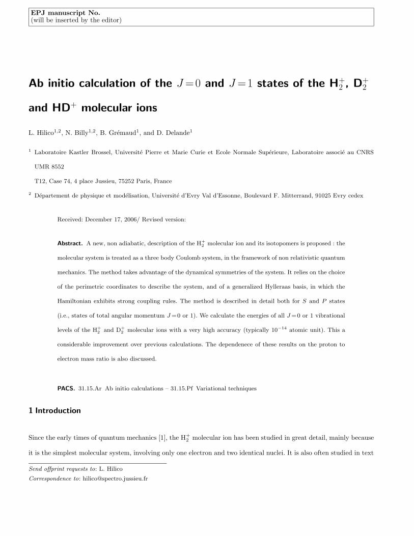
Citation preview

HAL Id: hal-00120666https://hal.archives-ouvertes.fr/hal-00120666
Submitted on 17 Dec 2006
HAL is a multi-disciplinary open accessarchive for the deposit and dissemination of sci-entific research documents, whether they are pub-lished or not. The documents may come fromteaching and research institutions in France orabroad, or from public or private research centers.
L’archive ouverte pluridisciplinaire HAL, estdestinée au dépôt et à la diffusion de documentsscientifiques de niveau recherche, publiés ou non,émanant des établissements d’enseignement et derecherche français ou étrangers, des laboratoirespublics ou privés.
Ab initio calculation of the J=0 and J=1 states of theH2+, D2+ and HD+ molecular ions
Laurent Hilico, Nicolas Billy, Benoît Grémaud, Dominique Delande
To cite this version:Laurent Hilico, Nicolas Billy, Benoît Grémaud, Dominique Delande. Ab initio calculation of the J=0and J=1 states of the H2+, D2+ and HD+ molecular ions. European Physical Journal A, EDPSciences, 2000, 12, pp.449. �hal-00120666�
EPJ manuscript No.(will be inserted by the editor)
Ab initio calculation of the J =0 and J =1 states of the H+2 , D+
2
and HD+ molecular ions
L. Hilico1,2, N. Billy1,2, B. Gremaud1, and D. Delande1
1 Laboratoire Kastler Brossel, Universite Pierre et Marie Curie et Ecole Normale Superieure, Laboratoire associe au CNRS
UMR 8552
T12, Case 74, 4 place Jussieu, 75252 Paris, France
2 Departement de physique et modelisation, Universite d’Evry Val d’Essonne, Boulevard F. Mitterrand, 91025 Evry cedex
Received: December 17, 2006/ Revised version:
Abstract. A new, non adiabatic, description of the H+
2 molecular ion and its isotopomers is proposed : the
molecular system is treated as a three body Coulomb system, in the framework of non relativistic quantum
mechanics. The method takes advantage of the dynamical symmetries of the system. It relies on the choice
of the perimetric coordinates to describe the system, and of a generalized Hylleraas basis, in which the
Hamiltonian exhibits strong coupling rules. The method is described in detail both for S and P states
(i.e., states of total angular momentum J =0 or 1). We calculate the energies of all J =0 or 1 vibrational
levels of the H+
2 and D+
2 molecular ions with a very high accuracy (typically 10−14 atomic unit). This a
considerable improvement over previous calculations. The dependenece of these results on the proton to
electron mass ratio is also discussed.
PACS. 31.15.Ar Ab initio calculations – 31.15.Pf Variational techniques
1 Introduction
Since the early times of quantum mechanics [1], the H+2 molecular ion has been studied in great detail, mainly because
it is the simplest molecular system, involving only one electron and two identical nuclei. It is also often studied in text
Send offprint requests to: L. Hilico
Correspondence to: [email protected]
2 L. Hilico et al.: Ab initio calculation of the J =0 and J =1 states of the H+
2 , D+
2 and HD+ molecular ions
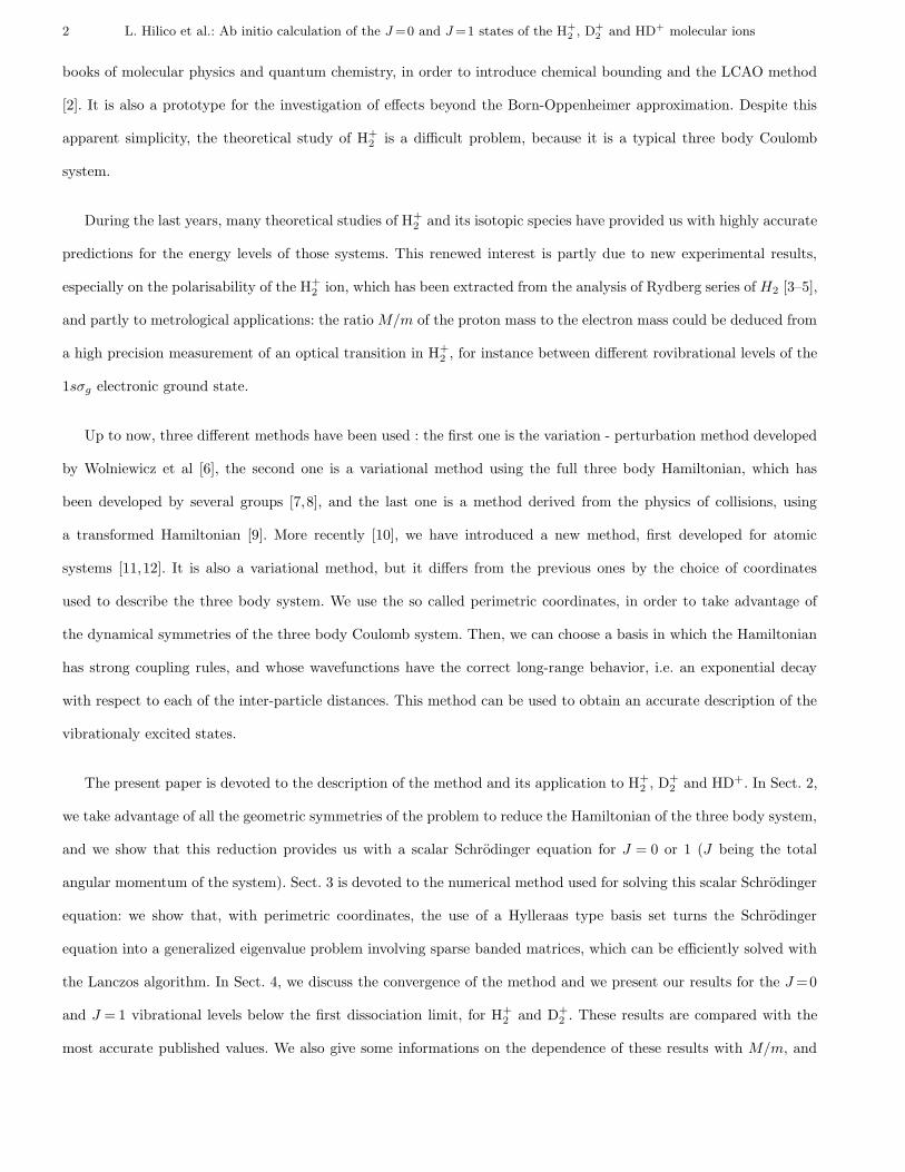
books of molecular physics and quantum chemistry, in order to introduce chemical bounding and the LCAO method
[2]. It is also a prototype for the investigation of effects beyond the Born-Oppenheimer approximation. Despite this
apparent simplicity, the theoretical study of H+2 is a difficult problem, because it is a typical three body Coulomb
system.
During the last years, many theoretical studies of H+2 and its isotopic species have provided us with highly accurate
predictions for the energy levels of those systems. This renewed interest is partly due to new experimental results,
especially on the polarisability of the H+2 ion, which has been extracted from the analysis of Rydberg series of H2 [3–5],
and partly to metrological applications: the ratio M/m of the proton mass to the electron mass could be deduced from
a high precision measurement of an optical transition in H+2 , for instance between different rovibrational levels of the
1sσg electronic ground state.
Up to now, three different methods have been used : the first one is the variation - perturbation method developed
by Wolniewicz et al [6], the second one is a variational method using the full three body Hamiltonian, which has
been developed by several groups [7,8], and the last one is a method derived from the physics of collisions, using
a transformed Hamiltonian [9]. More recently [10], we have introduced a new method, first developed for atomic
systems [11,12]. It is also a variational method, but it differs from the previous ones by the choice of coordinates
used to describe the three body system. We use the so called perimetric coordinates, in order to take advantage of
the dynamical symmetries of the three body Coulomb system. Then, we can choose a basis in which the Hamiltonian
has strong coupling rules, and whose wavefunctions have the correct long-range behavior, i.e. an exponential decay
with respect to each of the inter-particle distances. This method can be used to obtain an accurate description of the
vibrationaly excited states.
The present paper is devoted to the description of the method and its application to H+2 , D+
2 and HD+. In Sect. 2,
we take advantage of all the geometric symmetries of the problem to reduce the Hamiltonian of the three body system,
and we show that this reduction provides us with a scalar Schrodinger equation for J = 0 or 1 (J being the total
angular momentum of the system). Sect. 3 is devoted to the numerical method used for solving this scalar Schrodinger
equation: we show that, with perimetric coordinates, the use of a Hylleraas type basis set turns the Schrodinger
equation into a generalized eigenvalue problem involving sparse banded matrices, which can be efficiently solved with
the Lanczos algorithm. In Sect. 4, we discuss the convergence of the method and we present our results for the J=0
and J = 1 vibrational levels below the first dissociation limit, for H+2 and D+
2 . These results are compared with the
most accurate published values. We also give some informations on the dependence of these results with M/m, and
L. Hilico et al.: Ab initio calculation of the J =0 and J =1 states of the H+
2 , D+
2 and HD+ molecular ions 3
we discuss the interest of a high resolution spectroscopy measurement in H+2 . Finally, the energies of the J=0 states
of HD+ are given in Sect. 5.
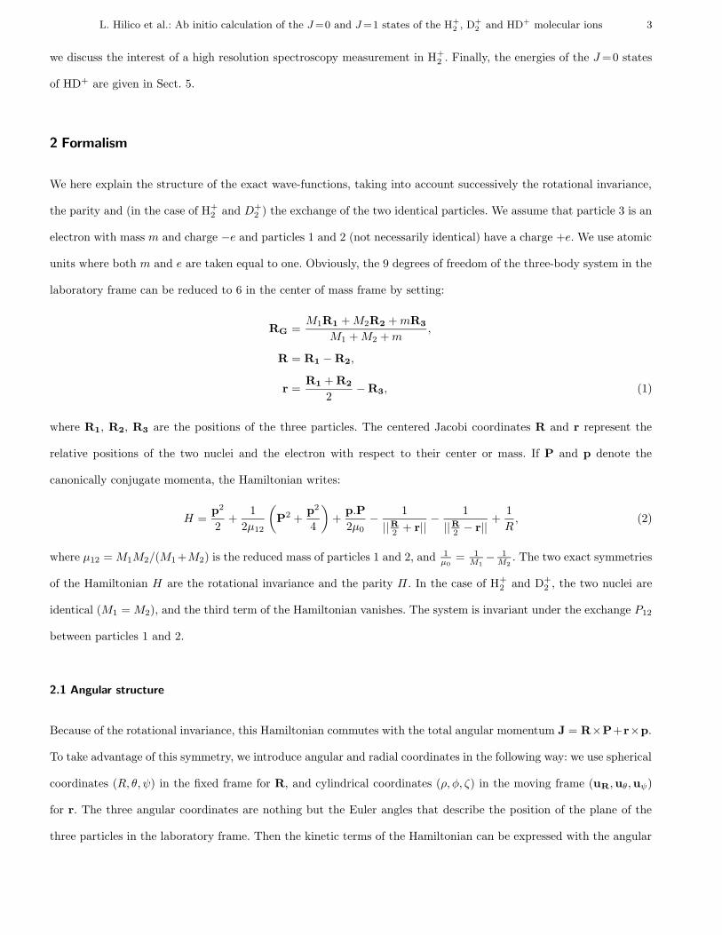
2 Formalism
We here explain the structure of the exact wave-functions, taking into account successively the rotational invariance,
the parity and (in the case of H+2 and D+
2 ) the exchange of the two identical particles. We assume that particle 3 is an
electron with mass m and charge −e and particles 1 and 2 (not necessarily identical) have a charge +e. We use atomic
units where both m and e are taken equal to one. Obviously, the 9 degrees of freedom of the three-body system in the
laboratory frame can be reduced to 6 in the center of mass frame by setting:
RG =M1R1 +M2R2 +mR3
M1 +M2 +m,
R = R1 − R2,
r =R1 + R2
2− R3, (1)
where R1, R2, R3 are the positions of the three particles. The centered Jacobi coordinates R and r represent the
relative positions of the two nuclei and the electron with respect to their center or mass. If P and p denote the
canonically conjugate momenta, the Hamiltonian writes:
H =p2
2+
1
2µ12
(P2 +
p2
4
)+
p.P
2µ0− 1
||R2 + r||− 1
||R2 − r||+
1
R, (2)
where µ12 = M1M2/(M1 +M2) is the reduced mass of particles 1 and 2, and 1µ0
= 1M1
− 1M2
. The two exact symmetries
of the Hamiltonian H are the rotational invariance and the parity Π. In the case of H+2 and D+
2 , the two nuclei are
identical (M1 = M2), and the third term of the Hamiltonian vanishes. The system is invariant under the exchange P12
between particles 1 and 2.
2.1 Angular structure
Because of the rotational invariance, this Hamiltonian commutes with the total angular momentum J = R×P+r×p.
To take advantage of this symmetry, we introduce angular and radial coordinates in the following way: we use spherical
coordinates (R, θ, ψ) in the fixed frame for R, and cylindrical coordinates (ρ, φ, ζ) in the moving frame (uR,uθ,uψ)
for r. The three angular coordinates are nothing but the Euler angles that describe the position of the plane of the
three particles in the laboratory frame. Then the kinetic terms of the Hamiltonian can be expressed with the angular
4 L. Hilico et al.: Ab initio calculation of the J =0 and J =1 states of the H+
2 , D+
2 and HD+ molecular ions
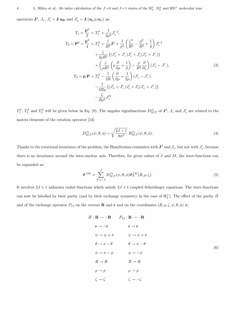
operators J2, Jz, J′z = J.uR and J ′
± = J.(uρ±iuφ) as:
T1 =p2
2= TS1 +
1
2ρ2J ′ 2z ,
T2 = P2 +p2
4= TS2 +
1
R2J2 +
1
ρ2
(ζ2
R2− ρ2
R2+
1
4
)J ′ 2z
+ζ
2ρR2
((J ′
+ + J ′−)J ′
z + J ′z(J
′+ + J ′
−))
+
(ζ
ρR2
(ρ∂
∂ρ+
1
2
)− ρ
R2
∂
∂ζ
)(J ′
+ − J ′−), (3)
T3 = p.P = TS3 − 1
2R
(∂
∂ρ+
1
2ρ
)(J ′
+ − J ′−)
− 1
4Rρ
((J ′
+ + J ′−)J ′
z + J ′z(J
′+ + J ′
−))
− ζ
Rρ2J ′2z .
TS1 , TS2 and TS3 will be given below in Eq. (9). The angular eigenfunctions DJ∗M,T of J2, Jz and J ′
z are related to the
matrix elements of the rotation operator [13]:
DJ∗M,T (ψ, θ, φ) =
√2J + 1
8π2RJ∗M,T (ψ, θ, φ). (4)
Thanks to the rotational invariance of the problem, the Hamiltonian commutes with J2 and Jz , but not with J ′z, because
there is no invariance around the inter-nuclear axis. Therefore, for given values of J and M , the wave-functions can
be expanded as:
ΨJM =
J∑
T=−J
DJ∗M,T (ψ, θ, φ)ΦJMT (R, ρ, ζ). (5)
It involves 2J + 1 unknown radial functions which satisfy 2J + 1 coupled Schrodinger equations. The wave-functions
can now be labelled by their parity (and by their exchange symmetry in the case of H+2 ). The effect of the parity Π
and of the exchange operator P12 on the vectors R and r and on the coordinates (R, ρ, ζ, ψ, θ, φ) is:
Π : R → −R P12 : R → −R
r → −r r → r
ψ → ψ + π ψ → ψ + π
θ → π − θ θ → π − θ
φ→ π − φ φ→ −φ
R→ R R→ R
ρ→ ρ ρ→ ρ
ζ → ζ ζ → −ζ
(6)
L. Hilico et al.: Ab initio calculation of the J =0 and J =1 states of the H+
2 , D+
2 and HD+ molecular ions 5
The symmetry properties of the DJ∗M,T functions with respect to Π and P12 are:
Π DJ∗M,T (ψ, θ, φ) = (−1)J+TDJ∗
M,−T (ψ, θ, φ), (7)
P12 DJ∗M,T (ψ, θ, φ) = (−1)JDJ∗
M,−T (ψ, θ, φ). (8)
We now succesively study the simplest cases, namely the J=0 and J=1 states and show how to solve the 2J + 1
coupled differential equations.
2.1.1 S states
The S states, corresponding to J = M = T = 0, are even states because the angular dependence reduces to a constant
1/√
8π2. There is a single term in the expansion , Eq. (5). Thus, the energy levels are determined by a scalar radial
Schrodinger equation with the effective Hamiltonian HS = TS1 + 12µ12
TS2 + 12µ0
TS3 + V where TS1 , TS2 and TS3 are the
terms of Eq. (3) that do not depend on the angular momentum. The three kinetic terms of the Hamiltonian as well
as the potential energy are:
TS1 = −1
2
(∂2
∂ρ2+
1
ρ
∂
∂ρ+
∂2
∂ζ2
),
TS2 = − ∂2
∂R2− 2
R
∂
∂R−(ζ2
R2+
1
4
)∂2
∂ρ2−(ρ2
R2+
1
4
)∂2
∂ζ2
−(ζ2
R2− ρ2
R2+
1
4
)1
ρ
∂
∂ρ+ 2
ζ
R2
∂
∂ζ+ 2
ρζ
R2
∂2
∂ρ∂ζ, (9)
TS3 = −(
∂2
∂R∂ζ− ζ
R
∂2
∂ρ2+ρ
R
∂2
∂ρ∂ζ− ζ
Rρ
∂
∂ρ+
2
R
∂
∂ζ
),
V = −1/
√(ζ +
R
2
)2
+ ρ2 − 1/
√(ζ − R
2
)2
+ ρ2 +1
R.
2.1.2 The P states
The P states correspond to J = 1. For each M value, the expansion of the wave-function in Eq. (5) involves three
unknown radial functions. Because of the symmetry of the Hamiltonian with respect to the parity Π, we can describe
the even and odd states separately. Since the parity only affects the angular dependence of the wave-functions, it is
useful to introduce one even and two odd angular functions on which the wave-functions may be expanded.
Even P states are very similar to S states, because there is a single even angular function (D1∗M,1 +D1∗
M,−1)/√
2, so
that an even P wave-function simply writes:
Ψ1Me =
(D1∗M,1 +D1∗
M,−1)√2
Rρ Φ1Me (R, ρ, ζ). (10)

6 L. Hilico et al.: Ab initio calculation of the J =0 and J =1 states of the H+
2 , D+
2 and HD+ molecular ions
After multiplying the Schrodinger equation by Rρ, the radial function Φ1Me obeys the scalar generalized Schrodinger
equation:
HP e
Φ1Me = E R2 ρ2 Φ1M
e , (11)
involving the effective Hamiltonian HP e
= TPe
1 + 12µ12
TPe
2 + 12µ0
TPe
3 + V Pe
where:
TPe
1 = R2ρ2 TS1 −R2 ρ∂
∂ρ,
TPe
2 = R2ρ2 TS2 +R ρ
(−2ρ
∂
∂R− 2R
(ζ2
R2+
1
4
)∂
∂ρ+
2ρζ
R
∂
∂ζ
), (12)
TPe
3 = R2ρ2 TS3 +R ρ
(2ζ
∂
∂ρ− 2ρ
∂
∂ζ
),
V Pe
= R2ρ2 V.
The Rρ factor is introduced in Eq. (10) in order to regularize the terms of the Hamiltonian depending on the angular
momentum.
For odd P states, the situation is slightly more complicated. Indeed, the expansion in Eq. (5) can be reduced to
two terms associated with the two odd angular functions:
Ψ1Mo = D1∗
M,0 Φ0(R, ρ, ζ) +
D1∗M,−1 −D1∗
M,1√2
Φ1(R, ρ, ζ). (13)
In the angular basis {D1∗M,0, (D
1∗M,−1 − D1∗
M,1)/√
2}, the angular operators involved in Eq. (3) are represented by the
matrices:
J2 =
2 0
0 2
, J ′
+ − J ′− =
0 −2
2 0
, J ′ 2
z =
0 0
0 1
,
(J ′+ + J ′
−)J ′z + J ′
z(J′+ + J ′
−) =
0 −2
−2 0
.
The two radial wave-functions Φ0 and Φ1 obey the two following coupled Schrodinger equations:
HP o
Φ0
Φ1
= E
Φ0
Φ1
, (14)
where HP o
is a 2x2 matrix of differential operators that can be easily deduced from Eq. (3). Again, in order to
regularize the terms of the Hamiltonian depending on the angular momentum, we follow Wintgen and Delande [14]
who proposed to introduce the two radial functions F and G defined by:
Φ0
Φ1
= M
F
G
with M =
ζ + R
2 ζ − R2
ρ ρ
. (15)
L. Hilico et al.: Ab initio calculation of the J =0 and J =1 states of the H+
2 , D+
2 and HD+ molecular ions 7
F and G are the solutions of the two coupled Schrodinger equations:
HP o
F
G
= EP
o
F
G
(16)
with HP o
= M† HP o
M and EPo
= E M † M . The four contributions to HP o
= TPo
1 + 12µ12
TPo
2 + 12µ0
TPo
3 + V Po
can
be written as:
TPo
1 =
T dir1 T exch1
T exch1 T dir1
,
TPo
2 =
T dir2 T exch2
T exch2 T dir2
, (17)
TPo
3 =
T dir3 T exch3
−T exch3 −T dir3
,
V Po
= M†M V S .
In the previous equations, the ˜ operation is associated with the change ζ → −ζ, i.e., for a radial function f , we set
f(R, ρ, ζ) = f(R, ρ,−ζ), and, for an operator T , we set T (R, ρ, ζ, ∂∂R ,
∂∂ρ ,
∂∂ζ ) = T (R, ρ,−ζ, ∂
∂R ,∂∂ρ ,− ∂
∂ζ ).
The operators appearing in Eq. (17) are:
T dir1 =
((ζ +
R
2
)2
+ ρ2
)TS1 − ρ
∂
∂ρ−(ζ +
R
2
)∂
∂ζ,
T exch1 =
(ζ2 − R2
4+ ρ2
)TS1 − ρ
∂
∂ρ−(ζ +
R
2
)∂
∂ζ,
T dir2 =
((ζ +
R
2
)2
+ ρ2
)TS2
−(ζ +
R
2
)∂
∂R+
(ζ
R− 1
2
)ρ∂
∂ρ− 1
2
(ζ +
R
2+ 2
ρ2
R
)∂
∂ζ,
T exch2 =
(ζ2 − R2
4+ ρ2
)TS2
+
(ζ +
R
2
)∂
∂R−(ζ
R+
1
2
)ρ∂
∂ρ− 1
2
(ζ +
R
2− 2
ρ2
R
)∂
∂ζ,
T dir3 =
((ζ +
R
2)2 + ρ2
)TS3
8 L. Hilico et al.: Ab initio calculation of the J =0 and J =1 states of the H+
2 , D+
2 and HD+ molecular ions
−(ζ +
R
2
)∂
∂R+
(ζ
R− 1
2
)ρ∂
∂ρ− 1
2
(ζ +
R
2+ 2
ρ2
R
)∂
∂ζ,
T exch3 =
(ζ2 − R2
4+ ρ2
)TS3
−(ζ +
R
2
)∂
∂R+
(ζ
R+
1
2
)ρ∂
∂ρ+
1
2
(ζ +
R
2− 2
ρ2
R
)∂
∂ζ,
and M†M =
(ζ + R
2
)2+ ρ2 ζ2 − R2
4 + ρ2
ζ2 − R2
4 + ρ2(ζ − R
2
)2+ ρ2
.
The radial factorizations introduced in Eqs. (10), (13) and (15) can be understood from the following argument: the
formalism used here was first developed to describe an Helium atom (particles 1 and 2 become electrons and particle
3 is the nucleus)[14]. For an infinitely massive electron, and if the Coulomb interaction between the two electrons is
neglected, the Hamiltonian becomes H = p12
2 + p22
2 − 2r1
− 2r2
. The exact solutions of this three body problem are
products of hydrogenic wave functions in r1 and r2. Studying the structure of those solutions [15,16] that correspond
to either P e or P o states shows that it is always possible to factorize them as indicated.
So far, we have taken into account only the rotational and parity symmetries to derive the structure of the J =0
and J=1 wave-functions. The result stands for any potential energy V depending only on the inter-particle distances.
2.2 Exchange symmetry
In the case of H+2 , we have an additional symmetry corresponding to the exchange of the two protons. The T3
contribution to the Hamiltonian disappears since 1µ0
vanishes. The Hamiltonian then commutes with the exchange
operator P12: the wave functions are either symmetric or antisymmetric with respect to P12. Like in the atomic case,
we will note here spatially symmetric (respectively antisymmetric) states as singlets (resp. triplets). Alternatively,
they can be labelled para (resp. ortho). For J=0, we thus have singlet 1Se and triplet 3Se states. For J=1, the total
parity can be either even or odd, thus producing 1P e and 3P e (even) states as well as 1P o and 3P o (odd) states.
In fact radial wavefunctions of the singlet and triplet Se or P e states obey the same Schrodinger equation (9) or
(12), the only difference being their behaviour, either symmetric or antisymmetric under the transformation ζ → −ζ.
For the P o states of H+2 , the two coupled Schrodinger equations obeyed by F and G are equivalent as one is
obtained from the other one by changing ζ into −ζ. From Eqs. (13) and (15), it can be seen that the singlet states are
obtained if G(R, ρ, ζ) = F (R, ρ, ζ) = F (R, ρ,−ζ), and the triplet ones if G(R, ρ, ζ) = −F (R, ρ, ζ). The two equivalent
equations can be seen as the following scalar Schrodinger equation:
(T dir + V dir)F ± (T exch + V exch)F = E
([(ζ +
R
2
)2
+ ρ2
]F ±
[ζ2 − R2
4+ ρ2
]F
). (18)
L. Hilico et al.: Ab initio calculation of the J =0 and J =1 states of the H+
2 , D+
2 and HD+ molecular ions 9
The sign + or − stands for singlet or triplet states. This is no longer a usual partial derivative equation, but also a
functional equation, since it connects F and F .
To summarize this discussion, we have considered all the symmetry properties of the Hamiltonian of H+2 , and
obtained, for the J=0 and J=1 states, the structure of the wave-functions and the scalar Schrodinger equation which
they obey.
2.3 Connection with the molecular quantum numbers
As mentioned above, the only symmetries of the three-body problem are the rotational invariance, the parity Π and
the exchange P12 for a system with two identical particles, as H+2 or D+
2 . Thus, there are only two exact quantum
numbers J and M to describe the eigenstates, i.e., two invariants related to a continuous symmetry. When J and M
are fixed, diagonalizing the exact Hamiltonian of H+2 provides four series of eigenvalues, one series for each value of
the discrete symmetries (Π ,P12). The energy levels obtained in each series can just be labelled consecutively by a
single integer. Although the system has six degrees of freedom in the center of mass frame, each eigenstate cannot be
labelled by six quantum numbers, a direct consequence of the non separability of the problem.
The usual description of the molecular states of H+2 uses a different set of quantum numbers, introduced i n the
frame of the Born-Oppenheimer (B.O.) approximation. Because the two nuclei are much heavier than the electron,
the coupling terms of the Hamiltonian between different values of T in Eq. (5) are small and can be neglected.
Consequently, we have an additional approximate symmetry, namely the rotation around the inter-nuclear axis, and
Λ = |T | becomes a good quantum number. Moreover, the remaining electronic and vibrational problem is separable [17]
using the variables η, ξ and R, where ξ = (r1 + r2)/R and η = (r1 − r2)/R are the spheroıdal or elliptical coordinates.
The electronic problem provides us with two Schrodinger equations along the η and ξ coordinates, which depend on
Λ and R, but not on J or M . The solutions are labelled by the two quantum numbers nη and nξ, which count the
number of zeros of the η or ξ wave-functions. The electronic energies thus depend on three quantum numbers nη, nξ
and Λ and are functions of the inter-nuclear distance R. Figure 1 shows the energy curves correlated to the two lowest
dissociation limits. This is the effective potential for the Schrodinger equation along the inter-nuclear coordinate R.
For each set of (J , nη, nξ, Λ), there is a series of vibrational levels (below the dissociation limit) and a continuum
(above the dissociation limit). The B.O. wave-function with parity Π writes:
ΨJM ;nηnξΛvΠ = (DJ∗
MΛ(Ψ, θ, Φ) +Π(−1)J+ΛDJ∗M−Λ(Ψ, θ, Φ)) NΛ,nη
(η) ΞΛ,nξ(ξ) FJ,nη,nξ,Λ,v(R). (19)
10 L. Hilico et al.: Ab initio calculation of the J =0 and J =1 states of the H+
2 , D+
2 and HD+ molecular ions
When Λ=0, only one parity, namely Π = (−1)J , is allowed. It is only for Λ 6= 0 states that both parities are allowed.
They are degenerate, at least in the B.O. approximation. Finally, in the usual spectroscopic notation for homonuclear
molecules, the electronic parity πe, or u/g symmetry, is used instead of P12. They are related by
Π = πe P12. (20)
With respect to πe, the angular and radial parts of the B.O. wave-function have respectively (−1)Λ and (−1)nη
signatures, and consequently, that of the B.O. wave function is (−1)Λ+nη .
The B.O. wave-function is labelled by six quantum numbers, as expected for a separable system with six degrees
of freedom. Two of them, J and M , are exact good quantum numbers, related to exact symmetries; the four other
ones, namely nη, nξ, Λ and v, are approximate quantum numbers, related to symmetries that hold in the frame of the
B.O. approximation, but are broken in the exact treatment of the three-body problem.
Consequently, for a given value of J , the different vibrational series and continua obtained at the B.O. approximation
with the same parity Π and the same exchange symmetry P12 are all mixed together in the exact treatment, and
give a series of discrete levels below the first dissociation limit, and one or several continua above, with some discrete
levels embedded in these continua. Of course, because the B.O. approximation is a good one, especially for the low
lying part of the spectrum, the structure of the levels is not deeply affected. We will use here the usual molecular
orbital notation, where the different orbitals with the same Λ and πe are distinguished by their quantum numbers in
the united atom limit, i.e. by the atomic orbital corresponding to the limit R → 0 of the molecular orbital.
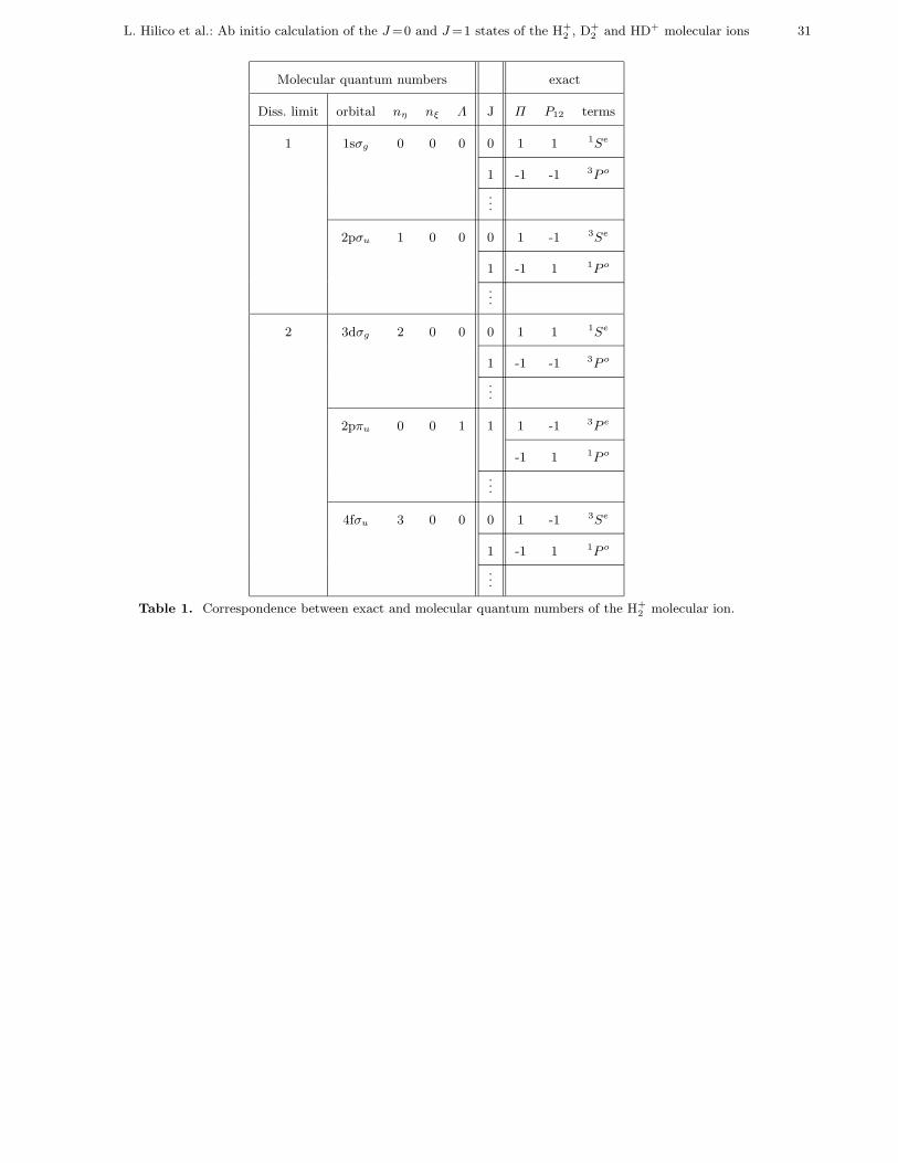
Table 1 gives the correspondence between the exact quantum numbers (for J ≤ 1) and the molecular quantum
numbers, for the electronic states correlated to the two lowest dissociation limits, which support bound vibrational
levels.
3 Numerical Implementation
The Schrodinger equations we have obtained in Sect. 2 have to be solved numerically. The method consists in diag-
onalizing the matrix representing the Hamiltonian in a convenient basis. The choice of the basis has to obey several
constraints if we want to obtain highly accurate well converged energy levels:
– The matrix elements have to be computed using exact simple formulae in closed form.
– For maximum simplicity, we require to use “independent” coordinates, i.e., coordinates in which the Hilbert space
appears as a tensor product of Hilbert spaces along each coordinate. This makes it possible to use basis states
which are tensor products of simple states along each coordinate.
L. Hilico et al.: Ab initio calculation of the J =0 and J =1 states of the H+
2 , D+
2 and HD+ molecular ions 11
– We have to choose a basis in which the Hamiltonian has strong coupling rules – i.e. most of the matrix elements
vanish – to get a sparse band matrix, in order to use very efficient diagonalization algorithms. A sufficient condition
(see below) is that the Hamiltonian can be expressed as a combination of polynomial functions of the coordinates
and the conjugate momenta.
– The long range behavior of the basis functions must be an exponential decrease in the inter-particle distances, as
expected for highly excited states of the three body Coulomb problem.
We now show how those four characteristics can be obtained thanks to the use of the perimetric coordinates.
3.1 Perimetric coordinates
In the Hamiltonian, the potential diverges if one of the inter-particle distances r1, r2 or R vanishes. This divergence
can be regularized through multiplication of the Schrodinger equation by 8r1r2R. Of course, there is a price to pay:
even for S and P e states, the scalar energy E is turned into a positive non diagonal operator E B. The Schrodinger
equation becomes a generalized eigenvalue problem, which is written as:
A|Ψ〉 = E B |Ψ〉, (21)
where A = AS = 8r1r2RHS and B = BS = 8 r1r2R in the case of S states. For P states, the Schrodinger equation
is multiplied by 4 for convenience, so that A = APe
= 32 r1r2R HP e
and B = BPe
= 32 r1r2R3ρ2 for P e states and
A = APo
= 32 r1r2R HP o
and B = BPo
= 32 r1r2R M†M for P o states.
The kinetic terms in the A and B operators are polynomials in R, ρ, ζ, ∂∂R ,
∂∂ρ ,
∂∂ζ , but the potential energy term
in A contains square roots, and we have not been able to find a convenient basis where A has strong coupling
rules. We thus have to use an other set of coordinates. To remove the square roots, we could work with the radial
coordinates (r1, r2, R). The operators A and B are polynomials in r1, r2, R,∂∂r1
, ∂∂r2
, ∂∂R . However, those coordinates
are not independent, since their ranges are connected by the triangular inequalities |r1 − r2| ≤ R ≤ r1 + r2, and
the Hilbert space is not a tensor product of Hilbert spaces along the r1, r2 and R coordinates. The set of spheroıdal
coordinates, inherited from the Born Oppenheimer approximation, is a good candidate to represent the first energy
levels of a given symmetry, as it directly incorporates some useful physical properties of the system. On the other
hand, it lacks any simplicity in the matrix elements, and becomes inappropriate for the heavy numerical calculations
required for highly excited states.
The perimetric coordinates satisfy all the required criteria. They are defined by:
12 L. Hilico et al.: Ab initio calculation of the J =0 and J =1 states of the H+
2 , D+
2 and HD+ molecular ions
x = r1 + r2 −R,
y = r1 − r2 +R,
z = −r1 + r2 +R.
(22)
The ranges of x, y and z are independent. They are 0 ≤ x < ∞, 0 ≤ y < ∞ and 0 ≤ z < ∞. The effect of the parity
and exchange operators on the perimetric coordinates are:
Π : x→ x P12 : x→ x
y → y y → z
z → z z → y,
(23)
They are connected to R, ρ and ζ by:
R =y + z
2,
ρ2 = xyzx+ y + z
(y + z)2, (24)
ζ =(y − z)(2x+ y + z)
4 (y + z).
The expressions of the operators A and B in perimetric coordinates for the S, P e or P o states can be deduced from
the operators in (R, ρ, ζ) by a tedious but straightforward calculation. They are polynomials in x, y, z , ∂∂x , ∂
∂y ,∂∂z .
For example, the operators for S states of H+2 have been published by Saavedra & al [18]. In the Appendix, we give the
integral expressions of the scalar product of two wave functions of a given symmetry, as well as compact expressions
of the S and P e Hamiltonians.
3.2 Choice of the basis
The structure of the partial differential equations we have to solve is now very simple. Each term of the potential or
of the energy operator B is a polynomial in the perimetric coordinates. Each contribution to the kinetic terms is the
product of a polynomial in x, y and z by a first or second order partial derivative with respect to x, y or z. The long
range behavior of the basis functions has to match that of the wave-functions (an exponential decrease in the case of
the Coulomb interaction) in order to obtain a good description of the excited levels with a basis as small as possible.
Therefore, we have to use a basis built with orthonormal functions in each coordinate x, y and z defined in [0,∞[, and
having an exponential decrease at infinity. A solution is to use Laguerre polynomials.
More precisely, a vector of the basis is defined by:
|n(α)x , n(β)
y , n(β)z 〉 = |n(α)
x 〉 ⊗ |n(β)y 〉 ⊗ |n(β)
z 〉, (25)
L. Hilico et al.: Ab initio calculation of the J =0 and J =1 states of the H+
2 , D+
2 and HD+ molecular ions 13
where |n(α)〉 is the basis state whose wave-function is 〈u|n(α)〉 = χ(α)n (u). α and β are two positive real parameters,
whose choice is discussed below. The χ(α)n (u) functions are chosen to be orthonormal with respect to the scalar product
in perimetric coordinates, which depends on the class of states under study (see Appendix A.1). For the S and P o
states, the scalar product in perimetric coordinates involves the weight dx dy dz. Thus we introduce:
χ(α)n (u) = (−1)n
√α L(0)
n (αu) e−αu/2, (26)
where L(p)n are the generalized Laguerre polynomials [19]. These states form a complete orthogonal basis for this scalar
product.
For the P e states, the scalar product involves the weight xdx ydy zdz and we define:
χ(α)n (u) =
(−1)n√α√
n+ 1L(1)n (αu) e−αu/2. (27)
In equation (25), α−1 and β−1 are two length scales. The long range behavior of the basis functions is, in terms of
the radial distances:
e−αr1/2e−αr2/2e(−β+α/2)R. (28)
For homonuclear molecular ions, r1 and r2 play symmetric roles, and it is thus natural to choose the same parameter
β along the y and z coordinates. For most of the energy levels computed here, the optimum values of α and β verify
β >> α, and we can consider that α−1 gives the electronic length scale while β−1 mainly determines the inter-nuclear
length scale. This is no longer true for weakly bound levels, close to a dissociation limit, for which we have α ≈ β.
Because of their structure, all the terms in the Hamiltonian have strong coupling rules (see Appendix A.2): non-zero
matrix elements between |nx, ny, nz〉 and |nx +∆nx, ny +∆ny, nz +∆nz〉 are obtained only if |∆nx|,|∆ny |,|∆nz| and
|∆nx| + |∆ny| + |∆nz| are smaller than 2, 2, 2, 3 for S states, 3, 3, 3, 4 for P e states, and 4, 4, 3, 5 for P o states,
giving respectively 57, 123 and 215 coupling rules. The analytical calculation of the matrix elements of the various
contributions to the Hamiltonian is very tedious and has been performed using the symbolic calculation language Maple
V. The results are directly output in FORTRAN code. An example of such a matrix element is given in Appendix A.2.
For the S and P e states of H+2 and D+
2 , the singlet and triplet wave functions obey the same Schrodinger equation,
the only difference being the symmetric or antisymmetric character with respect to the exchange of y and z. We thus
use a symmetrized or antisymmetrized basis (the length scales α and β are omitted):
|nx, ny, nz〉± =|nx, ny, nz〉 ± |nx, nz, ny〉√
2. (29)
The vector indices are restricted to ny ≤ nz or ny < nz. This symmetrization requires the length scales in the y and
z directions to be equal, in order to preserve the coupling rules.
14 L. Hilico et al.: Ab initio calculation of the J =0 and J =1 states of the H+
2 , D+
2 and HD+ molecular ions
For P o states, the radial F function has no longer any symmetry with respect to the exchange of y and z, so the
basis vectors are simply |nx, ny, nz〉. In the case of S states of HD+, the basis vectors are also |nx, ny, nz〉.
3.3 Numerical diagonalization
To perform the numerical calculations, the basis is truncated at nx + ny + nz ≤ N and nx ≤ Nx, with Nx ≤ N . If
the basis is symmetrized (resp. antisymmetrized), we add the condition ny ≤ nz (resp. ny < nz). The total number of
basis states Ntot scales as N2Nx.
The various basis vectors are ordered using an algorithm which builds a sparse band matrix with a width as small
as possible. The width (defined as the maximum distance in the ordered basis between two coupled vectors) scales as
NNx and it is typically a few percent of the size of the basis. Of course, it increases with the number of coupling rules.
The diagonalization of the generalized eigenvalue problem (21) is performed with the Lanczos algorithm [20]. The
amount of required memory and the efficiency of this algorithm depend on the width of the matrix.
The truncation of the basis turns the length scales α−1 and β−1 into variational parameters. They have to be
optimized, in order to minimize the eigenenergies of the Hamiltonian. Since the dependence on the variational param-
eters decreases if the size of the basis increases, and because we wish to determine as many levels as possible, we have
basis sets as large as possible, limited by the amount of memory of the computers (up to 1 GB is used on our local
workstations, and up to 32 GB on a Cray T3E supercomputer). Both α and β parameters are scanned on a range
large enough to observe the minimum of each eigenvalue. In practice, we obtain, for most of the eigenenergies, a well
defined region in the parameter space, where the energy does not depend on the variational parameters. Then, each
eigenenergy is determined with an accuracy limited only by the numerical noise due to round off errors. A typical
accuracy of the order of 10−14 is reached, as expected in double precision FORTRAN code. The convergence properties
are illustrated in Fig. 2 and Fig. 3. Note that the 10−14 accuracy is obtained for J = 0 states only. For J = 1 states,
there is a small numerical unstability of the algorithm – probably related to the condition number of the matrices A
and B – that prevented us from calculating more than eleven or twelve significant digits.
4 Numerical results
The energies of all the J = 0 and J = 1 bound levels of the H+2 or D+
2 molecular ions below the first dissociation
limit have been computed. As shown in Table 1, the rovibrational levels of the 1sσg electronic ground state have 1Se
or 3P o symmetries, while the 2pσu excited states are either 3Se or 1P o states. There is no P e state below the first
L. Hilico et al.: Ab initio calculation of the J =0 and J =1 states of the H+
2 , D+
2 and HD+ molecular ions 15
dissociation limit (see Table 1). The numerical results we have obtained in that case will be presented elsewhere. The
convergence control procedure is detailed only for the 1Se states, but the same procedure has been used for all the
levels reported here. All the numerical values shown in this paper have been checked to be well converged at the level
of the last printed digit.
The 1986 fundamental constants [21] are used. The proton to electron mass ratio and the deuteron to electron
mass ratio are 1836.152701 and 3670.483014. The atomic unit of energy is 219474.63067 cm−1.
4.1 1Se states of H+2
4.1.1 Convergence region
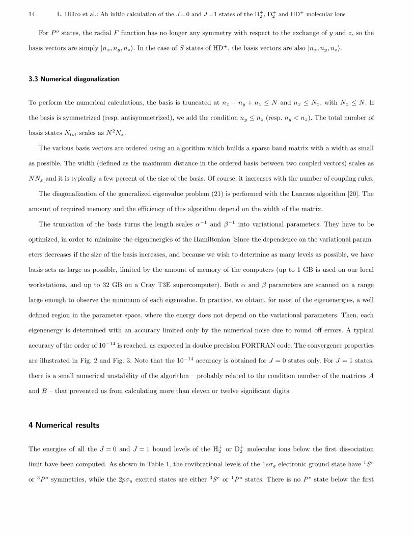
The convergence of the results is illustrated in Figs. 2 to 4. For these computations, the truncation bounds have been
limited to N = 96 and Nx = 20. The basis contains 40846 functions, the (half-)width of the matrix is 1846 and the
required memory is about 500 MBytes. Fig. 2 shows the convergence region in the the (α, β) space for (a) the 5th and
(b) the 18th level. This is a logarithmic contour plot of the difference between the energy obtained for parameters α
and β and the best value obtained with a larger basis (see Table 2). The contour levels are shown in the figure. For
the 5th level, one observes a wide region in which the convergence at the 10−13 level is achieved. The dashed lines
correspond to the 10−14 contour. Its irregular shape arises from the numerical noise. For the 18th level, the energy is
converged only at the 10−13 level in a small region because the basis is not large enough. Of course, convergence at the
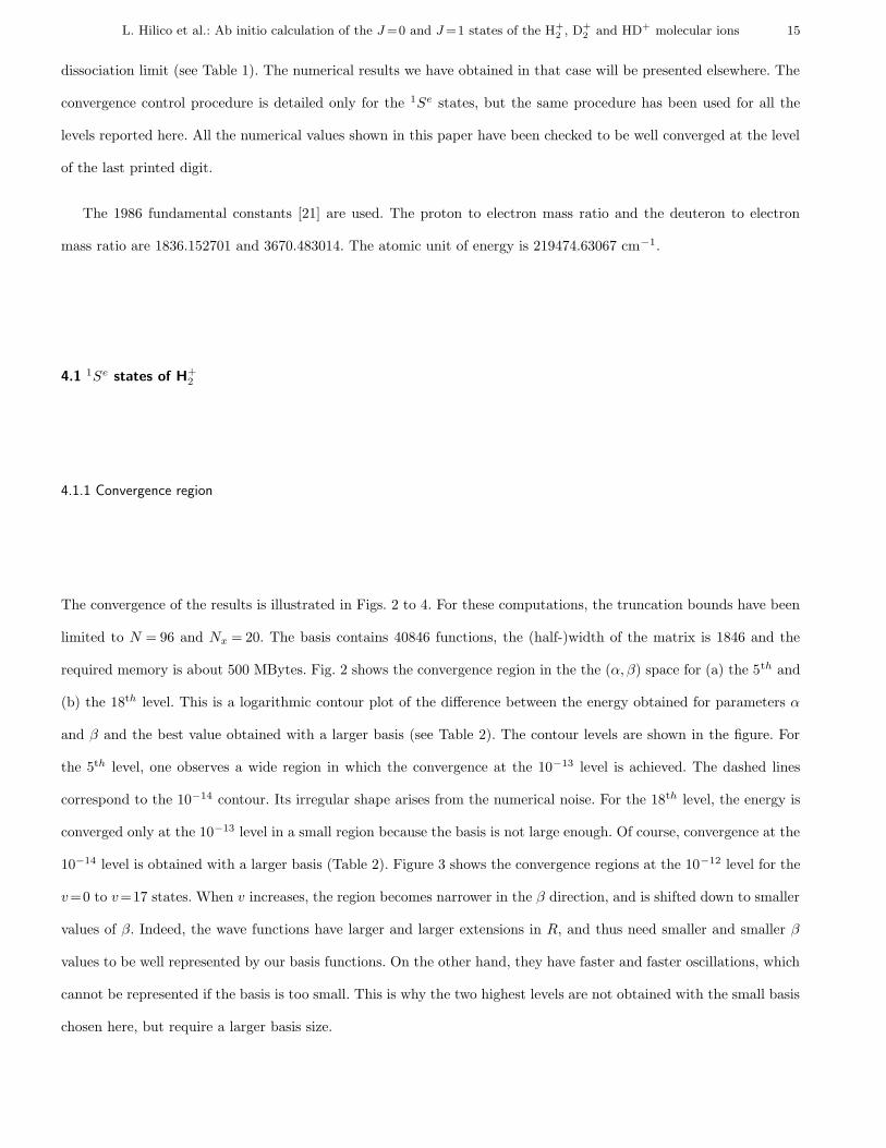
10−14 level is obtained with a larger basis (Table 2). Figure 3 shows the convergence regions at the 10−12 level for the
v=0 to v=17 states. When v increases, the region becomes narrower in the β direction, and is shifted down to smaller
values of β. Indeed, the wave functions have larger and larger extensions in R, and thus need smaller and smaller β
values to be well represented by our basis functions. On the other hand, they have faster and faster oscillations, which
cannot be represented if the basis is too small. This is why the two highest levels are not obtained with the small basis
chosen here, but require a larger basis size.
16 L. Hilico et al.: Ab initio calculation of the J =0 and J =1 states of the H+
2 , D+
2 and HD+ molecular ions
4.1.2 Convergence of the eigenvectors
When the best parameter region is found (around α=1.7 and β=8 from Fig. 3), the quality of the results is checked
by analyzing the eigenvector expansion on the basis. Each eigenvector |Ψ〉 is numerically known as:
|Ψ〉 =∑
0 ≤ nx ≤ Nx
0 ≤ ny ≤ nz ≤ N
nx + ny + nz ≤ N
Cnxnynz|nx, ny, nz〉±. (30)
The eigenvectors |Ψ〉 are normalized for the scalar product defined in Appendix A.1. They verify the normalization
condition 〈Ψ | BS |Ψ〉/32 = 1. We introduce the projection operator Pnxonto the subspace with fixed nx value. We
have:
Pnx|Ψ〉 =
∑
0 ≤ ny ≤ nz ≤ N
ny + nz ≤ N − nx
Cnxnynz|nx, ny, nz〉±. (31)
We then determine the weight of Pnx|Ψ〉 in |Ψ〉 by computing the overlap:
Px(nx) = 〈Ψ | BS Pnx|Ψ〉/32. (32)
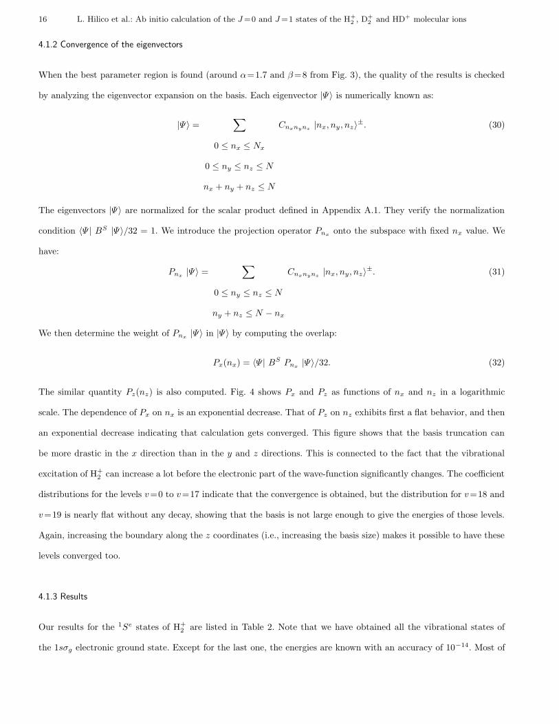
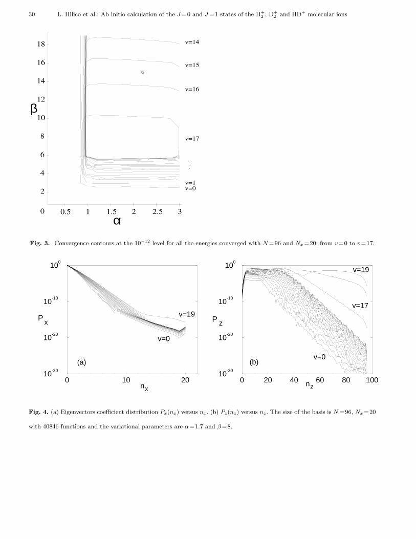
The similar quantity Pz(nz) is also computed. Fig. 4 shows Px and Pz as functions of nx and nz in a logarithmic
scale. The dependence of Px on nx is an exponential decrease. That of Pz on nz exhibits first a flat behavior, and then
an exponential decrease indicating that calculation gets converged. This figure shows that the basis truncation can
be more drastic in the x direction than in the y and z directions. This is connected to the fact that the vibrational
excitation of H+2 can increase a lot before the electronic part of the wave-function significantly changes. The coefficient
distributions for the levels v=0 to v=17 indicate that the convergence is obtained, but the distribution for v=18 and
v=19 is nearly flat without any decay, showing that the basis is not large enough to give the energies of those levels.
Again, increasing the boundary along the z coordinates (i.e., increasing the basis size) makes it possible to have these
levels converged too.
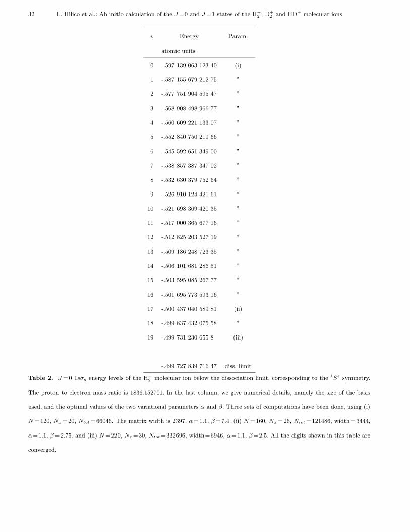
4.1.3 Results
Our results for the 1Se states of H+2 are listed in Table 2. Note that we have obtained all the vibrational states of
the 1sσg electronic ground state. Except for the last one, the energies are known with an accuracy of 10−14. Most of
L. Hilico et al.: Ab initio calculation of the J =0 and J =1 states of the H+
2 , D+
2 and HD+ molecular ions 17
them can be obtained using the truncation bounds N = 120 and Nx = 20. The last vibrational level requires a very
large basis, with N=220 and Nx=30, containing 332696 functions. The values of the variational parameters α and β
for which the results can be obtained are given in the tables. They were chosen close to the center of the convergence
region. The size of the region is shown in Figs. 2 and 3.
4.1.4 Comparison with previously published results
Several authors have published accurate energy levels of some J = 0 1sσg states of H+2 corresponding to the 1Se
symmetry. But, up to now, only R.E. Moss has computed all of them. He achieved fully non adiabatic calculations
using a basis built from Laguerre and Legendre polynomials of the spheroıdal electronic coordinates, and gave all the
dissociation energies with an accuracy of 10−11 [22]. Our results are in full agreement with those of Moss, but with an
improved accuracy.
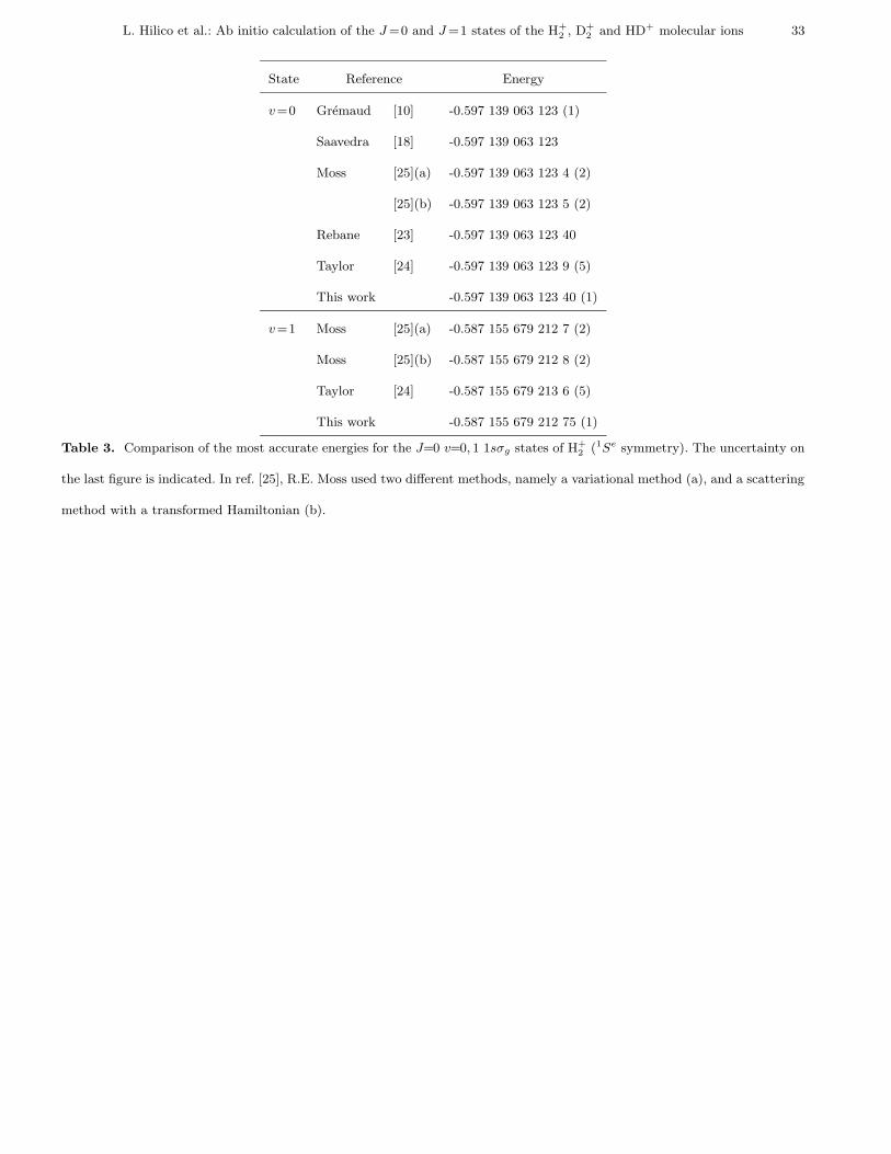
Much more work have been devoted to the two first 1Se states of H+2 , allowing a more detailed comparison, as
summarized in Table 3. In 1998, we have demonstrated the efficiency of our method [10], and given the first two
vibrational levels of H+2 with a 10−12 relative accuracy. At that time, we used only one variational parameter α, and
β had to be set to 2α. Saavedra et al. [18] have published the ground state energy of several three body Coulomb
systems, obtained with exactly the same method. They reached the same accuracy than in [10], but with a much
smaller basis, thanks to the introduction of the second variational parameter β.
T.K. Rebane and A. V. Filinsky [23] have also computed the ground state energy of many three body molecular
ions using perimetric coordinates and variational computations, i.e. a method probably very close to our method, but
still unpublished. The ground state energy of H+2 that they obtained coincides with our values at the 10−14 level.
More recently, two high precision calculations of the energy levels of H+2 have been published [24,25]. Both used a
variational method, which differs from the one described here by the fact that the electronic wave function is expressed
in terms of the prolate spheroıdal coordinates ξ and η. J. M. Taylor et al. [24] have published the first rovibrational
energies of H+2 for (v, J)=(0, 0), (0, 1) and (1, 0) with an accuracy of 5 10−13. R. E. Moss [25] gives the same results,
with a improved accuracy of 10−13. Finally, in the same paper [25], R. E. Moss also uses a scattering method, together
with a transformed Hamiltonian, and obtains results in agreement with the previous ones at the level of 10−13.
In summary, our results are the most accurate ones on the whole sequence of vibrational levels, and agree perfectly
well with the (less accurate) previously published results. This makes us confident on the reliability of our numerical
code.
18 L. Hilico et al.: Ab initio calculation of the J =0 and J =1 states of the H+
2 , D+
2 and HD+ molecular ions
4.2 J=1 1sσg states of H+2
To obtain the rovibrational states of the ground electronic state of H+2 with J = 1, the 3P o Hamiltonian has to be
diagonalized. In that case, the Schrodinger equation is more complicated than in the S state case, since it couples the
radial wave function F (x, y, z) to F (x, y, z) = F (x, z, y) through the exchange terms of the Hamiltonian. The non-zero
matrix elements of the Hamiltonian not only come from the 215 coupling rules of the direct terms, but also from 205
pseudo-rules due to the exchange terms. Indeed, a coupling rule (∆nx, ∆ny, ∆nz) of an exchange term connects the
vector |nx, ny, nz〉 to the vector |n′x, n
′y, n
′z〉 = |nx +∆nx, nz +∆ny, ny +∆nz〉, and induces a pseudo-rule δnx = ∆nx,
δny = n′y − nz and δnz = n′
z − ny. We denote them pseudo-rules because they depend on the values of ny and nz.
Since we have |∆nx| ≤ 4, |∆ny| ≤ 3, |∆nz| ≤ 3 and |∆nx| + |∆ny| + |∆nz| ≤ 5 for the exchange coupling rules,
we obtain 205 pseudo-rules. Finally, we have up to 420 non-zero matrix element per row of the Hamiltonian matrix.
Consequently, the width of the P o matrices is much larger than in the Se case. In addition, for P o states, the basis
is not symmetrized. Thus, for the same bounds on N or Nx, the basis is nearly twice as large. Available computer
memory leads to smaller bounds for P o states than for S states. As a consequence, the accuracy of the eigenenergies
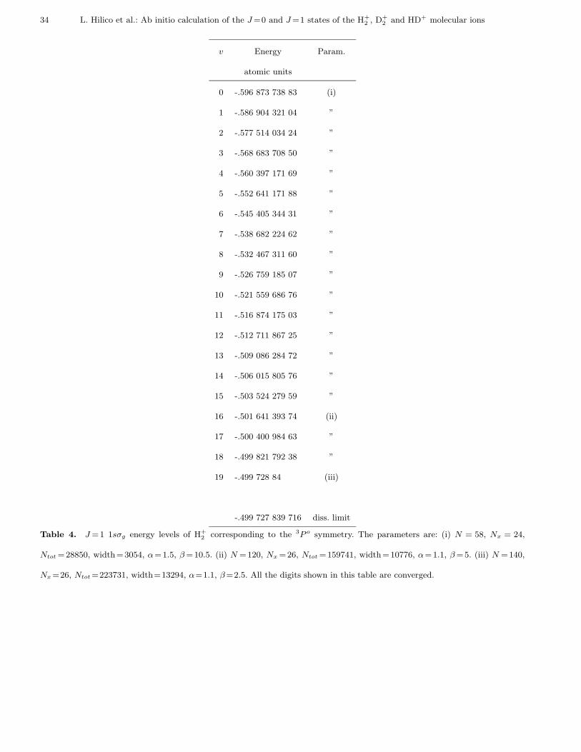
is smaller, and it is difficult to obtain convergence for the highly excited vibrational levels. The energies are given in
Table 4. The accuracy is only at the level of 10−11. This is due to round off errors. Because of the increased sizes of
the matrices, they accumulate more rapidly than for 1Se states; this could also be due to ill-conditioned matrices in
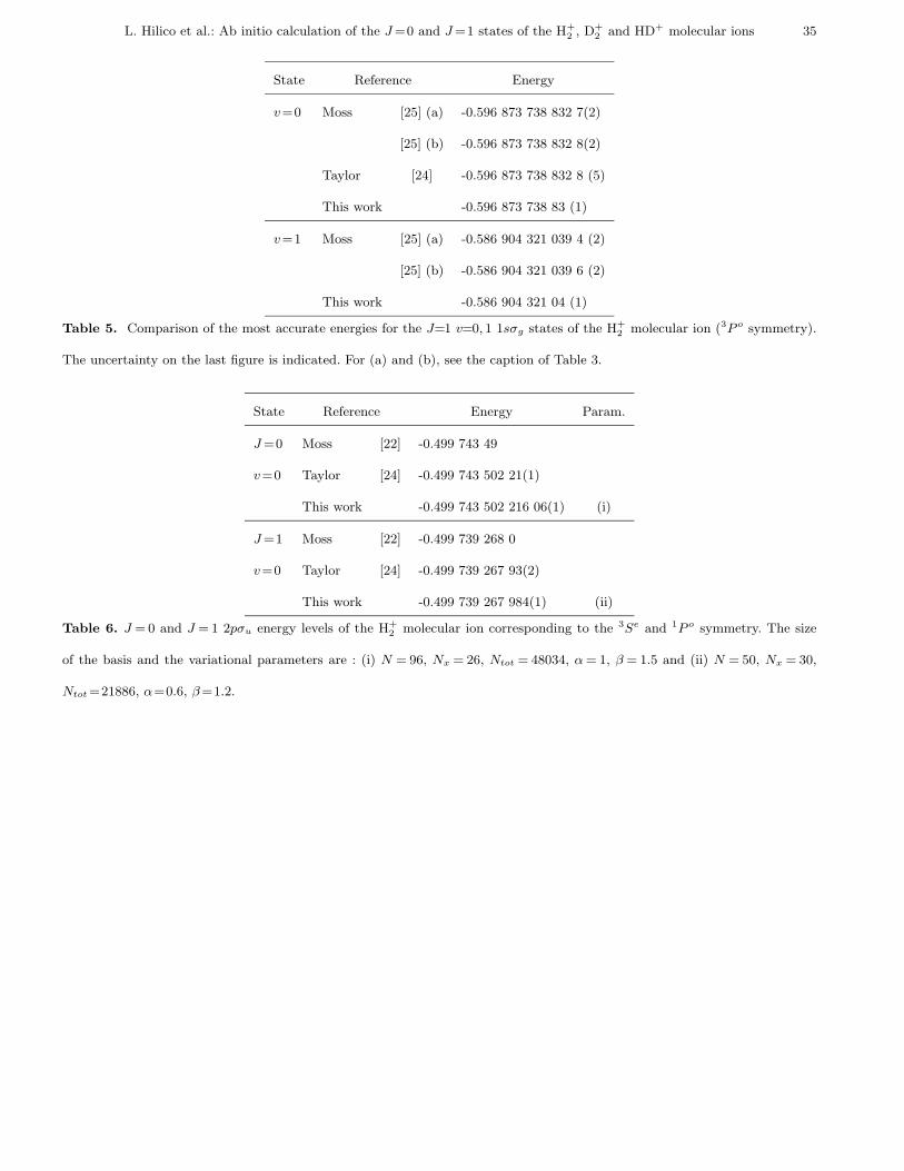
the case of 3P o states, which have eigenvalues separated by several orders of magnitude. In Table 5, we compare our
values to the high accuracy values previously published. Although they are slightly less accurate because of round off
errors, our results agree with the published ones and cover the full sequence of vibrational levels.
4.3 J=0 and J=1 2pσu states of H+2
The 2pσu electronic curve of H+2 has a long range minimum, which supports one bound state for J = 0 or 1. Those
states have either the 3Se or the 1P o symmetries (see Table 1). The computation of the 3Se and 1P o states are similar
to that for the 1Se and 3P o states. The only difference are in Eqs. (18) and (29), where the choice of the + or −
signs has to be inverted. For 3Se states, the indices of the basis vectors have to obey ny < nz . The accuracy for
the 3Se states is better than for the 1P o states, because, for a given amount of memory on the computer, the basis
can be chosen much larger for 3Se states. Since the 1P o state is closer to the dissociation limit, the extension of the
wave function is wider. This explains why the variational parameters are smaller. Table 6 compares our results to the
published values. Again, our values are more accurate, and agree with the previous results.
L. Hilico et al.: Ab initio calculation of the J =0 and J =1 states of the H+
2 , D+
2 and HD+ molecular ions 19
4.4 Results for D+2
Similar calculations have been done for all the Se and P o energy levels of D+2 below the first dissociation limit. We
obtain 28 bound levels corresponding to the 1sσg electronic level of 1Se and 3P o symmetries, listed in Table 7. The
first rovibrational levels are compared with the results already published in Table 8. Finally, Table 9 gives the two
J =0 and the J =1 bound states corresponding to the 2pσu first electronic excited state (3Se and 1P o symmetries),
and compares them with the published values. The conclusions are essentially similar to the ones obtained for H+2 :
with our method, we are able to compute all the vibrational sequence with an improved accuracy. No disagreement is
found with previously published results.
4.5 Mass effect
Highly accurate energy levels of H+2 could be used for measuring the proton to electron mass ratio M/m. A high
accuracy frequency measurement of an optical transition between two rovibrational states of H+2 can be done using a
Doppler free two-photon transition. It should be emphasized that such an experiment will give an information that can
be interpreted either as a M/m measurement, or a study of the relativistic and QED corrections in H+2 . We discuss
here these two aspects.
First, we have determined the dependence of the 1Se energies of H+2 on M/m by computing them for 21 values
of M/m around the 1986 codata values, separated by a 10−5 a.u. step. The slope ∂E∂(M/m) is determined by a least
square linear fit. The results are given in Table 10. The order of magnitude of the slope is a few 10−6 in atomic units.
The third column of Table 10 gives the relative sensitivity of the v → v + 1 transition frequencies on the M/m ratio
defined as:
Tv =M/m
ωv
∂ ωv∂ M/m
, (33)
where ωv denotes the v → v + 1 transition frequency. The order of magnitude of Tv for the first transitions is close to
−0.5, which is the value expected if the nuclear vibration was harmonic. The dependence of Tv on v shows that the
sensitivity of the v → v + 1 transition frequency on M/m decreases with v. M/m is presently known with a relative
accuracy of 2.1 10−9 [26,27]. Thus, the relative uncertainty on the predicted transition frequencies due to the accuracy
of the M/m ratio is of the order of 10−9 for the first transitions. To be compared with some spectroscopic data upon
H+2 , the energies computed here have to be corrected of relativistic and QED effects. Moss [22,28,29] has determined
these relativistic and QED corrections for the rovibrational levels of the 1sσg electronic states. The corrections are
given with an accuracy of 10−4 cm−1. Then, their contribution to the relative uncertainty on the lowest v → v + 1
20 L. Hilico et al.: Ab initio calculation of the J =0 and J =1 states of the H+
2 , D+
2 and HD+ molecular ions
transition frequencies is about 5 10−8. The accuracy of the relativistic and QED corrections has to be improved by at
least two orders of magnitude to allow a M/m measurement through the H+2 spectroscopy. We have briefly discussed
elsewhere the possibility to compute these corrections more accurately [10]. It should be noted that, in any case,
this calculation requires a good knowledge of the exact three body wave functions, which is provided by the method
described in this paper.
In a forthcoming paper, we will present the calculation of the two-photon transition matrix elements between
two rovibrational states of H+2 or D+
2 , and we will discuss the feasibility of a Doppler free two-photon spectroscopy
experiment between two Se states. In such an experiment, the width of the transition is expected to be very small
because the levels are very long lived. Such an experiment could thus measure a transition frequency with a relative
accuracy of 10−10 or better. So far, it would provide a measurement of the difference of the corrections between the two
states involved in the transition, with an accuracy limited by the uncertainty on M/m. Yet any significant progress
on the calculation of the corrections would turn the experiment into a M/m measurement.
5 Se states of HD+
In this section, we give the energies of the 1sσ states of the HD+ molecular ion below the first dissociation limit
(Se symmetry). Here the quantity 1µ12
is computed from the proton to electron mass ratio 1836.152701 and from the
deuteron to proton mass ratio 1.999007496 also taken from [21]. The basis is not symmetrized, and consequently, for
the same truncation bounds as for H+2 , the basis is nearly twice as large. We were able to obtain convergence at the
10−14 level for most of the energy levels on usual workstations, with less than 1 GB of memory. The last vibrationally
excited states required extremely large basis sets, and the last level corresponding to v=22 is converged only at the
10−10 level. The results are given in Table 11. All of them, but the last one, agree with the dissociation energies given
by Moss [30]. Once more, our results are the most accurate ones for the full sequence of vibrational levels.
6 Summary and conclusion
In this paper, we have described a new method to treat a three body Coulomb system. This method takes advantage
of all the symmetries of the system, including dynamical symmetries. Perimetric coordinates are used to describe the
relative positions of the three particles, and generalized Hylleraas type basis functions are introduced, which correctly
describe the asymptotic behavior of the wave-functions. Two length scales are used as variational parameters. Some
comments can be done on this method:
L. Hilico et al.: Ab initio calculation of the J =0 and J =1 states of the H+
2 , D+
2 and HD+ molecular ions 21
a - Obviously, it allows to compute very accurate values of the energy levels of the system. It also provides high
quality wave-functions, as shown by the exponential decrease of the weights in Fig. 4.
b - Because the basis functions have been chosen with the convenient asymptotic behavior, this method is suitable
to accurately describe the highly excited vibrational levels. The electronically excited states can also be described,
if the complex rotation method is used [11,12].
c - Our method is deeply J dependent. We used it here to study the J=0 and J=1 states. Obviously, for higher J
values, this method is less and less convenient. It is suitable only for very low J values.
The method is here applied to the H+2 molecular ion and its isotopomers D+
2 and HD+. The energies of all the
J=0 and 1 states below the first dissociation limit have been computed. Our results are given with a accuracy up to
10−14 atomic unit. Their dependences on the proton to electron mass ratio M/m are also given. Finally, the interest
of a high precision two-photon spectroscopy experiment in H+2 is discussed. Presently, such an experiment would give
information on the relativistic and radiative corrections. Only if the theoretical predictions of those corrections would
be known with two additional figures, a measurement of M/m with some metrological interest could be extracted
from such an experiment.
Laboratoire Kastler Brossel de l’Universite Pierre et Marie Curie et de l’Ecole Normale Superieure is UMR 8552 du
CNRS. We are grateful to IDRIS, which has provided us with many hours of computation on large memory computer
facilities. We are also grateful to Philippe Thomen, who has worked on the derivation of the HD+ Hamiltonian in
perimetric coordinates. The authors thank P. Indelicato for a careful reading of the manuscript.
A APPENDIX
A.1 Scalar product expressions
We recall here the structure of the wave-functions, and give the radial part of the scalar products for the S, P e and
P o states. The angular part of the scalar product is normalized using the standard spherical harmonics. The volume
element is :
R2 dR ρdρ dζ = (x+ y)(x+ z)(y + z)/32 dx dy dz.
In each case, the scalar product involves the positive B operator (representing the energy operator).
For Se states:
Ψ =1√8π2
ϕ(x, y, z),
22 L. Hilico et al.: Ab initio calculation of the J =0 and J =1 states of the H+
2 , D+
2 and HD+ molecular ions
〈Ψ1|Ψ2〉S =
⟨ϕ1
∣∣∣∣BS
32
∣∣∣∣ ϕ2
⟩=
∫ ∫ ∫(x+ y)(y + z)(z + x)
32ϕ∗
1(x, y, z)ϕ2(x, y, z) dx dy dz.
For P e states:
Ψ =(D1∗
M,1(ψ, θ, φ) +D1∗M,−1(ψ, θ, φ))
√2
Rρ ϕ(x, y, z),
〈Ψ1|Ψ2〉Pe
=
⟨ϕ1
∣∣∣∣BP
e
128
∣∣∣∣ ϕ2
⟩
=
∫ ∫ ∫(x+ y + z)(x+ y)(y + z)(z + x)
128ϕ∗
1(x, y, z)ϕ2(x, y, z)xdx ydy zdz.
For P o states:
Ψ = D1∗M,0(ψ, θ, φ) Φ0(x, y, z) +
(D1∗M,−1(ψ, θ, φ) −D1∗
M,1(ψ, θ, φ))√
2Φ1(x, y, z)
with
Φ0
Φ1
= M
F
G
,
〈Ψ1|Ψ2〉Po
=
⟨F1
G1
∣∣∣∣BP
o
128
∣∣∣∣
F2
G2
⟩, (34)
〈Ψ1|Ψ2〉Po
=
∫ ∫ ∫(x+ y)(y + z)(z + x)
128F1
G1
†
(x+ y)2 x(x+ y + z) − yz
x(x+ y + z) − yz (x+ z)2
F2
G2
dx dy dz.
A.2 Derivation of the matrix elements of S and P o states
As mentioned in Sect. 3.2, when using the perimetric coordinates x, y, z, each term of the kinetic part of the Hamil-
tonian appears as a product of a polynomial in x, y, z by a first or second order partial derivative with respect to
x, y and z. In order to obtain the matrix elements of the Hamiltonian, we have to efficiently take into account the
recurrence and differential properties of the Laguerre polynomials family [19]. At a deeper level, we can construct a
Lie algebra of operators that have simple connections with the various operators of interest (i.e., perimetric coordi-
nates and associated momenta) such that the Hilbert space appears as a representation (preferably irreducible) of the
associated Lie group.
L. Hilico et al.: Ab initio calculation of the J =0 and J =1 states of the H+
2 , D+
2 and HD+ molecular ions 23
In the specific case of S and P o states of H+2 or HD+, we introduce the following hermitean operators, written for
a variable u, and a length scale α−1:
S1 =1
α
(u∂2
∂u2+
∂
∂u
)+ α
u
4,
S2 = i
(u∂
∂u+
1
2
), (35)
S3 = − 1
α
(u∂2
∂u2+
∂
∂u
)+ α
u
4.
The commutation relations of those operators are closed:
[S1, S2] = −iS3 , [S2, S3] = iS1 , [S3, S1] = iS2, (36)
and characterize the SO(2, 1) group (Lorentz group in two spatial dimensions). Thus S1, S2 and S3 appear as the
generators of a SO(2, 1) group and Eqs. (35) define a representation of SO(2, 1) for which the Casimir operator can be
computed as S21 + S2
2 − S23 = 1
4 . It follows that the Hilbert space is a single irreducible representation of the SO(2, 1)
group of type D+1/2 [31].
u, u ∂∂u and u ∂2
∂u2 can be expressed as linear combinations of S1, S2 and S3, and consequently, each term of the
Hamiltonian can be expressed as a combination of the generators of three different SO(2, 1) groups.
For the S state Hamiltonian, the expressions are simpler if the following hermitean operators U = S1 + S3,
P = S1 − S3, Q = S21 − S2
3 and S = (S1 + S3) S2 + S2 (S1 + S3) are introduced. For example, we give the expressions
of the operators A and B of Eq. (21):
AS = α−1
(AS1 +
1
2µ12AS2 +
1
2µ0AS3
)+ α−2 V S ,
AS1 = −4 γ2 (Uy + Uz)2 Px − 4 γ (Uy + Uz) Qx
−4 γ(U2z Py + U2
y Pz + Uz Qy + Uy Qz − iSy iS2z − iSz iS2y
),
AS2 = −4 γ2 (U2y + U2
z ) Px − 4 γ (Uy + Uz) Qx
− 8
γ
(U2x +
γ2
2U2z + γUx Uz
)Py − 8 (Ux +
γ
2Uz) Qy
− 8
γ
(U2x +
γ2
2U2y + γUx Uy
)Pz − 8 (Ux +
γ
2Uy) Qz
+4 iSx (iS2y + iS2z) + 4 iS2x (iSy + iSz),
AS3 = 4 γ Qx (Uy − Uz) − 4 iSx (iS2y − iS2z) + 4 γ iS2x (iSz − iSy)
+8 Ux (UyPz − UzPy) + 4 γ2 Px (U2y − U2
z ) + 4 γ (U2y Pz − U2
z Py)
−4 γ (Qy Uz −Qz Uy),
24 L. Hilico et al.: Ab initio calculation of the J =0 and J =1 states of the H+
2 , D+
2 and HD+ molecular ions
V S = −16γ(Ux +
γ
2(Uy + Uz)
)(Uy + Uz) + 8 (Ux + γUy)(Ux + γUz),
BS = 8 α−3 γ (Ux + γUy)(Ux + γUz)(Uy + Uz),
where γ = α/β.
As all the operators involved in the generalized eigenvalue problem, Eq. (21), can be expressed in terms of the
generators S1, S2 and S3, it is natural to use a basis where the generators have simple matrix elements. We choose
the standard basis for the D+1/2 representation of the SO(2, 1) group [31], i.e., eigenstates of the S3 operator that are
labelled with a non-negative integer n. All matrix elements of the generators are known and simple. They have strong
coupling rules (n changes by at most one unit) and are given by:
S1|n > =n+ 1
2|n+ 1 > +
n
2|n− 1 >,
iS2|n > =n+ 1
2|n+ 1 > −n
2|n− 1 >, (37)
S3|n > =
(n+
1
2
)|n > .
The wave-functions in the standard basis are also known. They are:
〈u|n(α)〉 = (−1)n√α L(0)
n (αu) e−αu/2. (38)
A vector of the basis used for the full problem (defined in Eq. (25)) is a tensor product over the three perimetric
coordinates |n(α)x , n
(β)y , n
(β)z 〉, where different length scales are used in the x and y, z coordinates.
From the coupling rule |∆n| ≤ 1 of the elementary operators S1, iS2, S3, one can deduce those of U and P
(|∆n| ≤ 1) and of Q and iS (|∆n| ≤ 2). The detailed expression of the Se Hamiltonian shows that the coupling rules
connecting the basis vectors |nx, ny, nz〉 and |nx + ∆nx, ny + ∆ny, nz + ∆nz〉 are given by |∆nx| ≤ 2, |∆ny| ≤ 2,
|∆nz | ≤ 2 and |∆nx| + |∆ny| + |∆nz | ≤ 3 as announced in Sect. 3.2. The matrix elements of the Hamiltonian can be
easily deduced from those of S1, iS2, S3, using a symbolic calculation language like Maple V. Here, we only give as
an example the diagonal matrix element of the term depending on m/M :
〈a, b, c|AS2 |a, b, c〉 = − (4 + 8 γ b c+ 2 γ + 12 a+ 4 b+ 6 γ3 a b2
+6 γ3 a b+ 6 γ3 a c2 + 6 γ3 a c
+16 γ a b c+ 6 γ b+ 2 γ2 a2 b+ 2 γ2 a b
+2 γ2 a2 c+ 2 γ2 a c+ 2 γ b2 + 4 γ a+ 6 γ c
+2 γ c2 + 6 γ2 b+ 2 γ2 a+ 2 γ2 + 4 γ3 a
+3 γ3 b2 + 2 γ3 + 12 a2 + 12 a b+ 12 a2 b+ 12 a c
L. Hilico et al.: Ab initio calculation of the J =0 and J =1 states of the H+
2 , D+
2 and HD+ molecular ions 25
+4 c+ 12 a2 c+ 4 γ a b2 + 4 γ a c2 + 12 γ a b+ 12 γ a c
+16 γ2 b c+ 4 γ2 b2 + 4 γ2 c2
+6 γ2 c+ 2 γ2 a2 + 3 γ3 c+ 3 γ3 c2
+8 γ2 b2 c+ 8 γ2 b c2 + 3 γ3 b)/γ.
The terms of the operator APo
can be expressed using the same elementary operators. The expressions are too long
to be reported here.
A.3 Derivation of the matrix elements of P e states
In the case of P e states, because the scalar product involves the weight xdx ydy zdz, the previous generators are no
longer hermitean. We thus have to define a new set of hermitean operators:
S1 =1
α
(u∂2
∂u2+ 2
∂
∂u
)+ α
u
4,
S2 = i
(u∂
∂u+ 1
), (39)
S3 = − 1
α
(u∂2
∂u2+ 2
∂
∂u
)+ α
u
4.
The commutation relations are still [S1, S2] = −iS3, [S2, S3] = iS1 and [S3, S1] = iS2, and the interpretation in terms
of group theory is similar. The Casimir operator is now computed as S21 +S2
2 −S23 = 0. Thus, the Hilbert space spans
a D+1 representation of the SO(2, 1) group. The standard basis is again composed of eigenstates of S3 and the matrix
elements of the generators are:
S1|n > =
√(n+ 1)(n+ 2)
2|n+ 1 > +
√n(n+ 1)
2|n− 1 >,
iS2|n > =
√(n+ 1)(n+ 2)
2|n+ 1 > −
√n(n+ 1)
2|n− 1 >,
S3|n > = (n+ 1)|n > .
Finally, the wave-functions of the basis states are:
〈u|n(α)〉 =(−1)n
√α√
n+ 1L(1)n (αu) e−αu/2. (40)
The expression of the P e Hamiltonian involves the hermitean operators U = S1 + S3, M = S1 − S3, Q = S21 − S2
3 ,
N = (S1 + S3) S2 + S2 (S1 + S3), F = U M U and G = U S2 U . We have:
APe
= α−2
(AP
e
1 +1
2µ12AP
e
2 +1
2µ0AP
e
3
)+ α−3 V P
e
, (41)
26 L. Hilico et al.: Ab initio calculation of the J =0 and J =1 states of the H+
2 , D+
2 and HD+ molecular ions
APe
1 = 8 γ3 (−Mx Uy3 − 3Mx Uy
2 Uz − 3Mx Uy Uz2 − Mx Uz
3)
+8 γ2 (−Uy3 Mz − My Uz
3 − 2Qx Uy2 − 4Qx Uy Uz − 2Qx Uz
2 − 2Uy2 Qz
− 2Qy Uz2 − Uy Uz − Uy Fz − Fy Uz + iNy iNz + 2 iS2y iGz + 2 iGy iS2z )
+8 γ (−Ux Uy2 Mz − Ux My Uz
2 − Ux Uy Qz − Ux Qy Uz + Ux iNy iS2z
+ Ux iS2y iNz − Fx Uy − Fx Uz ),
APe
2 = −8 γ3 (Mx Uy3 + Mx Uy
2 Uz + Mx Uy Uz2 + Mx Uz
3)
+8 γ2 (−Uy3 Mz − My Uz
3 − 2Qx Uy2 − 2Qx Uy Uz − 2Qx Uz
2
+ iS2x Uy iNz + iS2x iNy Uz − 2Uy2 Qz − 2Qy Uz
2 + 2 iS2x iGy + 2 iS2x iGz
− Uy Fz − Fy Uz )
+8 γ (−3Ux Uy2 Mz − 3Ux My Uz
2 − 5Ux Uy Qz
− 5Ux Qy Uz + iNx Uy iS2z + iNx iS2y Uz − Ux Uy − 2Ux Fy − Ux Uz
− 2Ux Fz − Fx Uy − Fx Uz + iNx iNy + iNx iNz )
+16 (−2Ux2 Uy Mz − 2Ux
2 My Uz − 2Ux2 Qy − 2Ux
2 Qz + iGx iS2y + iGx iS2z )
+−16Ux
3 My − 16Ux3 Mz
γ,
APe
3 = 16(Ux2 Uy Mz − Ux
2 My Uz − iGx iS2y + iGx iS2z )
+ 8 γ3 (Mx Uy3 + Mx Uy
2 Uz − Mx Uy Uz2 − Mx Uz
3)
+8 γ2 (Uy3 Mz − My Uz
3 + 2Qx Uy2 − 2Qx Uz
2
+ iS2x Uy iNz − iS2x iNy Uz + 2Uy2 Qz − 2Qy Uz
2
− 2 iS2x iGy + 2 iS2x iGz + Uy Fz − Fy Uz )
+8 γ (3Ux Uy2 Mz − 3Ux My Uz
2
+ 3Ux Uy Qz − 3Ux Qy Uz + iNx Uy iS2z − iNx iS2y Uz + Ux Uy − Ux Uz
+ Fx Uy − Fx Uz − iNx iNy + iNx iNz ),
V Pe
= −16 γ (Uz + Uy) (γUy + γ Uz + 2Ux ) (Ux + γ Uy + γ Uz )
+ 16 (γUy + Ux ) (Ux + γ Uz ) (Ux + γ Uy + γ Uz ),
L. Hilico et al.: Ab initio calculation of the J =0 and J =1 states of the H+
2 , D+
2 and HD+ molecular ions 27
BPe
= 16α−4 γ (Uz + Uy) (γUy + Ux ) (Ux + γ Uz ) (Ux + γ Uy + γ Uz ).
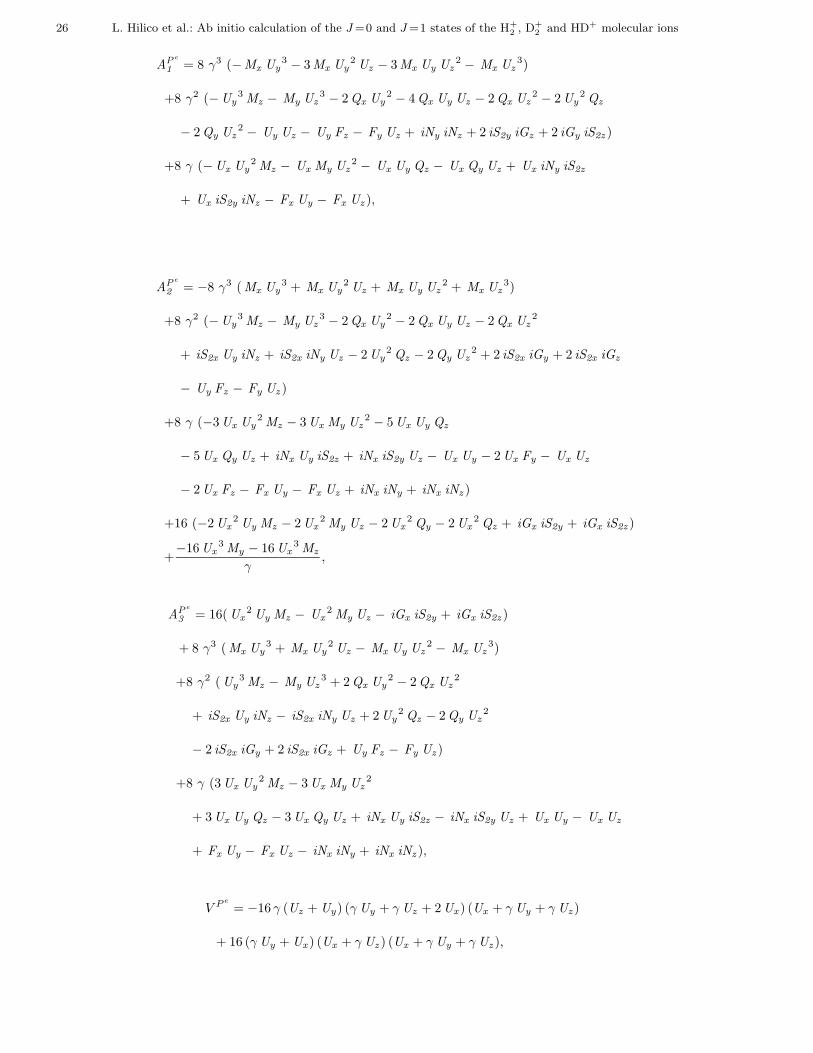
The coupling rules are |∆n| ≤ 1 for U and M , |∆n| ≤ 2 for Q and iN , and |∆n| ≤ 3 for F and iG. The structure
of the Hamiltonian explains the coupling rules |∆nx| ≤ 3, |∆ny| ≤ 3, |∆nz | ≤ 3 and |∆nx| + |∆ny| + |∆nz | ≤ 4 given
in Eq. (3.2).
References
1. Pauli studied H+
2 in the frame of the old quantum theory in his thesis work: W. Pauli, Ann. Phys. (Leipzig) 68, 177 (1922).
2. See for instance: J.C. Slater, Quantum theory of matter, (McGraw Hill, New York, 1968).
3. W. G. Sturrus, E. A. Hessels, P. W. Arcuni, S.R. Lundeen, Phys. Rev. A44, 3032 (1991); P. L. Jacobson, D. S. Fisher, C.
W. Fehrenbach, W. G. Sturrus, S.R. Lundeen, Phys. Rev. A56, R4361, (1997) and Phys. Rev. A57, 4065 (1998).
4. R. E. Moss, Phys. Rev. A. 58, 4447 (1998).
5. J. M. Taylor, A. Dalgarno, J. F. Babb, Phys. Rev. A. 60, R2630 (1999).
6. L. Wolniewicz, J. D. Poll, J. Chem. Phys. 73, 6225 (1980); L. Wolniewicz, J. D. Poll, Molec. Phys. 59, 953 (1986);
L. Wolniewicz, T. Orlikowski, Molec. Phys. 74, 103 (1991).
7. D. M. Bishop, S. A. Solunac, Phys. Rev. Lett. 55, 1986 (1985).
8. R. E. Moss, I. A. Sadler, Molec. Phys. 68, 1015 (1993).
9. G. G. Balint-Kurti, R. E. Moss, I. A. Sadler, M. Shapiro, Phys. Rev A 41, 4913 (1990).
10. B. Gremaud, D. Delande, N. Billy, J. Phys. B 31, 383 (1998).
11. K. Richter, J. S. Briggs, D. Wintgen, E. A. Solov’ev, J. Phys. B 25, 3929 (1992).
12. B. Gremaud, Ph. D. Thesis, University Pierre et Marie Curie (Paris 6), (1997).
13. A. Messiah, Mecanique Quantique-tome 2, (Dunod, Paris, 1964).
14. D. Wintgen, D. Delande, J. Phys. B 26, L399 (1993).
15. M. Pont, R. Shakeshaft, Phys. Rev. A 51, 257 (1995).
16. P. M. Morse, H. Feshbach, Methods of theoretical physics, Chap. 12, (McGraw Hill, New York, 1953).
17. B. R. Judd, Angular Momentum Theory for Diatomic Molecules, (Academic Press, New York, 1975).
18. F. Arias de Saavedra, E. Buendıa, F. J. Galvez, A. Sarsa, Eur. Phys. J. D 2, 181 (1998).
19. M. Abramovitz, I.A. Stegun, Handbook of mathematical functions, (Dover, New York, 1972).
20. T. Ericsson, A. Ruhe, Math. Comput. 35, 1251 (1980), and references therein.
21. E. R. Cohen, B. N. Taylor, Rev. Mod. phys., 59, 1121 (1987).
22. R. E. Moss, Molec. Phys. 80, 1541 (1993).
23. T. K. Rebane, A. V. Filinsky, Physics of Atomic Nuclei 60, 1816 (1997).

28 L. Hilico et al.: Ab initio calculation of the J =0 and J =1 states of the H+
2 , D+
2 and HD+ molecular ions
24. J. M. Taylor, Zong-Chao Yan, A. Dalgarno, J. F. Babb, Molec. Phys. 97, 1 (1999).
25. R. E. Moss, J. Phys. B, 32, L89 (1999).
26. D. L. Farnham, R. S. Van Dick, P. B. Schwinberg, Phys. Rev. Lett. 75, 3598 (1995).
27. P.J. Mohr, B.N. Taylor, Journ. of phys. and chem. reference data, 28, 1713 (1999).
28. M. H. Howells, R. A. Kennedy, J. Chem. Soc. Faraday Trans., 86, 3495 (1990).
29. R. Bukowski, B. Jeziorski, R. Mozynski, W. Kolos, Int. J. Quant. Chem., 42, 287 (1992).
30. R. E. Moss, Molec. Phys. 78, 371 (1993).
31. A.O. Barut and R. Raczka, Theory of Group Representations and Applications, PWN (Warsaw, 1980); D. Delande, These
d’Etat, in french, Universite Pierre et Marie Curie (Paris, 1988).
L. Hilico et al.: Ab initio calculation of the J =0 and J =1 states of the H+
2 , D+
2 and HD+ molecular ions 29
0.0 10.0 20.0 30.0Internuclear distance R (a.u.)
-0.7
-0.6
-0.5
-0.4
-0.3
-0.2
-0.1
0.0en
ergy
(a.
u.)
1,0,0
2,0,0
3,0,0
0,0,1
0,0,0
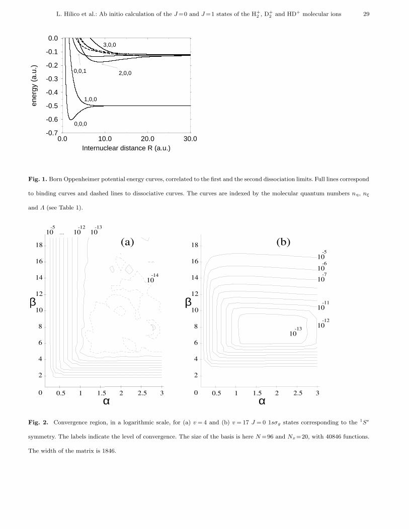
Fig. 1. Born Oppenheimer potential energy curves, correlated to the first and the second dissociation limits. Full lines correspond
to binding curves and dashed lines to dissociative curves. The curves are indexed by the molecular quantum numbers nη, nξ
and Λ (see Table 1).
α32.521.510.5
β
18
16
14
12
10
8
6
4
2
0
101010
10
-13-12-5...
-14
(a)
α32.521.510.5
β
18
16
14
12
10
8
6
4
2
0
10
1010
10
1010
-5
-6
-7
-11
-12-13
(b)
Fig. 2. Convergence region, in a logarithmic scale, for (a) v = 4 and (b) v = 17 J = 0 1sσg states corresponding to the 1Se
symmetry. The labels indicate the level of convergence. The size of the basis is here N =96 and Nx =20, with 40846 functions.
The width of the matrix is 1846.
30 L. Hilico et al.: Ab initio calculation of the J =0 and J =1 states of the H+
2 , D+
2 and HD+ molecular ions
α32.521.510.5
β
18
16
14
12
10
8
6
4
2
0
v=17
v=16
v=15
v=14
v=0v=1
..
.
Fig. 3. Convergence contours at the 10−12 level for all the energies converged with N =96 and Nx =20, from v=0 to v=17.
0 10 2010
-30
10-20
10-10
100
n
v=0
x
(a)
v=19P x
0 20 40 60 80 10010
-30
10-20
10-10
100
v=0
v=17
v=19
(b)
nz
P z
Fig. 4. (a) Eigenvectors coefficient distribution Px(nx) versus nx. (b) Pz(nz) versus nz. The size of the basis is N =96, Nx =20
with 40846 functions and the variational parameters are α=1.7 and β=8.
L. Hilico et al.: Ab initio calculation of the J =0 and J =1 states of the H+
2 , D+
2 and HD+ molecular ions 31
Molecular quantum numbers exact
Diss. limit orbital nη nξ Λ J Π P12 terms
1 1sσg 0 0 0 0 1 1 1Se
1 -1 -1 3P o
...
2pσu 1 0 0 0 1 -1 3Se
1 -1 1 1P o
...
2 3dσg 2 0 0 0 1 1 1Se
1 -1 -1 3P o
...
2pπu 0 0 1 1 1 -1 3P e
-1 1 1P o
...
4fσu 3 0 0 0 1 -1 3Se
1 -1 1 1P o
...
Table 1. Correspondence between exact and molecular quantum numbers of the H+
2 molecular ion.
32 L. Hilico et al.: Ab initio calculation of the J =0 and J =1 states of the H+
2 , D+
2 and HD+ molecular ions
v Energy Param.
atomic units
0 -.597 139 063 123 40 (i)
1 -.587 155 679 212 75 ”
2 -.577 751 904 595 47 ”
3 -.568 908 498 966 77 ”
4 -.560 609 221 133 07 ”
5 -.552 840 750 219 66 ”
6 -.545 592 651 349 00 ”
7 -.538 857 387 347 02 ”
8 -.532 630 379 752 64 ”
9 -.526 910 124 421 61 ”
10 -.521 698 369 420 35 ”
11 -.517 000 365 677 16 ”
12 -.512 825 203 527 19 ”
13 -.509 186 248 723 35 ”
14 -.506 101 681 286 51 ”
15 -.503 595 085 267 77 ”
16 -.501 695 773 593 16 ”
17 -.500 437 040 589 81 (ii)
18 -.499 837 432 075 58 ”
19 -.499 731 230 655 8 (iii)
-.499 727 839 716 47 diss. limit
Table 2. J =0 1sσg energy levels of the H+
2 molecular ion below the dissociation limit, corresponding to the 1Se symmetry.
The proton to electron mass ratio is 1836.152701. In the last column, we give numerical details, namely the size of the basis
used, and the optimal values of the two variational parameters α and β. Three sets of computations have been done, using (i)
N =120, Nx =20, Ntot =66046. The matrix width is 2397. α=1.1, β =7.4. (ii) N =160, Nx =26, Ntot =121486, width=3444,
α=1.1, β =2.75. and (iii) N =220, Nx =30, Ntot =332696, width=6946, α=1.1, β =2.5. All the digits shown in this table are
converged.
L. Hilico et al.: Ab initio calculation of the J =0 and J =1 states of the H+
2 , D+
2 and HD+ molecular ions 33
State Reference Energy
v=0 Gremaud [10] -0.597 139 063 123 (1)
Saavedra [18] -0.597 139 063 123
Moss [25](a) -0.597 139 063 123 4 (2)
[25](b) -0.597 139 063 123 5 (2)
Rebane [23] -0.597 139 063 123 40
Taylor [24] -0.597 139 063 123 9 (5)
This work -0.597 139 063 123 40 (1)
v=1 Moss [25](a) -0.587 155 679 212 7 (2)
Moss [25](b) -0.587 155 679 212 8 (2)
Taylor [24] -0.587 155 679 213 6 (5)
This work -0.587 155 679 212 75 (1)
Table 3. Comparison of the most accurate energies for the J=0 v=0, 1 1sσg states of H+
2 (1Se symmetry). The uncertainty on
the last figure is indicated. In ref. [25], R.E. Moss used two different methods, namely a variational method (a), and a scattering
method with a transformed Hamiltonian (b).
34 L. Hilico et al.: Ab initio calculation of the J =0 and J =1 states of the H+
2 , D+
2 and HD+ molecular ions
v Energy Param.
atomic units
0 -.596 873 738 83 (i)
1 -.586 904 321 04 ”
2 -.577 514 034 24 ”
3 -.568 683 708 50 ”
4 -.560 397 171 69 ”
5 -.552 641 171 88 ”
6 -.545 405 344 31 ”
7 -.538 682 224 62 ”
8 -.532 467 311 60 ”
9 -.526 759 185 07 ”
10 -.521 559 686 76 ”
11 -.516 874 175 03 ”
12 -.512 711 867 25 ”
13 -.509 086 284 72 ”
14 -.506 015 805 76 ”
15 -.503 524 279 59 ”
16 -.501 641 393 74 (ii)
17 -.500 400 984 63 ”
18 -.499 821 792 38 ”
19 -.499 728 84 (iii)
-.499 727 839 716 diss. limit
Table 4. J =1 1sσg energy levels of H+
2 corresponding to the 3P o symmetry. The parameters are: (i) N = 58, Nx = 24,
Ntot =28850, width=3054, α=1.5, β =10.5. (ii) N =120, Nx =26, Ntot =159741, width=10776, α=1.1, β =5. (iii) N =140,
Nx =26, Ntot =223731, width=13294, α=1.1, β=2.5. All the digits shown in this table are converged.
L. Hilico et al.: Ab initio calculation of the J =0 and J =1 states of the H+
2 , D+
2 and HD+ molecular ions 35
State Reference Energy
v=0 Moss [25] (a) -0.596 873 738 832 7(2)
[25] (b) -0.596 873 738 832 8(2)
Taylor [24] -0.596 873 738 832 8 (5)
This work -0.596 873 738 83 (1)
v=1 Moss [25] (a) -0.586 904 321 039 4 (2)
[25] (b) -0.586 904 321 039 6 (2)
This work -0.586 904 321 04 (1)
Table 5. Comparison of the most accurate energies for the J=1 v=0, 1 1sσg states of the H+
2 molecular ion (3P o symmetry).
The uncertainty on the last figure is indicated. For (a) and (b), see the caption of Table 3.
State Reference Energy Param.
J =0 Moss [22] -0.499 743 49
v=0 Taylor [24] -0.499 743 502 21(1)
This work -0.499 743 502 216 06(1) (i)
J =1 Moss [22] -0.499 739 268 0
v=0 Taylor [24] -0.499 739 267 93(2)
This work -0.499 739 267 984(1) (ii)
Table 6. J = 0 and J = 1 2pσu energy levels of the H+
2 molecular ion corresponding to the 3Se and 1P o symmetry. The size
of the basis and the variational parameters are : (i) N = 96, Nx = 26, Ntot = 48034, α = 1, β = 1.5 and (ii) N = 50, Nx = 30,
Ntot =21886, α=0.6, β=1.2.
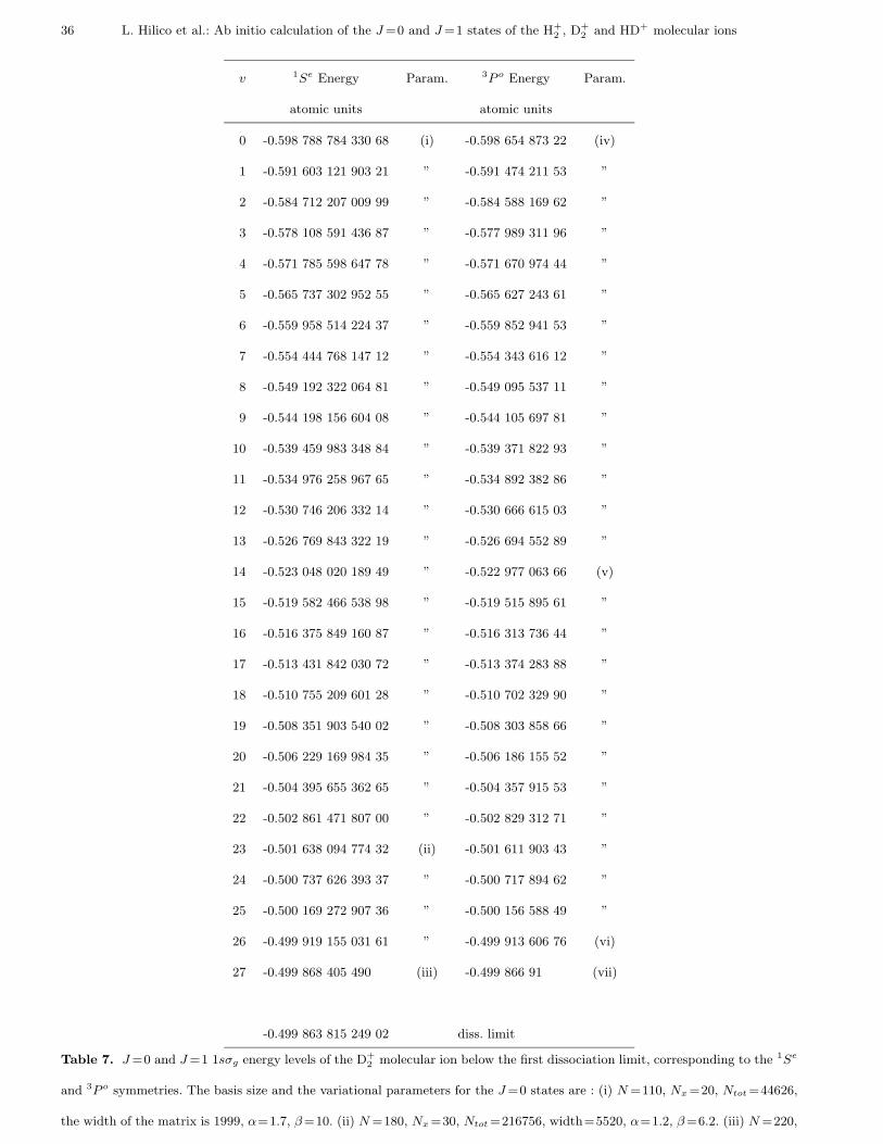
36 L. Hilico et al.: Ab initio calculation of the J =0 and J =1 states of the H+
2 , D+
2 and HD+ molecular ions
v 1Se Energy Param. 3P o Energy Param.
atomic units atomic units
0 -0.598 788 784 330 68 (i) -0.598 654 873 22 (iv)
1 -0.591 603 121 903 21 ” -0.591 474 211 53 ”
2 -0.584 712 207 009 99 ” -0.584 588 169 62 ”
3 -0.578 108 591 436 87 ” -0.577 989 311 96 ”
4 -0.571 785 598 647 78 ” -0.571 670 974 44 ”
5 -0.565 737 302 952 55 ” -0.565 627 243 61 ”
6 -0.559 958 514 224 37 ” -0.559 852 941 53 ”
7 -0.554 444 768 147 12 ” -0.554 343 616 12 ”
8 -0.549 192 322 064 81 ” -0.549 095 537 11 ”
9 -0.544 198 156 604 08 ” -0.544 105 697 81 ”
10 -0.539 459 983 348 84 ” -0.539 371 822 93 ”
11 -0.534 976 258 967 65 ” -0.534 892 382 86 ”
12 -0.530 746 206 332 14 ” -0.530 666 615 03 ”
13 -0.526 769 843 322 19 ” -0.526 694 552 89 ”
14 -0.523 048 020 189 49 ” -0.522 977 063 66 (v)
15 -0.519 582 466 538 98 ” -0.519 515 895 61 ”
16 -0.516 375 849 160 87 ” -0.516 313 736 44 ”
17 -0.513 431 842 030 72 ” -0.513 374 283 88 ”
18 -0.510 755 209 601 28 ” -0.510 702 329 90 ”
19 -0.508 351 903 540 02 ” -0.508 303 858 66 ”
20 -0.506 229 169 984 35 ” -0.506 186 155 52 ”
21 -0.504 395 655 362 65 ” -0.504 357 915 53 ”
22 -0.502 861 471 807 00 ” -0.502 829 312 71 ”
23 -0.501 638 094 774 32 (ii) -0.501 611 903 43 ”
24 -0.500 737 626 393 37 ” -0.500 717 894 62 ”
25 -0.500 169 272 907 36 ” -0.500 156 588 49 ”
26 -0.499 919 155 031 61 ” -0.499 913 606 76 (vi)
27 -0.499 868 405 490 (iii) -0.499 866 91 (vii)
-0.499 863 815 249 02 diss. limit
Table 7. J =0 and J =1 1sσg energy levels of the D+
2 molecular ion below the first dissociation limit, corresponding to the 1Se
and 3P o symmetries. The basis size and the variational parameters for the J =0 states are : (i) N =110, Nx =20, Ntot =44626,
the width of the matrix is 1999, α=1.7, β=10. (ii) N =180, Nx =30, Ntot =216756, width=5520, α=1.2, β=6.2. (iii) N =220,
Nx = 30, α = 0.9, β = 4. For the J = 1 states, they are : (iv) N = 54, Nx = 24, Ntot = 28850, width = 3054, α = 1.2, β = 19. (v)
N = 120, Nx = 20, Ntot = 130921, width = 9408, α = 1.7, β = 10. (vi) N = 140, Nx = 26, Ntot = 223731, width = 13294, α = 1.3,
β=7. (vii) N =140, Nx =26, α=1.1, β=5. All the digits shown in this table are converged.
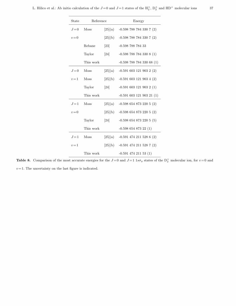
L. Hilico et al.: Ab initio calculation of the J =0 and J =1 states of the H+
2 , D+
2 and HD+ molecular ions 37
State Reference Energy
J =0 Moss [25](a) -0.598 788 784 330 7 (2)
v=0 [25](b) -0.598 788 784 330 7 (2)
Rebane [23] -0.598 788 784 33
Taylor [24] -0.598 788 784 330 8 (1)
This work -0.598 788 784 330 68 (1)
J =0 Moss [25](a) -0.591 603 121 903 2 (2)
v=1 Moss [25](b) -0.591 603 121 903 4 (2)
Taylor [24] -0.591 603 121 903 2 (1)
This work -0.591 603 121 903 21 (1)
J =1 Moss [25](a) -0.598 654 873 220 5 (2)
v=0 [25](b) -0.598 654 873 220 5 (2)
Taylor [24] -0.598 654 873 220 5 (5)
This work -0.598 654 873 22 (1)
J =1 Moss [25](a) -0.591 474 211 528 6 (2)
v=1 [25](b) -0.591 474 211 528 7 (2)
This work -0.591 474 211 53 (1)
Table 8. Comparison of the most accurate energies for the J =0 and J =1 1sσg states of the D+
2 molecular ion, for v=0 and
v=1. The uncertainty on the last figure is indicated.
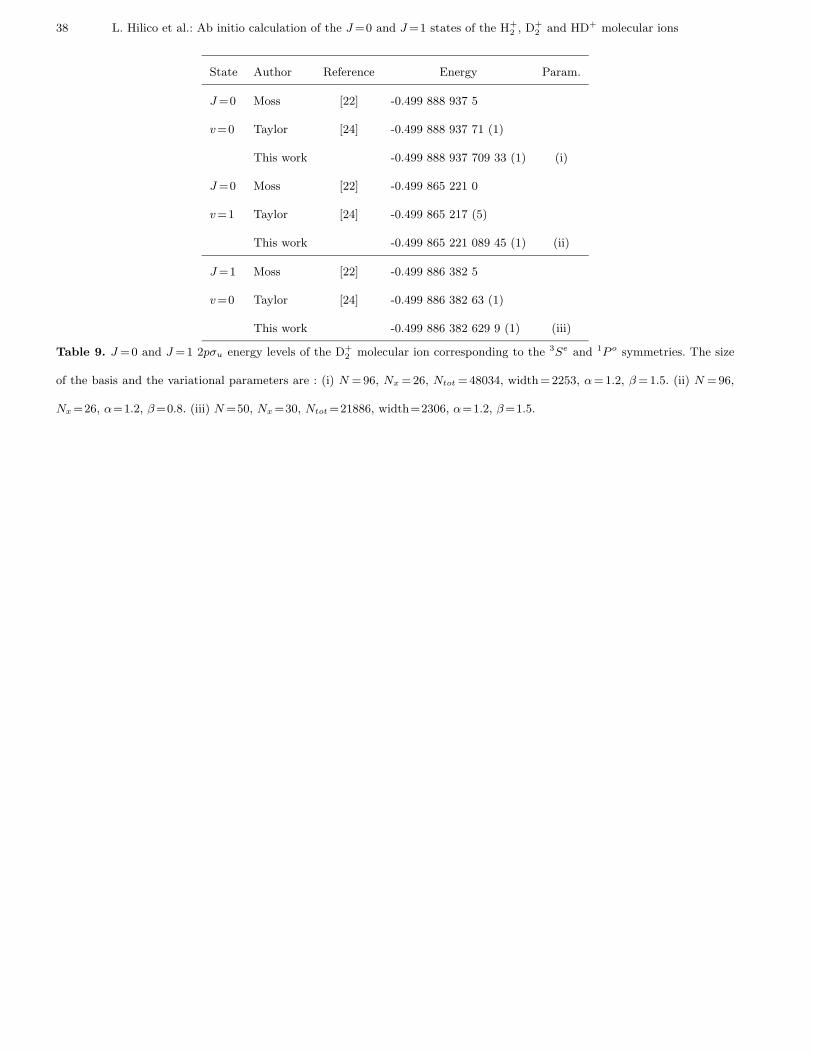
38 L. Hilico et al.: Ab initio calculation of the J =0 and J =1 states of the H+
2 , D+
2 and HD+ molecular ions
State Author Reference Energy Param.
J =0 Moss [22] -0.499 888 937 5
v=0 Taylor [24] -0.499 888 937 71 (1)
This work -0.499 888 937 709 33 (1) (i)
J =0 Moss [22] -0.499 865 221 0
v=1 Taylor [24] -0.499 865 217 (5)
This work -0.499 865 221 089 45 (1) (ii)
J =1 Moss [22] -0.499 886 382 5
v=0 Taylor [24] -0.499 886 382 63 (1)
This work -0.499 886 382 629 9 (1) (iii)
Table 9. J =0 and J =1 2pσu energy levels of the D+
2 molecular ion corresponding to the 3Se and 1P o symmetries. The size
of the basis and the variational parameters are : (i) N =96, Nx =26, Ntot =48034, width=2253, α=1.2, β =1.5. (ii) N =96,
Nx =26, α=1.2, β=0.8. (iii) N =50, Nx =30, Ntot =21886, width=2306, α=1.2, β=1.5.
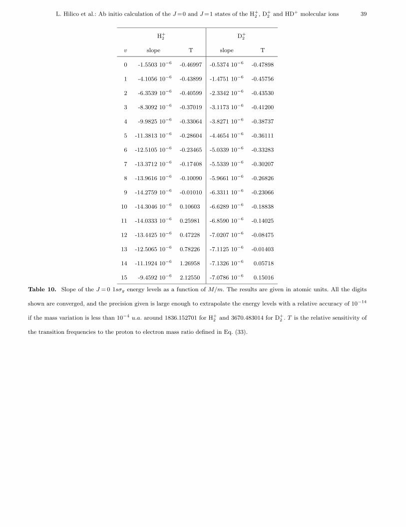
L. Hilico et al.: Ab initio calculation of the J =0 and J =1 states of the H+
2 , D+
2 and HD+ molecular ions 39
H+
2 D+
2
v slope T slope T
0 -1.5503 10−6 -0.46997 -0.5374 10−6 -0.47898
1 -4.1056 10−6 -0.43899 -1.4751 10−6 -0.45756
2 -6.3539 10−6 -0.40599 -2.3342 10−6 -0.43530
3 -8.3092 10−6 -0.37019 -3.1173 10−6 -0.41200
4 -9.9825 10−6 -0.33064 -3.8271 10−6 -0.38737
5 -11.3813 10−6 -0.28604 -4.4654 10−6 -0.36111
6 -12.5105 10−6 -0.23465 -5.0339 10−6 -0.33283
7 -13.3712 10−6 -0.17408 -5.5339 10−6 -0.30207
8 -13.9616 10−6 -0.10090 -5.9661 10−6 -0.26826
9 -14.2759 10−6 -0.01010 -6.3311 10−6 -0.23066
10 -14.3046 10−6 0.10603 -6.6289 10−6 -0.18838
11 -14.0333 10−6 0.25981 -6.8590 10−6 -0.14025
12 -13.4425 10−6 0.47228 -7.0207 10−6 -0.08475
13 -12.5065 10−6 0.78226 -7.1125 10−6 -0.01403
14 -11.1924 10−6 1.26958 -7.1326 10−6 0.05718
15 -9.4592 10−6 2.12550 -7.0786 10−6 0.15016
Table 10. Slope of the J = 0 1sσg energy levels as a function of M/m. The results are given in atomic units. All the digits
shown are converged, and the precision given is large enough to extrapolate the energy levels with a relative accuracy of 10−14
if the mass variation is less than 10−4 u.a. around 1836.152701 for H+
2 and 3670.483014 for D+
2 . T is the relative sensitivity of
the transition frequencies to the proton to electron mass ratio defined in Eq. (33).
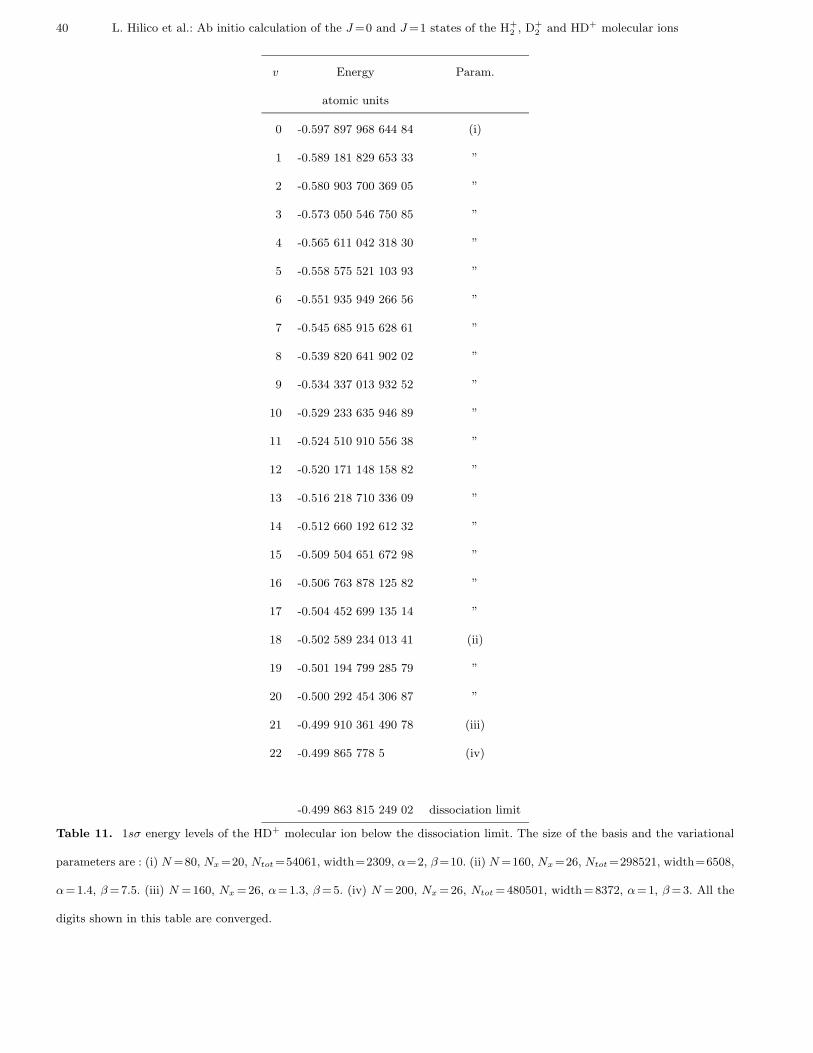
40 L. Hilico et al.: Ab initio calculation of the J =0 and J =1 states of the H+
2 , D+
2 and HD+ molecular ions
v Energy Param.
atomic units
0 -0.597 897 968 644 84 (i)
1 -0.589 181 829 653 33 ”
2 -0.580 903 700 369 05 ”
3 -0.573 050 546 750 85 ”
4 -0.565 611 042 318 30 ”
5 -0.558 575 521 103 93 ”
6 -0.551 935 949 266 56 ”
7 -0.545 685 915 628 61 ”
8 -0.539 820 641 902 02 ”
9 -0.534 337 013 932 52 ”
10 -0.529 233 635 946 89 ”
11 -0.524 510 910 556 38 ”
12 -0.520 171 148 158 82 ”
13 -0.516 218 710 336 09 ”
14 -0.512 660 192 612 32 ”
15 -0.509 504 651 672 98 ”
16 -0.506 763 878 125 82 ”
17 -0.504 452 699 135 14 ”
18 -0.502 589 234 013 41 (ii)
19 -0.501 194 799 285 79 ”
20 -0.500 292 454 306 87 ”
21 -0.499 910 361 490 78 (iii)
22 -0.499 865 778 5 (iv)
-0.499 863 815 249 02 dissociation limit
Table 11. 1sσ energy levels of the HD+ molecular ion below the dissociation limit. The size of the basis and the variational
parameters are : (i) N =80, Nx =20, Ntot =54061, width=2309, α=2, β=10. (ii) N =160, Nx =26, Ntot =298521, width=6508,
α=1.4, β =7.5. (iii) N =160, Nx =26, α=1.3, β =5. (iv) N =200, Nx =26, Ntot =480501, width=8372, α=1, β =3. All the
digits shown in this table are converged.


![[J. Res. Natl. Inst. Stand. Technol. 105 Ab Initio Values ... · [J. Res. Natl. Inst. Stand. Technol. 105, 667–688 (2000)] Ab Initio Values of the Thermophysical Properties of Helium](https://img.pdfslide.net/doc/110x75/5f2f5982e8ee966446353fc4/j-res-natl-inst-stand-technol-105-ab-initio-values-j-res-natl-inst.jpg)