Embed Size (px)
Citation preview

AN ABSTRACT OF THE THESIS OF
Abel Forest Brumo for the degree Master of Science in Fisheries Science presented on September 22, 2006. Title: Spawning, Larval Recruitment, and Early Life Survival of Pacific Lampreys in the South Fork Coquille River, Oregon
Abstract approved:
_______________________________________________________________ Douglas F. Markle
Recently, there has been concern over the decline of the Pacific lamprey,
Lampetra tridentata, in the northwestern United States. However, effective management
has been impeded by data gaps in basic biology, especially in the early life stages.
Consequently, in 2004 and 2005 I examined reproductive ecology, larval recruitment, and
lamprey monitoring methods in the South Fork Coquille River, a coastal Oregon stream.
In Chapter 2 I monitored spawning populations at large (9.2 km) and small (focal
area) scales. Relationships between adult counts at the two spatial scales and adult and
redd counts at the large scale were analyzed. Weekly adult, redd, and carcass counts and
tagging were also used to describe spawning and residence times, movement, size, and
sex of mature adults. Large-scale adult and redd counts were highly correlated (2004, r2 =
0.867; P = 0.0069; 2005, r2 = 0.877; P = 0.0002); as were large-scale and focal area adult
counts over both years combined (r2 = 0.690, P = 0.0001) and in 2004 (r2 = 0.753, P =
0.0250), but not in 2005 when densities were much lower (r2 = 0.065, P = 0.5069).
Average residence time in spawning areas was less than a week for males and shorter for
DWR 1129

females, since >90% of recaptured fish were male. Two-thirds of dead fish (2:1) were
male, versus only one-half of live fish (1:1), indicating additional sex-specific differences
in postspawning behavior. No seasonal or spatial patterns in sex ratio or adult length were
detected. Both adult and redd counts have inherent errors related to observer variability,
movement during surveys, night spawning, and variable visibility due to weather and
flow. To make adult and redd counts more useful for population monitoring their errors
need to be better quantified and their relevance to life-cycle dynamics better understood.
In Chapter 3 I monitored intra-annual cohorts of spawning adults and emergent
larvae at a single spawning area to examine annual and seasonal patterns of spawning,
larval recruitment, and early life survival. In 2004 spawning occurred from April 6–June
3 (59 d) and larval emergence occurred from May 6–June 28 (54 d). In 2005 both
spawning and emergence were later and more protracted, from April 25–July 3 (70 d) and
May 15–July 25 (71 d), respectively. Over both years, larval recruitment was highly
variable and only marginally correlated with spawning stock (r2 = 0.149, P = 0.0512).
Survival until larval emergence was significantly related to spawning stock size,
discharge during spawning, and their interaction. Survival generally declined with
increasing spawning stock and decreasing discharge, both apparently related to negative
density-dependent effects, which resulted in highly variable early life survival. For
example, in April 2004, 65% of larvae were produced by 28% of spawners, while in
May, 35% of larvae were produced by 70% of spawners. Egg predation by speckled dace,
Rhinichthys osculus, increased with temperature, but contrary to expectations, had no
detectable effect on survival until emergence.

This study provided justification for a multi-life stage approach to monitoring
Pacific lamprey populations and understanding their dynamics. Application of this
approach can provide insight into density-dependent survival and the roles of biotic and
abiotic factors in larval production. Applied to the South Fork Coquille, Pacific lamprey
larval production appeared to have an upper limit related, in part, to spawner density.

©Copyright by Abel F. Brumo September 22, 2006 All Rights Reserved

Spawning, Larval Recruitment, and Early Life Survival of Pacific Lampreys in the South Fork Coquille River, Oregon
by
Abel F. Brumo
A THESIS
submitted to
Oregon State University
in partial fulfillment of the requirements for the
degree of
Master of Science
Presented September 22, 2006 Commencement June 2007

Master of Science thesis of Abel F. Brumo presented on September 22, 2006.
Approved:
Major Professor, representing Fisheries Science
Head of the Department of Fisheries and Wildlife
Dean of the Graduate School
I understand that my thesis will become part of the permanent collection of Oregon State University libraries. My signature below authorizes the release of my thesis to any reader upon request.
Abel F. Brumo, Author

ACKNOWLEDGMENTS
First and foremost, I want to thank my advisor Doug Markle, who initially
provided me with the opportunity to carry out this research. Doug’s vast understanding
of aquatic ecology, systematics, and fisheries management, along with his ability to
teach, have greatly increased my appreciation for the intricacy of the natural world. At
the same time, his hands-off approach has unquestionably encouraged my development
as an independent researcher. My colleagues in the Markle Lab deserve recognition as
well: Dave Simon, Mark Terwilliger, Stacy Remple, Jess Kettratad, and Sue Reithel,
have all helped make my time at Oregon State University educational and enjoyable in
various ways.
I am very appreciative of support received from Guillermo Giannico, who, in
addition to offering useful advice, played a significant role in my decision to attend OSU.
From the beginning, Guillermo has been more than willing to listen to my ideas, while
offering invaluable career guidance. Likewise, I want to thank Virginia Lesser for her
willingness to be on my committee and for her statistical advice.
I am especially grateful for the assistance of Leo Grandmontagne and Steve
Namitz (USDA Forest Service—Powers Ranger District), whose great knowledge of the
Coquille Basin, field assistance, and gear engineering were priceless in the success of this
project. Leo and his girlfriend Terry and Steve and his family also offered a great deal of
hospitality and comic relief during my time in Powers. I also appreciate the friendliness
and hospitality of the entire Powers Ranger District staff.
I am equally thankful for the full support of ODFW District Biologist Mike Gray.
Mike Meeuwig and Jennifer Bayer provided valuable data on and insight into lamprey

early life history and development. Both Stephanie Gunckel and Stewart Reid offered
useful advice during the formulation of my project ideas. Kim Jones, Steve Jacobs, Doug
Young, and Doug Baus assisted with procurement of project funding. Thanks to Brian
Riggers for loaning a pontoon boat to the project in 2004. In 2005 Dustin Thompson
provided assistance with spawning surveys, while Brian Alfonse and Mark Jansen helped
with larval measurement. Many others in the Fisheries and Wildlife Department at OSU,
as well as in the Northwest fisheries community, have offered support and/or useful
guidance.
Additionally, I am grateful for my friends around the world, who have been
supportive throughout the process—especially my brother Aaron, who has always been
encouraging when times were tough. My local fishing, basketball, and poker companions
also deserve many thanks for ensuring that I escaped from my office on a sufficient basis,
and of course, for their intensely stimulating and sophisticated conversations during our
travels.
Most of all, I owe enormous gratitude to parents who have fostered my
fascination for the natural world and encouraged my development as a scientist from a
young age. Although not trained in natural sciences, they both have a deep appreciation
for natural history and have shown a great deal of interest in this project.
This work was supported by Oregon Department of Fish and Wildlife and United
States Fish and Wildlife Service. Specimen collections were authorized under a series of
Oregon scientific taking permits through OR2004-1365 and OR2005-2310, and an OSU
Institutional Animal Care and Use permit LAR-ID 2926.

CONTRIBUTION OF AUTHORS
Steve Namitz and Leo Grandmontagne assisted with study design and data collection for
Chapter 2. Dr. Douglas Markle assisted with data analysis and interpretation of Chapters
2 and 3.

TABLE OF CONTENTS
Page
CHAPTER 1. GENERAL INTRODUCTION .................................................................. 1
STUDY LOCATION...................................................................................................... 4 PACIFIC LAMPREY LIFE HISTORY ......................................................................... 6
CHAPTER 2. PATTERNS OF PACIFIC LAMPREY SPAWNING TIME, LENGTH, AND SEX-RATIO IN A COASTAL OREGON STREAM: IMPLICATIONS FOR MONITORING................................................................................................................... 7
INTRODUCTION .......................................................................................................... 7 METHODS ................................................................................................................... 10
Study site................................................................................................................... 10 Abiotic variables ....................................................................................................... 10 Large-scale surveys................................................................................................... 11 Focal area surveys..................................................................................................... 12
RESULTS ..................................................................................................................... 13
Abiotic variables ....................................................................................................... 13 Large-scale adult counts ........................................................................................... 13 Large-scale carcass recovery .................................................................................... 14 Adult vs. redd counts ................................................................................................ 14 Focal area adult counts.............................................................................................. 15 Large-scale vs. focal adult counts............................................................................. 16 Tagging recaptures, residence time, and movement................................................. 16 Adult length .............................................................................................................. 17 Sex ratio .................................................................................................................... 18 Spawning and ecological observations ..................................................................... 18 Western brook lamprey............................................................................................. 19
DISCUSSION............................................................................................................... 20
Adult counts and spawning time............................................................................... 20 Adult vs. redd counts ................................................................................................ 21 Spatial scale in adult counts...................................................................................... 24 Tagging recaptures, residence time, and movement................................................. 25 Adult length .............................................................................................................. 27 Sex ratio .................................................................................................................... 29 Western brook lamprey............................................................................................. 30 Conclusions............................................................................................................... 31
TABLES ....................................................................................................................... 33 FIGURES...................................................................................................................... 37

TABLE OF CONTENTS (Continued)
Page
CHAPTER 3. ANNUAL AND INTRA-ANNUAL PATTERNS IN PACIFIC LAMPREY SPAWNING, LARVAL RECRUITMENT, AND EARLY LIFE SURVIVAL IN A COASTAL OREGON STREAM....................................................... 47
INTRODUCTION ........................................................................................................ 47 METHODS ................................................................................................................... 52
Sampling site............................................................................................................. 52 Abiotic variables ....................................................................................................... 52 Spawning activity...................................................................................................... 53 Larval production...................................................................................................... 53 Egg predation ............................................................................................................ 57 Data analyses ............................................................................................................ 58
RESULTS ..................................................................................................................... 66
Abiotic variables ....................................................................................................... 66 Spawning activity...................................................................................................... 67 Larval production...................................................................................................... 68 Diel periodicity in larval drift ................................................................................... 71 Stock – recruitment ................................................................................................... 71 Survival until larval emergence ................................................................................ 72
DISCUSSION............................................................................................................... 76
Spawning activity...................................................................................................... 76 Larval production...................................................................................................... 78 Stock-recruitment and early survival ........................................................................ 82 Conclusions............................................................................................................... 91
TABLES………………………………………………………………………………94
FIGURES...................................................................................................................... 98
CHAPTER 4. SUMMARY AND CONCLUSIONS..................................................... 113
LITERATURE CITED ................................................................................................... 116
APPENDICES ................................................................................................................ 125

LIST OF FIGURES Figure Page
2.1 Location of the large-scale survey section, study reaches, and the focal area within the Coquille River Basin, Oregon.…………………………..... 37
2.2 2004 and 2005 discharge (cubic feet per second) on South Fork Coquille
River from January 1 to July 30………...………………………………… 38
2.3 Daily mean water temperature at the focal area from April 4 until August 3, 2004 and 2005…………….……………………………………………. 38
2.4 Number of live adult male and female Pacific lampreys observed on
spawning areas during 2004 large-scale surveys (all reaches combined)… 39
2.5 Number of live adult male and female Pacific lampreys observed on spawning areas during 2005 large-scale surveys (all reaches combined). Stars represent surveys in which zero fish were seen. Note difference in scale of y-axis between Figures 2.4 and 2.5……………………………… 39
2.6 Number of carcasses recovered in large-scale reaches during 2004
surveys. Reaches are ordered from upstream (Whiskey) to downstream (Yellow)………………………………………………............................... 40
2.7 Number of carcasses recovered in large-scale reaches during 2005
surveys. Reaches are ordered from upstream (Whiskey) to downstream (Yellow)…………………………………………………………………… 40
2.8 Number of Pacific lamprey redds counted during 2004 large-scale
surveys (all reaches combined)…………………………………………… 41
2.9 Number of Pacific lamprey redds counted during 2005 large-scale surveys (all reaches combined)…………………………………………… 41
2.10 Number of redds counted versus number of live adult Pacific lampreys
captured during weekly large-scale surveys………………………………. 42
2.11 Number of redds counted per adult versus days from the first adult was observed in large-scale surveys. A 5/27/04 observation of one fish and 73 redds, 28 days from the first adult observation, was omitted………….. 42
2.12 Seasonal distribution of adult Pacific lampreys in the focal area in 2004.
The arrow indicates a period of high discharge when sampling was not possible. Stars represent observations when zero fish were seen……........ 43

LIST OF FIGURES (Continued) Figure Page2.13 Seasonal distribution of adult Pacific lampreys in the focal spawning area
in 2005. Arrows indicate periods of high discharge when sampling was not possible. Stars represent observations when zero fish were seen. Note the difference in y-axis scale between Figures 2.12 and 2.13…...….. 43
2.14 Weekly mean focal adult counts (fish per observation) versus number of
live adult Pacific lampreys captured during weekly large-scale surveys…. 44
2.15 Length frequencies of male and female mature adult Pacific lampreys sampled in 2004 and 2005 (live fish and carcasses included)….…………. 44
2.16 Mean lengths of live mature adult Pacific lampreys collected from
spawning areas on large-scale survey dates when fish were measured in 2004 and 2005. No males were measured on May 27, 2004 and no females were measured on June 15, 2005. Bars represent Bonferroni intervals from multiple comparison procedures. There were no statistically significant differences in length between any of the spawning groups in either year, except for females between April 28 and May 25, 2005……………………………………………………………………….. 45
2.17 Sex ratio of live adult Pacific lampreys on spawning grounds versus days
since the first mature adult was observed in 2004 and 2005 large-scale surveys.…………………………................................................................. 45
2.18 Number of mature western brook lampreys observed in the focal area in
2004 and 2005. Zeros denote observations in which no fish were counted.………………………………………………………………….... 46
3.1 Location of focal spawning area in relation to the large-scale survey section (see Chapter 2) and the Coquille River Basin, Oregon…………… 98
3.2 2004 and 2005 discharge (cubic feet per second) on South Fork Coquille
River from January 1 to July 30……………………………………...…… 99
3.3 Daily mean water temperature at the focal area from April 4 until August 3, 2004 and 2005…………………………………………………….……. 99
3.4 Seasonal distribution of adult Pacific lampreys in the focal spawning area
in 2004. The arrow indicates a period of high discharge when sampling was not possible. Stars represent observations when zero fish were seen………………………………………………………………….…….. 100

LIST OF FIGURES (Continued) Figure Page
3.5 Seasonal distribution of adult Pacific lampreys in the focal spawning area in 2005. Arrows indicate periods of high discharge when sampling was not possible. Stars represent observations when zero fish were seen. Note the difference in y-axis scale between Figures 3.4 and 3.5………..... 100
3.6 Number of mature adult Pacific lampreys observed on the focal area
versus daily mean water temperature in 2004 and 2005………………….. 101
3.7 Number of mature adult Pacific lampreys counted on the focal area versus daily mean discharge during observations in 2004 and 2005..……. 101
3.8 Age-0 lamprey drift rates in 2004 and 2005 for emergent ammocoetes (8–
9 mm), ammocoetes greater than 9 mm, and those less than 8 mm. Note the difference in the y-axis scale between years………………………….. 102
3.9 Loge 8–9 mm larval drift rate (number per minute) versus mean water
temperature during development………………………………………….. 103
3.10 Seasonal production of emergent larvae (number per minute) and mean water temperature and discharge during corresponding developmental periods in 2004 and 2005……………...………………………………….. 104
3.11 Loge 8–9 mm larval drift rate (number per minute) versus mean discharge
during development….……………………………………………………. 105
3.12 Percent drift density at each net time for age-0 ammocoetes captured during diel samples averaged over 6 sampling cycles; 2004 and 2005 samples combined. Bars represent standard errors……………………….. 105
3.13 Relationship between larval production (8–9 mm ammocoete drift rate)
and spawning stock (adult count estimates from corresponding spawning period)……………………………………………………………………... 106
3.14 Percent of 2004 emergent larval production collected during drift samples
overlaid on percent of annual adult observations from corresponding spawning periods. Differences between magnitude of percent adults and percent emergent larvae represent relative survival until emergence…….. 107
LIST OF FIGURES (Continued) Figure Page3.15 Percent of 2005 emergent larval production collected during drift samples
overlaid on percent of annual adult observations from corresponding spawning periods. Differences between magnitude of percent adults and percent emergent larvae represent relative survival until emergence…….. 107
3.16 Relationship between relative survival until emergence (emergent larval
drift rate per corresponding adult) and mean discharge during the spawning period (r2 = 0.307; P = 0.0033; N = 26).……………………….. 108
3.17 Relationship between survival until emergence (emergent larval drift rate
per corresponding adult) and number of adults present in the corresponding spawning period (r2 = 0.252; P = 0.0091; N = 26)………... 108
3.18 Relationship between relative survival until emergence (emergent larval
drift rate per corresponding adult) and mean water temperature during the spawning period…………………………………………………………… 109
3.19 Comparison of mean discharge during spawning between the highest
50% (N=13) and lowest 50% (N=13) of intra-annual larval cohort survival values………..…………………………………………………… 109
3.20 Comparison of spawning stock between the highest 50% (N=13) and
lowest 50% (N=13) of intra-annual larval cohort survival values………... 110
3.21 Examples of speckled dace feeding behavior. The photograph on the left illustrates an individual dace burrowing into redd gravels in search of lamprey eggs. The photo on the right was taken immediately downstream of a recently spawned-in Pacific lamprey redd………............ 111
3.22 Photographic documentation of high densities of speckled dace preying
on eggs during Pacific lamprey spawning. Each white arrow represents a visible, individual dace (N = 76). The area in the photograph is approximately 1 m2………………………………………………………... 111
3.23 Monthly means and standard errors of speckled dace relative feeding
level during 2004 and 2005 Pacific lamprey spawning periods…………... 112

LIST OF TABLES Table Page
2.1 Dates of large-scale adult and redd surveys in 2004 and 2005……………. 33
2.2 Reach information for large-scale surveys, ordered from upstream to downstream (9.2 km total)………………………………………………… 33
2.3 Abundance (N) and mean length of live and dead Pacific lampreys during
2004 and 2005 large-scale surveys; excluding live fish seen but not captured (54 in 2004 and 31 in 2005)….………………………………….. 34
2.4 Total number of live adult Pacific lampreys per reach and number per
total kilometer surveyed for 2004 and 2005 large-scale surveys. Reaches are ordered from upstream to downstream………………………………... 34
2.5 Total number of Pacific lamprey redds per reach and number per total
kilometer surveyed for 2004 and 2005 large-scale surveys. Reaches are ordered from upstream to downstream...………………………………….. 34
2.6 Matrix of r2 statistics and associated P-values for relationships between
weekly adult Pacific lamprey counts in each of the large-scale survey reaches, the entire large-scales section, and the focal area (combined 2004 and 2005 data; N = 15 for all survey types). Survey reaches are ordered from upstream to downstream…………………………………………….. 35
2.7 Number and mean lengths (cm) of tagged Pacific lampreys recaptured or
recovered dead from large-scale surveys in 2004…………………………. 35
2.8 Tagging and recovery locations and weeks, and movement distance and direction for live Pacific lampreys recaptured during 2004 weekly large-scale surveys………………………………………………………………. 36
2.9 Numbers and percent of Pacific lampreys from each tagging date
recaptured on spawning grounds alive after one week in 2004; note that a female recaptured after only one day is excluded. Zero fish were recaptured in 2005………………………………………………………… 36
3.1 Calculation of mean effective degree days (EDD) until the larval stage
(stage 18, see Piavis 1961) from laboratory data on Pacific lamprey eggs reared at four constant temperatures………………………………………. 94
3.2 Variables employed in simple and multiple linear regression models
explaining loge larval drift rate per adult (survival until emergence) for intra-annual cohorts and associated symbols………………….…………... 94

LIST OF TABLES (Continued) Table
Page
3.3 Total number of age-0 ammocoetes caught at focal area in biweekly and diel samples by size class in 2004 and 2005; N = number of net samples. Net samples from small nets consisted of two small nets stacked to cover the water column……………………...…………………………………… 95
3.4 Relative annual survival until the larval phase for Pacific lampreys in
2004 and 2005. Total Annual Larval Production equals the annual sum of emergent ammocoete drift rates from all biweekly nets. Number of Spawners is the estimated number of mature adults present in the focal area during spawning periods corresponding to biweekly larval cohorts. Relative Survival Index equals Total Annual Larval Production divided by Number of Spawners.……………………………………………………… 95
3.5 Percent of Pacific lampreys spawning in each month, percent of larval
production resulting from each month’s spawners, and monthly index of survival (calculated by dividing percent of larvae by percent of spawners) for 2004 and 2005. Within each year, index of survival values greater than 1.0 are considered above average and lower than 1.0 below average... 95
3.6 Results of simple linear regression models explaining survival until
emergence (loge larval drift rate per adult; df = 25). Note: r2 values and coefficient values are only listed for models with P < 0.15. See Table 3.1 for description of variable symbols………………………………………... 96
3.7 Comparison of mean values of explanatory variables between the highest
50% (N=13) and lowest 50% (N=13) of intra-annual-cohort survival values from 2004 and 2005 combined data. P-values were derived from two sample t-tests. See Table 3.1 for description of variable symbols…… 96
3.8 Top ten linear regression models describing relative Pacific lamprey
survival until emergence; selected from AICc analysis. Akaike weight was calculated from all 145 candidate models (N = 26 for all models)…… 97
3.9 Relative importance values of variables used to predict survival until
emergence. Calculated from Akaike weights of the 145 candidate models……………………………………………………………………... 97

LIST OF APPENDICES
Appendix Page I Methods, Results, and Discussion from an in situ egg incubation pilot
project………………………………………………………………….. 126
II Length frequency of age one and older (>18 mm) ammocoetes collected in biweekly and diel nets set below the focal area (2004: N = 230, 2005: N = 672). Samples could consist of both western brook and Pacific lampreys, but are likely dominated by the latter………....... 129
III Scatter plot of age one and older (>18 mm) ammocoete lengths across
2004 and 2005 sampling seasons from biweekly and diel drift net samples……………..………………………………………………….. 129
IV Actual and estimated focal area adult counts in 2004. Triangles
represent dates in which daily mean water temperature was <11°C and spawning activity was assumed to be zero; asterisks are points estimated using linear interpolation between adjacent points; and crosses are temperature-predicted regression estimates…..…………… 130
V Actual and estimated focal area adult counts in 2005. Triangles
represent dates in which daily mean water temperature was <11°C and spawning activity was assumed to be zero; asterisks are points estimated using linear interpolation between adjacent points; and crosses are temperature-predicted regression estimates……..………… 130
VI Correlation coefficients (top) and P-values (bottom) of explanatory
variables used in multiple linear regression models explaining relative survival until emergence. Results are for 2004 and 2005 data combined. See Table 3.1 for description of variable symbols…………….…………………………………………………... 131

CHAPTER 1
GENERAL INTRODUCTION
The Pacific lamprey, Lampetra tridentata, is a culturally and ecologically
important, anadromous fish that spawns and rears in Northern Hemisphere streams
flowing into the temperate Pacific Ocean (Hubbs and Potter 1971; Byram 2002; Close et
al. 2002; Close et al. 2004; Peterson 2006). In recent years, state, federal, and tribal
agencies have expressed concern at the apparent decline of lamprey populations in the
Northwestern United States (Close et al. 2002, Moser and Close 2003; CRBLTW 2005;
ODFW 2006). Widespread anecdotal accounts of decreased Pacific lamprey spawning
and carcasses have been supported by a substantial reduction in counts of migrating
individuals at dams since the late 1960’s (Moser and Close 2003; Nawa 2003).
The root causes of lamprey population decline are unknown, but in all likelihood,
multifaceted. Due to similarity in habitat requirements and life histories between the
Pacific lamprey and anadromous salmonids, as well as a near parallel in population
collapse, it is likely that many of the same factors are limiting their survival. Dewatering
of streams, obstruction of migration routes, predation by non-indigenous species,
degradation of spawning and rearing habitats, and changes in ocean conditions, among
others, have been theorized as sources of lamprey decline (Moser et al. 2002; Close et al.
2003, Nawa 2003, ODFW 2006).
A 2003 petition by twelve conservation organizations for Endangered Species Act
(ESA) protection of four western United States lamprey species, including Pacific
lamprey and western brook lamprey, L. richardsoni, galvanized region-wide efforts to

2
improve understanding of the biology and status of these fishes (Nawa 2003). Although
the United States Fish and Wildlife Service (USFWS) halted species status review in a
Dec. 27, 2004 "90-day-finding" (U.S. Office of the Federal Register 2004), efforts to list
Pacific lamprey are anticipated to resume in the future. Meanwhile, the status of this
species remains a concern to Native American tribes, conservation organizations, and
state, federal, and tribal scientists across the region.
There have been several comprehensive investigations of Pacific lamprey biology
(Pletcher 1963; Kan 1975; Beamish 1980; Beamish and Levings 1991), plus a concerted
effort in recent years to improve our understanding of freshwater distribution (Graham
and Brun 2005; Luzier and Silver 2005; Cochnauer et al. 2006), habitat (Torgersen and
Close 2004; Gunckel et al. 2006), migration timing (van de Wetering 1998; Bayer et al.
2000), dam passage (Moser et al. 2002), phylogeny and stock-structure (Docker et al.
1999; Goodman et al. 2006), and status (Close et al. 1995; Kostow 2002; Moser and
Close 2003). Despite these recent advances, effective management and recovery
continue to be hindered by a lack of basin-specific information on distribution, life-
history, population dynamics, and factors limiting survival (Kostow 2002; Moser and
Close 2003; CRBLTW 2005; ODFW 2006). Most research has taken place in the
Columbia River Basin, with little targeted research elsewhere. Furthermore, information
on the egg incubation period and early larval stages is especially scarce: with few
exceptions (Meeuwig et al. 2005), research on Pacific lamprey has focused on adults,
juvenile outmigrants, and older size-classes of larvae.
Understanding biotic and abiotic factors controlling survivorship and recruitment
of early larvae is a key element in successful fisheries management and recovery (Houde

3
1987; Magnuson 1991; Pepin 2002). Because mortality rates of fish eggs and larvae are
naturally high and variable, survival during these stages is especially important in
shaping eventual adult recruitment (Hjort 1914; Rice et al. 1987; Leggett and DeBlois
1994; Johnston et al. 1995; Houde 2002; Pepin 2002). Recruitment level is initially
dependent on the number of spawning adults, but other factors such as predation, disease,
and starvation can obscure that relationship and ultimately be more important in
determining recruitment (Elliot 1989; Leggett and DeBlois 1994; Houde 2002).
A fundamental step in evaluating recruitment limitations and understanding
population dynamics, especially in a species as little-studied as the Pacific lamprey, is
collection of clear and consistent data on spawning populations. In most river basins,
however, there is an absence of reliable annual monitoring data (Kostow 2002). Until
recently, the primary means for monitoring lamprey populations has been counts of
upstream migrants at mainstem dams (Kostow 2002; Moser and Close 2003). Because
these surveys are designed for monitoring salmonids, they have inherent weaknesses
when used for lampreys (Moser and Close 2003). Although they can be useful for
evaluating long term population trends, dam counts do not provide information on when
or where passing fish will spawn.
Adult and redd counts on spawning grounds offer more accurate data on timing
and spatial distribution of spawners, but the majority of these data are collected
irregularly or are incidental to steelhead monitoring (Kostow 2002). Implementation of
standardized monitoring protocols is necessary to fully comprehend the meaning of
spawning survey data. Likewise, knowledge on spatial and temporal patterns in
spawning activity, sex ratio, length frequency, and the relationship between adults and

4
redds is imperative for accurate interpretation of spawning survey data, as well as for
understanding patterns in larval recruitment.
The overall goal of this study was to describe Pacific lamprey reproductive
ecology and larval recruitment patterns in a Northwest coastal river system—with an
emphasis on assessment of monitoring methods. Both spawning adult and emergent
larval populations were monitored regularly on the South Fork Coquille River during
2004 and 2005 spawning seasons. Chapter 2 evaluates the utility of adult and redd counts
for gauging spawning activity; compares timing of spawning on small and larger spatial
scales; and documents temporal and spatial trends in length frequency and sex ratio of
spawning adults in relation to interpretation of monitoring data. Chapter 3 describes
variation in spawning time and larval production between and within years; evaluates the
relationship between spawning stock and larval production; and documents and describes
potential limitations to early life survival. Chapter 4 presents a summary of findings as
they relate to species management and future research needs.
STUDY LOCATION
The river name “Coquille” is thought to be derived from the Chinook Jargon (a
widely used trade language across the Northwest) words “scoquel” or “coquel,” meaning
eel, which is a commonly used vernacular term for Pacific lamprey (Byram 2002). This
name, along with historical accounts and interviews with tribal elders from the area,
suggest that Pacific lampreys were once extremely abundant in the basin and one of the
most important trade items for the Coquille Indians (Byram 2002).

5
At 2743 km2, the Coquille River Basin is the largest river system originating in
Oregon’s coastal range. The South Fork Coquille River is a 4th order stream originating
in the Rogue-Siskiyou National Forest and draining roughly 746 km2, or 27% of the
Coquille catchment area. The annual discharge pattern is typical of a Northwest coastal
river system, with peak flows in winter and minimum flows in late summer. Mean
monthly discharges for the South Fork Coquille River for January, April, and August
from 1917–2004 were 1808±107.6 cfs, 918± 55.1 cfs, and 35±1.5 cfs, respectively
(mean±SE; USGS gauge # 14325000 at river km 105.4). A flashy system, the South
Fork Coquille is subject to rapid, order of magnitude changes in discharge during the
early portion of Pacific lamprey spawning season.
In addition to Pacific and western brook lampreys, native fish species present in
the Coquille River include: speckled dace (Rhinichthys osculus), largescale sucker
(Catostomus macrocheilus), three-spined stickleback (Gasterosteus aculeatus), prickly
sculpin (Cottus asper), coastrange sculpin (C. aleuticus), riffle sculpin (C. gulosus),
reticulate sculpin (Cottus perplexus), coho salmon (Oncorhynchus kisutch), chinook
salmon (O. tshawytscha), winter steelhead (O. mykiss), and coastal cutthroat trout (O.
clarki clarki). Known non-indigenous species, found primarily in lower gradient reaches
near the mainstem Coquille River, include yellow bullhead (Ameiurus natalis),
largemouth bass (Micropterus salmoides), striped bass (Morone saxatilis) and American
shad (Alosa sapidissima).

6
PACIFIC LAMPREY LIFE HISTORY Pacific lamprey spawning can take place from March through July depending on
water temperature and the river system (Pletcher 1963; Kan 1975). During spawning,
eggs are deposited into a gravel redd where they hatch after approximately 15 days and
spend another 15 days until they emerge into the drift at night. These eyeless larvae, or
ammocoetes, settle out and burrow into downstream depositional areas, in which they
spend a protracted filter-feeding larval phase (4–10 years) prior to undergoing
metamorphosis into an eyed adult (Pletcher 1963; Moore and Mallatt 1980; van de
Wetering 1998). After metamorphosis, these smolt-like individuals, or macropthalmia,
migrate to the ocean between fall and spring to feed parasitically on marine fishes
(Richards and Beamish 1981; Beamish and Levings 1991; van de Wetering 1998).
Pacific lampreys are thought to remain in the ocean for approximately 18–40 months
before returning to freshwater as immature adults between April and July on the Oregon
coast and in southwestern Canada (Kan 1975; Beamish 1980). In the Klamath and
Columbia rivers, they have been reported to enter freshwater year round (Kan 1975;
Larson and Belchik 1998). After remaining inactive under boulders or similar substrate
throughout the winter (Bayer et al 2000) Pacific lampreys come out the following spring
as sexually mature adults to spawn. Like Great Lakes sea lampreys, Petromyzon
marinus, Pacific lampreys do not necessarily home to natal spawning streams (Bergstedt
and Seelye 1995; Goodman et al. 2006). Instead, it is thought that migratory lamprey
species select spawning location based on presence and concentration of a pheromone-
like substance secreted by ammocoetes (Bjerselius et al. 2000; Vrieze and Sorensen
2001).

7
CHAPTER 2
PATTERNS OF PACIFIC LAMPREY SPAWNING TIME, LENGTH, AND SEX-
RATIO IN A COASTAL OREGON STREAM: IMPLICATIONS FOR MONITORING
INTRODUCTION
There have been several comprehensive investigations of the Pacific lamprey,
Lampetra tridentata, in the Northwestern United States (Kan 1975) and British Columbia
(Pletcher 1963; Beamish 1980; Beamish and Levings 1991), yet there is little basin-
specific information on their life history, distribution, and basic biology (CRBLTW
2005). Due to the diversity in size, climate, and ecology among river systems in the
Pacific lamprey’s expansive range, there is potential for geographic variation in life
history, ecological roles, and demographic processes. Successful management and
protection of this species requires documentation and better understanding of such
geographic differences.
Since a proposed Endangered Species Act (ESA) listing in 2003 (Nawa 2003),
most Pacific lamprey research and management activities have occurred within the
Columbia River Basin (Torgersen and Close 2004; CRBLTW 2005; Graham and Brun
2005; Howard et al. 2005; Luzier and Silver 2005; Meeuwig and Bayer 2005; Meeuwig
et al. 2005; Cochnauer et al. 2006), with little work occurring elsewhere in the Pacific
Northwest. Southwestern Oregon is no exception. Although the region has a diversity of
river sizes and is in a transitional zoogeographic zone, its Pacific and western brook
lamprey, L. richardsoni, populations have been largely ignored. For this reason, a
primary goal of this research was to describe the biology and evaluate survey

8
methodologies of spawning stage Pacific lampreys in South Fork Coquille River, a major
tributary in the Coquille River Basin (Figure 2.1). Preliminary investigations carried out
by Leo Grandmontagne (Wild Fish for Oregon) and Steve Namitz (United States Forest
Service) beginning in 1997 provided insight into spawning distribution, ecology and
behavior in the basin and set the foundation for this project.
Recently the Columbia River Basin Lamprey Technical Workgroup (CRBLTW
2005) documented the need for institution of standardized protocols aimed at monitoring
population size and documenting life history attributes. Monitoring temporal trends in
spawning population abundance is an especially important aspect of understanding
species status and instituting recovery plans, yet accurate assessment of these trends can
be difficult (Dunham et al. 2001; Al-chokhachy et al. 2005). Counts of mature adults and
redds on spawning grounds are one the most widely used approaches for monitoring
Pacific lamprey populations (Kostow 2002; Gunckel 2006) but in many cases these data
are collected haphazardly or as byproducts of surveys designed to monitor steelhead
populations (Kostow 2002). Compounding this problem, there is little information on the
relationship between the two count types and no understanding of seasonal and annual
differences in sex ratio and length frequency. Improved understanding of these factors is
necessary for designing effective survey protocols and understanding population-level
implications of survey data.
Spatial and temporal variations in adult and redd counts, sex ratio, and length can
greatly complicate data interpretation (Dunham et al. 2001; Al-chokhachy et al. 2005).
For example, using adult counts in the absence of information on sex ratio could result in
overestimation of effective spawning population size if the population is heavily skewed

9
towards males. Similarly, if sex ratio varies over the spawning season or between
spawning areas, a single monitoring survey to gauge sex ratio could lead to erroneous
conclusions. Because larger females produce more eggs (Malmqvist 1986), female size
differences over time and space can also confound interpretation of adult count data.
Redd counts are often assumed to be linearly related to adult counts when used to
survey seasonal and annual patterns in spawner abundance of anadromous fishes
(Dunham et al. 2001; Al-chokhachy et al. 2005). However, seasonal and interannual
differences in the ratio of redds to spawning adults are largely undescribed. Variation in
redd size, superimposed spawning, multiple redds per adult, multiple adults per redd, and
difficulty in aging redds can all compromise interpretation of monitoring data (Dunham
et al. 2001; Gunckel 2006).
A final variable that should be considered when designing adult and redd count
surveys is the scale of observation. If spawning populations are patchily distributed in
space or time, surveying too small an area or on an infrequent basis could result in flawed
conclusions about population size (Dunham et al. 2001). The importance of scale is
especially critical when there are limited resources and there is a need for the highest
quantity and quality of data for the least amount of work.
We examined adult and redd count data at two spatial scales on the South Fork
Coquille River: a large-scale section and a single spawning site near the downstream end
of the large-scale section to: 1) describe timing, distribution, size, and sex of spawning
adults; 2) compare patterns in these variables over spatial, seasonal, and annual scales; 3)
evaluate pros and cons of adult and redd counts and their utility for monitoring Pacific
and western brook lamprey spawning populations.
10
METHODS
STUDY SITE
The large-scale survey took place in a 9.2 km river section of the South Fork
Coquille River between Yellow Creek (42 56’ 57” N, 124 05’ 58” W) at river kilometer
90.0, and Baker Creek (42 54’ 21” N, 124 06’ 40” W) at river kilometer 99.2 (Figure
2.1). The large-scale section was chosen to encompass a river segment that was floatable
in a single day and known to include comparatively high densities of suitable Pacific
lamprey spawning and rearing habitats. Small-scale surveys took place at a single
spawning ground (30x30 m), designated the focal area, which was roughly 1000 m
downstream from the downstream end of the large-scale section (42 57’ 22” N, 124 06’
21” W). Located at river kilometer 88.6, the focal area was selected based on its
reputation for being a heavily used spawning area, as well as ease of access for more
frequent observations.
ABIOTIC VARIABLES
Water temperature was monitored at 30 minute intervals at the focal area from
April 27–July 13, 2004 and from April 4–August 3, 2005 using an Onset Optic Stowaway
Temp Logger® placed in a shaded area at the river bottom. From April 6–April 27, 2004
water temperature was recorded daily with a bulb thermometer and daily mean
temperatures were estimated based on bulb temperature at time of observation in relation
to diel temperature trends in early May, 2004. On-site discharge data were obtained from
a U.S. Geological Survey (USGS) gauging station located at Powers, OR (“POWO3”; 42

11
53'31" N, 124 4'16" W), 5.4 river km upstream of Baker Creek. No significant tributaries
enter the river section between the gauge and the large-scale survey section.
LARGE-SCALE SURVEYS
Using inflatable pontoon boats, adult and redd surveys were conducted on the
large-scale section on a weekly basis from April 29 through June 2, 2004 and April 21
through June 30, 2005 (Table 2.1). Surveys normally began around 1000 hours and
lasted until 1600-1800 hours; though on three occasions in 2004, when adult densities
were high, surveys required two days. In 2004, due to logistical problems, large-scale
surveys did not begin until roughly 3 weeks after spawning was initially observed in the
focal area. In 2005 high flow events prevented surveys from occurring on a regular 7 day
interval, resulting in irregular survey timing.
The large-scale river section was divided into five river reaches as defined by
Oregon Department of Fisheries and Wildlife (Table 2.2; Figure 2.1), and all spawning
areas in each reach were surveyed by wading or floating. All visible adult Pacific
lampreys were systematically captured by hand with cloth gloves or a modified dip net.
All adult lampreys captured were mature, spawning stage fish. Before release, live fish
were measured and sexed, then tagged with week and reach-specific, colored, ½” T-Bar
floy tags to avoid recounting in subsequent survey weeks. Tagging also provided insight
into tag retention, movement between reaches, and duration on spawning grounds.
Visible carcasses were also recovered, measured, sexed, examined for tags, and cut in
half to avoid recounting. Differences in mean lengths of both live males and live females
among large-scale reaches and between sampling dates were investigated using ANOVA

12
and significance was determined using Bonferroni intervals. Lastly, Pacific lamprey
redds estimated to have been built within the previous week, based on redd integrity and
color, were enumerated for each reach and survey. The relationship between Pacific
lamprey adult and redd counts was analyzed using simple linear regression of survey
counts.
FOCAL AREA SURVEYS
Adult counts at the focal area (Figure 2.1) were obtained by systematically
wading through the spawning ground during 38 surveys carried out between March 28
and July 12, in 2004, and 46 between April 5 and July 17, in 2005. To avoid disruption
of spawning and potential introduction of error into estimates of larval production and
survival (see Chapter 3), fish were not captured or tagged in the focal area. When
visibility permitted, counts were made in late afternoon and separated by no more than 4
days during the spawning season. Relationships between spawning activity in the large-
scale section and the focal area were evaluated for both years using the total number of
adults per weekly large-scale survey, the total number of adults per reach in each survey,
and the mean number of adults per survey in the focal area for each week.
During 2004 and 2005 spawning seasons, regular observations and notes were
taken on spawning activity, habitat utilization, and ecological interactions between
Pacific lampreys and other organisms in the large-scale section and focal area based on
wading, snorkeling, underwater photography, and video. Counts and observations of
western brook lampreys were also recorded during Pacific lamprey focal area spawning
surveys.

13
RESULTS
ABIOTIC VARIABLES
Discharge during the lamprey spawning season in 2004 was marked by a single,
mid-April high-flow event, which peaked on April 21 at 4840 cfs (Figure 2.2). In
contrast three substantial discharge events (> 2000 cfs) occurred early in the 2005
spawning season and smaller events (851 and 1030 cfs) occurred later in the season
(Figure 2.2). During April–July spawning periods daily mean stream discharge was
inversely related to daily mean water temperature (2004 and 2005 combined; r2 = 0.865;
P < 0.0001; Figures 2.2, 2.3). Average water temperature from April 6–July 13 was
warmer in 2004 (16.3ºC) than in 2005 (14.0ºC) in 2005. In both years, water temperature
rose gradually during spring, but diel fluctuations of up to 8ºC occurred (Figure 2.3).
LARGE-SCALE ADULT COUNTS
During six weekly large-scale surveys in 2004, 446 Pacific lampreys were
captured, measured, and tagged—8.1 fish per total kilometer surveyed (Tables 2.3, 2.4).
An additional 54 live individuals were seen but not captured due to water depth or human
error: a catch success rate of 89%. Peak catch was 169 fish on May 13, with numbers
dropping off dramatically after May 19 (Figure 2.4). The highest number of fish was
captured in Rowland reach, followed by Long Tom, Whiskey, Yellow, and Beaver
(Figure 2.1; Table 2.4). When adjusted for reach length, adult density (fish per
kilometer) was greatest in Whiskey, the furthest upstream reach, and decreased
downstream, with the lowest density in Yellow reach (Table 2.4).

14
Only 140 Pacific lampreys were captured and tagged during nine surveys in 2005.
Fish per total kilometer surveyed was 1.7, 79% less than 2004 (Table 2.4). Thirty-one
live fish were seen but not captured in 2005: a catch success rate of 82%. Peak catch
was bimodal, with a peaks of 52 on May 5 (52) and a peak of 40 on June 1 (Figure 2.5).
Highest abundance and density of fish were in Long Tom reach, followed by Rowland,
Whiskey, Yellow, and Beaver (Figure 2.1; Table 2.5).
LARGE-SCALE CARCASS RECOVERY
A total of 373 Pacific lamprey carcasses were collected during 2004 surveys
(Table 2.3). Few carcasses were found early in the season, but the number gradually
increased and peaked on May 27 (Figure 2.6). Peak carcass counts lagged peak adult
counts by about 1–2 weeks (Figures 2.4, 2.6). The highest number of carcasses was
collected in Rowland reach (138), followed by Long Tom (119), Yellow (83), Beaver
(17), and Whiskey (16) reaches (Figure 2.6). Only 17 carcasses were collected from the
9.2 kilometer survey section in 2005 (Table 2.3). In both years, carcasses were
concentrated in areas of low water velocity: long, slow pools or large back-eddies.
Carcass recovery again appeared to lag adult counts by roughly 1–2 weeks (Figure 2.7).
ADULT VS. REDD COUNTS
In 2004, 1,759 Pacific lamprey redds were counted, with a peak of 791 on May 5
(Table 2.5; Figure 2.8). Total redd density was 31.9 per kilometer (Table 2.5). Redd
density in 2004 was highest in Long Tom, followed by Whiskey, Yellow, Beaver, and
Rowland reaches (Figure 2.1; Table 2.5). In 2005, 1,169 redds were counted, with the

15
two highest peaks occurring on May 5 (299) and June 1 (384) (Figure 2.9). Total redd
density was 14.1 per kilometer and was highest in Long Tom; followed by Whiskey,
Rowland, Beaver, and Yellow (Figure 2.1; Table 2.5).
Although peak redd counts preceded peak adult counts by about a week in 2004,
the two counts were significantly correlated (r2 = 0.867; P = 0.0069; Figures 2.4, 2.8,
2.10). Approximately four redds were counted for every live adult observed in 2004
(Tables 2.4, 2.5) and there was no indication of a temporal pattern in redds counted per
adult (Figure 2.11). In 2005 both redd and adult counts were bimodal and significantly
correlated (r2 = 0.877; P = 0.0002; Figures 2.5, 2.9, 2.10). More than eight redds were
counted for each live adult (Tables 2.4, 2.5). In 2005 the number of redds counted per
adult appeared to increase seasonally (Figure 2.11).
FOCAL AREA ADULT COUNTS
In 2004, 233 adult Pacific lampreys were counted in the focal spawning area, first
detected on April 6, and last seen on June 3 (Figure 2.12). Mean number per survey
during this period was 8.32±1.24 (SE). The maximum number of fish counted was 27,
on May 4 (Figure 2.12) and 95% of adult observations occurred by May 17. A large
spring freshet in mid–late April precluded observations during this period (Figures 2.2,
2.12).
In 2005, 85 fish were counted in the focal area, with a mean of 2.65±0.50 (SE)
fish per survey during the spawning period. Spawning began later and occurred over a
more prolonged period than in 2004, from April 25 through July 3, with 95% of
observations occurring by June 6 (Figure 2.13). Peaks in 2005 adult spawning activity

16
were bimodal, with one in late April and the other from late May to early June (Figure
2.13). The maximum number of fish counted was nine, on April 26 (Figure 2.13). Five
high discharge events during the 2005 spawning season precluded observations during
these periods (Figures 2.2, 2.13).
LARGE-SCALE VS. FOCAL ADULT COUNTS
Adult counts from weekly large-scale surveys were significantly correlated with
weekly mean focal area adult counts over the two years combined (r2 = 0.690, P =
0.0001) and in 2004 (r2 = 0.753, P = 0.0250); but not in 2005 (r2 = 0.065, P = 0.5069)
when densities were low (Table 2.6; Figure 2.14). Adult counts from each reach in the
large-scale section were also significantly correlated with each other, total large-scale
survey counts, and with weekly mean focal area counts (Table 2.6).
TAGGING RECAPTURES, RESIDENCE TIME, AND MOVEMENT
Eleven of 446 fish (2.5%) tagged in 2004 were recaptured alive (Table 2.7). In
2005, none of the 140 tagged fish were recovered dead or alive. Ten of 11 fish tagged in
2004 were male and all were found one week after tagging (Table 2.8). Four males were
caught upstream of the reach where they were tagged, two downstream, and four in the
same reach (Table 2.8). The recaptured female was caught one day after being tagged,
three reaches downstream of the tagging location (Table 2.8). Percentage of tagged
individuals recapture after one week generally declined as the spawning season
progressed (Table 2.9). Since only 10 of 446 (2.2%) adults tagged in 2004, all of which
were males, were recaptured alive after one week (Table 2.8), residence time on

17
spawning grounds must typically be less than one week—and is probably shorter for
females than males.
Thirty-five of 446 tagged fish were recovered dead with tag intact during large-
scale surveys in 2004 (Table 2.7). Over 77% (27 of 35) of recovered carcasses were
male, while the remaining 8 were female. Twenty-nine (83%) of the recovered carcasses
were found in reaches downstream from their tagging locations. Two, both of which
were male, were found upstream, while the remaining four were located in the same
reach were they were tagged. All carcasses were found within 9 days of their last tagging
date.
ADULT LENGTH
Lengths of mature adults (live and dead) collected from spawning areas in the
large-scale section in 2004 ranged from 35.5 to 60.0 cm, with a mean of 48.0 0±0.147 cm
(mean±SE; Table 2.3; Figure 2.15). Males (50.0 ±0.173 cm) were significantly longer
than females (45.4 ±0.175 cm) in 2004 by about 10% (Table 2.3). In 2005 mature adults
ranged from 31.0 to 58.0 cm, with a mean length of 46.9±0.394 cm (Table 2.3; Figure
2.15). Again, in 2005, males (48.3±0.491 cm) were significantly longer than females
(45.2±0.574 cm) by approximately 6%. Males were significantly shorter in 2005
compared to 2004, but females were not (Table 2.3).
In both years, there was not a statistically significant difference between mean
lengths live males or live females between large-scale survey reaches (2004 males: F4,212
= 1.69, P = 0.1523; 2004 females: F4,224 = 0.21, P = 0.9312; 2005 males: F4,69 = 0.17, P =
0.9552; 2005 females: F4,58 = 1.96, P = 0.1125). Additionally, in both years mean

18
lengths of live males or females were not statistically significantly different among
survey dates (ANOVA: 2004 males: F4,212 = 0.62, P = 0.6479; 2004 females: F5,223 =
0.18, P = 0.9700; 2005 males: F5,68 = 1.73, P = 0.1395; 2005 females: F4,58 = 2.45, P =
0.0562; Figure 2.16). In 2005 there was a significant difference between live female
lengths on two dates, April 28 (N = 5) and May 25 (N = 20) (Figure 2.16).
SEX RATIO
In 2004 the sex-ratio of live fish was 0.94:1 (217 male and 229 female), but that
of carcasses was 2:1 (233 males and 116 female). Sex could not be determined for 24 of
the 373 carcasses collected in 2004 (Table 2.3). In 2005, the sex ratio of live fish was
1.15:1 (75 male and 65 female) and sex ratio of dead fish was 1.13:1 (9 male and 8
female; Table 2.3). In both years, there was no evidence for a seasonal pattern in sex
ratio (Figure 2.17).
SPAWNING AND ECOLOGICAL OBSERVATIONS
Most Pacific lampreys observed in spawning areas were digging redds or resting
in and around redd gravels, but very few daytime spawning events were observed in
either year. Greater spawning activity was occasionally witnessed after dark during other
research activities (See Chapter 3). While monogamous spawning was more frequently
observed, polygamous events with two or more females and a male spawning in a single
redd were observed on several occasions. Pacific lampreys spawned in gravel/cobble
(about 4–15 cm) embedded in finer gravel/sand at depths from 0.3–1.0 m, building a
variety of nest-types, ranging from isolated, circular nests to 20 m long communal

19
trenches. Such trenches, as well as evidence of superimposed spawning, were generally
observed during periods of higher spawning activity.
During and after lamprey spawning, large numbers of speckled dace, Rhinichthys
osculus, and smaller numbers of salmonids were observed feeding on eggs in and around
redds—particularly in 2004 (see Chapter 3). In addition, snorkeling observations
revealed that vigorous movement of stones by Pacific lampreys during redd construction
dislodged stream insects. Salmonid parr and larger cutthroat trout (O. clarki clarki) were
commonly observed “stacking-up” and feeding immediately downstream of actively
digging lampreys. At night, cutthroat trout were also observed resting within low-flow
refuges offered by lamprey redds.
WESTERN BROOK LAMPREY
Western brook lampreys and their redds were not effectively monitored from
pontoon boats or wading during large-scale surveys due to their small size and time
limitations. Thirty-one and 45 sexually mature western brook lampreys (WBL) were
seen in the focal area in 2004 and 2005, respectively. In 2004 the first individual was
seen on April 9, but peak activity was from mid-May to early June. The last WBL was
seen on June 16 (Figure 2.18). As with Pacific lampreys, the observed WBL spawning
season started later (May 2) and lasted longer (July 4) in 2005, with peak activity in early
to mid-June. In some cases, WBLs built small redds in the center of Pacific lamprey
redds; possibly using the low-flow refuge and smaller gravel produced after larger gravel
was removed by Pacific lampreys. In several instances individual WBLs were seen

20
digging in or swimming around redds while Pacific lampreys were spawning in them.
Like Pacific lampreys, WBL spawning activity was often observed at night.
DISCUSSION
ADULT COUNTS AND SPAWNING TIME
Overall spawning activity, as measured by adult counts, redd counts, and
carcasses, was considerably higher in 2004 (Tables 2.3–2.5). The greater frequency of
high discharge events in 2005 made adult undercounts more prevalent in that year.
Despite the likelihood of adult undercounts, a threefold decline in larval drift rates in
2005 (see Chapter 3) also suggests lower spawning activity.
Pacific lamprey spawning in the South Fork Coquille River occurred between
early April and early June in 2004 (59 d), and over a longer period from late April until
early July in 2005 (70 d). The April–July spawning period observed on the South Fork
Coquille generally agrees with observations from other coastal systems. Kan (1975)
reported coastal Oregon Pacific lampreys spawn from March through May, and on the
Smith River in SW Oregon, Gunckel et al. (2006) detected newly built redds between
April and June. In British Columbia spawning was been observed between April and
July, but typically peaked in June and July (Beamish 1980; Richards 1980; Farlinger and
Beamish 1984). Inland and northern populations of Pacific lamprey are thought to
initiate spawning later than coastal populations (Kan 1975; Beamish 1980; Richards
1980).
In previous years, spawned out individuals have been recovered in the vicinity of
the focal area as early as March 14 (L. Grandmontagne, unpublished data) so it is

21
possible that some fish spawned before we observed them. Elevated river levels
prohibited surveys prior to April in 2004 and late April in 2005. Furthermore, larval drift
samples (Chapter 3) indicate that Pacific lampreys successfully spawned much earlier
than predicted from adult surveys in 2005. These early spawners were likely associated
with low flows and unseasonably high temperatures that occurred in February and March
of 2005 (Figure 2.2), which likely resulted in water temperatures warm enough to initiate
early spawning. Similarly, the cool conditions caused by recurrent high flow events,
beginning in late March 2005, most likely arrested spawning activity until daily mean
water temperatures warmed above 11°C in late-April (Chapter 3). A delayed initiation of
spawning was also observed in the Smith River, Oregon in spring 2005 (Gunckel et al.
2006). The dependence of fish spawning time on temperature and flow regimes is well
established (Pletcher 1963; Hardisty and Potter 1971b; Kempinger 1988; Reichard et al.
2002a; Dahl et al. 2004).
ADULT VS. REDD COUNTS
The linear relationship between adult counts and redd counts suggests both could
provide similar information about relative spawning activity over time. However, there
was considerable variability in the number of redds counted per adult between surveys
and years. The redd to adult ratio was 4:1 in 2004, greater than 8:1 in 2005, and typically
much higher in later surveys. The high redd to adult ratios in both years point to
underestimation of total spawning population and/or multiple redds per spawning pair.
Population underestimation is supported by tagging results, which suggest individuals
likely remained on spawning grounds less than the one week separating surveys. If one

22
redd was built per spawning pair, we would expect a 1:2 ratio of redds to adults.
Farlinger and Beamish (1984), who used adult counts to estimate the total Pacific
lamprey spawning population and counted all redds in a tributary stream, found a redd to
adult ratio of about 1:2. Multiple redds per spawning pair were not directly observed in
this study but individual spawners were seen moving rocks in multiple locations within a
single spawning ground. Lampreys have been observed beginning redd construction in
one location, getting interrupted, and starting construction again in another location
(Hardisty and Potter 1971b). Alternatively, if an individual completes a redd, and a
receptive spawning partner is not in the area, it may move to another location (Pletcher
1963).
The considerably higher redd to adult ratio observed in 2005 compared to 2004
can be attributed to variability in redd counters between years, higher water depth, lower
average visibility, which served to make fish detection and capture relatively more
difficult than redd observation. Approximately 20% of observed fish evaded capture in
2005, versus 10% in 2004. In addition to greater depth and poorer visibility, the lower
catch success rate in 2005 can be explained by two field workers instead of three in 2004.
For the latter reason, a catch-per-unit-effort index could be a more accurate adult survey
metric. The general increase in number of redds counted per adult later in the spawning
season, especially in 2005 may be explained by shorter adult residence time later in the
season or counter error due to accumulation of older redds over time.
Both adult counts and redd counts present logistic difficulties and have no clear-
cut way to quantify errors. These problems include: observer variability, movement of
lampreys during surveys, greater spawning activity at night, and variable visibility due to

23
rain, wind, turbidity, water depth, sun angle, and discharge. Standardization of both
survey types in relation to weather, discharge, and time of day is possible, but risks
inconsistent data collection over the season, which would compromise interannual
comparability. Redd and adult count errors are expected to be more consistent from year
to year in shallow river systems with low variation in spring discharge. Such systems are
rare over much of the Pacific lamprey’s range.
Unlike many other fish species, spawning adult Pacific lampreys are not easily
spooked from spawning areas and can be caught by hand relatively easily. For this
reason, personnel training may be easily standardized for adult counts in clear, shallow
systems. However, variable redd shape, size, and age, as well as superimposition, make
consistency in redd counts more problematic (Dunham et al. 2001; Al-chokhachy et al.
2005; Gunckel et al. 2006). In this case, we attempted to count all redds perceived to be
built within one week of the survey, but this was a subjective judgment. Research on
redd count error in bull trout, Salvelinus confluentus, suggests that even with significant
training, observer variability is substantial, and might be unavoidable (Dunham et al.
2005).
Signs of redd superimposition were observed in early May of 2004, when over 25
spawners and remarkably high redd concentrations were seen in the 30x30 meter focal
area (Figure 2.12). Elevated densities of spawning Pacific lampreys and large areas of
disturbed spawning substrate (20x5 m) were also seen during weekly large-scale floats in
May 2004, making individual redds almost impossible to distinguish. Anecdotal
evidence of superimposed spawning by Pacific lampreys has been cited in previous
studies (Pletcher 1963; Kan 1975; Close et al. 2003; Gunckel et al. 2006). The potential

24
for inter-specific redd superimposition with steelhead, Oncorhynchus mykiss, should also
be noted. In April and May, we observed steelhead spawners and redds in spawning
areas used by lampreys. Steelhead redd misidentification has been cited as a source of
error in redd counts for inexperienced observers (Gunckel et al. 2006).
Because of potentially high observer error in redd counts and uncertainty in the
number of redds produced per adult, redd surveys may only be useful for revealing
comparatively large fluctuations in lamprey population abundance. For this reason adult
counts might more accurately estimate relative escapement. On the other hand, sizable
errors in adult counts could occur if the sampling interval is too long. Due to the short
presence of adults on spawning grounds and/or nighttime spawning, counts of more
permanent redds may be better when sampling is infrequent or not standardized by time-
of-day. Additionally, when population abundance is low, redds may be preferable for
detecting presence of spawning due to their greater abundance. Future research should
focus on better quantifying these error sources.
SPATIAL SCALE IN ADULT COUNTS
The significant correlations between adult counts in the focal area, large-scale
reaches, and the large-scale survey section (Table 2.6; Figure 2.14) suggests seasonal
patterns of spawning were independent of spatial scales at these scales. At larger spatial
scales and in rivers with greater variability in flow and water temperature, the correlation
between spawning activity at small and large scales may not hold. The ability to detect
spatial relationships at low densities may require more frequent samples.

25
Low densities and cooler temperatures appeared to contribute to the lack of
correlation between large-scale and focal area surveys in 2005. Cooler temperatures in
2005 might have also restricted the daily duration of spawning activity more than in
2004. Large-scale surveys typically took place between 1000-1500 hours when average
water temperatures were below the daily maximum temperature; whereas most focal
surveys took place around 1600 hours, a time closer to the daily maximum. Pacific
lampreys require 11–13°C to initiate spawning (Pletcher 1963; Kan 1975; Close et al.
2003; see Chapter 3), and these temperatures were not reached until late-afternoon—
especially early in the 2005 spawning season. The relatively high correlations between
the weekly mean of focal area surveys and counts taken once a week in other reaches
(Table 2.6) imply that, when densities are relatively high, similar information about
seasonal patterns in spawning may be gained by surveying, either, once per week or
multiple times per week.
TAGGING RECAPTURES, RESIDENCE TIME, AND MOVEMENT
The low recovery rate of live, tagged fish in 2004 (2.2%) and 2005 (zero)
suggests that adult residence in spawning areas was short—likely less than one week.
For this reason, our weekly surveys likely undercounted the total spawning population.
In British Columbia, Farlinger and Beamish (1984) estimated Pacific lamprey residence
time in spawning areas at about 5 days, while Pletcher (1963) reported a range of 1–14
days between spawning and subsequent death. Although Pacific lamprey residence time
is typically short, one individual tagged for practice on the focal area early in 2004 was
recaptured in the same area 28 days later. Due to consistently low river levels and clear

26
water in 2004, it is unlikely that a meaningful portion of tagged fish were present in
spawning areas and not detected during surveys. In 2005, comparatively poor visibility
during a number of surveys may have contributed to not detecting tagged fish.
The higher proportion of males recovered (90% live, 77% carcasses) indicates a
difference in postspawning activity and longer residence time for males, which could
help explain the sex ratio difference between live and dead fish (Table 2.3). Farlinger
and Beamish (1984) reported that male Pacific lampreys remained on spawning grounds
longer than females―for an average of 6.5 versus 4.6 days, respectively. Beamish
(1980) reported that river lamprey, Lampetra ayresi, females died within a few hours
after spawning but males typically survived for about 3 weeks. Although our recapture
dataset is small, it also suggests that a substantial portion of males moved between
spawning areas: 6 of 10 recaptured live males were found outside of their tagging reach
(Table 2.8).
As the spawning season progressed, the percentage of tagged individuals
recaptured alive the following week declined, implying that earlier spawning individuals
likely survive longer and/or spend more time on spawning areas than those spawning
later. Research on residence time of spawning Pacific salmon has also indicated longer
residence time for earlier spawning individuals (Neilson and Geen 1981).
Only 35 of 446 tagged fish were recovered as carcasses in 2004 and none were
recovered in 2005. It is likely that most tagged individuals died within a week of tagging
and their carcasses drifted downstream out of the survey reach, into deep pools where
they could not be recovered, or were scavenged by birds or mammals. It is also notable
that, during large-scale surveys, apparent post-spawn Pacific lampreys of unknown sex

27
were commonly observed swimming slowly downstream. Since most (29 of 35)
recovered carcasses were found downstream of their tagging location, use of carcasses as
a population metric for a given river section may be difficult, especially in a year like
2005 when high-discharge events likely flushed them further downstream than in 2004.
Furthermore, although most authors agree that lampreys die after spawning (Pletcher
1963; Beamish 1980; Manion and Hanson 1980; Malmqvist 1986), it is uncertain
whether or not a small percentage of Pacific lampreys survive spawning and out-migrate
to the ocean, as has been equivocally reported on the Olympic Peninsula (Michael 1980;
Michael 1984).
Tag retention was not estimated in this study, but several recovered carcasses
retained tags for 14 days, and one individual was recovered alive 28 days later with tag
intact. Research on the Deschutes River by Graham and Brun (2005) approximated tag
retention at 42.9% for T-Bar floy tags, 72.0% for Single Strand floy tags, and 84.6% for
Numbered floy tags. Because the ½” T-bar tags used in our study are considerably
shorter than the T-Bar tags used on the Deschutes, it is likely that our tag retention was
higher than 42.9%.
ADULT LENGTH
The size range of spawning stage Pacific lampreys collected on the South Fork
Coquille River (31.0–60.0 cm) was comparable to, though slightly larger than the 33.2 to
54.2 cm size-range of spawning lamprey measured by Kan (1975) on various Oregon
coastal systems. In a tributary to Babine Lake in British Columbia, Beamish (1980)

28
reported a mean length of 48 cm for Pacific lampreys sampled during the spawning
period (sexes combined), with a range of 41–59 cm.
Mean sizes of lampreys (live and dead) 2004 (48.0 cm, 0.15 cm SE) and 2005
(46.9 cm, 0.40 SE) were smaller than those measured on the South Fork Coquille in 2000
(52.0 cm, 0.64 SE) (L. Grandmontagne, unpublished data). Annual differences in size
could be due to different sex ratios. However, the smaller mean size in 2005 is likely due
to both smaller males (1.7 cm smaller, Table 2.3) and fewer males (1.2:1, male : female
in 2005 versus 1.3:1 in 2004; live and dead). Alternatively, an earlier-spawning, larger
morphotype observed and measured in previous years was absent in 2004 and 2005.
We found no indication of spatial trends in mean size of live, mature male or
female Pacific lampreys collected during large-scale surveys in either year. Therefore, at
the reach scale observed, there is expected to be little difference in mean female
reproductive potential among spawning areas. Anecdotal observations from this study
indicate that larger males and females generally selected larger spawning substrate, which
could result in spatial differences in length associated with habitat differences between
individual spawning grounds.
In a recent status report, Kostow (2002) reported that size of spawning adult
Pacific lampreys on the South Fork Coquille River in 2000 (data from Leo
Grandmontagne) tended to decline over the spawning season. However, sex ratio of this
sample was not analyzed and it included both live and dead individuals, which
undoubtedly spawned at different times. In 2004 and 2005, we found little evidence for
temporal trends in length of spawning adults: there was not a statistically significant

29
difference between mean lengths of live males or females between survey dates in either
year.
SEX RATIO
In both years the sex ratio of live adults was approximately 1:1. From a sample of
252 fish collected during the spawning season, Farlinger and Beamish (1984) found a sex
ratio of around 1.3 males per female. Similarly, Kan (1975) reported a sex ratio of
roughly 1.2 males per female for spawning-stage individuals collected from Oregon
streams. Hardisty and Potter (1971) reviewed results from studies on various European
and North American species and found that there was almost always an excess of
spawning males in both resident and anadromous species; although sex ratio varied
between species and years.
In 2004 the male to female ratio of live fish (1:1) was considerable lower than
dead fish (2:1). In addition to differences in postspawning behavior, possible
explanations for discrepancies in sex-ratio between live and dead fish include differences
in longevity or predator preference (Kan 1975). Little or no data on the sex ratio of dead
Pacific lampreys exists in the literature. Lorion et al. (2000) noted that samples of mature
Miller Lake lamprey (L. minima) usually had a 3:1 male bias, except for a large
collection of dead fish where they found a 9:1 female bias.
Unlike Pacific salmon species, in which the earlier arrival of males to the
spawning grounds is common (Morbey 2000), we found no evidence for protandry in
Pacific lampreys spawning in the South Fork Coquille. Despite indications from tagging
that males remain on spawning areas longer than females, males did not appear to arrive
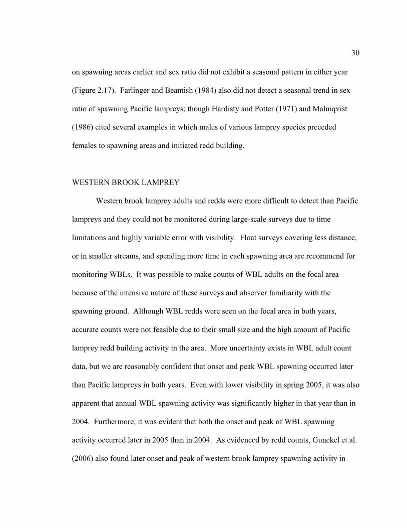
30
on spawning areas earlier and sex ratio did not exhibit a seasonal pattern in either year
(Figure 2.17). Farlinger and Beamish (1984) also did not detect a seasonal trend in sex
ratio of spawning Pacific lampreys; though Hardisty and Potter (1971) and Malmqvist
(1986) cited several examples in which males of various lamprey species preceded
females to spawning areas and initiated redd building.
WESTERN BROOK LAMPREY
Western brook lamprey adults and redds were more difficult to detect than Pacific
lampreys and they could not be monitored during large-scale surveys due to time
limitations and highly variable error with visibility. Float surveys covering less distance,
or in smaller streams, and spending more time in each spawning area are recommend for
monitoring WBLs. It was possible to make counts of WBL adults on the focal area
because of the intensive nature of these surveys and observer familiarity with the
spawning ground. Although WBL redds were seen on the focal area in both years,
accurate counts were not feasible due to their small size and the high amount of Pacific
lamprey redd building activity in the area. More uncertainty exists in WBL adult count
data, but we are reasonably confident that onset and peak WBL spawning occurred later
than Pacific lampreys in both years. Even with lower visibility in spring 2005, it was also
apparent that annual WBL spawning activity was significantly higher in that year than in
2004. Furthermore, it was evident that both the onset and peak of WBL spawning
activity occurred later in 2005 than in 2004. As evidenced by redd counts, Gunckel et al.
(2006) also found later onset and peak of western brook lamprey spawning activity in

31
2005 on the Smith River. However, in contrast to the South Fork Coquille, they observed
about 20% fewer WBL redds in 2005 than in 2004.
During both years of observation in the focal area and large-scale surveys, we
observed considerably more Pacific lamprey spawning activity than western brook
lamprey activity. While it was clear that the two species overlapped in spawning habitat
and range in the section of the South Fork Coquille River surveyed, it expected that the
western brook lampreys increase in relative abundance further upstream and in smaller
order tributaries. Such a species distribution pattern has been reported by both Luzier
and Silver (2005) and Gunckel et al. (2006).
CONCLUSIONS
This work evaluated spatial and temporal considerations for Pacific lamprey adult
and redd surveys. In addition, spawning time, length frequency, sex ratio, and movement
were described in a Southwestern Oregon coastal river system. Use of pontoon boats to
monitor spawners and their redds was a suitable approach for describing seasonal patterns
of relative spawning abundance. However, because spawner residence time appeared to
be less than one week, sample frequency needs to be almost daily to estimate absolute
population size. When adult densities were relatively high, seasonal patterns in spawning
activity were highly correlated spatially; thus it may be possible to gain comparable
information on relative abundance by monitoring a single, high-use spawning area.
Annual population monitoring can also be combined with larval emergence data to
evaluate reproductive success (see Chapter 3). Additional work on spawning surveys
should: (1) better quantify survey error sources, as done by Dunham et al. (2005) on bull

32
trout—especially observer variability in redd counts, diel variations in spawning time,
and differences between streams varying in size and habitat; (2) describe adult residence
time, sex ratio, and temporal differences to determine appropriate survey frequency; (3)
describe the mean and variance in number of redds produced per adult; and (4) lead to a
sampling manual with standardized protocols for adult and redd surveys that provides
pros, cons, error sources, and analysis considerations for each.

33
TABLES
Table 2.1. Dates of large-scale adult and redd surveys in 2004 and 2005. 2004 2005
April 29 §April 21 *May 5–6 April 28
*May 13–14 May 5 *May 19 & 21 ┼May 14
May 27 May 25 June 2 June 1
June 10 June 15 ┼June 30
*Survey required more than one day to complete §Zero fish counted ┼Zero fish measured Table 2.2. Reach information for large-scale surveys, ordered from upstream to downstream (9.2 km total).
Reach Start Position End Position Distance (kilometers)
Whiskey 42 54’ 21” N 124 06’ 40” W
42 54' 49" N 124 06' 09" W 1.2
Rowland 42 54' 49" N 124 06' 09" W
42 55' 16" N 124 07' 12" W 2.5
Long Tom 42 55' 16" N 124 07' 12" W
42 56' 02" N 124 06' 05" W 2.4
Beaver 42 56' 02" N 124 06' 05" W
42 56' 17" N 124 06' 07" W 0.7
Yellow 42 56' 17" N 124 06' 07" W
42 56’ 57” N 124 05’ 58” W 2.4

34
Table 2.3. Abundance (N) and mean length of live and dead Pacific lampreys during 2004 and 2005 large-scale surveys; excluding live fish seen but not captured (54 in 2004 and 31 in 2005).
Category Sex 2004 2005 N Size (cm) SE N Size (cm) SE
All Both 819 48.0 0.147 154 46.9 0.394 Males 450 50.0 0.173 83 48.3 0.491 Females 345 45.4 0.175 71 45.2 0.574
Live Both 446 47.4 0.200 140 46.6 0.409 Males 217 49.6 0.276 75 48.4 0.527 Females 229 45.4 0.211 65 44.5 0.531
Dead Both 373 48.6 0.212 17 49.4 1.231 Males 233 50.4 0.209 9 48.1 1.396 Females 116 45.4 0.310 8 50.9 2.056 Unsexed 24 45.8 0.939 0
Table 2.4. Total number of live adult Pacific lampreys per reach and number per total kilometer surveyed for 2004 and 2005 large-scale surveys. Reaches are ordered from upstream to downstream.
Year Data Type Whiskey Rowland Long Tom Beaver Yellow Total
Adults/reach 108 126 114 23 75 446
2004
Adults/km 15.5 8.5 7.8 5.4 5.2 8.1
Adults/reach 15 34 58 5 28 140
2005
Adults/km 1.4 1.5 2.6 0.8 1.3 1.7
Table 2.5. Total number of Pacific lamprey redds per reach and number per total kilometer surveyed for 2004 and 2005 large-scale surveys. Reaches are ordered from upstream to downstream.
Year Data Type Whiskey Rowland Long Tom Beaver Yellow Total
Redds/reach 232 405 570 125 421 1759
2004
Redds/km 33.4 27.2 38.8 29.4 29.1
31.9
Redds/reach 171 295 404 70 229 1169
2005
Redds/km 16.4 13.2 18.4 11.0 10.5 14.1

35
Table 2.6. Matrix of r2 statistics and associated P-values for relationships between weekly adult Pacific lamprey counts in each of the large-scale survey reaches, the entire large-scales section, and the focal area (combined 2004 and 2005 data; N = 15 for all survey types). Survey reaches are ordered from upstream to downstream.
Weekly Adult Count
Result Focal Area Mean
Large-scale Total
Whiskey Reach
Rowland reach
Long Tom
Reach
Beaver Reach
Yellow Reach
r2 0.690 0.526 0.584 0.668 0.637 0.702 Focal area mean P-value 0.0001 0.0022 0.0009 0.0002 0.0004 0.0001
r2 0.690 0.903 0.919 0.874 0.776 0.868 Large-scale Total P-value 0.0001 <0.0001 <0.0001 <0.0001 <0.0001 <0.0001
r2 0.526 0.903 0.872 0.697 0.609 0.651 Whiskey Reach P-value 0.0022 <0.0001 <0.0001 0.0001 0.0006 0.0003
r2 0.584 0.919 0.872 0.659 0.863 0.708 Rowland Reach P-value 0.0009 <0.0001 <0.0001 0.0002 <0.0001 0.0001
r2 0.668 0.874 0.697 0.659 0.558 0.828 Long Tom Reach P-value 0.0002 <0.0001 0.0001 0.0002 0.0014 <0.0001
r2 0.637 0.776 0.609 0.863 0.558 0.683 Beaver Reach P-value 0.0004 <0.0001 0.0006 <0.0001 0.0014 0.0001
r2 0.702 0.868 0.651 0.708 0.828 0.683 Yellow Reach P-value 0.0001 <0.0001 0.0003 0.0001 <0.0001 0.0001
Table 2.7. Number and mean lengths (cm) of tagged Pacific lampreys recaptured or recovered dead from large-scale surveys in 2004.
Category Sex Number recaptured Mean length
All Both 46 49.9
Live Both 11 49.8
Males 10 50.5
Females 1 42.5
Dead Both 35 49.9
Males 27 50.8
Females 8 46.9

36
Table 2.8. Tagging and recovery locations and weeks, and movement distance and direction for live Pacific lampreys recaptured during 2004 large-scale surveys.
Sex Reach Tagged Reach Found Direction Moved
Reaches Moved
Week Tagged
Week Found
M Yellow Long Tom upstream 2 1 2
M Yellow Whiskey upstream 4 2 3
M Yellow Rowland upstream 3 2 3
M Whiskey Rowland downstream 1 2 3
M Long Tom Long Tom stayed 0 2 3
M Yellow Long Tom upstream 2 2 3
M Yellow Yellow stayed 0 2 3
M Yellow Yellow stayed 0 2 3
M Long Tom Long Tom stayed 0 3 4
M Whiskey Long Tom downstream 2 3 4
F Rowland Yellow downstream 3 2 2
Table 2.9. Numbers and percent of Pacific lampreys from each tagging date recaptured on spawning grounds alive after one week in 2004; note that a female recaptured after only one day is excluded. Zero fish were recaptured in 2005.
Date Tagged Number Tagged Number recaptured alive Percent recaptured
29-Apr 25 1 4.00
5-May 155 7 4.52
13-May 169 2 1.18
19-May 92 0 0.00
27-May 1 0 0.00
2-Jun 4 0 0.00
Total 446 10 2.24
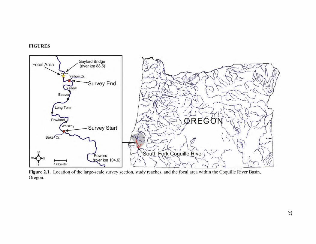
37
FIGURES
Figure 2.1. Location of the large-scale survey section, study reaches, and the focal area within the Coquille River Basin, Oregon.

38
Figure 2.2. 2004 and 2005 discharge (cubic feet per second) on South Fork Coquille River from January 1 to July 30.
Figure 2.3. Daily mean water temperature at the focal area from April 4 until August 3, 2004 and 2005.

39
0
20
40
60
80
100
120
140
160
180
29-Apr-04 6-May-04 13-May-04 20-May-04 27-May-04 3-Jun-04
Num
ber o
f adu
lt P
acifi
c la
mpr
eys
FM
N=446
Figure 2.4. Number of live adult male and female Pacific lampreys observed on spawning areas during 2004 large-scale surveys (all reaches combined).
0
10
20
30
40
50
60
21-Apr-05 5-May-05 19-May-05 2-Jun-05 16-Jun-05 30-Jun-05
Num
ber o
f adu
lt P
acifi
c la
mpr
eys
FMUK
*
N=140
Figure 2.5. Number of live adult male and female Pacific lampreys observed on spawning areas during 2005 large-scale surveys (all reaches combined). The star represents a survey in which zero fish were seen. Note difference in scale of y-axis between Figures 2.4 and 2.5.

40
Figure 2.6. Number of carcasses recovered in large-scale reaches during 2004 surveys. Reaches are ordered from upstream (Whiskey) to downstream (Yellow).
Figure 2.7. Number of carcasses recovered in large-scale reaches during 2005 surveys. Reaches are ordered from upstream (Whiskey) to downstream (Yellow).

41
87
791
610
189
73
90
100
200
300
400
500
600
700
800
900
29-Apr-04 6-May-04 13-May-04 20-May-04 27-May-04 3-Jun-04
Num
ber o
f red
ds c
ount
ed
N = 1759
Figure 2.8. Number of Pacific lamprey redds counted during 2004 large-scale surveys (all reaches combined).
5
83
299
16
227
384
123
14 180
50
100
150
200
250
300
350
400
21-Apr-05 5-May-05 19-May-05 2-Jun-05 16-Jun-05 30-Jun-05
Num
ber o
f red
ds c
ount
ed N = 1169
Figure 2.9. Number of Pacific lamprey redds counted during 2005 large-scale surveys (all reaches combined).

42
Figure 2.10. Number of redds counted versus number of live adult Pacific lampreys captured during weekly large-scale surveys.
Figure 2.11. Number of redds counted per adult versus days from the first adult was observed in large-scale surveys. A 5/27/04 observation of one fish and 73 redds, 28 days from the first adult observation, was omitted.
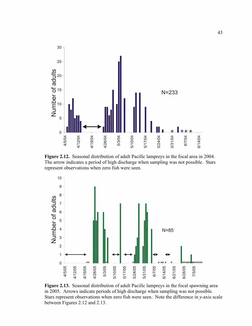
43
Figure 2.12. Seasonal distribution of adult Pacific lampreys in the focal area in 2004. The arrow indicates a period of high discharge when sampling was not possible. Stars represent observations when zero fish were seen.
Figure 2.13. Seasonal distribution of adult Pacific lampreys in the focal spawning area in 2005. Arrows indicate periods of high discharge when sampling was not possible. Stars represent observations when zero fish were seen. Note the difference in y-axis scale between Figures 2.12 and 2.13.

44
Figure 2.14. Weekly mean focal adult counts (fish per observation) versus number of live adult Pacific lampreys captured during weekly large-scale surveys.
Figure 2.15. Length frequencies of all male and female mature adult Pacific lampreys sampled in 2004 and 2005 (live fish and carcasses included).

45
Figure 2.16. Mean lengths of live mature adult Pacific lampreys collected from spawning areas on large-scale survey dates when fish were measured in 2004 and 2005. No males were measured on May 27, 2004 and no females were measured on June 15, 2005. Bars represent Bonferroni intervals from multiple comparison procedures. There were no statistically significant differences in length between any of the spawning groups in either year, except for females between April 28 and May 25, 2005.
Figure 2.17. Sex ratio of live adult Pacific lampreys on spawning grounds versus days since the first mature adult was observed in 2004 and 2005 large-scale surveys.

46
Figure 2.18. Number of mature western brook lampreys observed in the focal area in 2004 and 2005. Zeros denote observations in which no fish were counted.

47
CHAPTER 3
ANNUAL AND INTRA-ANNUAL PATTERNS IN PACIFIC LAMPREY SPAWNING, LARVAL RECRUITMENT, AND EARLY LIFE SURVIVAL IN A COASTAL
OREGON STREAM
INTRODUCTION
Egg and larval survival in riverine fishes tends to be low and unpredictable
compared to other life stages (Houde 1987; Kempinger 1988; Magnuson 1991;
Bjorkstedt 2000; Pepin 2002). For this reason, differences in mortality during these
stages can have important consequences for year-class success and eventual adult
recruitment (Hjort 1914; Rice et al. 1987; Elliot 1989; Leggett and DeBlois 1994;
Johnston et al. 1995; Houde 2002). Spawning stock size or total egg production sets the
upper potential for larval recruitment, but realized recruitment is lowered due to limiting
biotic and abiotic factors occurring during development (Corbett and Powles 1986; Elliot
1989; Leggett and DeBlois 1994; Houde 2002). Clarifying the relationship between
spawning stock size and larval recruitment and identifying mechanisms underlying
variability in early life survival are essential steps in modeling fish populations and
implementing successful monitoring and recovery plans.
Despite its recognized importance in fish population dynamics, the period from
spawning until larval emergence remains the least understood part of many species’ life
cycles. The Pacific lamprey, Lampetra tridentata, is no exception. Excluding a
laboratory study investigating the effects of temperature on developing embryos
(Meeuwig et al. 2005), research has focused on adults and older size-classes of larvae,
while neglecting the critical incubation period. Therefore, the overall goal of this study

48
was to describe patterns of Pacific lamprey larval recruitment and early life survival in
the wild.
An extremely fecund species, Pacific lampreys lay between 98,000 and 240,000
eggs (Kan 1975); though, only a minute fraction are expected to survive to maturity. For
the Great Lakes sea lamprey, Petromyzon marinus, only 14% of a female’s eggs were
estimated to reach the redd gravels, but up to 90% of these survived until hatching (13–15
days; Manion and Hanson 1980). Manion (1968) estimated that, on average, only 6.3%
of a female’s eggs survive until hatching. Comparatively low densities of age-0 lampreys
in rearing habitats additionally indicate that only a small percentage of individuals
survive until the larval, or ammocoete, stage (Jones and Derosier 2002; Torgersen and
Close 2004). Mortality of ammocoetes in the substrate, however, is thought to be
relatively low, declining with increasing size (Pletcher 1963, Manion 1968; Hardisty and
Potter 1971a; Potter 1980). As a result, survival between time of spawning and
ammocoete settlement into rearing substrates is hypothesized to be central in determining
outmigrant production (see Chapter 1 for a full life history description).
Among the most important factors that influence survival and recruitment during
early life stages are spawning time, density of spawning adults, discharge, water
temperature, and predation. There is strong selective pressure for linking timing of
spawning and emergence with ecological conditions favorable for early-life survival
(Flecker 1992; Frank and Leggett 1994; Dahl et al. 2004). In most temperate river
systems, environmental stochasticity is the norm, and many fish species have evolved to
spawn over a prolonged period as a way of hedging their bets against such variation
(Quinn and Adams 1996; Humphries et al. 1999). Pacific lampreys spawn over a period

49
of 3–4 months (Kan 1975; Richards 1980; current study) and offspring of earlier
spawning individuals can be exposed to a suite of environmental conditions that differ
markedly from those experienced by offspring of later spawning individuals. For this
reason substantial seasonal and annual differences in spawning time and egg and larval
survival are expected.
Understanding the relationship between spawning stock and larval recruitment is
essential for evaluating early life survival, yet the stock-recruit relationship has not been
described for the Pacific lamprey. In highly fecund fishes, there is typically a non-linear
relationship between the number of spawning adults and the number of young produced
(Hjort 1914; Houde 1987; Bjorkstedt 2000). Investigations into sea lamprey population
dynamic, for example, show a high amount of density-independent variation in
recruitment to age-1, but a general reduction in recruitment at highest spawner densities
(Jones et al. 2003; Haesker et al. 2003). Because lampreys spawn in limited benthic
habitats, density dependent mechanisms may influence their survival and recruitment.
Lowered recruitment of lotic fishes at higher spawner densities can result from redd
superimposition by later spawning adults (Manion and Hanson 1980; Van den Berghe
1989; Fukushima et al. 1998; Jones et al. 2003), and intraspecific competition for limited
food or habitat resources during juvenile stages (Elliot 1989; Weise and Pajos 1998;
Partridge and DeVries 1999).
Discharge during spawning and development has also been shown to influence
early life survival of lotic fish (Kempinger 1988; Scrivener et al. 1989; Johnston 1995;
Fukushima et al. 1998; Mion 1998), but the effects of discharge on Pacific lamprey are
unknown. We hypothesized that high flow events, which are common in Northwest

50
coastal rivers during the lamprey spawning season, would result in lowered cohort
survival due to decreased egg deposition, scouring of eggs and prolarvae from redd
gravels, and desiccation of redds associated with rapidly dropping river levels following
these events.
As with other fishes (Alderdice and Velsen 1978; Hamel et al. 1997; Benoît and
Pepin 1999; Pitlo 2002), water temperature is also a crucial parameter in development
and survival of lamprey embryos (Pletcher 1963; Rodríguez-Muñoz et al. 2001; Meeuwig
et al. 2005). In a laboratory setting, Meeuwig et al. (2005) found a sharp decline in
survival of both “fertilization-to-hatch” and “hatch-to-larvae” stages as rearing
temperature increased from 18ºC to 22ºC. Embryos reared at 22ºC were also shown to be
approximately six times more likely to have developmental abnormalities than those
reared at lower temperatures (Meeuwig et al. 2005). The impact of water temperature on
Pacific lamprey reproductive success has also not been evaluated in the wild and may
differ from laboratory studies because of fluctuating temperatures and ecological
interactions. Based on the results of Meeuwig et al. (2005) we anticipated that water
temperatures in excess of 18–22°C during spawning and egg development may reduce
larval survival.
Predation is a final source of early life mortality thought to be important in Pacific
lamprey early life survival and recruitment. Numerous fishes, including rainbow trout,
sculpin, stickleback, and dace have been observed feeding on eggs in lamprey redds
during and after spawning (Pletcher 1963; Manion 1968; Hardisty and Potter 1971a).
Preliminary observations from our study site indicated high densities of speckled dace
(Rhinichthys osculus) in and around Pacific lamprey redds during and after spawning.

51
For this reason, we hypothesized that egg predation could be a significant factor in
lamprey spawning success. Although it is clear that fish readily consume lamprey eggs,
the recruitment consequences of this predation are unknown.
A challenge in studies of early life mortality and larval recruitment involves
selecting an appropriate time scale for observation. Ecological conditions occurring
before, during, and after spawning can influence reproductive success and should be
considered when investigating recruitment processes (Rice et al. 1987; Kempinger 1988;
Houde 2002; Pitlo 2002). This within-season variability is often overlooked when
evaluating recruitment on an annual basis. An alternative to annual assessment of fish
populations is analysis of intra-annual cohorts in relation to environmental variation
occurring within spawning and development seasons (Rice et al. 1987; Elliot 1989; Mion
1998; Partridge and DeVries 1999; Hoffman and Olney 2005). Such an approach may
help reveal mechanisms underlying variability in year class strength.
In this study we examined intra-annual cohorts of Pacific lamprey spawning
adults and their larvae during 2004 and 2005 on the South Fork Coquille River to address
the following questions: 1) How does spawning time and ammocoete production vary
between and within years and in relation to environmental conditions? 2) What is the
relationship between spawning stock and larval recruitment? And 3) how are spawning
stock, temperature, discharge, and egg predation related to cohort survival until larval
emergence?

52
METHODS
SAMPLING SITE
The primary sampling site, designated the focal area, encompassed a single
Pacific lamprey spawning area (ca. 30x30m) and a riffle-pool sequence immediately
downstream. The focal area was located about 200 m upstream of Gaylord, OR (42 57’
22” N, 124 06’ 21” W) at river kilometer 88.6, and was selected based on its reputation
for being a heavily used spawning area and for ease of nighttime access (Figure 3.1). The
closest Pacific lamprey spawning area was approximately 300 m upstream, immediately
below which was a long pool with substantial depositional habitat.
ABIOTIC VARIABLES
Water temperature was monitored at 30 minute intervals from April 27–July 13,
2004 and from April 4–August 3, 2005 using an Onset Optic Stowaway Temp Logger®
placed in a shaded area at the river bottom directly downstream of the focal area. From
April 6–April 27, 2004 water temperature was recorded daily with a bulb thermometer
and daily mean temperatures were estimated based on bulb temperature at time of
observation in relation to diel temperature trends in early May, 2004. Daily mean water
temperature during periods before April 6 in 2004 and April 4 in 2005 were predicted
using year-specific multiple linear regression models with maximum daily air
temperature at Powers and loge of discharge as explanatory variables (2004, R2 = 0.863, P
< 0.0001; 2005, R2 = 0.918, P < 0.0001).
On-site discharge data were obtained from a U.S. Geological Survey (USGS)
gauging station located at Powers, OR, 14.5 river km upstream of the focal area

53
(“POWO3”; 42 53'31" N, 124 4'16" W). No significant tributaries enter the river section
between the gauge and the focal area. Lunar phase and fraction of moon illuminated,
defined as illuminated area of the moon’s apparent disk divided by total disk area, were
obtained from the US Naval Observatory web page
(http://aa.usno.navy.mil/data/docs/moonphase.html).
SPAWNING ACTIVITY
Pacific lamprey spawning activity in the focal area was monitored in 2004 and
2005 using counts of mature adults as an index of spawning activity. Counts were
obtained by systematically wading through the focal area on 38 days between March 28
and July 12, in 2004, and on 46 days from April 5 until July 17, in 2005. When visibility
permitted, counts were made in late afternoon and separated by no more than 4 days
during the spawning season.
LARVAL PRODUCTION
Abundance of age-0 ammocoetes was monitored every three or four days
(biweekly samples) from April 11 to July 14, 2004 and April 25 to July 28, 2005 at a site
on the downstream margin of the focal area. Emergent ammocoetes from these samples
were used as surrogates for intra-annual cohorts. Beginning and ending sampling dates
encompassed the period of larval emergence predicted from observed spawning times,
estimated incubation time, and water temperature. Drift sampling ceased after no
emergent ammocoetes were caught for 4–5 consecutive samples. Biweekly samples were
collected using a 500 µm mesh zooplankton-drift net [0.70 x 1.5 m opening; 2.5 m long;

54
“large net”] fastened to steel posts driven into the substrate, 27 m downstream of the
focal area boundary. Each sample was collected between 2 and 3 hours after civil
twilight (time sun is 6º below horizon; U.S. Naval Observatory web page:
(http://aa.usno.navy.mil/) in 2004 and approximately 3 hours after civil twilight in 2005.
Net position relative to stream width was within 2 m of the thalweg (6–12 m from the
stream margin) except during periods of high water when the net had to be set closer to
the stream margin. With few exceptions, the net covered the entire water column depth.
Depending on flow conditions and concentrations of net-clogging detrital matter, each net
was fished for 7–16 minutes. A TSK mechanical flowmeter was centrally mounted in the
net opening to estimate water velocity and volume filtered. Variation in net efficiency
across sample dates due to clogging was assumed negligible for age-0 ammocoetes
because of their poor swimming ability. High river levels limited access to the net-site on
two dates in 2004 and five in 2005 and an alternate site approximately 200 m upstream
had to be used. Of these alternate samples, only the last three in 2005 contained age-0
ammocoetes and were included in analyses of larval production from the focal area.
Net samples were rinsed into the cod-end using a battery powered wash-down
pump. Contents were treated with rose bengal bioactive staining agent to facilitate
sorting and preserved in 5% formalin. Age-0 ammocoetes were sorted and counted in the
laboratory under magnification and measured to the nearest 0.1 mm total length using a
dissecting scope equipped with an ocular micrometer. For samples containing more than
100 age-0 ammocoetes, a random subsample of 100 individuals was measured. Emergent
ammocoetes were defined as individuals >7.9 mm and < 9.1 mm (“8–9” mm). The
emergent size range was based on lengths from early season samples—when all

55
individuals were expected to be emergent—and lengths of larvae hatched in captivity (M.
Meeuwig, USGS, personal communication). A pilot project, in which eggs were reared
in situ until emergence, verified emergence in the 8–9 mm size range (see Appendix I).
We assumed that the emergent size range did not change across sampling dates and years.
Female size influences size of offspring (Elliott and Hurley 1998; Benoit and Pepin,
1999), but no temporal differences were detected in size of Pacific lamprey females in the
South Fork Coquille River (see Chapter 2).
Age-0 ammocoetes larger than 9.0 mm were assumed to represent upstream
production and not emergent larvae from the focal area. Larvae smaller than 8.0 mm
were excluded from analyses of Pacific lamprey larval production due to the possibility
they were western brook lampreys. Prior research indicates that both mean egg diameter
and emergent larval length of western brook lampreys are significantly smaller than those
of Pacific lampreys (Pletcher 1963; Meeuwig et al. 2004).
Seasonal comparisons of larval abundance were based on a standardized drift rate,
defined as individuals drifting past the wetted-width cross section per minute, which was
calculated as: individuals per m3 H2O * discharge (m3 H2O/second) * 60 seconds/minute.
This measure of larval abundance was selected to adjust for variable stream discharge
between samples. However, there was a strong correlation between drift rate (individuals
per minute) and drift density (individuals per m3 H2O) and similar results were obtained
using either measure (r2 = 0.963; P < 0.0001).
For calculations of drift rate, we assumed that density of drifting ammocoetes was
uniform across the stream during the sample period and tested this assumption using
smaller, paired drift nets (0.30 m x 0.45 m opening, 1 m long; 500 µm mesh; “small

56
nets”) set on either side of, equidistant from, and concurrent with biweekly nets. Each
pair of nets consisted of a top and bottom net stacked to cover the water column, the
contents of which were combined into a single net sample for analysis. Volume of water
filtered was estimated from area of the net opening, time fished, and water velocity,
which was measured using a pole-mounted TSK flowmeter held stationary in each net
center for 1 minute. These “spatial” samples were taken on three occasions in 2004.
Differences in age-0 ammocoete drift density between net positions across the wetted-
width were not significant (ANOVA: F2,6 = 0.02, P = 0.98). For seasonal comparisons of
larval production, we also assumed that the percentage of total drifting larvae caught at
the biweekly net position was consistent across sampling dates.
Drift samples were collected throughout 24-hour cycles to investigate diel
patterns in ammocoete drift behavior and assess whether biweekly samples collected 2
and 3 hours after sunset were representative of relative drift abundances on sample dates.
Diel samples were collected on 6–7 June and 28–29 June in 2004, and 13–14 June and 5–
6 July in 2005 using paired small nets stacked to cover the water column. In 2004,
samples were taken concurrently at the biweekly net-site, and a site immediately
upstream of the focal area, resulting in two diel cycle samples for each sample date. In
2004 samples were collected at 1–4 hour intervals at 0800, 1200, 1600, 2000, 2100, 2200,
2300, 0000, 0200, 0400, 0500, and 0600 hours. Nets were fished for 20 minutes during
daylight and 10 minutes during dusk, dawn, and darkness. In 2005 paired diel nets were
set at the biweekly net site for 15 minutes, at 2100, 2200, 2300, 0000, 0200, 0400, 0500,
and 0600 hours. No daylight samples were taken in 2005 because 2004 diel samples
verified that ammocoetes seldom move during these times. Volume of water filtered was

57
estimated as described above. Because river discharge was essentially constant during
24-hour sample cycles, results were expressed as standardized drift densities (individuals
per m3 H2O filtered). Drift densities from each net were normalized by expressing them
as a percent of the total density captured during a 24-hr sample cycle. Over the six diel
sampling events, hourly differences in percent of total daily drift density were compared
using One-way ANOVA. Bonferroni's multiple comparison procedure was employed to
determine significance among sample times.
EGG PREDATION
Speckled dace and other likely egg predators were surveyed qualitatively in the
focal area by sight, under water photography, and video and categorized into the
following feeding activity levels: Level 1, a non-feeding observation, when speckled
dace were absent or scattered and in low densities relative to lamprey redds; Level 2,
when dace were aggregated in and behind spawning lampreys or active redds in
comparatively high densities, but not seen feeding aggressively; and Level 3, feeding-
frenzy, when high densities of dace (~100 per m3) were congregated in or behind recently
spawned-in redds and actively feeding on eggs.
To verify that speckled dace were indeed consuming lamprey eggs, a small
number were collected during apparent feeding events, anesthetized, and preserved in
10% formalin for inspection of stomach contents. Stomach contents were dissected from
individual dace and examined under a dissecting microscope. Probable Pacific lamprey
eggs were compared to a sample of fertile eggs obtained from a manually spawned pair
(Appendix I).
58
DATA ANALYSES
Linking Larval Drift Samples with Corresponding Adult Counts
Spawning dates for emergent ammocoete cohorts were estimated by
backcalculating from the capture date to the date required to achieve 300.7 effective
degree-days (EDD). This EDD estimate was based on temperature units required to
reach larval stage 18 (Piavis 1961), which was calculated from a USGS laboratory study
on Pacific lamprey eggs reared at constant water temperatures of 10, 14, 18, and 22ºC
(Meeuwig et al. 2005; Table 3.1). Effective degrees for each day were calculated by
subtracting the theoretical temperature for zero development, 4.85ºC (Meeuwig et al.
2005), from the daily mean water temperature. The predicted spawning date for each
emergence date was the date at which cumulative EDD was closest to 300.7 (Table 3.1).
Duration of embryonic development was the number of days between emergence and the
estimated spawning date. The predicted spawning period for each larval cohort was the
period corresponding to the day before a larval drift sample to the day after a larval drift
sample, which ranged from 2–5 days. The sum of adult counts during this period was
used as an estimate of spawning stock in analyses.
Because adult counts were not available for all days in spawning periods
corresponding to each emergence date, we generated estimates of adult counts for all
missing days (Appendices IV, V). Based on previous research (Pletcher 1963; Kan 1975;
Close et al. 2003) and observations from the current study, adult spawning activity was
assumed to be zero on days with daily mean water temperature below 11ºC. Missing
adult counts were estimated from simple linear regressions of actual counts on daily
mean water temperature from April 6–May 19 in 2004 (r2 = 0.356, P = 0.0034) and April

59
5–June 5 in 2005 (r2 = 0. 217; P = 0.0287). Temperature-predicted regression estimates
for missing dates were then adjusted based on the residuals of actual adult counts on the
two adjacent dates. The residuals were weighted based on proximity of actual counts to
the missing dates, and t he sum of the two weighted residuals were added to the
regression estimate for the missing date. For example, if actual adult counts on May 9
and May 11, were 10 and 20, but temperature-predicted regression estimates were 12 and
14, respectively, then the regression estimate for May 10 would be adjusted by +2, or
50% of the residual from May 9 (-1) plus 50% of the residual from May 11 (+3).
Spawning activity after May 19 in 2004 and June 5 in 2005 were not described by linear
temperature models; therefore adult estimates were generated using simple linear
interpolation between actual adjacent adult counts.
In analyses of stock-recruitment and survival until emergence, we only included
data points in which both emergent larvae and corresponding spawners were present
(N=26). These points consisted of all larval drift samples from May 13–June 24, 2004
(N=13) and May 30–July 14, 2005 (N=13), which constituted 99.8% and 97% of
seasonal larval production, respectively. Of these 26 spawning periods, only two
spawning stock estimates, both in 2005, were comprised entirely of predicted adult
counts.
There are a number of error sources to consider when linking intra-annual larval
cohorts with spawning adults. First, duration of the incubation period until emergence
can differ between laboratory-reared eggs and those reared in situ. In this case, days
from fertilization to larval emergence in the wild may not be equivalent to days from
fertilization to larval stage 18 in the lab (burrowing stage; Piavis 1961; Meeuwig et al.

60
2005), which was used as proxy for emergence. Designation of stage 18 involves
inspection of level of yolk extrusion from the gut and is a rather qualitative assignment
(M. Meeuwig, USGS, personal communication). Furthermore, naturally fluctuating
temperature regimes in the field can lead to different development rates than eggs reared
at constant temperatures in controlled laboratory studies (Alderdice and Velsen 1978;
Hamel et al. 1997). Derosier (2001) found that it took 8.6% and 38.6% more cumulative
degree days for 50% larval emergence to occur for sea lampreys in two Lake Huron
tributaries, than for 50% of individuals reared at constant temperature in laboratory
experiments to reach the burrowing stage (Stage 18; Piavis 1961). On the contrary,
Bestgen and Williams (1994) found little difference in time of hatch between fluctuating
and constant temperatures over a range of mean development temperatures for Colorado
pikeminnow, Ptychocheilus lucius. Notably, light intensity (John and Hasler 1956),
oxygen concentration (Shumway et al. 1964; Hamor and Garside 1976), and photoperiod
(Hamel et al. 1997) have also been shown to influence fish development rate and each of
these factors could change over time and differ between field and laboratory settings.
A second potential error source in linking larvae with their parents involves
variation in time of larval emergence from a single redd. Our in situ incubation pilot
project showed that larvae from eggs fertilized on the same date emerged over a period of
nearly two weeks, with 70% emerging over a 5-day period (Appendix I). This result
suggests that either, there was substantial variation in development rate, or larval
emergence timing was controlled in part by factors other than developmental stage.
Derosier (2001) concluded that sea lamprey larvae from like-nests emerged over a period

61
of 3–14 days; although her sampling design almost certainly caught larvae originating
from multiple nests.
Third, multiple methods can be used to predict spawning time based on water
temperature, and error is introduced from the temperature-development model selected
(Hamel et al. 1997). We used a cumulative effective degree-day model to match intra-
annual cohorts of drifting larvae with corresponding spawning periods. The degree-day
model is relatively simple and assumes a linear increase in developmental rate with
temperature. Although it has been criticized for its lack of application outside a central
range of temperatures (Alderdice and Velsen 1978), Hamel et al. (1997) showed that, for
white sucker, Catostomus commersoni, the degree-day model was at least as accurate as
several more complex models. At the moderate range of temperatures experienced by
most developing embryos in this study, it is safe to assume that the degree-day model was
reasonably accurate in its prediction of incubation time (Hamel et al. 1997). Using this
model, the last newly-emerged larvae collected in both years were within 3–4 days of
dates predicted from water temperature and adult observations. Moreover, 50% of larvae
reared in the in situ egg incubator, at a mean temperature of approximately 15°C,
emerged within 3–4 days of the time predicted using the degree day model (Appendix I).
In spite of the potential drawbacks of using a temperature-development equation
obtained from laboratory data, our results suggest the methods employed were adequate
to predict spawning time at the temporal resolutions considered. If consistent across
temperatures, these error sources are unlikely to alter our conclusions about relative
survival and stock-recruitment.

62
The relationship between adult counts and actual spawning can also be questioned
as a potential bias when linking intra-annual larval cohorts with their parents. Even
though the majority of fish observed in the focal area were not in the act of spawning, we
believe presence of adults was an accurate surrogate for spawning activity. First, nearly
all of adult Pacific lampreys observed were either in the process of redd-digging or were
resting in the vicinity of a redd. Secondly, all adults examined exhibited characteristics
of ripe fish: enlarged dorsal and caudal fins, engorged false anal fins in females, or
running ripe with eggs or milt. Finally, results from a tagging study (See Chapter 2)
suggest that the period of residence on spawning grounds is typically not more than one
week. Farlinger and Beamish (1984) also estimated that Pacific lampreys remain on
spawning grounds for about 5 days.
Stock – recruitment
The relationship between spawning stock and downstream larval recruitment was
evaluated using a simple linear regression model of loge of emergent larval recruitment
(drift rate) versus loge of spawning stock. A Ricker stock-recruitment model was fit to
the same data for comparative purposes using the following equation (Ricker 1975):
Equation 1: R = α*S*e-β*,
where R is larval recruitment, S is corresponding spawning stock, α is the coefficient of
density-independent mortality, and β is the coefficient of density-dependent mortality.
The parameters α and β were obtained from the exponentials of the intercept and the
slope, respectively, of a simple linear regression of loge larval recruitment per spawning
stock versus spawning stock.

63
Survival until Larval Emergence
Relative Pacific lamprey reproductive success, or survival until larval emergence,
was assessed by comparing larval production per spawning adult between and within
2004 and 2005 spawning seasons. Annual survival was contrasted using a “Relative
Survival Index,” calculated by dividing total annual drift rate of emergent larvae by the
estimated annual number of spawners. Monthly indices of survival until emergence were
calculated for each spawning month, by dividing the percent of total annual emergent
larval production by the percent of annual spawners in that month. Survival until
emergence was assessed for each intra-annual cohort as emergent larval production per
spawner. We assumed that average fecundity, which is related to female length
(Malmqvist 1986), was unchanged throughout the spawning season since there were no
significant differences in mature female lengths between sampling dates (see Chapter 2).
Explaining Survival until Larval Emergence
Simple linear regression was employed to examine relationships between cohort
survival until emergence and the following variables: mean water temperature during the
development period (MWTD), number of days daily mean water temperature exceeded
20°C during development (DMWT20+), mean water temperature during the spawning
period (MWTS), stream discharge during each drift sample (discharge), mean discharge
during the development period (MDD), number of days daily mean discharge exceeded
1000 cfs during development (DMD1000+), mean discharge during the spawning period
(MDS), fraction of the moon illuminated during each drift sample (FMI), number of adult
Pacific lamprey present during each corresponding spawning period (SS), duration of the

64
development period (DDP), and Year (Table 3.2). Where necessary, data were loge
transformed before regression to meet conditions of normality and constant variance, or
to improve linearity. Conditions occurring during periods of high and low survival were
also evaluated using two sample t-tests to compare mean values of each explanatory
variable between cohorts with the highest 50% of survival values, and those with the
lowest 50% of survival values.
After evaluating univariate relationships, a list of prospective multiple linear
regression models was selected from a subset of predictor variables (Table 3.2) and
narrowed-down using the information-theoretic approach (Burnham and Anderson 1998).
Initially the “regression selection” feature of STATGRAPHICS was employed to fit all
possible one to five variable combinations of nine potential explanatory variables,
including an interaction term between SS and MDS, and an indicator variable for Year
(Table 3.2). This procedure resulted in a preliminary list of 382 models. A matrix of
correlations was used to identify high correlation between independent variables
(Appendix VI). Models having highly correlated variables were inspected for serious
multicolinearity by calculating Variance Inflation Factors (VIF) of their parameters using
STATGRAPHICS. Only models containing parameters with VIFs less than 5 were
retained. Additionally, models containing the interaction term but not both interacting
variables were eliminated, resulting in 145 candidate models.
Akaike Information Criterion (AIC) values with a small sample size correction
(AICc; Hurvich and Tsai 1989) were calculated for the 145 remaining models using
Equation 2 (Burnham and Anderson 1998; p. 51) and subsequently arranged in ascending
order of AICc value.

65
The first term in Equation 2 measures goodness of fit of the model, and the second term
represents a penalty for increasing numbers of parameters (Burnham and Anderson
1998). Log(L(θ)) represents the log-likelihood estimator, K represents the number of
parameters in the model, and n equals sample-size. The log-likelihood estimator was
approximated as log(L(θ)) = -½n log(σ̂ 2) (Burnham and Anderson 1998; p. 17). The
multiplication of the term 2K by n/n-K-1, a small sample size correction factor, is
recommended when the ratio of n–K is less than 40 (Burnham and Anderson 1998).
Models with smaller AICc values provide a more parsimonious explanation of variation
in the dependent variable than models with larger values (Burnham and Anderson 1998).
ΔAICc, or the difference in AICc values between each model and the model with
the smallest AICc value (“top model”), were calculated to assist in model evaluation.
Models with ΔAICc values ≤ 2.0 were considered competing with the top model
(Burnham and Anderson 1998) and received consideration in the discussion. Akaike
weights (w) were also calculated for each model to aid in their comparison using
Equation 3 below (Burnham and Anderson 1998; p. 124).
ΔAICci equals AICc for the ith model minus the AICc value for the top model. Finally,
relative importance values for each explanatory variable were then computed from the

66
145 candidate models by summing wi for all models in which a given variable appeared.
Importance values offer a means of evaluating each explanatory variable’s relative
weight in explaining the variability in the response.
Lastly, a stepwise linear regression model selection technique was employed with
the same explanatory variables using Splus (Table 3.2). This technique consisted of
alternating forward selection and backward elimination steps until no explanatory
variables could be added or removed. Stepwise regression acted as a separate means for
selecting a suitable model from the pool of available explanatory variables (Table 3.2), as
well as a substantiation of variables selected using AICc.
Dace activity level during spawning was excluded from regression models due to
a small sample size in periods corresponding to intra-annual cohort spawning periods (N
= 16). Instead, differences in mean lamprey survival until emergence at each dace
feeding level were examined using a one-way ANOVA. To better understand observed
patterns of dace activity, factors hypothesized to influence dace feeding level, such as
water temperature and density of spawning Pacific lampreys, were also investigated using
one-way ANOVA.
RESULTS
ABIOTIC VARIABLES
Discharge during the 2004 lamprey spawning season was marked by a single,
mid-April high-flow event, which peaked on April 21 at 4840 cfs (Figure 3.2). In 2005
three substantial high-flow events (> 2000 cfs) occurred early and two smaller events

67
(851 and 1030 cfs) occurred later in the spawning season (Figure 3.2). During the April–
July spawning periods stream discharge was inversely related to water temperature (2004
and 2005 combined; r2 = 0.865; P < 0.0001; Figures 3.2, 3.3). Average water
temperature from April 6–July 13 was about 15% higher in 2004 (16.3ºC) than in 2005
(14.0ºC). In both years, water temperature rose gradually during spring, but diel
fluctuations of up to 8ºC occurred (Figure 3.3). Full moons occurred near the beginning
of each month in 2004 and towards the end of each month in 2005.
SPAWNING ACTIVITY
In 2004, 233 adult Pacific lampreys were counted in the focal spawning area
between April 6 and June 3 (Figure 3.4), with 95% observed by May 17. The maximum
number counted per day was 27, on May 4 (Figure 3.4), and mean number per day during
the spawning period was 8.32±1.24 (mean±SE). A large spring freshet in mid–late April
precluded observations (Figures 3.2, 3.4).
In 2005, 85 fish were counted in the focal area, with a mean of 2.65±0.50 fish per
survey during the spawning period. Spawning began later and occurred over a more
prolonged period than in 2004, from April 25 through July 3, with 95% of observations
occurring by June 6 (Figure 3.5). In spawning activity was bimodal, with peaks in late
April and from late May to early June (Figure 3.5). The maximum number counted per
day was nine, on April 26 (Figure 3.5). The five moderate to high flow events in 2005
precluded adult observations (Figures 3.2, 3.5).
Mean water temperature during both spawning seasons was approximately 15ºC,
with mature adults observed at a daily mean temperature ranged from 11.1–19.7 ºC

68
(Figure 3.6). Spawning activity generally exhibited a curvilinear relationship with water
temperature. In both years, the number of adults observed peaked between 13°C and 16
ºC, declining at temperatures above and below this range (Figure 3.6). Mature adults
were observed at the focal area at daily mean discharges of 124–932 cfs, with maximum
spawning activity occurring from around 200–500 cfs (Figure 3.7).
Water temperature during spawning was highly correlated with both mean
temperature (r2 = 0.768; P < 0.0001) and discharge (r2 = 0.615; P < 0.0001) during egg
and larval development. In contrast, discharge during spawning was only moderately
related to mean water temperature (r2 = 0.283; P = 0.0017) and discharge (r2 = 0.274; P =
0.0021) during development.
LARVAL PRODUCTION
In 2004, 74 drift samples (26 biweekly and 48 diel) were taken between April 11
and July 14 (Table 3.3). A total of 6901 age-0 ammocoetes were captured in the 26
biweekly samples. Fifty-five percent of these individuals were newly-emerged (8–9 mm
size-class), 43% were greater than 9 mm, and 2% were less than 8 mm. Early season
biweekly nets in 2004 caught predominately 8–9 mm individuals, with the proportion of
older and larger age-0 larvae increasing as the season progressed (Figure 3.8).
Emergent ammocoetes occurred in the drift for a 54 day period in 2004, from May 6 until
June 28—30 days after the first, and 25 days after the last adult was detected in the focal
area (Figures 3.4, 3.8). Emergent ammocoete abundance averaged 353.3±141.6
(mean±SE) fish per minute, peaking in mid-May at 2131.9 fish per minute.
Approximately 60% of emergent ammocoetes were captured by May 24, and 99% by

69
June 21. The median emergence date, when 50% of the annual abundance was captured,
occurred between May 20 and 24.
During the emergence period in 2004 (May 6 – June 28), abundance of emergent
ammocoetes was significantly correlated with abundance of age-0 ammocoetes larger
than 9 mm (r2 = 0.501; P = 0.0022; loge-loge model). Abundance of larger (>9 mm)
ammocoetes peaked at 610.2 per minute in early June, and remained high throughout the
month (Figure 3.8). A low number of larvae <8 mm, likely western brook lampreys,
were caught between May 27 and June 21, peaking on June 10 at 57.1 fish per minute
(Figure 3.8).
In 2005, 43 drift samples (27 biweekly and 16 diel), were collected between April
25 and July 28 (Table 3.3; Figure 3.8). A total of 2,854 age-0 ammocoetes were
collected in biweekly samples, of which approximately 48% were newly-emerged, 50%
were greater than 9 mm, and 2% were less than 8 mm. Emergent ammocoete drift rate
during 2005 was about a third lower than in 2004, with a mean of 112.1±34.9 individuals
per minute. Emergent ammocoetes were present in the drift over 71 days in 2005—from
May 15, 20 days after initial adult detection, to July 25, 22 days after final adult detection
(Figures 3.5, 3.8). Emergent ammocoete drift rate exhibited two distinct peaks in 2005;
the first and largest (550.9 fish per minute) around mid-June, and the second (405.2 fish
per minute) in early July (Figure 3.8). Approximately 60% of emergent ammocoete
production occurred by June 18, about half way thorough the observed emergence period.
The median emergence date occurred between June 12 and June 15 in 2005.
Unlike 2004, during the emergence period in 2005 (May 15 – July 25) abundance
of emergent ammocoetes was only weakly correlated with abundance of age-0

70
ammocoetes larger than 9 mm (r2 = 0.148; P = 0.0572; loge-loge model). Ammocoetes
>9 mm were captured in three main peaks in 2005: early, mid, and late June (Figure 3.8).
In contrast to 2004, a relatively high number of larger age-0 ammocoetes were present in
early season samples—sometimes in numbers greater than the emergent size-class
(Figure 3.8). A few smaller larvae (<8 mm) were caught between May 26 and July 17,
with drift rate peaking at 58.2 fish per minute on June 22.
Mean water temperature during development of larval cohorts ranged from
12.55°C to 18.26°C in 2004, and from 11.81°C to 21.85°C in 2005 (Figure 3.9).
Duration of the development period (DDP), or number of days between spawning date
and emergence date, which was estimated from effective degree-days, ranged from 21–42
d in 2004 and 18–49 d in 2005. In both years, peak larval production occurred at mean
development temperatures of approximately 13–16°C, with 69.2% of larvae developing
within that range (Figure 3.9). Above mean development temperatures of 16°C,
recruitment generally declined with increasing water temperature (Figure 3.9). Water
temperature during development increased seasonally, and later emerging larvae were
generally exposed to higher development temperatures than earlier larvae (Figure 3.10).
During development of larvae emerging after June 15, 2004 and June 29, 2005, daily
mean water temperatures commonly surpassed 20°C—the level predicted to be
detrimental to larval survival (Meeuwig et. al 2005; Figure 3.3).
Mean water temperature during development was inversely related to mean
discharge during development (r2 = 0.793; P < 0.0001). In both years, mean discharge
during development declined seasonally (Figure 3.10). Developing larvae were exposed
to mean discharges ranging from 152–685 cfs in 2004 and 71–841 cfs in 2005 (Figure

71
3.11). Larval production displayed a weak curvilinear relationship with mean
development discharge; generally increasing with discharge up to 600 cfs, and decreasing
with discharge above 600 cfs (Figure 3.11).
DIEL PERIODICITY IN LARVAL DRIFT
In diel drift samples, maximum abundance of age-0 ammocoetes occurred during
the darkest hours of night, with negligible drift occurring between dawn and dusk (Figure
3.12). Averaged over the six diel sample cycles, peak drift of all age-0 ammocoetes
occurred between 2300 and 0200 hours, with no significant differences between those
times (Figure 3.12). Size-specific differences in age-0 larval drift timing were evident,
with smaller larvae more likely to drift later. Abundance of emergent ammocoetes was
significantly higher at 0000 and 0200 hours than at 2300 and 0400 hours (Figure 3.12).
In contrast, larger ammocoetes (>9 mm) drifted slightly earlier, with peak density
between 2300 and 0000 hours and fewer at 0200 and 0400 hours (Figure 3.12). Smaller
ammocoetes (<8 mm) had a diel drift pattern similar to emergent Pacific lampreys (8–9
mm).
STOCK – RECRUITMENT
Emergent ammocoete recruitment over both years was weakly correlated with
spawning stock, as measured by the estimated number of adults in the corresponding
spawning period (r2 = 0.149, P = 0.0512, N = 26; Figure 3.13). When years were
considered independently, there was little evidence for a correlation between spawning
stock and larval recruitment (2004: r2 = 0.127, P = 0.2328, N = 13; 2005: r2 = 0.098; P =

72
0.2968, N = 13; Figure 3.13). Though highly variable across the range of stock sizes
observed, emergent larval recruitment appeared to level out, or even decline, at higher
spawning stocks. However, over both years combined a Ricker stock-recruit model had
an even weaker fit to the data (r2 = 0.107).
SURVIVAL UNTIL LARVAL EMERGENCE
Total ammocoete production from the focal area was nearly three times higher in
2004 than in 2005, but annual larval production per spawning adult (relative survival
until emergence) was only slightly higher in 2004 (Table 3.4). Within years, relative
survival until emergence varied markedly between intra-annual cohort spawning periods.
In 2004, early spawning fish were generally more successful than those spawning later
(Figure 3.14). Only 28% of 2004’s spawners were observed in April, but they produced
nearly 65% of the year’s emergent ammocoetes (Figure 3.14, Table 3.5). In contrast,
over 70% of the season’s spawners were observed in May, but they produced only 35%
of emergent ammocoetes (Figure 3.14, Table 3.5). Few fish spawned in June, 2004
(~1%) and they produced only a small number of emergent larvae (Table 3.5).
In 2005 middle and late season spawners were typically more successful than
those spawning earlier (Figure 3.15). As in 2004, about a quarter (26%) of spawners
were observed in April, but they produced only 7% of 2005’s larvae (Figure 3.15; Table
3.5). Highest spawning success occurred in May, when 47% of the season’s spawners
accounted for almost two-thirds of annual larval production (Table 3.5). In June, 27% of
the year’s adults produced 27% of the larvae. Less than one percent of spawning
observations occurred in July, resulting in an insignificant fraction of emergent larvae.

73
Univariate Models
Of the 10 explanatory variables analyzed by simple linear regression, mean
discharge during the spawning period (MDS) explained the highest percentage of
variability in survival until emergence as measured by emergent larval drift rate per adult
(r2 = 0.307; P = 0.0033; df = 25; Table 3.6). Over the range of discharges observed in
2004 and 2005, survival until emergence generally increased with increasing discharge
during spawning, but was highly variable below 600 cfs (Figure 3.16). Both mean
discharge during development (MDD) and number of days mean discharge surpassed
1000 cfs during development (DMD1000+) were not significantly related to survival
(MDD, P = 0.675; DMD1000+, P = 0.649; Table 3.6). Discharge during drift samples
also had no significant association with survival (Table 3.6).
Number of spawners (SS) had the second highest linear correlation with survival
until emergence (Table 3.6). For periods when both larval drift rate and number of
spawners were >0, emergent larval drift rate per adult was negatively related to spawning
stock, but more variable at moderately high stock sizes (r2 = 0.252; df = 25; P = 0.0091;
Figure 3.17).
Water temperature during spawning (MWTS) and egg incubation (MWTD and
DMWT20+) did not have a significant linear relationship with survival until emergence
within temperature ranges observed (P = 0.104, 0.7378, and 0.544, respectively; Table
3.6). There was, however, a weak tendency for survival to decrease with increasing
temperature during spawning (Figure 3.18). Fraction of the moon illuminated during
drift samples (FMI), duration of the development period (DDP), and Year were also not
significantly related to survival until emergence (Table 3.5).
74
Of the variables examined, only mean discharge during spawning (MDS) and
spawning stock (SS) were significantly different between cohorts with the highest 50% of
survival values and those with the lowest 50% of survival values (Table 3.7). The mean
value for MDS for high survival cohorts (674.24 cfs) was significantly higher than for
low survival cohorts (318.55 cfs) (two-sample t-test: P = 0.0342; Table 3.7; Figure 3.19).
Mean spawning stock size was significantly lower for high survival cohorts (9.43
spawners) than for low survival cohorts (25.28 spawners) (two-sample t-test: P = 0.0310
Table 3.7; Figure 3.20).
Multiple Linear Regression Models
Of the 145 regression models examined using Akaike’s Information Criteria, the
most parsimonious model (“top model”), explaining 43.5% of Pacific lamprey survival
until emergence included the variables: spawning stock (SS) and mean discharge during
the spawning period (MDS) (Table 3.8; Model 1). Two of the 144 remaining models had
AICc values within 2.0 units of the top model and were considered contending models
(Table 3.8). Of particular interest is Model 3, which contained an interaction term
between SS and MDS (Table 3.8). Importance value rankings confirmed that variables
included in the top model, MDS and SS, were comparatively most influential of those
considered in the 145 candidate models (Table 3.9). The remaining independent
variables had relatively less weight in explaining variation in survival until emergence
(Table 3.9). Model selection using stepwise regression further attested to the relative
importance of SS and MDS in explaining survival. This technique selected SS, MDS,
and Year (AICc Model 2; Table 3.8) as predictor variables in the final model.
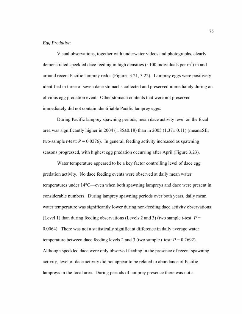
75
Egg Predation
Visual observations, together with underwater videos and photographs, clearly
demonstrated speckled dace feeding in high densities (~100 individuals per m3) in and
around recent Pacific lamprey redds (Figures 3.21, 3.22). Lamprey eggs were positively
identified in three of seven dace stomachs collected and preserved immediately during an
obvious egg predation event. Other stomach contents that were not preserved
immediately did not contain identifiable Pacific lamprey eggs.
During Pacific lamprey spawning periods, mean dace activity level on the focal
area was significantly higher in 2004 (1.85±0.18) than in 2005 (1.37± 0.11) (mean±SE;
two-sample t-test: P = 0.0276). In general, feeding activity increased as spawning
seasons progressed, with highest egg predation occurring after April (Figure 3.23).
Water temperature appeared to be a key factor controlling level of dace egg
predation activity. No dace feeding events were observed at daily mean water
temperatures under 14°C—even when both spawning lampreys and dace were present in
considerable numbers. During lamprey spawning periods over both years, daily mean
water temperature was significantly lower during non-feeding dace activity observations
(Level 1) than during feeding observations (Levels 2 and 3) (two sample t-test: P =
0.0064). There was not a statistically significant difference in daily average water
temperature between dace feeding levels 2 and 3 (two sample t-test: P = 0.2692).
Although speckled dace were only observed feeding in the presence of recent spawning
activity, level of dace activity did not appear to be related to abundance of Pacific
lampreys in the focal area. During periods of lamprey presence there was not a

76
significant difference in the mean number of adult lampreys across dace activity levels
(ANOVA: F2,41 = 1.39, P = 0.2603).
Despite observations of substantial dace predation on lamprey eggs, mean
lamprey survival until emergence was not significantly different among levels of dace
egg predation (ANOVA: F2,14 = 0.33 , P = 0.7248). Likewise, dace predation level was
not significantly different between high survival and low survival cohorts (Table 3.7).
DISCUSSION
SPAWNING ACTIVITY
Pacific lampreys in the South Fork Coquille River spawned between early April
and early June in 2004 (59 d), and over a considerably longer period, from late April until
early July in 2005 (70 d). Estimates of beginning and ending dates of spawning seasons
were similar whether based on adult observations or presence and absence of emergent
ammocoetes; the later always about 20–30 days after initial and final spawner detection.
The April–July spawning period observed on the South Fork Coquille generally agrees
with a March–July season reported in other coastal systems (Kan 1975; Beamish 1980;
Richards 1980; Gunckel et al. 2006). Inland and northern Pacific lamprey populations
are thought to initiate spawning later than coastal populations (Kan 1975; Beamish 1980;
Richards 1980; Close et al. 2003).
In previous years, spawned out individuals have been recovered in the vicinity of
the focal area as early as March 14 (L. Grandmontagne, Wild Fish for Oregon, personal
communication) so it is probable that a small number of fish spawned before we observed

77
them. Elevated river levels prohibited adult surveys prior to early April in 2004 and late
April in 2005. Furthermore, presence of 9–12 mm age-0 ammocoetes in early season
drift samples in 2005 (Figure 3.8) indicate that Pacific lampreys successfully spawned
upstream earlier than predicted from adult surveys. These early spawners were likely
associated with low flows and unseasonably high temperatures that occurred in February
and March of that year (Figure 3.2). This dry and warm late-winter weather likely
resulted in water temperatures warm enough to initiate early spawning. Similarly, the
cool conditions caused by recurrent high flow events, beginning in late March 2005, most
likely arrested spawning activity until daily mean water temperatures warmed above
11°C in late-April. Delayed initiation of Pacific lamprey spawning was also observed in
the Smith River in spring 2005 (Gunckel et al. 2006). The dependence of fish spawning
time on temperature and flow regimes is well established (Pletcher 1963; Hardisty and
Potter 1971b; Kempinger 1988; Reichard et al. 2002a; Dahl et al. 2004).
The finding that Pacific lamprey spawning activity peaked at daily mean water
temperatures between 13°C and 16 ºC is consistent with the range of spawning
temperatures cited in the literature (Pletcher 1963; Kan 1975; Close et al. 2003). The
strong correlations between water temperatures during spawning, water temperature
during development, and discharge during development suggests that embryonic
development conditions may impose strong selective pressure on Pacific lamprey
temperature preference and spawning time. Disruption of these relationships through
alteration of spring temperature and flow regimes could result in a mismatch between
spawning time and conditions for successful embryonic development.

78
LARVAL PRODUCTION
Nearly three times as many emergent ammocoetes were produced in 2004 than in
2005. Although number of spawning adults appears to be a poor predictor of larval
production (Figure 3.13), it is highly likely that lowered production in 2005 was at least
partially due to the three-fold decline in spawners between years.
In both spawning seasons, date of initial and final larval emergence observed
from drift samples largely agreed with that predicted from focal area spawning
observations and degree-days required for emergence. As was expected from cooler
spring water temperatures and prolonged adult spawning in 2005, duration of larval
emergence was more than two weeks longer (71 d) compared to 2004 (54 d). Emergence
peaked around mid-May in 2004 and mid-June in 2005. The greater part of larval
production occurred when mean water temperature during development was 13–17°C and
mean discharge was 150–700 cfs. The lowered larval production associated with higher
water temperatures and lower discharges during development may have been partially
due to decreased embryonic survival, but appeared to be primarily seasonal since these
conditions occurred during the end of the spawning season when few adults spawned.
Young of the year ammocoetes drifted during darkest hours of night, peaking
from 2300 until 0200 hours. Emergent ammocoetes (8–9 mm) drifted, on average, later
than larger and older age-0 larvae (>9 mm), which was likely due to behavioral
differences in drift initiation or spatial differences in point of entry into the drift. The
majority of the 8–9 mm ammocoetes likely originated from redd gravels in the focal area,
whereas older individuals presumably entered the drift from transitory daytime habitats
further upstream. Results from our diel samples concur with previous research showing

79
that ammocoetes display a circadian pattern of drift. In the Great Lakes, drift of
emergent sea lamprey was shown to occur predominately during darkest hours, declining
sharply as dawn approached (Bennett and Ross 1995; Derosier 2001). Similar trends
were detected in drift patterns of mixed age-0 size-classes of Lampetra species (most
likely Pacific lampreys) in Northwest river systems (Pletcher 1963; Gadomski and
Barfoot 1998; White and Harvey 2003). Drifting at night is theorized be an adaptive
response to reduce exposure to visual predators (Muth and Schmulbach 1984; Harvey
1991; Flecker 1992).
There are a number of error sources associated with our estimates of seasonal
production of Pacific lamprey larval from the focal area based on drift samples. First, a
portion of 8–9 mm larvae collected in biweekly nets likely originated from spawning
areas upstream of the focal area. However, the impact of these individual on our results
is considered negligible because of the existence of significant depositional, rearing areas
between the focal spawning area and the nearest upstream spawning area. Furthermore,
adult spawning activity in the 9.2 river kilometers upstream was highly correlated with
focal area spawning activity (see Chapter 2), suggesting that the relative influence of
emergent ammocoetes originating upstream was likely unchanged over time. Similarly,
White and Harvey (2003) found that seasonal trends in ammocoete drift rate were
comparable longitudinally within two Northern California coastal basins.
Second, since spawning western brook lampreys were seen in the focal area in
both years (see Chapter 2), some of their emergent larvae were most likely captured in
the drift. A small pulse of 6–7.5 mm individuals observed in later samples corroborates
this belief (Figure 3.8). Attempts to identify larvae using caudal pigmentation (Richards
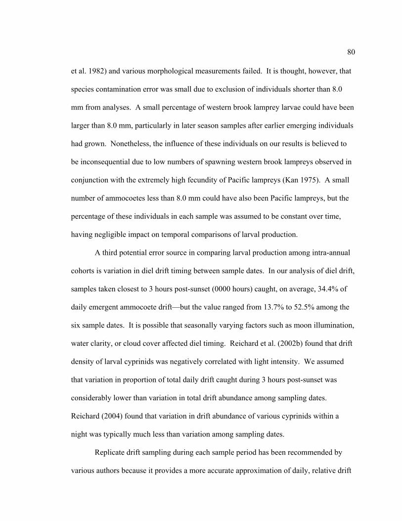
80
et al. 1982) and various morphological measurements failed. It is thought, however, that
species contamination error was small due to exclusion of individuals shorter than 8.0
mm from analyses. A small percentage of western brook lamprey larvae could have been
larger than 8.0 mm, particularly in later season samples after earlier emerging individuals
had grown. Nonetheless, the influence of these individuals on our results is believed to
be inconsequential due to low numbers of spawning western brook lampreys observed in
conjunction with the extremely high fecundity of Pacific lampreys (Kan 1975). A small
number of ammocoetes less than 8.0 mm could have also been Pacific lampreys, but the
percentage of these individuals in each sample was assumed to be constant over time,
having negligible impact on temporal comparisons of larval production.
A third potential error source in comparing larval production among intra-annual
cohorts is variation in diel drift timing between sample dates. In our analysis of diel drift,
samples taken closest to 3 hours post-sunset (0000 hours) caught, on average, 34.4% of
daily emergent ammocoete drift—but the value ranged from 13.7% to 52.5% among the
six sample dates. It is possible that seasonally varying factors such as moon illumination,
water clarity, or cloud cover affected diel timing. Reichard et al. (2002b) found that drift
density of larval cyprinids was negatively correlated with light intensity. We assumed
that variation in proportion of total daily drift caught during 3 hours post-sunset was
considerably lower than variation in total drift abundance among sampling dates.
Reichard (2004) found that variation in drift abundance of various cyprinids within a
night was typically much less than variation among sampling dates.
Replicate drift sampling during each sample period has been recommended by
various authors because it provides a more accurate approximation of daily, relative drift

81
abundance (Allan and Russek 1985; Franzin and Harbicht 1992). In this case, however, a
particularly large drift net [70 x 150 cm opening] was used, which was equivalent to
setting 7.7 typically-sized drift nets [30 x 45 cm opening] simultaneously. Others studies
on drifting invertebrates and fish have shown that a single sample taken near estimated
peak drift time is sufficient to predict total drift from the 24-hr period (Allan and Russek
1984; Zitek et al. 2004).
Finally, our analyses of larval production assumed that observed seasonal drift
patterns corresponded to actual seasonality, not short term fluctuations in emergence
timing. A test comparing drift rate variability of nets set on several consecutive nights to
variability between weekly samples would help substantiate this sampling assumption.
Reichard et al. (2002a) used such a strategy and found no significant differences in drift
densities of several cyprinid species between five successive nights.
Nighttime drift samples have advantages and disadvantages relative to adult and
redd surveys. When adult surveys are impractical due to river size, visibility, or access;
drift nets used in conjunction with a temperature logger and known degree days required
for emergence are an effective way to pinpoint spawning times and provide a continuous
picture of upstream larval production. In rivers where abundance of spawners is low,
drift nets could be used to demonstrate upstream presence when visual adult observations
might not. It is best to sample rare species during parts of the life cycle when their
numbers are great, individuals are vulnerable to quantitative sampling gears, and
individuals can be found over large areas (McDonald 2004). Because of the high
fecundity of Pacific lampreys and associated high larval drift densities, the early life
stages meet these criteria better than other stages.

82
Data on relative larval abundance in the drift can also aid in identification of
productive spawning tributaries and assignment of basinwide conservation priorities
without implementation of spawning surveys. In basins where little information exists,
these techniques allow for rapid collection of diverse information on multiple life stages
and can be used to monitor annual and intra-annual spawning success. In addition to
providing data on various size classes of target lamprey species (Appendices II and III),
drift nets can be used to concurrently collect larval production data on other fish species
(Johnston et al. 1995; White and Harvey 2003). We collected data on five other fish
genera. Disadvantages of drift samples include nighttime work hours, laboratory time,
taxonomic identification problems, difficulty quantifying catches in fluctuating discharge
conditions, and lack of information gained on initial egg production (Allan and Russek
1985; Franzin and Harbicht 1992).
STOCK-RECRUITMENT AND EARLY SURVIVAL
Pacific lamprey spawning success and early mortality was highly variable over
time; as has been documented in numerous other fishes (Kempinger 1988; Hjort, J. 1914;
Harvey 1991; Bestgen and Williams 1994), including lampreys (Hardisty and Potter
1971a; Manion 1968; Derosier 2001; Haesker et al. 2003). On average, number of larvae
produced per spawning adult was similar between years, but there were striking survival
differences relative to spawning time (Tables 3.4, 3.5). Early spawning fish were
generally more successful in 2004 and later spawning fish were more successful in 2005
(Figures 3.14, 3.15). The order of magnitude differences observed in survival between
offspring of early and late spawners is characteristic of highly fecund fishes spawning in

83
unpredictable environments (Houde 1987; Kempinger 1988; Legget and DeBlois 1994;
Pepin 2002). These discrepancies in early life survival were likely due, in part, to
different discharge and water temperature regimes between the two years (Mion et al.
1998; Pitlo 2002; Reichard 2002a), which influenced spawning time, adult density, egg
predation, and interactions among these and other ecological variables affecting egg and
larval survival (Harvey 1991; Johnston et al. 1995; Houde 2002).
At the spawner densities observed in the present study, production of larvae was
positively related to spawning stock on an intra-annual basis. However, spawning stock
explained less than 15% of the variability in larval production, indicating that the
remaining variability can be attributed to embryo mortality after egg deposition. Low
and intermediate abundances of spawners sometimes produced as many or more larvae as
high numbers of spawners (Figures 3.13–3.15). Because of this variability, it is unlikely
that spawning stock can be used to accurately predict year class success until emergence.
Similarly, it is unknown if larval production gives a reliable indication of future
recruitment of out-migrating juveniles, or most importantly returning spawners. Though
higher abundance of newly-hatched larval fish sometimes equate to higher abundance of
older age-classes (Johnston et al. 1995); more commonly, there is little if any relationship
between the two (Partridge and DeVries 1999; Pepin 2002; Pitlo 2002).
The apparent plateau in larval production at higher stock sizes indicates that
habitat saturation may have limited early survival. Results from both univariate (Tables
3.6, 3.7) and AICc regression model selection (Tables 3.8, 3.9) showed that density of
spawning adults was a significant predictor of variability in survival until emergence.
Survival declined with increasing numbers of spawners (Figures 3.18, 3.19), suggesting

84
that density dependence may have limited survival until emergence at elevated spawner
densities through superimposition, or enhanced survival at lower spawner densities via
compensatory mechanisms acting within the redd (Frank and Leggett 1994; Jones et. al
2003). Other potential mechanisms explaining a decline in survival until emergence at
higher spawner densities are density-dependent egg predation or disease. Density-
dependent survival until emergence has not been otherwise documented for Pacific
lampreys. For sea lampreys, Jones et al. (2003) found that recruitment of young-of-the-
year ammocoetes was consistently diminished at large stock sizes, but was widely
variable at low to intermediate stock sizes.
Lowered spawning stock sizes may also trigger compensatory mechanisms after
ammocoetes emergence. Shifts in larval sex ratio towards more females (Zerrenner and
Mardsen 2005), increased larval production and growth rate (Weise and Pajos 1998), and
earlier age at metamorphosis (Jones et al. 2003) have all been cited as examples of post-
swimup compensation in sea lamprey populations following eradication programs.
Increased growth of older Pacific lamprey ammocoetes with decreasing density has also
been documented (Mallat 1983),
While the effects of superimposition have not been directly documented in Pacific
lampreys, they may have contributed to low survival at high spawner densities.
Indication of redd superimposition by later spawning lampreys was observed in early
May of 2004, when, on two occasions, over 25 spawners and remarkably high redd
concentrations were seen in the 30x30 m focal area (Figure 3.4). High densities of
spawners and large areas of disturbed spawning substrate (20x5 m) were also witnessed
during weekly large-scale surveys in May 2004 (see Chapter 2), making individual redds

85
virtually impossible to distinguish. Anecdotal evidence of superimposed spawning by
Pacific lampreys has been cited in previous studies (Pletcher 1963; Kan 1975; Close et al.
2003; Gunckel et al. 2006). Redd superimposition is well recognized as an influential
factor in recruitment of both sea lampreys (Manion and Hanson 1980; Jones et al. 2003)
and anadromous salmonids (Van den Berghe 1989; Fukushima et al. 1998), which spawn
in habitats nearly identical to Pacific lampreys. The potential for inter-specific
superimposition with steelhead, Oncorhynchus mykiss, should also be noted because of
overlap in the species’ spawning seasons. In April and May, we observed steelhead
spawners and redds in the focal area and other lamprey spawning sites.
Discharge during spawning (MDS), or some correlated variable, also played an
important role in Pacific lamprey early life survival in 2004 and 2005: MDS had the
highest relative importance of the predictor variables considered (Table 3.9). Contrary to
the hypothesis that high discharge during spawning would reduce relative survival via
scour or decreased egg deposition, embryo survival generally increased at higher
discharges—even for individuals spawning during spring freshets. For example, larval
production resulting from relatively few fish spawning on the front end of a mid-April
2004 high-water event was among the highest recorded during the period of study
(Figures 3.2, 3.14). Notably, though cohort survival was generally higher at higher
discharges during spawning, it was highly variable below 600 cfs, which suggests that the
relationship was not adequately modeled with linear regression at lower discharges.
Increased survival at high discharges during spawning also questions the
population-level consequences of redd desiccation following high discharge events. In
both years, a number of dried-out Pacific lamprey redds were observed in spawning

86
gravels exposed to the air during rapidly declining river levels following spring freshets.
While these events unquestionably caused extreme mortality for individual redds, their
impact on overall larval cohort survival was not detected and may have been offset by
beneficial factors coupled with high discharge during spawning.
The mechanisms by which discharge during spawning influences Pacific lamprey
spawning success are unclear. Higher flows could elevate survival indirectly due to
lowered water temperature, better interstitial water quality, decreased egg predation, or
reduced redd superimposition resulting from increased size of spawning areas (Johnston
et al. 1995). The latter theory was supported by the significance of the SS*MDS
interaction term in the second ranking regression model (Table 3.8). Survival decline at
the upper range of observed spawner densities suggests that Pacific lampreys in the South
Fork Coquille River may, at times, approach the carrying capacity of available spawning
habitat. If this is the case, increasing available spawning substrate could significantly
bolster larval recruitment. Likewise, if density-dependent recruitment is a generalizable
phenomenon, increased inundation of spawning gravels in the spring may be a viable
management option in regulated rivers.
The apparent unimportance of discharge during development in larval survival
(MDD; Tables 3.7, 3.9) implies that once eggs were safely deposited in redd gravels, they
were relatively unaffected by discharges experienced during this study. Fukushima et al.
(1998) showed negligible loss of eggs from pink salmon redds exposed to freshets after
spawning ceased. Others, however, have documented increased early-life mortality with
increasing discharge (Scrivener et al. 1989; Mion 1998). Since egg size, adhesiveness,

87
and substrate size all interact with flow conditions, the post-spawning relationship
between flow and survival is likely complex and variable over time and between species.
In both years, water temperature tended to increase and discharge declined over
spawning and development periods (Figure 3.10). In spite of the fact that water
temperatures during spawning and development were not significantly correlated with
larval survival at the temperatures ranges observed in this study, the impacts of
temperature on Pacific lamprey early life survival in the wild merit further study. First,
relationships between survival until emergence and water temperature during spawning
and development were not easily modeled using linear regression. Second, even though
survival was highly variable with spawning temperature, only low survival values were
observed at high spawning temperatures (Figure 3.18). There is also evidence that eggs
and larvae of later spawners were exposed to adverse temperature conditions—
particularly in 2004 when daily mean water temperatures commonly surpassed 18ºC and
daily maximums exceeded 25ºC (Figures 3.3, 3.14). These temperatures are considerably
higher than those shown to be detrimental to lamprey embryos in the lab (Meeuwig et al.
2005). Even so, if other factors such as spawner density, discharge, egg predation, or
interactions between these variables reduced survival to a greater magnitude than
temperature, the temperature-related decline in embryo survival observed in a controlled
laboratory setting might not be detected in the wild (Hamor and Garside 1976; Harvey
1991; Pepin 2002).
Although, linear population effects of water temperature were not found,
developing Pacific lamprey embryos in southern parts of their range, as well as in arid,
inland river systems, can be exposed to water temperatures much higher than those
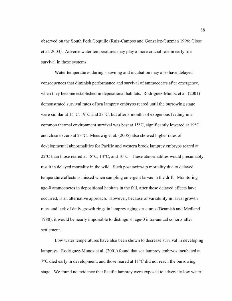
88
observed on the South Fork Coquille (Ruiz-Campos and Gonzalez-Guzman 1996; Close
et al. 2003). Adverse water temperatures may play a more crucial role in early life
survival in these systems.
Water temperatures during spawning and incubation may also have delayed
consequences that diminish performance and survival of ammocoetes after emergence,
when they become established in depositional habitats. Rodriguez-Munoz et al. (2001)
demonstrated survival rates of sea lamprey embryos reared until the burrowing stage
were similar at 15°C, 19°C and 23°C; but after 3 months of exogenous feeding in a
common thermal environment survival was best at 15°C, significantly lowered at 19°C,
and close to zero at 23°C. Meeuwig et al. (2005) also showed higher rates of
developmental abnormalities for Pacific and western brook lamprey embryos reared at
22ºC than those reared at 18°C, 14°C, and 10°C. These abnormalities would presumably
result in delayed mortality in the wild. Such post swim-up mortality due to delayed
temperature effects is missed when sampling emergent larvae in the drift. Monitoring
age-0 ammocoetes in depositional habitats in the fall, after these delayed effects have
occurred, is an alternative approach. However, because of variability in larval growth
rates and lack of daily growth rings in lamprey aging structures (Beamish and Medland
1988), it would be nearly impossible to distinguish age-0 intra-annual cohorts after
settlement.
Low water temperatures have also been shown to decrease survival in developing
lampreys. Rodriguez-Munoz et al. (2001) found that sea lamprey embryos incubated at
7°C died early in development, and those reared at 11°C did not reach the burrowing
stage. We found no evidence that Pacific lamprey were exposed to adversely low water

89
temperatures. Because Pacific lamprey spawning is not initiated until water temperatures
reach 11–12°C and occurs in the spring under a progressively warming temperature
regime, cold water temperatures are unlikely to limit survival in coastal Oregon streams.
Moreover, Pacific lampreys tolerate much lower temperatures regime for spawning and
development than do sea lampreys (Rodriguez-Munoz et al. 2001; Meeuwig et al. 2005).
Developing embryos in this study experienced incubation durations ranging from
18–49 days. Following the logic of the stage duration hypothesis (Leggett and DeBlois
1994), we predicted that longer incubation time would decrease survival by amplifying
the probability of mortality from egg predation, dislodging flows, superimposition,
siltation, or other factors acting on developing embryos. However, our results did not
support this hypothesis: duration of development period (DDP) had no demonstrable
effect on survival until the larval stage over the range of development durations observed
(Table 3.6). On an annual basis Johnston et. al (1995) found no significant effect of
incubation period on year class strength of various freshwater fishes. In contrast, other
studies have cited longer incubation as a root cause of variability in embryo survival
(Rice et al. 1987; Kempinger 1988).
Predation on eggs and larvae is also recognized as a major source of early life
mortality, but its impact is difficult to detect and quantify in the field (Kempinger 1988;
Houde 2002). Though speckled dace were observed feeding in high densities on Pacific
lamprey eggs—particularly later in the 2004 spawning period—we did not detect a
significant influence of predation on relative survival of larval cohorts (Table 3.7). Other
factors acting on survival within the redd may have rendered population-level effects of
dace predation undetectable. Even in the absence of predation, many eggs never reach
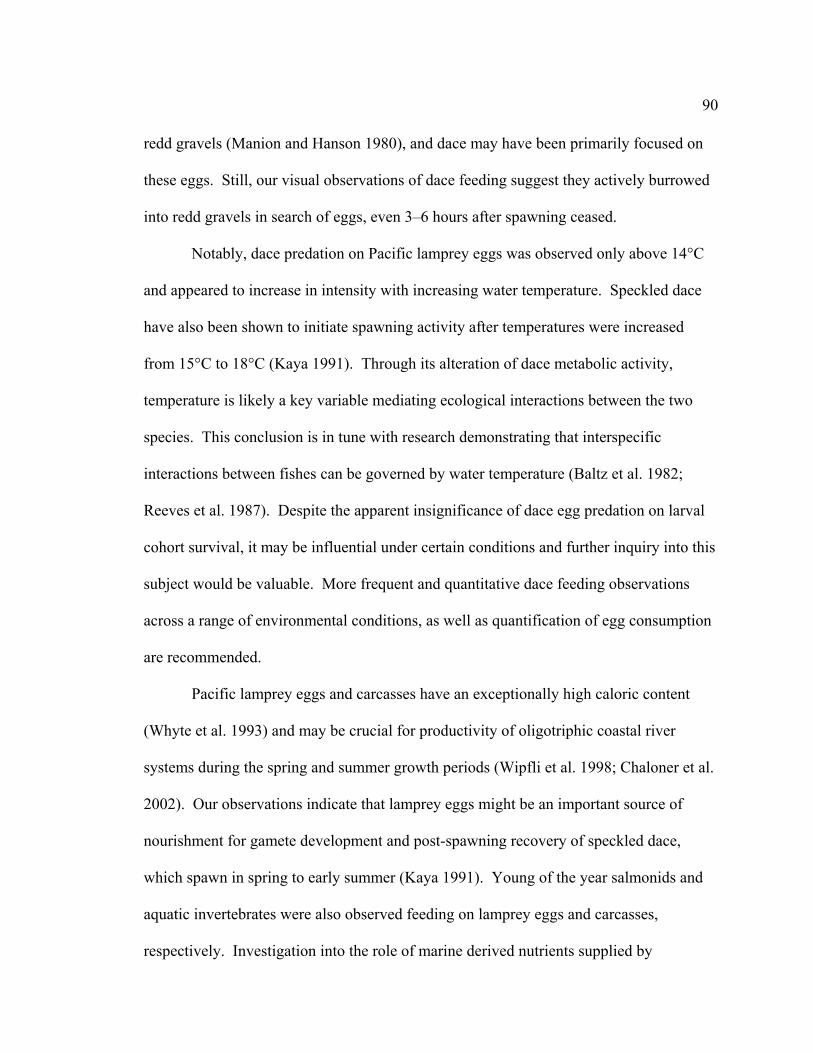
90
redd gravels (Manion and Hanson 1980), and dace may have been primarily focused on
these eggs. Still, our visual observations of dace feeding suggest they actively burrowed
into redd gravels in search of eggs, even 3–6 hours after spawning ceased.
Notably, dace predation on Pacific lamprey eggs was observed only above 14°C
and appeared to increase in intensity with increasing water temperature. Speckled dace
have also been shown to initiate spawning activity after temperatures were increased
from 15°C to 18°C (Kaya 1991). Through its alteration of dace metabolic activity,
temperature is likely a key variable mediating ecological interactions between the two
species. This conclusion is in tune with research demonstrating that interspecific
interactions between fishes can be governed by water temperature (Baltz et al. 1982;
Reeves et al. 1987). Despite the apparent insignificance of dace egg predation on larval
cohort survival, it may be influential under certain conditions and further inquiry into this
subject would be valuable. More frequent and quantitative dace feeding observations
across a range of environmental conditions, as well as quantification of egg consumption
are recommended.
Pacific lamprey eggs and carcasses have an exceptionally high caloric content
(Whyte et al. 1993) and may be crucial for productivity of oligotriphic coastal river
systems during the spring and summer growth periods (Wipfli et al. 1998; Chaloner et al.
2002). Our observations indicate that lamprey eggs might be an important source of
nourishment for gamete development and post-spawning recovery of speckled dace,
which spawn in spring to early summer (Kaya 1991). Young of the year salmonids and
aquatic invertebrates were also observed feeding on lamprey eggs and carcasses,
respectively. Investigation into the role of marine derived nutrients supplied by

91
anadromous lampreys is lacking, but vital for understanding the ecological consequences
of their population decline.
In addition to the explanatory variables considered here, unmeasured factors such
as oxygen concentration, water chemistry (Myllnen et al. 1997), siltation (Kempinger
1988; Meyer 2003), fungal infection (Kempinger 1988; Close 2002), and predation
within the redd (Meyer 2003) may also influence survival until the larval stage. For
example, in coho salmon spawning in similar habitat, Meyer (2003) found that the
amount of fine sediment in the lower half of the egg pocket, which may be related to
presence of a fish egg-eating oligochaete, was a strong predictor of egg survival until
hatching. Research on the European river lamprey, L. fluviatilis, in Finland showed that
hatching success declined markedly with increasing concentrations of iron and aluminum
(Myllynen et al. 1997). The same study showed significant declines in hatching success
and survival of newly hatched ammocoetes at pH levels below 5.5 and 5.0, respectively.
Though adverse water quality has the potential to critically limit Pacific lamprey
reproductive success in systems altered by human activities, its effects on developing
eggs and larvae are unknown.
CONCLUSIONS
Results of regression models employed in this study should be viewed with
caution when drawing inferences about variability in Pacific lamprey early life survival
and recruitment. The explanatory variables shown to be significant are not necessarily
causally related to survival until emergence, but may be correlated to other unknown
factors that are. Likewise, care should be taken when applying conclusions from this

92
study to management of lamprey populations. It is expected that factors important in
determining larval recruitment vary geographically, among habitats, and between years
with dissimilar ecological conditions. Nonetheless, this study offers an important first
step in generating hypotheses about Pacific lamprey stock-recruitment and factors
bearing on early life survival.
Although larval production, stock-recruitment, and early life survival are typically
evaluated on an annual basis (Magnuson 1991; Johnston et al. 1995; Bjorkstedt 2000;
Haeseker 2003), the greater number of data points obtained here by using biweekly
cohorts was advantageous because long term annual data were not available. Using intra-
annual cohorts also allowed us to gain insight on reproductive ecology and factors related
to survival that would not be possible with interannual studies. First, we demonstrated
that timing and magnitude of both, Pacific lamprey spawning and ammocoete production
varied considerably between and within years, and were likely reliant on discharge and
temperature conditions. Second, level of larval production was only marginally
explained by the number of spawning adults, highly variable over the range of stock sizes
observed, and generally diminished at the highest stock sizes. Third, relative survival
until emergence varied greatly between cohorts and was most associated with discharge
conditions during spawning, spawning stock, and an interaction between the two
variables.
These results, along with signs of redd superimposition, suggest that, at higher
stock sizes, larval survival and production may be limited, in part by the amount of
available spawning habitat or other factors related to density-dependence. Because of the
high fecundity of Pacific lampreys and potential for density-dependent compensation

93
(Jones et al. 2003), increases in larval populations may be achieved relatively quickly by
modest gains in spawning and rearing habitats. Conversely, destruction of spawning
habitats is expected to have especially severe consequences by increasing chances of
superimposed spawning. Due to the apparent lack of homing and population subdivision
in Pacific lampreys (Goodman et al. 2006), larval production from a particular river
system is not anticipated to set the baseline for future adult returns of that cohort.
However, through its amplification of the concentration of pheromone-like migratory
attractor substances secreted by ammocoetes (Bjerselius et al. 2000; Vrieze and Sorensen
2001), increased larval production could give rise to improved adult returns on a shorter
time-scale.
Our findings advise against using adult or redd counts as a singular measure of
reproductive success because of the weakness in correlation between spawning stock and
larval recruitment. Spawning surveys are informative with respect to timing and
distribution of reproduction, but they can be misleading because larval production
resulting from a few spawners is sometimes substantially higher than that resulting from
a large number of spawners. Though there are considerable errors associated with
sampling emergent larvae, the technique provides valuable information on intra-annual
and annual larval recruitment than cannot be obtained from spawning surveys. Because
they can be taken in situations when adult counts are not possible, drift samples may
paint a more complete picture of temporal patterns in spawning activity. When feasible,
the multi-life stage approach implemented in this study is recommended because it
provides insight into population-level processes and factors limiting early life survival
that would not be possible when considering adult or larval data independently.

94
TABLES
Table 3.1. Calculation of mean effective degree days (EDD) until the larval stage (stage 18, see Piavis 1961) from laboratory data on Pacific lamprey eggs reared at four constant temperatures. Effective temperature was calculated by subtracting the theoretical temperature for zero development (4.85°C) from rearing temperature.
Rearing Temperature (°C)
Effective Temperature (°C) Days Until Larval Stage EDD
10 5.15 56 288.4 14 9.15 35 320.3 18 13.15 23 302.5 22 17.15 17 291.6
mean 300.7 Note: days until the larval stage and the theoretical temperature for zero development were obtained from Meeuwig et al. (2005). Table 3.2. Variables employed in simple and multiple linear regression models explaining loge larval drift rate per adult (survival until emergence) for intra-annual cohorts and associated symbols. Explanatory Variable Symbol
Number of adult Pacific lamprey present in spawning period1,2 SS
Mean water temperature during development period1,2 MWTD
Number of days daily mean water temperature exceeds 20°C1 DMWT20+
Mean water temp during spawning period1,2 MWTS
Discharge during drift sample1 Discharge
Mean discharge during development period1,2 MDD
Number of days daily mean discharge exceeded 1000 cfs1 DMD1000+
Mean discharge during spawning period1,2 MDS
Fraction of moon illuminated during drift sample1,2 FMI
Duration of development period1,2 DDP
Year (indicator variable)1,2 Year SS*MDS Interaction Term2 SS*MDS
1Denotes variable used in simple linear regression. 2Denotes variable used in multiple linear regression model selection.

95
Table 3.3. Total number of age-0 ammocoetes caught at focal area in biweekly and diel samples by size-class in 2004 and 2005; N = number of net samples. Net samples from small nets consisted of two small nets stacked to cover the water column.
2004 2005 Sample Type Gear N <8 mm 8–9
mm >9 mm N <8 mm 8–9 mm >9 mm
Biweekly Large Net 26 110 3791 3000 27 67 1355 1432
Diel Small Nets 48 213 837 192 16 64 583 380
Total 74 323 4628 3192 43 131 1938 1812
Table 3.4. Relative annual survival until the larval phase for Pacific lampreys in 2004 and 2005. Total Annual Larval Production equals the annual sum of emergent ammocoete drift rates from all biweekly nets. Number of Spawners is the estimated number of mature adults present in the focal area during spawning periods corresponding to biweekly larval cohorts. Relative Survival Index equals Total Annual Larval Production divided by Number of Spawners.
Measure 2004 2005
Total Annual Larval Production 5652.5 2017.8
Number of Spawners 369.8 177.7
Relative Survival Index 15.3 11.4
Table 3.5. Percent of Pacific lampreys spawning in each month, percent of larval production resulting from each month’s spawners, and monthly Index of Survival (calculated by dividing percent of larvae by percent of spawners) for 2004 and 2005. Within each year, Index of Survival values greater than 1.0 are considered above average and lower than 1.0 below average.
2004 2005
Spawning Month
Percent of Spawners
Percent of Resultant Larvae
Index of Survival
Percent of Spawners
Percent of Resultant Larvae
Index of Survival
March 0.0 0.0 na 0.0 0.1 na
April 27.9 64.6 2.3 25.9 7.3 0.3
May 70.8 35.0 0.5 46.6 65.6 1.4
June 1.3 0.3 0.3 26.7 26.9 1.0
July 0.0 0.0 na 0.7 0.0 0.0

96
Table 3.6. Results of simple linear regression models explaining survival until emergence (loge larval drift rate per adult; df = 25). Note: r2 values and coefficient values are only listed for models with P < 0.15. See Table 3.1 for description of variable symbols. Variable P r2 Coefficient Value
SS ln 0.0091 0.251 -0.583 MWTD 0.7378 DMWT20+ 0.5435 MWTS 0.1041 0.106 -0.246 Discharge ln 0.7259 MDD ln 0.6752 DMD1000+ 0.6492 MDS 0.0033 0.307 0.002 FMI 0.3986 DDP 0.9576 Year 0.7238
ln Denotes variable loge transformed before regression. Table 3.7. Comparison of mean values of explanatory variables between the highest 50% (N=13) and lowest 50% (N=13) of intra-annual-cohort survival values from 2004 and 2005 combined data. P-values were derived from two sample t-tests. See Table 3.1 for description of variable symbols.
Low Survival High Survival
Variable Mean value SE
Mean Value SE P-Value
*SS 25.28 6.407 9.43 2.599 0.0310 MWTD 15.38 0.553 14.97 0.508 0.5874
DMWT20+ 1.38 0.781 1.23 0.579 0.8756 MWTS 14.60 0.529 13.41 0.538 0.1285
Discharge 194.31 29.091 290.15 66.416 0.1987 MDD 364.54 64.036 448.15 59.416 0.3480
DMD1000+ 2.15 0.933 2.92 0.880 0.5543 *MDS 318.55 32.744 674.24 154.943 0.0342 FMI 0.47 0.084 0.30 0.093 0.2053 DDP 28.54 1.509 29.54 1.444 0.6364
Dace Activity Level 1.69 0.249 1.56 0.258 0.7323 *Significantly different between low and high survival levels

97
Table 3.8. Top ten linear regression models describing relative Pacific lamprey survival until emergence; selected from AICc analysis. Akaike weight was calculated from all 145 candidate models (N = 26 for all models). Model: Survivalln = function of: L(θ) K AICc ΔAICc e^
(-½ΔAICc)
Akaike weight
(w) R2
1) SSln, MDS -2.496 4 14.897 0.000 1.000 0.102 0.435 ┼2) SSln, MDS, Year -1.180 5 15.359 0.462 0.794 0.081 0.489 ┼3) SSln, MDS, SS*MDS -1.561 5 16.122 1.225 0.542 0.055 0.474 4) SSln, MDS, FMI -2.169 5 17.339 2.441 0.295 0.030 0.449 5) MDS -5.134 3 17.358 2.461 0.292 0.030 0.307 6) SSln, MDDln, MDS -2.304 5 17.607 2.710 0.258 0.026 0.443 7) SSln, MDS, DDP -2.365 5 17.729 2.832 0.243 0.025 0.440 8) MDS, FMI -4.008 4 17.920 3.022 0.221 0.023 0.365 9) SSln, MWTS, MDS -2.468 5 17.937 3.039 0.219 0.022 0.436 10) SSln, MWTD, MDS -2.496 5 17.992 3.095 0.213 0.022 0.435
ln Denotes variable loge transformed before regression. ┼considered competing with top model. Table 3.9. Relative importance values of variables used to predict survival until emergence. Calculated from Akaike weights of the 145 candidate models. See Table 3.1 for description of variable symbols. Model Parameter Relative Importance Value MDS 0.850 SS 0.765 Year 0.327 FMI 0.256 MWTS 0.239 DDP 0.174 SS*MDS 0.169 MDD 0.152 MWTD 0.127

98
FIGURES
Figure 3.1. Location of focal spawning area in relation to the large-scale survey section (see Chapter 2) and the Coquille River Basin, Oregon.

99
Figure 3.2. 2004 and 2005 discharge (cubic feet per second) on South Fork Coquille River from January 1 to July 30.
Figure 3.3. Daily mean water temperature at the focal area from April 4 until August 3, 2004 and 2005.

100
Figure 3.4. Seasonal distribution of adult Pacific lampreys in the focal spawning area in 2004. The arrow indicates a period of high discharge when sampling was not possible. Stars represent observations when zero fish were seen.
Figure 3.5. Seasonal distribution of adult Pacific lampreys in the focal spawning area in 2005. Arrows indicate periods of high discharge when sampling was not possible. Stars represent observations when zero fish were seen. Note the difference in y-axis scale between Figures 3.4 and 3.5.

101
Figure 3.6. Number of mature adult Pacific lampreys on the focal area versus daily mean water temperature in 2004 and 2005.
Figure 3.7. Number of mature adult Pacific lampreys on the focal area versus daily mean discharge during observations in 2004 and 2005.

102
Figure 3.8. Age-0 lamprey drift rates in 2004 and 2005 for emergent ammocoetes (8–9 mm), ammocoetes greater than 9 mm, and those less than 8 mm. Note the difference in the y-axis scale between years.
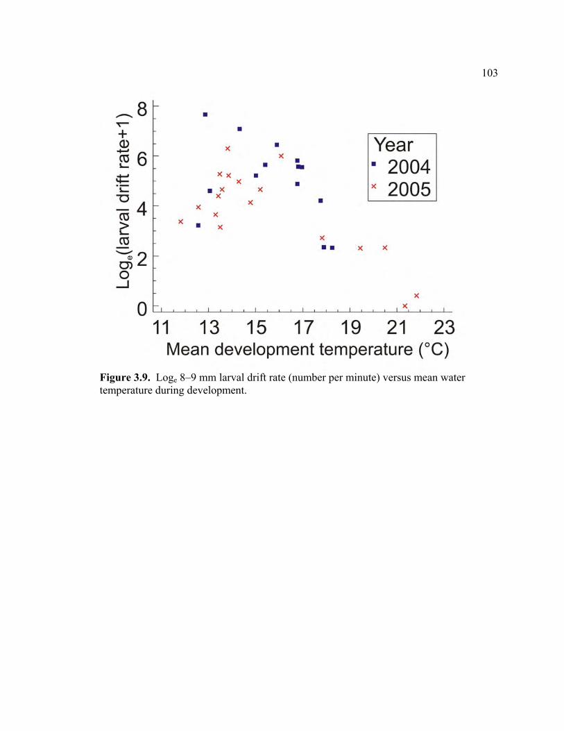
103
Figure 3.9. Loge 8–9 mm larval drift rate (number per minute) versus mean water temperature during development.

104
Figure 3.10. Seasonal production of emergent larvae (number per minute) and mean water temperature and discharge during corresponding developmental periods in 2004 and 2005.

105
Figure 3.11. Loge 8–9 mm larval drift rate (number per minute) versus mean discharge during development.
Figure 3.12. Percent drift density at each net-time for age-0 ammocoetes captured during diel samples. Averaged over 6 sampling cycles; 2004 and 2005 samples combined. Bars represent standard errors.

106
Figure 3.13. Relationship between larval production (8–9 mm ammocoete drift rate) and spawning stock (adult count estimates from corresponding spawning period).

107
0
5
10
15
20
25
30
35
403/
24-3
/27
4/2-
4/4
4/4-
4/7
4/9-
4/12
4/13
-4/1
7
4/21
-4/2
5
4/27
-4/3
0
5/2-
5/5
5/6-
5/9
5/11
-5/1
4
5/16
-5/1
8
5/19
-5/2
1
5/22
-5/2
5
5/28
-5/3
1
6/1-
6/3
6/5-
6/8
6/10
-6/1
3
Corresponding spawning period
Perc
ent o
f lar
vae
or a
dults
5/6/
2004
5/11
/200
4
5/13
/200
4
5/17
/200
4
5/20
/200
4
5/24
/200
4
5/27
/200
4
5/31
/200
4
6/3/
2004
6/6/
2004
6/10
/200
4
6/13
/200
4
6/16
/200
4
6/21
/200
4
6/24
/200
4
6/28
/200
4
7/1/
2004
Larval Emergence Date
AdultsEmergent larvae
Figure 3.14. Percent of 2004 emergent larval production collected during drift samples overlaid on percent of annual adult observations from corresponding spawning periods. Differences between magnitude of percent adults and percent emergent larvae represent relative survival until emergence.
0
5
10
15
20
25
30
3/26
-3/3
04/
2-4/
54/
8-4/
134/
15-4
/21
4/24
-4/2
74/
28-4
/30
5/3-
5/4
5/5-
5/7
5/8-
5/11
5/12
-5/1
55/
16-5
/18
5/21
-5/2
45/
28-5
/30
5/31
-6/3
6/6-
6/10
6/16
-6/2
06/
23-6
/26
6/27
-6/3
07/
3-7/
57/
7-7/
107/
11-7
/13
Corresponding spawning period
Per
cent
larv
ae o
r adu
lts
5/15
/05
5/19
/05
5/23
/05
5/26
/05
5/30
/05
6/2/
056/
6/05
6/9/
056/
12/0
56/
15/0
56/
18/0
56/
22/0
56/
27/0
56/
30/0
57/
4/05
7/10
/05
7/14
/05
7/17
/05
7/21
/05
7/25
/05
7/28
/05
Larval emergence date
AdultsEmergent larvae
Figure 3.15. Percent of 2005 emergent larval production collected during drift samples overlaid on percent of annual adult observations from corresponding spawning periods. Differences between magnitude of percent adults and percent emergent larvae represent relative survival until emergence.

108
Figure 3.16. Relationship between relative survival until emergence (emergent larval drift rate per corresponding adult) and mean discharge during the spawning period (r2 = 0.307; P = 0.0033; N = 26).
Figure 3.17. Relationship between relative survival until emergence (emergent larval drift rate per corresponding adult) and number of adults present in the corresponding spawning period (r2 = 0.252; P = 0.0091; N = 26).

109
Figure 3.18. Relationship between relative survival until emergence (emergent larval drift rate per corresponding adult) and mean water temperature during the spawning period.
Figure 3.19. Comparison of mean discharge during spawning between the highest 50% (N=13) and lowest 50% (N=13) of intra-annual larval cohort survival values.

110
Figure 3.20. Comparison of spawning stock between the highest 50% (N=13) and lowest 50% (N=13) of intra-annual larval cohort survival values.

111
Figure 3.21. Examples of speckled dace feeding behavior. The photograph on the left illustrates an individual dace burrowing into redd gravels in search of lamprey eggs. The photo on the right was taken immediately downstream of a recently spawned-in Pacific lamprey redd.
Figure 3.22. Photographic documentation of high densities of speckled dace preying on eggs during Pacific lamprey spawning. Each white arrow represents a visible, individual dace (N = 76). The area in the photograph is approximately 1 m2.

112
Figure 3.23. Monthly means and standard errors of speckled dace relative feeding level during 2004 and 2005 Pacific lamprey spawning periods.

113
CHAPTER 4
SUMMARY AND CONCLUSIONS
The 2003 petition for Endangered Species Act (ESA) listing of the Pacific
lamprey, Lampetra tridentata, has highlighted data gaps in its basic biology and
management in the northwestern United States, particularly in early life stages and
population monitoring. This study investigated Pacific lamprey spawning and larval
recruitment patterns in a coastal Oregon stream in 2004 and 2005.
Chapter 2 evaluated spatial and temporal aspects of adult and redd surveys and
documented spawning and residence times, length frequency, sex ratio, and movement in
the Coquille River. Residence time on spawning grounds was less than one week and
declined as the season progressed. The interpretation of adult data is, therefore, sensitive
to the frequency of surveys which, ideally, should be carried out more often than weekly.
A more focused tagging study of residence times of both sexes would be valuable for
determining the most useful survey frequency.
When spawner abundance was high, seasonal patterns in spawning activity were
highly correlated at three spatial scales: a 9.2 km river section, individual reaches within
that section, and a single spawning area downstream. Consequently, when resources are
scarce it may be better to have more frequent samples of a small area than fewer samples
of a large area. However, in this study habitat conditions were comparable among river
sections, and such spatial correlations may not hold in other river systems. For this
reason, additional evaluations of spawning activity over time and space would be useful
for testing assumptions about scale of observation required for informative annual

114
monitoring. Lastly, adult and redd counts suffer from errors due to observer variability,
movement during surveys, night spawning, and variable visibility related to weather and
flow. To make spawning surveys more effective tools for population monitoring, these
errors need to be better quantified. Since long-term population monitoring is important
for understanding species status and response to management actions, future studies
should evaluate the meaning of adult and redd count data with respect to both adult
escapement and recruitment of future generations.
In Chapter 3 we described seasonal variation in spawning time and larval
production, evaluated the stock-larval recruitment relationship, and investigated potential
limitations to early life survival. We demonstrated that timing and magnitude of Pacific
lamprey spawning and ammocoete production varied greatly between and within years,
and were likely dictated by temperature and discharge conditions. Spawning stock
explained <15% of the variability in larval production, indicating that gains in egg
production at higher stock sizes were offset by increased embryo mortality. As expected,
survival until larval emergence varied greatly between intra-annual cohorts. Survival was
significantly related to spawning stock size, discharge during spawning, and their
interaction and generally declined with increasing spawning stock and decreasing
discharge. These relationships could due to constriction of spawning habitat associated
with falling river-levels. These results, as well as investigations into Great lakes sea
lamprey population dynamics (Jones et al. 2003; Haesker et al. 2003), point to density-
dependent survival and suggest that larval production may be limited by spawning
habitat. If this is the case, restoration of degraded spawning habitats or maintenance of
flow during the spawning season via dam releases or decreased water withdrawals, could

115
result in increased larval production. Although density-dependent survival and
recruitment is well established for some populations of anadromous salmonids (Van den
Berghe 1989; Fukushima et al. 1998) and sea lampreys (Weise and Pajos 1998; Jones et
al. 2003; Haesker et al. 2003), more controlled studies of Pacific lamprey populations are
needed. Specifically, evaluation of the effect of spawning-stock size on larval production
across a range of well-quantified spawning habitat sizes and/or conditions would be
valuable. Likewise, longer term studies to monitor spawning populations, emergent
larvae, and older age-classes over a range of environmental conditions are needed to
better understand recruitment processes. When feasible, the multi-life stage approach
implemented in this study is recommended because it allows for greater insight into
population dynamics and limiting factors than adult or larval data alone.

116
LITERATURE CITED
Allan and Russek. 1985. The quantification of stream drift. Canadian Journal of Fisheries and Aquatic Sciences 42:210–215.
Al-chokhachy R., P. Budy, and H. Schaller. 2005. Understanding the significance of redd counts: a comparison between two methods for estimation the abundance of and monitoring bull trout populations. North American Journal of Fisheries Management 25:1505–1512.
Alderdice, D.F., and F.P.J Velsen. 1978. Relationship between temperature and incubation time for eggs of chinook salmon (Oncorhynchus tshawytscha). Journal of the Fisheries Research Board of Canada 35:69–75.
Baltz, D.M., P.B. Moyle, and N.J. Knight. 1982. Competitive interactions between benthic stream fishes, rifle sculpin, Cottus gulosus, and speckled dace, Rhinichthys osculus. Canadian Journal of Fisheries and Aquatic Sciences 39:1502–1511.
Bayer, J.M., T.C. Robinson and J.G. Seelye. 2001. Upstream migration of Pacific Lampreys in the John Day River: Behavior, timing and habitat use. Annual Report for 2000. Bonneville Power Administration Project Number 2000-052. Portland, Oregon. http://www.efw.bpa.gov/Publications/I26080-1.pdf
Bennett, R.M. and R.M. Ross. 1995. Stream drift of newly hatched sea lampreys in the upper Delaware River. Journal of the Pennsylvania Academy of Science 69(1):7–9.
Benoît, H.P. and Pepin, P. 1999. Interaction of rearing temperature and maternal influence on egg development rates and larval size at hatch in yellowtail flounder (Pleuronectes ferrugineus). Canadian Journal of Fisheries and Aquatic Sciences, 56: 785–794.
Beamish, R.J. 1980. Adult biology of the River Lamprey (Lampetra ayresi) and the Pacific Lamprey (Lampetra tridentata) from the Pacific coast of Canada. Canadian Journal of Fisheries and Aquatic Science 37: 1906–1923.
Beamish, F. W. H., and T. E. Medland. 1988. Age determination for lampreys. Transactions of the American Fisheries Society 117:63–71.
Beamish, R.J. and C. D. Levings. 1991. Abundance and freshwater migrations of the anadromous parasitic lamprey, Lampetra tridentata, in a tributary of the Fraser River, British Columbia. Canadian Journal of Fisheries and Aquatic Sciences. 48:1250–1263.
Bergstedt, R.A., and J.G. Seelye. 1995. Evidence for lack of homing by sea lampreys. Transactions of the American Fisheries Society 124:235–239.
Bestgen K.R., and M.A. Williams. 1994. Effects of fluctuating and constant temperatures on early development and survival of Colorado squawfish. Transactions of the American Fisheries Society 123:574–579.
Bjerselius, R., W. Li, J. H. Teeter, J. G. Seelye, P. B. Johnsen, P. J. Maniak, G. C. Grant, C. N. Polkinghorne, and P. W. Sorensen. 2000. Direct behavioral evidence that unique bile acids released by larval sea lamprey (Petromyzon marinus) function as a migratory pheromone. Canadian Journal of Fisheries and Aquatic Sciences 57:557–569.

117
Bjorkstedt, E.P. 2000. Stock–recruitment relationships for life cycles that exhibit concurrent density dependence. Canadian Journal of Fisheries and Aquatic Sciences 57: 459–467.
Burnham, K. P., and D. R. Anderson. 1998. Model selection and inference: a practical information-theoretic approach. Springer-Verlag, New York, New York, USA. 353 pp.
Byram, R.S. Scoquel, Coquelle, and Coquille. 2002. Pages 121–138 in D.B. Ivy and R.S. Byram, editors. Changing landscapes: sustaining traditions. Proceedings of the 5th and 6th Annual Coquille Cultural Preservation Conferences. Coquille Indian Tribe, North Bend, Oregon.
CRBLTW (Columbia River Basin Lamprey Technical Workgroup) 2005. Critical Uncertainties for Lamprey in the Columbia Basin: Results from a strategic planning retreat of the Columbia River Technical Workgroup, Columbia Basin Fish and Wildlife Authority, Portland OR. http://www.fws.gov/columbiariver/lampreywg/docs/CritUncertFinal.pdf
Chaloner, D. T., K. M. Martin, M. S. Wipfli, P. H. Ostrom, and G. A. Lamberti. 2002. Marine carbon and nitrogen in southeastern Alaska stream food webs: evidence from artificial and natural streams. Canadian Journal of Fisheries and Aquatic Sciences 59:1257–1265.
Close, D.A., M. Fitzpatrick, H. Li, B. Parker, D. Hatch, and G. James. 1995. Status report of the Pacific Lamprey (Lampetra tridentata) in the Columbia Basin. Bonneville Power Administration Project Number 94-026. Portland, Oregon. http://www.efw.bpa.gov/Publications/I39067-1.pdf
Close, D.A., M.S. Fitzpatrick, and H.W. Li. 2002. The ecological and cultural importance of a species at risk of extinction, Pacific Lamprey. Fisheries 27(7):19–25
Close, D.A. 2002. Pacific Lamprey Research and Restoration Project: Annual Report for 2001. Bonneville Power Administration Project Number. 1994-026. Portland, Oregon. http://www.efw.bpa.gov/Publications/I00005455-3.pdf
Close, D.A., K. Aronsuu, A. Jackson, T. Robinson, J. Bayer, J. Seelye, S. Yun, A. Scott, W. Li, C. Torgersen. 2003. Pacific Lamprey Research and Restoration Project: Annual Report for 2002. Bonneville Power Administration Project Number. 1994-026. Portland, Oregon. http://www.efw.bpa.gov/Publications/I00005455-6.pdf
Close, D.A., A.D. Jackson, B.P. Conner, and H.W. Li. 2004. Traditional Ecological Knowledge of Pacific lamprey (Entosphenus tridentatus) in Northeastern Oregon and Southeastern Washington from indigenous peoples of the Confederated Tribes of the Umatilla Indian Reservation. Journal of Northwest Anthropology 38(2):141–162.
Cochnauer, T., C. Claire., and S.A. Putnam. 2006. Evaluate Status of Pacific lamprey in the Clearwater River Drainage, Idaho. Annual Report for 2005. Bonneville Power Administration Project Number 2000-028. Portland, Oregon. http://www.efw.bpa.gov/Publications/I00020623-1.pdf
CRBLTW (Columbia River Basin Lamprey Technical Workgroup). 2005. April 19. Critical uncertainties for lamprey in the Columbia River Basin: results from a strategic planning retreat of the Columbia River Lamprey Technical Workgroup. http://www.fws.gov/columbiariver/lampreywg/docs/CritUncertFinal.pdf

118
Dahl, J., J. Dannewitz, L. Karlsson, E. Petersson, A. Löf, and, B. Ragnarsson. 2004. The timing of spawning migration: implications of environmental variation, life history, and sex. Canadian Journal of Zoology 82(12): 1864–1870.
Derosier, A.L. 2001. Early life history of sea lamprey: emergence, movements, and dispersal. Masters of Science Thesis. Michigan State University. East Lansing, Michigan. 80 pp.
Docker, M. F., J. H. Youson, R. J. Beamish, and R. H. Devlin. 1999. Phylogeny of the lamprey genus Lampetra inferred from mitochondrial cytochrome b and ND3 gene sequences. Canadian Journal of Fisheries and Aquatic Sciences 56:2340–2349.
Dunham, J. and B. Rieman. 2001. Sources and magnitude of sampling error in redd counts for bull trout. North American Journal of Fisheries Management 21:343–352.
Elliot. J.M. 1989. Mechanisms responsible for population regulation in young migratory trout, Salmo trutta. I. The critical time for survival. The Journal of Animal Ecology 58:987-1001.
Farlinger S.P. and R.J. Beamish 1984. Recent colonization of a major salmon-producing lake in British Columbia by Pacific lamprey. Canadian Journal of Fisheries and Aquatic Science 41:278–285.
Flecker, A.S. 1992. Fish predation and the evolution of invertebrate drift periodicity: evidence from neotropical streams ecology 73(2):438–448.
Frank, K.T. and W.C. Leggett. 1994. Fisheries ecology in the context of ecological and evolutionary theory. Annual Review of Ecology and Systematics 25:401–422.
Franzin W.G. and S.M. Harbicht. 1992. Tests of drift samplers for estimating abundance of recently hatched walleye larvae in small rivers. North American Journal of Fisheries Management 12:396–405.
Fukushima, M., T.J. Quinn, and W.W. Smoker. 1998. Estimation of eggs lost from superimposed pink salmon (Oncorhynchus gorbuscha) redds. Canadian Journal of Fisheries and Aquatic Sciences 55:618–625.
Gadomski, D.M. and C.A. Barfoot. 1998. Diel and distributional abundance patterns of fish embryos and larvae in the lower Columbia and Deschutes rivers. Environmental Biology of Fishes 51:353–368.
Gale, W. F., and H. W. Mohr, Jr. 1978. Larval fish drift in a large river with a comparison of methods. Transactions of the American Fisheries Society 107:46–55.
Goodman, D., S. Reid, and M. Docker. 2006. A phylogeographic analysis of the Pacific lamprey Entosphenus tridentatus. Revised Final Project Report for U.S. Fish and Wildlife Service. Contract Purchase Order # 10181-4-M465. Portland, Oregon
Graham, J.C. and C.V. Brun. 2005. Determining lamprey species composition, larval distribution, and adult abundance in the Deschutes River, Oregon, Subbasin. Bonneville Power Administration. Annual Report for 2004. BPA Project Number 2002-016. Portland, Oregon. http://www.efw.bpa.gov/Publications/I00009553-3.pdf

119
Gunckel, S.L., K.K. Jones, and S.E. Jacobs. 2006. Spawning distribution and habitat use of adult Pacific and western brook lamprey in Smith River, Oregon. Fish Division, Oregon Department of Fish and Wildlife. Information Reports Number 2006-1. Report to U.S. Fish and Wildlife Service. Wildlife Conservation and Restoration, Contract R-5-1. Portland, Oregon.
Hardisty, M.W. and I.C. Potter. 1971a. The behavior, ecology and growth of larval lampreys.. IN The Biology of Lampreys (1): 85–125. M. W. Hardisty and I. C. Potter (ed.). Academic Press, London.
Hardisty, M.W. and I.C. Potter. 1971b. The general biology of adult lampreys. IN The Biology of Lampreys (1): 127–206. M. W. Hardisty and I. C. Potter (ed.). Academic Press, London.
Haesker, S.L., M.L. Jones, and J.R. Bence. 2003. Estimating uncertainty in the stock- recruitment relationship for St. Marys River sea lampreys. Journal of Great Lakes Research 29 (Supplement 1): 728–741.
Hamel, P., P. Magnan, P. East, M. Lapointe, P. Laurendeau. 1997. Comparison of different models to predict the in situ embryonic developmental rate of fish, with special reference to white sucker (Catostomus commersoni). Canadian Journal of Fisheries and Aquatic Sciences 54:190–107.
Hamor, T., and E.T. Garside. 1976. Developmental rates of embryos of Atlantic salmon, Salmo salar L., in response to various levels of temperature, dissolved oxygen, and water exchange. Canadian Journal of Zoology 54:1912–1917.
Harvey, B. C. 1991. Interaction of abiotic and biotic factors influences larval fish survival in an Oklahoma stream. Canadian Journal of Fisheries and Aquatic Sciences 48:1476–1480.
Hjort, J. 1914. Fluctuations in the great fisheries of northern Europe. Rapport du Conseil d’Exploration de Mer 20:1–228.
Hoffman, J.C. and J.E. Olney. 2005. Cohort-specific growth and mortality of juvenile American shad in the Pamunkey River, Virginia. Transactions of the American Fisheries Society 134:1–18.
Houde, E. D. 1987. Fish early life dynamics and recruitment variability. Pages 17–29 in R. D. Hoyt, editor. 10th Annual Larval Fish Conference. American Fisheries Society, Symposium 2, Bethesda, Maryland.
Houde, E.D. 2002. Mortality. Pages 64–87 in L.A. Fuiman and R.G. Werner, editors. Fishery science: the unique contributions of early life stages. Blackwell Science, Oxford.
Howard J. K., D.A. Close., and A.D. Jackson 2005. Pacific Lamprey Research and Restoration Project: Annual Report for 2004. Bonneville Power Administration Project Number 1994-026. Portland, Oregon.
http://www.efw.bpa.gov/Publications/I00005455-8.pdf Hubbs, C.L. and I.C. Potter. 1971. Distribution, phylogeny and taxonomy. IN The
Biology of Lampreys (1): 1–65. M. W. Hardisty and I. C. Potter (ed.). Academic Press, London.
Humphries, P.K., and A.J. Koehn, J.D. Fish. 1999. Flows and flood plains: links between freshwater fishes and their environment in the Murray-Darling River System, Australia. Environmental Biology of Fishes 56:129–151.

120
Hurvich, C. M., and C.L. Tsai. 1989. Regression and time series model selection in small samples. Bometrika 76:297–307.
John, K.R. and A.D Hasler. 1956. Observations of some factors affecting the hatching of eggs and the survival of young shallow-water cisco, Leucichthys artedi LeSuer, in Lake Mendota Wisconsin. Limnology and Oceanography 1(3):176–194.
Johnston, T.A., M.N. Gaboury, R.A. Janusz, and L.R. Janusz. 1995. Larval fish drift in the Valley River, Manitoba: influence of abiotic and biotic factors, and relationships with future year-class strengths. Canadian Journal of Fisheries and Aquatic Sciences 52:2423–2431.
Jones, M.L., R.A. Bergstedt, M.B. Twhoey, M.F. Fodale, D.W. Cuddy, and J.W. Slade. 2003. Compensatory mechanisms in Great Lakes sea lamprey populations: implication for alternative control strategies. Journal of Great Lakes Research 29 (Supplement 1):113–129.
Kan, T.T. 1975. Systematics, variation, distribution, and biology of lampreys of the genus Lampetra in Oregon. Dissertation for the Doctor of Philosophy. Oregon State University, Corvallis, Oregon. 194 pp.
Kaya, C.M. 1991. Laboratory spawning and rearing of speckled dace. The Progressive Fish-Culturist 53:259–260.
Kempinger, J.J. 1988. Spawning and early life history of lake sturgeon in the Lake Winnebago system, Wisconsin. Pages 110–122 in R.D. Hoyt, editor. 11th Annual Larval Fish Conference. American Fisheries Society, Symposium 5, Houghton, Michigan.
Kostow, K. 2002. Oregon Lampreys: Natural history, status, and problem analysis. Edited on April 21, 2003. Oregon Department of Fish and Wildlife, Portland, OR.
http://nrimp.dfw.state.or.us/nrimp/information/docs/fishreports/FinalOregonLampreysReport.pdf
Larson, Z.S. and M.R. Belchik. 1998. A preliminary status review of eulachon and Pacific lamprey in the Klamath River Basin. Yurok Tribal Fisheries Program, Klamath, California.
Leggett, W. C., and E. DeBlois. 1994. Recruitment in marine fishes: is it regulated by starvation and predation in the egg and larval stages? Netherlands Journal of Sea Research 32:119–134.
Lorion, C, D. F. Markle, S. Reid, and M. Docker 2000. Re-description of the presumed- extinct Miller Lake lamprey, Lampetra minima. Copeia 4:1019–1028.
Luzier, C.W., and G. Silver. 2005. Evaluate habitat use and population dynamics of lampreys in Cedar Creek, Annual Report 2004. Bonneville Power Administration. Annual Report for 2004. BPA Project Number 2000-140. Portland, Oregon. http://www.efw.bpa.gov/Publications/I00004672-4.pdf
Magnuson, J.J. 1991. Fish and fisheries ecology. Ecological Applications 1(1):13–26 Malmqvist, B. 1986. Reproductive ecology of lampreys. Pages 20–30 in T. Uyeno, R.
Arai, T. Taniuchi, and K. Matsuura, editors. Indo-Pacific fish biology: Proceedings of the second international conference on Indo-Pacific fishes. Icthyological Society of Japan, Tokyo.
Mallatt, J. 1983. Laboratory growth of larval lampreys (Lampetra (Entosphenus) tridentata Richardson) at different food concentrations and animal densities. Journal of Fish Biology 22:293–301.

121
Manion, P.J. 1968. Production of sea lamprey larvae from nests in two Lake Superior streams. Transactions of the American Fisheries Society 97: 484–48.
Manion, P.J., and L.H. Hanson. 1980. Spawning behavior and fecundity of lampreys from the upper three Great Lakes. Canadian Journal of Fisheries and Aquatic Sciences 37:1635–1640.
McDonald, L. L. 2004. Sampling rare populations, pages. 11–42. in W. L. Thompson, editor. Sampling rare or elusive species. Island Press, Washington, 429 pp.
Meeuwig, M.H., J.M. Bayer, and R.A. Reiche. 2004. Identification of larval Pacific lampreys (Lampetra tridentata), river lampreys (L. ayresi), and western brook lampreys (L. richardsoni), and thermal requirements of early life history stages of lampreys. Amended Final Report for 2002–2004. Bonneville Power Administration. Project Number 2000-029. Portland, Oregon. http://www.efw.bpa.gov/Publications/I00004695-4.pdf
Meeuwig M.H., and J.M. Bayer. 2005. Morphology and aging precision of statoliths from larvae of Columbia River Basin lampreys. North American Journal of Fisheries Management 25: 38–48.
Meeuwig, M.H., J.M. Bayer, and J.G. Seelye. 2005. Effects of temperature on survival and development of early life stage Pacific and western brook lampreys. Transactions of the American Fisheries Society 134:19–27.
Meyer, C.B. 2003. The importance of measuring biotic and abiotic factors in the lower egg pocket to predict coho salmon egg survival. Journal of Fish Biology 62:534–548.
Michael, J.H. 1980. Repeat spawning of Pacific Lamprey. California Fish and Game Notes 66:186–187.
Michael, J.H. 1984. Additional notes on the repeat spawning by Pacific lamprey. California Fish and Game Notes 70:186–188.
Mion, J.B., R.A. Stein, and E.A. Marschall. 1998. River discharge drives survival of larval walleye. Ecological Applications 8(1):88–103
Moore, J.W., and J.M. Mallatt. 1980. Feeding of larval lamprey. Canadian Journal of Fisheries and Aquatic Sciences 37:1658–1664.
Morbey, Y. 2000. Protandry in Pacific salmon. Canadian Journal of Fisheries and Aquatic Sciences 57:1252–1257.
Moser, M.L., D.A. Close. 2003. Assessing Pacific lamprey status in the Columbia River Basin. Northwest Science 77(2):116–125.
Moser, M. L., P.A. Ocker, L. C. Stuehrenberg, and T. C. Bjornn. 2002. Passage efficiency of adult Pacific lampreys at hydropower dams on the lower Columbia River, USA. Transactions of the American Fisheries Society 131:956–965.
Myllynen, K. E. Ojutkangas, and M. Nikinmaa. 1997. River water with high iron concentration and low pH causes mortality of lamprey roe and newly hatched larvae. Ecotoxicology and Environmental Safety 36:43–48.
Nawa, R. 2003. A Petition for Rules to List: Pacific Lamprey (Lampetra tridentata); River Lamprey (Lampetra ayresi);Western Brook Lamprey (Lampetra richardsoni); and Kern Brook Lamprey (Lampetra hubbsi) as Threatened or Endangered Under the Endangered Species Act. Letter to the U.S. Fish and Wildlife Service, Department of the Interior.
122
Neilson J.D. and G.H. Geen. 1981. Enumeration of spawning salmon from spawner residence time and aerial counts. Transactions of the American Fisheries Society 110:554–556.
ODFW (Oregon Department of Fish and Wildlife) 2006. Oregon Native Fish Status Report. Salem, OR. http://www.dfw.state.or.us/fish/ONFSR/index.asp
Partridge, D.G. and D.R. DeVries. 1999. Regulation of growth and mortality in larval bluegills: implications for juvenile recruitment. Transactions of the American Fisheries Society 128:625–638.
Pepin, P. 2002. Population analysis. Pages 112–142 in L.A. Fuiman and R.G. Werner, editors. Fishery science: the unique contributions of early life stages. Blackwell Science, Oxford.
Peterson, R.S. 2006. The role of traditional ecological knowledge in understanding a species and river system at risk: Pacific lamprey in the Lower Klamath Basin. Master of Arts Thesis. Oregon State University, Corvallis, Oregon. 167 pp.
Pfeiffer, W. and T.F. Pletcher. 1964. Club cells and granular cells in the skin of lampreys. J. Fish. Res. Bd. Canada. 21:1083–1088.
Piavis, G. W. 1961. Embryological stages in the sea lamprey and effects of temperature on development. Fishery Bulletin 61:111–143.
Pitlo, J. 2002. Effects of environmental factors on walleye and sauger recruitment in Pool 13, Upper Mississippi River. North American Journal of Fisheries Management 22:1021–1031.
Pletcher, F. T. 1963. The life history and distribution of lampreys in the Salmon and certain other rivers in British Columbia, Canada. Master of Science Thesis. University of British Columbia. Vancouver, B. C. 195 pp.
Quinn, T. P., and D. J. Adams. 1996. Environmental changes affecting the migratory timing of American shad and sockeye salmon. Ecology 77:1151–1162.
Reeves, G. H., F. H. Everest, and J. D. Hall. 1987. Interactions between the redside shiner (Richardsonius balteatus) and the steelhead trout (Salmo gairdneri) in western Oregon: the influence of water temperature. Canadian Journal of Fisheries and Aquatic Sciences 44:1603–1613.
Reichard, M., P. Jurajda, and M. Ondračková. 2002a. Interannual variability in seasonal dynamics and species composition of drifting young-of-the-year fishes in two European lowland rivers. Journal of Fish Biology 60:87–101.
Reichard, M., P. Jurajda, and M. Ondračková. 2002b. The effect of light intensity on the drift of young-of-the-year cyprinid fishes. Journal of Fish Biology 61:1063– 1066.
Reichard, M., P. Jurajda, and C. Smith. 2004. Spatial distribution of drifting cyprinid fishes in a shallow lowland river. Archiv für Hydrobiologie 159(3):395–407.
Rice, J.A., L.B. Crowder, and M.E. Holey. 1987. Exploration of mechanisms regulating larval survival in Lake Michigan bloater: a recruitment analysis based on characteristics of individual larvae. Transactions of the American Fisheries Society 116:703–718.
Richards, J.E. and F.W.H. Beamish. 1981. Initiation of feeding and salinity tolerance in the Pacific lamprey Lampetra tridentata. Marine Biology 63:73–77.

123
Richards, J. E., R. J. Beamish, and F. W. H. Beamish. 1982. Descriptions and keys for ammocoetes of lampreys from British Columbia, Canada. Canadian Journal of Fisheries and Aquatic Sciences 39:1484–1495.
Ricker, W. E. 1975. Computation and interpretation of biological statistics of fish populations. Fisheries Research Board of Canada Bulletin 191.
Rodríguez-Muñoz, R., A. G. Nicieza, and F. Braña. 2001. Effects of temperature on developmental performance, survival, and growth of sea lamprey embryos. Journal of Fish Biology 58:475–486.
Ruiz-Campos, G., and S. Gonzalez-Guzman. 1996. First freshwater record of Pacific lamprey, Lampetra tridentata, from Baja California, Mexico. California Fish and Game 82:144–146.
Scrivener, J.C., and M.J. Brownlee.1989. Effects of forest harvesting on spawning gravel and incubation survival of chum (Oncorhynchus keta) and coho salmon (O. kisutch) in Carnation Creek, British Columbia. Canadian Journal of Fisheries and Aquatic Sciences 46:681–696.
Shumway, D.L., C.E. Warren, and P. Doudoroff. 1964. Influence of oxygen concentration and water movement on the growth of steelhead trout and coho salmon embryos. Transactions of the American Fisheries Society 93:342–356.
Torgersen C.E. and D.A. Close. 2004. Influence of habitat heterogeneity on the distribution of larval Pacific lamprey (Lampetra tridentata) at two spatial scales. Freshwater Biology 49:614–630.
U.S. Office of the Federal Register. 2004. Endangered and Threatened Wildlife and Plants; 90-Day Finding on a Petition To List Three Species of Lampreys as Threatened or Endangered. Federal Register 69:247 (27 December):77158–77167.
van den Berghe, E.P., and M.R. Gross. 1989. Natural selection resulting from female breeding competition in a Pacific salmon (coho: Oncorhynchus kisutch). Evolution, 43:125–140.
van de Wetering, S.J. 1998. Aspects of life hstory characteristics and physiological processes in smolting pacific lamprey (Lampetra tridentata) in a central Oregon coast stream. Master of Science Thesis. Oregon State University. Corvallis, Oregon 59 pp.
Vrieze, L.A. and P.W. Sorensen. 2001. Laboratory assessment of the role of a larval pheromone and natural stream odor in spawning stream localization by migratory sea lamprey (Petromyzon marinus). Canadian Journal of Fisheries and Aquatic Sciences 58:2374–2385.
Weise, J.G. and T.A. Pajos. 1998. Intraspecific competition between larval sea lamprey year-classes as Salem Creek was recolonized, 1990-1994, after a lampricide application. North American Journal of Fisheries Management 18:561–568.
White, J.L., and B.C. Harvey. 2003. Basin-scale patterns in drift of embryonic and larval fishes and lamprey ammocetes in two coastal rivers. Environmental Biology of Fishes 67:369–378.
Whyte, J. N. C., R. J. Beamish, N. G. Ginther, and C. E. Neville. 1993. Nutritional condition of the Pacific lamprey (Lampetra tridentata) deprived of food for periods of up to two years. Canadian Journal of Fish Aquatic Science 50:591–599.

124
Wipfli, M. S., J. Hudson, and J. Caouette. 1998. Influence of salmon carcasses on stream productivity: response of biofilm and benthic macroinvertebrates in southeastern Alaska, U.S.A. Canadian Journal of Fisheries and Aquatic Sciences 55:1503–1511.
Zerrenner, A. and J.E. Mardsen. 2005. Influence of larval sea lamprey density on transformer life history characteristics in Lewis Creek, Vermont. Transactions of the American Fisheries Society 124:687–696.
Zitek, A., S. Schmutz, and A. Ploner. 2004. Fish drift in a Danube sidearm-system: II. Seasonal and diurnal patterns. Journal of Fish Biology 65:1339–1357.

125
APPENDICES

126
Appendix I. Methods, Results, and Discussion from an in situ egg incubation pilot project. Methods
An experimental project using in situ egg fertilization and incubation was carried out in spring 2005 to evaluate sampling assumptions about Pacific lamprey size at emergence and development-time. With assistance from Leo Grandmontagne (Wild Fish for Oregon) an “instream egg-incubation chamber” was constructed. The chamber contained four individual compartments with 500µm mesh cod-ends on the downstream side for collecting emergent larvae. The chamber bottom was 500µm mesh Nytex™, reinforced with stiff screen. Adjustable, overhanging wooden “lips” were mounted on the downstream side of the apparatus to allow regulation of upwelling and flow into cod-ends. Foam tubes were attached for flotation and the apparatus was tied to an overhanging willow upstream, allowing rise and fall with steam level. After securing the chamber in a shaded area on the stream margin, proper sized gravels were arranged in the compartments to mimic natural Pacific lamprey redds. An Onset® temperature logger was placed inside the compartment to be used for incubation.
On May 27, 2005 a ripe male and female pair of Pacific lampreys were captured, anesthetized, and manually spawned in a large glass beaker following methods of Meeuwig et al. (2005). A large amount of fertilized eggs (ca. 1000–10000) were immediately transferred to the gravels and the chamber was covered with a dark cloth to keep developing eggs out of direct sunlight. Due to scarcity of spawning adults, only one pair of lampreys was spawned. During the incubation period, the cod-end was periodically removed and cleansed of detrital matter to maintain adequate water flow through the gravels. Roughly three hours after spawning, 10 eggs were collected to verify successful fertilization. Every 3–6 days until larval emergence, up to ten developing eggs or prolarvae were collected for a developmental sequence. After 25 days, the cod-end was emptied of larvae each morning at 1000 hours until emergent larvae were no longer captured. Fifty days after fertilization of eggs, substrate in the incubator was flushed thoroughly with a wash-down pump, washing any potentially remaining larvae into the cod-end. All larvae were preserved in 5% formalin, counted, and measured to the nearest 0.1 mm with an ocular micrometer. Results
Of the fertilized eggs initially placed in the incubation chamber, only 81 larvae were collected (in addition to those removed for developmental sequences). Seventy-nine emergent larvae were collected in the cod-end from 30 to 46 days after fertilization, and two larvae were collected 50 days post-fertilization during cleaning of the incubator. The highest number of larvae emerged at 33 days, with approximately 50% emerging by 34 days (Figure Appendix I.1). Mean water temperature in the incubation chamber during this period was 14.61±0.035 (range 10.55–20.33). It took approximately 30.3 days to reach 300.7 cumulative effective degree days, the number of temperature units required to reach the larval stage as predicted from laboratory data (Meeuwig et al. 2005). Only 1.3% of larvae had emerged from the incubator by this time (Figure Appendix I.1). Lengths of emergent larvae collected from the incubator followed a normal distribution, ranging from 7.5 to 12.5 mm, with a mean of 8.54±0.075 (SE) (Figure

127
Appendix I.2). Eighty-two percent of larvae collected were greater than 7.9 mm and less than 9.1 mm in length—the size range used to designate emergent larvae caught in drift nets. Discussion
The instream incubation pilot study offered insight into Pacific lamprey embryonic development, emergence timing, and length frequency under a naturally fluctuating temperature regime. Despite successful incubation of eggs, the apparatus had several drawbacks and did not necessarily represent normal redd conditions. The low survival of larvae (81 of 1000-10,000) in the incubator may be attributed to a number of causes, including disease or suffocation. A high-water event during incubation changed flow conditions in the incubator, introducing clogging organic matter and potentially stagnating water between cleaning events.
Larvae were collected in the cod-end over a 17 day period, suggesting that, either they naturally emerge over a protracted period, or the conditions in the chamber were not natural. The existence of such variation in emergence timing between siblings could be due to microhabitat differences with the redd gravels. Factors such as oxygen concentration and light intensity have been shown to bear on development time. From the evolutionary perspective of an individual female spawning in a highly stochastic, lotic environment, it may be advantageous for her offspring to emerge over an extended period to ensure that a portion are exposed to suitable ecological conditions as they enter the drift. The fact that two individuals remained in the chamber for 50 days, both of whose intestinal tracts showed clear evidence of food ingestion, indicates that the environment within the chamber was suitable for feeding and potentially unnatural. Alternatively, this finding suggests that, a small percentage of larvae may naturally remain in and feed in the safety of redd gravels before emerging.
Furthermore, the incubation apparatus effectively corroborated the size range chosen to delineate newly emerged age-0 ammocoetes from older individuals. The majority of emergent ammocoetes collected were in the 8–9 mm size class. Both individuals over 10 mm in length (Figure Appendix I.2) were collected during removal of the incubator, 50 days post-fertilization, and after exogenous feeding had occurred.
If used during suitable stream conditions, this chamber (or similar equipment) has potential to contribute useful information about fish development and larval behavior in a controlled, semi-natural setting. If the chamber was modified to represent more natural redd conditions and the number of initial fertilized eggs were counted, estimates of survival rate until emergence (in the absence of predators) could be made. Likewise, use of multiple incubation compartments across a range of temperatures would further clarify drift sampling assumptions about emergence timing and size. An alternative approach involves capping lamprey redds immediately after spawning is observed.

128
days from fertilization
perc
enta
ge
28 30 32 34 36 38 40 42 44 46 48 50 52 54
0
4
8
12
16
20
24
N = 81
Figure Appendix I.1. Percentage of emergent larvae collected from the incubation chamber at days from fertilization. Fifty percent of emergence occurred at approximately 34.5 days.
length (mm)
perc
enta
ge
N = 74
6 7 8 9 10 11 12 130
10
20
30
40
50
60
Figure Appendix I.2. Relative frequency histogram of lengths of larvae collected from the instream egg incubation chamber. Six damaged or deformed specimens were excluded.

129
Appendix II. Length frequency of age one and older (>18 mm) ammocoetes collected in biweekly and diel nets set below the focal area (2004: N = 230, 2005: N = 672). Samples could consist of both western brook and Pacific lampreys, but are likely dominated by the latter.
Appendix III. Scatter plot of age one and older (>18 mm) ammocoete lengths across 2004 and 2005 sampling seasons from biweekly and diel drift net samples.

130
Appendix IV. Actual and estimated focal area adult counts in 2004. Triangles represent dates in which daily mean water temperature was <11°C and spawning activity was assumed to be zero; asterisks are points estimated using linear interpolation between adjacent points; and crosses are temperature-predicted regression estimates.
Appendix V. Actual and estimated focal area adult counts in 2005. Triangles represent dates in which daily mean water temperature was <11°C and spawning activity was assumed to be zero; asterisks are points estimated using linear interpolation between adjacent points; and crosses are temperature-predicted regression estimates.

131
Appendix VI. Correlation coefficients (top) and P-values (bottom) of explanatory variables used in multiple linear regression models explaining relative survival until emergence. Results are for 2004 and 2005 data combined. See Table 3.1 for description of variable symbols.
SS MWTD MWTS MDD MDS FMI DDP -0.0209 0.0257 -0.2421 -0.2473 0.5276 -0.0218
SS 0.9192 0.9008 0.2335 0.2232 0.0056 0.9159
-0.0209 0.757 -0.9045 -0.3635 0.1087 -0.9858 MWTD
0.9192 <0.0001 <0.0001 0.0679 0.5971 <0.0001 0.0257 0.757 -0.6511 -0.6821 -0.0482 -0.7469
MWTS 0.9008 <0.0001 0.0003 0.0001 0.8151 <0.0001 -0.2421 -0.9045 -0.6511 0.3012 -0.2871 0.9356
MDD 0.2335 <0.0001 0.0003 0.1349 0.1551 <0.0001 -0.2473 -0.3635 -0.6821 0.3012 0.1178 0.3513
MDS 0.2232 0.0679 0.0001 0.1349 0.5666 0.0785 0.5276 0.1087 -0.0482 -0.2871 0.1178 -0.1458
FMI 0.0056 0.5971 0.8151 0.1551 0.5666 0.4773 -0.0218 -0.9858 -0.7469 0.9356 0.3513 -0.1458
DDP 0.9159 <0.0001 <0.0001 <0.0001 0.0785 0.4773