Aberration-free aspherical lens shape for shortening the

research papers

1120 https://doi.org/10.1107/S1600577517011808 J. Synchrotron Rad. (2017). 24, 1120–1136

Received 25 May 2017

Accepted 14 August 2017

Edited by M. Yabashi, RIKEN SPring-8 Center,

Japan

Keywords: X-ray; lens; oval; nanofocusing;

aberration.

Aberration-free aspherical lens shape for shorteningthe focal distance of an already convergent beam

John P. Sutter* and Lucia Alianelli

Diamond Light Source Ltd, Chilton, Didcot, Oxfordshire OX11 0DE, UK.

*Correspondence e-mail: [email protected]

The shapes of single lens surfaces capable of focusing divergent and collimated

beams without aberration have already been calculated. However, nanofocusing

compound refractive lenses (CRLs) require many consecutive lens surfaces.

Here a theoretical example of an X-ray nanofocusing CRL with 48 consecutive

surfaces is studied. The surfaces on the downstream end of this CRL accept

X-rays that are already converging toward a focus, and refract them toward a

new focal point that is closer to the surface. This case, so far missing from the

literature, is treated here. The ideal surface for aberration-free focusing of a

convergent incident beam is found by analytical computation and by ray tracing

to be one sheet of a Cartesian oval. An ‘X-ray approximation’ of the Cartesian

oval is worked out for the case of small change in index of refraction across the

lens surface. The paraxial approximation of this surface is described. These

results will assist the development of large-aperture CRLs for nanofocusing.

1. Introduction

Compound refractive lenses (CRLs) have been used to focus

X-ray beams since Snigirev et al. (1996) demonstrated that the

extremely weak refraction of X-rays by a single lens surface

could be reinforced by lining up a series of lenses. As the

X-ray focal spot size has been brought down below 1 mm,

more lenses have been necessary to achieve the very short

focal lengths required. Because the absorption of X-rays in the

lens material is generally significant, it thus becomes critical to

design the CRL with the shortest length possible for the given

focal length in order to minimize the thickness of the refrac-

tive material through which the X-rays must pass.

In recent years, designs for novel nanofocusing lenses have

been proposed. X-ray refractive lenses will deliver ideally

focused beam of nanometer size if the following conditions

can be satisfied:

(1) The lens material should not introduce unwanted scat-

tering.

(2) The fabrication process should not introduce shape

errors or roughness above a certain threshold.

(3) Absorption should be minimized in order to increase

the lens effective aperture.

(4) The lens designs should not introduce geometrical

aberrations.

In response to the first three of these conditions, planar

micro-fabrication methods including electron beam litho-

graphy, silicon etch and LIGA have successfully been used

to fabricate planar parabolic CRLs, single-element parabolic

kinoform lenses (Aristov et al., 2000) and single-element

elliptical kinoform lenses (Evans-Lutterodt et al., 2003) from

ISSN 1600-5775

http://crossmark.crossref.org/dialog/?doi=10.1107/S1600577517011808&domain=pdf&date_stamp=2017-10-06

silicon. However, the best focus that can be obtained is

strongly dependent on material and X-ray energy. A colli-

mating–focusing pair of elliptical silicon kinoform lenses with

a focal length of 75 mm has successfully focused 8 keV

photons from an undulator source of 45�5 mm full width at

half-maximum (FWHM) into a spot of 225 nm FWHM

(Alianelli et al., 2011). On the other hand, although silicon

lenses can be fabricated with very high accuracy, they are too

absorbing to deliver a focused beam below 100 nm at energy

values below 12 keV, unless kinoform lenses with extremely

small sidewalls can be manufactured. As a result, diamond has

come to be viewed as a useful material for CRLs. Diamond,

along with beryllium and boron, is one of the ideal candidates

to make X-ray lenses due to good refractive power, low

absorption and excellent thermal properties. Planar refractive

lenses made from diamond were demonstrated by Nohammer

et al. (2003). Fox et al. (2014) have focused an X-ray beam of

15 keV to a 230 nm spot using a microcrystalline diamond lens,

and an X-ray beam of 11 keV to a 210 nm spot using a

nanocrystalline diamond lens. Designs of diamond CRLs

proposed by Alianelli et al. (2016) would potentially be

capable of focusing down to 50 nm beam sizes. Many technical

problems remain to be solved in the machining of diamond;

however, our current aim is to provide an ideal lens design

to be used when the technological issues are overcome. We

assume that technology in both reductive and additive tech-

niques will advance in the coming decade and that X-ray

refractive lenses with details of several tens of nanometers will

be fabricated. This will make X-ray refractive optics more

competitive than they are today for the ultra-short focal

lengths. When that happens, lens designs that do not introduce

aberrations will be crucial.

The aim of this paper is to define a nanofocusing CRL with

the largest possible aperture that can be achieved without

introducing aberrations to the focus. The determination of the

ideal shape of each lens surface becomes more critical as the

desired aperture grows. Suzuki (2004) states that the ideal lens

surface for focusing a plane wave is an ellipsoid, although in

fact this is true only if the index of refraction increases as the

X-rays cross the surface [see Sanchez del Rio & Alianelli

(2012) and references therein, as well as x2.4 of this paper].

The same author also proposes the use of two ellipsoidal

lenses for point-to-point focusing, but a nanofocusing X-ray

CRL requires a much larger number of lenses because of the

small refractive power and the short focal length. Evans-

Lutterodt et al. (2007), in their demonstration of the ability of

kinoform lenses to exceed the numerical aperture set by the

critical angle, used Fermat’s theorem to calculate the ideal

shapes of their four lenses, but explicitly described the shape

of only the first lens (an ellipse). Sanchez del Rio & Alianelli

(2012) pointed out the general answer, known for centuries,

that the ideal shape of a lens surface for focusing a point

source to a point image is not a conic section (a curve

described by a second-degree polynomial). Rather, it is a

Cartesian oval, which is a type of quartic curve (i.e. a curve

described by a fourth-degree, or quartic, polynomial). An

array of sections of Cartesian ovals is therefore one possible

solution to the task of designing an X-ray lens for single-digit

nanometer focusing. Previous authors in X-ray optics have not

calculated analytical solutions (which do exist), but instead

relied on numerical calculations of the roots without asking

how well conditioned the quartic polynomial is; that is, how

stable the roots of the polynomial are against small changes in

its coefficients. However, in this paper it will be shown that

finite numerical precision can cause errors in the calculation of

the Cartesian oval when the change in refractive index across

the lens surface becomes very small, as is usually the case with

X-rays. Moreover, it has not been made explicit in the litera-

ture when it is reasonable to approximate the ideal Cartesian

oval with various conic sections (ellipses, hyperbolas or

parabolas). As a result, for the sake of rigor, the authors have

considered it worthwhile to find the analytical solutions

explicitly. This has not been done before in any recent papers.

Finally, Alianelli et al. (2015) state that no analytical solution

exists for a lens surface that accepts an incident beam

converging to a point and that focuses this beam to another

point closer to the lens surface. This paper will concentrate on

that very case and will show that in fact such a lens surface can

be described by a Cartesian oval. The existence of such

solutions removes the necessity of using pairs of lens surfaces

of which the first slightly focuses the beam and the second

collimates the beam again.

Schroer & Lengeler (2005) proposed the construction of

‘adiabatically’ focusing CRLs, in which the aperture of each

lens follows the width of the X-ray beam as the beam

converges to its focus. Fig. 1 displays a schematic of an adia-

research papers

J. Synchrotron Rad. (2017). 24, 1120–1136 Sutter and Alianelli � Aberration-free aspherical lens shape 1121

Figure 1Schematic drawing of an adiabatically focusing CRL for X-rays. The X-ray beam runs along the central axis from left to right. Ai , Ri and Li are,respectively, the geometrical aperture, the radius at the apex and the length along the beam direction of the ith lens surface. If the lens surfaces areassumed to be parabolic as in Schroer & Lengeler (2005), Li = A2

i =ð8RiÞ. q1i and q2i are, respectively, the distance of the object and the distance of theimage of the ith lens surface from that surface’s apex.

batic CRL. A potential example of such a CRL, which would

be made from diamond, is given in Table 1. This example

treats X-rays of energy 15 keV, for which diamond has an

index of refraction 1�� where � = 3.23 � 10�6. The very

small difference between the index of refraction of diamond

and that of vacuum is typical for X-ray lenses. Calculations of

surfaces 2, 24 and 48 of Table 1 will be demonstrated in the

following treatment. The loss of numerical precision when

using the exact analytical solutions of the Cartesian oval at

small � will be avoided by an approximation of the quartic

Cartesian oval equation to lowest order in �. The cubic

equation resulting from this ‘X-ray approximation’ will be

shown to be numerically stable. The approximate cubic and

the exact quartic equation will be shown to agree when the

latter is numerically tractable. As in Sanchez del Rio &

Alianelli (2012), conic approximations will be made to the

ideal surface in the paraxial case. The results of this paper

agree with theirs in showing that Cartesian ovals, even when

calculated by the cubic ‘X-ray’ approximation, introduce no

detectable aberrations, and that elliptical or hyperbolic lens

surfaces introduce less aberration than the usually used

parabolic surfaces. However, this paper will also demonstrate

that at sufficiently high apertures even the elliptical or

hyperbolic approximation will produce visible tails in the focal

spot. This is especially true for surface 48, the final surface and

the one with the smallest focal length, where the elliptical and

hyperbolic approximation produces tails in the focus at an

aperture only slightly larger than that given in Table 1.

At the end of this treatment, the focal spot profiles calcu-

lated by ray tracing for the compound refractive lens (CRL) of

Table 1 will be compared with the diffraction broadening that

inevitably results from the limited aperture. The absorption in

the lens material limits the passage of X-rays through a CRL

to an effective aperture Aeff that is smaller than the geome-

trical aperture. This in turn restricts the numerical aperture

(NA) of a CRL of N surfaces to a value Aeff /(2q2N), where q2N

is the distance from the last (Nth) surface to the final focus.

Lengeler et al. (1999) derive a FWHM of 0.75�/(2NA) for the

Airy disk at the focal spot. This yields the diffraction broad-

ening and hence the spatial resolving power of the CRL.

Formulas for the effective aperture of a CRL in which all lens

surfaces are identical have been derived by Lengeler et al.

(1998, 1999), and Schroer & Lengeler (2005) have derived

formulas for the effective aperture of an adiabatically focusing

CRL. Very recently Kohn (2017) has re-examined the calcu-

lation of the effective aperture, surveying the various defini-

tions appearing in the literature and distinguishing carefully

between one-dimensionally and two-dimensionally focusing

CRLs. In this paper the effective aperture and the numerical

aperture will be estimated numerically by ray tracing, taking

full account of the absorption to which each ray is subjected

along the path from the source to the focus. For simplicity, the

lens surfaces will all be assumed to be one-dimensionally

focusing parabolic cylinders. It will be shown that the parabola

is an adequate approximation to the ideal Cartesian oval

within the effective aperture of the CRL in Table 1.

2. Principles

2.1. Definitions and derivation of ideal lens surface

The first task of this article is to calculate the exact surface

yðxÞ of a lens that bends an already convergent bundle of rays

into a new bundle of rays converging toward a closer focus.

research papers

1122 Sutter and Alianelli � Aberration-free aspherical lens shape J. Synchrotron Rad. (2017). 24, 1120–1136

Table 1Lens surfaces proposed for a diamond nanofocusing CRL for X-rays ofenergy 15 keV.

The distance from the apex of the last lens surface to the final focal plane is11.017 mm. i is the place of each surface in the CRL. Ri is the radius at theapex. fi is the focal length. Ai is the geometrical aperture. q1i is the downstreamdistance of the object of lens surface i. (A negative value of q1i means that theobject of lens surface i is upstream.) q2i is the downstream distance of theimage of lens surface i. The distance between the apices of consecutive lenssurfaces is 0.005 mm. For legibility, Ri and Ai are rounded to four significantdigits, and fi, q1i and q2i are rounded to three decimal places.

i Ri (mm) fi (mm) Ai (mm) q1i (mm) q2i (mm)

1 0.05 15484.670 0.075 �46999.864 23092.9052 0.045 13936.203 0.07425 23092.900 8691.1963 0.0405 12542.583 0.07351 8691.191 5133.8014 0.03645 11288.325 0.07277 5133.796 3528.8965 0.03281 10159.492 0.07204 3528.891 2619.1366 0.02952 9143.543 0.07132 2619.131 2035.9447 0.02657 8229.189 0.07061 2035.939 1632.1408 0.02391 7406.270 0.06990 1632.135 1337.4089 0.02152 6665.643 0.06921 1337.403 1113.907

10 0.01937 5999.078 0.06851 1113.902 939.46311 0.01743 5399.171 0.06783 939.458 800.22012 0.01569 4859.254 0.06715 800.215 687.06913 0.01412 4373.328 0.06648 687.064 593.78014 0.01271 3935.995 0.06581 593.775 515.94115 0.01144 3542.396 0.06516 515.936 450.34516 0.01029 3188.156 0.06450 450.340 394.60117 0.009265 2869.341 0.06386 394.596 346.89118 0.008339 2582.407 0.06322 346.886 305.80819 0.007505 2324.166 0.06259 305.803 270.24520 0.006754 2091.749 0.06196 270.240 239.32221 0.006079 1882.574 0.06134 239.317 212.32522 0.005471 1694.317 0.06073 212.320 188.67723 0.004924 1524.885 0.06012 188.672 167.89824 0.004432 1372.397 0.05952 167.893 149.59225 0.003988 1235.157 0.05893 149.587 133.42826 0.003590 1111.641 0.05834 133.423 119.12527 0.003231 1000.477 0.05775 119.120 106.44628 0.002908 900.429 0.05718 106.441 95.18929 0.002617 810.387 0.05660 95.184 85.17930 0.002355 729.348 0.05604 85.174 76.26831 0.002120 656.413 0.05548 76.263 68.32532 0.001908 590.772 0.05492 68.320 61.23833 0.001717 531.695 0.05437 61.233 54.90934 0.001545 478.525 0.05383 54.904 49.25335 0.001391 430.673 0.05329 49.248 44.19436 0.001252 387.605 0.05276 44.189 39.66737 0.001126 348.845 0.05223 39.662 35.61338 0.001014 313.960 0.05171 35.608 31.98139 0.0009124 282.564 0.05119 31.976 28.72540 0.0008212 254.308 0.05068 28.720 25.80641 0.0007390 228.877 0.05017 25.801 23.18742 0.0006651 205.989 0.04967 23.182 20.83743 0.0005986 185.390 0.04917 20.832 18.72844 0.0005388 166.851 0.04868 18.723 16.83445 0.0004849 150.166 0.04820 16.829 15.13346 0.0004364 135.150 0.04771 15.128 13.60547 0.0003928 121.635 0.04724 13.600 12.23248 0.0003535 109.471 0.04676 12.227 10.999

The required quantities are labelled and defined in Fig. 2.

According to Snell’s Law taken for the rays at an arbitrary

point P,

sin �P

sin � 0P¼

n0

n: ð1Þ

Let the coordinate vector of P be ½x xxþ yðxÞyy�. Fig. 2 shows

that

kkP ¼�x xx� q1 þ yðxÞ

� �yy

x2 þ q1 þ yðxÞ� �2

n o1=2; ð2Þ

kk 0P ¼�x xx� q2 þ yðxÞ

� �yy


n o1=2; ð3Þ

ttP ¼xxþ y0ðxÞyy

1þ y0ðxÞ½ �2

� �1=2: ð4Þ

It is also seen in Fig. 2 that

sin �P

sin � 0P¼

kkP � ttP

kk 0P � ttP

: ð5Þ

Substitution of equations (1)–(4) into (5) yields the first-order

ordinary differential equation

xþ y0ðxÞ q1 þ yðxÞ� �


n o1=2¼

n0

n

xþ y0ðxÞ q2 þ yðxÞ� �


n o1=2

0B@

1CA: ð6Þ

One can rearrange this to find an expression for the surface

slope y0ðxÞ, which will be useful for design calculations once a

solution for yðxÞ has been obtained,

y0ðxÞ ¼ xn0

nx2þ q1 þ yðxÞ� �2

n o1=2

� x2þ q2 þ yðxÞ� �2

n o1=2� ��

.�q1 þ yðxÞ� �


n o1=2

�n0

nq2 þ yðxÞ� �

x2þ q1 þ yðxÞ� �2

n o1=2�: ð7Þ

This is a nonlinear differential equation, but nevertheless it

can be solved by noticing that the numerators of each fraction

of equation (6) are the derivatives of that fraction’s denomi-

nator. A simple variable substitution thus presents itself,

V1ðxÞ ¼ x2þ q1 þ yðxÞ� �2

!1

2V 01ðxÞ ¼ xþ y0ðxÞ q1 þ yðxÞ

� �;

ð8Þ

V2ðxÞ ¼ x2 þ q2 þ yðxÞ� �2

!1

2V 02ðxÞ ¼ xþ y0ðxÞ q2 þ yðxÞ

� �:

ð9Þ

As the initial condition, one may set yðx ¼ 0Þ = 0 as shown in

Fig. 2. In that case, V1ðx ¼ 0Þ = q 21 and V2ðx ¼ 0Þ = q 2

2 . Inte-

gration of both sides of equation (6) starting from x = 0 can

then be written

1

2

Zx

0

V 01ðsÞ

V1ðsÞ� �1=2

ds ¼1

2

n0

n

Zx

0

V 02ðsÞ

V2ðsÞ� �1=2

ds; ð10Þ

where s is a dummy variable. Now, V 01ðsÞ ds = dV1 and

V 02ðsÞ ds = dV2, allowing equation (10) to be rewritten in the

very simple form

1

2

Zx2þ q1þyðxÞ½ �2

q21

dV1ffiffiffiffiffiV1

p ¼1

2

n0

n

Zx2þ q2þyðxÞ½ �2

q22

dV2ffiffiffiffiffiV2

p : ð11Þ

The integrals on both sides of equation (11) are elementary

and yield the result


n o1=2

�q1 ¼n0

nx2 þ q2 þ yðxÞ

� �2n o1=2

�n0

nq2:

ð12Þ

Equation (12) describes a Cartesian oval with the two foci

F1 and F2 shown in Fig. 2. Note that the distances of any point

on yðxÞ from F1 and F2 are r1 = fx2 þ ½q1 þ yðxÞ�2g1=2 and r2 =

fx2 þ ½q2 þ yðxÞ�2g1=2, respectively. Equation (12) can then be

written in the standard form for a Cartesian oval (Weisstein,

2016),

r1 �n0

nr2 ¼ q1 �

n0

nq2 if q1 �

n0

nq2

� �> 0;

n0

nr2 � r1 ¼

n0

nq2 � q1 if q1 �

n0

nq2

� �< 0:

ð13Þ

research papers


Figure 2Schematic drawing of surface yðxÞ (to be calculated in this paper) acrosswhich incident rays in a medium of refractive index n converging to afocus F1 are refracted into rays in a medium of refractive index n0

converging to a new closer focus F2. q1 and q2 are, respectively, thedistances of F1 and F2 from the coordinate origin O along the central axis,which is parallel to yy. xx and yy are the coordinate unit vectors. P is anarbitrary point along yðxÞ. ttP and NNP are, respectively, the unit tangentand the unit inward normal to yðxÞ at P. kkP and kk 0P are, respectively, theunit wavevector of the incident ray and the refracted ray passing throughP. �P is the angle of the incident ray to the inward normal at P, and � 0P isthe angle of the refracted ray to the inward normal at P.

The case ½q1 � ðn0=nÞq2� = 0 may be of some interest, and is

physically achievable for the problem of this article (q1 > q2)

if n0> n. In this case, equation (12) can be squared and re-

arranged into

x2þ yðxÞ þ

q1 � n0=nð Þ2q2

1� n0=nð Þ2

� � �2

¼q1 � n0=nð Þ

2q2

1� n0=nð Þ2

� 2

; ð14Þ

and q1 � ðn0=nÞ

2q2 = �ðn0=nÞ½ðn0=nÞ � 1�q2 < 0. This is a circle

of radius � centred at ð0;��Þ, where

� ¼q1 � n0=nð Þ

2q2

� �1� n0=nð Þ

2� � ¼ ðn0=nÞ

1þ ðn0=nÞ

� q2 ¼

q1

1þ ðn0=nÞ: ð15Þ

2.2. Closed-form solutions of ideal lens surface

2.2.1. Derivation of algebraic equation. By adding q1 to

both sides of equation (12) and then squaring the equation,

one obtains

x2þ�q1 þ yðxÞ

�2¼

n0

n

� �2


n o

þ 2n0

n

� �q1 �

n0

n

� �q2

� x2þ q2 þ yðxÞ� �2

n o1=2

þ q1 �n0

n

� �q2

� 2

: ð16Þ

Rearranging this equation to put the radical alone on one side,

then squaring it again, yields

q1 þ yðxÞ� �4

þn0

n

� �4


� 2n0

n

� �2



þ 2 1�n0

n

� �2" #

x2� q1 �

n0

nq2

� 2( )


� 2n0

n

� �2

1�n0

n

� �2" #

x2 þ q1 �n0

nq2

� 2( )


þ

(1�

n0

n

� �2" #2

x4� 2 1þ

n0

n

� �2" #

q1 �n0

nq2

� 2

x2

þ q1 �n0

nq2

� 4)¼ 0: ð17Þ

Equation (17) is a quartic polynomial equation in both x and y.

It can be written as a quadratic equation in x2, since no odd

powers of x appear in it, and by using the quadratic formula a

closed-form expression of xðyÞ can be calculated. However,

the inversion of this function to obtain yðxÞ is difficult, and yðxÞ

would be far more useful for design calculations of the lens

surface. It was thus decided to solve equation (17) for yðxÞ

explicitly. Writing equation (17) in powers of y yields

1�n0

n

� �2" #2

y4þ 4 1�

n0

n

� �2" #

q1 �n0

n

� �2

q2

" #y3

þ

(2 1�

n0

n

� �2" #2

x2þ 4 1�

n0

n

� �2" #

q21 �

n0

n

� �2

q22

" #

þ 4n0

n

� �1�

n0

n

� �� 2

q1q2

)y2

þ

(4 1�

n0

n

� �2" #

q1 �n0

n

� �2

q2

" #x2

þ 8n0

n

� �1�

n0

n

� �� q1q2 q1 �

n0

n

� �q2

� )y

þ

1�

n0

n

� �2" #2

x4þ 4

n0

n

� �(�

n0

n

� �q2

1 þ q22

�

þ 1þn0

n

� �2" #

q1q2

)x2

!¼ 0: ð18Þ

The calculation of yðxÞ therefore amounts to finding the roots

of the quartic polynomial equation (18) for any x. As a quartic

polynomial equation with real coefficients, equation (18) is

guaranteed to have four solutions, of which

– all four may be real, or

– two may be real, while the other two are complex and

conjugates of each other, or

– all four may be complex, forming two pairs of complex

conjugates.

No more than one of these roots can satisfy the original

equation of the Cartesian oval, equation (12). To be physically

significant, that root must be real. If equation (18) produces no

real root that satisfies equation (12) when calculated at some

particular x, the ideal lens surface does not exist at that x. This

raises the possibility that the ideal lens surface may be

bounded; that is, it has a maximum achievable aperture.

2.2.2. Calculation of roots of quartic polynomial equation.

Analytical procedures for calculating the roots of cubic and

quartic equations were worked out in the 16th century.

Nonetheless, explicit solutions of such equations are published

so rarely that a detailed description of the method will be

useful for the reader. Note that the procedure for quartic

equations includes the determination of one root of a cubic

equation. Many standard mathematical texts explain the

solution of cubic and quartic equations; Weisstein (2016) has

been followed closely here.

The first step in solving a general quartic equation

ay4 þ by3 þ cy2 þ dyþ e = 0 is the application of a coordinate

transformation to a new variable �yy given by

�yy ¼ yþb

4a; ð19Þ

research papers


and the division of both sides of the general equation by a such

that one obtains a ‘depressed quartic’, that is, a quartic with

no cubic term, in �yy. This has the form �yy4 þ p�yy2 þ q�yyþ r = 0,

where

p ¼1

a

�3b2

8aþ c

� �;

q ¼1

a

b3

8a2�

bc

2aþ d

� �; ð20Þ

r ¼1

a�

3b4

256a3þ

b2c

16a2�

bd

4aþ e

� �:

By substituting the coefficients of equation (18) into equations

(19) and (20), one obtains the coordinate transformation,

y ¼ �yy�q1 � n0=nð Þ

2q2

1� n0=nð Þ2

ð21Þ

and the depressed equation in �yy, which has the following

coefficients,

p ¼ 1�n0

n

� �2" #�2

P x2 �

¼ 1�n0

n

� �2" #�2(

2 1�n0

n

� �2" #2

x2� 2 1þ 2

n0

n

� �2" #

q21

� 2n0

n

� �2

2þn0

n

� �2" #

q22

þ 4n0

n

� �1þ

n0

n

� �þ

n0

n

� �2" #

q1q2

); ð22Þ

q ¼ 1�n0

n

� �2" #�3

Q

¼ 1�n0

n

� �2" #�3(

8n0

n

� �2

q31 � 8

n0

n

� �4

q32

� 8n0

n

� �2

1þ 2n0

n

� �� q2

1q2

þ 8n0

n

� �3

2þn0

n

� �� q1q2

2

); ð23Þ

r ¼ 1�n0

n

� �2" #�4

R x2 �

¼ 1�n0

n

� �2" #�4(

1�n0

n

� �2" #4

x4

� 2 1�n0

n

� �2" #2

1þ 2n0

n

� �2" #

q21x2

� 2n0

n

� �2

1�n0

n

� �2" #2

2þn0

n

� �2" #

q22x2

þ 4n0

n

� �1�

n0

n

� �2" #2

1þn0

n

� �þ

n0

n

� �2" #

q1q2x2

þ 1� 4n0

n

� �2" #

q41 � 4

n0

n

� �1�

n0

n

� �� 3

n0

n

� �2" #

q31q2

þ 2n0

n

� �2

2� 4n0

n

� �� 5

n0

n

� �2

� 4n0

n

� �3

þ 2n0

n

� �4" #

q21q2

2

þ 4n0

n

� �5

3þn0

n

� ��

n0

n

� �2" #

q1q32

þn0

n

� �6

�4þn0

n

� �2" #

q42

): ð24Þ

The strategy now is to add to both sides of the depressed

equation a quantity ð �yy2uþ u2=4Þ, where u is a real quantity

that will be determined shortly. Knowing that

ð �yy4þ �yy2uþ u2=4Þ = ð �yy2

þ u=2Þ2, one obtains from the

depressed equation the following,

�yy2þ

1

2u

� �2

¼ u� pð Þ�yy2� q�yyþ

1

4u2� r

� �: ð25Þ

The left side of equation (25) is thus a perfect square. Notice

that the right side of equation (25) is a quadratic equation.

Therefore it too will be a perfect square if u can be chosen to

make its two roots equal; that is, if its discriminant D equals

zero,

D ¼ q2 � 4 u� pð Þ1

4u2 � r

� �¼ u3� pu2

� 4ruþ 4pr� q2 �

¼ 0: ð26Þ

Equation (26) is known as the ‘resolvent cubic’. As a cubic

equation with real coefficients, it is guaranteed to have three

roots, of which either one or all will be real. The analytical

solution of a general cubic equation u3 þ fu2 þ guþ h = 0

begins with the calculation of two quantities A and B, of which

the general formula is shown on the left, and the value for the

resolvent cubic is shown on the right,

A ¼3g� f 2

9¼ �

4

3r�

1

9p2;

B ¼9fg� 27h� 2f 3

54¼ �

4

3prþ

1

2q2 þ

1

27p3:

ð27Þ

research papers


The discriminant of a general cubic equation is Dc = A3 þ B2.

The next step depends on the value of Dc.

(i) Dc > 0. One root of the cubic equation is real and the

other two are complex conjugates. The real root is

�ð1=3Þ f þ Sþ T, where S = ðBþffiffiffiffiffiffiDc

pÞ

1=3 and T =

ðB�ffiffiffiffiffiffiDc

pÞ

1=3. For the resolvent cubic, the real root u1 is

u1 x2 �¼

1

31�

n0

n

� �2" #�2

P x2 �þ S x2

�þ T x2

�;

S ¼ 1�n0

n

� �2" #�2

�4

3P x2 �

R x2 �þ

1

2Q2 þ

1

27P3 x2 ��

þ

(�

4

3R x2 ��

1

9P2 x2 �� 3

þ �4

3P x2 �

R x2 �þ

1

2Q2þ

1

27P3 x2 �� 2

)1=2!1=3

;

T ¼ 1�n0

n

� �2" #�2

�4

3P x2 �

R x2 �þ

1

2Q2þ

1

27P3 x2 ��

�

(�

4

3R x2 ��

1

9P2 x2 �� 3

þ �4

3P x2 �

R x2 �þ

1

2Q2 þ

1

27P3 x2 �� 2

)1=2!1=3

: ð28Þ

(ii) Dc ¼ 0. All roots of the cubic equation are real and at

least two are equal. S and T in equation (28) are then equal.

Thus, for the resolvent cubic,

u1 x2 �¼

1

31�

n0

n

� �2" #�2

P x2 �þ 2S x2

�

S ¼ 1�n0

n

� �2" #�2

ð29Þ

� �4

3P x2 �

R x2 �þ

1

2Q2þ

1

27P3 x2 �� 1=3

:

(iii) Dc < 0. All roots of the cubic equation are real and

unequal. In this case, an angle ’ is defined such that

’ ¼ arccosBffiffiffiffiffiffiffiffiffi�A3p

� �: ð30Þ

One of the real roots of the general cubic equation is then

given by

u1 ¼ 2ffiffiffiffiffiffiffiffi�Ap

cos’

3

� ��

1

3f ; ð31Þ

which for the resolvent cubic yields

u1 x2 �¼ 1�

n0

n

� �2" #�2(

1

3P x2 �þ 2

4

3R x2 �þ

1

9P2 x2 �� 1=2

� cos1

3arccos

� 43 P x2ð ÞR x2ð Þ þ 1

2 Q2 þ 127 P3 x2ð Þ

43 R x2ð Þ þ 1

9 P2 x2ð Þ� �3=2

!" #):

ð32Þ

Note that in all these cases one may write

u1 x2 �¼ 1�

n0

n

� �2" #�2

U1 x2 �

:

Substitution of u1 into equation (25) then yields a perfect

square on both sides,

�yy2þ

1

2u1

� �2

¼ u1 � pð Þ �yy�q

2 u1 � pð Þ

� 2

: ð33Þ

If u1 > p, then equation (33) falls into two cases. In the first,

one simply equates the square root of both sides,

�yy2þ

1

2u1

� �¼ þ u1 � pð Þ

1=2 �yy�q

2 u1 � pð Þ

� : ð34Þ

Equation (34) is a quadratic equation in �yy. Its two solutions

are

�yyI� ¼1

2u1 � pð Þ

1=2�

1

2� u1 þ pð Þ �

2q

u1 � pð Þ1=2

� 1=2

¼ 1�n0

n

� �2" #�1(

1

2U1 x2 �� P x2

�� 1=2ð35Þ

�1

2

� U1 x2

�þ P x2

��

2Q

U1 x2ð Þ � P x2ð Þ� �1=2

!1=2):

In the second case, one equates the square root of the left side

of equation (33) with the negative of the square root of the

right side, so that

�yy2þ

1

2u1

� �¼ � u1 � pð Þ

1=2 �yy�q

2 u1 � pð Þ

� : ð36Þ

Equation (36), like equation (34), is a quadratic equation in �yy.

Its two solutions are

�yyII� ¼ �1

2u1 � pð Þ

1=2�

1

2� u1 þ pð Þ þ

2q

u1 � pð Þ1=2

� 1=2

¼ 1�n0

n

� �2" #�1

�1

2U1 x2 �� P x2

�� 1=2ð37Þ

�1

2� U1 x2

�þ P x2

�� þ

2Q

U1 x2ð Þ � P x2ð Þ� �1=2

( )1=2 !:

�yyI� and �yyII� are the four solutions of the depressed quartic.

The explicit expressions in P, Q and U1 were calculated

assuming that 1� ðn0=nÞ2 > 0; however, the same expressions

are also valid if 1� ðn0=nÞ2 < 0. The only change is that the

explicit expression for �yyI� would appear like that for �yyII� in

equation (37), and the explicit equation for �yyII� would appear

research papers


like that for �yyI� in equation (35). Because this does not affect

the solution, it will not be mentioned further.

The solutions of the original quartic equation (18) are easily

obtained from equations (35) and (37) by using equation (21),

yI� ¼ 1�n0

n

� �2" #�1

� q1 �n0

n

� �2

q2

" #

þ1

2U1 x2 �� P x2

�� 1=2ð38Þ

�1

2� U1 x2

�þ P x2

��

2Q

U1 x2ð Þ � P x2ð Þ� �1=2

( )1=2!;

yII� ¼ 1�n0

n

� �2" #�1

� q1 �n0

n

� �2

q2

" #

�1

2U1 x2 �� P x2

�� 1=2ð39Þ

�1

2� U1 x2

�þ P x2

�� þ

2Q

U1 x2ð Þ � P x2ð Þ� �1=2

( )1=2!:

In principle, any of these roots could be the one that satisfies

the original equation for the Cartesian oval, equation (12).

The simplest way to find this root is to evaluate equations (38)

and (39) at x = 0. The root that equals zero there is the correct

one. Equation (18) will have one and only one root equal to

zero at x = 0, because then the constant (y0) term vanishes but

the linear (y1) term does not.

If u1 = p, the formulas for the roots become somewhat

simpler,

yI� ¼ 1�n0

n

� �2" #�1

� q1 �n0

n

� �2

q2

" #

�1

2�2P x2

�� 2 P2 x2

�� 4R x2

�� 1=2n o1=2

!; ð40Þ

yII� ¼ 1�n0

n

� �2" #�1

� q1 �n0

n

� �2

q2

" #

�1

2�2P x2

�þ 2 P2 x2

�� 4R x2

�� 1=2n o1=2

!: ð41Þ

These roots must also be checked to determine which one

fulfills equation (12) for the Cartesian oval.

If u1 < p, then equation (33) can have a real solution only

if both of the squared factors are equal to zero. This would

require that �yy2 þ u1=2 = 0 and �yy� q=½2ðu1 � pÞ� = 0 simulta-

neously. If that is not possible for the values of p, q and u1

calculated above, then no real solution exists.

Fig. 3 shows a set of examples of the exact solutions in

equations (38) and (39) for various values of n0=n. The solu-

tions clearly appear in two disconnected sheets, one inner

and one outer. However, only one of these sheets satisfies

research papers


Figure 3Examples of solutions of the Cartesian oval equation (18) at various values of n0=n for a representative set of values for q1 (23.0929 m) and q2 (8.6912 m).The solutions ‘yðxÞ’ were calculated by using the exact equations (38) and (39) for x> 0; note that yð�xÞ = yðxÞ. The solutions ‘xðyÞ’ were calculated bysolving equation (18) as a quadratic equation in x2 with y-dependent coefficients [see equation (45)]. The top row demonstrates three cases in whichn0=n> 1 and the bottom row demonstrates three cases in which n0=n< 1. In each row, n0=n! 1 from left to right. The sheet labelled ‘surface of lens’ isthe one that fulfills the original lens equation (12).

the original lens equation (12). If n0=n > 1, it is the inner sheet;

if n0=n < 1, it is the outer sheet. It is evident that as n0=n! 1

the outer sheet becomes very much larger than the inner

sheet. How large the outer sheet becomes at x = 0 can be

estimated as follows. First, define the following quantities from

equations (22)–(24),

P0 ¼ limn0=n!1

P x ¼ 0ð Þ ¼ �6 q1 � q2ð Þ2; ð42Þ

Q0 ¼ limn0=n!1

Q ¼ 8 q1 � q2ð Þ3; ð43Þ

R0 ¼ limn0=n!1

R x ¼ 0ð Þ ¼ �3 q1 � q2ð Þ4: ð44Þ

Substitution of these values into equation (27) yields A = 0

and B = 0. Thus the discriminant Dc of the resolvent cubic

is zero, and from equation (29) one can define U10 =

limn0=n!1U1ðx ¼ 0Þ = ð1=3ÞP0. Because P0 < 0, U10 > P0 and

equations (38) and (39) apply. Letting " = 1� ðn0=nÞ2

and recalling the initial assumption q1 > q2, one finds three

solutions that remain bounded while the fourth solution

yII�ðx ¼ 0Þ diverges as �4"�1ðq1 � q2Þ. This sensitivity of the

fourth root on the exact value of " makes the quartic equation

(18) ill-conditioned. Therefore the numerical evaluation of

equations (38) and (39) is very sensitive to roundoff errors

caused by the limited precision in cases in which " is very

small, even though the equations themselves remain theore-

tically exact. Such cases are not only common but normal in

X-ray optics, for which � = ðn0=nÞ � 1 generally has a magni-

tude on the order of 10�5 or less. An approximation that

can capture the three bounded roots of equation (18) with

high accuracy while ignoring the divergent root is therefore

justified.

2.3. The ‘X-ray approximation’ to the ideal lens surface

Equation (18) can be rewritten as a quadratic equation in x2

simply by rearranging terms. The quadratic formula can then

be applied to determine an equation for x2 in terms of y,

"xð Þ2 ¼ � "yð Þ2 � 2 q1 �n0

n

� �2

q2

" #"yð Þ

þ 2n0

n

� �n0

n

� �q1 � q2

� q1 �

n0

n

� �q2

�

� 1� 1�2 q1 � q2ð Þ "yð Þ

n0=nð Þq1 � q2

� �2

( )1=20@

1A: ð45Þ

The ‘�’ accounts for the two roots of any quadratic equation.

However, if the plus sign is chosen, the resulting equation

cannot be satisfied by the condition yðx ¼ 0Þ = 0 as is required.

Therefore only the minus sign yields a useful set of solutions

for the lens surface.

Equation (45) is exact. However, the radical can be

expanded by using the binomial theorem if

z ¼ 2 q1 � q2ð Þ "yð Þ�

n0=nð Þq1 � q2

� �2�� 1:

[For the X-ray case where n0=n ’ 1, this condition reduces

approximately to j2ð"yÞ=ðq1 � q2Þj � 1.] The binomial

theorem yields

1þ zð Þ1=2’ 1þ

1

2z�

1

8z2 þ

1

16z3 �

5

128z4 þ . . . : ð46Þ

Hence 1� ð1þ zÞ1=2’ �ð1=2Þzþ ð1=8Þz2 � ð1=16Þz3 plus

higher-order terms that will be discussed later. Note that this

has no term in z0. Substituting this into equation (45) and

summing terms with the same power of ð"yÞ on the right-hand

side, one obtains the approximate equation

"xð Þ2 ’ C1 "yð Þ þ C2 "yð Þ2þ C3 "yð Þ

3: ð47Þ

For the linear term on the right-hand side, one obtains

C1 ¼2 1� n0=nð Þ � n0=nð Þ

2þ n0=nð Þ

3� �

q1q2

n0=nð Þq1 � q2

� � : ð48Þ

As n0=n! 1, this quantity becomes very small as the terms

in the numerator almost cancel out. Equation (48) therefore

becomes subject to numerical errors caused by limited preci-

sion. However, remembering that in the X-ray case ðn0=nÞ =

1þ � where j�j is much less than 1, one can make a power

series expansion of C1 in �. The lowest term of this power

series is

C1 ’4q1q2

q1 � q2ð Þ�2: ð49Þ

For the quadratic term on the right-hand side of equation (47),

one obtains

C2 ¼

(n0

n

� �1�

n0

n

� �2" #

q31 � 2

n0

n

� �1�

n0

n

� �� q2

1q2

� 2n0

n

� �1�

n0

n

� �� q1q2

2 þ 1�n0

n

� �2" #

q32

)

. n0

n

� �q1 � q2

� 3

: ð50Þ

Like C1, C2 also approaches zero as ðn0=nÞ ! 1. The lowest

term of the power series expansion of C2 in terms of � is

C2 ’�2 q1 þ q2ð Þ

q1 � q2ð Þ�: ð51Þ

For the cubic term on the right-hand side of equation (47), one

obtains

C3 ¼n0

n

� �q1 � n0=nð Þq2

� �q1 � q2ð Þ

3

n0=nð Þq1 � q2

� �5; ð52Þ

whose power series in terms of � is found simply by setting � = 0,

C3 ’1

q1 � q2ð Þ: ð53Þ

Finally one can calculate the lowest term in the power series

expansion of ",

" ¼ 1�n0

n

� �2

’ �2�: ð54Þ

research papers


Substituting equations (49), (51), (53) and (54) into equation

(47) and keeping only the lowest-order terms in � yields

�2x2 ¼ �2q1q2

q1 � q2ð Þ�3y�

2 q1 þ q2ð Þ

q1 � q2ð Þ�3y2 �

2

q1 � q2ð Þ�3y3 þ . . .

ð55Þ

It is justified to keep all terms up to cubic on the right-hand

side of equation (55) because all are multiplied by the same

power of �. The neglected higher-order terms Yn (n 4) on

the right-hand side of equation (55), which arise from the

binomial expansion in equation (46), are given to lowest order

in � by

Yn ¼ �22n�1 1=2

n

� �q1 � q2ð Þ

2 �y

q1 � q2

� �n

: ð56Þ

In the X-ray approximation, these terms diminish rapidly with

increasing n. Therefore the fourth-order term is already much

less than the cubic term included in the right-hand side of

equation (55), and higher-order terms are smaller still. This

justifies the neglect of terms beyond the cubic in equation (55).

In standard form, equation (55) is

y3 þ q1 þ q2ð Þy2 þ q1q2ð Þyþq1 � q2ð Þ

2�x2 ¼ 0: ð57Þ

This equation can be solved analytically. When x = 0 the roots

are trivial: 0, �q1 and �q2. The solutions for general x can be

determined by the same methods used to calculate the resol-

vent cubic of the exact equation. The discriminant of equation

(57) is DXR ¼ A3XR þ B2

XR, where

AXR ¼ �1

9q2

1 � q1q2 þ q22

�; ð58Þ

BXRðxÞ ¼ �q1 � q2ð Þ

4�x2þ

1

54q1 þ q2ð Þ 9q1q2 � 2 q1 þ q2ð Þ

2� �

:

ð59Þ

Notice that, since q1 > 0 and q2 > 0, AXR < 0 because

ðq21 � q1q2 þ q2

2Þ = ðq1 � q2Þ2þ q1q2 > 0. From these expres-

sions, one obtains

DXRðxÞ ¼q1 � q2ð Þ

2

16�2x4

�1

108�q1 � q2ð Þ q1 þ q2ð Þ 9q1q2 � 2 q1 þ q2ð Þ

2� �

x2

�1

108q1q2ð Þ

2q1 � q2ð Þ

2: ð60Þ

Now one needs to determine the sign of DXR at any given x.

Notice that DXR depends quadratically on x2. Therefore one

can use the quadratic formula to find the values xD0 at which

DXR = 0,

x2D0� ¼

4�

q1 � q2

n 1

54q1 þ q2ð Þ 9q1q2 � 2 q1 þ q2ð Þ

2� �

�1

93=2q2

1 � q1q2 þ q22

�3=2o

¼4�

q1 � q2

BXR0 � �AXRð Þ3=2

� �; ð61Þ

where BXR0 = BXRðx ¼ 0Þ. From this one finds that

x2D0þx2

D0� ¼16�2

q1 � q2ð Þ2

B2XR0 þ A3

XR

� �¼

16�2

q1 � q2ð Þ2

DXR0;

ð62Þ

where DXR0 = DXRðx ¼ 0Þ. Inspection of equation (60) shows

that DXR0 < 0 and that therefore x2D0þx2

D0�< 0, which proves

that x2D0þ and x2

D0� have opposite signs. Equation (61) shows

that, if �=ðq1 � q2Þ> 0, x2D0þ> 0 and x2

D0�< 0, since

ð�AXRÞ3=2 > 0. Likewise, if �=ðq1 � q2Þ< 0, x2

D0þ< 0 and

x2D0�> 0. Only the positive squared x can yield real values of x;

the negative squared x is discarded. There are thus two values

of x at which the discriminant DXRðxÞ = 0:

(i) �=ðq1 � q2Þ > 0.

x ¼ �xD0 ¼ �2�

q1 � q2

� �1=2

BXR0 þ �AXRð Þ3=2

� �1=2

¼ �2�

q1 � q2

� �1=2�1

54q1 þ q2ð Þ 9q1q2 � 2 q1 þ q2ð Þ

2� �

þ1

93=2q2

1 � q1q2 þ q22

�3=2

�1=2

: ð63Þ

(ii) �=ðq1 � q2Þ < 0.

x ¼� xD0 ¼ �2 ��

q1 � q2

� �1=2

�BXR0 þ �AXRð Þ3=2

� �1=2

¼ �2 ��

q1 � q2

� �1=2��

1

54q1 þ q2ð Þ 9q1q2 � 2 q1 þ q2ð Þ

2� �

þ1

93=2q2

1 � q1q2 þ q22

�3=2

�1=2

: ð64Þ

The positive coefficient of the x4 term in equation (60) shows

that DXRðxÞ increases with increasing x2. Therefore, the solu-

tions of equation (57) are as follows:

(a) jxj< xD0, all values of �. Here the discriminant DXR of

equation (57) is negative. In this case the three roots of

equation (57) are all real and unequal. The calculation of the

roots begins with the calculation of an angle � such that

�XRðxÞ ¼ arccosBXRðxÞ

�AXRð Þ3=2

� : ð65Þ

The roots are then

yXR1ðxÞ ¼ 2ffiffiffiffiffiffiffiffiffiffiffiffiffi�AXR

pcos

�XRðxÞ

3

� �

1

3q1 þ q2ð Þ; ð66Þ

yXR2ðxÞ ¼ �ffiffiffiffiffiffiffiffiffiffiffiffiffi�AXR

pcos

�XRðxÞ

3

� þ

ffiffiffi3p

sin�XRðxÞ

3

� � �

�1


yXR3ðxÞ ¼ �ffiffiffiffiffiffiffiffiffiffiffiffiffi�AXR

pcos

�XRðxÞ

3

� �

ffiffiffi3p

sin�XRðxÞ

3

� � �

�1

3q1 þ q2ð Þ: ð68Þ

research papers


One can now check these roots at x = 0, defining �XR0 =

�XRðx ¼ 0Þ. By using the trigonometric identity cos � =

4cos3ð�=3Þ � 3 cosð�=3Þ, one can show that if

ð1=3Þðq1 þ q2Þ=ð2ffiffiffiffiffiffiffiffiffiffiffiffiffi�AXR

pÞ = cosð�XR0=3Þ, then cos�XR0 =

BXR0=ð�AXRÞ3=2, thus satisfying equation (65). One can also

use the common trigonometric identity sin2� þ cos2� = 1 to

find that, for q1 > q2 as assumed here, sinð�XR0=3Þ =

ð1=ffiffiffi3pÞðq1 � q2Þ=ð2

ffiffiffiffiffiffiffiffiffiffiffiffiffi�AXR

pÞ. Thus yXR1ðx ¼ 0Þ = 0,

yXR2ðx ¼ 0Þ = �q1 and yXR3ðx ¼ 0Þ = �q2, as expected. Note

that yXR1ðxÞ is the solution for the shape of the lens.

(b) jxj = xD0, �> 0 (assuming q1 > q2). The discriminant

DXRð�xD0Þ = 0. Therefore the roots are all real and two of

them are equal. Substitution of equation (63) into equation

(59) shows that in this case BXRð�xD0Þ = �ð�AXRÞ3=2.

Therefore, according to equation (65), �XRð�xD0Þ =

arccosð�1Þ = �. Using equations (66)–(68), one finds the roots

yXR1 �xD0ð Þ ¼ffiffiffiffiffiffiffiffiffiffiffiffiffi�AXR

p�

1


yXR2ð�xD0Þ ¼ �2ffiffiffiffiffiffiffiffiffiffiffiffiffi�AXR

p�

1

3ðq1 þ q2Þ; ð70Þ

yXR3 �xD0ð Þ ¼ffiffiffiffiffiffiffiffiffiffiffiffiffi�AXR

p�

1


Therefore, in this case, yXR1ðxÞ and yXR3ðxÞ together form the

inner sheet of the Cartesian oval. Since we know that yXR1ðxÞ

is the desired lens surface, this is consistent with the exact

quartic equation.

(c) jxj = xD0, �< 0 (assuming q1 > q2). The discriminant

DXRð�xD0Þ = 0. Therefore the roots are all real and two of

them are equal. Substitution of equation (64) into equation

(59) shows that in this case BXRð�xD0Þ = þð�AXRÞ3=2.

Therefore, according to equation (65), �XRð�xD0Þ =

arccosðþ1Þ = 0. Using equations (66)–(68), one finds the roots

yXR1 �xD0ð Þ ¼ 2ffiffiffiffiffiffiffiffiffiffiffiffiffi�AXR

p�

1


yXR2 �xD0ð Þ ¼ �ffiffiffiffiffiffiffiffiffiffiffiffiffi�AXR

p�

1


yXR3 �xD0ð Þ ¼ �ffiffiffiffiffiffiffiffiffiffiffiffiffi�AXR

p�

1


Therefore, in this case, yXR2ðxÞ and yXR3ðxÞ form the inner

sheet of the Cartesian oval, and yXR1ðxÞ must be on the

Cartesian oval’s outer sheet.

(d) jxj> xD0, �> 0 (assuming q1 > q2). The discriminant

DXR is now positive [see equation (60)]. Therefore only one

real root exists. (The other two are complex and hence not

physically significant.) This root must join up with yXR2ðxÞ in

equation (70). The real root is given by the expression

yXR2ðxÞ ¼ BXRðxÞ þ DXRðxÞ� �1=2

n o1=3

þ BXRðxÞ � DXRðxÞ� �1=2

n o1=3

�1


As x!� xD0 , yXR2ðxÞ ! 2½BXRð�xD0Þ�1=3� ð1=3Þðq1 þ q2Þ =

�2ffiffiffiffiffiffiffiffiffiffiffiffiffi�AXR

p� ð1=3Þðq1 þ q2Þ, which does indeed join up with

equation (70) as expected. Note that this does not form part of

the solution to the lens surface, but it is included here for

completeness.

(e) jxj> xD0, �< 0 (assuming q1 > q2). Again, as the

discriminant DXR is positive, only one real root exists. This

root must join up with yXR1ðxÞ in equation (72),

yXR1ðxÞ ¼ BXRðxÞ þ DXRðxÞ� �1=2

n o1=3

þ BXRðxÞ � DXRðxÞ� �1=2

n o1=3

�1


As x!� xD0 , yXR1ðxÞ ! 2½BXRð� xD0Þ�1=3� ð1=3Þðq1 þ q2Þ =

þ2ffiffiffiffiffiffiffiffiffiffiffiffiffi�AXR

p� ð1=3Þðq1 þ q2Þ, which does indeed join up with

equation (72) as expected. This does form part of the solution

to the lens surface.

Examples of the cubic X-ray approximation of the Carte-

sian oval are shown in Fig. 4. The outputs displayed in these

graphs were calculated using MATLAB (MathWorks, 2004) in

the default double precision. At j�j = 10�4, the exact equation

for the Cartesian oval is still well conditioned enough to

deliver stable output, and the X-ray approximation already

agrees well with it. It is at values of � below this that the

usefulness of the X-ray approximation becomes obvious.

Attempts to use the exact formula result in inconsistent

output, while the output of the X-ray approximation remains

stable.

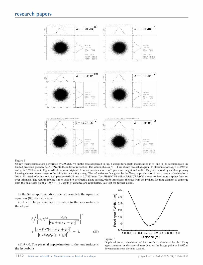
Fig. 5 displays a series of SHADOW3 ray-tracing simula-

tions (Sanchez del Rio et al., 2011) of the lens surfaces

determined by using the X-ray approximation for the six cases

in Fig. 4. All of the 500000 rays originate from a two-dimen-

sional Gaussian source of 1 mm height and width. This is much

smaller than a normal synchrotron electron beam source, but

was chosen to keep down aberrations that appear when the

source size becomes comparable with the lens aperture. The

rays are randomly sampled in angle over a uniform distribu-

tion of horizontal width 1.6 mrad and vertical width 1.6 mrad.

These widths were chosen in order to just exactly cover the full

aperture of the lens surface. Two optical elements are used in

each simulation. The first optical element is used solely to turn

the divergent rays from the source point into a convergent

beam. It is a perfectly reflecting, ideally shaped ellipsoidal

mirror located 23.10287 m from the source point. This mirror

is set to a central grazing incidence angle of 3 mrad. It is

shaped so that its source point coincides with the original

source of the rays and its image point lies 23.10287 m down-

stream. The second optical element is the lens surface. It is

located 0.010 m downstream from the first optical element.

The image point lies 8.6912 m downstream. The basic shape

is a plane surface of aperture 0.07425 mm horizontal �

0.07425 mm vertical. To this plane is added a spline inter-

polation generated by the SHADOW3 utility PRESURFACE

from a 501� 501 mesh of points calculated by MATLAB from

the X-ray approximation of this section. The index of refrac-

tion is taken as constant in the medium upstream from the lens

surface and in the medium downstream from the lens surface.

Absorption is neglected in both media. The displayed plots are

all taken at the final focal point. In all six simulations, the

research papers


distribution of rays in the image fits well to Gaussians of

FWHM very close to 0.886 mm, the geometrical demagnified

source size, in both height and width. A calculation of the spot

size using the SHADOW3 utility RAY_PROP on 17 frames

over a range within �0.8 m from the image point at 8.6912 m

showed that this point was indeed, as required, the point at

which the rays converged (see Fig. 6). It is therefore demon-

strated that the X-ray approximation can indeed generate lens

surfaces that focus convergent beam.

2.4. The paraxial approximation to a conic section

If the incident rays deviate from the central line x = 0 by

only a small amount, the calculations of the ideal lens surface

and of the lens surface in the X-ray approximation both show

that the value yðxÞ of the lens surface will also be small. In this

case, one can assume that the cubic term in equation (47) is

much smaller than the quadratic term, thus leading to the

condition

C3

C2

"yð Þ

�� 1; ð77Þ

for which the cubic term in equation (47) can be neglected.

[Recall that " = 1� ðn0=nÞ2 and that C2 and C3 are defined in

equations (50) and (52), respectively.] In the X-ray approx-

imation, equation (77) reduces to the simple condition

y��

q1 þ q2

� 1: ð78Þ

If equation (77) (for the general case) or equation (78) (for the

X-ray approximation) is fulfilled, then the paraxial approx-

imation is valid. Equation (47) then reduces to

"xð Þ2 ’ C1 "yð Þ þ C2 "yð Þ2; ð79Þ

and equation (57) for the X-ray approximation reduces to

q1 þ q2ð Þy2 þ q1q2ð Þyþq1 � q2ð Þ

2�x2 ¼ 0: ð80Þ

The solutions yðxÞ of these equations are conic sections. The

type of conic section depends on the sign of the quadratic term

y2. Beginning with general values of n0=n, one can complete

the square of equation (79) for two cases:

(i) C2 < 0. The paraxial approximation to the ideal lens

surface is the ellipse

x2

C1= 2ffiffiffiffiffiffiffiffiffiC2

�� q"

� �h i2þ

y� C1= 2 C2

�� " �� 2

C1= 2 C2

�� " �� 2¼ 1: ð81Þ

(ii) C2 > 0. The paraxial approximation to the ideal lens

surface is the hyperbola

yþ C1= 2C2"ð Þ� �2

C1= 2C2"ð Þ� �2 �

x2

C1= 2ffiffiffiffiffiC2

p"

�� 2 ¼ 1: ð82Þ

research papers


Figure 4Examples of solutions of the cubic X-ray approximation [equation (57)] at various values of � for a representative set of values for q1 (23.0929 m) andq2 (8.6912 m). The solutions of the cubic approximation are labelled yðxÞ. The solutions ‘xðyÞ’ were calculated by solving equation (18) as a quadraticequation in x2 with y-dependent coefficients [see equation (45)]. The top row demonstrates three cases in which �> 0 and the bottom row demonstratesthree cases in which �< 0. In each row, �! 0 from left to right. Note the loss of numerical precision in the solutions of the exact formula as j�j decreases,even while the cubic approximation remains numerically stable.

In the X-ray approximation, one can complete the square of

equation (80) for two cases:

(i) �> 0. The paraxial approximation to the lens surface is

the ellipse

x2.(ð�=2Þ1=2 q1q2

q1 þ q2ð Þ q1 � q2ð Þ� �1=2

)2

þyþ ð1=2Þq1q2= q1 þ q2ð Þ� �2

ð1=2Þq1q2= q1 þ q2ð Þ� �2

¼ 1: ð83Þ

(ii) �< 0. The paraxial approximation to the lens surface is

the hyperbola

research papers


Figure 5Six ray-tracing simulations performed by SHADOW3 on the cases displayed in Fig. 4, except for a slight modification in (e) and ( f ) to accommodate thelimited precision given by SHADOW3 to the index of refraction. The values of � = n0=n� 1 are shown on each diagram. In all simulations, q1 is 23.0929 mand q2 is 8.6912 m as in Fig. 4. All of the rays originate from a Gaussian source of 1 mm r.m.s. height and width. They are caused by an ideal primaryfocusing element to converge to the initial focus x = 0, y = �q1. The refractive surface given by the X-ray approximation in each case is calculated on a501 � 501 mesh of points over an aperture 0.07425 mm � 0.07425 mm. The SHADOW3 utility PRESURFACE is used to determine a spline functionover this mesh. The resulting spline is then added to a refractive plane surface, which thus causes the rays from the primary focusing element to convergeonto the final focal point x = 0, y = �q2. Units of distance are centimetres. See text for further details.

Figure 6Depth of focus calculation of lens surface calculated by the X-rayapproximation. A distance of zero denotes the image point at 8.6912 mdownstream from the lens surface.

yþ ð1=2Þq1q2= q1 þ q2ð Þ� �2

ð1=2Þq1q2= q1 þ q2ð Þ� �2

� x2.(ðj�j=2Þ1=2 q1q2

q1 þ q2ð Þ q1 � q2ð Þ� �1=2

)2

¼ 1: ð84Þ

In the limit q1 !þ1 and j�j � 1, equations (83) and (84)

approach the conic sections calculated by Sanchez del Rio &

Alianelli (2012).

An even stricter paraxial approximation is obtained if, in

addition to the condition given in equations (77) or (78), one

demands that the quadratic y2 term in equations (79) or (80)

be much smaller than the linear y term. For general n0=n, this

imposes the additional requirement

C2

C1

"yð Þ

�� 1; ð85Þ

which in the X-ray approximation becomes

q1 þ q2

q1q2

y�� 1: ð86Þ

[One can see that equation (86) is in

fact more stringent than equation (78)

by showing that 1=ðq1 þ q2Þ <

ðq1 þ q2Þ=q1q2 for positive q1 and q2.] If

the conditions of equations (85) or (86)

are fulfilled, the lens surface may be

approximated as a parabola. For general

n0=n, the lens surface is then approxi-

mately

"

C1

x2¼ y; ð87Þ

and in the X-ray approximation the lens

surface is approximately

�1

2�

q1 � q2ð Þ

q1q2

x2¼ �

x2

2�F¼ y; ð88Þ

where F is the geometrical focal length.

Double differentiation of equation (88)

yields the well known relationship

between the radius R and the focal

length F of a single lens surface in the

X-ray approximation, F = R=�.

3. Testing the paraxialapproximation

Figs. 7 and 8 demonstrate how, in the

paraxial approximation, the best conic

section (ellipse for �> 0, hyperbola for

�< 0) and the best parabola deviate

from the X-ray approximation to the

ideal Cartesian oval for � =

� 3:23� 10�6, the value for diamond at

15 keV. Surfaces 2, 24 and 48 were

selected from Table 1 to demonstrate

that the conic section approximations fail at decreasing aper-

tures as the curvature of the surface increases. As mentioned

by previous authors, the parabola deviates from the X-ray

approximation at much smaller apertures than does the best

ellipse or hyperbola. Each plot’s horizontal axis is scaled to

make visible the aperture at which even the best ellipse or

hyperbola begins to deviate from the X-ray approximation.

Thus, for surface 2, which has an aperture of 74.25 mm, one

would expect the parabolic approximation to be sufficient

because it matches the X-ray approximation well out to jxj <

2500 mm. For surface 24, which has an aperture of 59.52 mm,

the parabolic approximation could still be sufficient, but, as

the parabola only matches the X-ray approximation out to

jxj < 200 mm, one might prefer to give this surface an elliptical

or hyperbolic shape. For surface 48, which has an aperture

of 46.760 mm, even the elliptical/hyperbolic approximation

begins to fail at the edges; therefore, this surface must follow

the ideal curve. As a result, surface 48 was chosen for the

research papers


Figure 7In all plots, � = þ3:23� 10�6. The label ‘Cubic’ means that the X-ray approximation of the idealCartesian oval was used to calculate the curve. Refer to Table 1 for the list of surfaces. (a, c, e)Comparison of cubic curve to paraxial ellipse and parabola of surfaces 2, 24 and 48, respectively.(b, d, f ) Deviation of paraxial ellipse and parabola from cubic curve of surfaces 2, 24 and 48,respectively. Solid circles at the ends of a curve indicate that the curve terminates there because theslope dy=dx diverges.

SHADOW ray traces of Fig. 9. To emphasize the improvement

offered by the X-ray approximation over the ellipse/hyper-

bola, the aperture of surface 48 was slightly widened to

63.600 mm, at which Figs. 7 and 8 show that the ellipse or

hyperbola fails severely at the edges. A value � = � 3:2� 10�6

was chosen because of the limited precision given to the index

of refraction input in SHADOW. In each simulation, 500000

rays were randomly selected from a Gaussian source of root

mean square width 0.1 mm (FWHM 0.23548 mm) and uniform

angular distribution. Although the chosen size of the source is

much smaller than the electron beam sizes of real synchrotron

storage rings, it is applied here to approximate a true point

source, eliminating aberrations that would appear in the focal

spot if the source size were comparable with the lens surface’s

aperture. Two optical elements were created. The first was a

purely theoretical spherical mirror designed to reflect all rays

from the source at normal incidence. This element exists only

to produce the necessary convergent beam for the second

element, which is the lens surface itself. The second element is

situated 12.227 mm upstream from the focus of the spherical

mirror. It is simulated with a plane

figure to which a spline file generated by

the SHADOW utility PRESURFACE is

added. MATLAB was used to calculate

a cylinder for one-dimensional focusing

with 501 points over a width of

46.760 mm in the non-focusing direction

and 681 points over a width of

63.600 mm in the focusing direction. The

rays in the calculated profiles were

sorted into 250 bins according to their

position. Figs. 9(a) and 9(c) show the

beam profiles generated at the nominal

focus 10.999 mm downstream from

surface 48, comparing them with the

original source. The profiles generated

by the ellipse or hyperbola are slightly

but noticeably lower at the peak and

have slightly larger tails than those

generated by the X-ray approximation

to the ideal curve. The profiles gener-

ated by the parabola show a loss of

about 50% of the peak intensity and

correspondingly severe tails. Depth of

focus plots showing the variation of the

beam size versus the distance along the

beam direction from the nominal focus

were generated by the SHADOW3

utility RAY_PROP and are displayed in

Figs. 9(b) and 9(d). The X-ray approx-

imation yields a lens surface that mini-

mizes the beam width at the nominal

focus, as required. The FWHM of the

beam profile at this minimum is

0.210 mm, which matches the geome-

trically demagnified source size. The

ellipse/hyperbola shifts the minimum of

the beam width closer to the lens surface by 10–20 mm, and

this minimum is still not quite as small as that achieved by the

X-ray approximation. The parabola shifts the minimum of

the beam width by about 60–70 mm from the nominal focus,

and this minimum is considerably larger than that achieved

by either the X-ray approximation or the ellipse/hyperbola.

These results again demonstrate that the X-ray approximation

can generate lens surfaces that focus convergent beam better

than the approximate conic sections can do.

4. Diffraction broadening

SHADOW was used to calculate the effective aperture of the

CRL in Table 1. 500000 rays of 15 keV energy were created

from a point source. They were uniformly distributed in angle

so that the entire geometrical aperture of the first lens surface

(0.075 mm � 0.075 mm) was illuminated. Each lens surface

was assumed to be a parabolic cylinder, focusing in the vertical

direction only. All of the lens surfaces except the first were

taken to be unbounded so that their limited geometrical

research papers


Figure 8In all plots, � = �3:23� 10�6. The label ‘Cubic’ means that the X-ray approximation of the idealCartesian oval was used to calculate the curve. Refer to Table 1 for the list of surfaces. (a, c, e)Comparison of cubic curve to paraxial hyperbola and parabola of surfaces 2, 24 and 48, respectively.(b, d, f ) Deviation of paraxial hyperbola and parabola from cubic curve of surfaces 2, 24 and 48,respectively.

apertures would not cut off any of the rays propagating inside

the CRL. The lens material is diamond, which for 15 keV

X-rays has an index of refraction differing from 1 in its real

part by �3.23 � 10�6. The linear absorption coefficient � is

0.282629 mm�1. The calculated intensity distribution on the

last surface (number 48) and the calculated angular distribu-

tion of the intensity converging onto the final focus are

displayed in Figs. 10(a) and 10(b), respectively. The effective

aperture is the FWHM of the plot in Fig. 10(a), 26.47 mm. The

corresponding numerical aperture is half the FWHM of the

angular plot in Fig. 10(b), 1.204 mrad.

The diffraction broadening therefore

amounts to 0.75�/(2NA) = 25.74 nm,

which is much less than the focal spot

widths in Fig. 9. Moreover, within the

FWHM effective aperture in Fig. 10(a),

a parabola is still a sufficiently good

approximation to the ideal shape of the

final lens surface, as shown in Figs. 7(e)

and 7( f).

5. Conclusions

The immediate goal of this paper was

to prove that an analytical solution,

namely a Cartesian oval, exists for a lens

surface that is to refocus an incident

beam converging to a point into a new

beam converging to a point closer to

the lens surface. This result serves the

long-term goal of designing aberra-

tion-free aspherical CRLs that will in

future produce X-ray beam spots of

50 nm width and, further on, even

10 nm width. Numerical difficulties

that arose in the analytical calculation

of the Cartesian oval when the change

in refractive index across the lens

surface is small, as is usual for X-ray

optics, were overcome by a cubic

approximation that was numerically

stable. The focusing performance of

lens surfaces following the cubic

‘X-ray’ approximation was compared

with that of lens surfaces shaped either

as ellipses or hyperbolas, or as para-

bolas, as previous authors have

suggested. Elliptical or hyperbolic lens

surfaces yield stronger peaks and

lower tails at the focus than do para-

bolic lens surfaces, but surfaces that

follow the cubic X-ray approximation

provide better focal profiles than

either. Examples taken from a

proposed adiabatically focusing lens,

in which the radius of curvature and

the aperture of the lens surfaces both

decrease along the beam direction, indicate that the advan-

tages of the X-ray approximation over conic sections are most

apparent in the final, most strongly curved, lenses.

Acknowledgements

L. A. would like to thank M. Sanchez del Rio (ESRF) for the

many illuminating discussions on optics and on numerical

methods in SHADOW.

research papers


Figure 9SHADOW ray-tracing calculations using surface 48 of Table 1 over a geometrical aperture Ax of63.600 mm. The source is a Gaussian with a root mean square width of 0.1 mm. (a, c) Profiles of sourceand of focal spots produced by the cubic curve, the paraxial conic section (ellipse/hyperbola) and theparabola for � =þ3:2� 10�6 and � =�3:2� 10�6, respectively. (b, d) FWHM of focal spots producedby the cubic curve, the paraxial conic section (ellipse/hyperbola) and the parabola for � =þ3:2� 10�6

and � = �3:2� 10�6, respectively, as a function of distance along the beam from the nominal focus.See text for details.

Figure 10(a) Vertical intensity distribution calculated by SHADOW ray trace on final lens surface (number48) of the CRL in Table 1. (b) Vertical angular distribution of intensity calculated by SHADOW raytrace at the final focus of the CRL of Table 1. Each histogram sorts the 500000 rays of the simulationinto 200 bins. See text for details.

research papers


References

Alianelli, L., Laundy, D., Alcock, S., Sutter, J. & Sawhney, K. (2016).Synchrotron Radiat. News, 29(4), 3–9.

Alianelli, L., Sanchez del Rio, M., Fox, O. J. L. & Korwin-Mikke, K.(2015). Opt. Lett. 40, 5586–5589.

Alianelli, L., Sawhney, K. J. S., Barrett, R., Pape, I., Malik, A. &Wilson, M. C. (2011). Opt. Express, 19, 11120–11127.

Aristov, V., Grigoriev, M., Kuznetsov, S., Shabelnikov, L., Yunkin, V.,Weitkamp, T., Rau, C., Snigireva, I., Snigirev, A., Hoffmann, M. &Voges, E. (2000). Appl. Phys. Lett. 77, 4058–4060.

Evans-Lutterodt, K., Ablett, J. M., Stein, A., Kao, C.-C., Tennant,D. M., Klemens, F., Taylor, A., Jacobsen, C., Gammel, P. L.,Huggins, H., Ustin, S., Bogart, G. & Ocola, L. (2003). Opt. Express,11, 919–926.

Evans-Lutterodt, K., Stein, A., Ablett, J. M., Bozovic, N., Taylor, A. &Tennant, D. M. (2007). Phys. Rev. Lett. 99, 134801.

Fox, O. J. L., Alianelli, L., Malik, A. M., Pape, I., May, P. W. &Sawhney, K. J. S. (2014). Opt. Express, 22, 7657–7668.

Kohn, V. G. (2017). J. Synchrotron Rad. 24, 609–614.Lengeler, B., Schroer, C., Tummler, J., Benner, B., Richwin, M.,

Snigirev, A., Snigireva, I. & Drakopoulos, M. (1999). J. SynchrotronRad. 6, 1153–1167.

Lengeler, B., Tummler, J., Snigirev, A., Snigireva, I. & Raven, C.(1998). J. Appl. Phys. 84, 5855–5861.

MathWorks (2004). MATLAB Version 7.0.1.24704 (R14) ServicePack 1. MathWorks, Inc., Natick, Massachusetts, USA.

Nohammer, B., Hoszowska, J., Freund, A. K. & David, C. (2003).J. Synchrotron Rad. 10, 168–171.

Sanchez del Rio, M. & Alianelli, L. (2012). J. Synchrotron Rad. 19,366–374.

Sanchez del Rio, M., Canestrari, N., Jiang, F. & Cerrina, F. (2011).J. Synchrotron Rad. 18, 708–716.

Schroer, C. G. & Lengeler, B. (2005). Phys. Rev. Lett. 94, 054802.Snigirev, A., Kohn, V., Snigireva, I. & Lengeler, B. (1996). Nature

(London), 384, 49–51.Suzuki, Y. (2004). Jpn. J. Appl. Phys. 43, 7311–7314.Weisstein, E. W. (2016). MathWorld – A Wolfram Web Resource,

http://mathworld.wolfram.com.

http://scripts.iucr.org/cgi-bin/cr.cgi?rm=pdfbb&cnor=yi5037&bbid=BB1





































Documents

Aberration-free aspherical lens shape for shortening the