Abiotic and biotic resources impact categories in LCA

Abiotic and biotic resources impact categories in LCA: development of new approaches

Accounting for abiotic

resources dissipation

and biotic resources

Beylot A., Ardente F., Marques A., Mathieux F., Pant R., Sala S., Zampori L.

2020

EUR 30126 EN

This publication is a Technical report by the Joint Research Centre (JRC), the European Commission’s science and

knowledge service. It aims to provide evidence-based scientific support to the European policymaking process.

The scientific output expressed does not imply a policy position of the European Commission. Neither the

European Commission nor any person acting on behalf of the Commission is responsible for the use that might

be made of this publication. For information on the methodology and quality underlying the data used in this

publication for which the source is neither Eurostat nor other Commission services, users should contact the

referenced source. The designations employed and the presentation of material on the maps do not imply the

expression of any opinion whatsoever on the part of the European Union concerning the legal status of any

country, territory, city or area or of its authorities, or concerning the delimitation of its frontiers or boundaries.

Contact information

Name: Serenella Sala

Address: Via E. Fermi, 2749 21027, Ispra (VA) Italy

Email: [email protected]

Tel.: +39 0332786417

EU Science Hub

https://ec.europa.eu/jrc

JRC120170

EUR 30126 EN

PDF ISBN 978-92-76-17227-7 ISSN 1831-9424 doi:10.2760/232839

Print ISBN 978-92-76-17228-4 ISSN 1018-5593 doi:10.2760/815673

Luxembourg: Publications Office of the European Union, 2020

© European Union 2020

The reuse policy of the European Commission is implemented by the Commission Decision 2011/833/EU of 12

December 2011 on the reuse of Commission documents (OJ L 330, 14.12.2011, p. 39). Except otherwise noted,

the reuse of this document is authorised under the Creative Commons Attribution 4.0 International (CC BY 4.0)

licence (https://creativecommons.org/licenses/by/4.0/). This means that reuse is allowed provided appropriate

credit is given and any changes are indicated. For any use or reproduction of photos or other material that is not

owned by the EU, permission must be sought directly from the copyright holders.

All content © European Union 2020, except: cover image – copper wire, © salita2010 - stock.adobe.com; cover

image – fish in ocean, © kichigin19 - stock.adobe.com

How to cite this report: Beylot, A., Ardente, F., Penedo De Sousa Marques, A., Mathieux, F., Pant, R., Sala, S.

and Zampori, L., Abiotic and biotic resources impact categories in LCA: development of new approaches, EUR

30126 EN, Publications Office of the European Union, Luxembourg, 2020, ISBN 978-92-76-17227-7,

doi:10.2760/232839, JRC120170.

https://creativecommons.org/licenses/by/4.0/

i

Contents

Acknowledgements ............................................................................................................................................................................................................................... 1

Abstract .................................................................................................................................................................................................................................................................. 2

1 Introduction............................................................................................................................................................................................................................................. 3

1.1 Policy context .................................................................................................................................................................................................................................. 3

1.2 Abiotic and biotic resources in the Environmental Footprint ............................................................................................................. 4

1.2.1.1 Mineral and metal resource use.................................................................................................................................................... 4

1.2.1.2 Biotic resource use ..................................................................................................................................................................................... 5

1.3 Overall approach undertaken in the project and report outline ..................................................................................................... 5

2 Resource dissipation: a definition building from the literature ............................................................................... 6

2.1 On the concept of resources............................................................................................................................................................................................. 6

2.2 On the concept of resource dissipation ................................................................................................................................................................. 7

2.3 Abiotic resource dissipation: a definition .............................................................................................................................................................. 8

2.4 Biotic resource dissipation: a definition ................................................................................................................................................................. 9

3 Evaluation of existing approaches to assess resource dissipation .................................................................. 10

3.1 Approaches available in the literature: short description .................................................................................................................. 10

3.2 Aspects considered in the evaluation of approaches ............................................................................................................................ 10

3.3 Results of the evaluation, by approach............................................................................................................................................................... 11

3.3.1 “Abiotic resource dilution (ARD)” .............................................................................................................................................................. 12

3.3.2 “Ultimate quality limit” and “backup technology” concepts........................................................................................... 13

3.3.3 “Relative Statistical Entropy (RSE)” ....................................................................................................................................................... 14

3.4 Conclusion on the evaluation of existing approaches ........................................................................................................................... 15

4 Suggested approach to account for mineral and metal resource dissipation in Life Cycle Inventories .................................................................................................................................................................................................................................. 16

4.1 Definition of “mineral and metal resources”.................................................................................................................................................. 16

4.1.1 “Mineral and metal resources” in current LCI practices .................................................................................................... 16

4.1.2 “Mineral and metal resources” in the context of resource dissipation: a proposal ................................. 16

4.2 Dissipative flows at the unit process level ...................................................................................................................................................... 17

4.2.1 Rationale of the approach ............................................................................................................................................................................. 17

4.2.2 List of flows to be considered “dissipative” in LCI datasets ......................................................................................... 20

4.2.3 Discussion on potential specific cases regarding dissipative flows ...................................................................... 21

4.3 Comments on potential implementation for LCI datasets construction ............................................................................. 22

5 Suggested approach for impact assessment of mineral and metal resources ............................. 24

5.1 A price-based approach ..................................................................................................................................................................................................... 24

5.2 Impact Assessment and characterisation factors .................................................................................................................................... 24

5.2.1 Data quality and availability ....................................................................................................................................................................... 24

5.2.2 Calculation of the characterisation factors .................................................................................................................................. 25

ii

5.3 Normalisation factors .......................................................................................................................................................................................................... 27

6 Application to case studies ........................................................................................................................................................................................... 31

6.1 Case study 1: Cradle-to-gate production of primary copper .......................................................................................................... 31

6.1.1 System boundaries ............................................................................................................................................................................................... 31

6.1.2 Life Cycle Inventory phase ............................................................................................................................................................................ 32

6.1.2.1 Overall approach for inventory compilation ................................................................................................................... 32

6.1.2.2 Mining and concentration ................................................................................................................................................................. 33

6.1.2.3 Pyrometallurgy ............................................................................................................................................................................................ 35

6.1.2.4 Cradle to gate inventory .................................................................................................................................................................... 37

6.1.3 Life Cycle Impact Assessment ................................................................................................................................................................... 38

6.1.4 Comparison with alternatives for inventory and impact assessment ................................................................. 39

6.1.4.1 Inventory of dissipative flows in a long-term perspective ............................................................................... 39

6.1.4.2 Inventory and impact assessment using a depletion approach .................................................................. 39

6.2 Case study 2: Life cycle of flame-retarded PVC electrical cable ............................................................................................... 40

6.2.1 System boundaries ............................................................................................................................................................................................... 41

6.2.1.1 Polyvinyl Chloride ..................................................................................................................................................................................... 42

6.2.1.2 Additives: flame retardants, fillers, plasticizers .......................................................................................................... 42

6.2.1.3 Copper content ............................................................................................................................................................................................ 42

6.2.1.4 End of life treatment of PVC cables ....................................................................................................................................... 42

6.2.2 Life Cycle Inventory ............................................................................................................................................................................................. 43

6.2.3 Life Cycle Impact Assessment ................................................................................................................................................................... 45

7 Suggested approach for the impact assessment of biotic resources .......................................................... 48

7.1 State of the art of naturally occurring biotic resources in LCA.................................................................................................... 48

7.2 Characterisation models for the impact assessment of natural biotic resources ..................................................... 49

7.2.1 Elementary flows of natural occurring biotic resources (NOBR) .............................................................................. 49

7.2.2 Renewability indicator ....................................................................................................................................................................................... 50

7.2.3 Exploitation scores ................................................................................................................................................................................................ 51

7.2.3.1 Fish ......................................................................................................................................................................................................................... 51

7.2.3.2 Forest ................................................................................................................................................................................................................... 52

7.2.3.3 Other wild species .................................................................................................................................................................................... 52

7.2.4 Vulnerability scores .............................................................................................................................................................................................. 52

7.2.5 Characterization of NOBR taking into account renewability and level of exploitation ....................... 53

7.2.5.1 Option 1 ............................................................................................................................................................................................................. 54

7.2.5.2 Option 2 ............................................................................................................................................................................................................. 55

7.2.5.3 Option 3 ............................................................................................................................................................................................................. 56

7.2.5.4 Option 4 ............................................................................................................................................................................................................. 57

7.3 Operationalizing the impact assessment of natural biotic resources: fish case study ......................................... 58

iii

7.3.1 Characterization factors for fish species taking into account renewability and exploitation level. 58

7.3.2 Impacts of EU’s fish consumption ......................................................................................................................................................... 60

8 Conclusions ........................................................................................................................................................................................................................................... 63

References ....................................................................................................................................................................................................................................................... 65

List of abbreviations and definitions ....................................................................................................................................................................... 72

List of figures .............................................................................................................................................................................................................................................. 74

List of tables ................................................................................................................................................................................................................................................. 75

Annexes ............................................................................................................................................................................................................................................................... 76

Annex 1. Definitions for natural resources .......................................................................................................................................... 76

Annex 2. The concept of resource dissipation in the literature: list of publications reviewed .................................................................................................................................................................................................................................................... 79

Annex 3. Coefficient of variation for the prices of different resources ..................................................... 82

Annex 4. Proposal of elementary flows for natural occurring biotic resources (International Life Cycle Data system – compliant) .............................................................................................................. 83

Annex 5. Renewability indicators for naturally occurring biotic resources ......................................... 85

Annex 6. Characterization factors for NOBR fish........................................................................................................................ 89

Annex 7. Characterization factors for product groups ....................................................................................................... 90

1

Acknowledgements

The authors would like to acknowledge the financial support of the Directorate General for

the Environment (DG ENV) in the framework of the Administrative Arrangement on Support

for Environmental Footprint and Life Cycle Data Network (EFME3)

(07.0201/2015/704456/SER/ENV.AI).

Moreover, the authors would like to thank Simone Fazio and Gian Andrea Blengini for their

helpful comments along the project development.

The contribution of the participants to the workshop organised in Brussels on December

12th 2019 are also acknowledged.

Authors

Antoine Beylot: Chapter 1, 2, 3, 4, 5, 6, 8

Fulvio Ardente: Chapter 1, 2, 3, 4, 5, 6, 8

Alexandra Marques: Section 2.4 of Chapter 2 and Chapter 7

Fabrice Mathieux: overall review of the parts on abiotic resources

Rana Pant: project coordinator until December 2019

Serenella Sala: overall review, Chapter 7, project coordinator from December 2019

Luca Zampori: Chapter 1, 2, 3, 4, 5, 6, 8

2

Abstract

Depletion is the concept underpinning one of the most widely applied approach to account

for the impacts associated with mineral and metal resource use in Life Cycle Impact

Assessment (LCIA) step.

The extraction of a resource from the Earth’s crust implies the reduction of the

corresponding geological stocks, and is considered to subsequently contribute to this

resource depletion.

During the Environmental Footprint (EF) pilot phase (2013-2018), the concept of resources

(or materials) dissipation after their use in the technosphere has been increasingly called

for being considered as a potential better way to account for (abiotic) resources in an EF

context. The international community has started investigating further the concept of

resource dissipation applied to Life Cycle Assessment (LCA) and, still, there is currently no

common understanding of what a dissipative flow is, if this has implications on how to

define the Life Cycle Inventory (LCI) of a process, nor there is an accepted LCIA model to

be applied to dissipative flows.

This report provides a literature review of existing studies in different disciplines regarding

resource dissipation. Furthermore, it provides an approach on how to deal with resource

dissipation at the LCI and LCIA levels. The proposed approaches were tested in case

studies.

Moreover, the report addresses another aspects so far not properly developed in LCIA: the

impact associated to the use of naturally occurring biotic resources and a proposal for the

characterization thereof.

The results of this study cannot be integrated “as is” in an EF context: when considering

abiotic and biotic resources still some further work is needed both at LCI and LCIA levels.

However, for what concerns biotic resources, a list of elementary flows that can be

integrated in EF is provided. Nevertheless, this work constitutes the basis for further

developments by researchers and method developers for a possible consideration for

implementation in an EF context. As a next step we invite the scientific community to build

on the results of this report in view of a fully applicable method.

3

1 Introduction

1.1 Policy context

In 2011, the Joint Research Centre of the European Commission (EC-JRC) published the

International Reference Life Cycle Data System (ILCD) Handbook recommendations on the

use of Impact Assessment models for use in Life Cycle Assessment (LCA; EC-JRC, 2011).

This created the basis for the Product and Organisation Environmental Footprint (PEF/OEF)

recommendations for impact categories and models as per Recommendation 2013/179/EU

on the use of common methods to measure and communicate the life cycle environmental

performance of products and organisations (EC, 2013a). This Recommendation is expected

to contribute to Building the Single Market for Green Products (EC, 2013b) by supporting

a level playing field regarding the measurement of environmental performance of products

and organisations. “Life cycle environmental performance” is defined as a “quantified

measurement of the potential environmental performance taking all relevant life cycle

stages of a product or organisation into account, from a supply chain perspective”. The

Recommendation 2013/179/EU accordingly follows the ISO 14040 series which states that

LCA addresses the environmental aspects and potential environmental impacts (e.g. use

of resources and the environmental consequences of releases) throughout a product's life

cycle. In the period 2013-2018, the PEF pilot phase enabled the development of Product

Environmental Footprint Category Rules (PEFCRs) and of approaches on how to verify and

communicate the resulting information to different stakeholders. Volunteering industries

led this work under the supervision and with the input of different European Commission

services, Member States, EU and international stakeholders. Several methodological topics

have been further developed through this multi-stakeholder process, making the method

stronger, more reliable and more implementable. In 2019, the Joint Research Centre

published suggestions on how the PEF method should be amended in the future to reflect

the developments and the practical experience gained during the pilot phase (Zampori and

Pant, 2019).

During the PEF pilot phase, the need of updating the impact assessment models used in

the EF method emerged. Hence, a number of impact categories have been revised, leading

to publication of specific updates for toxicity-related categories (Saouter et al., 2019) and

on land use, water use, particulate matter and resources (Sala et al., 2019). In these

updates, compared to the original EF recommendation in 2013, resources were split in two

categories (mineral and metals, and fossil) and the impact assessment model adopted has

been the abiotic depletion potential, ultimate reserve.

However, traditional approaches to resource assessment in LCA has been the object of

ample debate, both at the inventory and impact assessment level, e.g. to respond to

specific societal and policy perspectives. At policy level, since the publication of the Raw

Material Initiative in 2008 (EC, 2008), there has been a growing focus on sustainable

supply of raw materials from EU sourcing and from global markets but also on resource

efficiency and recycling. More recently, the EU action plan for the circular economy fostered

the transition towards a more circular economy, in which “the value of products, materials

and resources is maintained […] for as long as possible, and the generation of waste

minimised” as an essential contribution “to develop a sustainable, low carbon, resource

efficient and competitive economy” (EC, 2015). “Circular economy” is an economy in which

the instrumental value/function of the natural resources (extracted, harvested and overall

transformed) are maintained for the beneficial use by humans, for as long as possible. This

is not an economy that maximises recycling of all elements no matter what the cost. Still,

recalling that “sustainable development” is the “development that meets the needs of the

present without compromising the ability of future generations to meet their own needs”,

circular economy practices and related business models should preserve resources for

current and future generations, and can help to achieve several of the Sustainable

Development Goal targets (Schroeder et al., 2019). Attention should be shifted from the

extraction of natural resources to the way they are used and how their use can impact our

society.

4

1.2 Abiotic and biotic resources in the Environmental Footprint

For a PEF study, 16 impact categories (with respective impact category indicators,

characterization models and default characterization factors) shall be applied, without

exclusion (Zampori and Pant, 2019). Two impact categories address resources (“resource

use, minerals and metals”, and “resource use, fossils”), while biotic resources are currently

not taken into account. In this study, we present developments regarding both abiotic and

biotic resources. Abiotic resource indicators are presented and discussed with focus on

mineral and metal resources, and their dissipation. Biotic resource are presented with a

focus on naturally occurring biotic resources, and a proposal for their characterisation.

1.2.1.1 Mineral and metal resource use

One of the most widely applied approaches to account for the impacts associated with

mineral and metal resource use in the Life Cycle Impact Assessment (LCIA) step relies on

the concept of “depletion”: once a resource is extracted from the Earth’s crust, it is

considered depleted. The corresponding ADP (Abiotic Depletion Potential, ultimate reserve;

Guinée et al., 2002; van Oers et al., 2002) model is currently recommended:

- by the European Commission (EC) within the framework of the EF to assess the impacts

due to mineral and metal resource use (Zampori and Pant, 2019);

- by the Task Force “Mineral Resources” (within the “Global Guidance for LCIA Indicators

and Methods” project of the Life Cycle Initiative hosted by UN Environment), with

characterization factors as in CML (2016), when the question under study is: “How can I

quantify the relative contribution of a product system to the depletion of mineral

resources?” (Berger et al., 2020).

However, abiotic resources may remain in the anthropogenic system, although

transformed, and may be available for further uses. Accordingly, several authors

(Yellishetty et al., 2011; Klinglmair et al., 2014; Frischknecht, 2014; Schneider et al., 2011

and 2015; and van Oers and Guinée, 2016) have discussed the possibility to consider also

the amount of resources in the technosphere (as stocks in products) as part of the whole

stock potentially available, and to include them in the calculation of characterization factors

for assessing resource depletion. In parallel, the concept of resources (or materials)

dissipation after their use in the technosphere, opposite to the concept of stocks of

resources potentially available within the technosphere, has been increasingly called for

being considered in LCA (Stewart and Weidema, 2005; Vadenbo et al., 2014, Zampori and

Sala, 2017; Ardente et al., 2019). In particular, Stewart and Weidema (2005) used a

generic concept of the quality state of resources to show that it is not the extraction of

materials which is of concern, but rather the dissipative use and disposal of materials. More

recently, an alternative for a way forward to assess abiotic resources was suggested by

the Technical Secretariat (TS) dealing with the Organisation Environmental Footprint

Sector Rule (OEFSR) for the copper producing sector (EC, 2018a). The possible way

forward is described in Annex V of the OEFSR on copper production (EC, 2018b),

distinguishing two steps: firstly, adapting the Life Cycle Inventories (LCI), and secondly

associating a characterization model to the new built inventories. Zampori and Sala (2017)

focused on the possible applications of the dissipation concept to LCA and described

possible alternatives for structuring life cycle inventories. The dissipation of resources was

identified as a promising concept, whose feasibility for implementation in LCA has been

further discussed (Ardente et al., 2019).

Still, there is currently no common understanding of what a dissipative flow is, no synthesis

on the studies that have used this concept so far (Lifset et al., 2012; Zimmermann, 2017),

and there are still research needs before an approach can be practically implemented to

account for resource dissipation in LCA (Beylot et al., 2020). To operationalize this concept

in LCA, the LCIs need to provide information about dissipative losses or flows, as

complements to the currently reported flows associated with resource extraction, and LCIA

methods should be consistent to account for the impacts associated with these dissipative

flows (Berger et al., 2020). In this context, a number of on-going projects aim at providing

5

a framework to account for resource dissipation (or decrease of accessibility) in LCA (e.g.

Drielsma and Sochorová, 2019; Charpentier Poncelet et al., 2019). When possible, the JRC

has monitored the developments of these recent or on-going projects and their findings

were considered in the preparation of this report.

1.2.1.2 Biotic resource use

Generally, biotic resources are still poorly covered in available LCIA methods (Finnveden

et al., 2009, Crenna et al. 2018). The current EF recommendations do not include

characterization factors for biotic resources (Zampori and Pant, 2019). The need for

improvements and further research for biotic resource proper assessment has emerged

(Sala et al., 2019).

With the growing degradation of ecosystems, including overexploitation related pressures,

(Tittensor et al. 2014, IPBES, 2019) addressing the impacts of the extraction of biotic

resources when assessing environmental sustainability is thus essential. Over the last

years, few attempts of developing new LCIA methods for biotic resources have been made

(e.g. Crenna et al. 2018, Bach et al. 2017, Hélias et al. 2018). Critical aspects to take into

consideration are the renewability/regeneration rate of a certain biotic resource, the

carrying capacity of the ecosystem securing its provision (Klinglmair et al., 2014, Sala et

al, 2013a,b). These will determine the “renewability” of the biotic resource; if the extraction

rate surpasses the renewability/regeneration rate then the carrying capacity of the

ecosystem is overcome and the resource will tend to exhaustion. Moreover, there is an

aspect of vulnerability of the resource to be considered, namely that species already at

risk, even with a short renewability time, may go to extinction (hampering the biotic

provision of the resource itself).

1.3 Overall approach undertaken in the project and report outline

In this context, regarding abiotic resources, this report describes an approach developed

by the JRC in 2018-2019 to account for the impact associated with resource dissipation

along the life cycle of a product or a system, taking into account its applicability in the

context of the EF. The following approach has been considered in the project:

- Analysis of policy needs;

- Analysis of scientific literature and on-going initiatives;

- Development of a concept;

- Test of the concept on two case studies;

- Consultation of stakeholders through a workshop (on the 12th December 2019 in

Brussels);

- Preparation of the final report and related scientific articles.

The report first discusses the concept of resource dissipation, building from a literature

review on life-cycle based studies (Section 2). Moreover, existing approaches to potentially

assess resource dissipation in an EF context are evaluated (Section 3), before the proposed

approach to account for mineral and metal resource dissipation is presented: the Life Cycle

Inventory (Section 4) and possible method(s) for the impact assessment (Section 5) are

distinguished. This approach is applied and discussed considering two case studies,

concerning cradle-to-gate production of primary copper and production and life cycle of

flame-retarded PVC electric cable (Section 6), Conclusions and perspectives are finally

formulated (in Section 8).

For biotic resources, we briefly discuss the concept of biotic resource dissipation (Section

2), however the rest of the work is focused on improving, from a methodological point of

view, the impact assessment of biotic resource exploitation (Section 7).

6

2 Resource dissipation: a definition building from the

literature

The concept of resources or materials dissipation after their use in the technosphere has

been increasingly considered in studies based on Substance Flow Analysis (SFA), Material

Flow Analysis (MFA), Input-Output Analysis (IOA), and LCA. This section firstly presents a

discussion on the concepts of resources and resource dissipation, building from the

literature. Moreover, from the different understandings of the concept of “resource

dissipation” as found in the literature, it provides one definition that is considered further

in the development of an approach (proposed in Section 4) to account for resource

dissipation in LCA.

2.1 On the concept of resources

In their discussion on mineral resources in LCIA, Drielsma et al. (2016) recall the traditional

definitions utilized by leading geological institutions, underlining the critical need for

appropriate definitions when models are constructed. Similarly in this report, it appears

essential to first elaborate on the concept of natural resources before the concept of

resource dissipation can be appropriately discussed.

The ISO 14040-44 (2006), which sets the principles and framework for LCA, does not

provide any definition for the term “resources”, while stating that “LCA addresses the

environmental aspects and potential environmental impacts (e.g. use of resources […])

throughout a product's life cycle”. More recently, Sonderegger et al. (2017) defined natural

resources as “material and non-material assets occurring in nature that are at some point

in time deemed useful for humans”. The International Resource Panel referred to resources

(“including land, water, air and materials”) as “seen as parts of the natural world that can

be used in economic activities to produce goods and services” (IRP, 2019). Overall,

considering a (non-exhaustive) list of definitions (as provided in environmental, economic,

social and law studies), Ardente et al. (2019) performed a non-exhaustive overview of

definitions of natural resources as in the literature and identified several key elements

usually conveyed by different authors when defining or, more generally, referring to

“resource(s)” (see some definitions as provided in Annex 1). Despite the heterogeneity of

these definitions (in a context where the scopes of the source publications are also very

heterogeneous), and the different perspectives in the accounting and assessment thereof

(Dewulf 2015a,b), they converge in referring to a “resource” when it has an intrinsic “value”

or “utility” (i.e. by providing a certain function) for a certain subject (generally humans, in

the common anthropogenic perspective). The value or function of resources is not

exclusively “economic”, but can be linked, for example, to the overall human well-being

(e.g. through the “cultural value” of resources). Linking the concept of resources to their

“function” or “utility” for the target subject can be relevant also when estimating potential

resource losses.

Moreover, “mineral resources” have been specifically defined as “chemical elements (e.g.

copper), minerals (e.g. gypsum), and aggregates (e.g. sand) as embedded in a natural or

anthropogenic stock” by the Task Force “Mineral Resources” of the United Nations

Environment and Setac (UNEP-SETAC) “Life Cycle Initiative”1 (Berger et al., 2020:

Sonderegger et al. 2020). It is additionally stated that “within the area of protection

“natural resources”, the safeguard subject for “mineral resources” is the potential to make

use of the value that mineral resources can hold for humans in the technosphere. The

damage is quantified as the reduction or loss of this potential caused by human activity.”

Biotic resources are considered all resources extracted by humankind from nature, but only

if not reproduced by a production process (for example extraction of wood from a forest

plantation does not classify as extraction of a biotic resource) (Guinée and Heijungs, 1995).

Crenna et al. 2018 defined naturally occurring biotic resources (NOBR), as those

1 https://www.lifecycleinitiative.org/

7

commercially valuable resources proceeding from biological sources that are caught or

harvested from the ecosphere.

2.2 On the concept of resource dissipation

More than 20 years after the concept of “resource dissipation” has been first mentioned as

potentially applicable to assess the impact on natural resources in LCA, there is currently

no common understanding of what a dissipative flow is (Lifset et al., 2012; Zimmermann,

2017). In this context, Beylot et al. (2020) reviewed 45 publications presenting results of

life-cycle-based studies (that is, studies that trace the flows of resources from their

extraction to their end-of-life; see Annex 2 for the list of publications reviewed). The review

describes the status of resource dissipation in the literature, discussing how resource

dissipation is usually defined, which temporal perspective is considered, which

compartments of dissipation are distinguished, and which approaches can be used to

assess resource dissipation in a system. Based on the review, it is noteworthy that:

overall, existing life-cycle-based studies dealing with the concept of dissipation

mainly target abiotic resources, and in particular metals. Yet some studies also

apply or discuss the concept of dissipation with respect to biotic resources;

a definition for the concept of “resource dissipation” is given in only 33% of the

cases. When provided, definitions relate the concept of dissipated resources to the

difficulty, or even to the impossibility, to recover or to recycle these resources;

the concept of dissipation is analysed and discussed with predominantly employing

the term “dissipation” and its derivate terms: “dissipated” and “dissipative”.

However, the term “loss” is also used in many publications, in most cases with

directly connecting it to (but not necessarily setting it equivalent to) the concept of

“dissipation”;

in their definitions, or as complements to their definitions, several authors refer to

temporal aspects. In particular, (the impossibility of) future recovery or the

unavailability for future users are mentioned in some definitions. However, in more

than 2/3 of the reviewed publications, no temporal aspect is referred to with respect

to resource dissipation. Moreover, when temporal aspects are referred to (in the

remaining 1/3 of the reviewed publications), no precise time-frame perspective is

set;

most publications account, more or less explicitly, for dissipative flows to (or within)

at least one of the three following compartments:

- air/water/soil (environment), which relates to what is usually called “emissions to the

environment” in MFA and LCA studies. For example, emissions of copper associated with

its use in specific applications (e.g. pesticides, brake pads, etc.) are considered to be

dissipative flows to the environment (Lifset et al., 2012);

- final waste disposal facilities (in technosphere). This in particular corresponds to landfills

and tailings management facilities (e.g. critical metals with a share dissipated to slags

disposed of in landfills; Thiébaud et al., 2018);

- and products in use (in technosphere). The latter includes two main types of flows: a)

dissipation associated with non-functional recycling (i.e. collection of old metal scrap

flowing into a large magnitude material stream, as a “tramp” or impurity elements); and

b) dissipation in products as a driver of subsequent dissipation in the life cycle (through

emissions to the environment during the product use, or through final waste disposal). For

example, Licht et al. (2015) report in their study that the indium used in solders and alloys

is considered as a “dissipative use and unrecoverable” (considered a “dissipation in a

product-in-use” in Beylot et al., 2020), further specifying that “it can be considered

dissipative at the end-of-life”. The impossibility to access the material embodied in a

product in use, due to its more or less long residence time as used in the technosphere, is

considered as a type of dissipation only by a limited number of authors.

8

in order to quantify dissipative flows in the system under study, most authors define

a set of flows that they consider as “dissipative” per se2 and then calculate the

corresponding masses based on different types of data (statistics, process data,

assumptions, etc.). Only a few authors mention parameter-based and threshold-

based approaches to distinguish dissipative flows from non-dissipative ones. Among

these approaches, Relative Statistical Entropy (RSE) is the only method applied to

case studies (to express the ability of a process or system to dissipate a resource).

Other approaches are only discussed theoretically.

2.3 Abiotic resource dissipation: a definition

Following, and building on, their review of life-cycle-based studies using the concept of

resource dissipation, Beylot et al. (2020) provide a definition for the dissipation of abiotic

resources:

Dissipative flows of abiotic resources are flows to sinks or stocks that are not accessible to

future users due to different constraints. These constraints prevent humans to make use

of the function(s) that the resources could have in the technosphere. The distinction

between dissipative and non-dissipative flows of resources may depend on technological

and economic factors, which can change over time.

This definition refers to:

- abiotic resources in a large sense, that is including both natural (or “primary”)

resources extracted from the ground and secondary resources produced through

recycling operations;

- the function a resource may hold. This definition is accordingly consistent with the

safeguard subject for “mineral resources” as defined by the Task Force “Mineral

Resources” of the UNEP-SETAC Life Cycle Initiative (i.e. “the potential to make use

of the value that mineral resources can hold for humans in the technosphere”;

Berger et al., 2020). Such “function-oriented” definition of dissipative flows implies

for example that, whereas the total mass of any metal flowing along the life

cycle of a system remains constant, metals (intended here as “resources”)

can be dissipated, because the function these metals can hold for humans in the

technosphere may become inaccessible to future users. This inaccessibility might

be due to e.g. reduced concentration, reduced purity, tramp elements etc. ;

- the temporal dimension (mentioning “not accessible to future users”, “which can

change over time”), therefore making the timeframe a key feature of any approach

aimed at quantifying resource dissipation;

- “flows to sinks or stocks”, therefore, implicitly encompassing flows to the three

compartments most commonly distinguished in the literature: environment,

products in use (non-functional recycling) and waste disposal facilities;

- technological and economic factors as potential determinants to discriminate

“dissipative flows” from “non-dissipative flows”. Yet this definition is also open to a

purely physical understanding of the concept of dissipation, which could e.g. consist

in directly identifying dissipation to entropy/exergy changes along the system under

study, therefore beyond considering such entropy/exergy changes as markers of

dissipation.

Moreover, it is noteworthy that in this definition, as well as in the following sections, the

terms “dissipative flows” are used instead of general references to “dissipation” or “losses”,

because i) these terms appear consistent with the concept addressed (“resource

dissipation”), and in particular more consistent than any reference to “losses”, and ii) the

2 Indeed, some examples are considered self-explanatory (e.g. dispersion of copper pesticide in agriculture),

which do not require further discussion or the application of criteria.

9

focus on flows is in line with the core practice of LCA of investigating exchanges of products

and elementary flows between unit processes in the technosphere and the environment.

Yet, beyond this report, for example when communicating LCA results to a non-technical

target audience, using the term “loss” may be considered more understandable and

therefore more appropriate.

2.4 Biotic resource dissipation: a definition

Similarly to abiotic, the dissipation of biotic resources is a relevant issue, since it is essential

to gain more resource efficiency in their use and account for limited renewability of some

of them (namely the naturally occurring ones). However the concept has not received much

attention within the LCA community (Beylot et al. 2020). Consider the case of, for example,

different uses of naturally occurring wood, that could be burnt for energy purposes (and

dissipated) or being part of a product, remaining in the technosphere, and potentially

recycled and used for other purposes.

The definition given for dissipation of abiotic resources also applies to biotic resources:

Dissipative flows of biotic resources are flows to sinks or stocks that are not accessible to

future users due to different constraints. These constraints prevent humans to exploit the

function(s) that the resources could hold in the technosphere, including technological and

economic factors, which can change over time.

In the case of biotic resources, naturally and not naturally occurring, a similar concept for

dissipation might be developed at inventory level, similarly to abiotic. An open challenge

is related to applying the concept to both naturally occurring (which are inventorised as

elementary flow) and those resources produced instead in the technosphere (as an

agricultural product).

However, to characterize the impacts it is necessary to consider the ecological

characteristics of the resource (regeneration time), its availability (endangered or not).

10

3 Evaluation of existing approaches to assess resource

dissipation

This section aims at describing and discussing existing approaches that could be potentially

implemented to assess resource dissipation in LCA studies. These approaches have been

found from a broad literature review of scientific publications and technical reports relative

to the concept of resource dissipation in life cycle based studies (as presented by Beylot et

al., 2020). This analysis has been performed in the first half of 2019. Accordingly,

approaches for which no public documentation was available at the time of the review have

not been considered.

3.1 Approaches available in the literature: short description

Three main approaches have been found in the literature:

1) the Abiotic Resource Dilution (ARD) (van Oers et al., 2016) accounts for “the loss of

resources from economic processes and stocks due to emissions of elements and

compounds to air, water, and soil”. Regarding the impact assessment approach, the

authors suggest “multiplying the emission, instead of extraction, of elements (in kg) by

the characterization factors (ADPs in kg antimony equivalents/kg emission) and by

aggregating the results of these multiplications in one score to obtain the indicator result

[…]”;

2) the “ultimate quality limit” (related to the functionality of the material) and “backup

technology” concepts, as defined and developed by Stewart and Weidema (2005). For

example regarding metallic minerals, the authors “look at the functionality of metals as a

result of concentration only”, and additionally mention the necessity to define a specific

limit for each metal, taking into consideration both the concentration and mineralogy of

mined minerals. The authors also defined a concept for the impact assessment step, which

should aim at assessing the further consequence (impact pathway) of a change in the

quality/functionality of the resource flows associated with a product system;

3) the calculation of the Relative Statistical Entropy (RSE) along the life cycle of a product

or system, so far applied in the literature through MFA and SFA studies, but not LCA. At

the scale of a specific process or of a whole system, the difference between the input and

output entropies is used to express the ability of the process/system to dissipate or

concentrate a resource (Laner et al., 2017). RSE "is positive when metal X is dissipated,

i.e. when its mixing across the output flows is larger than it was across the input flows "

(UNEP, 2013).

3.2 Aspects considered in the evaluation of approaches

Regarding each approach, a table presents key features thereof considering three

perspectives:

1) their relevance, that is how far the approaches account for some of the major

aspects of resource dissipation as discussed in Section 2 (Beylot et al., 2020), as:

- which temporal perspective is considered? As a general rule in the context of LCA,

the timeframe considered to assess resource dissipation should be consistent with

the goal and scope of the study, with potential influence on both the inventory and

the impact assessment steps. In the following, the terms “short-term temporal

perspective” refer to a couple of decades, while “long-tern temporal perspective”

refers to several hundreds of years;

- which compartments are considered and differentiated for dissipative flows? The

three compartments of dissipation as mainly considered in the literature are

distinguished: air/water/soil, which relates to what is usually called “emissions to

11

the environment” in MFA and LCA studies; waste disposal facilities (in

technosphere); and products-in-use (“non-functional recycling” in technosphere);

- what are the criteria, if any, (including parameters and thresholds) used to assess

resource dissipative flows?

2) their potential suitability to assess resource dissipation, in particular building on

how far they address the above set of features. The key advantages and key

drawbacks of each approach (e.g. in terms of flexibility and robustness) are

qualitatively discussed;

3) their applicability to LCA, here again qualitatively discussed.

3.3 Results of the evaluation, by approach

This section presents the results of the evaluation of the three above-mentioned

approaches in terms of relevance, overall suitability and applicability (Table 1, Table 2 and

Table 3).

12

3.3.1 “Abiotic resource dilution (ARD)”

Table 1. Relevance, suitability and applicability of the Abiotic Resource Dilution approach to assess resource dissipation in LCA and EF (van Oers et al., 2016)

Abiotic Resource Dilution

Relevance

Compartments

Emissions to the

environment Considered

Products in technosphere

Disregarded

Waste disposal

facilities Disregarded

Temporal perspective Implicitly considered: long term. All (and only the) emissions to the environment are considered diluted. Other flows that could be potentially recovered in a long term (e.g. metals to tailings disposal facility or landfills) are not considered as diluted.

Criteria: parameters and thresholds None

Overall suitability to assess resource dissipation

Key advantages Enables to quantify the diluted resources as the flows of all the substances emitted to the environment. These flows can be deduced using current LCIs.

Key drawbacks

- Long-term perspective only, not applicable in case a short-term perspective is targeted.

- Moreover, the link between "resources" and "emissions" should be further explored, including that: 1) Not all the substances that are emitted are necessarily "resources". For example, several substances are emitted to air due to waste incineration (e.g. dioxins, particles,

NMVOC, CO, NOx) whereas they are only partly (or even not at all) dependent on the waste composition (Beylot et al., 2018). That is, these emissions are not necessarily equivalent to (nor even linked to) the "resources" used in the (waste) products being incinerated. 2) Not all "resources" are emitted to the environment keeping the same form (e.g. copper resource emitted as copper to the environment). For example, in addition to fossil fuel combustion, CO2 can be emitted to air due to the use of lime (calcium carbonate) for pH

control in metal concentration processes; in this case the resource dissipated is calcium

carbonate (see case study in Section 6).

Applicability to LCA

- Potentially applicable in the rather short-term. - Characterization factors need to be developed or adapted from other methods. - Still the application could pose some problems in terms of interpretation of the results (e.g. what resources have been actually dissipated).

13

3.3.2 “Ultimate quality limit” and “backup technology” concepts

Table 2. Relevance, suitability and applicability of the “ultimate quality limit” and “backup technology” concepts (Stewart and Weidema, 2005) to assess resource dissipation in LCA

“Ultimate quality limit” and “backup technology”

Relevance

Compartments

Emissions to the environment

Despite not discussed in the article, flows to different compartments seem to be

implicitly part of the approach and could be further differentiated.

Products in use in

technosphere

Waste disposal facilities in technosphere

Temporal perspective The method is applicable to the short-term, mid-term or long-term. The assessment of dissipative flows (through the defined “ultimate quality limit” and “backup technology”) could be adapted as a function of the temporal perspective considered.

Criteria: parameters and thresholds

The approach includes “considerations of the quality/functionality unit for each resource category, an indication of how the ultimate quality limit might be set, and a consideration of backup technologies”. For example, regarding metals, the functionality

is looked at as a result of concentration only. Some multiple of the background concentration for the metal is additionally mentioned as the potential corresponding

ultimate quality limit.

Overall suitability to assess resource dissipation

Key advantages

Flexibility: can be adapted to different temporal perspectives, and can account differently for different sets of flows.

Robustness: may provide a good approximation of the amount of resources dissipated, in particular by enabling to trace flows in the life cycle and to define where they are dissipated.

Key drawbacks

It requires the adaptation of existing LCI databases, including the addition of some specific / complementary data (e.g. regarding metals concentrations) The approach is described at the conceptual level, and its applicability needs to be

tested.


Potentially applicable in the medium/long-term. It would require:

- firstly, additional developments of the approach (e.g. regarding criteria for the quantitative assessment of the ultimate quality limit) - then the adaptation of the LCI databases to this approach; that is complementing the LCIs with new data (e.g. on resource concentration)

- the development of the characterization approach for the impact assessment

14

3.3.3 “Relative Statistical Entropy (RSE)”

Table 3. Relevance, suitability and applicability of the “Relative Statistical Entropy” approach, so far applied in SFA and MFA (see e.g. Laner et al., 2017), to assess resource dissipation in LCA

Relative Statistical Entropy

Relevance

Compartments

Emissions to the environment

Considered and specifically distinguished

Products in use in

technosphere Considered and specifically distinguished

Waste disposal facilities in technosphere

Considered and specifically distinguished

Temporal perspective No temporal perspective considered

Criteria: parameters and thresholds Relative Statistical Entropy (RSE), without introducing any threshold (to discriminate between ‘dissipated’ and ‘not dissipated’ resources).

Overall suitability to

assess resource dissipation

Key advantages

- Based on one single parameter common to all flows. - Considers dissipation all along the system under study (even if small); therefore enables to trace where the resource dissipates / concentrates in the

system.

Key drawbacks Statistical entropy is the only parameter to account for dissipation, whereas not addressing all aspects of dissipation (e.g. mixing with impurities).


Potentially applicable in the medium/long-term. This approach would require to calculate mixing entropy at each step in the life

cycle. This would require a massive accounting of new data in LCIs. Applicability to MFA has been proven; yet applicability to LCA has still to be proven. Characterization factors to be developed.

15

3.4 Conclusion on the evaluation of existing approaches

Each of the three analysed approaches present some key, specific, advantages to assess

resource dissipation in LCA. In particular, the ARD approach enables to quantify the diluted

resources as the flows of all the substances emitted to the environment. The corresponding

flows can be derived from current LCIs. Moreover, the “ultimate quality limit” and “backup

technology” concepts can be adapted to different temporal perspectives, and can account

differently for different sets of flows, overall providing a good approximation of the amount

of resources dissipated. And, finally, the RSE approach is based on one single parameter

common to all flows, and considers dissipation all along the system under study (even if

small).

These three approaches may all be applied (in a more or less long-term) in LCA. However,

they also present a number of limits that may prevent their further operationalization and

routine implementation. The approach based on the concepts of “ultimate quality limit”

and “backup technology” would require important further developments, both at the

inventory and impact assessment sides. In addition, both this “ultimate quality limit”

approach and the RSE approach would require massive complements regarding the LCI

databases. To our knowledge, their applicability to LCA case studies has not been tested,

implying that these two approaches are not applicable in the short-term term. Moreover,

despite the ARD can be seen as potentially applicable with existing LCIs, it focuses on a

long-term temporal perspective, which may appear a limitation in case a shorter-term

perspective is targeted in the goal and scope of the LCA study. In addition, its application

would first require to further explore the link between "resources" and "emissions” (i.e. to

distinguish emissions of resources from other emissions).

16

4 Suggested approach to account for mineral and metal

resource dissipation in Life Cycle Inventories

This section describes a new approach aimed at accounting for mineral and metal resource

dissipation in LCIs. However, the underlying concepts might be adapted to other resources.

In the first sub-section, the definition of mineral and metal resources is discussed

considering both current main LCA practice (that primarily addresses resource extraction)

and the context of resource dissipation. Secondly, the approach is described before its

practical operationalization in LCI databases, including adjunction of new inventory flows,

is finally discussed.

4.1 Definition of “mineral and metal resources”

4.1.1 “Mineral and metal resources” in current LCI practices

The Task Force “Mineral Resources” of the UNEP-SETAC Life Cycle Initiative provides a

general definition of “mineral resources”, which leaves room to further interpretation in an

LCA study (see Section 2.1). This broad definition is representative of the current practices

in LCI compilation, where the inventory of a given product or system (e.g. copper sheets)

can be represented with considering different inputs of mineral and metal resource flows

from the ecosphere: “there are cases in which a mineral (e.g. chalcopyrite - CuFeS2), the

contained elements (Cu, Fe and S - even if Fe ends up in the smelter slag for economic

reasons), or both (the mineral and the metals) can be considered as “mineral resources”

as all of them can hold a value for humans in the technosphere” (Berger et al., 2020).

For example, in ecoinvent 3 “the extraction of metals and other minerals in ores is recorded

as the amount of target material that is contained in the ore” (Weidema et al., 2013). More

generally regarding current LCI practices, “if the value of the mineral is to host metals only

(e.g. chalcopyrite – CuFeS2), there are different views on what should be considered the

elementary flow” (Berger et al., 2020). On the contrary, “if the mineral or aggregate has

a value as such (e.g. gypsum or sand), the mineral is considered the relevant elementary

flow.” (Berger et al., 2020).

The list of mineral and metal resources in the EF reference package 3.03 (which includes

the elementary flow list that shall be used in an EF-compliant LCI dataset) includes mostly

resources from ground (as compared to e.g. resources from water), and comprises mostly

chemical elements (aluminium, mercury, boron, fluorine, cadmium, calcium, antimony,

manganese, chlorine, sodium, etc.). In addition, this list contains a number of minerals

and aggregates with “value as such” (beyond providing elements; e.g. dolomite, granite,

gravel, gypsum, clay, basalt, bentonite, sand, calcium carbonate, feldspar, quartz sand,

stone, sodium chloride, etc.), and some minerals that can be used for elements (in

particular metals), compounds (e.g. NaOH) or alloys production (e.g. cinnabar, bauxite,

colemanite, fluorspar, magnesite, sodium chloride, dolomite, pyrolusite, etc.).

4.1.2 “Mineral and metal resources” in the context of resource dissipation: a proposal

Before defining the rationale to account for mineral and metal resource dissipation along

the life cycle of a product or system, it is essential to set what should be considered mineral

and metal resource flows. This is particularly key in a context where different LCI databases

adopt different approaches to account for these flows.

Considering “resource dissipation” as the central concept underlying the approach

presented in the following section, “dissipative” mineral and metal resources are obviously

targeted. This means that the focus is here set to be different from the traditional focus of

major LCI databases, which consider resources extracted from the ecosphere (and in

particular, from ground) as the elementary flows at stake. Moreover, “resource dissipation”

3 https://eplca.jrc.ec.europa.eu/LCDN/developerEF.xhtml

17

is considered with keeping in mind the corresponding area of protection (i.e., “natural

resources”) and safeguard subject for “mineral resources”. Accordingly, “natural” mineral

and metal resources (i.e., resources that exist as such in nature) are considered further.

This implies that “man-made materials”, that in certain contexts can be considered (and

named) “resources”, are not considered as such in the following. It is noteworthy that

despite “natural”, “resources” can be either primary (when extracted from the ecosphere)

or secondary (when extracted from the technosphere; Berger et al., 2020).

A set of rules is accordingly suggested to enable to identify and trace mineral and metal

resources in the life cycle of a product or system, and subsequently to account for their

dissipation:

Regarding primary mineral and metal resources:

- “if the mineral or aggregate has a value as such (e.g. gypsum or sand), the mineral is

considered the relevant elementary flow” (Berger et al., 2020); that is to say it is the

resource;

- if the value of a mineral ore is to host elements only (e.g. chalcopyrite – CuFeS2), the

target elements in the ore (i.e. the elements extracted from a process chain) are the

resources. This is in line with the ecoinvent 3 approach, as described in the above section.

Still there are some cases in which the identification of the resource is not straightforward,

as regarding the use of salts. For example sodium chloride (NaCl) is directly used in several

applications (e.g. to defrost roads). In this case, the salt can be considered as the resource.

However, NaCl is also largely processed by electrolysis to produce elements (e.g. Na and

Cl) or compounds (e.g. NaOH), which are applied to various chemical reaction. Therefore,

NaCl might have a value as such or the value could be associated to the elements which

compose the salt (Na and Cl). Different approaches according to the applications should

be in principle avoided as this might hamper the comparability of the resource assessment.

Regarding mineral and metal resources in use in the technosphere, and potentially

valuable as secondary resources:

as long as the chemical elements, minerals and aggregates hold their original, or a

significant, value in the system under study, they are resources. This enables to account

for secondary resources in the system: not only primary resources can be dissipated, but

more generally any chemical element, mineral or aggregate which provides its original or

a significant function in a product-in-use.

Regarding the list of resource flows:

as a basis, the list of mineral and metal resource flows derives from the one in the EF

reference package (version 3.0): all minerals and metals classified as “resources from

ground” in the EF reference package 3.0 are considered.

Finally, it is noteworthy that these considerations imply that input/output flows of minerals

and metals in LCIs do not necessarily relate to “resources”, in case these flows were

incidentally occurring in the process, without delivering any function or utility to the system

(e.g. emission of copper from coal combustion).

4.2 Dissipative flows at the unit process level

4.2.1 Rationale of the approach

The rationale of the approach is to report dissipative flows of mineral and metal resources

at the level of unit processes (the “smallest element considered in the LCI for which input

and output data are quantified (based on ISO 14040:2006)”; Zampori and Pant, 2019)

along the whole life cycle of a product or system. Dissipative flows of mineral and metal

18

resources are traced as elementary flows (exchanges from the technosphere to the

ecosphere) and exchanges within the technosphere (from the technosphere to the

technosphere).

This approach therefore builds on the approach undertaken for any impact category:

elementary flows are reported at the unit process level, enabling firstly their inventory

along the whole life cycle of a product or system, and secondly the subsequent calculation

of the corresponding impacts. The main difference with the classical approach to account

for pressures in LCIs lies in the consideration of flows within the technosphere, a specific

aspect required to account for dissipation not only to the environment but also within the

technosphere (e.g. in waste disposal facilities, as detailed below).

The underlying concept is essentially in line with the practices identified in the life-cycle-

based studies available in the literature (see Section 2.2):

a list of flows is set as dissipative per se. LCA practitioners (including LCI data

providers) would accordingly be requested to report the corresponding masses at

the unit process level (regarding the foreground system under study). This is in line

with most of the approaches implemented in the literature to account for resource

dissipation in life-cycle-based studies, in which a set of “dissipative flows” is pre-

defined before the corresponding masses are calculated based on different types of

data (Beylot et al., 2020). Other “criteria-based approaches” in the literature,

despite promising, are still so far essentially theoretical, primarily without any

application to case studies. Moreover, setting a list of dissipative flows is also in line

with the accounting of other elementary flows in LCI datasets, for which a list is

pre-defined (distinguishing emissions to the environment and resources from the

environment), and needs to be filled in with the corresponding physical (in particular

mass) values by LCA practitioners and LCI data providers. The list of flows set as

dissipative per se (see Section 4.2.2) is dependent on the temporal perspective

considered, which needs to be defined;

the temporal perspective is set to a rather short-term, considering 25 years as a

tentative time horizon. This implies that a resource is considered to be dissipated

when it is rendered inaccessible to any future user within 25 years. It is noteworthy

that the shorter the temporal perspective, the more reliable the assessment of the

resource accessibility to future users. Longer-term perspectives may imply

uncertainty on the level of knowledge on potential economically viable technologies

for resource recovery, and subsequently uncertain assumptions on the potential

availability of resources to future users. Furthermore, a long-term perspective may

result in burden shifting on next generations. In the long-term perspective, it is

implicitly assumed that next generations will take care of the burdens generated

today. As a consequence of this short-term temporal perspective, three main

compartments of dissipation are distinguished: i) environment, ii) final waste

disposal facilities, and iii) products in use in the technosphere, in case of low-

functional (including non-functional) recycling (Figure 1). Indeed, considering this

temporal perspective and current technologies, most flows to one of these three

compartments today will not be ”accessible to future users” (“due to different

constraints [which] prevent humans to exploit the function(s) that the resources

could hold in the technosphere”); said in other words, they are dissipative flows

(Error! Reference source not found.). It is recalled that, as usually modelled in

LCA (in particular in the PEF), the exchanges with the ecosphere/technosphere

along the life cycle of a product or system are integrated over the lifetime of the

product/system under study, and considered to occur as of now (“today”).

Moreover, it is noteworthy that occupation-in-use (also called “borrowing-in-use”)

of resources in the technosphere is not considered as a dissipation, because by

definition the function(s) that the resources could hold in the technosphere is (are)

exploited. Yet, it is acknowledged that occupation-in-use could be considered as

potentially affecting the accessibility of the resources for other users.

19

Figure 1. Impact of resource use: moving from resources extracted from the ecosphere, to

dissipative flows of resources along the life cycle of products and systems into three main dissipation compartments: i) to the environment; ii) to final waste disposal facilities and iii) to

products in use in the technosphere.

Figure 2. Scheme describing the rationale for the identification of the three main compartments of dissipation ( i) environment, ii) final waste disposal facilities and iii) products in use in the technosphere) in our approach. The criteria are:

time before resources can be considered accessible to future users, by compartment and as a function of the level of constraints. The time scale is purely illustrative and should be further explored.

Considering these three compartments is essentially in line with the literature of life-cycle-

based studies, in which environment, waste disposal facilities and “products-in-use” have

been more and more considered and distinguished as compartments of dissipation in the

last years (Beylot et al., 2020). In the literature, dissipation in “products in use” (in

technosphere) primarily corresponds i) to “non-functional recycling” and ii) to dissipation

in products as a driver of subsequent dissipation later in the life cycle. As the latter type

(ii) overlaps with the dissipation in waste disposal facilities and emissions to the

environment (Beylot et al., 2020), only “non-functional recycling”, further extended to

“low-functional recovery”, is considered in the following. The term “low-functional

recovery” is considered to include “non-functional recycling” but also other cases of

recovery that depart from recycling, for which the recovered material provides such a low

function compared to its potential functions (and accordingly, value) that it should not be

considered a resource (e.g. copper in slags used as a filler in construction). Finally, it is

noteworthy that the developed approach does not provide any clear-cut rule regarding

PrimaryResources

i) Resources to environment

iii) Resources to products in use (low functional recovery)

ii) Resources to final waste disposal facilities

Emissions to environment

Time, in years∞0

Time before the resources will be accessible to future users?

Resources in tailings disposal facilities

Resources in landfills (e.g. in MSW, in bottom ashes, etc.)

Non functionally recycled metals

Quartz sand in slags for

construction

Constraints (concentration, mineralogy, etc.)

Dissipative

Non-dissipative

Short-term

Emissions

Waste disposal

Product-in-use

25

20

what should be considered resources with “low-functionality”, as opposed to resources with

“significant” value, when reporting dissipative flows in products-in-use. Further

developments should be made to account more precisely for the actual low-functional

recovery and subsequent dissipation of resources in products in use, e.g. considering

criteria and thresholds.

4.2.2 List of flows to be considered “dissipative” in LCI datasets

As a general rule derived from the above-presented rationale, the following flows of

resources at the unit process level are considered inaccessible to future users in the 25-

year timeframe considered; i.e. dissipative (Figure 2):

a) any emission of mineral or metal resource to the environment (air, water and soil)

It is noteworthy that this is not specific to the 25-year temporal perspective, but could also

be considered valid for longer-term perspectives (Error! Reference source not found.).

Examples of dissipative and non-dissipative flows according to this rule:

- Copper emitted to air from a copper smelter is a dissipative flow. When entering the

smelter (within the ore or the waste fractions treated at the smelter), copper is a resource

(see Section 4.1.2). The corresponding emissions of copper to environment are accordingly

dissipative.

- On the contrary, copper emitted from coal combustion is non-dissipative, because copper

in coal is not considered a resource (see section 4.1.2 on “Mineral and metal resources” in

the context of resource dissipation). Similarly, copper emitted from the smelting of other

mineral (in which copper is not a targeted metal, i.e. not a resource) is not considered

dissipative.

b) any flow of mineral and metal resource, as such or embodied in a waste fraction,

sent to a final waste disposal facility, which is therefore not further recovered. This

includes landfills (e.g. Municipal Solid Waste landfills) and tailings disposal facilities.

Examples of dissipative and non-dissipative flows according to this rule:

- Copper in tailings generated from copper concentration, and subsequently disposed of in

a tailings disposal facility, is dissipated. More generally, any chemical element targeted

through an extractive process-chain, and ending in the process waste (e.g. tailings) routed

to final disposal, is a dissipative flow. Similarly based on observations of the past decades,

it is assumed that it would be not viable to recycle copper form landfills in the considered

25-year-temporal perspective, under the assumption of current technologies.

- On the contrary, any metal non-targeted that end in the process waste for final disposal

is not a dissipative flow. For example, any trace of mercury, cadmium, etc. in tailings from

copper concentration are not considered flows of resources, in case these elements are not

targeted by the copper concentration process (see Section 4.1.2); therefore, they are not

dissipative. These trace elements in tailings are not reported in the LCI datasets, but may

be considered in supporting information materials for the modelling of associated emissions

(e.g. leachate emission of cadmium).

c) any flow of mineral and metal resource, as such or embodied in a waste fraction,

sent to recovery and subsequently recovered with low-functionality (including non-

functional recycling). This reduction in functionality should be associated with an

impossibility to recover the original, or any significant, value of the resource later

in the life cycle.

Examples of dissipative flows according to this rule:

Copper in bottom ashes from waste incineration (e.g. a waste electrical cable) used in

construction works (e.g. in road construction), is dissipated. Indeed, in this case, copper

still holds a function (and susbequently a value) as a filler. But the corresponding value

shall not be considered “significant” as opposed to the potential value copper can hold in

21

other applications of the economy. The same applies to copper in slags from a copper

smelter, used in construction. More generally, any metal non-functionally recycled

(incorporated in an associated large magnitude material stream as a “tramp” or impurity

element) is a dissipative flow.

Figure 2. Flows at the unit process level: general scheme (from EC-JRC; 2010) modified to account for dissipative flows to three main compartments

It is noteworthy that these three compartments could be disaggregated further in sub-

compartments in order to ensure a high level of detail. These “sub-compartments” could

include the compartments of emissions: air, soil and water; waste to landfills, potentially

differentiating different types of waste fractions (Municipal Solid Waste, bottom ashes,

etc.); tailings to disposal facility, potentially distinguishing several types of tailings as a

function of the ore mined; etc. This is the approach undertaken in the case study relative

to the cradle-to-gate production of copper (see section 6.1). This differentiation between

sub-compartments appears of interest:

- in an accounting perspective (when building the inventory, it helps to generate a

comprehensive set of dissipative flows);

- in the results interpretation step, offering possibilities to analyse the contributions of each

compartment of dissipation regarding the impacts associated with resource dissipation,

therefore helping to prioritize actions to limit resource dissipation in the life cycle of the

product or system analyzed;

- and as offering perspectives for any potential further developments of the approach. In

particular the consideration of different time frames or the introduction of additional criteria

to quantify the ”dissipation” of resources in each compartment could imply the need to

distinguish between additional sub-compartments of dissipation (and by opposition, of non-

dissipation) among the three main compartments considered in the approach.

-to test future scenarios of specific technology of recovery/recycling, where the user may

act on reducing dissipation in a specific compartment.

4.2.3 Discussion on potential specific cases regarding dissipative flows

Some flows of resources could actually belong to one of the three above-mentioned types

(flows to the environment, to final waste disposal facility or recovered with low-

functionality), but still being accessible to future users in the 25-year-timeframe considered

To environment: emissions of resource flows

In technosphere (waste): for treatment and subsequent dissipation

or conservation of resources

In technosphere (products): Dissipative flows of resources in products A and B

22

(and accordingly, being not dissipative). These specific cases of flows, departing from the

general rule presented in the above section 4.2.2, may be not reported as dissipative. For

example, this is the case of flows of resources that go back to the status from where they

originate.

To illustrate this, let us consider the examples of two noble gas. Argon is a noble gas

generally produced from the distillation of air and, mainly due to its inert nature, used in

various applications. During these applications, argon is generally dispersed in air. This

emission of argon to air can be considered “non-dissipative”, since the argon flows back to

ambient air (the argon concentration and spatial extent of the receiving air can be

considered the same as the source air) and the argon can therefore be re-extracted from

air with a process similar to the one that initially produced it.

Helium is another noble gas, and like argon, it is also available in the atmosphere, but in

a very low concentration. However, contrarily to the case of argon, the extraction of helium

from air is not currently economically viable, so it is mainly extracted from helium-bearing

natural gas. Analogously to argon, it can be used in various applications and dispersed in

the atmosphere. The helium concentration of the receiving air is less than that of the

natural gas source and the receiving air is more spatially spread than the natural gas

source. From a purely physical perspective helium could be obtained from air, however it

is not currently done, nor it is foreseen in the future, due to techno-economic barriers. This

flow of helium (originated from natural gas deposits) should therefore be considered

“dissipative”.

It is noteworthy that such specific cases are expected to be rather rare. Indeed, by

definition, flows to environment, waste disposal facilities and products in use are non-

dissipative as far as recovery is economically/technically viable in the considered

timeframe. Such recovery implies the multi-functionality of the system under study

(providing materials in addition to the core function provided), that should be considered

in the modelling.

4.3 Comments on potential implementation for LCI datasets construction

The above-suggested approach implies the addition of “dissipative flows of resources” to

existing LCI datasets. Overall, as discussed in Beylot et al. (2020), it is expected that a

number of information useful to compile the requested information on dissipative flows of

resources at the unit process level is already present in existing LCI datasets and their

corresponding supporting materials. Two different situations can essentially be

distinguished regarding the “dissipative flows” that need to be newly created:

1)cases where these flows are already considered in existing inventories, but are not

modelled as “resources dissipated”. Of most importance, this is the case for dissipative

flows to the environment, for which the corresponding emissions are (at least partly)

reported in existing LCI datasets. However, the following elements should be considered

for the correct accounting of dissipative flows:

- not all emissions to the environment correspond to dissipative flows: only emissions

of resources (i.e., emissions of substances which first entered the system as

primary resources or resources embodied in products) are dissipative flows.

Accordingly, one needs first to identify the resources inputs to the process/activity

under study (not only resources from ground but also embodied in input products

from the technosphere) before classifying the corresponding output emissions to

the environment as dissipative;

- moreover, some resources are not emitted to the environment “as such”. For

example, in the mining and metal industry, limestone (primarily calcium carbonate)

may be dissipatively used and emitted to the environment, in particular to air as

CO2. In such a case, calcium carbonate is the resource dissipated. More generally,

the dissipative resource flow should not be reported as the substance/compound

23

emitted, but rather as the resource entering the system which is actually dissipated

to the environment, whether emitted to the environment under the same form or

not;

- finally, the nomenclature should specifically indicate that the corresponding flow is

a “dissipative” flow of “resource”; i.e. a change in nomenclature is required.

2) cases where these flows are already considered in existing inventories, but in a different

nomenclature and at a different level of detail (of “aggregation”), which does not specify

their resource content. This is the case for particulate emissions to air, or waste to landfills,

which are reported in LCIs but without specifying the resources they contain. In this case,

it is necessary to estimate the amount of resources dissipated (based e.g. on supporting

materials or additional references).

Finally it is noteworthy that the substance flow analysis of resources is the overall concept

underlying the suggested approach to account for dissipative flows at the unit process level

(“resource flow analysis” as referred to in the case studies; see Section 6). The general

idea is that resources entering the process/system either leave the process as a resource

embodied in a product, or are dissipated. As an option tested in the case study relative to

the cradle-to-gate production of copper (Section 6.1), the corresponding mass balance

identity (Input = Output) is further used to derive some missing data, by difference

between the known input and output resources. Depending on the level of information

available to data providers, more refined approaches could be implemented for LCI

compilation.

24

5 Suggested approach for impact assessment of mineral and

metal resources

The following sections present a proposal for an impact assessment model to characterised

mineral and metal resources.

5.1 A price-based approach

The objective of this section is to suggest an approach to characterise the impact of

resources based on their economic value. It is noteworthy that this approach could be

applied both with respect to resources extracted, as currently commonly considered in LCI

datasets, and resources dissipated (discussed in section 4). Compared to previously

developed methods in which the economic component was mainly addressed in terms of

surplus costs (e.g. Vieira et al. 2016), here the focus in on the price of the resource itself.

As mentioned in section 1.1. the target of a circular and resource efficient economy is

linked to maintaining the “value” of products, materials and resources for as long as

possible (EC, 2015). Moreover, as discussed in section 2.1, things (or assets) are

considered as ‘resources’ when they have an intrinsic ‘value’ or ‘utility’ (i.e. by providing a

certain function) for humans, in the anthropocentric perspective.

In this perspective, the price of resources could be considered as a simplified ‘proxy’ for

the complex utility that resources have for humans, and it could be used to address the

impact of resource dissipation.

5.2 Impact Assessment and characterisation factors

The impact of resource dissipation (RD) in the life cycle of a product can be calculated as

the sum of the masses of the overall dissipated resources multiplied by a characterisation

factor (CF) that reflects the value of the resource with respect to a reference substance

(see equation 1).

Equation 1: 𝑅𝑒𝑠𝑜𝑢𝑟𝑐𝑒 𝐷𝑖𝑠𝑠𝑖𝑝𝑎𝑡𝑖𝑜𝑛 (𝑅𝐷) = ∑ 𝑚𝑖 ∙ 𝐶𝐹𝑖𝑛1=1 [kg ref. sub. €eq.]

Where:

- mi = mass of the ith resource dissipated [kg];

- CFi = characterisation factor of the ith resource (dimensionless), compared to a reference

substance and calculated as in equation 2.

Equation 2: 𝐶𝐹€ 𝑑𝑖𝑠𝑠𝑖𝑝𝑎𝑡𝑖𝑜𝑛 , 𝑖 =𝑃𝑟𝑖𝑐𝑒𝐴𝑣,𝑖

𝑃𝑟𝑖𝑐𝑒𝐴𝑣,𝑟𝑒𝑓.𝑠𝑢𝑏.= [

€

𝑘𝑔 𝑖€

𝑘𝑔𝑅𝑒𝑓.𝑆𝑢𝑏.

]

Where:

- PriceAv,i = average price (over a certain time frame) of the ith resource [€/kg];

- PriceAv,ref. sub. = average price (over a certain time frame) of a reference substance [€/kg];

Through this approach, all the flows of different resources dissipated accounted during the

inventory phase (e.g. copper, aluminium, iron, etc.) are translated in the equivalent

dissipated mass of a reference resource (e.g. copper, gold or antimony). For example

assuming copper as reference substance, an hypothetical impact of RD equal to 2.5 kgCu.€eq.

would mean that, along the whole life cycle of the system under study, the overall amount

of all the resources dissipated is equivalent, in economic terms, to 2.5 kg of copper.

5.2.1 Data quality and availability

Price of resources and commodities are characterised by a good data availability, being

usually traced by national and international statistics. Moreover, economic values can be

25

easily understood by specialists and general public. Net present values4 has to be

considered, to take into account the time value of money (i.e. the same amount of money

has a different value depending on the time).

Yet, economic values of resources are affected by a multitude of aspects not necessarily

related to the utility of the resource (e.g. political decisions, wars, tariffs, etc.). These could

cause the variability of prices of some resources, especially observed when considering

shorter time frames. However, when considering longer periods (e.g. some decades), price

averages of many resources tends to be more stable. Coefficient of variation5 of the

average prices of some resources (calculated for different time frames) are illustrated in

Annex 2.

The Historical Statistics for Mineral and Material Commodities of the United States

Geological Survey (USGS)6 can represent a comprehensive archive for resources’ prices.

These have been used here to illustrate the method. The representativeness of such data

for the EU is out of scope of the current analysis. Additional could be used in the future to

develop characterisation factors representative for Europe and to fill data gaps.

For some resources, statistics relative to different commodities are available (e.g. ‘Iron

and steel’, ‘Iron and steel scrap’, ‘Iron and steel slag’, ‘Iron ore’, ‘Iron oxide pigments’). It

is therefore important to choose the relevant statistics according to what is considered as

resource in the product life cycle (see section 2.1). However, the analysis of such aspects

is going beyond the illustrative purpose of the present analysis.

5.2.2 Calculation of the characterisation factors

The Figure 3 to 5 show the characterisation factors calculated with (equation 2) and based

on USGS data. For each resource, five average prices have been considered (i.e. over the

last 10, 15, 20, 30 and 50 years), based on ‘constant dollar’ values for 1998. For some

resources (i.e. bromine, fluorspar, iron, niobium, quartz, sodium sulphate, thorium,

vermiculite), recent prices were not available in USGS statistics. For these resources, only

50 years average CF have been calculated. It is also particular the case of Cadmium, for

which the short term averages are much lower than the 50 years average: this is probably

due also to the progressive ban of cadmium uses due to toxicity concerns.

Three resources have been considered as possible references:

- antimony (Figure 3): this reference resource could be used as in analogy with existing

impact assessment methods (i.e. ADP);

- gold (Figure 4): this is a valuable resource, compared to which (almost) all the other

considered resources have a lover prices. CFs have therefore a value lower than 1;

- copper (Figure 5): the average price of this resource is about median compared to other

resources (therefore CF are equally distributed among values higher and lower than 1).

It is highlighted that these CF have been developed for the purpose of illustrating

the proposed impact assessment method. CF for relevant resources and

representative for the EU should be investigated in further research.

Moreover, this impact assessment method is independent from the approach discussed in

Section 4 for the accounting, in the LCI, of dissipated resources. It could be potentially

used to characterize the impacts associated with resources more in general, considering

different types of resource flows if relevant (e.g. resources extracted from ground).

Table 4shows some calculated CF (as referred to antimony, for 50 years average)

compared to the values of ADP (ultimate reserve and reserve base) for the same resources.

4 The Net present value (NPV) is an economic function allowing to compare cash flows occurring in different times. 5 The coefficient of variation (expressed as a percentage) is calculated as the ratio of the standard deviation to

the mean. This index shows the extent of variability in relation to the mean of the population.

6 https://www.usgs.gov/centers/nmic/historical-statistics-mineral-and-material-commodities-united-states

https://www.usgs.gov/centers/nmic/historical-statistics-mineral-and-material-commodities-united-states

26

The comparability between calculated CF and ADP ultimate reserve datasets is low, since

these ADPult. res. Values refer to the average crustal content, while the CF based on economic

values reflect the resources effectively extracted and used in the economy. For example,

CF for ADPult. res. of gallium and germanium are very low (order of magnitude of 10-7)

because they are not scarce in the earth’s crust, while their CF based on price are very

high (beyond 200). On the other hand, tellurium has an ADPult. res. CF very high (almost as

high as gold), while its price based CF is relatively low (around 200 times lower than gold).

Even the differences with ADPres.base CF are relevant. Germanium (19,500 kgSb.eq), thallium

(2,980 kgSb.eq) and indium (555 kgSb.eq) are the resources with the highest CF, whereas

those have relatively lower CF (227 kgSb.€-eq, 258 kgSb.€-eq- and 78 kgSb.€-eq- respectively).

Gold and platinum have instead the highest price based CF (3,241 kgSb.€-eq- and 2,589

kgSb.€-eq- respectively) compared to relatively lower values for ADPres.base (36 kgSb.eq and 9

kgSb.eq respectively). On the other hand, there are some correspondences as for example

for phosphorous and sulphur having the lowest price based CFs and also among the lowest

ADPres.base values.

Table 4. Characterisation factors based on prices (average 50 years) and ADP (ultimate reserves7 and reserve base8) the prices of different resources

Resource ADP

(ult. res.)

ADP

(res. base)

Price based

(av. 50 y)

[kg Sb eq.] [kg Sb eq.] [kg Sb €eq.]

aluminium 1.1E-09 2.5E-05 4.1E-01

antimony 1 1 1

arsenic 3.0E-03 2.4E+00 1.9E-01

beryllium 1.3E-05 4.0E+00 1.1E+02

bismuth 4.1E-02 4.5E+00 3.9E+00

boron 4.3E-03 5.3E-03 1.6E-01

bromine 4.4E-03 - 2.3E-01

cadmium 1.6E-01 1.1E+00 1.9E+00

chromium 4.4E-04 2.0E-05 2.3E-01

cobalt 1.6E-05 2.6E-02 6.8E+00

copper 1.4E-03 2.5E-03 7.3E-01

gallium 1.5E-07 - 2.6E+02

germanium 6.5E-07 2.0E+04 2.3E+02

gold 5.2E+01 3.6E+01 3.2E+03

indium 6.9E-03 5.6E+02 7.8E+01

iodine 2.5E-02 2.2E-03 3.2E+00

iron 5.2E-08 1.7E-06 1.2E-01

lead 6.3E-03 1.5E-02 2.6E-01

lithium 1.2E-05 1.3E-02 8.3E-01

magnesium 2.0E-09 - 8.0E-01

manganese 2.5E-06 2.4E-05 1.4E-01

mercury 9.2E-02 2.6E+00 4.0E+00

molybdenum 1.8E-02 7.1E-02 4.1E+00

nickel 6.5E-05 4.2E-03 2.2E+00

niobium 1.9E-05 6.6E-02 3.4E+00

palladium 5.7E-01 9.4E+00 2.6E+03

7 Characterisation factors from the EF reference package 3.0. 8 Characterisation factors derived from Van Oers et al. (2002)

27

Resource ADP (ult. res.)

ADP (res. base)

Price based (av. 50 y)

[kg Sb eq.] [kg Sb eq.] [kg Sb €eq.]

phosphorus 5.5E-06 6.2E-05 7.3E-03

platinum 2.2E+00 9.1E+00 2.6E+03

potassium 1.6E-08 9.0E-06 4.6E-02

rhenium 6.0E-01 3.2E+01 5.1E+02

selenium 1.9E-01 7.4E+00 8.9E+00

silicon 1.4E-11 - 3.2E-01

silver 1.2E+00 7.4E+00 6.8E+01

strontium 7.1E-07 1.8E-01 1.2E-01

sulfur 1.9E-04 3.9E-04 1.8E-02

tantalum 4.1E-05 1.2E+01 2.8E+01

tellurium 4.1E+01 7.2E+00 1.5E+01

thallium 2.4E-05 3.0E+03 2.6E+02

tin 1.6E-02 1.2E-01 3.3E+00

titanium 2.8E-08 1.5E-03 2.5E+00

tungsten 4.5E-03 2.5E-01 4.3E+00

vanadium 7.7E-07 4.9E-03 4.2E+00

yttrium 5.7E-07 8.2E-01 1.6E+00

zinc 5.4E-04 3.7E-03 3.1E-01

zirconium 5.4E-06 1.6E-02 9.5E-02

5.3 Normalisation factors

In an EF context, the EF impact assessment includes normalization. However, in this report

this subject is not addressed, and normalization factors have not been calculated.

A possible solution, to be further investigated, would be to calculate normalization factors

considering that the recycling rates at end of life of different materials constitute the non-

dissipated share of resources. Therefore the remaining amount would represent a proxy

value for the dissipated share of the resources contained in the material. The share of

dissipated resources could then be multiplied by the world annual consumption, and the

related price-based characterization factor in a given year, to get an estimation of the

normalisation factor. The recycling rate should be calculated taking into account the

temporal perspective adopted to identify a flow as dissipative.

However, the normalisation should be calculated coherently with the definition of what is

a dissipative flow. In this study, we assumed as “dissipative” a flow at current recycling

technology independently from the certainty that today this is actually recycled. Namely,

notwithstanding a resource could be potentially recycled at current technology, the

resource could be landfilled or incinerated instead. Basing the normalisation on what is

currently and actually recycled only, allows capturing just a share of the amount that is

assumed to be a non dissipative flow.

28

Figure 3. Characterisation factors for resource dissipation (referred to kg of Antimony equivalent)

1E-04

1E-03

1E-02

1E-01

1E+00

1E+01

1E+02

1E+03

1E+04

1E+05

Characterisation factors (10-50 years average) - Antimony equivalentCF 10 y

CF 15 y

CF 20y

CF 30 y

CF 50 years

29

Figure 4. Characterisation factors for resource dissipation (referred to kg of Gold equivalent)

1E-07

1E-06

1E-05

1E-04

1E-03

1E-02

1E-01

1E+00

1E+01

Characterisation factors (10-50 years average) - Gold equivalent

CF 10 y

CF 15 y

CF 20y

CF 30 y

CF 50 years

30

Figure 5. Characterisation factors for resource dissipation (referred to kg of Copper equivalent)

1E-03

1E-02

1E-01

1E+00

1E+01

1E+02

1E+03

1E+04

1E+05

Characterisation factors (10-50 years average) - Copper equivalent

CF 10 y

CF 15 y

CF 20y

CF 30 y

CF 50 years

31

6 Application to case studies

The approaches described in the above Sections 4 (LCI) and 5 (LCIA) are applied to two

case studies, in order to exemplify and discuss their applicability and suitability. The first

case study aims at quantifying the impacts associated with mineral and metal resource

dissipation along the cradle-to-gate primary production of copper, while the second case

study focuses on the life cycle of a flame-retarded PVC electrical cable for the use in

electrical and electronic equipment (EEE).

It is noteworthy that these case studies primary focus on the direct dissipative flows of

resources, i.e. the dissipative flows of resources occurring in the foreground system. This

means that dissipative flows of resources in the background system (upstream life cycle

inventories of dissipative flows) have been generally not considered. Indeed, in LCA, such

background inventory flows are usually modelled by use of LCI databases, which currently

report elementary flows data relative to resource extraction from and emissions to the

ecosphere, but not relative to dissipative resource flows. Moreover, none of these two case

studies are conducted based on EF datasets. Indeed, whereas EF datasets are available at

an aggregated level, including elementary flows associated with upstream supply chains,

the proposed approach requires to account for dissipative resource flows at the unit process

level.

6.1 Case study 1: Cradle-to-gate production of primary copper

This first case study deals with the cradle-to-gate primary production of copper. Firstly, it

enables to test the approach in the context of an extractive activity, i.e. an activity for

which mineral and metal resource flows are inventoried in current LCI databases as

“extracted from ground”. It enables to highlight how the change in perspective suggested

in this study (from depletion to dissipation) implies a change in the analysis on the resource

issue at the scale of a metal producing process. Moreover, this case study builds on

ecoinvent (v3.5) datasets as the basis to derive dissipative flows of resources. Accordingly,

it enables to exemplify how existing Life Cycle Inventories from major LCI databases

(ecoinvent v3 in that case) could be complemented to account for dissipative flows of

resources.

This case study builds on ecoinvent datasets relative to primary copper production, as

available in the ecoinvent website (ecoinvent, 2019) and complemented by the ecoinvent

report supporting the construction of the corresponding datasets (Classen et al., 2009).

Among the different modelling approaches made available in ecoinvent, the “undefined

system model” has been considered in the following. It corresponds to “the unlinked, multi-

product activity datasets that form the basis for all the other system models” (ecoinvent,

2019). This system model is particularly relevant in this case study, because it corresponds

to “the way the datasets are obtained and entered by the data providers”, with these

datasets being “useful for investigating the environmental impacts of a specific activity

(gate-to-gate)” (ecoinvent, 2019).

6.1.1 System boundaries

The functional unit of the study is set as the production of 1 kg of copper cathode. The

system boundaries, from mineral ore extraction to copper production, are illustrated in

Figure 6. They include:

- Mining and concentration, which result in the production of copper concentrate from

sulfidic copper ore extraction and treatment. Copper concentrate contains around

30% of copper and is used in the following copper cathode production step. This

step of the cradle-to-gate production of copper generates both a co-product flow,

molybdenite (whose subsequent life cycle is considered out of the scope of the

system boundaries), and a waste flow, tailings. In the ecoinvent undefined system

model, waste treatment is not specified. In this case study, it is considered that the

32

tailings are disposed of in a tailings management facility (heaps or ponds), as

common practice in the industry (Classen et al., 2009).

- Pyrometallurgy, which enables the production of copper cathodes from the

treatment of copper concentrate. The process also generates iron silicate slags,

considered in this case study to be used in construction, in line with common

practice in the industry (Cusano et al., 2017).

Figure 6. System boundaries for the analysis of the cradle-to-gate primary production of copper

6.1.2 Life Cycle Inventory phase

6.1.2.1 Overall approach for inventory compilation

This case study mainly builds on the use of two ecoinvent datasets: “copper mine

operation, sulfide ore, GLO”, representing the process of copper concentrate production at

a global scale, and “copper production, primary, GLO”, representing the process of copper

production from copper concentrate at a global scale.

Considering these datasets, the approach firstly consisted in computing a “resource flow

analysis” of the two activities under study (respectively, mining and concentration, and

pyrometallurgy). In other words, the approach aimed at mapping the flows of mineral and

metal resources into and out of the activities, by:

- identifying the mineral and metal resources entering the two activities, and

calculating the corresponding mass value per unit of output product (i.e. per kg of

copper concentrate regarding mining and concentration or copper cathode

regarding pyrometallurgy). In some cases, this “calculation” in fact consisted in

directly extracting the value from the dataset or background database information.

The term “resources” is here understood in its large sense, encompassing both

primary resources from ground and resources embodied in intermediate products

used as inputs to the activities (as defined in Section 4.1). It is noteworthy that this

step implies excluding the inputs of energy flows, which do not contain metal and

mineral resources (but that may require the inputs – and dissipation - of resources

upstream in their life cycle);

- identifying the corresponding output flows of mineral and metal resources, and

calculating/extracting the corresponding mass values per unit of output product.

The identification of these output flows includes the distinction of compartments of

dissipation (as emissions to the environment, waste to disposal facility or recovered

with low functionality in a product-in-use), but also compartments of “non-

dissipation” (when the resource still holds a value in the output; e.g. copper in

copper concentrate or copper cathode).

This “resource flow analysis” has been performed considering the following hierarchy of

data:

Mining and

concentration

Mineral

orePyrometallurgy

Copper

Copper

concentrateSulfidic

tailings

Disposal of sulfidic tailings

Slags

Use in construction

Molybdenite

33

1) data in inventory datasets (in particular regarding flows of emissions or resources

extracted from ground), potentially with changes in nomenclature to fit the

nomenclature of resources as in the EF reference package;

2) background data in the supporting ecoinvent report detailing the inventory

compilation (Classen et al., 2009);

3) hypotheses when no other data was available in the ecoinvent database (i.e. either

in the datasets or in the supporting documentation).

Secondly, from this “resource flow analysis” of the two activities under study (mining and

concentration, and pyrometallurgy), an inventory of output dissipative flows per kg of

output product flow (respectively kg of copper concentrate and kg of copper cathode) has

been derived.

6.1.2.2 Mining and concentration

The flows of resources associated with the activity of mining and concentration, as derived

from the ecoinvent dataset “copper mine operation, sulfide ore, GLO”, are represented in

Figure 7.

On the input side:

- the data associated with the resources extracted from the ecosphere (copper and

molybdenum) are directly drawn from the ecoinvent dataset;

- the data associated with the resources embodied in the input products (reagents for

concentration and steel consumed through milling, due to abrasion) are derived by

combining i) the data present in the ecoinvent dataset relative to the mass and nature of

the flows, and ii) complementary information regarding the nature of reagents, considering

information as in the supporting ecoinvent report (Classen et al., 2009) completed with

some assumptions. In this respect, zinc sulphate is considered the depressant used in the

process; copper sulphate the activator; potassium ethyl xanthate the collector; and 4-

Methyl-2-pentanol the frother. The resources embodied in these products are considered

to be the chemical elements these products are made of (copper, zinc, potassium, etc.),

excluding i) hydrogen which is not listed as a resource in the EF reference package 3.0,

ii) carbon which can be considered to be of a fossil nature in these compounds (i.e. is not

a mineral resource), iii) and oxygen (mainly fossil-sourced in these compounds) and iv)

nitrogen, two elements for which only the occurrence in air is considered a resource in the

EF reference package 3.0, and accordingly for which the dissipation issue is of minor

importance (any emission to air is not dissipated);

- as a simplification, inputs associated with capital equipment and blasting (represented as

a process in the ecoinvent inventory of copper concentration, and therefore not as an input

of products) are not considered in this case study.

On the output side:

- the data associated with emissions to environment (air and water) are drawn from the

ecoinvent dataset. However, not all substances emitted to the environment are considered

to be dissipative resources. Firstly, only the substances that are identified to be resources

entering the activity of mining and concentration are classified as emissions of resources.

Accordingly, for example emissions of lead, manganese and mercury to air and water in

the activity of mining and concentration are not reported as emissions of resources in the

“resource flow analysis” of the activity (Figure 7), because these three chemical elements

are not entering the activity as “resources”. They may for example originate from trace

concentrations in the treated ore, not aimed at being extracted from the process and

consequently not considered as “resources” according to the definition presented in Section

4.1. Secondly, in some cases the emission to nature is accompanied by a change in the

34

form of the substance. For example, lime (used in the concentration process-chain for pH

neutralisation) reacts to form CO2 (which is emitted to air) and other residues (e.g. salts

dispersed in water emissions or waste). In this case, the resource dissipated to the

environment is the lime, i.e. calcium carbonate (considering the EF nomenclature of

resources), despite the emissions of e.g. CO2 to air is reported in the dataset. In this case

study, calcium carbonate is considered to be fully dissipated to air in the activity of mining

and concentration. In fact, the dissipation in that case more specifically corresponds to the

destruction of the mineral in the activity of mining and concentration, resulting in other

compounds (e.g. CO2) emitted to different compartments (air but also water and waste

disposed of, for which no data are specifically reported in the ecoinvent database).

Considering this assumption, the activity responsible for the dissipation is correctly

accounted for (mining and concentration), but “air” is overestimated as a compartment of

dissipation. This assumption accordingly affects the contributions of compartments at the

inventory level (calcium carbonate represents a relatively important mass of resources

dissipated, as presented later in the results discussion), but has a minor influence at the

impact assessment level;

- the data associated with resources in the output products (copper concentrate and

molybdenite) are derived from their composition in resources (respectively, in copper and

molybdenum) as specified in the supporting ecoinvent report (Classen et al., 2009);

- finally, the mass of resources derived to tailings is calculated by mass balance,

considering the difference between the masses of resources as inputs to and as outputs

from the activity. It is noteworthy that, in order to calculate these flows derived to the

tailings, another option would have been to use the data supporting the ecoinvent dataset

relative to tailings management in a disposal facility, which accounts for the emissions to

the environment through leaching (Doka, 2008a). These emissions are calculated

considering a global average sulfidic tailings composition and leachate composition, based

on literature data mainly from copper, zinc, lead, nickel and molybdenum mining sites

(Doka, 2008a). However, the inclusion of these data would imply inconsistent mass

balances for the resources under study (e.g. regarding copper, for which the mass in

tailings would have been 2.5 times lower than the value calculated by mass balance);

Overall, it is noteworthy that the listing of input resource flows is key for two purposes: to

correctly identify the effective resources entering the system and their destiny in the output

flows (not all output flows are resource flows), and for the identification of potential missing

flows (estimated in this case study by applying the mass balance principle).

Figure 7. Input and output resource flows associated with copper concentration, as derived from the corresponding ecoinvent “global” dataset

Calculated by

difference

(mass balance)

From ecosphere

In ore:

Cu: 356 g

Mo: 7.8 g

From technosphere

In steel (milling):Cr: 4.8 gFe: 19.7 gNi: 2.1 g

In reagents:Cu: 7.7 gK: 1.7 gNa: 0.6 gS: 8.2 gZn: 3.4 g“CaCO3”: 57.5 g

To output products

Cr: 4.8 g

Fe: 19.7 g

Ni: 2.1 g

Cu: 66.7 g

Mo: 5.6 g

K: 1.7 g

Na: 0.6 g

S: 4.1 g

Zn: 3.4 g

To tailings

In Cu concentrate: Cu: 297 gIn molybdenite:Mo: 2.3 g

Cr: 1.7 mg

Fe: 14.8 mg

Ni: 2.6 mg

Cu: 1.2 mg

Mo: 0 g

K: 0 g

Na: 0 g

S: 4.1 g

Zn: 7.0 mg

“CaCO3”: 57.5 g

To environment

Copper mining

and concentration

(1 kg of

concentrate)

ecoinvent Derived from

ecoinvent

Derived from

ecoinvent

ecoinvent

35

The inventory of direct dissipative flows is derived from this resource flow analysis (Figure

8). The dissipative resource flows directly generated by mining and concentration,

respectively to air and water (included in “i) environment” as referred to in Figure 2 and

tailings disposal facility (included in “ii) final waste disposal facilities” as referred to in

Figure 2, are allocated to the two co-products, respectively copper concentrate and

molybdenite. This step of allocation is similar to any allocation of elementary flows

associated with a multifunctional unit process. In this study, economic value is considered

the allocation key, as in Classen et al. (2009). This implies the allocation of most of the

dissipative resource flows to the output copper concentrate, while only a limited share is

allocated to molybdenite.

Figure 8. Copper mining and concentration: representation of dissipative flows as elementary flows (to air and water; i.e. to environment) and flows within the technosphere (in tailings; i.e. in a

final waste disposal facility), after economic allocation

6.1.2.3 Pyrometallurgy

The ecoinvent dataset “copper production, primary, GLO” represents the world average

production of primary copper from copper concentrate treatment, considering both the

pyrometallurgical and the hydrometallurgical routes (Classen et al., 2009). Pyrometallurgy

represents the largest share of the copper produced worldwide (more than 90%, based on

data for 2004); it is the only process route considered in this case study.

The flows of resources associated with the activity of pyrometallurgy are presented in

Figure 9. On the input side:

- there is no primary resources extracted from the ecosphere;

- the data associated with the resources embodied in the input products (copper

concentrate, reagents and other ancillary materials) are obtained from the ecoinvent

Mining and

concentrationMineral ore

3.48 kg Copper

concentrate338 kg Sulfidic tailings

Disposal of sulfidic tailing

Dissipation to air

Chromium 5.68E-06 kg

Copper 2.84E-06 kg

Calcium carbonate 1.98E-01 kg

Nickel 4.54E-06 kg

Zinc 1.08E-05 kg

Dissipation to water


Copper 1.39E-06 kg

Iron 5.11E-05 kg

Nickel 4.28E-06 kg

Sulfur 2.84E-02 kg

Zinc 1.33E-05 kg

Dissipation in tailings disposal facility


Copper 2.30E-01 kg

Iron 6.79E-02 kg

Molybdenum 1.92E-02 kg

Nickel 7.34E-03 kg

Potassium 5.69E-03 kg

Sodium 2.04E-03 kg

Sulfur 1.42E-02 kg

Zinc 1.15E-02 kg

36

dataset, complemented by information regarding the copper composition in the

concentrate, as reported in the supporting ecoinvent report (Classen et al., 2009);

- as a simplification, inputs associated with infrastructures (metal smelter) are not

considered in this case study;

On the output side:

- the copper product (copper cathode) is considered to be 100% copper, in line with the

ecoinvent dataset;

- the data associated with emissions of resources to the environment (air and water) are

drawn from the ecoinvent dataset, considering the same procedure as for the mining and

concentration activity: firstly, only the substances that are identified to be resources

entering the activity are considered as resources emitted, and secondly dissipative flows

are reported in terms of the resource originally entering the process, which may be

equivalent to the emission (e.g. copper) or different (e.g. calcium carbonate emitted as

CO2 to air);

- finally, the mass of resources derived to slags is calculated by mass balance, considering

the difference between the masses of resources as inputs to and as outputs from the

activity.

Figure 9. Input and output resource flows associated with copper pyrometallurgy, as derived from the corresponding ecoinvent “global” dataset

Considering this resource flow analysis, the dissipative flows associated with

pyrometallurgy (respectively, to air and to water) and with the step of slags use in

construction are derived per kg of output copper cathode (Figure 10). When slags are used

in construction, they fulfil the function of (and substitute for) natural aggregates. Copper

and graphite embodied in slags can be considered as recovered with low-functionality, with

impossibility to recover the original, or any significant, value of the resource later in the

life cycle (in the temporal perspective considered; that is, 25 years). Therefore, copper

and graphite in slags are dissipative flows (in “products-in-use”; Figure 10). On the

contrary, quartz sand derived to slags still holds a function equivalent to that usually held

by primary quartz sand in many applications; that is, a “significant function”. Therefore,

quartz sand in slags used in construction is still a resource in a product-in-use: it is not

dissipated.

ecoinvent

PyrometallurgyProduction of 1 kg

primary Cu from

Cu concentrate

From ecosphere

No resource from

ecosphere entering the

process

From technosphereIn Cu concentrate:

Cu: 1.033 kg

In reagents and ancillary

materials:

Graphite (“carbon”): 0.001 kg

Limestone (“CaCO3”): 0.249 kg

Quartz sand: 0.831 kg

To output products

Cu: 0.029 kg

Graphite (“carbon”):

0.001 kg

Quartz sand: 0.831 kg

To slags

In Copper:

Cu: 1 kg

Cu: 0.0027 kg

Limestone

(“CaCO3”): 0.249 kg

To environment

Derived from

ecoinventCalculated by difference

(mass balance)

ecoinvent

ecoinvent

37

Figure 10. Pyrometallurgy: representation of dissipative flows as elementary flows (to air and

water; i.e. to environment) and technical flows (in slags used in construction; i.e. in a product-in-use)

6.1.2.4 Cradle to gate inventory

The inventory of direct dissipative flows in the cradle-to-gate production of copper is

obtained by addition of the flows reported in Figure 9 and Figure 10. Overall, in order to

produce 1 kg of copper cathode, 0.88 kg of “direct dissipative flows” are generated in the

four process steps: mining and concentration, tailings disposal, pyrometallurgy and use of

slags in construction. 0.45 kg of calcium carbonate is directly dissipated, that is 51% of

the total mass of resources directly dissipated along the cradle-to-gate production of

copper (Figure 11).

Figure 11. Contributions of dissipative flows to the total dissipation of resources in the production of copper (% in mass terms)

Pyrometallurgy1kg Copper3.48 kg Copper

concentrate Slags

Use in

construction

Dissipation to air

Copper 2.75E-03 kg

Calcium carbonate 2.49E-01 kg


Copper 2.56E-07 kg

Dissipation in slags, used in construction

Copper 2.99E-02 kg

Graphite 1.00E-03 kg

Mining and

concentrationMineral ore Pyrometallurgy

3.48 kg Copper

concentrateSulfidic tailings


Slags

Use in construction

1kg Copper

Dissipation to air

Chromium 0%

Copper 0%

Calcium carbonate 22%

Nickel 0%

Zinc 0%


Chromium 0%

Copper 0%

Iron 0%

Nickel 0%

Sulfur 3%

Zinc 0%

Dissipation to air

Copper 0%



Copper 0%

Chromium 2%

Copper 26%

Iron 8%

Molybdenum 2%

Nickel 1%

Potassium 1%

Sodium 0%

Sulfur 2%

Zinc 1%

Dissipation in tailings

disposal facility Copper 3%

Graphite 0%

Dissipation in slags,

used in construction

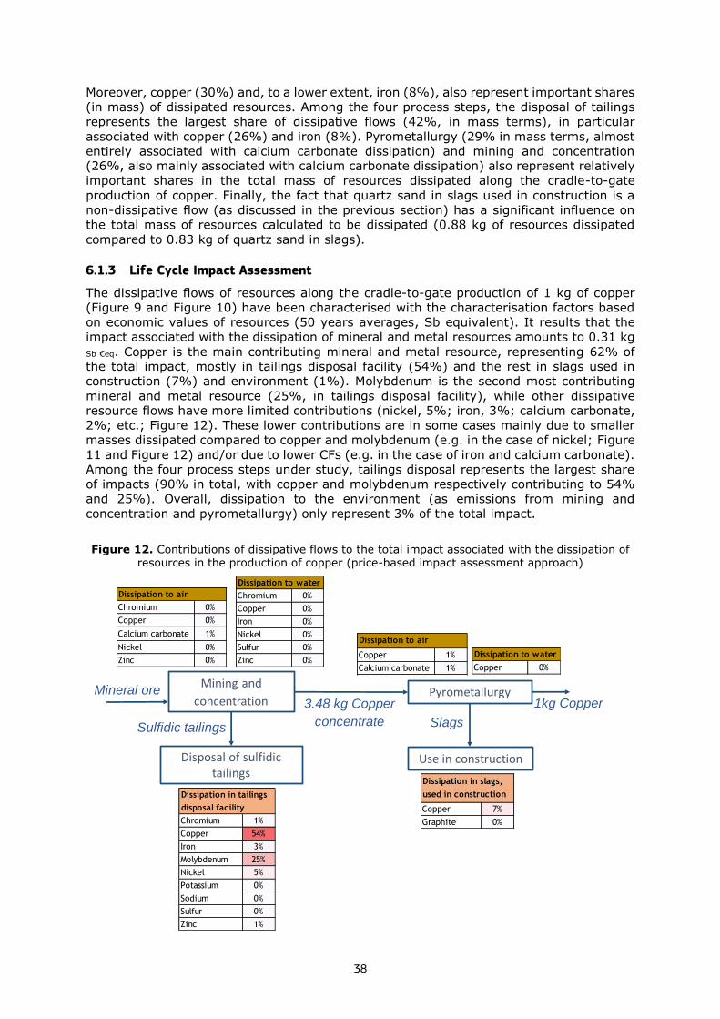
38

Moreover, copper (30%) and, to a lower extent, iron (8%), also represent important shares

(in mass) of dissipated resources. Among the four process steps, the disposal of tailings

represents the largest share of dissipative flows (42%, in mass terms), in particular

associated with copper (26%) and iron (8%). Pyrometallurgy (29% in mass terms, almost

entirely associated with calcium carbonate dissipation) and mining and concentration

(26%, also mainly associated with calcium carbonate dissipation) also represent relatively

important shares in the total mass of resources dissipated along the cradle-to-gate

production of copper. Finally, the fact that quartz sand in slags used in construction is a

non-dissipative flow (as discussed in the previous section) has a significant influence on

the total mass of resources calculated to be dissipated (0.88 kg of resources dissipated

compared to 0.83 kg of quartz sand in slags).

6.1.3 Life Cycle Impact Assessment

The dissipative flows of resources along the cradle-to-gate production of 1 kg of copper

(Figure 9 and Figure 10) have been characterised with the characterisation factors based

on economic values of resources (50 years averages, Sb equivalent). It results that the

impact associated with the dissipation of mineral and metal resources amounts to 0.31 kg

Sb €eq. Copper is the main contributing mineral and metal resource, representing 62% of

the total impact, mostly in tailings disposal facility (54%) and the rest in slags used in

construction (7%) and environment (1%). Molybdenum is the second most contributing

mineral and metal resource (25%, in tailings disposal facility), while other dissipative

resource flows have more limited contributions (nickel, 5%; iron, 3%; calcium carbonate,

2%; etc.; Figure 12). These lower contributions are in some cases mainly due to smaller

masses dissipated compared to copper and molybdenum (e.g. in the case of nickel; Figure

11 and Figure 12) and/or due to lower CFs (e.g. in the case of iron and calcium carbonate).

Among the four process steps under study, tailings disposal represents the largest share

of impacts (90% in total, with copper and molybdenum respectively contributing to 54%

and 25%). Overall, dissipation to the environment (as emissions from mining and

concentration and pyrometallurgy) only represent 3% of the total impact.

Figure 12. Contributions of dissipative flows to the total impact associated with the dissipation of

resources in the production of copper (price-based impact assessment approach)

Mining and

concentrationMineral ore Pyrometallurgy

3.48 kg Copper

concentrateSulfidic tailings


Slags

Use in construction

1kg Copper

Copper 1%


Dissipation to air

Dissipation to air

Chromium 0%

Copper 0%


Nickel 0%

Zinc 0%


Chromium 0%

Copper 0%

Iron 0%

Nickel 0%

Sulfur 0%

Zinc 0%Dissipation to water

Copper 0%

Copper 7%

Graphite 0%

Dissipation in slags,

used in construction

Chromium 1%

Copper 54%

Iron 3%

Molybdenum 25%

Nickel 5%

Potassium 0%

Sodium 0%

Sulfur 0%

Zinc 1%

Dissipation in tailings

disposal facility

39

6.1.4 Comparison with alternatives for inventory and impact assessment

In the following, in order to highlight the influence of some major features of the proposed

approach, a comparison is made with two alternative accounting approaches: respectively,

a long-term perspective for the inventory of dissipative flows, and a (classical) depletion

approach considering resources extracted from the ecosphere instead of resources

dissipated to the ecosphere.

6.1.4.1 Inventory of dissipative flows in a long-term perspective

Firstly, regarding the inventory procedure to trace the dissipative flows at the unit process

level, the first alternative approach considers a very long-term perspective rather than the

short-term perspective. In this long-term perspective, only emissions to the environment

are assumed to render resources “not accessible to future users”; that is to say, only

emissions to the environment are dissipative flows. On the contrary, it is assumed that the

following flows are not dissipative: i) any flow of mineral and metal resource, as such or

embodied in a waste fraction, sent to a final waste disposal facility, and ii) any flow of

mineral and metal resource, as such or embodied in a waste fraction, sent to recovery and

subsequently recovered with low-functionality (including non-functional recycling). The

underlying assumption is that, considering a very long-term perspective, these resources

will be at some point accessible to some future users9.

This alternative scope for the inventory implies focusing on emissions to the environment

only; that is, the dissipative flows representing 3% of the impact when considering the

above-proposed “short-term” approach (see section 6.1.3). Emissions to the environment

associated with tailings disposal (in particular, tailings leachate) are not accounted for in

the short-term perspective, because all resources to tailings disposed of are considered to

be dissipative. Similarly, they are assumed to be negligible as well in the long-term

perspective. It is expected that this assumption has only a limited influence on the impact

assessment result. For example regarding copper, emissions to air from pyrometallurgy

are more than 90 times larger than emissions to water from tailings disposal over 100

years as considered in the ecoinvent database (Doka, 2008a).

This long-term perspective implies a significant shift in main contributions at the level of

both unit processes and resource flows (Table 5): pyrometallurgy is identified as the main

process step (62% of the impact, compared to 2% in the approach tested and presented

in section 6.1.3 in this report), with calcium carbonate as the main contributing resource

(73% of the impact, compared to 2% previously).

6.1.4.2 Inventory and impact assessment using a depletion approach

In the second alternative accounting approach studied, a depletion approach is applied. It

considers the inventory of resources extracted from ground along the cradle-to-gate to

produce 1 kg of copper cathode, combined with the ADP method for impact assessment

(ultimate reserve, with characterization factors as in the EF 3.0 reference package). Both

the extraction of copper and molybdenum from ground in the mining step and the

extraction of resources embodied in products entering the activities (mining and

concentration, and pyrometallurgy) are considered, in order to ensure consistency with the

above-presented case study. As a rough proxy regarding resources embodied in products

entering the activities (e.g. in reagents), it is assumed that the mass of resources extracted

from ground (upstream in the life cycle) is equivalent to that in products. For example,

considering 3.4 g of zinc in reagents entering the unit process of mining and concentration,

per kg of output copper concentrate (Figure 7), it is assumed as a proxy that 3.4 g of zinc

is extracted in the upstream life cycle stages.

9 The very long perspective is an hypothetical and simplified scenario, in which it is assumed that the technological

developments in future will be so advanced to allow the recovery of any resource in very complex waste and matrix (as for example, copper in slags ultimately ending in construction and demolition waste).

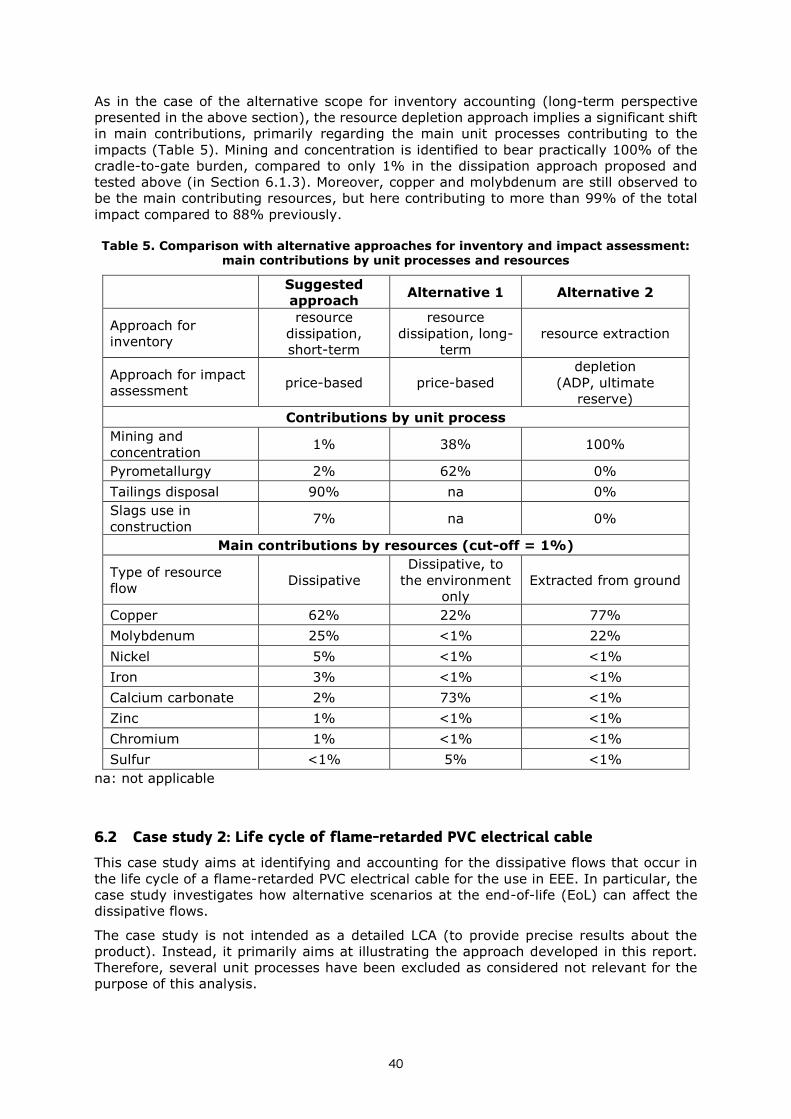
40

As in the case of the alternative scope for inventory accounting (long-term perspective

presented in the above section), the resource depletion approach implies a significant shift

in main contributions, primarily regarding the main unit processes contributing to the

impacts (Table 5). Mining and concentration is identified to bear practically 100% of the

cradle-to-gate burden, compared to only 1% in the dissipation approach proposed and

tested above (in Section 6.1.3). Moreover, copper and molybdenum are still observed to

be the main contributing resources, but here contributing to more than 99% of the total

impact compared to 88% previously.

Table 5. Comparison with alternative approaches for inventory and impact assessment: main contributions by unit processes and resources

Suggested

approach Alternative 1 Alternative 2

Approach for

inventory

resource

dissipation,

short-term

resource

dissipation, long-

term

resource extraction

Approach for impact

assessment price-based price-based

depletion

(ADP, ultimate

reserve)

Contributions by unit process

Mining and

concentration 1% 38% 100%

Pyrometallurgy 2% 62% 0%

Tailings disposal 90% na 0%

Slags use in

construction 7% na 0%

Main contributions by resources (cut-off = 1%)

Type of resource

flow Dissipative

Dissipative, to

the environment

only

Extracted from ground

Copper 62% 22% 77%

Molybdenum 25% <1% 22%

Nickel 5% <1% <1%

Iron 3% <1% <1%

Calcium carbonate 2% 73% <1%

Zinc 1% <1% <1%

Chromium 1% <1% <1%

Sulfur <1% 5% <1%

na: not applicable

6.2 Case study 2: Life cycle of flame-retarded PVC electrical cable

This case study aims at identifying and accounting for the dissipative flows that occur in

the life cycle of a flame-retarded PVC electrical cable for the use in EEE. In particular, the

case study investigates how alternative scenarios at the end-of-life (EoL) can affect the

dissipative flows.

The case study is not intended as a detailed LCA (to provide precise results about the

product). Instead, it primarily aims at illustrating the approach developed in this report.

Therefore, several unit processes have been excluded as considered not relevant for the

purpose of this analysis.

41

Finally, this case-study was built on several different data sources (reports and

publications) in order to get information at the unit process level. Concerning the copper

contained in the cable, results of case-study 1 have been used.

6.2.1 System boundaries

The considered functional unit is 1 kg of electrical cable. The system boundaries of the case

study are illustrated in Figure 13. These include:

- the production of virgin PVC granulates;

- the production of additives: filler (limestone), Antimony Trioxide (ATO) and

plasticizer;

- the production of copper wire (based on results from case study 1);

- three alternatives EoL scenarios for the treatment of the waste cable: Landfill

Scenario; Incineration Scenario; and Recycling Scenario.

Cable production and use phase were excluded because of lack of data and limited

relevance as the main impacts there are associated to energy consumption.

Figure 13 shows: in blue the unit processes included in the analysis; in yellow the unit

processes excluded from the analysis10; and in green the unit processes related to

alternative EoL scenarios.

Figure 13. System boundaries for the analysis of a flame-retarded PVC electrical cable for EEE

10 These units process imply mainly the consumption of energy and have been therefore excluded from the

analysis.

Unit processconsidered

Unit process excluded

Alternative scenarios considered

5. PVC flame retarded

2b. Stibnite mining & refining

2a. Antimony trioxide (ATO)

4. Plasticizer(DOP)

1. PVC(virgin

granulate)

8. Cable use

3. Filler(Limestone)

a) landfill b) incineration c) Recycling

7. Electrical cable production

9. End-of life

6b. Copper wire

6a. Copper production

(case-study 1)

42

6.2.1.1 Polyvinyl Chloride

Polyvinyl chloride (PVC) is manufactured by polymerisation of vinyl chloride monomer

(VCM), which in Europe is produced by the thermal cracking of ethylene dichloride (EDC;

Plastics Europe, 2016). In Europe most ethylene used in the manufacture of EDC is

produced by steam cracking of naphtha. Chlorine is produced by electrolysis of sodium

chloride (NaCl).

There are three commercial processes for the production of PVC: 1) Suspension

polymerisation; 2) Emulsion polymerisation; 3) Bulk or mass polymerisation. Suspension

PVC is the general purpose grade and is used for most rigid PVC applications such as pipes,

profiles, other building materials and hard foils. It is also plasticised and used for most

flexible applications such as cable insulation, soft foils and medical products.

Rigid PVC products (unplasticized) are essentially flame retarded due to their chlorine

content. Plasticized PVC products contain flammable plasticizers and must be flame

retarded. They contain a high enough chlorine content so that an additional halogen is

usually not necessary, and antimony oxide (mainly antimony trioxide – ATO) is used

(USAC, 2017). If plasticizers are used that reduce the halogen content, the halogen content

can be increased by using halogenated phosphate esters or chlorinated waxes. Content of

ATO in PVC flame retarded is generally in the range of 5%-10% (Mihajlović et al., 2010).

6.2.1.2 Additives: flame retardants, fillers, plasticizers

Main application for antimony (Sb) is as ATO used with flame retardant (43% of global end

uses of Sb; EC, 2017). Stibnite (Sb2S3) is the principal ore mineral for the production of

antimony. Antimony trioxide is not a flame retardant in itself but when combined with

halogenated (i.e. brominated or chlorinated) flame retardant compounds it constitutes a

highly-effective flame retardant synergist (EC, 2017). Halogenated antimony compounds

are effective dehydrating agents that inhibit ignition and pyrolysis in solids, liquids and

gases. They also promote the formation of a char-rich layer on the substrate, which reduces

oxygen availability and volatile-gas formation (Schwarz-Schampera, 2014). ATO is

considered one of the best additives for flame retarded PVC (Zhang et al., 2014).

Fillers are added to the PVC resin mix to lower material costs, to provide colouring, Ultra

Violet protection and lubrication. Limestone (calcium carbonate) is the most prevalent filler

used for PVC (Gilbert and Patrick, 2017).

Plasticizers are additives that increase the plasticity or decrease the viscosity of the

plastics. Dioctyl Phthalate (DOP) is one of the most common plasticizer used for PVC

(Zhang et al., 2014).

6.2.1.3 Copper content

It is assumed that the electrical cable has a 33% copper content and 67% plastics (van

Tichelen et al., 2015). Resources dissipated for the production of copper have been referred

to case study 1 (Section 6.1).

6.2.1.4 End of life treatment of PVC cables

Three main EoL routes are supposed for the cable:

- in the Landfill Scenario (9a), the cable is supposed to be directly landfilled (with the

electronic product to which it belongs). Although this practice is not compliant with

the legislation (i.e. EU Directive 2012/19/EU), this is still largely occurring in the EU

especially concerning small household appliance (EUROSTAT, 2019). Once in the

landfill, and considering the 25-year temporal perspective as set in the proposed

approach to account for resource dissipation (section 4.2), there is little chance that

either the plastics or metals in the cables could be recovered.

43

- in the Incineration Scenario (9b) the cable is supposed to be directly incinerated

(together with the electronic product to which it belongs). This practice allows the

energy recovery, while only a fraction of some metals (e.g. aluminium, copper, zinc

and ferrous metals) could be potentially recovered from bottom ashes. However,

these recovery processes imply complex processing (including high environmental

impacts) and are characterised by variable efficiency and yields (Lassesson et al.,

2014; Bunge, 2015), so that, generally, the majority of materials is not recovered

(e.g. the antimony used in the plastics additives; EC, 2017). Therefore, in this case

study, recovery of materials from bottom ashes is not considered.

- in the Recycling Scenario (9c), the cable is supposed to be disassembled/dismantled

from the product and afterwards shredded, allowing the separation of copper (for

recycling) from plastics (sent to incineration as in scenario 9b).

6.2.2 Life Cycle Inventory

Information about the processes and life cycle inventory data used for the case study are

derived from the literature. However, a single data source, sufficiently disaggregated to

estimate dissipative flows for all the considered unit processes, was not available.

Therefore, different references (journal articles and reports) have been used, as illustrated

in Table 6. Since the demonstrative purpose of the case-study, an assessment of the

quality of used data has not been performed.

Similarly to the approach undertaken in the case study 1, fossil fuels and energy sources

have not been traced (out of scope for this analysis), while resources for capital equipment

and blasting have been disregarded.

Table 6. Detail of main assumptions and data sources for the life cycle inventory

Data References

Composition of plastic in electrical

cable:

PVC 100 – Filler 50 - Plasticizer (DOP)

40 – Flame retardant (ATO) 10

PVC4Cables, 2017

Composition of cable: plastics (67%);

copper (33%). van Tichelen et al., 2015

Production of PVC (including also the

production of Chlorine from NaCl

electrolysis)

Simonson et al. 2000; Boustead,

2005; Plastics Europe, 2016

Production of ATO (including stibnite

mining, crushing, grinding, flotation,

drying, and oxidation)

Simonson et al., 2000; Jonkers et al.,

2016

Production of limestone

Ecoinvent 2: limestone quarry

operation; limestone production,

crushed, for mill; lime production,

milled, loose; all these inventories

relative to Switzerland (CH;

ecoinvent, 2019)

Production of DOP Not considered, due to the absence of

any available reference

Incineration of electrical cable Doka, 2008b

The next phase of the analysis concerns the calculation of the dissipative flows of resources

for each step considered (Figure 13). The calculation implied to identify the resource in

44

input and output of the unit process, and to trace dissipative flows that occur in the output

compartments (e.g. emissions to air, emissions to water and emissions to waste11).

Figure 14 shows the detail of the accounting for the unit process relative to the virgin PVC

production (“Step 1”). Concerning the resource in input, chlorine (the “target element”)

has been considered in place of NaCl (see Section 4.1). However, other options could

consider differently resource as inputs (e.g. NaCl in place of Cl; see Section 4.1) and it

could be the object of future explorations.

Moreover, the inventory is also including emissions to air and water as due to the

foreground process of electrolysis of NaCl to produce chlorine. These emissions have been

then analysed to identify potential dissipative flows (e.g. emissions of sodium and

mercury12).

When necessary, the flow data have been adjusted in order to match the mass balances.

For example, input chlorine has been determined as the stoichiometric amount of chlorine

in PVC plus the chlorine in air and water emissions. In the case of emissions of hydrochloric

acid (HCl), only chlorine has been considered as the resource dissipated. As discussed in

section 7.1.2.2, emissions of nitrogen or sulphur have been excluded since they do not

refer to resources in inputs (due to e.g. combustion).

Figure 14. Dissipative flows of resources in the production of virgin PVC (step 1 of the case study).

11 Due to the lack of detailed information on the waste, it was not possible to differentiate among flows to different

sub-compartment (e.g. tailings, slag, ashes, landfill). These flows have been therefore grouped in a single category.

12 Mercury cell method was used to produce chlorine in the chlor-alkali process. Since this process has been

nowadays phased-out, emissions of mercury have been excluded.

STEP 1. PVC (virgin) production

PVC production(virgin granulate)

Water

Emissions to air:

CO2 : 1.944 kgCO : 0.0027 kgHC (unspecified): 0.02 kgHC (chlorinated): 0.00072 kgHCl: 0.00023 kgHg: 2.70E-07 kgNOx: 0.016 kgParticulate (unspecified): 0.0039 kgSO2 : 0.013 kg

Emissions to water:Acids: 0.00011 kgBOD: 8.00E-05 kgChloride ions: 0.04 kgCOD: 0.0011 kgHC (chlorinated): 1.00E-05 kgHg: 5.60E-08 kgOil: 5.00E-05 kgSodium ions: 0.0023 kgSulphate ions: 0.0043 kgTSS: 0.0024 kg

PVC 1 kg

0.5677 kg Cl

Cl: 0.000224 kg

Other Inputs:

Limestone (CaCO3): 0.0016 kgSand : 0.0012 kg

Other resources (assumed as capital eq.):

Bauxite: 0.00022 kgIron (ore): 0.0004 kg Assumed ending

in waste

Limestone (CaCO3): 0.0016 kgSand : 0.0012 kg

Energy carriers:

Chlorine: 0.61 kg

0.61 kg Cl

Waste: Hazardous waste: 0.0012 kgIndustrial waste: 0.016 kgMineral waste: 0.066 kgSlag and Ash: 0.047 kg

Colour Legend:

Resource flows consideredDissipative resource flowsExcluded flowsOther flows (undefined)

45

Table 7 summarizes the dissipative flows of resources occurring in the studied steps. Note

that the three scenarios differ only for the last step (on EoL). Scenario 9b differ from 9c

only about copper, which is considered recycled in 9c whereas dissipated in scenario 9b.

Table 7. Detail of dissipative flows for the production of 1 kg of Electrical Cable in the three compartments, for the three different EoL scenarios

6.2.3 Life Cycle Impact Assessment

The dissipative flows per kg of electrical cable (Table 8) have been characterised with the

characterisation factors based on economic values of resources (50 years averages; Sb

reference resource; see section 5.3.1). It results that in the Landfill Scenario, the

dissipated resources amount to 0.584 kg Sb €eq (all the resources are assumed to be

dissipated due to landfilling). This value slightly raises in the Incineration Scenario (due to

the consumption of the reagents for the incineration process13). The amount of dissipative

13 Benefits related to energy recovery are not accounted for.

1- PVC 2-Sb 3-filler 6- Cu 9a)EoL 1- PVC 2-Sb 3-filler 6- Cu 9b)EoL 1- PVC 2-Sb 3-filler 6- Cu 9c) EoL

Cl 2.2E-04 2.2E-04 2.1E-06 2.2E-04 2.1E-06

Ca 1.1E-04 1.1E-04

CaCO3 1.8E-04 4.5E-01 1.8E-04 4.5E-01 1.8E-04 4.5E-01

Cr 5.7E-06 5.7E-06 5.7E-06

Cu 2.8E-03 2.8E-03 2.8E-03

Ni 4.5E-06 4.5E-06 4.5E-06

Sb 4.5E-08 4.5E-08 1.1E-10 4.5E-08 1.1E-10

Zn 1.1E-05 1.1E-05 1.1E-05

Cl 4.0E-02 4.0E-02 1.9E-01 4.0E-02 1.9E-01

Cr 9.6E-08 9.6E-08 9.6E-08

Fe 5.1E-05 5.1E-05 5.1E-05

Na 2.3E-03 2.3E-03 2.3E-03

Ni 4.3E-06 4.3E-06 4.3E-06

S 2.8E-02 2.8E-02 2.8E-02

Sb 9.7E-03 9.7E-03

Ca 2.5E-04 2.5E-04

Cu 1.6E-06 1.6E-06 1.1E-05 1.6E-06 1.1E-05

Zn 1.3E-05 1.3E-05 1.3E-05

Ca 2.3E-02 2.3E-02

Cr 1.7E-02 1.7E-02 1.7E-02

Cl 1.9E-01 6.3E-03 6.3E-03

Cu 2.6E-01 3.3E-01 2.6E-01 3.3E-01 2.6E-01

Fe 6.8E-02 6.8E-02 8.0E-04 6.8E-02 8.0E-04

Graphite 1.0E-03 1.0E-03 1.0E-03

K 5.7E-03 5.7E-03 5.7E-03

S 1.4E-02 1.4E-02 1.4E-02

Sb 2.8E-02 1.8E-02 1.8E-02

CaCO3 1.6E-03 1.8E-04 1.7E-01 1.6E-03 1.8E-04 1.7E-01 1.6E-03 1.8E-04 1.7E-01

Mo 1.9E-02 1.9E-02 1.9E-02

Na 2.0E-03 2.0E-03 1.1E-01 2.0E-03 1.1E-01

Ni 7.3E-03 7.3E-03 7.3E-03

Sand 1.2E-03 8.3E-01 1.2E-03 8.3E-01 1.2E-03 8.3E-01

Zn 1.2E-02 1.2E-02 1.2E-02

Dissipated

resources 4.5E-02 4.5E-08 3.5E-04 1.7E+00 7.2E-01 4.5E-02 4.5E-08 3.5E-04 1.7E+00 8.5E-01 4.5E-02 4.5E-08 3.5E-04 1.7E+00 5.2E-01

Total [kg] 2.48 2.61 2.28

Dissipation to water [kg]

Dissipation to waste disposal [kg]

Dissipation to air [kg]

SCENARIO (landfill) - STEPS SCENARIO (incineration) - STEPS SCENARIO (Recycling) - STEPS

46

resource flows is significantly lower in the Recycling Scenario (-65%), thanks to the

assumption that copper scraps are separated for being recycled (and therefore are not

dissipated). The scenarios did not consider, anyway, the potential dissipative flows

occurring during the recycling process of copper scraps to produce secondary copper.

Table 8. Impact assessment of dissipative flows for 1 kg of electrical cable (as kgSb €eq.)

Table 9 finally shows the percentage contribution of each step and compartment. Overall,

emissions to air and water generally have negligible or very low contributions (below 2%),

1 2 3 6 9a 1 2 3 6 9b 1 2 3 6 9c

Cl 1.3E-06 1.3E-06 1.2E-08 1.3E-06 1.2E-08

Ca 1.7E-06 1.7E-06

CaCO3 2.7E-06 6.7E-03 2.7E-06 6.7E-03 2.7E-06 6.7E-03

Cr 1.3E-06 1.3E-06 1.3E-06

Cu 2.0E-03 2.0E-03 2.0E-03

Ni 9.9E-06 9.9E-06 9.9E-06

Sb 4.5E-08 4.5E-08 1.1E-10 4.5E-08 1.1E-10

Zn 3.4E-06 3.4E-06 3.4E-06

Cl 2.3E-04 2.3E-04 1.1E-03 2.3E-04 1.1E-03

Cr 2.2E-08 2.2E-08 2.2E-08

Fe 6.1E-06 6.1E-06 6.1E-06

Na 1.3E-05 1.3E-05 1.3E-05

Ni 9.3E-06 9.3E-06 9.3E-06

S 5.0E-04 5.0E-04 5.0E-04

Sb 9.7E-03 9.7E-03

Ca 3.8E-06 3.8E-06

Cu 1.2E-06 1.2E-06 8.3E-06 1.2E-06 8.3E-06

Zn 4.1E-06 4.1E-06 4.1E-06

Ca 3.5E-04 3.5E-04

Cr 3.8E-03 3.8E-03 3.8E-03

Cl 1.1E-03 3.6E-05 3.6E-05

Cu 1.9E-01 2.4E-01 1.9E-01 2.4E-01 1.9E-01

Fe 8.1E-03 8.1E-03 9.6E-05 8.1E-03 9.6E-05

Graphite 9.9E-05 9.9E-05 9.9E-05

K 2.6E-04 2.6E-04 2.6E-04

S 2.5E-04 2.5E-04 2.5E-04

Sb 2.8E-02 1.8E-02 1.8E-02

CaCO3 2.4E-05 2.7E-06 2.5E-03 2.4E-05 2.7E-06 2.5E-03 2.4E-05 2.7E-06 2.5E-03

Mo 7.8E-02 7.8E-02 7.8E-02

Na 1.2E-05 1.2E-05 6.1E-04 1.2E-05 6.1E-04

Ni 1.6E-02 1.6E-02 1.6E-02

Sand 4.9E-06 3.4E-03 4.9E-06 3.4E-03 4.9E-06 3.4E-03

Zn 3.6E-03 3.6E-03 3.6E-03

Dissipated

resources2.7E-04 4.5E-08 5.3E-06 3.1E-01 2.7E-01 2.7E-04 4.5E-08 5.3E-06 3.1E-01 2.7E-01 2.7E-04 4.5E-08 5.3E-06 3.1E-01 3.3E-02

Total [kg Sb €eq] 0.3440.583 0.584

Dissipation to water [kg Sb €eq]

Dissipation to waste disposal [kg Sb €eq]

Dissipation to air [kg Sb €eq]

SCENARIO (incineration) - STEPS SCENARIO (Recycling) - STEPSSCENARIO (landfill) - STEPS

47

while the impacts are mainly related to the resources ending in waste. In the landfill and

incineration scenarios, the copper production (step 6) is the step causing the largest

impact, due to dissipative flows of copper and molybdenum (mainly in tailings, as discussed

in case study 1). Afterwards, the EoL treatments (steps 9a and 9b) are the steps with the

highest impact, mainly due to the dissipative flows of copper in the electrical cable.

As mentioned, in the Recycling Scenario the copper in the cable is supposed to be extracted

to being recycled, and therefore the impact of the step 9c largely decreases. In this

scenario, the contribution of the impact of other dissipative flows slightly rises, as for

instance the antimony contained in the cable’s plastics and that is dissipated in incineration

ashes (about 5% of the overall impact).

Table 9. Impact assessment: contributions of the different dissipative flows

1- PVC 2-Sb 3-filler 6- Cu 9a)EoL 1- PVC 2-Sb 3-filler 6- Cu 9b)EoL 1- PVC 2-Sb 3-filler 6- Cu 9c)EoL

Cl negl. negl. negl. negl. negl.

Ca negl. negl.

CaCO3 negl. 1.1% negl. 1.1% negl. 1.9%

Cr negl. negl. negl.

Cu 0.3% 0.3% 0.6%

Ni negl. negl. negl.

Sb negl. negl. negl. negl.

Zn negl. negl. negl.

Cl negl. negl. 0.2% negl. 0.3%

Cr negl. negl. negl.

Fe negl. negl. negl.

Na negl. negl. negl.

Ni negl. negl. negl.

S 0.1% 0.1% 0.1%

Sb 1.7% 2.8%

Ca negl. negl.

Cu negl. negl. negl. negl. negl.

Zn negl. negl. negl.

Ca 0.1% 0.1%

Cr 0.7% 0.7% 1.1%

Cl 0.2% negl. negl.

Cu 32.3% 41.2% 32.3% 41.1% 54.9%

Fe 1.4% 1.4% negl. 2.4% negl.

Graphite negl. negl. negl.

K negl. negl. 0.1%

S negl. negl. 0.1%

Sb 4.8% 3.1% 5.3%

CaCO3 negl. 0.4% negl. 0.4% negl. 0.7%

Mo 13.4% 13.4% 22.7%

Na negl. negl. 0.1% negl. 0.2%

Ni 2.7% 2.7% 4.7%

Sand negl. 0.6% negl. 0.6% negl. 1.0%

Zn 0.6% 0.6% 1.0%

Contr.to

impact [%]negl. negl. negl. 53.4% 46.6% negl. negl. negl. 53.3% 46.7% negl. negl. negl. 90.4% 9.5%

negl.: negligible (<0.1%)

Dissipation to water [kg]

Dissipation to waste disposal [kg]

SCENARIO (incineration) - STEPS SCENARIO (Recycling) - STEPS

Dissipation to air [kg]

SCENARIO (landfill) - STEPS

48

7 Suggested approach for the impact assessment of biotic

resources

7.1 State of the art of naturally occurring biotic resources in LCA

Currently, naturally occurring biotic resources are not properly addressed in LCA. On one

hand, life cycle inventories lack a complete list of elementary flows for natural biotic

resources. On the other hand, models for a comprehensive characterization of impacts due

to the exploitation of naturally occurring biotic resource are very few (Crenna et al. 2018).

The identification of the elementary flows needs a considerable effort in order to establish

a harmonized and unified reference terminology within the inventories. Moreover, for

naturally occurring biotic resources (NOBR) some specific aspects, like the ecological

properties together with the geographical localization of the extraction of the resources,

are fundamental in view of a complete analysis. The characterization of the impacts from

the extraction of natural biotic resources is complex and to date, an agreed model for the

characterization of biotic resources exploitation is missing. Although impacts on

ecosystems due to different impact categories are considered within the Area of Protection

“Ecosystem Quality”, damages to biotic resources related to their depletion (such as

overharvesting, overfishing, and overhunting) remain not accounted.

So far, only few attempts have been made to include impacts of biotic resources extraction

using different models and indicators.

Other models are thermodynamically-based. For example, exergy- based LCA models such

as Dewulf et al. (2007), Alvarenga et al. (2013), Taelman et al. (2014), aim at assessing

the quality of resources depending on the amount of useful energy needed for producing

them and that could be obtained from them. Besides, emergy-based LCA model (Rugani

et al., 2011) aims at measuring the Solar Energy Demand (SED) associated with the

extraction of resources, including both naturally occurring and man-made biotic ones.

Langlois et al. (2014) proposed quantitative approaches to address overfishing at the

midpoint level, the authors developed a methodological framework to assess impacts of

fish depletion at both species and ecosystem levels. Langlois et al. (2014) model is based

on the concept of biotic resource depletion for fish, which aims to characterize the current

biomass uptake related to either the Maximum Sustainable Yield (MSY, based on fisheries

science) or the current fish catches (Ct) in case of overexploitation. This model, which

provides characterization factors for 127 fish species, allows evaluating the potential

impacts associated to fisheries wild catch, in a context where one third of global fish stocks

is already overexploited. The study is the first attempt to assess impacts on the use of

biotic resources taking into account ecological aspects such as the resource recovery

capacity.

In parallel with the study of Langlois et al. (2014), Emanuelsson et al. (2014) focused on

the concept of Lost Potential Yield (LPY) for fish, proposing new characterization factors for

31 European fish species. The model aims at measuring and characterizing the current

overexploitation of natural fish stocks, suggesting a midpoint indicator that allows

identifying the impacts on the reduction of future fish supply.

Bach et al. (2017) proposed the BIRD approach, inspired by the abiotic depletion potential

(van Oers et al., 2002). The BIRD model focuses on terrestrial biotic resources and it

measures the availability of biotic resources by using the Biotic Resource Availability (BRA)

indicator (defined as availability to use ratio). In their proposal, the authors include

considerations on the replenishment rate and the identification of a reference species.

Differently from other models, in this approach, several aspects beyond the ecological

constraints are taken into account (e.g. socio-economic aspects).

Hélias et al. (2018) developed characterization factors for fish, globally. These

characterization factors convert the mass of captured fish into a variation of depleted stock

fraction (DSF), taking into consideration information on fish catches, stock biomass and

the maximum intrinsic rate of population increase.

49

7.2 Characterisation models for the impact assessment of natural biotic

resources

In this study, a comprehensive four-step approach to characterize the impacts due to the

overexploitation of naturally occurring biotic resources in LCA has been developed. In the

first step, available data on natural occurring biotic resources (NOBR) having a commercial

value were collected. These data were used to build a list of elementary flows to be used

in future life cycle inventories. NOBR are commercially valuable resources proceeding from

biological sources that are caught or harvested from the ecosphere as input material for

human purposes (e.g. wild foods, wild wood, etc.) (Crenna et al., 2018). In the second

step, an indicator based on the ecological characteristics of the species was developed.

This indicator called “renewability indicator” aims at distinguishing species based on the

amount of years necessary to produce one kg of the biotic resource. Finally, in the third

step, two scores reflecting the overall availability of the NOBR were developed. One

associated with the current level of exploitation of the species in the wild, called

exploitation score, and another one reflecting the level of extinction threat a species is

subjected to. In the fourth step, characterization factors are calculated combining the

renewability indicator and the exploitation and vulnerability scores. Soils are not considered

in this study. Although they are potentially subject to regenerate over time, they should

not be considered a NOBR, since soils are considered non-renewable resources (soil

formation processes take very long to occur, and therefore soils are not recoverable within

a human lifespan) (EC, 2006).

7.2.1 Elementary flows of natural occurring biotic resources (NOBR)

In order to build a list of the resources commercially valuable proceeding from biological

sources (i.e. plants, animals and other organisms) that are caught or harvested from

ecosphere as input material for human purposes, we consulted specific reports and

databases, such as, just to name a few, Food and Agriculture Organization of the United

Nations (FAO) databases for forestry and fishery statistics (FAO 2016a, b), Artemis-face

database from the European Federation of Hunters for game hunting information (FACE,

2016) and the International Union for Conservation of Nature (IUCN) red list of threatened

species (IUCN, 2016). Thus, by collecting and combining data from different sources, we

identified and integrated a list of NOBR, excluding those proceeding from agriculture,

aquaculture and livestock, since they depend on human interventions (Annex 4). This list

could be the basis for a list of elementary flows to be used in life cycle inventories.

Moreover, we sought for data on biotic resource availability, use, and consumption to

understand how these resources are distributed and shared within the markets at different

scales, both local and global. The data on availability and consumption have been collected

to demonstrate that the resource is used somewhere in the economy, so is a resource used

by humans. This step is fundamental to identify the biotic resources currently used and,

hence, for which of them data may be available, in future, for populating life cycle

inventories.

We have classified NOBRs in the following major categories, according to their taxonomic

level (Table 10): aquatic and terrestrial vertebrates, aquatic and terrestrial invertebrates,

terrestrial plants, aquatic plants and algae, fungi, aquatic and terrestrial animal products,

terrestrial plant products. According to our analysis, naturally occurring biotic resources

are most commonly used as material input in a broad array of industrial sectors, ranging

from food to chemical and pharmaceutical sectors, up to production of e.g. furniture.

Together with their derived products, they are generally used as commercial goods

marketed at global level, in terms of food and feeding, as source of energy, in the

cosmetics, as medicines and for the production of other accessories in different branches

of the industrial sector (e.g. natural pearls, natural latex). Several natural biotic resources,

such as wild plants, are used in local communities, especially in the developing countries,

as dyes, poisons, shelter, fibres and in religious and cultural ceremonies (Heywood, 1999).

50

In spite of the recognized role of naturally occurring biotic resources in human daily life,

accurate data on their availability and renewability rate were difficult to gather among

scientific literature. On one hand, this may be because most countries, especially the

developing ones, have less or no official supervision on the volume of biotic material

harvested from the wild and quantities collected are scarcely inventoried. On the other

hand, it is often difficult to distinguish between wild and cultivated resources, especially in

the case of wild plants, as such primarily wild-collected products are often sold as cultivated

(Kuipers, 1997). Some information exists on a reduced number of natural biotic products;

however, the available data are extremely variable in coverage and reliability. In fact, the

majority of retrieved data were scattered among reports and databases proceeding from

different sources, disciplines and institutions, reporting information limited to some specific

locations.

It is worth noting that, even though naturally occurring biotic resources are spread around

the world and the overwhelming majority of them are commercially used on a global scale,

so far a complete list was missing within the available literature. An important attempt was

made by Schulp et al. (2014), who reported and mapped the ecosystem service called

“wild food”, quantifying the supply of terrestrial edible species (i.e. game, mushrooms and

vascular plants) across Europe. Gathering a broad list of around 130 species based

primarily on their commercial use allows us to start connecting natural biotic resources to

elementary flows within the LCA framework (see Annex 4 and Crenna et al. 2018).

Table 10. Number of NOBRs identified per taxonomic category (for full list see Annex 4.).

Category Number of

NOBRs

identified

Aquatic vertebrates 63

Terrestrial Vertebrates 19

Terrestrial invertebrates 7

Terrestrial plants 32

Aquatic plants and algae 3

Fungi 1

Aquatic animal products 9

TOTAL 134

7.2.2 Renewability indicator

The renewability indicator is the starting point for the characterization of NOBR (Figure

15). This indicator builds upon ecological traits of different species, which may determine

a threat to conservation and resource provision. Generally, a NOBR with longer renewability

time would imply higher risk of depletion if the carrying capacity is overcome.

Based on an extensive literature review, a number of different renewability indicators

(population doubling time, populations size/stock recovery time, population cycle, biomass

recovery time, regeneration time and rotation period) were identified. It was difficult to

find homogenous indicators for all NOBRs except for fish, few other animals and plants.

Therefore, by capitalizing on the available indicators and data, two indicators, population

doubling time for wildlife and rotation period for plants were selected. So far these two

indicators represent the best quantitative proxy of the key features affecting the resource

availability potential. If a single value was not available, we calculated the renewability

indicator (see Annex 5 and Crenna et al. 2018) as arithmetic mean between the maximum

and the minimum values of the renewal time ranges proposed in the retrieved literature.

In several cases (e.g. Brown trout, Atlantic sturgeon), due to the lack of a properly defined

range of time, we used the maximum or minimum presented value as absolute average

51

value for the calculation of the renewability indicator. The unit of measurement is years/kg

so that this indicator can be multiplied by elementary flows expressed in terms of mass.

Figure 15. Cause – effect chain of the impacts associated to the use of naturally occurring biotic

resources and the characterization of their availability. PDF stands for potentially disappeared fraction of species. The full line indicates the characterisation model developed in this report.

Adapted from Crenna et al. (2018).

The renewability indicator is the starting point for the characterization of NOBR. However,

renewability alone does not provide any information about the current level of pressures a

certain species is facing, which is fundamental to assess potential risk of overexploitation.

More specifically, it does not inform about the extent to which the resource is available nor

about its current state. To address these elements, in the next sections, a qualitative

approach to reflect resource availability is proposed, based on current level of exploitation

(sustainability) and vulnerability scores.

7.2.3 Exploitation scores

The purpose of including an exploitation score is to be able to reflect the current

exploitation state of the NOBR. This is important, because it will directly affect the

renewability potential of a resource. In general terms a resource can be overexploited (if

it is harvested at a higher rate than it can be renewed), exploited (if it is harvest at the

same rate it can be renewed) or underexploited (if it is extracted at a lower rate that it can

be renewed).

The exploitation scores were defined for: 1) fish; 2) forest, 3) other wild species. The

exploitation scores can be defined by considering the level of exploitation of a certain

NOBR. Next, we present the theoretical background for the definition of the exploitation

score.

7.2.3.1 Fish

An important concept to determine the level of exploitation of fish stocks is the Maximum

Sustainable Yield (MSY). MSY is the largest catch that can be taken from a certain fish

stock, sustainably, over an indefinite period. The MSY refers to a point of equilibrium

between the exploited population and the fishing activity. A fish stock is said to be

overexploited if its catch surpasses the MSY, exploited if the catch is close to MSY, or

underexploited if the catch is lower than MSY (Helias et al. 2018).

Two useful indicators to understand the level of exploitation of a fish stock are:

F/FMSY: For quantification purposes stock mortality due to fishing, F, is expected to be

close to the F that produces maximum sustainable yield (FMSY). As such the ratio F/FMSY

is used to indicate fishing pressures on fish stocks. Values above 1.0 show that the current

fishing mortality exceeds FMSY, indicating that the stock is not exploited at its maximum

long term potential.

52

B/BMSY: Similarly, since the main goal is to have fish stocks at a biomass level that allows

for the maximum stock growth (BMSY), it is compared the current stock biomass (B) to

the BMSY. Values below 1.0 show that the current stock biomass is below BMSY, indicating

that the stock is not at its optimal size.

There are several sources of information regarding the level of exploitation of fish stocks

(for example, FAO (2011), Ricard et al. (2012), FAO (2018) and STECF (2018).

7.2.3.2 Forest

The rationale used to keep a forest resource intact at the landscape level is to remove less

timber than it is grown annually (O’Brien and Bringezu, 2017). The commonly used

indicator to assess the sustainable use of forest resources is an indicator associated with

timber removal – the net annual increment (NAI). To sustainably harvest timber resources

harvesting should be kept below the NAI. Net annual increment is the average annual

volume over the given reference period of gross increment minus the volume of natural

losses on all trees with a certain diameter (EEA, 2017). The harvest or annual fellings is

the average annual standing volume of all trees (living or dead) that are felled during a

period, including the volume of trees or parts of trees that are not removed from the forest,

other wooded land or other felling site (EEA, 2017).

To allow regeneration, a certain amount of biomass should not be removed. The threshold

established by the European Environmental Agency (EEA) is 70%. If more than 70% of the

NAI is harvested, then the forest is considered to be overexploited. It is important to keep

in mind that this threshold is location-specific, and that it is depended on the forest

structure (type and age of the forest), management practices and also on the goals

established for that forest (for example, if the goals are to maintain biodiversity and the

ecosystem services provided by the forest, it is unlikely that the 70% threshold would be

enough) (Schulze et al., 2012, O’Brien and Bringezu, 2017).

It has to be noted that there is a lack of data availability to perform such an assessment

at the global level. Moreover, this information is not available at the species level; the level

of the renewability indicators from Crenna et al. (2018). A pragmatic solution at this stage

would be to adopt a global default value based on the EU threshold – the resource will be

considered overexploited if more than 70% of the NAI is harvested.

7.2.3.3 Other wild species

The assessment of the level of exploitation of other wild species followed the same principle

as explained before: harvest levels should be kept below the regeneration levels.

Overexploitation is one of the main drivers of biodiversity loss (Pereira et al. 2012).

However, to establish the extent to which a certain population of a NOBR is overexploited

requires data that are not regularly collected or kept at a global level. Such analysis would

need to be therefore case specific.

For example, Harris et al. (2015) identified overexploited bird species due to wild bird

trade, based on expert-opinion information and market data. They characterized 38 species

of Indonesian birds and found that 14 species undergone population declines that could be

attribute to the pet trade.

7.2.4 Vulnerability scores

To establish the vulnerability score we use the International Union for Conservation of

Nature (IUCN) Red List of Threatened species (hereafter Red List) (IUCN, 2019). The Red

List informs about species risk of extinction by categorizing them in 9 possible categories

(Table 11). For each category a vulnerability score can be assigned, ranging for example

53

from 1 (no known extinction risk) to 5 (a species that is critically endangered in the wild).

The categories “Extinct in the wild” and “Extinct” are not taken into consideration since, by

definition, these species are not available anymore in the wild and therefore would not

classify as NOBR.

Table 11. Definition of the Red List categories (IUCN, 2019; Rodrigues et al., 2006).

Threat category

Acronym Definition

Extinct EX A species to which there is no reasonable doubt that the last individual has died.

Extinct in the wild

EW A species know to survive only in cultivation, captivity or as a naturalized population, well outside the past range.

Critically endangered

CR A species facing a high risk of extinction in the wild.

Endangered EN A species facing a high risk of extinction in the wild.

Vulnerable VU A species facing a high risk of extinction in the wild.

Near threatened

NT A species that is close to classifying to a higher extinction risk.

Least concern LC A species that does not qualify for higher extinction risk.

Data deficient DD Not enough available information to assess the risk of extinction of a species, based on its distribution and or

population status.

Not evaluated NE Species not evaluated against Red List criteria.

7.2.5 Characterization of NOBR taking into account renewability and level of exploitation

We propose an approach to characterize biotic resources that complements the

renewability indicator with information that reflects the level of exploitation of the resource

(Figure 15). The exploitation score informs on the status of the resource populations being

exploited, and vulnerability scores, that inform on species risk of extinction. Considering

these two elements in the characterization factor (CF) is important because renewability

alone does not inform on the status of the resource being exploited, nor on other pressures

impacting the NOBR.

Our modelling approach uses the exploitation (ES) and vulnerability (VS) scores as

penalization factors for the renewability indicator. If a NOBR is underexploited and it is not

threatened then the characterization factor (CF) will always be equal to the renewability

indicator (RI).

Since the scores translate a qualitative information into a numerical value, the choice of

the scores might have a great influence on the final CFs. Therefore, in the next section,

four options to attribute scores are reported. In all options, we opted to give a score of 1

to Data Deficient (DD) and Not Evaluated (NE) species because there is not enough

information to establish the threat category of these species. According to IUCN, a species

is DD when there is inadequate information to make a direct, or indirect, assessment of its

risk of extinction based on its distribution and/or population status (IUCN, 2001). DD

assignment does not mean that the species is not well studied, instead it means that

appropriate data on abundance and/or distribution is missing. IUCN (2001) recommends

care in the attribution of this category and that the precautionary principle should be

followed. For example, if the range of a species is suspected to be small and a considerable

period of time has passed since the last record of the taxon then a threatened status is

justified instead of a DD status (IUCN, 2001).

54

7.2.5.1 Option 1

In this option, we consider the following discrete values for the vulnerability scores and

exploitation scores:

Table 12. Vulnerability and exploitation scores used in option 1.

Threat category Vulnerability

score (VS)

Exploitation

status

Exploitation

score (ES)

Critically endangered (CR) 5 Depleted 4

Endangered (EN) 4 Overexploited 3

Vulnerable (VU) 3 Exploited 2

Near threatened (NT) 2 Underexploited 1

Least concern (LC) 1

Data deficient (DD) 1

Not evaluated (NE) 1

And we computed the characterization factor, for each NOBR i, as follows:

CFi = Renewability indicator (RIi) x Exploitation score (ESi) x Vulnerability score (VSi)

In order to test this option, we created 100 hypothetical NOBRs to which we randomly

attributed a renewability indicator (between 1 and 50 years/kg, which matches the

identified range, for animals, of the renewability indicator presented in Section 7.2.2), an

exploitation score (between 1 and 4) and a vulnerability score (between 1 and 5).

The values obtained for the CF range between 13.1 years/kg (Min) and 925.5 years/kg

(Max). Most of the CF values are below 500 (Figure 16). It is possible to find NOBRs with

high VS (yellow) and high ES (bigger circles) and low RI with a low CF, as well as very

threatened species (high VS) with low CF. Ideally, the range of CFs for species very

threatened and very exploited would be reduced.

Figure 16. Characterization factor (in years/kg) for option 1. The size of the circles

represent the value of the exploitation score (ES), the colours of the circles represent the

vulnerability score (VS).

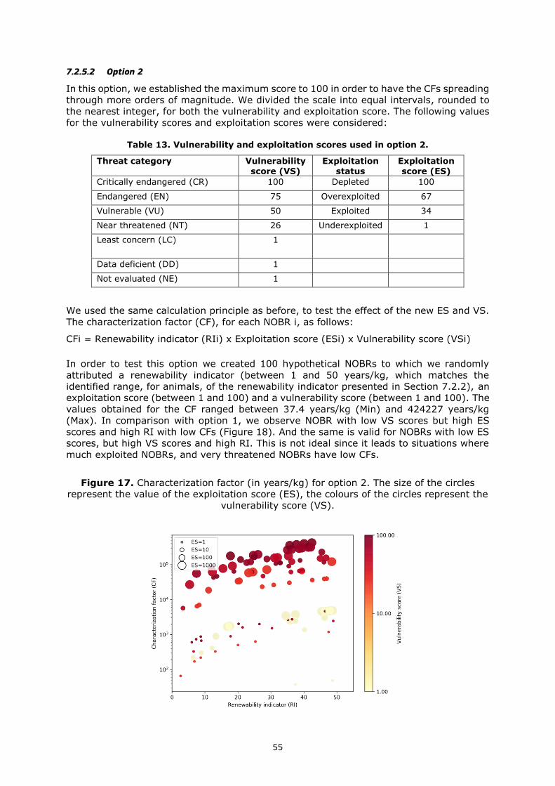
55

7.2.5.2 Option 2

In this option, we established the maximum score to 100 in order to have the CFs spreading

through more orders of magnitude. We divided the scale into equal intervals, rounded to

the nearest integer, for both the vulnerability and exploitation score. The following values

for the vulnerability scores and exploitation scores were considered:


Threat category Vulnerability score (VS)

Exploitation status

Exploitation score (ES)







Not evaluated (NE) 1

We used the same calculation principle as before, to test the effect of the new ES and VS.

The characterization factor (CF), for each NOBR i, as follows:


In order to test this option we created 100 hypothetical NOBRs to which we randomly



exploitation score (between 1 and 100) and a vulnerability score (between 1 and 100). The

values obtained for the CF ranged between 37.4 years/kg (Min) and 424227 years/kg

(Max). In comparison with option 1, we observe NOBR with low VS scores but high ES

scores and high RI with low CFs (Figure 18). And the same is valid for NOBRs with low ES

scores, but high VS scores and high RI. This is not ideal since it leads to situations where

much exploited NOBRs, and very threatened NOBRs have low CFs.

Figure 17. Characterization factor (in years/kg) for option 2. The size of the circles



56

7.2.5.3 Option 3

In this option, we adopted a logarithmic approach in attributing the values to the

vulnerability and exploitation scores:


Threat category Vulnerability score (VS)

Exploitation status

Exploitation score (ES)







Not evaluated (NE) 1-

We used the same model as before, to test the effect of the new ES and VS. The

characterization factor (CF), for each NOBR i, as follows:


In order to test this option we created 100 hypothetical NOBRs to which we randomly



exploitation score (between 1 and 10000) and vulnerability score (between 1 and 1000).

The values obtained for the CF ranged between 26.2 years/kg (Min) and 4.2E8 years/kg

(Max). In this option we observe that NOBR with low VS and low ES typically have lower

CFs, for NOBR with the same VS and ES the differences in CFs are given by the RI (higher

RI, higher CF) (Figure 18). The large range of CF values might also improve the

discriminating power of the characterization step. Indeed, NOBR with high VS and ES,

could be easily identified even if their mass in the inventory are relatively limited.

Figure 18. Characterization factors (in years/kg) for option 3. The size of the circles



57

7.2.5.4 Option 4

In this option we consider the same values of the exploitation and vulnerability scores as

in option 1 (Table 6).

However, we built a different model with the aim of systematically increase the CFs of

species with high VS and high ES.

We computed the characterization factor (CF), for each NOBR i, as follows:

CF𝑖 = RI𝑖 + ΔRI (1

2

𝑉𝑆𝑖 − 𝑉𝑆𝑀𝐼𝑁

𝑉𝑆𝑀𝐴𝑋 − 𝑉𝑆𝑀𝐼𝑁

+1

2

𝐸𝑆𝑖 − 𝐸𝑆𝑀𝐼𝑁

𝐸𝑆𝑀𝐴𝑋 − 𝐸𝑆𝑀𝐼𝑁

)

In this case, we established ΔRI = RIMAX, the maximum value of the renewability indicator

from our sample. However, other choices can be made, for example establish the value of

ΔRI in relation to a reference species. In this approach, as in the previous ones, if VS and

ES are equal to 1, then the CF= RI. This modelling approach also allows to establish

different weights for VS and ES

The values obtained for the CF ranged between 8.7 years/kg (Min) and 91.3 years/kg

(Max). In this case, CF values are more homogenously spread across the CF range (Figure

19). With this option, we observe that NOBRs with high ES and high VS having higher CFs,

whereas NOBRs with low ES and low VS have consistently lower values However, here the

CF values do not span over several orders of magnitude which is reduces their

discriminatory power.

Figure 19. Characterization factors (in years/kg) for option 4. The size of the circles



58

7.3 Operationalizing the impact assessment of natural biotic resources: fish case

study

In this section, we present an operationalization of the impact assessment framework, for

naturally occurring biotic resources (NOBRs). We start with the elementary flows list from

Crenna et al. (2018), and focus on fish species, since this the NOBR for which we were

able to find systematic information regarding the status of exploitation. We compiled

information on exploitation status and vulnerability for 42 fish species (Annex 6). The

following sources were used to determine the exploitation level of the fish stocks:

International Council for the Exploration of the Sea (ICES) Stock Assessment

Graphs (http://standardgraphs.ices.dk/stockList.aspx)

International Commission for the Conservation of Atlantic Tunas (ICCAT) Stock

Assessment (https://www.iccat.int/en/assess.html)

Fisheries and Resources Monitoring System (FIRMS-FAO) Marine Resource Fact

Sheets (http://firms.fao.org/firms/resource/search/en)

General Fisheries Commission for the Mediterranean (GFCM-FAO) Stock

Assessment Forms (http://www.fao.org/gfcm/data/safs)

Scientific, Technical and Economic Committee for Fisheries (STECF-European

Commission) Stock Assessment Database in the Mediterranean and Black Sea

(https://stecf.jrc.ec.europa.eu/web/stecf/dd/medbs/sambs)

The vulnerability scores, as explained in Subsection 7.2.4, were determined using IUCN’s

Red List of Threatened Species (IUCN, 2019).

The exploitation status of fish stocks is determined for specific populations and

geographical regions, therefore the exploitation scores are regionalized (the regional detail

varies between species). We determined 87 exploitation scores for 42 fish species (Annex

6).

7.3.1 Characterization factors for fish species taking into account renewability and

exploitation level.

We computed the characterization factors (CFs), according to option 1, option 3 and option

4 described in Section 7.2.5 (values presented in Annex 6). Option 2 was excluded from

this analysis as it was the least promising option due to the fact that, for this option, the

lower characterisation factors were obtained for species with VS score.

The CFs computed with option 1 (see Figure 20 and Annex 6), ranged from 1.3 years/kg

(Hemitaurichthys polylepis to 451 years/kg (Squalus acanthias). The range of values spans

only two orders of magnitude, this can allow for the impacts to be mostly determined by

the inventory rather than the characterization factors (for example, a very endangered and

exploited species with a high characterization factor but inventoried in low quantities would

have a lower impact that a not endangered nor exploited species inventoried in large

quantities). The maximum value found is quite distant from the other values (see Figure

20). The highest value is found for a species that is highly exploited (size of the circles),

but that is at an intermediate level of extinction risk (colours from yellow to red). Species

with an intermediate level of exploitation but highly endangered show a much lower

characterization factor (Anguilla anguilla and Thunnus maccoyii).

The characterization factor computed with option 3 (see Figure 21 and Annex 6), ranged

from 1.3 years/kg (Hemitaurichthys polylepis to 9250000 years/kg (Anguilla Anguilla) to).

http://standardgraphs.ices.dk/stockList.aspx

https://www.iccat.int/en/assess.html

http://firms.fao.org/firms/resource/search/en

http://www.fao.org/gfcm/data/safs

https://stecf.jrc.ec.europa.eu/web/stecf/dd/medbs/sambs

59

The high range of values allows for species not exploited in large quantities to have high

impacts. Species with a high extinction risk and an intermediate exploitation level have the

higher characterization factors (Anguilla anguilla and Thunnus maccoyii) (see Figure 21).

With option 3, the characterization factors appear to be well differentiated, higher values

for species with higher extinction risks and exploitation levels, and lower values for species

with lower extinction risks and lower exploitation levels. Also species with higher

renewability times have higher characterization factors.

Figure 20. Characterization factors for fish, computed following option 1, described in

Section 7.2.5.1. The size of the circles represent the value of the exploitation score (ES),

the colours of the circles represent the vulnerability score (VS).




Finally, the characterization factors computed following option 4 (see Figure 22 and Annex

6) showed similar patterns to those observed with option 3. However the range of values

was much lower, spanning from 15.4 years/kg (Hemitaurichthys polylepis) and 110.9

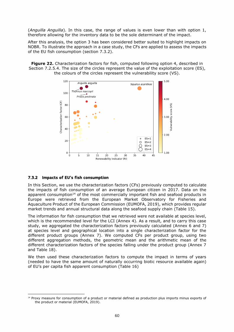
60

(Anguilla Anguilla). In this case, the range of values is even lower than with option 1,

therefore allowing for the inventory data to be the sole determinant of the impact.

After this analysis, the option 3 has been considered better suited to highlight impacts on

NOBR. To illustrate the approach in a case study, the CFs are applied to assess the impacts

of the EU fish consumption (section 7.3.2).




7.3.2 Impacts of EU’s fish consumption

In this Section, we use the characterization factors (CFs) previously computed to calculate

the impacts of fish consumption of an average European citizen in 2017. Data on the

apparent consumption14 of the most commercially important fish and seafood products in

Europe were retrieved from the European Market Observatory for Fisheries and

Aquaculture Product of the European Commission (EUMOFA, 2019), which provides regular

market trends and annual structural data along the seafood supply chain (Table 15).

The information for fish consumption that we retrieved were not available at species level,

which is the recommended level for the LCI (Annex 4). As a result, and to carry this case

study, we aggregated the characterization factors previously calculated (Annex 6 and 7)

at species level and geographical location into a single characterization factor for the

different product groups (Annex 7). We computed CFs per product group, using two

different aggregation methods, the geometric mean and the arithmetic mean of the

different characterization factors of the species falling under the product group (Annex 7

and Table 18).

We then used these characterization factors to compute the impact in terms of years

(needed to have the same amount of naturally occurring biotic resource available again)

of EU’s per capita fish apparent consumption (Table 16)

14 Proxy measure for consumption of a product or material defined as production plus imports minus exports of

the product or material (EUMOFA, 2019).

61

Table 15. Apparent consumption of the most important fish and seafood products in

Europe in 2017. Minor species are grouped in the “others” category. Apparent consumption is defined as production plus imports minus exports of the product. The

lines shaded in green indicate the products groups to which we can provide a characterization factor. Adapted from EUMOFA (2019).

Products

Per capita consumption

(kg, live weight

equivalent)

% wild % farmed


(kg from wild)


(kg from farmed)

Tuna1 3.07 99.17 0.83 3.045 0.025

Cod 2.31 99.97 0.03 2.309 0.001

Salmon 2.24 0.05 99.95 0.001 2.239

Alaska pollock

1.59 100 0 1.590 0.000

Shrimps 1.51 50.87 49.13 0.768 0.742

Mussel 1.28 8.44 91.56 0.108 1.172

Herring 1.18 100 0 1.180 0.000

Hake 0.94 100 0 0.940 0.000

Squid 0.67 100 0 0.670 0.000

Mackerel 0.65 100 0 0.650 0.000

Sardine 0.58 100 0 0.580 0.000

Surimi2 0.53 100 0 0.530 0.000

Trout 0.42 0.21 99.79 0.001 0.419

Sprat (= Brisling)

0.37 100 0 0.370 0.000

Freshwater catfish

0.36 0.3 99.7 0.001 0.359

Other 6.65 79.09 20.91 5.259 1.391

Total 24.35 73.9 18.002 6.347 1 This is a multispecies group considering the following species: skipjack, yellowfin, albacore, bigeye, bluefin and miscellaneous.

2 Surimi is made from wild-caught species (mainly Alaska pollock, blue whiting, blue grenadier, and Pacific hake).

Table 16. Characterization factors (CFs) for product groups, aggregated using geometric mean and arithmetic mean, and impact (in years) of Europe’s apparent fish consumption

in 2017.

Products

CFs, geometric mean,

years/kg (following option 3)

CFs, arithmetic mean,

years/kg (following option 3)


(kg from wild)

Impact in years, with geometric

mean

Impact in years, with geometric

mean

Tuna1 260.15 358556 3.045 792.02 1091803.02

Cod 2429.27 13541 2.309 5609.92 31266.17

Salmon 29.00 146.45 0.001 0.03 0.146

Herring 23.04 96.86 1.180 27.18 114.30

Sardine 197.57 246.5 0.580 114.59 142.97

Trout 13.00 13.00 0.001 0.01 0.013

Total 7.116 6543.76 1123326.61

1 This is a multispecies group considering the following species: skipjack, yellowfin, albacore, bigeye, bluefin and miscellaneous.

62

The impact assessment framework described in this report allows determining the impacts

of exploitation of NOBR in terms of number of years necessary to have the same amount

of resource available in nature once again. In this case study we show that the consumption

of different species has very different impacts in terms of exploitation of NOBR. We present

two sets of results, one using a geometric mean to aggregate the CFs at the species level,

per product group, and another one using an arithmetic mean. Using the geometric mean,

our results show that while tuna is the species most consumed per capita in the EU, it is

the consumption of cod that has a higher impact.

Bluefin tunas are more endangered than other tuna’s species, and then cod. Our results,

show that great care needs to be taken, when aggregating CFs per species groups, since

this will greatly influence the results. If data would be available, performing the same

analysis at the species level (for tuna) would probably yield different results. Hence, the

recommendation is to apply the CFs at species level when assessing NOBR.

63

8 Conclusions

One of the most widely applied approaches to account for the impacts associated with

mineral and metal resource use in the Life Cycle Impact Assessment (LCIA) step relies on

the concept of “depletion”. This is also the underlying concept of the Abiotic Depletion

Potential (ADP) currently recommended in the EF methods. The extraction of a resource

from the Earth’s crust implies the reduction of the corresponding geological stocks, and is

considered to subsequently contribute to this resource depletion. While the ADP is one of

the most commonly used methods, it has limitations that were broadly discussed within

the scientific community in the past years. In the latest years, methods based on the

concept of dissipation have been seen as more promising. In this respect, a resource

indicator should be designed to allow to properly inform the decision makers: meaningful

information, which may also embed economic aspects, may be preferred to purely

environmental considerations.

The concept of resource dissipation has not yet been practically applied in LCA, therefore

different researchers have different understanding of what dissipation actually is. In this

report, a definition of resource dissipation is provided, building on a thorough literature

analysis:

Dissipative flows of abiotic resources are flows to sinks or stocks that are not accessible to

future users due to different constraints. These constraints prevent humans to make use

of the function(s) that the resources could have in the technosphere. The distinction

between dissipative and non-dissipative flows of resources may depend on technological

and economic factors, which can change over time.

This definition takes into account different aspects: i) abiotic resources in a large sense,

that is including both natural (or “primary”) resources extracted from the ground and

secondary resources produced through recycling operations; ii) the function a resource

may hold, iii) the temporal dimension, therefore making the timeframe a key feature of

any approach aimed at quantifying resource dissipation; iv)“flows to sinks or stocks”,

therefore, implicitly encompassing flows to the three compartments most commonly

distinguished in the literature: environment, products in use (non-functional recycling) and

waste disposal facilities; v) technological and economic factors as potential determinants

to discriminate “dissipative flows” from “non-dissipative flows”.

In this report an approach to account for resource dissipation at LCI and LCIA level has

been developed and applied to case studies.

Regarding the LCI step, the approach described in this report the following flows of

resources at the unit process level are considered inaccessible to future users in a 25-year

timeframe: i) any emission of mineral or metal resource to the environment (air, water

and soil), ii) any flow of mineral and metal resource, as such or embodied in a waste

fraction, sent to a final waste disposal facility, iii) any flow of mineral and metal resource,

as such or embodied in a waste fraction, sent to recovery and subsequently recovered with

low-functionality (including non-functional recycling). This reduction in functionality should

be associated with an impossibility to recover the original, or any significant, value of the

resource later in the life cycle.

When considering the LCIA step it was suggested an approach based on the economic

value of resources: the target of a circular and resource efficient economy is linked to

maintaining the “value” of products, materials and resources for as long as possible. In

this perspective, the price of resources could be considered as a simplified ‘proxy’ for the

complex utility that resources have for humans, and it could be used to address the impact

of resource dissipation. It is noteworthy that this approach could be applied both with

respect to resources extracted, as currently commonly considered in LCI datasets, and

resources dissipated. Furthermore, it could be valuable exploring how the price-based

impact assessment approach could be extended to abiotic resources as a whole, that is

including not only mineral and metal resources but also fossil resources.

64

At this point in time, the approach proposed in this report still cannot be seen as a fully

applicable method, so it cannot replace or expand the current recommendation in an EF

context (i.e. the ADP). Therefore, it should be used by researchers as a basis to develop

methods that are fully applicable and potentially used in an Environmental Footprint

context. At the end of 2019 the SUPRIM project published its final deliverables: it is also

recommended that researchers look into the framework provided in this project, to ensure

consistency between the problem at stake and the method developed.

Regarding biotic resources, the concept of dissipation could be in principle applied to them

as well, but it is implementation still requires in depth research and discussion. However,

the main challenge addressed in this report is related to the characterization of the impacts

of overexploitation of naturally occurring biotic resources. Here, we propose a set of

characterization factors which account for the renewability rate of the resource as well as

the vulnerability and the current exploitation level. These three elements are those

hampering a steady provision of biotic resource from the wild. Further research is needed

to complete the set of characterization factors for all the species with a commercial value,

in order to allow practitioners to apply the approach to different biotic resources: plants,

animals, fish etc.

65

References

- Alvarenga, R.A.F., Dewulf, J., Van Langenhove, H., Huijbregts, M.A.J., 2013.

Exergy-based accounting for land as a natural resource in life cycle assessment.

International Journal of Life Cycle Assessment 18, 939–947.

https://doi.org/10.1007/s11367-013-0555-7.

- Ardente, F., Beylot, A., Zampori, L., 2019. Towards the accounting of resource

dissipation in LCA. XIII Conference of Rete Italiana LCA, Rome, 14-15 June 2019.

Proceedings available at: http://www.reteitalianalca.it/attivita/organizzazione-

convegni/Convegno_Rete_Italiana_LCA_Roma_2019/atti-convegno-2019

- Bach, V., Berger, M., Finogenova, N. and Finkbeiner, M., 2017. Assessing the

availability of terrestrial biotic materials in product systems (BIRD). Sustainability,

9(1), 137. https://doi.org/10.3390/su9010137.

- Berger, M., Sonderegger, T., Alvarenga, R., Bach, V., Cimprich, A., Dewulf, J.,

Frischknecht, R., Guinée, J., et al., 2020. Mineral resources in Life Cycle Impact

Assessment – Part II: Recommendations on application-dependent use of existing

methods and on future method development needs. International Journal of Life

Cycle Assessment 1-16, https://doi.org/10.1007/s11367-020-01737-5.

- Beylot, A., Ardente, F., Sala, S., Zampori, L., 2020. Accounting for the dissipation

of abiotic resources in LCA: status, key challenges and potential way forward.

Resources, Conservation and Recycling 157, 104748.

https://doi.org/10.1016/j.resconrec.2020.104748.

- Beylot, A., Muller, S., Descat, M., Ménard, Y., Villeneuve, J., 2018. Life cycle

assessment of the French municipal solid waste incineration sector. Waste

Management 80, 144–53. https://doi.org/10.1016/j.wasman.2018.08.037.

- Boustead, I., 2005. Polyvinylchloride (PVC) (Bulk Polymerisation). Eco-profiles of

the European Plastics Industry. The European Council of Vinyl Manufacturers.

- Bunge, R., 2015. Recovery of metals from waste incinerator bottom ash. Report of

Institut für Umwelt und Verfahrenstechnik UMTEC. 2015. Available at: https://www.umtec.ch/fileadmin/user_upload/umtec.hsr.ch/Dokumente/News/1504_Metals

_from_MWIBA__R._Bunge.pdf (Accessed November 2019).

- Charpentier Poncelet, A., Loubet, P., Laratte, B., Muller, S., Villeneuve, J.,

Sonnemann, G., 2019. A necessary step forward for proper non-energetic abiotic

resource use consideration in life cycle assessment: The functional dissipation

approach using dynamic material flow analysis data. Resources, Conservation and

Recycling 151, 104449. https://doi.org/10.1016/j.resconrec.2019.104449.

- Classen, M., Althaus, H.-J., Blaser, S., Tuchschmid, M., Jungbluth, N., Doka, G.,

Faist Emmenegger, M., Scharnhorst, W., 2009. Life Cycle Inventories of metals.

Final report ecoinvent data v2.1 No.10. EMPA Dübendorf, Swiss Centre for Life Cycle

Inventories, Dübendorf, CH.

- CML, 2016. CML-IA Characterisation Factors. Leiden University. https://www.universiteitleiden.nl/en/research/research-output/science/cml-ia-

characterisation-factors (Accessed October 2019).

- Crenna, E., Sozzo, S., Sala, S., 2018. Natural biotic resources in LCA: Towards an

impact assessment model for sustainable supply chain management. Journal of

Cleaner Production 172, 3669–3684. https://doi.org/10.1016/j.jclepro.2017.07.208.

- Cusano, G., Rodrigo Gonzalo, M., Farrell, F., Remus, R., Roudier, S., Delgado

Sancho L., 2017. Best Available Techniques (BAT) Reference Document for the main

Non-Ferrous Metals Industries, EUR 28648 EN. https://doi.org/10.2760/8224.

- Dewulf, J., Bösch, M.E., Meester, B.D., Vorst, G.V. der, Langenhove, H.V., Hellweg,

S., Huijbregts, M.A.J., 2007. Cumulative Energy Extraction from the Natural

https://doi.org/10.1007/s11367-013-0555-7

http://www.reteitalianalca.it/attivita/organizzazione-convegni/Convegno_Rete_Italiana_LCA_Roma_2019/atti-convegno-2019

http://www.reteitalianalca.it/attivita/organizzazione-convegni/Convegno_Rete_Italiana_LCA_Roma_2019/atti-convegno-2019

https://doi.org/10.3390/su9010137

https://doi.org/10.1007/s11367-020-01737-5

https://doi.org/10.1016/j.resconrec.2020.104748

https://doi.org/10.1016/j.wasman.2018.08.037

https://www.umtec.ch/fileadmin/user_upload/umtec.hsr.ch/Dokumente/News/1504_Metals_from_MWIBA__R._Bunge.pdf

https://www.umtec.ch/fileadmin/user_upload/umtec.hsr.ch/Dokumente/News/1504_Metals_from_MWIBA__R._Bunge.pdf

https://doi.org/10.1016/j.resconrec.2019.104449

https://www.universiteitleiden.nl/en/research/research-output/science/cml-ia-characterisation-factors

https://www.universiteitleiden.nl/en/research/research-output/science/cml-ia-characterisation-factors

https://doi.org/10.1016/j.jclepro.2017.07.208

https://doi.org/10.2760/8224

66

Environment (CEENE): a comprehensive Life Cycle Impact Assessment method for

resource accounting. Environmental Science & Technology 41, 8477–8483.

https://doi.org/10.1021/es0711415.

- Dewulf, J., Mancini, L., Blengini, G., Sala, S., Latunussa, C., Pennington, D., 2015a.

Towards an overall analytical framework for the integrated Sustainability

Assessment of the production and supply of raw materials and primary energy

carriers. Journal of Industrial ecology 19(6), 963-977.

https://doi.org/10.1111/jiec.12289.

- Dewulf, J., Benini, L., Mancini, L., Sala, S., Blengini, G., Ardente, F., Recchioni, M.,

Maes, J., Pant, R., Pennington, D., 2015b. Rethinking the Area of Protection ‘Natural

Resources’ in Life Cycle Assessment. Environmental Science & Technology 49(9),

5310–5317. https://doi.org/10.1021/acs.est.5b00734.

- Doka, G., 2008a. Life Cycle Inventory Data of Mining Waste: Emissions from Sulfidic

Tailings Disposal. Gabor Doka Zürich.

- Doka, G., 2008b. Calculation Tool for waste disposal in Municipal Solid Waste

Incinerators MSWI - For ecoinvent v2.1.

- Drielsma, J.A., Russell-Vaccari, A.J., Drnek, T., Brady, T., Weihed, P., Mistry, M.,

Perez Simbor, L., 2016. Mineral resources in life cycle impact assessment - Defining

the path forward. International Journal of Life Cycle Assessment 21, 85–105. https://doi.org/10.1007/s11367-015-0991-7.

- Drielsma, J., Sochorová, V., 2019. SUstainable management of PRIMary raw

materials through a better approach in Life Cycle Sustainability Assessment

(SUPRIM). Newsletter, May 2019. Available at:

http://www.euromines.org/files/suprim-newsletter_210x297mm_e_final_0.pdf (Accessed

November 2019).

- EC, (European Commission). 2008. Communication from the Commission to the

European Parliament and the Council - The raw materials initiative: meeting our

critical needs for growth and jobs in Europe. SEC(2008) 2741.

- EC, (European Commission). 2013a. Commission Recommendation (2013/179/EU)

of 9 April 2013 on the use of common methods to measure and communicate the

life cycle environmental performance of products and organisations. Official Journal

of the European Communities 56, L124.

https://doi.org/10.3000/19770677.L_2013.124.eng.

- EC, (European Commission). 2013b. Communication from the Commission to the

European Parliament and the council. Building the Single Market for Green Products.

Facilitating better information on the environmental performance of products and

organisations. COM/2013/196.


European Parliament, the Council, the European Economic and Social Committee

and the Committee of the Regions. Closing the loop - An EU action plan for the

Circular Economy. COM/2015/0614.

- EC, (European Commission). 2017. Study on the review of the list of Critical Raw

Materials Critical Raw Materials Factsheets. Available at:

https://publications.europa.eu/s/naRu (Accessed November 2019).

- EC, (European Commission). 2018a. The Environmental Footprint Pilots. Last

updated: 08/06/2018. Available at:

https://ec.europa.eu/environment/eussd/smgp/ef_pilots.htm (Accessed April 2019).

- EC, (European Commission). 2018b. Organisation Environmental Footprint Sector

Rules – Copper production. Version number 3.0. Date of publication: 25 April 2018.

Available at:

https://doi.org/10.1021/es0711415

https://doi.org/10.1111/jiec.12289

https://doi.org/10.1021/acs.est.5b00734

https://doi.org/10.1007/s11367-015-0991-7

http://www.euromines.org/files/suprim-newsletter_210x297mm_e_final_0.pdf

https://doi.org/10.3000/19770677.L_2013.124.eng

https://publications.europa.eu/s/naRu

https://ec.europa.eu/environment/eussd/smgp/ef_pilots.htm

67

http://ec.europa.eu/environment/eussd/smgp/documents/OEFSR_Copper.pdf (Accessed

April 2019).

- EC, (European Commission) 2006. Communication from the Commission to the

European Parliament, the Council, the European Economic and Social Committee

and the Committee of the Regions. Thematic Strategy for Soil Protection

(SEC(2006)620, SEC(2006)1165). European Commission, Brussels.

- EC-JRC, (European Commission - Joint Research Centre). 2010. International

Reference Life Cycle Data System (ILCD) Handbook – General guide for Life Cycle

Assessment - Detailed guidance. First edition March 2010. EUR 24708 EN.

Luxembourg. Publications Office of the European Union, 2010.

- EC-JRC, (European Commission - Joint Research Centre). 2011. ILCD Handbook:

Recommendations for Life Cycle Impact Assessment in the European context.

https://doi.org/10.278/33030.

- ecoinvent. 2019. The ecoinvent Database. Available at:

https://www.ecoinvent.org/home.html (Accessed November 2019).

- EEA, 2017. Forest: growing stock, increment and fellings. Forest: growing stock,

increment and fellings. Available at: https://www.eea.europa.eu/data-and-

maps/indicators/forest-growing-stock-increment-and-fellings-3/assessment (Accessed

November 2019).

- Emanuelsson, A., Ziegler, F., Pihl, L., Sköld, M., Sonesson, U., 2014. Accounting for

overfishing in life cycle assessment: new impact categories for biotic resource use.

International Journal of Life Cycle Assessment 19, 1156–1168. https://doi.org/10.1007/s11367-013-0684-z.

- EUMOFA (European Market Observatory for Fisheries and Aquaculture Product),

2016. The EU fish market. 2016 Edition. Directorate-General for Maritime Affairs

and Fisheries of the European Commission. Available at: https://www.eumofa.eu

(Accessed November 2017).

- EUROSTAT, 2019. Key European Statistics: Waste Electrical and Electronic

Equipment (WEEE). Available at: https://ec.europa.eu/eurostat/web/waste/key-waste-

streams/weee (Accessed October 2019).

- FAO, 2011. Review of the state of world marine fishery resources (No. 569), FAO

Fisheries and Aquaculture Technical paper. FAO, Rome.

- FAO, 2016a. Global Statistical Collections on Fisheries and Aquaculture. Available

at: http://www.fao.org/fishery/statistics/en (Accessed March 2016).

- FAO, 2016b. FAOSTAT Forestry online database. Available at:

http://www.fao.org/forestry/statistics/84922/en/ (Accessed March 2016).

- FAO, 2018. The State of World Fisheries and Aquaculture 2018 - Meeting the

sustainable development goals. FAO, Rome.

- Federation of Associations for Hunting and Conservation of the European Union

(FACE), 2016. Artemis: the Information Portal of Huntable Species in Europe.

Available at: http://www.artemis-face.eu/about-the-database (Accessed March 2016).

- Finnveden, G., Hauschild, M.Z., Ekvall, T., Guinée, J., Heijungs, R., Hellweg, S.,

Koehler, A., Pennington, D., Suh, S., 2009. Recent developments in Life Cycle

Assessment. Journal of Environmental Management 91, 1–21.

https://doi.org/10.1016/j.jenvman.2009.06.018.

- Frischknecht, R., 2014. Impact assessment of abiotic resources: the role of

borrowing and dissipative resource use. LCA Forum 55, April 11, 2014, ETH Zürich.

Available at: http://www.lcaforum.ch/portals/0/df55/DF55-05%20Frischknecht.pdf

(Accessed November 2019).

http://ec.europa.eu/environment/eussd/smgp/documents/OEFSR_Copper.pdf

https://doi.org/10.278/33030

https://www.ecoinvent.org/home.html

https://www.eea.europa.eu/data-and-maps/indicators/forest-growing-stock-increment-and-fellings-3/assessment

https://www.eea.europa.eu/data-and-maps/indicators/forest-growing-stock-increment-and-fellings-3/assessment

https://doi.org/10.1007/s11367-013-0684-z

https://www.eumofa.eu/

https://ec.europa.eu/eurostat/web/waste/key-waste-streams/weee

https://ec.europa.eu/eurostat/web/waste/key-waste-streams/weee

http://www.fao.org/fishery/statistics/en

https://www.fao.org/forestry/statistics/84922/en/

http://www.artemis-face.eu/about-the-database

https://doi.org/10.1016/j.jenvman.2009.06.018

http://www.lcaforum.ch/portals/0/df55/DF55-05%20Frischknecht.pdf

68

- Gilbert, M., Patrick, S., 2017. Poly(Vinyl Chloride). in Brydson's Plastics Materials

(Eighth Edition), 2017.

- Guinée, J.B., Gorée, M., Heijungs, R., Huppes, G., Kleijn, R., de Koning, A., van

Oers, L., Wegener Sleeswijk, A., Suh, S., Udo de Haes, H.A., et al., 2002. Handbook

on Life Cycle Assessment: Operational Guide to the ISO Standards. Kluwer

Academic Publisher. Dordrecht, The Netherlands, 2002.

- Guinée, J.B., Heijungs, R., 1995. A proposal for the definition of resource

equivalency factors for use in product life-cycle assessment. Environmental

Toxicology and Chemistry 14, 917–925. https://doi.org/10.1002/etc.5620140525.

- Hélias, A., Langlois, J., Fréon, P., 2018. Fisheries in life cycle assessment:

Operational factors for biotic resources depletion. Fish and Fisheries 19, 951–963. https://doi.org/10.1111/faf.12299.

- Harris, J., Green, J., Prawiradilaga, D., Giam, X., Giyanto, Hikmatullah, D., Putra,

C., Wilcove, D., 2015. Using market data and expert opinion to identify

overexploited species in the wild bird trade. Biological Conservation 187, 51–60.

https://doi.org/10.1016/j.biocon.2015.04.009.

- Heywood, V., 1999. Use and potential of wild plants in farm households (No. 15).

Food and Agriculture Organization of the United Nations. Rome, Italy.

- IPBES, 2019. Summary for policymakers of the global assessment report on

biodiversity and ecosystem services of the Intergovernmental Science-Policy

Platform on Biodiversity and Ecosystem Services. IPBES secretariat, Bonn,

Germany.

- IRP, 2019. Global Resources Outlook 2019: Natural resources for the future we

want. A Report of the International Resource Panel. United Nations Environment

Programme. Nairobi, Kenya.

- ISO 14040, 2006. Environmental Management – Life Cycle Assessment – Principles

and Framework. International Organization for Standardization, Geneva,

Switzerland.

- IUCN, 2001. IUCN Red List Categories and Criteria: Version 3.1. IUCN Species

Survival Commission. IUCN, Gland, Switzerland and Cambridge, UK.

- IUCN, 2016. The IUCN red list of threatened species. Available at:

https://www.iucnredlist.org/(Accessed March 2016).

- IUCN, 2019. The IUCN red list of threatened species. Available at:

https://www.iucnredlist.org/ (Accessed December 2019).

- Jonkers, N., Krop, H., van Ewijk, H., Leonards, P. E. G., 2016. Life cycle assessment

of flame retardants in an electronics application. International Journal of Life Cycle

Assessment 2016, 21(2), 146–161. https://doi.org/10.1007/s11367-015-0999-z.

- Klinglmair, M., Sala, S., Brandão, M., 2014. Assessing resource depletion in LCA: a

review of models and methodological issues. International Journal of Life Cycle

Assessment 19(3), 580-592. https://doi.org/10.1007/s11367-013-0650-9.

- Kuipers, S., 1997. Trade in Medicinal Plants. Medicinal Plants for Forest

Conservation and Healthcare, Non-Wood Forest Products. FAO, Rome, Italy.

- Langlois, J., Fréon, P., Delgenes, J.-P., Steyer, J.-P., Hélias, A., 2014. New methods

for impact assessment of biotic-resource depletion in life cycle assessment of

fisheries: theory and application. Journal of Cleaner Production 73, 63–71.

https://doi.org/10.1016/j.jclepro.2014.01.087.

- Laner, D., Zoboli, O., Rechberger, H., 2017. Statistical entropy analysis to evaluate

resource efficiency: phosphorus use in Austria. Ecological Indicicators 83, 232–242.

https://doi.org/10.1016/j.ecolind.2017.07.060.

https://doi.org/10.1002/etc.5620140525

https://doi.org/10.1111/faf.12299

https://doi.org/10.1016/j.biocon.2015.04.009

https://www.iucnredlist.org/

https://www.iucnredlist.org/

https://doi.org/10.1007/s11367-015-0999-z

https://doi.org/10.1007/s11367-013-0650-9


https://doi.org/10.1016/j.ecolind.2017.07.060

69

- Lassesson, H., Karlfeldt Fedje, K., Steenari, B. M., 2014. Leaching for recovery of

copper from municipal solid waste incineration fly ash: Influence of ash properties

and metal speciation. Waste Management & Research, 32(8), 755-762. https://doi.org/10.1177/0734242X14542147.

- Licht, C., Peiró, L.T., Villalba, G., 2015. Global substance flow analysis of gallium,

germanium, and indium. Quantification of extraction, uses, and dissipative losses

within their anthropogenic cycles. Journal of Industrial Ecology 19, 890–903. https://doi.org/10.1111/jiec.12287.

- Lifset, R.J., Eckelman, M.J., Harper, E.M., Hausfather, Z., Urbina, G., 2012. Metal

lost and found: dissipative uses and releases of copper in the United States 1975-

2000. Science of the Total Environment 417, 138-147.

https://doi.org/10.1016/j.scitotenv.2011.09.075.

- Mihajlović, E., Cvetanović, S., Đorđević, A., Krstić, I., Popović, D., 2010. PVC

Material Fire Retardants. Working and Living Environmental Protection 2010, 7(1),

1–11.

- O’Brien, M., Bringezu, S., 2017. What is a sustainable level of timber consumption

in the EU: Toward global and EU benchmarks for sustainable forest use.

Sustainability 9, 812. https://doi.org/10.3390/su9050812.

- Pereira, H.M., Navarro, L.M., Martins, I.S., 2012. Global biodiversity change: the

bad, the good, and the unknown. Annual Review of Environment and Resources 37,

25–50. https://doi.org/10.1146/annurev-environ-042911-093511.

- Plastics Europe, 2016. Vinyl chloride (VCM) and Polyvinyl chloride (PVC).

PlasticsEurope/The European Council of Vinyl Manufacturers (ECVM) May 2015 -

December 2016.

- PVC4Cables, 2017. The production of PVC cables: Past and future of the value chain

- Safety, Environment, Performance, Cost-Effectiveness. Available at:

https://www.pvc4cables.org/images/THE PRODUCTION OF PVC CABLES.pdf (Accessed

November 2019).

- Ricard, D., Minto, C., Jensen, O.P., Baum, J.K., 2012. Examining the knowledge

base and status of commercially exploited marine species with the RAM Legacy

Stock Assessment Database. Fish and Fisheries 13, 380–398.

https://doi.org/10.1111/j.1467-2979.2011.00435.x.

- Rodrigues, A., Pilgrim, J., Lamoreux, J., Hoffmann, M., Brooks, T., 2006. The Value

of the IUCN Red List for conservation. Trends in Ecology & Evolution 21, 71–76.

https://doi.org/10.1016/j.tree.2005.10.010.

- Rugani, B., Huijbregts, M.A.J., Mutel, C., Bastianoni, S., Hellweg, S., 2011. Solar

Energy Demand (SED) of commodity Life Cycles. Environmental Science &

Technology 45, 5426–5433. https://doi.org/10.1021/es103537f.

- Sala, S., Benini, L., Castellani, V., Vidal Legaz, B., De Laurentiis, V., Pant, R., 2019.

Suggestions for the update of the Environmental Footprint Life Cycle Impact

Assessment. Impacts due to resource use, water use, land use, and particulate

matter. EUR 28636 EN, Publications Office of the European Union, Luxembourg,

ISBN 978-92-79-69335-9, https://doi.org/10.2760/78072.

- Sala, S., Farioli, F., Zamagni, A., 2013a. Life cycle sustainability assessment in the

context of sustainability science progress (part 2). International Journal of Life Cycle

Assessment 18, 1686–1697. https://doi.org/10.1007/s11367-012-0509-5.

- Sala, S., Farioli, F., Zamagni, A., 2013b. Progress in sustainability science: lessons

learnt from current methodologies for sustainability assessment: Part 1.

International Journal of Life Cycle Assessment 18, 1653–1672. https://doi.org/10.1007/s11367-012-0508-6.

https://doi.org/10.1177%2F0734242X14542147


https://doi.org/10.1016/j.scitotenv.2011.09.075

https://doi.org/10.3390/su9050812

https://doi.org/10.1146/annurev-environ-042911-093511

https://www.pvc4cables.org/images/THE%20PRODUCTION%20OF%20PVC%20CABLES.pdf

https://doi.org/10.1111/j.1467-2979.2011.00435.x

https://doi.org/10.1016/j.tree.2005.10.010

https://doi.org/10.1021/es103537f

https://doi.org/10.2760/78072

https://doi.org/10.1007/s11367-012-0509-5

https://doi.org/10.1007/s11367-012-0508-6

70

- Saouter, E., Biganzoli, F., Ceriani, L., Versteeg, D., Crenna, E., Zampori, L., Sala,

S, Pant, R., 2018. Environmental Footprint: Update of Life Cycle Impact Assessment

Methods – Ecotoxicity freshwater, human toxicity cancer, and non-cancer. EUR

29495 EN, Publications Office of the European Union, Luxembourg, ISBN 978-92-

79-98182-1. https://doi.org/10.2760/178544.

- Schneider, L., Berger, M., Finkbeiner, M., 2011. The anthropogenic stock extended

abiotic depletion potential (AADP) as a new parameterisation to model the depletion

of abiotic resources. International Journal of Life Cycle Assessment 16(9), 929-936. https://doi.org/10.1007/s11367-011-0313-7.

- Schneider, L., Berger, M., Finkbeiner, M., 2015. Abiotic resource depletion in LCA—

background and update of the anthropogenic stock extended abiotic depletion

potential (AADP) model. International Journal of Life Cycle Assessment 20(5), 709-

721. https://doi.org/10.1007/s11367-015-0864-0.

- Schroeder, P., Anggraeni, K., Weber, U., 2019. The relevance of circular economy

practices to the sustainable development goals. Journal of Industrial Ecology 23 (1),

77-95.

- Schulp, C.J.E., Thuiller, W., Verburg, P.H., 2014. Wild food in Europe: A synthesis

of knowledge and data of terrestrial wild food as an ecosystem service. Ecological

Economics 105, 292–305. https://doi.org/10.1016/j.ecolecon.2014.06.018.

- Schulze, E.D., Körner, C., Law, B.E., Haberl, H., Luyssaert, S., 2012. Large-scale

bioenergy from additional harvest of forest biomass is neither sustainable nor

greenhouse gas neutral. Global Change Biology Bioenergy 4, 611–616.

https://doi.org/10.1111/j.1757-1707.2012.01169.x.

- Schwarz-Schampera, U., 2014. Antimony. Gunn, G. (Editor), Critical Metals

Handbook, John Wiley & Sons, 70–98.

- Simonson, M., Blomqvist, P., Boldizar, A., Möller, K., Rosell, L., Tullin, C., Stripple,

H., Sundqvist. J.O., 2000. Fire-LCA Model: TV Case Study. Swedish National Testing

and Research Institute, Fire Technology, SP Report 2000:13.

- Sonderegger, T., Dewulf, J., Drielsma, J., Fantke, P., Maia de Souza, D., Pfister, S.,

Stoessel, F., Verones, F., Vieira, M., Weidema, B.P., Hellweg, S., 2017. Towards

harmonizing natural resources as an area of protection in Life Cycle Impact

Assessment. International Journal of Life Cycle Assessment 22, 1912-1927.

https://doi.org/10.1007/s11367-017-1297-8.

- Sonderegger, T., Berger, M., Alvarenga, R., Bach, V., Cimprich, A., Dewulf, J.,

Frischknecht, R., Guniéè, J., Helbig, C., Huppertz, T., Jolliet, O., Motoshita, M.,

Northey, S., Peña, C.A., Rugani, B., Sahnoune, A., Schrijvers, D., Schulze, R.,

Sonneman, G., Valero, A., Weidema, B.P., Young, S.B., 2020. Mineral resources in

life cycle impact assessment part I: a review. International Journal of Life Cycle

Assessment, https://doi.org/10.1007/s11367-020-01736-6.

- STECF, 2018. 2018 Mediterranean Stock Assessments - Part 2 (Publications Office

of the European Union). Scientific, Technical and Economic Committee for Fisheries,

Luxembourg.

- Steen, B., 1999. A systematic approach to environmental priority strategies in

product development (EPS). Version 2000-general system characteristics (CPM

Report 1999:4). Chalmers University of Technology, Gothenburg, Sweden.

- Stewart, M., Weidema, B., 2005. A Consistent framework for assessing the impacts

from resource use. A focus on resource functionality. International Journal of Life

Cycle Assessment, 10(4), 240–247. https://doi.org/10.1065/lca2004.10.184.

- Taelman, S.E., De Meester, S., Schaubroeck, T., Sakshaug, E., Alvarenga, R.A.F.,

Dewulf, J., 2014. Accounting for the occupation of the marine environment as a

natural resource in life cycle assessment: An exergy based approach. Resources,

https://doi.org/10.2760/178544

https://doi.org/10.1007/s11367-011-0313-7

https://doi.org/10.1007/s11367-015-0864-0

https://doi.org/10.1016/j.ecolecon.2014.06.018

https://doi.org/10.1111/j.1757-1707.2012.01169.x

https://doi.org/10.1007/s11367-017-1297-8

https://doi.org/10.1007/s11367-020-01736-6

https://doi.org/10.1065/lca2004.10.184

71

Conservation and Recycling 91, 1–10.

https://doi.org/10.1016/j.resconrec.2014.07.009.

- Thiébaud, E., Hilty L., M., Schluep, M., Böni, H., W., Faulstich, M., 2018. Where do

our resources go? Indium, neodymium, and gold flows connected to the use of

electronic equipment in Switzerland. Sustainability 10, 2658.

https://doi.org/10.3390/su10082658.

- Tittensor, D.P., et al. 2014. A mid-term analysis of progress towards international

biodiversity targets. Science 346, 241–244. https://doi.org/10.1126/science.1257484.

- UNEP, 2011. Recycling Rates of Metals - A Status Report, A report of the Working

Group on the Global Metal Flows to the International Resource Panel.

- UNEP, 2013. Metal recycling: Opportunities, limits, infrastructure. A Report of the

Working Group on the Global Metal Flows to the International Resource Panel.

Reuter, M. A.; Hudson, C.; van Schaik, A.; Heiskanen, K.; Meskers, C.; Hagelüken,

C., 2013.

- United States Antimony Corporation (USAC), 2017. Antimony - Uses and

formulations. Available at: https://usantimony.com/uses_formulations.htm (Accessed

November 2019).

- Vadenbo, C., Rørbech, J., Haupt, M., Frischknecht, R., 2014. Abiotic resources: New

impact assessment approaches in view of resource efficiency and resource criticality

- 55th Discussion Forum on Life Cycle Assessment, Zurich, Switzerland, April 11,

2014. International Journal of Life Cycle Assessment 19(10), 1686. https://doi.org/10.1007/s11367-014-0784-4.

- Van Oers, L., de Koning, A., Guinée, J.B. and Huppes G., 2002. Abiotic resource

depletion in LCA. Road and Hydraulic Engineering Institute, Ministry of Transport

and Water, Amsterdam.

- Van Oers, L., Guinée, J., 2016. The Abiotic Depletion Potential: Background,

updates, and future. Resources 5(1), 16. https://doi.org/10.3390/resources5010016.

- Van Tichelen, P., Ectors, D., Stevens, M., Chung, L. W., Peeters, K., 2015.

Preparatory studies for product group in the ecodesign working plan 2012-2014:

Lot 8 - Power cables - Task 1-7 report. Final Report.

- Weidema, B.P., Bauer, C., Hischier, R., Mutel, C., Nemecek, T., Reinhard, J.,

Vadenbo, C.O., Wernet, G., 2013. Overview and methodology. Data quality

guideline for the ecoinvent database version 3. Ecoinvent Report 1(v3). St. Gallen:

The ecoinvent Centre.

- Yellishetty, M., Mudd, G. M., & Ranjith, P. G., 2011. The steel industry, abiotic

resource depletion and life cycle assessment: a real or perceived issue?. Journal of

Cleaner Production 19(1), 78-90. https://doi.org/10.1016/j.jclepro.2010.08.020.

- Zampori, L., Sala, S., 2017. Feasibility study to implement resource dissipation in

LCA. EUR 28994 EN, Publications Office of the European Union, Luxembourg, 2017,

ISBN 978-92-79-77238-2, https://doi.org/10.2760/869503.

- Zampori, L., Pant, R., 2019. Suggestions for updating the Product Environmental

Footprint (PEF) method, EUR 29682 EN, Publications Office of the European Union,

Luxembourg, 2019, ISBN 978-92-76- 00654-1, https://doi.org/10.2760/424613.

- Zhang, L., Li, J., Ding, X., 2014. Research of the properties of flame-retardant

flexible PVC. American Journal of Materials Research 1(1), 20-25.

- Zimmermann, T., 2017. Uncovering the fate of Critical Metals: Tracking dissipative

losses along the product Life Cycle. Journal of Industrial Ecology 21(5), 1198-1211. https://doi.org/10.1111/jiec.12492.

https://doi.org/10.1016/j.resconrec.2014.07.009

https://doi.org/10.3390/su10082658

https://doi.org/10.1126/science.1257484

https://usantimony.com/uses_formulations.htm

https://doi.org/10.1007/s11367-014-0784-4

https://doi.org/10.3390/resources5010016


https://doi.org/10.2760/869503

https://doi.org/10.2760/424613

72

List of abbreviations and definitions

ADP Abiotic Depletion Potential

ARD Abiotic Resource Dilution

ATO Antimony Trioxide

B Current Stock Biomass

BMSY Biomass Level that allows for Maximum Stock Growth

CF Characterization factors

CR Critically Endangered (IUCN Red List Category)

DD Data Deficient (IUCN Red List Category)

EDC Ethylene Dichloride

EEA European Environmental Agency

EEE Electrical and Electronic Equipment

EF Environmental footprint

EN Endangered (IUCN Red List Category)

EoL End-of-Life

ES Exploitation Score

EW Extinct in the wild

EX Extinct

F Current Fishing Effort

FAO Food and Agriculture Organization of the United Nations

FIRMS-FAO Fisheries and Resources Monitoring System of FAO

FMSY Fishing effort that produces Maximum Sustainable Yield

GFCM-FAO General Fisheries Commission for the Mediterranean of FAO

ICCAT International Commission for the Conservation of Atlantic Tunas

ICES International Council for the Exploration of the Sea

IOA Input-Output Analysis

IUCN International Union for Conservation of Nature

JRC Joint Research Centre

LC Least Concern (IUCN Red List Category)

LCA Life Cycle Assessment

LCI Life Cycle Inventory

LCIA Life Cycle Impact Assessment

LPY Lost Potential Yield

MFA Material Flow Analysis

MSY Maximum Sustainable Yield

NE Not Evaluated (IUCN Red List Category)

NMVOC Non Methane Volatile Organic Chemicals

NOBR Naturally Occurring Biotic Resources

NOx Nitrogen Oxides

NT Near Threatened (IUCN Red List Category)

PEF Product Environmental Footprint

PVC Polyvinyl chloride

RD Resource Dissipation

RI Renewability Indicator

RSE Relative Statistical Entropy

SDGs Sustainable Development Goals

SED Solar Energy Demand

SFA Substance Flow Analysis

STECF Scientific, Technical and Economic Committee for Fisheries of the

European Commission

UNEP - SETAC United Nations Environment and Society for Environmental

Toxicology and Chemistry

USGS United States Geological Survey

VS Vulnerability Score

VU Vulnerable (IUCN Red List Category)

73

Definiendum Definition

Characterisation

A step of the Impact assessment, in which the environmental interventions assigned qualitatively to a specific impact category (in classification) are quantified in terms of a common unit for that category, allowing aggregation into one figure of the indicator result (Guinée et al., 2002).

Characterisation factor

Factor derived from a characterisation model which is applied to convert an assigned life cycle inventory analysis result to the common unit of the impact category indicator (ISO 14040).

non-functional recycling

“collection of old metal scrap flowing into a large magnitude material stream, as a “tramp” or impurity elements”, representing the “loss of its function” according to the United Nations Environment Programme definition (UNEP, 2011)

low-functional recovery

“low-functional recovery” is considered to include “non-functional recycling” but also other cases of recovery that depart from recycling, for which the recovered material provides such a low function compared to its potential functions (and accordingly, value) that it should not be considered a resource (e.g. copper in slags used as a filler in construction).

74

List of figures

Figure 1. Impact of resource use: moving from resources extracted from the ecosphere,

to dissipative flows of resources along the life cycle of products and systems into three

main dissipation compartments: i) to the environment; ii) to final waste disposal facilities

and iii) to products in use in the technosphere. 19

Figure 2. Scheme describing the rationale for the identification of the three main compartments of dissipation ( i) environment, ii) final waste disposal facilities and iii) products in use in the technosphere) in our approach. The criteria are: time before resources can be considered accessible to future users, by compartment and as a function of the level of constraints. The time scale is purely illustrative and should be further explored. 19

Figure 3. Flows at the unit process level: general scheme (from EC-JRC; 2010) modified

to account for dissipative flows to three main compartments 21

Figure 4. Characterisation factors for resource dissipation (referred to kg of Antimony

equivalent) 28

Figure 5. Characterisation factors for resource dissipation (referred to kg of Gold

equivalent) 29

Figure 6. Characterisation factors for resource dissipation (referred to kg of Copper

equivalent) 30

Figure 7. System boundaries for the analysis of the cradle-to-gate primary production of

copper 32

Figure 8. Input and output resource flows associated with copper concentration, as

derived from the corresponding ecoinvent “global” dataset 34

Figure 9. Copper mining and concentration: representation of dissipative flows as

elementary flows (to air and water; i.e. to environment) and flows within the

technosphere (in tailings; i.e. in a final waste disposal facility), after economic allocation

35

Figure 10. Input and output resource flows associated with copper pyrometallurgy, as

derived from the corresponding ecoinvent “global” dataset 36

Figure 11. Pyrometallurgy: representation of dissipative flows as elementary flows (to

air and water; i.e. to environment) and technical flows (in slags used in construction; i.e.

in a product-in-use) 37

Figure 12. Contributions of dissipative flows to the total dissipation of resources in the

production of copper (% in mass terms) 37

Figure 13. Contributions of dissipative flows to the total impact associated with the

dissipation of resources in the production of copper (price-based impact assessment

approach) 38

Figure 14. System boundaries for the analysis of a flame-retarded PVC electrical cable

for EEE 41

Figure 15. Dissipative flows of resources in the production of virgin PVC (step 1 of the

case study). 44

Figure 16. Cause – effect chain of the impacts associated to the use of naturally

occurring biotic resources and the characterization of their availability. PDF stands for

potentially disappeared fraction of species. The full line indicates the characterisation

model developed in this report. Adapted from Crenna et al. (2018). 51

75

List of tables

Table 1. Relevance, suitability and applicability of the Abiotic Resource Dilution approach

to assess resource dissipation in LCA and EF (van Oers et al., 2016) 12

Table 2. Relevance, suitability and applicability of the “ultimate quality limit” and “backup

technology” concepts (Stewart and Weidema, 2005) to assess resource dissipation in LCA

13

Table 3. Relevance, suitability and applicability of the “Relative Statistical Entropy”

approach, so far applied in SFA and MFA (see e.g. Laner et al., 2017), to assess resource

dissipation in LCA 14

Table 4. Characterisation factors based on prices (average 50 years) and ADP (ultimate

reserves and reserve base) the prices of different resources 26

Table 5. Comparison with alternative approaches for inventory and impact assessment:

main contributions by unit processes and resources 40

Table 6. Detail of main assumptions and data sources for the life cycle inventory 43

Table 7. Detail of dissipative flows for the production of 1 kg of Electrical Cable in the

three compartments, for the three different EoL scenarios 45

Table 8. Impact assessment of dissipative flows for 1 kg of electrical cable (as kgSb €eq.) 46

Table 9. Impact assessment: contributions of the different dissipative flows 47

Table 10. Number of NOBRs identified per taxonomic category (for full list see Annex 4.).

50

Table 11. Definition of the Red List categories (IUCN, 2019; Rodrigues et al., 2006). 53

Table 12. Vulnerability and exploitation scores used in option 1. 54



Table 15. Apparent consumption of the most important fish and seafood products in

Europe in 2017. Minor species are grouped in the “others” category. Apparent

consumption is defined as production plus imports minus exports of the product. The

lines shaded in green indicate the products groups to which we can provide a

characterization factor. Adapted from EUMOFA (2019). 61

Table 16. Characterization factors (CFs) for product groups, aggregated using geomentric

mean and arithmentic mean, and impact (in years) of Europe’s apparent fish

consumption in 2017. 61

76

Annexes

Annex 1. Definitions for natural resources

An exhaustive review of the scientific literature for definitions of ‘natural resource’ is

probably not possible, due to the huge number of studies which refer to them in different

contexts and fields (e.g. environmental, economic and social sciences and laws). A list of

some significant definitions is presented in Table A.1.

Table A.1: Definitions for ‘natural resources’ (non-exhaustive list from the literature)

(from Ardente et al. 2019)

Definition and reference

A thing can be a use-value without being a value. This is the case whenever its utility

to man is not mediated through labour. Air, virgin soil, natural meadows, unplanted

forests, etc. fall into this category. (Marx, 1867)

Natural resources can be defined as materials occurring in nature used and transformed

by ecosystems and humans, as studied by ecology. (Odum, 1971)

Natural resources are natural assets (raw materials) occurring in nature that can be

used for economic production or consumption. (UN, 1997)

A resource is an essential input to the economic process. Resources may be material

or immaterial (e.g. information) and material resources may be of natural origin or

man-made. Services provided by nature (e.g. `assimilative capacity’) are also

sometimes called resources. (Ayres, 2000)

Natural resources are objects of nature which are extracted by man from nature and

taken as useful input to man-controlled processes, mostly economic processes. (Udo

de Haes et al., 2002)

Natural resources include both the raw materials necessary for most human activities

and the different environmental media, such as air, water and soil, which sustain life

on our planet. (EC, 2003)

Resources are the backbone of every economy and provide two basic functions – raw

materials for production of goods and services, and environmental services. (Mensah &

Carmago Castro, 2004)

Natural resources pertain to materials that are extracted, harvested, or otherwise

obtained from the environment for beneficial use by humans. (Bare and Gloria, 2006)

Natural resources can be defined as natural assets or endowments from which we

derive value (utility). A broad definition would include environmental assets such as

wilderness which, while they can be destroyed by human activity, do not have to be

consumed in order to have value. (Hatcher, 2008)

Natural resources are stocks of materials that exist in the natural environment that are

both scarce and economically useful in production or consumption, either in their raw

state or after a minimal amount of processing. (WTO, 2010)

Natural resources provide essential inputs to production […]. Natural resources are also

part of the ecosystems that support the provision of services such as climate regulation,

flood control, natural habitats, amenities and cultural services that are necessary to

develop man-made, human and social capital. (OECD, 2015)

Natural resources are the state’s environmental and ecological assets; the land, water,

plants and animals that sustain us and enhance our quality of life. (State of the Rhode

Island, 2015)

Natural resources are defined broadly as the means for human actions and basis of

human livelihoods provided by nature […]. They are extended by all ecosystem

functions of earth and solar system usable by humans or funding human well-being […]

and the extracted raw materials sub-categorised in biotic and abiotic materials. Their

https://www.marxists.org/archive/marx/works/download/pdf/Capital-Volume-I.pdf

https://www.worldcat.org/title/fundamentals-of-ecology/oclc/767691115#borrow

https://unstats.un.org/unsd/publication/SeriesF/SeriesF_67E.pdf

https://flora.insead.edu/fichiersti_wp/inseadwp2002/2002-118.pdf

https://www.setac.org/store/ViewProduct.aspx?id=1036212


https://eur-lex.europa.eu/LexUriServ/LexUriServ.do?uri=COM:2003:0572:FIN:EN:PDF

https://www.zef.de/fileadmin/downloads/forum/docprog/Termpapers/2004_3b_Mensah_Castro.pdf


https://pubs.acs.org/doi/abs/10.1021/es051639b

https://www.economicsnetwork.ac.uk/sites/default/files/Aaron%20Hatcher/NRE-Lecture-1.pdf

https://www.wto.org/english/res_e/publications_e/wtr10_e.htm

https://www.oecd.org/environment/waste/material-resources-productivity-and-the-environment-9789264190504-en.htm

http://www.planning.ri.gov/documents/comp_handbook/1_CompPlan101.pdf


77

Definition and reference

value for humanity as living resource-pools embedded in ecosystems or as single

resource units is given by provisioning, supporting, cultural and regulating ecosystem

- or resource-services. (Holzgreve, 2015)

Natural resources are any raw materials (matter or energy) which are not created by

humans but are available to sustain human activities. (Banai, 2016)

Natural resources are material and non-material assets occurring in nature that are at

some point in time deemed useful for humans. (Sonderegger et al., 2017)

Resources — including land, water, air and materials — are seen as parts of the natural

world that can be used in economic activities to produce goods and services. (IRP,

2017)

- Marx, K., 1867. Capital: A critique of political economy. Volume I Book one: The

Process of Production of Capital. Available at: https://www.marxists.org/archive/marx/works/download/pdf/Capital-Volume-I.pdf.

- Odum, P.E., Barrett, G.W., 1971. Fundamentals of ecology. Philadelphia, Saunders

1971, 5. Available at: https://www.worldcat.org/title/fundamentals-of-

ecology/oclc/767691115#borrow.

- UN, 1997. Glossary of environment statistics. Department for Economic and Social

Inormation and Policy Analysis, Statistic Division. United Nations, New York. Studies

in Methods F, 67. Available at: https://stats.oecd.org/glossary/detail.asp?ID=1740.

- Ayres, R.U., 2000. Resources, scarcity, technology and growth and the

environment. INSEAD, Working Papers, The Centre for the Management of

Environmental Resources. Available at:

https://flora.insead.edu/fichiersti_wp/inseadwp2002/2002-118.pdf.

- De Haes, H.U., Finnveden, G., Goedkoop, M., Hauschild, M., Hertwich, E.,

Hofstetter, P., Jolliet, O., Klöpffer, W., Krewitt, W., Lindeijer, E., Müller-Wenk, R.,

Olsen, S., Pennington, D., Potting, J., Steen, B., 2002. Life-Cycle Impact

Assessment: Striving towards best practice. SETAC Press Proceedings. Available at: https://www.setac.org/store/ViewProduct.aspx?id=1036212.


European Parliament and the council. Towards a thematic strategy on the

sustainable use of natural resources. COM/2003/572. Available at: https://eur-

lex.europa.eu/LexUriServ/LexUriServ.do?uri=COM:2003:0572:FIN:EN:PDF.

- Mensah, A.M., Camargo Castro, L., 2004. Sustainable resource use & sustainable

development: A contradiction?!. Zentrum fur Entwicklungsfourschung (ZEF), Center

for Development Research, University of Bonn. Available at: https://www.zef.de/fileadmin/downloads/forum/docprog/Termpapers/2004_3b_Mensah_Castro.pdf.

- Bare, J.C, Gloria, T.P., 2006. Critical analysis of the mathematical relationship and

comprehensiveness of Life Cycle Impact Assessment approaches. Environmental

Science & Technology 2006, 40, 4, 1104-1113. https://doi.org/10.1021/es051639b.

- Hatcher, A., 2008. Natural resource exploitation: basic concepts. Introduction to

natural resource economic, Lecture 1. University of Portsmouth. Available at: https://www.economicsnetwork.ac.uk/sites/default/files/Aaron%20Hatcher/NRE-Lecture-1.pdf.

- WTO, 2010. World Trade Report 2010, Trade in natural resources. Bacchetta, M.,

Beverelli, C., Hancock, J., Keck, A., Nayyar, G., Nee, C. World Trade Organization.

Available at: https://www.wto.org/english/res_e/publications_e/wtr10_e.htm.

- OECD, 2015. Material resources, productivity and the environment. Linster, M.,

Huq, F., Allen, D., Johnson, K., Doebrich, J.L., Beillard, C., Kazmierzick, P.,

http://opus.uni-lueneburg.de/opus/volltexte/2015/14326/pdf/Sarah_Holzgreve_BA_Commons_final.pdf

https://onlinelibrary.wiley.com/doi/full/10.1002/wcc.383

https://www.springerprofessional.de/towards-harmonizing-natural-resources-as-an-area-of-protection-i/12172504

http://www.resourcepanel.org/reports/assessing-global-resource-use

http://www.resourcepanel.org/reports/assessing-global-resource-use

https://www.marxists.org/archive/marx/works/download/pdf/Capital-Volume-I.pdf



https://stats.oecd.org/glossary/detail.asp?ID=1740






https://doi.org/10.1021/es051639b



https://www.wto.org/english/res_e/publications_e/wtr10_e.htm

78

Moriguchi, Y., Atherton, J., Sonnemann, G., Borkey, P., Cazzola, P., Migotto, M.

OECD Green Growth Studies, OECD, Paris. Available at: https://www.oecd.org/environment/waste/material-resources-productivity-and-the-environment-9789264190504-en.htm

- State of Rhode Island, 2015. Guidance Handbook #1: The Comprehensive Plan 101.

The Rhode Island Comprehensive Planning Standards Guidance Handbook Series.

Available at: http://www.planning.ri.gov/documents/comp_handbook/1_CompPlan101.pdf.

- Holzgreve, S., 2015. Defining natural resources as common goods. Bachelor Thesis.

Leuphana University of Lüneburg, Faculty of Sustainability, Institute for

Environmental Chemistry. Available at: http://opus.uni-

lueneburg.de/opus/volltexte/2015/14326/pdf/Sarah_Holzgreve_BA_Commons_final.pdf.

- Banai, A., 2010. Sovereignty over natural resources and its implication for climate

justice. Wiley Interdisciplinary Reviews, Climate Change 7(2), 238-250.

https://doi.org/10.1002/wcc.383.

- Sonderegger, T., Dewulf, J., Fantke, P., de Souza, D.M., Pfister, S., Stoessel, F.,

Verones, F., Vieira, M., Weideima, B.P., Hellweg, S., 2017. Towards harmonizing

natural resources as an area of protection in Life Cycle Impact Assessment.

International Journal of Life Cycle Assessment 22(2), 1912-1927.

https://doi.org/10.1007/s11367-017-1297-8.

- IRP, 2017. Assessing global resource use. A systems approach to resource efficiency

and pollution reduction. Bringezu, S et al. International Resource Panel, United

Nations Environment Programme, 2017. ISBN 978-92-807-3677-9. Available at: https://www.resourcepanel.org/reports/assessing-global-resource-use.






https://doi.org/10.1002/wcc.383

https://doi.org/10.1007/s11367-017-1297-8

https://www.resourcepanel.org/reports/assessing-global-resource-use

79

Annex 2. The concept of resource dissipation in the literature: list of

publications reviewed

Beylot et al. (2020) reviewed 45 publications presenting results of life-cycle-based studies

(that is, studies that trace the flows of resources from their extraction to their end-of-life).

The review describes the status of resource dissipation in the literature, discussing how

resource dissipation is usually defined, which temporal perspective is considered, which

compartments of dissipation are distinguished, and which approaches can be used to

assess resource dissipation in a system. The main results of this review are described in

Section 2.2.

The 45 publications are listed in the following:

- Arvidsson, R., S. Molander, B., Sandén, B.A., 2011. Impacts of a silver-coated future: Particle flow analysis of silver nanoparticles. Journal of Industrial Ecology 15, 6. https://10.1111/j.1530-9290.2011.00400.x.

- BIO by Deloitte, 2015. Study on Data for a Raw Material System Analysis: Roadmap and Test of the Fully Operational MSA for Raw Materials, Final Report. Funded by the European

Commission, Directorate-General for Internal Market, Industry, Entrepreneurship and SMEs (DG GROW). Available at: http://rmis.jrc.ec.europa.eu/?page=msa-reports-b922fd.

- Ciacci, L., Reck, B.K., Nassar, N.T., Graedel, T.E., 2015. Lost by design. Environmental Science & Technology 49(16), 9443–9451. https://doi.org/10.1021/es505515z.

- Ciacci, L., Harper, E., Nassar, N., Reck, B. K., Graedel, T. 2016. Metal Dissipation and Inefficient Recycling Intensify Climate Forcing. Environmental Science & Technology 2016,

50, 11394−11402. https://doi.org/10.1021/acs.est.6b02714. - Drielsma, J. A., Allington, R., Brady, T., Guinée, J., Hammarstrom, J., Hummen, T., Russell-

Vaccari, A., Schneider, L., Sonnemann, G., Weihed, P. 2016. Abiotic Raw-Materials in Life Cycle Impact Assessments: An Emerging Consensus across Disciplines. Resources 2016, 5, 12. https://doi.org/10.3390/resources5010012.

- Duygan, M., Meylan, G., 2015. Strategic management of WEEE in Switzerland-combining material flow analysis with structural analysis. Resource, Conservation and Recycling 103,

98–109. https://doi.org/10.1016/j.resconrec.2015.06.005.

- Guo, X.Y., Zhong, J.Y., Song, Y., Tian, Q.H., 2010. Substance flow analysis of zinc in China. Resources Conservation and Recycling 2010, 54(3), 171–177. https://doi.org/10.1016/j.resconrec.2009.07.013.

- Johansson, N., Krook, J., Eklund, M., Berglund, B. 2013. An integrated review of concepts and initiatives for mining the technosphere: towards a new taxonomy. Journal of Cleaner Production 55(15), 2013, 35-44.

https://doi.org/10.1016/j.jclepro.2012.04.007. - Johnson, J., Schewel, L., Graedel, T.E., 2006. The contemporary anthropogenic chromium

cycle. Environmental Science & Technology 40, 7060–7069. https://doi.org/10.1021/es060061i.

- Kovanda, J., 2017. Total residual output flows of the economy: methodology and application in the case of the Czech Republic. Resource Conservation and Recycling 116, 61-69. https://doi.org/10.1016/j.resconrec.2016.09.018.

- Kral, U., Kellner, K., Brunner, P.H., 2013. Sustainable resource use requires “clean cycles” and safe “final sinks”. Science of the Total Environment 2013, 461-462, 819–822. https://doi.org/10.1016/j.scitotenv.2012.08.094.

- Krausmann, F., Lauk, C., Haas, W., Wiedenhofer, D., 2018. From resource extraction to outflows of wastes and emissions: the socioeconomic metabolism of the global economy, 1900–2015. Global Environmental Change 52, 131–140.

https://doi.org/10.1016/j.gloenvcha.2018.07.003.

- Laner, D., Zoboli, O., Rechberger, H., 2017. Statistical entropy analysis to evaluate resource efficiency: phosphorus use in Austria. Ecological Indicators 83, 232–242. https://doi.org/10.1016/j.ecolind.2017.07.060.

- Liang, J., Mao, J.S., 2014. A dynamic analysis of environmental losses from anthropogenic lead flow and their accumulation in China. Transactions of Nonferrous Metal Society of China 24, 1125-1133. https://doi.org/10.1016/S1003-6326(14)63171-X.

- Licht, C., Peiró, L.T., Villalba, G., 2015. Global substance flow analysis of gallium, germanium, and indium. Quantification of extraction, uses, and dissipative losses within their anthropogenic cycles. Journal of Industrial Ecology 19, 890–903. https://doi.org/10.1111/jiec.12287.

https://10.0.4.87/j.1530-9290.2011.00400.x

http://rmis.jrc.ec.europa.eu/?page=msa-reports-b922fd

https://doi.org/10.1021/es505515z

https://doi.org/10.1021/acs.est.6b02714





https://doi.org/10.1021/es060061i



https://doi.org/10.1016/j.gloenvcha.2018.07.003

https://doi.org/10.1016/j.ecolind.2017.07.060

https://doi.org/10.1016/S1003-6326(14)63171-X


80

- Lifset, R.J., Eckelman, M.J., Harper, E.M., Hausfather, Z., Urbina, G., 2012. Metal lost and

found: dissipative uses and releases of copper in the United States 1975-2000. Science of the Total Environment 417, 138-147. https://doi.org/10.1016/j.scitotenv.2011.09.075.

- Muller, E., Hilty, L.M., Widmer, R., Schluep, M., Faulstich, M., 2014. Modeling metal stocks and flows: A review of dynamic material flow analysis methods. Environmental Science & Technology 48, 2102−2113. https://doi.org/10.1021/es403506a.

- Nakamura, S., Kondo, Y., Kagawa, S., Matsubae, K., Nakajima, K., Nagasaka, T., 2014. MaTrace: tracing the fate of materials over time and across products in open-loop recycling.

Environmental Science & Technology 48, 7207–7214. https://doi.org/10.1021/es500820h. - Nakamura, S., Kondo, Y., 2018. Toward an integrated model of the circular economy:

Dynamic waste input–output. Resources, Conservation and Recycling 139, 326-332. https://doi.org/10.1016/j.resconrec.2018.07.016.

- Nuss, P., Blengini, G.A., 2018. Towards better monitoring of technology critical elements in Europe: Coupling of natural and anthropogenic cycles. Science of the Total Environment 613–

614, 569-578. https://doi.org/10.1016/j.scitotenv.2017.09.117.

- Ohno, H., Matsubae, K., Nakajima, K., Kondo, Y., Nakamura, S., Nagasaka, T., 2015. Toward the efficient recycling of alloying elements from end of life vehicle steel scrap. Resources, Conservation and Recycling 100, 11-20. https://doi.org/10.1016/j.resconrec.2015.04.001.

- Paraskevas, D., Kellens, K., Dewulf, W., Duflou, J.R., 2015. Environmental modelling of aluminium recycling: a life cycle assessment tool for sustainable metal management. Journal

of Cleaner Production 105, 357-370. https://doi.org/10.1016/j.jclepro.2014.09.102. - Rechberger, H., Graedel, T.E., 2002. The European copper cycle: statistical entropy analysis.

Ecological Economics 42, 59–72. https://doi.org/10.1016/S0921-8009(02)00102-7. - Rydh C.J., Karlström M., 2002. Life cycle inventory of recycling portable nickel–cadmium

batteries. Resources Conservation and Recycling 34, 289–309. https://doi.org/10.1016/S0921-3449(01)00114-8.

- Schneider, L., Berger, M., Finkbeiner, M., 2011. The anthropogenic stock extended abiotic

depletion potential (AADP) as a new parameterisation to model the depletion of abiotic resources. International Journal of Life Cycle Assessment 16, 929–936. https://doi.org/10.1007/s11367-011-0313-7.

- Schneider, L., Berger, M., Finkbeiner, M. 2015. Abiotic resource depletion in LCA—background and update of the anthropogenic stock extended abiotic depletion potential (AADP) model. International Journal of Life Cycle Assessment 20, 709–721.

https://doi.org/10.1007/s11367-015-0864-0. - Sonnemann, G., Demisse Gemechu, E., Adibi, N., De Bruille, V., Bulle, C., 2015. From a

critical review to a conceptual framework for integrating the criticality of resources into Life Cycle Sustainability Assessment. Journal of Cleaner Production 94:20-34. https://doi.org/10.1016/j.jclepro.2015.01.082.

- Spatari, S., Bertram, M., Fuse, K., Graedel, T.E., Shelov, E., 2003. The contemporary European zinc cycle: 1-year stocks and flows. Resource Conservation and Recycling 39(2),

137-160. https://doi.org/10.1016/S0921-3449(02)00168-4. - Spatari, S., M. Bertram, K. Fuse, T. E. Graedel, and H. Rechberger. 2002. The contemporary

European copper cycle: 1 year stocks and flows. Ecological Economics 42(1–2), 27–42. https://doi.org/10.1016/S0921-8009(02)00103-9.

- Spatari, S., Bertram, M., Gordon, R.B., Henderson, K., Graedel, T.E., 2005. Twentieth century copper stocks and flows in North America: A dynamic analysis. Ecological Economics

54, 37−51. https://doi.org/10.1016/j.ecolecon.2004.11.018.

- Stamp, A., Wäger, P. A., Hellweg, S. 2014. Linking energy scenarios with metal demand modeling–The case of indium in CIGS solar cells. Resources, Conservation and Recycling 93, 156-167. https://doi.org/10.1016/j.resconrec.2014.10.012.

- Stewart, M., Weidema, B., 2005. A Consistent Framework for Assessing the Impacts from

Resource Use. A focus on resource functionality. International Journal of Life Cycle Assessment, 10(4), 240–247. https://doi.org/10.1065/lca2004.10.184.

- Sonderegger, T., Dewulf, J., Drielsma, J., Fantke, P., Maia de Souza, D., Pfister, S., Stoessel, F., Verones, F., Vieira, M., Weidema, B.P., Hellweg, S., 2017. Towards harmonizing natural resources as an area of protection in Life Cycle Impact Assessment. International Journal of Life Cycle Assessment, 22, 1912–1927. https://doi.org/10.1007/s11367-017-1297-8.

- Tabayashi, H., Daigo, I., Matsuno, Y., Adachi, Y., 2009. Development of a dynamic substance flow model of zinc in Japan. ISIJ International 49, 1265–1271.

- Takeyama, K., Ohno, H., Matsubae, K., Nakajima, K., Kondo, Y., Nagasaka, T., 2016. Dynamic material flow analysis of nickel and chromium associated with steel materials by


https://doi.org/10.1021/es403506a

https://doi.org/10.1021/es500820h




https://doi.org/10.1016/S0921-8009(02)00102-7

https://doi.org/10.1016/S0921-3449(01)00114-8

https://doi.org/10.1007/s11367-011-0313-7

https://doi.org/10.1007/s11367-015-0864-0


https://doi.org/10.1016/S0921-3449(02)00168-4

https://doi.org/10.1016/S0921-8009(02)00103-9


https://doi.org/10.1065/lca2004.10.184

https://doi.org/10.1007/s11367-017-1297-8

81

using matrace. Matériaux & Techniques 104, 610.

https://doi.org/10.1051/mattech/2017012. - Thiébaud, E., Hilty L., M., Schluep, M., Böni, H., W., Faulstich, M., 2018. Where Do Our

Resources Go? Indium, Neodymium, and Gold Flows Connected to the Use of Electronic Equipment in Switzerland. Sustainability 10(8), 2658. https://doi.org/10.3390/su10082658.

- Tian, X., Wu, Y., Qu, S., Liang, S., Chen, W., Xu, M., Zuo, T., 2018. Deriving hazardous material flow networks: A case study of lead in China. Journal of Cleaner Production 199, 391-399. https://doi.org/10.1016/j.jclepro.2018.07.132.

- Vadenbo, C., Rørbech, J., Haupt, M., & Frischknecht, R., 2014. Abiotic resources: new impact assessment approaches in view of resource efficiency and resource criticality--55th Discussion Forum on Life Cycle Assessment, Zurich, Switzerland, April 11, 2014. International Journal of Life Cycle Assessment 19(10), 1686. https://doi.org/10.1007/s11367-014-0784-4.

- Van Oers, L., Guinée, J., 2016. The Abiotic Depletion Potential: Background, Updates, and

Future. Resources, 5, 16. https://doi.org/10.3390/resources5010016.

- Vieira, M.D., Ponsioen, T.C., Goedkoop, M.J., Huijbregts, M.A., 2016. Surplus cost potential as a life cycle impact indicator for metal extraction. Resources 5(1), 2. https://doi.org/10.3390/resources5010002.

- Villalba, G., Ayres, R.U., Schroder, H., 2007. Accounting for fluorine: production, use, and loss. Journal of Industrial Ecology 11, 85-101. https://doi.org/10.1162/jiec.2007.1075.

- Zampori, L., Sala, S., 2017. Feasibility study to implement resource dissipation in LCA. EUR 28994 EN, Publications Office of the European Union, Luxembourg, 2017, ISBN 978-92-79-77238-2. https://doi.org/10.2760/869503.

- Ziemann, S., Weil, M., Schebek, L., 2012. Tracing the fate of lithium––the development of a material flow model. Resource, Conservation Recycling 63, 26–34. https://doi.org/10.1016/j.resconrec.2012.04.002.

- Zimmermann, T., Gößling-Reisemann, S., 2014. Recycling potentials of critical metals

analyzing secondary flows from selected applications. Resources 3, 291–318. https://doi.org/10.3390/resources3010291.

- Zimmermann, T., 2017. Uncovering the Fate of Critical Metals: Tracking Dissipative Losses along the Product Life Cycle. Journal of Industrial Ecology, 21(5), 1198-1211. https://doi.org/10.1111/jiec.12492.

- Zimmermann, T., Gößling‐Reisemann, S., 2013. Critical materials and dissipative losses: A

screening study. Science of the Total Environment 461–462, 774–780.

https://doi.org/10.1016/j.scitotenv.2013.05.040.

https://doi.org/10.1051/mattech/2017012

https://doi.org/10.3390/su10082658


https://doi.org/10.1007/s11367-014-0784-4



https://doi.org/10.1162/jiec.2007.1075

https://doi.org/10.2760/869503




82

Annex 3. Coefficient of variation for the prices of different resources

Table A.3.1 Coefficient of variation for the prices of different resources

Bauxite Barite As Sb Al Be Bi Bo Br Cd Cement Cs Cr

Coeff. Variat. [10y] 8% 25% 16% 35% 18% 16% 29% 25% 63% 9% 6% 23%

Coeff. Variat. [15y] 9% 33% 32% 55% 18% 23% 46% 24% 73% 8% 5% 35%

Coeff. Variat. [20y] 12% 32% 34% 65% 16% 64% 47% 24% 79% 7% 12% 40%

Coeff. Variat. [30y] 27% 28% 38% 61% 25% 51% 44% 24% 129% 8% 51% 37%

Coeff. Variat. [50y] 47% 24% 44% 61% 29% 40% 82% 24% 37% 107% 18% 100% 37%

Clays Co Cu

Ind.

Diamond Diatomite Feldspar Fluorspar Ga Garnet Ge Au

N.

Graphite Gypsum

Coeff. Variat. [10y] 32% 38% 15% 27% 8% 11% 24% 9% 21% 28% 21% 18%

Coeff. Variat. [15y] 38% 37% 41% 39% 12% 12% 24% 10% 34% 48% 29% 16%

Coeff. Variat. [20y] 38% 40% 49% 54% 12% 11% 26% 10% 42% 54% 26% 14%

Coeff. Variat. [30y] 31% 41% 44% 116% 17% 12% 27% 19% 34% 48% 23% 20%

Coeff. Variat. [50y] 29% 60% 36% 120% 15% 10% 33% 114% 31% 32% 53% 39% 73%

Hf He In I Steel Fe ore Kyanite Pb Lime Li Mn Mg comp. Mg

Coeff. Variat. [10y] 33% 17% 23% 27% 21% 8% 15% 9% 15% 29% 14% 20%

Coeff. Variat. [15y] 39% 16% 48% 36% 39% 12% 30% 16% 35% 38% 14% 26%

Coeff. Variat. [20y] 40% 14% 47% 34% 44% 11% 32% 16% 39% 40% 13% 23%

Coeff. Variat. [30y] 34% 13% 46% 36% 40% 13% 33% 14% 37% 35% 12% 24%

Coeff. Variat. [50y] 51% 51% 55% 35% 23% 35% 20% 32% 17% 30% 40% 12% 26%

Hg Mo Ni Nb N Perlite P rock PGM K Pumice Quartz REE Re

Coeff. Variat. [10y] 45% 53% 40% 25% 6% 33% 23% 27% 15% 88% 64%

Coeff. Variat. [15y] 69% 66% 46% 34% 7% 47% 25% 46% 16% 96% 81%

Coeff. Variat. [20y] 84% 79% 52% 41% 8% 51% 27% 53% 17% 93% 91%

Coeff. Variat. [30y] 85% 86% 50% 45% 14% 52% 27% 52% 22% 83% 89%

Coeff. Variat. [50y] 89% 92% 40% 52% 48% 22% 43% 26% 47% 32% 57% 87% 94%

Salt

Sand &

Gravel

Sand

Ind. Se Ag Si Soda

Stone

crush. Stone Sr S Talc

Sodium

Sulph.

Coeff. Variat. [10y] 9% 3% 31% 39% 37% 25% 8% 8% 7% 38% 84% 18%

Coeff. Variat. [15y] 12% 9% 39% 59% 57% 28% 20% 21% 14% 32% 99% 21%

Coeff. Variat. [20y] 12% 10% 45% 81% 63% 26% 19% 27% 17% 27% 96% 19%

Coeff. Variat. [30y] 10% 9% 43% 88% 61% 23% 17% 30% 23% 23% 79% 23%

Coeff. Variat. [50y] 11% 8% 36% 77% 65% 24% 28% 51% 21% 33% 64% 26% 21%

Ta Te Tl Th Ti Ti dioxide Sn W Va Vermiculite Wollastonite Zn Zr

Coeff. Variat. [10y] 46% 54% 13% 33% 20% 27% 22% 37% 5% 30% 58%

Coeff. Variat. [15y] 51% 63% 47% 33% 18% 42% 43% 65% 4% 40% 67%

Coeff. Variat. [20y] 83% 70% 58% 28% 15% 45% 55% 65% 5% 37% 69%

Coeff. Variat. [30y] 77% 60% 80% 27% 18% 39% 59% 58% 11% 34% 69%

Coeff. Variat. [50y] 83% 54% 127% 48% 41% 20% 49% 54% 48% 21% 19% 30% 69%

83

Annex 4. Proposal of elementary flows for natural occurring biotic resources

(International Life Cycle Data system – compliant)

Within the Life Cycle Impact Assessment (LCIA) methods recommended both in the ILCD

and the EF framework, the assessment of resource depletion is taking into account only

abiotic resources, such as minerals, metals, fossil energy carriers, etc. Even the

recommended elementary flow list, in both schemes, is quite wide on the above-mentioned

abiotic resources, but very poor in biotic from natural environment (the bio-based products

derived from anthropic activity, such as agriculture or aquaculture, are considered as part

of the technosphere and at database level are better identified as product flows, instead of

elementary flows).

Concerning the renewability of biotic resources, it is not sufficient to consider the

availability unlimited, and therefore not critical. For this reason, several authors highlighted

the need to integrate in Life Cycle Assessment (LCA) the sustainability assessment of

“naturally occurring biotic resources” i.e. those resources taken directly from natural

environment with no, or very minor, human interactions before the final uptake of the

resource itself from the environment.

We developed a preliminary list of elementary flows, according to the ILCD format, in XML

files. The implementation of this list, after a stakeholder consultation, will allow the data

developers to capture biotic resource depletion in life-cycle inventories (LCIs), and will

allow in the future the creation of an LCIA method, capable of assessing the impacts

derived from the use of those resources. Here we provide a detailed list of the criteria

adopted in the definition of the elementary flows list for biotic resources, as well as the

complete list of flows (in Excel).

Identification of ILCD – compliant elementary flows for biotic resources

The identification of the elementary flows for NOBR needs a considerable effort to establish

a harmonized and unified reference terminology within the inventories. For this purpose,

the nomenclature of the proposed elementary flows for NOBR is structured by including

the following features:

i. Commercial macro-category, namely the identification of the resource in the

commercial system. It may represent the resource in its whole (it mainly applies

to animals, e.g. fish, mammals, etc.) or the harvested part of the resource itself

(it mainly applies to plants, e.g. epigeal part of a herbaceous plant, wood, roots,

flowers, resin, fruit, etc., but also natural pearl, corals, etc.). Concerning the

case of the harvested parts of a resource, it has to be noticed that the use may

be either depauperative of the resource itself, as in the case of epigeal part,

wood and root extraction (this is linked to the long-term regeneration time

needed to the resource to be again available after harvesting), or non-

depauperative, as for harvesting of leaves, fruit, etc. For what concerns vegetal

resources, when a plant in its whole is taken from the ecosphere (namely epigeal

plants and roots, or even its roots only), it has to be taken into account at the

LCIA level, by assigning to the portion used a higher impact value, which would

be proportional to the average weight share of the part used in relation to the

whole plant. The purpose of including the commercial macro-category as first

term in the elementary flow nomenclature is twofold, namely the immediate

identification of the commercial use of the resource and the potential of sorting

resources by macro-category in order to better spot the needed flows.

ii. Commercial English name of the species, namely the vernacular name of

the species in English language.

84

iii. Scientific name of the species, in Latin, to univocally address the resources.

iv. Information on the source of the material, to explicitly address the

ecosphere-related origin, i.e. “wild-caught” for fish and other aquatic and

terrestrial animals, “wild-harvested (unspecified)” for wood and other resources

from forests.

v. Information on the moisture content, i.e. “dry matter” or “fresh matter”,

adopted only for vegetal species. The inclusion of this feature in the inventory

depends mainly on the availability of data; in fact, it is not always feasible to

have information on only dry or only fresh weight of a vegetal resource. This

aspect is crucial, especially for distinguishing between plants or their parts used

as primary resources in a supply chain (e.g. for furniture, for which fresh matter

is generally available) or as energy carriers (e.g. for fuel or energy feedstock,

feed, fiber, etc., for which dry matter is normally used). This would need to be

solved at impact assessment level where to dry matter a higher impact per mass

compared to fresh matter should be assigned, assuming that the final impact

(i.e. the depletion of a plant of a certain species) is the same. In parallel, for

animal species the denomination “live weight” is adopted for addressing the

gross weight at the time of the capture. For pearls, corals and other animal-

derived resources no specification is currently used.

The list of elementary flows, for NOBR, ILCD compliant is presented in the following

permanent link https://eplca.jrc.ec.europa.eu/permalink/Annex_4_biotic.xlsx

Some open challenges still remain:

• Those biotic resources re-introduced as game hunting animals, such as individuals

of mammals and birds, are to be considered as elementary flows and included in the

list of NOBR, since they do not need human inputs for developing stable populations

after their reintroduction into the wild.

• For some resources, using the genus followed by “spp.” instead of the complete

specific nomenclature may be enough to define the elementary flow. This applies to

flows where there’s a natural variability and no distinction in the selection phase for

human use of the derived products, or where literature is not detailed enough to

differentiate the single species . For other species, such as Tuna-like species just to

name an example, it is necessary to be accurate in the attribution of the species

nomenclature, because species of the same commercial group can be subject to

different levels of human pressures, that combined with species-specific intrinsic

ecological features, like renewability rates, may affect the availability of individuals in

different ways.

• In the current literature, it is often difficult to discern the information about a natural

forest from the ones about a managed forest. The denomination “unspecified” has

been currently adopted; it would be potentially replaced by “from primary forest”, “from

secondary forest” or “from sustainably managed forest” according to the impact

assessment model that will be adopted. The term “sustainably managed forest” can be

used to address a primary or secondary forests managed in a sustainable way, namely

close to natural cycle.

• Since the gross weight of species is addressed in the elementary flows, particularly

for the macro-category “fish” it may be important to indicate the stage of development

(e.g. fry, juvenile, adult) in the nomenclature due to the underpinning different weight

and different reproductive characteristics. In fact, it is assumed that the withdrawal of

young individuals has different impact compared to the withdrawal of an adult.

https://eplca.jrc.ec.europa.eu/permalink/Annex_4_biotic.xlsx

85

Annex 5. Renewability indicators for naturally occurring biotic resources

Table A.5.1 Examples of Renewability Indicators (RIs) for NOBRri based on the mean of

renewal time ranges, expressed in terms of “population doubling time” (D) and “rotation

period” (R) for the most commercially valuable species. The list is presented according to

the alphabetical order of commercial groups within each system (aquatic animals;

terrestrial animals; terrestrial plants). From Crenna et al. (2018).

Commercial group

Species Common name Renewal time - Range from literature (years)

Average renewal time (years/kg)

Ref.

Amphibians Lithobates catesbeianus

Bullfrog > 3 D 3.00 1

Anchovies Engraulis

encrasicolus

European

anchovy 1.4 - 4.4 D 2.90 2

Aquatic

mammals

Balaena mysticetus

Bowhead whale

52 D 52.00 3

Balaenoptera musculus

Balaenoptera 31 D 31.00 3

Orcinus orca Killer whale 23 D 23.00 4

Barbels Barbus barbus Barbel fish 4.5 - 14 D 9.25 2

Carps Cyprinus carpio Common carp 1.4 - 4.4 D 2.90 2

Crocodiles & alligators

Crocodylus

acutus

American

crocodile < 20 D 20.00 5

Crocodylus niloticus

Nile crocodile < 23 D 23.00 6

Alligator

mississippiensis Alligator < 50 D 50.00 7

Flounders Platichthys flesus

European flounder

1.4 - 4.4 D 2.90 2

Halibuts Hippoglossus hippoglossus

Atlantic halibut

> 14 D 14.00 2

Herrings Clupea harengus

Atlantic herring

1.4 - 4.4 D 2.90 2

Paddlefishes Polyodon spathula

Mississippi paddlefish

4.5 - 14 D 9.25 2

River eels Anguilla anguilla European anguilla

4.5 - 14 D 9.25 2

Salmons

Salmo salar Atlantic salmon 1.4 - 4.4 D 2.90 2

Oncorhynchus gorbuscha

Pink salmon 1.4 - 4.4 D 2.90 2

Sardines Sardina

pilchardus

European

pilchard 1.4 - 4.4 D 2.90 2

Shads Hemitaurichthys polylepis

Alosina < 1.3 D 1.30 2

Sharks Alopias vulpinus Common

thresher 6.7 - 11.6 D 9.15 8

86

Commercial group


Average

renewal time (years/kg)

Ref.

Carcharhinus

leucas Bull shark 17.1 - 30.8 D 23.95 8

Carcharodon carcharias

White shark 12.2 - 20.1 D 16.15 8

Isurus oxyrinchus

Mako shark 9.4 - 15.9 D 12.65 8

Lamna nasus Porbeagle > 14 D 14.00 2

Mustelus californicus

Gray smooth hound

3.3 - 5.8 D 4.55 8

Prionace glauca Blue shark 7.7 - 13.2 D 10.45 8

Pristis pectinata Smalltooth sawfish

4.5 - 14 D 9.25 2

Pristis perotteti Large-tooth sawfish

4.5 - 14 D 9.25 2

Rhizoprionodon terranovae

Atlantic sharpnose

5.0 - 9.2 D 7.10 8

Sphyrna tiburo Bonnethead 4.2 - 7.5 D 5.85 8

Squalus acanthias

Spiny dogfish 28.9-46.2 D 37.55 8

Triakis semifasciata

Leopard shark 14.9 - 25.7 D 20.30 8

Smelts Osmerus eperlanus

European smelt

1.4 - 4.4 D 2.90 2

Sturgeons Acipenser oxyrinchus

Atlantic sturgeon

> 14 D 14.00 2

Tilapias & other

cichlids

Gadus morhua (Eastern) Baltic Cod

1.4 - 4.4 D 2.90 2

Oreochromis

mossambicus

Mozambique

tilapia 1.4 - 4.4 D 2.90 2

Oreochromis niloticu

Nilotique tilapia

1.4 - 4.4 D 2.90 2

Trouts Salmo trutta Brown trout < 1.3 D 1.30 2

Tunas. bonitos.

billfishes

Istiophorus platypterus

Sailfish 2.9 - 4.4 D 3.45 8

Kajikia audax Striped marlin 3.7 - 5.6 D 4.65 8

Katsuwonus

pelamis Skipjack tuna 1.3 - 2.9 D 2.10 8

Makaira

nigricans Blue marlin 3.7 - 5.5 D 4.60 8

Thunnus alalunga

Albacore tuna 4.2 - 6.2 D 5.20 8

Thunnus albacares

Yellowfin tuna 1.4 - 4.4 D 2.90 2

87

Commercial group


Average


Ref.

Thunnus maccoyii

Sourthern bluefin tuna

5.2 - 7.5 D 6.35 8

Thunnus obesus Bigeye tuna 2.5 - 4.9 D 3.70 8

Thunnus orientalis

Northern bluefin tuna

4.6 - 6.5 D 5.55 8

Thunnus thynnus

Atlantic bluefin tuna

4.5 - 14 D 9.25 2

Xiphias gladius Swordfish 4.8 - 6.9 D 5.85 8

Terrestrial

crustaceans Scylla serrata Crabs 1.4 - 4.4 D 2.90 9

Fur or skin

terrestrial vertebrates

Canis lupus Wolf 4.7 D 4.70 3

Kinixys belliana Bell's hinge-back tortoise

15 D 15.00 10

Martes martes Pine marten 7 D 7.00 11

Mustela erminea

Stoat 10 D 10.00 12

Mustela vison European mink 10 D 10.00 13

Ondatra zibethicus

Muskrat 10 D 10.00 14

Vulpes vulpes Red fox 10 D 10.00 15

Game birds Branta canadensis

Canada goose 3 D 3.00 16

Game mammals

Bison bonasus European bison

5.0 - 6.0 D 5.50 17

Cervus elaphus Red deer 10.0 - 14.0 D 12.00 18

Odocoileus virginianus.

deers

2.0 - 3.0 D 2.50

19

Odocoileus bezoharticus

deers

Hardwood

Acer platanoides

Maple 100 - 120 R 110.00 20

Acer

pseudoplatanus

Sycamore

maple 100 R 100.00 20

Acer rubrum Red maple 50 - 110 R 80.00 21

Platanus spp. Sycamore spp. 60 - 80 R 70.00 20

Populus spp. (alba.nigra. tremula)

Poplar 80 - 120 R 100.00 22

Prunus avium Wild cherry 60 - 80 R 70.00 20

Quercus spp. Oak spp. 60 - 120 R 90.00 23; 24

Quercus suber Cork oak 10 - 12 R 11.00 25

88

Commercial group


Average


Ref.

Robinia

pseudoacacia black locust 5 R 5.00 26

Sorbus torminalis

wild service tree

120 - 150 R 135.00 27

Tectona grandis Teak 20 - 40 R 30.00 28

Softwood

Betula spp. Birch 70 - 140 R 105.00 29

Fraxinus spp. Ash 60 - 80 R 70.00 20

Picea spp. Spruce 100 R 100.00 30

Pinus strobus White pine 90 -150 R 120.00 31

Pinus sylvestris Red pine 150-200 R 175.00 30

Ref.: (1) Amphibian Survival Alliance, 2016; (2) Fishbase, 2016; (3) IUCN, 2016; (4) Olesiuk et al., 2005; (5) US Fish & Wildlife

Service, 2016; (6) GBIF, 2016; (7) Naturalis Biodiversity centre, 2016; (8) Camhi et al., 2009; (9) Shelley & Lovatelli, 2012;

(10) WCT, 2016; (11) Storch et al., 1990; (12) ADW, 2016; (13) DAISIE, 2016;(14) COSEWIC, 2016; (15) Grzimek, 1975; (16)

US Fish and Wildlife Service, 2005; (17) Deinet et al., 2013; (18) Langvatn & Loison, 1999; (19) The Northeast Deer Technical

Committee, 2016; (20) Spiecker & Hein, 2009; (21) WDNR, 2015; (22) Klimo & Hager, 2001; (23) DeStefano et al., 2001; (24)

Dey et al., 1996; (25) PFAF, 2016; (26) Bassam, 2013; (30) Frelich & Reich, 1995; (27) Nicolescu et al., 2009; (28) Ladrach,

2009; (29) United States Forest Service, 1975(30) Frelich & Reich, 1995; (31) Martin & Lorimer, 1997.

89

Annex 6. Characterization factors for NOBR fish

The Table with the information compiled concerning the exploitation status and

vulnerability for 42 fish species, as well as the computed characterization factors (option

1, option 3 and option 4) is present in the following permanent link

https://eplca.jrc.ec.europa.eu/permalink/Annex_6_biotic.xlsx.

https://eplca.jrc.ec.europa.eu/permalink/Annex_6_biotic.xlsx

90

Annex 7. Characterization factors for product groups

Table A.7.1 Characterization factors for the product group: Tuna.

Commercial group

Species Common name Regional detail of stocks

Characterization factor

years/kg

(following option 3)

Tuna, bonitos

and billfishes

Katsuwonus pelamis

Skipjack tuna

East Atlantic 2.1

West Atlantic 2.1

Eastern Pacific 21

Indian Oceean 2.1

Thunnus alalunga

Albacore tuna

Mediterranea Sea 52

North Atlantic 52

Northern Pacific 520

South Atlantic 52

Indian Ocean 52

Thunnus albacares

Yellowfin tuna

Atlantic 2900

Eastern Pacific 290

Indian Ocean 2900

Thunnus

maccoyii

Sourthern

bluefin tuna - 6350000

Thunnus

obesus Bigeye tuna

Atlantic 3700

Eastern Pacific 370

Indian Oceean 37

Thunnus orientalis

Northern bluefin tuna

- 555

Thunnus thynnus

Atlantic bluefin tuna

- 92500

Geometric mean 260.15

Arithmetic mean 358556

Table A.7.2 Characterization factors for the product group: Cod.

Commercial group



years/kg


Tilapias & other cichlids

Gadus morhua (Eastern) Baltic Cod

West Greenland (Inshore) 29000

West Greenland (offshore) 290

91

East Greenland, South

Greenland 290

Northeast Arctic 29000

Norwegian coastal waters cod 290

Kattegat 290

western Baltic Sea 29000

eastern Baltic Sea 290

North Sea, eastern English

Channel, Skagerrak 29000

Iceland grounds 290

West of Scotland 29000

Irish Sea 290

Eastern English Channel and southern Celtic Seas

29000


Arithmetic mean 13541

Table A.7.3 Characterization factors for the product group: Salmon.

Commercial group



years/kg


Salmons Salmo salar Atlantic salmon

Baltic Sea, excluding the Gulf of Finland

290

Gulf of Finland 2.9


Arithmetic mean 146.45

Table A.7.4 Characterization factors for the product group: Herrings.

Commercial group



years/kg


Herrings Clupea harengus

Atlantic herring

Skagerrak, Kattegat, and western Baltic

290

West of Scotland, West of Ireland

2.9

Northeast Atlantic and Arctic Ocean

2.9

Central Baltic Sea 290

Gulf of Riga 29

Gulf of Bothnia 2.9

North Sea, Skagerrak and Kattegat, eastern English

Channel

29

92

Iceland grounds 29

Irish Sea, Celtic Sea, and southwest of Ireland

290

Irish Sea 2.9

Geometric mean 23.04 Arithmentic mean 96.86

Table A.7.5 Characterization factors for the product group: Sardines.

Commercial group



years/kg

(following

option 3)

Sardines Sardina pilchardus

European pilchard

Adriatic Sea 290

Gulf of Lions 29

Aegean Sea 290

Southern Sicily 290

Southern Alboran Sea 290

Northern Alboran Sea 290

Geometric mean 197.57 Arithmentic mean 246.5

Table A.7.6 Characterization factors for the product group: Trouts.

Commercial

group Species Common name Regional detail of stocks


years/kg


Trouts Salmo trutta Brown trout Baltic Sea 13


Arithmentic mean 13.00

GETTING IN TOUCH WITH THE EU

In person

All over the European Union there are hundreds of Europe Direct information centres. You can find the address of the centre nearest you at: https://europa.eu/european-union/contact_en

On the phone or by email

Europe Direct is a service that answers your questions about the European Union. You can contact this service:

- by freephone: 00 800 6 7 8 9 10 11 (certain operators may charge for these calls),

- at the following standard number: +32 22999696, or

- by electronic mail via: https://europa.eu/european-union/contact_en

FINDING INFORMATION ABOUT THE EU

Online

Information about the European Union in all the official languages of the EU is available on the Europa website at: https://europa.eu/european-union/index_en

EU publications

You can download or order free and priced EU publications from EU Bookshop at: https://publications.europa.eu/en/publications. Multiple copies of free publications may be obtained by contacting Europe Direct or your local information centre (see https://europa.eu/european-union/contact_en).

https://europa.eu/european-union/contact_en


https://europa.eu/european-union/index_en

https://publications.europa.eu/en/publications


KJ-N

A-3

01

26

-EN-N

doi:10.2760/232839

ISBN 978-92-76-17227-7

Documents

Abiotic and biotic resources impact categories in LCA