About the Asian Development Bank OFFSHORE FEARS AND

ASIAN DEVELOPMENT BANK

ASIAN DEVELOPMENT BANK6 ADB Avenue, Mandaluyong City1550 Metro Manila, Philippineswww.adb.org

Offshore Fears and Onshore Risk Exchange Rate Pressures and Bank Volatility Contagion in the People’s Republic of China

This study examines whether the spot market in Hong Kong, China for offshore Chinese currency (CNH) acts as a shock absorber for the financial system of the People’s Republic of China (PRC). It finds that the CNH market may actually transmit the risks from offshore economic policy uncertainty to the PRC’s banking system. The analysis suggests that further offshore exchange market movements arising from news, such as increasing trade friction with the United States, would generate greater volatility in the Chinese banking sector.

About the Asian Development Bank

ADB is committed to achieving a prosperous, inclusive, resilient, and sustainable Asia and the Pacific, while sustaining its efforts to eradicate extreme poverty. Established in 1966, it is owned by 68 members —49 from the region. Its main instruments for helping its developing member countries are policy dialogue, loans, equity investments, guarantees, grants, and technical assistance.

OFFSHORE FEARS AND ONSHORE RISKEXCHANGE RATE PRESSURES AND BANK VOLATILITY CONTAGION IN THE PEOPLE’S REPUBLIC OF CHINA

Jennifer Lai and Paul D. McNelis

ADB ECONOMICSWORKING PAPER SERIES

NO. 602

December 2019


ADB Economics Working Paper Series

Offshore Fears and Onshore Risk: Exchange Rate Pressures and Bank Volatility Contagion in the People’s Republic of China


No. 602 | December 2019

Jennifer Lai ([email protected]) is an associate professor at the School of Finance, Guangdong University of Foreign Studies, Guangzhou. Paul D. McNelis ([email protected]) is a Robert Bendheim professor of Economic and Financial Policy at the Gabelli School of Business, Fordham University, New York.

The authors thank Iikka Korhonen, Laura Solanko, Zuzana Fungáčová, Riikka Nuutilainen, and Kun Huang of the Bank of Finland Institute for Transition Economies; and Cyn-Young Park and Peter Rosenkranz of the Asian Development Bank for comments on earlier drafts of this paper.

Creative Commons Attribution 3.0 IGO license (CC BY 3.0 IGO)

© 2019 Asian Development Bank6 ADB Avenue, Mandaluyong City, 1550 Metro Manila, PhilippinesTel +63 2 632 4444; Fax +63 2 636 2444www.adb.org

Some rights reserved. Published in 2019.

ISSN 2313-6537 (print), 2313-6545 (electronic)Publication Stock No. WPS190575-2DOI: http://dx.doi.org/10.22617/WPS190575-2

The views expressed in this publication are those of the authors and do not necessarily reflect the views and policies of the Asian Development Bank (ADB) or its Board of Governors or the governments they represent.

ADB does not guarantee the accuracy of the data included in this publication and accepts no responsibility for any consequence of their use. The mention of specific companies or products of manufacturers does not imply that they are endorsed or recommended by ADB in preference to others of a similar nature that are not mentioned.

By making any designation of or reference to a particular territory or geographic area, or by using the term “country” in this document, ADB does not intend to make any judgments as to the legal or other status of any territory or area.

This work is available under the Creative Commons Attribution 3.0 IGO license (CC BY 3.0 IGO) https://creativecommons.org/licenses/by/3.0/igo/. By using the content of this publication, you agree to be bound by the terms of this license. For attribution, translations, adaptations, and permissions, please read the provisions and terms of use at https://www.adb.org/terms-use#openaccess.

This CC license does not apply to non-ADB copyright materials in this publication. If the material is attributed to another source, please contact the copyright owner or publisher of that source for permission to reproduce it. ADB cannot be held liable for any claims that arise as a result of your use of the material.

Please contact [email protected] if you have questions or comments with respect to content, or if you wish to obtain copyright permission for your intended use that does not fall within these terms, or for permission to use the ADB logo.

Corrigenda to ADB publications may be found at http://www.adb.org/publications/corrigenda.

Notes: In this publication, “$” refers to United States dollars. ADB recognizes “China” as the People’s Republic of China.

The ADB Economics Working Paper Series presents data, information, and/or findings from ongoing research and studies to encourage exchange of ideas and to elicit comment and feedback about development issues in Asia and the Pacific. Since papers in this series are intended for quick and easy dissemination, the content may or may not be fully edited and may later be modified for final publication.

CONTENTS

TABLES AND FIGURES iv ABSTRACT v I. INTRODUCTION 1 II. UNCERTAINTY, CNH MARKETS, AND BANK VOLATILITY 2 A. Data 2 B. Regularization of the Big VAR-X Model 7 C. Variance Decomposition and Systemic Risk 9 III. CONNECTEDNESS 9 A. Full Sample Connectedness 10 B. Time-Varying Connectedness 12 IV. ROBUSTNESS: CNH VOLATILITY OR CNH–CNY SPREAD? 18 A. Full Period Estimation with CNH–CNY Spread 19 B. Time-Varying Connectedness with CNH–CNY Spread 20 V. CONCLUSION 21 REFERENCES 23

TABLES AND FIGURES

TABLES

1 Normalized Global Uncertainty Indices and VIX, 2010–2018 3 2 Bank Share and CNH Rates 5 3 Elastic Net Estimates of Uncertainty Indices 10 4 Inward, Outward, and Net Connectedness 11 5 Full Sample Measures of Connectedness 12 6 Connectedness under Full Sample with CNH–CNY Spread 20 FIGURES

1 Indices of Policy Uncertainty 4 2 Banking and Offshore CNH Range Volatilities 6 3 Median Range Volatilities, Big Five, and Public City-Rural Banks 7 4 Time-Varying Connectivity, CNH to Banks 12 5 Time-Varying Connectivity, CNH to Classes of Banks 13 6 Time-Varying Connectivity, All Banks to CNH Markets 14 7 Time-Varying Connectivity, Classes of Banks to CNH 14 8 Time-Varying Connectivity, Shenzhen Banks to CNH 15 9 Network Connectedness, Full Estimation 16 10 Network Connectedness, March 2017 17 11 Network Connectedness, December 2018 18 12 CNH Volatility and Offshore and Onshore Spread 19 13 Time-Varying Connectivity, CNH to Banks with CNH–CNY Spread 21

ABSTRACT This paper shows that signals from the offshore Hong Kong, China spot market for the currency of the People’s Republic of China (PRC), the renminbi (listed as CNH), directly affect the volatility of share prices of PRC banks and the overall risks to banking stability in the country. This is especially so amid heightened uncertainty about global trade of the PRC. Thus, CNH market volatility is a leading indicator of onshore PRC banking sector volatility. The results suggest that further offshore exchange market movements arising out of news such as increasing trade friction with the United States will generate greater volatility in the PRC’s banking sector. Far from being a shock absorber for the financial system of the PRC, the CNH market appears to be a shock transmitter of risk from offshore economic policy uncertainty to the PRC’s banking system. Keywords: banking stability of the PRC, CNH market, currency of the PRC, exchange rate pressures, offshore exchange markets

JEL codes: F31, G21, O24

I. INTRODUCTION

This research examines the linkages between offshore fears—captured by movements in Economic Uncertainty indices, compiled by Baker, Bloom, and Davis (2016)—and onshore financial market risks in the People’s Republic of China (PRC), captured by the realized daily range volatility of PRC banks. We find that the key transmission channel of offshore fears to onshore banking sector risk and risk contagion is the Hong Kong, China-based spot market for the renminbi (RMB), CNH.

When we speak of banking sector contagion effects, we naturally first think of runs on bank deposits. When one bank experiences problems, system-wide effects can ensue as depositors with imperfect information withdraw deposits at otherwise healthy banks. However, the issue of share price volatility of banks has taken center stage with the Basel III accords focusing on capital–asset ratios. Banks are considered well capitalized if this ratio is above 5% and in need of intervention if the ratio falls below 2%. Thus, a bank's more volatile share price may lead to abrupt changes in the capital–asset ratio, raising depositor fears that the individual bank is not sufficiently capitalized, leading to withdrawals and bank runs.

Of course, banking sector volatility often ties in with exchange rate volatility. We have seen that banking crises, such as the Mexican Tequila crisis in the mid-1990s and the Asian Flu in the late 1990s, have led to abrupt exchange rate depreciation and currency crises. However, otherwise stable banking sectors can become volatile following exchange rate changes. In small open economies, for example, the liabilities of the banking sector are often in foreign currency while the assets are in local currency. Abrupt exchange rate changes in times of a currency crisis can transform the balance sheet of a bank from positive to negative and thus destabilize the share price of the bank itself.

Thus, overall banking stability and exchange rate stability or currency and banking risks have connections. Of course, instability in the banking sector has feedback effects on fiscal stability. In particular, when banks need recapitalization, often enough, governments have to run deficits and increase their external indebtedness, which in turn leads to increased risk premiums and volatility in exchange markets. As Reinhart and Rogoff (2013) note, banking sector risks are equal opportunity menaces, particularly for currency and bond markets.

The risks are lower of a banking sector crisis generating a currency crisis through a fiscal deficit and increased international borrowing in the PRC given that the People’s Bank of China has abundant reserves. The likelihood of a banking crisis leading to massive capital outflows is also lower, due to the presence of controls on cross-border capital flows. However, these risks are not trivial. Greater banking sector risk can raise currency speculation in offshore markets. At the same time, the volatility of the offshore RMB exchange market may also affect domestic banking sector stability in the PRC. Better knowledge of how banking sector and currency market risks interact is crucial for understanding how to mitigate the contagion and magnification effects of risks across markets and across borders. As Park and Shin (2018) note, contagion takes many forms, with differing policy implications. This study examines the contagion and connectedness of banking in the PRC with offshore risks through these offshore currency markets.

Using lower-frequency data, Gu and McNelis (2013) find that the offshore CNH market was a key channel for transmitting volatility contagion effects from the yen per dollar spot market to onshore PRC financial markets, specifically in the onshore RMB per dollar spot market and the overall share price index. However, they did not consider the share price volatility of PRC banks.

2 | ADB Economics Working Paper Series No. 602

This study examines how developments in the offshore CNH market, reflecting and responding to offshore uncertainty, affect the volatility measures of key PRC banks listed domestically. In turn, we also examine how changes in the volatility or risk measures of key banks have international repercussions through their feedback effects on volatility in the offshore CNH market. More recently, Funke et al. (2015) examine the dynamic properties of recently developed offshore RMB spot market differentials from the onshore RMB spot rates. However, Funke et al. (2015) did not examine the effects of these differentials on banking sector stability in the PRC, and how this market may be affected by bank share price volatility in the PRC or global measures of economic policy uncertainty.

We examine the intraday volatility of a group of 16 banks with data from September 2010 to December 2018. The data set includes the five largest banks, eight national-joint-stock banks, and three city-rural banks.1 We also examine realized volatility from the CNH markets for the same period, as well as normalized Economic Policy Uncertainty (EPU) indices obtained from Baker, Bloom, and Davis (2016).

The paper is organized as follows. Section II describes the data sets as well as the methodology for obtaining the realized daily volatility measures, both for the banks and the CNH offshore markets. Section III describes our empirical methodology and the key results of our investigation. Section IV contrasts the results obtained at the start of our sample with those obtained during periods of external news or offshore fears with network graphics. Section V concludes.

II. UNCERTAINTY, CNH MARKETS, AND BANK VOLATILITY

A. Data

Table 1 gives the normalized mean, median, and standard deviations of the EPU indices as well as the VIX between September 2010 and December 2018.2 All data are normalized between [0,1], with x* (i) =[x(i)- min(x)]/[max(x)-min(x)] replacing the original x-data.

We also list the dates when the maximum and minimum values occurred in the sample. Baker, Bloom, and Davis (2016) compile these indices from scans of 10 major newspapers in the United States (US) for category-specific policies combined with the word “uncertainty.” They note that there is a correlation between their measure of uncertainty and stock market uncertainty, as captured by the VIX. They also point out that their uncertainty measure is based on policy uncertainty, while the VIX is based on overall uncertainty.

The data Baker, Bloom, and Davis (2016) use were monthly. Instead of interpolation for daily observations, we made use of the method of Chow and Lin (1971), using daily observations on the VIX to forecast the daily observations on the EPU indices. Thus, our EPU indices capture information from the VIX as well as from the initial sample obtained from Baker, Bloom, and Davis (2016).

1 The five largest state-owned banks are: Industrial and Commercial Bank of China, Bank of China, China Construction

Bank, Agricultural Bank of China, and Bank of Communications. The eight national-joint stock banks are Ping An Bank, Shanghai Pudong Development Bank, Huaxia Bank, China Minsheng Bank, China Merchants Bank, Industrial Bank Co., China Everbright Bank, and China CITIC Bank International. The three city-rural banks are Bank of Beijing, Bank of Nanjing, and Bank of Ningbo.

2 VIX is the implied volatility from options on the Standard and Poor’s 500 stock index.

Offshore Fears and Onshore Risk | 3

We see that the highest periods of US policy uncertainty took place earlier in the sample, with the exception of uncertainty over national security policy and trade policy, which took place in December and July 2018, respectively. The loss of confidence in US national security at that time was due, not surprisingly, to the impending crisis of a prolonged government shutdown. The second index peaked in July 2018 after US President Donald Trump called himself “Mr. Tariff Man.” However, for the other indices, uncertainty was lower in the period from 2015 to 2018. For the PRC, the peak value of uncertainty was in December 2018, when two Canadian citizens were detained in the PRC.

Table 1: Normalized Global Uncertainty Indices and VIX, 2010–2018

Dates of Uncertainty

No. Index Mean Median Std Dev Max Min

1 Economic policy 0.272 0.233 0.150 Aug-11 Aug-15

2 Monetary policy 0.206 0.165 0.141 Aug-11 Oct-18

3 Fiscal policy 0.292 0.235 0.180 Aug-11 Aug-15

4 Taxes policy 0.290 0.236 0.175 Dec-12 Aug-15

5 Government spending 0.189 0.127 0.165 Aug-11 Aug-15

6 Health care policy 0.320 0.280 0.170 Oct-13 Aug-15

7 National security policy 0.365 0.326 0.194 Dec-18 Feb-18

8 Entitlement programs 0.299 0.238 0.189 Aug-11 Aug-15

9 Regulation policy 0.263 0.217 0.149 Oct-10 Feb-18

10 Financial regulation 0.236 0.184 0.162 Oct-11 Aug-15

11 Trade policy 0.190 0.131 0.171 Jul-18 Aug-15

12 Sovereign debt/Currency crisis 0.170 0.110 0.155 Aug-11 Dec-18

13 PRC EPU 0.249 0.218 0.155 Dec-18 May-11

14 3-Component 0.239 0.212 0.129 Aug-11 Feb-18

15 Global economic policy 0.247 0.223 0.134 Aug-11 Aug-14

16 VIX 0.189 0.154 0.141 Aug-11 Nov-17

PRC EPU = People’s Republic of China Economic Policy Uncertainty. Notes: Index numbers 1–12 and 14 are United States (US) Economic Policy Uncertainty Indices, while 13 is for the People’s Republic of China. PRC EPU index is a monthly index of economic policy uncertainty for the PRC developed by Baker et al. (2013). 3-Component refers to the US Economic Policy Uncertainty compiled from three underlying components (newspaper-based component, tax code expiration component, and economic forecaster disagreement component). VIX is the implied volatility from options on the Standard and Poor’s 500 stock index. Sources: Economic Policy Uncertainty. http://www.policyuncertainty.com/; Baker et al. (2013); Baker, Bloom, and Davis (2016); and authors’ calculation.


Although all of the indices, by definition, have maximum values of unity, the mean values have numbers ranging from 0.17 to 0.36. Thus, periods of maximum uncertainty are far above the mean values of the indices.

Figure 1 shows the mean of the normalized indices, as well as the index of trade policy uncertainty and the VIX. The solid curves represent the mean values of all the indices, the broken curve, the index of trade uncertainty, and the dotted curve is the VIX.

We see that most of the volatility of the mean values takes place at the beginning of the sample. However, the trade uncertainty values and volatility increased at the end of the sample. The VIX shows high volatility both at the beginning and end of the sample. We also see increases in the mean values of the mean index and the VIX in 2016. This is the beginning of the prolonged Brexit process in the United Kingdom.

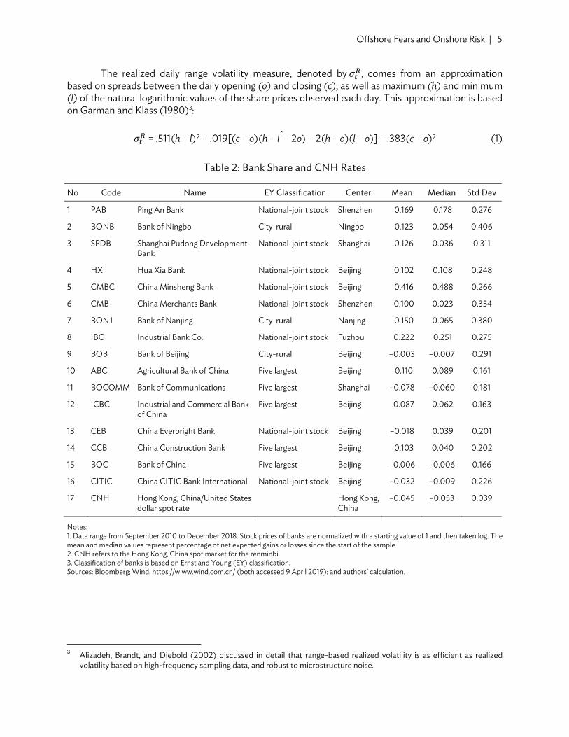
Table 2 lists the banks in our study. We follow the Ernst and Young classification, designating banks in three categories: the five largest state-owned banks, the national-joint-stock banks, and the city-rural banks. We normalize the share price indices with a starting value of unity for each bank, and then take the logarithmic values. Thus, the mean and median values represent percentage net expected gains or losses since the start of the sample. We see that all of the banks showed considerable volatility over the sample, between the starting date, September 2010, and the end date, December 2018.

Figure 1: Indices of Policy Uncertainty

Note: The straight line is the mean of all the 16 indices from September 2010 to December 2018. The broken line is the index of trade policy uncertainty, and the dotted one is the VIX, which is the implied volatility from options on the Standard and Poor’s 500 stock index. Sources: Baker, Bloom, and Davis (2016); Economic Policy Uncertainty. http://www.policyuncertainty.com/; Bloomberg; accessed on 9 April 2019); and authors’ calculation.

2011 2012 2013 2014 2015 2016 2017 20180

0.1

0.2

0.3

0.4

0.5

0.6

0.7

0.8

0.9

1.0

Mean index Trade uncertainty VIX


The realized daily range volatility measure, denoted by 𝜎 , comes from an approximation based on spreads between the daily opening (o) and closing (c), as well as maximum (h) and minimum (l) of the natural logarithmic values of the share prices observed each day. This approximation is based on Garman and Klass (1980)3:

𝜎 = .511(h – l)2 – .019[(c – o)(h – lˆ– 2o) – 2(h – o)(l – o)] – .383(c – o)2 (1)

Table 2: Bank Share and CNH Rates

No Code Name EY Classification Center Mean Median Std Dev

1 PAB Ping An Bank National-joint stock Shenzhen 0.169 0.178 0.276

2 BONB Bank of Ningbo City-rural Ningbo 0.123 0.054 0.406

3 SPDB Shanghai Pudong Development Bank

National-joint stock Shanghai 0.126 0.036 0.311

4 HX Hua Xia Bank National-joint stock Beijing 0.102 0.108 0.248

5 CMBC China Minsheng Bank National-joint stock Beijing 0.416 0.488 0.266

6 CMB China Merchants Bank National-joint stock Shenzhen 0.100 0.023 0.354

7 BONJ Bank of Nanjing City-rural Nanjing 0.150 0.065 0.380

8 IBC Industrial Bank Co. National-joint stock Fuzhou 0.222 0.251 0.275

9 BOB Bank of Beijing City-rural Beijing –0.003 –0.007 0.291

10 ABC Agricultural Bank of China Five largest Beijing 0.110 0.089 0.161

11 BOCOMM Bank of Communications Five largest Shanghai –0.078 –0.060 0.181

12 ICBC Industrial and Commercial Bank of China

Five largest Beijing 0.087 0.062 0.163

13 CEB China Everbright Bank National-joint stock Beijing –0.018 0.039 0.201

14 CCB China Construction Bank Five largest Beijing 0.103 0.040 0.202

15 BOC Bank of China Five largest Beijing –0.006 –0.006 0.166

16 CITIC China CITIC Bank International National-joint stock Beijing –0.032 –0.009 0.226

17 CNH Hong Kong, China/United States dollar spot rate

Hong Kong, China

–0.045 –0.053 0.039

Notes: 1. Data range from September 2010 to December 2018. Stock prices of banks are normalized with a starting value of 1 and then taken log. The mean and median values represent percentage of net expected gains or losses since the start of the sample. 2. CNH refers to the Hong Kong, China spot market for the renminbi. 3. Classification of banks is based on Ernst and Young (EY) classification. Sources: Bloomberg; Wind. https://wiww.wind.com.cn/ (both accessed 9 April 2019); and authors’ calculation.

3 Alizadeh, Brandt, and Diebold (2002) discussed in detail that range-based realized volatility is as efficient as realized

volatility based on high-frequency sampling data, and robust to microstructure noise.


As Yilmaz (2018) notes, volatilities tend to have right skewness so one can approximate normality by taking the logarithms of the range volatilities.

Figure 2 gives the median values of the realized volatility measures of these 16 onshore banks and the realized volatility of the offshore CNH market. We see that at the time of the European debt crisis at the beginning of the sample, there were closely related patterns of volatility. However, in the middle and end of the sample we see that the CNH market was more volatile than the onshore banks.

Given that the five largest banks have greater restrictions, due to Basel capital asset requirements, in Figure 3 we compare the median values of these banks with the banks either publicly owned or owned by municipal governments. They do not exhibit marked differences over the sample period.

Figure 2: Banking and Offshore CNH Range Volatilities

CNH = offshore Hong Kong, China spot market for the renminbi. Source: Authors’ calculation

2011 2012 2013 2014 2015 2016 2017 2018 2019

0

5

10

10–3 Mean and median bank volatility

2011 2012 2013 2014 2015 2016 2017 2018 20190

0.05

0.10

0.15

0.20

Offshore CNH volatility


Figure 3: Median Range Volatilities, Big Five, and Public City-Rural Banks

Notes: The big five banks are: Industrial and Commercial Bank of China, Bank of China, China Construction Bank, Agricultural Bank of China, and Bank of Communications. The public city-rural banks include the eight national-joint stock banks and the three city-rural banks. The eight national-joint stock banks are: Ping An Bank, Shanghai Pudong Development Bank, Hua Xia Bank, China Minsheng Bank, China Merchants Bank, Industrial Bank Co., China Everbright Bank, and China CITIC Bank International. The three city-rural banks are: Bank of Beijing, Bank of Nanjing, and Bank of Ningbo. Source: Authors’ calculation.

B. Regularization of the Big VAR-X Model

As seen above, there are no appreciable differences in the median volatility measures between the five largest banks and the other banks in the sample. For this reason, we explore the connectedness or contagion patterns within and across the banking classes and with the CNH markets. Following a series of papers by Diebold and Yilmaz (2012, 2013) and Yilmaz (2018), we measure connectedness by making use of forecast error variance decomposition matrices from vector autoregression with exogenous variable (VAR-X) estimation. Since we make use of daily data, we use a lag length of 5 days and a forecast error horizon of 20 days.

We apply the VAR model for the full sample but also make use of a rolling window of regressions of sample size 150 to estimate time-varying measures of connectedness. In addition to the 85 parameters for each variable in the VAR, representing the own-lag effects and the cross-lag effects for 15 variables with lag length 5, we specify a constant term and a set of 15 control variables, representing the EPU indices in Table 1.

2011 2012 2013 2014 2015 2016 2017 2018 2019

0

2

4

6

8

10

10–3 Big five

2011 2012 2013 2014 2015 2016 2017 2018 2019

0

5

10

10–3 Public city-rural


Given that the VAR-X model is a big VAR-X one, there is the need for regularization. We make use of the elastic net (EN) estimator due to Zou and Hastie (2005) for parameter reduction or regularization:

(2)

where 𝛽 denotes the elastic net estimator, which is a vector if 𝑖 > 1, 𝑦 is the observed daily range volatility calculated by equation (1) for the 16 banks and the CNH market,4 𝛽 is the parameter associated with 𝑥 in the VAR system, where 𝑥 is the explanatory variable entering the right hand side of the equations in the VAR system, which incorporates a lag length of 5 days of the daily ranged volatility for all banks and the CNH market (17 multiplied by 5 equals 85), plus a constant term and a set of 15 control variables in Table 1. This setup leads to 𝑘 = 101 for each equation in the VAR system. is the tuning parameter associated with the elastic net penalty term ∑ [(𝛼|𝛽 | ) + (1 − 𝛼) 𝛽 ], which is assumed to be positive. 𝛼 is the weight parameter that produces a convex combination of the least absolute shrinkage selection operator (lasso) and ridge penalty, and is assumed positive but less than 1. To be more specific, |𝛽 | is the lasso penalty, while 𝛽 is the ridge penalty.

As Yilmaz (2018) notes, the EN combines the lasso and ridge penalties through the tuning parameters {α, λ}. With α = 1, λ > 0, it is a lasso; it is a ridge estimator with α = 0, λ > 0. With λ = 0, of course, there is no penalty for large numbers of parameters, and the estimates are least squares.

The ordinary least squares estimator, with no penalty for large numbers of parameters, would allow for large numbers of small, insignificant cross effects and thus overstate degrees of connectedness among the dependent variables in the VAR-X model. By making use of the EN, we are minimizing the degree of interconnectedness among the variables, by eliminating variables which have small absolute or squared values. Thus, when we do find interconnectedness, the measure is a conservative estimate of the true connectedness.

Much like other, more familiar criteria for reducing parameters by altering lag length—such as Akaike, Schwartz, and Hannan-Quinn information criteria—the EN penalizes models for having too many parameters. With this net, the choice of the regularization parameters α, λ is the fundamental part. The two parameters control the strength of shrinkage and variable section. As such, well-selected parameters can improve both model prediction and interpretation, and is essential to the performance. However, excessively strong regularization may force important variables being left out of the model, which could harm both predictive capacity and the inferences drawn about the system being studied.

We set the parameter α = 0.5, and estimate the coefficients of the model for alternative values of λ. As λ increases, more and more parameters move to zero. One way to choose this parameter is to use a method based on cross validation. In this approach, we select a grid of values for λ, between λ = 0, and λ∗, the minimum λ which sets all of the coefficients 𝛽 = 0. We then select a set of out-of-sample mean squared error measures, based on holding out 20% of the sample for each specified λ over the grid. We thus select the optimal λ as the one which minimizes the average out-of-sample

4 Since we estimate the VAR system one equation at a time, here 𝑦𝑡 is scalar, representing the daily range volatility of one

bank or the CNH market at time t.

Enet

Min

t i iti

i ii

k

t

T

y x

22

111


mean squared error, based on five sets of holdouts of 20% of the data. We do this both for the full data set as well as for the smaller samples based on the rolling-window estimations.

We note that the coefficients 𝛽 are based on the full in-sample elastic net estimation with the prespecified tuning parameter, α, and the final optimal value of λ, coming from the cross-validation method. We estimate the coefficients in four steps:

1. specify α = 0.5 for the elastic net estimation, as a fixed hyperparameter; 2. full sample elastic net estimation with various λ; 3. cross validation with various λ; 4. choose the optimal result based on the average mean-squared out-of-sample errors.

C. Variance Decomposition and Systemic Risk

It is well known, of course, that the impulse response paths and forecast error-variance decomposition measures are sensitive to the ordering of the variables in the VAR model. Following the approach of Diebold and Yilmaz (2012), we make use of the generalized method for obtaining forecast error variance decomposition, due to Pesaran and Shin (1998), which does not rely on the Cholesky decomposition for orthogonal shocks.

This decomposition matrix is an asymmetric matrix and serves as a measure of both the inward and outward connectedness of each variable in the model. In particular, off-diagonal measures tell us how much of the innovations in each variable can be accounted for by the innovations in the other variables (inward connectedness) as well as how much each variable contributed to the overall forecast error of the other variables (outward connectedness).

Diebold and Yilmaz (2014) point out that this connectedness approach closely relates to measures of systemic risk. The inward-connectedness measure, they note, represents the exposures of individual banks to systematic shocks from the network as a whole, while the outward connectedness indicates the contribution of the individual bank to systemic network events (see Acharya et al. 2010 and Adrian and Brunnermeier 2016).

Of course, we expect these measures of systemic risk to change through time, over the course of the sample, as changes take place in banking regulations and as financial markets become more open. For this reason, we report these measures of systemic risk, not only for the full sample, but also as time-varying measures based on rolling-window regressions.

III. CONNECTEDNESS

As noted above, we wish to examine the connectedness between the risk measures in the CNH market and the volatility of the banking system. We first examine the interactions between the CNH market and all of the PRC banks. Then we look at the interactions between the CNH markets with the big five and with the national-joint-stock and city-rural banks. Finally, we examine the time-varying connectedness measures between the big five and the national-joint-stock and city-rural banks with the CNH markets.


A. Full Sample Connectedness

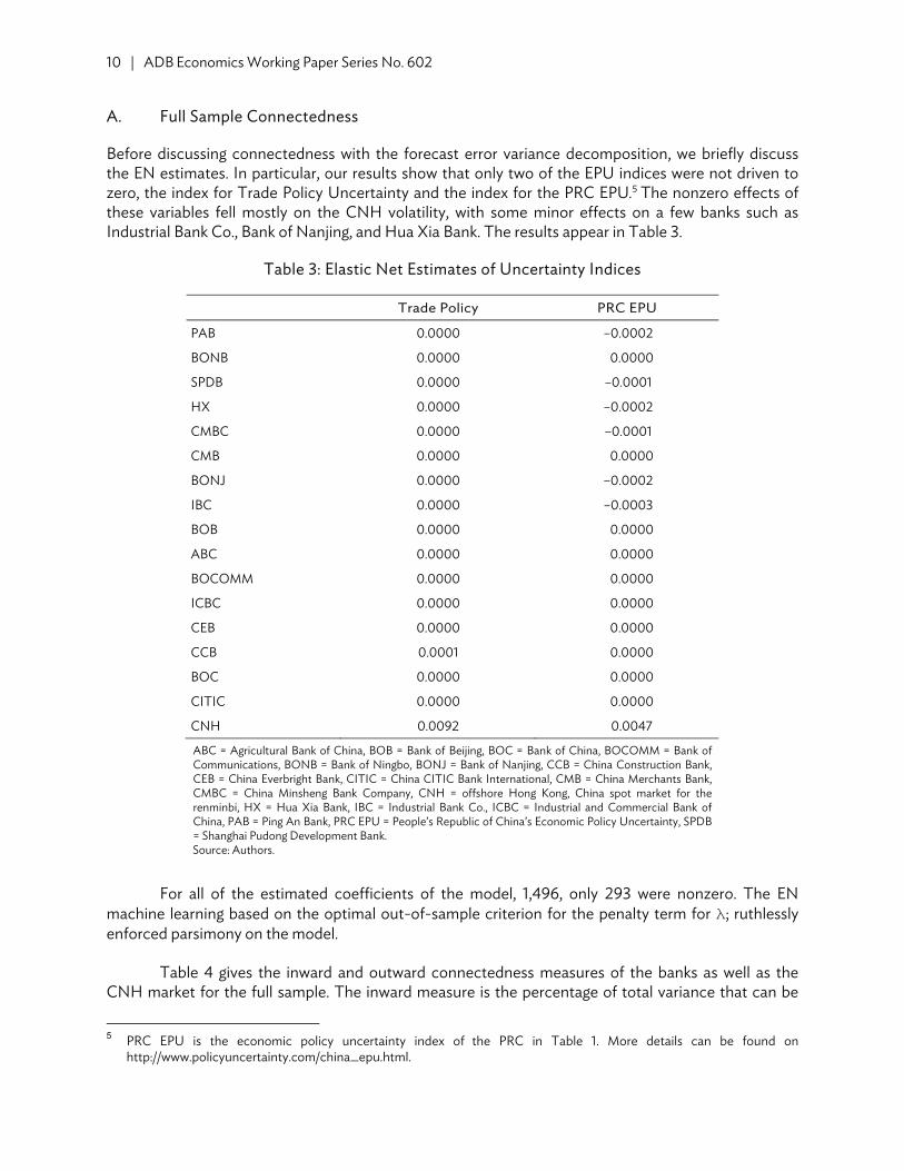
Before discussing connectedness with the forecast error variance decomposition, we briefly discuss the EN estimates. In particular, our results show that only two of the EPU indices were not driven to zero, the index for Trade Policy Uncertainty and the index for the PRC EPU.5 The nonzero effects of these variables fell mostly on the CNH volatility, with some minor effects on a few banks such as Industrial Bank Co., Bank of Nanjing, and Hua Xia Bank. The results appear in Table 3.

Table 3: Elastic Net Estimates of Uncertainty Indices

Trade Policy PRC EPU

PAB 0.0000 –0.0002

BONB 0.0000 0.0000

SPDB 0.0000 –0.0001

HX 0.0000 –0.0002

CMBC 0.0000 –0.0001

CMB 0.0000 0.0000

BONJ 0.0000 –0.0002

IBC 0.0000 –0.0003

BOB 0.0000 0.0000

ABC 0.0000 0.0000

BOCOMM 0.0000 0.0000

ICBC 0.0000 0.0000

CEB 0.0000 0.0000

CCB 0.0001 0.0000

BOC 0.0000 0.0000

CITIC 0.0000 0.0000

CNH 0.0092 0.0047

ABC = Agricultural Bank of China, BOB = Bank of Beijing, BOC = Bank of China, BOCOMM = Bank of Communications, BONB = Bank of Ningbo, BONJ = Bank of Nanjing, CCB = China Construction Bank, CEB = China Everbright Bank, CITIC = China CITIC Bank International, CMB = China Merchants Bank, CMBC = China Minsheng Bank Company, CNH = offshore Hong Kong, China spot market for the renminbi, HX = Hua Xia Bank, IBC = Industrial Bank Co., ICBC = Industrial and Commercial Bank of China, PAB = Ping An Bank, PRC EPU = People’s Republic of China’s Economic Policy Uncertainty, SPDB = Shanghai Pudong Development Bank. Source: Authors.

For all of the estimated coefficients of the model, 1,496, only 293 were nonzero. The EN machine learning based on the optimal out-of-sample criterion for the penalty term for λ; ruthlessly enforced parsimony on the model.

Table 4 gives the inward and outward connectedness measures of the banks as well as the CNH market for the full sample. The inward measure is the percentage of total variance that can be

5 PRC EPU is the economic policy uncertainty index of the PRC in Table 1. More details can be found on

http://www.policyuncertainty.com/china_epu.html.


explained by shocks from the other banks and the CNH market. By definition, the maximum value of the inward measure is 1. We see that for some banks, such as Hua Xia Bank, Bank of Beijing, China Merchants Bank, China Construction Bank, and Bank of China, a considerable proportion, more than 90%, of their volatility is due to systemic risks from other banks. For outward volatility, this is the amount of variation of the other banks' total volatility which is due to the specific bank in question. We see that only three banks, PAB, BONB, and ABC, are net transmitters of risk to the rest of the system. We also see that the CNH market is also a net transmitter of risk, but to a far lower degree than the PAB and BONB banks.

Table 4: Inward, Outward, and Net Connectedness

Inward Outward Net

PAB 0.291 7.137 6.846 BONB 0.667 2.885 2.218 SPDB 0.845 0.360 -0.485 HX 0.949 0.368 –0.581 CMBC 0.857 0.340 –0.517 CMB 0.915 0.167 –0.748 BONJ 0.863 0.402 –0.461 IBC 0.989 0.034 –0.955 BOB 0.956 0.083 –0.874 ABC 0.753 0.854 0.102 BOCOMM 0.951 0.311 –0.639 ICBC 0.644 0.083 –0.562 CEB 0.933 0.129 –0.804 CCB 0.974 0.097 –0.877 BOC 0.923 0.063 –0.860 CITIC 0.896 0.028 –0.868 CNH 0.025 0.091 0.066

ABC = Agricultural Bank of China, BOB = Bank of Beijing, BOC = Bank of China, BOCOMM = Bank of Communications, BONB = Bank of Ningbo, BONJ = Bank of Nanjing, CCB = China Construction Bank, CEB = China Everbright Bank, CITIC = China CITIC Bank International, CMB = China Merchants Bank, CMBC = China Minsheng Bank Company, CNH = offshore Hong Kong, China spot market for the renminbi, HX = Hua Xia Bank, IBC = Industrial Bank Co., ICBC = Industrial and Commercial Bank of China, PAB = Ping An Bank, SPDB = Shanghai Pudong Development Bank. Source: Authors.

Table 5 gives the measures of connectedness between the CNH market and the total banking system as well as to the three categories of banks.

What stands out in Table 5 is that the national-joint-stock banks have a much greater degree of connectedness with the CNH markets than the big five, but the direction of risk contagion is from the national-joint-stock banks to the CNH markets. For the full sample, the CNH market has a stronger effect on the national-joint-stock banks than on the big five and practically no effect on the city-rural banks.


Table 5: Full Sample Measures of Connectedness

CNH to Banks Banks to CNH

All 0.025 0.090

Big five 0.009 0.013

National-joint-stock 0.013 0.045

City-rural 0.000 0.014

CNH = offshore Hong Kong, China spot market for the renminbi. Notes: The big five banks are: Industrial and Commercial Bank of China, Bank of China, China Construction Bank, Agricultural Bank of China, and Bank of Communications. The public city-rural banks include the eight national-joint stock banks and the three city-rural banks. The eight national-joint stock banks are: Ping An Bank, Shanghai Pudong Development Bank, Hua Xia Bank, China Minsheng Bank, China Merchants Bank, Industrial Bank Co., China Everbright Bank, China CITIC Bank International. The three city-rural banks are: Bank of Beijing, Bank of Nanjing, and Bank of Ningbo. Source: Authors.

B. Time-Varying Connectedness

1. CNH Market Pressure on the Banking System as a Whole

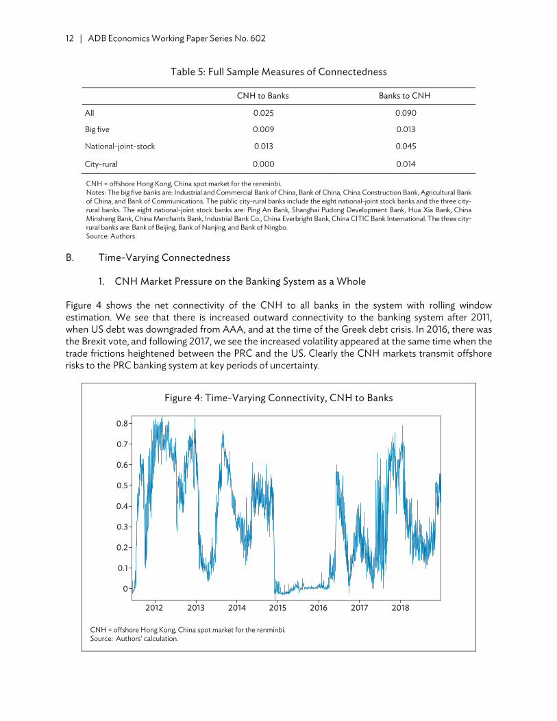
Figure 4 shows the net connectivity of the CNH to all banks in the system with rolling window estimation. We see that there is increased outward connectivity to the banking system after 2011, when US debt was downgraded from AAA, and at the time of the Greek debt crisis. In 2016, there was the Brexit vote, and following 2017, we see the increased volatility appeared at the same time when the trade frictions heightened between the PRC and the US. Clearly the CNH markets transmit offshore risks to the PRC banking system at key periods of uncertainty.

Figure 4: Time-Varying Connectivity, CNH to Banks

CNH = offshore Hong Kong, China spot market for the renminbi. Source: Authors’ calculation.

2012 2013 2014 2015 2016 2017 2018

0

0.1

0.2

0.3

0.4

0.5

0.6

0.7

0.8


2. CNH Market Pressure on the Big Five, National, and City-Rural Banks

Figure 5 illustrates the net outward connectedness between the CNH market volatility and the total volatility of the big five, national-joint-stock, and city-rural banks. We see little difference in the time pattern of the connectedness measures. All three are relatively large at the start of the sample and at the end of the sample. The only difference we note is that the national and city-rural bank volatility measures respond slightly before the big five banks in 2016.

Figure 5: Time-Varying Connectivity, CNH to Classes of Banks


3. Bank Pressure on the CNH Market

Figure 6 demonstrates the pressures from all of the banks to the CNH market. We see that it peaks in 2014, following a credit crunch in 2013. However, there is a large drop in the influence of the onshore banks in 2015. Funke et al. (2015) note that after August 2015, the People's Bank of China used the deviation of the offshore rate from the onshore central parity and a US dollar index as the key variables for determining the central parity. In short, the offshore exchange rate became an active policy anchor for setting the official PRC’s yuan (CNY) exchange rate.

Big five

2012

0.80.60.40.2

02013 2014 2015 2016 2017 2018

National-joint-stock

2012

0.80.60.40.2

02013 2014 2015 2016 2017 2018

City-rural

2012

0.80.60.40.2

0

2013 2014 2015 2016 2017 2018


Figure 6: Time-Varying Connectivity, All Banks to CNH Markets


Figure 7: Time-Varying Connectivity, Classes of Banks to CNH


2012 2013 2014 2015 2016 2017 2018

0.1

0.2

0.3

0.4

0.5

0.6

0.7

0.8

0.9

2012 2013 2014 2015 2016 2017 2018

0.050.100.15

0.20Big five

2012 2013 2014 2015 2016 2017 2018

0.20

0.40

0.60National-joint-stock

2012 2013 2014 2015 2016 2017 2018

0.10

0.20

0.30

City-rural


Figure 7 indicates the pressures from the three classes of banks on the CNH market. This figure shows that the national-joint-stock banks have a greater effect on the CNH market than the big five or the city-rural banks. We see a drop in their connectedness to the CNH markets after 2015. We also see, toward the end of the sample, as the Trade Index becomes more important, the effects of onshore banks, of any type, become less important for the CNH market volatility.

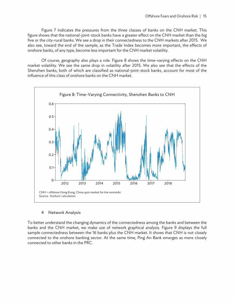
Of course, geography also plays a role. Figure 8 shows the time-varying effects on the CNH market volatility. We see the same drop in volatility after 2015. We also see that the effects of the Shenzhen banks, both of which are classified as national-joint-stock banks, account for most of the influence of this class of onshore banks on the CNH market.

Figure 8: Time-Varying Connectivity, Shenzhen Banks to CNH


4 Network Analysis

To better understand the changing dynamics of the connectedness among the banks and between the banks and the CNH market, we make use of network graphical analysis. Figure 9 displays the full sample connectedness between the 16 banks plus the CNH market. It shows that CNH is not closely connected to the onshore banking sector. At the same time, Ping An Bank emerges as more closely connected to other banks in the PRC.

2012 2013 2014 2015 2016 2017 20180

0.1

0.2

0.3

0.4

0.5

0.6


Figure 9 illustrates the net connectivity of the CNH to all banks in the system with a rolling window estimation. We see that there is increased outward connectivity to the banking system after 2011, when US debt was downgraded from AAA, and at the time of the Greek debt crisis. In 2016, the Brexit vote occurred, and, following 2017, we see increased volatility appeared at the same time as the trade frictions rose between the PRC and the US. Clearly, CNH markets transmit onshore risks to the PRC banking system at key periods of uncertainty.

Figure 9: Network Connectedness, Full Estimation

ABC = Agricultural Bank of China, BOB = Bank of Beijing, BOC = Bank of China, BOCOMM = Bank of Communications, BONB = Bank of Ningbo, BONJ = Bank of Nanjing, CCB = China Construction Bank, CEB = China Everbright Bank, CITIC = China CITIC Bank International, CMB = China Merchants Bank, CMBC = China Minsheng Bank, HX = Hua Xia Bank, IBC = Industrial Bank Co., ICBC = Industrial and Commercial Bank of China, PAB = Ping An Bank, SPDB = Shanghai Pudong Development Bank. Source: Authors.

CMBC

BOB

BOCHXIBC

CNH

SPDB

CITIC BONB

PAB

ABCCEB

ICBC

CMBCCB

BONJ

BOCOMM


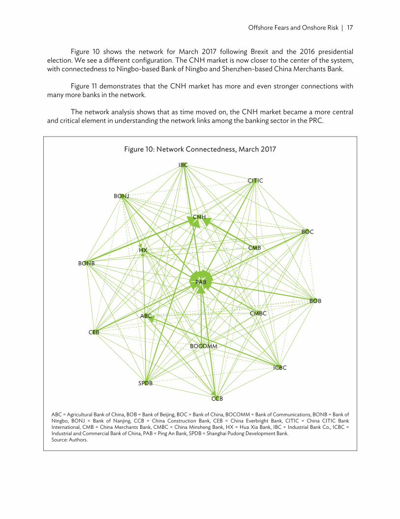
Figure 10 shows the network for March 2017 following Brexit and the 2016 presidential election. We see a different configuration. The CNH market is now closer to the center of the system, with connectedness to Ningbo-based Bank of Ningbo and Shenzhen-based China Merchants Bank.

Figure 11 demonstrates that the CNH market has more and even stronger connections with many more banks in the network.

The network analysis shows that as time moved on, the CNH market became a more central and critical element in understanding the network links among the banking sector in the PRC.

Figure 10: Network Connectedness, March 2017


CMBC

BOB

BOC

HX

IBC

CNH

SPDB

CITIC

BONB

PAB

ABC

CEB

ICBC

CMB

CCB

BONJ

BOCOMM


Figure 11: Network Connectedness, December 2018


IV. ROBUSTNESS: CNH VOLATILITY OR CNH–CNY SPREAD?

Funke et al. (2015) draw attention to the importance of the differential between the offshore CNH and the onshore CNY markets for PRC financial markets. What matters more, the volatility of the offshore market or the differential between the offshore and onshore markets?

Figure 12 illustrates the CNH range volatility and the absolute value of the spread between the offshore CNH and the onshore CNY market. This figure shows little difference. The peak periods of volatility correspond closely to the peak periods of the spread.

CMBC

BOB

BOC

HX

IBC

CNH

SPDB

CITIC

BONB

PAB

ABC

CEB

ICBC

CMB

CCB

BONJ

BOCOMM


Figure 12: CNH Volatility and Offshore and Onshore Spread

CNH = offshore Hong Kong, China spot market for the renminbi. Source: Authors.

A. Full Period Estimation with CNH–CNY Spread

For the overall sample, we find that the EPU index for financial liberalization is the most important control variable, rather than the EPU indices for trade policy or the PRC. As in the case of the volatility measure, this control variable only affects the spread variable.

Table 6 gives the inward, outward, and net connectedness measures for full sample estimation when we use the CNH–CNY spread rather the range volatility. We see little or no difference between Table 6 and Table 4. The banks having the strongest net outward connectedness measures remain Ping An Bank and Bank of Ningbo. The influence of the spread between the offshore and onshore markets appears to be smaller in absolute value, and now negative, relative to the influence of the range volatility of the offshore market.

2011 2012 2013 2014 2015 2016 2017 20180

0.05

0.10

0.15

0.20

CNH Vol

2011 2012 2013 2014 2015 2016 2017 20180

0.05

0.10

0.15

Spread


Table 6: Connectedness under Full Sample with CNH–CNY Spread

Inward Outward Net

PAB 0.304 7.159 6.855

BONB 0.664 2.886 2.222

SPDB 0.839 0.419 –0.420

HX 0.942 0.420 –0.521

CMBC 0.861 0.340 –0.521

CMB 0.914 0.159 –0.755

BONJ 0.864 0.412 –0.452

IBC 0.981 0.040 –0.942

BOB 0.957 0.076 –0.881

ABC 0.752 0.830 0.077

BOCOMM 0.955 0.286 –0.669

ICBC 0.664 0.101 –0.563

CEB 0.938 0.128 –0.810

CCB 0.971 0.100 –0.871

BOC 0.928 0.062 –0.866

CITIC 0.898 0.027 –0.871

CNH 0.028 0.014 –0.014

ABC = Agricultural Bank of China, BOB = Bank of Beijing, BOC = Bank of China, BOCOMM = Bank of Communications, BONB = Bank of Ningbo, BONJ = Bank of Nanjing, CCB = China Construction Bank, CEB = China Everbright Bank, CITIC = China CITIC Bank, CMB = China Merchants Bank, CMBC = China Minsheng Bank Company, CNH = offshore Hong Kong, China spot market for the renminbi, CNY = onshore spot market for the yuan, HX = Hua Xia Bank, IBC = Industrial Bank Co., ICBC = Industrial and Commercial Bank of China, PAB = Ping An Bank, SPDB = Shanghai Pudong Development Bank.. Source: Authors’ calculation.

B. Time-Varying Connectedness with CNH–CNY Spread

Figure 13 shows the time-varying measure of outward connectedness from the CNH–CNY spreads to banks. We see very similar patterns to those in Figure 4. The importance of the spreads is largest at the beginning of the sample and at the end, both at the time of Brexit and at the time of the trade tensions between the US and the PRC.

The results of this robustness check indicate that little difference shows up if we use the volatility of the offshore market or the spread between the offshore and onshore markets as our measure of exchange rate pressure on PRC banks.


Figure 13: Time-Varying Connectivity: CNH to Banks, with CNH–CNY Spread

CNH = offshore Hong Kong, China spot market for the renminbi, CNY = onshore spot market for the yuan. Source: Authors.

V. CONCLUSION

The results of this paper show the way offshore fears—signaled by volatility in the CNH Hong Kong, China spot market for the RMB-US dollar or by spreads between the offshore and onshore RMB markets—have become increasingly important sources of risk contagion for PRC banks. The growing role of the CNH market has shown that it directly affects the risks of the large big five banks as well as the national-joint-stock and city-rural banks, and not only in nearby Shenzhen, but also throughout the country. The risk measures also change the pattern of contagion among domestic onshore banks. PRC banking sector risks are not as insulated from offshore fears reflected in currency market volatility as thought.

For policy, the key implication is that overall banking share price volatility is not as insulated from the rest of the world as one might imagine, in the presence of limited capital mobility. In this process of gradual financial opening, the development of the more flexible CNH markets represents a further step in the internationalization of the RMB. But is it flexible enough? Or do discrepancies between the onshore and offshore markets simply magnify uncertainty for the financial system as a whole. While Friedman (1953) extolls the benefits of flexible exchange rates, it was in the context of a unified exchange rate system, not a dual system with onshore and offshore markets. Our conjecture is that a more flexible RMB could function as an effective shock absorber for the financial system when the offshore and onshore markets are integrated.

2012 2013 2014 2015 2016 2017 2018

0.1

0.2

0.3

0.4

0.5

0.6

0.7

0.8

REFERENCES

Acharya, Viral, Lasse Petersen, Thomas Philippon, and Matthew Richardson. 2010. “Measuring Systemic Risk.” Technical report. New York University.

Adrian, Tobias, and Markus Brunnermeier. 2016. “CoVaR.” American Economic Review 106 (7): 1705–41.

Alizadeh, Sassan, Michael Brandt, and Francis Diebold. 2002. “Range-Based Estimation of Stochastic Volatility Models.” Journal of Finance 57 (3): 1047–91.

Baker, Scott, Nicholas Bloom, and Steven J. Davis. 2016. “Measuring Economic Policy Uncertainty.” Quarterly Journal of Economics 131 (4): 1593–636.

Baker, Scott, Nick Bloom, Steven J. Davis, and Sophie Wang. 2013. “Economic Policy Uncertainty in China.” Unpublished.

Chow, Gregory, and An-loh Lin. 1971. “Best Linear Unbiased Interpolation, Distribution, and

Extrapolation of Time Series by Related Series.” Review of Economics and Statistics 53 (4): 372–75.

Diebold, Francis, and Kamil Yilmaz. 2012. “Better to Give than to Receive: Predictive Directional Measurement of Volatility Spillovers.” International Journal of Forecasting 28 (1): 57–66.

————. 2013. “Measuring the Dynamics of Global Business Cycle Connectedness.” PIER Working Paper Archive. Penn Institute for Economic Research, Department of Economics, University of Pennsylvania.

————. 2014. “On the Network Topology of Variance Decompositions: Measuring the Connectedness of Financial Firms.” Journal of Econometrics 182 (1): 119–34.

Friedman, Milton. 1953. “The Case for Flexible Exchange Rates.” In Essays in Positive Economics, 157–203. Chicago: University of Chicago Press.

Funke, Michael, Chang Shu, Xiaoqiang Cheng, and Sercan Eraslan. 2015. “Assessing the CNH and CNY Pricing Differential: Role of Fundamentals, Contagion and Policy.” Journal of International Money and Finance 59 (C): 245–62.

Garman, Mark, and Michael Klass. 1980. “On the Estimation of Security Price Volatilities from Historical Data.” The Journal of Business 53 (1): 67–78.

Gu, Li, and Paul McNelis. 2013. “Yen/Dollar Volatility and Chinese Fear of Floating: Pressures from the NDF Market.” Pacific-Basin Finance Journal 22 (C): 37–49.

Park, Cyn-Young, and Kwanho Shin. 2018. “Global Banking Network and Regional Financial Contagion.” ADB Economics Working Paper Series No. 546.

Pesaran, H. Hashem, and Yongcheol Shin. 1998. “Generalized Impulse Response Analysis in Linear Multivariate Models.” Economics Letters 58 (1): 17–29.

24 | References

Reinhart, Carmen M., and Kenneth S. Rogoff. 2013. “Banking Crises: An Equal Opportunity Menace.” Journal of Banking and Finance 37 (11): 4557–73.

Yilmaz, Kamil. 2018. “Bank Volatility Connectedness in South East Asia.” KoçUniversity-TUSIAD Economic Research Forum Working Papers 1807.

Zou, Hui, and Trevor Hastie. 2005. “Regularization and Variable Selection via the Elastic Net.” Journal of the Royal Statistical Society: Series B (Statistical Methodology) 67 (2): 301–20.


ASIAN DEVELOPMENT BANK6 ADB Avenue, Mandaluyong City1550 Metro Manila, Philippineswww.adb.org

Offshore Fears and Onshore Risk Exchange Rate Pressures and Bank Volatility Contagion in the People’s Republic of China

This study examines whether the spot market in Hong Kong, China for offshore Chinese currency (CNH) acts as a shock absorber for the financial system of the People’s Republic of China (PRC). It finds that the CNH market may actually transmit the risks from offshore economic policy uncertainty to the PRC’s banking system. The analysis suggests that further offshore exchange market movements arising from news, such as increasing trade friction with the United States, would generate greater volatility in the Chinese banking sector.

About the Asian Development Bank

ADB is committed to achieving a prosperous, inclusive, resilient, and sustainable Asia and the Pacific, while sustaining its efforts to eradicate extreme poverty. Established in 1966, it is owned by 68 members —49 from the region. Its main instruments for helping its developing member countries are policy dialogue, loans, equity investments, guarantees, grants, and technical assistance.

OFFSHORE FEARS AND ONSHORE RISKEXCHANGE RATE PRESSURES AND BANK VOLATILITY CONTAGION IN THE PEOPLE’S REPUBLIC OF CHINA


ADB ECONOMICSWORKING PAPER SERIES

NO. 602

December 2019

Documents

About the Asian Development Bank OFFSHORE FEARS AND