ABSTRACT - atmos.umd.eduekalnay/dissertations/Grunmann... · ABSTRACT Title: VARIATIONAL DATA ASSIMILATION OF SOIL MOISTURE INFORMATION ... Dusanka Zupanski and Prof. Ferdinand Baer

ABSTRACT

Title: VARIATIONAL DATA ASSIMILATION OF

SOIL MOISTURE INFORMATION

Pablo J. Grunmann, Doctor of Philosophy, 2005

Directed By: Professor Eugenia Kalnay, Department of

Meteorology

Doctor Kenneth Mitchell, National Centers for

Environmental Prediction

This research examines the feasibility of using observations of land surface

temperatures (in principle available from satellite observations) to initialize soil

moisture (which is not available on a continental scale). This problem is important

because it is known that wrong soil moisture initial conditions can negatively affect

the skill of numerical weather prediction models.

Since this problem requires the availability of a good soil model, considerable

effort was devoted to the improvement of several aspects of the NCEP Noah land

surface model and its numerical properties (reliability, efficiency, updates and

differentiability). When tested against the experimental station data at Champaign, IL

collected by Dr. Tilden Meyers of NOAA/ARL, where the surface fluxes,

precipitation, and surface temperature were available, the Noah model forced with

observed downward radiative surface fluxes and near-surface meteorology, including

precipitation, was able to reproduce the observations quite well.

A method for data assimilation was developed and tested, in a manner similar

to 4-dimensional variational assimilation (4D-Var) in the sense of applying the

temporal behavior of the observed variable but with a single spatial dimension (land

surface models are typically “column models”, as they do not usually compute

horizontal derivatives). The results show that it is indeed possible to assimilate land

surface temperature and use it to correct soil moisture initial conditions, which may

manifest significant errors if, for example, the precipitation forcing the model is

significantly biased. This is true, however, only if the surface forcings besides

precipitation are essentially correct. When surface forcing come from the North

American Land Data Assimilation System (NLDAS) as they would be available for

operational use over the US, the results are not satisfactory. This is because the

assimilation changes the soil moisture to correct for problems in the simulated land

surface temperature that are at least partially due to other sources of errors, such as

the surface radiative fluxes. We suggest that in order to succeed in the soil moisture

initialization, more (and more accurate) observations are needed in order to constrain

the dependence of the observation part of the cost function solely on soil moisture.

VARIATIONAL DATA ASSIMILATION OF SOIL MOISTURE INFORMATION

By

Pablo J. Grunmann

Dissertation submitted to the Faculty of the Graduate School of theUniversity of Maryland, College Park, in partial fulfillment

of the requirements for the degree ofDoctor of Philosophy

2005

Advisory Committee:Prof. Eugenia Kalnay, ChairDr. Kenneth MitchellProf. Dalin ZhangProf. Ferdinand BaerProf. James CartonProf. Ruth DeFries

ii

Acknowledgements

I am very grateful to Dr. Kenneth Mitchell and Prof. Eugenia Kalnay, for their

unlimited support, inestimable help and suggestions. I would like to thank Dr.

Dusanka Zupanski and Prof. Ferdinand Baer for their help during my academic

journey and research phase of the work. I am grateful to all friends and colleagues of

the Environmental Modeling Center (EMC) of the National Centers for

Environmental Prediction (NCEP) and the faculty of the Department of Meteorology

of the University of Maryland for being always there when I needed them.

I have a debt of gratitude to CAPES (Coordenação de Aperfeiçoamento do

Pessoal de Nível Superior) and NCEP/EMC for their financial support.

All my family was very supportive and helped in numerous ways throughout

these years.

iii

Table of Contents

ABSTRACT............................................................................................................................... i

Acknowledgements................................................................................................................... ii

Table of Contents..................................................................................................................... iii

List of Tables ........................................................................................................................... vi

List of Figures ......................................................................................................................... vii

Chapter 1 Introduction........................................................................................................... 14

1.1 Specific goals of this dissertation ......................................................................... 17

Chapter 2 Theoretical overview ............................................................................................ 19

2.1 General approach .................................................................................................. 19

2.1.1 The problem of model performance versus parameters and

initial conditions................................................................................ 20

2.2 Variational assimilation ........................................................................................ 21

2.2.1 Cost Function .................................................................................... 22

2.2.2 Cost Function Analysis ..................................................................... 24

2.2.3 Gradient and Minimum of the Cost Function ................................... 30

2.2.4 Tangent Linear Model and Adjoint................................................... 31

2.2.5 Deriving the data assimilation tools for the Noah LSM ................... 33

Chapter 3 Description of the Noah Land Surface Model (Noah LSM)................................. 35

3.1 Water component .................................................................................................. 36

3.1.1 Surface Water Budget ....................................................................... 36

3.1.2 Canopy Evaporation: ........................................................................ 38

3.2 Energy component ................................................................................................ 41

iv

3.2.1 Relationship between Soil Moisture Content and Land

Surface Temperature ......................................................................... 41

3.2.2 Surface Energy Balance .................................................................... 44

3.2.3 Soil heat flow .................................................................................... 44

3.3 Order of Computations ......................................................................................... 44

Chapter 4 Data Sources Utilized ........................................................................................... 47

4.1 Reference site flux station (Tilden Meyers site) ................................................... 47

4.1.1 Filling in gaps of missing data in land surface forcing ..................... 48

4.2 NLDAS forcing..................................................................................................... 49

4.3 GOES land surface temperature............................................................................ 50

Chapter 5 Evaluation and Improvement of the Noah Land Surface Model

Performance .......................................................................................................... 51

5.1 Improved physics .................................................................................................. 52

5.1.1 Soil drainage ..................................................................................... 54

5.1.2 Frozen soil state iteration .................................................................. 57

5.2 Improved differentiability..................................................................................... 62

5.2.1 Example of singular behavior with certain functions in the

tangent linear model, and proposed solution. ................................... 62

5.3 Vertical diffusion of soil water during freezing.................................................... 65

5.4 Sensitivity to initial conditions ............................................................................. 69

Chapter 6 Generation and validation of the model control run. ............................................ 75

6.1 Multi-year spin-up of initial land states ................................................................ 75

6.2 Validation against reference site flux station........................................................ 80

Chapter 7 Data Assimilation Experiments ............................................................................ 85

7.1 Assimilating ideal synthetic data: Identical Twin Experiments ........................... 89

v

7.1.1 Degradation of precipitation forcing................................................. 89

7.1.2 Assimilating the LST of the control run ........................................... 91

7.2 Assimilating real data ......................................................................................... 104

7.2.1 Assimilating LST from the reference site station ........................... 105

7.2.2 Surface forcing from the North American Land Data

Assimilation System (NLDAS) ...................................................... 110

7.2.3 Assimilating LST from the GOES satellite .................................... 120

7.3 Conclusions from the ideal and real data assimilation experiments. .................. 125

Chapter 8 Conclusions......................................................................................................... 127

Appendices............................................................................................................................ 129

Appendix A: Limitations to the convergence of a finite-difference approximation

scheme to the derivative in the presence of round-off errors. ................................................ 129

Bibliography ......................................................................................................................... 131

vi

List of Tables

Table 1 Exponential decay e-folding time versus the length of spin-up used for the

exponential curve fit and whether the initial conditions were on the moist or dry

extremes. ............................................................................................................. 80

Table 2: Schematic table of identical twin (perfect model) experiments. .................. 88

Table 3: Schematic table of non identical twin experiments. ..................................... 88

vii

List of Figures

Figure 2-1 Schematic of the setting for changes to the model’s parameters or initial

conditions based on its adherence to observations. ............................................ 20

Figure 2-2 Example of the cost function (all terms) and its background component

computed during a high sensitivity period over the entire range of the control

variable, which represents the possible change to the initial conditions. ........... 29

Figure 2-3 Same as Figure 2-2 but for a low sensitivity period.................................. 30

Figure 3-1 Soil moisture stress factor in the plant transpiration, Et (example). ........ 40

Figure 3-2 Illustration of the NCEP LSM heat budget at the surface (adapted from Ek

and Mahrt (1991)). .............................................................................................. 42

Figure 3-3 Illustration of the NCEP LSM moisture budget (adapted from Ek and

Mahrt (1991))...................................................................................................... 43

Figure 4-1 Example of filling the gaps in the necessary forcing with the use of

appropriately converted alternative data. ............................................................ 49

Figure 5-1 Ground heat flux (W/m2) for the model versus observations using the old

soil thermal conductivity formulation. ................................................................ 52

Figure 5-2 Sensible heat flux (W/m2) for the model versus observations using the old

soil thermal conductivity formulation................................................................. 53

Figure 5-3 Soil thermal conductivity as calculated by the new subroutine compared to

the old one (marked with circles) for three main types of soils (marked with

specific line-types). ............................................................................................. 54

Figure 5-4 Hydraulic conductivity K(θ) (logarithmic scale), for 3 soil types, as a

function of soil moisture content (volumetric). .................................................. 55

Figure 5-5 Hydraulic diffusivity D(θ) (logarithmic scale), for 3 soil types, as a

function of soil moisture content (volumetric). .................................................. 56

Figure 5-6 Drainage test with the old code, isolating the gravitational effects. ......... 56

viii

Figure 5-7 Drainage test with the corrected code. ...................................................... 57

Figure 5-8 Graphs of the left hand sides of (5.1) and (5.4) as functions of frozen soil

moisture content, F(θ ice ) and L(θ ice ), respectively. The vertical blue line (SMC)

indicates the total soil moisture content ( iceliqtotal θθθ += ), a line that θ ice cannot

cross. ................................................................................................................... 59

Figure 5-9 Collected events of the Newton solver calls during a regular 1-year

simulation with the model and the number of iterations required for the solution

organized by temperature given as input. ........................................................... 60

Figure 5-10 Event distribution (logarithmic scale) of all calls to the Newton solver

during a regular 1-year simulation with the model by the number of iterations

required for the solution...................................................................................... 61

Figure 5-11 Percentage distribution of all calls to the Newton solver during a regular

1-year simulation with the model by the number of iterations required for the

solution................................................................................................................ 62

Figure 5-12 Weights for transition from the unfrozen to the partially frozen hydraulic

diffusivity behavior as function of the presence of volumetric frozen soil water

content................................................................................................................. 67

Figure 5-13 Resulting hydraulic diffusivity at the transition from unfrozen to partially

frozen soil for the old (VK), step (D) and the new (Weighted) approaches. ...... 68

Figure 5-14 Magnification of the ordinates’ axis of Figure 5-13 showing the strong

adherence of the weighted approach to the magnitudes prescribed by the D

approach as soil moisture content freezes........................................................... 68

Figure 5-15 Magnification of the abscissas’ axis of Figure 5-13 showing the weighted

approach matching the old (VK) behavior in magnitude and first derivative

(slope) at the transition from unfrozen to partially frozen soil moisture content.

............................................................................................................................. 69

ix

Figure 5-16 Volumetric soil moisture content (SMC) output from five months

simulations using the model for two different initializations of soil moisture,

0.250 and 0.350 (volumetric). First layer. .......................................................... 70



0.250 and 0.350 (volumetric). Second layer. ...................................................... 71



0.250 and 0.350 (volumetric). Third layer. ......................................................... 72

Figure 5-19 Volumetric soil moisture content (SMC) output from a five months’

simulation of the model for two different initializations of soil moisture, 0.250

and 0.350 (volumetric). Fourth layer. ................................................................. 73

Figure 5-20 Impact of the initial soil moisture content for two different initializations

of soil moisture, 0.250 and 0.350 (volumetric). Latent heat flux, 1 week. ......... 74

Figure 6-1 Convergence to a common equilibrium after a few years of spin-up

cycling starting from the opposite extremes of soil moisture, dry and moist. .... 76

Figure 6-2 RMS of the spin-up from the dry extreme conditions with respect to

equilibrium and its exponential fit based on the first seven years of adjustment.

............................................................................................................................. 77


equilibrium and its exponential fit based on the first three years of adjustment. 78

Figure 6-4 RMS of the spin-up from the moist extreme conditions with respect to

equilibrium and its exponential fit based on the first three years of adjustment. 78


equilibrium and its exponential fit based on the first year of adjustment. .......... 79

Figure 6-6 Land surface temperature from the model 1998 control run versus

observations from the ground station and its corresponding least squares linear

fit. ........................................................................................................................ 80

x

Figure 6-7 Sensible heat flux from the model 1998 control run versus observations

from the ground station and its corresponding least squares linear fit. .............. 81

Figure 6-8 Latent heat flux from the model 1998 control run versus observations from

the ground station and its corresponding least squares linear fit. ....................... 82

Figure 6-9 Ground heat flux from the model 1998 control run versus observations

from the ground station and its corresponding least squares linear fit. .............. 83

Figure 6-10 Same as Figure 6-9 but with the season in which freezing occurs

removed............................................................................................................... 84

Figure 6-11 Same as Figure 6-9 but just for the season in which freezing occurs ..... 84

Figure 7-1 Experiment 1. Soil moisture content evolution for the control run (black

line) and data assimilation run (blue line). Third soil layer. ............................... 93

Figure 7-2 Experiment 1. Soil moisture profiles before (blue) and after (black) data

assimilation event 1 (mid-May) versus control (“truth” in red). Soil layer 1 is

from the surface to 10 cm deep, soil layer 2 is from 10 cm to 40 cm deep, soil

layer 3 is from 40 cm to 1 m deep and soil layer 4 is from 1 m to 2m deep. Plant

roots are present in layers 1 to 3. ........................................................................ 94

Figure 7-3 Experiment 1. Same as Figure 7-2, for data assimilation event 2 (July). . 95

Figure 7-4 Experiment 1. Same as Figure 7-2, for data assimilation event 3

(September)......................................................................................................... 95

Figure 7-5 Experiment 1. Same as Figure 7-2, for data assimilation event 4 (end of

October). ............................................................................................................. 96

Figure 7-6 Experiment 2. Soil moisture content evolution for the reference 2 run

(black line, considered as truth) and data assimilation run (blue line). Third soil

layer..................................................................................................................... 97

Figure 7-7 Experiment 2. Soil moisture profiles before and after data assimilation

event 1 (mid-May) versus reference. .................................................................. 98


(black line) and data assimilation run (blue line). Second soil layer. ................. 99

xi


event 1 (mid-May) versus reference (red). ....................................................... 100


event 2 (July) versus reference (red)................................................................. 100


event 3 (September) versus reference (red). ..................................................... 101


event 4 (end of October) versus reference (red). .............................................. 101


(black line) and data assimilation run (blue line). Second soil layer. ............... 103


event 1 (mid-May) versus reference (red). ....................................................... 104

Figure 7-15 Experiment 5. Using a cost function of 3 ½ days. Soil moisture content

evolution for the control run (black line) and data assimilation run (blue line).

Soil layer 3. ....................................................................................................... 107

Figure 7-16 Experiment 5. Using a cost function of 11 days 20 hrs. Soil moisture

content evolution for the control run (black line) and data assimilation run (blue

line). Soil layer 3............................................................................................... 108


event 1 (mid-May) versus control..................................................................... 109

Figure 7-18 Experiment 5. Land surface temperature (LST, K) as 1) observed by

ground station (dotted), 2) simulated by control run (red) and 3) simulated by run

assimilating the ground station (blue)............................................................... 110

Figure 7-19 Experiment 6. NLDAS forced run with assimilation of LST from the

reference site ground station. Soil layer 3 moisture content evolution............. 112


event 3 (September) versus control................................................................... 113

xii


event 4 (end of October) versus control............................................................ 114


control run. Soil moisture evolution for model soil layer 3. ............................. 117


event 1 (mid May) versus control. .................................................................... 118

Figure 7-24 Experiment 7. Land surface temperature (LST) diurnal cycles during the

time window of data assimilation event 1. Shown here are control (red) and

NLDAS forced run (blue dashed line). ............................................................. 119

Figure 7-25 Soil moisture effect on land surface temperature diurnal cycle by

comparison between model runs in which one of them (blue line) received less

precipitation. ..................................................................................................... 119

Figure 7-26 Solar radiation effect on land surface temperature (LST) diurnal cycle by

comparison between model runs in which one of them received less solar

radiation forcing (70%). The radiation reduced run (blue line) shows smaller

LST amplitude. ................................................................................................. 120

Figure 7-27 Experiment 8. Soil moisture content evolution for the control run (black),

the NLDAS forced GOES LST data assimilation run (blue) and the NLDAS

forced run without data assimilation (dotted red). Third soil layer. ................. 122


event 1 (early April) versus control. ................................................................. 123


event 2 (mid April) versus control. ................................................................... 123


event 3 (late April) versus control. ................................................................... 124


event 4 (early September) versus control.......................................................... 124

xiii


event 5 (mid September) versus control. .......................................................... 125

14

Chapter 1

Introduction

Land-surface and soil hydrology models used as a lower boundary condition

by coupling with general circulation, climate or weather forecast models have been

recognized, over the past few decades, as vital to the quality of the results.

Consequently, progressively more sophisticated land surface models have been

developed and incorporated for such uses.

In general, computational time constraints and the difficulty in establishing

initial conditions in the soil has been a barrier for the use of the most sophisticated

land surface models in operational settings. Fortunately, the recent advances in

computational power allowed the incorporation of more complex and accurate land-

surface models. Still, the problem of estimating initial conditions for soil variables,

given that observations of these variables are not generally available, remains an

important challenge.

Early studies on the role of soil water (Namias, 1958) within the climate

system brought attention to the need of considering surface fluxes and runoff, as

affected by the variability of soil moisture. This justified the development of soil

models - such as the so-called “bucket model” (Manabe, 1969) - to take into account

the evolution of soil moisture and interaction with evaporation and runoff. In 1978,

Deardorff showed the importance of the contribution of vegetation to the latent heat

flux (evapotranspiration).

At the present time, land-surface models coupled with atmospheric models are

expected to reproduce the evolution of land-surface-atmosphere fluxes and soil

variables with reasonable accuracy given proper initial conditions and forcing.

Water storage in the soil affects directly evapotranspiration, soil heat storage,

thermal conductivity, and the partitioning of energy between latent and sensible

fluxes. As a result, it influences the moisture and temperature in the planetary

boundary layer and, consequently, the evolution and amount of cloudiness and

precipitation (Pan and Mahrt, 1987, Garratt, 1993).

15

Given recent advances in the state-of-the-art of numerical weather prediction

models, the quality of the simulation of the land-surface processes is having a larger

impact on the models, due to the increased requirement of accurate lower boundary

conditions to interact with the atmospheric models (Chen, F. et al., 1997). For this

reason, the quality of the simulation of the soil moisture field is of great importance in

order to obtain a proper simulation of land-surface physics and, consequently,

positively affect the quality of the weather forecasts (Viterbo and Illari, 1994; Koster

and Suarez, 2003).

One problem that has not yet been overcome is how to adjust the soil moisture

initial fields (Betts et al., 1996). This problem has serious consequences because,

given that soil moisture is a slowly evolving variable, an error in the initial condition

will affect the quality of the simulation for a long period of time, even if the correct

precipitation is observed and specified (as seen in the experiments described in

sections 5.4 and 6.1).

Soil moisture content values are not observed regularly over large areas,

making the use of direct soil moisture observations in the data assimilation system

impossible. Instead it becomes necessary to use indirect observations of soil moisture,

something made possible by its relationship to other observed fields.

Another possible approach is the initialization of soil moisture from

climatology as opposed to deriving or inferring it with the use of current observations.

The past common approach in most operational numerical weather prediction (NWP)

models has been to initialize soil moisture for the forecast cycle with values obtained

either from a climatological database or by letting the soil moisture content, as a

prognostic variable, to be cycled on itself in continuous adjustment with the rest of

the model (Viterbo and Beljaars, 1995). The use of climatological values has the

disadvantage of not reflecting real conditions associated to recent past evolution and,

therefore, an inherent inability to adapt to anomalous conditions such as wet or dry

spells. On the other hand, cycling the soil moisture content as a prognostic variable

forced by model precipitation and surface fluxes without corrections derived from

observations, may lead to drifting which is seen as a departure from realistic soil

16

moisture over time. This can be produced by inaccuracies in the forcing provided by

the companion models, usually radiation and precipitation, both affected by the

quality of the prediction of cloudiness within the atmospheric model. As a result, on a

time scale of weeks to months, the prediction errors can grow through complex

feedback loops, causing excessive accumulation or depletion of soil water stored,

leading to systematic under- or overestimation of the actual land-surface evaporation

(Viterbo, 1996). At NCEP, the global model in operation, using a version of Noah

land surface model for the treatment of land surface and soil variables, applies

nudging towards climatology in the Global Data Assimilation System (GDAS) cycle

on a 60-day time scale as a means to curtail the effects of drifting (e.g., Kistler et al,

2001). In the ETA model, the soil moisture was being initialized with analysis from

the global model; but now, it is cycled continuously on itself (Mitchell, 1998, etc,

personal communication).

In this context, it seems desirable to develop data assimilation approaches that

could provide the necessary initial soil moisture values derived from non-soil

moisture observations, while being consistent with the weather forecast model and

sensitive to recent past evolution.

The strong influence of the soil moisture on surface fluxes that, in turn, affect

low-level atmospheric parameters, suggests that it is possible to infer a correction to

the soil moisture content values based on information from prediction errors on

sensitive variables at the lower levels of the atmospheric model (Mahfouf, 1991,

Bouttier, et al., 1993).

Another approach could be to infer the corrections to soil moisture from the

surface fluxes themselves (van den Hurk et al., 1997; Jones et al., 1998), thus

avoiding some of the disadvantages of using error information from near surface

parameters, namely, miscalculations caused by components of these errors that have

no relationship with soil moisture, such as effects from horizontal advection and

situations in which surface fluxes effects are small compared to other effects.

However, this method requires having information about the surface fluxes, which,

until recently, was not routinely available. As new surface observations became

17

available with the recent implementation of GEWEX GOES satellite surface products

retrieval (Gutman G, 1994; Pinker et al., 1996; Tarpley et al., 1996), there is a new

perspective on the range of observations relevant to soil moisture data assimilation

and their feasibility of implementation on future operational use.

1.1 Specific goals of this dissertation

The main goal of this thesis is to attempt to develop an approach that could

provide the necessary soil moisture values derived from available non-soil

observations while being consistent with the model physics and sensitive to recent

past evolution. For this purpose, the following steps are defined for this work:

I. Show that the land surface model is realistic at updating the state variables

and reproducing accurately the land-atmosphere fluxes when correct forcing

and reasonable initial conditions are given. This includes making the

necessary adjustments and improvements to the model as well as testing and

validating the land-surface model at target sites where surface atmospheric

fluxes and soil data are available. The new version of the NCEP model should

be able to produce a reasonably unbiased response when verified by

observations. Additionally, this upgraded model should also be made to be

differentiable as much as necessary to produce the tangent linear of this code.

Having this version ready, it will produce a control run (from nearly ideal

initial conditions and forcing). A second run with errors and biases in initial

conditions or forcing should show a cumulative degraded response due to,

e.g., precipitation bias, in contrast to that of the control run response.

II. Develop a data assimilation scheme based on variational techniques. These

techniques need to find the minimum of a cost function, procedure that may

require computing the gradient of such cost function with respect to the

control variables (e.g. initial time soil moisture correction). This gradient

would be better calculated by using a differential of the FORTRAN source

code (such as the linear tangent or the adjoint model). Consequently,

18

observations (other than soil moisture) can be used to adjust the trajectory of

key state variables to improve the response of the model.

III. Test and assess possible improvements in the predictive ability of the model

due to data assimilation by comparing the results with similar experiments but

without data assimilation.

19

Chapter 2

Theoretical overview

In this chapter we discuss the formulation of the data assimilation problem for

finding optimal initial conditions for the model’s initial soil moisture and optimal

parameters.

2.1 General approach

The ability to simulate dynamical-physical processes in nature through the use

of a computer model requires a reasonable reproduction in time of the behavior of the

variables representing those processes. This depends on the quality of representation

of the mechanisms involved and matching the states of the model variables with those

of the processes being simulated. In principle, if it were possible to find a perfect

match at the initial time between the processes states and the model’s (initial

condition), the increasing disagreement over time between the two would be

attributed mostly to the model’s limitation in including and performing accurately all

the required elements and their dynamics as involved in those processes.

In reality, neither condition is completely satisfied but it is desirable to

approximate them in a cost-effective way. In this work, we are mostly concerned with

finding initial conditions given that the model is satisfactorily capable at reproducing

the desired processes from there.

What is meant by a trajectory is the set of time series of the state and output

variables calculated by the model (forecast). If the time-span is long enough, a subset

composed of just a few critical variables is sufficient to represent the model’s

trajectory, this is explained by the model’s physical constraint between variables

(through the model equations). Given this, it is possible to rely on one or very few

observed variables (but over a time period) and still expect the model to change its

entire trajectory consistently towards matching more closely the behavior of this or

these variables.

20

2.1.1 The problem of model performance versus parameters and

initial conditions

Let’s call the whole set of model’s state variables plus time-dependent outputs

as the set of "model predictions" (model calculations). This is everything the model

produces by calculating forward in time given a set of initial conditions plus

parameters (given or pre-determined).

Figure 2-1 Schematic of the setting for changes to the model’s parameters or initial

conditions based on its adherence to observations.

The problem of improving model performance by making changes to the set

of "given" values (model initial conditions and/or model parameters) relies on being

able to compute model error, i.e., a measure of the discrepancy between the whole set

of "model predictions" and observations (Figure 2-1).

If enough observations were available as to verify each and every element of

the set of "model predictions", it would be possible to construct a model error

function that takes as input the multi-dimensional vector with the whole set of the

"given" and produces a scalar number. This should also take into account an

appropriate normalization for the contribution to the error by each and every one

element of the "model predictions" over a period of time (verification window) to the

total error.

21

Even in this scenario it is quite likely to find more than one set of the "given"

producing minima in the error function as a result of compensation or contradicting

effects within elements of the "given" set. In some cases, increasing the time-span of

the verification window would reduce the number of dissimilar sets that produce a

minimum in the error function (for example, two different sets of the "given" may

seem equally satisfactory over a certain month but one of them seems better when the

verification window extends over many months or the entire year). If many different

sets of possible "given" are still found after all attempts, a simplification of the model

may be considered, which could mean just to set some elements of the "given" as

constant (no longer part of the error function domain) but they have to be identified

and chosen. This deals into the limitations of models mandated by our limitations in

verification.

In real life, having enough observations as to verify each and every element of

the set of "model predictions" may certainly not be possible. Instead, only a subset of

"model predictions" can be verified. This increases the likelihood of having different

sets of "given" that appear to minimize the model error function.

2.2 Variational assimilation

The basic variational assimilation problem, for the purpose of correcting the

initial conditions to be used by the model, consists of: first, computing a function

(cost function) that measures the distance between the observed variables and their

corresponding model-produced variables, (this distance between model and

observations relates to the model error with respect to those observations) and,

second, find the minimum of that function with respect to modifications done to the

initial conditions (control variables). Running the model from those “optimal” initial

conditions should lead to a trajectory much closer to that of the equivalent

observations.

The search for those “optimal” initial conditions can be put as a version of the

basic variational problem:

22

Itf )(

min, where ∫=

b

a

dttfI )(

(2.1)

In our case, f(t) would represent the magnitude of the terms in the cost

function formula at a certain time “t” of the integration, the integral (sum) “I” would

be the cost function, it includes the behavior of the model within the interval t=a and

t=b. In the case of looking for optimal initial conditions, the changes imposed at time

“to” affect the behavior of f(t) within [a,b].

2.2.1 Cost Function

Given a dynamical physical system described by a model (M). The model

operates using a set of parameters “P” (1) (vector of fixed, pre-established values),

initial conditions in its state variables “S(to)” (2) (vector S at time=to) and a time-

dependent set of external forcing fields, “F(ti)” (1) (vector of externally determined,

time dependent boundary conditions) producing the time change of state variables

“S(ti)” (2) and a set of additional output variables, “U(ti)”

(3), for i=1,2,… time-steps.

The difference between “S(ti)” and “U(ti)” is that “S(to)” is used by the model as

initial condition in other words, “S(ti)” is required in the computation of “S(ti+1)”,

while no initial values of “U” are required to run the model.

With this notation, the model M( P, S(to), F(ti)) generates the time series

(S(ti),U(ti)) for i=1,2,…,F (tF is the final time of integration).

Consider a set of observations in space and time, O (data), and the model

simulation of these observations.

We may need to operate on the model output ( S(ti), U(ti) ) at each time-step,

to transform it into the observational space, so that H( S(ti), U(ti) ) = Z(ti) can be

compared to O(ti) (the observational vector).

1 Not changed by the model.2 Changed (updated) by the model3 Generated by the model

23

If there is interest in changing the response (behavior) of the model so that its

predictions better approximate the systematic characteristics of the observations

(“tuning the model”), the control variables to choose would most likely come from

the parameters’ set (from the P vector). A different situation is the need to correct the

model trajectory based on comparison with observations. Since the model trajectory

is given by the time series of its state variables, in order to correct it we may want to

change the initial conditions (from S(to) vector). Therefore the control variable, X, is

a subset of the vector ( P, S(to) ). In both cases, we want to obtain optimized values

that minimize the misfit between observations and corresponding model values. This

misfit can be quantified through a function of the form:

( ) >−−<

= OZO,ZXo2

1J (2.2)

where

>⋅⋅< , represents an appropriate inner product, and

( )XoJ represents the cost function to be minimized.

The control variable, Xo, is an N-dimensional vector, where N is the number

of parameters and/or initial conditions to be optimized (size of the problem).

If we express the problem in terms of what we intend to allow to be modified

by the optimization process while letting the model use other variables without

modification, we can write M as a function of the control variable Xo and time alone,

hence,

M = M( X(to), tF ) (2.3)

Also, in practical applications, incomplete observations or conditions when

sensitivity of the observable variables to the control variable is low, lead to the need

to use background fields, Xb, defined from current forecasts before the assimilation

process and/or climatological/standard fields that one desires to adopt in case of

24

absence or unreliability of observations. The use of a background field may also help

to find a unique solution.

It is customary to derive a cost function that includes both a background field

and observations by finding the solution X that maximizes the joint probability given

Xb and O, assumed to be Gaussian random variables with error covariances B and R

respectively. This is equivalent (e.g., Kalnay, pp 169-170) to minimizing the

following cost function

( ) ( )

∑=

−−−+

+−−−=

k

i

J

12

1

)(

O)itM(Xo,1RT

O)itM(Xo,

bXXo1BTbXXoXo

(2.4)

where

R is the observational error covariance matrix,

B is the background error covariance matrix, and

k is the number of time-steps in the data assimilation window.

Matrices R and B are necessary when the model predicted states (background)

and observations contain several variables and their reliability varies with time. They

also provide scaling of units between variables and with respect to the control

variable. The scalar versions of R and B have typical magnitudes in the range of the

variance of each variable, which means that variables in the cost function are (in first

approximation) scaled inversely proportionally to their variance.

Additionally, the cost function (2.4) indicates that when the observational

errors are much larger than the background errors, the cost function will be more

sensitive to the background values and vice-versa.

2.2.2 Cost Function Analysis

The possibility of finding the initial values for soil moisture content (solution

to the optimization problem (LeDimet and Talagrand, 1986)) depends entirely on the

characteristics of the cost function (convexity, smoothness, behavior of the first

25

derivative, presence of a minimum inside the physically acceptable region). A cost

function without a well defined, physically consistent minimum may indicate lack of

sensitivity of the control variables to the observed ones, or insufficiency of

observation data necessary to determine a cost function that is sufficiently dependent

on the control variables.

The cost function to be examined here will measure the misfit of the model

calculated land skin temperature (or LST, Land Surface Temperature, model variable

“T1”), to its observational counterpart. To plot a cost function depending on N

conditions (control variables), it is necessary to run an N-levels nested loop

computation of the function. Each loop computes the function at the points along the

range of variation of each condition, so that if one desires to have the N-dimensional

grid with the values of the cost function given for all possible combination of

conditions (with a resolution of M points taken along each condition) then MN

computations of the cost function would be needed. In this case, where there are only

four conditions (the initial soil moisture at each one of the four soil layers of the

model), obtaining a grid with 100 values along each soil moisture range would

require 1004 computations of the cost function.

If the conditions of the cost function are the soil moisture at each of the four

soil layers of the model, one must be aware of the possibility of one layer erroneously

compensating for the error of another, creating spurious secondary minima (Mahfouf,

1991). The solution to this problem relies on being able to discard unrealistic

solutions by imposing certain reasonable physical constraints and/or

improving/enhancing the amount of information dealt within the cost function (longer

time of integration, additional observed variables, improvements in the model).

Regarding the physically based constraints, besides the maximum and minimum soil

moisture acceptable for each layer, strong differences in soil moisture content

between layers have a limited life due to diffusion, making it an unlikely solution. We

may anticipate however, that intense drying of the surface layer (also via a dense root

layer, through transpiration) due to summertime sunshine conditions may happen

during daytime, leading to temporarily strong gradients (with corresponding profile-

smoothing refill from adjacent layers during the night).

26

The following guidelines may also be used to plot the cost function:

If the cost function is a scalar function of four variables (4 layer soil

moisture), we would need 5 dimensions to plot it, one axis for each variable and one

additional to show the function value over each 4-dimensional point (θ1, θ2, θ3, θ4)4.

In this case, function cross sections can be examined (plotted) as dependent on only 1

(or 2) of the control variable components at a time, maintaining the other 3 (or 2)

remaining ones constant and using the above mentioned guidelines as explained next.

Let us consider the case of specifying two of the components (fixed) consistently to

each other, but far from optimality: it is expected that the minimum seen on the cost

function cross section, dependent on the other two (free) variables, will be shifted in a

compensatory direction (opposite to the error introduced in the specified ones with

respect to optimality). As an illustration of this effect, Mahfouf (1991), examining a

cost function measuring errors on screen level relative humidity and temperature,

dependent on the soil moisture for a two-layer model integrated for two days, found a

secondary, spurious minimum in which a very moist surface layer, evaporating at a

potential rate, was able to compensate for a dry root zone. Given these facts, one

should be cautious with solutions showing abrupt differences between layers, unless

the observed conditions and events justify the profile.

The limitations given by available observed variables in realistic case

scenarios indicate that contingent strategies are necessary in the formulation of the

cost function in order to give it the necessary features needed for robust minimization.

That means, specifically the presence of a well defined, unambiguous minimum. This

issue has to do with the dimensionality of the observed space versus that of the

control variable. That means, the higher the dimension or detail (amount of

information) in the control variable, the greater will be the required strength or detail

of the observed variable(s). In our specific case, there is only one observed variable,

the LST (land surface temperature) over time, which has to be compared to the

4 θi is the volumetric soil moisture content in soil layer “i”.

27

corresponding variable predicted by the model given an initial soil moisture

condition. Preliminary experiments have shown that allowing the cost function to

depend on each of the layer depths of the model initial soil moisture state as separate

variables does not yield well defined minima (low sensitivity) in addition to leading

often to multiple minima. Furthermore, we found that the only possible advantage of

making the cost function depend separately on each and all levels of the soil moisture

profile, which would be the ability to alter the vertical soil moisture gradients, has no

significant impact to the model trajectory. This makes this choice unattractive in a

cost-benefit sense.

The alternative that we developed and tested was to devise a cost function

dependent only on a correction factor to the total column soil moisture content. The

corrections to the soil moisture state obtained by this method are a fixed amount of

volumetric soil moisture content added or subtracted to all layers. This way, the total

soil moisture content is optimized letting the model itself to adjust the vertical profile

when necessary (this adjustment is typically very small and quick because the new

profile is similar to the one the model physics was already carrying only shifted

towards greater dryness or wetness).

The general form of our cost function that we settled upon is therefore:

( )[ ] [ ]∑=

∗+

−=

end

begint

scale2xBK

2

tobsT1

tx

lsmT1x

2

1)J( (2.5)

Here the series [T1lsm(x)]t is the LST (land surface temperature, model

variable “T1”) produced by the model over the data assimilation window (time

interval) when the soil moisture state variable is changed by “x” at a time-step prior

to the one that begins the data assimilation window, thus, changing the initial

condition from:

28

( )

( )( )( )( )

==

er 4ure in laysoil moist




ttime omoistureSoil (2.6)

to:

( )

( )( )( )( )

++++

==

xer 4ure in laysoil moist




ttime omoistureSoil (2.7)

Therefore, our cost function depends on only a single scalar “x” which

produces a well defined unambiguous impact on the LST produced by the model. A

positive value for x increases the total soil moisture content while a negative one

decreases it.

The constant “BKscale”, in the term “BKscale*x2” in the cost function formula,

is used to scale the magnitude of the background term, which depends on the square

of the change made to the soil moisture. This term is calibrated to cause the

contribution of the background term to the cost function to be in between the

magnitudes of the “model minus observations squared” (first) term for periods of high

and low sensitivity of the observed variable to changes in the initial condition. The

role of the background term is illustrated in Figure 2-2 and Figure 2-3, in which the

axes’ scales are kept equal for both the high and low sensitivity conditions cases. In

the high sensitivity case (Figure 2-2), the background term has negligible effect on

the cost function, while in the low sensitivity case (Figure 2-3), it dominates the

function causing its minimum to be located near zero (no change due to data

assimilation).

29

Figure 2-2 Example of the cost function (all terms) and its background component

computed during a high sensitivity period over the entire range of the control variable, which

represents the possible change to the initial conditions.

30

Figure 2-3 Same as Figure 2-2 but for a low sensitivity period.

2.2.3 Gradient and Minimum of the Cost Function

In order to minimize J with respect to changes in x, minimization algorithms

require the gradient of J(x) with respect to x (Shanno, 1978; Gill et al., 1981; Lewis

and Derber, 1985; Nash and Sofer, 1996), denoted as Gx (x) (Lewis and Derber, 1985;

Navon et al., 1992; Giering and Kaminski, 1996, Kalnay, 2003, pp 181-184 and 264-

265). First, collecting all time steps in the data assimilation window into vectors:

( ) ( )[ ]2BK

2)J(

scale xbeginend

begin,endtobs

T1begin,endtlsm

T1x

∗−+

=−==

*)(2

12

1

(2.8)

From an infinitesimal perturbation to the cost function with respect to x, one obtains

( ) ( )[ ]xBKscalebeginend

endbegintendbegintxx

T

∗∗−+

+=−==∂∂

)(

,,)(1 obsT1

lsmT1A

x)J(

(2.9)

where

31

x

x

∂∂ )J( is the gradient of the cost function with respect to x, and

( )[ ]

=∂∂= endbeginx

xT ,1 tlsmT1T

)(A is the conjugate transpose of the tangent

linear model, LT1(x). This conjugate transpose is called the adjoint model.

Now, writing )(G x x instead of x

x

∂∂ )J( to more compactly designate the gradient of

the cost function and using T1lsm(x) as the notation for the model-output of the LST

time series (from t = begin to t =end) after the addition of “x” to the initial conditions,

the gradient of our cost function is:

[ ] )(BO)(T1)(A)(G 1T1x blsm xxxxx −+−= − (2.10)

In our case, to obtain the value of the correction to the soil moisture, it is

necessary to take this correction to the initial condition of soil moisture as the control

variable xo. Then, the cost function J(xo) is set to calculate the squared differences

between model predictions and observations when the model is run from initial

conditions θo = θbef + xo*[1,1,1,1]T. By changing xo the cost function changes value

provided that the variables in the model matching the observed ones are sensitive to

changes in xo). The purpose is to determine the optimum xo that minimizes J. In

practice, this requires the numerical minimization of J with respect to the elements of

vector xo. The minimization algorithms are more effective when the gradient of the

cost function, ox

JG ∂

∂=r

, is provided.

2.2.4 Tangent Linear Model and Adjoint

In order to ensure the validity of the above formula for the gradient, )(T1 xlsm

must satisfy certain conditions. For example, discontinuities or severe non-linear

behavior of the model could complicate the computation or effectiveness of the

gradient, therefore it is necessary to test the model, verify its response to a range of

inputs and find suitable options to eliminate or improve problematic behavior

(Vukicevic and Errico, 1993; Zou et al. 1993; D. Zupanski, 1993).

32

To verify the continuity, the tests consist of imposing an ordered range of

initial conditions followed by comparison of the sequence from these initial values

against the corresponding results (sensitivity to initial conditions).

Further modifications are necessary when automatic differentiation tools are

used, because in programmed codes it is common to encounter certain features that

are not directly differentiable or understandable by an automatic differentiation tool,

creating the need to prepare the model in a manner that it becomes an automatically

differentiable model. These modifications included, in our case, replacement of table

look-up functions with their respective formulas, and replacement of problematic

logical statements by differentiable functional counterparts. If the modifications are

correct (i.e., compatible with the original model), one should expect to obtain an

almost identical model with an acceptable performance compared to the original. This

is verified by checking the behavior of the modified version against the original, for

accuracy and performance.

The development of tangent linear (LT1) and adjoint (AT1) versions of the

model was done with the help of one of the above mentioned automatic

differentiation tools, in this case, the Tangent linear and Adjoint Model Compiler -

TAMC (Giering, R., 1997). These tools are able to substantially reduce the time for

coding and error debugging, depending on the original code to be differentiated and

on the experience of the user. Unfortunately, at the present stage of development, they

still require considerable attention and verification (e.g., Shu-Chih Yang, personal

comm., 2004), and specific tests need to be applied to determine whether the tangent

linear and adjoint versions are correct (tangent linear and adjoint model validation,

Kalnay, 2003, pp 264; Jaervinen, 1993). Even when these tests are satisfied, the

results can be incorrect in very subtle but catastrophic ways (e.g., Shu-Chih Yang,

personal comm., 2004)

Once a valid version of the adjoint (A) is obtained, and a suitable cost function

(J) defined, its gradient (Gx) can be computed with greater precision and less

computational cost using the adjoint than with any finite differences method that finds

the minimum by using the full model. This is because of the condition error effect

33

(see Appendix A) that does not permit a very small difference interval in the finite

differences approximation for the gradient (Gill et al., 1981; Nash and Sofer, 1996;

Appendix A), and because of the fact that the finite differences gradients require, at

least N (the dimension of the control variable) computations of the function.

The optimization software uses the gradient obtained by the adjoint approach

to perform the minimization of the cost function measuring the misfit between

observations and model predictions of land-surface state variables or surface fluxes

(cost function) with respect to our control variables. For our data assimilation scheme,

the control variable is the change imposed to the initial soil moisture.

In order to test and quantify the effects of the method, it should be first

applied within a control region where observations are complete and comprehensive,

including soil moisture content. The planned tests consist of running the NCEP land-

surface model in a one-dimension column mode at selected sites with observed

atmospheric surface-station forcing.

The effects of the method will be assessed by comparing the results from

assimilation runs (observed LST modifying the soil moisture through the variational

assimilation method) and control runs (without data assimilation). In these

experiments two situations could be presented: (a) erroneous initial conditions of soil

moisture and (b) correct initial conditions, but soil moisture errors emerge

subsequently through degraded surface forcing (e.g. precipitation and surface solar

incoming radiation), as it could happen in a coupled land-atmosphere model.

2.2.5 Deriving the data assimilation tools for the Noah LSM

In summary, the calculations needed for data assimilation are:

1) A cost function J based on the observable variable(s) and dependent on

our control variable, x;

2) The gradient of this cost function with respect to the control variable;

3) An optimization scheme to minimize J (may require the gradient of J)

and;

34

4) Including the above three calculations via calls to appropriate subroutines

in the driver program of Noah LSM in order to return the changes made

to the control variable (consequently, changing the model soil moisture

state to reflect the data assimilation results).

In our case, the tangent linear of J results in x

J

∂∂

which, given the fact that x is

one-dimensional (formulas (2.5) to (2.7)), can be calculated explicitly with the

tangent linear model rather than through the use of the adjoint model. Since J uses the

model in its computation, the gradient of J uses the tangent linear version of the

model. The validation of the tangent linear was done by verifying that the series of

x

xJxxJ oo

∆−∆+ )()(

for decreasing magnitudes of x∆ converges to the tangent

linear computation of x

J

∂∂

at x=xo.

35

Chapter 3

Description of the Noah Land Surface Model (Noah LSM)

The land-surface model used in this dissertation is the “Noah LSM” (Ek et al.,

2003) of NCEP. The Noah LSM evolved from the land component of the Oregon

State University (OSU) 1-Dimensional Planetary Boundary Layer (PBL) model (Ek

and Mahrt, 1991). It began with the coupling of the Penman potential evaporation

approach of Mahrt and Ek (1984) to the multilayer soil model of Mahrt and Pan

(1984) and Pan and Mahrt (1987), with addition of a canopy evaporation-transpiration

formulation (Jacquemin and Noilhan, 1990; Jarviz, 1976). Further refinements and

modifications of the Noah LSM were accomplished by EMC/NCEP and OH/NOAA,

including the addition of the surface runoff component from the simple water balance

(SWB) model of Schaake et al. (1996) and the snow and frozen ground

parameterization of Koren et al. (1999-A). Descriptions of the model during its

evolution at NCEP in the 1990’s and early 2000’s are given in Chen et al. (1996),

Koren et al. (1999-A) and Ek et al. (2003).

As it evolved at EMC/NCEP, the Noah LSM was tested and validated by the

research community in both uncoupled mode, using observed surface forcing, and in

a coupled mode within the NCEP mesoscale Eta model. The uncoupled validations

include simulations ranging in length from several months to several years at both

single sites in column mode (Luo et al., 2003-A) or across regional (Mitchell et al.,

2004) and global domains (Dirmeyer et al., 2002). The coupled validations in the Eta

model include Berbery et al. (2003), Betts et al. (1997), Marshall (1998), and Ek et al.

(2003).

Some of the previous assessments of the Noah LSM are intercomparisons

with other land surface models, indicating that the Noah LSM performs well, falling

consistently within the best performing models. Among the most recent, Berbery et

al. (1998) compared monthly mean surface fluxes over the entire U. S. domain, from

four different models, including the coupled Eta/Noah model. For a list and

36

description of the coupled and uncoupled validation works on the EMC/NCEP land

surface model, see Mitchell et al. (2004) and Ek et al. (2003).

In the present work, we have also conducted major model validation

experiments using this model in an uncoupled column mode. Our validation work is

discussed in sections 5.1 and 5.4.2.

3.1 Water component

The prognostic equation for the volumetric soil moisture content (θ ) follows

the Darcy equation for soil hydraulics:

( ) ( )θ

θθθθF

z

K

zD

zt+∂

∂+

∂∂

∂∂=∂

∂(3.1)

where

( )θD is the soil water diffusivity (governs the diffusive flow that vertically

distributes soil moisture among adjacent regions of the soil column),

( )θK is the hydraulic conductivity (governs the downward vertical drainage) and

θF is the soil water sources and sinks (evaporation from the soil surface,

transpiration via intake from plant roots and infiltration of precipitation).

Both K and D are functions of the soil moisture content (θ )

3.1.1 Surface Water Budget

Integrating (3.1) over each soil layer and expanding θF we have:

( ) ( )1t

EEIKz

Dt

dz dir1

1

11 z

z−−+−

∂∂−=∂

∂ θθθθ(3.2a)

(first soil layer)

37

( ) ( ) ( ) ( )iii

ii

ii tzz

zzEKK

zD

zD

tdz −−+

∂∂−

∂∂=∂

∂−

−θθθθθθθ

11

(3.2b)

(soil layers i=2,3)

( ) ( ) ( )43

3

44 zKzK

zzD

tdz θθθθθ −+

∂∂=∂

∂(3.2c)

(bottom soil layer)

here, subscripts “i” refer to the soil layer numbers (1:surface…4:bottom),

dzi is the ith soil layer thickness,

I is the surface infiltration = Pd-R1,

Pd is the precipitation not intercepted by the canopy,

R1 is the surface runoff,

Edir is the direct evaporation from the top soil layer, and

Et ti is the canopy transpiration taken by the canopy roots in the soil layer (the root

zone covers up to four layers).

In the absence of snow cover, the total evaporation, E, is the sum of the direct

evaporation from the top shallow soil layer, Edir, evaporation of precipitation

intercepted by the plant canopy, Ec, and transpiration via the roots, Et , i.e., E= Edir+

Et+Ec. The direct evaporation from the ground surface is:

−

∂∂−−= p

11

fdir Ez

Kzz

θD)σ(1E ,)()(MIN θθ , (3.3)

where,

Ep is the potential evaporation calculated by a Penman-based energy balance

approach including a stability-dependent aerodynamic resistance (Mahrt

and Ek, 1984), and

38

fσ is the fraction of green vegetation cover.

3.1.2 Canopy Evaporation:

The wet canopy evaporation is determined by

n

cpfc S

WEE

= σ (3.4)

where,

Wc is the intercepted canopy water content,

S is the maximum allowed capacity, chosen here to be 0.5 mm,

and n=0.5 as formulated in Noilhan and Planton (1989) and Jacquemin and Noilhan

(1990).

The intercepted canopy water budget is governed by

cfc EDP

t

W −−=∂∂ σ (3.5)

where P is the input total precipitation. If Wc exceeds S, the excess precipitation (drip

D) reaches the ground. Note that what reaches the ground during precipitation is

DPP fd +−= )1( σ .

The canopy evapotranspiration is determined by

−=

n

ccpft S

WBEE 1σ (3.6)

where Bc is a function of canopy resistance and is formulated as:

rhc

rc

RCR

RB ∆++

∆+=

1

1

(3.7)

where,

39

Ch is the surface exchange coefficient for heat and moisture,

∆ depends on the slope of the saturation specific humidity curve, and

Rr is a function of surface air temperature, surface pressure, and Ch.

Details on Ch, Rr and ∆ are provided by Ek and Mahrt (1991). The canopy

resistance Rc is calculated here following the formulation of Jacquemin and Noilhan

(1990):

SOILQTS

MINC RCRCRCRCLAI

RSR ∗∗∗∗= (3.8a)

where,

RSMIN is the minimum allowed stomatal resistance,

LAI is the leaf area index,

RCS is the contribution due to incoming solar radiation,

RCT is the contribution due to air temperature at first model level above ground,

RCQ is the contribution due to vapor pressure deficit at first model level,

RCSOIL is the soil moisture dependent contribution to plant transpiration stress

factor.

RCSOIL is calculated as the layer thickness-weighted average of the function Gx(θ) over all layers that contain plant roots, given by

∑=

=root

kSOIL

ΝRC

k 1root

k

z

dz)Gx(θ (3.8b)

In which Gx(θk) is given by

WLTREF

WLTk

-

-)Gx( θθ

θθθ =k subject to: 0 ≤ Gx ≤ 1 (3.8c)

where,

40

θk volumetric soil moisture at soil layer k,

θWLT wilting point,

θREF reference soil moisture for plant transpiration stress onset,

Nroot number of soil layers containing roots,

dzk thickness of the kth soil layer, and

zroot depth of the bottom of the deepest soil layer containing plant roots.

Figure 3-1 illustrates the dependence of Gx with the soil moisture content, θ.Gx is maximum (equal to 1) when θ is equal or greater than θREF contributing to

increase Bc and, consequently, the evapotranspiration, Et in (3.6).

Figure 3-1 Soil moisture stress factor in the plant transpiration, Et (example).

Wilting pointθ = θWLT

Reference soil moistureθ = θREF

41

3.2 Energy component

The energy component of the Noah LSM (covering sensible, latent and soil

heat fluxes) calculates the energy fluxes at the topmost soil-surface and internal soil

heat flow in the soil column.

3.2.1 Relationship between Soil Moisture Content and Land

Surface Temperature

The land surface temperature (Ts) is obtained in the model as the solution of

the surface energy balance equation. It includes the upward terrestrial radiation (from

the soil surface and plant canopy as a single aggregated entity) from the Stefan-

Boltzmann equation ( )4STL εσ↑= , where, ↑L is the upward terrestrial radiation (in

W/m 2), σ is the Stefan-Boltzmann constant (in W m-2 K-4), ε is the surface

emissivity and TS is the model land surface temperature (LST, in Kelvin units).

The surface energy balance (see schematic in Figure 3-2) that is solved for ST

is given by

eS LHGTLS ++=−↓+↓− 4)()1( εσα (3.9)

where

α is the surface albedo,

↓S is the downward solar radiation (W/m 2),

↓L is the downward long-wave radiation (W/m 2),

ε is the surface emissivity coefficient is assumed to be 1.0 in Noah LSM in

snow-free conditions,

G is the soil heat flux (W/m 2),

H is the sensible heat flux (W/m 2), and

eL is the latent heat flux (W/m 2).

42

The sensible heat flux, in turn, also bears a relationship with the land surface

temperature:

)( airShpo TTCcH −= ρ (3.10)

where

oρ is the air density (Kg/m 3),

pc is the specific heat for air (JKg-1K-1),

hC is the turbulent surface exchange coefficient, dependent on the wind speed

at the first level above ground (m/s), and

airT is the air temperature at the first level above ground (K).

Figure 3-2 Illustration of the NCEP LSM heat budget at the surface (adapted from Ek

and Mahrt (1991)).

The dependence of the land surface temperature on the soil moisture content is

due to 1) the latent heat flux in the energy balance equation (3.9), and 2) the soil

thermal capacity, C(θ), and soil thermal conductivity, Kt(θ) (both introduced later in

43

section 3.2.2), which impact the ground heat flux G in equation (3.9). The soil

moisture content influences the latent heat flux through availability of water for

evaporation, through the plant stomatal resistance stress factor (see equations (3.6) to

(3.8) and Figure 3-1). During the warm season (i.e., without the snowpack

sublimation term) the latent heat flux is equal to Lv E. Here Lv (J/Kg) is the latent heat

of gas-liquid phase change for water and E (m/s) is the total evaporation rate, the sum

of the direct evaporation, the transpiration and the canopy evaporation (see Figure 3-3

for a schematic illustration of the moisture budget):

tcdir EEEE ++= (3.11)

The direct evaporation has dependence on the soil moisture content in the

upper layer and the rate by which the soil can diffuse water from below; the

transpiration is affected by the soil moisture content in the root zone (layers 1-3 in

present configuration) due to its stress effect on the canopy resistance.

Figure 3-3 Illustration of the NCEP LSM moisture budget (adapted from Ek and Mahrt

(1991)).

44

3.2.2 Surface Energy Balance

The land surface temperature is determined following Mahrt and Ek (1984) by

solving an explicit linearized version of surface energy balance equation (representing

the combined ground/vegetation surface) in equation (3.9). Accompanying this, the

soil heat flow is controlled by the usual diffusion equation for soil temperature (T):

( ) ( )

∂∂

∂∂=∂

∂z

TK

zt

TC t θθ (3.12)

where the volumetric heat capacity C and the thermal conductivity Kt are formulated

as functions of volumetric soil water content θ (fraction of unit soil volume occupied

by water). The prediction of T is performed using the Crank-Nicholson scheme on the

layer-integrated form of (3.12) for each soil layer.

3.2.3 Soil heat flow

The layer-integrated form of (3.12) for the i-th soil layer is:

( ) ( ) ( )i

ti

ti

iizz

TK

zz

TK

t

TCz

∂∂−

∂∂=∂

∂∆+

θθθ1

(3.13a)

The ground heat flux, G is part of this equation applied to the first soil layer:

[ ] [ ]

∆−

=1

1

1 *5.0)(

z

zTTKG

S

Ztθ (3.13b)

3.3 Order of Computations

Here we briefly describe the model code and computations in order to help

understand the variational data assimilation approach in the following chapters.

Main subroutine SFLX state variables (initialization is read from a control

file, conditions should reflect state before the first time-step):

(Note: NSOIL=1 to 4 denotes each soil layer of the model.)

1. CMC........................Canopy Moisture Content (m).

45

2. T1 ............................Ground/canopy/snowpack effective land surface temperature (K).

3. STC(NSOIL)...........Soil temperature (K).

4. SH2O(NSOIL) ........Unfrozen soil moisture content (volumetric fraction).

5. SICE(NSOIL) .........Frozen soil moisture content (volumetric fraction) = smc -sh2o. SMC(NSOIL)=total soil moisture content . (volumetric fraction).

6. SNOWH..................Actual snow depth (m).

7. SNEQV ...................Liquid water-equivalent snow depth (m). note: snow density equals SNEQV divided by SNOWH.

8. ALBEDO ................Surface albedo including snow effect (unitless fraction).

9. CH...........................Surface exchange coefficient for heat and moisture. (m s-1); note: CH is technically a conductance since. it has been multiplied by wind speed.

From the above given settings, inputs and initial conditions, the model

computes and updates the following sequence each time-step:

1. snow depth

2. snow density (accounting for new snowfall)

3. snow cover fraction

4. surface albedo (including snow cover effects)

5. soil thermal diffusivity

6. snow roughness length (currently a null/no effect process)

7. surface exchange coefficient for heat/moisture

8. potential evaporation

9. canopy resistance

10. land surface temperature updated via surface energy balance

11. direct evaporation from top soil layer

12. transpiration from vegetation canopy

13. time-rate-of-change of soil moisture

14. hydraulic conductivity and diffusivity

15. forward time-step integration of soil moisture rate-of-change (uses a tri-diagonal matrix solver)


17. time-rate-of-change of soil temperature

46

18. soil thermal diffusivity (dependent on soil moist.)

19. determine soil layer interface temperature

20. heat sink/source from soil ice phase change


22. calculate subzero unfrozen soil water (equilibrium between frozen and liquid water inside the soil for temperatures below 0oC)

23. forward time step integration of soil temperature rate-of-change (uses a tri-diagonal matrix solver).

47

Chapter 4

Data Sources Utilized

The two separate data sources used for this work came from data observed at a

ground-based flux station in Illinois and data extracted from the North American

Land Data Assimilation System (NLDAS) (Mitchell et al., 2004) interpolated in

space and time to the flux station.

4.1 Reference site flux station (Tilden Meyers site)

Dr. Tilden Meyers (Atmospheric Turbulence and Diffusion Division - ATDD

/ NOAA) made available atmospheric, land surface-flux, and soil data collected at a

flux station at Bondville, IL. This data is used to provide the model with near ideal

atmospheric forcing and validation.

The site is within 5 km of a NOAA SURFRAD site, which provides

measurements of direct and diffuse shortwave radiation and the incoming and

outgoing longwave components.

Site: Champaign, Illinois (near Bondville).

Latitude: 40 deg 00.366 min N

Longitude: 88 deg 22.373 min W

Elevation: approx 300 m

The variables used for forcing are (given as half-hour averages in this data set)

wind speed, air temperature (3 m), relative humidity (3 m), surface pressure,

incoming shortwave radiation, incoming longwave radiation and precipitation (half

hour accumulation). The site also provides other half hourly data, some of which are

used for validation. They are: soil or ground heat flux, land surface temperature (skin

temperature), sensible heat flux and latent heat flux.

48

4.1.1 Filling in gaps of missing data in land surface forcing

The missing data found in the files recorded at the Bondville, IL flux station

can appear in the form of long and/or short gaps with alternative data or not. Short

gaps (less than four time-steps) are filled with a linear interpolation of the bracketing

original data. When alternative data can be found and especially if the gaps are

longer, the procedure uses the alternative data converted to represent the magnitude

of the original data while using the alternative data variability, as described next:

We have two time series: s(t) and r(t) the first is the data to be used but

contains gaps, the second one is the alternative data time series. Let’s say series s(t)

has a gap bracketed by t=t1 and t=t2. The difference between series s(t) and r(t) at

times of observations t=t1 and t=t2 are:

d1 = s(t1)-r(t1) and d2 = s(t2)-r(t2)

then, the correction d(t) made to r(t) for t between t1 and t2 will be:

)()( 112

121 tt

tt

dddtd −−

−+= for [ ]21, ttt ∈ (4.1)

and the corrected r(t) to fill the gap will be g(t):

)()()( tdtrtg += for [ ]21, ttt ∈ (4.2)

Then the series g(t) is inserted to fill the gap in s(t). It matches s(t) exactly at

the last point before the gap (t=t1) and the first point after the gap (t=t2). Figure 4-1

illustrates the case of gaps in downward long wave radiation (series “LW_in” in

figure), the alternative data is derived from the thermal emission of the air, i.e. it is

proportional to air temperature in Kelvin raised to the fourth power (series LWDN

from Ta, in figure). The segments labeled “LW_in fill” in figure represent the result

of the transformation given in (4.2).

49

Figure 4-1 Example of filling the gaps in the necessary forcing with the use of

appropriately converted alternative data.

4.2 NLDAS forcing

To have a more realistic scenario of the forcing available on a continental

scale, we used the North American Land Data Assimilation System (NLDAS) data

sets (see Mitchell, K. E., et al. ,2004; Cosgrove, B. A., et al. (2003) and Luo, L., et al.

(2003-B) for the NLDAS project, its data and respective validation) interpolated in

space and time to match the frequency and location of the surface data collected at

Bondville, IL (mentioned above). This helps to provide some idea of the expected

distortions in the derivation of real-time surface forcing across a large continental

domain and their effect on the model’s performance in conditions one step closer to

the situation of operational weather forecasting, where forcing is provided by the

coupled atmospheric model.

Additionally, some of the required forcing data had to be converted through

subroutines that were designed so that all the demands (required input and state

variables) for the call to the land surface package could be satisfied.

50

4.3 GOES land surface temperature

The GOES LST fields are included in the NLDAS data set (Mitchell et al.

2004). They are produced by the GCIP (Geostationary Satellite Products for GEWEX

Continental-Scale Project) partnership of NESDIS and UMD in GOES land surface

products. The retrievals are obtained from GOES-East (GOES-8) and provide fields

of hourly LST at 0.5-degree spatial resolution in cloud-free conditions during

daytime. The LST retrieval provides a single aggregate LST for each 0.5-degree

target scene. The LST fields are bilinearly interpolated to the 1/8 th-degree NLDAS

grid. The GOES LST is retrieved only at 0.5-degree targets deemed 100% cloud-free.

Cloud detection is based on that of earlier GOES insolation-retrieval studies such as

Tarpley [1979], as refined in later studies such as Pinker et al. (2003). Despite the

100% cloud-free criteria, clouds may still be present in the scene owing to (1)

optically thin cirrus, (2) subresolution or ‘‘subpixel’’ cloud (fair weather cumulus),

and (3) difficulty of cloud detection over snow cover. GOES LST is retrieved by the

so-called ‘‘split-window’’ technique of Wu et al. (1999), in which LST is obtained

from a linear regression of the GOES brightness temperatures in the 11 mm and 12

mm bands. The regression coefficients were derived assuming a surface emissivity of

ε = 1. This assumption is valid over land surfaces of non-sparse vegetation or snow-

pack, but less valid over rather bare soils (wherein ε = 0.91–0.97). Uncertainty from

emissivity issues is avoided in this study by staying over non-sparse vegetation and

by our application of ε = 1 in (1) the Noah model and (2) the GOES retrievals.

Examples of validation of the GOES LST retrievals against LST measurements at

surface flux stations is given in Mitchell et al., (2004).

51

Chapter 5

Evaluation and Improvement of the Noah Land Surface

Model Performance

As described in Chapters 1 and 3, this work applies the Noah Land Surface

Model and part of the work in this thesis consisted of the contributions that brought

the model to the version used in the experiments.

The following changes were made in preparation for this research, in order to

have this new version of the Noah model source code running and validated with the

new data. Some of these changes were necessary in order to make the source code

suitable for automatic adjoint application. The new code, with the snow and frozen

soil parameterizations, (Koren et al., 1999-A) needed to receive the updates I had

already prepared for the previous version (Chen F. et al., 1996). The task of including

in the new version the upgrades done to the previous one had to be performed

carefully to avoid conflicts with this new version. In addition, the replaced or

modified subroutines were tested against the new ones to ensure similar or better

behavior and performance.

One of the major advantages of the first implemented updates was the

elimination of 1600 lines of tables used by a look-up function. The solution obtained

was the replacement of this function by a new one containing the appropriate

formulas at an equal or greater precision without an increase in computational time.

Other modifications include the preparation of a more documented and

appropriate control-file, the modification and rearrangement of array declarations and

the argument section of subroutines to make the program acceptable by our local

machines’ Fortran compiler.

To run the package off-line, it is necessary to have a driver program to read

the control file, lower atmosphere surface forcing, precipitation forcing, radiation

forcing, calculate variables not directly available, convert units if necessary, and

make the call to the land surface package subroutine in a time loop.

52

5.1 Improved physics

Victor Koren (1999-A) showed that frozen soil has an effect on the

precipitation-runoff partitioning during flood events, on the soil hydrology and on soil

thermal properties and fluxes. He devised the subroutines to include a physically

based representation of cold season processes in the Noah Land Surface Model. The

extensions include the effects of frozen ground, patchy snow cover, and temporal-

spatial variability in snow properties. In the research for this dissertation, the

validation experiments indicated that the model’s ground heat flux was greater than

the observed (Figure 5-1) while the sensible heat flux was smaller than the observed

(Figure 5-2).

Figure 5-1 Ground heat flux (W/m2) for the model versus observations using the old soil

thermal conductivity formulation.

53

Figure 5-2 Sensible heat flux (W/m2) for the model versus observations using the old soil

thermal conductivity formulation.

The above results, in combination with similar published results obtained in

the PILPS-2c (Liang, X.et. al., 1998) test and the coupled Eta model study of

Marshall (1998), revealed the existence of problems in the ground heat flux because

of the function applied to calculate soil thermal conductivity. Thus, a new function

for the soil thermal conductivity (Peters-Lidard, et al., 1998) was adopted. A new

subroutine was coded for the soil thermal conductivity, and it was tested against the

old one (Figure 5-3). The original function in the old subroutine would produce a

change from minimum to maximum values of conductivity within a small interval of

the soil moisture range, while the new function gives a gradual variation of

conductivity for the whole range. For the months covered by the experiments, soil

moisture was moderate to high. As a result, the old subroutine would compute an

excessively high conductivity, leading to an increased ground heat flux and a

compensation impact on sensible and latent heat flux. The Peters-Lidard approach for

soil thermal conductivity is supported by field measurements (Peters-Lidard et al.,

1998). As shown in Fig. 5-3, the old formulation tends to underestimate thermal

54

conductivity for dry soils while overestimating it for moist soils due to its “step-like”

features. The new formula produces a more gradual change of soil thermal

conductivity as a function of soil moisture content.

Figure 5-3 Soil thermal conductivity as calculated by the new subroutine compared to

the old one (marked with circles) for three main types of soils (marked with specific line-types).

As new data were coming from the Bondville site, we enlarged our data set

enough to perform a spin up initialization using a one-year cycle, plus a control

experiment using the following year data. All of this was run with the latest

improvements incorporated in the model.

5.1.1 Soil drainage

During the runs conducted to test the model it was found necessary to verify

the behavior of the calculated hydraulic conductivity and diffusivity as it depends

strongly on soil type and soil moisture (Figure 5-4 and Figure 5-5). Drainage

experiments were performed with the model in which, starting from a near maximum

55

soil moisture condition, the model is executed for long periods of time (more than one

year) without the effects of precipitation, evaporation or soil water diffusion, thus

isolating the effect of gravitational drainage. A problem was found leading to an

unrealistic drainage from the first layer (Figure 5-6), which was corrected (Figure

5-7). In Figure 5-6 the effects of gravitational drainage have been isolated, showing

the unrealistic drainage due to the original problem in the code. The first soil layer

would quickly lose its moisture content, which would pass through layers 2 and 3

until collected by layer 4. Figure 5-7, where the effects of gravitational drainage have

been again isolated by turning off precipitation, evaporation and diffusion, shows that

after the problem was corrected, the new results have the expected behavior.

H y d r a u l i c C o n d u c t i v i t y3 s o i l t y p e s

- 1 8 . 0 0 0

- 1 6 . 0 0 0

- 1 4 . 0 0 0

- 1 2 . 0 0 0

- 1 0 . 0 0 0

- 8 . 0 0 0

- 6 . 0 0 0

- 4 . 0 0 0

- 2 . 0 0 0

0 . 0 0 0

0 . 0 0 0 0 . 1 0 0 0 . 2 0 0 0 . 3 0 0 0 . 4 0 0 0 . 5 0 0 0 . 6 0 0 0 . 7 0 0

S o i l M o i s t u r e

Lo

g10

(WC

ND

)

1 - L O A M Y S A N D 2 - S IL T Y C L A Y L O A M 3 - L IG H T C L A Y

Figure 5-4 Hydraulic conductivity K(θ) (logarithmic scale), for 3 soil types, as a function

of soil moisture content (volumetric).

56

H y d r a u l i c D i f f u s i v i t y3 s o i l t y p e s

- 1 8 . 0 0 0

- 1 6 . 0 0 0

- 1 4 . 0 0 0

- 1 2 . 0 0 0

- 1 0 . 0 0 0

- 8 . 0 0 0

- 6 . 0 0 0

- 4 . 0 0 0

- 2 . 0 0 0

0 . 0 0 0

0 . 0 0 0 0 . 1 0 0 0 . 2 0 0 0 . 3 0 0 0 . 4 0 0 0 . 5 0 0 0 . 6 0 0 0 . 7 0 0

S o i l M o i s t u r e

Lo

g10

(WD

F)

1 - L O A M Y S A N D 2 - S IL T Y C L A Y L O A M 3 - L IG H T C L A Y

Figure 5-5 Hydraulic diffusivity D(θ) (logarithmic scale), for 3 soil types, as a function of

soil moisture content (volumetric).

Figure 5-6 Drainage test with the old code, isolating the gravitational effects.

57

Figure 5-7 Drainage test with the corrected code.

5.1.2 Frozen soil state iteration

The subroutine FRH2O in the Noah LSM calculates the amount of water in

the soil that remains unfrozen when the temperature is below the freezing point

(supercooled liquid content due to adsorption of the water molecules to soil particles).

It solves the following implicit equation (5.1) for θ ice iteratively (from which one

obtains θθθ icetotalliquid −= ) by the Newton method:

58

0=273.16+T

T-)

-()c+(1

L

g b-

s

ice2icek

s

θθθθψ

(5.1)

where

g is the acceleration of gravity,

ψ s is the soil water potential,

L is the latent heat of fusion,

ck is a parameter that accounts for the effect of increase in specific surface of

soil minerals and ice-liquid water,

θ is totalθ , the total soil moisture content,

θ s is the saturation soil moisture content,

b is a parameter in Campbell’s approximation [1974] for ψ, and

T is the temperature in Celsius degrees.

In the case of this function, the solution to F(x)=0 might be located in a region

where the graph of the function is parallel to the abscissas, causing difficulties for the

Newton solver. To overcome this problem, F(x) was substituted by L(x), a

transformation of F(x) such that the solution to F(x) coincides with the solution to the

transformation, L(x), for the useful range of x (θ ice ). The useful range of θ ice is given

as: θθ totalice <≤0 (frozen portion can only be positive and less than 100% of the total

soil moisture). When the solution is negative (θ ice <0, unphysical), it is interpreted as

not having potential for any frozen content so it is equal to zero. The method’s search

for the solution equals locating the crossing of the abscissas by the function (see

Figure 5-8). The function L(x) is obtained by putting (5.1) in the form:

273.16+T

T)

-()c+(1

L

g b-

s

ice2icek

s =θθθθψ

(5.2)

and taking the logarithm from both sides of the equality, to obtain

59

=

273.16+T

T)

-()c+(1

L

g b-

s

ice2icek

s loglog θθθθψ

(5.3)

which upon regrouping to obtain L(x)=0 yields

0loglog =

−

273.16+T

T)

-()c+(1

L

g b-

s

ice2icek

s

θθθθψ

. (5.4)

Figure 5-8 shows the graphs of the functions F(x) and L(x) illustrating how

L(x) much better defines the solution by intercepting the abscissas in a much more

vertical angle (the slope of L(x), given by dx

L(x)d, is further away from zero at the

vicinity of the solution).

Figure 5-8 Graphs of the left hand sides of (5.1) and (5.4) as functions of frozen soil

moisture content, F(θ ice ) and L(θ ice ), respectively. The vertical blue line (SMC) indicates the

total soil moisture content ( iceliqtotal θθθ += ), a line that θ ice cannot cross.

60

Given experiences from users of the model that the convergence of the

original FRH2O subroutine was slow the above solution was adopted. For

comparative evaluation, results are shown here for the two methods while running the

model over the year 1998 and illustrate the great reduction in computer time

achieved. For a comparative evaluation, both the original and the new FRH2O

subroutine were tested while the iterations required to solve the equation each time it

is called (during a regular 1998 run) were recorded. First, using the original version,

Figure 5-9 shows that temperatures closer to the freezing limit are more problematic

owing to the issue of the solution being located in a region where the graph of F(x)

was almost parallel to the abscissas.

Figure 5-9 Collected events of the Newton solver calls during a regular 1-year simulation

with the model and the number of iterations required for the solution organized by temperature

given as input.

In a typical 1998 run, when the subroutine is called on more than 6000 events for a

single location, it was commonplace for the old version to require in the range of 100

61

iterations to reach the solution (Figure 5-10). The new version is not only more

reliable but it also reaches the solution in three iterations or less (Figure 5-11).

Figure 5-10 Event distribution (logarithmic scale) of all calls to the Newton solver

during a regular 1-year simulation with the model by the number of iterations required for the

solution.

62

Figure 5-11 Percentage distribution of all calls to the Newton solver during a regular 1-

year simulation with the model by the number of iterations required for the solution

5.2 Improved differentiability

The automatic differentiation tool TAMC (Tangent linear and Adjoint Model

Compiler, Giering, R., 1997) was applied to the previous version of the model and the

inadequacies of the code for automatic differentiation were corrected on that

occasion, until the code was accepted and processed yielding its tangent linear and

adjoint. That experience helped to develop some programming rules that are being

followed in the present version. In some instances, certain functions of the code were

modified to behave smoothly and to avoid non-defined derivatives, as exemplified

next.

5.2.1 Example of singular behavior with certain functions in the

tangent linear model, and proposed solution.

Problems were found in functions of the kind:

( )[ ]pxabsxf =)(

63

which give rise, in the tangent linear version, to functions of this kind:

( )[ ] ( )[ ] ′•=′ − xabsxabspxf p 1)(

For the above function, consider the two limits when x goes to zero from the positive

side (0+) and the negative side (0-):

( )xfx

′+→

lim0

and ( )xfx

′−→

lim0

and the function ( )

<−≥

=0,

0,

xx

xxxabs

so, the first limit yields

>=<∞+

=−→ +

1,0

1,1

1,1

0lim

p

p

p

px p

x

,

and the second limit yields

( )( )

>=−<∞−

=−− −

→− +

1,0

1,1

1,1

0lim

p

p

p

xp p

x

.

In our case, the model was found to have functions where 1<p , depending

on x which happens frequently to be zero, causing the derivative code (tangent linear

and adjoint) to give a “division by zero” error because they require the computation

of ( )xf ′ , which diverges to ∞± when ±→ 0x . Solutions to this kind of problem

must take into account how ( )xf ′ is used in the derivative code, especially what is

the expected value of the variables calculated using ( )xf ′ when 0=x and also when

x is near zero. The following illustrates one such function as an example and

describes how to modify it in order to achieve a good approximation to the original

while eliminating the singularities from its derivative within the actually used range

of variation of x .

64

The function Ec(Wc) in equation (3.4) can be written, for n=0.5 in the form:

( ) 21

CxxF = (5.5)

where, S

Wx c= has a range between 0 and 1.

( )xF has no derivative for 0x = (the graph of ( )xF is parallel to the ordinate

axis at that point).

Consider the difference with using ε+= xy instead of x as the input variable

in the above mentioned ( )xF , where ε is an arbitrarily chosen, small positive

constant. The most important feature is that y cannot reach zero within the range of

variation of x . In order for this function ( )( )xyF to approximate our original ( )xF , the

difference between these two functions must be addressed.

This difference can be approximated by a first-order Taylor expansion of the

original function. We have

( ) ( )ε−= yFxF (5.6)

and ( ) ( ) ( ) ( )xFyFyFyF 2=−≈− •′ εε . In this case,

( ) ( )( )

+−+=

2

12

1

2

x2

1xCxF

εεε (5.7)

Unfortunately, the formula (5.7) does not meet the important requirement of matching

( )xF at 0x = , that is, does not satisfy ( ) 00F = which is true in (5.5). Instead, (5.7) at

0x = yields

( ) 2

1

2 20F εC=

therefore ( ) 00F2 ≠ , even though it approximates ( )xF in a very acceptable manner

elsewhere. To solve this problem, 2F is changed by the inclusion of a correction

65

factor. This must smoothly change the function to make it equal to zero when x=0

without producing much change in the rest of the x range. This correction factor,

utilized here is ( )

+

+ εε

x1 , which multiplies the second term of 2F (compare

formula (5.7) to formula (5.8) and causes greatest effect when x=0 but tends to

neutralize itself for greater values of x

( ) ( )( ) ( )

++

+−+= ε

εεεε

x1

x2

1xCxF

2

12

1

2 (5.8)

This formula satisfies the constraint of having ( ) 00F2 = and fits the original formula

very well elsewhere.

5.3 Vertical diffusion of soil water during freezing

On occasions during the freezing season, the original version of the Noah

LSM would exhibit large vertical transfer of water from warmer soil layers with

predominantly liquid water content to adjacent colder layers with significant frozen

content. The magnitude and swiftness of these transfers prompted questions about the

physical validity of those effects given the possibility that the vertical and temporal

resolution set for the model could be too coarse to properly represent this process.

The water diffusion/conduction scheme was examined. First, we know that the water

diffusivity depends strongly on soil moisture content. Second, the current approach

(Koren et al., 1999-A, hereafter referred to as VK) calculates the soil water diffusivity

D(θ) in equation (3.1), denoted here as WDF for partially frozen soil using the same

function as in the unfrozen case except that only the liquid (unfrozen) content is taken

into account (5.9).

) = WDF(WDF liqVK θ where θliq = θtotal - θICE (5.9)

For the model four soil layers, that could represent a large vertical gradient of

diffusivity because adjacent soil layers can have a very different fraction of frozen

content, especially when one layer freezes while the others are still melt or vice-versa.

66

To limit the transfer in the presence of frozen soil, one of the tested alternatives, the

“D” approach, formula (5.10),

≥<

ThresholdforWDF

ThresholdforWDF = WDF

ICE

ICEVK

D

max

max

)2.0( θθ

(5.10)

constrains severely the diffusivity coefficient when the frozen soil moisture content in

any layer is greater that a small non-zero threshold by setting the diffusivity to the

one corresponding to a soil moisture volumetric fraction of 0.2. This leads to the

problem of an abrupt change (discontinuous first derivative in the function WDFD) as

soil moisture freezes and consequently spoils differentiability and arguably yields an

overly strong departure from the expected behavior of a physically based simulation

of the process. The final approach that was chosen (WDFW - “weighted approach” in

formulas (5.11)) uses both the original (WDFVK) and the “D” (WDFD) functions but

weights them in a way that it matches the original approach in value and first

derivative at the freezing threshold (Figure 5-15) and falls rapidly but smoothly

towards the “D” calculated values as soil freezing increases (Figure 5-14). The

formulations for these weights are given in formulas (5.12) and their respective graph

is in Figure 5-12. The general behavior of the functions given by the three approaches

can be seen in Figure 5-13.

67

Figure 5-12 Weights for transition from the unfrozen to the partially frozen hydraulic

diffusivity behavior as function of the presence of volumetric frozen soil water content.

>+

=

0)(

0

max

max

ICEDweightVKweight

ICEVK

wforWDFDWDFVK

forWDF = WDF θ

θ(5.11)

weightweight

weight

VKD

pSiceC

VK

−=

+=

1

)*(1

1

11 (5.12)

where C1 and p1 are constants chosen to manipulate the shape of the function.

68

Figure 5-13 Resulting hydraulic diffusivity at the transition from unfrozen to partially

frozen soil for the old (VK), step (D) and the new (Weighted) approaches.

Figure 5-14 Magnification of the ordinates’ axis of Figure 5-13 showing the strong

adherence of the weighted approach to the magnitudes prescribed by the D approach as soil

moisture content freezes.

69

Figure 5-15 Magnification of the abscissas’ axis of Figure 5-13 showing the weighted

approach matching the old (VK) behavior in magnitude and first derivative (slope) at the

transition from unfrozen to partially frozen soil moisture content.

5.4 Sensitivity to initial conditions

Early experiments were executed with the Noah LSM to demonstrate that an

erroneous specification of the initial soil moisture content would have long term

consequences in the simulation, even with correct atmospheric forcing. Running a

five month simulation with the model for two different initializations of soil moisture,

0.250 and 0.350 (volumetric soil moisture content, SMC hereafter), it is observed that

the differences introduced by the different initial conditions have a very long term

impact even with correct atmospheric and precipitation forcing. Figure 5-16 to Figure

5-19 show the persistence of initialization-caused differences in the SMC for each

one of the four layers of the soil model, respectively. Figure 5-20 shows the

discrepancy in the latent heat flux that this difference in the initial SMC would

produce during the first week of a forecast. These results emphasize the importance of

a proper initialization of the soil moisture, discussed further in the next chapters.

70


simulations using the model for two different initializations of soil moisture, 0.250 and 0.350

(volumetric). First layer.

71



(volumetric). Second layer.

72



(volumetric). Third layer.

73

Figure 5-19 Volumetric soil moisture content (SMC) output from a five months’

simulation of the model for two different initializations of soil moisture, 0.250 and 0.350

(volumetric). Fourth layer.

74

Figure 5-20 Impact of the initial soil moisture content for two different initializations of

soil moisture, 0.250 and 0.350 (volumetric). Latent heat flux, 1 week.

75

Chapter 6

Generation and validation of the model control run.

The control run should be produced under the best possible conditions in order

to yield an idealized trajectory. This is needed in order to be able to use this trajectory

as reference in the evaluations of other runs. To accomplish this, we use the most

physically consistent initial conditions available, as resulting from a previous spin-up

adjustment under conditions prior to the actual run, plus forcing as accurate as

possible which, in our case, is given by ground station observations.

6.1 Multi-year spin-up of initial land states

The main experiments in this work are studied against the background of a

1998 control run with a companion 1997 spin-up run (discussed below) because of

the availability and quality of ground station verification and forcing data during

those two years. The following was done to produce the initial conditions for the

control run.

First, it is necessary to note that without proper spin-up, land surface

simulations can be negatively impacted (Maurer and Lettenmaier, 2003; Cosgrove et

al., 2003; Zhang and Frederiksen, 2003). The soil moisture initial conditions have a

long term impact; an initialization severely departing from the model’s climatology

may affect the model’s performance during years of simulation (Cosgrove et al.,

2003).

The availability of ground-based observations of forcing data for 1997 in our

test site allows the use of that year for spin-up runs to achieve a better initialization

for 1998. We reasonably expect that running 1997 from acceptable initial conditions

would lead to even more acceptable 1998 initial conditions (with the use of actual

observed forcing and good model physics). The problem is that the exact initial

conditions for 1997 are unknown. As in Cosgrove et al., (2003), our approach was to

repeat the forcing from 1997 in a yearly cycle for 10 years; therefore 1997 is also

76

used as a proxy for the average conditions of the last several years leading to 1997.

The spin-up "convergence" can be defined as a continuous run whose time length

exceeds the longest memory processes in the system/model, making the arbitrary

initial conditions used irrelevant.

The figures below show the results of the spin-up performed with the Noah

model using station observed forcing data over the year 1997. It was noticed that a

common equilibrium is reached within four to five years-cycle regardless of the

extreme initial conditions imposed. The typical e-folding times for the decay of the

initial departures from equilibrium were in the range of one year for the extremely dry

initial soil moisture conditions and less than five months for the extremely moist case.

Figure 6-1 shows the total model column volumetric soil moisture content evolving

along the repeated 1997 forcing cycles in two runs; one starting from saturated soil

moisture conditions (moist) and the other from dry conditions converging to a

common equilibrium.

Figure 6-1 Convergence to a common equilibrium after a few years of spin-up cycling

starting from the opposite extremes of soil moisture, dry and moist.

77

In figures Figure 6-2 to Figure 6-5 we see the RMS of the anomaly introduced

by the extreme initial conditions with respect to equilibrium as they decay during the

spin-up process and their respective exponential curves fit for both moist and dry

extreme initial conditions cases. We also notice that, because the behavior is not

exactly exponential, slightly different rates of decay are observed if only the

beginning of the process is taken into account for the exponential fit.


equilibrium and its exponential fit based on the first seven years of adjustment.

78


equilibrium and its exponential fit based on the first three years of adjustment.


equilibrium and its exponential fit based on the first three years of adjustment.

79


equilibrium and its exponential fit based on the first year of adjustment.

Table 1 shows that in the exponential fit for the dry case, the e-folding time

decreases if we take into account more years of spin-up, while in the moist case, the

opposite happens. The difference in times and behavior is explained by the physical

processes involved in each case; for the moist case, the strongly increased drainage at

the beginning (from the strong relationship of the soil hydraulic coefficients with soil

moisture), speeds-up the adjustment while the dry case depends on the occurrence of

rain to fill-up its deficit. This is an important conclusion because it provides guidance

on the approach to soil moisture initialization for regional models.

80

Table 1 Exponential decay e-folding time versus the length of spin-up used for the

exponential curve fit and whether the initial conditions were on the moist or dry extremes.

Basis for e-fold calculation (years)

e-folding time (months)

dry 11 10.57dry 7 11.01dry 3 16.45

moist 3 4.79moist 1 2.92

6.2 Validation against reference site flux station

The 1998 control run uses the idealized initial conditions given by the multi-

cycle 1997 spin-up. The first time step of 1998 takes in the adjusted states from the

last time-step of 1997 and is forced by observations. The fluxes produced by this run

were checked against observations. The results are shown in Figures Figure 6-6 to

Figure 6-11.

Figure 6-6 Land surface temperature from the model 1998 control run versus

observations from the ground station and its corresponding least squares linear fit.

81

In Figure 6-6 we can see that the model land surface temperature stays quite

close to the observations, given by the great concentration of points along the main

diagonal (in red).

Figure 6-7 Sensible heat flux from the model 1998 control run versus observations from

the ground station and its corresponding least squares linear fit.

The sensible heat flux (Figure 6-7) is well described by the model but with a

larger dispersion around the main diagonal. The results seem acceptable given the

many small scale random processes involved in the derivation of these fluxes from

observations that are not captured in the model. The same remark applies to the latent

heat flux (Figure 6-8).

82

Figure 6-8 Latent heat flux from the model 1998 control run versus observations from


The ground heat flux (Figure 6-9) shows less agreement indicating the

difficulties of modeling of the cold season processes, especially those related to

freezing. This becomes clear in Figure 6-10 and Figure 6-11 that separate the results

for the parts of the year with and without freezing. We can see from these two figures

that the model is in much better agreement with observations during the non-freezing

season, and that the two processes require different tuning. As a result, further

refinements were made to the model including the handling of ground heat flux under

partial snow cover but since they were incorporated after the main experiments

presented in this work, they are not shown.

83

Figure 6-9 Ground heat flux from the model 1998 control run versus observations from


84

Figure 6-10 Same as Figure 6-9 but with the season in which freezing occurs removed.

Figure 6-11 Same as Figure 6-9 but just for the season in which freezing occurs

85

Chapter 7

Data Assimilation Experiments

To test our basic assimilation approach, we performed experiments with the

land-surface model in settings that will be described in the following sections.

The experiments involve running the Noah Land-Surface Model off-line,

which means that the companion atmospheric model is not coupled to it and this

required that forcing from the atmosphere be provided by other means. In our case,

the required atmospheric variables are read from a file containing either ground

station observations or data from the GCIP Land Data Assimilation System (LDAS)

Project (Mitchell et. al., 1999-B) retrospective LDAS forcing files. We also perform

an experiment using GOES satellite-based land surface temperature retrievals

described in section 4.3. This LDAS forcing data is made to correspond to the same

location, time period and temporal resolution via time and space interpolations.

This information read from a file (similar to what would be provided by the

coupled atmospheric model in an “on-line” coupled setting), is regarded as “forcing”

and required by the land-surface model at every time-step but not changed by the

model (read-only). Given this forcing, the model updates the soil and land-surface

variables to compute the land-atmosphere fluxes for every time-step. The soil and

land-surface variables that are updated by the model time-integration scheme have to

be initialized (initial condition) and are regarded as “state variables”. There are also

variables that the model calculates internally but are not given to the model externally

in any case, these variables are collected at the end of each time-step, are regarded as

“output” or “diagnostic” variables (for example, the computed fluxes, such as the

ground, sensible and latent heat flux are in this category).

When observations are available and compared to either model state or output

variables, they can be used for simulation verification. Since it is difficult to find

observations on a continental scale that match land-surface models’ state or output

variables, it may be necessary to extend the model creating special output variables

that could be related to a particular available observation for verification purposes.

86

Like forecast verification, variational data assimilation can only use

observations that can be matched to state or output variables. The difference is that, in

the data assimilation case, the verification of the skill of the system (model state or

output variables versus corresponding observations) is a function that calculates a

measure of error (within a chosen time window) that is related to the initial values of

the state variables (initial conditions) or, in the case of model calibration, related to

the parameters that are to be corrected in order to improve the model’s skill. The

problem of finding corrections for these initial conditions or parameters that minimize

the error in the prediction of the observed variable during the assimilation window is

only part of the problem. The ultimate desired result is actually to obtain forecast

improvements after the end of the assimilation time window. When considering

possible forecast improvements, one should bear in mind that some land surface

model state variables are strongly driven by the forcing and may carry little memory

of the initial state after a short period of time; on the other hand, other variables could

be very persistent and indicative of a more fundamental underlying condition. The

latter variables are more useful in improving the model’s simulation after the

assimilation time window (forecast). In this category, soil moisture is the most

important variable and a single correction of its initial state can impact the forecast

for months.

In the case of a multi-layer soil moisture model (accounting for the vertical

distribution), one can choose the control variable to enhance the response at longer

time-scales, since deeper layers have longer time-scales. Alternatively, taking

advantage of the model’s physics, which are trustworthy, one can reduce the size of

the control variable to facilitate the solution of the optimization problem. For

example, relying on the good quality of the model soil hydraulics, the variational data

assimilation can use a cost function dependent on a uniform correction for all layers

(total soil moisture correction) which, as discussed in previous chapters, has a much

better defined minimum than one dependent on corrections for each individual layer

(in addition to the problem of the size of the space to search for solutions and multiple

minima).

87

The initial conditions for all the runs are provided by a spin-up run using

forcing data from the surface station site (section 4.1) corresponding to the year

previous to the actual test runs (1997 is cycled several times to provide initial

conditions for 1998). This procedure provides good quality initial conditions for the

starting point of Jan 1, 1998 as necessary for the actual experiments that use forcing

data corresponding to the entire year of 1998.

The first four experiments are designed to test whether we can recover initial

soil moisture information from land surface temperature (LST) observations within a

“perfect model” scenario known as an “identical twin” experiment. For this purpose

we consider the control run as “truth”, and perform a model integration with a forcing

that has been degraded from the “true” run, for example by reducing precipitation. In

the degraded run we assimilate LST provided by the “true” run during several

episodes, and check whether the soil moisture after a period of assimilation is closer

to the “true” soil moisture of the control run, and how long does the influence of these

changes persist.

In last four experiments (except no. 7), we abandon the perfect model scenario

and use real LST observations, and forcings from either the surface station

(experiment 5) or the Land-surface Data Assimilation System (experiments 6, 7 and

8). Because we are not using a perfect model, the biases between model variables and

observed variables yield, not surprisingly, considerably worse results than in the

identical twin experiments 1-4. We estimate the impact of longer assimilation

windows, and are able to identify cases in which the use of observed temperatures in

the data assimilation results in soil moisture corrections of the wrong sign.

88

Tables 2 and 3 below summarize the data assimilation experiments to be explained

and presented in the following sections.

Table 2: Schematic table of identical twin (perfect model) experiments.

Experiment Reference run (“truth”)

Forcing for DA run

Assimilatedvariable

Figures

1. OriginalMOIST conditions, assimilation run is drier

Control:1997 spin-upflux stationobserved forcing.

Flux stationbut precip reduced -30%

Control run LST

Figures 7-1 to 7-5

2. MOIST conditions, assimilation run is moister

Reference 2: Station observed forcing but precip. reduced by about 10% (still moist)

Flux station Reference 2 run LST

Figures 7-6 to 7-7

3. DRY conditions, assimilation run is drier

Reference 3: Dry (50% precipitation reduction)

Flux station but precip reduced -70%

Reference 3 run LST

Figures 7-8 to 7-12

4. DRY conditions, assimilation run is moister

Reference 4: Dry (70% precipitation reduction)

Flux station but precip reduced -50%

Reference 4 run LST

Figures 7-13 to 7-14

Table 3: Schematic table of non identical twin experiments.

Experiment Reference run (“truth”)

Forcing for DA run

Assimilated variable

Figures

5. Assimilating reference site ground station (T. Meyers) LST

Control Flux station but precip reduced -30%

Flux station LSTobservations


6. NLDAS forced run. Assimilating reference site ground station (T. Meyers) LST

Control NLDAS Flux station LSTobservations


7. NLDAS forced run. Assimilating LST from the control run

Control NLDAS Control runLST


8. NLDAS forced run. Assimilating LST from the GOES satellite

Control NLDAS GOES LSTobservations


89

7.1 Assimilating ideal synthetic data: Identical Twin

Experiments

Our identical twin experiments consists of having a first or “reference” run

with ideal forcing and initial conditions, and a second run where the forcing is

arbitrarily degraded. In our first run, the model is expected to reproduce the ground-

station observed fluxes as accurately as possible, and hence this is our “control” run

or reference (“true”) trajectory. In the second run, the forcing data from 1998 is

artificially degraded (to simulate some of the inaccuracies that could happen when the

forcing is provided by a companion atmospheric model) and the data assimilation

scheme is introduced to correct the trajectory of the land surface model as it deviates

from the reference trajectory due to inaccurate forcing. The data assimilation scheme

uses only the land surface temperature (LST) from the control run (as a proxy for land

surface temperature observations) to derive corrections to the soil moisture state

trajectory.

In order to be able to correct the soil moisture states based only on the

behavior of the LST over a period of time, it is necessary that the soil moisture and

LST have a physical connection in which a change in soil moisture causes a change

in LST behavior. The physics of this connection in the model was presented in section

3.2.1. In the experimental setting, this was shown in Figure 2-2 where changes in the

initial soil moisture given to the model (abscissas) are responsible for changes in the

value of a cost function computed from the squared differences of the model LST

with respect to a recorded reference-state LST.

7.1.1 Degradation of precipitation forcing

As a first test to the data assimilation system, in experiment 1, following the

spin-up year (1997), we degraded the forcing throughout 1998 by imposing a of 30%

reduction to all moderate or large amounts in the 30-minute precipitation forcing. The

form of the reduction applied to the precipitation forcing, only used in experiment 1,

is as follows: for precipitation equivalent to 5mm/day or less, there is no reduction,

between 5mm/day and 50mm/day, the reduction increases linearly from 0 to 30%,

90

and the reduction remains at 30% for precipitation intensities above that mark. As this

run tends to depart from the reference trajectory given by the control run, the data

assimilation system uses the land surface temperature (LST) from the control run to

correct the soil moisture states.

Other experiments followed to further test the system in different situations

such that four possible situations were covered, two in a predominantly moist state of

soil moisture and two in a predominantly dry state. In each of these states (moist year,

dry year), the data assimilation run would be made drier and then moister than the

reference run. Therefore, throughout the four cases, the data assimilation system

would have to correct the soil moisture content from moist to dry and vice versa. To

achieve some of these conditions, artificially dry, alternative reference runs (“truth”)

were generated and used in place of the control run. These runs were called Reference

2, 3 and 4 to differentiate from control, which can be regarded as our Reference 1.

The Reference runs 2 to 4 were generated from the same initial conditions as

control but some precipitation reduction was imposed. The three alternative reference

runs plus the original control run aim to cover two moist situations and two dry

situations for the first four data assimilation experiments. Our original experiment,

using the control run, can be classified as being in a predominantly moist soil

moisture state with a data assimilation run that tends to be drier than control.

The more generic formula (used only in experiments 2, 3 and 4) to achieve

different degrees of reduction to the original 30 minutes precipitation data is of the

form:

11 - )(P)(PP bininout += (7.1)

where

Pout is the reduced precipitation.

Pin is the original (input) precipitation.

b is an exponent between 0 and 1.

91

This formula was chosen to have the output precipitation, Pout match the input

Pin at near zero precipitation, and to have the reduction more severe for higher

precipitation input, Pin and for small b.

7.1.2 Assimilating the LST of the control run

The assimilation of land surface temperature from the control run is done by

reading those values and using them as observations. In the cost function, the model

is run over a particular period of time (data assimilation window) taking as input the

magnitude of the change, “x”, made to the soil moisture content at the beginning of

this data assimilation window. This produces a time series of land surface

temperature (LSTx) while at the same time the LST values stored from the reference

(“truth”) run are read (LSTobs). LSTx and LSTobs correspond to the same period in

time. The data assimilation window, in our case, is of 3½-day unless otherwise noted.

The cost function adds the squared differences between the time series LSTx and

LSTobs over this period (plus a background term proportional to x2, to penalize great

changes and creating a default minimum at x=0 in case of lack of other influences).

The data assimilation scheme may run the cost function repeatedly over this

time period making changes only to the input in search of the values of “x” that

minimize the cost function. Here it is noted that the time series LSTx is affected by x.

The figures labeled “soil moisture content evolution” show the results of the

data assimilation runs versus their reference run from May to November 1998.

During this time there are four data assimilation events, the red marks indicate the

beginning and end of each data assimilation window. The corrections to the soil

moisture occur at the beginning of each window and the correction to the soil

moisture affects LSTx in a direction that diminishes the differences in land surface

temperature produced by the test run, LSTx (under the tentative soil moisture

correction) and control run (LSTobs) over the time window.

For the identical twin model simulations, the data assimilation events are very

successful in bringing the test run states closer to control. Note that the intervals

between data assimilation events were set to be long enough to allow the effects of

92

incorrect forcing in the test run to cause it to diverge significantly from the reference

trajectory (labeled “control” in the figures).

The figures illustrate the effects of data assimilation in two forms. First, the

two time series of a single soil moisture level for the reference (“true”) run and the

data assimilation run, and later, the soil moisture profiles at each data assimilation

event, before and after the correction to be compared to the profile of the reference

control run at that time. The time series shown are usually of the third soil layer

because its slow time scale allows easier visualization of the data assimilation effects.

Experiment 1 is the original twin experiment; the control run is intended to be

as accurate as possible in terms of initial conditions and forcing, the data assimilation

run received precipitation reduced up to 30% when moderate or severe according to

the first part of section 7.1.1 above. In Figure 7-1 (the moisture content evolution for

soil layer 3) we see that the soil moisture corrections derived at each data assimilation

event were very successful at bringing the state close to that of the control run. The

data assimilation events’ profiles, Figure 7-2 to Figure 7-5 show that the first

correction (mid May) was the most accurate while the others that followed had a

slight propensity to overestimate the soil moisture state. The beneficial impact of the

assimilation of LST on the moisture lasted for several weeks.

93

Figure 7-1 Experiment 1. Soil moisture content evolution for the control run (black line)

and data assimilation run (blue line). Third soil layer.

94

Figure 7-2 Experiment 1. Soil moisture profiles before (blue) and after (black) data

assimilation event 1 (mid-May) versus control (“truth” in red). Soil layer 1 is from the surface to

10 cm deep, soil layer 2 is from 10 cm to 40 cm deep, soil layer 3 is from 40 cm to 1 m deep and

soil layer 4 is from 1 m to 2m deep. Plant roots are present in layers 1 to 3.

95

Figure 7-3 Experiment 1. Same as Figure 7-2, for data assimilation event 2 (July).

Figure 7-4 Experiment 1. Same as Figure 7-2, for data assimilation event 3 (September).

96

Figure 7-5 Experiment 1. Same as Figure 7-2, for data assimilation event 4 (end of

October).

Experiment 2 consists of the data assimilation run being moister than control

with the soil moisture state for both runs being on the moist side (as the conditions

observed for 1998 actually prescribe). Specifically, the differences with experiment 1

are that the data assimilation run receives the 1998 precipitation as observed by the

reference site ground station without reduction and the reference run (“truth”) is made

artificially drier by imposing about 10% reduction on precipitation through formula in

(7.1) of section 7.1.1. Figure 7-6 shows that the corrections derived from the data

assimilation events were most effective on events 1 (mid-May) and 3 (September) but

little change (still in the right direction) was produced on the other two events. This

could be due to uncertainties inherent in the minimization scheme or can arise from

lack of sensitivity (see Figure 2-3) on given conditions allowing a greater influence of

the background term. The soil moisture profiles before and after the correction are

97

shown for data assimilation event 1 (Figure 7-7), the resulting profile after data

assimilation came very close to the profile of the control run, as desired.

Figure 7-6 Experiment 2. Soil moisture content evolution for the reference 2 run (black

line, considered as truth) and data assimilation run (blue line). Third soil layer.

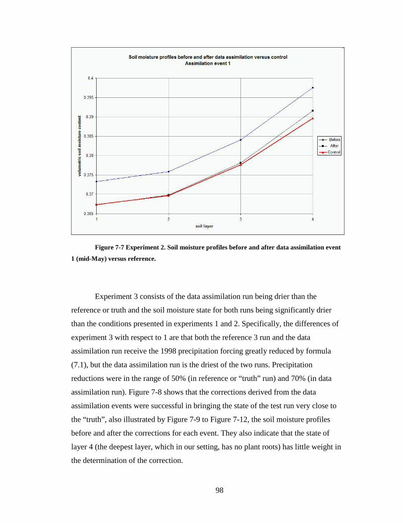
98

Figure 7-7 Experiment 2. Soil moisture profiles before and after data assimilation event

1 (mid-May) versus reference.

Experiment 3 consists of the data assimilation run being drier than the

reference or truth and the soil moisture state for both runs being significantly drier

than the conditions presented in experiments 1 and 2. Specifically, the differences of

experiment 3 with respect to 1 are that both the reference 3 run and the data

assimilation run receive the 1998 precipitation forcing greatly reduced by formula

(7.1), but the data assimilation run is the driest of the two runs. Precipitation

reductions were in the range of 50% (in reference or “truth” run) and 70% (in data

assimilation run). Figure 7-8 shows that the corrections derived from the data

assimilation events were successful in bringing the state of the test run very close to

the “truth”, also illustrated by Figure 7-9 to Figure 7-12, the soil moisture profiles

before and after the corrections for each event. They also indicate that the state of

layer 4 (the deepest layer, which in our setting, has no plant roots) has little weight in

the determination of the correction.

99


line) and data assimilation run (blue line). Second soil layer.

100


1 (mid-May) versus reference (red).


2 (July) versus reference (red).

101


3 (September) versus reference (red).


4 (end of October) versus reference (red).

102

Experiment 4 is similar to 3 except that consists of the reference (“true”) run

being drier than the data assimilation run. As in experiment 3, the soil moisture state

for both runs is significantly drier than the conditions presented in experiments 1 and

2. The differences of experiment 4 with respect to 3 are that the 1998 precipitation

forcing reductions by formula (7.1) are set so that the reference run is the driest one.

Precipitation reductions were in the range of 70% (“truth”) and 50% (data

assimilation). Figure 7-13 shows that the first three corrections derived from the data

assimilation events were successful in bringing the state of the test run very close to

the true state (reference) but no significant change occurred from data assimilation

event 4. Figure 7-14 shows the change produced in the soil moisture profile after data

assimilation event 1, bringing the state very close to the one from control

103


line) and data assimilation run (blue line). Second soil layer.

104


1 (mid-May) versus reference (red).

7.2 Assimilating real data

The experiments that assimilate observed real data have the added challenge

of the presence of differences between the model control run (taken as reference for

the state variables’ trajectories) and observations. That means that the exact

correspondence between variables as given by the reference model run simulating

nature (“truth”) is no longer present (“perfect model” assumption no longer valid).

The impact of the differences between the control run and nature, can be reduced if

the differences are largely unbiased, as such unbiased differences tend to cancel out

as the data assimilation time window is increased, otherwise biased differences can

compromise the results.

105

7.2.1 Assimilating LST from the reference site station

Experiment 5 goes back to the original setting of experiment 1 (wherein an

unaltered 1998 control run is compared with a data assimilation run that received up

to 30% less precipitation) but the data assimilation events in Experiment 5 use the

land surface temperature (LST) observed at the reference site ground station rather

than the control run LST. Since the data assimilation run is receiving 30 percent less

precipitation than the control run, its soil moisture will tend toward being too dry and

its LST too warm during the day, so one expects the assimilation of LST to moisten

the soil and lower the diurnal LST. Figure 7-15 shows the time evolution of the soil

moisture content in model layer 3 for the data assimilation and control run. Only the

third and fourth data assimilation periods (beginning of September and end of

October) yielded the expected positive increase in soil moisture, while the first

assimilation event (in May) had an unexpected impact of the opposite sign.

Taking into account the good correlation of the LST between the reference

station and control run (Figure 6-6), the above experiment was repeated using a

longer data assimilation window. The idea is that, from Figure 6-6, we expect to find

relatively small uncertainties between the behavior of the LST from the control run

and the reference site station and that those uncertainties would be almost unbiased.

Therefore, on a longer time scale, the impact of the unbiased uncertainties should be

reduced or canceled. Figure 7-16 shows the result of this second version of

experiment 5, using a data assimilation window of almost 12 days. This longer

assimilation window resulted in a marked diminution but not elimination of the

unexpected soil moisture decrease in event 1 (mid-May) and great improvement on

events 3 and 4 (September and end of October, respectively). Figure 7-17 shows, for

this case, the soil moisture profiles before and after data assimilation event 1, when

the correction was in the unexpected direction of reducing soil moisture hence

increasing the difference with respect to the control run.

The unexpected soil moisture drying in event 1 (mid-May) suggests that the

LST simulated in the degraded run during this period was not warmer that the LST

observed by the ground station. Hence the apparent absence of bias inferred when

106

comparing the entire year scatter plot of LST from the control run and reference site

station (Figure 6-6) likely masks the presence of significant temporary biases that

change direction during the year. Indeed, Figure 7-18 shows the observed and

simulated LST during the 3 ½ days of data assimilation event 1 and demonstrates that

the LST from the reference site observations is warmer than that simulated by the

control run, so its assimilation will act to reduce the soil moisture rather than correct

(raise) the lowering of soil moisture from the imposed reduction of precipitation. This

is the opposite to what happened in identical twin experiment 1, which assimilated

LST from the control run (which has lower diurnal LST than the test run) and resulted

in increasing (correcting) the soil moisture.

107

Figure 7-15 Experiment 5. Using a cost function of 3 ½ days. Soil moisture content

evolution for the control run (black line) and data assimilation run (blue line). Soil layer 3.

108

Figure 7-16 Experiment 5. Using a cost function of 11 days 20 hrs. Soil moisture content

evolution for the control run (black line) and data assimilation run (blue line). Soil layer 3.

109


1 (mid-May) versus control.

110

Figure 7-18 Experiment 5. Land surface temperature (LST, K) as 1) observed by ground

station (dotted), 2) simulated by control run (red) and 3) simulated by run assimilating the

ground station (blue)

7.2.2 Surface forcing from the North American Land Data

Assimilation System (NLDAS)

In experiments 6 and 7 in this section and experiment 8 in section 7.2.3 the

first run, taken as truth, is the original control, which over the year 1998, reproduced

reasonably well the station LST observations (Figure 6-6). The forcing used for the

assimilation runs in experiments 6, 7 and 8 instead of being different from that in the

control run only in the precipitation, contains differences from the control in all the

forcing fields, which are also expected to cause this run to depart from the reference

trajectory. Specifically, the 1998 forcing data is taken from analyses that combine

atmospheric observations and background states from runs of a mesoscale

atmospheric model (see Mitchell et al., 2004 for an overview of the NLDAS project

and references to companion papers). This NLDAS data was interpolated spatially

from its nearest four grid points to the reference site location and temporally from 1-

111

hour resolution to the 30 minutes resolution matching the reference site station data.

The added challenge then for experiments 6, 7 and 8 is that not only the

precipitation is different from the control but all the seven forcing fields differ

(and by either sign) from what is used for the control run (see section 4.1 for a

listing of the required forcing fields).

Experiment 6 is the first of the NLDAS forcing experiments examined here.

The assimilated observation used in the data assimilation run for experiment 6 is the

LST from the reference site ground station, as in experiment 5 (longer assimilation

window case). Figure 7-19 shows the time evolution of the soil moisture in model soil

layer 3 for these runs.

112


reference site ground station. Soil layer 3 moisture content evolution.

113

Assimilation event 1 had almost no impact and, event 2 produced a small

change. Inspection of the early August period (a non-assimilating period) of the

assimilation run in Figure 7-19 reveals a big departure (of increasing soil moisture)

away from the control run. The magnitude and quickness of the departure strongly

suggests a large precipitation event in the NLDAS forcing that was mostly absent

from the control forcing. Following this early August departure, the subsequent

assimilation events 3 and 4 in late August and October produced strong changes in

the wrong direction, also depicted in the profiles (Figure 7-20 and Figure 7-21).

Given this undesired result, it was deemed wise to test again the assimilation of LST

from the control run, which was the object of experiment 7, described next.


3 (September) versus control.

114


4 (end of October) versus control.

Experiment 7 is similar to 6 in which the data assimilation run is an NLDAS

forced run, but control run LST (rather than ground station observed LST) is

assimilated to derive soil moisture corrections. The time evolution for the soil

moisture in layer 3 (Figure 7-22) and the soil moisture profile for data assimilation

event 1 (Figure 7-23) indicate that the corrections derived are still in the wrong

direction.

This result seems to contradict the idea that in a “perfect model” situation,

assimilating data from the control (“true”) run would be sufficient to bring the soil

moisture states trajectory closer to that of the control run. However, we must

remember that the NLDAS run has completely different forcing from that of the

control run, including not only precipitation but also radiation, wind, air temperature,

pressure and humidity. The data assimilation scheme can find the soil moisture states

that make the test run’s land surface temperature be closest to that of the assimilated

115

LST over the data assimilation window, but since the test run LST is also responding

to a very different direct forcing error (such as radiation), that does not mean making

this run’s LST closer to that of the control run and consequently, does not mean

finding a soil moisture state closer to that of the control run. This is to say that in

experiments 6 and 7 the error in simulated LST may be arising not from soil moisture

error due to wrong precipitation, but from other forcing error. If, for example, the

radiative forcing is overestimated, this will tend to produce a warm LST in the model,

and if we force a correction using only the soil moisture, the soil moisture will be

incorrectly increased in order to cool the LST to counteract the warming of LST from

high radiation forcing.

To illustrate this, Figures 7-24 to 7-26 below show (for a time interval within

assimilation event 1) the model LST behavior with respect to different types of

forcing error compared to the control. First, Figure 7-24 shows the LST time series of

the assimilation run of experiment 7, along with the control run, corresponding to the

two runs given by the red and black curves of Figure 7-23. Figure 7-24 shows that the

LST of the two runs agree closely, despite significant differences (of order .05) in

their soil moisture. Hence, the LST of the control run and the NLDAS-forced

assimilation run of experiment 7 do not differ much despite non-trivial difference in

their soil moisture states. This indicates that the data assimilation scheme has

succeeded in modifying the soil moisture so that the assimilated run has an LST very

similar to that of the observations (control or “truth”). Therefore, the assimilation run

in experiment 7 provides a case where an error in soil moisture is not accompanied by

a significant error in skin temperature. The latter result means that other sources of

LST error besides soil moisture error are operating in the NLDAS-forced runs. As a

reverse confirmation of the latter conclusion, Figure 7-25 shows cooler LST in the

control run than in a non-assimilating test run whose only difference from the control

is the application of slightly less precipitation forcing (and hence less soil moisture,

which results in lower surface latent heat flux and thus warmer LST than the control).

A further illustration of error that emerges in simulated LST due to forcing

errors unrelated to precipitation error, and its attendant soil moisture error, is given in

Figure 7-26. This figure shows warmer LST in the control run compared to a non-

116

assimilating test run in which the only difference from the control is a 30% reduction

of the surface solar insolation. The figure demonstrates that the radiation reduction

alone reduced the LST. Such non-precipitation forcing errors will disrupt and distort

the determination of soil moisture corrections from the contrast between model and

observed LST. In the case of Figure 7-26, an attempt to assimilate the warmer control

run LST into the test run would erroneously decrease the soil moisture in order to

reduce the surface latent heat flux and cause an increase in the simulated LST. This

important result from non-precipitation forcing errors is illuminated further in Section

7.3

117

Figure 7-22 Experiment 7. NLDAS forced run with assimilation of LST from the control

run. Soil moisture evolution for model soil layer 3.

118


1 (mid May) versus control.

119

Figure 7-24 Experiment 7. Land surface temperature (LST) diurnal cycles during the

time window of data assimilation event 1. Shown here are control (red) and NLDAS forced run

(blue dashed line).

Figure 7-25 Soil moisture effect on land surface temperature diurnal cycle by

comparison between model runs in which one of them (blue line) received less precipitation.

120

The precipitation reduced run (blue line) shows greater LST amplitude due to its

reduced soil moisture content.

Figure 7-26 Solar radiation effect on land surface temperature (LST) diurnal cycle by

comparison between model runs in which one of them received less solar radiation forcing

(70%). The radiation reduced run (blue line) shows smaller LST amplitude.

7.2.3 Assimilating LST from the GOES satellite

GOES satellites provide the feasibility of retrieving hourly LST on a

continental scale as discussed in section 4.3.. This would make possible the

assimilation of LST in order to correct soil moisture initial condition in land surface

models.

Experiment 8 differs from 7 and 6 by the fact that the assimilated LST comes

from the GOES LST retrieval of section 4.3 temporally and spatially interpolated in

the same form to the reference site as it was done with the NLDAS forcing. Also,

since the temporal availability of this GOES LST data is sparse, data assimilation

events were restricted to situations when at least six consecutive hours of GOES LST

121

data were available and the data assimilation time windows were restricted to this

availability. In this data set, the longest time series of consecutive hourly GOES LST

was 11 hours. Such data assimilation windows are too small to be visualized as two

different marks signaling the beginning and end in a figure depicting a yearly time

scale. Thus each mark labeled “DA event” in Figure 7-27 are actually two marks

(representing the beginning and end of the data assimilation window).

In experiment 8 the evolution third layer soil moisture (Figure 7-27) shows

that the data assimilation events alter the trajectory of the data assimilation run (blue

line) considerably in the direction of the control run (black line), as can be seen by

comparison with the NLDAS forced run without data assimilation (dotted red).

Nevertheless, the assimilation run (blue line) quickly departs from the control run

(black line) in between data assimilation events during the moisture charged, rainy

part of the year (April-May) suggesting the strong differences in forcing and the

limited memory of the system under these conditions. The presence of 1-2 degrees

Kelvin warm biases (not shown) in the GOES land surface temperature are, to a

certain extent, offset by the high surface solar insolation biases (not shown) imposed

on the model land surface temperature under NLDAS forcing, causing the soil

moisture corrections to be in the right direction (before and after profiles Figure 7-27

to Figure 7-32).

122

Figure 7-27 Experiment 8. Soil moisture content evolution for the control run (black),

the NLDAS forced GOES LST data assimilation run (blue) and the NLDAS forced run without

data assimilation (dotted red). Third soil layer.

123


1 (early April) versus control.


2 (mid April) versus control.

124


3 (late April) versus control.


4 (early September) versus control.

125


5 (mid September) versus control.

7.3 Conclusions from the ideal and real data assimilation

experiments.

In summary, we have shown that the assimilation of LST (a variable that in

principle can be observed from geostationary satellites and/or from ground stations)

to improve the initialization of soil moisture (a variable that is generally unobserved

but which influences the forecasts) is feasible if the surface forcings other than

precipitation are known with great accuracy and the model is not biased.

With a realistic model and detailed observations of surface forcing, we were

able to generate realistic LST and soil moisture for a given station. With this model,

and accurate forcing besides precipitation, we did succeed in improving substantially

the initial soil moisture by assimilating LST, even if the precipitation driving the soil

model was either substantially overestimated or underestimated.

126

However, when we used surface forcing estimated from NLDAS, which have

substantial uncertainties and probably significant biases, in both precipitation and

non-precipitation forcing like radiative fluxes, we found that the results were not

good (Experiment 7). Essentially, the assimilation system, as designed, was able to

change the model LST in order to reproduce the assimilated LST by modifying the

soil moisture. In this case, however, the origin of the LST error in the model was not

the precipitation forcing and soil moisture but the non-precipitation forcing. This

indicates that the problem of soil moisture initialization is not sufficiently constrained

by the observations of LST alone. Possible approaches to deal with this important

problem are briefly discussed in the final chapter.

127

Chapter 8

Conclusions

Land surface models are used to compute energy and water fluxes between the

land and the atmosphere. A very important requirement of these models is the initial

values of soil moisture, which is difficult to measure over large areas. Good quality

soil moisture measurements for the above purposes involve planting devices into the

soil at several depths between 0 and 1 meter or more. The problems are the large

areas needing measurement and the spatial and temporal variations of soil moisture.

Through physics (Chapters 2 and 3), land surface models couple the soil

moisture with other variables (such as low-level air temperature and relative

humidity, land surface temperature, and sensible, latent and ground heat fluxes at the

surface). Some of those (like land surface temperature) are easier to remotely measure

than the soil moisture itself. Variational techniques allow the solution of the inverse

problem of using land surface models to determine the soil moisture content from

information on other variables (Chapter 2). The land surface model quality is

important. We showed in Chapter 5 and in section 6.2 the several components of this

project that led to improvements in either the model or in its numerical properties,

leading to more efficient minimization algorithms.

The main results of assimilating LST in order to estimate the initial soil

moisture were presented in Chapter 7. The “perfect model” scenarios (such as the

twin experiment, section 7.1) work very well (Figure 7-1) when only errors in the soil

moisture content are affecting the observed variable (LST). In this sense, the

methodology has succeeded: if the other surface forcings are accurate, the

assimilation of LST succeeds in substantially improving the soil moisture.

However, when we used surface forcing fields that would be available

operationally, such as those from the NLDAS, the results were not good. This is

because when other factors (such as radiative fluxes) influence the observed variable

(LST), the influence from the soil moisture content is not easily recovered. The

method successfully modifies the soil moisture in such a way as to make the model

128

LST follow the observed LST during the assimilation window, but this may not be

desirable when the errors in the non-precipitation forcings are large enough to impact

the LST at least as much as the errors in the soil moisture.

Future developments suggested by this work indicate the need to observe and

use more variables in combination leading to isolating the effects of the soil moisture

content on this new set of observations. Variational techniques can also be used to

optimize the model (e.g. model parameters) but need reliable observations related to

model output in order to adjust the model to reproduce their behavior. There have

been recent developments in data assimilation that also offer considerable promise for

attacking this problem. In particular, a new method known as 4-Dimensional

Ensemble Kalman Filter (Hunt et al, 2004) has several advantages of both 4D-Var

and Ensemble Kalman Filter (EnKF). Like other EnKF approaches, it does not

require the linear tangent or adjoint models, and it solves the assimilation problem

directly, not iteratively. EnKF would allow a simple inclusion of error correlations

between different variables and forcings, thus reducing the problem of spurious

corrections of soil moisture to account for errors due to other forcings that we found

when using real data. EnKF can also be modified to estimate model deficiencies. 4D

EnKF shares the ability of 4D-Var of assimilating observations at their correct time

within an assimilation window, at the end of which the system provides not only an

analysis but also an analysis error covariance. We believe that the combination of

using more observations and such a flexible approach can achieve the desired goal of

initializing soil moisture more accurately and thus improving forecasts.

129

Appendices

Appendix A: Limitations to the convergence of a finite-

difference approximation scheme to the derivative in the

presence of round-off errors.

A finite-differences estimate of the first derivative of a function calculated

with a certain computer precision carries two major sources of error: the truncation

error and the condition error (Gill et al., 1981). It will be shown that in this case, the

truncation error cannot be arbitrarily diminished by decreasing the differences

interval, h, because the uncertainties in the function computation are being magnified

by a factor of h

1 in the finite differences formula.

The truncation error from a finite-differences estimate of the first derivative

can be derived from the Taylor series expansion

( ) ( ) ( ) ( )ξfhxf hx fhxf ′′+′+=+ 2

2

1

yielding

( ) ( ) ( ) ( )ξfhh

xfhxfxf ′′−−+=′ 2

2

1

indicating that the error in the approximation,

( ) ( ) ( )h

xfhxfxf

−+≈′

will be in the magnitude of ( )ξfh ′′2

1, where ξ is between x and x + h.

The condition error is calculated from the rounding errors in the evaluation of

the function f itself at machine precision in the numerator of the finite differences

formula, this rounding error is of the order of ( )εxf , where ε is the relative

130

precision of the computer calculation of f so, the condition error in the finite

differences formula will be of the order of ( )h

xf ε, and this becomes arbitrarily large

if h becomes arbitrarily small. Therefore, the finite differences approximation error

cannot be arbitrarily reduced by reducing the difference interval arbitrarily when the

function being differentiated is computed with round-off errors.

131

Bibliography

Baer, F., and Simons, T.J., 1970: Computational stability and time truncation of

coupled linear equations with exact solutions. Monthly Weather Review, Vol.

98, 665-679

Bastidas, L. A., H.V. Gupta, S. Sorooshian, W.J. Shuttleworth and Z.L. Yang

"Sensitivity Analysis of a Land Surface Scheme using Multi-Criteria

Methods", Journal of Geophysical Research, Vol. 104, No D16, p. 19,481-

19,490, 1999.

Bastidas, L. A., H. V. Gupta, and S. Sorooshian, Bounding parameters of land surface

schemes with observational data, in Observations and Modeling of the Land

Surface Hydrological Processes, V. Lakshmi, J. Albertson & J. Schaake,

Editors, Water Science and Application Volume 3, p. 65-76, American

Geophysical Union, 2001.

Bastidas, L. A., H. V. Gupta, and S. Sorooshian, Parameter, Structure and

Performance Evaluation for Land Surface Models, in Advances in the

Calibration of Watershed Models, Q. Duan, H. V. Gupta, S. Sorooshian, A.

Rousseau, and R. Turcotte, Editors, AGU, 2002.

Beljaars, A. C. M., Viterbo, P., Miller, M.J., Betts, A., 1996: The Anomalous

Rainfall Over The United States During July 1993: Sensitivity To Land

Surface Parameterization And Soil Moisture Anomalies. Monthly Weather

Review, Vol. 124, No. 3, March 1996.

Bell, S., 1994: Mesoscale Assimilation Of Moisture Parameters. Hirlam 3 Workshop

On Analysis, Initialization And Data Assimilation. Norrkoping 23-24

February 1994.

Berbery, E. H., K. E. Mitchell, S. Benjamin, T. Smirnova, H. Ritchie, R. Hogue and

E. Radeva 1999: Assessment of land surface energy budgets from regional

and global models. J. Geophys. Res., 104, D16, 19,329-19,348.

132

Berbery, E. H., Y. Luo, K. E. Mitchell, and A. K. Betts (2003), Eta model estimated

land surface processes and the hydrological cycle of the Mississippi basin, J.

Geophys. Res., 108(D22), 8852, doi:10.1029/2002JD003192.

Betts, A. K., Ball, J.H., 1995: The Fife Surface Diurnal Cycle Climate. Journal Of

Geophysical Research, Vol. 100, No. D12, 25,679-25,693, December 20,

1995.

Betts, A. K., Ball, J.H., Beljaars, A. C. M., Miller, M. J., Viterbo, P., 1996: The Land

Surface-Atmosphere Interaction: A Review Based On Observational and

Global Modeling Perspectives. Journal of Geophysical Research, Vol. 101,

No. D3, 7209-7225.

Betts, A. K., Hong, S.-Y., Pan, H.-L., 1996: Comparison Of NCEP-NCAR Reanalysis

With 1987 Fife Data. Monthly Weather Review, Vol. 124, No. 7, July 1996.

Betts, A. K., Ball, J.H., 1997: Fife Surface Climate and Site-Average Dataset 1987-

89. Journal of the Atmospheric Sciences, Vol. 55, No. 7, pp. 1091–1108.

Betts, A. K., Chen F., Mitchell, K.E., Janjic, Z., 1997: Assessment of the Land-

Surface and Boundary-Layer Models in Two Operational Versions of the

NCEP Eta Model Using Fife Data. Monthly Weather Review. Vol. 125. 2896-

2916.

Betts, A. K., Viterbo, P., Wood, E., 1997: Surface Energy And Water Balance For

The Arkansas-Red River Basin From The ECMWF Analysis. Submitted To

Journal Of Climate.

Betts, A. K., Viterbo, P., Beljaars, A. C. M., 1998: Comparison Of The Land-Surface

Interaction In The ECMWF Reanalysis Model With The 1987 Fife Data.

Monthly Weather Review, Vol. 126, 186-198, January 1998.

Bouttier, F., 1994. Soil Moisture Assimilation At Meteo-France. Hirlam 3 Workshop

On Analysis, Initialization And Data Assimilation. Norrkoping 23-24

February 1994.

133

Bouttier, F., J.-F. Mahfouf, J. Noilhan, 1993-A: Sequential Assimilation of Soil

Moisture from Atmospheric Low-Level Parameters. Part I: Sensitivity and

Calibration Studies. Journal of Applied Meteorology, Vol. 32, 1335-1351.

Bouttier, F., J.-F. Mahfouf, J. Noilhan, 1993-B: Sequential Assimilation of Soil

Moisture from Atmospheric Low-Level Parameters. Part II: Implementation

in a Mesoscale Model. Journal of Applied Meteorology, Vol. 32, 1352-1364.

Calvet, J-C., Noilhan, J., Bessemoulin, P., 1998: Retrieving The Root-Zone Soil

Moisture From Surface Soil Moisture Or Temperature Estimates: A

Feasibility Study Based On Field Measurements. Journal Of Applied

Meteorology, Vol. 37, 371-386, April 1998.

Campbell, G. S., A simple method for determining unsaturated conductivity from

moisture retention data, Soil Sci., 117, 311-314, 1974.

Cosgrove, B. A., et al. (2003), Real-time and retrospective forcing in the North

American Land Data Assimilation System (NLDAS) project, J. Geophys.

Res., 108(D22), 8842, doi:10.1029/2002JD003118.

Chen, F., and K. Mitchell, 1998: Using the GEWEX/ISLSCP Forcing Data to

Simulate Global Soil Moisture Fields and Hydrological Cycle for 1987-1988.

Submitted to the Journal Of The Meteorological Society Of Japan, June 30,

1998 (Accepted).

Chen, F., K. Mitchell, J. Schaake, Y. Xue, H.-L. Pan, V. Koren, Q.-Y. Duan, M. Ek

and A. Betts, 1996: Modeling Of Land-Surface Evaporation by Four Schemes

and Comparison with Fife Observations. Journal of Geophysical Research,

Vol. 101, No. D3, 7251-7268.

Chen, F., Z. Janjic and K. Mitchell, 1997: Impact of Atmospheric Surface-Layer

Parameterization in the New Land-Surface Scheme of the NCEP Mesoscale

Eta Model. Boundary-Layer Meteorology, v 85, no. 3, 391-422.

Cohn, S. E., 1997: An Introduction To Estimation Theory. Journal Of The

Meteorological Society Of Japan.

134

Cohn, S. E., Todling, R., 1995: Approximate Data Assimilation Schemes For Stable

And Unstable Dynamics. Journal Of The Meteorological Society Of Japan.

(Accepted)

Cosby, B.J., Et Al., 1984: A Statistical Exploration Of The Relationships Of Soil

Moisture Characteristics To The Physical Properties Of Soils. Water

Resources Research, Vol. 20, No. 6, 682-690, June 1984.

Courtier, P. Et Al., 1993: Important Literature On The Use Of Adjoint, Variational

Methods And The Kalman Filter In Meteorology. Tellus, 45a (1993) 5, 342-

357.

Courtier, P., 1997: Variational Methods. Journal Of The Meteorological Society Of

Japan, Vol. 75, No. 1b. 211-218, 1997.

Deardorff, J. W. 1972: Parameterization of the planetary boundary layer for use in

general circulation models. Mon. Wea. Rev., 100, 93-106.

Deardorff, J. W. 1978: Efficient prediction of ground surface temperature and

moisture with inclusion of a layer of vegetation. J. Geophys. Res., 83, 1889-

1903.

Derber, J. C., 1987: Variational Four-Dimensional Analysis Using Quasi-Geostrophic

Constraints. Monthly Weather Review, Vol. 115 No. 5. 998-1008.

Dirmeyer, P.A., 1997: Assessing GCM Sensitivity to Soil Wetness Using GSWP

Data. Cola Report No. 47. Center For Ocean-Land-Atmosphere Studies.

September 1997.

Dirmeyer, P.A., Zeng, F., 1997: A Two Dimensional Implementation of the Simple

Biosphere (Sib) Model. Cola Report. Center For Ocean-Land-Atmosphere

Studies. September 1997.

Dirmeyer, P.A.. et al., 2002: see International GEWEX Project Office, 2002 GSWP-

2.

135

Duan, Q., Sorooshian, S., Gupta, V., 1992: Effective And Efficient Global

Optimization For Conceptual Rainfall- Runoff Models. Water Resources

Research, Vol. 28. No. 4. 1015-1031, April 1992.

Ek, M. And L. Mahrt, 1991: A One-Dimensional Planetary Boundary Layer Model

with Interactive Soil Layers and Plant Canopy. Users Guide Version 1.0.4.

College of Oceanic and Atmospheric Sciences, Strand Agriculture Hall, Rm.

326, Oregon State University Corvallis, Oregon 97331-2209 USA.

Ek, M. B., K. E. Mitchell, Y. Lin, E. Rogers, P. Grunmann, V. Koren, G. Gayno, and

J. D. Tarpley (2003), Implementation of Noah land surface model advances in

the National Centers for Environmental Prediction operational mesoscale Eta

model, J. Geophys. Res., 108(D22), 8851, doi:10.1029/2002JD003296.

Entekhabi, D., Nakamura, H., Njoku, E.G., 1994: Solving The Inverse Problem For

Soil Moisture And Temperature Profiles By Sequential Assimilation Of

Multifrequency Remotely Sensed Observations. IEEE Transactions On

Geoscience And Remote Sensing, Vol. 32, No. 2, 438-447. March 1994.

Farouki, O.T.,1986: Thermal Properties Of Soils. Series On Rock And Soil

Mechanics, Vol. 11, Trans Tech, 136 Pp.

Garratt, J. R., 1993: Sensitivity of Climate simulations to Land-Surface and

Atmospheric Boundary-Layer Treatments-A Review. Journal Of Climate,

Vol. 6, 419-449.

Giering, R. And T. Kaminski, 1996: Recipes for Adjoint Code Construction. Tech.

Report 212, Max-Planck-Institut Fur Meteorologie.

Giering, R., 1997: Tangent Linear and Adjoint Model Compiler, Users Manual. Max

-Planck - Institut Fur Meteorologie.

Gill, P. E., W. Murray and M. H. Wright, 1981: Practical Optimization. Academic

Press, New York.

Gutman, G., 1994: Global Data on Land Surface Parameters From NOAA AVHRR

For Use In Numerical Climate Models. Journal Of Climate, Vol. 7, 669-680.

May 1994.

136

Hicks, B.B., Deluisi, J.J., Matt, D. R., 1996: The NOAA Integrated Surface

Irradiance Study (Isis)-A New Surface Radiation Monitoring Program.

Bulletin Of The American Meteorological Society, Vol. 77, No. 12, December

1996. 2857-2864.

Hirlam 3 Workshop On Analysis, Initialization And Data Assimilation. Norrkoping

23-24 February 1994.

Hunt, B.R. , E. Kalnay, E.J. Kostelich, E. Ott, D.J. Patil, T. Sauer, I. Szunyogh, J.A.

Yorke, and A.V. Zimin, 2004: Four-Dimensional Ensemble Kalman Filtering.

Tellus 56A, 273-277.

International GEWEX Project Office, 2002: GSWP-2: The Second Global Soil

Wetness Project Science and Implementation Plan. IGPO Publication Series

No. 37, 65 pp.

Jacquemin, B. and J. Noilhan, 1990: Sensitivity study and validation of a land surface

parameterization using the Hapex-Mobilhy data set. Boundary Layer

Meteorology, 52: 93-134.

Jarviz, P. G., 1976: The interpretation of the variation in leaf water potential and

stomatal conductance found in canopies in the field. Philosophical

Transactions of the Royal Society of London B, 273, 593-610.

Jaervinen, Heikki, 1993: A direct conversion of model algorithms to their adjoints

exemplified with a barotropic atmospheric model. Helsinki, Finland,

University of Helsinki, Department of Meteorology, 1993. 41 pp. 1993.

Johansen, O., 1975: Thermal Conductivity Of Soils. Ph.D. Thesis, University Of

Trondheim.w130)h

Jones, A. S., I. C. Guch, and T. H. Vonder Haar, 1998: Data Assimilation Of

Satellite-Derived Heating Rates As Proxy Surface Wetness Data Into A

Regional Atmospheric Mesoscale Model. Part I: Methodology. Monthly

Weather Review, Vol. 126, 634-645.

Kalnay, Eugenia, 2003: Atmospheric Modeling, Data Assimilation and Predictability.

Cambridge University Press, 341 pages.

137

Kapitza, H., 1991: Numerical Experiments With The Adjoint Of A Nonhydrostatic

Mesoscale Model. Monthly Weather Review, Vol. 119, December 1991,

2993-3011.

Koren, V., J. Schaake, K. Mitchell, Q.-Y. Duan, F. Chen and JM Baker, 1999-A: A

parameterization of snowpack and frozen ground intended for NCEP weather

and climate models. Journal Of Geophysical Research. Vol. 104, no. D16, pp.

19569-19585.

Koren, V., Q.-Y. Duan and J. Schaake, 1999-B: Validation of a snow-frozen ground

parameterization of the Eta model. Preprint AMS 14 Hydrology Conference,

10-15 January 1999, Dallas TX, Paper J1.3 .

Koster, R. D., and M. J. Suarez, 2003: Impact of Land Surface Initialization on

Seasonal Precipitation and Temperature Prediction. J. Hydrometeorlogy, 4,

408-423.

LeDimet, F. X., and O. Talagrand, 1986: Variational algorithms for analysis and

assimilation of meteorological observations. Tellus 38a , 97-110.

Lewis, J. M., J. C. Derber, 1985: The Use Of Adjoint Equations To Solve A

Variational Adjustment Problem With Advective Constraints. Tellus 37a, 309-

322.

Liang, X., E.F. Wood, D.P. Lettenmaier et al., The project for intercomparison of

land-surface parameterization schemes (PILPS) phase-2c Red-Arkansas river

basin experiment: 2. Spatial and temporal analysis of energy fluxes, Global

and Planetary Change, 19(1-4), 137-159, 1998.

Lohmann, D., et al. (2004), Streamflow and water balance intercomparisons of four

land surface models in the North American Land Data Assimilation System

project, J. Geophys. Res., 109, D07S91, doi:10.1029/2003JD003517.

Luo, L. et al., 2003-A: Effects of Frozen Soil on Soil Temperature, Spring

Infiltration, and Runoff: Results from the PILPS 2(d) Experiment at Valdai,

Russia. Journal of Hydrometeorology: Vol. 4, No. 2, pp. 334–351.

138

Luo, L., et al., 2003-B: Validation of the North American Land Data Assimilation

System (NLDAS) retrospective forcing over the southern Great Plains, J.

Geophys. Res., 108(D22), 8843, doi:10.1029/2002JD003246.

Manabe, S., 1969: Climate and the circulation, I. The atmospheric circulation and the

hydrology of the earth's surface. Mon. Wea. Rev., 97, 739-774.

Mahfouf, J.-F., 1990a: A Numerical Simulation Of The Surface Water Budget During

Hapex-Mobilhy. Boundary Layer Meteorology, 53: 201-222, 1990.

Mahfouf, J.-F., 1990b: A Variational Assimilation Of Soil Moisture In

Meteorological Models. WMO International Symposium On Assimilation Of

Observations In Meteorology And Oceanography. Clermont-Ferrand, France,

July 1990.

Mahfouf, J.-F., 1991: Analysis Of Soil Moisture From Near-Surface Parameters: A

Feasibility Study. Journal Of Applied Meteorology, Vol. 30 1534-1547.

Mahfouf, J-F. and P. Viterbo, 1996: Land Surface Assimilation. Proceedings Of

Seminar On Data Assimilation. ECMWF. 2-6 September 1996. 319-347.

Mahrt, L. and M. Ek., 1984: The influence of atmospheric stability on potential

evaporation. Journal Of Climate and Applied Meteorology, Vol. 23, no. 2,

222-234.

Mahrt, L., Pan, H. L., 1984: A Two-Layer Model Of Soil Hydrology. Boundary-

Layer Meteorology, 29, 1-20

Marshall, C.H., 1998: Evaluation Of The New Land-Surface And Planetary Boundary

Layer Parameterization Schemes In The NCEP Mesoscale Eta Model Using

Oklahoma Mesonet Observations. M.Sc. Thesis. University of Oklahoma.

Marshall, C. H., K. C. Crawford, K. E. Mitchell and D. J. Stensrud. 2003: The Impact

of the Land Surface Physics in the Operational NCEP Eta Model on

Simulating the Diurnal Cycle: Evaluation and Testing Using Oklahoma

Mesonet Data. Weather and Forecasting, 18, 748–768.

139

Mitchell, K. E., 1994: GCIP Initiatives In Operational Mesoscale Modeling And Data

Assimilation At NMC. Preprint In The AMS Fifth Symposium On Global

Change Studies, 23- 28 January 1994, Nashville TN, Paper 6.8, Pp.192-198.

Mitchell, K. E., J. Schaake, D. Tarpley, F. Chen, Y. Lin, M. Baldwin, E. Rogers, G.

Manikin, A. Betts, Z. Janjic, Q.-Y. Duan, V. Koren, 1999-A: Recent GCIP

Advancements in Coupled Land-Surface Modeling and Data Assimilation in

the NCEP Mesoscale Eta Model. Preprint AMS 14 Hydrology Conference, 10-

15 January 1999, Dallas TX, Paper 4B.1 .

Mitchell, K., P. Houser, E. Wood, J. Schaake, D. Tarpley, D. Lettenmaier, W.

Higgins, C. Marshall, D. Lohmann, M. Ek, B. Cosgrove, J. Entin, Q. Duan, R.

Pinker, A. Robock, F. Habets and K. Vinnikov, 1999-B: GCIP Land Data

Assimilation System (LDAS) Project Now Underway. GEWEX News, Vol. 9,

No. 4, November 1999, pp. 3-6, IGPO, Silver Spring, MD.

Mitchell, K. E., et al. (2004), The multi-institution North American Land Data

Assimilation System (NLDAS): Utilizing multiple GCIP products and

partners in a continental distributed hydrological modeling system, J.

Geophys. Res., 109, D07S90, doi:10.1029/2003JD003823.

Namias, J., 1958: Persistence of mid-tropospheric circulations between adjacent

months and seasons. The atmosphere and sea in motion (Rossby memorial

volume). B. Bolin, Ed., New York: Rockefeller Inst.; Oxford University Press,

240-248

Nash, S. and A. Sofer, 1996: Linear and Nonlinear Programming. McGraw-Hill Co.

Inc., 692 pp.

Navon, I. M., X. Zou, J. Derber and J. Sela, 1992: Variational Data Assimilation with

an Adiabatic version of the NMC Spectral Model. Monthly Weather Review,

Vol. 120, No. 7 1433-1446.

Noilhan J. and Planton, S.: 1989, ‘A Simple Parameterization of Land Surface

Processes for Meteorological Models’, Mon. Wea. Rev. 117, 536–549.

140

Ottle, C., Vidal-Madjar, D., 1994: Assimilation Of Soil Moisture Inferred From

Infrared Remote Sensing In A Hydrological Model Over The Hapex-Mobilhy

Region. Journal Of Hydrology 158 (1994) 241-264.

Pan, H-L, 1990: A Simple Parameterization Scheme Of Evapotranspiration Over

Land For The NMC Medium-Range Forecast Model. Monthly Weather

Review, Vol. 118 No. 12, 2500-2512.

Pan, H-L, L. Mahrt, 1987: Interaction Between Soil Hydrology And Boundary-Layer

Development. Boundary-Layer Meteorology, 38, 185-202.

Peters-Lidard, C. D., E. Blackburn, X. Liang, E. F. Wood, 1998: The Effect Of Soil

Thermal Conductivity Parameterization On Surface Energy Fluxes And

Temperatures. Journal of the Atmospheric Sciences, Vol. 55, 1209-1224.

Peters-Lidard, C.D., Zion, M.S., Wood, E.F., 1997: A Soil-Vegetation-Atmosphere

Transfer Scheme For Modeling Spatially Variable Water And Energy Balance

Processes. Journal Of Geophysical Research, Vol. 102, No. D4, 4303-4324,

February 27, 1997.

Pinker, R., I. Laszlo, Y. Wang And J. D. Tarpley, 1996: GCIP Goes-8 Shortwave

Radiation Budgets: Validation Activity. Second International Scientific

Conference On Global Energy And Water Cycle, 245- 249.

Pinker, R. T., et al. (2003), Surface radiation budgets in support of the GEWEX

Continental-Scale International Project (GCIP) and the GEWEX Americas

Prediction Project (GAPP), including the North American Land Data

Assimilation System (NLDAS) project, J. Geophys. Res., 108(D22), 8844,

doi:10.1029/2002JD003301.

Robock, A. Et Al., 1996: Soil Moisture Parameterization In GCMS And Evaluation

of AMIP Simulations. Submitted To Earth Interactions. April 1996.

Schaake, J.C., Et Al., 1996: Simple Water Balance Model For Estimating Runoff At

Different Spatial And Temporal Scales. Journal Of Geophysical Research,

Vol. 101, No. D3, 7461-7475.

141

Shanno, D. F., 1978: Conjugate gradient methods with inexact linesearch. Math.

Operations Res., 3, 244-256.

Shao, Y., Henderson-Sellers, A., 1996: Validation Of Soil Moisture Simulation In

Land-Surface Parameterization Schemes With Hapex Data. Global And

Planetary Change, 13 (1996) 11-46.

Smith, B., Et Al. 1994: Initialization Of Soil-Water Content In Regional-Scale

Atmospheric Prediction Models. Hirlam 3 Workshop On Analysis,

Initialization And Data Assimilation. Norrkoping 23-24 February 1994.

Sorooshian, S., Duan, Q., Gupta, V., 1993: Calibration Of Rainfall- Runoff Models:

Application Of Global Optimization To The Sacramento Soil Moisture

Accounting Model. Water Resources Research, Vol. 29. No. 4. 1185-1194,

April 1993.

Stull, R., 1988: An Introduction To Boundary- Layer Meteorology. Kluwer,

Massachusetts, 666 Pp.

Tarpley, J. D., I. Laszlo And R. T. Pinker, 1996: Experimental Goes Short-Wave

Radiation Budget For GCIP. Second International Scientific Conference On

Global Energy And Water Cycle, 284-285.

Todling, R., Cohn, S. E., Sivakumaran, N.S., 1997: Suboptimal Schemes For

Retrospective Data Assimilation Based On The Fixed-Lag Kalman Smoother.

Dao Office Note 97-Nn. Nasa. February 1997.

Van Den Hurk, B. J. J. M., Et Al., 1997: A New Methodology For Assimilation Of

Initial Soil Moisture Fields In Weather Prediction Models Using Meteostat

And NOAA Data. Journal Of Applied Meteorology V. 36 N. 9, 1271- 1283.

Viterbo, P. And C.M. Beljaars, 1995: An Improved Land Surface Parameterization

Scheme In The ECMWF Model And Its Validation. Journal Of Climate. Vol.

8, 2716-2748.

Viterbo, P. And Illari, L. 1994: The Impact Of Changes In The Runoff Formulation

Of A General Circulation Model On Surface And Near-Surface Parameters.

Journal Of Hydrology. Vol. 155, no. 3 / 4 , 325-336.

142

Viterbo, P., 1996: The Representation Of Surface Processes In General Circulation

Models. Ph.D. Thesis, University Of Lisbon, 201 Pp.

Viterbo, P., Courtier, P., 1995: The Importance Of Soil Water For Medium-Range

Weather Forecasting. Implications For Data Assimilation. Proceedings Of

WMO Workshop On Imbalances Of Slowly Varying Components Of

Predictable Atmospheric Motions. Beijing, 1995.

Vukicevic, T. and R. Errico, 1993: Linearization and adjoint of parameterized moist

adiabatic processes. Tellus, 45a, 493-510.

Wu, X., W. P. Menzel, and G. S. Wade (1999), Estimation of sea surface

temperatures using GOES-8/9 radiance measurements, Bull. Am. Meteorol.

Soc., 80, 1127– 1138.

Zou, X., I. M. Navon and J. Sela, 1993: Variational data assimilation with moist

threshold processes using the NMC Spectral Model. Tellus, 45a, 370-387.

Zupanski, D., 1993: The effects of discontinuities in the Betts-Miller cumulus

convection scheme on four-dimensional variational data assimilation. Tellus,

45a, 511-524.

Zupanski, D., 1996: A general weak constraint applicable to operational 4DVAR data

assimilation systems. Monthly Weather Review, Vol. 125, 2274-2292.

Zupanski, D., Mesinger, F., 1995: Four-Dimensional Variational Assimilation Of

Precipitation Data. Monthly Weather Review, Vol. 123, No. 4, 1112-1127.

April 1995.Zupanski, M., 1993a: Regional Four-Dimensional Variational

Data Assimilation In A Quasi-Operational Forecasting Environment. Monthly

Weather Review, Vol. 121, No. 8, Pp.2396-2408. August 1993.

Zupanski, M., 1993b: A Preconditioning Algorithm For Large-Scale Minimization

Problems. Tellus , 45a, 478-492.

Zupanski, M., 1996: A Preconditioning Algorithm for Four-Dimensional Variational

Data Assimilation. Monthly Weather Review, Vol. 124, 2562-2573.

November 1996.

Documents

ABSTRACT - atmos.umd.eduekalnay/dissertations/Grunmann... · ABSTRACT Title: VARIATIONAL DATA ASSIMILATION OF SOIL MOISTURE INFORMATION ... Dusanka Zupanski and Prof. Ferdinand Baer