Merger Activity In Industry Equilibrium∗

Theodosios Dimopoulos† Stefano Sacchetto††

Abstract

We study the effects of mergers and acquisitions on industry dynamics. We develop an

infinite horizon model of a competitive industry, which features mergers, entry, exit, and in-

vestment by heterogeneous firms. Merger synergies arise from improvements in productivity

and cost efficiencies. We characterize the time-series and cross-sectional evolution of firm

productivities and merger opportunities in a rational expectations equilibrium. Consistent

with the empirical evidence, our model generates procyclical entry and merger activity, as

well as counter-cyclical exit. The presence of a merger market induces higher entry rates

and lower exit rates, reduces the counter-cyclicality of exit, and increases the mean and

variance of the cross-sectional distribution of firm-level productivities. While entry and

exit induce the mean productivity to be counter-cyclical, this pattern is reversed when the

possibility of mergers is taken into account.

JEL Classifications: D21, D92, E22, E32, G34, L11

Keywords: Mergers, Industry Equilibrium

∗First draft, please do not cite without the authors’ permission. All remaining errors are our responsibility.† Swiss Finance Institute, and University of Lausanne. Address: Institut de banque et finance (IBF), HEC

Lausanne, Universite de Lausanne, Extranef 237, 1015, Lausanne, Switzerland. Phone: +1-41-21-692-3398.Email: Theodosios.Dimopoulos@unil.ch.

†† Tepper School of Business, Carnegie Mellon University. Address: Tepper School of Business, 5000Forbes Avenue, Pittsburgh, PA 15213, USA. Phone:+1-412-268-8832. E-mail: sacchetto@cmu.edu.

1. Introduction

Mergers and acquisitions (M&A) have a significant impact on the evolution of industries.

They account for a large fraction of firm turnover, facilitate the redeployment of capital to

productive uses, and accelerate the transmission of new technologies among firms. For the

parties involved, M&As represent complex investment decisions, as companies weigh the

value of the synergies generated in a given deal against future takeover opportunities.

Figure 1 highlights two stylized facts about aggregate merger and exit activity.1 First,

M&As account for a large portion of firm turnover: between 1981 and 2010, approximately

4.5% of active public firms merged in a given year, while the exit rate due to poor perfor-

mance was 3.7%. Second, merger activity is procyclical, which has been documented by a

large body of empirical work (e.g., Andrade, Mitchell, and Stafford, 2001; Harford, 2005),

whereas exit is counter-cyclical (Campbell, 1998).

What determines the joint dynamics of mergers, exit, and entry over the business cycle?

What are the effects of merger activity on the evolution of the cross-section of firms in the

industry? To answer these questions, we develop an infinite horizon model of a competitive

industry populated by firms with heterogeneous productivities. In each period, potential

entrants decide whether to pay an entry cost and invest in productive capital. Incumbents

choose the capital stock and decide whether to exit the industry. They also participate in

the market for corporate control, by which potential takeover matches are formed. Merger

synergies are generated by improvements in productivity and reductions in the fixed costs of

production. Conditional on deciding to merge, the terms of exchange are decided by Nash

bargaining between the two firms, and a fixed merger implementation cost is incurred. The

bargaining framework accounts endogenously for potential future takeover opportunities,

should one of the parties refuse to accept the deal. Because firms face persistent aggregate

and idiosyncratic productivity shocks, they are heterogeneous in terms of both the current

synergies and future takeover opportunities.

In the model, potential entrants choose to exercise their entry option whenever a signal

1M&A activity and exit rates are measured by the fraction of public firms in CRSP that are delisted in agiven year because of a merger (Figure 1a) or poor performance (Figure 1b), respectively. See Appendix Afor a detailed description of the delisting codes used to measure mergers and exit activity. These rates arepartly affected by the fact that CRSP coverage increased substantially in 1962 to include AMEX firms andin 1972 to include NASDAQ firms.

2

about their own future productivity exceeds a certain threshold. Similarly, incumbents

leave the industry when their idiosyncratic productivity drops below an exit threshold.

Conditional on being matched, incumbent firms agree to merge whenever the productivity

and cost synergies are high enough to compensate for the merger implementation costs.

We characterize the time-series and cross-sectional evolution of firm productivities and

merger opportunities in a rational expectations equilibrium by employing the Krusell and

Smith (1998) algorithm. We then calibrate the model using cross-sectional and time-series

moments that describe M&A activity, entry, and exit in the data.

The main contribution of our paper is to study the interactions between merger activity

and firms’ entry and exit decisions in industry equilibrium. Our model replicates a number

of features that are consistent with the empirical evidence. First, the model generates

procyclical entry and counter-cyclical exit. This result stems from a selection effect: in

periods of positive aggregate shocks, the threshold productivity levels for entry and exit

decrease. Second, when aggregate productivity rises, the value of merger synergies is higher,

and M&A activity increases. To better understand this result, notice that, in our framework,

M&A activity is either procyclical or counter-cyclical, depending on the relative importance

of the two sources of merger synergies: a reduction in the fixed cost of production, and an

increase in marginal productivity. Cost reductions are more relevant during periods of

low aggregate productivity, thus inducing counter-cyclicality: firms merge in bad times

in order to reduce costs and avoid making an exit. The second source of synergies is

procyclical, because of the specification of period profits, which are multiplicative in the

firms’ idiosyncratic and aggregate productivity shocks. At the calibrated parameters, the

effect of increased productivity dominates and aggregate merger activity is procylcical.

To highlight the effects of the merger market on industry dynamics, we perform a

comparative statics exercise and contrast our calibration results to the case in which the

matching rate among firms is set to zero. We find that merger opportunities produce higher

entry and lower exit rates in the industry. Firms have stronger incentives to stay in the

market because the option to merge is valuable, and new firms are born with the prospect of

potential involvement in a future takeover. Poorly performing firms become less susceptible

to economic recessions, which means that merger activity reduces the counter-cyclicality

3

of the exit rate. Mergers also have important effects on the cross-section of firms, as they

induce a higher mean and variance of firm-level productivity. Accordingly, average firm

size, sales, and profitability increase, whereas the average investment rate declines, due to

the assumption of decreasing returns to scale.

Finally, we show how M&A activity affects the dynamics of the cross-sectional distri-

bution of firm productivities over the business cycle. In the absence of merger options,

the average idiosyncratic productivity is negatively correlated with aggregate productivity

shocks, since worse performing firms choose to enter or to remain in the industry during

periods of economic expansion. We show that this pattern is largely reversed when the pos-

sibility of mergers is taken into account. Procyclical merger synergies lead to takeover waves

that are positively correlated with aggregate productivity shocks and to improvements in

average idiosyncratic productivity during booms.

Our paper contributes to a wide body of research on M&A activity.2 First, our model

relates to theoretical studies of merger synergies. Jovanovic and Rousseau (2002) propose

a Q-theory of mergers, according to which takeovers are a tool to reallocate capital from

underperforming firms to those with better management or productive resources. One of

the main predictions of this theory concerns “who buys whom”: high-productivity firms

should take over the assets of low-productivity firms. Rhodes-Kropf and Robinson (2008)

challenge the Q-theory based on empirical evidence that contrasts this prediction. They

show that, rather than “high buys low”, mergers usually happen between firms with similar

market-to-book ratios, so that a better description of the merger market would be “like

buys like”. To rationalize this fact, Rhodes-Kropf and Robinson (2008) formulate a model

in which merger synergies stem from the combination of complementary assets. A recent

paper that builds on the idea of complementarities is Levine (2011). In his model, firms

with high revenue growth opportunities, but high operating costs, become takeover targets

of firms with lower growth prospects, but higher cost efficiency. Finally, another possible

source of synergies are economies of scope that allow the merged firms to lower their fixed

costs of production by eliminating redundant or inefficient activities (Gomes and Livdan,

2004). In our paper, rather than specifying merger gains according to one of these theories,

2See Betton, Eckbo, and Thorburn (2008) and Gaughan (2011) for surveys of this literature.

4

we use a flexible specification that incorporates as sources of synergies both productivity

gains and reductions in the fixed costs of production. Depending on the parameter values,

productivity gains may be maximized when the productivity gap between the merging

firms is large or small. In this sense, our paper is closest to David (2011), who studies

an endogenous-search model of mergers and acquisitions among firms with heterogeneous

productivities that are constant over time. Compared to David (2011), our model allows

for time-varying idiosyncratic shocks, endogenous exit, and aggregate productivity shocks

that generate fluctuations over time in the cross-section of firm productivities.

Second, our paper contributes to the theoretical literature on industry dynamics in

economies with heterogeneous firms. A seminal paper in this literature is Hopenhayn (1992),

who characterizes the entry and exit levels in stationary industry equilibrium. In recent

work that builds on Hopenhayn’s framework, Lee and Mukoyama (2012) and Clementi and

Palazzo (2010) introduce aggregate productivity shocks and analyze the dynamics of firms’

entry and exit decisions over the business cycle.3 Yang (2008) studies a model with a

fixed population of heterogeneous firms that can achieve productivity gains through asset

sales. The main contribution of our model to this literature is to study the joint dynamics

of mergers, entry and exit, and their effects on the cross-sectional distribution of firms’

productivities over the business cycle.

Third, there is a vast body of work in industrial organization that studies the effects of

mergers on product-market competition and derives implications for antitrust policy (see

Whinston, 2007). Our paper is related in particular to Gowrisankaran (1999), who analyzes

a dynamic game-theoretic model of horizontal mergers in oligopolistic industries, featuring

endogenous investment, entry and exit. While he focuses on increased market power as a

source of merger gains, synergies in our paper are generated by productivity improvements

and cost reductions in perfectly competitive industries.

Our paper also relates to the empirical literature on productivity gains in mergers and ac-

quisitions. Maksimovic and Phillips (2001) find that manufacturing plants acquired through

mergers or asset sales experience productivity improvements, which depend on the ex-ante

3Examples of general equilibrium models with heterogeneous firms are Khan and Thomas (2008), whoanalyze the effects of capital adjustment costs on aggregate investment, and Gomes and Schmid (2010), whofocus on the asset pricing implications of firm heterogeneity and entry and exit activity.

5

productivity of the firms involved in the transaction.4 Consistent with these findings, our

model assumes that mergers generate gains in productivity that depend on the ex-ante

efficiency of the merging firms. Regarding the time-series properties of our model, the em-

pirical research shows that merger activity occurs in waves, and it is positively correlated

with industry-wide technological, economic and regulatory shocks (Andrade, Mitchell, and

Stafford, 2001; Harford, 2005; Jovanovic and Rousseau, 2008; Dittmar and Dittmar, 2008).5

Moreover, Maksimovic, Phillips, and Yang (2012) provide evidence that gains in produc-

tivity for acquired plants are bigger during merger waves. In line with these findings, our

calibration results produce a positive correlation between aggregate productivity shocks and

merger activity, as well as procyclical synergies.

The paper proceeds as follows. Section 2 develops a model of industry dynamics with

mergers, entry, and exit; section 3 presents the calibration procedure and section 4 presents

the results. Section 5 discusses a number of avenues for future research and concludes.

Appendix A describes the sample construction and includes the definitions of the empirical

variables, while Appendix B contains the details of the numerical procedure used in the

calibration.

2. Model

We model the dynamics of an industry populated by a continuum of firms with sym-

metric information. Time is discrete and the horizon is infinite. The population of firms is

divided between incumbents with mass N and potential entrants, with mass NE . In each

period, incumbents participate in a merger market, produce and realize profits, invest to

accumulate productive capital, and decide to stay or exit the industry. Potential entrants

observe a signal about their own productivity and decide whether to enter the industry by

paying a fixed cost.

The timing of events, summarized in Figure 2, is as follows: incumbent firms observe

4See also Schoar (2002), who provides evidence that acquired plants enjoy productivity improvements,Maksimovic, Phillips, and Prabhala (2011), who document significant post-merger restructuring of plants,and Li (2013), who shows a positive relationship between productivity gains and offer premiums in takeovers.

5See also Eisfeldt and Rampini (2006), who find that the correlation of capital reallocation and GDP overthe business cycle is highly positive and significant, and Rhodes-Kropf, Robinson, and Viswanathan (2005),who argue that merger activity is associated with market misvaluation.

6

the realizations of the aggregate state variables x and their own productivity level z; at the

same time, potential entrants observe x and their productivity signal, y; matching pairs of

incumbent firms are drawn and decide to merge or not; potential entrants make their entry

decisions; incumbents choose whether to stay or exit the industry. Finally, production and

period profits are realized, and investment decisions are made.

2.1. Production and Profits

Each firm employs capital k to produce per-period operating profits π(s, z, k) = szkα −

cf , where α ∈ (0, 1), z ∈ Z = [z, z] is a firm-specific productivity shock, and s ∈ S = [s, s] is

an industry-wide productivity shock. We assume that z ≥ 0 and s ≥ 0. The idiosyncratic

shock is independently distributed across firms. Both the idiosyncratic and aggregate shocks

are time-persistent and characterized by the conditional cumulative distributions FZ(z�|z)

and FS(s�|s), respectively. Throughout the paper, primes denote next-period values. Firms

can buy and sell capital at unit price, and capital depreciates at rate δ ∈ (0, 1). The

investment expenditure of a firm is I = k� − (1− δ)k. Firms are risk neutral and discount

the stream of future operating profits at rate r.

2.2. Mergers and Exit

In each period, incumbent firms participate in a market for corporate control. In that

market, merger offers arrive randomly at rate µ ∈ [0, 1]. Conditional on the formation of a

takeover match, the two firms negotiate the merger terms according to a Nash bargaining

process with equal bargaining power. Firms choosing to merge in a given period combine

operations in the next period. Namely, in the period in which firms i and j �= i merge, the

profits of the new merged firm M is the sum of the profits of the two separate firms. In the

same period, the merged firm pays a one-off integration cost cM ≥ 0.

Organizational changes result in a new idiosyncratic productivity level ζM (zi, zj), and

the next period idiosyncratic shock z� will be drawn according to FZ(z�|ζM (zi, zj)). The

merged firm’s idiosyncratic productivity depends on the respective quantities of firm i and

7

j, and it is given by

ζM (zi, zj) = z + (z − z) [λmax{zi, zj}+ (1− λ)min{zi, zj}]θ , (1)

where z = z−zz−z , λ � 0, and 0 < θ < 1. We scale the function ζM (zi, zj) so that it does not

assume values outside the closed interval [z, z]. We provide a discussion of our specification

of merger productivity gains in subsection 2.5.

After mergers take place, firms decide whether to stay or exit the industry. Exit decisions

are implemented at the end of the period, and firms that exit cannot re-enter the market.

Hence, the payoff of an exiting firm consists of the period payoff and the liquidation value

of capital.

2.3. Entry

In each period, there is a pool of potential entrants with mass NE > 0. At the beginning

of the period, potential entrants observe a signal y regarding their idiosyncratic productivity

level that is drawn from a time-invariant distribution G(y), and they decide whether to pay

an entry cost cE . Entrants are not immediately productive, since they have no capital at

their disposal, but they can invest to accumulate capital for production in the next period,

when their productivity is distributed as FZ(z�|y). Moreover, they do not participate in the

merger market for the period in which they make their entry decision.

2.4. Equilibrium

Denote the aggregate states as x ∈ X , with transition function FX(xt+1|xt). As we

discuss below, x is composed of the aggregate productivity shock s and the cross-sectional

distribution of capital and idiosyncratic productivities, which we denote by H(z, k). At the

investment stage, the incumbents’ value function is:

V (x, z, k) = maxk�

π(s, z, k) + (1− δ)k +max

�−k

� +1

1 + rV C(x, zi, k

�), 0

�. (2)

8

In the above formula, V C denotes the expected end-of-period continuation value, and it

incorporates both the possibility that in the next period the firm merges or it remains

independent. The firm decides to exit whenever the net present value of continuation is

negative:

U(x, z) ≡ maxk�

−k� +

1

1 + rV C(x, z, k�) < 0. (3)

By assumption, in the period in which two firms agree on a merger, their operating profits

remain unaffected. Therefore, the value function of the merged firm is

VM (x, zi, zj,ki, kj) = π(s, zi, ki)+π(s, zj , kj)+(1−δ)(ki+kj)+max [U(x, ζM (zi, zj)), 0]−cM .

(4)

Synergies are therefore independent of capital levels:

W (x, zi, zj) ≡ VM (x, zi, zj,ki, kj)− V (x, zi, ki)− V (x, zj , kj) (5)

= max[U(x, ζM (zi, zj)), 0]−max[U(x, zi), 0]−max[U(x, zj), 0]− cM .

Two firms, i and j, matched in the market for corporate control, merge only if they produce

positive synergies, that is if W (x, zi, zj) ≥ 0. In that case, given the exit decision rule in

(3), it is optimal for the merged firm to remain in the industry and not exit. Since firms

find a match with probability µ per period, and merger synergies are split equally, the

end-of-period continuation value of the stand-alone firm is

V C(x, zi, k�) =

�

Z2

�

X

�V�x�, z

�i, k

��+ µ

2max{W (x�, z�i, z

�j), 0}

�dFX(x�|x)dFη(z

�i, z

�j |zi, x),

(6)

where

Fη(z�i, z

�j |zi, x) = FZ(z

�i|zi)× FZ(z

�j |zj)×

�

R+

H(zj , k)dk.

Since potential entrants lack productive capital, they make their entry decision by com-

paring their continuation value to the cost of entry. Their value function is the solution

to:

VE(x, y) = max [U(x, y)− cE , 0] . (7)

9

We now define the recursive competitive equilibrium in the economy. Let E(x) = {y ∈

Z : U(x, y) > cE} be the set of the new entrants’ signals, �(x) = {z ∈ Z : U(x, z) > 0}

be the set of non-exiting firms’ shocks, M(x) = {(zi, zj) ∈ Z2 : W (x, zi, zj) > 0} be

the set of merging firms’ shocks, and N (x) = (Z2 − M(x)) ∩ (�(x) × Z). In addition,

denote the respective probabilities of these sets by PE(x) = Pr(y ∈ E(x)), P�(x) = Pr(z ∈

�(x)), PM (x) = Pr((zi, zj) ∈ M(x)), PN (x) = Pr((zi, zj) ∈ N (x)).

The recursive competitive equilibrium is a collection of value functions V (x, z, k), VE (x, y),

a policy function κ(x, z), which represents the firm’s next-period capital choice, cross-

sectional densities of incumbent’s productivities ft(Z), and incumbent’s measures Nt, such

that

1. V (x, z, k) and κ(x, z) solve the incumbent’s problem;

2. VE (x, y) and κ(x, y) solve the potential entrant’s problem;

3. For all Borel sets Z ∈ Z and for all t ≥ 0:

ft+1(Z) = ft+1(Z|Et = 1)Pr(Et = 1) + ft+1(Z|Et = 0)Pr(Et = 0),

where Pr(Et = 1) = NEPE(xt)Nt+1

is the probability that an idiosyncratic shock ob-

servation in period t + 1 corresponds to a new entrant (Et = 1) in period t, and

Pr(Et = 0) = 1 − Pr(Et = 1). The probability density function of the idiosyncratic

productivity shock of the new entrants is

ft+1(Z|Et = 1) =

�

E(xt)fZ(Z|y) g(y)

PE(xt)dy, (8)

while that of incumbents is

ft+1(Z|Et = 0) = (1− µ)

�

�(xt)fZ(Z|zt)

ft(zt)

P�(xt)dzt

+ µPM (xt)/2

PM (xt)/2 + PN (xt)

�

M(xt)fZ(Z|ζM (zt, zjt))

ft(zt)ft(zjt)

PM (xt)dztdzjt

+ µPN (xt)

PM (xt)/2 + PN (xt)

�

N (xt)fZ(Z|zt)

ft(zt)ft(zjt)

PN (xt)dztdzjt, (9)

10

where the first line corresponds to firms that are not matched with a partner j and

do not exit the industry, the second line to incumbents that are matched with a

partner and merge, and the third line to firms that choose not to merge but stay in

the industry;

4. The dynamics of the incumbent’s measure follows the law

Nt+1 = Nt [(1− µ)P�(xt) + µ(PM (xt)/2 + PN (xt))] +NEPE(xt). (10)

2.5. Discussion

A number of remarks on the model’s assumptions are in order. There are two potential

gains that are realized when firms merge. First, economies of scope are generated by a

reduction in the fixed costs of production (Gomes and Livdan, 2004). While total per-

period costs for the two separate firms are 2cf , fixed costs for the merged firm are half at

cf . These savings may come from lower administrative costs and overhead expenses or the

elimination of redundant activities. The gains in cost efficiency are partially reduced by

the one-off fixed costs of merger implementation and integration (cM ). Examples of such

costs are the expenses incurred to integrate the two firms’ information technology systems,

business processes, and organizational structures (Tafti, 2011).

Increased productivity is the second potential source of merger synergies. This effect is

captured in our model by the function ζM (zi, zj) in Equation 1, which assigns a new pro-

ductivity level to the merged firm given those of the two merging firms. The specification

in Equation 1 reflects the implications of two important theories of merger gains that have

been analyzed in the prior literature. The Q-theory of mergers in Jovanovic and Rousseau

(2002) implies that the largest improvements occur when firms with very different produc-

tivity levels merge. This prediction is consistent with setting λ = 1 in our synergy function.

Instead, as the value of λ declines, the gains are largest for firms with similar levels of

productivity. This effect is shared by Rhodes-Kropf and Robinson (2008), who develop a

model of merger synergies based on complementary assets. Figure 3 illustrates the effects

of parameter λ on productivity gains, plotting the ζM function for the two extreme cases

11

of λ = 1 and λ = 0.

The specification of the function ζM (zi, zj) carries important implications for merger

prices. In Q-theory models, (e.g., Jovanovic and Rousseau, 2002, and Yang, 2008), mergers

re-allocate assets between firms through an intermediary market for used capital.6 Accord-

ingly, the price per unit of capital acquired is independent from the productivity of the

firms involved in the transaction. Instead, in our model, the transaction price per unit of

capital depends on the productivity of the merging firms. Moreover, in Q-theory models,

the post-merger productivity of both existing and acquired capital depends solely on the

buyer’s characteristics. Instead, in our model the productivity of existing assets after the

merger is positively affected by the productivity of acquired assets, consistent with the

empirical findings in Maksimovic and Phillips (2001).

We assume that the merger surplus is split according to a Nash bargaining process in

which firms have equal bargaining weights. The assumption of an equal split of the surplus

is consistent with the empirical results in Ahern (2012) and David (2011), who find that the

total dollar gains from mergers are only marginally higher for targets compared to bidders.7

Finally, in our model, firms’ stand-alone value depends on future takeover opportunities,

which are driven by the dynamics of the productivity distribution. Thus, firms care about

aggregate productivity conditions, and this makes our model an industry equilibrium model.

Other models of heterogeneous firms also highlight the importance of industry conditions

for firm value, but because of different reasons (e.g., the price of labor in Clementi and

Palazzo, 2010, and the price of used capital in Yang, 2008).

3. Calibration

To investigate the implications of the model for the joint dynamics of entry, exit and

mergers, we solve the model numerically and perform a calibration exercise. In this section,

we first describe the parameterization of the model and the solution algorithm. We then

6Typically, Q-theory models feature capital adjustment costs, which affect the value of merger synergies.In our model, we abstract from this determinant of merger gains, and focus on post-merger productivityimprovements.

7Cumulative abnormal percentage returns are on average larger for the target companies (Andrade,Mitchell, and Stafford, 2001). However, since percentage returns are affected by the relative size of biddersand targets, inference of bargaining weights based on this measure can be misleading (Ahern, 2012).

12

discuss the choice of empirical moments to use as calibration targets and the resulting

parameter values.

3.1. Parameterization and Solution Algorithm

The system of equations (2)-(6) shows that the value function that summarizes the

present value of firm-specific payoffs depends on the cross-sectional distribution of produc-

tivity and capital. At the investment stage, merger decisions of the period have been sunk.

The firm’s value function incorporates the anticipated productivity and capital of a poten-

tial match in the next period. Both quantities depend on the current period cross-sectional

distribution of idiosyncratic productivities. This distribution is an infinitely dimensional

object, so the need arises to approximate it for calibration purposes with a finite set of mo-

ments. The idea of summarizing a distribution state variable with a finite set of moments

was first pioneered by Krusell and Smith (1998). They study a heterogeneous-agent model

of production and consumption with uninsurable labor income shocks and summarize the

cross-sectional distribution of capital in the agent’s set of states by its first moment. In

our setting, given the specification of the merged firms’ productivity gains in Equation 1,

the dispersion of firm-specific productivities is an important determinant of synergies. We

therefore summarize the cross-sectional distribution of idiosyncratic productivities by its

first two moments. Accordingly, firms form state-contingent expectations about the time

series dynamics of the distribution by means of a vector auto-regression forecasting rule:

m

�

log (v�)

= A0 +A1

m

log (v)

+A2

log(s�)

log(s)

, (11)

where m and v are, respectively, the cross-sectional mean and variance of incumbents’

idiosyncratic log productivities. Aggregate states are then summarized by x ≡ (s,m, v).

We describe the dynamics of both the idiosyncratic and the aggregate shocks by means

of AR(1) processes: log(z�) = ρzlog(z) + σzεz and log(s�) = ρslog(s) + σsεs, where ρz, ρs ∈

[0, 1), σs,σz > 0, and εz and εs are uncorrelated standard normal white noise processes.

Since no productivity changes are assumed to take place during the first year of a merger,

13

the optimal capital choice can be shown to satisfy k� = κ(s, z) =

azρz sρs exp

�σ2s+σ2

z2

�

r+δ

1

1−a

.

This policy function leads to a transformation of the Bellman equation which greatly reduces

the problem of dimensionality. Indeed, evaluating Equation 6 at optimal capital choices and

taking expectations conditional on s, m, v and z we obtain, with a slight abuse of notation:

V C(s,m, v, z) = E[s�z�κ(s, z)a − cf + (1− δ)κ(s, z) + max�−κ(s�, z�) + V C(s�,m�

, v�, z

�), 0�

+1

2µmax

�W (s�,m�

, v�, z

�, z

�2), 0

�|(s,m, v, z)]. (12)

Substituting (3) and (5) into (12), we form a Bellman equation independent of the firm’s

capital level, which we solve by value function iteration (see Judd, 1998). To do so, we

discretize the state space for z following Tauchen (1986), by assuming that log(z) lies in an

equally spaced grid in the interval

�−5σz√1−ρ2z

,5σz√1−ρ2z

�. We choose a large number of standard

deviations of the ergodic distribution of the process of log(z) to obtain a large enough range

to incorporate post-merger productivity changes.8 For the log of the aggregate productivity

shock s, we employ an equally-spaced grid spanning three standard deviations of the ergodic

distribution. The grid for m is initially set to be the same as the grid for z. The points of

log(v) lie in an equally-spaced grid in the interval�log

�14

σ2z

1−ρ2z

�, log

�4 σ2

z1−ρ2z

��. The grids

of both m and v are periodically reset throughout the optimization to reflect the simulated

cross-sectional distributions. For each state we use 10 gridpoints.

To evaluate the expectation of the value function, we need to compute a multidimen-

sional integral over future values of aggregate and idiosyncratic shocks. For this purpose,

we use the monomial rules proposed in Judd, Maliar, and Maliar (2011). This integration

approach results in substantial savings in computational burden while preserving numer-

ical accuracy. Finally, we interpolate the value function at out-of-grid points by linear

interpolation.

Our calibration algorithm nests three loops. The first loop finds the solution to the

firm’s problem, given a value of expectation coefficients (A0, A1, A2) . In the second loop,

we simulate the economy for a number of periods, estimate the coefficients of the VAR

8We verify by Monte Carlo experiments that these bounds are never reached.

14

in Equation 11 on the simulated data, and collect a vector of simulated moments. In

total, we simulate 1,000 periods and discard the first 200 to facilitate estimation on the

basis of moments in the steady state. Since firms make three types of discrete decisions –

entry, exit and mergers – a straightforward Monte Carlo approach would result in a non-

smooth optimization surface. To ensure convergence, we follow a non-stochastic simulation

approach that traces a continuum of firms over time (see Appendix B for details). In the

third loop, the parameter space is searched until the sum of squared deviations between the

set of empirical and simulated moments chosen for calibration is minimized.

3.2. Calibration Targets

Table 1 displays the parameter values used in the calibration. One period in the sim-

ulation is assumed to correspond to one year. The parameters in Panel A are comparable

to those used in prior studies that share the same specification of operating profits.9 First,

we set the discount rate to r = 4% and capital depreciation to δ = 15%. Second, we fol-

low Eisfeldt and Muir (2012) and set the curvature of the profit function to α = 0.75, the

persistence of idiosyncratic shocks to ρz = 0.66, the standard deviation to σz = 0.11, and

the persistence and standard deviation of the aggregate shocks to ρs = 0.66 and σs = 0.03,

respectively.

The six parameters in Panel B of Table 1 are calibrated to match a number of empirical

moments, which are reported in Table 2. The sample period used to compute these moments

is 1981 to 2010, and the sources of data are SDC Platinum for information on merger deals,

CRSP for exit and merger activity, and Compustat for financial information on targets and

acquirers. Appendix A describes in detail the sample construction and provides definitions

of the empirical variables.

The first set of parameters concerns merger activity. We start by computing the average

annual takeover rate, measured by the fraction of firms in the CRSP population that are

delisted during a year because of a merger. As a basis for calibrating the matching rate

between targets and potential acquirers in the merger market, µ, we use information from

9See Hennessy and Whited (2007), Riddick and Whited (2009), and Yang (2008). The parameter valuesused in these studies are typically different from those in real business cycle models that feature labor as aproduction input.

15

Boone and Mulherin (2007), who find that for each takeover target there are on average

3.75 interested potential acquirers.10 Therefore, we set µ = 0.34, which reflects the average

number of firms involved in a successful takeover and the number of potential acquirers.

The three remaining parameters that govern M&A activity in the model are the cost of

merger implementation, cM , the synergy weight of the most productive firm between the

target and the acquirer, λ, and the curvature of the synergy function, θ. Because our model

is highly non-linear, it is not possible to associate each one of these parameters to a specific

moment. However, the model provides guidance on which moments are most sensitive to a

change in these parameters, and can thus be used for identification.

As discussed in section 2.5, the parameter λ governs “who buys whom”: the higher the

value of λ, the higher on average will be the difference in productivity between the merged

firms. To illustrate this point, we solve numerically the model for the two extreme cases

of λ = 1 and λ = 0, and plot in Figure 4 the resulting merger synergies (Equation 5) as

a function of the idiosyncratic productivity of the two merging firms, z1 and z2.11 The

white plane in the graph represents a level of merger synergies equal to zero. For the region

of z1 and z2 points where synergies are positive (the plotted function is above the white

plane), the two matching firms decide to merge. When λ = 1 (Figure 4a), a positive merger

surplus is generated for pairs of firms with larger gaps in productivities compared to the

case of λ = 0 (Figure 4b), when merger activity concentrates between firms with similar

productivities. To account for this effect of λ, we match the absolute difference between

targets’ and bidders’ log Tobin’s Q, scaled by the acquirer sector’s yearly standard deviation

of log(Q).

As a third calibration moment, we choose the average combined merger gains for tar-

gets and acquirers, which are set to 1%, a consensus estimate of the combined cumulative

abnormal returns (CAR) around the announcement of a takeover bid (see Betton, Eckbo,

and Thorburn, 2008).12 The cost of merger implementation, cM , as well as the curvature

10This quantity is measured as the number of potential acquirers that sign confidentiality agreements withthe target company.

11The remaining parameter values used to produce the plot are reported in Panel A of Table 1, and weset µ = 0.34, θ = 0.1, cM = 90, cE = 80, and cf = 20.

12Our measure of total synergies differs from merger premiums. These are on average about 50% for thetarget and close to zero for the acquirer. We do not use this measure because merger premiums are affectedby the relative size of bidder and target, and our model is silent about which of the two merging firms

16

of the synergies function, θ, directly affect the merger gains. To account for variability in

takeover activity over time, we match the standard deviation of the yearly fraction of CRSP

firms that are taken over.

To calibrate the fixed cost of production, cf , we compute the average annual percentage

of firms in CRSP that are delisted because of liquidation, bankruptcy or other reasons

related to poor performance. Finally, the cost of entry cE is set to match an average entry

rate that yields a stationary number of firms, which corresponds to the sum of the merger

and exit rates.13 In the calibration, we set the number of incumbents in the first period to

N = 1, 000 and the number of potential entrants to NE = 100.

To match the empirical moments in the data, we define their theoretical counterparts

obtained from the numerical solution of the model in Table 3. In addition, the rates of entry

and exit, and merger activity are computed in the simulation step of the solution algorithm

described in Appendix B.

4. Merger Activity and Industry Dynamics

In this section, we present the numerical results of the calibration and discuss the im-

plications of merger activity on industry dynamics. Table 2 reports the simulated moments

generated according to the calibrated parameters in Table 1. The model is able to replicate

reasonably well the moments in the data, with the largest discrepancy being the over-

estimation of the average fraction of firms taken over in a year by 0.8%. The analysis

presented in this section is based on simulating the cross-sectional distribution of firms at

the calibrated parameters in Table 1 for 1,000 periods, and discarding the initial 200 peri-

ods to ensure convergence to the steady state. Given the simulated distributions, we use

numerical integration to obtain the probabilities and moments of interest in each of the

remaining periods, as described in Appendix B.

assumes the role of bidder or target.13In our analysis, we use firm-level data for public companies. Lee and Mukoyama (2012), instead, base

their analysis on the sample of plants covered in the Annual Survey of Manufactures from the U.S. CensusBureau, and find an entry rate of 6.2% and an exit rate of 5.5%.

17

4.1. Mergers, Entry and Exit in Industry Equilibrium

To characterize the equilibrium industry dynamics over the business cycle, we start

by describing the firms’ policy functions, which determine their entry, exit and merger

decisions. First, the idiosyncratic productivity thresholds for entry and exit, ζE(x) and

ζ�(x) respectively, are decreasing functions of the aggregate shock (Figure 5). In good

times, firms with lower productivities enter the industry, whereas potential incumbents

close up shop at lower levels of idiosyncratic productivity. Thus, entry is procyclical and

exit is counter-cyclical (Table 4), which is consistent with existing empirical evidence (see

Campbell, 1998, and Figure 1b).

Consider now merger activity. Depending on parameter values, the model can give

rise to either procyclical or counter-cyclical mergers. The former case can arise because in

our specification of period profits, aggregate productivity shocks interact with idiosyncratic

ones in a multiplicative way. Counter-cyclical M&A activity, instead, takes place if the

primary motive for mergers is a reduction in the fixed costs of production. This source

of synergies becomes most important during recessions as firms try to avoid hitting the

exit threshold. At our calibrated parameters, as Table 4 shows, the first motive prevails

and merger activity exhibits strong procyclicality, a result that is in line with the empirical

findings (Andrade, Mitchell, and Stafford, 2001, Harford, 2005, Dittmar and Dittmar, 2008,

and Figure 1a). Figure 6 shows the effect of aggregate shocks on merger synergies. For very

low productivity levels, the merger gains are always negative, so that no M&As occur

(Figure 6a). For higher levels of the aggregate shock, synergies can rise above zero, thus

generating scope for mutually profitable merger deals (Figure 6b).

To gain deeper intuition about firms’ behavior in our calibrated model, we regress the

time-series of simulated rates of entry, exit and mergers on the aggregate state variables

s, m and v. Table 5 shows a comparison of the values of the estimated coefficients to

those obtained by ignoring merger activity and setting the matching rate to zero. This

comparative statics exercise shows that merger opportunities make entry more responsive

to aggregate shocks. In the absence of merger activity, the fraction of exiting firms is

counter-cyclical, it depends negatively on average idiosyncratic productivity and positively

18

on its variance. However, when future merger options are weighted against unfavorable

present aggregate or idiosyncratic conditions, the counter-cyclicality of exit reduces, and its

dependence on m and v is attenuated.

Merger activity is heightened in periods of low average idiosyncratic productivity. In

the model, this results from the restriction θ < 1, which characterizes a concave relation-

ship between the productivities of target and potential acquirer, and the resulting merged

firm’s productivity. Instead, a convex relationship would imply that the best performer

could unboundedly increase productivity and firm size through sequential mergers. Finally,

the calibrated value of the parameter λ, 0.55, splits roughly equally the productivity con-

tribution of the worst and the best performing firm in a takeover match, which yields a

flat relationship between merger rates and the variance of the cross-sectional distribution

of idiosyncratic productivity.

Table 6 shows how the cross section of firms is affected by entry, exit and mergers.

Column (1) presents summary statistics for the case in which parameters are set to their

calibrated values in Table 1, but no firm turnover is allowed in the industry (cE → ∞, cf = 0,

µ = 0); in Column (2) only the matching rate µ is set to zero; and Column (3) presents

the case in which mergers are also allowed. In each period, the cross-sectional distribution

of incumbent firms’ productivity reflects the history of past entry and exit decisions. A

natural consequence of these decisions is that the incumbent firms’ average idiosyncratic

productivity in Column (2) exceeds the respective ergodic mean of the z process (Column

1). The survivorship effect on the part of incumbents and the selection of potential entrants

lead to an increase in firm size. Since returns to scale are decreasing, this size effect results

in a drop in the operating-income-to-assets ratio and in the investment-to-assets ratio.

Merger activity produces a subsample of firms that are on average more productive

(see Figure 7). The mixture of the distributions of merged and non-merged firms, which

have different means, results in a cross section of incumbents with higher average but also

more dispersed productivity, as can be seen by comparing Column (3) to Column (2). The

operating income ratio and the average firm size measured by sales increase, while the

investment ratio decreases.

With the calibrated parameters in hand, we can examine how economic behavior and

19

the cross section of firms varies with the value of merger synergies. Columns (4) and (5) of

Table 6 demonstrate the effects of reallocating the weight in the merged firm’s productivity

from the most efficient firm (λ = 1) to the worst (λ = 0). In the former case, the productivity

gains that result from the merger are maximized and the new formed entity has a larger

size and a lower investment ratio. Since the value of synergies increases, mergers take place

more often, and future merger options are more valuable, which reduces exit frequency.

As merger gains increase in the difference between the merging firms’ productivity, the

difference in Tobin’s Q between the respective firms is highest when λ = 1. Finally, when

the curvature parameter θ decreases (Column 6), mergers become more frequent, and yield

relatively higher synergies and merger gains.

4.2. Impulse Responses

In this section, we examine the effects of merger activity on industry dynamics by means

of an impulse response analysis. To do so, we simulate a continuum of firms using the

parameter values given in Table 1 for 1,000 periods. We then set the aggregate productivity

shock s, the cross-sectional mean m and variance v of the idiosyncratic productivity shocks

at their average steady-state levels. Figure 8 shows the impulse responses to a one standard-

deviation innovation in aggregate productivity (about 3%) when future innovations are set

to zero. Two cases of particular importance are illustrated, one in which mergers among

firms in the industry are possible (solid line in the graphs), and one in which merger activity

is absent, but entry and exit is allowed (µ = 0, dotted lines in the graphs).

Consider first the case in which the matching rate is set to zero and mergers do not occur.

In this scenario, a positive aggregate shock results in a 2.9% decline of the idiosyncratic

productivity threshold for entry. The exit threshold for incumbent firms also declines by

a comparable amount. These changes imply a sequence of effects in the dynamics of the

industry. The probability of entry rises by 63% from its steady state level, while the fraction

of firm exiting declines by 38%. Overall, the number of incumbent firms increases roughly

by 11% following a positive aggregate shock. The favorable aggregate conditions encourage

incumbents and potential entrants with relatively low idiosyncratic productivity to stay or

20

enter the industry, respectively. As a result, mean productivity declines by 1.7% for new

entrants, by 2.4% for exiting firms, and by 0.4% for incumbents. This counter-cyclical effect

of entry and exit on the average idiosyncratic productivity aligns with the work of Clementi

and Palazzo (2010).

When mergers are possible, synergies respond procyclically, and lead to increases in

idiosyncratic productivity with a one-period lag. The fraction of firms exiting due to mergers

increases by 13%, and remains above its steady state rate for roughly 6 years, thus giving rise

to a merger wave. The growth rate of the number of incumbent firms remains roughly similar

to the case of no mergers, but this masks the effect of merger activity on entry and exit.

Indeed, due to a rise in the value of future merger options, the rate of entry accelerates and

the rate of exit decelerates even more strongly than in the case of no mergers. Procyclical

productivity gains for merging firms more than compensate the counter-cyclical effect of

entry and exit on the cross-sectional average idiosyncratic productivity, which increases by

0.35% following the aggregate shock.

4.3. The Cross-Section of Firms Over Time

The estimates of the VAR coefficients that govern firms’ expectations over future states

can be used to analyze the effect of M&As on the dynamics of the cross-sectional distribution

of firm productivity (Table 7). As before, we compare two scenarios: one in which mergers

are possible, and one in which they are ruled out (µ = 0). Whereas in the latter case

higher aggregate productivity (s) results in lower average idiosyncratic productivity in the

future (m�), the opposite holds when firms can merge. In addition, a comparison of the

expectation coefficients reveals a rich set of interactions concerning industry dynamics and

M&A activity. Both with and without mergers, persistence in productivity at the firm

level translates into positive autocorrelation in average productivity at the industry level.

However, when mergers are accounted for, the autocorrelation coefficient of m declines,

because periods with high average idiosyncratic productivity are associated with below

average merger activity.

Keeping m constant, higher cross-sectional dispersion in idiosyncratic productivity (v)

21

translates into a higher fraction of firms below the exit threshold. Thus, a larger pro-

portion of low performers exit, leading to a positive association of dispersion with future

mean idiosyncratic productivity. When mergers are incorporated, however, this relation-

ship weakens. The reason is that the presence of future merger options gives an incentive

to poorly performing firms, which would otherwise exit, to remain in the industry.

Considering now the dynamics of the dispersion of idiosyncratic productivities (v), recall

that a rise in aggregate productivity (s) increases the entry rate and reduces the exit rate.

Both effects lead to a higher cross-sectional dispersion of productivity in the subsequent pe-

riod (v�). If mergers are possible, an increase in aggregate productivity (s) affects positively

the merger rate, which in turn induces a higher v� through a direct and an indirect effect.

First, mergers increase v� because they induce a mixture of sub-populations with different

average productivities (merged vs. non-merged firms, see Figure 7). Second, the presence

of a merger option promotes entry and discourages exit, and both result in a higher v�.

Finally, in the absence of merger activity, periods with high average idiosyncratic pro-

ductivity (m) are associated with lower exit rates, and therefore higher future dispersion

(v�). Merger activity reverses this relationship, as M&As peak in periods of low average

idiosyncratic productivity, and lead in the future to a higher variance of productivity in the

industry.

5. Conclusion

What are the effects of merger activity on industry dynamics over the business cycle?

This paper addresses this question by developing an infinite-horizon model of a competitive

industry populated by firms with heterogeneous productivities. Our framework features

capital accumulation, mean-reverting aggregate and idiosyncratic productivity shocks, en-

try, exit, and matching of firms in a merger market. Consistent with the empirical evidence,

the model generates procyclical entry and merger activity, and counter-cyclical exit. This

result stems from a selection effect: in good times, the threshold productivity levels for en-

try and exit decrease, while merger synergies, which result from productivity improvements,

rise. Compared to the case in which mergers are not possible, merger opportunities induce

22

higher entry rates and lower exit rates, and the cross-sectional distribution of firm-level pro-

ductivities is characterized by higher mean and variance. Moreover, while entry and exit

induce the mean of the distribution of idiosyncratic productivities to be counter-cyclical,

mergers generate procyclicality.

Our paper indicates a number of potential avenues for future research. Particularly

promising would be the investigation of optimal financing policies when firms can be bidders

or targets in a market for corporate control. While prior work on the topic employs real-

options models that consider acquisitions as one-time irreversible investments (e.g., Morellec

and Zhdanov, 2008), our model allows for repeated mergers over time. Therefore, our

framework is a natural starting point to study of how firms can finance strategic growth

through mergers and acquisitions, and how capital structure decisions affect their future

opportunities in the merger market.

23

References

Ahern, Kenneth R., 2012, Bargaining power and industry dependence in mergers, Journal

of Financial Economics 103, 530 – 550.

Alimov, Azizjon, and Wayne Mikkelson, 2012, Does favorable investor sentiment lead to

costly decisions to go public?, Journal of Corporate Finance 18, 519 – 540.

Andrade, Gregor, Mark Mitchell, and Erik Stafford, 2001, New evidence and perspectives

on mergers., Journal of Economic Perspectives 15, 103 – 120.

Betton, Sandra, B. Espen Eckbo, and Karin S. Thorburn, 2008, Corporate takeovers, Hand-

book of Corporate Finance: Empirical Corporate Finance Vol. 2, edited by B. E. Eckbo,

Elsevier, Oxford, UK, 291–416.

Boone, Audra L., and Harold J. Mulherin, 2007, How are firms sold?, Journal of Finance

62, 847–875.

Campbell, Jeffrey, 1998, Entry, exit, embodied technology, and business cycles, Review of

Economic Dynamics 1, 371 – 408.

Clementi, Gian Luca, and Dino Palazzo, 2010, Entry, exit, firm dynamics, and aggregate

fluctuations, Working Paper.

David, Joel M., 2011, The aggregate implications of mergers and acquisitions, Working

Paper.

Dittmar, Amy K., and Robert F. Dittmar, 2008, The timing of financing decisions: An

examination of the correlation in financing waves, Journal of Financial Economics 90,

59 – 83.

Eisfeldt, Andrea L., and Tyler Muir, 2012, The joint dynamics of internal and external

finance, Working Paper.

Eisfeldt, Andrea L., and Adriano A. Rampini, 2006, Capital reallocation and liquidity,

Journal of Monetary Economics 53, 369–399.

24

Gaughan, Patrick A., 2011, Mergers, acquisitions, and corporate restructurings, Wiley, NJ.

Gomes, Joao F., and Dmitry Livdan, 2004, Optimal diversification: Reconciling theory and

evidence., Journal of Finance 59, 507 – 535.

Gomes, Joao F., and Lukas Schmid, 2010, Equilibrium credit spreads and the macroecon-

omy, Working Paper.

Gowrisankaran, Gautam, 1999, A dynamic model of endogenous horizontal mergers, RAND

Journal of Economics 30, 56 – 83.

Harford, Jarrad, 2005, What drives merger waves?, Journal of Financial Economics 77, 529

– 560.

Hennessy, Christopher A., and Toni M. Whited, 2007, How costly is external financing?

Evidence from a structural estimation., Journal of Finance 62, 1705 – 1745.

Hopenhayn, Hugo A., 1992, Entry, exit, and firm dynamics in long run equilibrium, Econo-

metrica 60, 1127–1150.

Jovanovic, Boyan, and Peter L. Rousseau, 2002, The Q-theory of mergers, American Eco-

nomic Review 92, 198 – 204.

, 2008, Mergers as reallocation, The Review of Economics and Statistics 90, 765 –

776.

Judd, Kenneth L., 1998, Numerical methods in economics, MIT Press, Cambridge, Mas-

sachusetts.

, Lilia Maliar, and Serguei Maliar, 2011, Numerically stable and accurate stochastic

simulation approaches for solving dynamic economic models, Quantitative Economics 2,

173 – 210.

Khan, Aubhik, and Julia K. Thomas, 2008, Idiosyncratic shocks and the role of nonconvex-

ities in plant and aggregate investment dynamics, Econometrica 76, 395–436.

Krusell, Per, and Anthony A. Smith, 1998, Income and wealth heterogeneity in the macroe-

conomy, Journal of Political Economy 106, 867.

25

Lee, Yoonsoo, and Toshihiko Mukoyama, 2012, Entry, exit, and plant-level dynamics over

the business cycle, Working Paper.

Levine, Oliver, 2011, Acquiring growth, Working Paper.

Li, Xiaoyang, 2013, Productivity, restructuring, and the gains from takeovers, Journal of

Financial Economics 109, 250–271.

Maksimovic, Vojislav, and Gordon Phillips, 2001, The market for corporate assets: Who

engages in mergers and asset sales and are there efficiency gains?, The Journal of Finance

56, 2019 – 2065.

, and N.R. Prabhala, 2011, Post-merger restructuring and the boundaries of the

firm, Journal of Financial Economics 102, 317 – 343.

Maksimovic, Vojislav, Gordon Phillips, and Liu Yang, 2012, Private and public merger

waves, Journal of Finance, Forthcoming.

Morellec, Erwan, and Alexei Zhdanov, 2008, Financing and takeovers, Journal of Financial

Economics 87, 556–581.

Rhodes-Kropf, Matthew, and David T. Robinson, 2008, The market for mergers and the

boundaries of the firm, Journal of Finance 63, 1169–1211.

, and S. Viswanathan, 2005, Valuation waves and merger activity: The empirical

evidence, Journal of Financial Economics 77, 561 – 603.

Riddick, Leigh A., and Toni M. Whited, 2009, The corporate propensity to save, Journal

of Finance 64, 1729 – 1766.

Schoar, Antoinette, 2002, Effects of corporate diversification on productivity, The Journal

of Finance 57, pp. 2379–2403.

Tafti, Ali, 2011, Integration and information technology effects on merger value in the U.S.

commercial banking industry, Working Paper.

Tauchen, George, 1986, Finite state Markov-chain approximations to univariate and vector

autoregressions, Economics Letters 20, 177 – 181.

26

Whinston, Michael D., 2007, Antitrust policy toward horizontal mergers, Handbook of In-

dustrial Organization Vol. 3, edited by Mark Armstrong and Robert H. Porter, Elsevier,

Oxford, UK.

Yang, Liu, 2008, The real determinants of asset sales, The Journal of Finance 63, 2231–

2262.

27

Appendix

A. Data

This appendix describes the sources of data and the construction of the empirical vari-

ables used in the paper.

To compute merger and exit activity, we use monthly data from CRSP. Our sample

consists of all observations between 1926 and 2010 for listed companies (share codes of 10

or 11). For each year in the sample, we compute the number of firms active in January, the

fraction of these firms that are delisted during the year because of a merger (delisting codes

200 to 299), and the fraction of firms that are delisted because of liquidation (codes 400

to 490), bankruptcy (code 574), or other reasons likely to be related to poor performance

(codes 500 and 535 to 590, excluding code 573, which denotes firms that go private). These

measures of merger and exit activity are similar to those in private studies (see, for example,

Andrade, Mitchell, and Stafford, 2001, and Alimov and Mikkelson, 2012). The values of

average merger activity and exit rate reported in Table 2 refer to the 1981-2010 period, in

order to be consistent with the moments computed with other data sources. Business cycle

dates in Figure 1 are from the National Bureau of Economic Research (www.nber.org).

Our second source of data is Thomson Reuters’ SDC Platinum, from which we collect

financial information on takeover targets and bidders, and details of M&A deals. We start

by downloading all completed transactions involving US companies between 1981 and 2010

that are categorized as mergers (deal form M) or acquisitions of majority interest (AM).

We exclude deals for which: the bidder holds more than 50% of the target’s shares at the

announcement date of the bid; the bidder is seeking to acquire less than 50% of the target

shares; there is no information on the percentage of shares involved in the transaction;

either the target or the acquirer is a regulated utility (SIC codes 4900 to 4949), a finan-

cial institution (SIC codes 6000 to 6799), or a quasi-public firm (SIC codes greater than

9000); the acquirer is a foreign company; or the identity of the acquirer is not disclosed or

attributable to a specific entity (e.g. “investor group”).

We match the observations in SDC Platinum with the CRSP/Compustat merged (CMM)

28

database. To do this, we collect the list of CUSIP codes for targets and acquirers in SDC

and find the corresponding list of PERMCO codes using the CRSP translate tool. From

CCM, we collect information on the following variables: Tobin’s Q, defined as the sum

of market value of equity (stock price at fiscal-year end (prccf ) multiplied by number of

common shares outstanding (cshpri), debt in current liabilities (dlc), long-term debt (dltt)

and preferred stock (pstkl) minus deferred taxes (txditc), divided by total assets (at); net

sales (sale); and profitability (operating income before depreciation (oibp) divided by total

assets). Variables are deflated to constant 2005 dollars using the GDP deflator provided by

the Bureau of Economic Analysis (www.bea.gov, NIPA Table 1.1.9.).

Following Rhodes-Kropf and Robinson (2008), our measure of the difference (in absolute

value) between target and acquirer log(Tobin’s Q) is scaled by the standard deviation of

log(Tobin’s Q) in the acquirer’s industry in the year of the merger transaction. To reduce

the effect of outliers, we winsorize the top and bottom 1% of observations. Our final sample

of merged SDC/CCM observations with non-missing values for target and acquirer Tobin’s

Q consists of 2,751 completed merger deals. Table 8 displays the number of observations in

the sample and summary statistics, disaggregated per year.

Finally, to compute the correlation between growth in merger activity and log GDP

growth we use, respectively: the log-difference in total dollar value of merger transactions in

SDC Platinum per year (following Harford (2005), we drop transactions below $50 million),

and the GDP series from the Federal Reserve Economic Data (FRED) system of the Federal

Reserve Bank of St.Louis (http://research.stlouisfed.org). The time period is 1981-2010.

B. Details of the Computation Procedure

This section describes the numerical strategy for non-stochastic simulation. Our model

incorporates three discrete decisions that a firm may undertake: enter an industry, exit,

or merge with another firm. A simple Monte Carlo simulation would involve tracking a

population of firms, endogenously evolving over time given these decisions. For a simulated

sample of firms, one could compute a time series of period-specific aggregate states, and use

the VAR in Equation 11 to update the expectation parameters. Such an approach, however,

29

encounters problems of convergence. Firms’ decisions change discretely as a function of the

expectation parameters, thus rendering convergence difficult. Even if this convergence issue

were resolved, however, the optimization function would still be a non-smooth function

of the parameters to be calibrated. This would invalidate the use of standard numerical

optimization techniques.

To overcome these difficulties, we develop a non-stochastic simulation method. This

approach does not rest on simulating individual firms. Instead, it tracks the cross-sectional

distributions of firm’s relevant variables over time. The statistics necessary to update the

expectations parameters are computed by numerical integration. This approach enjoys

the additional benefit of reducing the computational burden and the number of iterations

required for convergence.

To illustrate this method, assume that the firm’s value function V (.), is computed to-

gether with the expected continuation value V C(.) and policy function κ(.), for given ex-

pectation parameters A0, A1, A2. Let ψ(µ,σ2) and Ψ(µ,σ2) be the log-normal pdf and cdf

respectively, with mean parameter µ and variance parameter σ2. We generate a sequence

of random aggregate shocks such that log(s1) ∼ N(0, σ2s

1−ρ2s) and log(st+1) = ρslog(st) + �st,

where �st ∼ N(0,σ2s). We initiate the cross-sectional law of idiosyncratic productivity in

period 1, f1, to be the ergodic distribution of an AR(1) in logarithm. This means that f1 is

a log-normal density with parameters m1 = 0 and v1 = σ2�

1−ρ2�. Finally, we construct a grid

of z points, �Z, according to Tauchen (1986), such that log(z) lies in an equally spaced grid

in the interval

�−5σz√1−ρ2z

,5σz√1−ρ2z

�.

The non-stochastic simulation is based on the following iterative procedure. For every

t = 1, . . . , T :

1. Compute the integrals mt =�Z log(z)ft(z)dz and vt =

�Z(log(z)−mt)2ft(z)dz;

2. Collect the vector of aggregate moments xt = (st,mt, vt);

3. Interpolate the synergies functionW (.) in Equation 5 at the current aggregate states xt

to obtain the synergies as function of idiosyncratic productivity shocks only: Wt(z1, z2) =

W (xt, z1, z2);

4. Using the bi-section method, solve U(xt, y) = cE with respect to y to find the entry

30

threshold ζE(xt) and the probability of entry PE(xt) = 1−Ψ(ζE(xt), 0,σ2�

1−ρ2�);

5. In the same way, find the exit threshold ζ�(xt) = argsolvez≥0U(xt, z) = 0 and the

fraction of incumbents not exiting P�(xt) = 1− Ft(ζ�(xt));

6. Compute the probability that two matched firms realize positive synergies, and that

a firm refuses a takeover offer and remains in the industry:

PM (xt) =

�

R2+

1(Wt(z1, z2) > 0)ft(z1)ft(z2)dz1dz2

PN (xt) =

�

R2+

1(Wt(z1, z2) < 0, z1 > ζe(xt))ft(z1)ft(z2)dz1dz2;

7. For every gridpoint �z ∈ �Z, compute the integrals

�

R2+

1(Wt(z1, z2) > 0)ψ(�z; ρzlog(ζM (z1, z2)),σ2� )ft(z1, z2)

PM (xt)dz1dz2

�

R2+

1(Wt(z1, z2) < 0, z1 > ζe(xt))ψ(�z; ρzlog(z1),σ2� )ft(z1, z2)

PN (xt)dz1dz2;

8. Update the distributions of the idiosyncratic productivity shocks corresponding to in-

cumbents and to new entrants: ft+1(�z|Et = 0) and ft+1(�z|Et = 1), for every gridpoint

�z ∈ �Z using Equation 8 and Equation 9;

9. Update Nt+1 using Equation 10;

10. Collect the time series of xt = (st,mt, vt) and update firm’s expectations (A0, A1, A2)

by performing the VAR regression (Equation 11).

Integrations are performed by Gauss-Legendre quadrature methods, with 50 quadrature

points per integration dimension.

31

Table 1: Parameter values. Panel A reports the set of parameters that are chosen based onstandard values in the literature (cfr. Eisfeldt and Muir (2012)). Panel B displays the values of theparameters that are calibrated to match the set of empirical moments described in the text.

Panel A: Standard parametersSymbol Description Value

α Curvature of the profit function 0.75δ Depreciation of capital 0.15ρz Persistence of idiosyncratic productivity shock 0.66σz Standard deviation of idiosyncratic productivity shock 0.11ρs Persistence of aggregate productivity shock 0.66σs Standard deviation of aggregate productivity shock 0.03r Discount rate 0.04

Panel B: Calibrated parametersSymbol Description Value

µ Matching rate of targets and bidders 0.34cM Fixed cost of merger implementation 65.57λ Most productive firm synergy weight 0.55θ Returns to scale of the synergies function 0.34cf Fixed cost of production 18.0cE Cost of entry 56.48

32

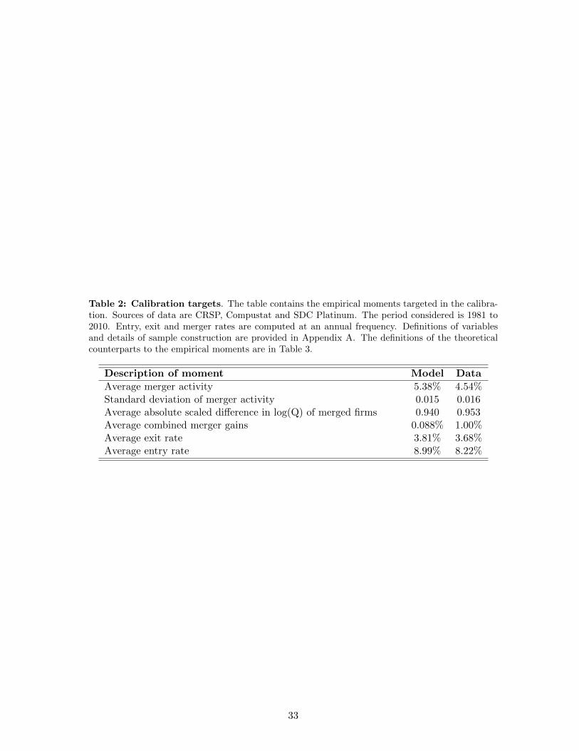
Table 2: Calibration targets. The table contains the empirical moments targeted in the calibra-tion. Sources of data are CRSP, Compustat and SDC Platinum. The period considered is 1981 to2010. Entry, exit and merger rates are computed at an annual frequency. Definitions of variablesand details of sample construction are provided in Appendix A. The definitions of the theoreticalcounterparts to the empirical moments are in Table 3.

Description of moment Model DataAverage merger activity 5.38% 4.54%Standard deviation of merger activity 0.015 0.016Average absolute scaled difference in log(Q) of merged firms 0.940 0.953Average combined merger gains 0.088% 1.00%Average exit rate 3.81% 3.68%Average entry rate 8.99% 8.22%

33

Table 3: Definition of simulated moments.

Tobin’s Q V (x,z,k)k

Combined merger gains for firm i and jW (x,zi,zj)

V (x,zi,ki)+V (x,zj ,kj)

Sales szkα

Operating income/Capitalszkα−cf

k

Investment rate k�−(1−δ)kk

34

Table 4: Correlations of simulated entry, exit and merger activity with aggregate shock.The probabilities are computed in the simulation step of the solution algorithm described in Ap-pendix B. Parameter values are shown in Table 1.

Description of moment ModelCorrelation of aggregate shock and entry 0.8965Correlation of aggregate shock and exit -0.9249Correlation of aggregate shock and merger activity 0.8908

35

Table 5: Regression coefficients of simulated probabilities of entry, exit and merger onstate variables. The probabilities are computed in the simulation step of the solution algorithmdescribed in Appendix B. Parameters are set to the values shown in Table 1 for the columnsdenoted as “With Mergers”, while µ is set to zero for the remaining two columns. s denotes theaggregate productivity shock, m and v are, respectively, the mean and variance of the cross-sectionaldistribution of firms’ idiosyncratic log productivity shocks, z. Standard errors of the OLS regressioncoefficients are reported in parentheses.

With Mergers Without MergersProb. of Merger Prob. of Entry Prob. of Exit Prob. of Entry Prob. of Exit

log(s) 0.4017 0.3367 -0.5748 0.3076 -1.1088(0.0202) (0.0185) (0.0274) (0.0176) (0.0395)

m -0.6446 0.0263 -0.436 0.1991 -0.8722(0.2000) (0.1836) (0.2716) (0.1532) (0.3449)

log(v) 0.0005 -0.0013 0.0695 0.0614 0.1736(0.0189) (0.0173) (0.0256) (0.0398) (0.0896)

Constant 0.1375 0.0131 0.347 0.2568 0.8084(0.0915) (0.084) (0.1242) (0.1531) (0.3447)

36

Table 6: Simulated moments for different sets of structural parameters. The startingparameter values are those in Table 1. Column (1) presents the base case of no exit, no entry andno mergers (cE → ∞, cf = 0, µ = 0). In Column (2) there is positive entry and exit, but mergersare not possible (µ = 0). Column (3) shows the simulated moments when mergers are allowed andall parameters are equal to those in Table 1. The following four columns present comparative staticsexercises: λ = 1 in Column (4); λ = 0 in Column (5); and θ = 0.1 in Column (6). The definitionsof the variables are in Table 3.

(1) (2) (3) (4) (5) (6)Sales

Mean 33.518 39.033 51.826 55.951 41.738 65.9093Standard deviation 18.358 19.914 30.785 34.964 23.297 46.5466

Operating income/CapitalMean 0.121 0.057 0.075 0.079 0.061 0.0848Standard deviation 0.019 0.039 0.041 0.042 0.040 0.0476

Investment rateMean 0.203 0.149 0.088 0.074 0.136 0.0504Standard deviation 0.356 0.332 0.320 0.319 0.331 0.3225

Idiosyncratic Productivity z

Mean 1.011 1.058 1.145 1.168 1.077 1.217Standard deviation 0.149 0.147 0.179 0.194 0.154 0.2363

Calibration targetsAvg. Entry Rate 0.078 0.090 0.085 0.084 0.0831Avg. Exit Rate 0.076 0.038 0.023 0.068 0.0000Avg. merger activity 0.054 0.068 0.010 0.0833St. Dev. merger activity 0.015 0.008 0.010 0.0059Avg. merger gains 0.009 0.016 0.006 0.0386Avg. log(Q) difference 0.940 1.288 0.362 1.048

37

Table 7: VAR coefficient estimates. This table presents the coefficient estimates of the vec-tor autoregression in Equation 11, which governs firms’ expectations about the law of motion ofaggregate states. The coefficients are computed using simulated data, as described in Appendix B.Parameters are set to the values shown in Table 1 for the columns denoted as “With Mergers”, whilethe matching rate µ is set to zero for the remaining two columns. s denotes the aggregate produc-tivity shock, and m and v are, respectively, the mean and variance of the cross-sectional distributionof firms’ idiosyncratic log productivity shocks, z. Standard errors are reported in parentheses.

With Mergers Without Mergersm

�log(v�) m

�log(v�)

m 0.1729 -2.0395 0.6177 0.1409(0.0848) (0.8294) (0.0901) (0.3721)

log(v) 0.0255 0.1739 0.0783 -0.0202(0.008) (0.0784) (0.0234) (0.0967)

log(s�) -0.0176 -0.099 0.0076 -0.0125(0.0092) (0.0900) (0.0108) (0.0445)

log(s) 0.1099 1.7921 -0.197 1.0246(0.0104) (0.1013) (0.0123) (0.051)

Constant 0.1971 -2.8268 0.3322 -4.0992(0.0388) (0.3800) (0.0900) (0.3717)

38

Table 8: Average and median absolute value of the difference between target andacquirer log(Tobin’s Q). The definition of Tobin’s Q is provided in Appendix A. Values arescaled by the standard deviation of log(Tobin’s Q) in the acquirer’s industry in the year of themerger transaction.

Year Observations Mean Median1981 57 0.8495 0.56991982 56 0.8976 0.86011983 54 1.0193 0.74911984 70 0.9601 0.74451985 67 1.1777 0.98491986 74 0.9970 0.76141987 71 1.1361 0.85971988 73 0.9715 0.73181989 67 1.1177 0.90001990 46 1.0737 0.75261991 46 0.8740 0.68261992 42 0.7762 0.55601993 43 0.9953 0.71001994 89 0.8486 0.66471995 114 0.8438 0.68881996 160 0.9134 0.70491997 173 0.8378 0.70781998 195 1.0109 0.83711999 221 0.9525 0.74202000 179 0.9576 0.79332001 143 1.0571 0.93432002 88 0.8844 0.71172003 82 0.9231 0.67252004 82 0.7956 0.65192005 91 0.8963 0.70092006 95 0.9499 0.71242007 112 0.9743 0.79912008 62 0.9741 0.72862009 40 1.1125 1.07502010 59 1.0204 0.6728All 2,751 0.9534 0.7498

39

Figure 1: Merger and exit activity in the sample of CRSP firms, 1926-2010. Shaded areas areperiods of economic recession (NBER).

8%

6%

4%

2%

0%

19601930 1940 1950 1970 1980 1990 2000 2010

% firms merged (CRSP) Recession

(a) Merger activity

0%

2%

4%

6%

8%

1930 1940 1950 1960 1970 1980 1990 2000 2010

% Firms exiting (CRSP) Recession

(b) Exit

40

Figure 2: Timing of events within each period for incumbents and potential entrants.

Incumbents

Observe beginning

of period states

(x, z, k)

Match with

merger partner

with probability µMerger

decision

Investment

decision

Period payoff

realized

Exit

decision

t t + 1

Potential entrants

Observe beginning

of period states

(x, y)Entry decision

pay cost cEInvestment

decision

t t + 1

41

Figure 3: Marginal productivity of the merged firm, zM , as a function of the productivities of thetwo matched firms, z1 and z2. In both figures, θ = 1

2 .

(a) λ = 1

(b) λ = 0

42

Figure 4: Merger synergies as a function of productivity shocks for the two matching firms, z1 andz2. Figure (a) shows the case for λ = 1, figure (b) shows the case of λ = 0. The white plane isthe locus of points for which merger synergies are zero. For the region of z1 and z2 where synergiesare positive, the matched firms merge. We set µ = 0.34, θ = 0.1, cM = 90, cE = 80, and cf = 20.The remaining parameter values are shown in Panel A of Table 1. States m and v are set at theiraverage levels in the simulation, and s = 1.

(a) λ = 1

(b) λ = 0

43

Figure 5: Entry and exit productivity thresholds (ζE , ζ�) as a function of the aggregate shock(s). Parameter values are shown in Table 1. States m and v are set at their average levels in thesimulation.

0.85 0.9 0.95 1 1.05 1.1 1.15

1.25

1.3

1.35

1.4

1.45

1.5

1.55

1.6

Aggregate state s

!E

(a) Entry threshold (ζE)

0.85 0.9 0.95 1 1.05 1.1 1.15-0.35

-0.3

-0.25

-0.2

-0.15

-0.1

-0.05

0

Aggregate shock s

!"

(b) Exit threshold (ζ�)

44

Figure 6: Merger synergies as a function of productivity shocks for the two matching firms, z1and z2. Figure (a) shows the case for s = 0.8871 (low aggregate productivity), figure (b) shows thecase of s = 1.1273 (high aggregate productivity). The white plane is the locus of points for whichmerger synergies are zero. For the region of z1 and z2 where synergies are positive, the matchingfirms merge. Parameter values are shown in Table 1. States m and v are set at their average levelsin the simulation.

(a) Low aggregate productivity

(b) High aggregate productivity

45

Figure 7: Simulated cross-sectional distribution of firms’ idiosyncratic productivity shocks, z.Figure (a) shows the distribution of z for incumbent firms and for new entrants in the industry, forthe case in which there are no mergers, µ = 0. Figure (b) shows the distribution of z for incumbentfirms, entrants, merging firms, and stand-alone firms – firms that were matched but decided not tomerge. Parameters are set to the values presented in Table 1. The distributions derive from pooling800 time-specific distributions obtained by non-stochastic simulation.

0.6 0.8 1 1.2 1.4 1.6 1.8 20

0.5

1

1.5

2

2.5

3

3.5

Idiosyncratic productivity shock z

EntrantsIncumbents

(a) Entry, exit, without mergers

0.6 0.8 1 1.2 1.4 1.6 1.8 20

0.5

1

1.5

2

2.5

3

3.5

4

Idiosyncratic productivity shock z

EntrantsIncumbentsMergedStand-alone

(b) Entry, exit, mergers

46

Figure 8: Impulse response functions for a positive shock to aggregate productivity (s). Parametersare set to the values shown in Table 1. Impulse responses are computed using the simulated data,as described in Appendix B.

0 10 20 30 40 500

0.5

1

1.5

2

2.5

3

3.5

Time

% D

evia

tion

(a) Aggregateshock

0 10 20 30 40 500

2

4

6

8

10

12

Time

% D

evi

atio

n

With MergersWithout Mergers

(b) Numberof firms

0 10 20 30 40 50-0.4

-0.3

-0.2

-0.1

0

0.1

0.2

0.3

0.4

Time

% D

evi

atio

n

With MergersWithout Mergers

(c) Average idiosyncraticproductivity shock z

0 10 20 30 40 50-2

-1.5

-1

-0.5

0

0.5

Time

% D

evi

atio

n

With Mergers

Without Mergers

(d) Entrants’ avg. id.productivity shock z

0 10 20 30 40 50-3

-2.5

-2

-1.5

-1

-0.5

0

0.05

Time

% D

evi

atio

n

With Mergers

Without Mergers

(e) Exitors’ avg. id.productivity shock z

0 10 20 30 40 500

2

4

6

8

10

12

14

Time

% D

evia

tion

(f) Merged firms’ avg. id.productivity shock z

0 10 20 30 40 500.275

0.28

0.285

0.29

0.295

0.3

0.305

0.31

0.315

Time

Log Idio

syncr

atic

Pro

duct

ivity

Shock

z

With Mergers

Without Mergers

(g) Entry threshold

0 10 20 30 40 50-0.18

-0.17

-0.16

-0.15

-0.14

-0.13

Time

Log Idio

syncr

atic

Pro

duct

ivity

Shock

z

With Mergers

WIthout Mergers

(h) Exit threshold

0 10 20 30 40 500

2

4

6

8

10

12

14

Time

% D

evia

tion

(i) Merger rate

47