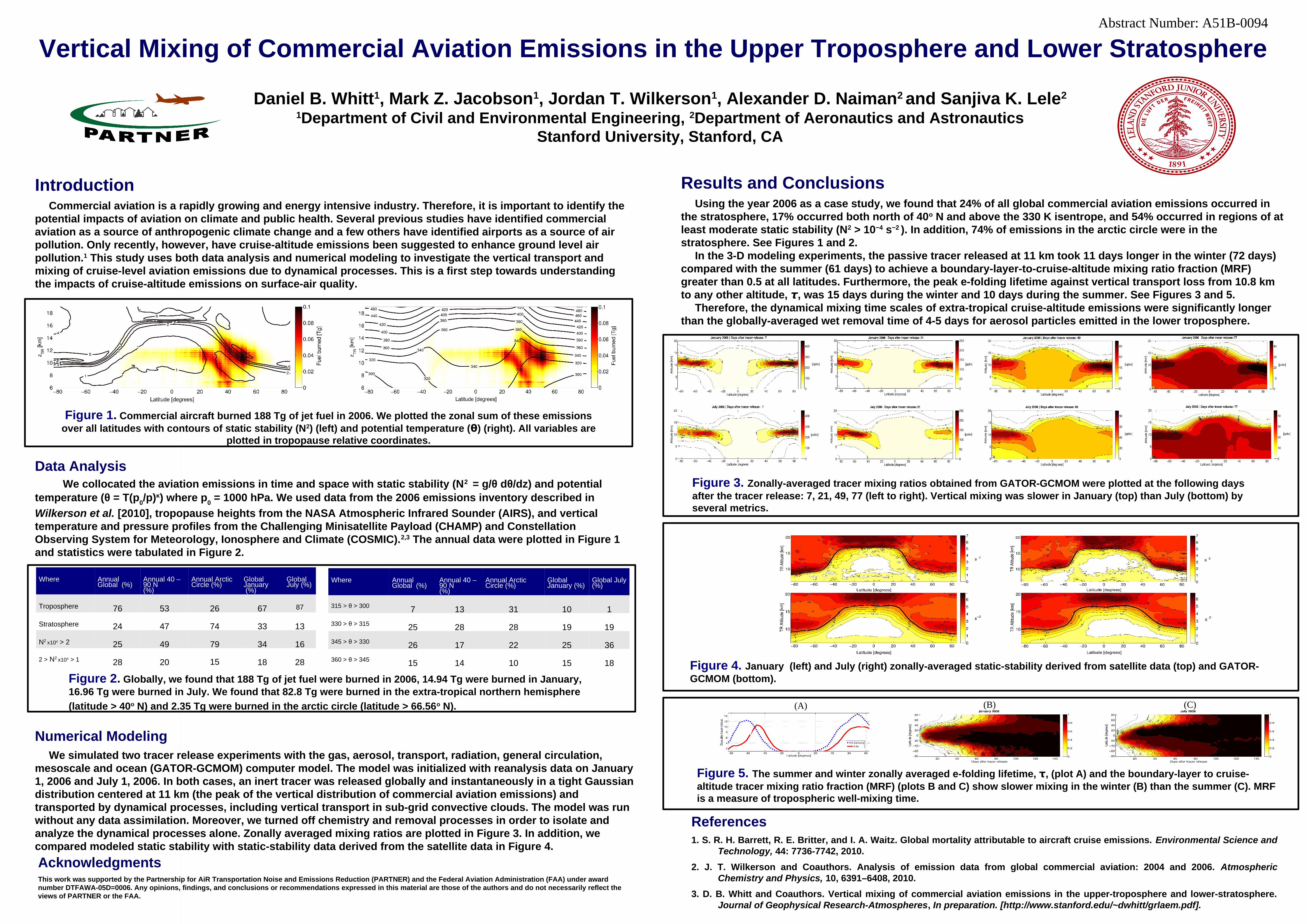
Vertical Mixing of Commercial Aviation Emissions in the Upper Troposphere and Lower Stratosphere

AcknowledgmentsThis work was supported by the Partnership for AiR Transportation Noise and Emissions Reduction (PARTNER) and the Federal Aviation Administration (FAA) under award number DTFAWA-05D=0006. Any opinions, findings, and conclusions or recommendations expressed in this material are those of the authors and do not necessarily reflect the views of PARTNER or the FAA.

Daniel B. Whitt1, Mark Z. Jacobson1, Jordan T. Wilkerson1, Alexander D. Naiman2 and Sanjiva K. Lele2

1Department of Civil and Environmental Engineering, 2Department of Aeronautics and AstronauticsStanford University, Stanford, CA

IntroductionCommercial aviation is a rapidly growing and energy intensive industry. Therefore, it is important to identify the

potential impacts of aviation on climate and public health. Several previous studies have identified commercial aviation as a source of anthropogenic climate change and a few others have identified airports as a source of air pollution. Only recently, however, have cruise-altitude emissions been suggested to enhance ground level air pollution.1 This study uses both data analysis and numerical modeling to investigate the vertical transport and mixing of cruise-level aviation emissions due to dynamical processes. This is a first step towards understanding the impacts of cruise-altitude emissions on surface-air quality.

Figure 1. Commercial aircraft burned 188 Tg of jet fuel in 2006. We plotted the zonal sum of these emissions over all latitudes with contours of static stability (N2) (left) and potential temperature (θ) (right). All variables are

plotted in tropopause relative coordinates.

References1. S. R. H. Barrett, R. E. Britter, and I. A. Waitz. Global mortality attributable to aircraft cruise emissions. Environmental Science and

Technology, 44: 7736-7742, 2010.

2. J. T. Wilkerson and Coauthors. Analysis of emission data from global commercial aviation: 2004 and 2006. Atmospheric Chemistry and Physics, 10, 6391–6408, 2010.

3. D. B. Whitt and Coauthors. Vertical mixing of commercial aviation emissions in the upper-troposphere and lower-stratosphere. Journal of Geophysical Research-Atmospheres, In preparation. [http://www.stanford.edu/~dwhitt/grlaem.pdf].

Data AnalysisWe collocated the aviation emissions in time and space with static stability (N2 = g/θ dθ/dz) and potential

temperature (θ = T(p0/p)κ) where p

0 = 1000 hPa. We used data from the 2006 emissions inventory described in

Wilkerson et al. [2010], tropopause heights from the NASA Atmospheric Infrared Sounder (AIRS), and vertical temperature and pressure profiles from the Challenging Minisatellite Payload (CHAMP) and Constellation Observing System for Meteorology, Ionosphere and Climate (COSMIC).2,3 The annual data were plotted in Figure 1 and statistics were tabulated in Figure 2.

Figure 2. Globally, we found that 188 Tg of jet fuel were burned in 2006, 14.94 Tg were burned in January, 16.96 Tg were burned in July. We found that 82.8 Tg were burned in the extra-tropical northern hemisphere

(latitude > 40o N) and 2.35 Tg were burned in the arctic circle (latitude > 66.56o N).

Results and ConclusionsUsing the year 2006 as a case study, we found that 24% of all global commercial aviation emissions occurred in

the stratosphere, 17% occurred both north of 40o N and above the 330 K isentrope, and 54% occurred in regions of at least moderate static stability (N2 > 10−4 s−2 ). In addition, 74% of emissions in the arctic circle were in the stratosphere. See Figures 1 and 2.

In the 3-D modeling experiments, the passive tracer released at 11 km took 11 days longer in the winter (72 days) compared with the summer (61 days) to achieve a boundary-layer-to-cruise-altitude mixing ratio fraction (MRF) greater than 0.5 at all latitudes. Furthermore, the peak e-folding lifetime against vertical transport loss from 10.8 km to any other altitude, τ, was 15 days during the winter and 10 days during the summer. See Figures 3 and 5.

Therefore, the dynamical mixing time scales of extra-tropical cruise-altitude emissions were significantly longer than the globally-averaged wet removal time of 4-5 days for aerosol particles emitted in the lower troposphere.

Figure 3. Zonally-averaged tracer mixing ratios obtained from GATOR-GCMOM were plotted at the following days after the tracer release: 7, 21, 49, 77 (left to right). Vertical mixing was slower in January (top) than July (bottom) by several metrics.

Abstract Number: A51B­0094

Where Annual Global (%)

Annual 40 – 90 N(%)

Annual Arctic Circle (%)

Global January (%)

Global July (%)

Troposphere 76 53 26 67 87

Stratosphere 24 47 74 33 13

N2 x104 > 2 25 49 79 34 16

2 > N2 x104 > 1 28 20 15 18 28

Where Annual Global (%)

Annual 40 – 90 N(%)

Annual Arctic Circle (%)

Global January (%)

Global July (%)

315 > θ > 300 7 13 31 10 1

330 > θ > 315 25 28 28 19 19

345 > θ > 330 26 17 22 25 36

360 > θ > 345 15 14 10 15 18

Figure 5. The summer and winter zonally averaged e-folding lifetime, τ, (plot A) and the boundary-layer to cruise-altitude tracer mixing ratio fraction (MRF) (plots B and C) show slower mixing in the winter (B) than the summer (C). MRF is a measure of tropospheric well-mixing time.

(A) (B) (C)

Numerical Modeling We simulated two tracer release experiments with the gas, aerosol, transport, radiation, general circulation,

mesoscale and ocean (GATOR-GCMOM) computer model. The model was initialized with reanalysis data on January 1, 2006 and July 1, 2006. In both cases, an inert tracer was released globally and instantaneously in a tight Gaussian distribution centered at 11 km (the peak of the vertical distribution of commercial aviation emissions) and transported by dynamical processes, including vertical transport in sub-grid convective clouds. The model was run without any data assimilation. Moreover, we turned off chemistry and removal processes in order to isolate and analyze the dynamical processes alone. Zonally averaged mixing ratios are plotted in Figure 3. In addition, we compared modeled static stability with static-stability data derived from the satellite data in Figure 4.

Figure 4. January (left) and July (right) zonally-averaged static-stability derived from satellite data (top) and GATOR-GCMOM (bottom).