Embed Size (px)
Citation preview

Abstract
Key words: 1l -NORM CONSTRAINT; LASSO; VARIABLE SELECTION; SUBSET SELECTION;
BAYSIAN LOGISTIC REGRESSION
LASSO is an innovative variable selection method for regression. Variable selection in regression is extremely important when we have available a large collection of possible covariates from which we hope to select a parsimonious set for the efficient prediction of a response variable. LASSO minimizes the residual sum of squares subject to the sum of the absolute value of the coefficients being less than a constant. LASSO not only helps to improve the prediction accuracy when dealing with multicolinearity data, but also carries several nice properties such as interpretability and numerical stability. This project also includes a couple of numerical approaches for solving LASSO. Case studies and simulations are studied in both the linear and logistic LASSO models, and are implemented in R; the source code is available in the appendix.

University of Minnesota Duluth
II
Acknowledgements
I would like to express my special thanks to my advisor, Dr. Kang James. She found this interesting topic for me and helped me to overcome the difficulties throughout this research. She taught me how to do research and what attitude and characteristics will lead me to success and happiness. She also helped me develop my presentation skills and was very encouraging. Thank Drs. Barry James and Yongcheng Qi for being my committee members and helping me with my thesis defense. I would like to thank my friend Lindsey Dietz and my boy friend Brad Jannsen for their help in proof reading my thesis. I would also like to acknowledge the support from my parents in China who always motivated me to work hard.

University of Minnesota Duluth
1
Table of Contents Acknowledgements ....................................................................................................... I Abstract......................................................................................................................... II Chapter 1 Introduction...................................................................................................2 Chapter 2 LASSO application in the Linear Regression Model ...................................4
2.1 The principle of the generalized linear LASSO model ....................................4 2.2 Geometrical Interpretation of LASSO..............................................................7 2.3 Prediction Error and Mean Square Error..........................................................8 2.4 CV/GCV methods and Estimate of LASSO parameter....................................9 2.5 Standard Error of LASSO Estimators.............................................................12 2.6 Case Study: Diabetes data ..............................................................................13 2.7 Simulation.......................................................................................................17
Chapter 3 LASSO application in the Logistic Regression Model............................. 21 3.1 Logistic LASSO model and Maximum likelihood estimate ..........................21 3.2 Maximum likelihood estimate and Maximum a posteriori estimate ..............24 3.3 Case study: Kyphosis data..............................................................................27 3.4 Simulation.......................................................................................................29
Chapter 4 Computation of LASSO..............................................................................31 4.1Osborne’s dual algorithm.................................................................................31 4.2 Least Angle Regression algorithm..................................................................32
References ...................................................................................................................34 Appendix .....................................................................................................................35

University of Minnesota Duluth
2
Chapter 1 Introduction A “lasso” is usually recognized as a loop of rope that is designed to be thrown around a target
and tighten when pulled. It is a well-known tool of the American cowboy. In this context, it is
fittingly being used as a metaphor of 1l constraint applied to linear model. Coincidently,
LASSO is also the initials for Least Absolute Shrinkage and Selection Operator.
Consider the usual linear regression model with data 1 2( , , , , ), 1, ,i i ip ix x x y i n= , where
the ijx ’s are the regressors and iy is the response variable of the i th observation. The
ordinary Least Squares (OLS) regression method finds the unbiased linear combination of
the ijx ’s that minimizes the residual sum of squares. However, if p is large or the regression
coefficients are highly correlated (multicolinearity), the OLS may yield estimates with large
variance which reduces the accuracy of the prediction. A widely-known method to solve this
problem is Ridge Regression and subset selection. As an alternative to these techniques,
Robert Tibshirani (1996) presented “LASSO” which minimized the residual sum of squares
subject to the sum of absolute values of the coefficient being less than a constant.
2
1
ˆ arg min{ ( ) }N
Li j ij
i jy xβ α β
=
= − −∑ ∑ (1.1)
subject to
1
ˆp
Lj
jtβ
=
≤∑ (Constant) . (1.2)
If 1
ˆp
oj
jt β
=
>∑ , then the LASSO algorithm will yield the same estimate as OLS estimate.
However, if 1
ˆ0p
oj
jt β
=
< <∑ , then the problem is equivalent to
2
1
ˆ arg min ( )N
Li j ij j
i j jy xβ α β λ β
=
⎛ ⎞= − − +⎜ ⎟
⎝ ⎠∑ ∑ ∑ , (1.3)
0λ > . It will be shown later that the relation between λ and LASSO parameter t is
one-to-one. Due to the nature of the constraint, LASSO tends to produce some coefficients to

University of Minnesota Duluth
3
be exactly zero. Compared to the OLS, whose predicted coefficient ˆ oβ is an unbiased
estimator ofβ , both ridge regression and LASSO sacrifice a little bias to reduce the variance
of the predicted values and improve the overall prediction accuracy.
In my project, I focus on two main aspects of this topic. In chapter 2, definitions and
principles of LASSO in both the generalized linear case and orthogonal case are discussed. In
Chapter 3, I illustrate the principles of the LASSO logistic model and give a couple of
examples. Chapter 4 introduces the existing algorithm for solving LASSO estimates. Finally,
I study two main numerical algorithms.

University of Minnesota Duluth
4
Chapter 2 Linear LASSO Model
2.1 The principle of the generalized linear LASSO model
Let2
1( , , , )
p
i j ij jj j
G X Y y xβ λ β λ β=
⎛ ⎞= − +⎜ ⎟
⎝ ⎠∑ ∑ ∑ ; G can also be written in matrix form
( , , , ) ( ) ( )TpG X Y Y X Y X Iβ λ β β λ β= − − + , (2.1.1)
Minimizing G, we can get best estimate ofβ which can be notated as β .
Let pI represent the p p× identity matrix, β be the diagonal matrix with j th diagonal
element jβ , X be the design matrix.
( )1
2
0 00
0
0 0
j
p
diag
ββ
β β
β
⎡ ⎤⎢ ⎥⎢ ⎥= =⎢ ⎥⎢ ⎥⎢ ⎥⎣ ⎦
, ( )
11
11 12
1
0 0
00
0 0
j
p
diag
β
ββ β
β
−
−− −
−
⎡ ⎤⎢ ⎥⎢ ⎥
= =⎢ ⎥⎢ ⎥⎢ ⎥⎢ ⎥⎣ ⎦
.
We will use these notations through out the rest of this paper.
Firstly, we note that (2.1.1) can be written as
( , , , ) T T T T T TG X Y Y Y X Y Y X X Xβ λ β β β β λ β= − − + + . (2.1.2)
Take partial derivative of (2.1.2) with respect toβ :
( , , , )2 2( ) ( )T TG X YY X X X sign
β λβ λ β
β∂
= − + +∂
, (2.1.3)
where1( )
( )( )p
signsign
sign
ββ
β
⎡ ⎤⎢ ⎥= ⎢ ⎥⎢ ⎥⎣ ⎦
.
Set ( , , , )
0G X Yβ λ
β∂
=∂
(2.1.4), and solve for β . For simplicity, we assume X is
orthonormal, TX X I= .
ˆ ojβ denotes the OLS estimate. For the multivariate case, 1ˆ ( )o T T TX X X Y X Yβ −= = .

University of Minnesota Duluth
5
By solving (2.1.4), we obtain the following result:
( )ˆ ˆ ˆ2
L o Lj j jsignλβ β β= − . (2.1.5)
Lemma2.1 If ( )2
y x sign yλ= − , then x and y share the same sign.
( ) ( )2 2
y x sign y x y sign yλ λ= − ⇔ = +
If y is positive, ( )2
y sign yλ+ must be positive, then x is positive. On the contrary, if y is
negative, then x is negative. Thus, x and y share the same sign. ■
According to Lemma 2.1 and (2.1.5), ( )ˆ Ljsign β = ( )ˆ o
jsign β . Then (2.1.5) becomes
( )ˆ ˆ ˆ2
L o oj j jsignλβ β β= −
ˆ ˆ 0
2ˆ ˆ 0
2
o oj j
o oj j
if
if
λβ β
λβ β
⎧ − ≥⎪⎪= ⎨⎪ + <⎪⎩
ˆ ˆ[ 0] [ 0]ˆ ˆ
2 2o oj j
o oj jI I
β β
λ λβ β≥ <
⎛ ⎞ ⎛ ⎞= − + −⎜ ⎟ ⎜ ⎟⎝ ⎠ ⎝ ⎠
. (2.1.6)
It follows that
( )ˆ ˆ ˆ 1, ,2
L o oj j jsign j pλβ β β
+⎛ ⎞= − =⎜ ⎟⎝ ⎠
. (2.1.7)
+ denotes the positive part of expression inside the parenthesis.

University of Minnesota Duluth
6
Fig 2.1 Form of coefficient shrinkage of LASSO in the orthonormal case. LASSO. LASSO tends to
produce zero coefficients.
Intuitively, 2λ is the threshold set for nonzero estimates; in another words, if the
corresponding ˆ ojβ is less than the threshold, we will set ˆ L
jβ equal to zero.
The parameter λ can be computed by solving the equations
( )ˆ ˆ ˆ , (2.1.8)2
ˆ . (2.1.9)
L o oj j j
Lj
j
sign
t
λβ β β
β
+⎧ ⎛ ⎞= −⎪ ⎜ ⎟⎪ ⎝ ⎠⎨⎪ =⎪⎩∑
whereλ is chosen so that jj
tβ =∑ . Therefore, each λ value corresponds to a unique t
value. This is illustrated by solving the simplest case of p=2. Without loss of generality, we
assume that the least squares estimates ˆ ojβ are both positive.
1 1
2 2
ˆ ˆ2
ˆ ˆ2
L o
L o
λβ β
λβ β
+
+
⎧ ⎛ ⎞= −⎪ ⎜ ⎟⎪ ⎝ ⎠⎨
⎛ ⎞⎪ = −⎜ ⎟⎪ ⎝ ⎠⎩
(2.1.10) and 1 2ˆ ˆL L tβ β+ = . (2.1.11)
First solving for λ , I get
1 2ˆ ˆo o tλ β β= + − . (2.1.12)

University of Minnesota Duluth
7
Substituting (2.1.12) into (2.1.10), I obtain the solution for LASSO estimates
1 2 1 21 1
1 2 1 22 2
ˆ ˆ ˆ ˆˆ ˆ ,2 2 2
ˆ ˆ ˆ ˆˆ ˆ .2 2 2
o o o oL o
o o o oL o
t t
t t
β β β ββ β
β β β ββ β
+ +
+ +
⎧ ⎛ ⎞ ⎛ ⎞+ − −⎪ = − = +⎜ ⎟ ⎜ ⎟⎜ ⎟ ⎜ ⎟⎪⎪ ⎝ ⎠ ⎝ ⎠⎨
⎛ ⎞ ⎛ ⎞⎪ + − −= − = −⎜ ⎟ ⎜ ⎟⎪ ⎜ ⎟ ⎜ ⎟⎪ ⎝ ⎠ ⎝ ⎠⎩
(2.1.13)
When extended to the general case,
1
ˆ ˆ( )2
po oj j
i
t sign p λβ β=
= −∑ . (2.1.14)
Now it can be seen that the relationship between λ and the LASSO parameter t is
one-to-one. Unfortunately, LASSO estimate doesn’t usually have a closed-form solution.
However, statisticians have already developed several numerical approximation algorithms,
which will be discussed in Chapter 4.
2.2 Geometrical Interpretation of LASSO
Fig 2.2.1 A geometrical interpretation of LASSO in 2-dimension and 3-dimension. The left panel is from
Tibshirani (1996). The right panel is from Meinshausen (2008).
Fig 2.2.1 illustrates the geometric image of LASSO regression for the two- and three-
dimensional cases. Looking at the left panel, the center point of the ellipse is ˆ oβ (OLS
estimates). The ellipse contour corresponds to some specific residual sum of square values.

University of Minnesota Duluth
8
The area inside the square around the origin satisfies the LASSO restriction. It means that
1( ,..., )Tpβ β β= inside the black square satisfies the constraint j
j
tβ ≤∑ . This implies that
minimizing the residual sum of squares according to the constraint corresponds to the contour
tangent to the pyramid. The LASSO solution is the first place that the contours touch the
square; this will sometimes occur at a corner (due to the nature of the pyramid),
corresponding to a zero coefficient. It is the same in three dimensions. From the right panel
of Fig 2.2.1, one can see the contour touching one margin of the pyramid on the X-Y plane
which corresponds to 1 2,β β , so it assigns the value zero to the variable 3β .
2.3 Prediction Error and Mean Square Error
Suppose that ˆˆ( ) , ( )Y x x Xη ε η β= + = is an estimate of ( )x Xη β= , ε is random error with
normal distribution, and ( ) 20, ( )E Varε ε σ= = .
The mean-squared error of an estimate ˆ( )xη is defined by
2ˆ[ ( ) ( )]MSE E x xη η= − . (2.3.1)
It is hard to estimate MSE because ( )x Xη β= is unknown. However, predicted error is
easier to calculate and is closely related to MSE.
2ˆ[ ( )]PSE E Y xη= − 2MSE σ= + . (2.3.2)
Lemma 2.3 2PSE MSE σ= +
2 2ˆ ˆ[ ( )] [ ( ) ( ) ( )]PSE E Y x E Y x x xη η η η= − = − + −
2 2ˆ ˆ[ ( ) ( )] 2 [( ( ) ( ))( ( ))] [ ( )]E x x E x x Y x E Y xη η η η η η= − + − − + − .
The first and the third term 2 2[ ( )]E Y xη σ− = , 2ˆ[ ( ) ( )]E x x MSEη η− = , the middle term

University of Minnesota Duluth
9
[ ] ( )ˆ ˆ( ( ) ( ))( ( )) ( ) ( ) 0E x x Y x E x xη η η η η ε− − = − =⎡ ⎤⎣ ⎦ .
Thus, 2PSE MSE σ= + . Minimizing PSE is equivalent to minimizing MSE. In the next
section, I will introduce how to get the optimal LASSO parameter by minimizing the effect of
predicted error.
2.4 CV/GCV methods and Estimate of the LASSO parameter
2.4.1 Relative Bound and Absolute Bound
The tuning parameter t is called LASSO parameter, which is also recognized as the
absolute bound. 1
ˆn
Lj
j
tβ=
=∑ . Here I define another parameter, s , as the relative bound.
1
1
ˆ
. [0,1]ˆ
pL
jjp
oj
j
s sβ
β
=
=
= ∈∑
∑ (2.4.1)
The relative bound can be seen as a normalized version of LASSO parameter. There are two
algorithms mentioned in Tibshirani (1996) to compute the best s : N-fold Cross-validation
and Generalized Cross-validation(GCV).
2.4.2 N-fold Cross-validation
Cross-validation is a general procedure that can be applied to estimate tuning parameters in
a wide variety of problems. The bias in RSS is a result of using the same data for model
fitting and model evaluation. CV can reduce the bias of RSS by splitting the whole data into
two subsamples: a training (calibration) sample for model fitting and a test (validation)
sample for model evaluation. The idea behind the cross-validation is to recycle data by
switching the roles of training and test samples.

University of Minnesota Duluth
10
The optimal s can be denoted by s . Prediction error can be estimated for the LASSO
procedure by ten-fold cross-validation. The LASSO is indexed in terms of s , and the
prediction error is estimated over a grid of values of s from 0 to 1 inclusive. We wish to
predict with small variance, thus we wish to choose the constraint s as small as we can. The
value s which achieves the minimum predicted error of ˆ( )xη is selected (Tibshirani
1996).
For example, we have Acetylene data, which is from Marquardt, et al. 1975. In this data, the
corresponding variable y is percentage of conversion of n-Heptane to acetylene. The three
explanatory variables are:
T=Reactor Temperature (°C);
H=Ratio of H2 to n-Heptane (mole ratio);
C=Contact time (sec).
T and C are highly correlated variables the covariance matrix is
Accordingly, we will get very large variance for each estimates. Instead, if we use LASSO
method, we will get the following GCV score plot, we choose ˆ 0.25s = .
Fig 2.4.1 Acetylene data GCV versus s plot. (We will illustrate GCV in the next section)
T H CT 1 0.223628 -0.9582H 0.223628 1 -0.24023C -0.9582 -0.24023 1
University of Minnesota Duluth
11
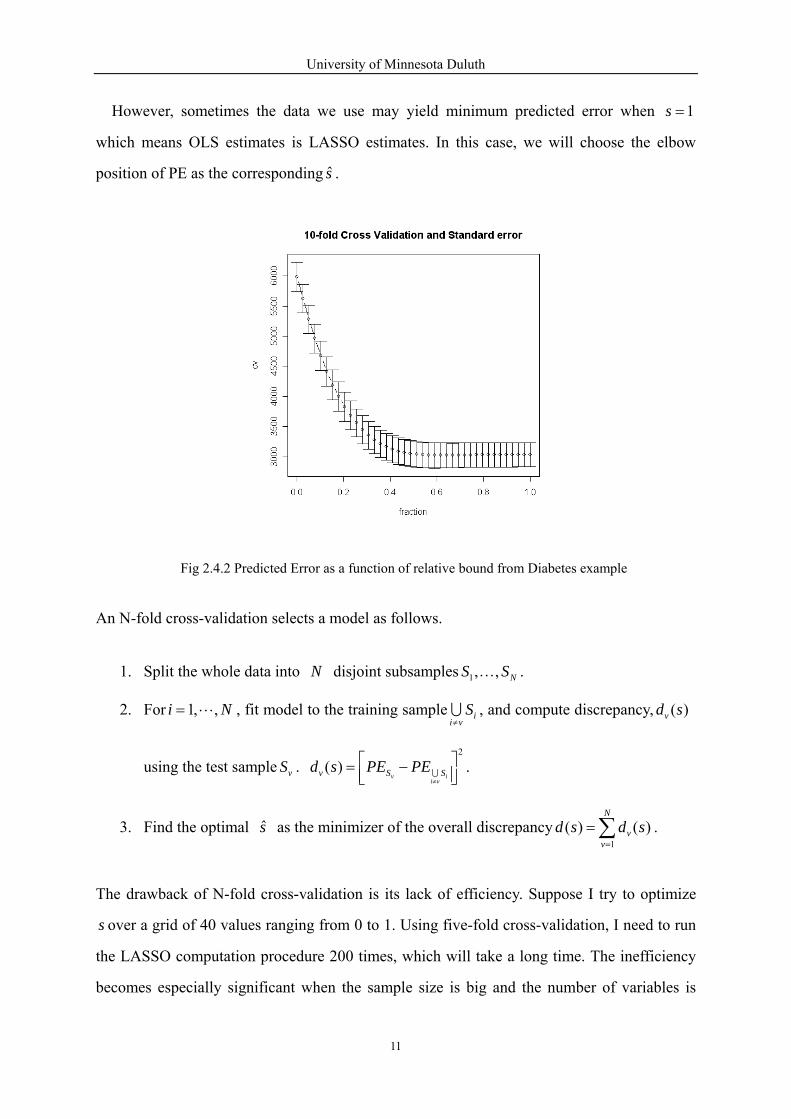
However, sometimes the data we use may yield minimum predicted error when 1s =
which means OLS estimates is LASSO estimates. In this case, we will choose the elbow
position of PE as the corresponding s .
Fig 2.4.2 Predicted Error as a function of relative bound from Diabetes example
An N-fold cross-validation selects a model as follows.
1. Split the whole data into N disjoint subsamples 1, , NS S… .
2. For 1, ,i N= , fit model to the training sample ii v
S≠∪ , and compute discrepancy, ( )vd s
using the test sample vS . 2
( )v i
i vv S Sd s PE PE
≠
⎡ ⎤= −⎢ ⎥⎣ ⎦∪ .
3. Find the optimal s as the minimizer of the overall discrepancy1
( ) ( )N
vv
d s d s=
= ∑ .
The drawback of N-fold cross-validation is its lack of efficiency. Suppose I try to optimize
s over a grid of 40 values ranging from 0 to 1. Using five-fold cross-validation, I need to run
the LASSO computation procedure 200 times, which will take a long time. The inefficiency
becomes especially significant when the sample size is big and the number of variables is

University of Minnesota Duluth
12
large. Due to this feature, Tibshirani (1996) introduced another algorithm: Generalized
Cross-validation(GCV) which has a significant computational advantage over N-fold
cross-validation.
2.4.3 Generalized Cross-validation
The generalized cross-validation (GCV) criterion was firstly proposed by Craven, P. and Wahba, G. (1979).
We have already proved in the previous section that
( )ˆ ˆ ˆ 1, ,2
L o oj j jsign j pλβ β β
+⎛ ⎞= − =⎜ ⎟⎝ ⎠
. (2.1.7)
If we rewrite it in matrix form,
11ˆ
2L T TX X X Yλβ β
−−⎛ ⎞= −⎜ ⎟
⎝ ⎠i . (2.4.2)
Therefore the effective number of parameters (Appendix A) in the model is
11
( )2
T Td Tr X X X Xλλ β−
−⎡ ⎤⎛ ⎞= −⎢ ⎥⎜ ⎟⎝ ⎠⎢ ⎥⎣ ⎦
i . (2.4.3)
We construct the generalized cross-validation statistic for LASSO to be
( )( )
2
12
ˆ1( )
1 /
nL
i ii
y xGCV
n d n
βλ
λ=
−=
−⎡ ⎤⎣ ⎦
∑. (2.4.4)
Compared to N-fold Cross-validation, GCV is more efficient. Suppose I still try to evaluate
s over a grid of 40 values ranging from 0 to 1. Using GCV instead, the LASSO computation
procedure only needs to run 40 times. However, there is also a drawback of GCV. A major
difficulty lies in the evaluation of the cross-validation function, which requires the calculation
of the trace of an inverse matrix. The problem becomes especially considerable when dealing

University of Minnesota Duluth
13
with large scale data. However, this is another area of study which will not be discussed here.
2.5 Standard Error of LASSO Estimators
LASSO estimate (2.1.5) can also be written as ( )ˆ ˆ ˆ2
L ojsignλβ β β= − ,
11ˆ
ˆ ˆˆ2 2
oL o T T
oX X X Y
βλ λβ β ββ
−−⎛ ⎞= − = −⎜ ⎟
⎝ ⎠i i . (2.5.1)
( )1
1ˆ2
L T TVar Var X X X Yλβ β−
−⎡ ⎤⎛ ⎞= −⎢ ⎥⎜ ⎟⎝ ⎠⎢ ⎥⎣ ⎦
i
1 1
1 1( )
2 2
T
T T T TX X X Var Y X X Xλ λβ β− −
− −⎛ ⎞⎛ ⎞ ⎛ ⎞= − −⎜ ⎟⎜ ⎟ ⎜ ⎟⎜ ⎟⎝ ⎠ ⎝ ⎠⎝ ⎠i i
1 1
1 12
2 2T T TX X X X X Xλ λσ β β
− −− −⎛ ⎞ ⎛ ⎞= − −⎜ ⎟ ⎜ ⎟
⎝ ⎠ ⎝ ⎠i i . (2.5.2)
2( )Var Y σ= is an estimate of the error variance. In my research, I usually use the bootstrap
(keep resampling from the original data set with replacement) method to estimate the
standard error of LASSO estimates.
2.6 Case Study: Diabetes data This data was originally used by Efron, Hastie, Johnstone and Tibshirani (2003). Table 2.6.1
shows a small portion of the data. There are ten baseline variables, age, sex, body mass index
(bmi), average blood pressure (BP) and six blood serum measurements. N=422 diabetes
patients were measured. The response variable y is a quantitative measure of disease
progression one year after baseline.
Obs AGE SEX BMI BP S1 S2 S3 S4 S5 S6 Y 1 59 2 32.1 101 157 93.2 38 4 4.8598 87 151

University of Minnesota Duluth
14
2 48 1 21.6 87 183 103.2 70 3 3.8918 69 75 3 72 2 30.5 93 156 93.6 41 4 4.6728 85 141 4 24 1 25.3 84 198 131.4 40 5 4.8903 89 206 5 50 1 23 101 192 125.4 52 4 4.2905 80 135 6 23 1 22.6 89 139 64.8 61 2 4.1897 68 97 … … … … … … … … … … … ... 438 60 2 28.2 112 185 113.8 42 4 4.9836 93 178 439 47 2 24.9 75 225 166 42 5 4.4427 102 104 440 60 2 24.9 99.67 162 106.6 43 3.77 4.1271 95 132 441 36 1 30 95 201 125.2 42 4.79 5.1299 85 220 442 36 1 19.6 71 250 133.2 97 3 4.5951 92 57
Table 2.6.1 Data structure of Diabetes Data
Ideally, the model would produce accurate baseline predictions of response for future patients,
and also the form of the model would suggest which covariates were important factors in
diabetes treatment progression.
Firstly, I evaluate the LASSO model on a grid of 40 s values. The optimal LASSO
parameter s by GCV scores can be observed. (see Fig 2.6.1)
Fig 2.6.1 GCV score as a function of relative bound s. ˆ 0.4s =
From Fig 2.6.1, one can see that the speed of GCV scores decreases dramatically until s =0.4.
Thus I pick 0.4 as our optimized s value.

University of Minnesota Duluth
15
In order to see how LASSO shrinks and predicts the coefficients more clearly, the LASSO
estimates as a function of the standardized relative bound s as plotted. Intuitively, every
coefficient will be squeezed to zero as s goes to zero.
1: age; 2: Sex; 3: BMI; 4: BP; 5~10: 6 levels of blood serum measurements
Fig 2.6.2: LASSO coefficient shrinkage in diabetes example: each monotone decreasing curve represents a coefficient as a function of relative bound s . The vertical lines show at which s value that each coefficient shrinks to zero. The covariates enter the regression equation sequentially as s increase, in order i=3,9,4,7,2,10,5,8,6,1. If s=0.4 as chosen by GCV, 9(S5) 3(BMI), as shown by the vertical red line, only the coefficients on the left of the red lines 4(BP) and 7(S3), and 2(Sex) are assigned to be nonzero.
Second, I evaluate Diabetes data at ˆ 0.4s = . The table below shows the LASSO estimate and
OLS g. The standard errors (SE) were estimated by bootstrap resampling of residuals from
the original data set. LASSO chooses sex, bmi, BP, S3 and S5. Notice that LASSO yielded
smaller SE for sex, bmi, BP, S3and S5 than those yielded by OLS. This shows that LASSO
predicts the coefficients with more accuracy. The table shows a tendency that LASSO
estimate is smaller than the ones by OLS. This is due to its constraint nature, that all
predictions are subtracted by a threshold value. Also, Cp statistics of OLS is 11 while Cp
statistics of LASSO is 5. Cp results illustrates that LASSO also has some good properties of
subset selection.

University of Minnesota Duluth
16
Predictor LASSO Results OLS Results Coefficients SE Z-score Pr(>|t|) Coefficients SE Z-score Pr(>|t|) Intercept 2.6461 0.30737 8.608846 0 152.133 2.576 59.061 < 2e-16 ***age 0 51.6555 0 1 -10.012 59.749 -0.168 0.867 sex -52.5341 56.18816 -0.93497 0.174903 -239.819 61.222 -3.917 0.000104 ***bmi 509.6485 57.26192 8.900304 0 519.84 66.534 7.813 4.30E-14 ***BP 221.3422 55.14417 4.013882 0.00003 324.39 65.422 4.958 1.02E-06 ***S1 0 106.5671 0 1 -792.184 416.684 -1.901 0.057947 . S2 0 89.25398 0 1 476.746 339.035 1.406 0.160389 S3 -153.097 69.5406 -2.20155 0.013848 101.045 212.533 0.475 0.634721 S4 0 77.67842 0 1 177.064 161.476 1.097 0.273456 S5 447.3803 73.6392 6.075301 0 751.279 171.902 4.37 1.56E-05 ***S6 0 45.80782 0 1 67.625 65.984 1.025 0.305998
Significant code: P-value “***” 0, “**” 0.001, “*” 0.01, “.” 0.05; Table 2.6.2 Results from Diabetes Data Example
2.7 Simulation Study
2.7.1 Autoregressive model
We use AR (1) model to generate multi-correlated variables.
AR (1) model is 0 1 1t t tx xφ φ ε−= + + , where 1 2,ε ε … is an i.i.d. sequence with mean 0 and
variance 2σ . Assuming weakly stationary, it is easy to see
0 1 1( ) ( )t tE x E xφ φ −= + . Substituted ( )tE x by μ , 0 1μ φ φ μ= + , then we can get
0
11φμφ
=−
. (2.7.1)
The variance can be inducted as following
( )1 1 11t t tx xφ μ φ ε−= − + + 1 1( )t t tx xμ φ μ ε−⇔ − = − +
( ) ( )( )1 1( , ) ( ) ( )l t t l t t l t t t lCov x x E x x E x xρ μ μ φ μ ε μ− − − −= = − − = − + −⎡ ⎤⎣ ⎦

University of Minnesota Duluth
17
( )( ) [ ] ( )( )1 1 1 1 1 1 1 1 0( ) lt t l t t t t l lE x x E x E x x r rφ μ μ ε μ φ μ μ φ φ− − − − − −= − − + − = − − = =⎡ ⎤ ⎡ ⎤⎣ ⎦ ⎣ ⎦ .
Since ijρ denotes the correlation between ix and jx ,. Simplifying, I can write 1φ φ= , which
will leads to
,ll
i i lo
rr
ρ φ− = = (2.7.2)
Given Signal-to-Noise ratio( SNR), which is defined asT XSNR βσ
= . In order to find φ , I
assume that 0xφ = (initial value of the sequence). Then we can easily calculate φ and 0x .
The details of calculation will be shown in the next section.
2.7.2 Simulation I
The model is Ty Xβ ε= + .
I generated 1000 observations with 8 correlated variables. The parameters are designed to be
(3,1.5,0,0,2,0,0,0)Tβ = . ε is random error with normal distribution ( )20,N σ . The
correlation between ix , jx was i jφ − , 0.5φ = , 3σ = . The data generated yields a SNR to be
approximately 5.7.
In our example, 0.5φ = l i j= − , i jij lρ ρ φ −= = .
According to ( )1 1 11 ( 1)t t tx xφ μ φ ε−= − + − + , we have 1 00.5 0.5 tx x μ ε= + + ;
( )2 1 0 00.5 0.5 0.5 0.5 0.5 0.5 0.75 0.25t t tx x x xμ ε μ μ ε μ ε= + + = + + + = + + ;
…

University of Minnesota Duluth
18
5 00.0625 0.9375x x μ= + ;
…
If I wish to get SNR=5.7 and 3σ = , then 5.7 3 17T Xβ = × = ,
Note that
( ) ( ) ( )1 2 5 0 0 03 1.5 3 3 0.5 0.5 1.5 0.75 0.25 2 0.0625 0.9375T X x x x x x xβ μ μ μ= + + = + + + + +
where 0x is a initial value, which can be set to be μ . Solving forμ , 0 2.6153xμ = = .
To generalize the procedure, 1
p
jj
SNR σ β μ=
⎛ ⎞× = ×⎜ ⎟
⎝ ⎠∑ , and 0
1
p
jj
SNRx σμβ
=
×= =
⎛ ⎞⎜ ⎟⎝ ⎠∑
. (2.7.3)
All initial values and means of the other simulation examples are decided by the same
method. The other two simulations followed the same procedure. The result of simulation I is
shown in Fig 2.7.1.
Fig 2.7.1 LASSO coefficient shrinkage in simulation 1: each monotone decreasing curve represents a coefficient as a function of relative bound s. The covariates enter the regression equation sequentially as s increase, in order i=1, 5, 2, 6, …, 7. If s=0.6, shown by the vertical red line, chosen by GCV (shown in
the right panel), variables 1, 5, 2 are nonzero, which is consistent with (3,1.5,0,0,2,0,0,0)Tβ = .

University of Minnesota Duluth
19
2.7.3 Simulation II
I generated 1000 observations with 8 correlated variables. The parameters are designed to
be (0.85,0.85,0.85,0.85,0.85,0.85,0.85,0.85)Tβ = . The correlation between ix ,
jx remains i jφ − , 0.5φ = , standard deviation of error is 3σ = . The data generated yields a
signal-to-noise ratio (SNR) of approximately 1.8. The result of Simulation II is shown in Fig
2.7.2.
Fig2.7.2 LASSO coefficient shrinkage in simulation 2: The GCV score plot doesn’t have an obvious elbow position. If I have to choose one, optimal s can be 0.8. The covariates enter the regression equation sequentially as s increase, in order i=5, 7, 3…, 8. If s=0.8, shown by the vertical red line, all variables are nonzero, which is consistent with the assigned (0.85,0.85,0.85,0.85,0.85,0.85,0.85,0.85)Tβ =
2.7.4 Simulation III
I generated 1000 observations with 8 correlated variables. The parameters are designed to
be (6,0,0,0,0,0,0,0)Tβ = . The correlation between ix , jx is still i jφ − , 0.5φ = , standard
deviation of error is 2σ = . The data generated yields a signal-to-noise ratio (SNR) of
approximately 7. The result of Simulation III is shown in Fig 2.7.3.

University of Minnesota Duluth
20
Fig 2.7.3 LASSO coefficient shrinkage in simulation 3: The GCV score plot one the right panel have an obvious elbow position, optimal s is approximately 0.6. The covariates enter the regression equation sequentially as s increase, the 1st variable enter first, all the other variables are hard to tell the order of entering. If s=0.6, only the 1st variable are nonzero, which is consistent with the assigned
(6,0,0,0,0,0,0,0)Tβ =
From Fig 2.7.3, because one of the variables is clearly more significant than the others, the
GCV score plot shows a more obvious elbow position. To generalize, the significance level
of variables determines how distinguished the elbow position is.

University of Minnesota Duluth
21
Chapter 3 Logistic LASSO model
3.1 Logistic LASSO model and Maximum likelihood estimate
3.1.1 Logistic LASSO model
The 1l -norm constraint of the LASSO can also be applied to logistic regression models
(Genkin et al., 2004) by minimizing the corresponding negative log-likelihood instead of the residual sum of squares. LASSO logistic model is similar to the LASSO linear model except
iY ’s can only take two possible values, 0 and 1. I will assume that the response variable iY is
a Bernoulli random variable with probability
( 1| , )i i iP Y x β π= = , ( 0 | , ) 1i i iP Y x β π= = − . (3.1.1)
It is easily proven that
( )i iE Y π= (3.1.2)
and ( )2 1iY i iσ π π= − . (3.1.3)
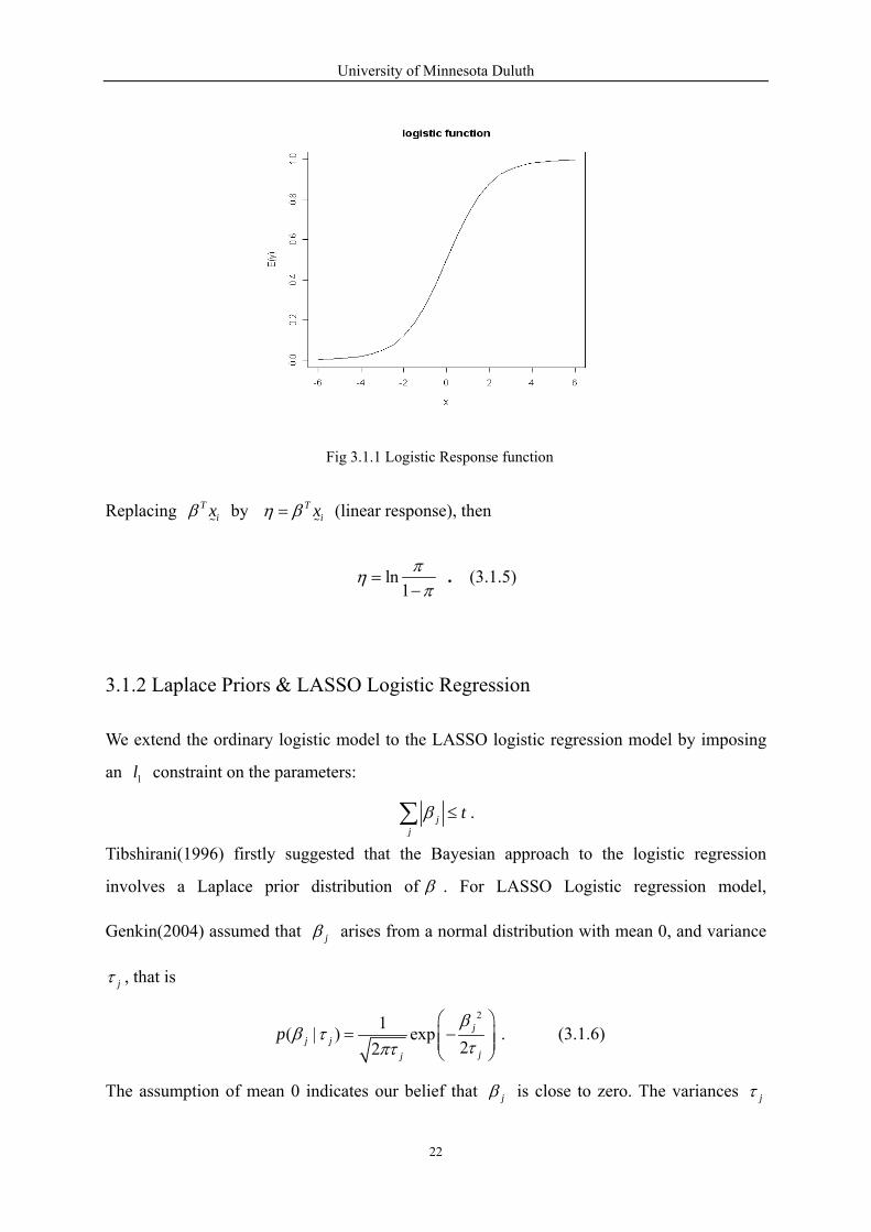
Generally, when the response variable is binary, a monotonically increasing (or decreasing) S-shaped function is usually employed. The function is called the logistic response function, or logistic function.
1( 1| , ) ( )1 exp( )i i i i
i
P Y x E Yx
ββ
= = =+ −
, (3.1.4)
University of Minnesota Duluth
22
Fig 3.1.1 Logistic Response function
Replacing Tixβ by T
ixη β= (linear response), then
ln1πηπ
=−
. (3.1.5)
3.1.2 Laplace Priors & LASSO Logistic Regression
We extend the ordinary logistic model to the LASSO logistic regression model by imposing
an 1l constraint on the parameters:
jj
tβ ≤∑ .
Tibshirani(1996) firstly suggested that the Bayesian approach to the logistic regression
involves a Laplace prior distribution of β . For LASSO Logistic regression model,
Genkin(2004) assumed that jβ arises from a normal distribution with mean 0, and variance
jτ , that is
21( | ) exp22
jj j
jj
pβ
β ττπτ
⎛ ⎞= −⎜ ⎟⎜ ⎟
⎝ ⎠. (3.1.6)
The assumption of mean 0 indicates our belief that jβ is close to zero. The variances jτ

University of Minnesota Duluth
23
are positive constants. A small value of jτ represents a prior belief that jβ is close to zero.
Conversely, a large value of jτ represents a less informative prior belief. In the simplest
case, assume that jτ τ= , for all j , and the component of β are independent and hence the
overall prior of β is the product of the prior of each of the components jβ ’s. Tibshirani
(1996) suggested jτ arises from an Laplace prior (double exponential distribution) with
density
( )| exp2 2
j jj j jp
γ γτ γ τ
⎛ ⎞= −⎜ ⎟
⎝ ⎠. (3.1.7)
Integrating out jτ can give us the distribution of jβ as follows (Lemma 3.1)
( )| exp2 2
j jj j jp
ζ ζβ ζ β
⎛ ⎞= −⎜ ⎟
⎝ ⎠, j jζ γ= . (3.1.8)
Lemma 3.1 β arises from a normal distribution with mean 0, and varianceτ , andτ arises
from an Laplace prior with coefficientγ , then ( )| exp2 2
pγ γ
β γ β⎛ ⎞
= −⎜ ⎟⎜ ⎟⎝ ⎠
. .
( )0
| ( | ) ( | )p p p dβ γ β τ τ γ τ∞
= ∫
2
0
1 1 exp2 2 22
dγ γ βτ ττπ π
∞ ⎡ ⎤⎛ ⎞= − +⎢ ⎥⎜ ⎟
⎝ ⎠⎣ ⎦∫ .
Substituting2
x γ τ= , 2 2d dxττγ
= and2 2
22 4xβ β γτ= leads to
( )2
220
| exp4
p x dxx
γ β γβ γπ
∞ ⎡ ⎤⎛ ⎞= − +⎢ ⎥⎜ ⎟
⎝ ⎠⎣ ⎦∫ .
We know that [ ]2
220
exp exp 22
a x dx ax
π∞ ⎡ ⎤⎛ ⎞− + = −⎢ ⎥⎜ ⎟⎝ ⎠⎣ ⎦
∫ , where2
a β γ= . Now we reach our
designated form ( )| exp2 2
pγ γ
β γ β⎛ ⎞
= −⎜ ⎟⎜ ⎟⎝ ⎠
. If we do substitutionζ γ= , we have

University of Minnesota Duluth
24
( )| exp2 2
p ζ ζβ ζ β⎛ ⎞= −⎜ ⎟⎝ ⎠
■ This is the density of double exponential distribution. Fig 3.1.2 gives the plot of this density function together with normal density function.
Fig 3.1.2 Double exponential density function (black) and normal density function (red).
From the Fig 3.1.2, I can see that Laplace prior (double exponential distribution) favor values
around 0, which indicates that LASSO favors zeros as estimates for some variables.
3.2 Maximum likelihood and Maximum a Posteriori estimate
3.2.1 Maximum Likelihood (ML) Estimate
Firstly recall the linear logistic regression model; we will use maximum likelihood to
estimate the parameters in Tixβ . The density function of each sample observation is
1( ) (1 )i iy yi i i if y π π −= − . (3.2.1)
Since each observation is assumed to be independent, the likelihood function is
1
1 1
( , ) ( ) (1 )i i
n ny y
i i i ii i
L Y f yβ π π −
= =
= = −∏ ∏ . (3.2.2)
The log-likelihood function is
( )1 1 1 11
ln ( , ) ln ( ) ln ln 1 ln 1 exp( )1
n n n n nT Ti
i i i i i i ii i i ii i
L Y f y y y x xπβ π β βπ= = = ==
⎡ ⎤⎛ ⎞⎡ ⎤= = + − = − +⎢ ⎥⎜ ⎟ ⎣ ⎦−⎝ ⎠⎣ ⎦
∑ ∑ ∑ ∑∏ .

University of Minnesota Duluth
25
Let ( )( )
expln ( , ) 01 exp
TiT T
i i iTi i i
xd L Y y x xd x
βββ β
⎡ ⎤⎢ ⎥= − =+⎢ ⎥⎣ ⎦
∑ ∑ . (3.2.4)
We can solve (3.2.4) and get an estimate forβ
There is no closed-form solution for this likelihood equation. The most common optimization
approach in statistical software, such as SAS and Splus/R , is multidimensional Newton-
Raphson algorithm implemented via iteratively reweighted least squares (IRLS) algorithm
(Dennis and Schnabel 1989; Hastie and Pregibon 1992). Newton-Raphson method has the
advantage of converging after very few iterations if you have a very good initial value. For
detail, please refer to Introduction to Linear Regression Analysis by D. Montgomery (4th
edition) appendix C.14.
3.2.2 Maximum A Posteriori (MAP) Estimate
MAP was introduced initially by Harold W. Sorenson (1980). MAP estimate can be used to
obtain a point estimate of an unobserved quantity on the basis of empirical data. It is closely
related to Fisher's method of maximum likelihood (ML). It incorporates an option for prior
distribution of parameters which allows us to apply constraint to the problem. MAP estimate
can be seen as a special case of ML estimate. Assume that I want to estimate an unobserved
population parameter θ on the basis of observations x. Let f be the sampling distribution of X,
such that ( | )f x θ is the probability of x when the underlying population parameter is θ.
Then the function ( | )f x θ is known as the likelihood function and the estimate
ˆ ( ) arg max ( | )ML x f xβ
θ θ= (3.2.5)
is the maximum likelihood estimate of θ.
Now assume that θ has a prior distribution g. We will treat θ as a random variable in
Bayesian statistics. Then the posteriori distribution of θ is as follows:

University of Minnesota Duluth
26
' ' '
( | ) ( )| ~( | ) ( )f x gx
f x g dθ θθ
θ θ θΘ∫
. (3.2.6)
Θ is the domain of g.
MAP method then estimates θ as the argument maximizes posteriori density of this random
variable θ:
' ' '
( | ) ( )ˆ ( ) arg max arg max ( | ) ( )( | ) ( )MAPf x gx f x g
f x g dβ β
θ θθ θ θθ θ θ
Θ
= =∫
. (3.2.7)
The denominator of the posteriori distribution does not depend on θ. Therefore, minimizing
the posteriori distribution is equivalent to minimizing numerator. Observe that the MAP
estimate of θ coincides with the ML estimate when the prior g is uniform. The MAP estimate
is the Bayes estimator under the uniform loss function.
When MAP is applied to LASSO, ˆ arg max ( | ) ( )MAP f x p
ββ β β= is equivalent to maximizing the log likelihood function.
[ ]ˆ arg max ln ( , ) ln ( )MAP L Y pβ
β β β= +
1 1 1
arg max ln 1 exp( ) (ln 2 ln )pn n
T Ti i i j j j
i i jy x x
ββ β λ λ β
= = =
⎡ ⎤⎡ ⎤= − + − − +⎢ ⎥⎣ ⎦
⎣ ⎦∑ ∑ ∑ . (3.2.8)
Let 1 1 1
( , , ) ln 1 exp( ) (ln 2 ln )pn n
T Ti i i j j j
i i j
f x y y x xβ β β λ λ β= = =
⎡ ⎤= − + − − +⎣ ⎦∑ ∑ ∑ . (3.2.9)
Taking the derivative of (3.2.9) with respect toβ , I can get the following function
1 1 1
exp( ) ( ) 01 exp( )
T pn nT Ti
i i j jTi i ji
xy x x signxβ λ ββ= = =
− − =+∑ ∑ ∑ . (3.2.10)
There is no closed-form solution for equation (3.2.10); however, a variety of alternate
optimization approaches have been explored for MAP optimization, especially when p is
large (number of variables is large). For further detail, you can refer to Yuan, M. and Lin, Y.
(2006) and Genkin, A., Lewis, D. D. and Madigan, D. (2004). Fortunately, some numerical

University of Minnesota Duluth
27
approach has been implemented into statistical software, such as R package LASSO2 (written
by R. Hastie) and will be introduced in Chapter 4
3.3 Case Study: Kyphosis Data
The kyphosis data is a very popular data set in logistic regression analysis. The data frame
has 81 rows representing data on 81 children who have had corrective spinal surgery. The
outcome Kyphosis is a binary variable; the other three variables (columns) are numeric. It
was first published by John M. Chambers and Trevor J. Hastie (1992)
Kyphosis a factor telling whether a postoperative deformity (kyphosis) is "present" or
"absent”.
Age the age of the child (unit: months).
Number the number of vertebrae involved in the operation.
Start the beginning of the range of vertebrae involved in the operation.
The data structure looks like
index Kyphosis Age Number Start1 absent 71 3 52 absent 158 3 143 present 128 4 54 absent 2 5 1
… … … … …74 absent 1 4 1575 absent 168 3 1876 absent 1 3 1678 absent 78 6 1579 absent 175 5 1380 absent 80 5 1681 absent 27 4 9
Table 3.3 data structure of Kyphosis data

University of Minnesota Duluth
28
Fig 3.3.1 Boxplots of kyphosis data. Age and number doesn’t show a strong location shift; it turns out that quadratic forms of age and number should be added to the model After adding the quadratic terms of age, number and start, we analyze the data using logistic LASSO model. The result is shown in Fig 3.3.2 and Table 3.3.
1: intercept; 2: age; 3: Number; 4: Start; 5: age^2; 6: Number^2; 7: Start^2
Fig3.3.2 LASSO coefficient shrinkage in kyphosis example: GCV score plot is discrete because error of logistic model is non-normally distributed. Monotone decreasing curve represents a coefficient as a function of relative bound s. The covariates enter the regression equation sequentially as s increase, in order i=4, 3, 5, 2, 7. If s=0.55, shown by the vertical red line, chosen by GCV (shown in the right panel), variables 4(Start), 3(Number), 5(Age^2), 2(Age) are nonzero. We can see from Table 3.3 that LASSO yields a much smaller standard error than the OLS method as expected.

University of Minnesota Duluth
29
Predictor LASSO Results OLS Results Coefficients SE Z-score Coefficients SE Z-score Pr(>|t|) Intercept -1.0054 0.445053 -2.25906 -0.1942 0.6391 -0.304 0.76125 Age 0.1425 0.178466 0.798473 1.1128 0.5728 1.943 0.05204 . Number 0.2765 0.258829 1.068271 1.0031 0.5817 1.725 0.08461 . Start -0.6115 0.291552 -2.09739 -2.6504 0.9361 -2.831 0.00463 ** Age^2 -0.5987 0.379761 -1.57652 -1.4006 0.664 -2.109 0.03491 * Number^2 0 0.043329 0 -0.3076 0.2398 -1.283 0.19955 Start^2 0 0.047823 0 -1.1143 0.5281 -2.11 0.03486 *
Table 3.3 Results of kyphosis data
3.4 Simulation Study
The model is( )
exp( )1 exp
T
i T
XX
β επβ ε
+=
+ +. 1, 2......,i n=
We also use autoregressive model to generate multi-correlated data. ε is random error with
normal distribution ( )20,N σ . There are 5 variables, and a total of 40 observations. The
correlation between ix , jx is i jφ − , 0.3φ = , 1σ = . The assigned coefficients are
( )3,1.5,0,0,2 Tβ =
index y x1 x2 x3 x4 x5 1 1 1.002997 1.339722 1.556792 -1.06295 -0.98428 2 0 -1.55593 -0.61825 -0.02163 -0.02956 -3.10966 3 0 -0.25711 0.944475 0.59679 -1.21193 -0.62585 4 1 0.884903 0.558206 0.828492 -0.01518 0.285952 5 0 -1.67065 0.497213 -0.24751 1.258528 0.670419
… … … … … … … 37 0 -0.31754 -0.6843 -0.41027 -0.08336 -0.08773 38 0 -0.7015 0.404193 -0.58057 0.235259 -1.67983 39 0 0.305101 1.483059 0.467948 2.321507 -1.00605 40 1 -0.22636 -0.37299 -0.94524 -1.30565 1.511724
Table 3.4.1 Data structure of Simulation
We can see the LASSO analysis procedure more clearly from Fig 3.4.1. The left diagram
shows the change of GCV scores with respect to the relative bound. There is an evident
elbow position at approximately s=0.6. The right diagram denotes the change of LASSO

University of Minnesota Duluth
30
coefficients with respect to relative bound. If I choose s to be 0.6, and draw a vertical line
through the diagram, I can pick out 2(x1), 3(x2), and 6(x5). The black line represents
intercept.
Fig 3.4.1 LASSO shrinkage of coefficients in Simulation example: from the left panel, I can see the obvious elbow position is at 0.6. Thus, ˆ 0.6s = . The right panel show how lasso shrinkage the coefficients along with the shrinkage of s
Now I will fix s at 0.6, and analyze the data set using both general linear model and LASSO. I can tell from the table below how LASSO benefits us in minimizing standard error. The standard errors of LASSO estimates and OLS are computed by bootstrapping from the original data set. LASSO yields a much smaller standard error than the OLS method as expected.
Predictor LASSO Results OLS Results Coefficients SE Z-score Coefficients SE Z-score Pr(>|t|) Intercept 1.127088 0.354877 3.175998 1.49703 0.96905 1.545 0.1224 x1 2.625973 0.546351 4.806383 3.961 1.78794 2.215 0.0267 **x2 0.05362 0.207421 0.258509 0.97223 0.93206 1.043 0.2969 * x3 0 0.069338 0 -0.90678 0.97318 -0.932 0.3515 x4 0 0.183042 0 -0.08364 0.70519 -0.119 0.9056 x5 0.543464 0.232676 2.335708 1.51508 0.9877 1.534 0.125 *
Table 3.4.2 Results fro the Simulation study

University of Minnesota Duluth
31
Chapter 4 Computation of the LASSO
Tibshirani(1996) firstly suggested that the computation of the LASSO solutions is a quadratic
programming problem, which doesn’t necessarily have a closed form solution. However,
there are numerous algorithms developed by statisticians which can approach the solution
numerically. The algorithm proposed by Tibshirani (1996) is adequate for moderate values of
p, but it is not the most efficient possible. It is inefficient when number of variables is large; it
is unusable when the number of variables is larger than the number of observations. Thus,
statisticians have explored how to find more efficient ways to estimate parameters for years.
A few significant results are the dual algorithm (M. Osborne, B. Presnell, and B. Turlach,
2000); L-2 boosting approaches (N. Meinshausen, G. Rocha and B. Yu. 2007); Shooting
method (Wenjiang Fu, 1998); Least Angle Regression (LARS) (Efron, B., Johnstone, I.,
Hastie, T. and Tibshirani, R., 2002). LARS is the most widely used algorithm. This
algorithm exploits the special structure of the LASSO problem, and provides an efficient way
to compute the solutions simultaneously for all values of s . In this chapter, I will only briefly
introduced Osborne’s dual algorithm and B. Efron’s LARS algorithm.
4.1 Osborne’s dual algorithm
Osborne et. al present a fast converging algorithm in his paper LASSO and its Dual(2000). He
first introduces a general algorithm based on his duality theory described in his original paper.
In LASSO and its Dual(2000), the algorithm can be used to compute the LASSO estimates in
any setting. For the details, please refer to Osborne (2000). However, here I will only
illustrate a simpler case, the orthogonal design case.
I have already proven that the solutions to (1.1) subjected to (1.2) is (2.1.7), I
substituted 2λ γ= , then (2.1.7) becomes
( )( )ˆ ˆ ˆ 1, ,L o oj j jsign j pβ β β γ
+= − = . (4.1.1)
Suppose that ˆ oj o
j
tβ =∑ and ˆ Lj
j
tβ =∑ ,

University of Minnesota Duluth
32
( ){ }ˆ ˆo L o Lo j j j j
j j jt t β β β β γ
+
− = − = − −∑ ∑ ∑
( ) ( )ˆ ˆ ˆo o oj j j
j j
I Iβ β γ γ β γ= ≤ + ≥∑ ∑
( )jj
b p Kγ= + −∑ . (4.1.1)
Where, p is the number of variables; 1 2 pb b b≤ ≤ ≤… are the ordered statistics of
1 2ˆ ˆ ˆ, ,...,o o o
pβ β β , max{ : }jK j b γ= ≤ . Since usually, ot t< , K p< and 1K Kb bγ +≤ ≤ .
• Start with 0 0c = .
• Do the iteration of j from 1 to p, 1
( )j
j i ji
c b b p j=
= + −∑ such that
0 1 00 pc c c t= ≤ ≤ ≤ =… .
• Let 0max{ : }iK i c t t= ≤ − which is easily computed after t is chosen by GCV.
• Corresponding ( )
1( )
K
o ii
t t b
p Kγ =
⎧ ⎫− −⎨ ⎬⎩ ⎭= −
∑ . (4.1.2)
• Solving all the LASSO estimates by ( )( )ˆ ˆ ˆ . 1, ,L o oj j jsign j pβ β β γ
+= − =
Based on Osborne’s algorithm, Justin Lokhorst, Bill Venables and Berwin Turlach developed an R package “lasso2”. The package and the manual can be downloaded from the following link: http://www.maths.uwa.edu.au/~berwin/software/lasso.html
4.2 Least angle regression algorithm
Least Angle Regression (LARS) is a new model selection algorithm. LARS is introduced in
detail in a paper by Brad Efron, Trevor Hastie, Iain Johnstone and Rob Tibshirani. In the
paper, they establish the theory behind the algorithm, and then introduce how LARS relates
to LASSO and forward stepwise regression. One advantage of LARS is that it implements

University of Minnesota Duluth
33
these two techniques. The modification from LARS to LASSO is that if a non-zero
coefficient hits zero, remove it from the active set of predictors and recompute the joint
direction. (Hastie 2002). The algorithm is showed below:
• Start with all coefficients jβ equal to zero.
• Find the predictor jx most correlated with jy .
• Increase the coefficient jβ in the direction of the sign of its correlation with jy . Take
residuals ˆj j jr y y= − along the way. Stop when some other predictor kx has as much
correlation with r as jx has.
• Increase ( jβ , kβ ) in their joint least squares direction, until some other predictor xm has
as much correlation with the residual r.
• Continue in this way until all p predictors have been entered. After p steps, one arrives
at the full least-squares solutions.
Based on this algorithm, Trevor Hastie and Brad Efron developed a R package called
“LARS”. The package and the manual can be downloaded from the following link: http://www-stat.stanford.edu/~hastie/Papers/#LARS

University of Minnesota Duluth
34
References
Chambers J. and Hastie T., (1992) Statistical Models in S, Wadsworth and Brooks, Pacific Grove, CA 1992, pg. 200. Craven, P. and Wahba, G. (1979). Smoothing noisy data with spline functions. Numer. Math., 31: 377-403. Efron, B., Johnstone, I., Hastie, T. and Tibshirani, R. (2002). Least angle regression , Annals of Statistics 20 Fu Wenjiang(1998). Penalized regressions: the bridge versus LASSO. JCGS vol 7, no.3, 397-416. Genkin, A., Lewis, D. D. and Madigan, D. (2004) Large-Scale Bayesian Logistic Regression for Text Categorization Hastie, T., Tibshirani, R. & Friedman, J. (2001), The Elements of Statistical earning; Data Mining, Inference and Prediction, Springer Verlag, New York. Hastie T., Taylor J., Tibshirani R. and Walther G., Forward Stagewise Regression and the Monotone LASSO, Harold W. Sorenson, (1980) Parameter Estimate: Principles and Problems, Marcel Dekker Meinshausen N, Rocha G., and Yu G. (2007) A TALE OF THREE COUSINS: LASSO, L-2BOOSTING. AND DANTZIG. Submitted to Annual of Statistics, 2008. UC Berkeley. Osborne, M., B. Presnell, and B. Turlach (2000). On the LASSO and its dual. Journal of Computational and Graphical Statistics 9, 319–337.
Tibshirani, R. (1996). Regression shrinkage and selection via the LASSO. J. Royal. Statist. Soc B., Vol. 58, No. 1, pages 267-288) Yuan, M. and Lin, Y. (2006), Model Selection and Estimate in Regression with Grouped Variables. Journal of the Royal Statistical Society Series B, 68, 49–67

University of Minnesota Duluth
35
Appendix A: The effective Number of Parameters
The effective Number of Parameters was introduced in the book by Hastie, Tibshirani, Friedman (2001)
The concept of “number of parameters” can be generalized, especially to models where regulation is used in the fitting.
Y HY=
Y is a vector composed with outcomes 1, , ny y… , Y is a vector composed with predictors
1ˆ ˆ, , ny y… , H is a n n× matrix depending on the input vectors X .
The effective number of parameters is defined as
( ) ( )d H trace H=
Appendix B: R Code for Examples and Simulations
1. Acetylene data
library(lasso2)
library(lars)
plot.new()
P<-as.vector(c(49,50.2,50.5,48.5,47.5,44.5,28,31.5,34.5,35,38,38.5,15,17,20.5,29.5),mode="numeric")
Temperature<-as.vector(c(1300,1300,1300,1300,1300,1300,1200,1200,1200,1200,1200,1200,1100,1100,1
100,1100),mode="numeric")
H2<-as.vector(c(7.5,9,11,13.5,17,23,5.3,7.5,11,13.5,17,23,5.3,7.5,11,17),mode="numeric")
ContactTime<-as.vector(c(0.012,0.012,0.0115,0.013,0.0135,0.012,0.04,0.038,0.032,0.026,0.034,0.041,0.0
84,0.098,0.092,0.086),mode="numeric")
acetylene<-data.frame(Temperature=Temperature,H2=H2,ContactTime=ContactTime)
#plot(Temperature,ContactTime,xlab="Reactor Temperature",ylab="Contact time")
cor(acetylene)
TH<-Temperature*H2

University of Minnesota Duluth
36
TC<-Temperature*ContactTime
HC<-H2*ContactTime
T_2<-Temperature^2
H2_2<-H2^2
C_2<-ContactTime^2
acetylene<-data.frame(T=Temperature,H=H2,C=ContactTime,TC=TC,TH=TH,HC=HC,T2=T_2,H2=H2_
2,C2=C_2)
acetylene
a.mean<-apply(acetylene,2,mean)
acetylene<-sweep(acetylene,2,a.mean,"-")
a.var<-apply(acetylene,2,var)
acetylene<-sweep(acetylene,2,sqrt(a.var),"/")
xstd<-as.matrix(acetylene)
acetylene<-data.frame(y=P,acetylene)
a.lm<-lm(y~.,data=acetylene)
summary(a.lm)
anova(a.lm)
#ace_step<-step(a.lm)
#summary(ace_step)
ace_lasso2<-l1ce(y~.,data=acetylene,bound=(1:40)/40)
ystd<-as.vector(P,mode="numeric")
ace_lars <- lars(xstd,ystd,type="lasso",intercept=TRUE)
#plot(ace_lars,main="shrinkage of coefficients Acetylene")
############plot the GCV vs relative bound graph#############
lassogcv<-gcv(ace_lasso2)
lassogcv
lgcv<-matrix(lassogcv,ncol=4)
plot(lgcv[,1],lgcv[,4],type="l",main="Acetylene:GCV score vs s",xlab="relative bound",ylab="GCV")
ace<-l1ce(y~.,data=acetylene,bound=0.23)
summary(ace)

University of Minnesota Duluth
37
2 . Linear LASSO Simulation Example 1
library(lasso2)
library(lars)
par(mfrow=c(1,2))
###########generating the desired data
Generator<-function(mean,Ro,beta,sigma,ermean=0,erstd=1,dim)
{
x<-matrix(c(rep(0,dim*9)),ncol=9)
y<-matrix(c(rep(0,dim)),ncol=1)
er<-matrix(c(rnorm(8*dim,0,1)),ncol=8)
error<-matrix(c(rnorm(dim,mean=ermean,sd=erstd)),ncol=1)
for(j in 1:dim)
{
x[j,1]<-mean
for(i in 2:9)
{
x[j,i]<-(1-Ro)*mean+Ro*x[j,i-1]+er[j,i-1]
}
y[j]<-x[j,2:9]%*%beta+sigma*error[j]
}
signal<-x[,2:9]%*%beta
SNR<-mean(signal)/erstd
return(list(x=x[,2:9],y=y,SNR=SNR))
}
#########################################
SNR<-5.7 #Signal to Noise ratio
sigma<-3 #standard deviation of white noise
n<-100 #data set size
beta<-matrix(c(3,1.5,0,0,2,0,0,0),ncol=1) #destinated coefficient
Ro<-0.5 #Correlation
signalmean<-SNR*sigma/sum(beta)
data<-Generator(signalmean,Ro,beta,sigma=sigma,n=n)

University of Minnesota Duluth
38
data
############Standardized the data############################
x.mean<-apply(data$x,2,mean) #mean for each parameter values
xros<-sweep(data$x,2,x.mean,"-") #every element minus its corresponding mean
x.std<-apply(xros,2,var) #variance of each parameter values
xstd<-sweep(xros,2,sqrt(x.std),"/") #every centered data dived its standard deviation
ystd<-as.vector(data$y,mode="numeric")
############Analysis of the data with LASSO##################
#Using "Lars" Package
plres <- lars(xstd,ystd,type="lasso",intercept=TRUE)
plot(plres,main="shrinkage of coefficients Example 1")
#Using "Lasso" Package
l1c.P <- l1ce(ystd~xstd,xros, bound=(1:40)/40)
l1c.P
betaLasso<-matrix(coef(l1c.P),ncol=8)
############plot the GCV vs relative bound graph#############
lassogcv<-gcv(l1c.P)
lassogcv
lgcv<-matrix(lassogcv,ncol=4)
plot(lgcv[,1],lgcv[,4],type="l",main="Acetylene:GCV score vs s",xlab="relative bound",ylab="GCV")
3. Diabetes data
library(lasso2)
library(lars)
data(diabetes)
diabetes_x<-diabetes[,1]
diabetes_x[1:10,]
diabetes_y<-diabetes[,2]
diab<-data.frame(age=diabetes_x[,1],sex=diabetes_x[,2],bmi=diabetes_x[,3],

University of Minnesota Duluth
39
BP=diabetes_x[,4],S1=diabetes_x[,5],S2=diabetes_x[,6],
S3=diabetes_x[,7],S4=diabetes_x[,8],S5=diabetes_x[,9],
S6=diabetes_x[,10],y=diabetes_y) # responsor still use the original data
#####OLS########
diabetes_OLS<-lm(y~.,data=diab)
diabetes_OLS
summary(diabetes_OLS)
anova(diabetes_OLS)
#####Cross validation procedure to decide tuning parameter t
cv.diabetes<-cv.lars(diabetes_x,diabetes_y,K=10,fraction=seq(from=0,to=1,length=40))
cv.diabetes
title("10-fold Cross Validation and Standard error")
lars_diabetes<-lars(diabetes_x,diabetes_y,type="lasso",intercept=TRUE)
plot(lars_diabetes)
#Using "Lasso" Package
l1c.diabetes<- l1ce(y ~ .,diab, bound=(1:40)/40)
l1c.diabetes
anova(l1c.diabetes)
betaLasso<-matrix(coef(l1c.diabetes),ncol=9)
lassogcv<-gcv(l1c.diabetes)
lassogcv
lgcv<-matrix(lassogcv,ncol=4)
plot(lgcv[,1],lgcv[,4],type="l",main="Diabetes:GCV vs s",xlab="s",ylab="GCV")
########bootstrap to get the standard error
####################
resample<-function(data,m)
{
dim<-9
res<-data

University of Minnesota Duluth
40
r<-ceiling(runif(m)*m)
for(i in 1:m)
{
for(j in 1:dim) res[i,j]<-data[r[i],j]
}
return(list(res=res))
}
###########################
l1c.diabetes<-l1ce(y~.,diab, bound=0.4)
summary(l1c.diabetes)
nboot<-500
diab_res<-resample(diab,442)
l1c.diabetes<-l1ce(y~.,diab_res$res, bound=0.4)
sum(residuals(l1c.diabetes)^2)
summary(l1c.diabetes)
l1c.C<-coefficients(l1c.diabetes)
for(m in 2:nboot)
{
diab_res<-resample(diab,442)
l1c.diabetes<-l1ce(y~.,diab_res$res, bound=0.4)
l1c.C<-cbind(l1c.C,coefficients(l1c.diabetes))
}
sqrt(var(l1c.C["(Intercept)",]))
sqrt(var(l1c.C["age",]))
sqrt(var(l1c.C["sex",]))
sqrt(var(l1c.C["bmi",]))
sqrt(var(l1c.C["BP",]))
sqrt(var(l1c.C["S1",]))
sqrt(var(l1c.C["S2",]))
sqrt(var(l1c.C["s3",]))

University of Minnesota Duluth
41
sqrt(var(l1c.C["S4",]))
sqrt(var(l1c.C["S5",]))
sqrt(var(l1c.C["S6",]))
4. Kyphosis data
library(lasso2)
library(lars)
library(rpart)
data(kyphosis)
############Transform Kyphosis to numeric mode##############\
n<-length(kyphosis$Kyphosis)
n
y<-matrix(c(rep(0,n)),ncol=1)
for(i in 1:n)
{
if(kyphosis$Kyphosis[i]=="absent") y[i]<-0
if(kyphosis$Kyphosis[i]=="present") y[i]<-1
}
############Standardized the data###########################
Temp<-kyphosis[,2:4]
k.mean<-apply(Temp,2,mean) #mean for each parameter values
kyph<-sweep(Temp,2,k.mean,"-") #every element minus its corresponding mean
k.var<-apply(kyph,2,var) #variance of each parameter values
kyph<-sweep(kyph,2,sqrt(k.var),"/") #every centered data dived its standard deviation
kyph[,"Kyphosis"]<-y # responsor still use the original data
kyph<-as.data.frame(kyph)
ageSq<-(kyph$Age)^2
numSq<-(kyph$Number)^2

University of Minnesota Duluth
42
startSq<-(kyph$Start)^2
kyph<-data.frame(Age=kyph$Age, Number=kyph$Number, Start=kyph$Start,ageSq=ageSq,
numSq=numSq, startSq=startSq,Kyphosis=y)
#Linear logistic fitted model
glm.K<-glm(Kyphosis~.,data=kyph,family=binomial())
beta_logistic<-as.vector(coefficients(glm.K),mode="numeric")
beta_logistic
###logistic lasso with varying relative bound
gl1c.Coef<-matrix(c(rep(0,7*40)),ncol=7)
for(i in 1:40)
{
temp<-gl1ce(Kyphosis~.,data=kyph,family=binomial(),bound=i/40)
gl1c.Coef[i,]<-coefficients(temp)
}
gl1c.Coef<-data.frame(Intercept=gl1c.Coef[,1],Age=gl1c.Coef[,2],Number=gl1c.Coef[,3],Start=gl1c.Coef
[,4],AgeSq=gl1c.Coef[,5],NumberSq=gl1c.Coef[,6],StartSq=gl1c.Coef[,7])


![The graphical lasso: New insights and alternativesweb.stanford.edu/~hastie/Papers/glassoinsights.pdf · alternatives Rahul Mazumder ... Abstract: The graphical lasso [5] is an algorithm](https://img.pdfslide.net/doc/110x75/5ace76d27f8b9a71028b6b7f/the-graphical-lasso-new-insights-and-hastiepapersglassoinsightspdfalternatives.jpg)