version 01/17/2002

Abundances of Deuterium, Nitrogen, and Oxygen toward HZ 43A:

Results from the FUSE Mission1

J. W. Kruk2, J. C. Howk, M. Andre, H. W. Moos, W. R. Oegerle3, C. Oliveira, K.R.

Sembach, P. Chayer4

Department of Physics and Astronomy, Johns Hopkins University, Baltimore, MD 21218

USA

J. L. Linsky, B. E. Wood

JILA, University of Colorado and NIST, Boulder, CO, 80309-0440 USA

R. Ferlet, G. Hebrard, M. Lemoine, A. Vidal-Madjar

Institut d’Astrophysique de Paris, 98bis Boulevard Arago, F-75014, Paris, France

and

G. Sonneborn

Laboratory for Astronomy and Solar Physics, NASA/GSFC, Code 681, Greenbelt, MD

20771 USA

ABSTRACT

1Based on observations made with the NASA-CNES-CSA Far Ultraviolet Spectroscopic Explorer. FUSEis operated for NASA by the Johns Hopkins University under NASA contract NAS5-32985.

2kruk@pha.jhu.edu

3Present address: Laboratory for Astronomy and Solar Physics, NASA/GSFC, Code 681, Greenbelt, MD20771 USA

4Department of Physics and Astronomy, University of Victoria, P.O. Box 3055, Victoria, BC V8W 3P6,Canada

– 2 –

We present an analysis of interstellar absorption along the line of sight to

the nearby white dwarf star HZ 43A. The distance to this star is 68±13 pc,

and the line of sight extends toward the north Galactic pole. Column densities

of O i, N i, and N ii were derived from spectra obtained by the Far Ultraviolet

Spectroscopic Explorer (FUSE), the column density of D i was derived from a

combination of our FUSE spectra and an archival HST GHRS spectrum, and

the column density of H i was derived from a combination of the GHRS spectrum

and values derived from EUVE data obtained from the literature. We find the

following abundance ratios (with 2σ uncertainties): D i/H i = (1.66±0.28)×10−5,

O i/H i = (3.63 ± 0.84) × 10−4, and N i/H i = (3.80 ± 0.74) × 10−5. The N ii

column density was slightly greater than that of N i, indicating that ionization

corrections are important when deriving nitrogen abundances. Other interstellar

species detected along the line of sight were C ii, C iii, Ovi, Si ii, Ar i, Mg ii, and

Fe ii; an upper limit was determined for N iii. No elements other than H i were

detected in the stellar photosphere.

Subject headings: ISM: abundances—ISM: clouds—stars: individual (HZ 43A)—

stars: white dwarfs

1. Introduction

Deuterium is one of the primary products of big bang nucleosynthesis (BBN), and its

primordial abundance provides a sensitive measure of the baryon density of the universe

(Schramm & Turner 1998; Burles 2000). However, deuterium is consumed in stars far more

quickly than it is produced by the P-P cycle or by any other known stellar nucleosynthetic

process (Epstein et al. 1976); thus, measurements of the deuterium abundance at the present

epoch can only provide lower limits to the primordial abundance. Measurements obtained

at a variety of redshifts will sample the chemical evolution of the universe, and may permit

extrapolation to a value for the primordial abundance of deuterium. Measurements of the

abundance of deuterium and various products of stellar nucleosynthesis, such as oxygen,

within our Galaxy will improve our understanding of chemical evolution as well as provide a

lower limit to the primordial deuterium abundance. Recent reviews of deuterium abundance

measurements can be found in Lemoine et al. (1999), Linsky (1998), and Moos et al. (2001).

Linsky (1998) reviews measurements of the deuterium abundance for material in the

local interstellar cloud (LIC), which are consistent with a common value for D/H of (1.5 ±0.1)× 10−5. The LIC and other nearby clouds are thought to be embedded in a large bubble of

hot, low density gas (T ≈ 106K, n ≈ 0.005 cm−3) that was probably produced by supernovae

– 3 –

and stellar winds arising in the Scorpius-Centaurus OB association (Cox & Reynolds 1987;

Frisch 1995). If this picture is correct, then the local interstellar medium (LISM) may contain

an inhomogeneous mixture of clumps of older material swept up by the expanding bubble

along with the more-recently processed material in the bubble itself. Thus, even in this local

environment one may find regions of gas with somewhat different evolutionary histories and

different compositions. The same processes have been at work throughout the history of the

Galaxy; hence measurements of deuterium and other abundances along numerous lines of

sight will help determine not only the chemical evolution of the Galaxy, but also the relative

timescales for chemical evolution and the mixing of material.

In this paper we present an analysis of the line of sight to the nearby white dwarf

HZ 43A. Companion papers will present similar analyses of the lines of sight to G 191-B2B

(Lemoine et al. 2001), WD 0621-376 (Lehner et al. 2001), WD 1634-573 (Wood et al. 2001),

WD 2211-495 (Hebrard et al. 2001), BD +28◦

4211 (Sonneborn et al. 2001), and Feige 110

(Friedman et al. 2001). An overview will be provided by Moos et al. (2001).

High-resolution spectra of the DA white dwarf HZ 43A, covering the far ultraviolet

(FUV) wavelength range 905–1187A were obtained with the Far Ultraviolet Spectroscopic

Explorer (FUSE) for the purpose of studying the deuterium abundance of the local interstellar

medium (ISM). This line of sight is promising for a study of D/H for several reasons: the star

itself is moderately bright, exhibits a nearly featureless continuum, and has been accurately

modelled; the absorbing interstellar gas appears to have only a single velocity component

and the column density is very low, so many absorption lines that are ordinarily on the flat

part of the curve of growth are either unsaturated or exhibit only mild saturation effects. In

addition, the H i column density along the line of sight can be determined by two independent

methods: from the shape of the Lyman continuum observed by the Extreme Ultraviolet

Explorer (EUVE ), and from the Lyman-α profile observed with the Goddard High Resolution

Spectrograph (GHRS) onboard the Hubble Space Telescope (HST ). Systematic uncertainties

in determination of H i column densities are often the limiting factor in measurements of

the D/H ratio, so the availability of multiple independent measurements of N(H) is quite

valuable.

In Section 2 we discuss the line of sight to HZ 43A and the properties of the star;

in Section 3 we describe the observations and data reduction procedures; in Section 4 we

describe our analysis procedures, our methods for minimizing systematic errors, and our

measured column densities; and in Section 5 we summarize our results.

– 4 –

2. Line of Sight and Stellar Properties

The hot DA white dwarf HZ 43A (WD 1314+293) is a member of a non-interacting

binary system with a dMe star. The cool secondary star has no significant UV flux. The

coordinates of the star and some other basic characteristics are given in Table 1. The Galactic

coordinates, l = 54.10◦, b = +84.16◦, are close to the north Galactic pole and the line of sight

exits the LIC after traversing a very short distance: ∼0.1pc (Redfield & Linsky 2000). The

mean H i density in the LIC is 0.1 cm−3 (Linsky et al. 2000), so the corresponding column

density is only ≈ 3.1× 1016 cm−2. The velocity of the LIC projected onto the HZ 43A line

of sight is -8.9 km s−1 (all velocities given in this paper are heliocentric). The line of sight

may intersect the “G” cloud that lies between us and the Galactic center, and the “NGP”

cloud that lies between us and the North Galactic Pole (see Sfeir et al. 1999 and the review

by Frisch 1995 for a discussion of the geometry of the nearby clouds lying within the local

bubble). The boundaries of the clouds are not known in detail, but the identity of each

absorber can be determined by its relative velocity. In particular, the velocity of the G cloud

projected onto the HZ 43A line of sight is -12.1 km s−1. The distance to HZ 43A has been

determined by several methods to be approximately 65pc. Vennes et al. (1997) obtained

67pc from a comparison of its apparent and absolute V magnitude (derived from a model

atmosphere), while Dupuis et al. (1998) obtained a somewhat smaller value, 56-61pc using

a similar method. Ground-based parallax measurements have given 48-91pc (Margon et al.

1976), 53-83pc (Dahn et al. 1982), and 55-81pc (van Altena et al. 1995). The only discrepant

measurement, 25 - 44pc, is from the Hipparcos catalog (Clark & Dolan 1999); the origin of

this discrepancy is not understood. The apparent line-of-sight velocity of the star (including

gravitational redshift) was measured by (Reid 1996) to be +20.6 km s−1.

The atmospheric parameters of HZ 43A are difficult to measure at visible wavelengths,

because of the presence of the bright M star companion only ∼ 3′′ away. Napiwotzki et al.

(1993, N93 hereafter) and Finley et al. (1997, FKB hereafter) obtained optical spectra of

both components and corrected the observed flux of the white dwarf by subtracting the

contribution from the M star. N93 obtained Teff = 49, 000 K and log g = 7.7 using NLTE

models, while FKB determined Teff = 50, 800 K and log g = 7.99 using LTE models. Ac-

cording to Napiwotzki et al. (1999), the difference between both studies may illustrate the

correction in Teff and log g that one must apply to transform the atmospheric parameters

determined by LTE models to NLTE models. However, if we apply the Napiwotzki et al.

(1999) correction (∆ log g = −0.13) to FKB’s value (7.99), we obtain a larger gravity than

N93 (7.7).

Other spectral bands have been used to evaluate the effective temperature and gravity

of HZ 43A. For example, Holberg et al. (1986) fitted the IUE Lyman-α line profile, obtaining

– 5 –

a larger temperature and gravity than the optical observations performed by N93 and FKB.

Both Vennes (1992) and FKB indicated that the visual magnitude estimated by Holberg

et al. (1986) was too faint. The visual magnitude is quite difficult to determine from the

ground because of contamination by the companion star. If Holberg et al. (1986) had used

the magnitude determined from HST data by Bohlin et al. (1995), the effective temperature

would have been Teff = 50, 850 K, very close to that determined later by FKB. The complete

Lyman series of HZ 43A was analyzed by Dupuis et al. (1998) using ORFEUS and by Kruk

et al. (1997) with the Astro-1 Hopkins Ultraviolet Telescope, while the EUV wavelength

range was studied by Dupuis et al. (1995) and Barstow et al. (1995) using EUVE . If we take

the average of the effective temperature and gravity for all measurements made from EUV,

FUV, and optical observations, we obtain Teff = 50, 300 K and log g = 7.88, with standard

deviations of 700 K and 0.15 dex (see, e.g., Table 1 of Dupuis et al. 1998).

For the purpose of this study, we adopted the following atmospheric parameters: Teff =

50, 900 K, and log g = 8.0. These are the pre-publication values of FKB used by Kruk

et al. (1999) in the final Astro-2 calibration of the Hopkins Ultraviolet Telescope, and used

presently in the FUSE calibration (the present FUSE flux calibration is defined by HZ 43A,

G 191−B2B, and GD 246).

HZ 43A is unusual in that its photosphere appears to consist entirely of hydrogen, though

stars with similar atmospheric parameters show traces of heavy elements. Barstow et al.

(1995) set an upper limit on the helium abundance of 10−7, based on the EUVE spectrum

of this star, and Dupuis et al. (1998) used an ORFEUS spectrum to set abundance limits

of 10−7 for S, 10−8 for C and N, and 10−8.5 for Si, P, and Cl. Vennes et al. (1991), N93,

and Dupuis et al. (1995) came to the same conclusion, though with somewhat higher upper

limits. Therefore, photospheric models for this star employing a pure hydrogen composition

should give accurate results.

3. Observations

3.1. FUSE Observations

FUSE comprises four independent co-aligned telescopes and spectrographs. Two of the

channels contain optics coated with aluminum and overcoated with LiF, and the other two

channels contain optics coated with SiC. Together the four channels span the wavelength

range 905-1187A. Most wavelengths in this band are sampled by at least 2 channels, and

roughly one-third of the bandpass is sampled by 3 or 4 channels (1000A < λ < 1080A).

Comparison of features in the spectra obtained in different channels can thus be used to test

– 6 –

for the effects of fixed-pattern noise, backgrounds, or other instrumental characteristics that

vary from one channel to another. Each spectrograph has 3 entrance apertures: LWRS (30′′×30′′), MDRS (4′′× 20′′), and HIRS (1.25′′× 20′′). Each aperture illuminates different regions

of the detector and produces spectra with slightly different line-spread functions (LSFs).

Thus, if a source is observed through multiple apertures one can perform additional tests

for the presence of fixed-pattern noise introduced by the detector, and one can determine

if contamination by geocoronal emission is significant. Further information on the FUSE

satellite and instrument on-orbit characteristics are provided by Moos et al. (2000) and

Sahnow et al. (2000).

Three FUSE observations of HZ 43A have been obtained, two in the LWRS aperture

and one in the MDRS aperture. Basic information for the datasets is given in Table 2.

The data were obtained in “histogram” mode, in which a two-dimensional spectral image is

accumulated and downlinked. The LWRS observations will be described here for the sake of

completeness: the signal-to-noise of the LWRS observations was too low in comparison with

the MDRS data for them to significantly constrain the results. They were useful primarily

for tests of fixed-pattern noise effects. Exposure durations for the LWRS observations ranged

from just under 500 s to just over 800 s. The exposures in the MDRS observation were all

approximately 485 s, apart from a few exposures that were shortened to roughly 200 s by de-

layed target acquisitions. The MDRS observation was split into 4 intervals of approximately

equal exposure time, each with a different X-position of the Focal Plane Assemblies (FPAs).

The shift in FPA position causes a corresponding shift in the position of the spectrum on

the detector along the dispersion direction. The 4 positions were at X = -57 µm, 0µm,

+33µm, and +125µm with respect to the nominal position, corresponding to spectral shifts

of roughly -12, 0, +5, and +19 pixels. These shifts span a range several times larger than the

width of typical interstellar absorption lines, and several times larger than the width of the

high-frequency components of the detector fixed-pattern noise. This so-called “focal-plane

split” (“FP-split”) procedure results in a considerable improvement in the signal-to-noise

ratio achieved, even if the the spectra from the different FPA positions are simply shifted

and added with no attempt to explicitly solve for the detector fixed-pattern noise.

The data were processed using the most recent version of the FUSE calibration pipeline,

CALFUSE version 1.8.7. Because there is no information available for the arrival time of

individual photons in histogram mode, the pipeline applies exposure-averaged corrections for

the Doppler shift induced by the spacecraft orbital motion and for the rotation of the gratings

on orbital timescales. The primary mirrors also rotate slightly on orbital timescales, which

can lead to significant changes in the position of the image of the source at the spectrograph

entrance aperture. As a result, the effective spectral resolution can vary from one exposure

to another and the zero-point of the wavelength scale varies from one exposure to another.

– 7 –

The rotations of the primary mirrors during an exposure can cause the stellar image

to fall outside of the corresponding spectrograph aperture, resulting in loss of signal in that

channel for all or part of an exposure. The Fine Error Sensor presently used to provide

pointing information to the satellite attitude control system is part of the optical path

in the LiF1 channel; hence the target is always maintained at a fixed position in the LiF1

spectrograph aperture. The alignment of the other channels is usually maintained so that the

rotations of the primary mirrors occurring on orbital timescales do not shift the source image

at each focal plane out of the corresponding LWRS aperture. For the M1010501 observation,

no flux was lost in any of exposures; for P1042301 no flux was lost except that the SiC1

channel fluxes were low by 7%, 10%, and 19% in exposures 13, 16, and 20, respectively. The

SiC1 spectra obtained in these exposures were scaled accordingly before being combined with

the other exposures. For MDRS observations, peakups are performed twice in each orbit

in order to try to correct for the mirror rotations by moving the spectrograph apertures

(FPA)s in the dispersion direction to maximize the signal prior to the start of an exposure.

For the P1042302 MDRS observation, this procedure was fairly successful, providing effective

exposure times of 82% for LiF2, 62% for SiC1, and 76% for SiC2. The necessity of moving

the FPAs to compensate for rotations of the primary mirrors means that there is actually

a distribution of FPA positions clustered about the mean offsets that define the FP-split

sequence described above.

The spectra obtained in different exposures generally need to be co-aligned (shifted to

a common wavelength zero-point) prior to combining. This is caused in part by the lack of

corrections for primary mirror rotations in the present pipeline, and in part by shortcomings

in the present corrections for grating rotations. For HZ 43A there are no narrow photospheric

lines and very few strong interstellar absorption lines. For the LiF channels, we fit a Gaussian

profile to the interstellar C ii 1036.337A line in each exposure and shifted each exposure to

locate this line at a common velocity. For the SiC channels, we performed a cross-correlation

on the the interstellar Lyman lines between 915A and 930A (fitting the C ii 1036.337A line

gave essentially identical results). In order to have enough signal to measure line positions,

we discarded spectra for which the flux was below half of the nominal value for its channel.

3.2. GHRS Observations

Archival HST/GHRS spectra were used to determine the velocity structure of the in-

tervening gas and to measure Lyman-α absorption of both H i and D i. A log of the GHRS

observations is given in Table 3. All of the data were acquired after the installation of the

Corrective Optics Space Telescope Axial Replacement (COSTAR) unit. The echelle-mode

– 8 –

data, all of which were acquired through the large science aperture (LSA; 1.74′′× 1.74′′),have a line spread function with a narrow core of resolution 3.5 km s−1 (FWHM) and broad

wings (∼15 km s−1 FWHM) with relatively low power (see Appendix B of Howk et al. 1999).

Our reduction of these data follows that of Howk et al. (1999). The basic calibration

makes use of the standard CALHRS pipeline with the best calibration reference files avail-

able as of the end of the GHRS mission. The CALHRS processing includes conversion of

raw counts to count rates and corrections for particle radiation contamination, dark counts,

known diode nonuniformities, paired pulse events and scattered light. The wavelength cal-

ibration was derived from the standard calibration tables based upon the recorded grating

carrousel position. The absolute wavelength scale should be accurate to ∼1 resolution ele-

ment, or ∼3.5 km s−1 for the echelle-mode data used in this work.

All of the echelle-mode observations employed here were taken at four separate grating

carrousel positions to place the spectrum at different positions along the 500-diode science

array of the GHRS. This is done to mitigate the effects of the fixed-pattern noise that can

limit the signal-to-noise ratio and produce artifacts in GHRS spectra. We have co-added each

of the individual sub-exposures by aligning the interstellar lines of interest (e.g., D i, Mg ii,

and Fe ii) in each of the observations. We used the algorithm of Cardelli & Ebbets (1994)

to explicitly solve for the fixed-pattern noise spectrum in each of the datasets. However, we

found it unnecessary to apply this correction because the signal-to-noise ratio of the data did

not necessitate the removal of the low-power features and no prominent features were found

(see discussion in Howk et al. 2000). We note that the coaddition of the shifted datasets

reduces the strength of any fixed-pattern features by a factor of four.

The inter-order scattered light removal in GHRS echelle-mode data discussed by Cardelli

et al. (1990, 1993) is based upon extensive pre-flight and in-orbit analysis of GHRS data and

is used by the CALHRS routine. The coefficients derived by these authors are appropriate for

observations made through the small science aperture (SSA). Corrections to these coefficients

are often required to bring the cores of strongly saturated lines observed through the LSA

to the correct zero level. Typically this is done by adjusting the spectrum zero level by

an amount equal to a fraction of the average net flux in each order. This “d” coefficient

(Cardelli et al. 1990, 1993) accounts for the residual effects of the local echelle scattering.

For the Ech-B data covering Mg ii and Fe ii, no strongly saturated lines were available for

evaluating the quality of the background removal, so we adopted the standard d-coefficients

from the CALHRS processing. The Lyman-α absorption profile for HZ 43A should be flat-

bottomed at zero flux near line center. Although the presence of strong Lyman-α airglow

confuses the matter somewhat, it is clear that the use of the standard d-coefficient (d=0.052)

over-subtracts the core of the Lyman-α profile. We have used the observed flux level over

– 9 –

the wavelength range 1215.74 to 1215.83A, assuming this represents the true zero point, to

adjust the d-coefficient. The adopted d-coefficient is d = -0.006±0.033.

The G160M observations of the 1192–1228A range were acquired through the Small Sci-

ence Aperture (0.22′′×0.22′′; SSA). These data have a resolution of ∼19.6 km s−1 (FWHM).

The scattered light properties of this holographically–ruled first–order grating are excellent.

No corrections to the CALHRS background subtractions were necessary.

4. Analysis

4.1. Method

We attempted to determine column densities by more than one method whenever possi-

ble. The two primary methods were profile fitting and curve-of-growth analyses. These two

methods differ in their sensitivity to some of the sytematic uncertainties that affect column

density measurements. A curve-of-growth analysis was not feasible for H i, as essentially all

of the lines other than Lyman-α are on the flat part of the curve of growth. Instead, H i

column density measurements based on fits to the EUV spectrum of HZ 43A were taken from

the literature to provide a consistency check on our results.

Profile fitting was used to determine the column densities of H i, D i, O i, and N i. The

profile fitting was performed using the program Owens.f, written by one of us (M.L.). This

program uses χ2 minimization to adjust temperatures, turbulent velocities, and relative

velocities for multiple gas components, to adjust column densities for each species present in

each gas component, and to adjust polynomial fits to continuum fluxes, line spread functions,

background levels, etc. for each specified spectral region. Each quantity can be adjusted by

the program or held fixed to user-specified values. Further information on this program is

provided in the companion paper by Hebrard et al. (2001).

The FUSE and GHRS spectra were normalized prior to fitting by means of an NLTE

stellar model. The continuum in the vicinity of individual absorption lines was then fit

by a low-order polynomial as required to account for any residual flux calibration errors

or flat-field effects. We use the program TLUSTY (Hubeny & Lanz 1995) to calculate the

atmospheric structure of HZ 43A under the assumption of NLTE, and then we compute the

detailed emergent flux using the program SYNSPEC (Hubeny 2000, private communication).

The hydrogen line profiles are obtained from the Stark broadening tables computed by Lemke

(1997) using the program of Vidal et al. (1973). We use a NLTE model atmosphere to

calculate the emergent flux, because NLTE effects are important in the core of the Ly α

line, which is formed high in the atmosphere where departure from LTE is significant (see,

– 10 –

e.g., Wesemael et al. 1980). The model parameters used were as discussed in Section 2: the

composition was pure hydrogen, Teff= 50900K, and log g= 8.00. The model spectrum was

then normalized to V = 12.914 (Bohlin et al. 1995). Except for NLTE effects in the narrow

cores of the Lyman lines it is essentially identical to the LTE model described in detail by

Kruk et al. (1999) and references therein.

The Lyman-α profile was also fit using a different program written by one of us (J.C.H),

and the profile fitting code of Ed Fitzpatrick (Spitzer & Fitzpatrick 1993) was used to provide

a consistency check for certain test cases.

We have derived column densities for N I and O I by fitting the measured equivalent

widths with a single-component Gaussian (Maxwellian) curve of growth (Spitzer 1978; Jenk-

ins 1986). The analysis was performed using software adapted from that described by Savage

et al. (1990), which varies the Doppler parameter, b, and column density so as to minimize χ2

between the observed equivalent widths and a model curve of growth. The stellar continuum

in the vicinity of each line was estimated using a low-order Legendre polynomial fit to the

data. The dispersion of the data about the fit was used to estimate the uncertainties in the

final integrated equivalent width measurements as discussed by Sembach & Savage (1992).

This estimate includes contributions from both Poisson noise and uncorrected high-frequency

fixed-pattern detector features. The measurement uncertainties quoted include contributions

from this noise estimate, uncertainties in the Legendre fit parameters (Sembach & Savage

1992), and estimates of the systematic uncertainties inherent in the continuum placement

and velocity integration range. Atomic data for both the profile fitting and the curve of

growth analysis were taken from Morton (1991, Morton 2001, private communication).

The integrated equivalent widths for several interstellar species are presented in Table

4, and the results from the curve-of-growth fits are given in Table 5. For most species other

than N I and O I the number of available transitions was insufficient to fit a curve of growth

and determine a b-value; instead, the measured equivalent width was combined with a curve

of growth computed using the O I b-value to derive the column density. For these cases

the table also lists the difference between the column density derived in this manner and

that derived using a straight integration of the apparent column density profiles (Savage &

Sembach 1991), providing a measure of the saturation correction.

4.2. Systematic Uncertainties

Column density determinations are subject to numerous possible systematic uncertain-

ties. These are described in the following section, along with brief descriptions of how these

– 11 –

were addressed. The magnitude of each effect on the column densities will then be addressed

in the discussion of each species as appropriate.

4.2.1. Overlapping velocity components along the line of sight

One of the major difficulties typically encountered in measuring column densities is

accounting for overlapping absorption profiles resulting from clouds with similar velocities.

As we will show below, there appears to be only a single absorption component along the

line of sight to HZ 43A, so this complicating factor is not present.

4.2.2. Narrow absorption features in the stellar spectrum

Stellar photospheres ordinarily contain trace quantities of numerous elements that can

give rise to narrow absorption features in the emergent spectrum. In some cases the stellar

spectrum is well-understood and the presence of such narrow features can be predicted

and possibly even modelled. In other cases, the wavelengths of the various transitions are

poorly known and it is impossible to be certain how much of an absorption profile is due to

interstellar gas and how much results from the photospheric spectrum. However, as discussed

in Section 2, the atmosphere of HZ 43A appears to be composed solely of hydrogen. Thus,

this potential complicating factor is also not a concern for our analysis of HZ 43A.

4.2.3. Uncertainties in the stellar Lyman-α profile

The high gravity of HZ 43A causes the photospheric Lyman lines to be quite broad,

hence the stellar spectrum is varying slowly in the vicinity of all of the interstellar lines being

fit other than H i Lyman-α. Because we are fitting the damping wings of the interstellar

H i Lyman-α profile, spanning roughly 6A, we need to be able to model the photospheric

absorption very accurately. In addition, the H i column density along the line of sight

to HZ 43A is sufficiently low, and the relative velocity of the star and interstellar gas is

sufficiently high, that the NLTE core of the photospheric Lyman-α profile may affect the

red wing of the combined profile. HZ 43A has been studied in great detail, however, and

model atmospheres and synthetic spectra of HZ 43A, along with those of several similarly

well-studied DA white dwarfs, are used to define the flux calibration for most orbiting UV

spectrometers (Bohlin 2000, and references therein). The parameters describing HZ 43A are

discussed in Section 2, and the fits to the Lyman-α profile are discussed in Section 4.3.2.

– 12 –

4.2.4. Continuum placement errors

Errors in placement of the continuum or the background will clearly affect the column

density determination. In most regions of the spectrum the continuum appears to be smooth

and slowly-varying in the vicinity of each of the lines measured. If the continuum did not

appear to be well-behaved, most likely because of large-scale fixed-pattern noise effects in the

detector, then the the affected line was not included in the fit (the SiC1B MDRS measurement

of the O i 948.686A line is such a case). Uncertainties in continuum placement are included

explicitly in the equivalent width measurements used in the COG analysis, and implicitly in

the χ2 minimization performed by the profile fitting. This latter approach is adequate if the

true continuum is in fact well-represented by a low-order polynomial, and if the absorption

being measured occupies a small fraction of the region being fit. For the broad Lyman-α

profile a variety of continuum fits were tested to determine the sensitivity of the results to

the adopted continuum. This will be discussed in greater detail below in the section on the

measurement of the H i column density.

4.2.5. Background placement errors

The dominant background for FUSE spectra of a bright source such as HZ 43A is grating

scattering of source flux. The intrinsic detector background and diffuse stray light in the

spectrograph are negligible in comparison. The grating-scattered source flux has been char-

acterized by measuring the flux in the cores of highly-saturated H2 absorption line profiles

in the spectra of stars with translucent clouds along the line of sight. Typical results for this

background are that the level is about 1% of the continuum flux in the SiC channels, and

0.3% to 0.5% of the continuum flux in the LiF channels. In the HZ 43A FUSE observations,

the flux shortward of the Lyman limit is indeed about 1% of the continuum flux in the SiC1B

channel. None of the interstellar absorption lines in the HZ 43A spectrum are broad enough

for the true background level to be seen in the line cores. The instrumental LSF has a broad

component that has a FWHM of about 18 pixels, which is broad enough that even the H i

Lyman line cores do not reach the level of the background. This point is discussed further

in Section 4.2.8. The effects of uncertainty in the background level were investigated by

performing the profile fits with the background level set to zero, set to our best estimate of

the background, and and set to twice our best estimate of the background. The resulting

column density variation was typically 0.01 dex, and is included in the quoted uncertainties

for the column densities. The background effects in the GHRS spectra are discussed in the

section below on the H i column density measurement.

– 13 –

4.2.6. Geocoronal emission

Contamination of the spectrum by geocoronal emission can be significant for the large

spectrograph apertures employed by FUSE. Such emission is quite strong at Lyman-β, but

declines rapidly in strength for the higher Lyman lines. Geocoronal emission is also present

on the day side of the orbit for many of the same O i and N i transitions for which we are

trying to measure interstellar absorption. The widths of geocoronal lines are limited by the

size of the spectrograph apertures. For the LWRS aperture this width is typically 0.35A, or

the equivalent of 106 km s−1 at Lyman-β, while for the MDRS aperture this width is about

0.045 A, or the equivalent of 13 km s−1 at Lyman-β.

The MDRS aperture is sufficiently narrow (∼13 km s−1) that the geocentric velocity

of the interstellar gas shifts the geocoronal emission almost completely away from narrow

lines. The red wing of the broad interstellar Lyman-β line is filled in by geocoronal emission,

but no difference is seen in the O i or N i absorption profiles when the day and night data

are analyzed separately. The absorption profiles measured in the LiF1 channel are actually

deeper for the day data than the night data, presumably because the LiF1 grating is more

stable in the day than in the night and the effective resolution is correspondingly better.

4.2.7. Uncorrected fixed-pattern noise

Uncorrected fixed-pattern noise on small scales can lead to significant errors in the

shapes and fluxes of line profiles; on larger scales it can lead to continuum placement errors.

The FUSE detectors exhibit significant fixed-pattern noise on both small and large scales,

caused primarily by the inherent granularity of the microchannel plates (MCPs). The slowly-

varying relative spacing of the pores in the stack of 3 MCPs gives rise to Moire fringe effects

with a spacing of 8-9 pixels, comparable to the width of the LSF. Changes in pore spacing at

fiber bundles and regions of dead pores can cause changes in the detector quantum efficiency

on larger scales. The present CALFUSE pipeline flags pixels affected by dead regions of the

detector, but otherwise fixed-pattern features are not yet corrected.

We have mitigated the effects of fixed-pattern noise by several means. Every transition

being examined in the FUSE bandpass is sampled by either 2 or 4 channels, so we have

verified that each such measurement provided essentially similar results. In addition, because

HZ 43A was observed in both LWRS and MDRS apertures, we have checked for consistency of

the results. The MDRS data were obtained with an FP-split procedure, which substantially

reduces the fixed-pattern noise on scales of one to two resolution elements. The resulting

spectra typically have a S/N that is about 80-90% of that expected from photon statistics,

– 14 –

depending on the size of the region examined, primarily because the larger-scale fixed-pattern

noise has not been removed. However, most of these fluctuations are slowly varying and can

be removed by low-order polynomial fits to the continuum in the vicinity of absorption lines

of interest.

4.2.8. Uncertainties in the instrumental line spread function

Characterization of the FUSE LSF is still in a preliminary state. There appears to be

both a narrow and a broad component to the LSF. The narrow component is somewhat

wavelength-dependent and is sensitive to the accuracy of the correction for grating motion

during exposures and to the accuracy with which the user was able to co-align the spectra

from each exposure prior to combining them. In addition, data acquired in histogram mode

cannot be corrected for the degradation of the spectral resolution caused by rotation of

the primary mirrors or gratings during an exposure. For example, in some channels the

resolution is better during the night portion of the orbit and for other channels it may be

better during the day. As a result, the effective width of the narrow component of the LSF

will vary from one observation to another. We measured the effective width of this narrow

component by fixing the temperature and turbulent velocity of the interstellar gas to that

found from the GHRS measurements (see below), and letting the LSF widths vary in the

profile fits. The results were generally consistent from one absorption line to another, and

were typically about 9 pixels FWHM (corresponding typically to 0.062A in the LiF channels

and 0.057A in the SiC channels). This is consistent with what is found from other FUSE

datasets. These widths were then held fixed when performing subsequent fits. It should be

noted that the LSF width is significantly greater near the edges of the detector active area,

as are the uncertainties in the wavelength calibration.

The broad component of the LSF appears to be somewhat less sensitive to the effects

of grating rotation, primary mirror rotation, or coalignment of spectra. The initial charac-

terization the available data indicates that about 30 percent of the area of the LSF is in

a component with a width in the range of 17-24 pixels. Analysis of highly saturated lines

that are flat-bottomed over regions of 150 pixels or more reveals that there is no significant

component of the LSF with a characteristic width larger than 25 pixels. The effects of this

broad component of the LSF on the profiles of unsaturated lines may not be evident unless

the signal-to-noise ratio of the data is very high; however, its main effect is to introduce a

substantial apparent increase in the background under the line. If a weak line is fit with a

single, narrow, Gaussian LSF, the background level in the fit must be increased to account

for this effect. In the profile-fitting analysis of the HZ 43A ISM absorption we have repre-

– 15 –

sented the LSF as a two-component Gaussian function. The width of the narrow component

was determined to be about 9 pixels as described in the previous paragraph, and the broad

component width was set to 17 pixels, with an amplitude corresponding to 30% of the total

area.

If the LSF has very long shallow tails that cannot be distinguished from the continuum,

then both the profile fitting technique and curve-of-growth analysis would likely be subject

to continuum placement errors that will cause some of the area of the line to be missed

and therefore cause the the column density to be underestimated. However, while there is

a component of the LSF that has roughly twice the width of the narrow component, there

is no component with very long extended tails. In the absence of such a weak and very

broad component, the curve-of-growth analysis is independent of the shape of the LSF, and

thus provides a valuable check that the profile fit was not adversely affected by errors in the

assumed LSF.

The LSF of the GHRS modes used here is smaller than the Doppler widths of the lines

being measured, other than for Fe ii, so there is no significant systematic error associated

with uncertainties in this LSF. The Doppler width of the Fe ii 2382.765A line is comparable

to the LSF width, so the determination of the Doppler width for this line does have relatively

large uncertainties. The column density, however, is not adversely affected because the line

is so weak.

4.2.9. Uncertainties in the f-values

Errors in the atomic data used in the fits have the potential of biasing the results.

If such errors are distributed randomly then the use of numerous lines will minimize any

systematic bias of the overall column density determination. If the oscillator strengths for

a given species are all too large or too small then the estimate for the column density will

be biased. However, such a systematic error in the f-values seems unlikely to result in a

consistent fit to all of the lines, especially if lines are included that are not on the linear part

of the curve of growth. We have tested for effects on the derived column density resulting

from errors in the f-values by repeating the profile fits after removing each transition and

verifying that the derived column density did not vary by more than 1σ. An examination of

the curve-of-growth plots also shows that a satisfactory fit can be obtained that is consistent

with each of the included points. The only transition that was found to have an f-value

clearly inconsistent with those of the other transitions was the that of the O i 1026.473A

line (see Sembach 2000). This line was excluded from all fits and from the curve-of-growth

analysis.

– 16 –

4.3. Results

4.3.1. Line of sight velocity structure

The velocity structure of absorbing gas along the line of sight was determined from

GHRS observations of D i 1215.339A, Fe ii 2383.765A, Mg ii 2796.352A, and Mg ii 2803.531A

line profiles. These lines are well-resolved, and are isolated from any other absorption fea-

tures. We obtained a satisfactory fit to the lines with a single absorption component with a

heliocentric velocity of -5.2 ± 0.1km s−1, a temperature of T = 5353 ± 948 K, and a non-

thermal velocity of bnt = 2.0 ± 0.2km s−1 (the uncertainties are 1 σ statistical uncertainties;

the systematic uncertainty on the absolute velocity is ± 3 km s−1). The total Doppler pa-

rameter, b, is related to the temperature and non–thermal velocity parameter such that

b2 = 0.0165 T/A + b2nt. The observed profiles and the best model fits are shown in Figure 1.

There is no evidence for an additional velocity component. These values for T and bnt were

not held fixed in subsequent fits (e.g. for O i or N i). Instead, the derived Doppler widths for

each species were computed and compared with the ranges allowed by the above values; in

each case the derived Doppler widths were found to be consistent with the 1 σ uncertainties

quoted above. The b-values for O i and N i predicted from the values of T and bnt given

above are: b(O i) = 3.1 ± 0.2 km s−1and b(N i) = 3.2 ± 0.2 km s−1 (1σ uncertainties).

4.3.2. H i Column Density

The interstellar H i column density along the line of sight to HZ 43A can be determined

by three different means: fitting the spectral shape of the EUV continuum, fitting the

damping wings of the H i Lyman-α profile, and fitting the converging Lyman series. This

last method has the greatest uncertainties because the lines are typically all saturated, but

for the low column density of this line of sight it is possible to obtain meaningful results.

Determination of the H i column density by analysis of the EUV spectrum of a star

requires accurate knowledge of the stellar continuum flux. The EUV spectrum of a star is

very sensitive to the presence of even trace quantitites of heavy elements in the photosphere,

and substantial effort is usually required in order to model this spectrum accurately. HZ 43A

is unusual in that no traces of heavy elements have yet been detected in its photosphere; hence

it is not affected by this potential source of systematic error. EUVE spectra of HZ 43A have

been analyzed by several groups, using different observations, different model atmosphere

codes, and different fitting methods. The three most recent analyses of EUVE observations

will be described briefly below.

– 17 –

Dupuis et al. (1995) analyzed observations from 1994 March 25,28 and 1994 May 20.

They first determined the He i and He ii column densities by fitting the ionization edges at

504A and 228A, respectively, and then determined the stellar Teff and interstellar H i column

density by fits over the 400–550A bandpass. This wavelength range was chosen because it

was least sensitive to variations in surface gravity or heavy element abundance. The fitting

was done with model spectra computed from pure H model atmospheres (Vennes & Fontaine

1992). The results were Teff = 51100K ± 500K, and NH I = (8.7± 0.6)× 1017 cm−2 (1 σ).

They also estimated that systematic uncertainties in the effective area of 20% would change

Teff by 3% and NH I by 10%. Uncertainties in the V magnitude (used to normalize the

models) would have similar effects, but are small in comparison. The ionization fraction of

hydrogen was estimated by assuming that the ratio of total H to total He was 10:1, that

there was no appreciable He iii, and comparing the measured NH I to the measured He i and

He ii column densities. The resulting ionization fraction for H, fH = N(H ii) / N(H), was <

0.4 ±0.1.

Barstow et al. (1997) analyzed the 1994 May 20 observation also, but used H+He

models computed by Koester (1991) and determined all stellar and ISM parameters from a

simultaneous fit to the entire EUVE spectrum. The values for Teff and log g were constrained

to remain within the 1 σ uncertainties of the values determined by Napiwotzki et al. (1993).

The V magnitude used, 12.99, corresponds to model fluxes that are fainter by a factor of

1.077 than would be the case if the present best value of V = 12.909 were used (Bohlin

2000). This would result in an underestimate of the derived NH I column density by a few

percent. They performed fits with two classes of models: homogeneous H+He mixtures, and

stratified compositions. The derived interstellar H i column densities and 1 σ uncertainties

were NH I = (8.8±0.2)×1017cm−2 (homogeneous) and NH I = 8.3+0.2−0.1×1017cm−2 (stratified).

The difference between the results for the two models exceeds the statistical errors in the

fits, indicating that systematic uncertainties in the nature of the appropriate model are

significant. The ionization fraction was derived in the same manner as by Dupuis et al.

(1995) to be fH = 0.19+0.15−0.19 for homogeneous models, and fH = 0.22+0.11

−0.14 for stratified

models. We have assumed that the results presented by Barstow et al. (1997) supercede the

earlier results in Barstow et al. (1995), so we will not discuss the earlier results here.

Wolff et al. (1999) analyzed observations obtained 1997 June 25,26. They first fit the He i

and He ii ionization edges to determine the corresponding column densities, and then fit the

full spectrum to determine the H i column density. The stellar spectrum was computed using

the LTE model atmosphere code of Koester (1996), assuming a pure hydrogen composition.

The atmosphere parameters were not free, but fixed at values derived from fits to the Balmer

lines. The values used for Teff were 50800 ± 300 K, and the corresponding column densities

were NH I = 8.851+0.311−0.300 ×1017 cm−2. The uncertainties in the column densities are dominated

– 18 –

by the uncertainty in the effective temperature (Wolff 2001, private communication). The V

magnitude used to normalize the models was 12.89; this would overestimate the stellar flux

by about 2% and would result in only a very slight overestimate of the H i column density.

The ionization fraction was derived in the same manner as the previous two analyses to be

fH = 0.03+0.10−0.03.

An EUV spectrum of this star was also obtained by HUT and analyzed by Kimble

et al. (1993) to derive NH I = (6.5 ± 0.5) × 1017cm−2 (1 σ statistical errors; systematic

uncertainties were estimated at 15–20% and are dominated by calibration uncertainties).

This falls below the more recent EUVE determinations by approximately the combined

random and systematic uncertainties. These uncertainties are considerably larger than those

of the much higher signal-to-noise EUVE spectra, so we will not consider this measurement

further. The three EUVE measurements described above will be addressed again at the end

of this section.

We fit the GHRS spectrum of the interstellar H i plus D i Lyman-α profile towards

HZ 43A to determine the properties of the neutral hydrogen in this direction. The spectrum

was first scaled by a factor of 0.866 in order to match our model flux over the regions

1212.25 – 1213.25A and 1218.0 – 1218.5A. The spectrum was then normalized by an NLTE

stellar model prior to fitting (see Section 4.1 for a description of the model). We found that

additional normalization by a low-order polynomial was required to account for potential

small wavelength–dependent errors in the flux calibration. The apparent photospheric radial

velocity of HZ 43A (vph) was measured by Reid (1996) to be +21 km s−1. The spectrum and

the model (shifted by +21 km s−1) are shown plotted in Figure 2. A visual inspection of the

figure shows that at least a linear polynomial will be required as an additional correction to

the flux calibration.

No explicit uncertainty was given by Reid (1996) for the radial velocity, but it is probably

about 10-15 km s−1. We therefore examined the effects on the derived H i column density of

varying this velocity. We created stellar models with the photospheric velocity set at zero,

at the nominal value of +21km s−1, and at ±5, ±10, ±15 km s−1 with respect to the nominal

value. The GHRS Lyman-α spectrum was normalized by each model in turn, and the best

fit to the spectrum was generated for fixed values of log NH I ranging from 17.80 to 18.00

in steps of 0.01 dex. The resulting χ2 contours are plotted in Figure 3. The Fe ii and Mg ii

lines were fit simultaneously with the Lyman-α H i and D i line profiles. Because the Lyman-

α profile extends over several Angstroms, it may be affected more by uncertainties in the

flux calibration than are narrow lines. To investigate this possibility, we generated these χ2

contours for continuum fits performed with both fourth-order and seventh-order polynomials.

There was little correlation in either case between log NH I and the photospheric velocity.

– 19 –

For the fourth-order fits, the minimum χ2 was obtained for a photospheric velocity of 26 km

s−1, but the χ2 increased slowly for smaller velocities and increased rather steeply for higher

velocities. For the seventh-order continuum fits, the minimum χ2 was also at 26 km s−1, but

it increased rather rapidly for both lower and higher velocities. The H i column density and

2 σ uncertainty derived was log NH I = 17.895+0.045−0.035 from the fourth-order continuum fits,

and log NH I = 17.905+0.045−0.065 from the seventh-order fits. The corresponding χ2 values were

2750 for 2871 degrees of freedom, and 2711 for 2868 degrees of freedom, respectively. Based

on these fits, we have adopted the value log NH I = 17.90+0.05−0.06 for our combined GHRS and

FUSE datasets.

We examined the behavior of the continuum fits by varying the order of the polynomial

from 1 to 8, for photospheric velocities (vph) of 0, +5, +11, +21, and +31 km s−1, and

allowing the H i column density to vary freely in each fit. For velocities of 0 and +5 km

s−1 there was relatively little effect of polynomial order on the reduced χ2 (for orders >

1). For higher velocities the χ2 improved significantly for orders up to 4 and improved only

slightly thereafter (with minima at order 7), except that for +31 km s−1 the χ2 dropped

again for order 8. An examination of the polynomials in each case show that the dominant

term gradually changes from linear at low vph to cubic at high vph, and that the amplitudes

increase from ± 2% at low vph to ± 3% at higher vph. The higher-order terms gave slight

improvements to the overall χ2, but did not change the character of the continuum fits.

We evaluated the effects of the uncertainties of the background flux level on the derived

log NH I . Our best estimate of the background level at Lyman-α was 0.5% of the continuum

flux level, obtained by letting the background be a free parameter in the fit. We then varied

the background level by +2% and -2% of the continuum flux level, causing log NH I to change

by only ± 0.012.

We were unable to obtain a satisfactory fit to the observed Lyman-α profile with a single

component of neutral material, but found that a good fit was possible only if a second, low-

column density absorber were included. The temperature, column density, and relative

velocity of this component were free parameters in the fits to the Lyman-α profile used

to construct the χ2 contours described above. For the fits in which the continuum was

represented by fourth-order polynomials, the column density of this second component was

log NH I = 14.9+0.3−0.5 (2 σ). For the fits in which the continuum was represented by seventh-

order polynomials, the column density of this second component was log NH I = 14.9+0.6−0.2 (2σ);

We will adopt the value log NH I = 14.9+0.6−0.5 (2 σ). The temperature of this component was

30,000K ± 10,000K (2 σ) for both cases. As the column density of the main H i component

was increased, the derived column density for this second component would also increase,

and its temperature would decrease. Similarly, as vph was increased, shifting the NLTE

– 20 –

core of the photospheric Lyman line closer to the red side of the saturated portion of the

interstellar absorption profile, the column density of this second component would increase

and the temperature would decrease. The heliocentric velocity of this component was found

to be about -2.0 km s−1, but as vph was varied from it would shift in the opposite direction

(i.e. it would increase as vph decreased). We suggest that this low-column density, high-

temperature H i component may be due to the “hydrogen wall” about the Solar System.

The hydrogen wall is an accumulation of gas at the boundary of the heliosphere, where the

solar wind and LISM interact. Hydrogen walls have been detected around the Sun along

several lines of sight, and around several other stars (Wood & Linsky 1998; Linsky & Wood

1996; Wood et al. 2000). The gas in these walls is fairly hot, 30,000K - 180,000K, and H i

column densities range from log NH I = 13.75 to log NH I = 14.75. The properties of the

second H i component in our fits are consistent with these other detections. One potential

problem with this interpretation, however, is that the Lyman-α profile observed for the

similar high-latitude sightline to 31Com (l = 115◦, b = +89◦) can be fit very well without

any high-temperature component (Wood et al. 2000). The models of the interaction of the

heliosphere and the LIC described by Wood et al. (2000) do predict absorption by such a

hot component for the line of sight to 31Com, so one possible explanation is that the LIC

is inhomogeneous on small scales and that the corresponding conditions at the boundary of

the heliosphere vary accordingly.

The best fit to the normalized Lyman-α profile, including the main component and

the high-temperature component, is shown in Figure 4. The relative velocity of the main

absorbing component matched that found for the D i, Mg ii, and Fe ii lines, about -5 km s−1.

This differs significantly from that expected for the local interstellar cloud (LIC), -8.8km s−1,

and the column density is much higher than would be expected from the LIC along this line

of sight (log NH I = 16.47; Redfield & Linsky (2000)). The velocity differs even more from

that expected for the ‘G’ cloud, -12.1 km s−1. The velocity is consistent, however, with that

found for the single absorber along the line of sight to 31Com by Piskunov et al. (1997) (-4

± 1 km s−1). This absorber is called the North Galactic Pole cloud by Linsky et al. (2000,

see their Figure 1).

The FUSE spectrum of the converging Lyman series might in principle be used to try to

determine the H i column. Such fits give results consistent with the column density derived

from the Lyman-α profile, but with rather large uncertainties. The main difficulty is that the

flux calibration is inherently uncertain at precisely the wavelengths needed to perform the

fits to the Lyman edge, because there is no reference star available for which unattenuated

continuum flux is present at the Lyman edge. For any given set of parameters we find that

the flux is overestimated at some wavelengths and underestimated at others, by about ±5%.

If we allow for such uncertainties we find that variations of the gas Doppler b parameter

– 21 –

within 1 σ limits result in variations in the derived log NH I of about 0.15 dex, which is

too large to provide a significant constraint on our results. Ultimately, we may be able to

determine a more accurate calibration at these wavelengths by means of combining data from

several white dwarfs for which reliable H i columns have been determined by other means.

The interstellar H i absorption at the Lyman edge predicted from the column densities,

temperatures, and turbulent velocity derived above from the GHRS data is shown in Figure

5. The agreement is excellent, indicating in particular that the Doppler width of the gas is

accurately known. The effects of the broad component of the instrument LSF is clear in this

Figure, as the flux in the cores of the saturated Lyman lines is several times higher than the

background level seen below the Lyman edge.

We will combine the available EUVE–derived measurements of the H i column density

with our GHRS / FUSE measurement to provide our best estimate of NH I. The EUVE

measurement uncertainties are driven in large part by the uncertainty in the effective tem-

perature. Each group used different estimates for this uncertainty, but they show similar

sensitivity in the sense that a change in Teff of 500K would correspond roughly to a change

in NH I of 0.6 × 1017cm−2 (this scaling is not apparent in the Barstow et al. 1997 paper,

but in the earlier Barstow et al. 1995 paper NH I appears to be roughly 50% more sensitive

to changes in Teff). If we take the uncertainty for Teff from Dupuis et al. (1995) as rep-

resentative, the corresponding uncertainty in NH I from an individual EUVE measurement

is roughly equal to the 1 σ uncertainty in our determination of NH I from the GHRS and

FUSE data. Therefore, we will simply take the mean of the four measurements (after first

averaging the two values obtained by Barstow et al. (1997) for both the homogeneous and

stratified models), which gives NH I = 8.511×1017cm−2, or log NH I = 17.930. The standard

deviation of the four values was 0.398× 1017, or 0.02 dex, but this may not be an adequate

representation of the true uncertainty. Each of the EUV measurements is affected in a simi-

lar fashion by the uncertainties in the effective temperature. Barstow et al. (1997) were able

to obtain relatively small uncertainties for NH I in the context of either the homogeneous or

stratified models, but the differences between the two corresponding column densities was

0.5 × 1017cm−2, or almost as much as for the nominal uncertainty of 500K for Teff . It is

worth noting that the two recent optical determinations of Teff have uncertainties greater

than 500K: 49000 ± 2000K (3 σ) by Napiwotzki et al. (1993) and 50822 ± 639K (1 σ) by

Finley et al. (1997). Similarly, as we showed above in Section 2 the standard deviation for

all the recent determinations of Teff is about 700K. Therefore, we prefer to use a somewhat

more conservative estimate for the uncertainty in NH I, and adopt the value log NH I =

17.930 ± 0.060 (2 σ).

– 22 –

4.3.3. O i Column Density

The FUSE bandpass contains numerous O i absorption lines of varying strength. The

total column density to HZ 43A is sufficiently low that even the strongest O i lines are close

to being on the linear part of the curve of growth. The data were analyzed with profile

fits and a curve-of-growth analysis. Good quality data were obtained in all channels for

the MDRS observation. Separate analyses of the day and night MDRS data actually give

a somewhat higher value for N(O i) than the night data; the opposite would be expected if

airglow contamination were significant.

The MDRS data were analyzed in 4 ways: the program Owens.f was used by two mem-

bers of our group to perform independent profile fits, and a third member of our group

performed both a profile fit using the code of Fitzpatrick (Spitzer & Fitzpatrick 1993) and

a curve-of-growth analysis. Each analysis was performed with different choices of contin-

uum regions to fit, different choices of polynomial order for the continuum fits, and different

combinations of background level and LSF. The resulting column densities, with 2 σ uncer-

tainties, were: log NO I = 14.47+0.07−0.05, log NO I = 14.48+0.08

−0.07, log NO I = 14.50 ± 0.04, and

log NO I = 14.51+0.07−0.06. The corresponding b-values and 2 σ uncertainties from each fit were:

2.8 ± 0.2, 3, 2.5 ± 0.4, and 2.7±0.3. The b-value for the second fit is poorly-determined

because only unsaturated lines were included, which are insensitive to b. The first two b-

values were from simultaneous fits to O i, N i, and N ii lines in the FUSE data; if only the

O i lines are included in the first fit the uncertainty increases to ±0.40 km s−1. The b-values

fall somewhat below the value predicted from the line of sight velocity structure derived

from the GHRS data, but are consistent within 2 σ. The above determinations are in good

agreement with one another; we adopt the value log NO I = 14.49 ± 0.08 (2 σ). A sample of

the fits to the O i lines is shown in Figure 6, and the curve of growth is shown in Figure 7.

A number of tests were performed to examine the magnitude of the various possible

systematic effects described in Section 4.2. Increasing the background level by a factor of

2 in the SiC channels and a factor of 4 in the LiF channels increased the value of log NO I

by 0.02 dex, decreasing the background by a factor of 2 decreased log NO I by < 0.01 dex.

Fitting only detector 1 data or only detector 2 data, to test for fixed-pattern noise effects

and detector-dependent resolution or background effects, changed log NO I by < 0.01 dex.

Eliminating any single line from the fit, to test for erroneous f-values or fixed-pattern noise

effects, had no effect on log NO I . Eliminating both the line at 1039A and the multiplet at

988A from the first profile fit causes log NO I to increase by 0.04 dex, but the uncertainty

of the result doubles. Eliminating these lines from the COG analysis causes the resulting

log NO I to increase by only 0.02 dex. The LSF was varied by doubling the amplitude

of the broad component, which increased log NO I by 0.02 dex, and eliminating the broad

– 23 –

component (with a corresponding increase in the background level to match the cores of the

saturated Lyman lines), which decreased log NO I by 0.02 dex. These effects have all been

included in the uncertainties quoted above for the first profile fit.

4.3.4. N i Column Density

As with O i, the FUSE bandpass contains numerous N i absorption lines of varying

strength. In this case the low column density to HZ 43A means that many of the lines

that are ordinarily the most useful are not detected. High quality data were obtained in

all channels in the MDRS observation, and usable data were obtained in all channels in the

LWRS observation. We analyzed both the complete dataset and the pure night data for the

LWRS observation and found that the geocoronal emission from N i during the day portion

of the orbit did not significantly affect the absorption line profiles. The lines strong enough

to be useful in the FUSE data were the triplet at 1134A and the lines at 953.655A and

953.970A.

The MDRS data were analyzed by having two members of the group perform indepen-

dent profile fits and a third member perform a curve-of-growth fit. The curve-of-growth anal-

ysis also included the N i multiplet 1199.550A, 1200.223A, and 1200.710A from the GHRS

G160M dataset. For the MDRS data, the results were log NN I = 13.51 +0.05−0.06, log NN I =

13.51+0.06−0.05, and log NN I = 13.51+0.06

−0.05 (2 σ uncertainties). The b-value and 2 σ uncertainty

derived from the curve of growth analysis was 3.0+1.4−0.7km s−1; no determination of b was

possible from the profile fits because the lines used were all on the linear part of the curve

of growth. The adopted value for log NN I is 13.51 ± 0.06. The fit to the MDRS N i profiles

is shown in Figure 8, and the curve of growth is shown in Figure 9.

The N i fits were subjected to the same tests for systematic errors as described in the

previous section for O i. Because all of the N i lines in the FUSE band relatively weak, they

are less sensitive to variations in the LSF or the background than partially saturated lines;

none of these tests caused a variation in the log NN I greater than 0.01 dex.

4.3.5. D i Column Density

Because of the low H i column density along this line of sight, absorption by D i is

expected to be detectable at Lyman-α, Lyman-β, and possibly at Lyman-γ. The D i Lyman-

α profile is shown in Figures 2 and 4; it is clearly well-resolved. The D i Lyman-β absorption

is clearly seen in all FUSE channels in the MDRS observation, but is clearly detected only in

– 24 –

the night portion of the LWRS observation in the LiF1 channel. The MDRS SiC2 Lyman-β

spectrum was rather noisy, however, and was not included in the fits. D i Lyman-γ absorption

is not detected in either SiC channel.

The GHRS Lyman-α profile was first fit independent of the FUSE data. The resulting

value for the column density was log ND I = 13.16± 0.04 (2σ), with a b-value of 7.1 (implying

the line is well-resolved by the GHRS echelle resolution). Changing the background level

from our best estimate by ± 2% of the continuum level changed log ND I by ±0.02 dex.

A simultaneous fit to the GHRS Lyman-α spectrum and the FUSE MDRS Lyman-β data

from channels LiF1, LiF2, and SiC1 gave log ND I = 13.15 +0.04−0.045 (2 σ). Varying the fitting

parameters for the FUSE data as described in Section 4.3.3 above for O i resulted in variations

in log ND I of ±0.01. Profile fits to the FUSE MDRS data alone gave log ND I = 13.11 ±0.20. The LWRS LiF1 Lyman-β spectrum was not included in the fits. The D i line is

detected in this spectrum, and is consistent with the fits to the other data, but the uncertain

corrections for airglow contamination in the LWRS spectrum, even for the night only data,

means that these data will not significantly constrain the overall fit. The FUSE D i line

profiles are shown in Figure 10, along with the best fit to the combined FUSE and GHRS

datasets.

4.3.6. Other Species

A number of other species were detected in the ISM along the line of sight to HZ 43A.

These include C ii, C iii, N ii, Ovi, Si ii, Ar i, and possibly N iii in addition to the Mg ii

and Fe ii mentioned earlier. The column densities for these species are listed in Table 5.

Of particular interest is the column density for N ii (log NN II= 13.62+0.13−0.17), which slightly

exceeds that of N i. The ionization potential for N i is greater than that for H i, so ordinarily

one expects N to be predominantly neutral. The local ISM is dominated by hot gas that may

be far from ionization equilibrium, however, so estimates of the total abundance of nitrogen

in the local ISM must account for possible large ionization corrections to the measured

N i abundances. The N ii transitions at 915.613A and 1083.993A are ordinarily strongly

saturated, but the total column density to HZ 43A is low enough that an accurate N ii

column density can be determined. The N ii absorption lines and best-fit line profiles are

shown in Figure 11. The N iii column density quoted in Table 5 is an upper limit because

the N iii 989.799A is blended with the Si ii 989.873A line. If the Si ii column density derived

from the 1193.290A line and the b-value derived from O i are used to predict the equivalent

width of the Si ii 989.873A line, then it is likely that at least half, and perhaps all, of

the measured equivalent width at 989.8A is caused by Si ii rather than N iii. Even if the

– 25 –

measured absorption results primarily from N iii, the upper limit suggests that N iii is a

minor contributor to the total N column along this sightline.

No H2 was detected. The range of possible column densities was determined by using

the profile-fitting program Owens to examine the regions of the spectrum in the vicinity of

the two-dozen strongest H2 absorption lines that were not blended with any other features.

The column density of H2 was then gradually increased until the change in chi-squared was

unacceptable. The resulting 3 − σ upper limit to the column density of H2 was 1.2 × 1013

cm−2.

The column density for C ii shown in Table 5 is larger than that for O i, possibly suggest-

ing that C is over-abundant on this sightline, that O is depleted, or that there is substantial

component of H ii gas along this line of sight. The large column density of N ii supports the

latter explanation. It should be noted also that the column density for C ii is particularly

uncertain, because the saturation effects are large and depend on the assumption that the

b-value for C ii is the same as that of O i. If there is a substantial contribution to the column

density from H ii gas, the effective b-value for C ii will likely be larger than that for O i and

the C ii column density will be overestimated accordingly. This source of systematic error

is not included in the uncertainties quoted in Table 5; the column density derived from the

apparent optical depth method (log N(C ii) = 13.63) is a reasonable lower limit.

We note that C ii∗ at 1037.018 A is not detected in our FUSE observations. The 3σ

upper limit to the equivalent width of this line in the LiF1A data is Wλ ≤ 5.5 mA, including

a crude estimate of the continuum placement uncertainties. This implies log N(C ii∗) . 12.7

(3σ) along the HZ 43A sight line. If one assumes the excitation of C ii∗ is due to electrons,

the electron density may be calculated by comparing the column densities of the excited-

and ground-state C ii:

ne ≈ 0.18N(C ii∗)N(C ii)

T 1/2

(see Spitzer & Fitzpatrick 1993). Assuming T = 5353 K (see Section 4.3.1) and that

log N(C ii) = 14.83 (derived using the O i b-value), we find ne . 0.1 cm−3. Given the

uncertainties in the latter assumption, however, a more conservative value is ne � 1.5 cm−3,

derived using the lower limit for the C ii column density determined with the apparent optical

depth method.

– 26 –

5. Summary

The line of sight to HZ 43A was investigated using a combination of FUSE spectra,

archival GHRS spectra, and results obtained from EUVE spectra taken from the literature.

The line of sight to HZ 43A is particularly simple, with only a single velocity component

discernible. An additional high-temperature component was found with a very low column

density, detectable only in H i. The line of sight to HZ 43A exits the LIC after a very short

distance, and the velocity of the main component of the absorbing gas is not compatible with

the velocity of the nearby G cloud in the LISM, hence this material is presumed to be located

in the North Galactic Pole cloud. Doppler widths for each species determined from profile

fits or curve of growth analyses of the FUSE data were consistent with the temperature and

turbulent velocity for the gas derived from the GHRS high resolution data. Consistent fits to

the D i column density were obtained when fitting the FUSE and GHRS data separately and

simultaneously, indicating that the D i Lyman-α line is not affected by saturation effects.

The FUSE spectra were used to determine O i and D i column densities by both profile fitting

and curve of growth analyses, with consistent results obtained in each case. Careful attention

was paid to numerous potential sources of systematic error. Our adopted H i column density,

log NH I= 17.93 ± 0.06 (2 σ), is the mean of our measurement from the GHRS Lyman-α

profile and the EUV measurements of Dupuis et al. (1995), Barstow et al. (1997), and Wolff

et al. (1999).

Our results are summarized in Table 6. All uncertainties in the table are 2 σ (but

values quoted below from the literature are 1 σ). Our result for D/H along the line of

sight to HZ 43A is (1.66± 0.28)× 10−5. The GHRS dataset analyzed in this work has been

previously analyzed by Landsman et al. (1996), who obtained the similar value for D/H of

1.6× 10−5. Our value for D/H along this sightline exceeds by approximately 1.5σ both the

mean value reported by Linsky (1998) for measurements of D/H within 100 pc of the sun,

(1.47± 0.10)× 10−5, and the mean value of the FUSE measurements reported in this first

set of papers (Moos et al. 2001).

Our result for O i/H i is (3.63 ± 0.84) × 10−4. Converting this ratio to a logarithmic

abundance log (O i/H i) + 12.00 gives 8.56+0.09−0.11. The ionization balance for both O and H are

linked by resonant charge exchange reactions (see Jenkins et al. 2000 and references therein),

and there is no apparent H2 present, so O i/H i should be representative of O/H along this

line of sight. Meyer et al. (1998) report an average gas-phase abundance for 13 sight lines

of (3.43 ± 0.15) × 10−4 (after correction for our preferred O i λ1355 oscillator strength of

f = 1.16× 10−6 from Welty et al. 1999), and they estimate no more than O/H∼ 1.8× 10−4

can be incorporated into grains, implying an upper limit to the total (gas+dust) ISM oxygen

abundance of 5.2 × 10−4. Our O/H measurement is consistent with the average gas-phase

– 27 –

value of Meyer et al. (1998).

Sofia & Meyer (2001b,a) have demonstrated that the value of O/H determined from F

and G star photospheres, (4.45± 1.56)× 10−4, is consistent with two recent determinations

of the solar abundance, (5.45±1.00)×10−4 (Holweger 2001) and (4.90+0.60−0.53)×10−4 (Allende

Prieto et al. 2001), and with the total oxygen abundance estimated from the work of Meyer

et al. (1998). Sofia & Meyer (2001b,a) argue that the recent solar system values should there-

fore be used as the ISM abundance standard for oxygen. Our value for O/H in the gas phase

along the line of sight to HZ 43A is significantly lower than each of these values, although

not by more than 2σ (given the large uncertainties in the solar system determinations). Our

result is in agreement with the compilation of B-star abundances presented by Sofia & Meyer

(2001b,a), (3.50 ± 1.33) × 10−4, although these authors argue that B-star abundances are

unlikely to be appropriate measures of the ISM standard. It seems likely that the gas-phase

oxygen abundance measured by Meyer et al. (1998) implies modest depletion of oxygen in

the ISM towards more distant stars; given the agreement of our O/H measurement with the

Meyer et al. average, it seems likely a similar degree of oxygen depletion is present in the

cloud observed along the HZ 43A sight line.

The ionization fractions for N and H are not as strongly coupled as those of O and H

(Jenkins et al. 2000), so it is possible for N to be more highly ionized than H, and therefore

for the gas-phase abundance of N relative to its solar system value to be less than that of

O. If we combine our column densities for N i, N ii, and the maximum likely column density

for N iii (assuming only half of the measured absorption is due to Si ii), we obtain a total

nitrogen column density of NN = 7.88+1.56−1.43× 1013, and a ratio N/H i = (9.26± 1.87)× 10−5.

This ratio provides an upper limit to N/H, corresponding to the limit that that hydrogen

along this line of sight is predominantly neutral. Given the significant column density of

N II, it is reasonable to expect that there will also be a significant column density of H IIpresent. Converting to a logarithmic scale with log NH I = 12.00 gives an abundance for N

of 7.97+0.08−0.10. This is consistent with the solar abundance value of Grevesse & Noels (1993),

7.97, and the more recent value from Holweger (2001) of 7.93 ± 0.11, and somewhat exceeds

the value of 7.81 for nearby B stars (Gies & Lambert 1992). We can set a lower limit to

the N abundance by setting the ionization fraction of H to the upper limit of 50% found

by Dupuis et al. (1995) (the other EUVE analyses obtained lower ionization fractions for

hydrogen). The resulting logarithmic abundance is 7.79+0.08−0.10, essentially equal to the value

for B stars, and consistent with the ISM gas phase abundance of Meyer et al. (1997). Thus

N is not significantly depleted onto dust grains along this line of sight.

Further discussion of the implications of these results and comparisons with other sight-

lines can be found in the companion paper by Moos et al. (2001).

– 28 –

This work is based on data obtained for the Guaranteed Time Team by the NASA-

CNES-CSA FUSE mission operated by the Johns Hopkins University. Financial support to

U. S. participants has been provided by NASA contract NAS5-32985. French participants

are supported by CNES. We would like to thank Ed Fitzpatrick for use of his profile fitting

software.

REFERENCES

Allende Prieto, C., Lambert, D. L., & Asplund, M. 2001, ApJ, 556, L63

Barstow, M. A., Dobbie, P. D., Holberg, J. B., Hubeny, I., & Lanz, T. 1997, MNRAS, 286,

58

Barstow, M. A., Holberg, J. B., & Koester, D. 1995, MNRAS, 274, L31

Bohlin, R. C. 2000, AJ, 120, 437

Bohlin, R. C., Colina, L., & Finley, D. S. 1995, AJ, 110, 1316

Burles, S. 2000, Nuclear Physics A, 663, 861

Cardelli, J. A. & Ebbets, D. C. 1994, in Calibrating Hubble Space Telescope, ed. J. C. Blades

& S. J. Osmer (STScI/ST-ECF), 322

Cardelli, J. A., Ebbets, D. C., & Savage, B. D. 1993, ApJ, 413, 401

Cardelli, J. A., Savage, B. D., & Ebbets, D. C. 1990, ApJ, 365, 789

Clark, L. L. & Dolan, J. F. 1999, A&A, 350, 1085

Cox, D. P. & Reynolds, R. J. 1987, ARA&A, 25, 303

Dahn, C. C., Harrington, R. S., Riepe, B. Y., Christy, J. W., Guetter, H. H., Kallarakal,

V. V., Miranian, M., Walker, R. L., Vrba, F. J., Hewitt, A. V., Durham, W. S., &

Ables, H. D. 1982, AJ, 87, 419

Dupuis, J., Vennes, S., Bowyer, S., Pradhan, A. K., & Thejll, P. 1995, ApJ, 455, 574

Dupuis, J., Vennes, S., Chayer, P., Hurwitz, M., & Bowyer, S. 1998, ApJ, 500, L45

Epstein, R. I., Lattimer, J. M., & Schramm, D. N. 1976, Nature, 263, 198

Finley, D. S., Koester, D., & Basri, G. 1997, ApJ, 488, 375

– 29 –

Friedman, S. D., Howk, J. C., Chayer, P., Tripp, T. M., Hebrard, G., Andre, M., Oliveira,

C., Jenkins, E. B., Moos, H. W., Sonneborn, G., Lemontagne, R., Oegerle, W. R., &

Sembach, K. R. 2001, ApJ, submitted

Frisch, P. C. 1995, Space Science Reviews, 72, 499

Gies, D. R. & Lambert, D. L. 1992, ApJ, 387, 673

Grevesse, N. & Noels, A. 1993, in Origin of the Elements, ed. N. Prantzos, E. Vangioni-Flam,

& M. Casse (Cambridge University Press), 15–25

Hebrard, G., Lemoine, M., Desert, J.-M., Vidal-Madjar, A., Lecavelier des Etangs, A., Ferlet,

R., Wood, B. E., Linsky, J. L., Kruk, J. W., Chayer, P., Lacour, S., Blair, W. P.,

Friedman, S. D., Moos, H. W., Oegerle, W. R., Sembach, K. R., & Sonneborn, G.

2001, ApJ, submitted

Holberg, J. B., Basile, J., & Wesemael, F. 1986, ApJ, 306, 629

Holweger, H. 2001, in Solar and Galactic Composition, ed. R. F. Wimmer-Schweingruber

(Berlin: Springer)

Howk, J. C., Savage, B. D., & Fabian, D. 1999, ApJ, 525, 253

Howk, J. C., Sembach, K. R., Roth, K. C., & Kruk, J. W. 2000, ApJ, 544, 867

Hubeny, I. & Lanz, T. 1995, ApJ, 439, 875

Jenkins, E. B. 1986, ApJ, 304, 739

Jenkins, E. B., Oegerle, W. R., Gry, C., Vallerga, J., Sembach, K. R., Shelton, R. L., Ferlet,

R., Vidal-Madjar, A., York, D. G., Linsky, J. L., Roth, K. C., Dupree, A. K., &

Edelstein, J. 2000, ApJ, 538, L81

Kimble, R. A., Davidsen, A. F., Long, K. S., & Feldman, P. D. 1993, ApJ, 408, L41

Koester, D. 1991, in IAU Symp. 145: Evolution of Stars: the Photospheric Abundance

Connection, Vol. 145, 435

Koester, D. 1996, in IAU Colloq. 152: Astrophysics in the Extreme Ultraviolet, 185

Kruk, J. W., Brown, T. M., Davidsen, A. F., Espey, B. R., Finley, D. S., & Kriss, G. A.

1999, ApJS, 122, 299

Kruk, J. W., Kimble, R. A., Buss, R. H., Davidsen, A. F., Durrance, S. T., Finley, D. S.,

Holberg, J. B., & Kriss, G. A. 1997, ApJ, 482, 546

– 30 –

Landsman, W., Sofia, U. J., & Bergeron, P. 1996, in Science with the Hubble Space Telescope

– II, ed. P. Benvenuti, F. D. Machetto, & E. J. Schreier (STScI/ST-ECF)

Lehner, N., Gry, C., Sembach, K. R., Hebrard, G., Chayer, P., Moos, H. W., Howk, J. C.,

& Desert, J.-M. 2001, ApJ, submitted

Lemke, M. 1997, A&AS, 122, 285

Lemoine, M., Audouze, J., Ben Jaffel, L., Feldman, P., Ferlet, R., Hebrard, G., Jenkins,

E. B., Mallouris, C., Moos, W., Sembach, K., Sonneborn, G., Vidal-Madjar, A., &

York, D. G. 1999, New Astronomy, 4, 231

Lemoine, M., Vidal-Madjar, A., Hebrard, G., Desert, J.-M., Ferlet, R., Lecavelier des Etangs,

A., Howk, J. C., Andre, M., Blair, W. P., Friedman, S. D., Kruk, J. W., Lacour, S.,

Moos, H. W., Oegerle, W. R., Sembach, K. R., Chayer, P., Jenkins, E. B., Koester,

D., Wood, B. E., Linsky, J. L., Sonneborn, G., & York, D. 2001, ApJ, submitted

Linsky, J. L. 1998, Space Science Reviews, 84, 285

Linsky, J. L., Redfield, S., Wood, B. E., & Piskunov, N. 2000, ApJ, 528, 756

Linsky, J. L. & Wood, B. E. 1996, ApJ, 463, 254

Margon, B., Liebert, J., Lampton, M., Spinrad, H., Bowyer, S., & Gatewood, G. 1976, ApJ,

209, 525

Meyer, D. M., Cardelli, J. A., & Sofia, U. J. 1997, ApJ, 490, L103

Meyer, D. M., Jura, M., & Cardelli, J. A. 1998, ApJ, 493, 222

Moos, H. W., Cash, W. C., Cowie, L. L., Davidsen, A. F., Dupree, A. K., Feldman, P. D.,

Friedman, S. D., Green, J. C., Green, R. F., Gry, C., Hutchings, J. B., Jenkins,

E. B., Linsky, J. L., Malina, R. F., Michalitsianos, A. G., Savage, B. D., Shull,

J. M., Siegmund, O. H. W., Snow, T. P., Sonneborn, G., Vidal-Madjar, A., Willis,

A. J., Woodgate, B. E., York, D. G., Ake, T. B., Andersson, B. ., Andrews, J. P.,

Barkhouser, R. H., Bianchi, L., Blair, W. P., Brownsberger, K. R., Cha, A. N.,

Chayer, P., Conard, S. J., Fullerton, A. W., Gaines, G. A., Grange, R., Gummin,

M. A., Hebrard, G., Kriss, G. A., Kruk, J. W., Mark, D., McCarthy, D. K., Morbey,

C. L., Murowinski, R., Murphy, E. M., Oegerle, W. R., Ohl, R. G., Oliveira, C.,

Osterman, S. N., Sahnow, D. J., Saisse, M., Sembach, K. R., Weaver, H. A., Welsh,

B. Y., Wilkinson, E., & Zheng, W. 2000, ApJ, 538, L1

– 31 –

Moos, H. W., Sembach, K. R., Friedman, S. D., Hebrard, G., Kruk, J. W., Lehner, N.,

Sonneborn, G., Vidal-Madjar, A., Wood, B. E., Blair, W. P., Dupree, A. K., Jenkins,

E. B., Linsky, J. L., Oegerle, W. R., Savage, B. D., Shull, J. M., & York, D. G. 2001,

ApJ, submitted

Morton, D. C. 1991, ApJS, 77, 119

Napiwotzki, R., Barstow, M. A., Fleming, T., Holweger, H., Jordan, S., & Werner, K. 1993,

A&A, 278, 478

Napiwotzki, R., Green, P. J., & Saffer, R. A. 1999, ApJ, 517, 399

Piskunov, N., Wood, B. E., Linsky, J. L., Dempsey, R. C., & Ayres, T. R. 1997, ApJ, 474,

315

Redfield, S. & Linsky, J. L. 2000, ApJ, 534, 825

Reid, I. N. 1996, AJ, 111, 2000

Sahnow, D. J., Moos, H. W., Ake, T. B., Andersen, J., Andersson, B. ., Andre, M., Artis,

D., Berman, A. F., Blair, W. P., Brownsberger, K. R., Calvani, H. M., Chayer, P.,

Conard, S. J., Feldman, P. D., Friedman, S. D., Fullerton, A. W., Gaines, G. A.,

Gawne, W. C., Green, J. C., Gummin, M. A., Jennings, T. B., Joyce, J. B., Kaiser,

M. E., Kruk, J. W., Lindler, D. J., Massa, D., Murphy, E. M., Oegerle, W. R., Ohl,

R. G., Roberts, B. A., Romelfanger, M. L., Roth, K. C., Sankrit, R., Sembach, K. R.,

Shelton, R. L., Siegmund, O. H. W., Silva, C. J., Sonneborn, G., Vaclavik, S. R.,

Weaver, H. A., & Wilkinson, E. 2000, ApJ, 538, L7

Savage, B. D., Edgar, R. J., & Diplas, A. 1990, ApJ, 361, 107

Savage, B. D. & Sembach, K. R. 1991, ApJ, 379, 245

Schramm, D. N. & Turner, M. S. 1998, Reviews of Modern Physics, 70, 303

Sembach, K. R. 2000, Atomic and Molecular Data for Astrophysics: New Developments,

Case Studies and Future Needs, 24th meeting of the IAU, Joint Discussion 1, August

2000, Manchester, England., 1, E18

Sembach, K. R. & Savage, B. D. 1992, ApJS, 83, 147

Sfeir, D. M., Lallement, R., Crifo, F., & Welsh, B. Y. 1999, A&A, 346, 785

Sofia, U. J. & Meyer, D. M. 2001a, ApJ, 558, L147

– 32 –

—. 2001b, ApJ, 554, L221

Sonneborn, G., Andre, M., Oliveira, C., Hebrard, G., Howk, J. C., Tripp, T. M., Chayer, P.,

Friedman, S. D., Kruk, J. W., Jenkins, E. B., Moos, H. W., Oegerle, W. R., Sembach,

K. R., & Vidal-Madjar, A. 2001, ApJ, submitted

Spitzer, L. 1978, Physical processes in the interstellar medium (New York Wiley-Interscience,

1978. 333 p.)

Spitzer, L. J. & Fitzpatrick, E. L. 1993, ApJ, 409, 299

van Altena, W. F., Lee, J. T., & Hoffleit, E. D. 1995, The General Catalog of Trigonometric

Stellar Parallaxes (New Haven: Yale University Observatory)

Vennes, S. 1992, ApJ, 390, 590

Vennes, S. & Fontaine, G. 1992, ApJ, 401, 288

Vennes, S., Thejll, P., & Shipman, H. L. 1991, in NATO ASIC Proc. 336: White Dwarfs,

235

Vennes, S., Thejll, P. A., Galvan, R. G., & Dupuis, J. 1997, ApJ, 480, 714

Vidal, C. R., Cooper, J., & Smith, E. W. 1973, ApJS, 25, 37

Welty, D. E., Hobbs, L. M., Lauroesch, J. T., Morton, D. C., Spitzer, L., & York, D. G.

1999, ApJS, 124, 465

Wesemael, F., van Horn, H. M., Savedoff, M. P., & Auer, L. H. 1980, ApJS, 43, 159

Wolff, B., Koester, D., & Lallement, R. 1999, A&A, 346, 969

Wood, B. E. & Linsky, J. L. 1998, ApJ, 492, 788

Wood, B. E., Linsky, J. L., Hebrard, G., Vidal-Madjar, A., Lemoine, M. Moos, H. W., &

Sembach, K. R. 2001, ApJ, submitted

Wood, B. E., Muller, H., & Zank, G. P. 2000, ApJ, 542, 493

AAS LATEX macros v5.0.

– 33 –

Fig. 1.— Absorption profiles of D i, Fe ii, and Mg ii are plotted as a function of heliocentric

velocity. The histograms are the GHRS echelle measurements, and the smooth line is the

single-component fit. No evidence for a second velocity component is seen. The D i line sits

on the broad wing of the interstellar H i Lyman-α profile; the truncated peak at +65 km s−1

in the D i plot is geocoronal Lyman-α emission.

– 34 –

Fig. 2.— The GHRS echelle spectrum of the Lyman-α profile is shown as the histogram,

the stellar model as the smooth curve. The model is shifted to a heliocentric velocity of

+21 km s−1. The positions of the interstellar H i and D i absorption lines are marked. The

truncated peak at 1215.6A marked with an earth symbol is geocoronal H i Lyman-α emission.

The GHRS spectrum was normalized to match the mean flux of the model over the regions

1212.25A-1213.25A and 1218.0A-1218.5A; additional low-order polynomial corrections were

applied to the continuum flux when fitting (see text). The zero level is shown as the dashed

line.

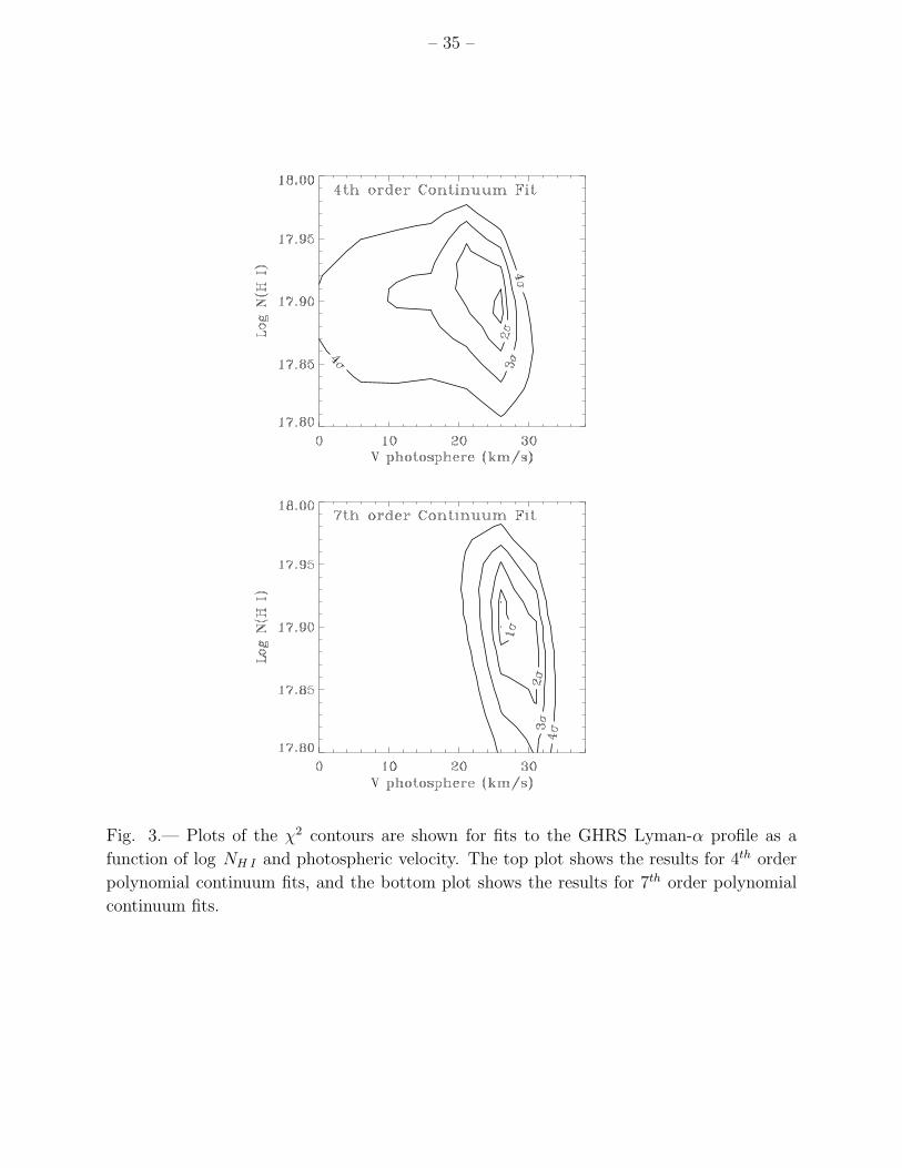
– 35 –

Fig. 3.— Plots of the χ2 contours are shown for fits to the GHRS Lyman-α profile as a

function of log NH I and photospheric velocity. The top plot shows the results for 4th order

polynomial continuum fits, and the bottom plot shows the results for 7th order polynomial

continuum fits.

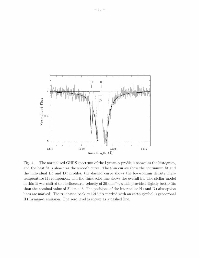
– 36 –

Fig. 4.— The normalized GHRS spectrum of the Lyman-α profile is shown as the histogram,

and the best fit is shown as the smooth curve. The thin curves show the continuum fit and

the individual H i and D i profiles; the dashed curve shows the low-column density high-

temperature H i component; and the thick solid line shows the overall fit. The stellar model

in this fit was shifted to a heliocentric velocity of 26 km s−1, which provided slightly better fits

than the nominal value of 21 km s−1. The positions of the interstellar H i and D i absorption

lines are marked. The truncated peak at 1215.6A marked with an earth symbol is geocoronal

H i Lyman-α emission. The zero level is shown as a dashed line.

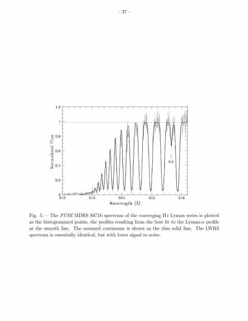
– 37 –

Fig. 5.— The FUSE MDRS SiC1b spectrum of the converging H i Lyman series is plotted

as the histogrammed points, the profiles resulting from the best fit to the Lyman-α profile

as the smooth line. The assumed continuum is shown as the thin solid line. The LWRS

spectrum is essentially identical, but with lower signal to noise.

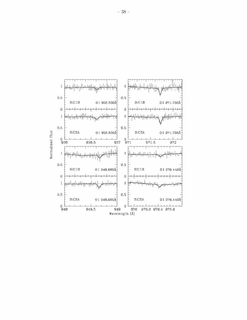
– 38 –

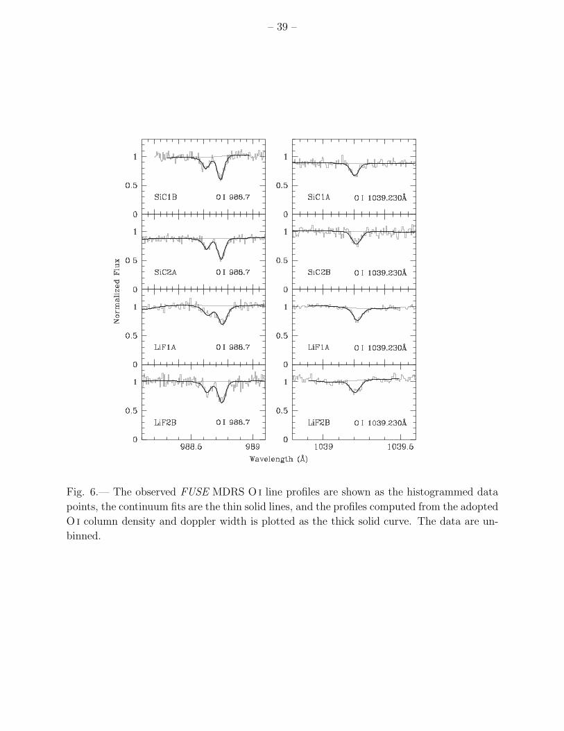
– 39 –

Fig. 6.— The observed FUSE MDRS O i line profiles are shown as the histogrammed data

points, the continuum fits are the thin solid lines, and the profiles computed from the adopted

O i column density and doppler width is plotted as the thick solid curve. The data are un-

binned.

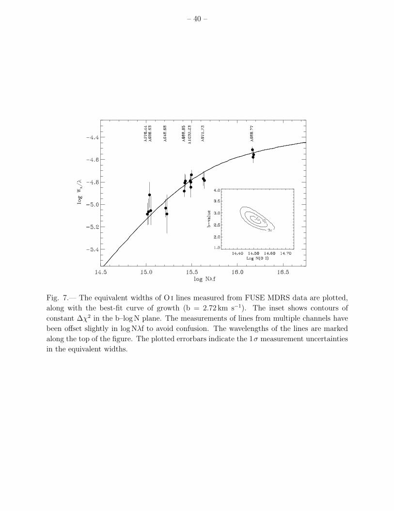
– 40 –

Fig. 7.— The equivalent widths of O i lines measured from FUSE MDRS data are plotted,

along with the best-fit curve of growth (b = 2.72 km s−1). The inset shows contours of

constant ∆χ2 in the b–logN plane. The measurements of lines from multiple channels have

been offset slightly in logNλf to avoid confusion. The wavelengths of the lines are marked

along the top of the figure. The plotted errorbars indicate the 1σ measurement uncertainties

in the equivalent widths.

– 41 –

Fig. 8.— The FUSE MDRS N i line profiles are shown as the thin histogram and the best

fit is shown as the thick solid line. The continuum fit is the thin smooth line. The SiC data

have been binned by two pixels for plotting purposes.

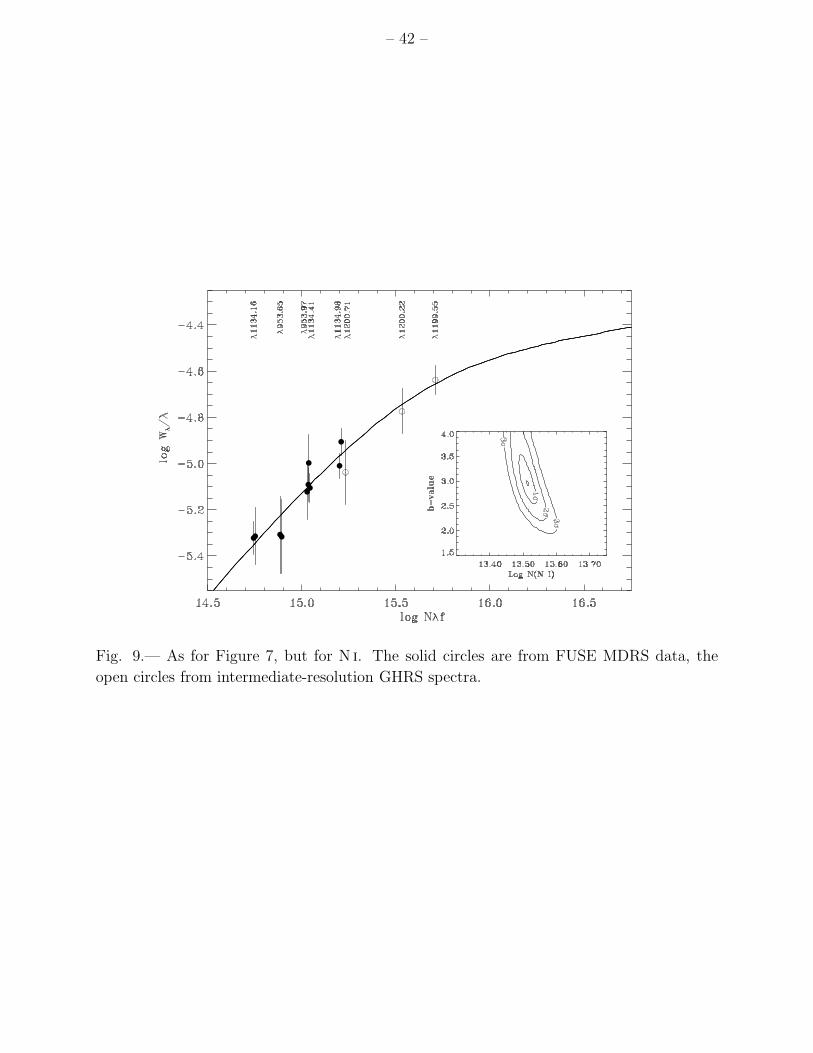
– 42 –

Fig. 9.— As for Figure 7, but for N i. The solid circles are from FUSE MDRS data, the

open circles from intermediate-resolution GHRS spectra.

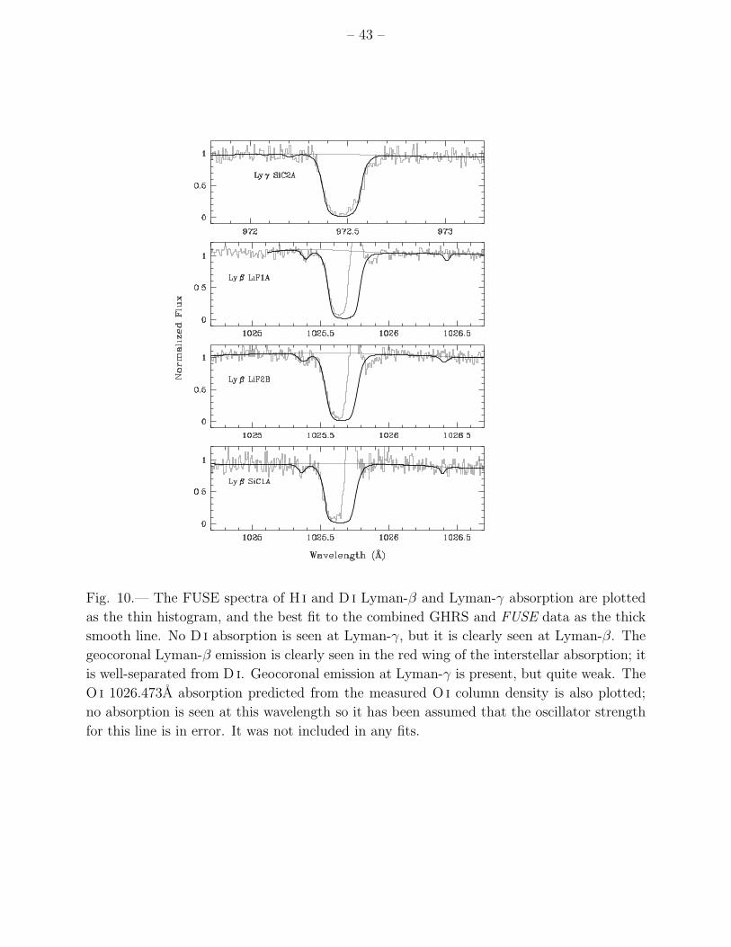
– 43 –

Fig. 10.— The FUSE spectra of H i and D i Lyman-β and Lyman-γ absorption are plotted

as the thin histogram, and the best fit to the combined GHRS and FUSE data as the thick

smooth line. No D i absorption is seen at Lyman-γ, but it is clearly seen at Lyman-β. The

geocoronal Lyman-β emission is clearly seen in the red wing of the interstellar absorption; it

is well-separated from D i. Geocoronal emission at Lyman-γ is present, but quite weak. The

O i 1026.473A absorption predicted from the measured O i column density is also plotted;

no absorption is seen at this wavelength so it has been assumed that the oscillator strength

for this line is in error. It was not included in any fits.

– 44 –

Fig. 11.— The FUSE MDRS N ii line profiles are shown as the thin histogram and the best fit

is shown as the thick solid line. The continuum fit is the thin smooth line. The neighboring

interstellar H i line profiles are labelled with tick marks in the plot of the 915.663Aline.

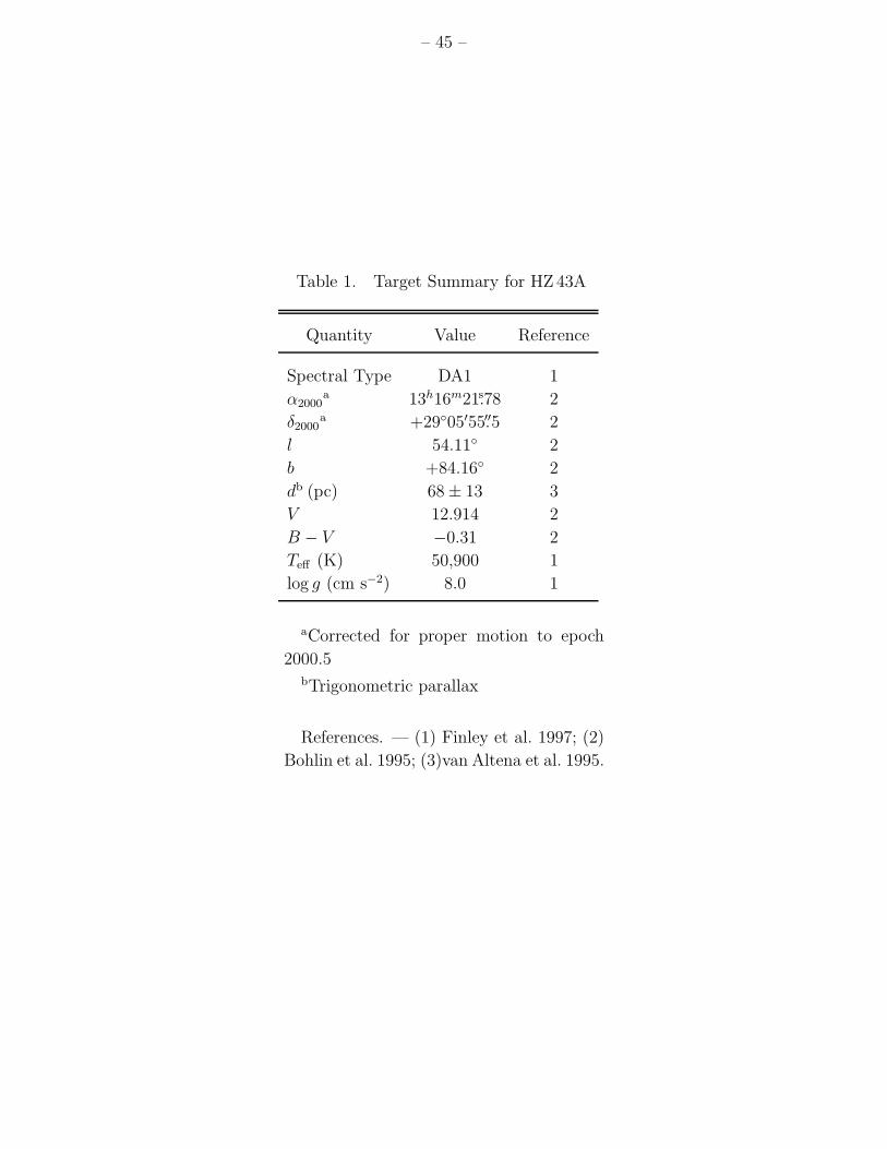
– 45 –

Table 1. Target Summary for HZ 43A

Quantity Value Reference

Spectral Type DA1 1

α2000a 13h16m21.s78 2

δ2000a +29◦05′55.′′5 2

l 54.11◦ 2

b +84.16◦ 2

db (pc) 68± 13 3

V 12.914 2

B − V −0.31 2

Teff (K) 50,900 1

log g (cm s−2) 8.0 1

aCorrected for proper motion to epoch

2000.5bTrigonometric parallax

References. — (1) Finley et al. 1997; (2)

Bohlin et al. 1995; (3)van Altena et al. 1995.

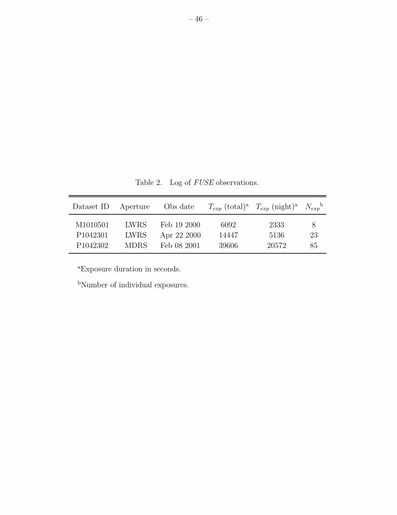
– 46 –

Table 2. Log of FUSE observations.

Dataset ID Aperture Obs date Texp (total)a Texp (night)a Nexpb

M1010501 LWRS Feb 19 2000 6092 2333 8

P1042301 LWRS Apr 22 2000 14447 5136 23

P1042302 MDRS Feb 08 2001 39606 20572 85

aExposure duration in seconds.

bNumber of individual exposures.

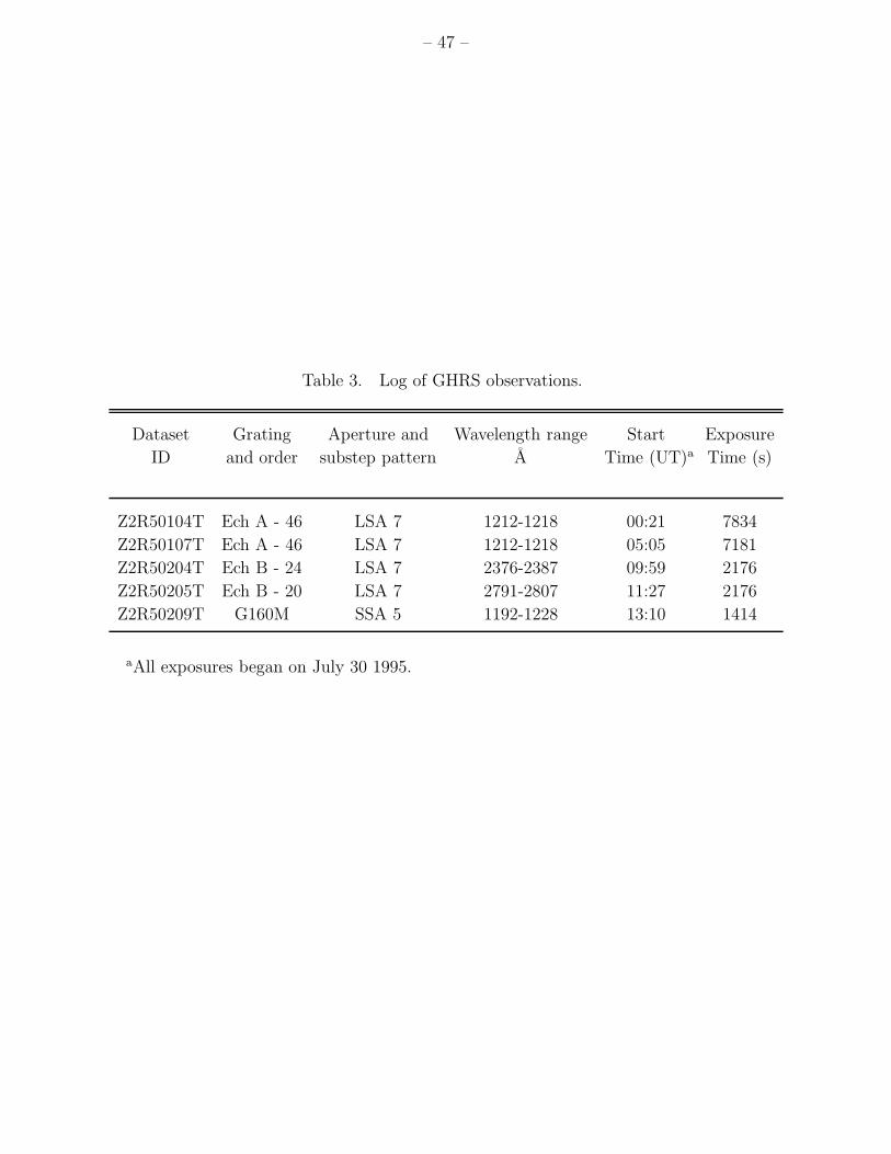
– 47 –

Table 3. Log of GHRS observations.

Dataset Grating Aperture and Wavelength range Start Exposure

ID and order substep pattern A Time (UT)a Time (s)

Z2R50104T Ech A - 46 LSA 7 1212-1218 00:21 7834

Z2R50107T Ech A - 46 LSA 7 1212-1218 05:05 7181

Z2R50204T Ech B - 24 LSA 7 2376-2387 09:59 2176

Z2R50205T Ech B - 20 LSA 7 2791-2807 11:27 2176

Z2R50209T G160M SSA 5 1192-1228 13:10 1414

aAll exposures began on July 30 1995.

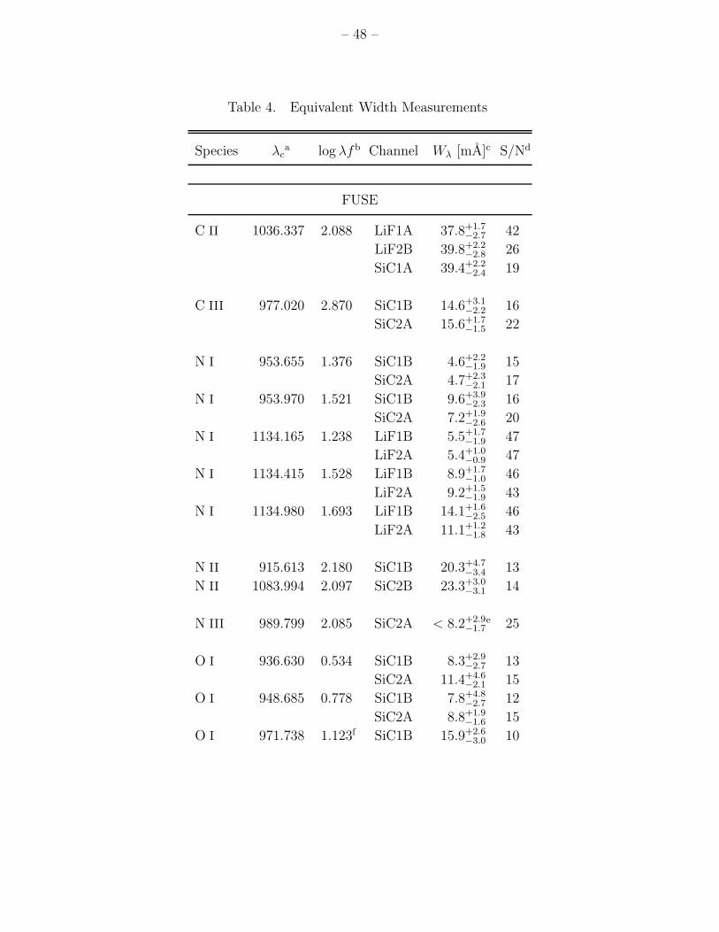
– 48 –

Table 4. Equivalent Width Measurements

Species λca log λfb Channel Wλ [mA]c S/Nd

FUSE

C II 1036.337 2.088 LiF1A 37.8+1.7−2.7 42

LiF2B 39.8+2.2−2.8 26

SiC1A 39.4+2.2−2.4 19

C III 977.020 2.870 SiC1B 14.6+3.1−2.2 16

SiC2A 15.6+1.7−1.5 22

N I 953.655 1.376 SiC1B 4.6+2.2−1.9 15

SiC2A 4.7+2.3−2.1 17

N I 953.970 1.521 SiC1B 9.6+3.9−2.3 16

SiC2A 7.2+1.9−2.6 20

N I 1134.165 1.238 LiF1B 5.5+1.7−1.9 47

LiF2A 5.4+1.0−0.9 47

N I 1134.415 1.528 LiF1B 8.9+1.7−1.0 46

LiF2A 9.2+1.5−1.9 43

N I 1134.980 1.693 LiF1B 14.1+1.6−2.5 46

LiF2A 11.1+1.2−1.8 43

N II 915.613 2.180 SiC1B 20.3+4.7−3.4 13

N II 1083.994 2.097 SiC2B 23.3+3.0−3.1 14

N III 989.799 2.085 SiC2A < 8.2+2.9−1.7

e 25

O I 936.630 0.534 SiC1B 8.3+2.9−2.7 13

SiC2A 11.4+4.6−2.1 15

O I 948.685 0.778 SiC1B 7.8+4.8−2.7 12

SiC2A 8.8+1.9−1.6 15

O I 971.738 1.123f SiC1B 15.9+2.6−3.0 10

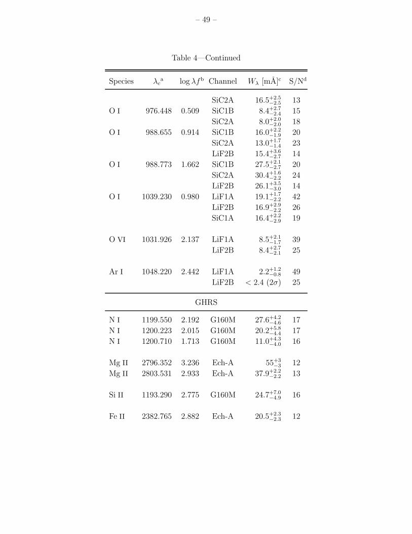
– 49 –

Table 4—Continued

Species λca log λfb Channel Wλ [mA]c S/Nd

SiC2A 16.5+2.5−2.5 13

O I 976.448 0.509 SiC1B 8.4+2.7−2.4 15

SiC2A 8.0+2.0−2.0 18

O I 988.655 0.914 SiC1B 16.0+2.2−1.9 20

SiC2A 13.0+1.7−1.4 23

LiF2B 15.4+3.6−2.7 14

O I 988.773 1.662 SiC1B 27.5+2.1−2.7 20

SiC2A 30.4+1.6−2.2 24

LiF2B 26.1+3.5−3.0 14

O I 1039.230 0.980 LiF1A 19.1+1.7−2.2 42

LiF2B 16.9+2.9−2.2 26

SiC1A 16.4+2.2−2.9 19

O VI 1031.926 2.137 LiF1A 8.5+2.1−1.7 39

LiF2B 8.4+2.7−2.1 25

Ar I 1048.220 2.442 LiF1A 2.2+1.2−0.8 49

LiF2B < 2.4 (2σ) 25

GHRS

N I 1199.550 2.192 G160M 27.6+4.2−4.6 17

N I 1200.223 2.015 G160M 20.2+5.8−4.4 17

N I 1200.710 1.713 G160M 11.0+4.3−4.0 16

Mg II 2796.352 3.236 Ech-A 55+3−3 12

Mg II 2803.531 2.933 Ech-A 37.9+2.2−2.2 13

Si II 1193.290 2.775 G160M 24.7+7.0−4.9 16

Fe II 2382.765 2.882 Ech-A 20.5+2.3−2.3 12

– 50 –

Table 4—Continued

Species λca log λfb Channel Wλ [mA]c S/Nd

aCentral wavelength of each transition from Mor-

ton 2001.bAdopted product of wavelength and oscillator

strength for each transition, taken from Morton

2001.cMeasured equivalent width and 1σ uncertainties

(in mA). The uncertainties contain contributions

from both statistical and systematic error sources.

dEmpirically estimated signal-to-noise ratios (per

unbinned pixel) for continuum regions near the ab-

sorption lines of interest.

eThe N III absorption contains a substantial con-

tribution from Si II at 989.873 (≈ +21 km s−1 from

the center of the N III line). The equivalent width

quoted may be dominated by the latter, but rep-

resents a firm upper limit for the amount of N IIIalong the HZ 43A sight line.

fThis transition is a blend of three O I lines, the

sum of whose oscillator strengths are given here.

– 51 –

Table 5. Curve of Growth Column Densities

Species log N ± 2σa b± 2σb ∆ log N c

C II 14.83+0.17−0.34

d,e +1.20

C III 12.59+0.09−0.10

d +0.15

N I 13.51+0.06−0.05 3.0+1.4

−0.7 · · ·N II 13.62+0.13

−0.17d +0.32

N III < 12.98+0.22−0.25

d +0.07

O I 14.51+0.07−0.06 2.72+0.33

−0.26 · · ·O VI 12.91+0.08

−0.08 ∞f · · ·Si II 12.85+0.18

−0.22d +0.21

Ar I 11.96+0.30−0.50

d +0.00

Mg II 12.41±0.02 2.8±0.3 · · ·Fe II 12.17±0.04 2.78±1.15 · · ·

aLog of column density derived from a curve

of growth fit, with estimated 2σ uncertainties.

For most species not enough transitions were

observed to independently fit a curve of growth

and determine a b-value. In these cases we have

adopted the b-value of 2.72+0.33−0.26 (2σ) from O I.

bDoppler parameter in km s−1 with esti-

mated 2σ uncertainties.cFor those species for which we have adopted

the b-value from O I we give the amount by

which the curve-of-growth-corrected column

density given in column 2 of this table exceeds

the average integrated apparent column den-

sity.

dWe have adopted the b-value of 2.72+0.33−0.26

(2σ) from O I to estimate the total column

density of these species.

eFor C II the b-value is probably larger, and

logN correspondingly smaller. Column 4 gives

the maximum correction for this effect.fFor O VI we assume that the instrument

fully-resolves the absorption profile and adopt

the weighted average of the apparent column

density integrations from the two LiF channels.

– 52 –

Table 6. HZ 43 Column Densities and Ratiosa

H i D i O i N i

Log N 17.93 ± 0.06 13.15+0.040−0.045 14.49 ± 0.08 13.51 ± 0.06

Ratios

D i/H i O i/H i N i/H i D i/O i D i/N i

1.66± 0.28× 10−5 3.63± 0.84× 10−4 3.80± 0.74× 10−5 4.57± 0.96× 10−2 4.37± 0.74× 10−1

aall uncertainties are 2 σ