AC 2011-1792: CONNECTING MASS AND ENERGY BALANCES TO THECONTINUUM SCALE WITH COMSOL DEMOS

Adrienne R. Minerick, Michigan Technological University

Adrienne Minerick is an Associate Professor of Chemical Engineering at Michigan Tech having movedfrom Mississippi State University in Jan 2010, where she was a tenured Associate Professor. She receivedher M.S. and Ph.D. from the University of Notre Dame in 2003 and B.S. from Michigan TechnologicalUniversity in 1998. Adrienne’s research interests include electrokinetics and the development of biomedi-cal microdevices. She earned a 2007 NSF CAREER award; her group has published in the Proceedings ofthe National Academy of Science, Lab on a Chip, and had an AIChE Journal cover. She is an active men-tor of undergraduate researchers and served as co-PI on an NSF REU site. Research within her Medicalmicro-Device Engineering Research Laboratory (M.D. ERL) also inspires the development of DesktopExperiment Modules (DEMos) for use in chemical engineering classrooms or as outreach activities inarea schools. Adrienne has been an active member of ASEE’s WIED, ChED, and NEE leadership teamssince 2003.

Jason M. Keith, Michigan Technological University

Jason Keith is an Associate Professor of Chemical Engineering at Michigan Technological University. Hereceived his B.S.ChE from the University of Akron in 1995, and his Ph.D from the University of NotreDame in 2001. He is the 2008 recipient of the Raymond W. Fahien Award for Outstanding TeachingEffectiveness and Educational Scholarship as well as a 2010 inductee into the Michigan TechnologicalUniversity Academy of Teaching Excellence. His current research interests include reactor stability, al-ternative energy, and engineering education. He is active within ASEE.

Faith A. Morrison, Michigan Technological University

Faith Morrison is an Associate Professor of Chemical Engineering at Michigan Technological Universityand currently the President of The Society of Rheology. She has authored a textbook on rheology and willsoon publish a textbook on introductory fluid mechanics.

Maria Fernanda TafurAytug Gencoglu, Michigan Technological University

Aytug Gencoglu received his BS in Chemical Engineering from Istanbul Technical University in 2003 andhis MS in Molecular Biology, Genetics and Biotechnology from Istanbul Technical University in 2005.He is currently a PhD candidate in Chemical Engineering in Michigan Technological University.

c©American Society for Engineering Education, 2011

Connecting Mass and Energy Balances to the Continuum Scale with COMSOL DEMo’s

Abstract In transport phenomena courses, students often struggle with the visualization of mass, momentum, and heat transfer. In this paper, we use COMSOL Multiphysics® to develop modules to help students connect high-level mass, momentum, and energy balances with the underlying physical phenomenon at the continuum scale. These modules are part of a larger project of Desktop Experiment Modules (DEMos) that enable students to experiment to deduce cause / effect in a demonstration tool. We focus on microfluidics and fuel cells because few examples exist in the chemical engineering literature in this area. These modules were implemented in chemical engineering in a special microdevice course for undergraduate upper-classmen and beginning graduate students, a senior level elective course on Computational Methods, and a junior-level transport / unit operations course. Introduction and Motivation: The Typical Transport Course Transport phenomena is a subject of the chemical engineering undergraduate curriculum that is taught in widely differing ways, depending upon the institution and its focus. In general, courses in fluid mechanics, heat transfer, and mass transfer can be categorized as:

1. Transport phenomena approach – in this approach, instructors focus on theoretical derivation of microscopic conservation equations and methods for obtaining analytical (and sometimes numerical) solutions. A typical book is that Bird, Stewart, and Lightfoot1.

2. Unit operations approach – in this approach, instructors focus on the practical use of macroscopic balance equations and using them for the design of pumps, heat exchangers, and membranes. A typical book is that of McCabe, Smith, and Harriott2.

3. A balance between the transport phenomena and unit operations approaches, such as that contained in the text of Geankoplis3.

At Michigan Technological University, students must complete a two-semester sequence of lecture courses (CM 3110 Transport / Unit Operations 1; CM 3120 Transport / Unit Operations 2). Based upon the title of the course we typically follow the third classification; however, content can vary depending on the instructor. Nevertheless, we have found that our hands-on students typically do well with the practical unit operations problems but struggle with the mathematics and conceptualization of transport theory. The literature supports our observations. For example, Krantz4 noted that transport texts analyze simple problems with analytical or basic numerical solutions. He then discusses the utility of computationally-based software to allow instructors of transport phenomena to focus on model development by introducing more complex problems. An additional

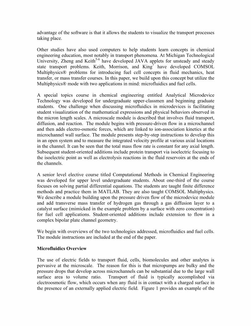
advantage of the software is that it allows the students to visualize the transport processes taking place. Other studies have also used computers to help students learn concepts in chemical engineering education, most notably in transport phenomena. At Michigan Technological University, Zheng and Keith5-6 have developed JAVA applets for unsteady and steady state transport problems. Keith, Morrison, and King7 have developed COMSOL Multiphysics® problems for introducing fuel cell concepts in fluid mechanics, heat transfer, or mass transfer courses. In this paper, we build upon this concept but utilize the Multiphysics® mode with two applications in mind: microfluidics and fuel cells. A special topics course in chemical engineering entitled Analytical Microdevice Technology was developed for undergraduate upper-classmen and beginning graduate students. One challenge when discussing microfluidics in microdevices is facilitating student visualization of the mathematical expressions and physical behaviors observed in the micron length scales. A microscale module is described that involves fluid transport, diffusion, and reaction. The module begins with pressure-driven flow in a microchannel and then adds electro-osmotic forces, which are linked to ion-association kinetics at the microchannel wall surface. The module presents step-by-step instructions to develop this in an open system and to measure the integrated velocity profile at various axial locations in the channel. It can be seen that the total mass flow rate is constant for any axial length. Subsequent student-oriented additions include protein transport via isoelectric focusing to the isoelectric point as well as electrolysis reactions in the fluid reservoirs at the ends of the channels. A senior level elective course titled Computational Methods in Chemical Engineering was developed for upper level undergraduate students. About one-third of the course focuses on solving partial differential equations. The students are taught finite difference methods and practice them in MATLAB. They are also taught COMSOL Multiphysics. We describe a module building upon the pressure driven flow of the microdevice module and add transverse mass transfer of hydrogen gas through a gas diffusion layer to a catalyst surface (mimicked in the example problem by a surface with zero concentration) for fuel cell applications. Student-oriented additions include extension to flow in a complex bipolar plate channel geometry. We begin with overviews of the two technologies addressed, microfluidics and fuel cells. The module instructions are included at the end of the paper. Microfluidics Overview The use of electric fields to transport fluid, cells, biomolecules and other analytes is pervasive at the microscale. The reason for this is that micropumps are bulky and the pressure drops that develop across microchannels can be substantial due to the large wall surface area to volume ratio. Transport of fluid is typically accomplished via electroosmotic flow, which occurs when any fluid is in contact with a charged surface in the presence of an externally applied electric field. Figure 1 provides an example of the

wall’s ion dissociation behavior in the presence of an electrolyte. A Debye layer forms near the wall that is dominated by counterions of opposite charge to the fixed wall charges. When an electric field is applied, these counterions and the water molecules associated with them are pulled uniformly toward the oppositely charged electrode. This drags the fluid along in a flat velocity profile. Note that the length scale of the Debye layer is on the order of hundreds of nanometers and the channel diameters are on the order of tens of microns or less.

Figure 1: Schematic of the surface chemical groups of a fused silica capillary in contact with a) air, b) an electrolyte, and c) an electrolyte and a remotely applied DC electric field. Figure 1 assumes an ideal, uniformly charged channel wall. However, the Debye layer is a function of electrolyte concentration via the Smoluchowski slip velocity at the wall:

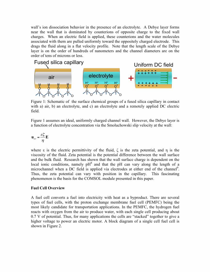
where ε is the electric permittivity of the fluid, ζ is the zeta potential, and η is the viscosity of the fluid. Zeta potential is the potential difference between the wall surface and the bulk fluid. Research has shown that the wall surface charge is dependent on the local ionic conditions, namely pH8 and that the pH can vary along the length of a microchannel when a DC field is applied via electrodes at either end of the channel9. Thus, the zeta potential can vary with position in the capillary. This fascinating phenomenon is the basis for the COMSOL module presented in this paper. Fuel Cell Overview A fuel cell converts a fuel into electricity with heat as a byproduct. There are several types of fuel cells, with the proton exchange membrane fuel cell (PEMFC) being the most likely candidate for transportation applications. In the PEMFC, the hydrogen fuel reacts with oxygen from the air to produce water, with each single cell producing about 0.7 V of potential. Thus, for many applications the cells are “stacked” together to give a higher voltage to power an electric motor. A block diagram of a single cell fuel cell is shown in Figure 2.

Figure 2. Schematic of one cell of a proton exchange membrane fuel cell. The slanted lines are the bipolar plates, the horizontal lines are the gas diffusion layer, the vertical lines are the electrodes (left block is the anode; right block is the cathode), and the grid represents the electrolyte. Within this single cell are bipolar plates which separate one cell from the other. The bipolar plates also have channels etched on either side to allow for reactant and product gases to flow. The plates need to have particular physical properties: low hydrogen permeation, high thermal conductivity, and high electrical conductivity. As the gases flow through the channels they undergo transverse diffusion to a gas diffusion layer. The gases are transported through this layer to reach the electrodes. In the PEMFC, the electrodes use a platinum catalyst to convert hydrogen into protons and electrons. The protons pass through a sulfonated polymer electrolyte membrane. Meanwhile, the electrons are conducted back through the gas diffusion layer, bipolar plate, and electric load where they react with the protons and oxygen to form water. For more information regarding fuel cell construction, please see the text of Larminie and Dicks10. Finite Element Problems In this paper we develop two modules in the following areas:

• Electrokinetics o This module solves the fluid flow (momentum) conservation equation in a

rectangular micro channel. The physics for this is ‘Laminar Flow’ with the simplification of ‘Incompressible Flow’.

o The electrokinetic forces are included by using an ‘Electroosmotic Velocity’ boundary condition at the walls. This uses the Smoluchowski slip velocity for which the zeta potential between the wall and the fluid can be defined. Behind the scenes, COMSOL is relying on the electrostatics physics.

Bipolar Plate Gas Diffusion Layer Anode Electrolyte

Bipolar Plate Gas Diffusion Layer Cathode

o The do-it-yourself portion of this module asks the students to alter the wall zeta potential such that it varies linearly between the anode and the cathode. Further, cause and effect case studies are required of the students.

• Fuel Cells o The first portion of this module solves the fluid flow (momentum)

conservation equation in a rectangular channel. o The second portion of this module adds mass transfer to the walls of the

rectangular channel (with zero species concentration) to mimic a large reaction of hydrogen to product

o The do-it-yourself portion of this module asks the students to reproduce the prior portions of the module to a serpentine geometry

Typical problems, shown here as separate appendices, walk the user through an example so they can become acquainted with how the software works. At the conclusion of the modules there is often a question or portion where the users apply their knowledge to a more complex problem that usually cannot be solved analytically. Conclusions We present ready-to-use modules using COMSOL Multiphysics® finite element software to build off fundamental concepts taught in the undergraduate transport courses. The modules are used by Michigan Technological University in elective courses, but they can easily be integrated into momentum, heat, or mass transfer courses. Students using the finite element method benefit from enhanced visualization of the physical processes occurring and also benefit from seeing practical applications of the complex partial differential equations that are typically derived in these courses. Acknowledgments The authors would like to acknowledge the National Science Foundation (NSF CBET #0644538) and the Department of Energy (Award Number DE-FG36-08GO18108) for partial support of this project. References

1. Bird, R. B.; Stewart, W. E.; Lightfoot, E. N. Transport Phenomena, 2nd Edition, Wiley, New York, NY, 2002.

2. McCabe, W. L.; Smith, J. C.; Harriott, P. Unit Operations of Chemical Engineering, 6th Edition, McGraw-Hill, New York, NY, 2001.

3. Geankoplis, C. J.; Transport Processes and Separation Process Principles, 4th Edition, Prentice Hall, Upper Saddle River, NJ, 2003.

4. Kranz, W. B., “Pediment Graduate Course in Transport Phenomena,” Proceedings of the 2003 American Society for Engineering Education Annual Conference & Exhibition.

5. Zheng, H.; Keith, J. M. “JAVA-Based Heat Transfer Visualization Tools,” Chemical Engineering Education, 38, 282 (2004).

6. Zheng, H.; Keith, J. M. “Web-Based Instructional Tools for Heat and Mass Transfer,” Proceedings of the 2003 American Society for Engineering Education Annual Conference & Exhibition.

7. Keith, J. M., Morrison, F. A., King, J. A.; “Finite Element Modules for Enhancing Undergraduate Transport Courses: Application to Fuel Cell Fundamentals,” Proceedings of the 2007 American Society for Engineering Education Annual Conference & Exhibition.

8. Minerick, A.R., A. Ostafin, and H.-C. Chang. "Electrokinetic Transport of Red Blood Cells in Micro-Capillaries," Electrophoresis, 23, 2165-2173, 2002.

9. Gencoglu, A, A. Ros, and A. R. Minerick, “Quantification of pH Gradients in DC-Dielectrophoretic Microdevice”, Special Dielectrophoresis Issue of Electrophoresis, submitted January 15, 2011.

10. Larminie, J.; Dicks, A. Fuel Cell Systems Explained, 2nd Edition, Wiley, West Sussex, England, 2003.

Appendix A: Using COMSOL Multiphysics® to Solve Engineering Modeling Problems: A Tutorial Appendix A.1: Fuel Cell Application

A classroom example which is designed to demonstrate fundamental concepts of COMSOL as well as the relationship between combined fluid flow and mass transfer in a fuel cell bipolar plate channel is described. COMSOL 4.0 is used for this example and assignment. The problem is modeled in a 2D geometry and the simulations are run to compute the stationary (steady-state) solution. These problems demonstrate the following concepts related to COMSOL to the students:

• The anatomy of a COMSOL model (Geometry, physics modules, mesh, boundaries and domains, computing, postprocessing)

• Selection of physics modules • Building geometries • Selecting boundary and initial conditions; use of expressions in boundary and

initial conditions, including position dependent expressions • Meshing • Generation of desired plots

In the first parts of this problem you will solve for laminar flow between two channels to simulate flow in a fuel cell bipolar plate.

Part 1: Select Problem Type Start-up

1. Click the Start button, point to All Programs → Other Apps →COMSOL 4.0a → COMSOL Multiphysics® 4.0a The program opens up in the Model Navigator

2. Select 2D from the Space Dimension drop-down list 3. Click the arrow for next page 4. Click the plus sign at the Fluid Flow Module, Single-Phase Flow, Laminar

Flow (spf). 5. Click the arrow for next page 6. Click the plus sing at the Present Studies and select Stationary. 7. Click the flag .

Part 2: Set up the Flow Geometry and Materials Geometry Setting

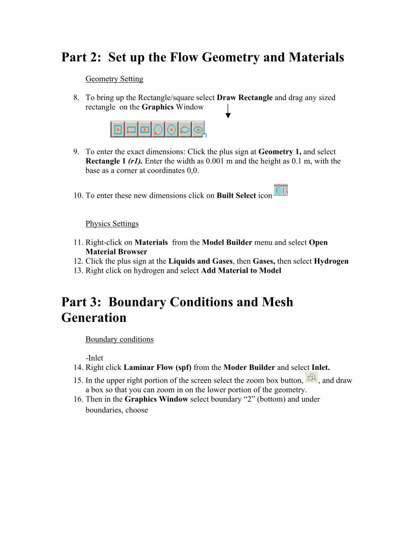
8. To bring up the Rectangle/square select Draw Rectangle and drag any sized rectangle on the Graphics Window

9. To enter the exact dimensions: Click the plus sign at Geometry 1, and select Rectangle 1 (r1). Enter the width as 0.001 m and the height as 0.1 m, with the base as a corner at coordinates 0,0.

10. To enter these new dimensions click on Built Select icon Physics Settings

11. Right-click on Materials from the Model Builder menu and select Open Material Browser

12. Click the plus sign at the Liquids and Gases, then Gases, then select Hydrogen 13. Right click on hydrogen and select Add Material to Model

Part 3: Boundary Conditions and Mesh Generation

Boundary conditions -Inlet

14. Right click Laminar Flow (spf) from the Moder Builder and select Inlet. 15. In the upper right portion of the screen select the zoom box button, , and draw

a box so that you can zoom in on the lower portion of the geometry. 16. Then in the Graphics Window select boundary “2” (bottom) and under

boundaries, choose

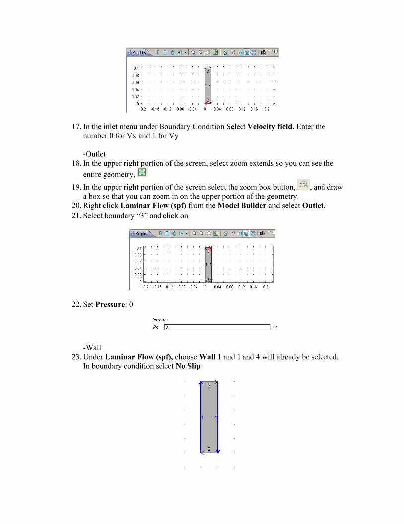
17. In the inlet menu under Boundary Condition Select Velocity field. Enter the number 0 for Vx and 1 for Vy

-Outlet

18. In the upper right portion of the screen, select zoom extends so you can see the entire geometry,

19. In the upper right portion of the screen select the zoom box button, , and draw a box so that you can zoom in on the upper portion of the geometry.

20. Right click Laminar Flow (spf) from the Model Builder and select Outlet. 21. Select boundary “3” and click on

22. Set Pressure: 0

-Wall 23. Under Laminar Flow (spf), choose Wall 1 and 1 and 4 will already be selected.

In boundary condition select No Slip

Mesh Generation

24. Right click on Mesh 1 from The Model Builder menu and select Free Triangular Mesh

25. In Model builder select Size, then Custom, then 0.00025 m 26. Under Mesh 1, right click on Free Triangular and select Build Selected

Part 4: Solve

27. In Model Builder, Study 1 right click on and select Compute.

Part 5: Generate Plots and Visualize the Solution

Arrow Surface

28. In results: Click the plus sign at 2D Plot Group 1 and select Surface 1. 29. Right click on Surface 1 and select Disable to clean the plot view 30. Right click on 2D Plot Group 1 from The Model Builder menu and select

Arrow Surface 31. Under Arrow Positioning select 9 points in x grid points and 15 points in y grid

points, and a scale factor of 0.2. Make sure you have selected solution 1.

32. Click on Plot to draw the arrow plot and see the parabolic velocity profile. You can zoom in if you need to see the arrows.

Velocity Profile Generation

33. Right click on Arrow Surface 1 and select Disable to clean the plot view 34. Right click on Data Sets and select Cut Line 2D

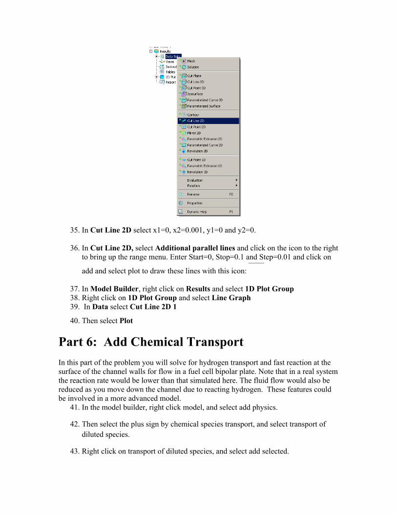
35. In Cut Line 2D select x1=0, x2=0.001, y1=0 and y2=0.

36. In Cut Line 2D, select Additional parallel lines and click on the icon to the right to bring up the range menu. Enter Start=0, Stop=0.1 and Step=0.01 and click on

add and select plot to draw these lines with this icon:

37. In Model Builder, right click on Results and select 1D Plot Group 38. Right click on 1D Plot Group and select Line Graph 39. In Data select Cut Line 2D 1

40. Then select Plot

Part 6: Add Chemical Transport In this part of the problem you will solve for hydrogen transport and fast reaction at the surface of the channel walls for flow in a fuel cell bipolar plate. Note that in a real system the reaction rate would be lower than that simulated here. The fluid flow would also be reduced as you move down the channel due to reacting hydrogen. These features could be involved in a more advanced model.

41. In the model builder, right click model, and select add physics.

42. Then select the plus sign by chemical species transport, and select transport of diluted species.

43. Right click on transport of diluted species, and select add selected.

44. Click on the flag, select domain 1, and click on the plus sign .

45. In the model builder, click on the plus next to transport of diluted species.

46. Right click on transport of diluted species, select convection and diffusion, highlight the domain (domain number 1 is the entire rectangle), select velocity field spf1/fp1, and enter a diffusion coefficient of 1 x 10-6 m2/s.

47. Right click on transport of diluted species, select inflow, and enter 41 mol/m3. Zoom in, select boundary 2, and click on the plus sign.

48. Right click on transport of diluted species, select concentration, and enter 0 mol/m3. Zoom in, select boundaries 1 and 4, and click on the plus sign. Use the control key to select multiple boundaries.

49. Right click on transport of diluted species and select outflow. Zoom in, select boundary 3, and click on the plus sign.

50. Right click on study, and select compute.

51. Right click on results and select 2D plot group.

52. Right click on the 2D plot group you just created, and select surface.

53. For data set, select solution 1.

54. In expression, right click, select transport of diluted species, and select species c,

and select concentration. Then click on the plot symbol .

55. Zoom in and determine the concentration at different locations axially in the channel.

Part 7: Do It Yourself Repeat this process with a complex hydrogen flow channel geometry, as seen below. Adjust the feed inlet velocity and look at the impact on the exit hydrogen concentration.

0.001 m 0.1 m 0.004 m

Appendix B.1: Microdevice Electroosmotic Flow Application A classroom example which is designed to demonstrate fundamental concepts of COMSOL as well as the relationship between the zeta potential and the electroosmotic velocity field in a microfluidic channel is described. Later, an assignment which is a variation of the classroom example is also described. COMSOL 4.0 is used for this example and assignment. Both problems are modeled in a 2D geometry and the simulations are run to compute the stationary (steady-state) solution. These problems demonstrate the following concepts related to COMSOL to the students:

• The anatomy of a COMSOL model (Geometry, physics modules, mesh, boundaries and domains, computing, postprocessing)

• Selection of physics modules • Building geometries • Selecting boundary and initial conditions; use of expressions in boundary and

initial conditions, including position dependent expressions • Meshing • Generation of desired plots

Part 1: Select Physics Module The classroom example problem consists of electroosmotic flow of water through a straight microfluidic channel with two sections that have different Zeta potentials. The electroosmotic flow velocity in the channel is given by the Smoluchowski slip velocity, which is independent of the position along the cross-section of the channel:

€

ueo =εζηE

where ε is the electric permittivity of the fluid, ζ is the zeta potential, and η is the viscosity of the fluid. Zeta potential is the potential difference between the wall surface and the bulk fluid. This example features two sections of a channel with different zeta potentials, which results in induced pressure gradients. So a physics interface which can model both pressure driven and electroosmotic flows is required.

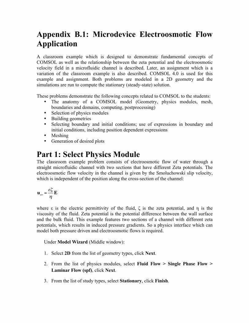
Under Model Wizard (Middle window): 1. Select 2D from the list of geometry types, click Next.

2. From the list of physics modules, select Fluid Flow > Single Phase Flow > Laminar Flow (spf), click Next.

3. From the list of study types, select Stationary, click Finish.

Part 2: Set Up the Geometry and Materials A straight microchannel modeled in 2D can be represented simply as a rectangle. However, this problem involves two sections with differing channel wall properties, which requires that sections of the channel walls are defined as separate boundaries. Thus, the channel will be modeled as two adjacent rectangles.

4. Under Model Builder (Left hand side window), select Geometry 1:

5. In the Settings tab (Center window), set the Length units to µm

6. Right-click Geometry 1 under Model Builder, select Rectangle

7. Set Width and Height to 250 and 20 µm, respectively, set base position to ‘Corner,’ X = 0, and Y = 0

8. Select Build All

9. Repeat Steps 2-4, but change the base position to ‘Corner,’ X = 250, and Y = 0

The resulting geometry includes two domains, which represent volumes and can be assigned different conditions. It also includes eight boundaries, one of which is an internal boundary (meaning it is a boundary between two domains). Boundaries represent the boundaries between two domains (volumes) if they are an internal boundary, or those between the system and the surroundings if they are not.

10. Either right-click on Materials under Model Builder and select Open Material Browser, or select the Material Browser tab in the middle window.

11. Select Built In > Water, liquid. Right click on the material’s name and select Add Material to Model.

Part 3: Boundary Conditions and Mesh Generation In COMSOL, most of the model building is done after physics interfaces are selected and the geometries are built. A description of the system and the problem is accomplished by defining boundary conditions at boundaries, initial values in domains, and relevant physical properties in both.

12. Under the Model Builder, click the triangle next to Laminar Flow (spf) to expand the physics interface:

13. Select Laminar Flow (spf) Set the Compressibility under Physical Model to ‘Incompressible flow.’

14. Select Fluid Properties 1 Set the Density (ρ) and Viscosity (µ) to From Material This instructs COMSOL to use the values defined in the selected material (‘Water, liquid’) for these properties.

15. Select Inlet. Select the left hand side boundary by clicking on it to highlight and right clicking to select. Choose Pressure, no viscous stress as the Boundary condition and set the pressure to 0 atm.

16. Select Outlet. Select the right hand side boundary by clicking on it to highlight and right clicking to select. Choose Pressure, no viscous stress as the Boundary condition and set the pressure to 0 atm.

17. Select Initial Values. Set the initial pressure to 0 atm.

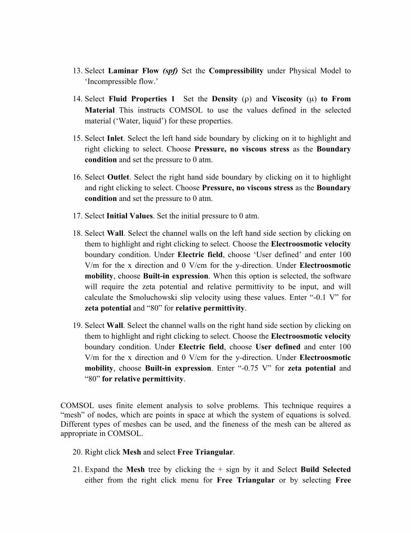
18. Select Wall. Select the channel walls on the left hand side section by clicking on them to highlight and right clicking to select. Choose the Electroosmotic velocity boundary condition. Under Electric field, choose ‘User defined’ and enter 100 V/m for the x direction and 0 V/cm for the y-direction. Under Electroosmotic mobility, choose Built-in expression. When this option is selected, the software will require the zeta potential and relative permittivity to be input, and will calculate the Smoluchowski slip velocity using these values. Enter “-0.1 V” for zeta potential and “80” for relative permittivity.

19. Select Wall. Select the channel walls on the right hand side section by clicking on them to highlight and right clicking to select. Choose the Electroosmotic velocity boundary condition. Under Electric field, choose User defined and enter 100 V/m for the x direction and 0 V/cm for the y-direction. Under Electroosmotic mobility, choose Built-in expression. Enter “-0.75 V” for zeta potential and “80” for relative permittivity.

COMSOL uses finite element analysis to solve problems. This technique requires a “mesh” of nodes, which are points in space at which the system of equations is solved. Different types of meshes can be used, and the fineness of the mesh can be altered as appropriate in COMSOL.

20. Right click Mesh and select Free Triangular.

21. Expand the Mesh tree by clicking the + sign by it and Select Build Selected either from the right click menu for Free Triangular or by selecting Free

Triangular and clicking the Build Selected icon at the top of the Free Triangular dialog window.

This gives a basic mesh which is adequate to solve this problem.

Part 4: Solve

22. Right click Study 1 and select Compute.

Part 5: Generate Plots and Visualize the Solution Plotting surface and arrow surface plots of velocities:

23. Once the problem is solved, expand the Results tree by clicking the + sign by it.

24. Right click 2D Plot Group and select Surface. This will add a surface plot to this plot group.

25. Select Surface and click the Replace expression icon in the corresponding dialog window. Select Laminar Flow>Velocity field magnitude and then click the Plot icon. A surface plot of the magnitude of the velocity vector will appear.

26. Right click 2D Plot Group and select Arrow surface to add an arrow surface plot to this plot group.

27. Select Arrow surface and click the Replace expression icon in the corresponding dialog window. Select Laminar flow>Velocity field>Velocity field, x-component and then click on the Plot icon. An arrow surface plot of the x-component of the velocity will be overlaid the surface plot. This will demonstrate the change in the cross-sectional velocity profile around the point where the zeta potential changes.

Plotting cross-sectional velocity profiles:

28. Right click Data Sets under Results and select Cut Line 2D.

29. Select Two point entry for Line entry method Enter (0,0) and (0,20) as the coordinates for the two points. Click Plot. A cut line between these points (Cross-section at the inlet, x = 0 µm) will be defined.

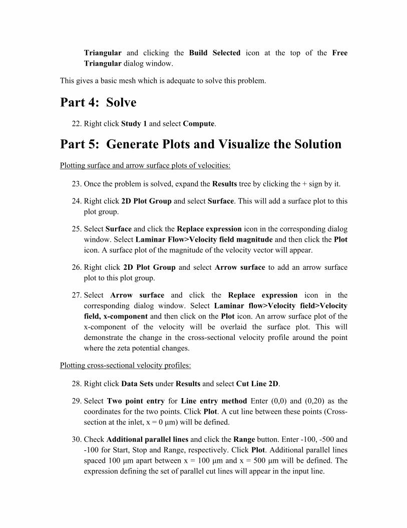
30. Check Additional parallel lines and click the Range button. Enter -100, -500 and -100 for Start, Stop and Range, respectively. Click Plot. Additional parallel lines spaced 100 µm apart between x = 100 µm and x = 500 µm will be defined. The expression defining the set of parallel cut lines will appear in the input line.

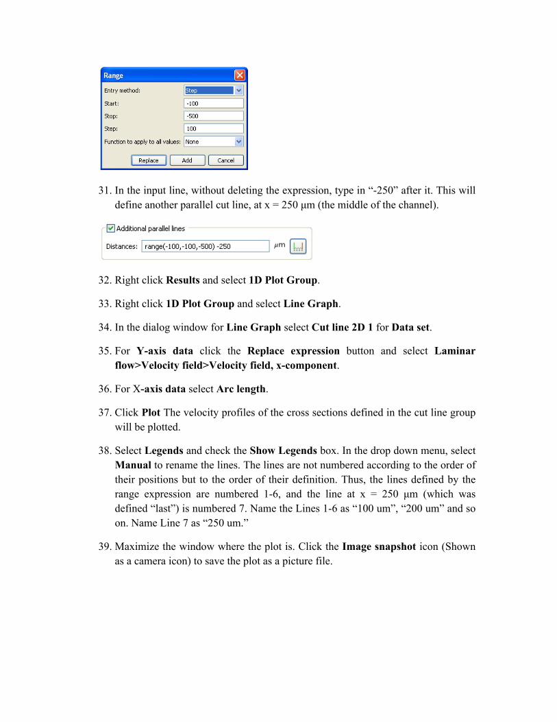
31. In the input line, without deleting the expression, type in “-250” after it. This will define another parallel cut line, at x = 250 µm (the middle of the channel).

32. Right click Results and select 1D Plot Group.

33. Right click 1D Plot Group and select Line Graph.

34. In the dialog window for Line Graph select Cut line 2D 1 for Data set.

35. For Y-axis data click the Replace expression button and select Laminar flow>Velocity field>Velocity field, x-component.

36. For X-axis data select Arc length.

37. Click Plot The velocity profiles of the cross sections defined in the cut line group will be plotted.

38. Select Legends and check the Show Legends box. In the drop down menu, select Manual to rename the lines. The lines are not numbered according to the order of their positions but to the order of their definition. Thus, the lines defined by the range expression are numbered 1-6, and the line at x = 250 µm (which was defined “last”) is numbered 7. Name the Lines 1-6 as “100 um”, “200 um” and so on. Name Line 7 as “250 um.”

39. Maximize the window where the plot is. Click the Image snapshot icon (Shown as a camera icon) to save the plot as a picture file.

Part 6: Export Data It was desired to integrate the cross-sectional velocity profiles to show that the mass flow rate does not change with the axial position. To do this, data must be exported from COMSOL.

40. Right click Report and select Data.

41. Under Data select Cut line 2D 1 for Data set.

42. Click the Replace expression button and select Laminar flow>Velocity field>Velocity field, x-component. This selects the velocity in the x-direction as the data that will be exported. The cut lines themselves are defined only as geometric entities, and no variable is associated with them.

43. Choose a filename and save location, and select Spreadsheet for Data format.

44. Click the Export button at the top of the dialog window.

A .txt file will be generated, which can be opened with Excel or a similar spreadsheet software.

Part 7: Do It Yourself As an assignment, students were asked to solve the same problem and create the same plots for the case of a different zeta potential profile. In this case, there were not to be two sections with different zeta potentials, but the zeta potential would change linearly along the axial direction. They were asked to run the simulation for three cases where the zeta potential changed linearly between three potential ranges of their choosing along the axial direction, and to generate the velocity surface and velocity (x-direction) arrow surface plots described above for each case. The step by step procedure for this version of the problem is almost identical to the one described above. Only the differences are described below:

1. The problem will work with the geometry described above, but it doesn’t require the two sections. To build the geometry, follow the same instructions as above, but only build one rectangle. Set Width and Height to 500 and 20 µm, respectively, set base position to ‘Corner,’ X = 0, and Y = 0.

2. When setting up the ‘Wall’ conditions for the channel walls, enter ‘-0.1-500*x’ for zeta potential. (Note that x is in m.) If using the same geometry as the class problem, selecting the walls in both sections of the channel and entering the same expression for zeta potential gives the same results.

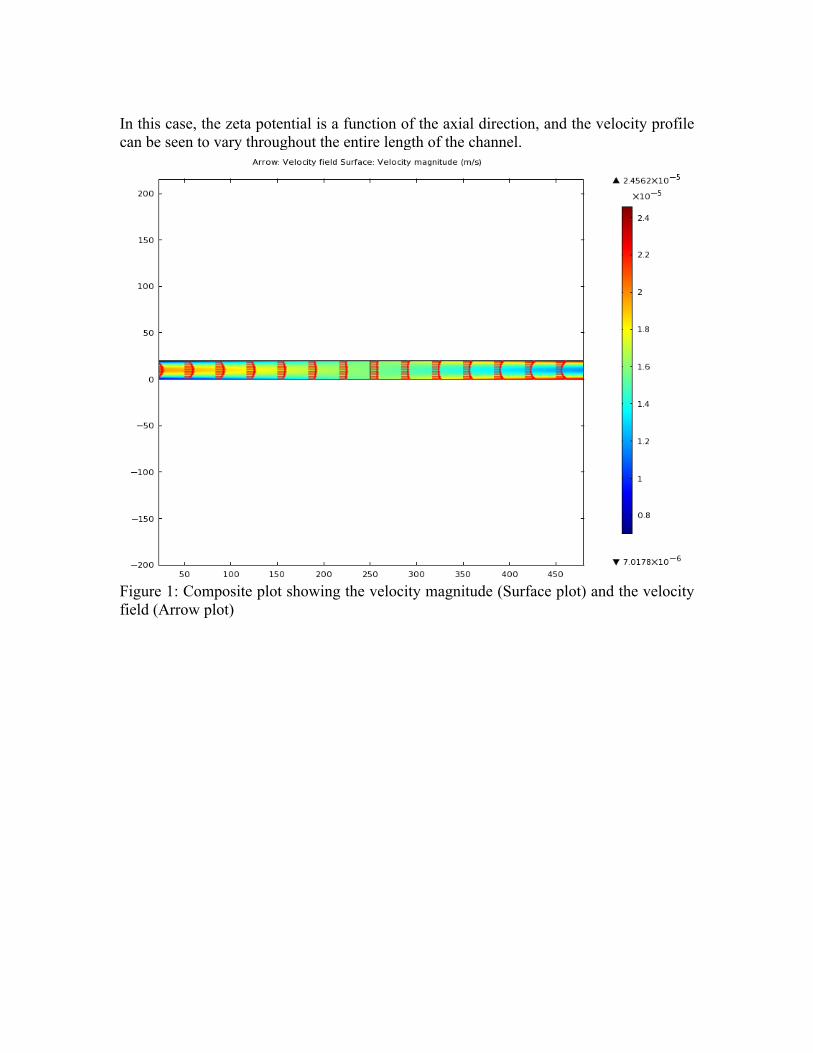
In this case, the zeta potential is a function of the axial direction, and the velocity profile can be seen to vary throughout the entire length of the channel.

Figure 1: Composite plot showing the velocity magnitude (Surface plot) and the velocity field (Arrow plot)

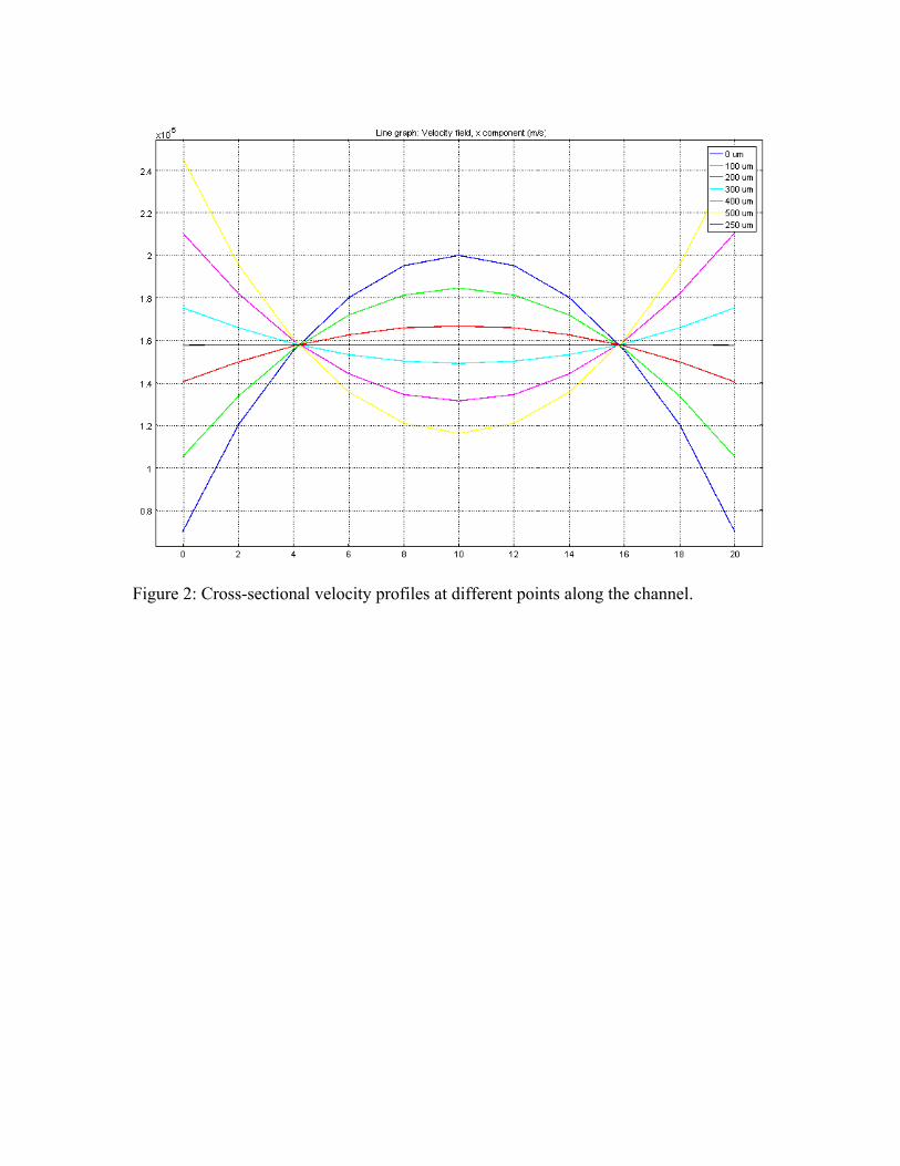
Figure 2: Cross-sectional velocity profiles at different points along the channel.