AC 2012-5478: FLEXIBLE MULTIBODY DYNAMICS EXPLICIT SOLVERFOR REAL-TIME SIMULATION OF AN ONLINE VIRTUAL DYNAMICSLAB

Mr. Hatem M. Wasfy, Advanced Science and Automation Corp.

Hatem Wasfy is the President of Advanced Science and Automation Corp. (ASA) a company that special-izes in the development of online virtual learning environments, and advanced engineering simulations.He has helped design several interactive learning environments that include a CNC machining course, acentrifugal pump maintenance course, an undergraduate physics course, and a welding course. He re-ceived a B.S. (1994) and an M.S. (1996) in mechanical engineering from the American University inCairo. Wasfy’s research interests include advanced learning systems, cavitation modeling, computationalfluid dynamics, internal combustion engine modeling and design, and AI rule-based expert systems.

Dr. Tamer M. Wasfy, Indiana University-Purdue University, Indianapolis

Tamer Wasfy received a B.S. (1989) in mechanical wngineering and an M.S. (1990) in materials engineer-ing from the American University in Cairo, and an M.Phil. (1993) and Ph.D. (1994) in mechanical engi-neering from Columbia University. He worked as a Research Scientist at the Department of MechanicalEngineering, Columbia University (1994-1995) and at the University of Virginia at NASA Langley Re-search Center (1995-1998). Wasfy is an Associate Professor at the Mechanical Engineering Department atIndiana University-Purdue University Indianapolis (IUPUI). Dr. Wasfy is also the founder and chairmanof Advanced Science and Automation Corp. (founded in 1998) and AscienceTutor (founded in 2007).Wasfy’s research and development areas include: flexible multibody dynamics, finite element modelingof solids and fluids, fluid-structure interaction, belt-drive dynamics, tires mechanics/dynamics, ground ve-hicle dynamics, visualization of numerical simulation results, engineering applications of virtual-reality,and artificial intelligence. He authored and co-authored more than 70 peer-reviewed publications and gavemore than 65 presentations at international conferences and invited lectures in those areas. He receivedtwo ASME best conference paper awards as first author. He is the software architect for the DIS, IVRESSand LEA software systems, which are used by industry, government agencies, and academic institutions.Wasfy is a member of ASME, AIAA, SAE, and ASEE.

Ms. Jeanne Peters, Advanced Science and Automation Corp.

Jeanne Peters received a B.A. in math/computer science from the College of William and Mary. Sheworked at NASA Langley Research Center in Hampton, Va. for more than 20 years as a Senior Program-mer/Analyst for George Washington University, University of Virginia, and Old Dominion University.She co-authored more than 70 journal and conference papers in the areas of computational mechanics,finite element method, shells/plates, composite material panels, and tires. She has also worked on nu-merous projects to create advanced engineering design and learning environments which include multi-modal user interfaces for space systems. As Vice President of Information Technology, Peters directs thedevelopment of advanced virtual reality applications, including scientific visualization applications andweb-based multimedia education/training applications.

c©American Society for Engineering Education, 2012

Page 25.641.1

Flexible Multibody Dynamics Explicit Solver for Real-Time Simulation of an

Online Virtual Dynamics Lab

Abstract

A high-fidelity online virtual video-game-like Newtonian dynamics lab that can be used as a

teaching lab for university freshman physics and sophomore engineering dynamics courses is

presented in this paper. The lab is driven using a virtual-reality display engine with an integrated

flexible multibody dynamics finite element explicit real-time solver. The hierarchical “scene-

graph” representation of the lab that is used in the virtual-reality display engine is also used in

the solver. The multibody system includes rigid bodies, flexible bodies, joints, frictional contact

constraints, actuators and controllers. Flexible bodies are modeled using spring, truss and beam

elements. A penalty technique is used to impose joint/contact constraints. An asperity-based

friction model is used to model joint/contact friction. A bounding box binary tree contact search

algorithm is used to allow fast contact detection between finite elements and other elements as

well as general triangular/quadrilateral rigid-body surfaces. The following experiments are

modeled: mass-spring systems, pendulums, pulley-rope-mass systems, air-hockey, billiards, 1D

and 2D frictional and frictionless motion with and without gravity, roller-coasters, planetary

motion, gears, cams, robotic manipulators and linkages.

1. Introduction

A flexible multibody system is a system of interconnected rigid and/or flexible bodies. The

bodies are connected using various types of joints including spherical, revolute, cylindrical,

prismatic, planar and screw joints. The bodies can come into contact with one-another or with

the surroundings. Virtual-reality applications require a real-time multibody dynamics engine in

order to allow users to interact with objects in the virtual-environment (VE) in a physically

accurate way. In the present paper we present the application of an advanced real-time flexible

multibody dynamics solver to simulate a dynamics lab that can be used in freshmen university

physics and sophomore engineering dynamics courses. The student can interact with the virtual

lab experiments using a user-friendly interface. For example, a typical Newton 2nd

law

experiment consisting of two vertically suspended masses connected by a rope and pulley is

shown in Figure 1. The student can set the value of the masses, then release the masses and

observe the motion of the masses. The motion of the masses is also plotted in graph. The student

can copy the graph data to a spreadsheet to do further analysis and to write a lab report. Another

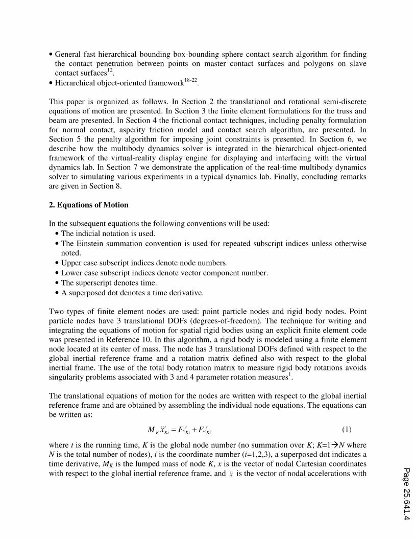
typical experiment is of a puck moving on 1-dimensional rail is shown in Figure 2. The student

can do various experiments by setting the inclination angle of the rail, the friction coefficient

between the rail and the puck, the initial position of the puck on the rail, and the initial velocity

of the puck. For example, by setting the inclination angle and the friction coefficient to zero, the

student can observe the motion of the puck due to an initial velocity. In this case the experiment

can be used to prove Newton’s first law of motion. Alternatively, the student can set the

inclination angle of the rail to 30 degrees and study the motion of the puck under the action of

gravity. Then the student can set the friction coefficient to say 0.3 and find the inclination angle

at which the puck starts moving, which is the friction angle.

Page 25.641.2

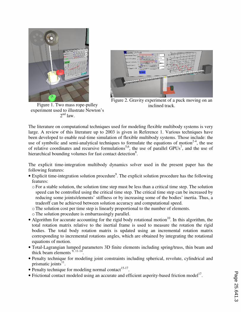
Figure 1. Two mass rope-pulley

experiment used to illustrate Newton’s

2nd

law.

Figure 2. Gravity experiment of a puck moving on an

inclined track.

The literature on computational techniques used for modeling flexible multibody systems is very

large. A review of this literature up to 2003 is given in Reference 1. Various techniques have

been developed to enable real-time simulation of flexible multibody systems. Those include: the

use of symbolic and semi-analytical techniques to formulate the equations of motion2-4

, the use

of relative coordinates and recursive formulations5,6

, the use of parallel GPUs7, and the use of

hierarchical bounding volumes for fast contact detection8.

The explicit time-integration multibody dynamics solver used in the present paper has the

following features:

• Explicit time-integration solution procedure9. The explicit solution procedure has the following

features:

o For a stable solution, the solution time step must be less than a critical time step. The solution

speed can be controlled using the critical time step. The critical time step can be increased by

reducing some joints/elements’ stiffness or by increasing some of the bodies’ inertia. Thus, a

tradeoff can be achieved between solution accuracy and computational speed.

o The solution cost per time step is linearly proportional to the number of elements.

o The solution procedure is embarrassingly parallel.

• Algorithm for accurate accounting for the rigid body rotational motion10

. In this algorithm, the

total rotation matrix relative to the inertial frame is used to measure the rotation the rigid

bodies. The total body rotation matrix is updated using an incremental rotation matrix

corresponding to incremental rotations angles, which are obtained by integrating the rotational

equations of motion.

• Total-Lagrangian lumped parameters 3D finite elements including spring/truss, thin beam and

thick beam elements 9, 11-14

.

• Penalty technique for modeling joint constraints including spherical, revolute, cylindrical and

prismatic joints11

.

• Penalty technique for modeling normal contact15-17

.

• Frictional contact modeled using an accurate and efficient asperity-based friction model17

.

Page 25.641.3

• General fast hierarchical bounding box-bounding sphere contact search algorithm for finding

the contact penetration between points on master contact surfaces and polygons on slave

contact surfaces12

.

• Hierarchical object-oriented framework18-22

.

This paper is organized as follows. In Section 2 the translational and rotational semi-discrete

equations of motion are presented. In Section 3 the finite element formulations for the truss and

beam are presented. In Section 4 the frictional contact techniques, including penalty formulation

for normal contact, asperity friction model and contact search algorithm, are presented. In

Section 5 the penalty algorithm for imposing joint constraints is presented. In Section 6, we

describe how the multibody dynamics solver is integrated in the hierarchical object-oriented

framework of the virtual-reality display engine for displaying and interfacing with the virtual

dynamics lab. In Section 7 we demonstrate the application of the real-time multibody dynamics

solver to simulating various experiments in a typical dynamics lab. Finally, concluding remarks

are given in Section 8.

2. Equations of Motion

In the subsequent equations the following conventions will be used:

• The indicial notation is used.

• The Einstein summation convention is used for repeated subscript indices unless otherwise

noted.

• Upper case subscript indices denote node numbers.

• Lower case subscript indices denote vector component number.

• The superscript denotes time.

• A superposed dot denotes a time derivative.

Two types of finite element nodes are used: point particle nodes and rigid body nodes. Point

particle nodes have 3 translational DOFs (degrees-of-freedom). The technique for writing and

integrating the equations of motion for spatial rigid bodies using an explicit finite element code

was presented in Reference 10. In this algorithm, a rigid body is modeled using a finite element

node located at its center of mass. The node has 3 translational DOFs defined with respect to the

global inertial reference frame and a rotation matrix defined also with respect to the global

inertial frame. The use of the total body rotation matrix to measure rigid body rotations avoids

singularity problems associated with 3 and 4 parameter rotation measures1.

The translational equations of motion for the nodes are written with respect to the global inertial

reference frame and are obtained by assembling the individual node equations. The equations can

be written as:

t

Kiat

Kist

KiK FFxM +=&& (1)

where t is the running time, K is the global node number (no summation over K; K=1�N where

N is the total number of nodes), i is the coordinate number (i=1,2,3), a superposed dot indicates a

time derivative, MK is the lumped mass of node K, x is the vector of nodal Cartesian coordinates

with respect to the global inertial reference frame, and x&& is the vector of nodal accelerations with

Page 25.641.4

respect to the global inertial reference frame, Fs is the vector of internal structural forces, and Fa

is the vector of externally applied forces, which include surface forces and body forces.

For each node representing a rigid body, a body-fixed material frame is defined. The origin of

the body frame is located at the node that is also the body’s center of mass. The mass of the body

is concentrated at that node and the inertia of the body is given by the inertia tensor defined with

respect to the body frame. The orientation of the body-frame is given by ot

KR which is the rotation

matrix relative to the global inertial frame at time t0. The rotational equations of motions are

written for each node with respect to its’ body-fixed material frames as:

( )Ki

t

KjKij

t

Ki

t

Kiat

Kist

KjKij ITTI )( θθθ &&&& ×−+= (2)

where IK is the inertia tensor of rigid body K, Kjθ&& and

Kjθ& are the angular acceleration and velocity

vectors’ components for rigid body K relative to its material frame in direction j (j=1,2,3), TsKi

are the components of the vector of internal torque at node K in direction i, and TaKi are the

components of the vector of applied torque. The summation convention is used only for the

lower case indices i and j. Since, the rigid body rotational equations of motion are written in a

body (material) frame, thus, the inertia tensor IK is constant.

The trapezoidal rule is used as the time integration formula for solving Equation (1) for the

global nodal positions x:

)(5.0 tt

Kj

t

Kj

tt

Kj

t

Kj xxtxx∆−∆− +∆+= &&&&&& (3a)

)(5.0 tt

Kj

t

Kj

tt

Kj

t

Kj xxtxx∆−∆− +∆+= && (3b)

where ∆t is the time step. The trapezoidal rule is also used as the time integration formula for the

nodal rotation increments:

)(5.0 tt

Kj

t

Kj

tt

Kj

t

Kj t∆−∆− +∆+= θθθθ &&&&&& (4a)

)(5.0 tt

Kj

t

Kj

t

Kj t∆−+∆=∆ θθθ && (4b)

where ∆θKj are the incremental rotation angles around the three body axes for body K. Thus, the

rotational equations of motion are integrated to yield the incremental rotation angles. The

rotation matrix of body K (RK) is updated using the rotation matrix corresponding to the

incremental rotation angles:

)( t

Ki

tt

K

t

K RRR θ∆= ∆− (5)

where )( t

KiR θ∆ is the rotation matrix corresponding to the incremental rotation angles from

Equation (4b).

The explicit solution procedure used for solving Equations (1-5) along with constraint equations

is presented in Section 7. The constraint equations are generally algebraic equations, which

describe the position or velocity of some of the nodes. They include:

• Contact/impact constraints (Section 5): 0})({ ≥xf (6)

• Joint constraints (Section 6): 0})({ =xf (7)

• Prescribed motion constraints: 0)},({ =txf (8)

Page 25.641.5

3. Finite Elements

3.1 Truss/Spring Element

The truss element connects two nodes. The internal force in a truss element is given by:

ll

CAll

l

EAF &

0

0

0

)( +−= (9)

where E is the Young’s modulus, C is the damping modulus, A is the cross-sectional effective

area, l is the current length of the truss, l0 is the un-stretched length of the truss.

3.2 Thin Spatial Beam Element

The torsional-spring beam element developed in Reference 11 is used for modeling thin beams.

The element has 3 point mass type nodes (nodes which have only translational DOFs). A beam

element is shown in Figure 3a The beam element connects the point p1 (mid-point of 12) to point

p2 (mid-point of 23). The slope of the beam at p1 is tangent to 12 and the slope of the beam at p2

is tangent to 23. The beam element consists of two truss sub-elements ( 21p and 22 p ) and a

torsional-spring bending sub-element (21 2̂ pp ). The internal force in a sub-truss element is given

by Equation (9). The internal moment in the bending sub-element is given by:

αα &

00 L

CI

L

EIM +∆= (10)

where I is the cross-sectional effective moment of inertia, L0 is the total un-stretched length of

the bending element which is equal to the length of 21p plus 22 p , and ∆α is the change in angle

between 21p and 22 p from the unstressed configuration. Figure 3b shows how a beam is

discretized using the 3-noded beam element. This thin beam element does not have a torsional

response along the axis of the beam. In addition, it assumes that the bending moments of inertia

of the cross-section around two perpendicular cross-section axes are the same.

Truss Truss

Undeformed element

2

1 Bending sub-element 3

p1 p2

3

p2

∆α

Deformed element

Node

Mid-side point

(a)

Beam elements

Nodes (b)

Figure 3. (a) 3-noded beam element; (b) finite element discretization of a beam using the 3-

noded beam element.

Page 25.641.6

4. Contact Model

The penalty technique is used to impose the normal contact constraints between finite element

nodes or points on a rigid body and finite element surfaces or quadrilateral surfaces of rigid

bodies10, 15

. The first step is to find the position and velocity of the contact nodes and points. For

finite element nodes the global position Gpx and velocity Gpx& of a contact node relative to the

global inertial frame are readily available:

KiiGp xx = (16a)

KiiGp xx && = (16b)

where Kix and

Kix& are the position and velocity vectors of contact node K. For rigid bodies the

global position Gpx and velocity Gpx& of a contact point are given by:

jLpijBFiBFiGp xRXx += (17a)

jLpBFijBFiBFiGp xWRXx )( ×+= && (17b)

where BFX and BFX& are the global position and velocity vectors of the rigid body’s frame, BFR is

the rotation matrix of the rigid body relative to the global reference frame, BFW is the rigid

body’s angular velocity vector relative to its local frame, and Lpx is the position of the contact

point relative to the rigid body’s frame.

The frictional contact force Fc at each contact point/node (sum of the normal contact and

tangential friction forces) is transferred as a force and a moment to the center of the rigid body.

The negative of this force is transferred to the contact surface element by distributing it to the

nodes forming the surface using the element shape function:

ickki FNF −= (18)

where Nk are the surface element shape functions at the contact point and Fki are the contact

forces on node k of the surface element. In case the contact body is a rigid body, then this force

can also be transferred to the center of the contacting rigid body as a force and moment:

ici FF −= (19a)

)( icjiBFiLpi FRxM ×−= (19b)

)( iBFiGpjiBFjLp XxRx −= (20)

where Fi is the contact force at the CG of the contact rigid body (center of the body frame), Mi in

the contact moment on the contact rigid body, Lcpx is the position of the contact point relative to

the rigid body’s frame and Gcpx is the position of the contact point relative to the global reference

frame. Thus, the contact algorithm supports contact flexible-flexible, rigid-rigid and rigid-

flexible body contact.

4.1 Penalty Normal Contact Model

The penalty technique is used for imposing the constraints in which a normal reaction force

(Fnormal) is generated when a node penetrates in a contact body whose magnitude is proportional to

the penetration distance. In the present formulation, the force is given by15, 16

:

Page 25.641.7

<

≥+=

0

0

d

d

dcs

dcAdkAF

pp

p

pnormal&

&

&

&

(21)

iin nvd =& (22)

d

Contact body

Contact

point

relvr

invr

tvr

Contact

surface nr

Figure 4. Contact surface and contact node.

where A is the area of the rectangle associated with the contact point, kp and cp are the penalty

stiffness and damping coefficient per unit area; d is the closest distance between the node and the

contact surface (Figure 4); d& is the signed time rate of change of d; sp is a separation damping

factor between 0 and 1 which determines the amount of sticking between the contact node and

the contact surface at the node (leaving the body); nr

is the normal to the surface and inv

r is the

velocity vector in the direction of nr

. The normal contact force vector is given by:

normaliin FnF = (23)

The total force on the node generated due to the frictional contact between the point and surface

is given by:

initipo FFF +=int (24)

4.2 Asperity Friction Model

An asperity-spring friction model is used to model joint and contact friction17

in which friction is

modeled using a piece-wise linear velocity-dependent approximate Coulomb friction element in

parallel with a variable anchor point spring. The model approximates asperity friction where

friction forces between two rough surfaces in contact arise due to the interaction of the surface

asperities. Fti is the tangential friction contact force vector transmitted to the contact body at the

contact point. It is given by:

Fti = Ftangent ti (25)

Page 25.641.8

F tangent

vtangent 0

µk Fnormal

vsk

Simple approximate

Coulomb friction element

Spring with a

variable anchor

point.

Ftangent

Figure 5. Asperity spring friction model.

The asperity friction model is used along with the normal force to calculate the tangential friction

force (Ftangent)17

. When two surfaces are in static (stick) contact, the surface asperities act like

tangential springs. When a tangential force is applied, the springs elastically deform and pull the

surfaces to their original position. If the tangential force is large enough, the surface asperities

yield (i.e. the springs break) allowing sliding to occur between the two surfaces. The breakaway

force is proportional to the normal contact pressure. In addition, when the two surfaces are

sliding past each other, the asperities provide resistance to the motion that is a function of the

sliding velocity and acceleration, and the normal contact pressure. Figure 5 shows a schematic

diagram of the asperity friction model. It is composed of a simple piece-wise linear velocity-

dependent approximate Coulomb friction element (that only includes two linear segments) in

parallel with a variable anchor point spring.

4.3 Contact Search

Contact detection is performed between contact points on a “master contact surface” and a

polygonal surface called the “slave contact surface”. The contact points of the master contact

surface can either be point mass nodes or points on a contact surface of a rigid body type node.

The slave contact surface can be a polygonal surface connecting point mass type nodes or a

polygonal surface on a rigid body type node. Contact between the contact points of the master

surface and the polygons of the slave surface is detected using a binary tree contact search

algorithm which allows fast contact search. At the initialization of the algorithm the following

steps are performed:

• Each slave polygonal contact surface is divided into 2 blocks of polygons. The bounding box

for each block of polygons is found. Then each of those blocks of polygons is divided into 2

blocks and again the bounding boxes for those blocks are found. This recursive division

continues until there is only one polygon in a box.

• For each master contact surface the contact points are divided into 2 blocks. The bounding

sphere for each block of points is found. Then, each of those blocks of points is divided into 2

blocks and again the bounding spheres for those blocks are found. This recursive division

continues until there is only one point (with a bounding sphere of radius 0).

Page 25.641.9

During the solution the following steps are performed. For each master contact sphere, the

radius of the contact sphere is added to the size of the bounding box, and then we check if the

center point of the sphere is inside a bounding box. If the center of the contact sphere is not

inside any bounding box, then all the points inside that sphere are not in contact with the surface.

If the center of the contact sphere is inside a bounding box then the two sub-bounding boxes are

checked to determine if the point is inside either one. If it is, then the sub-contact spheres are

checked. If a contact point is found to be inside the lowest level bounding box, then a more

computationally intensive contact algorithm between a point and a polygon is used to determine

the depth of contact and the local position of the contact point on the polygon.

This search algorithm has a theoretical average computational cost of log(m) × log(n), where m

is the number of points of the master surface and n is the number of polygons of the slave

surface. It allows detecting contact between surfaces containing millions of polygons in real-

time.

5. Joint Constraints

Each rigid body can have a number of connection points. A connection point is a point on the

body where joints can be located. A connection point does not add additional DOFs to the

system .The connection point can be:

• A point mass type node.

• A point on a rigid body.

• An arbitrary point inside a finite element.

5.1 Connection point location

If the connection point is a node then Equations (16a) and (16b) are used to find the global

position Gpx and velocity Gpx& of the connection point. If the connection point is a fixed point on

rigid body B then Equations (17a) and (17b) are used to find the global position and velocity of

the connection point. If the connection point is a point inside a finite element, then Gpx and

velocity Gpx& are given by:

t

JilJ

t

iGp xNx )(ξ= (26)

t

JilJ

t

iGp xNx && )(ξ= (27)

where J is the local node number of the element, )( lJN ξ are the interpolation functions of the

element, lξ are the natural element coordinates of the fixed point and t

Jix is the position vector of

local node J of the element relative to the global reference frame.

5.2 Spherical joint constraint force

A joint is defined by defining the relation between connection points. For example, a spherical

joint between two connection points is defined as:

t

ict

ic xx 21 = (28)

where t

icx 1 is the position vector of the first point and t

icx 2 is the position vector of the second

point. This constraint is imposed using the penalty technique as:

Page 25.641.10

iippc vvcvkF &+= (29)

t

ict

ici xxv 21 −= (30)

t

ict

ici xxv 21 &&& −= (31)

icic vFF = (32)

where Fci is the penalty reaction force on the connection point, kp is the penalty spring stiffness,

and cp is the penalty damping. The constraint force is applied on the two connection points in

opposite directions. Depending on the type of connection point the constraint force is applied as

follows. If the connection point is a point on a rigid body, then it is transferred to the node at the

center of the body as a force and a moment using Equations (14a) and (14b). If the connection

point is a node, then the constraint force is applied directly to the node:

t

ict

Ki FF = (33)

If the connection point is a point inside a finite element, then it is applied to the nodes of the

element using:

t

iclJ

t

Ji FNF )(ξ= (34)

where J is the local node number of the element, t

JiF is the force on local node J of the element

relative to the global reference frame.

Using Equations (16, 17, and 26-34), the following types pin joints can be modeled:

• Spherical -joint between two rigid bodies.

• Spherical-joint between a rigid body and a finite element point.

• Spherical-joint between a rigid body and a point particle type node.

• Spherical-joint between two element points.

• Spherical-joint between an element point and a point particle type node.

• Spherical-joint between two nodes.

The constraint forces are applied to the connection point node(s) by assembling them into the

global structural forces Fs in Equation (1). Also, the constraint moments are applied to the nodes

by assembling them into the global structural torques Ts in Equation (2).

Revolute joints can be modeled by placing two spherical joints along a line. Other types of joints

such as prismatic, cylindrical, universal and planar joints can also be modeled by writing the

constraint equation, then writing the corresponding penalty forces and moments on the

connection points.

6. Hierarchical Object-Oriented FrameWork

The multibody system is modeled using a set of objects of various types (or classes). The main

classes of objects used in the present solver and virtual-reality engine are18-22

:

• Interface objects include user interface widgets (e.g. label, text box, button, check box, slider

bar, dial/knob, table, and graph). Those objects can be used to build virtual user interfaces.

Interface objects also include container objects (including Group, Transform, Billboard, etc).

The container allows grouping objects including other containers. This allows a hierarchical

tree-type representation of the virtual-environment called the “scene graph.”

Page 25.641.11

• Geometric entities represent the geometry of the various physical components. Typical

geometric entities include unstructured surfaces, boundary-representation solid, box, cone and

sphere. Geometric entities can be textured using bit-mapped images and colored using the light

sources and the material ambient, diffuse, and specular RGBA colors.

• Finite elements are the elements used to model the multibody system. They include rigid body,

spring, truss, thin beam, thick beam, solid brick, joints, prescribed motion, contact surfaces,

actuators and sensors.

• Support objects contain data that can be referenced by other objects. Typical support objects

include material color, physical material, position coordinates and interpolators. For example, a

sphere geometric entity can reference a material color support object.

Object types are further divided into sub-types, for example, joints types include: spherical,

revolute, cylindrical and prismatic joints. Each type has a set of standard properties and methods

that are inherited by all the sub-types. The inheritance construct allows new object types to be

easily created. Each object type has a set of properties. The user creates the multibody system by

creating objects of various types and specifying the value of the properties. Properties values

which are not specifyed by the user and left at their default values. For example, when the user

creates a rigid body, s/he can specify the position, mass and moment of inertia of the body. An

object property can be a single integer or real number, an array of integer or real numbers, a

reference to another object, or references to an array of objects. By allowing objects to reference

other objects or arrays of objects, the model can be represented using as a hierarchical tree. This

tree is called “scene graph” in virtual-reality applications. Objects also have methods which are

functions that the object can perform. Objects also can encapsulate (contain) the code necessary

to make the object perform a desired function. For example, a rigid body object encapsulates the

mathematical models for moving the body and integrating the body’s equations of motion.

The virtual-reality display engine refreshes the display screen about 20 times per second. For

every display refresh, the solver perform n time steps, where n is typically in the range from 50 –

100. This means that the display time step is 0.05 sec, while the solver computational time step is

0.001 – 0.0005 sec. The explicit solver is outlined in the next sub-section.

Explicit Solution Procedure

The solution fields for modeling multibody systems are defined at the model nodes. Note that a

rigid body is modeled as one finite element node. These solutions fields are:

• Translational positions.

• Translational velocities.

• Translational accelerations.

• Rotation matrices.

• Rotational velocities.

• Rotational accelerations.

The explicit time integration solution procedure predicts the time evolution of the above

response quantities. After loading the model, the initial conditions for all the nodes are set. The

explicit solution procedure implemented in the present real-time multibody dynamics solver is

fully integrated in the model scene-graph. The procedure at each solution time step is outlined

below:

Page 25.641.12

1. Traverse the scene graph and set the nodal values at the last time step to be equal to the current

nodal values for all solution fields.

2. Perform 2 iterations (a predictor iteration and a corrector iteration) of the steps:

i. Traverse the scene graph and initialize the nodal forces and moments to zero.

ii. Traverse the scene graph and calculate the nodal forces and moments for the finite

elements, the joints and the master contact surfaces. Those forces are assembled into the

global structural forces ( t

KisF ) and moments ( t

KisM ) (needed in Equations 1 and 2). This is

the most computational intensive step.

iii. Traverse the scene graph and find the nodal values at the current time step using the semi-

discrete equations of motion and the trapezoidal time integration rule (Equations 1-5).

iv. Traverse the scene graph and execute the prescribed motion constraints which set the nodal

value(s) to prescribed values.

v. Increment the time by ∆t and go to step 1.

7. Virtual Dynamics Lab

The multibody dynamics solver presented above is used to simulate a virtual-dynamics lab. The

solver is used to simulate in real-time the dynamic response of the experiments. The student can

also, interactively change various experiment parameters and observe in real-time the effects of

the changes. The student can perform various dynamics experiments in the lab and collect the

experiment measurements similar to what s/he would do in an actual lab. The data of the

experiment can be copied from the virtual environment and pasted in a spreadsheet for further

analysis by the student. The main types of experiments included in the lab will be presented in

the rest of this section.

7.1 Gravity Tower

Figure 6 shows a simple gravity experiment of a ball falling vertically. The user can let the object

fall from various heights and give the object an initial vertical velocity. The user can also control

the value of gravity as a factor of earth’s gravity. So a factor of one means earth’s gravity and a

factor 0.16 means moon’s gravity. After running the experiment the student can copy the graph

data showing the vertical position of the ball versus time to a spreadsheet where s/he can plot the

data and do further analysis such as calculate the acceleration of gravity, the initial or the final

velocity, or the initial position of the ball.

7.2 1D track and Puck

Figure 2 shows an experimental setup of a puck moving on an inclined 1-dimensional track. The

student can interactively control the inclination angle (α), initial position (x0), initial velocity (v0)

and friction coefficient between the puck and the track (µ). The following types of experiments

can be performed using this experimental setup:

• If α = 0 and µ = 0, v0 ≠ 0 the setup can be used to perform Newton’s first law experiments.

• If α ≠ 0 and µ = 0, the setup can be used to perform experiments of motion under the action of

gravity.

• If α = 0 and µ ≠ 0, v0 ≠ 0 the setup can be used to perform experiments motion under the action

of friction.

Page 25.641.13

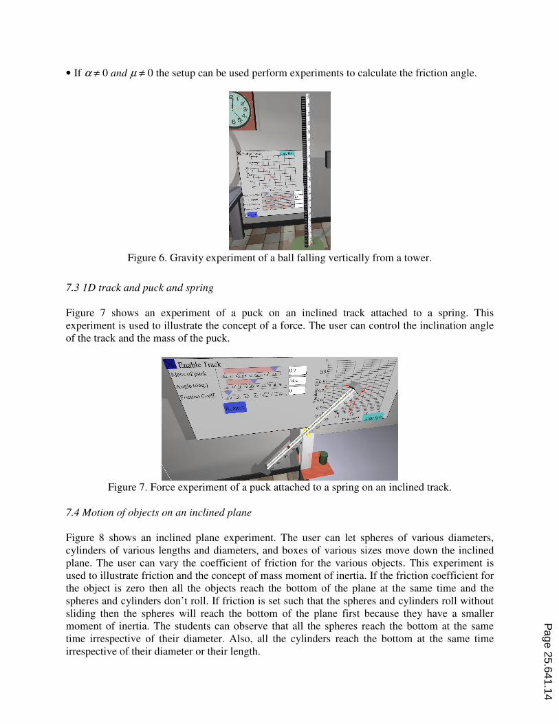
• If α ≠ 0 and µ ≠ 0 the setup can be used perform experiments to calculate the friction angle.

Figure 6. Gravity experiment of a ball falling vertically from a tower.

7.3 1D track and puck and spring

Figure 7 shows an experiment of a puck on an inclined track attached to a spring. This

experiment is used to illustrate the concept of a force. The user can control the inclination angle

of the track and the mass of the puck.

Figure 7. Force experiment of a puck attached to a spring on an inclined track.

7.4 Motion of objects on an inclined plane

Figure 8 shows an inclined plane experiment. The user can let spheres of various diameters,

cylinders of various lengths and diameters, and boxes of various sizes move down the inclined

plane. The user can vary the coefficient of friction for the various objects. This experiment is

used to illustrate friction and the concept of mass moment of inertia. If the friction coefficient for

the object is zero then all the objects reach the bottom of the plane at the same time and the

spheres and cylinders don’t roll. If friction is set such that the spheres and cylinders roll without

sliding then the spheres will reach the bottom of the plane first because they have a smaller

moment of inertia. The students can observe that all the spheres reach the bottom at the same

time irrespective of their diameter. Also, all the cylinders reach the bottom at the same time

irrespective of their diameter or their length.

Page 25.641.14

Figure 8. Inclined plane experiment showing various objects moving due to gravity on an

inclined plane.

7.5 Vertical Masses Rope-Pulley Experiment

Figure 1 shows two bodies suspended vertical using a rope and a pulley. The student can control

the values of the masses of the two bodies. The masses/inertia of the rope and pulley are

negligible compared to the masses of the suspended bodies. The motion of the bodies can be

used to derive Newton’s second law of motion. The rope is modeled using truss elements. The

contact search algorithm is used to quickly detect contact between the rope nodes and the pulley.

The rope and pulley are very light compared to the masses of bodies A and B in order not to

affect the results of the experiment.

7.6 Motion of a block on a frictional plane under the action of a force

Figure 9 shows a block on a plane connected to a vertical body using a rope and pulley. The

student can control the values of the masses of block and suspended body, the friction coefficient

and the contract area of the block. The experiment can be used to derive the Coulomb law for

friction. It can also be used to prove that the friction force is independent of the contract area.

Similar to the experiment in Figure 1, the rope and pulley are very light compared to the masses

of bodies A and B in order not to affect the results of the experiment.

Figure 9. Block on a frictional surface pulled by a mass using a rope and pulley used to illustrate

static friction.

Page 25.641.15

7.7 Motion of a puck on an inclined track under the action of a force

Figure 10 shows a puck on an inclined track connected to a vertical body using a rope and

pulley. The student can control the values of the masses of the puck and body, the inclination

angle of the track and the friction coefficient between the track the puck. The experiment can be

used to derive Newton’s second law and the Coulomb friction law.

Figure 10. Puck on an inclined track pulled by a mass using a rope and pulley.

7.8 Motion of a puck on circular track

Figure 11 shows a ball moving on a circular track. The student can control the initial angle of the

ball. This experiment is used to illustrate the concepts of periodic motion, kinetic energy,

potential energy and conservation of energy. The track is modeled using the inside surface of a

torus.

Figure 11. Puck moving on a circular track.

Page 25.641.16

7.9 Motion of a puck on roller-coaster track

Figure 12 shows a ball moving on a roller coaster track. The student can control the initial drop

height of the ball. The experiment is used to illustrate the concepts of kinetic energy, potential

energy, conservation of energy and conservation of momentum.

Figure 12. Puck moving on roller-coaster track.

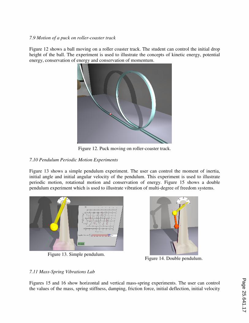
7.10 Pendulum Periodic Motion Experiments

Figure 13 shows a simple pendulum experiment. The user can control the moment of inertia,

initial angle and initial angular velocity of the pendulum. This experiment is used to illustrate

periodic motion, rotational motion and conservation of energy. Figure 15 shows a double

pendulum experiment which is used to illustrate vibration of multi-degree of freedom systems.

Figure 13. Simple pendulum.

Figure 14. Double pendulum.

7.11 Mass-Spring Vibrations Lab

Figures 15 and 16 show horizontal and vertical mass-spring experiments. The user can control

the values of the mass, spring stiffness, damping, friction force, initial deflection, initial velocity

Page 25.641.17

and applied force magnitude and frequency. Those experiments are used to illustrate the concepts

of simple harmonic motion, free undamped vibrations, free damped vibrations and forced

vibrations of one degree-of-freedom systems.

Figure 15. Horizontal mass-spring experiment. Figure 16. Vertical mass-spring experiment.

7.12 Spinning Top

Figure 17 shows a spinning top. The student can control moment of inertia of the top, the initial

angular velocity, the distance between the tip and the center of gravity (c.g.) and the offset of the

c.g. from the rotation axis of the top. The experiment is be used to illustrate gyroscopic motion.

Figure 17. Spinning top (for illustrating gyroscopic motion).

7.13 2D Air-Hockey Experiment

Figure 18 shows an air-hockey experiment. The experimental setup can be used to illustrate the

following concepts:

• Newton’s collision and momentum conservation laws for elastic and inelastic impacts.

• Newton’s first law of motion.

Page 25.641.18

Figure 18. Air-hockey experiment used to illustrate impact.

7.14 Billiards Table

Figure 19 shows a billiard table experiment. This experiment is also used to illustrate Newton’s

collision and momentum conservation laws.

Figure 19. Billiard table experiment.

7.15 Planetary Motion

Figure 20 shows a model of the solar system. The model includes the sun and all the planets. The

gravity forces between each pair of planets are included in model. The user can speed up time

and can turn-off/on some planets. The user can also control the initial position, velocity and mass

of an imaginary planet in order to see the different shapes of orbits. This experiment is used to

illustrate the concept of gravitational orbital motion.

Page 25.641.19

Figure 20. Solar system model.

7.16 String Vibrations

Figure 21 shows a vibrating string experiment. This experiment is used to illustrate the concepts

of transverse waves and vibration of continuous systems. The string is modeled using truss

elements under a pre-tension. The user can control the string pre-tension, axial stiffness and mass

per unit length. In addition, the user can set the initial conditions of the string in order to excite

the various modes of the string. Also, the user can pluck the string at one end and see a traveling

wave along the length of the string.

Figure 21. String vibration experiment.

Page 25.641.20

7.17 Gear Lab

The dynamics lab includes various gear trains including compound gear trains and planetary gear

trains (e.g. Figure 22). The student can observe the motion of the gears and observe the angular

velocity of the various gears as a function of the input angular velocity. For planetary gear trains

the input can be a sun gear, the arm or ring gear.

Figure 22. Gear lab.

7.18 Cam Lab

The dynamics lab includes four types of cam-follower systems (Figure 23):

• Cam with a translational flat face follower.

• Cam with a translational roller follower.

• Cam with an oscillating flat follower.

• Cam with a oscillating roller follower.

The student can specify the position diagram of the follower as a function of the cam angle, the

cam base radius and the follower radius. Then, the student can observe the motion of the cam

and follower and plot the velocity, acceleration and jerk diagrams for the cam.

Figure 23. Cams with: translating roller follow (left); translating flat follow (middle) and

oscillating flat follower (right).

Page 25.641.21

7.19 Robotic Manipulators

The dynamics lab includes a robotic manipulator (Figure 24). Students can specify the motion of

program the end effector from one point to another point in a straight line. Also, students can

specify the ending angles and positions of the various axes and observe the motion of the

manipulator. Students can plot the angles and the position of the end effector versus time.

Figure 24. Robotic manipulators.

7.20 Mechanism Lab

Figure 25, 26 and 27 show the user interface for specifying the dimensions of various types of

linkages including: 4-bar, crank-slider and inverted crank slider. The student can then animate

the motion of the linkage. They can plot the position of various points on the linkage. They can

also observe the motion of the mechanism under the action of applied torques and/or forces.

Figure 28 shows a typical 7-bar mechanism. Students can observe the motion of the mechanism

due to an applied torque and the presence of the spring.

Figure 25. 4-bar mechanism.

Page 25.641.22

Figure 26. Crank slider mechanism.

Figure 27. Inverted crank slider mechanism.

Figure 28. A 7-bar mechanism with a spring.

8. Concluding Remarks

A flexible multibody dynamics explicit time-integration parallel solver suitable for real-time

virtual-reality applications was presented. The multibody system includes rigid bodies, flexible

bodies, joints, frictional contact constraints, actuators and prescribed motion constraints. The

solver has the following characteristics/features:

Page 25.641.23

• Algorithm for accurate accounting for the rigid body rotational motion. The rigid bodies

rotational equations of motion are written in a body-fixed frame with the total rigid body

rotation matrix updated each time step using incremental rotations.

• Total-Lagrangian lumped parameters 3D finite elements including spring/truss and beam finite

elements.

• Penalty technique for modeling joint constraints including spherical, revolute, cylindrical and

prismatic joints.

• Penalty technique for modeling normal contact.

• Frictional contact modeled using an accurate and efficient asperity-based friction model.

• General fast hierarchical bounding box-bounding sphere contact search algorithm for finding

the contact penetration between points on master contact surfaces and polygons on slave

contact surfaces.

• Hierarchical object-oriented framework. The hierarchical “scene-graph” representation of the

model used for display and user-interaction with the model is also used in the solver.

The application of the real-time solver to a virtual dynamics lab was presented.

References

1. Wasfy, T.M. and Noor, A.K., “Computational strategies for flexible multibody systems,” ASME Applied

Mechanics Reviews, Vol. 56(6), pp. 553-613, 2003.

2. Uchida T. and McPhee, J., “Triangularizing kinematic constraint equations using Gröbner bases for real-time

dynamic simulation,” 1st Joint International Conference on Multibody System Dynamics, Lappeenranta,

Finland, May 2010.

3. Hidalgo, A., Callejo, A., and de Jalon, J.G., “Using implicit integrators and automatic differentiation to compute

large and complex MBS in real-time,” 1st Joint International Conference on Multibody System Dynamics,

Lappeenranta, Finland, May 2010.

4. Lugris, U., Escalona, J., Dopico, D. and Cuadrado, J, “Efficient and accurate simulation of the cable-pulley

interaction in weight-lifting machines,” 1st Joint International Conference on Multibody System Dynamics,

Lappeenranta, Finland, May 2010.

5. Cuadrado, J., Dopico, D., Gonzalez, M. and Naya, M.A., “A combined penalty and recursive real-time

formulation for multibody dynamics,” Journal of Mechanical Design, Vol. 126(4), 2004, pp. 602-609.

6. Perera H.S. and Romano, R. and Nunez, P., “Automated methods for converting a non real-time Cartesian

multi-body vehicle dynamics model to a real-time recursive model,” SAE International 2006 World Congress,

Detroit, Michigan, April, 2006.

7. Heyn, T. Mazhar, h., Tasora, A, Negrut, D., “Tracked vehicle simulation on granular terrain leveraging parallel

computing on GPUs,” 1st Joint International Conference on Multibody System Dynamics, Lappeenranta,

Finland, May 2010.

8. Hippmann, G., “An algorithm for compliant contact between complexly shaped surfaces in multibody

dynamics,” IDMEC/IST, Lisbon, Portugal, July 2003.

9. Wasfy, T.M. and Noor, A.K., “Modeling and sensitivity analysis of multibody systems using new solid, shell

and beam elements,” Computer Methods in Applied Mechanics and Engineering, Vol. 138(1-4) (25th

Anniversary Issue), pp. 187-211, 1996.

10. Wasfy, T.M., “Modeling spatial rigid multibody systems using an explicit-time integration finite element solver

and a penalty formulation,” ASME Paper No. DETC2004-57352, Proceeding of the DETC: 28th

Biennial

Mechanisms and Robotics Conference, DETC, Salt Lake, Utah, 2004.

11. Wasfy, T.M., “A torsional spring-like beam element for the dynamic analysis of flexible multibody systems,”

International Journal for Numerical Methods in Engineering, Vol. 39(7), pp. 1079-1096, 1996.

Page 25.641.24

12. Wasfy, T.M. and O’Kins, J., “Finite Element Modeling of the Dynamic Response of Tracked Vehicles,” 7th

International Conference on Multibody Systems, Nonlinear Dynamics, and Control, San Diego, CA, August

2009.

13. Wasfy, T.M., “High-fidelity modeling of flexible timing belts using an explicit finite element code,” ASME

DETC2011-48846, Proceedings of the ASME 2011 International Design Engineering Technical Conferences &

Computers and Information in Engineering Conference (IDETC/CIE 2011), 8th

International Conference on

Multibody Systems, Nonlinear Dynamics, and Control, Washington, DC, August 2011.

14. Wasfy, T.M., Wasfy, H.M, and Peters, J.M., “Real-time explicit flexible multibody dynamics solver with

application to virtual-reality based e-learning,” ASME DETC2011-48846, Proceedings of the ASME 2011

International Design Engineering Technical Conferences & Computers and Information in Engineering

Conference (IDETC/CIE 2011), 8th

International Conference on Multibody Systems, Nonlinear Dynamics, and

Control, Washington, DC, August 2011.

15. Leamy, M.J. and Wasfy, T.M., “Transient and steady-state dynamic finite element modeling of belt-drives,”

ASME Journal of Dynamics Systems, Measurement, and Control, Vol. 124(4), pp. 575-581, 2002.

16. Wasfy, T.M. and Leamy, M.J., “Modeling the dynamic frictional contact of tires using an explicit finite element

code,” ASME DETC2005-84694, 5th

International Conference on Multibody Systems, Nonlinear Dynamics,

and Control, Long Beach, CA, September 2005.

17. Wasfy, T.M., “Asperity spring friction model with application to belt-drives,” Paper No. DETC2003-48343,

Proceeding of the DETC: 19th

Biennial Conference on Mechanical Vibration and Noise, Chicago, IL, 2003.

18. Wasfy, T.M. and Noor, A.K., “Object-oriented virtual reality environment for visualization of flexible

multibody systems,” Advances in Engineering Software, Vol. 32(4), pp. 295-315, March 2001.

19. Wasfy, T.M. and Leamy, M.J., “An object-oriented graphical interface for dynamic finite element modeling of

belt-drives,” 27th

Biennial Mechanisms and Robotics Conference, ASME International 2002 DETC, Montreal,

Canada, 2002.

20. Wasfy, T.M. and Wasfy, A.M., “An object-oriented graphical interface for dynamic finite element modeling of

flexible multibody mechanical systems,” Proceeding of MDP-8, Cairo University Conference on Mechanical

Design and Production, Cairo, Egypt, January 4-6, 2004.

21. Wasfy, T.M., “Object-oriented modeling environment for simulating flexible multibody systems and liquid-

sloshing,” DETC2006-99245, 26th

Computers and Information in Engineering (CIE) Conference, ASME

DETC, Philadelphia, PA, September 2006.

22. Wasfy, T.M. and Wasfy, H.M., “Object-oriented environment for dynamic finite element modeling of tires and

suspension systems,” IMECE2006-13848, 2006 Mechanical Engineering Congress and Exposition Conference,

Chicago, IL, November 5-10, 2006.

Page 25.641.25