Academic year 2007

Computing projectGroup report

SBML-ABC, a package for data simulation,parameter inference and model selection

Imperial College- Division of Molecular Bioscience

MSc. Bioinformatics

Nathan Harmston, David Knowles, Sarah Langley, Hang Phan

Supervisor:

Professor Michael Stumpf

June 13, 2008

Contents

1 Introduction 11.1 Background. . . . . . . . . . . . . . . . . . . . . . . . . . . . . . . . . . . . . . 1

2 Features and dependencies 22.1 Project outline. . . . . . . . . . . . . . . . . . . . . . . . . . . . . . . . . . . . . 22.2 Key features. . . . . . . . . . . . . . . . . . . . . . . . . . . . . . . . . . . . . . 2

2.2.1 SBML. . . . . . . . . . . . . . . . . . . . . . . . . . . . . . . . . . . . . 22.2.2 Stochastic simulation. . . . . . . . . . . . . . . . . . . . . . . . . . . . . 42.2.3 Deterministic simulation. . . . . . . . . . . . . . . . . . . . . . . . . . . 42.2.4 ABC inference. . . . . . . . . . . . . . . . . . . . . . . . . . . . . . . . 5

2.3 Interfaces . . . . . . . . . . . . . . . . . . . . . . . . . . . . . . . . . . . . . . . 52.3.1 C API . . . . . . . . . . . . . . . . . . . . . . . . . . . . . . . . . . . . . 52.3.2 Command line interface. . . . . . . . . . . . . . . . . . . . . . . . . . . 52.3.3 Python . . . . . . . . . . . . . . . . . . . . . . . . . . . . . . . . . . . . 52.3.4 R . . . . . . . . . . . . . . . . . . . . . . . . . . . . . . . . . . . . . . . 6

2.4 Dependencies. . . . . . . . . . . . . . . . . . . . . . . . . . . . . . . . . . . . . 6

3 Methods 83.1 SBML Adaptor . . . . . . . . . . . . . . . . . . . . . . . . . . . . . . . . . . . . 83.2 Stochastic simulation. . . . . . . . . . . . . . . . . . . . . . . . . . . . . . . . . 8

3.2.1 Random number generator. . . . . . . . . . . . . . . . . . . . . . . . . . 93.2.2 Multicompartmental Gillespie algorithm. . . . . . . . . . . . . . . . . . . 93.2.3 Tau leaping. . . . . . . . . . . . . . . . . . . . . . . . . . . . . . . . . . 103.2.4 Chemical Langevin Equation. . . . . . . . . . . . . . . . . . . . . . . . . 11

3.3 Deterministic algorithms. . . . . . . . . . . . . . . . . . . . . . . . . . . . . . . 113.3.1 ODE solvers . . . . . . . . . . . . . . . . . . . . . . . . . . . . . . . . . 113.3.2 Time Delay Differential Equation solver. . . . . . . . . . . . . . . . . . . 11

3.4 Parameter inference. . . . . . . . . . . . . . . . . . . . . . . . . . . . . . . . . . 123.4.1 ABC rejection . . . . . . . . . . . . . . . . . . . . . . . . . . . . . . . . 123.4.2 ABC MCMC . . . . . . . . . . . . . . . . . . . . . . . . . . . . . . . . . 123.4.3 ABC SMC parameter inference. . . . . . . . . . . . . . . . . . . . . . . 12

3.5 ABC SMC model selection. . . . . . . . . . . . . . . . . . . . . . . . . . . . . . 133.6 Interfaces . . . . . . . . . . . . . . . . . . . . . . . . . . . . . . . . . . . . . . . 14

3.6.1 Command line interface. . . . . . . . . . . . . . . . . . . . . . . . . . . 143.6.2 C API . . . . . . . . . . . . . . . . . . . . . . . . . . . . . . . . . . . . . 14

i

3.6.3 Python - C Binding. . . . . . . . . . . . . . . . . . . . . . . . . . . . . . 153.6.4 R interface . . . . . . . . . . . . . . . . . . . . . . . . . . . . . . . . . . 16

4 Examples and results 194.1 Data simulation. . . . . . . . . . . . . . . . . . . . . . . . . . . . . . . . . . . . 19

4.1.1 Lotka-Volterra model. . . . . . . . . . . . . . . . . . . . . . . . . . . . . 194.1.2 Repressilator. . . . . . . . . . . . . . . . . . . . . . . . . . . . . . . . . 204.1.3 Brusselator model. . . . . . . . . . . . . . . . . . . . . . . . . . . . . . 20

4.2 Parameter inference. . . . . . . . . . . . . . . . . . . . . . . . . . . . . . . . . . 214.2.1 ABC rejection . . . . . . . . . . . . . . . . . . . . . . . . . . . . . . . . 214.2.2 ABC MCMC . . . . . . . . . . . . . . . . . . . . . . . . . . . . . . . . . 214.2.3 ABC SMC . . . . . . . . . . . . . . . . . . . . . . . . . . . . . . . . . . 25

4.3 Model selection. . . . . . . . . . . . . . . . . . . . . . . . . . . . . . . . . . . . 25

5 Future work 28

ii

List of Figures

2.1 Flowchart of SBML-ABC package. . . . . . . . . . . . . . . . . . . . . . . . . . 3

3.1 Screen shot of instruction on how to use the the programsbmlabc . . . . . . . . . 18

4.1 Lotka-Volterra simulated using Gillespie’s algorithm. . . . . . . . . . . . . . . . . 194.2 Repressilator simulated using ODE solver.. . . . . . . . . . . . . . . . . . . . . . 204.3 Feedback loops present in repressilator. . . . . . . . . . . . . . . . . . . . . . . . 204.4 Simulations of the Brusselator model using different algorithms. . . . . . . . . . . 224.5 Results of ABC rejection on Brusselator model using ODE solver. . . . . . . . . . 234.6 Observed data (blue) and accepted simulated data (gray lines). . . . . . . . . . . . 234.7 Results of ABC MCMC on Brusselator model using ODE solver. . . . . . . . . . . 244.8 Histograms of log(distance) for all simulated datasets. . . . . . . . . . . . . . . . . 244.9 Parameter 1 vs. 4 from ABC SMC with 8 populations, 1000 particles on Brusse-

lator using ODE solver. Populations are shown added two per plot. . . . . . . . . . 264.10 Acceptance ratio againstǫ for each population of ABC SMC.. . . . . . . . . . . . 27

iii

Chapter 1

Introduction

We present a computational package for the simulation of dynamical systems and the inference ofparameters in these models based on experimental time course data. Models are imported usingthe Systems Biology Markup Language (SBML) [1] and simulated using a range of determin-istic and stochastic algorithms. The main contribution of this project however is to provide anaccessible package to infer feasible model parameters using Approximate Bayesian Computationmethods [2], including ABC rejection, Markov Chain Monte Carlo, and Sequential Monte Carlo.

1.1 Background

Several packages exist to search the parameter space of a dynamical model to find the “optimum”values. The complex pathway simulator Copasi [3], has a range of stochastic optimisation methodswhich use steady state or time course experimental data and deterministic or stochastic simulations.COPASI supports import of Systems Biology Markup Language (SBML) [1] models and providesthe choice of a command line, graphical user interface or C Application Programming Interface(API). SBML-PET [4] is an alternative package which performs stochastic ranking evolutionarysearch (SRES) [5] based on the ODEPACK [6] solver LSODAR. A key advantage of this packageis its ability to handle SBML events.

The key flaw with existing packages is the lack of any consideration of the range of feasibleparameters. In a Bayesian framework we would ideally like todo this by calculating the poste-rior over the parameters given the observed data. Since we cannot directly evaluate the likelihoodfunction in complex biological models, we employ the Approximate Bayesian Computation frame-work [2] where we compare data simulated using various parameter values to observed data. Thisframework provides a theoretical foundation which is lacking from existing methods, where themeaning of “best parameters” is ill-defined. The samples found can provide insight into the modelbehaviour and give confidence intervals for each parameter.

1

Chapter 2

Features and dependencies

In this chapter, we introduce the project, in terms of the keyfeatures, the four interfaces, anddependencies on specific packages and platforms.

2.1 Project outline

In order to provide a complete package for model inference, we implemented a three-faceted soft-ware package, consisting of modules for SBML parsing, stochastic and deterministic data simu-lation, and ABC inference. A schematic of the components is shown in Figure2.1. Four distinctinterfaces are available: a command line executable, a C API, and R and Python interfaces, pro-viding options for users of any level of computing knowledge.

2.2 Key features

2.2.1 SBML

SBML is an xml-based markup language specifically designed to aid the “exchange and re-use ofquantitative models” [1]. It is designed to be both computer and human readable and a numberof packages exist which are able to take a model defined in an SBML file and perform simula-tion or other algorithms on the model.LibSBML [7] is a library designed specifically for read-ing, writing and modifying SBML models. This library is written in C and C++, although ithas bindings available for a number of languages including,Python, Java, Perl and Ruby. It isdesigned to be portable and it has been ported to many different platforms including, Windows,Linux and Mac OS X. Many researchers have made the models theyhave produced freely availableatwww.biomodels.org, leading to a growing corpus of models for examination and testing ofbiological simulators. The models encoded within SBML can be extremely complex and SBMLsupports encoding of both stochastic and deterministic models. It is possible to encode not onlycellular models within SBML but also population genetics models, although not many of thistype are currently in use. There are many competitors to the SBML format including BioPAXand CellML, although BioPAX is primarily for the encoding ofbiological pathways rather thanbiological models.

2

SBML model(s)

libSBML

SBML adaptor

Gillespie

struct

ODE struct &

gradient

function

DDE struct &

gradient

function

ABC

rejection, MCMC, SMC or MS

Gillespie GSL/CVODE ddesolve

Observed data

Model

representation

Simulation

algorithms

Parameter samples

CLE struct &

propensity

function

CLE/tau leap

Figure 2.1: Flowchart of SBML-ABC package

Our software package supports the importing of biological models written in SBML and theability to simulate these models either stochastically or deterministically and perform parameterinference on these models. The SBML-ABC package supports a subset of the current SBMLspecification. The main components of the specification are supported including reactions, com-partments, species, parameters, kinetic laws and rate laws(differential equations). Currently thepackage only supports inference on global parameters and all parameters declared locally to a re-action will be used with the value as set within the list of parameters local to that kinetic law.Currently the simulation algorithms for CLE, DDE and ODE allcan make use of generated sharedlibraries to enable faster running times of these algorithms. The generated libraries contain either afunction containing the differential equations corresponding to each species or a representation ofthe kinetic law. The differential equations can either be generated using the kinetic laws which areset for each reaction or have a rate rule set for the species. In the case where kinetic laws are notdefined for a model, the SBML adaptor will automatically generate a file containing the standard

3

mass action kinetic laws for the model. This process is not seen by the user. This auto-generationof the gradient function is only supported for ODE simulation algorithms. In the case of a userwanting to run a Gillespie simulation on a SBML model, the SBML file must be written with eachof the global parameters corresponding to the reaction rateof a reaction, for example the rate ofthe first reaction in the SBML file should be encoded as the firstglobal parameter.

A significant subset of MathML in the SBML specification is supported: all of the main arith-metic operations and trigonometric functions are implemented have been tested. However, logicaland relational operations and custom function definitions are not supported.

2.2.2 Stochastic simulation

There are two analytical approaches to modeling biochemical systems: deterministic and stochas-tic. Deterministic methods are used when a system can be defined while neglecting random effectsand species can viewed as continuous without drastically distorting the behavior of the system.Systems of ordinary and time-delay differential equationscan then model the system to an accept-able accuracy. Stochastic methods describe systems where species are defined in discrete termsand failing to consider random effects can cause simulations to differ from observed results.

Stochastic simulation plays an important part in the understanding of biochemical systems ofreactions including gene regulation networks, metabolic networks, and reaction systems where thedeterministic approach is not suitable because very low particle numbers make stochastic effectssignificant.

The foundation of the stochastic simulation of biochemicalsystem is the Gillespie Stochas-tic Simulation Algorithm (SSA) [8, 9] which is “exact” given some basic physical assumptions,such as having a ”well-mixed” system. Stochastic algorithms have seen significant improvementsin speed during the past three decades allowing the simulation of more complex systems. No-table algorithms are the Gibson & Bruck’s next reaction method [10], chemical Langevin equation(CLE) [11], and tau leaping methods [12, 13, 14]. As the biological systems are complex, and it isvital to understand it closer to its natural form, a new computing system has been developed, theP-system [15] in 2000 by Paun Gh., abstracting the way the alive cells manipulate chemical sub-stances in multi compartmental situations. The original Gillespie’s algorithm has been extended tosimulate the behaviour of transmembrane P-systems, introduced as the multicompartmental Gille-spie algorithm [16] where the movement of crossing the membrane from one compartment to theother is taken into account.

Three simulation algorithms are implemented in our project: tau leaping, the CLE method andthe multicompartmental Gillespie algorithm (which is the SSA when the number of compartmentsis 1). The SSA, tau leaping and CLE method are widely available in many packages but the mul-ticompartmental algorithm is not yet commonly used. The SSAis not implemented separately asthe multicompartmental Gillespie algorithm reduces to theSSA when it is a single compartmentalsystem.

2.2.3 Deterministic simulation

The Chemical Langevin Equation is equivalent to the Euler-Maruyama scheme for the numeri-cal integration of stochastic differential equations (SDE), when applied to the chemical masterequation. The system is therefore implicitly being represented as an SDE, which motivates the

4

approximation of such a system by a system of deterministic equations, i.e. ordinary differentialequations (ODEs). Deterministic simulations have the advantage of being much faster than theirstochastic counterparts, and the literature on the numerical integration of ODEs is very well devel-oped. Runge-Kutta schemes are thede factosolution, and coupled with adaptive step size control,which ensures the local error remains below a user specified tolerance, they provide a powerfultool for rapid data simulation in situations where particlenumbers are sufficiently large to allowus to ignore stochastic effects. Runge-Kutta-Fehlberg 45 is the default solver in our package, butmore advanced solvers are availablse through the GSL and CVODE which can handle stiff sets ofequations where differential components of the system operate on very diverse time scales.

2.2.4 ABC inference

This project is complementary to work by Toni et al. developing the ABC Sequential Monte Carlofor parameter inference and model selection [17]. The basic concept in Approximate BayesianComputation is to repeatedly draw parameter samples from their prior and simulate data under themodel of interest using these parameter samples. If the datasimulated with a particular parametervector is sufficiently similar to observed data on some choice of distance measure, then we acceptthe sample as being from the approximate posteriorP (θ|ρ(x, x∗) ≤ ǫ), wherex is observed data,x∗ is the simulated data,ρ is the distance function andǫ is the threshold for acceptance. The choiceof ǫ is crucial. Too small, and the acceptance ratio will be unacceptable small, too large and theapproximate will be very poor.

For computationally intensive algorithms, such as ABC SMC parameter inference and modelselection, it is of great value to be able to recover and resume a simulation if it is stopped. Wehave designed the ABC SMC methods to retrive the previous population of samples particles andcontinue the algorithm from that population. This is also a useful feature if one wants to alter theparameter settings for future populations.

2.3 Interfaces

2.3.1 C API

The C API provides the most flexible interface to the package.It is the only interface through whicharbitrary parameter assignment functions can be used, allowing specific subsets of parameters orparameters such as the initial conditions to be inferred. Italso allows straightforward integrationof new simulation algorithms.

2.3.2 Command line interface

The command line interface is very user friendly, using flagsand defined input files to control theoperation. The full range of simulation and inference algorithms are available.

2.3.3 Python

Python is a multi-paradigm scripting language which is widely used in both academia and indus-try. It is a dynamic, strongly typed object-oriented programming language. Python has features

5

which support both aspect-oriented and functional programming as well as imperative and object-oriented programming styles. Most programmers regard Python as an very productive language toprogram in due to its concise syntax and uses indentation to define code blocks. This syntax forcesprogrammers to write code that is easier to read and makes python code extremely maintainableand easily extendable. Python has automatic garbage collection based on reference counting andcycle detection and as such it reduces the programming time associated with dealing with memoryrelated issues. Python also comes with an extensive standard library which as of Python 2.5 in-cludes ctypes and a BioPython package [18] is also freely available which contains code useful tothe bioinformatics community. Python is freely available and released under an OSI approved opensource license. Python is very popular with researchers from a Physics, maths or computer sci-ence background and is gaining popularity in the bioinformatics and systems biology community.There are several implementations of the Python specification available including Jython (based onJava), IronPython (based on .NET) and CPython (based on C) which is the most commonly usedimplementation. Although there should be no major problemswith portability between differentPython implementations, this package has only been tested using CPython.

A number of different methods exist for integrating Python with C code such as Weave, SWIGand ctypes. Ctypes is a foreign function interface which supports accessing methods and variableslocated in a shared library and allows a Python programmer toaccess these almost transparentlywithout the need to write any bespoke C code. This reduces thedevelopment time in interfacing Cand Python code.

2.3.4 R

The freely available statistics programming environment R[19] is used greatly within the bio-logical community, and so creating an interface between R and the above Approximate BaysianComputation (ABC) methods, differential equation solversand SBML parser was an obvious. Alimited SBML parser and simulation package exists [20] and is available in the BioConductordownloadwww.bioconductor.org. However, this package is limited in the variety of SBMLfiles it is able to parse and is only able to call the existing odesolve() function in R to simulate themodel.

R has a vast amount of external packages pertaining to the biological sciences as well as pro-tocol for writing new packages. It has the ability to seamlessly integreate several packages anddata files into one workspace and provides a publication-worthy base graphics package. Data ma-nipulation in R depends on vector, matrix and list structures, which makes it ideal for representingthe data structures needed and produced by our package. The Rimplementation is currently im-plemented and supported on Linux and MacOS, and will become available on Windows in thefuture.

2.4 Dependencies

GNU Scientific Library. SBML-ABC makes extensive use of the GNU Scientific Library (GSL).We use the implementation of the Mersenne twister random number generator from GSL to gen-erate the random numbers used in the simulations and uses thegsl matrix andgsl vectordata structures for large portions of handling options and data handling. We provide support for

6

using the ode solving algorithms found in GSL. The package has been tested with version 1.11 ofthe GSL.

libSBML. The package is dependent on the libSBML library, which is available fromhttp://www.sbml.org/Software/libSBML and provides the functionality to read, write andmanipulate SBML files. LibSBML is used to extracts the model encoded in an SBML file and thenbuilds an internal representation of the model, which is a more efficient representation and reducesthe time and space requirements for the simulation algorithms.

gcc. The GNU Compiler Collection (gcc) is used to compile the gradient and propensity func-tions derived from the SBML files. The package has been testedwith gcc4.3.1.

Python. The Python modules included in this package require Python 2.5 or later due to the needfor ctypes and the use of language features only available inPython 2.5.

R. The R package derived from the C code was built and tested under R 2.5.

Platform. The package has been tested on Linux and Mac OSX and has not been tested on aWindows platform and there will be difficulties in compilingand loading the generated sharedlibraries used for the gradient and propensity functions.

7

Chapter 3

Methods

In this chapter, we describe in detail the method provided inthe package. The core algorithmsare implemented in C, including the SBML adaptors, the deterministic and stochastic simulators,ABC parameter inference and model selection algorithms. Finally the interfaces and their usagewill be described.

3.1 SBML Adaptor

Although the SBML format is a good way of encoding models it isan extremely inefficient rep-resentation for use by simulation algorithms. A C module wascreated which made it possible toimport an SBML model and build a representation of the model which we designed for use in thesimulation algorithms. The module was designed to be as modular as possible in order to minimisecode redundancy and decrease development time. The conversion code makes extensive use of thelibSBML library which is designed to allow the manipulationof SBML models. The SBML adap-tor code supports the generation of shared libraries containing gradient and propensity functionsfor use in the ODE, DDE and CLE simulation algorithms. This was done to reduce the executiontime of the simulation algorithms and increase the flexibility of the algorithms.

3.2 Stochastic simulation

A biochemical system in stochastic simulation scheme is defined as a well stirred system ofNspecies{S1, S2, ..., SN} andM reactions{R1, R2, ..., RM} with relative ratesc1, c2, ...cM . Xi(t)the number of speciesSi in the system at timet. The stochastic simulation problem is to estimatethe state vectorX(t) ≡ (X1(t), X2(t), ...XN(t)) given the initial state vectorX(t0) = x0 at initialtime t0.

The propensity functionhi(t) of a reaction, e.g. the probability a reaction takes place inthesystem, depends on the availability of the species requiredfor the reaction and the reaction rate. Itis a function proportional to the combinatory of number of species available and the reaction rate.For example, a first degree reactionR1(c1) : X → Y has a propensityh1(t) = c1 × [X](t), and asecond degree reactionR2(c2) : X + Y → 2X has the propensityh2(t) = c2 × [X](t)[Y ](t).

8

3.2.1 Random number generator

An important issue in stochastic simulation problem is the random number generation(RNG) toobtain the random factor in the simulation process, e.g. computing the time until the next reac-tion and choosing the next reaction. It is also useful in other parts of the project, i.e., the ABCMCMC, ABC SMC algorithms where the Monte Carlo process requires the RNG. Random num-bers generated by any computational algorithms are only pseudo-random number. A good randomnumber generator is the one that satisfies both theoretical and statistical properties, which are hardto obtain.

In our project, we use the random number generators providedby GSL (GNU Scientific Li-brary,http://www.gnu.org/software/gsl/manual/), thegsl rng. gsl rng is aclass of generators that generate random number from different distributions, such as uniform,normal, and exponential, and are convenient to use. The coreof the generators we use is thedefault generatormt19937, the portable Mersenne Twister random number generator. Inthestochastic simulation scheme, only sampling from a uniformdistribution is required. However, inthe ABC scheme, Gaussian distribution sampling and others are necessary to extend the variety ofthe algorithms.

3.2.2 Multicompartmental Gillespie algorithm

Gillespie’s algorithm ( [8], [9]), or stochastic simulation algorithm (SSA) is an exact method forthe stochastic simulation of biochemical system of reactions described above. It stochasticallysimulates the system depending mainly on the propensity of reactions in the system by taking intoaccount the random factor to the next reaction to occur and the time until the next reaction occurs.There are two Gillespie’s algorithms, the direct method andthe first reaction method, which areequivalent in terms of statistic. However, the direct method is faster and simpler to implement thanthe other, thus it is more commonly used.

Since the development of the SSA, several improvements havebeen made to improve or extendit. Gibson & Bruck’s next reaction method [10], tau-leaping [12, 13, 14] and chemical Langevinequation (CLE) method [11] speed up the stochastic simulation by adapting a certain time intervalfor the system to proceed. Another direction in further improvement of the SSA has been made byextending it to the P-system [15], a computing model abstracting from the compartmental structureof alive cells in processing chemicals. The P-system is capable of describing the behaviour ofa biologically meaningful system. A stochastic simulationmethod has been introduced for thissystem to simulate the kinetics of species in the multicompartment system based on the SSA,which we will refer to as the multicompartmental Gillespie algorithm [16]. The key idea of themulticompartmental Gillespie algorithm is to decide the compartment where the next reactionoccurs, by computing theτ andµ value for each compartment, and then choosing the one with thesmallestτ .

In our project, we implement the multicompartmental Gillespie algorithm. However, as thesimulation framework is designed to fit the main overall targets of the project which are the ABCscheme for parameter approximation, it is required that thesystem is simple enough to comparemodels. Thus, the system in our implemented version (see Algorithm 1) is reduced to a simplersystem compared with the P-system. The same type of species in different compartments are de-fined in the SBML file with different species name and thus species ID, thus when it moves from

9

one compartment to another, it is not considered a diffusionof chemical substances as described inthe paper [16]. Furthermore, this simplified version ignores the “environment” element and it doesnot use a heap sort for the triple (τi, µi, i) wherei is the compartment index, but performs a min-imum finding every loop. This version of the multicompartmental Gillespie simulation becomesthe original Gillespie’s algorithm when the number of compartments is 1.

Algorithm 1 Multicompartmental Gillespie’s algorithm1: INPUT: Time series (t0, t1, ..., tN )of simulated data, model of simulation2: OUTPUT: System states at desired time points3: Initialize the timet = t0, system’s statex = x0

4: Calculate reaction propensity functionsaj(x) andai0(x =

∑rj∈Ci

j aj(x))

5: Calculateτi = 1ai0

ln(rand(0, 1))

6: Calculateµi:∑µi−1,rj∈Ci

j=0 aj < rand(0, 1)ai0 <

∑µi,rjinCi

j=0 aj (j is the index of reactions in thecompartment only)

7: Seti = 08: repeat9: GetCi whereτi is smallest

10: Execute reactionµi of compartmentCi, update the system’s state:t → t + τ , x → x + νµ.11: Recalculate reaction propensity functionsaj(x) andai

0(x =∑

j aj(x)) of reactions affectedby rµj

12: Recalculateτi = 1a0

ln(rand(0, 1)) of compartments affected byrµj

13: Recalculateµi:∑µi−1,rj∈Ci

j=0 aj < rand(0, 1)ai0 <

∑µi,rjinCi

j=0 aj of comparments affected byrµi

(j is the index of reactions in the compartment only)14: if t = ti then15: recordx(t)16: incrementi17: end if18: until End condition

The multicompartmental Gillespie algorithm use a data structure close to the model descriptionin SBML, theStochasticModel comprising of Compartment information, Compartment (witha pointer to the Compartment information), Species information, Species (with a pointer to theSpecies information), Reaction (containing Species type Reactants, Modifers and Products andreaction rate). This data structure enables the algorithm to work in an efficient interlinked mannerthat helps avoiding random errors. The structure include a pointer to a random number generatorto be activated everytime the model is parse from the SBML file. It also has a block of structuresto increase the speed of updating the system status by storing the reactions being affected by theexecution of a reaction (similar to the idea of dependency graph notion introduced in the Nextreaction method [10]).

3.2.3 Tau leaping

Tau leaping is an approximation to the exact Gillespie algorithm. Consider all the reactions in atime interval[t, t + τ ]. Denote the number of times reactionj occurrs asPj . If the time interval

10

is short enough the propensity functionsaj(·) will not change much over this interval. Indeed, ifwe assumeaj(·) has the value at the beginning of the interval over the whole interval, then eachPj will have Poisson distribution with expected valueaj(X(t))τ . Once we have thePj ’s, we applythe equation:

X(t + τ) = X(t) +

M∑

j=1

νjPj(aj(X(t)), τ) (3.1)

whereνj is the stoichiometry of thejth reaction. Tau leaping is analogous to the simple forwardEuler method for simulating ODEs, and suffers from the same numerical instability. More ad-vanced alternatives such as implicit tau leap are outside the scope of this project, but would be aninteresting avenue for further investigation. Tau leap uses theCLEModel settings structure.

3.2.4 Chemical Langevin Equation

The tau leap algorithm can also be seen as a stepping stone to the Chemical Langevin Equation(CLE), a Stochastic Differential Equation (SDE) that approximates the solution further. Recall thatthe amount each reaction occurs in the interval[t, t + τ ], denotedPj, is Poisson distributed withmeanλ = aj(X(t))τ . It is a basic result from probability theory that for large counts, a Poissonrandom variable is well approximated by a normal variable with mean and variance both equal toλ. In applying this approximation our state variables becomecontinuous rather than discrete, andwe arrive at the CLE:

X(t + τ) = X(t) + τ

M∑

j=1

νjaj(X(t)) +√

τ

M∑

j=1

νj

√

aj(X(t))Zj (3.2)

whereZj are unit normal random variables.

3.3 Deterministic algorithms

3.3.1 ODE solvers

For simulating ODEs both the full range of solvers in the GSL and a subset of the CVODE solversare available. GSL solvers are used viaodesolve whereas CVODE solvers are accessed viacvodesolve. The default GSL solver is Runge Kutta Fehlberg 4-5, where the gradient eval-uations for a 5th order Runge Kutta (RK) step are used to take a4th order step ”for free”. Thecomparison between these two steps allows an estimate of theerror, and hence facilitates errorcontrol. For stiff problems the implicit GEAR 1 and 2 methodsare available. If a Jacobian is avail-able the Burlish-Stoer implicit method should be used. The default CVODE solver is the BackwardDifferentiation Formula, with Newton iterations to solve the resulting fixed point problem.

3.3.2 Time Delay Differential Equation solver

The time delay differential equation (DDE) solver code is based on the R packageddesolvewhich is turned based onsolv95. The core is an embedded RK 23 step and cubic Hermitian

11

interpolation to calculate lagged variables between simulated time points. Various modificationsand simplifications have been made, including moving to an object orientated framework to makedynamically loading a compiled gradient function possible. Although switch functions are notused their associated code has not been removed since they would be useful if SBML events wereincorporated in the future.

3.4 Parameter inference

3.4.1 ABC rejection

Approximate Bayesian Computation(ABC) allows us to infer the parameters of a system in prob-lems where we cannot evaluate the likelihood functionf(x|θ) but can draw samples from it bysimulating the system. The simplest algorithm is ABC rejection [21], as described in Algorithm2.ABC rejection is implemented by constructing anABCRejectionSettings structure and call-ing abcRejection. For more details please refer to the C API User Guide in the Appendix.

Algorithm 2 ABC rejection. x0 denotes observed data.ρ(·) denotes a distance measure.ǫ is athreshold set by the user.

repeatSampleθ∗ from the priorπ(θ)Simulatex∗ as a sample fromf(x|θ∗)Acceptθ∗ if ρ(x∗, x0) ≤ ǫ

until enough samples found

3.4.2 ABC MCMC

ABC rejection is inefficient because it will continue to drawsamples in regions of parameter spacethat are clearly not useful. One approach to this problem is to derive a ABC Markov Chain MonteCarlo (MCMC) algorithm [2], as specified in Algorithm3. The hope is that the Markov chain(MC) will spend more time in interesting regions of high probability compared to ABC rejection.However, strongly correlated samples and low acceptance ratios means that ABC MCMC can infact be highly inefficient, especially if the MC gets stuck ina region of low probability for a longtime, requiring a significant burn in period.

3.4.3 ABC SMC parameter inference

ABC MCMC has a potential disadvantage being inefficient, being stuck in a regions of low accep-tance probability for a long time due to the correlated nature of samples and thus more computa-tionally intensive. This problem can be tackled by using another approach, the ABC SequentialMonte Carlo (SMC) methods [22], which introduces a sequence of intermediate distributions. Thisapproach has been adapted with the sequential importance sampling algorithm [23, 24] and intro-duced in a paper to be published by Tina Toni [17]. In our project, we implement the algorithmsdescribed in this paper, the weighted ABC SMC algorithm4 where the samples are derived from

12

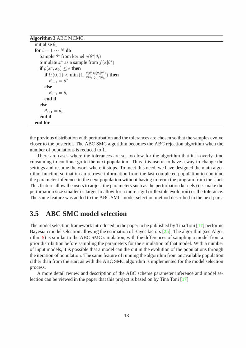
Algorithm 3 ABC MCMC.initialiseθ1

for i = 1 · · ·N doSampleθ∗ from kernelq(θ∗|θi)Simulatex∗ as a sample fromf(x|θ∗)if ρ(x∗, x0) ≤ ǫ then

if U(0, 1) < min (1, π(θ∗)q(θi|θ∗)π(θi)q(θ∗|θi)

) thenθi+1 = θ∗

elseθi+1 = θi

end ifelse

θi+1 = θi

end ifend for

the previous distribution with perturbation and the tolerances are chosen so that the samples evolvecloser to the posterior. The ABC SMC algorithm becomes the ABC rejection algorithm when thenumber of populations is reduced to 1.

There are cases where the tolerances are set too low for the algorithm that it is overly timeconsuming to continue go to the next population. Thus it is useful to have a way to change thesettings and resume the work where it stops. To meet this need, we have designed the main algo-rithm function so that it can retrieve information from the last completed population to continuethe parameter inference in the next population without having to rerun the program from the start.This feature allow the users to adjust the parameters such asthe perturbation kernels (i.e. make theperturbation size smaller or larger to allow for a more rigidor flexible evolution) or the tolerance.The same feature was added to the ABC SMC model selection method described in the next part.

3.5 ABC SMC model selection

The model selection framework introduced in the paper to be published by Tina Toni [17] performsBayesian model selection allowing the estimation of Bayes factors [25]. The algorithm (see Algo-rithm 5) is similar to the ABC SMC simulation, with the differences of sampling a model from aprior distribution before sampling the parameters for the simulation of that model. With a numberof input models, it is possible that a model can die out in the evolution of the populations throughthe iteration of population. The same feature of running thealgorithm from an available populationrather than from the start as with the ABC SMC algorithm is implemented for the model selectionprocess.

A more detail review and description of the ABC scheme parameter inference and model se-lection can be viewed in the paper that this project is based on by Tina Toni [17]

13

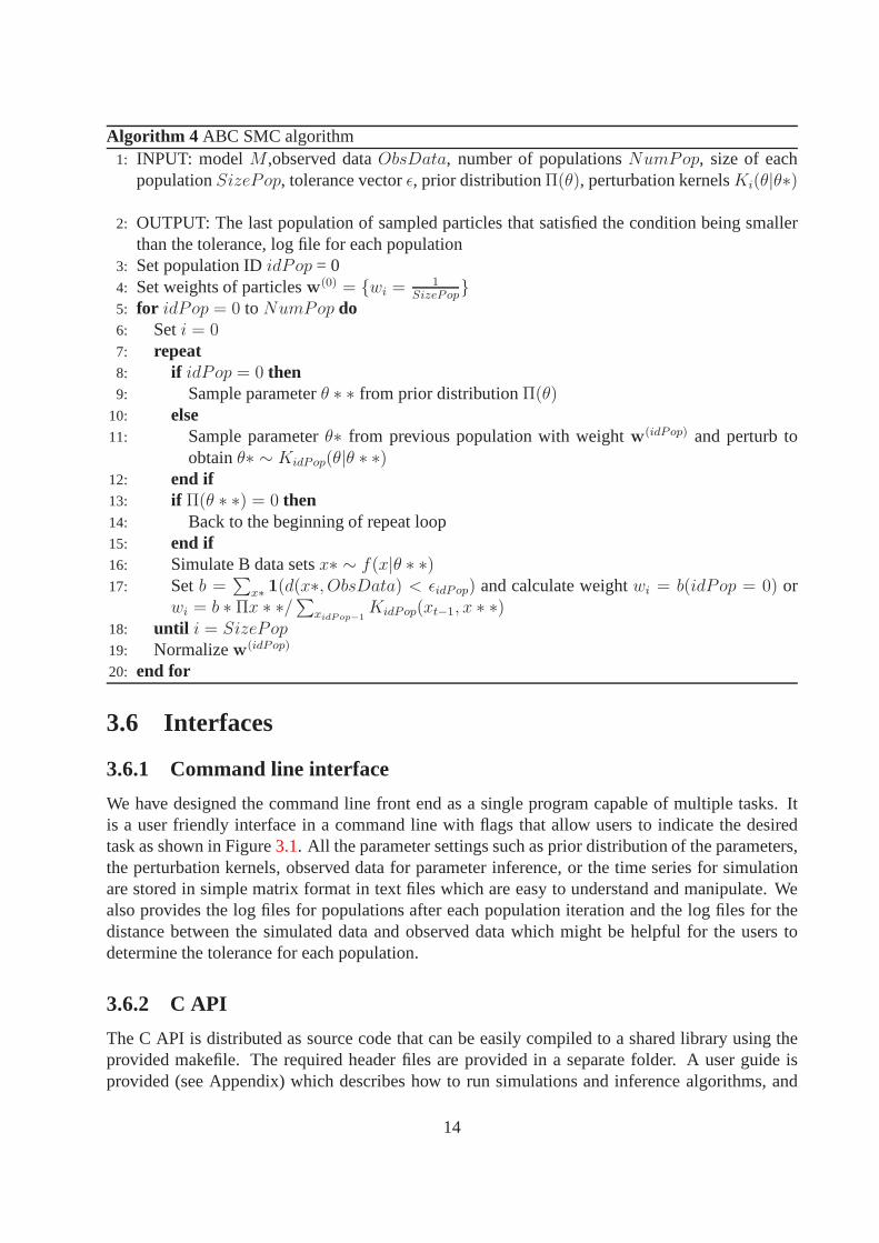
Algorithm 4 ABC SMC algorithm1: INPUT: modelM ,observed dataObsData, number of populationsNumPop, size of each

populationSizePop, tolerance vectorǫ, prior distributionΠ(θ), perturbation kernelsKi(θ|θ∗)

2: OUTPUT: The last population of sampled particles that satisfied the condition being smallerthan the tolerance, log file for each population

3: Set population IDidPop = 04: Set weights of particlesw(0) = {wi = 1

SizePop}

5: for idPop = 0 to NumPop do6: Seti = 07: repeat8: if idPop = 0 then9: Sample parameterθ ∗ ∗ from prior distributionΠ(θ)

10: else11: Sample parameterθ∗ from previous population with weightw(idPop) and perturb to

obtainθ∗ ∼ KidPop(θ|θ ∗ ∗)12: end if13: if Π(θ ∗ ∗) = 0 then14: Back to the beginning of repeat loop15: end if16: Simulate B data setsx∗ ∼ f(x|θ ∗ ∗)17: Setb =

∑

x∗ 1(d(x∗, ObsData) < ǫidPop) and calculate weightwi = b(idPop = 0) orwi = b ∗ Πx ∗ ∗/ ∑

xidPop−1KidPop(xt−1, x ∗ ∗)

18: until i = SizePop19: Normalizew(idPop)

20: end for

3.6 Interfaces

3.6.1 Command line interface

We have designed the command line front end as a single program capable of multiple tasks. Itis a user friendly interface in a command line with flags that allow users to indicate the desiredtask as shown in Figure3.1. All the parameter settings such as prior distribution of the parameters,the perturbation kernels, observed data for parameter inference, or the time series for simulationare stored in simple matrix format in text files which are easyto understand and manipulate. Wealso provides the log files for populations after each population iteration and the log files for thedistance between the simulated data and observed data whichmight be helpful for the users todetermine the tolerance for each population.

3.6.2 C API

The C API is distributed as source code that can be easily compiled to a shared library using theprovided makefile. The required header files are provided in aseparate folder. A user guide isprovided (see Appendix) which describes how to run simulations and inference algorithms, and

14

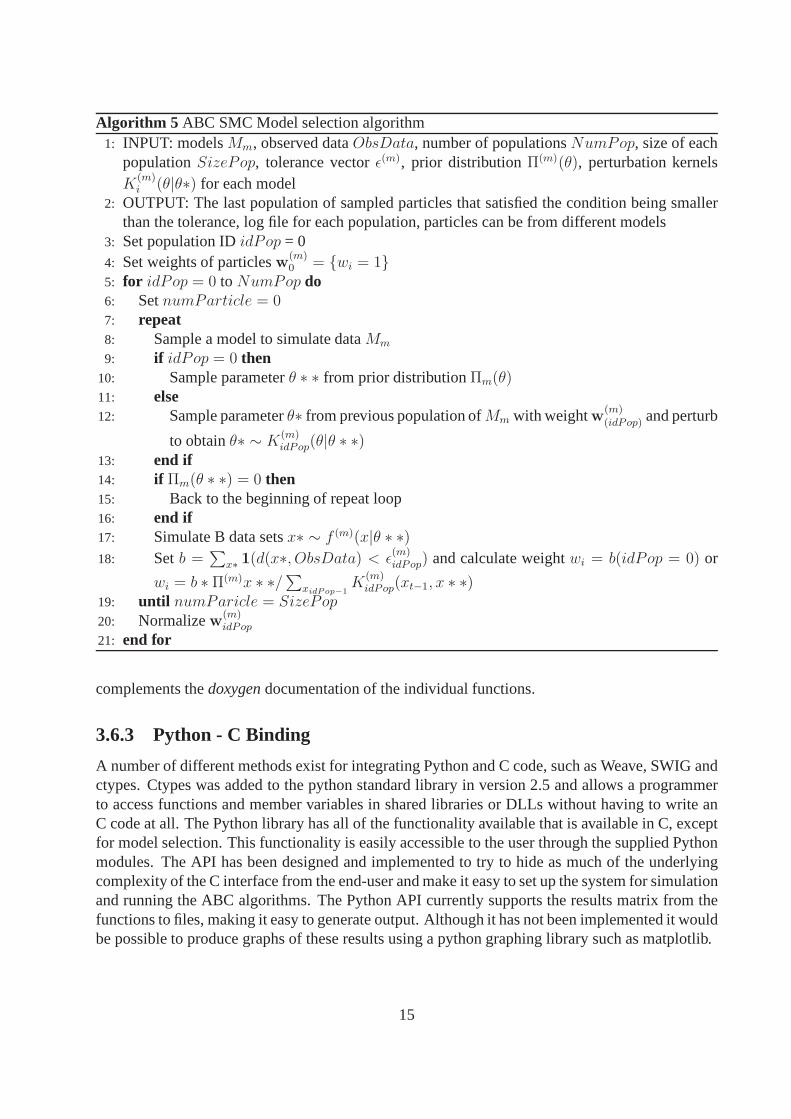
Algorithm 5 ABC SMC Model selection algorithm1: INPUT: modelsMm, observed dataObsData, number of populationsNumPop, size of each

populationSizePop, tolerance vectorǫ(m), prior distributionΠ(m)(θ), perturbation kernelsK

(m)i (θ|θ∗) for each model

2: OUTPUT: The last population of sampled particles that satisfied the condition being smallerthan the tolerance, log file for each population, particles can be from different models

3: Set population IDidPop = 04: Set weights of particlesw(m)

0 = {wi = 1}5: for idPop = 0 to NumPop do6: SetnumParticle = 07: repeat8: Sample a model to simulate dataMm

9: if idPop = 0 then10: Sample parameterθ ∗ ∗ from prior distributionΠm(θ)11: else12: Sample parameterθ∗ from previous population ofMm with weightw(m)

(idPop) and perturb

to obtainθ∗ ∼ K(m)idPop(θ|θ ∗ ∗)

13: end if14: if Πm(θ ∗ ∗) = 0 then15: Back to the beginning of repeat loop16: end if17: Simulate B data setsx∗ ∼ f (m)(x|θ ∗ ∗)18: Setb =

∑

x∗ 1(d(x∗, ObsData) < ǫ(m)idPop) and calculate weightwi = b(idPop = 0) or

wi = b ∗ Π(m)x ∗ ∗/∑

xidPop−1K

(m)idPop(xt−1, x ∗ ∗)

19: until numParicle = SizePop20: Normalizew(m)

idPop

21: end for

complements thedoxygendocumentation of the individual functions.

3.6.3 Python - C Binding

A number of different methods exist for integrating Python and C code, such as Weave, SWIG andctypes. Ctypes was added to the python standard library in version 2.5 and allows a programmerto access functions and member variables in shared libraries or DLLs without having to write anC code at all. The Python library has all of the functionalityavailable that is available in C, exceptfor model selection. This functionality is easily accessible to the user through the supplied Pythonmodules. The API has been designed and implemented to try to hide as much of the underlyingcomplexity of the C interface from the end-user and make it easy to set up the system for simulationand running the ABC algorithms. The Python API currently supports the results matrix from thefunctions to files, making it easy to generate output. Although it has not been implemented it wouldbe possible to produce graphs of these results using a pythongraphing library such as matplotlib.

15

3.6.4 R interface

The R interface includes seven R functions, each of which include the SBML parser. There arefour solvers (Ordinary Differential Equations, Delay-Differential Equations, Chemical LangevinEquations and Multi-Compartment Gillespie) and three ABC methods (Rejection, MCMC andSMC). Due to the nature of R’s internal structures and its C interfacing functions, the R version ofour package is simple to use but it does not have the same user manipulability as the C and Pythonversions. Brief descriptions of the functions and the differences between the versions are listedbelow.

The package consists of R wrapper functions which then call the appropriate C wrapper func-tions which then call the appropriate C functions. Because of the internal structures of R and thedesire to have our package also be a stand alone C package, we needed both R and C wrapperfunctions. Unfortunately for the users, this means the source code will not be as readily avaible tosearch through and modify.

The complex nature of our package required us to make use of the R function .Call, which isnewer and less documented than the standard .C function. Thepackage makes use of the R macrosfound in the R header files (R.h, Rinternals.h and Rdefines.h). The header files are included in thestandard installation of R.

The package is currently only suppored on UNIX type systems and MAC OS X; with thepackage submission to CRAN, it should be made available on Windows as well.

SBMLodeSolve()

SBMLodeSolve() takes an SBML file and a vector of times to sample; it returns a matrix consistingof the sample times and the populations for each of the species in the reactions. There is a choicebetween 10 differential equation solvers, two of which are stiff differenetial equation solvers. Inthe C version, the user can define their own gradiant functions;this feature is not available in the Rversion.

SBMLddeSolve

SBMLodeSolve() takes an SBML file and a vector of times to sample; it returns a matrix consistingof the sample times and the populations for each of the species in the reactions. It is a dely-differential equation solver. In the C version, the user candefine their own gradiant functions; thisfeature is not avalible in the R version.

SBMLcleSolve

SBMLcleSolve() takes an SBML file and a vector of times to sample; it returns a matrix consistingof the sample times and the populations for each of the species in the reactions. It is a stochasticsolver, with the option to run Tau Leaping or Chemical Langevin Equation. In the C version, theuser can define their own propensity functions; this featureis not avaiable is not availible in the Rversion.

16

SBMLgillSolve

SBMLgillSolve() takes an SBML file and a vector of times to sample; it returns a matrix consistingof the sample times and the populations for eacg of the species in the reactions. It is a stochasticsolver using a multi-compartment Gillespie algorithm and there is no loss of functionality betweenthe C and R versions.

SBMLabcRej

SBMLabcRej() takes an SBML file, an observed data file, a vector of prior distribution types,two vectors describing the prior disribution settings, thenumber of samples, the solver type, thethreshold on the distance measure, the maximum number of iterations and the output file name.It returns a matrix of the accepted values of the last population. In the C version, the user canpass their own function to set the parameters, they can choose their own distance metric and theycan choose whether or not missing data is included in the algorithm. In the R version, the setparameters function is default, the distance metric is sum of squares, and the algorithm does notinclude missing data.

SBMLabcMCMC

SBMLabcMCMC() takes an SBML file, an observed data file, a vector of prior distribution types, avector of kernel distribution types, two vectors describing the prior disribution settings, two vectorsdescribing the kernel distribution settings, the number ofsamples, the solver type,a vector of initalparameter settings, the threshold on the distance measure,and the output file name. It returns amatrix of the accepted values of the last population. In the Cversion, the user can specify whichdistance metric to use and how to deal with missing data. In the R version, the distance is set tosum of squares and the missing data is included.

SBMLabcSMC

SBMLabcSMC takes an SBML file, an observed data file, a vector of prior distribution types, twovectors of prior distribution settings, a vector of Gaussian standard deviation for the perterbationkernel, a vector of distance measure thresholds for each population, the number of populations,the size of inital population, the number of stochastic simulations for each parameter and a outputfile name. In the C version, the user can define the distance metric, the handling of missing data,set the perterbation kernel for each population and the ability to recover the previous population ofsamples particles if the simulation is halted. In the R version, the distance metric is sum of squares,missing data is included, the perterbation kernel is set forall populations and there is no recoverymechanism.

17

Figure 3.1: Screen shot of instruction on how to use the the programsbmlabc

18

Chapter 4

Examples and results

4.1 Data simulation

4.1.1 Lotka-Volterra model

The Lotka-Volterra (LV) model is a classic model describingthe relation between preys and preda-tors in an ecological system. The model is described by the reactions:

X → 2X with ratec1 (4.1)

X + Y → 2Y with ratec2 (4.2)

Y → Ø with ratec3 (4.3)

whereX denotes the prey andY denote the predator.The stochastic simulation of this model with Gillespie’s algorithm with initial condition(X, Y ) =

(1000, 1000) with the set of parameters(c1, c2, c3) = (10, 0.01, 10) is shown in Figure4.1, showingthe oscillatory characteristic of the model.

0 5 10 15 20

500

1000

1500

2000

time

Figure 4.1: Lotka-Volterra simulated using Gillespie’s algorithm.

19

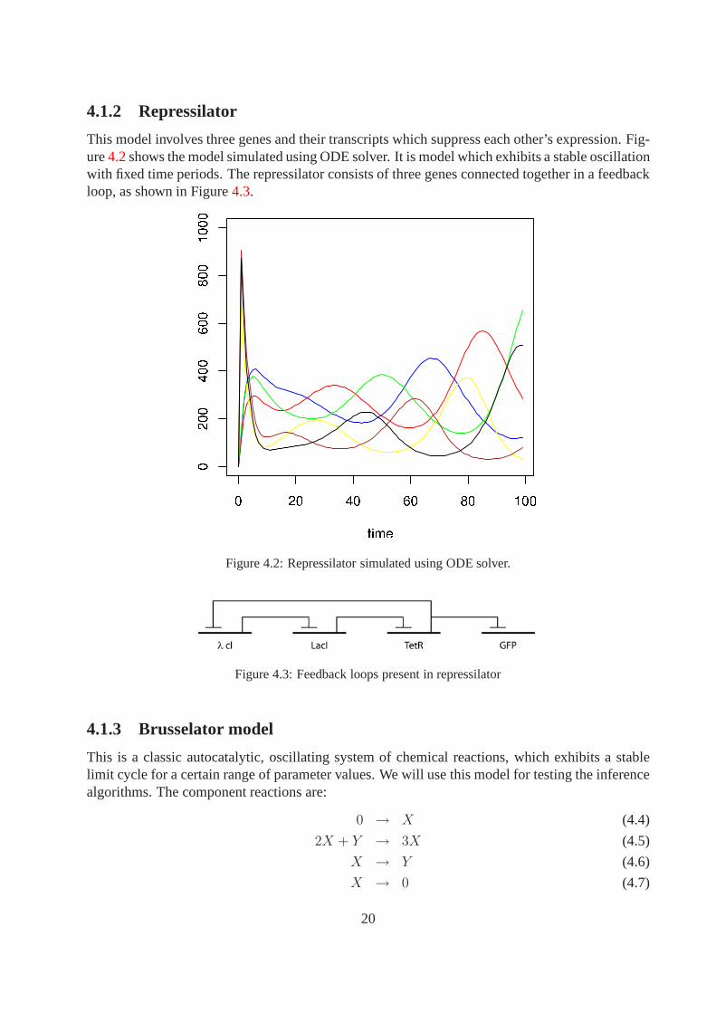
4.1.2 Repressilator

This model involves three genes and their transcripts whichsuppress each other’s expression. Fig-ure4.2shows the model simulated using ODE solver. It is model whichexhibits a stable oscillationwith fixed time periods. The repressilator consists of threegenes connected together in a feedbackloop, as shown in Figure4.3.

Figure 4.2: Repressilator simulated using ODE solver.

Figure 4.3: Feedback loops present in repressilator

4.1.3 Brusselator model

This is a classic autocatalytic, oscillating system of chemical reactions, which exhibits a stablelimit cycle for a certain range of parameter values. We will use this model for testing the inferencealgorithms. The component reactions are:

0 → X (4.4)

2X + Y → 3X (4.5)

X → Y (4.6)

X → 0 (4.7)

20

The ODEs are just in terms of the rate constants:

d[X]

dt= p1 + p2[X]2[Y ] − p3[X] − p4[X] (4.8)

d[Y ]

dt= −p2[X]2[Y ] + p3[X] (4.9)

The Jacobian of system of ODEs:

dxi

dt= Fi(x1, . . . , xn) (4.10)

is given by

Jij =∂Fi

∂xj

(4.11)

So for this model,

J =

[

2p2[X][Y ] − p3 − p4 p2[X]2

−2p2[X][Y ] + p3 −p2[X]2

]

(4.12)

Figure4.4shows simulations of this model using four different simulation algorithms.

4.2 Parameter inference

We initially tested the inference algorithms on the Brusselator model and artificial observed datawith 100 time points.

4.2.1 ABC rejection

ABC rejection was run requiring 1000 accepted samples, sum of squares distance function, and atolerance ofǫ = 5× 106. This level ofǫ across 100 time points and 2 species corresponds to a rootmean square error (RMSE) of 158, where the species concentration peaks are around 1000. Therun required a total of 319967 samples, giving an acceptanceratio of 0.31%. Figure4.5(a)showsa histogram for parameter 1 (the rate of reaction 1) over the 1000 samples. Figure4.5(b)showsthe accepted samples plotted as parameter 1 (the rate of reaction 1) against parameter 2 (the rate ofreaction 2). It is more informative to investigate plots of one parameter against another than simplehistograms of one parameter as this highlights correlations between parameters.

To put theǫ = 5 × 106 threshold into context it is interesting to compare simulated data thatwas accepted to the observed data, as shown in Figures4.6(a)and4.6(b).

4.2.2 ABC MCMC

ABC MCMC was run with the same epsilon threshold of5 × 106. For 1000 accepted samples90204 time courses were generated, giving an acceptance ratio of 1.1%. As expected this is slightlyhigher than for rejection, but it is at the cost of correlatedsamples. Figure4.7(b)shows parameter 1

21

0 20 40 60 80 100

0200

400

600

800

1000

time/s

(a) Ordinary Differential Equation solver (b) Tau leap

(c) Chemical Langevin Equation solver (d) Gillespie’s algorithm

Figure 4.4: Simulations of the Brusselator model using different algorithms.

22

(a) Histogram of parameter 1

0.3 0.4 0.5 0.6 0.7 0.8 0.9 1.0

0.5

1.0

1.5

2.0

p_1, true = .5p_4, true = 1

(b) Parameter 1 vs. 4 samples

Figure 4.5: Results of ABC rejection on Brusselator model using ODE solver.

(a) Species 1 (b) Species 2

Figure 4.6: Observed data (blue) and accepted simulated data (gray lines).

23

(a) Histogram of parameter 1

0.3 0.4 0.5 0.6 0.7 0.8 0.9 1.0

0.5

1.0

1.5

2.0

p_1, true = .5

p_4, true = 1

(b) Parameter 1 vs. 4 samples

Figure 4.7: Results of ABC MCMC on Brusselator model using ODE solver.

against 4 for accepted samples, and the agreement with the range of feasible values from rejectionis very good.

Figure4.8(a)shows a histogram of all the distances calculated during therun. The threshold weuse corresponds tolog10(5×106) = 6.7, so we see that just the tail is accepted. Figure4.8(b)showsthe distribution of the distances calculated. Significantly less very large distances are produced,which corresponds to the the fact that unlike rejection, MCMC does not waste many samples inregions of low probability.

(a) Rejection

log_10(distance)

5 6 7 8 9

05000

15000

25000

(b) MCMC

Figure 4.8: Histograms of log(distance) for all simulated datasets.

24

4.2.3 ABC SMC

ABC SMC was run for Brusselator using RKF45 ODE solver. 1000 particles were used with 8populations, withǫ decreasing linearly from107 to 3 × 106. The number of samples required foreach population, and the corresponding acceptance ratio are shown in Table4.1. The acceptanceratio decreases as the threshold decreases, as expected. This can be clearly seen in Figure4.10,which shows the roughly exponential relationship between the acceptance ratio andǫ. It wouldbe interesting to try reducing the width of the perturbationkernel through the populations, as thismight help the samples stay in regions of higher probability. It would also be interesting to seeif further reduction ofǫ was possible, as it appears that the reduction from5 × 106 to 3 × 106

actually has little effect on the acceptance ratio. Figure4.9 shows plots of parameter 1 vs. 4 forthe successive populations. The samples start out relatively diffuse, and concentrate on regions ofhigher posterior probability as the threshold is decreased. It is interesting that for large values ofǫa second mode with parameter 1 close to zero is possible, but which is eliminated asǫ is reduced.

Population ǫ/106 # simulations Acceptance ratio1 10 6772 0.1476672 9 17977 0.0556273 8 23389 0.0427554 7 34253 0.0291955 6 59936 0.0166846 5 290406 0.0034437 4 224550 0.0044538 3 299915 0.003334

Table 4.1: Statistics for each population of ABC SMC.

4.3 Model selection

We did an experiment with observed data generated from the Brusselator model with ODE solverto observe the performance of the model selection algorithm. We assumed that the data is froman unknown source and the objective is to try different models to see which one best describes thebehaviour of the model.

We did model selection with two models: the Brusselator model itself and the Lotka-Volterramodel, both simulated using Gillespie’s algorithm. The settings for parameters for each model(perturbation kernel and prior distributions) are set separately, however the tolerances, the markvector and so on are shared between the two. The algorithm wasrun for 5 populations to generate100 parameter vectors. The results show that from the first population of parameters, only Brus-selator model is present. Consequently, in the following populations, only the Brusselator modelremains.

This result shows that the model selection was able to correctly choose the model which bestpredicts the unknown observed data.

25

(a) Populations 1 (red) and 2 (orange) (b) ...plus populations 3 (light green) and 4 (green)

(c) ...plus populations 5 (light blue) and 6 (blue) (d) ...plus populations 7 (purple) and 8 (magenta)

Figure 4.9: Parameter 1 vs. 4 from ABC SMC with 8 populations,1000 particles on Brusselator using ODEsolver. Populations are shown added two per plot.

26

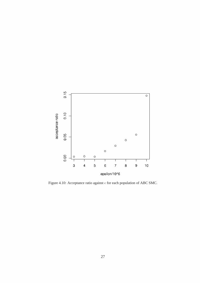
Figure 4.10: Acceptance ratio againstǫ for each population of ABC SMC.

27

Chapter 5

Future work

Additional simulation algorithms. Various other simulation algorithms could be valuable ad-ditions to the package. Additional stochastic algorithms include the Next Reaction method (Gib-son & Bruck), more advanced tau leaping algorithms (e.g. implicit tau leap), and higher orderStochastic Differential Equations than the CLE. Hybrid algorithms involving both stochastic anddeterministic components are available which choose the most appropriate for each reaction andspecies.

Advanced implementations. Monte Carlo algorithms are good candidates for parallelisation.Technologies such as CUDA might offer a good way of improvingsimulation throughput, althoughthis would mean that the package would be tied to a specific vendor, which may not be ideal. Itmay be possible to create an MPI or OpenMP enabled version of the package which could meanthat the algorithms could be run on high performance computing resources. Difficulties do existhowever with implementing efficient and robust random number generation across a distributedenvironment.

Random number generator. It could be valuable to investigate the use of a different randomnumber generator. Other random number generators are available that have longer periods, are justas random and are less computationally intensive to compute[26]. Since a lot of random numbersare generated by our system this could lead to a reduction in compute time whilst not impactingon the soundness of the algorithm.

Distance measures. The existing distance measures calculate only the error in the dependentvariable, i.e. the species. This means that very similar observed and simulated data which isslightly misaligned in time will have an undesirably large distance. As a result samples may berejected which actually represent quite good parameters. Some kind of time shift invariant distancefunction, or inference of an initial lag in the model, could be ways of addressing this problem.

Automatic conversion between stochastic and deterministic models Currently it is not possi-ble to take a model encoded with stochastic parameters and simulate this deterministically and getresults which make sense.

28

Lyapunov exponents. How close the samples ABC produced are to being samples from the trueposterior will clearly depend on to what extent similar datacorresponds to similar parameters. Forinferring initial conditions especially, this is closely related to Lyapunov exponents as they con-trol the rate of divergence from different starting conditions. Functionality to estimate Lyapunovexponents could therefore be a useful addition.

Improved data structure for MCMC. The MCMC algorithm stores duplicates of the currentvector of parameters every time a sample is rejected. As a result a single vector is stored manytimes in the output matrix. A more efficient structure would simply store unique vectors and thenumber of repeats of each.

Autocorrelation times for MCMC. For evaluating how long the burn in period of an MCMCalgorithm is it is useful to be able to estimate the integrated autocorrelation time of the samples:the burn in period should be at least this long. Built in functionality to achieve this would be veryuseful.

29

Acknowledgements

We would like to thank Tina, Kamil, Paul and Michael for theirsupport and advice.Nathan would like to thank nature for evolvingCamellia Sinensis.

30

Bibliography

[1] M. Hucka, A. Finney, H. M. Sauro, H. Bolouri, J. C. Doyle, and H. Kitano. The systemsbiology markup language (sbml): a medium for representation and exchange of biochemicalnetwork models.Bioinformatics, 19(4):524–531, 2003.

[2] P. Marjoram, J. Molitor, V. Plagnol, and S. Tavare. Markov chain Monte Carlo withoutlikelihoods.Proc Natl Acad Sci U S A, 100(26):15324–15328, 2003.

[3] Stefan Hoops, Sven Sahle, Ralph Gauges, Christine Lee, Jrgen Pahle, Natalia Simus, Mu-dita Singhal, Liang Xu, Pedro Mendes, and Ursula Kummer. Copasi–a complex pathwaysimulator.Bioinformatics, 22(24):3067–3074, Dec 2006.

[4] Zhike Zi and Edda Klipp. Sbml-pet: a systems biology markup language-based parameterestimation tool.Bioinformatics, 22(21):2704–2705, Nov 2006.

[5] Xinglai Ji and Ying Xu. libsres: a c library for stochastic ranking evolution strategy forparameter estimation.Bioinformatics, 22(1):124–126, Jan 2006.

[6] A.C. Hindmarsh. Odepack, a systematized collection of ode solvers. In R.S. et al. Stepleman,editor, Scientific Computing: Applications of Mathematics and Computing to the PhysicalSciences, volume 1 ofIMACS Transactions on Scientific Computing, pages 55–64, Amster-dam, Netherlands; New York, U.S.A., 1983. North-Holland.

[7] Benjamin J Bornstein, Sarah M Keating, Akiya Jouraku, and Michael Hucka. Libsbml: anapi library for sbml.Bioinformatics, 24(6):880–881, Mar 2008.

[8] Gillespie D.T. A general method for numerically simulating the stochastic time evolution ofcoupled chemical reactions.Journal of Computational Physics, 22:403–34, 1976.

[9] Gillespie D.T. Exact stochastic simulation of coupled chemical reactions.Journal of Com-putational Physics, 81:2340–61, 1977.

[10] Gibson M.A. and Bruck J. Exact stochastic simulation ofchemical system with many speciesand many channels.Journal of Physical Chemistry, 105:1876–89, 2000.

[11] Gillespie D.T. The chemical langevin equation.Journal of Chemical Physics, 113:297306,2000.

[12] Gillespie D.T. Approximate accelerated stochastic simulation of chemically reacting systems.Journal of Chemical Physics, 115:171633, 2001.

31

[13] Gillespie D.T. and Petzold L.R. Improved leap-size selection for accelerated stochastic sim-ulation. Journal of Chemical Physics, 119:822934, 2003.

[14] Cao Y.and Petzold L.R. Improved leap-size selection for accelerated stochastic simulation.Journal of Chemical Physics, 124:044109, 2006.

[15] Paun Gh. Computing with membranes.Journal of Computer and System Sciences,61(1):108–143, 2000.

[16] Priami C. and Plotkin G.(Eds.). P systems, a new computational modelling tool for systemsbiology. Transaction on computational Systems Biology VI, LNBI 4220:176–197, 2006.

[17] Toni T., Welch D., Stumpf M.P.H., and et al. Approximatebayesian computation scheme forparameter inference and model selection in dynamical systems. in press, 2008.

[18] Brad Chapman and Jeffrey Chang. Biopython: Python tools for computational biology.SIG-BIO Newsl., 20(2):15–19, 2000.

[19] R Development Core Team.R: A Language and Environment for Statistical Computing. RFoundation for Statistical Computing, Vienna, Austria, 2007. ISBN 3-900051-07-0.

[20] Tomas Radivoyevitch. A two-way interface between limited systems biology markup lan-guage and r.BMC Bioinformatics, 5:190, Dec 2004.

[21] Pritchard J.K., Seielstad M.T., Perez-Lezaun A., and Feldman M.W. Population growth ofhuman Y chromosomes: a study of Y chromosome microsatellites. Molecular BiologicalEvolution, 16(12):1791–1798, 1999.

[22] S. A. Sisson, Y. Fan, and Mark M. Tanaka. Sequential monte carlo without likelihoods.PNAS, 104(6):1760–1765, 2007.

[23] Del Moral P. and Jasra A. Sequential monte carlo samplers. Journal of Royal StatisticsSociety B, 68(3):411–436, 2006.

[24] Del Moral P. and Jasra A. Sequential monte carlo for bayesian computation.in press, 2008.

[25] Robert E. Kass and Adrian E. Raftery. Bayes factors.Journal of the American StatisticalAssociation, 90(430):773–795, 1995.

[26] George Marsaglia and Arif Zaman. A new class of random number generators.The Annalsof Applied Probability, 1(3):462–480, 1991.

32