Accelerating Monte Carlo Analysis at Advanced Nodes · PDF fileworst-case circuit ... Initial Monte Carlo simulation automatically stops when a response surface model can be ... Accelerating

Introduction

Remember when all you had to worry about were process, voltage, and temperature (PVT) corners? This was a fairly complicated task in and of itself, involving up to double-digit process corners as well as the temperature and voltage sweeps. You might have run Monte Carlo analysis, but it took such a long time, and what you had to do to resolve problems was not always clear.

Now, every time you scale down a design, the relative variation gets bigger. As the design shrinks, it simply becomes harder to control the precision of every step in the manufacturing process. That’s why the importance of statistical variation (and its impact) increases for every node, and accurately and efficiently dealing with variation has become more important than ever in advanced nodes.

How do you avoid overdesigning to accommodate PVT effects? Or missing your deadlines? New fast Monte Carlo analysis technology helps you efficiently prevent loss of yield and performance, identifying problems prior to layout so you can resolve them early on and stay on schedule. Let’s first outline why traditional corner-based methods are inaccurate and traditional Monte Carlo analysis is inefficient at advanced nodes to show how the new technology overcomes these issues.

Accelerating Monte Carlo Analysis at Advanced Nodes By Lucas Zhang, Sr Principal Software Engineer; Hongzhou Liu, Software Engineering Director; and Steve Lewis, Product Management Director, Cadence

Advanced-node designs have much larger variation, making it much more difficult to achieve high yields at these processes. But can you really afford to run thousands or even millions of statistical simulations to predict how well your design will meet its specs? Or overdesign to accommodate manufacturing variations? In this paper, we will introduce a fast Monte Carlo analysis technique that delivers foundry-certified metrics you can rely on to produce high-quality advanced-node designs and meet aggressive project schedules.

ContentsIntroduction ......................................1

Why Traditional Methods Face Difficulties at Advanced Nodes ..........2

Advantages of a Variation-Aware Design Methodology ........................2

Two Algorithms for Fast, Accurate 3-Sigma Corner Creation ...................3

Mismatch Contribution ......................5

Efficient Yield Verification Via Sample Reordering ............................6

Fast Monte Carlo Analysis for High-Yield Designs .......................8

Summary ...........................................9

For Further Information .....................9

Why Traditional Methods Face Difficulties at Advanced Nodes

At 16nm and below, variation has become so significant that traditional approaches to control it, like using foundry-provided corners characterized for digital circuits, are breaking down, resulting in much less accuracy. Monte Carlo analysis provides an option for accurately capturing statistics on circuit behavior to help you evaluate performance.

However, a big drawback of the traditional Monte Carlo approach is that it typically requires a large volume of samples to provide a more accurate picture of design yield. That’s a time-consuming proposition. What if you had a technique that yielded the same accuracy as 100,000 simulation runs in only a few hundred runs? What if you were clear on exactly which design parameters you need to tune? What if you had a way to be confident that your yield will be good—without spending a few weeks doing simulation?

Advantages of a Variation-Aware Design Methodology

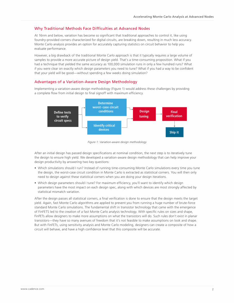
Implementing a variation-aware design methodology (Figure 1) would address these challenges by providing a complete flow from initial design to final signoff with maximum efficiency.

Identify criticaldevices

Design

tuning Final

verification

Ship it

Define tests to verify

circuit specs

Determine worst - case circuit

conditions

Figure 1: Variation-aware design methodology

After an initial design has passed design specifications at nominal condition, the next step is to iteratively tune the design to ensure high yield. We developed a variation-aware design methodology that can help improve your design productivity by answering two key questions:

• Which simulations should I run? Instead of running time-consuming Monte Carlo simulations every time you tune the design, the worst-case circuit condition in Monte Carlo is extracted as statistical corners. You will then only need to design against these statistical corners when you are doing your design iterations.

• Which design parameters should I tune? For maximum efficiency, you’ll want to identify which design parameters have the most impact on each design spec, along with which devices are most strongly affected by statistical mismatch variation.

After the design passes all statistical corners, a final verification is done to ensure that the design meets the target yield. Again, fast Monte Carlo algorithms are applied to prevent you from running a huge number of brute-force standard Monte Carlo simulations. The fundamental shift in transistor technology that came with the emergence of FinFETS led to the creation of a fast Monte Carlo analysis technology. With specific rules on sizes and shape, FinFETs allow designers to make more assumptions on what the transistors will do. Such rules don’t exist in planar transistors—they have so many avenues of freedom that it’s not feasible to make assumptions on look and shape. But with FinFETs, using sensitivity analysis and Monte Carlo modeling, designers can create a composite of how a circuit will behave, and have a high confidence level that this composite will be accurate.

www.cadence.com 2

Accelerating Monte Carlo Analysis at Advanced Nodes

Two Algorithms for Fast, Accurate 3-Sigma Corner Creation

Traditional Monte Carlo Analysis typically verifies a 3-sigma yield. Since 3-sigma corresponds to only a 0.13% probability, verification requires a large sample size, as noted in Table 1.

Confidence Number of Samples

80% 1200

90% 1700

95% 2200

Table 1. Samples required to verify 3-sigma yield at varying levels of confidence

Given the size of this verification effort, it’s useful to extract and design against 3-sigma corners from a small number of ordinary Monte Carlo samples. In order to speed up the overall circuit analysis while delivering the desired accuracy, we developed two algorithms for faster corner creation.

K-Sigma Corners Algorithm

The first algorithm, called K-Sigma Corners, creates 3-sigma corners with only up to 200 Monte Carlo samples (by comparison, brute-force Monte Carlo analysis generally requires 2,000 samples). Each 3-sigma corner is circuit- and performance-dependent. The first step is to extract the 3-sigma target value. In a normal distribution, the 3-sigma target can be estimated by mean + 3*std. If the distribution isn’t normal, we can fit the distribution from a distribution family extended from normal. Which distribution to use can automatically be determined by a normality test to achieve the optimal tradeoff between speed and accuracy.

Next, we need to extract the corner that matches the target via a smart fitting algorithm that models the performance as a function of process parameters. If the extracted corner doesn’t match the target well, such as in some highly nonlinear outputs, then we can adjust the corner by searching on the line connecting the nominal point and the corner from the model (this search can take up to 11 additional simulations, but most of the time, the corner is already accurate and only one additional simulation is needed).

The Monte Carlo run automatically stops when an accurate distribution model can be fit to extract the 3-sigma corners. As noted, it takes up to 200 samples to fit a model for 3-sigma corners, but for strongly linear outputs, only 50 points may be needed to fit the model. The design in question might already meet the target sigma; in this case, it’s not necessary to further improve the design against statistical corners. The probability that each spec already meets target is provided at the end of the K-Sigma Corners algorithm.

Worst Samples Algorithm

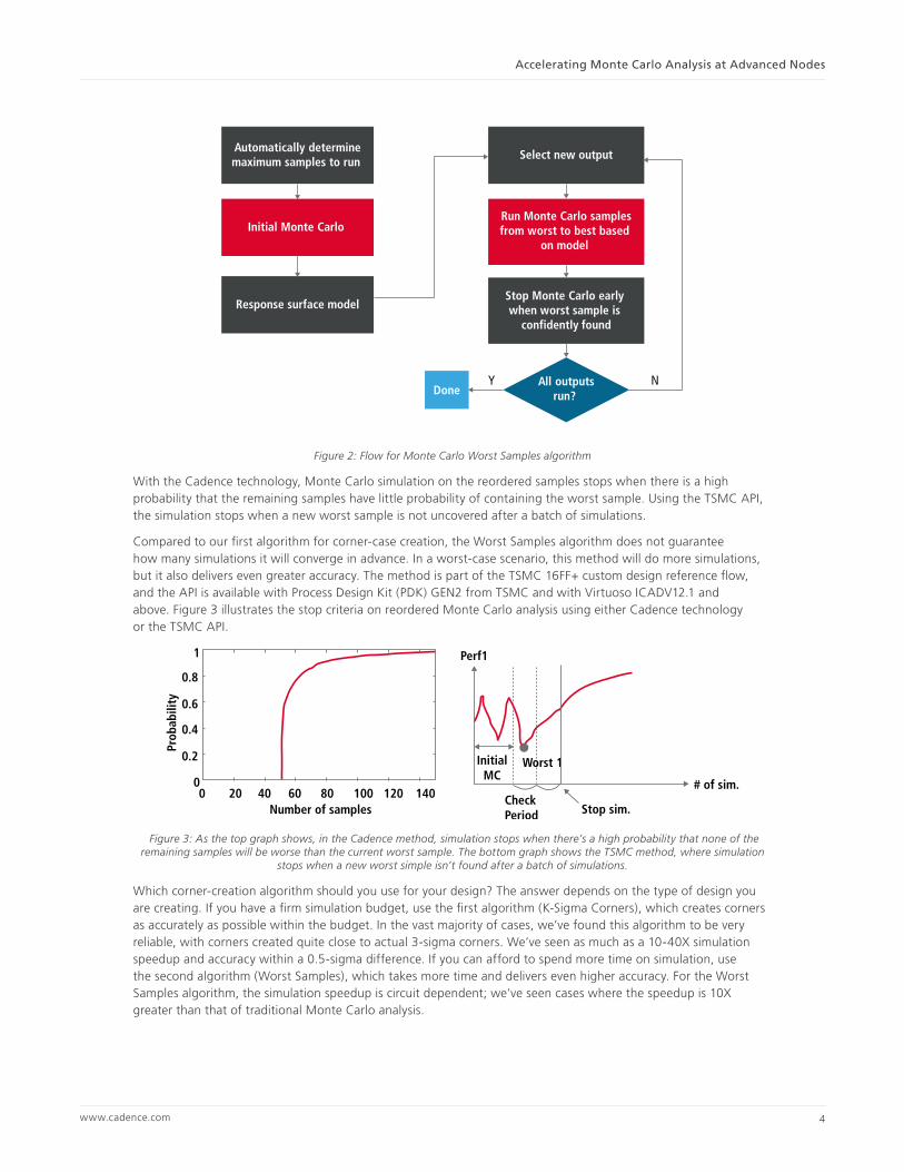
The second algorithm, the Worst Samples algorithm, applies Monte Carlo reordering to speed the analysis process without accuracy loss. In this algorithm, you’d need to do an initial sampling to build a response surface model and then model each output as a function of underlying statistical parameters. Our Worst Samples algorithm then runs Monte Carlo samples from worst to best based on the model; in other words, those most likely to fail are sampled first. The worst sample from each output is saved as a corner to replace Monte Carlo samples in future design iterations. Figure 2 illustrates the flow for this algorithm.

Initial Monte Carlo simulation automatically stops when a response surface model can be built for each spec.The model building process uses patented technology from Cadence (available in the Virtuoso® Variation Option and in the Virtuoso Analog Design Environment GXL (ADE GXL)) to significantly reduce the number of samples needed. Alternatively, you can also tap into critical device information from TSMC’s variation-aware API to further reduce the number of simulations needed. The API, which is tightly integrated with the Virtuoso ADE environment, essentially allows the Virtuoso ADE GXL and Virtuoso Variation Option to run sensitivity analysis to identify critical devices using a single variable per device. After an initial Monte Carlo run, each spec can be approximated by a model. Using the Cadence® technology, the model includes all statistical parameters. Using the TSMC method for each device, the six to seven mismatch parameters are reduced to one parameter representing Vth, which significantly reduces dimensionality.

www.cadence.com 3


Automatically determinemaximum samples to run

Stop Monte Carlo early when worst sample is

confidently found

Y N

Select new output

Run Monte Carlo samplesfrom worst to best based

on model Initial Monte Carlo

Response surface model

All outputsrun? Done

Figure 2: Flow for Monte Carlo Worst Samples algorithm

With the Cadence technology, Monte Carlo simulation on the reordered samples stops when there is a high probability that the remaining samples have little probability of containing the worst sample. Using the TSMC API, the simulation stops when a new worst sample is not uncovered after a batch of simulations.

Compared to our first algorithm for corner-case creation, the Worst Samples algorithm does not guarantee how many simulations it will converge in advance. In a worst-case scenario, this method will do more simulations, but it also delivers even greater accuracy. The method is part of the TSMC 16FF+ custom design reference flow, and the API is available with Process Design Kit (PDK) GEN2 from TSMC and with Virtuoso ICADV12.1 and above. Figure 3 illustrates the stop criteria on reordered Monte Carlo analysis using either Cadence technology or the TSMC API.

Perf1

Stop sim.

Worst 1

Check Period

InitialMC

# of sim.

Number of samples

Prob

abili

ty

0

1

0

0.4

0.2

0.6

0.8

20 40 60 80 100 120 140

Figure 3: As the top graph shows, in the Cadence method, simulation stops when there’s a high probability that none of the remaining samples will be worse than the current worst sample. The bottom graph shows the TSMC method, where simulation

stops when a new worst simple isn’t found after a batch of simulations.

Which corner-creation algorithm should you use for your design? The answer depends on the type of design you are creating. If you have a firm simulation budget, use the first algorithm (K-Sigma Corners), which creates corners as accurately as possible within the budget. In the vast majority of cases, we’ve found this algorithm to be very reliable, with corners created quite close to actual 3-sigma corners. We’ve seen as much as a 10-40X simulation speedup and accuracy within a 0.5-sigma difference. If you can afford to spend more time on simulation, use the second algorithm (Worst Samples), which takes more time and delivers even higher accuracy. For the Worst Samples algorithm, the simulation speedup is circuit dependent; we’ve seen cases where the speedup is 10X greater than that of traditional Monte Carlo analysis.

www.cadence.com 4


In experimental cases with our corner-creation algorithms, we experienced substantial simulation speedups. In a two-stage OpAmp example on the TSMC 16nm process, we measured gain, bandwidth, and phase margin (see Figure 4). We generated the worst samples for 1,832 Monte Carlo simulations (this figure is a conservative number for verifying 99.865% yield with 90% confidence).

Figure 4: Two-stage OpAmp example on TSMC 16nm process

In one Monte Carlo worst samples flow, we used Virtuoso ADE GXL, which automatically stopped its run at 201 points. The worst sample for every output matched full Monte Carlo simulation. We achieved a 9X simulation speedup in this experimental case. Next, we ran the flow with the TSMC variation-aware API. Here, Virtuoso ADE GXL automatically stopped the run at 110 points. The worst sample for gain and phase margin matched full Monte Carlo analysis, while the bandwidth output had a 1% error compared to the actual worst sample. In this second experimental case, we achieved a 17X simulation speedup.

Mismatch Contribution

Now, say you’ve found that your circuit still isn’t performing well on some corners. What else can you do to improve your design? There’s always designer intuition, but now you can also tap into technology that provides guidance on how you can optimize your design.

Mismatch contribution is one such technology, providing guidance on which devices are more important when it comes to variation. At advanced nodes, mismatch analysis is no longer optional, since variation can significantly impact circuit performance. After any Monte Carlo run, the mismatch contribution algorithm is available to identify important contributors to variance of circuit specifications due to device mismatch. The algorithm:

• Applies variance-based global sensitivity analysis

• Applies quadratic or linear models as needed

• Uses sparse regression techniques when there’s a large number of mismatch parameters

• Represents the model goodness of a fit by R^ 2

www.cadence.com 5


The mismatch contribution table in Figure 5 shows the percentage contribution of each device to the total variance of each specification. Each column can be sorted to easily view the largest contributors.

Select Test

SortableColumn forEach Spec

Hierarchialor Flat View

R^ 2 ModelAccuracy Metric

% Contributionto Total Variance

Figure 5: An example mismatch contribution table

Furthermore, the hierarchical view of mismatch contribution can be used to explore the mismatch contribution at each level of hierarchy. For example, Figure 6 shows a case where at the top level, the sub-circuit AmpOut contributes to 97% of the current variation, while AmpIn only contributes to 3%. By double-clicking the variance of Ampout, it is further revealed that most of the Ampout variation comes from the device M6. You can also interactively highlight device location in the schematic from the mismatch contribution table. This algorithm is available in the Virtuoso Variation Option and Virtuoso ADE GXL.

Figure 6: A hierarchical view of a mismatch contribution table

Efficient Yield Verification Via Sample Reordering

With the help of critical devices information from mismatch contribution, you are able to tune your design to pass all corners after several rounds of iterations. Now you just need to run a final Monte Carlo to signoff your circuit. Again, running a full Monte Carlo sampling requires around 2000 samples. Utilizing a yield verification algorithm that we created to provide sample reordering (Figure 7), you can sign off your circuit with the same confidence using much fewer samples.

www.cadence.com 6


Automatically determinemaximum samples to run

Stop Monte Carlo early with confidence• Yield target not met• Yield target met

Estimate the failure probability of each remaining sample

Run remaining Monte Carlosamples in new order of probability to fail

Perform initial Monte Carlo

Generate remaining MonteCarlo samples

Figure 7: Flow for Monte Carlo yield verification algorithm

Similar to the worst samples algorithm, an initial sampling is first performed to build a response surface model and then model each output as a function of underlying statistical parameters. The remaining samples are ordered based on their probability to fail any spec. Since the reordering does not need to be done on a per-specification basis, the yield verification algorithm typically runs faster than the worst samples algorithm.

MC Sample Number MC Sample Number

Spec Target

Stop

Yield Target

Initial MC Recorded MC

Figure 8: Stop criteria example for yield lower than target

The Monte Carlo sampling stops when either of the two conclusions can be confidently drawn: (1) yield is lower than target (Figure 8) or (2) yield is higher than target (Figure 9). To conclude that yield is lower than target, an upper bound in yield is generated from the Clopper-Pearson confidence interval by assuming all unsimulated samples will pass. When more failed samples are observed, the upper bound will decrease and the Monte Carlo run will stop when the upper bound is lower than the yield target. This method is much faster than standard Monte Carlo sampling because the failed samples will be simulated first, so that the conclusion is reached sooner.

www.cadence.com 7


MC Sample Number MC Sample Number

Stop

Yield Target

Spec Target

Initial MC Recorded MC

Figure 9: Stop criteria example for yield higher than target

To conclude that yield is higher than target, a lower bound in yield is generated from the Clopper-Pearson confidence interval. The number of failed samples used in lower bound estimation consists of two parts: the number of failed samples observed and the estimated number of failures in the future based on a conservative estimate of model accuracy. As more passed samples are observed, the lower bound will increase and the Monte Carlo run will stop when the lower bound is higher than the yield target. It will converge faster than standard Monte Carlo because the samples that are more likely to fail are simulated first, and we can stop when the probability of having any failures in the remaining samples is very low.

Using the same OpAmp example in the worst samples experiment, we first set the OpAmp to a high yield but less than 99.865%. It typically takes around 500 samples to gather a sufficient number of failed samples to conclude that yield is lower than the target. Our reordered yield verification algorithm found enough failed samples to stop the run at 58 points, a 9X speedup. We then configured the OpAmp to a very high yield, which would normally take 1700 samples to confirm that yield is greater than the target. Our algorithm made the same conclusion with 60 samples, a 28X speedup.

Fast Monte Carlo Analysis for High-Yield Designs

Many designs requiring high reliability—such as automotive systems—can no longer rely only on traditional Monte Carlo analysis because it is too time-consuming; they often require 4-6 sigma yield estimation. Our algorithm can predict circuit yield to 4-6 sigma without requiring the millions or billions of simulations that traditional Monte Carlo analysis would need. Scaled-Sigma Sampling gradually scales up the variation so that yield can be estimated using larger scaling factors (Figure 10). It has demonstrated accuracy for nonlinear behavior and efficiency for a large number of statistical parameters and specifications. (Our Scaled-Sigma Sampling paper recently received the 2016 IEEE Donald O. Pederson Best Paper Award, which recognizes the best paper published in the Transactions on Computer-Aided Design of Integrated Circuits and Systems over the past two years*.)

x(0, 0)

( )xfs 1=

( )xfs 2=

Ωx: process parameterΩ: failure region

Figure 10: The idea behind Scaled-Sigma Sampling is that, if we scale up the variation of all parameters by a factor of s, the failure rate P will typically increase.

With very general assumptions on the failure region, the failure rate can be modeled by

log (P) α+βlog(s)+γ⁄s2

www.cadence.com 8


The model coefficients (α, β, γ) can be estimated from Monte Carlo simulations at higher s. After fitting the model, the actual failure rate is

P(s=1)=exp(α+γ)

This method has proven accurate for high-yield designs and, since dimension information is encoded into the model coefficients, also for circuits with high-dimensionality. Scaled-Sigma Sampling has been tested on a large number of synthetic and real circuits (see Tables 2 and 3 for results). The Scaled-Sigma Sampling method can be used for both statistical corner creation and yield verification.

Test Case True Yield Estimated Yield 90% Conf Interval

Linear 6.0 5.89 5.27 6.63

Spherical 6.0 5.88 5.46 6.40

Parabolic 6.0 6.23 5.47 7.21

Table 2: Synthetic data results with 7000 samples

Test Case True Yield Estimated Yield 90% Conf Interval

SenseAmp Delay 5.0 4.83 4.29 5.78

SRAM Column Delay 4.5 4.66 4.27 5.05

OpAmp PSRR 4.5 4.63 4.20 5.12

OpAmp Random Offset 4.5 4.44 4.06 4.99

Table 3: Real circuit results with 7000 samples

Summary

When you need to ensure that the advanced-node design you’re sending to layout is the best that it can be—and you have a tight schedule to meet—you can’t afford to wait for millions of statistical simulations to run. Plus, at advanced nodes, the foundry-provided process corners characterized for digital circuits are no longer accurate. In this paper, we introduced a new flow that improves the productivity of advanced-node design through fast corner creation, fast signoff, and critical device detection. This flow delivers foundry-certified metrics that provide the circuit confidence you need to meet your yield targets.

For Further Information

Learn more about the Virtuoso Variation Option: http://www.cadence.com/products/cic/virtuoso_ade_product_suite/pages/default.aspx

Watch the Speed Up Monte Carlo Analysis for TSMC 16FF+ Design with the Virtuoso Analog Design Environment webinar: http://www.cadence.com/cadence/events/Pages/event.aspx?eventid=967

*Read the Scaled-Sigma Sampling paper: S. Sun, X. Li, H. Liu, K. Luo and B. Gu, “Fast statistical analysis of rare circuit failure events via Scaled-Sigma Sampling for high-dimensional variation space,” IEEE Trans. on Computer-Aided Design of Integrated Circuits and Systems, vol. 34, no. 7, pp. 1096-1109, Jul. 2015.

Cadence Design Systems enables global electronic design innovation and plays an essential role in the creation of today’s electronics. Customers use Cadence software, hardware, IP, and expertise to design and verify today’s mobile, cloud and connectivity applications. www.cadence.com

© 2016 Cadence Design Systems, Inc. All rights reserved. Cadence, the Cadence logo, and Virtuoso are registered trademarks of Cadence Design Systems, Inc. in the United States and other countries. All others are properties of their respective holders. 6486 06/16 CY/LA/PDF


9

Documents

Accelerating Monte Carlo Analysis at Advanced Nodes · PDF fileworst-case circuit ... Initial Monte Carlo simulation automatically stops when a response surface model can be ... Accelerating