Embed Size (px)
Citation preview
1
Access Methods for Markovian StreamsJulie Letchner #1, Christopher Re #2, Magdalena Balazinska #3, Matthai Philipose ∗4
#Computer Science & Engineering Department, University of WashingtonSeattle, Washington, USA
{1letchner, 2chrisre, 3magda}@cs.washington.edu∗Intel Research Seattle
Seattle, Washington, [email protected]
Abstract— Model-based views have recently been proposed asan effective method for querying noisy sensor data. Commonlyused models from the AI literature (e.g., the hidden Markovmodel) expose to applications a stream of probabilistic andcorrelated state estimates computed from the sensor data. Manyapplications want to detect sophisticated patterns of states fromthese Markovian streams. Such queries are called event queries.
In this paper, we present a new storage manager, Caldera,for processing event queries over stored Markovian streamsin the Lahar system. At the heart of Caldera is a set ofaccess methods for Markovian streams that can improve eventquery performance by orders of magnitude compared to existingtechniques, which must scan the entire stream. Our accessmethods use new adaptations of traditional B+ tree indexes,and a new index, called the Markov-chain index. They efficientlyextract only the relevant timesteps from a stream, while retainingthe stream’s Markovian properties. We have implemented ourprototype system on BDB and demonstrate its effectiveness onboth synthetic data and real data from a building-wide RFIDdeployment.
I. I
Applications that make decisions based on sensor data areincreasingly common, with sensor deployments now playingintegral roles in supply chain automation [5], [39], environ-ment monitoring [17], elder-care [25], [28], etc. Unfortunately,building applications on top of raw sensor data remainschallenging because sensors produce inaccurate information,frequently fail, and can rarely collect data on an entire regionof interest. As an example, consider a Radio FrequencyIDentification (RFID) tracking application [38] in which RFIDreaders are distributed throughout an environment. Ideally,when a tag (carried by a person or attached to an object)passes close to a reader, the reader detects and logs the tag’spresence: e.g., Bob’s tag was sighted by reader A at time 7,reader B at time 8, etc. In practice, however, readers often failto detect nearby tags [40], and cannot provide informationabout a tag’s position within the reader’s range. Applicationsare thus forced to deal with imprecise input streams.
The reduction of errors and gaps in sensor data streams isthe focus of a large body of probabilistic modeling/inferencetechniques developed in the AI community [34]. While alimited number of these techniques can be applied in real time,the most effective (Bayesian smoothing [13]) can be appliedonly as a post-processing step, after the raw data stream isarchived. Our goal is to support archive-based applications
that leverage this smoothed data in order to provide the mostaccurate possible answers to historical queries (e.g., “Was Bobin his office yesterday?”, “Did Margot take her medicationbefore breakfast every day last month?”, etc.).
The result of any smoothing technique is a probabilisticstream in which each timestep encodes not a single state,but a distribution over possible states. In the RFID trackingexample, such a stream might indicate, for each timestep, thedistribution over possible locations of a tag: e.g., at time 7, Bobwas in the hallway with probability 0.8 and in his office withprobability 0.2. Additionally, states at consecutive timestepscan be correlated: e.g., Bob’s location at time 8 is correlatedwith his location at time 7. We call these probabilistic,correlated streams Markovian streams. They are a materializedinstance of a model-based view [10].
A natural class of queries on Markovian streams are eventqueries [1], [9], [33], [43], which find sophisticated patternsof states in streams. An example event query on an RFIDstream is: “When did Bob take a coffee break yesterday?”where “coffee-break” is defined as Bob going from the coffeemachine directly to the lounge.
Because of the probabilities and correlations present in aMarkovian stream, archived event queries on these streamscannot be handled by any existing system. Indeed, stream pro-cessing engines that handle event queries [1], [9], [43] ignoreprobabilities. Probabilistic databases [3], [8], [20], [42], on theother hand, handle data uncertainty but do not support eventqueries and many do not handle correlations [3], [8], [42].The only existing system able to manage Markovian streamsis Lahar [33], which we originally developed to support real-time event queries. In order to preserve correlations, Laharmust currently process every timestep of the input stream. Thisfull-data scan is grossly inefficient in archived settings.
In this paper, we present Caldera, a storage manager forLahar that efficiently processes event queries on archivedMarkovian streams. Caldera’s challenge is to identify andprocess only the relevant portions of a Markovian stream in amanner that preserves cross-timestep correlations, but withoutscanning the entire stream history on disk. Caldera achievesthis goal by using a battery of access methods that leveragepruning and precomputation strategies.
In Section II, we formally define Markovian streams and theevent queries processed by Lahar+Caldera. An important con-tribution in this section is our division of these queries into two
2
Smoothing
Rawdata
Markovianstream
QueryExecutor
(This paper)
Query matchtuples <t, p>
Regular event queries
Applications
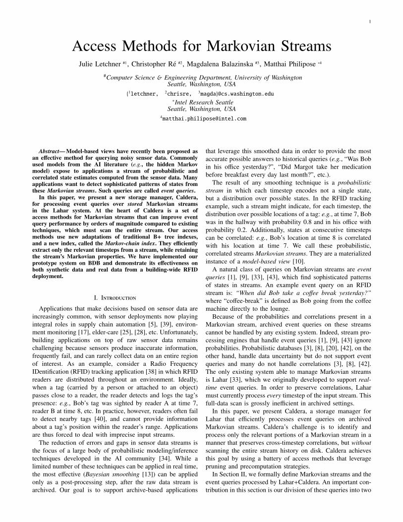
Fig. 1. The flow of data in Caldera. Raw sensor data is first smoothedinto Markovian streams and archived on disk. Caldera processes application-specified Regular event queries on these archived Markovian streams andreturns the result tuples < t, p > specifying the probability p that the queryis satisfied at time t, for each timestep in the stream.
classes, which we call fixed-length and variable-length queries.We identify the challenges involved in processing each. Ouralgorithmic contributions are access methods optimized foreach query class. Specifically, these contributions include:
1) An access method optimized for fixed-length queries,based upon a novel adaptation of standard indexingtechniques (Section III-A).
2) A top-k optimization for fixed-length queries. This secondaccess method exploits insights about the structure ofMarkovian event probabilities to adapt standard top-k pruning techniques to Markovian stream data, usingstandard B+ trees (Section III-B).
3) A novel index structure (the Markov chain index) andassociated access method for variable-length queries, forwhich standard indexing is insufficient (Section III-C).
4) A discussion of practical issues relating to our threeaccess methods, including predicate evaluation and acomparison of physical disk layouts (Section III-D).
In Section IV we demonstrate the efficiency of our four ac-cess methods on both real and synthetic data. We show on realdata that Caldera’s access methods deliver speedups of up totwo orders of magnitude over a naıve stream scan. We then usesynthetic data to push beyond the limitations of our real datasetand confirm that our algorithms continue to provide similarspeedups under a wider variety of stream conditions. Finally,we identify unique characteristics of location-based Markovianstreams, and we discuss the impact of these characteristicsupon access method performance, disk layout choice, and thequality of a heuristic-based, approximate access method.
II. PIn this section we give an overview of the queries and data
processed by Lahar+Caldera (see Figure 1). We first sketchone of the many processes by which Markovian streams canbe generated from sensor data. We then describe event queriesover Markovian streams and outline the major challenges toprocessing them in an archived setting.
A. Hidden Markov Models and Markovian Streams
Consider again the example scenario in which RFID readerstrack Bob’s location as he moves throughout a building.Because RFID readers are placed at discrete locations andbecause of noise and interference, the raw RFID streamrepresenting Bob’s location contains errors and gaps. Often,however, a system can use probabilistic inference to reduceerrors and provide location estimates during times for whichno sensor data is available.
Many of the methods for inferring these location estimatesrely upon a simple and commonly-used graphical model calleda hidden Markov model (HMM) [29]. The HMM is designedto infer a sequence of hidden state values (e.g. Bob’s locations)from a sequence of observations (e.g. RFID tag reads). TheHMM incorporates both physical constraints (e.g. a personcannot go directly from office O1 to office O2, since this wouldinvolve walking through a wall; a tag is most likely no morethan 5 feet from the RFID antenna detecting it, since antennaranges are small) as well as statistical likelihoods (e.g. it ismore likely that Bob will enter his own office, rather than hisneighbor’s). The construction of this model is orthogonal toCaldera’s contribution, so we do not describe it here, but referthe reader instead to Rabiner’s excellent tutorial [29].
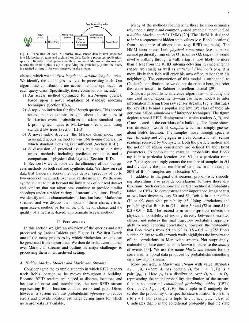
Standard probabilistic inference algorithms—including theone used in our experiments—can use these models to inferinformation missing from raw sensor streams. Fig. 2 illustratesthe key idea behind a popular and intuitive class of these al-gorithms called sample-based inference techniques. The figuredepicts a small RFID deployment in which readers A, B, andC are located in the corridors of a building. The figure showstwo timesteps’ worth of samples, which are simply guessesabout Bob’s location. The samples move through space ateach timestep and congregate in areas consistent with sensorreadings received by the system. Both the particle motion andthe notion of sensor consistency are defined by the HMMparameters. To compute the marginal probability that Bob’stag is in a particular location, e.g. H1, at a particular time,e.g. 7, the system simply counts the number of samples in H1and divides by the total number of samples. In this example,80% of Bob’s samples are in location H1.
In addition to marginal distributions, probabilistic smooth-ing algorithms also provide correlations between these dis-tributions. Such correlations are called conditional probabilitytables, or CPTs. To demonstrate their importance, imagine thatat two later timesteps, say 50 and 51, Bob is in either officeO1 or O2, each with probability 0.5. Using correlations, theprobability that Bob is in O1 at time 50 and O2 at time 51 is0.5 ∗ 0.0 = 0.0. The second term in this product reflects thephysical impossibility of moving directly between these twooffices, and reduces the final trajectory probability appropri-ately to zero. Ignoring correlations, however, the probabilitythat Bob moves from O1 to O2 is 0.5 ∗ 0.5 = 0.25! Bob’ssudden ability to walk through walls highlights the importanceof the correlations in Markovian streams. Not surprisingly,maintaining these correlations is known to increase the qualityof events [33]. We use the name Markovian stream for thecorrelated, temporal data produced by probabilistic smoothingon a raw input stream.
More precisely, a Markovian stream with value attributesA1, . . . , Ak (where Ai has domain Di for i ∈ [1, k]) is apair (p0, C). Here p0 is a distribution over D1 × · · · × Dk,representing the initial probability distribution of the stream;C is a sequence of conditional probability tables (CPTs)C(A1, . . . , Ak, A′1, . . . , A
′k,T, P). Each tuple in C uniquely de-
scribes the probability of a specific state transition from timet to t + 1. For example, a tuple (a1, . . . , ak, a′1, ..., a
′k, t, p) in
C indicates that p is the conditional probability that the state
3
O1
O5
H1 H2 H3
O2 O3
BO4
H2H1 H3
O1 O2 O3
O5BO4
Bob 7 O1 0.05
Bob 7 H1 0.80Bob 7 H2 0.15
p(l)t ltagBob 7 8 H1 H1 0.625 Bob 7 8 H1 H2 0.250Bob 7 8 H1 O1 0.125Bob 7 8 H1 O2 0.000Bob 7 8 H2 H1 0.000Bob 7 8 H2 H2 0.666Bob 7 8 H2 O1 0.000Bob 7 8 H2 O2 0.333Bob 7 8 O1 H1 0.000Bob 7 8 O1 H2 0.000Bob 7 8 O1 O1 1.000Bob 7 8 O1 O2 0.000
t t! l l! p(l!|l)tag
p(l)t ltag
Bob 8 O1 0.15
Bob 8 H1 0.50Bob 8 H2 0.30
Bob 8 O2 0.05
(b1)
(b2) (c)
(a1)
(a2)
A
A
C
C
Hallway location
Officelocations
RFIDantenna
O1
Fig. 2. (a) A sample-based distribution over Bob’s location at time 7 (a1) when antenna A detects Bob, and at the next time 8 (a2), when Bob is undetected.(b) The marginal distributions computed from the samples, for times 7 (b1) and 8 (b2) respectively. (c) The correlations between times 7 and 8.
of the stream is (A1 = a′1, . . . , Ak = a′k) at time t + 1, giventhat the state at time t was (A1 = a1, . . . , Ak = ak). The setof tuples sharing a value of T = t together define the entirestream transition (CPT) between t and t + 1. For a full formalsemantic, see Re et al. [33].
For performance reasons, Caldera explicitly stores themarginal distributions over the stream state at each timestep,even though they are derivable from (p0, C). Figures 2(b) and2(c) show the relational representation of a Markovian streamin which the single attribute A1 represents Bob’s location. Tofurther improve performance, zero-valued distribution entries(e.g. H3 at timesteps 7 and 8 in Figure 2) are not explicitlystored. Such values occur when inference is sample-based, orwhen very small distribution entries are pruned to zero.
B. Regular Queries on Markovian StreamsStreams lend themselves naturally to event queries [9],
which ask questions about sequences of states. An exampleevent query is, “When did Bob enter his office (300)?”.In this paper, we look at a subset of event queries calledRegular queries [33]. These queries are analogous to regularexpressions, or equivalently NFAs. An example Regular queryis shown in Figure 3(a). This query is satisfied when Bob isfirst in a Hallway, and then in Office300 in the next timestep.Regular queries comprise only linear NFAs, which means thatthe directed automaton edges form a total order.
Regular query NFAs differ from standard NFAs in that theytransition when predicates on the input stream are satisfied,instead of on static alphabet symbols. For example, the NFAin Fig. 3(a) transitions from the start state to state S 0 on inputtimesteps in which Bob’s location is a hallway (many locationsmight satisfy this predicate). If Bob’s location is not a hallway,then this transition is not possible and the automaton dies.
We define a predicate here as a Boolean function onstream attributes. For example, the Hallway predicate re-
(a)
S0 S1Hallway Office300
Entered-Office Query: (Hallway, Office300)
S0 S1Hallway Coffee Room
¬ Coffee Room
(b)
Coffee-Break Query: (Hallway, ¬CoffeeRoom*, CoffeeRoom)
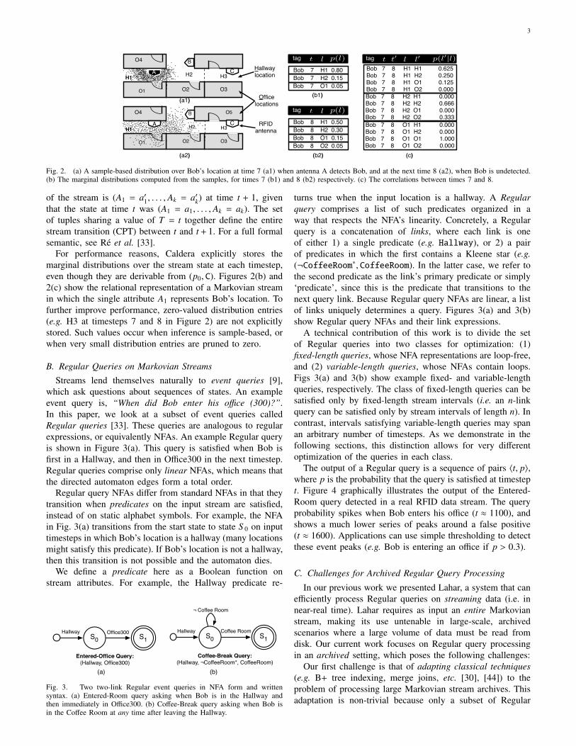
Fig. 3. Two two-link Regular event queries in NFA form and writtensyntax. (a) Entered-Room query asking when Bob is in the Hallway andthen immediately in Office300. (b) Coffee-Break query asking when Bob isin the Coffee Room at any time after leaving the Hallway.
turns true when the input location is a hallway. A Regularquery comprises a list of such predicates organized in away that respects the NFA’s linearity. Concretely, a Regularquery is a concatenation of links, where each link is oneof either 1) a single predicate (e.g. Hallway), or 2) a pairof predicates in which the first contains a Kleene star (e.g.(¬CoffeeRoom∗, CoffeeRoom). In the latter case, we refer tothe second predicate as the link’s primary predicate or simply‘predicate’, since this is the predicate that transitions to thenext query link. Because Regular query NFAs are linear, a listof links uniquely determines a query. Figures 3(a) and 3(b)show Regular query NFAs and their link expressions.
A technical contribution of this work is to divide the setof Regular queries into two classes for optimization: (1)fixed-length queries, whose NFA representations are loop-free,and (2) variable-length queries, whose NFAs contain loops.Figs 3(a) and 3(b) show example fixed- and variable-lengthqueries, respectively. The class of fixed-length queries can besatisfied only by fixed-length stream intervals (i.e. an n-linkquery can be satisfied only by stream intervals of length n). Incontrast, intervals satisfying variable-length queries may spanan arbitrary number of timesteps. As we demonstrate in thefollowing sections, this distinction allows for very differentoptimization of the queries in each class.
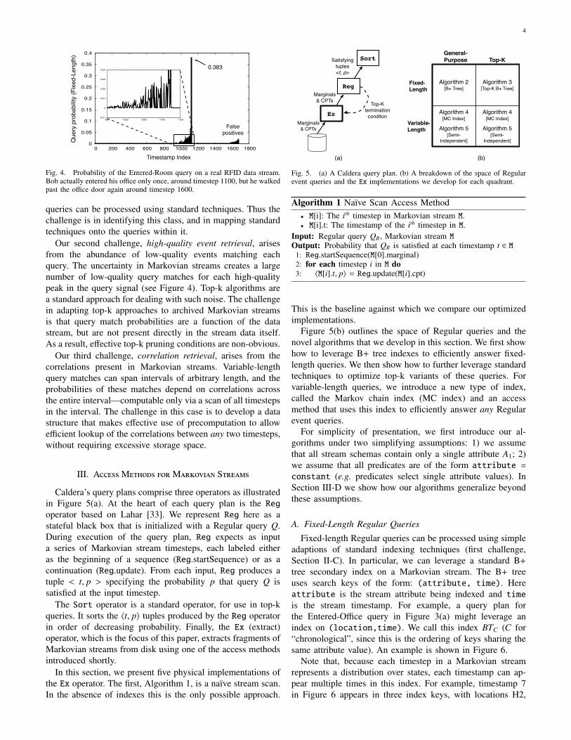
The output of a Regular query is a sequence of pairs 〈t, p〉,where p is the probability that the query is satisfied at timestept. Figure 4 graphically illustrates the output of the Entered-Room query detected in a real RFID data stream. The queryprobability spikes when Bob enters his office (t ≈ 1100), andshows a much lower series of peaks around a false positive(t ≈ 1600). Applications can use simple thresholding to detectthese event peaks (e.g. Bob is entering an office if p > 0.3).
C. Challenges for Archived Regular Query Processing
In our previous work we presented Lahar, a system that canefficiently process Regular queries on streaming data (i.e. innear-real time). Lahar requires as input an entire Markovianstream, making its use untenable in large-scale, archivedscenarios where a large volume of data must be read fromdisk. Our current work focuses on Regular query processingin an archived setting, which poses the following challenges:
Our first challenge is that of adapting classical techniques(e.g. B+ tree indexing, merge joins, etc. [30], [44]) to theproblem of processing large Markovian stream archives. Thisadaptation is non-trivial because only a subset of Regular
4
0
0.05
0.1
0.15
0.2
0.25
0.3
0.35
0.4
0 200 400 600 800 1000 1200 1400 1600 1800
Query
Pro
babili
ty (
NE
XT
sem
antic
s)
Timestamp (seconds)
Entered-Room.probs
-0.01
0
0.01
0.02
0.03
0.04
950 1000 1050 1100 1150
Que
ry p
roba
bility
(Fixe
d-Le
ngth
)
Timestamp Index
0.383
False positives
Fig. 4. Probability of the Entered-Room query on a real RFID data stream.Bob actually entered his office only once, around timestep 1100, but he walkedpast the office door again around timestep 1600.
queries can be processed using standard techniques. Thus thechallenge is in identifying this class, and in mapping standardtechniques onto the queries within it.
Our second challenge, high-quality event retrieval, arisesfrom the abundance of low-quality events matching eachquery. The uncertainty in Markovian streams creates a largenumber of low-quality query matches for each high-qualitypeak in the query signal (see Figure 4). Top-k algorithms area standard approach for dealing with such noise. The challengein adapting top-k approaches to archived Markovian streamsis that query match probabilities are a function of the datastream, but are not present directly in the stream data itself.As a result, effective top-k pruning conditions are non-obvious.
Our third challenge, correlation retrieval, arises from thecorrelations present in Markovian streams. Variable-lengthquery matches can span intervals of arbitrary length, and theprobabilities of these matches depend on correlations acrossthe entire interval—computable only via a scan of all timestepsin the interval. The challenge in this case is to develop a datastructure that makes effective use of precomputation to allowefficient lookup of the correlations between any two timesteps,without requiring excessive storage space.
III. AM M S
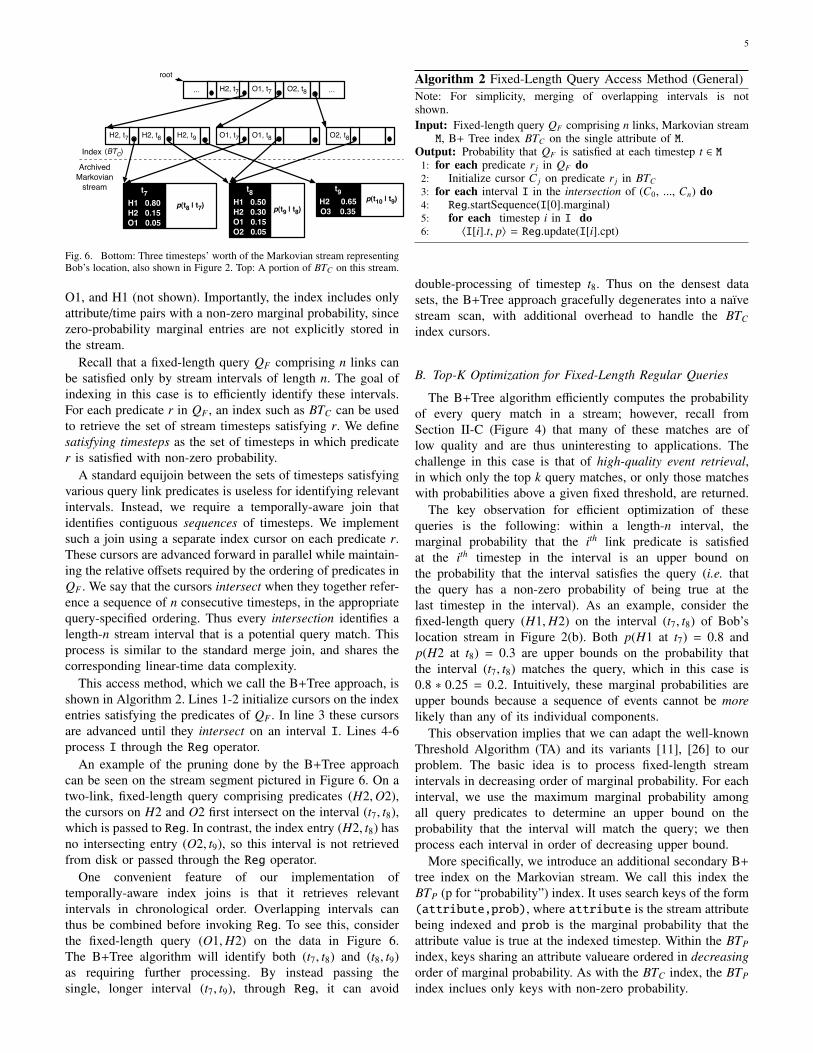
Caldera’s query plans comprise three operators as illustratedin Figure 5(a). At the heart of each query plan is the Regoperator based on Lahar [33]. We represent Reg here as astateful black box that is initialized with a Regular query Q.During execution of the query plan, Reg expects as inputa series of Markovian stream timesteps, each labeled eitheras the beginning of a sequence (Reg.startSequence) or as acontinuation (Reg.update). From each input, Reg produces atuple < t, p > specifying the probability p that query Q issatisfied at the input timestep.
The Sort operator is a standard operator, for use in top-kqueries. It sorts the 〈t, p〉 tuples produced by the Reg operatorin order of decreasing probability. Finally, the Ex (extract)operator, which is the focus of this paper, extracts fragments ofMarkovian streams from disk using one of the access methodsintroduced shortly.
In this section, we present five physical implementations ofthe Ex operator. The first, Algorithm 1, is a naıve stream scan.In the absence of indexes this is the only possible approach.
Algorithm 2[B+ Tree]
Algorithm 3[Top-K B+ Tree]
Algorithm 4[MC Index]
Algorithm 5[Semi-
Independent]
Algorithm 4[MC Index]
Algorithm 5[Semi-
Independent]
Fixed-Length
Variable-Length
General-Purpose Top-K
(b)
Ex
Reg
Sort
Top-Ktermination
conditonMarginals
& CPTs
Marginals& CPTs
Satisfyingtuples <t, p>
(a)
Fig. 5. (a) A Caldera query plan. (b) A breakdown of the space of Regularevent queries and the Ex implementations we develop for each quadrant.
Algorithm 1 Naıve Scan Access Method• M[i]: The ith timestep in Markovian stream M.• M[i].t: The timestamp of the ith timestep in M.
Input: Regular query QR, Markovian stream MOutput: Probability that QR is satisfied at each timestamp t ∈ M
1: Reg.startSequence(M[0].marginal)2: for each timestep i in M do3: 〈M[i].t, p〉 = Reg.update(M[i].cpt)
This is the baseline against which we compare our optimizedimplementations.
Figure 5(b) outlines the space of Regular queries and thenovel algorithms that we develop in this section. We first showhow to leverage B+ tree indexes to efficiently answer fixed-length queries. We then show how to further leverage standardtechniques to optimize top-k variants of these queries. Forvariable-length queries, we introduce a new type of index,called the Markov chain index (MC index) and an accessmethod that uses this index to efficiently answer any Regularevent queries.
For simplicity of presentation, we first introduce our al-gorithms under two simplifying assumptions: 1) we assumethat all stream schemas contain only a single attribute A1; 2)we assume that all predicates are of the form attribute =constant (e.g. predicates select single attribute values). InSection III-D we show how our algorithms generalize beyondthese assumptions.
A. Fixed-Length Regular Queries
Fixed-length Regular queries can be processed using simpleadaptions of standard indexing techniques (first challenge,Section II-C). In particular, we can leverage a standard B+
tree secondary index on a Markovian stream. The B+ treeuses search keys of the form: (attribute, time). Hereattribute is the stream attribute being indexed and timeis the stream timestamp. For example, a query plan forthe Entered-Office query in Figure 3(a) might leverage anindex on (location,time). We call this index BTC (C for“chronological”, since this is the ordering of keys sharing thesame attribute value). An example is shown in Figure 6.
Note that, because each timestep in a Markovian streamrepresents a distribution over states, each timestamp can ap-pear multiple times in this index. For example, timestamp 7in Figure 6 appears in three index keys, with locations H2,
5
H2, t7 H2, t8 H2, t9 O1, t7 O1, t8 O2, t8
t8H1 0.50H2 0.30O1 0.15O2 0.05
p(t9 | t8)
H2, t7 O1, t7 O2, t8...
t9H2 0.65O3 0.35
p(t10 | t9)
...
t7H1 0.80H2 0.15O1 0.05
p(t8 | t7)
Index
ArchivedMarkovian
stream
root
(BTC)
Fig. 6. Bottom: Three timesteps’ worth of the Markovian stream representingBob’s location, also shown in Figure 2. Top: A portion of BTC on this stream.
O1, and H1 (not shown). Importantly, the index includes onlyattribute/time pairs with a non-zero marginal probability, sincezero-probability marginal entries are not explicitly stored inthe stream.
Recall that a fixed-length query QF comprising n links canbe satisfied only by stream intervals of length n. The goal ofindexing in this case is to efficiently identify these intervals.For each predicate r in QF , an index such as BTC can be usedto retrieve the set of stream timesteps satisfying r. We definesatisfying timesteps as the set of timesteps in which predicater is satisfied with non-zero probability.
A standard equijoin between the sets of timesteps satisfyingvarious query link predicates is useless for identifying relevantintervals. Instead, we require a temporally-aware join thatidentifies contiguous sequences of timesteps. We implementsuch a join using a separate index cursor on each predicate r.These cursors are advanced forward in parallel while maintain-ing the relative offsets required by the ordering of predicates inQF . We say that the cursors intersect when they together refer-ence a sequence of n consecutive timesteps, in the appropriatequery-specified ordering. Thus every intersection identifies alength-n stream interval that is a potential query match. Thisprocess is similar to the standard merge join, and shares thecorresponding linear-time data complexity.
This access method, which we call the B+Tree approach, isshown in Algorithm 2. Lines 1-2 initialize cursors on the indexentries satisfying the predicates of QF . In line 3 these cursorsare advanced until they intersect on an interval I. Lines 4-6process I through the Reg operator.
An example of the pruning done by the B+Tree approachcan be seen on the stream segment pictured in Figure 6. On atwo-link, fixed-length query comprising predicates (H2,O2),the cursors on H2 and O2 first intersect on the interval (t7, t8),which is passed to Reg. In contrast, the index entry (H2, t8) hasno intersecting entry (O2, t9), so this interval is not retrievedfrom disk or passed through the Reg operator.
One convenient feature of our implementation oftemporally-aware index joins is that it retrieves relevantintervals in chronological order. Overlapping intervals canthus be combined before invoking Reg. To see this, considerthe fixed-length query (O1,H2) on the data in Figure 6.The B+Tree algorithm will identify both (t7, t8) and (t8, t9)as requiring further processing. By instead passing thesingle, longer interval (t7, t9), through Reg, it can avoid
Algorithm 2 Fixed-Length Query Access Method (General)Note: For simplicity, merging of overlapping intervals is notshown.Input: Fixed-length query QF comprising n links, Markovian streamM, B+ Tree index BTC on the single attribute of M.
Output: Probability that QF is satisfied at each timestep t ∈ M1: for each predicate r j in QF do2: Initialize cursor C j on predicate r j in BTC3: for each interval I in the intersection of (C0, ..., Cn) do4: Reg.startSequence(I[0].marginal)5: for each timestep i in I do6: 〈I[i].t, p〉 = Reg.update(I[i].cpt)
double-processing of timestep t8. Thus on the densest datasets, the B+Tree approach gracefully degenerates into a naıvestream scan, with additional overhead to handle the BTC
index cursors.
B. Top-K Optimization for Fixed-Length Regular Queries
The B+Tree algorithm efficiently computes the probabilityof every query match in a stream; however, recall fromSection II-C (Figure 4) that many of these matches are oflow quality and are thus uninteresting to applications. Thechallenge in this case is that of high-quality event retrieval,in which only the top k query matches, or only those matcheswith probabilities above a given fixed threshold, are returned.
The key observation for efficient optimization of thesequeries is the following: within a length-n interval, themarginal probability that the ith link predicate is satisfiedat the ith timestep in the interval is an upper bound onthe probability that the interval satisfies the query (i.e. thatthe query has a non-zero probability of being true at thelast timestep in the interval). As an example, consider thefixed-length query (H1,H2) on the interval (t7, t8) of Bob’slocation stream in Figure 2(b). Both p(H1 at t7) = 0.8 andp(H2 at t8) = 0.3 are upper bounds on the probability thatthe interval (t7, t8) matches the query, which in this case is0.8 ∗ 0.25 = 0.2. Intuitively, these marginal probabilities areupper bounds because a sequence of events cannot be morelikely than any of its individual components.
This observation implies that we can adapt the well-knownThreshold Algorithm (TA) and its variants [11], [26] to ourproblem. The basic idea is to process fixed-length streamintervals in decreasing order of marginal probability. For eachinterval, we use the maximum marginal probability amongall query predicates to determine an upper bound on theprobability that the interval will match the query; we thenprocess each interval in order of decreasing upper bound.
More specifically, we introduce an additional secondary B+
tree index on the Markovian stream. We call this index theBTP (p for “probability”) index. It uses search keys of the form(attribute,prob), where attribute is the stream attributebeing indexed and prob is the marginal probability that theattribute value is true at the indexed timestep. Within the BTP
index, keys sharing an attribute valueare ordered in decreasingorder of marginal probability. As with the BTC index, the BTP
index inclues only keys with non-zero probability.
6
Algorithm 3 Fixed-Length Query Access Method (Top-K)Input: Fixed-length query QF comprising n links, Markovian streamM, B+ Tree index BTP on the single attribute of M, and k
Output: Top k timesteps at which QF is satisfied in M.1: currTopK.initializeEmpty2: for each predicate r j in QF do3: Initialize cursor C j on predicate r j in BTP4: for each timestep M[t] w/ max prob. referenced by any C j do5: if M[t].marginal.prob(r j)<= currTopK.min then6: Terminate7: I = {M[t − j], ..., M[t − j + n]}8: if I[l].marginal.prob(rl)> currTopK.min, ∀ 0 ≤ l < n then9: Reg.startSequence(I[0].marginal)
10: for each i in I do11: 〈I[i].t, p〉 = Reg.update(I[i].cpt)12: currTopK.evaluate(p)
Algorithm 3 outlines an access method (the top-k B+Treeapproach) that leverages the BTP index and the TA techniqueto efficiently process top-k queries. After initialization (lines 1-3), the algorithm scans in parallel all leaves of the B+ tree thatmatch the different query predicates, returning the entry M[t]with the highest remaining marginal probability (line 4). Thealgorithm terminates when the maximum marginal probabilityof all remaining index entries (e.g. the marginal probability ofpredicate r j in timestep M[t]) is below the probability of all kof the current best query matches (lines 5-6). If this conditionis not met, the marginal probability of each predicate in theinterval I is examined (lines 7-8). If none of these is lowenough to prune the interval, the interval is processed throughthe Reg operator (lines 9-12) and the resulting probability isincorporated into the top k matches if appropriate.
As mentioned above, the marginal probability of each pred-icate in a length-n interval is only an upper bound on the prob-ability that the interval matches the query; the actual matchprobability may be much lower or even zero. In data where thisis common, the top-k B+Tree algorithm has little opportunityfor pruning, and the B+Tree implementation of Ex based onthe BTC index, followed by a sort on the output tuples, willoften outperform the top-k B+Tree approach because of itsability to combine the processing of overlapping intervals.The top-k approach, by contrast, significantly outperforms thestandard B+Tree approach on queries with clear peaks, such asthat shown in Figure 3(b). We further explore the relationshipbetween these two algorithms in our evaluation (Section IV).
C. Variable-Length Regular Queries
The fixed-length access methods in the previous sectionare inapplicable to variable-length queries, because variable-length queries can be satisfied by stream intervals of arbitrarylength. A full stream scan can be avoided in this case using thefollowing insight: while query match intervals may be arbitrar-ily long, generally only a small number of timesteps in eachinterval contain data relevant to the query (i.e., satisfy at leastone query predicate with non-zero probability). Furthermore,the query NFA changes state only on these relevant inputs. Infact, the “irrelevant” intermediate timesteps require processingonly because together they contain the correlation informationrelating each relevant timestep to the next. Thus we arrive at
p(t2 | t1)t1 t2 t3 t4 t5t0 p(t1 | t0) p(t3 | t2) p(t4 | t3) p(t5 | t4)
p(t2 | t0) p(t4 | t2)
p(t4 | t0) ...
...
i=0
i=1
i=2
p(t5 | t0) = p(t1 | t0)p(t2 | t1)p(t3 | t2)p(t4 | t3)p(t5 | t4)
= p(t4 | t0)p(t5 | t4)
≈ p(t5)
Exact: requires scan of raw data (5 conditionals of bottom row)
Exact: requires O(log n) lookups in the MC index (shaded index conditionals)
Independence assumption: requires lookup of a single marginal (t5)
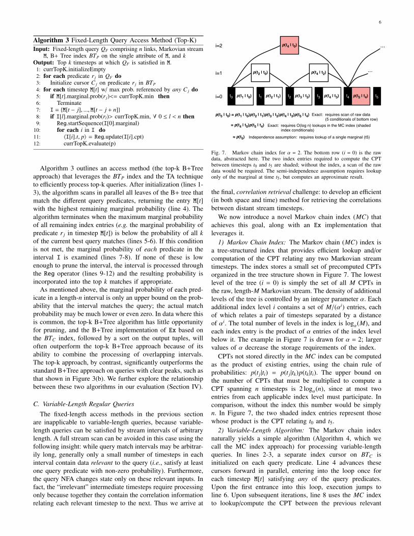
Fig. 7. Markov chain index for α = 2. The bottom row (i = 0) is the rawdata, abstracted here. The two index entries required to compute the CPTbetween timesteps t0 and t5 are shaded; without the index, a scan of the rawdata would be required. The semi-independence assumption requires lookuponly of the marginal at time t5, but computes an approximate result.
the final, correlation retrieval challenge: to develop an efficient(in both space and time) method for retrieving the correlationsbetween distant stream timesteps.
We now introduce a novel Markov chain index (MC) thatachieves this goal, along with an Ex implementation thatleverages it.
1) Markov Chain Index: The Markov chain (MC) index isa tree-structured index that provides efficient lookup and/orcomputation of the CPT relating any two Markovian streamtimesteps. The index stores a small set of precomputed CPTsorganized in the tree structure shown in Figure 7. The lowestlevel of the tree (i = 0) is simply the set of all M CPTs inthe raw, length-M Markovian stream. The density of additionallevels of the tree is controlled by an integer parameter α. Eachadditional index level i contains a set of M/(αi) entries, eachof which relates a pair of timesteps separated by a distanceof αi. The total number of levels in the index is logα(M), andeach index entry is the product of α entries of the index levelbelow it. The example in Figure 7 is drawn for α = 2; largervalues of α decrease the storage requirements of the index.
CPTs not stored directly in the MC index can be computedas the product of existing entries, using the chain rule ofprobabilities: p(t j|ti) = p(t j|tk)p(tk |ti). The upper bound onthe number of CPTs that must be multiplied to compute aCPT spanning n timesteps is 2 logα(n), since at most twoentries from each applicable index level must participate. Incomparison, without the index this number would be simplyn. In Figure 7, the two shaded index entries represent thosewhose product is the CPT relating t0 and t5.
2) Variable-Length Algorithm: The Markov chain indexnaturally yields a simple algorithm (Algorithm 4, which wecall the MC index approach) for processing variable-lengthqueries. In lines 2-3, a separate index cursor on BTC isinitialized on each query predicate. Line 4 advances thesecursors forward in parallel, entering into the loop once foreach timestep M[t] satisfying any of the query predicates.Upon the first entrance into this loop, execution jumps toline 6. Upon subsequent iterations, line 8 uses the MC indexto lookup/compute the CPT between the previous relevant
7
Algorithm 4 Variable-Length Query Access Method (MCIndex)Input: Variable-length query QV comprising n links, Markovian
stream M, B+ Tree index BTC on the single attribute of M, Markovchain index MC
Output: Probability that Qv is satisfied at each timestep t ∈ M1: tprev = Ø;2: for each predicate r j in QV do3: Initialize cursor C j on predicate r j in BTC4: for each timestep M[t] referenced by any C j do5: if tprev == Ø then6: Reg.startSequence(M[t].marginal)7: else8: cpt = MC.computeCPT(tprev, t)9: 〈M[t].t, p〉 = Reg.update(cpt)
10: tprev = t
timestep (tprev) and the current one (t). In line 9 this CPTis used to update the Reg operator. In this way the algorithmperforms a single conceptual pass over the entire stream, butleverages the MC index to avoid retrieving large spans ofirrelevant data from disk.
When a variable-length query contains loop predicates thatare not negations of non-loop predicates (e.g. (O1,H1∗,O2)),the MC index and algorithm as presented above appear in-sufficient. In this case, the large stream intervals requiringsummarization are not those containing irrelevant data, butinstead are those that continuously satisfy the query looppredicate (H1 in the example of the previous sentence). Theseconditionals are not present in the MC index as describedabove; however, they can be captured for a given predicate(e.g. H1) in a separate instance of the MC index whose entriesare conditioned on satisfaction of the predicate. The detailsof the index construction and associated access method areextremely similar to those presented for the general case, andwe omit them due to space limitations.
D. Practical Details
In this section we address several practical details whichuntil this point have been abstracted away or simplified forthe sake of presentation.
1) Indexing Predicates: Thus far we have assumed that allquery predicates are expressed as trivial equality selections ona single stream attribute. However, Caldera can also supportmulti-attribute schemas and more sophisticated predicates.Caldera is designed to work with a star schema, analogouslyto data warehouses: the Markovian stream corresponds to the(multi-attribute) facts table, while separate dimension tablesprovide extra information about stream attributes. Consideras an example the RFID-derived Markovian stream withschema (tagID,locationID,time,probability). Addi-tional information about individual locationIDs could bestored in a dimension table called LocationType, with schema(locationID,locationType) and tuples of the form(“Room300”, “CoffeeRoom”), (“HallwaySegment3”, “Hall-way”), etc..
As in a data warehouse, Caldera supports join indexesbetween the stream relation M and one or more dimension
relations D. Conceptually, the join index extends the tuples inM with the attributes of D and indexes the resulting relation. Inpractice, we create the index directly on M without modifyingit (e.g., the BTC and BTP indexes).
When the probability of a predicate Pi at a particulartimestep t is required (e.g., to create the index entries ofBTP for time t), it is computed by summing the marginalprobabilities of all tuples whose attribute values satisfy Pi
at t; this construction is valid because tuples with the sametimestamp are disjoint. Conditional predicate probabilities aresimilarly combined via weighted averages.
In the case where a Markovian stream is defined overmultiple attributes, it is possible that indexes exist on only asubset of these attributes. Our fixed-length access methods cansimply use whatever indexes are available. Our variable-lengthaccess method, however, requires indexes on all attributesinvolved in any of the query predicates. If any of these indexesis unavailable, a naıve full data scan is the only processingoption supported by Caldera.
Finally, with the exception of the top-k implementation, allaccess methods support both equality and range predicates.
2) Physical Schema: Markovian stream archives are mostlogically partitioned by stream, since Regular queries are eachdefined over a single stream (e.g. over Bob’s location or Sue’slocation, but not both at the same time). Within a Markovianstream, we choose to order data chronologically since the Regoperator needs to process data in that order; however, severaldisk layouts fulfill this constraint.
Separated Layout: In this layout, the marginal and con-ditional sequences are each laid out chronologically, but inseparate locations (e.g. separate files). This layout optimizesfor situations where most accesses are made to one sequenceor the other, but not to both. Indexes on this layout areconstructed separately for each sequence.
Co-Clustered Layout: In this layout, the marginal and con-ditional sequences are interleaved such that the marginal andconditional tuples representing a single timestep are placedtogether on disk, immediately before the marginal/conditionaltuples representing the chronologically-next timestep. Thisminimizes access cost for operations requiring access to boththe marginal and conditional data for most timesteps. Indexeson this layout are constructed as shown in Figure 6.
While the optimal layout is workload-dependent, we findin Section IV that for common queries on an RFID-derivedlocation stream, the separated layout yields faster performance.
3) Variable-Length Algorithm (Approximate): While ourMC index algorithm provides applications with an elegantspace/time tradeoff, we acknowledge that some disk-hungryor time-critical applications may not be satisfied by any pointin this tradeoff space. For these applications we providea final access method that is both more efficient than thesemi-independent approach, and does not require use of theMC index; however, it returns only approximate results. Wecall this algorithm the semi-independent approach because itassumes independence between some—but not all—timestepsin a Markovian stream.
Algorithm 5 outlines the semi-independent approach whichis similar to Algorithm 4 (we again assume a single-attribute
8
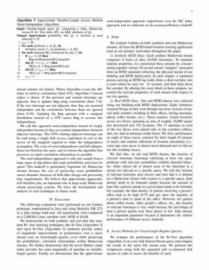
Algorithm 5 Approximate Variable-Length Access Method(Semi-Independent Algorithm)Input: Variable-length query QV comprising n links, Markovian
stream M, B+ Tree index BTC on ALL attributes of QVOutput: Approximate probability that Qv is satisfied at each
timestep t ∈ M1: tprev = Ø;2: for each predicate r j in QV do3: Initialize cursor C j on predicate r j in BTC4: for each timestep M[t] referenced by any C j do5: if tprev == Ø then6: Reg.startSequence(M[t].marginal)7: else if t == tprev + 1 then8: 〈M[t].t, p〉 = Reg.update(M[t].cpt)9: else if t > tprev + 1 then
10: 〈M[t].t, p〉 = Reg.update(M[t].marginal)11: tprev = t
stream schema, for clarity). Where Algorithm 4 uses the MCindex to retrieve correlations (lines 8-9), Algorithm 5 insteadmakes a choice: If the previous and current timesteps areadjacent, then it updates Reg using correlations (lines 7-8).If the two timesteps are not adjacent, then they are assumedindependent and the correlations between them are ignored(lines 9-10). Updating the Reg operator with a marginaldistribution instead of a CPT causes Reg to assume thisindependence.
We call this approach semi-independent instead of simplyindependent because it does not assume independence betweenadjacent timesteps. The CPTs relating adjacent timesteps canbe read using a single disk access, equivalent in cost to theaccess of the marginal required to make the independenceassumption. The costs of semi-independence and full indepen-dence are therefore the same, and we choose the algorithm thatpreserves as much correlation information as possible.
The semi-independence approach is only one sample from alarge space of algorithms that trade probabilistic precision forspeed. This tradeoff is particularly important for Markovianstreams because the cost of preserving exact probabilitiescauses dramatic increases in both data storage and processingtime requirements. We believe that approximate approacheswill therefore play an important role in large-scale Markovianstream processing systems. We leave the development andanalysis of such techniques to future work.
IV. E
The following evaluations were performed on our Calderaprototype, implemented in Java and using Berkeley DB [27]as a data storage back-end. All experiments were conductedon a 2.00GHz Linux machine with 16GB of RAM.
We demonstrate on both synthetic and real data that stan-dard B+ tree indexing techniques (the B+Tree [Algorithm 2]and top-k B+Tree [Algorithm 3] methods) provide ordersof magnitude improvements in performance over a naıvestream scan on fixed-length queries, even while preservingthe probabilistic, correlated relationships within Markovianstreams. We further demonstrate that the novel Markov chainindex provides the same magnitudes of speedup on variable-length queries. Finally we demonstrate that the approximate
semi-independent approach outperforms even the MC indexapproach, and we elaborate on its accuracy/efficiency tradeoff.
A. Setup
We evaluate Caldera on both synthetic and real Markovianstreams, all from the RFID-based location tracking applicationused as our primary motivation throughout the paper.
1) Synthetic RFID Data: Each syntheic Markovian streamcomprises 8 hours of data (30,000 timesteps). To maintainrealistic properties, we constructed these streams by concate-nating together various 30-second stream “snippets” generatedfrom an RFID simulator reflecting the physical layout of ourbuilding and RFID deployment. In each snippet, a simulatedperson carrying an RFID tag walks down a short corridor, intoa room where he stays for 15 seconds, and then back downthe corridor. By altering the room labels in these snippets, wecontrol the relevant properties of each stream with respect toour test queries.
2) Real RFID Data: Our real RFID dataset was collectedusing our building-wide RFID deployment. Eight volunteerscarryied 58 tags as they went through one-hour versions of typ-ical daily routines (working in their offices, having meetings,taking coffee breaks, etc.). These routines visited locationsacross two floors, spanning an area of roughly 10,000 squarefeet discretized into 352 locations. The 17 antennas on eachof the two floors were placed only in the corridors (offices,labs, etc. had no antennas inside them). We show performanceon eight of these traces, selected for their length (8 minutesor more) and realistic reflection of location uncertainty (i.e.,some tags were never or almost never detected and we did notuse the resulting traces).
We find that, on our real RFID dataset, the fraction ofrelevant timesteps (timesteps satisfying at least one querypredicate with non-zero probability) exhibits bimodal behav-ior: either almost all or almost none of the timesteps in astream are relevant to a specific query. We call this fractionof relevant timesteps data density and note that it is definedon a Markovian stream with respect to a specific query. Datadensity tends to be bimodal simply because the amount oftime that a person spends in a given place tends to be bimodal.For example, the data density of queries involving a person’soffice tend to be high (0.75 and up) since the majority ofa person’s time is spent in his office. However, for queriesabout coffee rooms, other people’s offices, etc., the fractionof relevant timesteps is very small because the percentage oftime a person spends near these places is low. Data densityis an important parameter because it determines the relativeperformance of different access methods.
B. Access Methods for Fixed-Length Regular Queries
We evaluate the performance of the B+Tree algorithm(Algorithm 2) on a two-link Entered-Room query and comparethe results to the naıve full stream scan. We perform thiscomparison using both the separated and co-clustered disklayouts in order to assess the benefits of each.
9
100
1000
10000
100000
0.001 0.01 0.1 1
Tim
e (
mill
ise
co
nd
s)
Fraction of Relevant Timesteps
DiskLayoutEvaluationNEXTREGULARLogscale
10
100
1000
10000
0.001 0.01 0.1 1
Tim
e (
mill
ise
co
nd
s)
Fraction of Relevant Timesteps
Tablegrantscash.mug2Subgoals.tableNEXTlogscale
Full ScanNext Regular
TopK 1
10
100
1000
10000
100000
0.001 0.01 0.1 1
Tim
e (
mill
is)
Density
NextRegularBasicLogscaleTi
me
(milli
seco
nds)
Tim
e (m
illise
cond
s)
Tim
e (m
illise
cond
s)
Density Density Density
Full data scan (separated layout)
Full data scan (coclustered layout)
B+ Tree (coclustered layout)
B+ Tree (separated layout)
Full data scan
B+ Tree
0%
25%
50%75%
100%
(a) (b) (c)
B+ Tree Algorithm Performance Fixed-Length Methods on Real Data B+ Tree Algorithm, Varying Query Match Rate
= Query shown in Figure 4
Full ScanB+ Tree
Top-K B+ Tree
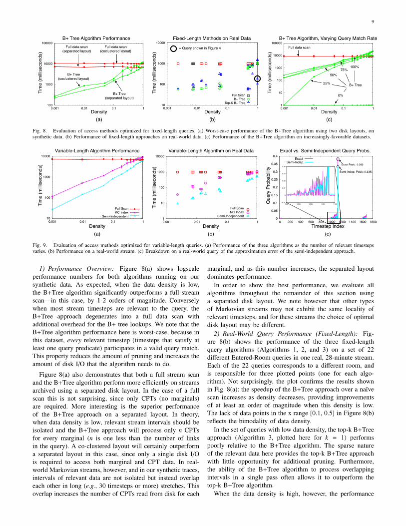
Fig. 8. Evaluation of access methods optimized for fixed-length queries. (a) Worst-case performance of the B+Tree algorithm using two disk layouts, onsynthetic data. (b) Performance of fixed-length approaches on real-world data. (c) Performance of the B+Tree algorithm on increasingly-favorable datasets.
0
0.05
0.1
0.15
0.2
0.25
0.3
0.35
0.4
0 200 400 600 800 1000 1200 1400 1600 1800
En
tere
d-R
oo
m P
rob
ab
ility
Stream Timesteps
AFTER Semantics: Exact vs. Approximate Probabilities
ExactApproximate
-0.01
0
0.01
0.02
0.03
0.04
950 1000 1050 1100 1150
Approximate Peak: 0.335
Exact Peak: 0.383
10
100
1000
10000
0.001 0.01 0.1 1
Tim
e (
mill
is)
Fraction Relevant Timesteps
MarkovVSFullScanM1.0SEPARATED
Full ScanMC Index
Indep. 1
10
100
1000
10000
0.001 0.01 0.1 1
Tim
e (
mill
iseconds)
Fraction of Relevant Timesteps
Tablegrantscash.mug2Subgoals.tableAFTERlogscale
Full ScanMC Index
Non-Adjacent Independence
Que
ry P
roba
bility
Density Density Timestep Index(a) (b) (c)
Tim
e (m
illise
cond
s)
Tim
e (m
illise
cond
s)
Variable-Length Algorithm Performance Variable-Length Algorithm on Real Data Exact vs. Semi-Independent Query Probs.
Full ScanMC Index
Semi-Independent
Full ScanMC Index
Semi-Independent
Semi-Indep.
Semi-Indep. Peak: 0.335.
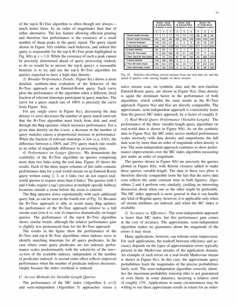
Fig. 9. Evaluation of access methods optimized for variable-length queries. (a) Performance of the three algorithms as the number of relevant timestepsvaries. (b) Performance on a real-world stream. (c) Breakdown on a real-world query of the approximation error of the semi-independent approach.
1) Performance Overview: Figure 8(a) shows logscaleperformance numbers for both algorithms running on oursynthetic data. As expected, when the data density is low,the B+Tree algorithm significantly outperforms a full streamscan—in this case, by 1-2 orders of magnitude. Converselywhen most stream timesteps are relevant to the query, theB+Tree approach degenerates into a full data scan withadditional overhead for the B+ tree lookups. We note that theB+Tree algorithm performance here is worst-case, because inthis dataset, every relevant timestep (timesteps that satisfy atleast one query predicate) participates in a valid query match.This property reduces the amount of pruning and increases theamount of disk I/O that the algorithm needs to do.
Figure 8(a) also demonstrates that both a full stream scanand the B+Tree algorithm perform more efficiently on streamsarchived using a separated disk layout. In the case of a fullscan this is not surprising, since only CPTs (no marginals)are required. More interesting is the superior performanceof the B+Tree approach on a separated layout. In theory,when data density is low, relevant stream intervals should beisolated and the B+Tree approach will process only n CPTsfor every marginal (n is one less than the number of linksin the query). A co-clustered layout will certainly outperforma separated layout in this case, since only a single disk I/Ois required to access both marginal and CPT data. In real-world Markovian streams, however, and in our synthetic traces,intervals of relevant data are not isolated but instead overlapeach other in long (e.g., 30 timesteps or more) stretches. Thisoverlap increases the number of CPTs read from disk for each
marginal, and as this number increases, the separated layoutdominates performance.
In order to show the best performance, we evaluate allalgorithms throughout the remainder of this section usinga separated disk layout. We note however that other typesof Markovian streams may not exhibit the same locality ofrelevant timesteps, and for these streams the choice of optimaldisk layout may be different.
2) Real-World Query Performance (Fixed-Length): Fig-ure 8(b) shows the performance of the three fixed-lengthquery algorithms (Algorithms 1, 2, and 3) on a set of 22different Entered-Room queries in one real, 28-minute stream.Each of the 22 queries corresponds to a different room, andis responsible for three plotted points (one for each algo-rithm). Not surprisingly, the plot confirms the results shownin Fig. 8(a): the speedup of the B+Tree approach over a naıvescan increases as density decreases, providing improvementsof at least an order of magnitude when this density is low.The lack of data points in the x range [0.1, 0.5] in Figure 8(b)reflects the bimodality of data density.
In the set of queries with low data density, the top-k B+Treeapproach (Algorithm 3, plotted here for k = 1) performspoorly relative to the B+Tree algorithm. The sparse natureof the relevant data here provides the top-k B+Tree approachwith little opportunity for additional pruning. Furthermore,the ability of the B+Tree algorithm to process overlappingintervals in a single pass often allows it to outperform thetop-k B+Tree algorithm.
When the data density is high, however, the performance
10
of the top-k B+Tree algorithm is often–though not always—much better (here, by an order of magnitude) than that ofeither alternative. The key feature allowing efficient pruningand therefore fast performance is the existence of a smallnumber of sharp peaks in the query signal. The query signalshown in Figure 3(b) exhibits such behavior, and indeed thisquery is responsible for the top-k B+Tree point highlighted inFig. 8(b) at x = 1.0. While the existence of such a peak cannotbe precisely determined ahead of query processing (indeed,to do so would be to answer the top-k query), a reasonableheuristic is to try and use the top-k B+Tree algorithm forqueries expected to have a high data density.
3) Broader Performance Trends: Figure 8(c) shows a moredetailed, synthetic-data evaluation of the behavior of theB+Tree approach on an Entered-Room query. Each curveplots the performance of the algorithm when a different, fixedfraction of relevant timesteps participate in query matches. Thecurve for a query match rate of 100% is precisely the curvefrom Figure 8(a).
For any single curve in Figure 8(c), decreasing the datadensity (x-axis) decreases the number of query match intervalsthat the B+Tree algorithm must fetch from disk and sendthrough the Reg operator, which increases performance. For agiven data density on the x-axis, a decrease in the number ofquery matches causes a proportional increase in performance.When the fraction of relevant timesteps is low (e.g. 0.01), thedifference between a 100% and 25% query match rate resultsin an order of magnitude difference in processing time.
4) Performance on Longer Queries: We demonstrate thescalability of the B+Tree algorithm on queries comprisingmore than two links using the real data. Figure 10 shows theresults. Each of the three major columns of this table containsperformance data for a real-world stream on an Entered-Roomquery written using 2, 3, or 4 links (we do not expect real-world queries to require more than 4 links). The queries with 3and 4 links require a tag’s presence at multiple specific hallwaylocations outside a room before the room is entered.
The Reg operator slows exponentially with each additionalquery link, as can be seen in the fourth row of Fig. 10. Becausethe B+Tree approach is able to avoid many Reg updates,the performance of the B+Tree approach relative to a fullstream scan (row 6 vs. row 4) improves dramatically on longerqueries. The performance of the top-k B+Tree algorithmshows similar trends, although the relative performance gainis slightly less pronounced than for the B+Tree approach.
The results in the figure show the performance of theB+Tree and top-k B+Tree algorithms when indexes serve toidentify matching timesteps for all query predicates. In thecase where some query predicates are not indexed, perfor-mance scales predominantly with the selectivity of the inter-section of the available indexes, independent of the numberof predicates indexed. A second-order effect reflects improvedperformance when the number of predicate indexes decreases,simply because the index overhead is reduced.
C. Access Methods for Variable-Length QueriesThe performance of the MC index (Algorithm 4, α=2)
and semi-independent (Algorithm 5) approaches versus a
Stream length (timesteps)
Time: B+ Tree (msec)
548 625 120626 26 11174 232 26656 75 214
# query matches
Time: MC Index (msec)
554 613 12012 1 159 67 13267 98 165
7.6 7.6 7.6458 458 4585 5 6
Time: Top-K B+ Tree (msec)
Time: Full Scan (msec)
Stream: JamesQ: Entered-Office
# Subgoals in query:
2 3 4
Stream length (minutes)
# relevant timesteps
TIme: Semi-Indep. (msec)
# query matches
Stream: SallyQ: Entered-Office
# Subgoals in query:
2 3 4
FIXED
VAR
7.7 7.7 7.7462 462 462149 194 211
145 188 188290 424 678114 156 379
2 1 132 43 1179 12 22
977 1124 30343 1 167 71 13595 366 1970
Stream: PatQ: Coffee-Room
# Subgoals in query:
2 3 4
28 28 281683 1683 168333 53 253
3 21 21187 237 90239 68 398
Fig. 10. Statistics describing several streams from our real data set, and thespeed of queries with varying lengths on these streams.
naıve stream scan, on synthetic data and the now-familiarEntered-Room query, are shown in Figure 9(a). Data densityis again the dominant factor in the performance of bothalgorithms, which exhibit the same trends as the B+Treeapproach. Figures 9(a) and 8(a) are directly comparable. Theapproximate, semi-independent approach is consistently fasterthan the precise MC index approach, by a factor of roughly 8.
1) Real-World Query Performance (Variable-Length): Theperformance of the three variable-length query algorithms onreal-world data is shown in Figure 9(b). As on the syntheticdata in Figure 9(a), the MC index access method performancescales inversely with data density and outperforms the fulldata scan by more than an order of magnitude when density islow. The semi-independent approach continues to show perfor-mance improvements over the MC index algorithm measuringjust under an order of magnitude.
The queries shown in Figure 9(b) are precisely the queriesplotted in Figure 8(b), with Kleene closures added to makethese queries variable-length. The data in these two plots istherefore directly comparable (note the fact that the naıve datascan reflects the same constant time in both figures). Algo-rithms 2 and 4 perform very similarly, yielding an interestingdiscussion about when one or the other might be preferable.The MC index approach is more general in that it can handleany kind of Regular query; however, it is applicable only whenall stream attributes are indexed, and when the MC index isavailable.
2) Accuracy vs. Efficiency: The semi-independent approachis faster than MC index, but this performance gain comesat the cost of accuracy. The approximate, semi-independentalgorithm makes no guarantees about the magnitude of theerrors it may incur.
Many applications, however, can tolerate some imprecision.For such applications, the tradeoff between efficiency and ac-curacy depends on the types of approximation errors typicallypresent in the Markovian streams of the application domain.An example of such errors on a real-world Markovian streamis shown in Figure 9(c). In this case, the approximate queryprobabilities track the magnitudes of the precise probabilitiesfairly well. The semi-independent algorithm correctly identi-fies the maximum-probability timestep (this is not guaranteedor even likely in some datasets), incurring a relative errorof roughly 13%. Applications in many circumstances may bewilling to use these approximate results in return for an order-
11
# of CPTs in the Markov Chain index on a trace of length
(in timesteps, levels 1 and up):
1796 28,796 604,793598 9598 201596256 4113 86398
1800(30 min)
28,800(8 hours)
604,800(1 week)
119 1919 4031857 928 19508
4
8
16
2
α
32
28 457 959964
(a)
Tim
e (m
illise
cond
s)
CPT Interval Length (timesteps)
(b)
0
10
20
30
40
50
60
70
80
90
100
0 5 10 15 20 25 30 35 40 45 50
Tim
e (
mill
is)
Interval Length (in timesteps)
Efficiency Gains By MC Index Level
Full Data ScanLevels 0+Levels 1+Levels 2+Levels 3+Levels 4+Levels 5+
012345
Lowest level (i) present in index:
012
3
4
∞ (= no index) (= full data scan)Lowest level present
in the MC index thatcreated each trend lineis shown near the line.
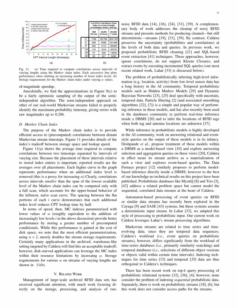
Fig. 11. (a) Time required to compute correlations across intervals ofvarying lengths using the Markov chain index. Each successive line plotsperformance when omitting an increasing number of lower index levels. (b)Storage requirements for the Markov chain index under varying α values.
of-magnitude speedup.Anecdotally, we find the approximations in Figure 9(c) to
be a fairly optimistic sampling of the output of the semi-independent algorithm. The semi-independent approach onother of our real-world Markovian streams failed to properlyidentify the maximum-probability timestep, giving errors withraw magnitudes up to 0.286.
D. Markov Chain Index
The purpose of the Markov chain index is to provideefficient access to (precomputed) correlations between distantMarkovian stream timesteps. Figure 11 provides details of theindex’s tradeoff between storage space and lookup speed.
Figure 11(a) shows the average time required to computecorrelations between two timesteps separated by intervals ofvarying size. Because the placement of these intervals relativeto stored index entries is important, reported results are theaverages over all placements. Each higher curve in the graphrepresents performance when an additional index level isremoved (this is a proxy for increasing α) Clearly, correlationsacross intervals smaller than the span of the lowest availablelevel of the Markov chain index can be computed only witha full scan, which accounts for the upper-bound behavior ofthe leftmost, naıve scan curve. The spacing between the flatportions of each i curve demonstrates that each additionalindex level reduces CPT lookup time by half.
In terms of speed, then, MC indexes parameterized withlower values of α (roughly equivalent to the addition ofincreasingly low levels i in the above discussion) provide betterperformance by storing a greater number of precomputedconditionals. While this performance is gained at the cost ofdisk space, we note that the most efficient parameterization,using α = 2, merely doubles the stream storage requirements.Certainly many applications in the archived, warehouse-likesetting targeted by Caldera will find this an acceptable tradeoff;however, disk-starved applications can leverage the MC indexwithin their resource limitations by incresaing α. Storagerequirements for various α on streams of varying lengths areshown in 11(b).
V. RWManagement of large-scale archived RFID data sets has
received significant attention, with much work focusing di-rectly on the storage, processing, and analysis of raw,
noisy RFID data [14], [16], [24], [31], [39]. A complemen-tary body of work addresses the cleanup of noisy RFIDstreams and presents methods for producing cleaned—but stilldeterministic—streams [19], [31], [39]. By contrast, Calderapreserves the uncertainty (probabilities and correlations) atthe levels of both data and queries. In previous work, weproposed probabilistic RFID cleaning [21] and SQL-basedevent extraction [41] techniques. These approaches, however,ignore correlations, do not support Kleene Closures, andextract events by executing incremental SQL queries (our mostrecent related work, Lahar [33] is discussed below).
The problem of probabilistically inferring high-level infor-mation (e.g. location, activity) from low-level sensor data hasa long history in the AI community. Temporal probabilisticmodels such as Hidden Markov Models [29] and DynamicBayesian Networks [23], [25] deal specifically with uncertain,temporal data. Particle filtering [2] (and associated smoothingalgorithms [22], [7]) is a simple and popular way of perform-ing inference in these models, and has also recently been usedin the databases community to perform real-time inferenceinside a DBMS [20] and to infer the locations of RFID tagswhen both tag and antenna locations are unknown [37].
While inference in probabilistic models is highly developedin the AI community, work on answering relational and event-style queries on the output of these models is in its infancy.Deshpande et al., propose treatment of these models withina DBMS as a model-based view [10] and explore answeringselection and aggregation queries on these views [20]; Calderain effect treats its stream archive as a materialization ofsuch a view and explores event-based queries. The DataFurnace project [12] similarly proposes to perform model-based inference directly inside a DBMS; however to the bestof our knowledge no technical results on this project have beenpublished. Probabilistic databases like MystiQ [8] and Trio [3],[42] address a related problem space but cannot model thesequential, correlated data streams at the heart of Caldera.
Automaton-based processing of event queries on RFIDor similar data streams has recently been explored in theCayuga [9] and SASE [43] systems, but these systems assumea deterministic input stream. In Lahar [33], we adapted thisstyle of processing to probabilistic input. Our current work onCaldera leverages Lahar’s stream processing algorithms.
Markovian streams are related to time series and time-evolving data, since they are temporal data sequences.Caldera’s workload (i.e., event queries on probabilisticstreams), however, differs significantly from the workload oftime-series databases (i.e., primarily similarity searching) andtemporal databases (i.e., selections of different object versionsor objects valid within certain time intervals). Indexing tech-niques for time series [15] and temporal [35] data are thusorthogonal to Caldera’s techniques.
There has been recent work on top-k query processing ofprobabilistic relational systems [32], [36], [4]; however, noneconsider the problem of indexing sequential probabilistic data.Separately, there is work on probabilistic streams [18], [6], butthis work does not consider access paths for the streams.
12
VI. C
In this paper we presented Caldera, a system for executingevent queries over archived Markovian streams. In contrastto previous systems that must process the entire Markovianstream to answer an event query, Caldera selectively processesonly relevant parts of the stream, thus achieving significantperformance gains. At the same time, Caldera preserves resultaccuracy by retaining the Markovian properties of the streamwhile skipping data.
To achieve high performance, Caldera distinguishes dif-ferent types of queries (fixed-length and variable-length). Itthen uses novel and efficient access methods specialized foreach query type. For fixed-length queries, Caldera uses noveladaptations of standard B+ tree indexes. For variable-lengthqueries, it leverages a new type of index, the MC index, toeffectively summarize unimportant parts of a stream. Addition-ally, Caldera supports top-k queries that effectively filter outnoise in query results and can also improve performance inthe case of fixed-length queries. Using synthetic and real data,we demonstrated that Caldera offers performance that can beorders magnitude better than that of a full stream scan.
Overall, effective techniques for managing noisy sensor dataare important for many applications today and we view thiswork as an important step in this direction.
A
This work was partially supported by NSF Grants IIS-0713123, IIS-0454425, and CRI-0454394. J. Letchner is sup-ported by an NSF graduate research fellowship.
R[1] J. Agrawal, Y. Diao, D. Gyllstrom, and N. Immerman. Efficient pattern
matching over event streams. In Proc. of the SIGMOD Conf., June 2008.[2] S. Arulampalam, S. Maskell, N. Gordon, and T. Clapp. A tutorial
on particle filters for on-line non-linear/non-gaussian bayesian tracking.IEEE Transactions on Signal Processing, 50(2):174–188, Feb. 2002.
[3] O. Benjelloun, A. D. Sarma, A. Halevy, and J. Widom. Uldbs: Databaseswith uncertainty and lineage. In VLDB, pages 953–964, 2006.
[4] D. Burdick, P. M. Deshpande, T. S. Jayram, R. Ramakrishnan, andS. Vaithyanathan. Olap over uncertain and imprecise data. The VLDBJournal, 16(1):123–144, 2007.
[5] Computerworld. Procter & Gamble: Wal-Mart RFID effort ef-fective. http://www.computerworld.com/action/article.do?command=viewArticleBasic&articleId=284160, Feb. 2007.
[6] G. Cormode and M. N. Garofalakis. Sketching probabilistic datastreams. In SIGMOD Conference, pages 281–292, 2007.
[7] R. G. Cowell, S. L. Lauritzen, A. P. David, and D. J. Spiegelhalter.Probabilistic Networks and Expert Systems. Springer-Verlag New York,Inc., Secaucus, NJ, USA, 1999.
[8] N. Dalvi and D. Suciu. Efficient query evaluation on probabilisticdatabases. In Prov. of the 30th VLDB Conf, 2004.
[9] A. Demers, J. Gehrke, M. Hong, M. Riedewald, and W. White. Towardsexpressive publish/subscribe systems. In Proc. of 10th EDBT Conf., Mar.2006.
[10] A. Deshpande and S. Madden. MauveDB: supporting model-based userviews in database systems. In Proc. of the SIGMOD Conf., June 2006.
[11] R. Fagin, A. Lotem, and M. Naor. Optimal aggregation algorithms formiddleware. In Proc. of the 20th PODS Conf., 2001.
[12] Garofalakis et. al. Probabilistic data management for pervasive comput-ing: The Data Furnace project. IEEE Data Engineering Bulletin, 29(1),Mar. 2006.
[13] A. Gelman, J. B. Carlin, H. S. Stern, and D. B. Rubin. Bayesian DataAnalysis. Chapman and Hall/CRC, 2003.
[14] H. Gonzalez, J. Han, X. Li, and D. Klabjan. Warehousing and analyzingmassive RFID data sets. In Proc. of the 22nd ICDE Conf., Apr. 2006.
[15] J. Han and M. Kamber. Data Mining: Concepts and Techniques. MorganKaufmann Publishers Inc., second edition, 2005.
[16] Y. Hu, S. Sundara, T. Chorma, and J. Srinivasan. Supporting RFID-baseditem tracking applications in Oracle DBMS using a bitmap datatype. InProc. of the 31st VLDB Conf., Sept. 2005.
[17] Incorporated Research Institution for Seismology (IRIS). SeismicMonitor. http://www.iris.edu/hq/.
[18] T. S. Jayram, A. McGregor, S. Muthukrishnan, and E. Vee. Estimatingstatistical aggregates on probabilistic data streams. In PODS, pages243–252, 2007.
[19] Jeffery et al. Adaptive cleaning for RFID data streams. In Proc. of the32nd VLDB Conf., Sept. 2006.
[20] B. Kanagal and A. Deshpande. Online filtering, smoothing and proba-bilistic modeling of streaming data. In Proc. of the 24th ICDE Conf.,June 2008.
[21] N. Khoussainova, M. Balazinska, and D. Suciu. Towards correctinginput data errors probabilistically using integrity constraints. In Proc.of Fifth MobiDE Workshop, June 2006.
[22] M. Klaas, M. Briers, N. de Freitas, A. Doucet, S. Maskell, and D. Lang.Fast particle smoothing: if I had a million particles. In Proc. of the 23rdICML, pages 481–488, New York, NY, USA, 2006. ACM.
[23] S. L. Lauritzen. Graphical Models. Number 17 in Oxford StatisticalScience Series. Clarendon Press, Oxford, 1996.
[24] C.-H. Lee and C.-W. Chung. Efficient storage scheme and queryprocessing for supply chain management using RFID. In Proc. of theSIGMOD Conf., June 2008.
[25] L. Liao, D. J. Patterson, D. Fox, and H. A. Kautz. Learning and inferringtransportation routines. Artif. Intell, 171(5-6):311–331, 2007.
[26] A. Marian. Evaluating top-k queries over web-accessible databases. InProc. of the 18th ICDE Conf., 2002.
[27] M. A. Olson, K. Bostic, and M. Seltzer. Berkeley db. In ATEC ’99:Proceedings of the annual conference on USENIX Annual TechnicalConference, pages 43–43, Berkeley, CA, USA, 1999. USENIX Associ-ation.
[28] M. Philipose, K. P. Fishkin, M. Perkowitz, D. J. Patterson, D. Fox,H. Kautz, and D. Hahnel. Inferring activities from interactions withobjects. IEEE Pervasive Computing, 3(4):50–57, 2004.
[29] L. R. Rabiner. A tutorial on hidden markov models and selectedapplications in speech recognition. pages 267–296, 1990.
[30] R. Ramakrishnan and J. Gehrke. Database Management Systems.McGraw-Hill Science Engineering, third edition, 2002.
[31] J. Rao, S. Doraiswamy, H. Thakkar, and L. S. Colby. A deferredcleansing method for RFID data analytics. In Proc. of the 32nd VLDBConf., Sept. 2006.
[32] C. Re, N. Dalvi, and D. Suciu. Efficient Top-k query evaluation onprobabilistic data. In ICDE, 2007.
[33] C. Re, J. Letchner, M. Balazinska, and D. Suciu. Event queries oncorrelated probabilistic streams. In Proc. of the SIGMOD Conf., June2008.
[34] S. Russell and P. Norvig. Artificial Intelligence: A Modern Approach.Prentice-Hall, Englewood Cliffs, NJ, 2nd edition edition, 2003.
[35] B. Salzberg and V. J. Tsotras. Comparison of access methods for time-evolving data. ACM Comput. Surv., 31(2):158–221, 1999.
[36] M. A. Soliman, I. F. Ilyas, and K. C.-C. Chang. Top-k query processingin uncertain databases. In ICDE, pages 896–905, 2007.
[37] T. Tran, C. Sutton, R. Cocci, Y. Nie, Y. Diao, and P. Shenoy. Probabilisticinference over RFID streams in mobile environments. Technical Report07-59, University of Massachusetts at Amherst, 2007.
[38] University of Washington. RFID Ecosystem. http://rfid.cs.washington.edu/.
[39] F. Wang and P. Liu. Temporal management of RFID data. In Proc. ofthe 31st VLDB Conf., Sept. 2005.
[40] E. Welbourne, M. Balazinska, G. Borriello, and W. Brunette. Challengesfor pervasive RFID-based infrastructures. In IEEE PERTEC 2007Workshop, Mar. 2007.
[41] E. Welbourne, N. Khoussainova, J. Letchner, Y. Li, M. Balazinska,G. Borriello, and D. Suciu. Cascadia: a system for specifying, detecting,and managing RFID events. In Proc. of the Sixth MobiSys Conf., June2008.
[42] J. Widom. Trio: A system for integrated management of data, accuracy,and lineage. In Proc of the 2nd CIDR Conf., 2005.
[43] E. Wu, Y. Diao, and S. Rizvi. High-Performance Complex EventProcessing over Streams. In Proc. of the SIGMOD Conf., June 2006.
[44] C. Zaniolo, S. Ceri, C. Faloutsos, R. T. Snodgrass, V. S. Subrahmanian,and R. Zicari. Advanced Database Systems. Morgan Kaufmann, 1997.