Embed Size (px)
Citation preview

Access to Electronic Thesis
Author: Mohd Fairusham Ghazali
Thesis title: Leak Detection Using Instantaneous Frequency Analysis
Qualification: PhD
This electronic thesis is protected by the Copyright, Designs and Patents Act 1988. No reproduction is permitted without consent of the author. It is also protected by the Creative Commons Licence allowing Attributions-Non-commercial-No derivatives. If this electronic thesis has been edited by the author it will be indicated as such on the title page and in the text.

i
LEAK DETECTION USING
INSTANTANEOUS FREQUENCY
ANALYSIS
by
Mohd Fairusham Ghazali
A dissertation submitted to the University of Sheffield for the degree of
Doctor Philosophy
May 2012
Department of Mechanical Engineering
The University of Sheffield
Mappin Street, Sheffield, S1 3JD
United Kingdom

ii
Summary Leaking pipes are a primary concern for water utilities around the globe as they
compose a major portion of losses. Contemporary interest surrounding leaks is well
documented and there is a proliferation of leak detection techniques. Although the
reasons for these leaks are well known, some of the current methods for leak detection
and location are either complicated, inaccurate and most of them are time consuming.
Transient analyses offer a plausible route towards leak detection due to their robustness
and simplicity. These approaches use the change of pressure response of the fluid in a
pipeline to identify features. The method used in the current study employ a single
pressure transducer to obtain the time domain signal of the pressure transient response
caused by a sudden opening and closing of a solenoid valve. The device used is fitted
onto a standard UK hydrant and both cause a pressure wave and acquire the pressure
history.
The work described here shows that the analysis using Hilbert transform (HT), Hilbert
Huang transform (HHT) and EMD based method is a promising tool for leak detection
and location in the pipeline network.
In the first part of the work, the analysis of instantaneous characteristics of transient
pressure signal has been calculated using HT and HHT for both simulated and
experimental data. These instantaneous properties of the signals are shown to be
capable of detecting the reflection from the features of the pipe such as leakages and
outlet. When tested with leak different locations, the processed results still show the
existing of the features in the system.
In the second part of the work, the study is based on newly method of analysing non-
stationary data called empirical mode decomposition (EMD) for instantaneous
frequency calculation for leak detection. First, the pressure signals were filtered in order
to remove the noise using EMD. Then the instantaneous frequency was calculated and
compared using different methods. With this method, it is possible to identify the leaks
and also the features in the pipeline network. These were tested at different locations of
a real water distribution system in the Yorkshire Water region.

iii
Acknowledgements
Foremost I wish to express my sincere gratitude to my supervisors, Prof. S.B.M. Beck
and Prof. W.J. Staszewski, for doing such a sterling job of developing my interest and
enlarging my knowledge in the professional field. Over the years, I have borrowed
liberally from their wisdom, their sense of honour, balance and judgment and their
fortitude in pursuing academic research.
Special thanks must be given to Dr. J. Shucksmith, lecturer of Civil and Structural
Engineering of the University of Sheffield, for his insightful suggestion on our several
co-authored papers.
The author also thanks to Yorkshire Water PLC for their financial support.
Thanks to the Ministry of Higher Education of Malaysia and University Malaysia
Pahang for PhD scholarship.
I would like to thank my family members for their endless supports in all aspects and
for bringing me great happiness in my life. Not to forget, this space and credit to my
dearest wife, Dr Zurainie Abllah and my lovely sons; late Fahmi, Fahim and Fatih,
whose love, sacrifice and patience, make me feel stronger and inspired. There is no
greater support and encouragement besides all of you.

iv
Table of Contents
Summary ..............................................................................................................ii
Acknowledgements ..............................................................................................iii
Table of Contents ................................................................................................iv
List of Figures ......................................................................................................ix
List of Tables .......................................................................................................xv
Abbreviations .......................................................................................................xvi
Nomenclatures .....................................................................................................xviii
Chapter 1 Introduction .......................................................................................1
1.1 Structure of water supply system ..................................................................2
1.2 Pipe assets ......................................................................................................4
1.3 Effect of corrosions on leakage and pipe failure mechanism ........................6
1.4 Water Losses in a network ............................................................................8
1.5 Leak and public health risk ...........................................................................10
1.6 Consequence of leakage and water loss .......................................................12
1.7 Leakage solutions and control ......................................................................14
1.8 Leakage Detection ........................................................................................16
1.9 Summary ......................................................................................................16
1.10 Research scope and objectives ......................................................................17
1.11 Thesis organization ........................................................................................17
Chapter 2 Review of Leak Detection Techniques ............................................19
2.1 Introduction ...................................................................................................19
2.2 Leakage detection techniques ........................................................................21
2.2.1 Leak detection based on external methods ........................................23

v
2.2.1.1 Visual observation ................................................................23
2.2.1.2 Tracer injection .....................................................................24
2.2.1.3 Thermography ......................................................................24
2.2.1.4 Ground penetrating radar (GPR) ..........................................24
2.2.1.5 Acoustic leak detection ........................................................26
2.2.1.6 Pig based method ..................................................................27
2.2.2 Leak detection based on internal methods .........................................28
2.2.2.1 Hydrostatic-testing ...............................................................28
2.2.2.2 Mass balance method ...........................................................29
2.2.2.3 Pressure point analysis (PPA) ..............................................29
2.2.2.4 Statistical analysis model .....................................................30
2.2.2.5 Transient based methods ......................................................30
2.3 Summary .......................................................................................................37
Chapter 3 Propagation of Waves in Pipelines ..................................................39
3.1 Introduction ...................................................................................................39
3.2 Water hammer phenomenon in a pipeline .....................................................39
3.3 Ideal propagation of transient pressure waves in pipe ..................................43
3.4 Effect of a leak on a pressure wave ...............................................................44
3.5 Effect of features on the pressure wave .........................................................46
3.6 Dispersion and attenuation ............................................................................51
3.7 Effect of noise in the system .........................................................................54
3.8 Summary .......................................................................................................54
Chapter 4 Signal Analysis Methods for Leak Detection ..................................
55
4.1 Introduction ...................................................................................................55

vi
4.2 Fundamental Concepts ..................................................................................56
4.2.1 Fourier Transform .............................................................................56
4.2.2 Cepstrum ............................................................................................59
4.2.3 Wavelet ..............................................................................................62
4.2.3.1 Continuous Wavelet Transform (CWT) ...............................62
4.2.3.2 Discrete Wavelet Transform (DWT) ....................................63
4.2.4 Hilbert transform and analytical signal .............................................64
4.2.5 Hilbert-Huang Transform ..................................................................67
4.2.5.1 The Empirical Mode Decomposition (EMD) .......................68
4.2.5.2 The Sifting Process ..............................................................69
4.2.5.3 Instantaneous Frequency (IF) ...............................................76
4.2.5.3.1 Hilbert transforms (HT) .......................................76
4.2.5.3.2 Normalized Hilbert Transform (NHT) ................77
4.2.5.3.3 Direct Quadrature (DQ) .......................................79
4.2.5.3.4 Teager Energy Operator (TEO) ...........................79
4.2.5.4 Recent Development ............................................................80
4.3 Numerical simulations to test leak detection algorithm ................................82
4..3.1 EMD analysis ....................................................................................83
4.3.2 Comparison with the others signal analysis methods ........................85
4.4 Summary .......................................................................................................87
Chapter 5 Leak Location in Pipe Networks Modeled with Transmission Line Techniques (TLM) ......................................................................................
89
5.1 Introduction ...................................................................................................89
5.2 Transmission Line Modeling (TLM) ............................................................90
5.2.1 A short history of TLM .....................................................................91
5.2.2 The concept and formulation .............................................................91

vii
5.2.3 Waves at junctions .............................................................................94
5.2.4 User input resistance and assumptions involved in TLM .................96
5.3 Pipe network simulation and analysis ...........................................................97
5.3.1 Simulated Models ..............................................................................98
5.3.1.1 Test A: Resistance location 11m from the end of the pipe (A=7m, B=17m and C=11m) ...............................................
99
5.3.1.1.1 The HT analysis ...................................................100
5.3.1.1.2 The HHT analysis ................................................102
5.3.2.1 Test B: Resistance location 17m from the end of the pipe (A=7m, B=11m and C=17m) ...............................................
106
5.3.2.1.1 The HT analysis ...................................................107
5.3.2.1.2 The HHT analysis ................................................109
5.4 Summary .......................................................................................................110
Chapter 6 Instantaneous Phase and Frequency for the Detection of Leaks and Features in a PVC Pipeline .........................................................................
112
6.1 Introduction ...................................................................................................112
6.2 Description of experimental set up ................................................................113
6.2.1 Signal acquisition ..............................................................................115
6.3 Analysis of Pressure Signals .........................................................................119
6.3.1 Simulated Pressure Signal .................................................................120
6.4 Results ...........................................................................................................121
6.4.1 The HT analysis .................................................................................121
6.4.2 The HHT analysis ..............................................................................129
6.6 Summary .......................................................................................................137

viii
Chapter 7 Comparative Study of Instantaneous Frequency Based Methods for Leak Detection in Pipeline Networks ..........................................
139
7.1 Introduction ...................................................................................................139
7.2 Leak detection scheme outline ......................................................................140
7.2.1 Implementation ..................................................................................140
7.2.2 Numerical simulations to test leak detection algorithm ....................141
7.3 Experimental method ....................................................................................146
7.3.1 Field site 1 -Field operators training site, Esholt ...............................146
7.3.1.1 Test results ............................................................................150
7.3.2 Field site 2 –Yorkshire Water’s distribution network (Roach Road, Sheffield) .................................................................................
155
7.3.2.1 Test results ............................................................................158
7.3.3 Field site 3 –Yorkshire Water’s distribution network (East Bank Road, Sheffield) .................................................................................
161
7.3.3.1 Test results ............................................................................163
7.4 Summary .......................................................................................................165
Chapter 8 Conclusions and future work ...........................................................166
8.1 Overview .......................................................................................................166
8.2 Conclusions ...................................................................................................167
8.3 Recommendations for Future Works ............................................................169
References ............................................................................................................171
Appendix A: List of publications .......................................................................181

ix
List of Figures
Figure 1-1: Example of the structure for water supply system .................... 2
Figure 1-2: Pipe failure development ............................................................. 5
Figure 1-3: Typical installation of cathodic protection. ............................... 7
Figure 1-4: Different types of pipe failure (a) Circumferential cracking; (b) Longitudinal cracking; (c) Bell splitting; (d) Bell sharing; (e) Blow out holes; (f) Spiral cracking. .............. 7
Figure 1-5: IWA standard international water balance and terminology ... 9
Figure 1-6: Hydraulic transient at position x in the system ......................... 11
Figure 1-7: Leaky water pipe lay next to a sewer pipe ................................. 12
Figure 1-8: Energy grade line (EGL) of a pipe segment with and without a leak ................................................................................. 13
Figure 1-9: The four basic components of managing real losses, with secondary influence of pressure management ........................... 15
Figure 2-1: Estimated total leak by water companies ................................... 20
Figure 2-2: Several leak detection methods by historical appearance ........ 21
Figure 2-3: GPR data before (a) and after (b) interpretation of image ....... 25
Figure 2-4: Measurement arrangement for leak using acoustic sensors .... 26
Figure 2-5: Schematic representation of Sahara system ............................... 28
Figure 2-6: Pressure time history during transient due to the closure of the start valve (top). Detail of the initial pressure wave including the reflected wave from the main (bottom) .............. 31
Figure 3-1: Valve closure in a frictionless system ........................................ 41
Figure 3-2: Conceptual wave reflections at a leak. ....................................... 43
Figure 3-3: Transient propagation in pipeline systems. ............................... 43
Figure 3-4: Pipeline with a leaking point and two boundaries .................... 44
Figure 3-5: Transient wave propagation and its reflections from leak 46

x
and pipelines boundaries ..............................................................
Figure 3-6: Reflection and transmission of wave at junction ...................... 48
Figure 3-7: Incident wave at reservoir ............................................................ 49
Figure 3-8: Incident wave at dead-end/ closed valve .................................... 49
Figure 3-9: Incident wave at diameter increase in pipe ................................ 50
Figure 3-10: Pressure waves in an open-ended pipe ............................................ 50
Figure 3-11: Dispersion of wave pulse ............................................................. 51
Figure 3-12: (a) Top left- Elastic Pipeline for a Water Transportation System (b) Top right- Transient Pressure Head Trace in the Elastic Pipeline (c) Middle left- Visco-elastic Pipeline for an Urban Drainage System (d) Middle right- Transient Pressure Head Trace in the Visco-elastic Pipeline (e) Bottom left- Randomly Varying Pipe Diameters due to Corrosion (f) Bottom right- Transient Pressure Head Trace in the Disordered-Diameter Pipeline ............................................................................................ 53
Figure 4-1: Procedure of computing the STFT ............................................ 58
Figure 4-2: Example signal s with an echo. ................................................. 61
Figure 4-3: The complex cepstrum of the signal s with an echo. .............. 61
Figure 4-4: A sine wave and its Hilbert transform ........................................ 66
Figure 4-5: Instantaneous characteristics of the Hilbert transform of sine wave. ................................................................................ 66
Figure 4-6: A schematic representation of sifting process. (a) The original signal; (b) The signal in thin solid line; The upper and lower envelopes in dot-dashed lines; The mean in thick solid line; (c) The difference between the signal and mean ........................................................................................ 70
Figure 4-7: Effect of repeated sifting process: (a) After 2nd sifting of the result in Figure 4.6(c); (b) After 9th sifting of the signal in Figure 4.6(c) and considered as an IMF ................... 71
Figure 4-8: Flow chart of EMD process. .................................................... 75
Figure 4-9: The instantaneous frequency estimation a linear chirp signal ....................................................................................... 77
Figure 4-10 Time domain (top) and frequency spectrum (bottom) of example signal v t ....................................................................... 82
Figure 4-11: The six IMF components for the example signal v t ............. 83

xi
Figure 4-12: Hilbert spectrum of IMF1-IMF3 of signal v t ........................ 84
Figure 4-13: Spectrogram of v t at different window size ........................... 85
Figure 4-14: Scalogram of v t at different wavelet types. ........................... 86
Figure 5-1: Pipe showing upstream and downstream pressure and flows ................................................................................................ 92
Figure 5-2: Typical topology and dimensions of modelled circuit ............. 96
Figure 5-3: Pipe network model without resistance ...................................... 98
Figure 5-4: Pipe network model with resistance ........................................ 99
Figure 5-5: Simulated time/pressure response of the pipeline network system ...................................................................................... 100
Figure 5-6: Instantaneous phase and instantaneous frequency analysis using HT for Test A. The signal with large resistance in thin solid line (top); The signal with low resistance in dashed lines (middle); The signal without resistance in dot dashed lines (bottom). ................................................................. 101
Figure 5-7: The seven IMF components for large resistance signal. .......... 103
Figure 5-8: Hilbert spectrum of IMF1-IMF6 of the signal with large resistance ..................................................................................
104
Figure 5-9: Hilbert spectrum of IMF1-IMF4 of the signal with small resistance .
105
Figure 5-10: Hilbert spectrum of IMF1-IMF4 of the signal without resistance. ....................................................................................... 106
Figure 5-11: Simulated time pressure response of the pipeline network system for Test B ..................................................................... 107
Figure 5-12: Instantaneous phase (top) and instantaneous frequency (bottom) analysis using HT for Test B ....................................... 108
Figure 5-13: Decomposed signal of Test B. ................................................. 109
Figure 5-14: Hilbert spectrum of IMF1-IMF4 of the signal with small resistance for Test B ..................................................................... 110
Figure 6-1: The experimental set-up at the University of Sheffield. .................. 114
Figure 6-2: The pressure transducer attached to the hydrant ....................... 115
Figure 6-3: The solenoid valve has been installed and attached to hydrant ............................................................................................ 116

xii
Figure 6-4: Typical pressure response as transient device activated .......... 117
Figure 6-5: Leaking point distributed along the pipe.. ................................. 118
Figure 6-6: The cap is removed to simulate the present of leak. ................. 118
Figure 6-7: Ball valve to simulate the leak. ................................................... 119
Figure 6-8: Network model without leak ....................................................... 120
Figure 6-9: Network model with leak at 27m from the hydrant ................. 121
Figure 6-10: Sampled data from the simulated pipe network. .............................. 122
Figure 6-11: Instantaneous phase (top) and instantaneous frequency (bottom) analysis using HT of simulated networks without leak (dash line) and with a leak (solid line) located 27m from the valve. ............................................................................... 123
Figure 6-12: Experimental pressure signal without the present of leak ....... 124
Figure 6-13: Instantaneous phase (top) and instantaneous frequency (bottom) from HT analysis of experimental data without the present of leak ......................................................................... 124
Figure 6-14: Experimental pressure signal with leak located 27m from measuring point ............................................................................. 125
Figure 6-15 : Instantaneous phase (top) and instantaneous frequency (bottom) from HT analysis of experimental data with a leak located 27m from the measuring point.. ............................................................ 126
Figure 6-16: Experimental pressure signal with leak located at 35m (top) and 74.5m (bottom) from measuring point. ..................... 126
Figure 6-17: Instantaneous phase (top) and instantaneous frequency (bottom) from HT analysis of experimental data with a leak located 35m from the valve. ................................................
127
Figure 6-18: Instantaneous phase (top) and instantaneous frequency (bottom) from HT analysis of experimental data with a leak located 35m from the valve. ................................................ 128
Figure 6-19: The IMF’s and its residue of the simulation data.. ................... 130
Figure 6-20: HHT spectrum analysis of IMF4-IMF7 of simulated network without leak. ................................................................... 131
Figure 6-21: HHT spectrum analysis of IMF4-IMF7 of simulated network with leak located 27m from the valve .........................
131

xiii
Figure 6-22: The IMF’s and its residue of the experimental data. ................ 133
Figure 6-23 : Experimental pressure signal for leak at 27m from measuring point and filtered signal without noise using EMD. ............................................................................................... 134
Figure 6-24: HHT spectrum analysis of IMF4-IMF8 of experimental data with leak located 27m from the valve ................................ 134
Figure 6-25: Experimental pressure signal for leak at 35m from measuring point and filtered signal without noise using EMD. ............................................................................................... 135
Figure 6-26: Experimental pressure signal for leak at 74.5m from measuring point and filtered signal without noise using EMD. .............................................................................................. 135
Figure 6-27: HHT spectrum analysis of IMF4-IMF9 of experimental data with leak located 35m from the measuring point. ............
136
Figure 6-28: HHT spectrum analysis of IMF4-IMF9 of experimental data with leak located 74.5m from the measuring point. .........
136
Figure 7-1: Map of water companies supply each area of England and Wales .............................................................................................. 139
Figure 7-2: The operation procedure of the proposed method .................... 141
Figure 7-3:. The synthetic signal with the present of artificial impulse. ..... 142
Figure 7-4: The 5 IMFs component with its residue for the )()()( tvtxts += ........................................................................... 143
Figure 7-5: The simulated signal with instantaneous frequency by HT, NHT, DQ, TEO and Cepstrum. ................................................... 143
Figure 7-6: The 11 IMFs component with its residue for the s tx t v t noise ...................................................................... 145
Figure 7-7: The simulated signal with noise and instantaneous frequency contribution by HT,NHT,DQ,TEO and Cesptrum. ....................................................................................... 146
Figure 7-8: Yorkshire Water’s field operators training site in Esholt, Bradford: (a) Google maps view(red circle); (b)View of pipeline path; (c) Schematic map pipeline arrangement. ......... 147
Figure 7-9: Field site 1 test setup with distances of all features relative to the testing hydrant are shown. ................................................ 148
Figure 7-10: The device used to generate and collect the pressure 149

xiv
transient signal. ..............................................................................
Figure 7-11: The complete measurement setup during the test ..................... 149
Figure 7-12:. Sampled data from field site 1 test. ............................................ 150
Figure 7-13: The IMF’s and its residue of field site 1 test. ............................ 151
Figure 7-14: Original signal (left) and filtered signal (right) of the raw data from field site 1 test .............................................................. 152
Figure 7-15: Instantaneous frequency analysis by HT,NHT,DQ,TEO and Cesptrum and Taghvaei of the field site 1 test ................... 153
Figure 7-16: Field site 2 configuration: (a) Google maps view (marked as red); (b) Schematic map pipeline arrangement. ................... 156
Figure 7-17:. Typical connection of pressure transducer to the hydrant. ...... 157
Figure 7-18: Connection of solenoid valve to hydrant to generate pressure transient.. .........................................................................
157
Figure 7-19: Sampled data from field site 2 test. ............................................ 158
Figure 7-20: Instantaneous frequency analysis by HT, NHT, DQ, TEO and Cesptrum and Taghvaei of the field site 2 test data using hydrant 1 (H1). .................................................................... 159
Figure 7-21: Instantaneous frequency analysis by HT,NHT,DQ,TEO and Cesptrum and Taghvaei of the field site 2 test data using hydrant 2 (H2). .................................................................... 160
Figure 7-22: Field site 3 test configuration: (a) Google maps view (marked as red); (b) Schematic map pipeline arrangement. .... 162
Figure 7-23: Sampled data from field site 3 test. ............................................ 163
Figure 7-24: Instantaneous frequency analysis by HT, NHT, DQ, TEO and Cesptrum and Taghvaei of the field site 3 test data. ........
164

xv
List of Tables
Table 4-1: Comparison of STFT, the wavelet and the HHT................... 87
Table 5-1: Common junction .................................................................. 94
Table 6-1: Summary result of the tests with and without leaks using HT .......................................................................................... 128
Table 6-2: Summary result of the tests with and without leaks using HHT ....................................................................................... 137
Table 7-1: Summary result of field site 1 test data for different instantaneous frequency analysis .......................................... 154
Table 7-2: Summary result of field site 1 test data for different instantaneous frequency analyses: (a) Results of analysis using hydrant 1 (H1); (b) Results of analysis using hydrant 2 (H2) .................................................................................... 161
Table 7-3: Summary result of field site 3 test data for different instantaneous frequency analysis .......................................... 165

xvi
Abbreviations
DMA District meter area
MSCL Mild steel cement lined
PCCP’s Prestressed concrete cylinder pipes
PVC Polynivyl chloride
EPA Environmental protection agency
IWA International water association
SIV System input volume
NRW Non revenue water
UFW Uncounted for water
IWSA International water supplying association
AWWA American water works association
CIWEM Chartered institution of water and environmental management
EGL Energy grade line
ALC Active leakage control
PLC Passive leakage control
CARL Current annual real losses
UARL Unavoidable annual real losses
FT Fourier transform
AM Amplitude modulation
FM Frequency modulation
STFT Short time Fourier transform
HT Hilbert transform
HHT Hilbert Huang transform
TLM Transmission line modeling

xvii
IF Instantaneous frequency
GPR Ground penetrating radar
PPA Pressure point analysis
MOC Method of characteristics
GA Generic algorithm
ITA Inverse transient analysis
SWDM Standing wave difference method
PPWM Portable pressure wave method
EMD Empirical mode decomposition
IMF Intrinsic mode function
NHT Normalize Hilbert transform
DQ Direct quadrature
TEO Teager energy operator
DWT Discrete wavelet transform
CWT Continuous wavelet transform
STP Standard temperature pressure
EEMD Ensemble empirical mode decomposition
HS Hilbert spectrum
SUNAS Sheffield university network analysis software
LEL Leakage economic level
MDPE Medium density polyethylene
LRM Leak reflection method

xviii
Nomenclatures
a Wave speed of fluid (m/s)
ia Wave speed of i-th pipe (m/s)
0a Incoming wave speed (m/s)
iA Area of i th pipe (m 2)
0A Incoming pipe area ( m 2)
b Time translation parameter
)(kC Wavelet coefficient
dC Discharge coefficient
The first IMF
IMFs
nth IMF derive from sifting process
D Pipe diameter (m)
),( kjd Detail coefficients at level j and location k
d Distance between access points (m)
f Frequency
)(wF Fourier transform of f(t)
g Gravity vector (m / s2 )
j 1−
J Number of levels of DWT decomposition
k Elastic property (n/m2)
M Number of data point
P Pressure (Pa)
Re Reynolds number of the flow (related to the pipe diameter)
r Reflection factor

xix
s Transmission factor
t Time (s)
peakt Time delay (s)
at Time instance (s)
u Velocity (m/s)
V Velocity vector (m/s)
w Angular frequency
)(tw Window function
)(tx Time domain factor
leakX Position of leak
HΔ Change in head (m)
0HΔ Head of pressure wave (m)
RHΔ Head of reflected wave (m)
sHΔ Head of transmitted wave (m)
PΔ Change of pressure (Pa)
VΔ Change in fluid velocity (m/s)
fΔ Frequency resolution
tΔ Time resolution
ε Turbulent rate of diffusion (m2 / S 3 )
k Turbulence intensity (KW / m2 )
μ Dynamic viscosity ( Pa.s )
ν Kinematics viscosity (Kg.m.s−1)
ρ Fluid density (Kg.m−3 )
τ Position in time of Gaussian window
),( fS τ Short time Fourier transform of x(t)

xx
)(, tbaψ Scale version of base wavelet CWT
kj ,ψ Scale version of base wavelet for DWT
)(tA j Wavelet approximation
)(tDi Detail coefficient of DWT
)(tψ Wavelet function
)(xφ Scaling function
ψC Admissibility wavelet condition
x, y, z Cartesian coordinates

1
Chapter 1
Introduction
Water is an essential element for life which is necessary for the survival of human beings
and is scarce supply in most parts of the world. According to the Global water Supply &
Sanitation assessment report [1], at the beginning of 2000, one sixth (1.1 billion people) of
the world’s population was without access to a potable water supply. As a result, there is an
increasing awareness around the world of the need to prevent the loss of this natural
resource. In the last decade, with changing climatic conditions, population growth and the
increasing cost of access to water resources, many countries must cope with limited
resources. In many countries water companies have identified the problem and measures
are already being undertaken to foster an approach of better management of the water
distribution systems [2]. These efforts come from effective water utilisation, reduction of
wastage and control policies to demand management strategies. Water loss from the water
distribution systems remains one of the main problem issues facing not only developing,
but also developed countries throughout the world. Aging pipes is one of the predominant
factors to the water loss as water transmission and distribution networks continue to
deteriorate with time [3].
It is not practical to prevent many pipes from failure since a significant proportion of
pipelines was installed in the first part of 20th century and are now in poor condition.
Additionally, although, pipeline systems are currently designed and constructed in
accordance with relevant quality standards set by authority to maintain their integrity, leaks
are an inevitable problem even in new pipeline networks. In general, pipeline systems can
be considered to be in an acceptable state if they have an average annual pipe break ratio
below 40 per 100 km [4].
A key to developing a leak detection strategy is to monitor the system from an early stage.
Leakage occurring from transmission and distribution mains normally cause large pressure
surge events, sometimes catastrophic, which can cause damage to road infrastructure and
vehicles. Furthermore, due to different topology and hydraulic characteristic's component

2
of the water distribution system, separate leak detection and location methods have been
proposed in the past. As it will be presented in the review of the literature in the next
chapter, great efforts have been made in order to develop methodologies or devices for
determination of leaks, with some limited success.
1.1 Structure of a water supply system
Water systems are lifelines of communities. Generally, the design and complexity of
drinking water supply systems may be different significantly, but all of them have the same
basic principle; to convey the water from the source such as treatment facility to their
customers. They are made of such items as valves, fittings, thrust restraints, pumps,
reservoirs, and, of course, associated pipe features. Source for municipal water supplies
consists of wells, rivers, lakes, aquifers and reservoirs. It is estimated that about two thirds
of the water available for public supplies around the world comes from surface water
sources. An example of the structure for water supply system from water treatment plant to
a distribution system is shown as Figure 1-1.
Figure 1-1: Example of the structure for water supply system [3].
The whole water system can sometimes be divided into two parts [3]: the transmission lines
and the distribution system. The transmission system is that part of the system which
conveys a large amount of water over great distance typically from the source to the

3
distribution system. It may consist of treatment facility and storage reservoir. On the other
hand, transmission lines have few, if any, interconnections. Such lines can be built
underground as well as aboveground with various lengths. In some areas, the water has to
be distributed over distance of hundreds of kilometres. The main design consideration for a
transmission line is that of internal pressure. Normally, individual customers are not served
directly from these transmission pipelines.
The distribution piping system transport water to the residential area. In general, a
distribution system has a complex topology and contains a large number of elements. It
consists of a distribution main and a service connection. Distribution mains can be
considered as an intermediate step towards delivering water to the end customers. It
includes many connections, loops, and so forth. As shown in Figure 1-1 an urban
distribution system is a combination of looped and branched topologies. The size of service
pipes is smaller than distribution mains and connected from street to property.
Looped systems are preferable compared to branch system because, combination with
sufficient valving, they can offer an extra level of reliability [5]. However, the installation
cost for a looped system is more expensive than for a branched system. Figure 1-1 also
displays closer view of the parts of the water distribution system at the street level. District
meter areas (DMAs) have been installed to monitor the flow into supply zones. As we can
see, a fire hydrant connector point is another common element in both transmission and
distribution systems. Meanwhile, various types of valve have been installed for the purpose
of isolation in case of failure remediation or maintenance work by the water companies.
Distribution systems are made up of an interconnected pipe network. Tees, elbows, crosses
and numerous other fittings are utilized to join and redirect section of pipes. The
installation of these fittings and connections need great care to prevent longitudinal bending
and differential settlement.

4
1.2 Pipe assets
A variety of materials and technologies have been utilized in the manufacture of water pipe
supply for transmission, distribution and service lines. The material used depends on the
year of installation and the diameter of the pipe. The most common materials of service
connection pipes are steel, plastic and lead [6]. For larger diameters such as transmission
pipelines (diameter over 300mm), steel, mild steel cement lined (MSCL) or prestressed
concrete cylinder pipes (PCCPs) are usually used. Cast iron or asbestos cement is found in
older distribution systems. This distribution of pipe materials in water pipeline systems is
changing as a result of the current extensive use of plastic pipes[3].
The most extensive water distribution system in ancient times was built by Romans. The
first aqueduct that built by Romans was in 312 B.C., which conveyed the water for long
distance by means of gravity through a collection of open and closed conduits. The Romans
also introduced lead pressure pipes. In the 13th century, a water supply system in Europe
was built in London when a 5.5 km lead pipeline was installed to convey water from
Tybourne Brook to London. Sanks [7] reported that in the mid 1700s water mains were
constructed by the mixture of wood, cast iron and lead pipe. Some wooden pipes are still in
service today. During the 1800s, cast iron pipe gradually replaced wooden pipes. For a long
time, cast iron was used and had an excellent record of service but since the 1920s, due to
introduction of better materials and pipe making technology many new pipes have been
laid. For example, steel, ductile iron, asbestos cement and concrete pipes have been
introduced in the water supply system around 50 years ago. Meanwhile, plastic materials
have been popular and contribute a large proportion of current installations since its
introduction in 1970. Overall, considering the contribution of pipe materials used in the
water supply system, it is estimated that the average age of pipes in developed countries is
about 50 years. Many cities experienced periods of urban expansion during late 1800s,
around World War I, during the 1920s and post World War II brining them an enlargement
of the water distribution systems. As a result, the use of old pipe networks for long periods
of time has been affected by deterioration processes ever since the initial installation. As
point out by Misuinas [3] pipe failure can be described as multistep process as shown in
Figure 1-2.

5
Figure 1-2: Pipe failure development [3].
The process consists of installation, initiation of corrosion, crack before leak, partial failure
and complete failure. The corrosion develops internally and externally after the pipe has
been operated for some time. These processes can cause anomalies such as cracks,
corrosion pits and graphitisation. In some cases, cracks can be initiated by mechanical
stress. None of them are severe enough to induce leaks, but the residual strength of the pipe
is reduced below the internal or external stresses and the pipe wall breaks. Therefore,
depending on the size of the break the leak or burst will be initiated. Finally, the complete
failure of the pipeline can be caused by a crack, corrosion pit, pre-existing leak burst or
interference by third party. As a result, the water can appear on the ground surface.
A failure sequence as shown in Figure 1-2 is not necessarily applicable to all pipes. As
reported by Wang and Aatrens [8] the stress corrosion cracks are likely developed with
time, that is, active cracks. The materials of the pipe also influence the temporal
development of the pipe failure [9]. For steel and ductile iron pipes leak normally occur
before they break. It’s different with the cast iron and larger diameter prestressed concrete
pipes where break come first before the leak. Meanwhile, PVC and plastic pipes can do
either depending on the installation and operational conditions. Obviously, the failure
development is more likely to be specific for a particular pipe and very difficult to predict.
Involvement of third parties and other external forces make the situation become more
complex and challenging. Failure of early leak detection of the water pipe supply can cause
big disasters such as flooding, water pressure drop and costly waste from the water
distribution system.

6
1.3 Effect of corrosions on leakage and pipe failure mechanism
The characteristics of deteriorating water distribution systems include the increased
frequency of leaks and main breaks due to internal or external pipe corrosion. Continuous
water movement on the inside can cause corrosion, which may contaminate the water
supply. It also leads to the unwanted change in water quality as the water is being
transported through the distribution system. Severe internal corrosion may deteriorate the
pipe and exposes them to higher risk of bursting and leaking at those locations, hence
shortening their useful life. There are several types of external corrosion as stated by
Environmental Protection Agency (EPA) [10] such as pitting corrosion, bacteriological
corrosion, soil corrosion and graphitic corrosion. Corrosion pitting is the prime
deterioration mechanism on the exterior of cast and iron pipe [11]. It occurs when the
protective films covering a metal breakdown. Graphitic corrosion potentially occurred in
cast iron pipes compare to in ductile iron pipes in any metallic pipe; a result of iron being
leached away by corrosion, leaving behind porous graphite mass [10]. Corrosion will grow
with time and ultimately lead to a pipe breaking or leaking. On the other hand, plastic pipe
materials also may suffer from chemical degradation [3].
Soil content such as in clays and often highly organic soils, which are particularly corrosive
require special measures to be taken to protect the pipe from corrosion. As the pipes are
buried infrastructure, in any soil, one must always consider the ways to reduce corrosion.
For instance, selection of appropriate pipe materials and usage of protective coating and
lining during installation. Cathodic protection is widely used to control the effect of
external corrosion in the water distribution system. This process basically involves
attaching sacrificial anodes (e.g. magnesium) to the water main. The anode will then
corrode instead of the water main it is connected to. Figure 1-3 shows a typical installation
of an anode.

7
Figure 1-3: Typical installation of cathodic protection [12].
The pipe failure type describes the actual manner in which pipe breaks [11]. According to
Makkar [11] pipe failure type can be classified into six main categories: blow out holes,
bell shearing, bell splitting, circumferential cracking, longitudinal cracking and spiral
cracking. Figure 1-4 depicts these different types of pipe failure.
Figure 1-4: Different types of pipe failure[11] (a) Circumferential cracking; (b)
Longitudinal cracking; (c) Bell splitting; (d) Bell shearing; (e) Blow out holes; (f) Spiral
cracking.
The diameter of the pipe influences these modes of failure. For pipes with smaller
diameters, it has lower water pressure and also smaller moments of inertia, producing a

8
tendency to longitudinal bending failures. Whereas, for the pipe with larger diameters, it
can have higher water pressure and as well higher moments of inertia, which makes them
more liable to longitudinal cracking and shearing at the bell [11]. Bell refers to pipe joint
which the pipe ending is a bell-like shape.
1.4 Water Losses in a network
The water companies face growing challenges to maintain reliable supply while meeting
growing demand. While the need for greater financial efficacy, the research is naturally
inspired to be towards water loss evaluation and quantification. Water loss occurs in all
distribution systems; only the volume of loss varies. In the recent decades, water loss
evaluation has been concentrated on the issues of effective customer metering, categorizing
the different elements of water loss and understanding how leakage reacts to different
operating modes [13]. International Water Association (IWA) [14] in their guidelines, they
reported that real losses in water distribution systems can be divided into background
leakage, reported bursts and unreported bursts. In general, the rate of water loss below a
certain threshold value can be categorised as background leakage such as all leaks from air
valves, hydrants, taps, etc. If the flow rate exceeds the threshold value, it is classified as a
burst. Quantification of background leakage normally involves for whole (or part) of a
network collectively. Although leakage is usually the key component of water loss in water
distribution system, other factors, for example, illegal connections, meter error or
accounting errors also significantly contribute to the cost of water loss. According to Farley
[15] in water distribution systems total water loss is the difference between the amount of
water produced with the amount of water billed or consumed. The volume of water loss
varies from country to country and between regions of each country and even from network
to network. Other elements of water loss and their relative significance also differ between
countries. In order to circumvent for broad usage of formats and definitions used for water
balance calculation, the International Water Association through their task force group
developed a standard approach for water balance calculations with definitions of all terms
involved as shown in Figure 1-5.

9
Figure 1-5: IWA standard international water balance and terminology [15].
The abbreviated terminologies of principal components shown in Figure 1-5 are defined as
follows;
System input volume (SIV) refer to the annual input to that part of the water supply system.
It can be divided into two components, either authorised consumption or water losses.
Authorised consumption is the annual volume of metered and/or non-metered water taken
by registered customers, water suppliers and others authorised to do so. It comprises of
water exported, leaks and overflow after the point of customer metering. Authorised
consumption is either billed or unbilled. Water loss may be classified as either apparent
losses or real losses. Real losses are annual volumes lost corresponds to all types of leaks,
bursts and overflows on mains, infrastructure age, construction processes, service reservoir
and service connection, up to the point of customer metering. Whereas, apparent losses
associated with illegal customer consumption and all types of metering inaccuracies. The
term non revenue water (NRW) refers to the difference between system input volume and
bill authorised consumption. NRW includes unbilled authorised consumption (normally a
minor component of the water balanced) and water losses. The expressions ‘water loss’ and
‘non revenue water’(NRW) is recommended to be used by the IWA task forces [14] and
have replaced expressions such as ‘uncounted for water’ (UFW) because of less consistent
and widely varying interpretations of the term worldwide. Detail explanation of the IWA

10
water balance components and audit methodology can be found in several IWA
publications such as Algere [16] and Farley [15].
Furthermore, leakage can be considered as water that is lost continuously from water
distribution pipes, joints and fittings. It can be severe and may go undetected for months or
even years. It also can be small or big depending on the size of the leakage. Larger leaks
are easier to detect than to small one due to the pressure drop in system and often the
visible presence of water above the ground where the pipe is buried. The volume of loss
depends largely on the characteristics of the pipe network and is also affected by the leak
detection and repair policy practiced by the water company [17].
In the most water distribution systems, a large portion of water is lost during transportation
from treatment plant to consumers. As reported by international water supply association
(IWSA) in 1991, the amount of water loss is typically in the range of 20-30% of
production. The major contribution to this water loss is due to leakage; however, there have
been a couple of exceptions where a meter under registration exceeded leakage in
magnitude [18]. According to Lambert, [19] service connections can be a great source of
leakage, often outweighing that from mains. An early study by Wolfe [20] offers a
discussion of the contribution to leakage by service connections. The percentage of faults in
any component of the network will differ; for example, most damage occurs in pipes (54%)
followed by problems in other devices and fitting such as valves and pipe junctions [21].
Leaks in pipe networks are inevitable, and it is common for cities that to suffer from
hundreds and even more than a thousand water main breaks each year. A large water utility
may experience 300 or more water mains breaks a year or 30 breaks per 100 miles per year
[11]. . As a comparison, the American Water Works Association (AWWA) reported that a
reasonable goal for water systems in North America is 25 to 30 breaks per 100 miles of
pipes per year [22].
1.5 Leak and public health risk
Water leakage is a pricey problem, not only in terms of wasting valuable natural resources
but also in economics terms. The main economical loss caused by leakage is the cost of raw
water, transportation and its treatment. In addition to environmental and economical losses
due to leakage, leaky pipes also contribute to a public health risk as leaks are possible

11
access points for contaminants if a pressure drop occurs in the pipeline system [18].
Generally, the main goal of water provider is the provision of clean and safe water to taps
of all customers; therefore, leaks in a water distribution system can increase the
contamination of water that leaves the source or treatment facility before reaching the
customer. Consequently, pipe leaks created a pathway for pathogen intrusion into the
drinking water.
Sudden valve closures can create rapid changes in water velocity that result in transient
pressure conditions. For long transmission mains, large pressure transients may occur. A
pressure transient wave can create a very high pressure followed by a low (or even negative
pressure), that can travel throughout the distribution pipeline and cause sub atmospheric
pressures. In conjunction of submerged leaks and a low pressure wave passes through the
pipeline; the contamination may take place [23]. Regular water distribution system
operations can sometimes initiate pressure transients. Thus, pressure transients may happen
frequently in certain water distribution systems.
The phenomenon of the pressure transient is illustrated in Figure 1-6. In this figure, it can
be seen that change of flow in a cycle which starts from steady state to transient and again
in a steady state. Moreover, the transient pressure wave oscillates between high and low
pressure extremes. There are a number of adverse effects on the hydraulic system caused
by the pressure transient [24].
Figure 1-6: Hydraulic transient at position x in the system [24].

12
In the hydraulic system, if the transient pressure is very high, the rate of the pressure rise
can initiate failure through pipe or joint rupture, or bend and elbow. Excessive negative
pressures can cause the pipeline to collapse or groundwater to be drawn into the
distribution system. As a result, any pathogen that is present in the soil or outside water
may enter in the pipeline system through the leak. Figure 1-7 shows possibly how the
bacteria or virus outside the pipe may enter in the water supplies if the leaky water pipe laid
next to a sewer pipe. Chemical contaminants such as pesticides, fertilizers, solvents,
detergents and other compounds also could be introduced into the distribution system
through the leak [25]. It will be badly affected if chemical compounds intrude in adequate
concentration or volume. The details of potential for health risks from intrusion of
contaminants into a water distribution system from pressure transients can be found in this
report by the USA Environmental Protection Agency (EPA) [26].
Figure 1-7: Leaky water pipe lay next to a sewer pipe [25].
1.6 Consequence of leakage and water loss
There is about 340,000km including many of the underground pipes that have been laid for
water distribution in England and Wales [27]. More than 1.8 billion litres or 12% per day of
the water that companies put into a distribution network is lost due to leakage [27]. As a
result, this figure will reflect a major, detrimental financial effect on water companies.
Reduction in water loss not only allows water companies to provide reliable supply
capacity while maintaining existing infrastructure. It also helps water company to decrease

13
their level of operation and maintenance costs, including energy cost, chemical cost,
chemical treatment costs and other cost, which are a consequence of the water lost due to
leaks. In addition to these, a pipe failure may also contribute to a county’s social costs, such
as degradation of water quality due to contaminant intrusion caused by de-pressurising and
disruption of water supplies to special facilities such as hospitals, schools and others [28].
Furthermore, if the failure is not identified and located shortly after it occurs, the harm to
the surrounding infrastructure or property are prone to be the main contributors to overall
cost of the pipe failure.
It has long been recognized that leakage in the water distribution systems requires the input
of additional energy to maintain high service levels [29]. As recognised by CIWEM, [30]
that a substantial amount of energy is employed to abstract, treat and pump potable water
and consequently, leakage contributes to the carbon footprint of the water supply industry.
The impact of leaks on energy use can be found from the energy grade line (EGL) as
shown in Figure 1-9. As we can see from the figure, if there is no leak, the slope of EGL is
consistent with the length of pipe as depicted by the solid sloping line. Consequently, when
a concentrated leak presents the EGL line follows the broken line as shown in Figure 1-8.
Pressure head must be modified when the leak is occurred in order to keep an appropriate
pressure at the stream end of the pipe. This necessitates an increase in energy consumption
and operating cost as the pumps must work harder [29].
Figure 1-8: Energy grade line (EGL) of a pipe segment with and without a leak [29].

14
1.7 Leakage solutions and control
Generally, leakage control may consist of several approaches and can be carried out using a
variety of specific techniques to support a leakage management strategy. It can be directly
influenced by infrastructure and pressure management and a programmed of active leakage
control [31]. Active leakage control (ALC) refers to set of efforts and steps taken by the
water utilities with special teams of dedicated staff to monitor the leakage level and repair
and replace pipes as a routine activity. This includes regular survey and leakage monitoring
in zones or sectors such as a district meter areas (DMA) monitoring and management [31].
The advantage of DMA monitoring permits the operational team to operate the system in a
smaller area and therefore, obtain more precise demand prediction, leakage management
and control to take place. On the other hand, repairing and replacing pipes only as a
reaction to reported burst, leaks or a drop in pressure (usually reported by customers or
noted by company staff during patrolling) can be referred to as passive leakage control
(PLC). The adoption of PLC policy can minimize the day to day operating costs of leakage
identification, but increases the risk of water being wasted. Meanwhile, in terms of up front
cost, ALC could be an expensive approach; however high operating costs over time must
unavoidably justify some amount of active control in most systems. It also helps water
companies to reduce the capital expenditure requirement on treatment works, reservoirs and
mains.
Pressure management is one of the primary elements of well organizing of hydraulic
system and more recently has been very successfully introduced in many countries as an
operational tool for leakage management strategy. Any excessive change in operating
pressure may create a leak in the pipeline network. The international water association
(IWA) through its water loss task force promotes the use of a four components diagram for
managing real losses as shown in Figure 1-9.

15
Figure 1-9: The four basic components of managing real losses, with secondary influence
of pressure management [32].
Figure 1-9 shows that pressure management has a major influence on the other component,
as the reduction of excess pressures and surges to usually reduce the number of new leaks.
In this figure, the current annual real losses (CARL) are illustrated by large square which is
proportional with increasing the age of pipe and new leaks. The difference between
unavoidable annual real losses (UARL) in the small rectangle and CARL is the potentially
recoverable real losses [31]. Pressure management is best undertaken along with leak
detection programs and ALC. Good pressure management not only assures higher level of
service and reduces the occurrence of leaks in pipeline networks, but will also result in
more stable pressures, causing less strain on the pipe network and fewer prospects of
fatigue damage at joints.
In general, it is vital that maximum operating pressure for a pipe network is clearly
specified because drastically increase in pressure contributes to increase leakage and may
lead to damage equipment used in the system. It should be compatible with the nominal
maximum pressure of conduits and other devices while the minimum limit established with
the purpose of preventing any contamination of drinking water caused by the occurrence of
sub atmospheric pressures in the system [21]. Many pressure management programs focus
on the smaller mains, thus allowing a reduction of losses in a selected area while allowing
normal system pressure in the larger trunk or transmission lines. Reservoirs are usually
connected with the larger pipes, so there should not in many cases be a problem. It is found

16
that most non visible leakage tends to occur on the smaller pipes and service connections;
therefore, the efficacy of a prospective pressure management program should not be
reduced drastically by the exclusion of larger pipes in the control area [18]. As reported by
Thorthon and Lambert [32], pressure management programs frequently have positive
impacts on revenue recovery and apparent loss reduction, especially in relation to theft and
authorized unbilled consumption.
1.8 Leakage Detection
As discussed above, leak detection is an essential tool for the management of water
distribution systems around the globe. Accurate pinpointing of the location of leaks in
water pipes within a supply system and subsequent repair serves to prevent water loss and
to conserve energy. Water that is lost after treatment and pressurization, but before delivery
to customers, is money and energy wasted [33]. For large size of leakage, highly evident
leaks are frequently reported by the public. While for the smaller sizes of leak, fewer
evident causes, such as at a meter or valve, may go unreported. In general, for the non
visible leaks, various techniques exist for the use of leak determination and location.
Different methods for leak detection with different applicability and limitation have been
proposed in some form presumably for as long as the interest in limiting water loss and
public health risk.
1.9 Summary
This first chapter focused on the various issues related to the status of water and different
factors, which are affected the loss of water in a distribution system. The leakage is
unavoidable in water distribution systems as many pipelines were laid a long time ago with
some of them existing since ancient times and are now in poor condition. The past few
years have witnessed a heightened special concern by water authority with emphasis on the
conservation of natural resources regarding the water loss resulting from leaks and burst.
They have implemented several techniques to support leakage management strategy. The
occurrence of leaks in all piping systems happens for many different reasons; it could be
extreme pressure, pipe's material, age of pipes, third party involvement, etc. Water loss due
to leak is a major financial cost to water companies. It also contributes to public health

17
risks. Many water companies utilize different methods to determine and locate the leaks. A
review of leak detection techniques is presented in the Chapter 2.
1.10 Research scope and objectives
Water distribution systems are made of a very big array of pipes and boundary devices.
They have been many techniques available for leaks detection and location in pipeline
systems. Interestingly, the fundamentals of leak detection have changed very little and most
of the established methods are still in use today. Research and improvements in technology,
however, have rendered several of these methods more effective. One of them is the use of
information regarding transient phenomena in pipelines and signal processing techniques to
detect the occurrence of leaks and determine the location of leaks. Generally, there are
many components in the pipeline system, and a transient within a network may be reflected
by several sources, making the problem very difficult to characterize. A large degree of
noise also associated with measurement appears to make the signal more complicated to
analyse. Therefore, the solution of these problems must be robust with respect to noisy
systems and be able to remove them without losing the original signal. In addition the
method proposed must not require the closure of the pipeline operation during testing. The
aim of this project is to utilise advanced signal processing techniques to identify the
location of the features in the pipeline network, particularly leaks, through the analysis of
the corresponding pressure time response signal obtained through a single sensing device.
The level of success of this method is closely related to the accuracy of the position of the
leak in the laboratory experimental works and real position in a pipe for real water
distribution systems.
1.11 Thesis organization
The thesis is organized in eight chapters. Chapter 2 reviewed the different methods of leak
detection and location as well as their advantageous and disadvantageous. Chapter 3
contains the description of wave propagation in pipeline and the effect of some features
such as leakage on the pressure wave. The effect of noise in the pipeline system also
discussed. Chapter 4 focuses on description of the signal decomposition methodologies
based on Fourier transform, Short Time Fourier Transform (STFT), Wavelet transform,
Hilbert and Hilbert Huang transform as well advantageous and disadvantageous of them. In

18
this chapter, different methods of calculating instantaneous frequency together with
cepstrum analysis with a related example are presented in order to find some feature in the
signal. In Chapter 5 is given a numerical analysis based on transmission line modeling
(TLM) technique of a simple pipeline and identify the leak location in this model. In this
chapter, the effect of leak and outlet of pipe on the pressure wave by their instantaneous
characteristics is presented. Chapter 6 presents an experiment work to detect a leak point in
a big PVC pipeline which was installed in Civil engineering Lab. The results are compared
with the simulation analysis. Chapter 7 presents a different test on a real system area for
Yorkshire water. The three different locations are studied herein with the principal focus on
the analysed and compared different method of calculating instantaneous frequency.
Chapter 8 contains the main conclusions of this research work and recommendation for
further research.

19
Chapter 2
Review of Leak Detection Techniques
2.1 Introduction
In modern society, pipeline networks are an essential mode of transporting fluid from one
place to another. The large quantities of water transported means that a small percentage
loss can give rise to events with considerable economic impact, the environmental burden
associated with wasted energy, and potential risks to public health. The leak may occur due
to aging pipelines, corrosion, excessive pressure resulting from operational error and
closing or opening valves rapidly. In some countries like Germany and Australia, their
water distribution system pipeline networks are more than 50 years old. As pipe ages, the
failure levels increase and consequently, the level of unaccounted for water (UFW) and the
associated lost revenue can also increase due to water leakage. In 1991, a survey of global
water loss conducted by the International Water Supply Association (IWSA) revealed that
losses from water distribution networks in most countries typically range from 20% to 30%
[34]. Whereas, in a well maintained system such as in the Netherlands, the average water
loss in the public water network is about 3-7% [35]. Meanwhile, the percentage of loss
could be as high as 50% in some developed country and less well maintained system [36].
Eliminating leakage altogether would be virtually impossible and enormously expensive.
Therefore, the development and implementation of an organized leakage control policy are
one of the possible ways to reduce the leakage rates. In order to prevent further loss and
public risk many techniques with different applicability have been proposed. Systematic
leakage control programs have two main components, which are water audits and leak
detection surveys. Water audits are concerned with measuring water in and out of the water
distribution system and this helps to identify which segment and portion of pipe the
network has leaks. However, it does not provide any information about the exact location

20
of the leak in the pipeline. So to identify the correct location of the leak, a leak detection
survey must be undertaken.
Ofwat, the UK water services regulation authority, set a target based on the level of leakage
at which it could cost more to make further reductions than to produce the water from
another source [37]. Generally, costs associated with the leakage include:
• Pumping, treating and transporting clean water, which can inevitably result in
significant economic loss.
• Reduction of pressure in a distribution system due to leakage, with associated
energy costs and poor service delivery.
• Fines for companies with high levels of leakage, subject to action from the industry
regulators.
In the recent decades, as reported by Ofwat [38] it is estimated that the water companies in
the UK may lose about a million of cubic meter a day due to leaks. In water distribution
systems in the UK, the levels of the leak rose between 1992-93 and 1994-95, but since then
have fallen. These changes can be seen as shown in Figure 2-1.
Figure 2-1: Estimated total leak by water companies [38].
Moreover, reduction in leakage helps the water companies to reduce the amount of water
that they need to put into their distribution system to meet customer demands.
Consequently, reduction in leakage also improved the water companies ability to meet

21
customer demands during dry years without implement any restrictions on water use such
as hosepipe bans. The water companies with high levels of leakage may also suffer from a
poor public image which has consequences when encouraging customers to save water or
pay for it at a high rate in order to fund necessary investment. In the longer term, a water
company will face further pressure in order to reduce the quantity of water lost due to
leakage because of the impact of climate change, population growth and increasingly tight
regulation. Leak reduction can be efficiently implemented by fixing specific leaks.
However, the position of leakage from pipes is unpredictable since most pipeline systems
are buried underground.
2.2 Leakage detection techniques
A described above, with increasing demand for fresh water from the public and industry;
the water companies need to increase the efficiency of their distribution systems. As a
result, over the past centuries, engineers and researchers have developed a large number of
leak detection techniques in order to solve the leakage problem. The historical appearance
of leakage methodologies adapted from [39] is given in Figure 2-2:
Figure 2-2: Several leak detection methods by historical appearance [39].
Historically, leak detection was based on listening, which has been use since the 1850s.
This method involved using a wooden listening rod which was placed on all the accessible

22
contact points with distribution system and fittings such as main valves or hydrants. Such
listening rods are simple sound transmitters, which detect the sound induced by water
leaking from pressurized pipes, similar to a doctor listening to a heartbeat through a
stethoscope. On the detection of a noise, suspected leaks are pinpointed by listening on the
surface of the ground directly above the pipe at small intervals along it. The using of
traditional methods such as listening device is usually straightforward and low cost.
However, it is time consuming process and its effectiveness is questionable, as often
leakage inspectors wasted time looking for leaks in the wrong place. Furthermore, it was
also inappropriate to use for non metallic pipes such as asbestos cement, as sound does not
travel along them.
In the late 1970s, leak location improved with the development of the leak noise correlator.
Its concept is similar to the previous method which relied upon the noise generated by the
leak in the buried pipes. The fundamental difference, however, is that with a correlator, the
noise of the leak is picked up by sensors, which are installed in two different locations such
as hydrants in the pipeline either side of the leak. The time delay of the noise made by the
leak between the two sensors, coupled with the knowledge of the pipe material, diameter
and length enable one to identify the leak location precisely. In the following 20 years, the
size and efficiency of correlator system have been improved. Previously, the equipment
took about two men half a day to locate the leak; now a modern device can do the same
work in minutes.
Meanwhile, in the 1980s the monitoring of leak detection was introduced [39]. In the
leakage monitoring system, a network is divided into discrete sector or districts each known
as a District Meter Area (DMA) which covers between 1500 and 3000 connections. A
DMA requires the installation of the flow meters at important points throughout the
distribution system to record the flow into each district sector. So that, the night flows into
each district can be regularly or continuously monitored. This data can be compared with
the legitimate usage flow to give an amount of the leak flow. If the difference between the
night flow and the legitimate usage flow is close to zero this means that the leakage is
negligible. Therefore, unusual changes in flow can be detected. For the operator
experienced with the water system, the flow decrease can then be used to determine
whether this is due to new leaks or not.

23
Generally, any practical leak detection technique should work with minimal interference
during the normal operation processes and be inexpensive to deploy [40]. As a result, leak
detection and location methods play a key role in the overall integrity management of a
pipeline system. Methods of leak detection can be classified from very simple methods to
complex systems using sensitive measuring equipment and trained personnel.
Leak detection and location in the water distribution system based on pressure change
and/or discharge has been as a vital research topic both for academics and industry. The
current methods can generally be divided into two large groups- internal and external. In
addition to these two groups, the transient-based analysis methods are also reviewed here.
Despite the existence of a large number of available leak detection techniques, none of
them has been totally successful and reliable in all leak detection cases and most are poor.
Because they can be imprecise and time consuming or are just suitable for limited segment
of pipeline [41]. Ideally, pipeline operators and owners seek a simple, robust and highly
accurate method to locate leaks in pipeline systems [42].
2.2.1 Leak detection based on external methods.
The external methods for leak detection and location detects the present of leaks from
outside the pipeline by visual observation or by using appropriate equipment. Typically,
most of these methods have been used to detect and locate the leaks, and not properly to
quantify the leak. Examples of this method are visual observation, acoustic leak detection,
tracer gas method, video inspection, infra-red thermography and ground penetrating radar
(GPR).
2.2.1.1 Visual observation
Visual observation is a traditional and also the simplest method to detect leaks. This can be
done by experienced personnel who detect and locate the leaks either by flying, driving or
walking along the pipeline, searching for abnormal patterns near the pipeline or listening to
the noises generated by product escaping from a hole. The effectiveness of this technique
depends on experience of the operator, size of the leak and the inspection frequency. For

24
some products, this technique can also involve the use of trained dogs, which are sensitive
to the smell substances which could be released from the pipeline [43].
2.2.1.2 Tracer injection
The principle of this technique is that a non-toxic, water insoluble and lighter than air gas
such as helium or hydrogen is injected into the pipe system [44]. In case of a leak, highly
sensitive gas detectors can be used to identify the location of the gas escape through the
leak opening which will penetrate the ground surface. The detection of the leakage using
this technique gives high accuracy. In addition, it can be used in any containment pipe
networks (water, gas, etc.), and also it can be used to detect leaks at any stage in the life of
the landfill. On the other hand, tracer gas methodology is widely used for the machinery
testing [45], but the high time consumption and high cost, prevent this method to be used
for everyday leak inspections in the pipeline. Furthermore, this method does not usually
find the location of the leak and also the size of the leak cannot be estimated.
2.2.1.3 Thermography
The infrared thermography method based on detecting the temperature differences between
the surroundings and piping systems. This method can be carried out using either an
aircraft or a helicopter over flying the area or by using a specially equipped vehicle. Using
special imaging equipment such as infra red cameras, a thermal signature of the pipes can
be observed. This method is used for analyzing underground pipes. The thermal
characteristics of soil adjacent to the pipe with a leak have larger heat sink compared with a
pipe without a leak. Infra red scanners are used to identify thermal anomalies above the
pipes [44]. Computer analyses of these images improve the accuracy and speed testing.
One of the advantages of this technique is that it can cover large areas without excavation.
The limitation of the method is that it can be used only with pipe systems with liquid or gas
that has a higher temperature than its surroundings, for example, pipeline systems of hot
water or steam. A number of factors may affect the capability of this method, for instance:
ambient temperature, solar radiation, cloud cover and surface conditions of the test area
[18].

25
2.2.1.4 Ground penetrating radar (GPR)
In the last few years, the application of ground penetrating radar for leak detection has been
given a lot of attention [46-48]. The ground penetrating radar technique is based on the
generation of electromagnetic radiation from the radar that propagates through the ground
and then returns to the surface. This method able to pinpoint buried pipeline leaks without
digging. The velocity of the waves depends on the dielectric constant of the subsurface. The
reflection of the wave produces due to change in the subsurface material [49]. With the
presence of leakage, the travel of time is different from the travel time without a leak. The
waves are received using the antenna; where the choice of the antenna depends on the
location of the pipe. For a pipe located at shallow depth, the high frequency antenna has
been used. Meanwhile, for the pipe is located at greater depth, the low frequency antenna is
used. For example, Figure 2-3 (a) shows the image of GPR for the raw data, and Figure 2-3
(b) shows the same data after interpretation. This method has advantages compared with
the acoustic method, in that it does not have any limitations on the material. It can be used
effective for both metallic and non-metallic pipelines. It previously described that GPR as
time consuming leak detection techniques [46], but in the recent studies, shows that it can
be carried out at 15-30 km/hr along the main transmission main route, depending on the
location and traffic [50]. The disadvantage of this technique is the difficulty of choosing the
right frequency, as different types of soil respond differently. In addition, it can lead to
false alarm from the fact that the reflect wave possibly comes from anomalies like metal
objects in the ground.

26
Figure 2-3: GPR data before (a) and after (b) interpretation of image [51].
2.2.1.5 Acoustic leak detection
Water distribution systems can be tested systematically by using acoustic equipment, which
detects the noise generated by the leak from the pipe. Acoustic techniques have been
widely used in the water industry and can produce the effective results [52]. In the acoustic
methods, the most common approach involves the cross-correlation in order to detect and
locate the leaks. In general, the technique use acoustic sensors and is based on detecting the
noise that occurs when a leak exists in the pipeline. The method works by placing sensor
devices on both sides of the pipes where the leak is suspected. The sensors can be placed on
the road surface or directly on the particular point such as fire hydrants as shown by Figure
2-4.
(a) (b)
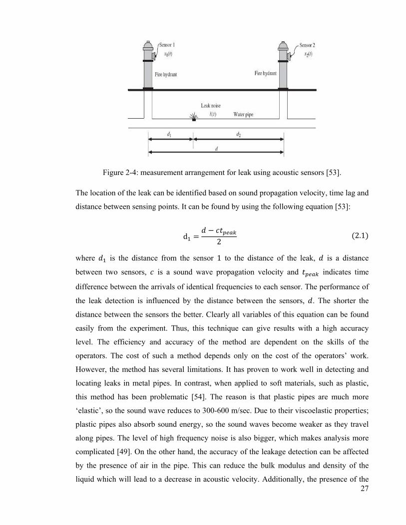
27
Figure 2-4: measurement arrangement for leak using acoustic sensors [53].
The location of the leak can be identified based on sound propagation velocity, time lag and
distance between sensing points. It can be found by using the following equation [53]:
d 2 2.1
where is the distance from the sensor 1 to the distance of the leak, is a distance
between two sensors, is a sound wave propagation velocity and indicates time
difference between the arrivals of identical frequencies to each sensor. The performance of
the leak detection is influenced by the distance between the sensors, . The shorter the
distance between the sensors the better. Clearly all variables of this equation can be found
easily from the experiment. Thus, this technique can give results with a high accuracy
level. The efficiency and accuracy of the method are dependent on the skills of the
operators. The cost of such a method depends only on the cost of the operators’ work.
However, the method has several limitations. It has proven to work well in detecting and
locating leaks in metal pipes. In contrast, when applied to soft materials, such as plastic,
this method has been problematic [54]. The reason is that plastic pipes are much more
‘elastic’, so the sound wave reduces to 300-600 m/sec. Due to their viscoelastic properties;
plastic pipes also absorb sound energy, so the sound waves become weaker as they travel
along pipes. The level of high frequency noise is also bigger, which makes analysis more
complicated [49]. On the other hand, the accuracy of the leakage detection can be affected
by the presence of air in the pipe. This can reduce the bulk modulus and density of the
liquid which will lead to a decrease in acoustic velocity. Additionally, the presence of the

28
suspended solids in the liquid will make liquid more dense and hence decrease the acoustic
velocity [55].
2.2.1.6 Pig based method.
A pipeline inspection gauge or “pig” in the pipeline industry is a tool that acts like a free
moving piston inside the pipe. Generally, in the oil and gas industry the pig has been used
for cleaning, inspection and capture and record the geometric information relating to the
pipelines [56, 57]. Recently, the Water Research Centre in the UK has developed a system
(called Sahara) to detect and locate the leaks in transmission mains. As described by
Chastain-Howley and Mergelas [58, 59] the Sahara system is the only technology currently
available for leak detection and location system that employs a pig based method. Figure 2-
5 illustrated the Sahara system under normal conditions. The Sahara system deploys a
highly accurate acoustic detector unit directly into transmission mains. As a result, leak
detection is taken directly to the leak without being influenced by other factors such as pipe
material, pipe diameter and soil type. The inserted sensor travels along the pipe with the
flow. The sensor is connected by an umbilical cable to a built in tracing device, which
allows the tracking of the position of the sensor accurately from above ground. As it passes
any leak, the sensor head will stop and location of the leak can be identified precisely.
Meanwhile, quantification of the acoustic signal recorded by the sensor can be used by the
operator in order to analyze the magnitude of the leak. It is possible to survey up to 2 km
per insertion. The disadvantage of this system is relatively expensive, both to purchase and
to operate.
Figure 2-5: Schematic representation of Sahara system [58].

29
2.2.2 Leak detection based on internal methods.
The internal method is based on the monitoring of internal pipeline parameters (pressure,
flow and temperature) with the use of instruments to measure internal hydraulic conditions
[42]. Examples of this method are pressure point analysis, mass/volume balance,
hydrostatic testing, negative pressure wave, statistical analysis and frequency analysis.
Generally, the effectiveness of the internal based methods depends on the uncertainties
associated with the system’s characteristics, operating conditions and collected data.
2.2.2.1 Hydrostatic-testing
Hydrostatic (or hydro) testing is a traditional method of determining and locating leaks by
examining each length of pipeline as it is laid. This method previously been used in water,
oil and gas industries to test the integrity of steel pipes [60]. This involves sealing of the
two sections of the pipes and pressurizing the pipes with the water. This method also
requires the measurement of pressure and temperature, over a certain period of time,
usually 24 hours. Any reduction of the pressure show by pressure sensors which is placed
in the pipe could indicate the presence of a leak. This technique fairly good because leaks
can be found when the pipe has just been placed and the leaking pipe can be easily replaced
with a new one. The only problem with this technique is that it cannot easily be conducted
with existing pipeline networks, due to the interference of normal operating where some
section of the networks needed to be shut down. Meanwhile, the temperature measurement
for the buried pipes involves excavation at the pipe sites in order to prevent the ambient
temperature affects the reading of measurement.
2.2.2.2 Mass balance method
Mass balance (and volume balance) are, in effect the same method based on the principle of
conservation of mass [61, 62]. The principle states that a fluid enters the pipe section either
remains in the pipe section or leaves the pipe section. In standard pipeline networks the
flow entering and leaving the pipes can be metered. The mass of fluid can be estimated
from the dimensions of the pipe and by measuring the state of variables such as volumetric
flow rate, temperature and pressure. A leak can be identified if the difference between
upstream and downstream flow measurement changes by more than established tolerance
[63]. This technique allows the detection of the leak that does not necessarily a produce a

30
high rate of change in pressure or flow [43]. This approach is already commercialized and
has been used in the oil pipeline industry. This method also very sensitive to pipeline
instrumentation accuracy. The main weakness of the mass balance method is the
assumption of steady state. As a result of this assumption, the detection period has to be
increased in order to prevent false alarms. Therefore, the response time to the leak will be
delayed, which is undesirable. Another significant disadvantage of mass balance method is
location of the leak is unknown. Consequently, in real application other methods are
required in conjunction with mass balance method after the leak has been detected to
identify the location of the leak [64].
2.2.2.3 Pressure point analysis (PPA)
This method detects the occurrence of leaks through comparing the current pressure signal
against a running statistical trend taken over a period of time along the pipeline by pressure
monitoring and flow monitoring devices [63]. This approach based on the assumption of
the pressure drop if the leak present. Using an appropriate statistical analysis of most recent
pressure measurements, a decrease in the mean value of a pressure measurement is
detected. If the mean of newer data is smaller than the mean of older data, then a leak alarm
is generated. This method may require sensitive high resolution but not necessarily accurate
instrumentation and computer resource requirements and therefore, lower overall
installation costs. Furthermore, this method able to identify the occurrence of leaks, but not
necessarily the presence of them. Since this method use of pressure drop as a leak
signature, it can yield false alarms as the pressure drop is not unique to the leak event even
when the leak signature is correctly identified [64]. .
2.2.2.4 Statistical analysis model
A statistical leak detection system, for example, Atmos pipe has been developed by Shell
[65] that uses advance statistical technique to analyze the flow rate, pressure and
temperature measurements of a pipeline. An optimum sequential analysis technique
(Sequential Probability Ratio Test) is applied to detect changes in the relationship between
flow and pressure, based on relative changes in mean values and pattern recognition of
these discrepancies [66]. This method is appropriate for complex pipe system as it can be
monitored continuously for continual changes in the line and flow/pressure instruments.

31
The main objective of this system is to minimise the rate of false alarm. It is also suitable
for real time application and has been successfully tested in oil pipeline systems [65]. The
main disadvantage of statistical leak detection is that noise interferes in the statistical
analyses, and some leaks were hidden in the noise which prevented them from being
detected.
2.2.2.5 Transient based methods
A leak is a hydraulic phenomenon and has a specific location. It is therefore, clear that its
presence can be detected hydraulically, and that a transient pressure wave is an ideal
vehicle with which to find out where it is. In hydraulic systems, one common method for
wave generation is through the water hammer phenomena [67]. The selection of
measurement and the characteristics of the generated transients depend on the technique
that is used for further analysis.
With any sudden changes in the flow or pressure conditions, for example closing or
opening a valve or stopping a pump, a transient pressure wave is produced, which
propagates along the pipeline. Any change in the physical structure of the pipeline system,
such as a change in section, junction, resistance or leak alters the wave. Generally, the
wave is partly reflected, partially transmitted and some of it may be absorbed at a feature,
thus altering in some way a system’s flow and pressure response (Figure 2-6). Meanwhile,
the speed that the wave travels at depends on characteristics of the pipe and fluid. As a
result, each water distribution system will have different transient behaviour that depends
upon the various devices within the system.

32
Figure 2-6: Pressure time history during transient due to the closure of the start valve (top).
Detail of the initial pressure wave, including the reflected wave from the main (bottom)
[68].
Generally, when a leak occurs the difference of pressure between the outside and the inside
of the pipe causes sudden fluid loss and the pressure of the leak point drops suddenly hence
a rarefaction (negative pressure) wave is produced in the pipeline. Pressures transducers
can be used to measure the pressure with respect to time. Transients propagate back and
forth throughout the network and therefore, can be shown to carry information of leaks or
features within in the pipeline system [69]. Besides its potential low cost and non intrusive
nature, this technique has the potential to locate leaks at greater distances from a
measurement point than is currently possible. Practically, performance of each leak
detection method varies considerably depending on the vendors, pipeline operating
conditions and quality of the hardware/instrumentation system available. It is shown that
there is no method, which is good for all the required attributes. However, when there is
strong noise present in the pressure measurement records or when a leak is too small or too
slow, it can obfuscate the leak reflection signals [70]. A perusal number of hydraulic
transient based techniques for leak detection are described in existing literature: direct
transient [71], inverse transient analysis [[69], [61] ]impulse response analysis [72-74],
transient damping methods [75], frequency domain response analysis [76] and wavelet

33
analysis [77, 78]. The main aim of all transient leak detection methods is the same –to
extract as much as possible the information from the measured transient trace in order
detect and locate the presence of a leak. As mentioned, a leak affects the transient by
increasing its damping rate [75] and creating reflected signals in the resultant trace [68, 79].
Therefore, identification and quantification of these effects is paramount of all transient
leak detection and location technique [70].
One promising early pressure transient technique for leak detection was experimentally
conducted by Silva [71]. The online computational system has been developed based on the
monitoring of pressure for a leak induced pressure wave. Four pressure transducers are
connected to a computer and leak simulated at different locations along the pipeline. The
position of the leak can be found by estimating the arrival time of the negative wave at the
transducers and the knowledge of the wave speed. The method is known as the rarefaction
wave method, involved with the detection of the low‐pressure surge generated by pipe
rupture. It is reported that the leak distance to the sensor and Reynolds numbers are also
significant since the pressure signal decays exponentially with the distance and very rapidly
for low Reynolds numbers, [71]. However, the existence of the background noise made
it difficult to detect accurately a small pressure signal of an unknown shape which will be
the leak. Meanwhile, Jonsson [79] studied the effect of the small leaks on pressure transient
using computer simulations and laboratory experiment for a single pipeline. On his later
study using polyethylene pipes, Jonsson [68] showed that both positive and negative
transients can be employed for leak detection. The analysis of the results identified two
possible leaks.
Covas and Ramos [80] also make use of transient analysis both by identifying the first
wave reflected by the leak and by the free damped pressure, oscillation produced in the
transient regime. They utilized method of characteristics (MOC) [81] in their mathematical
simulation. Their approach focuses on the time analysis of the first reflected wave and the
frequency analysis of pressure variations in order identify the location of leak and
frequency associated with the leak. Both approaches are appropriate for leak location for
single pipelines.
Brunone [82] utilized a transient test for leak detection in outfall pipes. The location of the
leak was determined by timing reflected pressure waves and speed of the sound. In this

34
study, the effect of a leak on wave propagation has been evaluated for both numerical
modeling and laboratory experiments. The signals were detected by comparison of the no
leak transient and the observed trace. The occurrence of transient damping verified the
presence of a leak and the timing of the damping determined the location of a leak.
Brunone and Ferrante [83] conducted experimental measurements based on unsteady
pressure waves initiated by the closure of an upstream valve for detecting and locating
leaks by modeling them as orifices. In their work, a number of orifices discharging into the
atmosphere or submerged were examined. They could predict the location of a leak by
measuring the time for a pressure wave to travel from the leak point to the measurement
section.
Wang [75] proposed a new technique for leak detection in a simple pipeline system based
on the leak induced damping effect on the pressure transient time trace. They observed that
all Fourier components (transient component) were damped uniformly by steady pipe
friction. Based on this observation, the various damping ratios for the Fourier components
are used to pinpoint the location of the leak. The rate of the leak induced depends on the
pressure in the pipe, leak characteristics and location of transient generation point.
Although, their technique is straightforward to employ it is not applicable to complex
pipeline networks due to the waveforms produced by other physical elements within the
network. Furthermore, they also failed to identify which half of the pipeline has the leak
since the damping ratio is similar to two leak locations.
During the wave propagation in the pipeline, the transient is affected by the friction of the
pipe wall and other loss element such as leaks. This effect results in damping of the
transient wave. The leak can be determined via the comparison of the transient damping in
the pipeline with and without a leak. Liou [72] described a method for identifying leak
reflection using determination of the system’s impulse response function. He used a cross-
correlation approach to locate the position of the leak from the first reflection of the
pressure wave from disturbance in the flow profile cause by the leak. The accuracy of the
leak location depends on the discretization of the pipe length.
Although in the forward based analysis, demands and network characteristics are known,
and the objective is to determine pressures and flow rates, in the inverse analysis (or back

35
calculation), pressures and flow rates are known, but there are other unknown parameters
like leaks and friction factors. The idea is to determine these parameters using collected
data. The data are recorded for the leak and compared with the data without the leak. The
study by Ligget and Chen [69] was the first that proposed using inverse transient analysis
(ITA) for leak detection. In a previous study, Pudar and Ligget [84] have theoretically
proposed the inverse method for leak detection under steady state conditions but due to lack
of the number of data points, steady state inverse analysis is unlikely to provide definitive
leak detection results. The ITA method for leak detection proposed by Ligget and Chen
[69] used the least square regression between modeled and measured transient pressure
traces. It has been numerically proven that it has the capability of simultaneous leak
detection and pipe friction calibration. Additionally, leakage detection did not seem to
depend upon accuracy of estimation of friction coefficients since the transient wave is
hardly affected in time by these parameters. Since its introduction, the ITA method was
refined and tested by several subsequent studies [74, 85-87]. For example, Vitkovsky [74]
reported on the use a combinatorial optimization technique with the aim to solve the
inverse leak detection problem. Their method employs genetic algorithms (GA) in
combination with inverse transient analysis, to detect leaks in the water distribution system
using numerical modeling. GA’s are a powerful search tool to find optimal solutions and
use evolutionary based principles. A disadvantage of this method is the slow rate of
convergence for large and complex water distribution systems. In addition to many
computer simulations and numerical case studies reported, some researchers such as Covas
[86] and Tang [88] validate the method using experimental laboratory data. To some
extent, field tests have been conducted [89, 90]. In general, these studies introduced
improved optimization methods, sensor placement and developments in transient modeling.
Additionally, the application of the ITA analysis has become more viable and efficient with
the use of more advanced computer systems and pressure logger. However, as summarized
by Misiunas [3] significant work is still needed in order to validate the method in actual
field conditions and further develop it into a practical and effective leak detection and
location technique.
Meanwhile, there are also the studies that utilize the frequency response method [91-93] to
determine the leak detection. In the frequency domain analysis, both the momentum and
the continuity equation in pipes in the time domain can be solved in the frequency domain
36
by assuming sinusoidal variation of pressure and flow. There are two methods that can be
used in the frequency domain either the impedance method [81] or transfer matrix method
[94].
Mpesha [91] uses the analysis of transient response in the frequency domain. The time
domain data were transformed into the frequency domain by using Fast Fourier transforms.
This method required measurement of pressure and discharge fluctuations only at one
location in the pipeline. By comparing the frequency response graph obtained for the
system with and without a leak, the leak location can be determined. Mpesha stated that the
performance of this technique was strongly influenced by the shape of the transient and the
measurement location.
Covas [41] proposed the standing wave difference method (SWDM) for leak detection in
pipeline networks at a certain range of oscillatory frequencies. Spectral analysis of the
maximum pressure amplitude at the excitation site enables the identification of leak
frequencies had been potential to indicate leak positions. This study was also extended to a
conceptual reservoir-loop-pipe-valve system.
Lee [95] introduced a simplifying practical implementation of frequency domain leak
detection techniques, by using the valve operation to generate a frequency response. They
worked on an induced transient of sufficient input bandwidth in order to produce a
complete frequency response, circumventing the need for a steady-oscillatory signal. It was
observed that each transient signal consists of a limited range of frequencies (bandwidth).
Since only the sharp signal contains a large of frequencies, it should be used for transient-
based detection. Several limitations of frequency domain techniques have to be noted, for
example, the number of observable peaks may be low in a short pipe, making the
pinpointing of the leak difficult.
Other works, for example, Brunone [82] and Brunone and Ferrante [83], utilize the
approach based on the detection and location of leaks by analysing the reflected pressure
wave in the transient signal. While simple to apply, background noise can complicate the
leak reflection signals. As with Brunone [82], Beck [96] exploited the discontinuity in the
pressure signal caused by the leak and used an extension of cross-correlation analysis
techniques to locate the position of a leak. By using the fact that each change in gradient of

37
the cross correlation indicates an event, they could use more of the wave than that which
would just identify the first reflection. Using models and experimental work they showed
that it was possible to find the lengths of all the pipes in a network. They also used the
method to identify leaks in a network, both around bends and also when the leak was
separated from the pressure transducer by junctions. One of the most powerful features of
this type of work was that by analysing the signals and looking for features in the time
domain, no calibration was required.
More recently, studies by Ferrante and Brunone [92] and Ferrante [97] use wavelet analysis
to detect local singularities due to presence of a leak in the measured transient signal. As
suggested by Young [98] the wavelet transform is the best suited for detecting
discontinuities in data traces and is therefore affected by the shape of injected transient.
Ferrante and Brunone [92] make use of a wavelet transform to analyse the experimental
pressure history, generated in a simple pipeline, caused by sudden valve closure with leak
and without leak. It is reported that by using suitable wavelet bases the occurrence of the
leak induces local discontinuities in the pressure signal can be detected and captured. They
utilized Daubechies wavelets for the transform and used the holder exponent to determine
the singularities corresponding to the leaks. Meanwhile, Stoianov [99] applied the concept
of artificial neural networks to analyze the feature vectors of the wavelet coefficients
attained by wavelet decomposition for locating and quantifying leaks. In their latest study,
Brunone [100] demonstrated transient tests generated by the portable pressure wave maker
(PPWM) occurring in pressurized pipe systems. It produced small amplitude sharp pressure
waves that allow locating and evaluating the feature of the network such as leaks, partial
blockages and negligently partially closed in-line valves. Wavelet analysis is being used to
improve the precision of the pinpoint of anomalies. As the result, it was proven that the
transient test-based techniques can be used for both localization and evaluation of the
features of the pipeline network.
Al-Shidhani [77] also performed wavelet transforms on experimental and simulated
transients in pipe systems. The technique identified singularities in the simulated data;
however, when the same analysis was applied to the experimental data, the expected results
did not agree with the lengths found in the network. This is because the waves spread out
due to dispersion [101] causing the outgoing and incident waves have different

38
characteristic frequencies. To overcome this problem, Beck [102] used the cepstrum [103]
function to analyse their pressure histories and identify leak positions in pipeline networks.
This function has the ability to identify families of frequency harmonics associated with
pressure wave reflections form the leak. The method not only detects the leaks but is also
able to estimate their severity. More recently, the studies by Taghvaie [104, 105] using
orthogonal wavelet transforms in conjunction with cepstrum confirm that this method can
detect leakage size and location in pipelines. Wavelet de-noising was used for pre-
processing of the signal before application of the cepstrum. Their method has been
successfully implemented for laboratory experiments and field tests.
2.3 Summary
In this chapter, many different methods for leak detection and location in pipelines
networks have been described. These methods are divided into two main categories:
external method and internal method. The external method approached detects the leaks
from outside of the pipe using specific devices, in which some cases the cost is very high.
Alternatively, there is the internal method, which deals with the measuring of hydraulic
change in the pipeline. The internal approach is most popular among the researchers due to
the cost effective of this method. Additionally, the internal method tends to be divided
further into two fundamental approaches: that of analysing the response systems to
ascertain their condition, and reverse engineering the results from the response of a
network. This latter method involves using a model of the physics and optimising the
parameters of a model to fit experimental transient data. While the using former method,
the features in the system can be determined by signal analysis of the reflected pressure
wave in the transient signal.

39
Chapter 3
Propagation of Waves in Pipelines
3.1 Introduction
In general, a wave can be described as a disturbance that propagates through a medium
from one point to other points as a result of energy and momentum change through a small
displacement of the molecules of the medium between these two points. This disturbance is
transferred from one molecule to the next molecule and causes a wave in the medium.
Consequently, the density of the fluid is changed instantaneously, which then produce
waves that propagates through the system [24]. Examples of this in the operation of water
distribution systems include: opening or closing a valve or the starting and stopping of
pumps. The faster these operations are performed too, the greater the magnitude of the
hydraulic transient that will occur. In general, transients resulting from the rapid changes in
flow rate are referred to as water hammer phenomena. As a result, a transient pressure
wave is produced, which propagates along the pipeline. If the magnitude of this transient
pressure is excessively high, and suitable control measures have not been installed in the
system, it can cause a number of adverse effects on the pipe system [24]. In order
understand the water hammer phenomenon in a hydraulic system, the concept of
propagation of a liquid within a pipeline is necessary.
3.2 Water hammer phenomenon in a pipeline
Water hammer refers to the transient conditions in a hydraulic system that prevails
following the sudden change of flow in a pipe. More generally, it is a pressure wave which
results when a fluid in motion is forced to stop or change and there is a momentum change
in it. Let us first examine some of the common things that accompany the phenomenon,
and later explore more on the associated attributes. Consider a simple hydraulic system
consisting of two reservoirs with a valve positioned at the mid-length point of a straight
pipe carrying fluid between two reservoirs. The two pipe sections upstream and
downstream of the valve are identical in all respects. When a valve is suddenly closed, it

40
causes the nearest fluid to the valve to be compressed, and then brought to rest. Due to the
pipe walls, this compression cannot cause a change in volume, and hence the pressure rises.
This increase in pressure at the valve results in the wave being propagated upstream,
bringing the fluid to rest as it passes, compressing it. As a result, the compressed liquid will
now start to release liquid in the pipe back to the source and return to the static pressure of
the source. As the wave arrives at the upstream end of the pipe, the mass of fluid will be at
rest but under great pressure. This creates an unbalanced condition at the upstream
(reservoir) end at the instant the pressure waves arrive, since the reservoir pressure
unchanged and all kinetic energy has been converted into elastic energy [67, 101]. This
process of conservation travels downstream towards the valve at the speed of sound in the
pipe, which depends on the properties of the fluid and the pipe material. Similarly, on the
downstream side of the valve, the retardation of flow results in a reduction in pressure at
the valve, with the result that a negative pressure wave is propagated along the downstream
pipe, in turn, retards the fluid flow. The sequence of events after sudden valve closure in a
frictionless system is shown as Figure 3-1.

41
Figure 3-1: Valve closure in a frictionless system [24].
The well known Joukowsky [67] equation has been applied for sudden closures in
frictionless pipes and given as:
3.1

42
where the rate of change in pressure ( Pa/s), is fluid density (kg/m3), is the
characteristic wave velocity of the fluid (m/s), is the rate of change in fluid velocity
(m/s2). An alternative and useful form to express the pressure change in terms of a change
in pressure head, by dividing both side of Equation (3.1) by to gives:
Δ Δ 3.2
The equation shows that opening a valve causes a positive velocity change followed by a
reduced in pressure. Conversely, if the valve closes (producing a negative ∆ ), the pressure
change will be positive. A similar set of equation may be developed for a wave propagating
in the downstream direction and given as:
Δ Δ or Δ Δ 3.3
The wave propagation speed a will be dependent on the pipe diameter and material,
theoretical values for which can be found in several text books. It represents the
compressibility of the fluid and the distensibility of the pipe wall. Thorley [67] gives the
speed of wave propagation in the thin walled pipes (where internal diameter, D is greater
than 10 times of wall thickness, e) as:
11 3.4
where wave propagation speed (m/s), fluid density (kg/m3),
Young’s
modulus of elasticity for pipe wall material (N/m2), bulk modulus of the liquid
(N/m2), and a restraint factor dependent on the Poisson’s ratio of the wall material
and how well the pipe is supported. Equation (3.4) is only true for single phase fluids in
rigid pipes whereas for the flexible pipe or the fluid is multiphase, the speed of wave will
be decreased [106].

43
3.3 Ideal propagation of transient pressure waves in pipe
When a pressure surge travel along a pipe, at every discontinuity of the system such as a
leak, bend, valve, junction or change in pipe diameter, the wave is partially reflected back,
partially transmitted forward and some of it will also be absorbed [18]. Neglecting energy
losses along the pipeline, and at the singularity, the reflected wave added to transmitted
wave equals to the incident wave as shown in Figure 3-2.
Figure 3-2: Conceptual wave reflections at a leak [107].
A leak induces a sudden pressure drop in a positive pressure surge, and also a reflection
point. In a transient wave in a pipeline, the signal and leak-reflected signals could take
multiple paths due to boundary reflections. A transient event in a pipeline is represented in
Figure 3-3.
Figure 3-3: Transient propagation in pipeline systems [70].

44
As we can see from the figure, two different paths that the signal could have traveled to
generate a leak reflected signal labeled as (a) and (b) while the original transmitted signal
continues to move downstream [70]. Note that the time arrival of the reflected signal can be
associated with either one of these paths. Furthermore, in comparison with the blockage, a
leak is a flow loss element without head lost, and a blockage is a head loss without flow
loss. As a result, when a wave encounters a leak, it causes a pressure relief to the impulse
and reflected portion of the wave is the opposite sign to the initial wave. Also when, a
pressure wave interact with a blockage, the reflected wave returns with the same sign as the
initial wave [108].
3.4 Effect of a leak on a pressure wave A pipeline running between two boundaries is considered here as an example. In some
cases, the transient generating and measuring device might have to be installed separately,
or close to each other but somewhere in the middle of the pipelines as shown in Figure 3-3.
As suggested, the leak detection procedure should not interrupt the operation of the
pipeline. The generated transient response and the pressure measurement point are located
at point G and M respectively.
Figure 3-4: Pipeline with a leaking point and two boundaries [109].
As the transient generation point is located along the pipeline, two waves will be generated
(upstream positive and downstream negative) which will propagate in opposite directions
towards boundary 1 and 2. Consequently, as shown in Figure 3-4 the leak, L is simulated at
a distance Xleak from the generation point in the direction of boundary 2.
The procedure of transient wave propagation and its reflection in pipelines is summarized
in sequential steps as displayed in Figure 3-5. It is assumed that the transient generation, G

45
and pressure measurement, to be located at the same point which is same as the
experiment works in this research. The generation and measurement points should be
located as close to each other as possible. If the leak occurs in between the measurement
and generation points, the location of it becomes more complicated. The generated transient
wave is reflected from the leak before it reaches the measurement point. As a result, the
reflection of a generated wave from the leak is no longer detected in the measured trace.
The pipeline system from Figure 3-4 is considered where the leak to be positioned at .
At the transient start time, two transient waves which are 1 and 2 generated at point
G and propagate in both directions along the pipe (Figure 3-5). At time / as
the 2 arrives at the leak, part is reflected backward and another part is transmitted
towards boundary 2. The leak reflected wave, 1 has the magnitude equal to Δ . At the
instant 2 after the closure, the reflection 1 arrives at the measurement point.
At this time, the difference between the pressures for no-leak and leak case, i.e.
, becomes equal to (neglecting frictional effects). Meanwhile, at the time
, / the wave 2 have reached boundary 2, 2 and reflected from it where the
magnitude of reflection depends on the reflection coefficient of the pipeline boundary, .
The reflected wave from 2 reaches the leak point at time , / and
again part of it is reflected 2 . The magnitude of reflected 2 slightly smaller than .
At time 2 , , the remaining part of 2 arrives at measurement point. The wave
1 reaches the measurement point at time 2 , (after it was reflected from the
boundary 1, 1) with the same magnitude as for the no leak case since there is no leak
exists between the measurement point and 1
In this example, a singularity in the transient traces is generated by the arrival of the leak-
reflected signal at the measurement point. The location of this singularity in the trace
designate the arrival time of the leak-reflected signals. This indicates the time needed for
the transient signal to travel from its generation point, reflect off the leak and return to the
measurement point. In addition, the amplitude of the reflected wave depends on the leak
size. By increasing the leak size the magnitude of the reflected wave increases and the
amplitude of the incident wave after the leak point decreases [110].

46
Figure 3-5: Transient wave propagation and its reflections from leak and pipelines
boundaries [109].
3.5 Effect of features on the pressure wave
In addition to the effect of the leak on a transient signal, it is essential to know about
boundaries such as dead ends, pipe junction and tanks which control the behaviour of the
transient event. Generally, the hydraulic systems consist of numerous pipe sections with
differing characteristics such as material and diameter. These segments are joined with
each other's with junctions (or nodes). When a wave encounters a boundary such as a
junction, part of the wave is reflected from the boundary, and another part of the wave is
transmitted across the boundary. On the other hand, the behaviour of reflection and

47
transmission of the pressure wave depends on the material properties on both sides of the
boundary [111]. The transmission of waves through the junction not only depends on the
cross sectional area in all pipes connected to the junction but also the speed of pressure
wave [101].
Consider a node four pipes connected to it as an example to study the effect of a junction
on a pressure wave in a pipeline (Figure 3-6) [24]. A pressure wave, defined by magnitude
Δ travelling in a pipe reaches to a node, it is transmitted to all other connected pipes
with a head value, Δ and also reflected in the initial pipe with the head value, Δ . As a
result, the reflected wave causes a change in the flow and head conditions at each of the
pipes connected to the node. Figure 3-6(a) shows the node as the transient pressure wave
approaches the junction while Figure 3-6(b) shows the node after wave reflection and
transmission. The dimensionless transmission (s) factor can be defined as [24]:
sΔHΔH
2Aa
∑ Aa
3.5
where Δ is head of transmitted wave (m), Δ head pulse (m), is incoming pipe area ( ),
is incoming wave speed (m/s), is area of th pipe ( ), is wave speed of i-th pipe (m/s),
n is number of outgoing pipes, and is pipe number. On the other hand, the dimensionless reflection
(r) factor given as:
rΔHRΔH s 1 3.6
where Δ is head of reflected wave (m).

48
Figure 3-6: Reflection and transmission of wave at junction [24].
Moreover, these two factors can be utilized to verify how waves are transmitted and
reflected at each boundary and branch. As far as the hydraulic system is concerned, the
boundary conditions in a pipeline network are different. For instance, we may have the
scenario where the end of pipe is connected to the reservoir which in turn is connected to

49
either a dead end or a closed valve as shown in Figure 3-7 and 3-8 respectively. Thus, the
reflected wave from these two boundaries is different from each other.
Figure 3-7: Incident wave at reservoir [24].
Figure 3-8: Incident wave at dead-end/ closed valve [24].
In the case of a pipe connected to the reservoir, when the geometry of the outgoing pipe,
1 and the reservoir area ∞ are substituted into Equation (3.5), it is found that the
transmission factor, 0 and the reflection factor, 1. As a result,∆ ∆
meaning that when a wave reaches the reservoir, it is reflected with same amplitude but
with the opposite sign. Also, ∆ ∆ , for this particular case
where as depicted in Figure 3-6 represents final head – head after the wave
reflection/transmission.
Meanwhile, when a pipe is connected to a dead end or a closed valve, 1, and through
the derivation of the Equation (3.5), it can be shown that the reflection factor, 1.
Therefore, in this case, the reflected wave at a closed end of pipe has the same sign; hence
head amplification occurs at that extremity. The reflected wave is twice the pressure head
compared to incident wave. It is the same amplitude. If a flow control operation creates a
negative pressure wave that arrives at a closed end, the wave’s reflection causes a further

50
reduction in pressure. As a result, this transient flow condition can cause a potential
pipeline collapse in low head systems. It is also possible to have a pipe diameter increase in
the pipeline system as displayed in Figure 3-9.
Figure 3-9: Incident wave at diameter increase in pipe [24].
In this case, an attenuation of the incident head occurs at the pipe diameter increase. The
smaller pressure wave is transmitted to larger pipe as the change in volume is spread out
over a larger area. As a consequence, after the reflection, the smaller pipe experiences a
lower final head. At an expansion, only part of the wave subjected to reflection.
Some pipes have an open end shape, and at the point when the pressure wave arrives at the
open end, it is reflected by the boundary condition of the open end and propagates back
along the pipe, with an inverse phase to the incident pressure wave as shown in Figure 3-
10.
Figure 3-10: Pressure waves in an open-ended pipe [112].
Some parts of the pressure wave, which reaches the open end of the pipe, is discharged
from the open end. As a consequence of momentum of pressure wave, the fluid leaves the
pipe into the open air, i.e., atmosphere, which sequentially might cause the fluid to be

51
scattered in different directions. Because of the spread out of flow in different directions, its
pressure drops to the pressure in outside of the pipe (often atmospheric pressure).
3.6 Dispersion and attenuation
When a pressure wave propagates through a fluid filled pipe, two characteristic processes
take place. Firstly, the front of the wave becomes spread out (dispersion) and, secondly, its
amplitude decreases (dissipation or attenuation). The phenomenon of dispersion can be
described as Figure 3-11(a) and 3-11(b). As illustrated by black wave pulse, which is a
Gaussian function, containing multiple frequencies. If the wave speed depends only on the
physical properties of the medium, then the wave speed is a constant, independent of
frequency. Such a medium is called a non-dispersive medium and waves traveling through
this medium will maintain a constant shape. Since the wave speed is constant, all
frequencies travel at the same speed and the pulse maintains constant shape as shown in
Figure 3-11(a) and 3-11(b).
On the other hand, there are many examples of dispersive media where the wave speed
depends on the frequency of the wave. As illustrated by the blue wave pulse in the Figure
3-11 is the same Gaussian function as the black pulse, consisting of a large number of
frequency components added together. However, now the wave speed depends on
frequency, with higher frequencies traveling faster than lower frequencies. As a result, the
wave pulse spreads out and changes shape as it travels as shown in Figure 3-11(a) and 3-11
(b) [113].
Figure 3-11: Dispersion of wave pulse [113].
a) b)

52
Additionally, the effective fluid inertia associated with a depth of penetration of
disturbances depending upon the wavelength, causes dispersion: a dependence of wave
speed upon the wavelength. The transient wave form is also modified by the phenomenon
of dispersion. In frictional flow, highest frequencies travel at a higher (near isentropic)
wave speed than low frequencies. Because of the rapid decay of the high frequency
components, dispersion effects diminish as transient propagate [101]. It is well known that
when waves are transmitted through a waveguide such a pipe, the signal suffers dispersion;
that is, the component frequencies in the signal travel at different speed and as a result the
signal spreads out and less sharp. Thus, the information is altered in its path from the
source to the receiver (pressure transducer).
In a system without friction or tanks to dampen transients, transients could conceivably
persist indefinitely. However, viscous and friction effects and loss of momentum in tanks
typically cause transients to attenuate within seconds to minutes. In a practical pipeline
system, the occurrence of transient state of the flow from an original steady state flow and
changes to another steady state due to the energy dissipation. Some of the incident wave
energy is degraded into heat since of the wave propagation process is not isentropic.
Therefore, wave attenuation is caused by the energy loss from the incident wave in a
medium which fails to respond perfectly to any sudden pressure change [106]. As the wave
frequency increases, the flow changes caused by the pressure pulse propagation become
sharper and more numerous per unit time, resulting in more energy absorption. The
molecular interactions between neighbouring flow layers (laminar flow) and flow eddies
(turbulence) resist the wave passage and lead to energy loss.
For illustration, the pressure head signal for a practical pipeline in a typical water hammer
event is attenuated and reflected with time in the manner shown in Figure 3-12 [114].

53
Figure 3-12: (a) Top left- Elastic pipeline for a water transportation system (b) Top right-
Transient pressure head trace in the elastic pipeline (Adapted from Stephens [115]) (c)
Middle left- Visco-elastic pipeline for an urban drainage system (d) Middle right- Transient
pressure head trace in the visco-elastic pipeline (Adapted from Covas [41] ) (e) Bottom
left- Randomly varying pipe diameters due to corrosion (f) Bottom right- Transient
pressure head trace in the disordered-diameter pipeline (Adapted from Duan [114]).
In the previous study, the Sheffield [77, 102, 110] group has proposed few methods to
overcome the problem with dispersion. In the current research, another analysis technique
was utilized in order to obtain the important information buried in the collected data.

54
3.7 Effect of noise in the system
In a pipeline system, one of the main challenges to the researchers is the issue of noise,
contributed from many resources. All of which cause difficulties in the separation of the
leak signal from a vast range of other disturbances and events. In this research in order to
circulate the flow in the pipeline system, a pump is used. However, pumps are often noisy
because they are sitting directly on a base with no anti-vibration insulation between them
and also due to the piston or blades it produces some noise in a raw data. And also for the
generation of a pressure wave in a pipeline it is necessary to apply a solenoid valve which
by periodically closing and opening to generate this wave. Since this solenoid valve causes
a water hammer pulses to enter the main network via a short pipe connected to a hydrant
valve it can also cause noise in the system. Meanwhile, vibration in length of pipe that is
connected to a pump can result in spurious signals being caused in the pressure transducer
which is attached to the pipeline.
In real systems, the presence of small air bubbles can be spread along the pipeline, which
cannot be thoroughly removed, and these can create the artificial noise in the transient
pressure signal. Additionally, there was also noise created by reflections of different pipe
materials and diameters, particularly in cast iron pipes [116]. All these noises can
considerably affect the success of any leak location technique as their amplitude can be
close to the size of the waves reflected from leaks during transient events. In order to
remove noise from raw data filtering must be used.
3.8 Summary
This chapter presents the basic concepts associated with the propagation of transient
pressure wave in the pipelines due to any change in the flow or pressure in a fluid in a pipe.
When this wave has been induced in the pipeline system, it will encounter any features or
boundary such as leaks, changes of pipe diameter, blockage and tee junction. As a result,
when a wave reaches any feature, some of it is reflected back and of it is transmitted along
the pipe. The detection of these signals allows their identification and location.

55
Chapter 4
Signal Analysis Methods for Leak
Detection
4.1 Introduction
Successful leaks or blockage detection becomes a vital activity that involves more than
just economic convenience, with issues of resource conservation and environmental
wellbeing [29]. Studies by a variety of researchers show that transient tests using water
hammer create a pressure wave that ultimately propagates throughout the entire pipeline
network. Portions of this are reflected back from various pipeline features. Irregularities in
a pipe system provoke discontinuities in this pressure signals so that the problem of leak
and features detection is akin to the investigation of signal discontinuities as the pressure
wave is constituted of such irregularities. The using of advanced signal processing
techniques should make it possible to identify and locate of these discontinuities through
the analysis of the corresponding pressure time response signal; obtained through a single
sensing device [76].
Essential information corresponding to abrupt transitions in pipeline system traits is
embedded in the signal. Traditionally, Fourier analysis has been used to analyze the
response data of systems [117]. Without knowing when a leak has occurred, inaccurate
results have been produced due to its time integration over the whole time span. This is
because simple signal analysis techniques assume that the wave does not change much in
characteristic frequency. Since the signal produced during the transient process is mostly
non linear and non stationary, new method of analysis is required. The most successful of
these used to date is the to cepstrum analysis technique [118]. The mathematics behind this
will be described later.
Generally, cepstrum can detect the periodic structures in the spectrum and identify the
presence of the echo. However, the performance of cepstrum will be affected by the
presence of noise in the signal. As a result, filtering of the signal is required to remove

56
unwanted features, e.g. noise, trends or frequency component. Many methods of filtering
could be used to remove noise. Recently, a new type of time-frequency analysis called the
Hilbert-Huang transform (HHT) has become more popular for analysing non-linear and
non-stationary signals. The HHT is totally adaptive and has been developed by Huang
[119]. This method consists of empirical mode decomposition (EMD) to produce intrinsic
mode function (IMF), followed by a Hilbert transform (HT) analysis. HHT techniques have
been applied to various fields, such as structural damage detection [120], , bioscience [120]
, and filtering and denoising [121] . In order to understand the detail of mechanisms for
non linear and non stationary responses, processed calculation of instantaneous frequency
(IF) is necessary. Historically, HT has been used to calculate the instantaneous frequency.
In the recent study, different approach has been implemented in order to compute IF such
as Normalize Hilbert transform (NHT), Direct Quadrature (DQ), and Teager Energy
Operator (TEO).
In the following sections, detailed formulations of Fourier transform and the time-
dependent (short-time) Fourier transform are presented. Followed by, the discussion of
cepstrum analysis. A brief discussion of the continuous wavelet transform (CWT) and
discrete wavelet transform (DWT) also presented. Then, the empirical mode
decomposition, Hilbert Huang transform and instantaneous frequency are presented in
detail along with appropriate examples.
4.2 Fundamental Concepts
4.2.1 Fourier Transform
For the sake of completeness the traditional frequency analysis, Fourier transform (FT) is
briefly described in the first part of this chapter. Generally, time domain signals do not
provide good information about frequency content and are not always the best
representation of the signal for many signal processing related applications. Often the vital
information is buried in the frequency so that the signal has to be converted from the time
domain to the frequency domain. The Fourier transformation as a mathematical linear
transformation has been used in different fields [121]. In essence, the Fourier transform of
any periodic of non-periodic or signal of limited duration could be decomposed or
separated from some set of sinusoids, terms of different frequency, amplitude and phase.

57
The Fourier transform is then a frequency domain representation of a function.
Mathematically, in the case of a continuous time-signal of this process which is
represented by:
4.1
Meanwhile, the original function can be recovered from its spectral with the inverse Fourier
transform given by:
4.2
In above relations, 1− , is the continuous function in time and is its
corresponding Fourier transform, which is a continuous function in frequency. As it can be
seen in the above equation, integration is carried out over the entire signal and the
frequency components of signal are extracted. However, Fourier analysis provides only
frequency information and the time data associated with those frequencies is lost with no
time information remaining in the transformed signal. When analyzing stationary signals
whose statistical properties do not vary with time, the time information is not always
crucial, particularly where the frequency contents of the signal do not change over time: in
other words, all frequency components must exist at all times. In contrast, where the time
data in non stationary signal whose statistical properties change with time is crucial
transforming them using the Fourier transform causes time information loss. Consequently,
it is not possible to recognize at what time each frequency component occurred.
Furthermore, non stationary signals are divided into continuous and transient types. In real
engineering applications, we often deal with the signal which is mostly non stationary
[122]. .
In order to incorporate both time and frequency localization properties in one single
transform function, the Short Time Fourier Transform (STFT) was developed. This
approach provides a time-frequency representation, commonly referred to as spectrogram
[122] . The basic idea behind STFT approach is that a non stationary signal is divided into
small segments or portions, such that each segment of the signal can be assumed to be a
stationary signal. To divide the signal, a window function with a suitable width and

58
location is multiplied by the signal and the desired part of the signal is extracted. Each
extracted part can be viewed as stationary so that Fourier transform can be used. In the next
step, the window is shifted to a new location and is multiplied by the signal to extract the
next stationary segment. Then a FT is applied on this product. This procedure continues
until the end of the signal [123] and can be represented as Figure 4-1. The STFT can be
expressed as:
, 4.3
where is the signal to be transformed, is the windowing function, , is the
Fourier transform of multiplied by and represents the amplitude and phase of
over the time and frequency range.
Figure 4-1: Procedure of computing the STFT [124].
Despite the ability to decompose the signal in both time frequency domains, the STFT
suffers from a major drawback where it does not allow a high degree of resolution in both
time and frequency domains simultaneously. This is due to a form of the Heisenberg
uncertainty principle [125] that bounds their products as:
Δ Δ14 4.4

59
The general meaning of Equation (4.4) is that there is a tradeoff between time resolution
and frequency resolution. The STFT provides constant Δ . Δ resolution since the same
window is used for the entire analysis. The performance of STFT is highly dependent on
the window size. Polikar [126] mentioned that frequency resolution was improved if a wide
window is employed, but then the time information becomes poor. On the contrary, if a
narrow window is implemented, it improves the time resolution and it causes a poor
resolution in frequency. Sequentially, it is crucial in analyzing many signals to change the
window size to get a better resolution for both time and frequency. For the purposes of the
work on looking into reflections for leak detection, both temporal and spatial resolutions
are important.
4.2.2 Cepstrum
In recent years, cepstrum has emerged as a powerful new spectral analysis method.
Generally, cepstrum analysis can be useful in interpreting the spectrum, as a tool for
detection of periodic structure. The cepstrum is a non linear signal processing technique
which the original definition introduces the cepstrum as the Fourier transform of the
logarithm of Fourier transform [127].
| | 4.5
where is the power spectrum defined as the Fourier transform of the autocorrelation
function. Cepstrum can be considered as a “spectrum of a logarithmic spectrum” that has
properties which make it useful in many types of signal analysis. The cepstrum can be
found either in power (real) cepstrum or the complex cepstrum. The power cepstrum is a
real valued function and it is the inverse Fourier transform of logarithm of power spectrum
of a signal. It can be used for the identification of any periodic structure in a power
spectrum such as the detection of turbine blade or gearbox faults [128]. Meanwhile, the
complex cepstrum is defined as the inverse Fourier transform of the logarithm of the
forward Fourier transform of a time signal.
4.6
where is the complex spectrum of and can be represented in terms of the
amplitude and phase at each frequency by:

60
4.7
Taking the complex logarithm of Equation (4.7) gives:
| | 4.8
where, √ 1 and is the phase function.
Cepstrum can help to identify items, which are not readily found by spectral
analysis as it has the ability to identify periodic structures in the spectrum, such as families
of harmonics and/or sidebands with uniform spacing. Another of the cepstrum’s effects is
that it is capable of identifying the presence of the echoes. The power of this technique
even extends to reflections that are not perfect copies of the original signal. It is thus ideal
for extracting information on the time delay between the creations of a wave and receiving
the reflection of that signal. Since the complex cepstrum holds the information about the
amplitude and phase of the spectrum so it is reversible back to the time signal, it is a good
tool for signal separation, bringing to the signal the effect of deconvolution, as explained in
Randall [127]. Let consider a simple example how cepstrum work, a 20Hz sine wave
sampled at 100Hz as:
sin 2 20 4.9
Now consider an echo of signal with half amplitude and 0.4 seconds after the beginning of
the signal is added to original signal and plotted as Figure 4-2.
Figure 4-2: Example signal with an echo

61
The complex cepstrum of this new signal is shown in Figure 4-3 below:
Figure 4-3: The complex cepstrum of the signal with an echo.
It is found that the complex cepstrum is able to detect and measure the reflection delays in
the signal. The effect of this reflection is seen clearly in the cepstrum at 0.4s as a peak
which is not all evident in the time domain signal.
4.2.3 Wavelet
Wavelet analysis effectively began in 1990s and was seen to offer an alternative to
traditional Fourier bases for representing functions [126]. Wavelet is recognized as a
powerful tool for signal processing analysis due to its ability to analyze signals containing
discontinuity or sharp changes as well as noisy or transient waveforms. Wavelet is widely
used as an efficient tool for speech recognition [129], medical signal monitoring [130],
image processing [131] and condition monitoring of machinery [132].
The terminology “wavelet” was first introduced, in the context of mathematical transform
in 1984 by Grossmann and Morlet [133]. The term “wavelet” means a small wave with
finite energy, which has its energy concentrated in time or space to serve as a base function
for the analysis of transient, nonstationary or time varying phenomena. The wavelet has the

62
oscillating wavelike characteristics and ability to allow simultaneous time and frequency
analysis. Wavelet has been developed from Fourier transform (FT) [134] with both
techniques analyzing the signal in a similar way as complex numbers (sine and cosine
functions). Wavelet analysis decomposes a signal into set of basis functions, which are
obtained by shifted and scaled versions of a function called the “mother wavelet” [135].
This function is localized in time or space. Thus, the wavelet analysis offers immediate
accesses to information that can be obscured by other time frequency methods such as
Fourier transform. Wavelet analysis may be broadly classified as continuous wavelet
transform (CWT) and discrete wavelet transform (DWT).
4.2.3.1 Continuous Wavelet Transform (CWT)
Continuous wavelet transform is similar to the STFT described above whereby in
both the signal is multiplied by a window function and the spectrum for each portion of the
signal is computed. However, the main difference between wavelet transform and STFT is
that the window width in the WT is not constant through the transform and, indeed, it
changes for each segment of the signal being transformed. The continuous wavelet
transform gives time-frequency decomposition by taking translation and dilations of a (real
or complex) wavelet:
,1√
4.10
where is the signal being transformed, , are called the wavelet coefficients, that
are functions of scale and time location, is a scale parameter which controls the width of
the wavelet; i.e. the local resolution of the wavelet transform in time and frequency domain
and is analogous to [1/frequency], b represents the translation parameter of the wavelet that
governs the movement of the wavelet along the time axis and is the mother wavelet
function. The asterisk in Equation (4.10) indicates that the complex conjugate of is
used in the transform and is applicable when complex analysis is used. Consistent with the
CWT equation, the signal is multiplied by a wavelet and then integrated over time;
mathematically, this operation is called convolution. Furthermore, as reported by
Daubechies [135] the different types wavelets available such as Mexican hat, Gaussian
wave, Haar and Morlet.

63
In contrast to STFT, which has fixed resolution at all times and frequencies, the
wavelet transform provides a multi resolution approach for signal analysis. In general, the
time resolution becomes good at high frequency or low scale, while the frequency
resolution becomes good at low frequencies[126].
4.2.3.2 Discrete Wavelet Transform (DWT)
As mentioned before, in the CWT, scale and shift factors vary continuously over the full
time frequency domains of the analyzed signal. Therefore, this makes the CWT highly
redundant and its implementation may consume significant amounts of time and resources
[126]. In order to overcome this deficiency and to speed up the wavelet transform the
Discrete Wavelet Transform (DWT) has been introduced. The key difference in a discrete
wavelet analysis is that the scale parameter (a) and translation parameter (b) in Equation
(4.10) are no longer continuous, but instead are integers. It is called the Discrete Wavelet
because the wavelet functions used in DWT can only be scaled and translated in discrete
steps. The parameters a and b can be sampled by employing a power of two logarithmic
discretization in which the scale parameter a is discretized on a logarithmic basis and the
translation parameter b is then linked to the scale parameter. As a result, a and b are
rewritten as:
2 , 2 4.11
This power of two logarithmic scales is the simplest and most efficient discretization
method for practical applications and it is known as sampling on a Dyadic Grid. Finally,
the discrete wavelet transform of a continuous time signal is obtained as:
,1
√22
4.12
Related to multi resolution analysis, the DWT acts like a dyadic filter and the signal can be
decomposed into a tree structure with wavelet detail and wavelet approximation at various
levels. The decomposition process is iterated with successive approximation components
being decomposed in turn, while the details are saved each time. Generally, an

64
approximation of itself , at arbitrary scale index and a summation of wavelet
detail coefficients from scale index down to ∞ are as follows:
4.13
4.2.4 Hilbert transform and analytical signal
As the Fourier transform takes a time-domain signal x(t), and moves it into the frequency
domain, the Hilbert transform of x(t) produces another time-domain signal. According to
Randall [127], the Hilbert transform (HT) is a relationship between real and imaginary
components of the Fourier transform (FT) of one sided signal. For an arbitrary signal, x(t),
its Hilbert transform H[x(t)] can be determined by:
4.14
in which PV denotes the Cauchy principal value of the integral. In fact, is the
convolution of with 1/ ; therefore emphasizes the local properties of x(t), even
though the transform is global. Physically, the Hilbert transform can also be interpreted as a
natural /2 phase shifter with changing the phase of all frequency components by /2, as
the magnitude of the signal does not change. As a simple example, the HT of a cosine wave
is a sine wave (or vice versa) of the same frequency and amplitude. This quality of the HT
gives the advantage in using it for data analysis instead of the traditional approach using the
FT. Coupling the and we can have a complex conjugate pair to give an analytic
complex signal of as:
4.15
where a(t) is the instantaneous amplitude equal to:
4.16
and is a phase function of the :

65
4.17
Finally, Equation (4.15) can be written as:
4.18
If we have a signal, ), then we can calculate the signal’s Hilbert transform, and
hence obtain the signal’s phase by combining with . Figure 4-4 shows a simple
sine wave and its Hilbert transform (cosine wave).
Figure 4-4: A sine wave and its Hilbert transform.
Clearly, a phase shift of /2. Furthermore, by using the HT the instantaneous properties of
the analytical signals can be found easily. Since the signal only involves a single frequency
wave, it is found that as shown in Figure 4-5, the instantaneous amplitude of the signal has
the constant value of 1 and the phase function is a straight line that intercepts at -π/2 of the
y-axis.

66
(a) Instantaneous amplitude (b) Instantaneous phase
Figure 4-5: Instantaneous characteristics of the Hilbert transform of sine wave.
However, it should be noted that to obtain meaningful and well-behaved instantaneous
characteristics of the analyzed signal must involve only one mode of oscillation, so called
monocomponent [119]. This type of wave is not common in real engineering problems.
Therefore, it could lead to obtain physically meaningless results.
4.2.5 Hilbert-Huang Transform
As discussed in the previous section, the major drawback of the Fourier transform is
the lack of time localization of the frequency components. Accordingly, there are some
crucial restrictions to Fourier spectral analysis: the system should be linear; and the signal
should be strictly periodic or stationary; otherwise the resulting spectrum will produce little
of physical sense. So far, the wavelet transform may have been the best available signal
processing method for non stationary signals. However, the choice of mother wavelet
function can leave a lot to be desired. Once the function has been selected, it is kept
constant during the analysis and this makes it non adaptive. Consequently, the WT also
only captures those signal features which correlate well with the shape of the wavelet
function; meanwhile, it can mask or ignore the other features [136]. Moreover, the Morlet
wavelet, for example, which is based on the FT, suffers many drawbacks similar to those
suffered by FT. In the WT the time and frequency resolution is a compromise whereby the
WT is unable to achieve fine resolution in both time and frequency domains. In other
words, for low frequency signals the time localization is poor, and for high frequency
signals the frequency resolution is poor.

67
In order to analyse nonlinear and non stationary signals, Huang et al. [121] proposed a
new method called the Hilbert Huang transform (HHT) which is based on empirical mode
decomposition (EMD). The HHT consists of two parts: The EMD and Hilbert transform.
The proposed technique decomposes any given signal as a set of nearly monocomponent
signals with each component of the set is termed a simpler mode or intrinsic mode
functions (IMFs).
The IMFs are associated with energy at different time scales and enclose important
parameters of the data. They are actually unique intrinsic oscillating modes within the data.
The decomposition of the signal also can be viewed as an expansion of the data in terms of
the IMFs. Then, these IMFs, based in and derived from the data, can serve as the basis of
that expansion which can be linear or non linear (depending on the data) and is complete,
almost orthogonal and most importantly, adaptive [119]. Expressed in IMFs, they have
well-behaved Hilbert transforms, from which the local energy and instantaneous frequency
can be calculated, thus, providing a full energy-frequency-time distribution of data, and
such representation is known as the Hilbert spectrum. Furthermore, the adaptive nature
behaviour of EMD would be ideal for non linear and non stationary data analysis; hence the
HHT is potentially viable for analysing non linear and non stationary signals.
Although the test by Huang et al. [119] obtained good results and new insight by
applying HHT for various data such as numerical study of classical non linear equation
systems and data representing natural phenomena, it still lacks a strong theoretical
background as well as an analytical formulation. In fact, the capability of HHT in revealing
physical meaning of the data has only been empirically proven.
4.2.5.1 The Empirical Mode Decomposition (EMD)
Contrary to almost all the previous signal processing methods, this new method is direct
and adaptive, with basis of decomposition based on and derived from the data. Generally,
the empirical mode decomposition (EMD) approach is based on the assumption that each
signal is composed of different simple intrinsic oscillation modes. As mentioned in the
previous section, the IMFs represent the oscillatory modes embedded within the data where
each IMF involves only one mode of oscillation with no complex riding waves present. An
IMF is a function that satisfies the two following conditions [119]:

68
a) symmetric wave profile condition: over its entire length of data set, the number of
extrema and the number of zero crossings must either be equal or differ at most by one;
and
b) local zero mean condition: at any data point, the mean value of the envelope of the
signal defined by the local maxima and the envelope defined by the local minima is
zero.
The first condition is similar to traditional narrow band requirements for a stationary
Gaussian process. Meanwhile, the second condition is a new idea; it modifies the classical
global requirement to a local one which is necessary for the instantaneous frequency to not
have the unwanted fluctuations induced by asymmetric wave forms. Ideally, this condition
is used instead of the actual local mean of the data because computing the local means
would require the knowledge of the local time scale which is impossible to define for non
stationary signals. In order to force (positive and negative) symmetry the local mean of the
envelopes defined by local maxima and the local minima has been implemented. This is a
necessary approximation to prevent the definition of a local averaging time scale. However,
it will lead to an alias in the instantaneous frequency for non linear deformed waves.
Moreover, as the name the name implies, where the physical approach and the
approximation adopted in the method means that it does not always guarantee a perfect
instantaneous frequency under all conditions. Nevertheless, the previous study by Huang et
al [119] shows that, even under the worst conditions, the instantaneous frequency so
defined is still consistent with the physics of the system studied.
4.2.5.2 The Sifting Process
This definition fulfils the requirements necessary for the HT to work. An IMF
represents a simple oscillatory mode which can be compared with the simple harmonic
function by a process called sifting. The essence of the method is to identify the intrinsic
oscillatory modes by their characteristics time scales based on signal itself, and then
decompose the data accordingly without involving predefined function or time window
size. The procedure of sifting is schematically illustrated in Figure 4-6. With the definition,
any signal can be decomposed as follows [119]:

69
1) First of all it is necessary to identify all the local extrema from the given signal and
then connected by cubic splines to form the upper envelope.
2) Repeat the procedure for the local minima to produce the lower envelope, and
similarly for the lower envelope. The upper and lower envelopes should cover all the
data between them.
3) Find the mean value which is designated as and the difference between the data
and m1 produce the first component , that is,
4.19
Basically, if is an IMF, then h1 is the first component of X(t).

70
Figure 4-6: A schematic representation of sifting process. (a) The original signal; (b)
The signal in thin solid line; The upper and lower envelopes in dot-dashed lines; The
mean in thick solid line; (c) The difference between the signal and mean [119].

71
4) If is not an IMF, the sifting process is repeated by treating as the original;
denoting the mean of the envelopes of as , an improved first IMF may be
obtained as:
4.20
The result ( ) as shown in Figure 4.7(a) is called as the second component. To achieve
the desired symmetry, more sifting must be performed. If this process is repeated times to
reach it is designated as the first desired IMF component of the original signal ,
the following equation can be applied:
4.21
Figure 4-7: Effect of repeated sifting process: (a) After 2nd sifting of the result in
Figure 4.6(c); (b) After 9th sifting of the signal in Figure 4.6(c) and considered as an
IMF [119] .

72
For every step, the result must be checked to ensure that it satisfies the IMF conditions
where the number of zero crossings and the number of extrema are equal or differ at most
by one. Figure 4-7 (b) shows the final result after nine siftings with very good symmetry
and satisfies the IMF requirements. Thus, the first component of IMF (c1) is defined as:
4.22
In order to keep the sufficient physical sense in the resulting IMF, we have to determine a
criterion for the sifting process to stop. This can be achieved by limiting the value of the
sum of the difference (SD), computed from two consecutive sifting results can be expressed
as:
4.23
A typical value for SD can be set between 0.2 and 0.3 as proposed by Huang et al. [119]. .
To check that the number of zero crossings is equal to or differs by at most one from the
number of extrema, an alternate stopping criterion is proposed by Huang et al. [121]. The
sifting process should be stopped when the number of zero crossings is equal to, or differs
by at most one from the number of extrema for S successive siftings steps. According to an
empirical guide established by Huang et al. [136], the range of S-number was found to be
between 3 and 5.
Overall after the sifting process as discussed above, c1 should contain the finest scale or the
shortest period component of the signal. We can separate c1 from the rest of the signal by:
4.24
The residual signal, r1 contains information with a longer period then the previous
component. Treating r1 as a new signal to be subjected to the same sifting process as
described above for n times, then n-IMF’s of signal X(t) can be obtained. Subsequently,
4.25
.
.
.

73
4.26
The sifting process continues until the recovered IMF or the residual data is too small,
meaning that the integral of their absolute values or residual data has no turning point. On
the other hand, the residue becomes a monotonic function or a function with only one
extremum from which no more IMF can be extracted. The original signal can be
reconstructed by summing all the IMF components and the final residue , to obtain,
4.27
To clarify the decomposition process, Figure 4-8 summarises the procedure of EMD. Once
a data set has been decomposed into its IMF’s, each IMF is separately put through the
Hilbert transform. Its output yields the instantaneous frequency and amplitude at every
point in time along each IMF. Now the original signal can be expressed in the
following form:
4.28
The corresponding Fourier representation would be as follows:
4.29
with both and are constants. The residual trend is not included in Equation (4.27)
since according to Huang et al [119], its energy could be overpowering; and should only be
included if its inclusion can be well justified. The contrast between Equation (4.28) and
Equation (4.29) is clear: the IMF represents a generalized Fourier expansion. With IMF
expansion, the amplitude and frequency modulation are also clearly separated. Thus, we
have broken through the restriction of the constant amplitude and fixed-frequency Fourier
expansion. Furthermore, Equation (4.28) enables us to represent the instantaneous
amplitude and the instantaneous frequency as functions of time in a three dimensional plot.
This frequency-time distribution of the amplitude is designated as the Hilbert amplitude
spectrum, H(ω,t), or simply the Hilbert spectrum(HS).

74
Figure 4-8: Flow chart of EMD process.
Start
Input signal X(t)
r = X(t), n = 1
Identification of all local extrema in X(t)
Construction of the upper envelope emax and the lower envelope emin
m = (emax +emin)/2
h = X(t) - m
Is h is an IMF?
Yes
n = n+1, c(n) = h, r = r-c(n)
Is r a monotonic function?
Yes
End
No
No
X(t) = h
X(t) = r

75
4.2.5.3 Instantaneous Frequency (IF)
Generally, a signal is characterised by its frequency content. For non stationary signals, in
which frequency value changes at any moment it is more useful to characterise a signal in
terms of its instantaneous frequency. The instantaneous frequency is the frequency that
locally fits the signal.
4.2.5.3.1 Hilbert transforms (HT)
To get a well defined and physically meaningful instantaneous frequency, the signal must
be analytic and it must be within a narrow band by means of Hilbert transform (HT).
Considering the expression of the analytical signal in Equation (4.26), the instantaneous
frequency, of the analytical signal is expressed as the time derivative of :
12
4.30
Since the instantaneous frequency is a derivative, it is local and can, therefore, describe
intra-wave variations within the signal. As explained by Boashah [137], the Hilbert
transform produces a more physically meaningful result for monocomponent or nearly
monocomponent (i.e. narrow band) functions. Since engineering data do not show these
necessary characteristics, sometimes the conventional Hilbert transform makes little
physical sense in practical applications. As a result, the effectiveness of EMD
decomposition is particularly necessary for the evaluation of instantaneous frequency by
the subsequent Hilbert transform.
To demonstrate the calculation of IF for a monocomponent signal, one can gain intuitive
appreciation by examining a linear chirp signal. A chirp can be considered as a signal in
which the frequency increases or decreases. It is shown that when Equation (4.30) is used,
the frequency properties of the chirp signal can be revealed. A plot of linear chirp with its
instantaneous frequency is shown in Figure 4-9.

76
Figure 4-9: The instantaneous frequency estimation a linear chirp signal.
As we can see from this figure, the instantaneous frequency calculation using HT able to
show that the frequency of the chirp increases linearly with time. However, as expected HT
experiences the Gibbs’ phenomenon induced by the discontinuity at the two signal ends
due to a final length and its polar representation. The Gibbs’ phenomenon is an overshoot
(or ringing) of Fourier series and other eigenfunction series occuring at simple
discontinuities. To reduce Gibbs’ phenomenon in the Hilbert transform, Huang et al [119]
proposed to add the two ends characterisctics waves to smooth it at the edges.
Alternatively, it is a very simple and efficient method where the signal can be oversampled
so that the propagation of end effects is outside the required window.
4.2.5.3.2 Normalized Hilbert Transform (NHT)
More recently, Wu [138] found that the analytical signal obtained from a Hilbert transform
only produces meaningful instantaneous frequency if the conditions of Bedrosian [139]
theorems are met. According to Bedrosian theorem, whenever the respective frequency
domains of two functions and are non intersecting and frequency of is
higher than the one of , their Hilbert transform can be written as:
4.31
If the instantaneous frequency calculated from the phase function as in Equation (4.25)-
(4.30) the data can be expressed in the IMF form as:
cos 4.32
Then, the Hilbert transform will give us the conjugate part as:
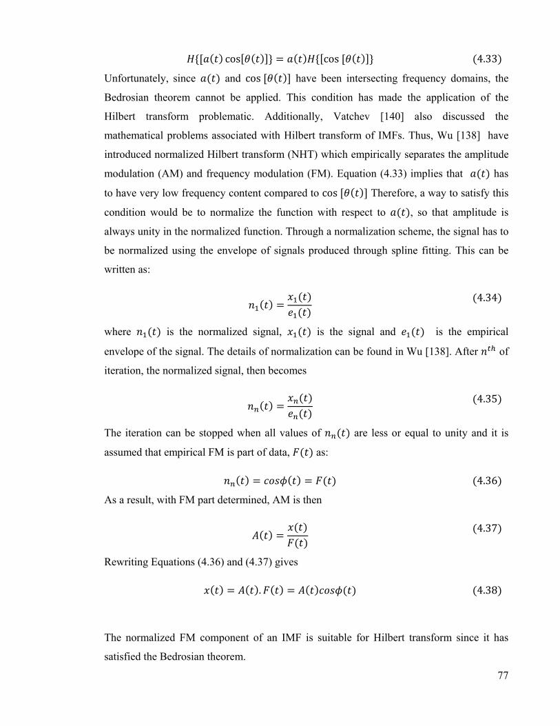
77
cos cos 4.33
Unfortunately, since and cos have been intersecting frequency domains, the
Bedrosian theorem cannot be applied. This condition has made the application of the
Hilbert transform problematic. Additionally, Vatchev [140] also discussed the
mathematical problems associated with Hilbert transform of IMFs. Thus, Wu [138] have
introduced normalized Hilbert transform (NHT) which empirically separates the amplitude
modulation (AM) and frequency modulation (FM). Equation (4.33) implies that has
to have very low frequency content compared to cos Therefore, a way to satisfy this
condition would be to normalize the function with respect to , so that amplitude is
always unity in the normalized function. Through a normalization scheme, the signal has to
be normalized using the envelope of signals produced through spline fitting. This can be
written as:
4.34
where is the normalized signal, is the signal and is the empirical
envelope of the signal. The details of normalization can be found in Wu [138]. After of
iteration, the normalized signal, then becomes
4.35
The iteration can be stopped when all values of are less or equal to unity and it is
assumed that empirical FM is part of data, as:
4.36
As a result, with FM part determined, AM is then
4.37
Rewriting Equations (4.36) and (4.37) gives
. 4.38
The normalized FM component of an IMF is suitable for Hilbert transform since it has
satisfied the Bedrosian theorem.

78
4.2.5.3.3 Direct Quadrature (DQ)
Additionally, Huang et al. [141] also applied the direct quadrature method to the
normalized IMFs to get an exact instantaneous frequency. This proposed method eschews
any Hilbert transform by means of a 90 degree shift of phase angle. After the normalization
the FM signal produced, , is the carrier part of the signal. By assuming the signal to be
a cosine function, its quadrature is given as:
1 4.39
Using the arctangent function we can calculate the phase angle and defined simply as:
1
4.40
Instantaneous frequency can be defined as the derivative of the phase function from
Equation (4.40)
4.2.5.3.4 Teager Energy Operator (TEO)
The alternative method to compute instantaneous frequency is the energy operator
(TEO) [142]. A distinctive advantage of TEO is its outstanding localization property, a
property unsurpassed by any other method. For instance, in determining the location of
leaks and other features in pipeline system time localization plays an important part. The
TEO is totally based on differentiations without involving integral transforms. For
example, taking Newton’s law of motion for an oscillator with mass, and spring constant
states that
0 4.41
the solution of the signal is of the form acos . The sum of kinetic and
potential energy is the system’s total energy , given by:
12
12
12 4.42
where , then an energy operator is defined as:

79
4.43
With constant frequency and amplitude we will have
4.44
By manipulating the two terms in Equation (4.44), we have
4.45
As a result, one can obtain both the frequency and amplitude with the energy operator.
4.2.5.4 Recent Development
One of the major drawbacks of the original EMD is the mode mixing, which is
defined as a single IMF either consisting of signals of widely disparate scales, or a signal of
a similar scale residing in different IMF components. As a result, it renders the EMD
algorithm unstable. In order to alleviate these problems, Deering [143] have proposed a
masking approach in order to prevent any lower frequency signal to be included in the IMF
and appropriately extract the intermittent components. Masking adds a component with
known frequency higher than frequency of the component that is to be extracted and later
subtracts it out to restore the actual result returned by EMD. The advantage of this method
is prevented by the presence of the higher frequency signal which will be extracted before a
lower frequency oscillation mode from the data. However, it is difficult to select the
appropriate masking signal that going to be used in the analysis hence this strategy requires
a priori knowledge of the temporal signature of components which is seldom available to
analyst.
Another solution to the problem with mode mixing and also working to reduce the
end effect, Ensemble Empirical Mode Decomposition (EEMD) was proposed by Wu and
Huang [138]. . EEMD is a noise assisted data analysis method which introduces finite
white noise to the signal. The idea is to corrupt the data with known noise where in this
case the white noise and subject to the EMD to achieve a split of the signal into various
frequency bands. Generally, EEMD working by taking ensemble mean of a number of

80
IMF’s extracted from EMD to the original data with the addition of different white noise
series each time. While the noise has been added for the individual IMFs for every trial, it
will be produce very noisy results. However, the ensemble mean of a number of
corresponding IMFs will leave only the signal as a collection of white noise cancels each
other out in a time space ensemble mean [121] . By an ensemble mean, as the number of
ensemble member, N increases the effect of the added white noise with standard deviation,
ε, the noise decreases as given by:
√ 4.46
where is defined as the different between standard deviation of the original data and the
sum of corresponding the IMFs. The proposed EEMD method can be given as follows
[121] :
(i) Add white noise series to the data.
(ii) Decompose the data with added white noise into IMF’s.
(iii) Repeat step (i) and (ii) again and again, but with different white noise series each time.
(iv) Calculate the ensemble means of the decomposition for each IMF as the final result.
As shown by Flandrin [144] EMD method to be a truly dyadic filter bank when applied to
the white noise. Therefore, the principle of EEMD is relatively straight forward since it
utilizes the scale separation principle of the EMD. Furthermore, as the data is already
separated into dyadic frequency bands, this significantly reduces the chance of mode
mixing across widely disparate time scales.
4.3 Numerical simulations to test leak detection algorithm
In order to show the efficiency of the empirical mode decomposition and the associated
Hilbert spectrum, let us validate on a simple relevant example. Consider a simple sine wave
with one frequency suddenly switching to another frequency with the presence of a Dirac
type impulse at a certain time. The impulse represents the irregularity in the signal which

81
can be considered as the reflection of the leaks or feature in the pipeline system. This signal
which has two different frequencies and is defined by the Equation (4.47):
sin 2 0 0.5sin 2 0.25 0.5 1.0 4.47
where and have the value of 80Hz and 20Hz respectively. This signal has been
selected in order to show the ability of the EMD to separate the different frequency
components as well as to identify the irregularities present in the signal. Figure 4-10 shows
the time domain of the signal along with its Fourier spectrum.
Figure 4-10: Time domain (top) and frequency spectrum (bottom) of example signal .
As we can notice from Figure 4-10 (bottom), the two frequencies components are well
presented in the Fourier spectrum however it fails to detect the spike of the irregularity in
the signal.
4.3.1 EMD analysis
The empirical mode decomposition, when applied to the signal yields six IMF’s (IMF1-
IMF6) as shown in Figure 4-11 with the last component indicating the residual.
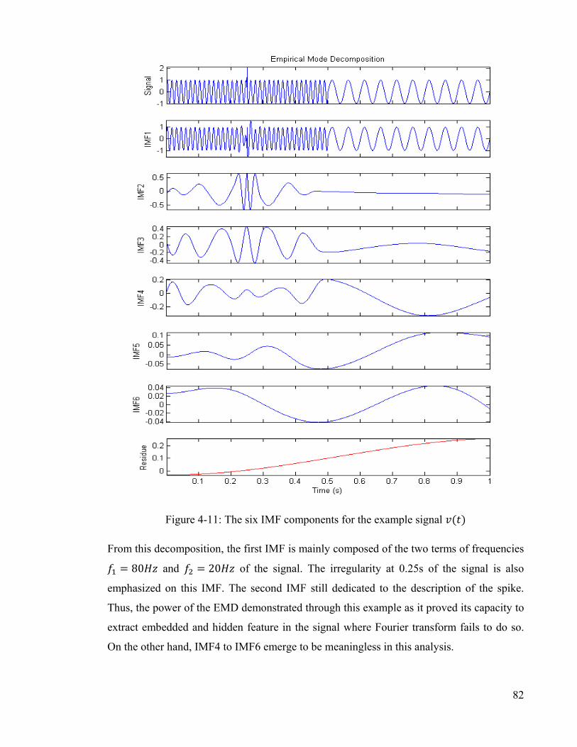
82
Figure 4-11: The six IMF components for the example signal
From this decomposition, the first IMF is mainly composed of the two terms of frequencies
80 and 20 of the signal. The irregularity at 0.25s of the signal is also
emphasized on this IMF. The second IMF still dedicated to the description of the spike.
Thus, the power of the EMD demonstrated through this example as it proved its capacity to
extract embedded and hidden feature in the signal where Fourier transform fails to do so.
On the other hand, IMF4 to IMF6 emerge to be meaningless in this analysis.

83
From this analysis, some more observations can be extracted. At each sifting iteration, it
indicates that the EMD picks out the highest frequency oscillation of the signal. It also
guarantees to always be a positive frequency, since each IMF is symmetric with respect to
its local mean. Moreover, the residue is a monotonic function from which no more IMF’s
can be extracted. The purpose of the sifting process was to obtain the monocomponent set
of functions that have well-behaved Hilbert transforms, so we have to deduct their
meaningful instantaneous frequency. As a result, it is now possible to represent the result in
the Hilbert spectrum (HS). Figure 4-12 shows the HS of IMF1-IMF3 of the test signal.
Figure 4-12: Hilbert spectrum of IMF1-IMF3 of the signal
The plot provides a high resolution time frequency representation and gives the details
about the nature of the sine wave as well as the impulse. These two frequencies can be
exactly determined with accurate time duration. The discontinuity that appears in the
impulse is well localized in time. Moreover, there is little, if any leakage, at the
discontinuity and the frequency switch point which could have been caused by EMD
method itself.

84
4.3.2 Comparison with the others signal analysis methods
After processing the signal with the Hilbert Huang transform, it is useful to analyze the
same signal through other available methods to compare their strengths and weaknesses.
Figure 4-13 shows the spectrogram of corresponding to STFT at different window
sizes
Figure 4-13: Spectrogram of at different window size
For the STFT, a random window size has been chose that is one quarter (N/4) of the signal
length. As we can see, a large time window will lead to a good frequency resolution and
poor time resolution. In addition, the two frequency components are overlapping in the
time around the switch point and it is not true that both frequencies are present in the signal
during a short time period. Obviously, it fails to show the impulse of the signal at a certain
time. Thus, a narrow window must be applied since the impulse event being localized in
time. Now the impulse obviously present in the spectrogram as shows by Figure 4-13.
However, it implies a poor frequency resolution with a smeared average frequency range
over which the main wave’s energy resides. So that in this example, this limitation of the
STFT is underlined.
So far, the wavelet analysis is the best available non stationary and non linear data analysis.
The standard Morlet wavelet type analysis able to recognize the local frequency before and
after the switch as well as the location of the frequency switch as plotted in the Figure 4-14.
The frequency resolution is not so good but still capable of identifying the two frequency
components. However, for the Daubechies wavelet type, the scalogram shows very poor

85
frequency resolution compared to Morlet type, especially for the high frequency range.
More generally, both show the presence of the impulse at the exact time of an event.
Another observation is that the scalogram shows the leakage energy to neighboring modes.
Therefore, the choice of wavelet type plays an important role in order to get useful and
accurate results from the analysis.
Figure 4-14: Scalogram of at different wavelet types.
This relatively simple example has been used to try to underline the strengths as well as the
weaknesses of the STFT, the wavelet transform and also the Hilbert Huang transform. In
summary, a comparative summary of STFT, wavelet and HHT analyses is given in the
Table 4-1:

86
Table 4-1 : Comparison of the STFT, the wavelet and the HHT [119].
STFT Wavelet Hilbert Huang
Strength
easy to implement basis function obtained by sifting and scaling a particular function
high time-frequency resolution
uniform resolution generalized Fourier analysis with variable amplitudes and frequencies
analytic form for the result local and adaptive method in frequency analysis
non stationary data analysis non linear and non stationary data analysis
feature extraction feature extraction
Weakness
piecewise stationary of the data assumption not always justified
leakage generated by the limited length of the basic wavelet function
end effects due to spline fitting and the Hilbert transform
time-frequency resolution limited by the Heisenberg principle
non adaptive nature unable to separate signals with very close frequency
non adaptive nature unable to resolve intrawave frequency modulation
no physical meaning of some IMFs
feature extraction impossible
high frequency range observation to define local events
no mathematical formulation
4.4 Summary
A review of the most common signal analysis methods used in leak detection is established
in this chapter. The standard Fourier transform (FT) and Short-time Fourier transform
(STFT) have shown some limitations to accurately describe nonstationary time series. Its
poor time-frequency resolution, its Fourier dependence and its piecewise stationary
assumption make it difficult to use despite its easy implementation. The cepstrum has the
capacity to identify the periodic structures in the spectrum and identify the presence of the
echo. Nevertheless, the performance of cepstrum suffers by the presence of noise in the
signal. Therefore, the filtering process is necessary when dealing with cepstrum analysis. In
addition, the wavelet transform is currently the most popular signal analysis method for the
nonlinear and non-stationary signals. The shifted and scaled basis functions are the main
reason for the success of wavelets in signal processing. However, one difficulty of the
wavelet analysis is its non-adaptive nature. Once the basic wavelet is selected, one will
have to use it to analyse all the data. To overcome this drawback, Huang et al [119]
introduces a new adaptive method for analyzing nonlinear and non-stationary data. In their

87
method, empirical mode decomposition (EMD) has been utilized for instantaneous
characteristics calculation. The EMD based analyses have been shown to provide better
identification of the reflection points than the other methods. Later work will show how
these can be applied to real and modeled networks.

88
Chapter 5
Leak location in pipe networks modeled with transmission line techniques (TLM)
5.1 Introduction
As defined by Chaudhry [94], a hydraulic transient is an intermediate stage of flow from
one steady state condition to another in a pressurized pipe system. In other words, the
transient conditions are initiated whenever the steady state conditions are disturbed. This
phenomenon is called water hammer when the fluid is water. Pressure transient is
generated by sudden changes of flow conditions such as pump shutdown and starts up or
valve manoeuvres. Meanwhile oscillatory or pulsating flows generated by continuous
external excitation such as steady oscillatory flows do not count as transient flow.
It is well known that pressures generated during transient conditions should be an essential
consideration when simple pipeline systems are being designed to select pipe materials,
size wall thickness in order to sustain pressure ratings and specify surge protection devices
[145]. Therefore, the concept of propagation of a wave in a liquid within a pipeline is
required to understand the water hammer occurrence [24].
Hydraulic transient can be expressed by one dimensional, two dimensional or three
dimensional models depending on the significance of the analysed phenomenon. Generally,
hydraulic models in pipeline networks are based on the assumption of one dimensional
flow [116]. Two dimensional and three dimensional models are utilized when it is
necessary to deal with particulars case such as the calculation of unsteady-shear stress
[146] or the rapid propagation of a crack when a pipe is instantaneously loaded [147]. . In
these cases, fluid equations have to be solved using the finite volume, finite difference or a
hybrid method. Furthermore, the analysis of hydraulic transients can be performed in the
time or in the frequency domain.

89
In the past few years, many refinements and improvements have been made in accuracy
and efficacy of transient analysis. The intact process of wave propagation generated by
hydraulic transient in pipes can be modeled using various simulation approaches, including
the method of characteristics[121], bond graph modeling [147], modal analysis [148] and
the transmission line modeling technique [149-151]. Many of these would be far too
computer intensive for long lengths of pipe network. Therefore, only a one dimensional
method will be able to produce the results promptly enough where variations in only one
coordinate is allowed. This means that finite difference methods are not applicable to these
purposes. On the other hand, the mathematical complexities and difficulties can be
minimized and a clearer physical picture may thus be gained [152]. Although, the method
of characteristics is the most commonly applied way of modeling waves in pipeline
networks, the simplified transmission method is efficient and often sufficiently accurate to
model this sort of problem. One of the most suitable methods for hydraulic transient
analysis is transmission line modeling [149, 151]. In fact, transmission line modeling can
be described as a form of the method of characteristics that uses a straight (linear)
characteristic line whose properties do not change with operating condition [77].
5.2 Transmission Line Modeling (TLM)
Transmission Line Modeling is a technique, computationally very efficient, for studying a
wide range of wave and diffusion phenomena. This technique offers a flexible, versatile
and efficient modeling medium for a variety and wide class of problems in the physical
sciences in general. It belongs to the class of time domain differential methods, although
recently a frequency domain version has become available [153, 154]. The basic premise
behind TLM is that the only effect of a wave going down a lossless pipe is a delay. Left and
right propagating waves in a pipe cross without affecting each other. Each pipe segment is
merely a time delay with operations occurring at junctions and waves are moved down a
pipe without modification. Additionally, TLM can account for the way that waves
propagate and what occurs to the wave at a junction will be effected by the geometry of a
pipe (which leads to the concepts of inductance and capacitance).

90
5.2.1 A short history of TLM
TLM is a technique employed in electrical engineering that operates by establishing a
correspondence between electromagnetic field components, voltage and currents in a
transmission lines [155]. The central science of TLM is transmission line theory [156].
Resistance for electrical purposes tends to be linear, so the method will work for large
amplitude variation without modification of any parameters. The general introduction of
TLM may be found in [156]. . In addition, Auslander [121, 150] has applied TLM method
to the fluid systems on his study. The next section will give a brief description of TLM
modelling techniques.
5.2.2 The concept and formulation
Electrical circuit modelling started treating networks as transmission lines that offering the
media for waves to propagate and be scattered at junctions [157]. The TLM implementation
employed in the current study was developed from the work of Auslander [150] who
adapted and applied the wave scattering methods for response simulations of elementary
fluid lines and linear mechanical systems. Auslander [150] used bond graph depiction of
such engineering systems by their energetic connections. With the help of computer
performance nowadays, this technique offer prospect for extra variation and stylizing for
topological and junction description without excessively complicating the formation of a
mathematical model or physical interpretation. In general, the solution to the wave equation
is the sum of two bidirectional waves [149]. As the transmission lines are treated as pure
delays, it leaves all the processing to be done at the junctions. At junctions, part of waves
absorbed due to friction, part of it transmitted to other pipes and part of it reflected back in
the direction from which they came. The occurrence of absorption, transmission and
reflection are a function of the junction geometry, and other devices such as filters, valves,
etc., which there may be at the junction. Physically, this is described in a previous chapter a
degree of attenuation, transmission and reflection at each junction is verified by a standard
resistance, momentum and continuity considerations. The intensity of these effects
(reflection, absorption and transmission) depends on the admittance (reciprocal of
resistance) at the junction of each of the pipes and geometry of the feature [77]. The entire
process can be modeled using TLM approach.

91
Wylie and Streeter [158] provide an excellent reference to the derivation of a wave that can
be used to approximate pipe flow. Their book commences with the explanation of
continuity equations. Then the authors develop models of dynamic components for both
compressible and incompressible liquids that utilise lumped models of capacitance and
inertance, the fluid equivalent of inductance. The approach here is an extension of
modeling each line with lumped dynamics elements by increasing the distribution of such
properties. Furthermore, the equations used for the flow by Wylie and Streeter [158] are
almost identical to the electromagnetic equations that are related to transmission lines.
Figure 5-1 displays a pipe of length , showing upstream and downstream pressure and
flows. The upstream and downstream pressures are and respectively. Meanwhile,
and indicate the flows at the upstream and downstream respectively.
Figure 5-1: Pipe showing upstream and downstream pressure and flows.
The equations governing the effect of a wave entering a transmission line form the
following pressure and mass flow relationship can be written via transfer equation as [154]:
cosh
5.1
where A is the cross-sectional area of the pipe section and is the acoustic speed of the
pressure wave. The characteristic of admittance of a general fluid line which is defined as
the ratio of pressure to flow changes associated with a wave is given by:
5.2

92
The acoustic delay time which is the time delay for wave propagates along the transmission
line of a pipe section of length , defined as:
5.3
In the TLM method, the two components of waves (referred as u and v waves) are operated
on and tracked through the system and only added where and when the flows and pressures
are desired for observation (output) [149]. The transform between pressure and flow
variables and wave scattering variables may be written:
212
212
5.4
The inverse of Equation 5.5 can be written as:
12
12
2 2
5.5
From Equation 5.1, and substituting in terms of and and the Laplace operator, , we
obtain:
0
0
5.6
Generally, for a single transmission line with distributed capacitance and inductance, the
relationship between a wave entering and leaving can be regarded as a pure time delay due
to its length and the speed of sound in it. Since the left and right propagating waves and
are decoupled, neither one affects the other. One should appreciate that all of transmission
lines are divided into segments of equal length as a speed of sound is taken to be constant
throughout the system. Each pipe is divided up into a number of segments each of a

93
common length the number of segments is rounded to an integer number. This length is
usually the shortest length of pipe in the system. Modeling the length with longer lines may
lead to errors, but these are likely not to be noteworthy. Dividing the segmentation length
can decrease these errors, but it will increase the computation time of the simulation.
5.2.3 Waves at junctions
As discussed in the previous section, at a junction some the wave is reflected back, some of
it is absorbed and some of it is transmitted to other pipes in the network. A network
consists of a number of transmission lines connected at junctions. Additionally, the
boundary to the system must be described since it also a junction. According to Equation
5.2 the admittance of a line defines how easily a wave flows into it. The relative admittance
of each line connected to a junction will verify how incident waves divide at the junction.
The common fundamental junction used in the TLM based on the implementation of the
bond graph [150] is listed as Table 5-1 where is a maximum number of ports allowed on
a multiport junction in a given application:
Table 5-1: Common junction [149].
Code name
Number of ports Function
O 2,..., Simple junction (type zero) OR 2,..., Resistive form of the above E 1,..., Constant pressure (effort) junction
ER 1,..., Resistive constant pressure junction F 1 Constant flow junction B 1 Blocked end

94
The simplest type of junction is the O junction that refers to a perfect manifold simply
joining lines in parallel. The OR junction (read as zero R, meaning type O and resistive) is
similar but consists of lumped resistance (losses) connected with at least one of its ports.
The other junction types are for boundaries.
At the E junction, the pressure is fixed and the flow is allowed to vary (e.g. pipe open to
atmosphere). This junction pressure is defined by the user (and can be specified as a
constant or as a function of time). Any lines connected at this junction do not therefore,
interact.
Meanwhile, the ER junction is the same as the E junction with a resistance on at least one
port. At the other boundary junction, namely F junction, the pressure is allowed to vary and
the flow is specified by the user.
The B junction is a non flow junction that corresponds to total blockage such as an end cap.
The F and B type junctions may only have a single pipe connected. A general TLM scheme
would also have another type of junction for the instant gyrator or transformer [159].
Figure 5-2 shows typical arrangement of topology and dimensions of modeled circuit using
TLM scheme [159].

95
Figure 5-2: Typical topology and dimensions of modelled circuit [159].
5.2.4 User input resistance and assumptions involved in TLM
In a constant diameter pipe, a resistance which is physically would be a partial blockage,
will produce the similar effect on the wave as a junction [102]. Earlier study by the
Sheffield University research group and others [72, 96] has revealed that a leak causes a
discontinuity occurrence in the flow. This in turn provides a reflection point in the same
way as any other feature such as valve, end cap or junction.
Generally, there are three types of resistance available which can be input by the user [154,
159]. These are:
1) Linear ∆ 5.7
2) Quadratic ∆ 5.8

96
3) General ∆ 5.9
In the current study, those used in the modelling utilised quadratic resistance where the
pressure drop, ∆ is proportional to the square of the mass flow rate. Moreover, a boundary
is set up at the end of the pipe. A constant pressure boundary (open end) will cause the
wave to be reflected back with the same speed and amplitude as the incident wave, but with
opposite direction [102]. Due to fluid and wall resistances, the wave will be attenuated
somewhat before it is reflected. As reported by Brown [160] under most conditions this
attenuation can be equated to steady pressure loss, which is a function of flow Reynolds
number, the pipe geometry and the pipe roughness. This however does not hold under all
conditions, and the effects of non linear attenuation and dispersions are ignored in the TLM
analysis which this work uses.
As described by Beck [159], TLM scheme ignored the effect of dispersion. In fact, at
different frequencies, the waves will propagate down a pipe at slightly different velocities.
Meaning that the pure time delay modelling employed in the TLM will not suffice to
accurately model effects of this type. This effect is trivial for short pipes with small time
delay.
5.3 Pipe network simulation and analysis
In these simulations, the software used for modeling was a program called SUNAS
(Sheffield University Network Analysis Software) and was originally developed at
Sheffield University [154, 159]. SUNAS is a powerful, one dimensional network modeling
tool. It is based on the transmission line modeling [TLM] method to simulate pipeline
networks. One dimensional TLM can describe a flow in a pipe, and the software can cope
with up to 100 junctions with 80 lines joining them. The method and its implementation are
described in detail in a previous paper by Beck [149].
The Hilbert transform (HT) and Hilbert Huang transform (HHT) methods have been
employed in order to detect the reflection from water hammer test in a pipeline network.

97
5.3.1 Simulated Models
The first model simulated was a pipe without resistance (reflection point) as shown in
Figure 5-3. The model consists of the pipe, which is divided into two sections by the valve.
To make sure that all the systems were the same, this was actually modeled as a three pipe
network, but with negligible resistance. The design of the model was made as simple as
possible in order to validate the identification approach. Opening and closing the valve
caused water hammer pulses, which then propagate through the system. In this model, the
valve is defined as a time varying resistance, as described in Beck [149, 161]. Furthermore,
SUNAS software allows the user to input geometry, lengths and diameters of the pipes. In
all models of study, air was used as a simulated fluid. It was assumed that air has S.T.P.
properties and speed of sound is equal to 343 m/s. The inlet pressure was set to 100kPa and
the outlet to 0kPa. For all tests, the diameter of the pipe was set to 15mm. The distance
between the valve and the pressure output was set to a very small distance of 0.001m for all
models. The pressure output (pressure transducer) was located as close as possible to the
valve in order to show pressure time response signal obtained through a single sensing
device [76].
Constant pressure boundary 100 kPa
Constant pressure boundary 0 kPa
Time varying valve to create pulses
A B
1 2
1 2 30.001 m
Pressure output
Figure 5-3: Pipe network model without resistance [161].
In order to simulate a pipe network with a resistance, the second model was developed. It is
shown in Figure 5-4. By adding to the first model an additional resistance, some of the
pressure wave reflects back. This effect is similar to the effect if the leak exists in the pipe
network. By knowing the distance of the reflection point from the end of the pipe, the
location of the leak can be determined. The distance of the reflection point is calculated by
multiplying the time delay corresponding to the peak by the speed of sound in the pipe
network (a=343 m/s) and halving this value to account for the return journey. In this study,

98
to observe the consistency of the results, the location of the resistance was moved to the
different distance from the end of the pipe. As shown in Figure 5-4 is a distance from
the inlet to the valve meanwhile is the distance from resistance location to the outlet of
the pipe.
Constant pressure boundary 100 kPa
Constant pressure boundary 0 kPa
Time varying valve to create pulses
A B
1 2
1 2 3
C
4
3
Location of resistance
0.1m
Pressure output
Figure 5-4: Pipe network model with resistance.
In the simulation test, two different locations were examined; resistance at 17m and 11m
from the measuring point/valve. The value of resistance was also varied. Three cases were
considered: a pipe without resistance, small resistance and large resistance for the purpose
of analyse the effect of the resistance value to the reflection point. For the large and small
resistances (see Equation 5-8), the selected values were 300 MPa (kgs-1)-2 and 30 MPa (kgs-
1)-2 respectively.
5.3.1.1 Test A: Resistance location 11m from the end of the pipe (A=7m, B=17m and
C=11m)
Figure 5-5 shows the simulated time/pressure response. The thick solid line represents the
signal with large resistance, the dot line represents the signal with small resistance and the
dot dashed line represents the signal without resistance. As it can be seen in Figure 6-4, it
can be seen that increasing the resistance (or restriction) have number of effects. Among
them is the increase of the time constant of the system due to the fact that the larger
resistance means that the pipes take longer to empty. It is hard to recognize any features
present in the pipe network without further analysis using appropriate signal processing. It
is not clearly visible what causes the changes in the pressure wave shown in Figure 5-5. As
a result, the detection and location of reflection points are difficult in practice. Hilbert
transform (HT) and Hilbert Huang transform (HHT), as described in Chapter 4, has been
utilised to greatly improve the detection and location procedure.

99
Figure 5-5: Simulated time/pressure response of the pipeline network system.
5.3.1.1.1 The HT analysis
By using HT, the instantaneous frequency and phase angle of the original signal was
obtained. Figure 5-6 shows the instantaneous characteristics for three cases.

100
Figure 5-6: Instantaneous phase and instantaneous frequency analysis using HT for Test A.
The signal with large resistance in thin solid line (top); The signal with low resistance in
dashed lines (middle); The signal without resistance in dot dashed lines (bottom).
The top plot in Figure 5-6 shows the instantaneous phase and instantaneous frequency for
the large resistance case. As it can be seen, a slight phase change occurs at 17m from the
measuring point that corresponds to the resistance present in the network. In addition, a
reflection is obviously also present at 17m as shown by the instantaneous frequency plot.
The signal from the circuit with the large resistance shows significant phase change
compared to the signal without resistance or with a small resistance at around 17m. The
occurrence of reflection at the outlet of the pipe is not present in the large resistance case as
the flow finds it hard to pass the resistance and travel to the end of the pipe.

101
The middle plot of the Figure 5-6 shows the instantaneous characteristics of the signal with
a small resistance. It can be seen that a peak occurs at 17m which corresponds to the
location of the resistance with the magnitude of this peak is less than that produced with the
large resistance. Since the size of the resistance is small, the flow can pass through the
resistance more easily, compared to the large resistance. As a result, a second spike is also
noted at the outlet which is located at 28m from the measuring point. As the power of
pressure wave with time decays, the peaks become smaller.
The bottom plot of the Figure 5-6 shows the instantaneous characteristics of the signal
without resistance. Only one big peak can be obtained around 28m which corresponds to
the outlet of the pipe network. Since there is no resistance in the system, there is no
reflection present 17m from valve.
Observing this figure shows that the instantaneous frequency obtained using the HT shows
the reflection of the wave can be obtained from the features present such as resistance and
outlet in the pipeline network. The height of the peak can be used to define the size of
resistance. The capture of the obtained instantaneous phase shows changes to the phase
when resistance exists.
5.3.1.1.2 The HHT analysis
The best representation of the results obtained using the HHT for the given data analysis is
the Hilbert spectrum or Hilbert Huang spectrum. Firstly, the signal has been decomposed
using EMD into seven IMF as shown in Figure 5-7. Only the EMD analysis of signal with a
large resistance is shown here. The first component shows the time/pressure response while
the last one indicates the residual of the signal. Then the signal has been analysed using
HHT. As it can be seen in the Figure 5-7, the signal has been decomposed from high
frequency to low frequency.

102
Figure 5-7: The seven IMF components for large resistance signal.
Hilbert spectrum (HS) of IMF1-IMF6 for the signal with large resistance is displayed as
Figure 5-8.

103
Figure 5-8: Hilbert spectrum of IMF1-IMF6 of the signal with large resistance.
It can be seen from the Figure 5-8 that there is only one high peak occurring at the location
of the resistance, approximately at 17m. The end effect phenomenon also clearly present in
Figure 5-8. The ripple at the low frequency part of the spectrum is caused by the EMD
method, not the Hilbert transform as explained by Huang [119].
Figures 5-9 and 5-10 show the Hilbert spectrum for signals with a small leak and without a
leak respectively. Both analysis used IMF1-IMF4. The result is almost the same as with the
HT analysis where for the small leaks, the spikes appear at about 17m and 28m from the
valve or measuring point. This distance refers to resistance location and the outlet of pipe
respectively. Meanwhile for no resistance, as indicated in Figure 5-10, the peak only occurs
at the exit of the pipe. Again, the unwanted ripple shown as black dashed shape at the
bottom of Figure 5-10 is also present at the lower side frequency.
Leak

104
Figure 5-9: Hilbert spectrum of IMF1-IMF4 of the signal with small resistance.
Outlet
Leak

105
Figure 5-10: Hilbert spectrum of IMF1-IMF4 of the signal without resistance.
5.3.1.2 Test B: Resistance location 17m from the end of the pipe (A=7m, B=11m and
C=17m)
In the second test, the location of the resistance was moved from 11m to 17m from the end
of the pipe. The location of the resistance was moved in order to see if the location of the
peaks would vary according to the locations of the leaks. For the second test, the small
resistance has been used i.e. 30 MPa (kgs-1)-2. The time/pressure response for the Test B is
shown as Figure 5-11.
Outlet

106
Figure 5-11: Simulated time pressure response of the pipeline network system for Test B.
5.3.1.2.1 The HT analysis
The analysis of the signal is same as the first test which is used HT and HHT. First HT
result has been presented in this section. Figure 5-12 shows the instantaneous properties of
the original signal using the HT.

107
Figure 5-12: Instantaneous phase (top) and instantaneous frequency (bottom) analysis using
HT for Test B.
The top part of Figure 5-12 shows the instantaneous phase of the signal. The figure shows
that the phase changes at a distance of 11m from the measuring point, corresponding to the
location of the resistance. Additionally, it has the change of phase at about 28m that again
indicates the location of the pipe outlet. As it can be seen from the bottom part of the
Figure 5-12, the first peak in the instantaneous frequency occurs at a distance of 11m. The
distance of 11m corresponds to the location of the measuring point. The second peak,
which represents the outlet of the pipe, again occurs at 28m. As a result, the reflection from
the resistance and outlet can be effectively captured using HT analysis.

108
5.3.1.2.2 The HHT analysis
In the same manner as in the first case using the HHT analysis, the analysis in this section
shows the final capture of the data in the form of the Hilbert Huang spectrum. As before,
we analyse the result using HHT, this signal is decomposed into eight IMF’s using EMD
and is displayed in Figure 5-13.
Figure 5-13: Decomposed signal of Test B.

109
The simulated signal has been decomposed into eight IMF with the final component
indicating the residual of the signal. The IMF1-IMF4 have been selected for the analysis.
The result of Hilbert spectrum for Test B is shown in Figure 5-14.
Figure 5-14: Hilbert spectrum of IMF1-IMF4 of the signal with small resistance for Test B.
In Figure 5-14, the peaks at about 11m and 28m from the measuring point are clearly seen.
As in Figure 5-9, the unwanted ripple (shown as black dashed shape) is again shown in the
Hilbert spectrum. This problem has been discussed by Huang [119] and attributed to
inaccuracies introduced by the spline fitting procedure used in the algorithm.
Outlet
Leak

110
5.4 Summary
Computational modelling has been performed on simple pipeline networks using the
SUNAS software; based on TLM. The two cases analysed here show the relationship of the
peaks appearance to features in the simulated pipe network. This demonstrates, therefore,
that at least for these idealised models, using the HT and the HHT it is possible to identify
the locations of the simulated features. The analysis gives simple and clear results.
According to the results obtained, the following summary can be made. By using the HT
and the HHT analysis, the instantaneous frequency and phase of the signal can be found.
Using both methods by defining the properties of pressure wave reflections, the locations of
the discontinuities of the simulated pipeline network were found. However, in real case the
analysis will be more complicated and challenging since the data presumable buried in the
noise that presents in the signal. The simulation described in this section helps to give the
guideline for analysis as it is similar to the experimental work that will be studied in the
following chapters.

111
Chapter 6
Instantaneous Phase and Frequency for
the Detection of Leaks and Features in a
PVC Pipeline
6.1 Introduction
Water is vital for life and changing climatic conditions have led to shortage and the
restriction of water use in many parts of the world. Therefore, leakage reduction and
control have become high priorities for water supply and authorities in order to prevent the
loss of this valuable natural resource. Clearly water transmission and distribution networks
deteriorate with time [44] and the inevitable aging of pipe infrastructure results in
undesirably high leakage levels. This process is sped up by high operating pressures,
inadequate design, pipe corrosion and interference of third parties. Water that is lost after
treatment and pressurization, but before delivery to customers is lost resource, money and
energy [33].
In the recent years, many water utilities have been active in working with leakage control
programmes and have achieved the “leakage economic level (LEL)” in their distribution
networks. Their attention is now drawn to the determination and location of the occurrence
of leaks in water systems. Consequently, leak detection and location are a vital element
when managing pipeline systems. During the last decades, a number of efficient methods
have been introduced for leak detection. These methods have been described in earlier
publications by the Sheffield group [105]. For example, acoustically monitoring pipelines
to determine the occurrence of the leak, as well as the damage caused by third party
interference or other catastrophic failure. More recently, many engineers and researchers
interested using wave deflection from water hammer analysis [91] for leak detection
techniques. This occurs when a valve is closed rapidly and pressure wave is generated
through the system. When this wave encounters a feature such as a leak or a service
connection, additional reflection points are produced. Furthermore, if properly utilised, the

112
pressure history of the signal and reflected waves can be captured, which presumably
contains information on the geometry, topology and also the features in a pipeline network.
The experimental setup described in this chapter has been used to obtain pressure response
produced by sudden closure of a valve to produce transient flow for detection and location
of the leak and other features in the pipeline network. A device used to create the water
hammer pulse and at the same time acquires the data of the pressure response is located at a
single point. This device is designed to fit onto a standard UK fire hydrant and is connected
to the PC for data capture and analysis.
6.2 Description of experimental set up
Numerous techniques of creating and acquiring pressure transient have been exploited to
identify and locate the features in pipelines, including leaks. A number of researchers have
employed pumps to vary the flow in the pipe and others have used valves to change the
flow rate and pressure in the pipeline network. A sudden opening and closing of the valve
generate a pressure wave that travels along the pipeline at the speed of sound. For example,
the speed of sound the MDPE pipe was 500 / . The two well researched transient base
leak identification and location methods, direct transient analysis (sometime known as leak
reflection method (LRM)) [68, 79, 80, 82, 83] and inverse transient analysis (ITA) [69, 73,
86] have been used to detect the leak. The latter methods rely on the reverse engineering of
the system to model the wave; for this, pressure transducers are usually located some away
from the valve that picks up the wave passing given points. The ITA approach is based on
minimizing the difference between measured and simulated pressure traces. The difficulties
of ITA lie on the accuracy of modelling the transient and need to set up appropriate
boundary conditions of the pipe system. Liou [72] began the analysis reflection of the first
waves to pinpoint the features in a pipe pipeline network. Later, Brunone [82, 83] used the
transient test for leak detection in outfall pipes. The location of the leak is determined by
timing of the reflected pressure and the speed of sound.
The aim of this experimental work is to show that it is reasonably straightforward to
pinpoint and locate the leaks and other features by utilising simple, readily deployable and
mobile apparatus that using a single hydrant for access. This experimental setup has been
constructed in the Hydraulic Laboratory of the Department of Civil and Structural
Engineering, The University of Sheffield. As shown in Figure 6-1, the setup comprises 90m

113
MDPE pipe of 79mm internal diameter. In order to have a long pipe in the confined lab, the
pipe was fixed horizontally on the laboratory floor in six loops. It has been anchored in
several places along its length to prevent any longitudinal movement in the system. A
constant level upstream tank is open to atmosphere and is used as the supply reservoir and
thus provides a constant supply pressure for the system during transient flows. A variable
speed centrifugal pump was fitted at the entrance of the pipeline to create flow and pressure
in the system. The pressure and flow rates can be achieved are up to 4 bar and 10 /
respectively, by controlling the pump speed and valve opening. Furthermore, the flow was
monitored by a turbine meter and system pressure was monitored by two 10 bar pressure
transducers.
Figure 6-1: The experimental set-up at the University of Sheffield.

114
6.2.1 Signal acquisition
Generally, in water distribution systems there are not usually conveniently positioned
valves or transducers; however, there are numerous access points already fitted in the form
of hydrants. The water hammer pulses were created and acquired using a device which is
designed to fit onto a standard UK hydrant [162]. To measure the pressure transient signal a
pressure transducer is installed at the base of the device (on a standard hydrant end cap) as
depicted in Figure 6-2.
Figure 6-2: The pressure transducer attached to the hydrant.
At the top, open, end of the pipe a solenoid valve has been installed and connected with
copper piping of 12mm internal diameter and 1.6m long as shown in Figure 6-3.

115
Figure 6-3: The solenoid valve has been installed and attached to hydrant.
When the solenoid valve is energised it opens and water from the mains travels through the
hydrant and out of the open end of the pipe which is connected to the reservoir using a
flexible hose. The solenoid valve is shut when power turns off. As a result, the sudden
arresting of the flow in the solenoid creates a water hammer pulse in the copper pipe that
causes a pressure wave which propagates down the pipe then into the hydrant and hence
travels to the main pipe. Part of the pressure wave travels downstream in the main pipe and
part of it travels upstream. Every discontinuity in the pipe system causes some reflection of
the wave back towards the hydrant. As the pressure wave keeps bouncing around the pipes,
it will become weaker as a result of the friction and spreading out due to the different
characteristics frequencies in the wave travelling (and attenuating) at different rates. Figure
6-4 displays an example response from pressure transducers once the transient device has
been activated.

116
Figure 6-4: Typical pressure response as transient device activated.
The device used has several advantages. The main strength of this device is obvious as it
can both create a pressure pulse and acquire the system response data from only a single
standard access point. The device is easy to handle and operate by the operator/technician
as the test can be conducted at the existing access point (fire hydrant). The other advantage
is that it always extracts water from the pressurised system; it thus has no health or
contamination issues associated with it. Moreover, due to nature of the device that works
like a domestic tapping, the amplitude of pressure wave generated in the distribution
system is akin to that a normal user could cause; meaning that the transient pressure wave
generated by the device is unlikely to cause any damage to the system. Therefore, the
design of the device is promptly suitable to be used by the water company.
In this experiment, the pressure transducer used was a Kistler (strain gauge type) that
installed into the hydrant cap. A simple data acquisition system which captures the pressure
signal at a frequency of 10 kHz is attached to the transducer. The data is fed into a personal
computer/laptop for processing and analyzing. Data acquisition was synchronised to start
when the solenoid valve closed. A variety of the leak point is located at different places
along the pipeline with the aim of determining the effect of a change of the leak position in
the processed results, such as those shown in Figure 6-5. The leak points have a constant
diameter and can be blocked by a cap as displayed by Figure 6-6.

117
Figure 6-5: Leaking point distributed along the pipe.
Figure 6-6: The cap is removed to simulate the present of leak.
In order to simulate the leak, a small ball valve of 6mm inner diameter, which discharges
to atmosphere, has been installed at a certain distance from the inlet; this is shown in Figure
6-7.

118
Figure 6-7: Ball valve to simulate the leak.
Experiments were conducted at a steady state system operating pressure of 2 bar and
system flow rate of about 0.7 l/s. Hence the system was indicative of the lowest pressures
and higher flow rates likely to be experienced by 3-4” pipes in water distribution systems
under normal operating conditions. In order to accurately locate the feature, the wave speed
of the pipeline has to be calibrated by measuring the time taken for generated transient
wave to travel from the measurement point to the boundary of the pipeline and back to the
measurement point. From this, the speed of sound was calculated as 493 m/s. This is
similar to other experiences with PE pipe.
6.3 Analysis of Pressure Signals
As the aim of this work is to compare the effectiveness of the HT and the HHT analysis of
a pressure transient signal in order to detect and locate leaks and other features in the
pipeline systems, both simulated models and laboratory experimental data have been used
for verification. The software used for modeling was described briefly in the Chapter 5.
The set up and parameter used for simulation is same as the experiment conducted as
explained in the previous section. A series of experimental test was carried out using the
laboratory pipe facility both without a leak and with a leak located 27m from the hydrant
using a sampling rate of 10kHz.

119
6.3.1 Simulated Pressure Signal
The first TLM model simulated was a pipe without a leak. The model consists of the pipe,
which is divided into two sections by the valve (see Figure 6-8).
Constant pressure boundary 100 kPa
Constant pressure boundary 0 kPa
Time varying valve to create pulses
7 m 80 m
1 2
A B C 0.001m
Pressure output
Figure 6-8: Network model without leak.
The distance between the pressure transducer and the outlet of the pipe is 80m. The design
of the model was made as simple as possible in order to validate the identification
approach. Opening and closing this valve causes water hammer pulses, which then
propagate through the system. In this model, the valve is defined as a time varying
resistance, as described in Beck et al. [21]. In order to simulate a pipe network with a leak,
a second model was developed, shown in Figure 6-9.
In the simulated models, water was used as a simulated fluid. It was assumed that water
has S.T.P. (Standard Temperature and Pressure) properties. As the experiment used MPDE
(Medium Density Polyethylene) pipe of a diameter of 79mm, a speed of sound equal to
493 / [67] was employed similar to experimental measurement though this can vary
greatly. The inlet pressure was set to 100kPa and the outlet to 0kPa. A sampling frequency
of 10 kHz was used in this simulated model. The distance between the valve and the
pressure output was set to 0.001m. This simulates the capture of a time history of pressure
using a pressure transducer located very close to the valve. The software used also allows
the user to choose any number of flow and pressure data as the output from the system. In
the current study, the output was chosen as a single pressure output in pipe 2, at junction B
as shown in Figure 6-9.

120
Constant pressure boundary 100 kPa
Constant pressure boundary 0 kPa
Time varying valve to create pulses
7 m 27 m
1 2
A B C
53 m
D
3
Junction with leak
0.001m
Pressure output
Figure 6-9: Network model with leak at 27m from the hydrant.
By adding to the first model an additional leaking junction at 27m from the measurement
point, some of the pressure wave generated by the valve will be reflected. By knowing the
distance of the reflection point from the end of the pipe and the speed of sound that
pressure waves to travel through the medium, we can determine the location of the leak.
6.4 Results
6.4.1 The HT analysis
Figure 6-10 shows a typical signal from a simulated network. By using the HT, the
instantaneous frequency and phase angle of the original signal was obtained. Figure 6-
11(dash line) shows the instantaneous characteristics of the signal. Both instantaneous
phase and frequencies clearly highlight the presence of a reflection. The peak of the
analyzed signal matched up with the time taken for the wave to travel along the pipe
network to the reflection point and return to the measurement point. The distance of the
reflection point is calculated by multiplying the time delay corresponding to the peak by the
speed of sound in the pipe network (a=493 m/s) and halving this value to account for the
return journey.
The instantaneous characteristics of the analysis for the network with a leak positioned
approximately 27m from the measurement point are also shown in Figure 6-11(solid line).

121
A new peak is now present, which indicates a leak. The two cases analyzed above reveal
the relationship of the instantaneous characteristics in the signal and features of the
simulated pipe network. In the first case, the change of phase and peaks in the
instantaneous frequency are observed at a distance of about 80m. This distance corresponds
to the location of the pipe end. In the second case where leaking point was introduced;
additional change of phases and instantaneous frequency occur approximately 27m from
the valve.
Figure 6-10: Sampled data from the simulated pipe network.

122
Figure 6-11: Instantaneous phase (top) and instantaneous frequency (bottom) analysis using
HT of simulated networks without leak (dash line) and with a leak (solid line) located 27m from the
valve. The first experiment was conducted without the present of a leak. The data captured
by pressure transducer and the processed result using the HT of the signal without a leak is
shown as Figures 6-12 and 6-13 respectively. From the first of these, it can be seen that the
pressure in the pipeline goes up when the solenoid valve is closed also the reflections of the
pressure wave in the pipe. From Figure 6-13, the instantaneous phase and frequency show
the signature of reflection point, which occurred approximately 0.323 seconds after the
valve shut. This is the time taken for the waves to propagate along the pipeline network to
the reflection point and return to the measuring section. If this time is multiplied by the
speed of sound and divided by two, it gives 79.6m, which corresponds to the distance to the
outlet of the pipe located 80m from the measuring section, with the error of about 0.5%.
Outlet Leak
Outlet
Leak

123
Figure 6-12: Experimental pressure signal without the present of leak.
Figure 6-13: Instantaneous phase (top) and instantaneous frequency (bottom) from HT
analysis of experimental data without the present of leak.
Outlet
Outlet

124
The second experiment was conducted with the presence of a leak 27m from the measuring
point. Figure 6-14 shows the experimental pressure signal for one complete cycle of the
system. By using the HT, we can obtain the instantaneous characteristics of the signal.
Figure 6-15 shows the instantaneous frequency and phase angle of the measured signal. It
can be clearly seen in the results from the HT analysis that there are two peaks, which are
the signature of the reflection points corresponding to the leak, and the end of the pipe. The
time corresponding to the first reflection point is 0.11s which gives an analyzed length of
27.12m. Compared to the actual leak (27m from the measurement point), the error is about
0.44%. For the outlet (80m from the measurement point), the time is 0.32s which
corresponds to an analyzed length of 79.6m, giving an accuracy of about 0.5%.
Figure 6-14: Experimental pressure signal with leak located 27m from measuring point.

125
Figure 6-15: Instantaneous phase (top) and instantaneous frequency (bottom) from HT analysis of experimental data with a leak located 27m from the measuring point.
For the next two experiments leaks were introduced 35m and 74.5 from the measuring
point. The pressure signal data for these experiments are shown as Figure 6-16.
Figure 6-16: Experimental pressure signal with leak located at 35m (top) and 74.5m (bottom) from measuring point.
Leak
Leak
Outlet
Outlet

126
The signal data has again been analysed using HT and the processed results are shown as
Figures 6-17 and 6-18. As it can be seen in Figure 6-14, two peaks appear at 0.145s and
0.320s. This value corresponds to the location of the leak (35m) and also the exit of pipe
(80m) with errors of about 1.91% and 1.49% respectively. Moreover, Figure 6-18 shows
the occurrence of a reflection at 0.297s and 0.321s which also corresponds to the locations
of the leak (74.5m) and the outlet of the pipe (80m), the error is about 0.98% for the leak
and 1.06% for the outlet of the pipe. It can be noted that in Figure 6-15, the presence of
noise is also obvious; this can be filtered out using a suitable filtering method which will be
discussed in the next section.
Figure 6-17: Instantaneous phase (top) and instantaneous frequency (bottom) from HT
analysis of experimental data with a leak located 35m from the valve.
OutletLeak
LeakOutlet

127
Figure 6-18: Instantaneous phase (top) and instantaneous frequency (bottom) from HT
analysis of experimental data with a leak located 35m from the valve.
Table 6-1 summarises the results of all the tests. In general, both experimental and
simulated results confirm that the HT can provide simple and clear results, which indicate
that this analysis technique can locate leaks and features in simple pipe systems with
acceptable errors.
Table 6-1: Summary results of the tests with and without leaks using HT.
Test Analysed time (s) Corresponding
Analysed Distance (m)
Measured Distance (m) Error (%)
Leak Outlet Leak Outlet Leak Outlet Leak Outlet No Leak - 0.323 - 79.6 - 80 - 0.5
Test1 0.11 0.323 27.12 79.6 27 80 0.44 0.5 Test2 0.145 0.32 37.74 78.8 35 80 1.91 1.49 Test3 0.297 0.321 74.21 79.15 74.5 80 0.98 1.06
Outlet Leak
Outlet Leak

128
6.4.2 The HHT analysis
In this section, the signal is analysed using a newly proposed method from Huang [119];
the Hilbert Huang transform (HHT). As briefly discussed in Chapter 4, the best
representation of the results obtained using the HHT for the given data analysis is the
Hilbert-Huang spectrum (HHS). Firstly, the signal needs to be decomposed using EMD
before it can be presented in the form of the Hilbert spectrum. The processed results
presented in this section use the distance in metres for the x-axis instead of the time in
seconds as shown in the previous section. It is simple to convert from time to distance by
multiplying the time taken that wave to travel by the speed of sound divided by two. Figure
6-19 shows the eleven IMFs and their residue from the simulated signal without the
existence of a leak. The first three IMFs contain the highest frequency while higher levels
of IMF correspond to low frequencies. The offset and the basic response of the system are
in the low frequency range; these levels were therefore discarded. By selecting IMF4-IMF7
and summating them generates a pressure signal without noise. Consequently, Figure 6-20
shows the HS of the pressure response of the pipe network without a leak. As expected, it
can be seen that there is only one high peak at a location about 80m from the valve,
showing the reflection of the pipe end. Figure 6-21 shows the HS for signals of selected
IMF4-IMF7 of pipe network with a leak present. Figure 6-21 also shows a peak at about
80m, in addition, we also have a peak at approximately 27m, which corresponds to the leak
position. The analysis using HHT produced a good result for a leak and also can identify
the end point in the simulated pipeline network. Incidentally, the HS also generates
unwanted IMFs in the low frequency region, indicating a disadvantage of the EMD
method, which is not encountered by the HT.

129
Figure 6-19: The IMF’s and its residue of the simulation data.

130
Figure 6-20: HHT spectrum analysis of IMF4-IMF7 of simulated network without leak.
Figure 6-21: HHT spectrum analysis of IMF4-IMF7 of simulated network with leak located
27m from the valve.
Outlet
Outlet
Leak

131
The experimental data from the rig described above was then was analyzed using the HHT.
The signal with the leak located 27m from the measuring point was decomposed into 11
IMFs and its residue as shown in Figure 6-22. As we can see from this, IMF1 to IMF3
contain the highest frequencies (and highest energy), which is mostly noise. The other
IMFs are in the low frequency range. In addition, EMD clearly displays spatial and
temporal information from the pressure wave signal records. These features could not have
been extracted using classical Fourier transform analysis. By removing IMF1 to IMF3 and
summing IMF4-IMF8, a pressure signal without noise was generated and when compared
with original signal (as shown in Figure 6-23), it looks similar but more clean. As
explained by Flandrin et al [144], the EMD technique can be worked as the filter to remove
the noise from the data. Furthermore, Figure 6-24 shows the HS of the selected IMF. From
the results shown in the HS, clearly it can reveal the reflection points corresponding both to
the location of the leak and the end of the pipe, which are located 27m and 80m,
respectively from the measurement point.

132
Figure 6-22: The IMF’s and its residue of the experimental data.
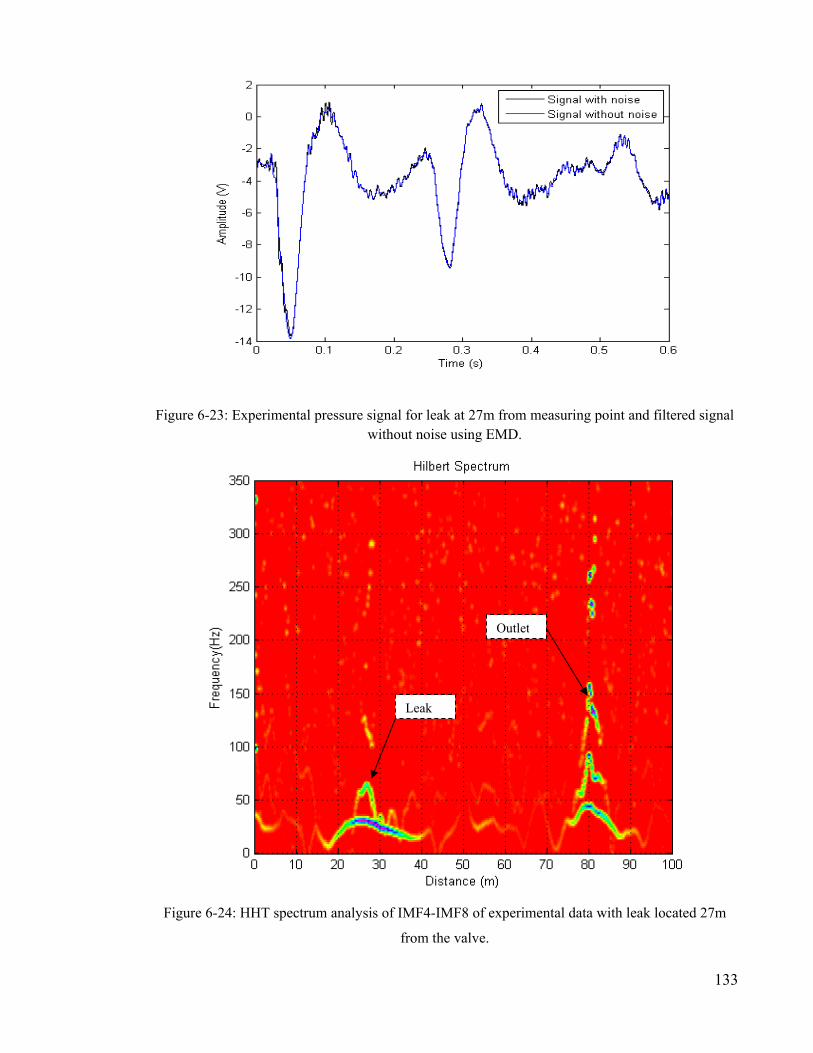
133
Figure 6-23: Experimental pressure signal for leak at 27m from measuring point and filtered signal without noise using EMD.
Figure 6-24: HHT spectrum analysis of IMF4-IMF8 of experimental data with leak located 27m
from the valve.
Outlet
Leak

134
Meanwhile, for the test of the leak that located 35m and 74.5m from the measurement point IMF4-
IMF9 have been utilized for both analysis. The processed result using HHT for the both
experiments is shown in Figure 6-25 to Figure 6-28.
Figure 6-25: Experimental pressure signal for leak at 35m from measuring point and filtered signal without noise using EMD.
Figure 6-26: Experimental pressure signal for leak at 74.5m from measuring point and filtered signal without noise using EMD.
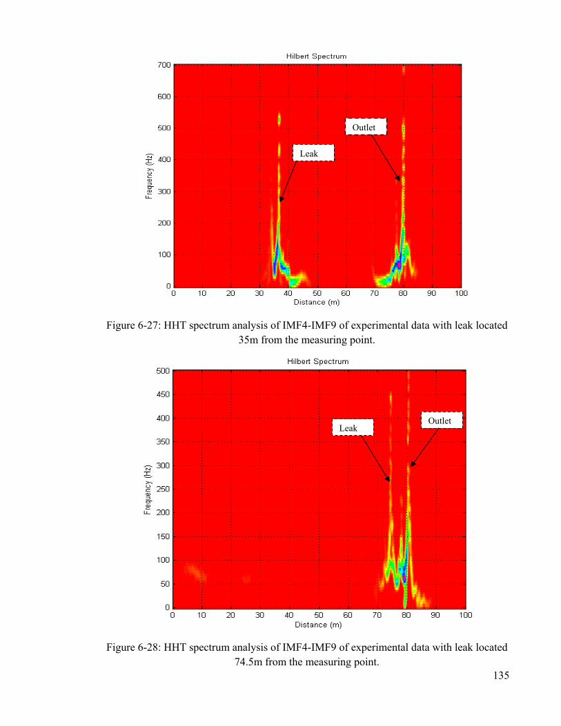
135
Figure 6-27: HHT spectrum analysis of IMF4-IMF9 of experimental data with leak located 35m from the measuring point.
Figure 6-28: HHT spectrum analysis of IMF4-IMF9 of experimental data with leak located 74.5m from the measuring point.
Leak
Leak
Outlet
Outlet

136
As shown in Figure 6-25 and 6-26 the pressure signals have been filtered using the EMD
technique to remove the noise. The reconstructed signal using IMF4-IMF9 was then
analysed using HS. The result is shown as Figures 6-27 and 6-28. As it can be seen from
the figures, the reflection corresponding to both the leak and outlet of the pipe can be
clearly captured using the HHT method. On the other hand, there is an unnecessary ripple
which still exists in the low frequency region caused by the EMD method. There is also
visible in the presence of noise. As explained by Huang [119] It is impossible to remove
all the noise that is buried in the signal.
Table 6-2 summarises the results of all of the tests. In general, both experimental and
simulated results confirm that the HHT can provide simple and clear results, which indicate
that this analysis technique can locate leaks and features in simple pipe systems with
acceptable errors.
Table 6-2: Summary results of the tests with and without leaks using HHT.
Test Analysed time (s) Corresponding
Analysed Distance (m)
Measured Distance (m) Error (%)
Leak Outlet Leak Outlet Leak Outlet Leak Outlet Test1 0.111 0.326 27.35 80.32 27 80 1.28 0.4 Test2 0.144 0.325 35.44 80.13 35 80 1.24 0.16 Test3 0.303 0.326 74.68 80.31 74.5 80 0.24 0.4

137
6.5 Summary
The instantaneous phase and frequency of pressure waves through fluid-filled pipelines
produced using both simulated and experimental signal were analyzed in order to identify
leaks and other features. These two characteristics were extracted using the HT and the
HHT.
Neither method had previously been applied in a systematic way to the problem of
identifying features in pipeline systems. The results confirmed that HT analysis can
identify features in simple pipeline systems for both simulated and experimental signals.
The features that were identified as causing a reflection were the leak and the pipe end. The
location of the leak by the HT approach was excellent with a low percentage of error.
Furthermore, the similar HHT analysis worked well to identify features if experimental
data is used.

138
Chapter 7
Comparative Study of Instantaneous
Frequency Based Methods for Leak
Detection in Pipeline Networks.
7.1 Introduction
Yorkshire Water is a water supply company servicing South Yorkshire, West Yorkshire,
the East Riding of Yorkshire, part of North Lincolnshire, most of North Yorkshire and part
of Derbyshire, in England with 1.7 million household. They provide about 1291m litres
through 31062 km of mains pipeline. The geographical position of Yorkshire Water
compared to other water companies in England and Wales is shown as Figure 7-1.
Figure 7-1: Map of water companies supply each area of England and Wales [163].

139
As reported by the UK industry regulator (OFWAT) the total daily water loss in England
and Wales due to occurrence of leakage is about more than 1.8 billion litres, or 12% of the
water that the companies put into the distribution system [27]. It will cost about £100
billion to replace all of existing pipeline networks and every customer’s supply pipe [27].
As a result, the total costs and the impact on customers’ bills would be several times higher.
As well as renewing pipelines, leak reduction can be effectively implemented by fixing
specific leaks. A variety method as explained in the Chapter 2 have been developed and
implemented by the researchers in order to pinpoint the location of the leak. However, there
a very few study that have been validated with the field data [164].
For the real systems filtering is required to remove unwanted features such as noise, trends
or frequency components prior the instantaneous frequency (IF) analysis. Many methods of
filtering could be used to remove noise; the current study utilizes the empirical mode
decomposition (EMD) filtering procedure due to nonstationary nature of the analysed data.
The data are decomposed to different levels with different frequency bands. The low levels
contain the high frequency (system noise) and high levels of this decomposition contain
low frequency elements (the basic system response in this case). Summing the signal
without the low and high frequency components allows a filtered signal to be produced.
The work presented here will demonstrate its applicability in live water distribution
networks and then compared with existing methods of analysing instantaneous frequency.
The next section discussed the leak detection scheme and tested via simulation followed by
implementation of the proposed method using field test data.
7.2 Leak detection scheme outline
7.2.1 Implementation
The proposed leakage detection methods have been evaluated by the following steps:
• Use a pressure transient signal from field tests conducted on a field operator
training site and real distribution network.
• Decompose the data into set of monocomponent signals, i.e IMF by using EMD, as
described in section 4.2.5 in Chapter 4.

140
• Filter the signal by discarding some of the irrelevant IMF.
• Compute instantaneous frequencies using Hilbert transform (HT), Normalized
Hilbert transform (NHT), Direct Quadration (DQ), Teager Energy Operator (TEO)
and Cepstrum as described in section 4.2.5.3 in Chapter 4.
• From extracted signals calculate the distance to the leak and other features.
• Compare and evaluate results of the analysed methods.
The operation procedures can be summarized in the flowchart as shown in Figure 7-2.
Figure 7-2: The operation procedure of the proposed method.
7.2.2 Numerical simulations to test leak detection algorithm
To evaluate the proposed method consider following synthetic signal:
7.1
Where and are the background signal and the impulse representing reflection of
leaks or features, respectively. The background signal can be chosen as:

141
x t sin 0.027πt sin 2 0.027π t π/2 sin 4 0.027πt 7.2
Figure 7-3(a) shows 300 samples of x(t) and Figure 7-3(b) indicates two spikes with an
amplitude of 0.1, with v(t) at instants 120 and 240 respectively. The combinations of these
are shown in Figure 7-3(c). The algorithm has been applied to the simulated signal; it has
yielded five IMFs as shown in Figure 7-4. Applying all methods proposed to IMF1,
instantaneous frequency has been calculated and the results are shown in Figure 7-5. As it
can be seen, for the clean signal, all methods indicate the reflection at the correct
occurrence times.
Figure 7-3: The synthetic signal with the present of artificial impulse.

142
Figure 7-4: The 5 IMFs component with its residue for the )()()( tvtxts +=
Figure 7-5: The simulated signal with instantaneous frequency by HT, NHT, DQ,
TEO and Cepstrum.
For further analysis, white noise has been added, and hence Equation 7.1 becomes:

143
7.3
The white noise is normally distributed with mean 0 and standard deviation 1 with signal-
to-noise ratio (SNR) is 40, as generated using MATLAB version 7. The signal has then
been decomposed into eleven IMFs as shown in Figure 7-6. IMF1-IMF7 consists of most
of the noise. IMF8-IMF10 have been chosen for further analysis while the rests of IMF’s
are considered irrelevant. Using the same method of calculating instantaneous frequency as
described above, the results of this analysis are shown as Figure 7-7. Again, all the method
successfully detects the reflection at their correct occurrence time. The TEO method shows
the worst result since it only performs well in the absence of noise (as previously explained
by Huang [141]). EMD also works as a filter bank [144] hence it is possible to remove all
unnecessary noise in the signal.

144
Figure 7-6: The 11 IMFs component with its residue for the

145
Figure 7-7: The simulated signal with noise and instantaneous frequency contribution by
HT, NHT, DQ, TEO and Cesptrum.
7.3 Experimental method
A simple device that produces mild pressure transient which has been used previously in
laboratory work was utilized here, collects the resultant pressure signal and analyses the
data using the method described in the previous section. With the help and support of
Yorkshire Water, the initial test has been conducted at Yorkshire Water’s field operators
training site located in Esholt, Bradford followed by the test at real distribution system in
Yorkshire.
7.3.1 Field site 1 -Field operators training site, Esholt
This test site does not serve customers but is connected to and fed with water from a live
system. Figure 7-8 shows the view of the site test together with their schematic map
pipeline arrangement. In Figure 7-8(c), the red lines are pipes of different materials and
size, the blue circles are hydrants, the triangles are leak points and the small black line are
valves, which have been distributed in different positions around the network. The supply
into the system is from the bottom left of Figure 7-8(c). The large numbers of valve help
the operator to reconfigure the system easily in order to isolate the different sections of the

146
network. In addition, the measurement and pressure transient creation points are UK
standard hydrants. This training site was designed to allow the new staff to learn about leak
detection and identification. The section of the system tested in this work is shown in
Figure 7-9.
a) b)
c)

147
Figure 7-8: Yorkshire Water’s field operators training site in Esholt, Bradford: (a) Google
maps view (red circle); (b) View of pipeline path; (c) Schematic map pipeline arrangement.
Figure 7-9: Field site 1 test setup with distances of all features relative to the testing hydrant is shown.
On this system, instead of a pump to provide pressurized water to the system, mains water
supplies are used. The pipe used consists of a 90mm PVC main. The lengths of the pipe
section are short compared to the real systems; therefore, it is expected to provide more
complex signal changes than real systems, although potentially less signals degradation. In
this test, a periodic closing and opening of a solenoid valve that connected to a hydrant
through a short metal pipe which was used to generate hydraulic transient events, this is
shown in Figure 7-10. The use of small diameter pipe limits the peak transient pressure
such as that system damage is unlikely. The measurement device was placed onto a
hydrant. Therefore, the pressure signal acquired through a pressure transducer, is sampled
through a PC at 10kHz. In order to ascertain the constant pressure in the system and to
ensure that an acceptable pressure was maintained in the network, a visible pressure gauge

148
was fitted closed to the measuring section. The assembled device used in the test was
shown in Figure 7-11.
Figure 7-10: The device used to generate and collect the pressure transient signal.
Figure 7-11: The complete measurement setup during the test.

149
7.3.1.1 Test results
All the pipes in this test were PVC and the calibrated speed of sound was 540 / . As
illustrated in Figure 7-9, the leaks can be opened and closed at the locations marked A and
B via tapings, which discharge into the ground. For this series of test, the system pressure
was 6 bar. The solenoid valve and pressure transducer are installed at the testing hydrant as
shown in Figure 7-10. Figure 7-12 shows the recorded transient after each of the four tests
run. As we can see from the figure, the closing valve occurs approximately at t = 0.18s. The
pressure rises rapidly immediately after the valve is closed and then drops. This shows that
the transient signal produced is transmitted and reflected throughout the pipe system, all the
while being attenuated through both friction and various features in the pipe network. The
analysis of the signal starts immediately after the valve is closed.
Figure 7-12: Sampled data from field site 1 test.
The signal then is decomposed using EMD, which yields nine IMFs from a high to a low
frequency as shown in Figure 7-13. IMF1 and IMF2 consist mostly of the noise while IMF
9 and the residue contain the basic response of the signal. Therefore, all of these IMFs have
been removed. By selecting IMF3-IMF8 and summating them generates a pressure signal
without noise. The comparison between original signal and the filtered signal is depicted as
Figure 7-13.

150
Figure 7-13: The IMF’s and its residue of field site 1 test.

151
Figure 7-14: Original signal (left) and filtered signal (right) of the raw data from field site 1
test.
This remaining, filtered, signal was analysed using the instantaneous frequency techniques
introduced earlier. It will be seen that these produce peaks that can be identified as various
features in the system, like valves, hydrants, corners and of course, the leak. These are
shown in Figure 7-15.

152
Figure 7-15: Instantaneous frequency analysis of IMF3-IMF8 using HT,NHT,DQ,TEO and
Cesptrum and Taghvaei [105] of the field site 1 test.
The peaks shown in the analysed results correspond to the time taken by the wave to travel
along the pipe and return back to measuring point (after wave speed calibration). The
distance of the leak and features from the source of transient (H2) can be estimated simply
by multiplying the time delay data corresponding to the each peak by the calibrated speed
of sound (i.e. a=540m/s) in the pipe system and halving this value to account for the return
a)
b)
c)
d)
e)
f)

153
journey. The results then can be compared with the distances on the schematic map. The
summary of this analysis along with the errors can be found in the Table 7-1.
Table 7-1: Summarised result of the field site 1 test data for different instantaneous
frequency analysis.
Features Analysed Distance (m) Measured
Distance (m)
Error (%)
HT NHT DQ TEO Cepstrum HT NHT DQ TEO Cepstrum
Valve 1 (V1) 3.48 3.51 3.67 3.97 3.86 3.50 0.49 0.29 4.91 13.43 10.31 Hydrant 2(H2) 7.16 7.02 7.29 7.18 6.86 7.00 2.21 0.29 4.14 2.57 -2.00 Leak A (LA) 10.29 10.53 10.58 10.64 - 10.70 3.83 1.59 1.12 -0.56 - Valve 2 (V2) 15.04 15.04 15.07 15.04 - 15.00 0.27 0.27 0.47 0.27 - Leak B (LB) 17.50 17.23 17.23 17.15 18.01 17.70 1.13 2.66 2.66 -3.11 1.75 Corner (C) 23.11 22.92 22.49 25.00 21.11 22.00 5.05 4.18 2.23 13.64 -4.05 Hydrant 3(H3) - 26.86 26.78 27.19 24.73 25.50 - 5.33 5.02 6.63 -3.02 Hydrant 4(H4) 28.35 29.02 29.02 31.18 32.08 30.00 5.50 3.27 3.27 3.93 6.93 Valve 3 (V3) 37.75 37.80 37.85 38.39 38.66 37.00 2.03 2.16 2.30 3.76 4.49
It can be seen that almost methods can identify leak A (LA) and leak B (LB) which occur
approximately at t= 0.0396s (hence 10.7m) and t= 0.0655s (hence 17.7m) respectively from
the measurement point with an acceptable of error (within -0.56% to 3.83%). The HT
method can capture most of the features but at the same time produces unnecessarily
spikes. This suggests that the instantaneous frequency calculated can capture the
discontinuity produced by the leak and other features. The improvement of HT called NHT
and DQ [141] are able to identify most of the features within a reasonable accuracy. The
result produced by both NHT and DQ is clearer compared to HT.
The TEO method gives an acceptable result but with very small amplitude peak at corner
(C) and a high percentage error for valve 1 (V1) compared to measured distance. This is
probably caused by the wave profiles having intra wave modulations or harmonic
distortions. TEO is also very sensitive to the presence of the noise [141] which will affect
the accuracy of the analysis. The combination of EMD and Cepstrum gives the worst result
since it failed to locate the reflection from both leak A and valve 2. It also produces other
spurious peaks, which may lead to miscalculation the distance of the features or false
results. Furthermore, as explained by Huang [119] the common problem with the EMD is

154
the frequent appearance of mode mixing, which is defined as either a single IMF consisting
of widely disparate scales, or a signal residing in different IMF components.
As a comparison, the results produced are also compared with the method proposed by
Taghvaie [105] where they used the combination of wavelet and cepstrum. The result is
shown in Figure 7-15(f). Most of the features are detected except for the hydrant H3 and it
also produced a small reflection of leak A (LA). It also produces irrelevant reflections,
which may be caused by the noise present in the filtered data using orthogonal wavelet
transform (OWT). It should be noted that this method is very susceptible to the wavelet
levels selected.
This has shown that features and leak points along a pipeline can be determined by filtered
signal via EMD and analysis of instantaneous frequency, with only a small error in
distance. The NHT and DQ methods perform the best while the rest of the instantaneous
frequency methods also produce acceptable results.
7.3.2 Field site 2 –Yorkshire Water’s distribution network (Roach Road,
Sheffield)
A second field test is presented from Yorkshire Water’s distribution network in Roach
road, Sheffield. The Google map view and also the schematic map of the test site are shown
as Figure 7-16. The pipeline is constructed of cast iron with a nominal diameter of 4 inches.
Measured average system pressure was 4 bars. A pinhole leak of 10mm diameter at a flow
rate of 0.3 l/s is present in the system. The test is conducted from hydrant 1 (H1) marked in
Figure 7-16. The leak is located about 29m from the hydrant 1 (H1) as identified by the
Yorkshire Water operator. Again, a simple data acquisition system which captured the
resultant pressure signal at a frequency of 5 kHz was used as shown in Figure 7-17. The
same data collection and analysis technique described in the previous section were used
here. The transient event however, was generated by rapidly opening and closing a small
solenoid valve fitted to the testing hydrant (see Figure 7-18). To accurately locate each
feature or leak, the wave speed of the pipeline has to be calibrated by measuring the time
taken for generated transient wave to travel from the measurement point to the boundary of
the pipeline and back to the measurement point. The time/pressure history is shown in
Figure 7-19. The theoretical speed of wave propagation is 1310 / while the determined

155
value was 1300 / . It is anticipated that the leak and other features will provide
reflections and can be detected by instantaneous frequency analysis.
Figure 7-16: Field site 2 configuration: (a) Google maps view (marked as red); (b)
Schematic map pipeline arrangement.
a)
b)

156
Figure 7-17: Typical connection of pressure transducer to the hydrant.
Figure 7-18: Connection of solenoid valve to hydrant to generate pressure transient.
The time/pressure history of the test is shown in Figure 7-19.

157
Figure 7-19: Sampled data from field site 2 test.
7.3.2.1 Test results
After filtering this data through EMD and scaling with respect to the speed of sound and
the time for a reflected wave, the instantaneous frequency characteristics are used to try to
pinpoint the location of leak and other feature i.e. hydrant for this case. The analysed
results are shown as Figure 7-20. In order to confirm the location of the leak, the test was
also conducted at hydrant 2 (H2) as marked in Figure 7-16 (b). For both analyses the
summation of IMF4-IMF8 has been used. The processed results and summarized results are
shown in Figure 7-21. The analyses of field test 2 are summarised in Table 7-2. From the
analysis, it is confirmed that the location of the leak is located approximately at 29m from
hydrant 1 (H1) or 33m from hydrant 2 (H2). Hydrant 2 (H2) and Hydrant (H3) are also
correctly located by this analysis. HT, NHT and DQ produce the best results with only
small error while TEO and cepstrum analysis capable of determining the location of the
leak but with only a small amplitude peak in the processed result. The combination of
wavelet and cepstrum [105] analyses generate the worst result since it produces some
irrelevant peak.

158
Figure 7-20: Instantaneous frequency analysis of IMF3-IMF8 using HT,NHT,DQ,TEO and
Cesptrum and Taghvaei [105] of the field site 2 test data using hydrant 1 (H1).
a)
b)
c)
d)
e)
f)
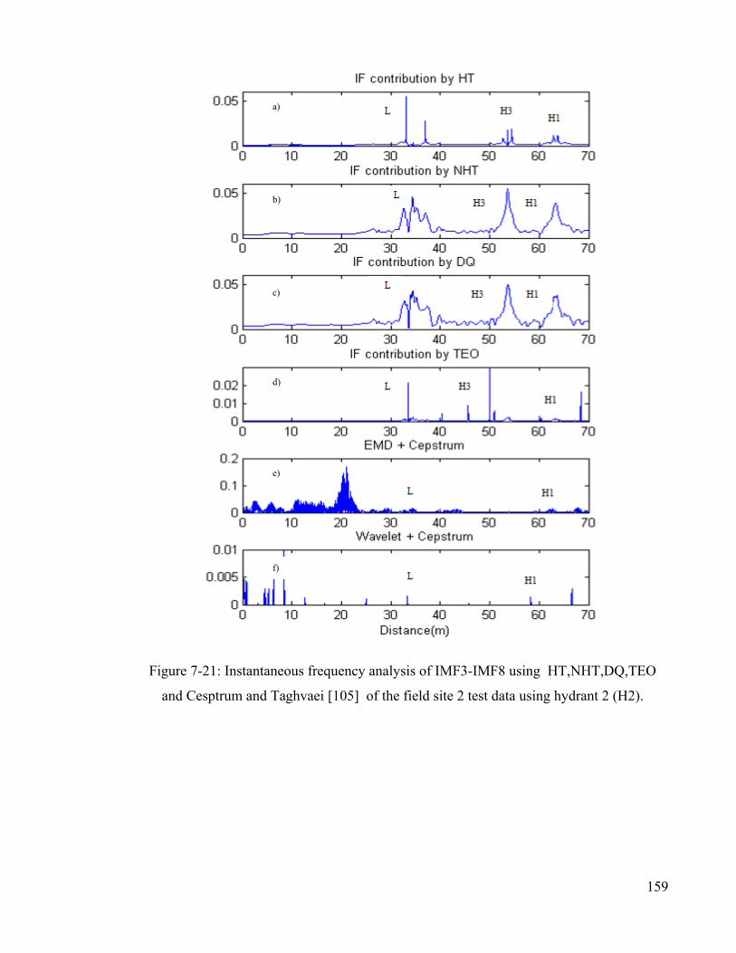
159
Figure 7-21: Instantaneous frequency analysis of IMF3-IMF8 using HT,NHT,DQ,TEO
and Cesptrum and Taghvaei [105] of the field site 2 test data using hydrant 2 (H2).
a)
b)
c)
d)
e)
f)

160
Table 7-2: Summarised result of field site 2 test data for different instantaneous frequency
analyses: (a) Results of analysis using hydrant 1 (H1); (b) Results of analysis using hydrant
2 (H2).
(a)
Features Analysed Distance (m) Measured
Distance (m)
Error (%)
HT NHT DQ TEO Cepstrum HT NHT DQ TEO Cepstrum
Leak(L) 29.93 29.32 29.41 29.09 28.99 29 3.21 1.10 1.41 0.31 0.03 Hydrant 2 (H2) 62.01 61.33 61.26 61.23 61.2 62 0.02 1.08 1.19 1.24 1.29
Hydrant 3(H3) 115.5 114.3 114.4 114.4 112.8 115.4 0.09 0.95 0.87 0.87 2.25
(b)
Features Analysed Distance (m) Measured
Distance (m)
Error (%)
HT NHT DQ TEO Cepstrum HT NHT DQ TEO Cepstrum
Leak(L) 33.05 32.7 32.7 33.48 34.48 33 0.15 0.91 0.91 1.45 -4.48 Hydrant 3 (H3) 53.59 53.69 53.69 53.72 - 53.4 0.36 0.54 0.54 0.60 -
Hydrant 1(H1) 62.89 63.47 63.05 63.15 62.37 62 1.44 2.37 1.69 1.85 -0.60
7.3.3 Field site 3 –Yorkshire Water’s distribution network (East Bank
Road, Sheffield)
The next test was again conducted within a Yorkshire Water’s distribution network located
at East Bank road, Sheffield. A Google map view and schematic map of the site are shown
in Figure 7-22. The pipeline is constructed of 4 inches nominal diameter cast iron with a
leak of size of 3.5 l/s located approximately 40m from hydrant 2 (H2). The hydrants and
leak locations are shown as “H” and “L” respectively in Figure 7-22(b). There is also a
pressure reducing valve (PRV) located near to the hydrant 1 (H1). In this case, the testing
was conducted from hydrant 2 (H2). There is also a pressure reducing valve (PRV) located
near to the hydrant 1 (H1).

161
Figure 7-22: Field site 3 test configuration: (a) Google maps view (marked as red); (b)
Schematic map pipeline arrangement.
The procedure of data collection, data processing and calibration technique is the same as
the previous test field test. The data was sampled at 5 kHz. The theoretical speed of wave
propagation in this pipe is 1310 m/s and the calibrated value was 1090 m/s. This difference
a)
b)
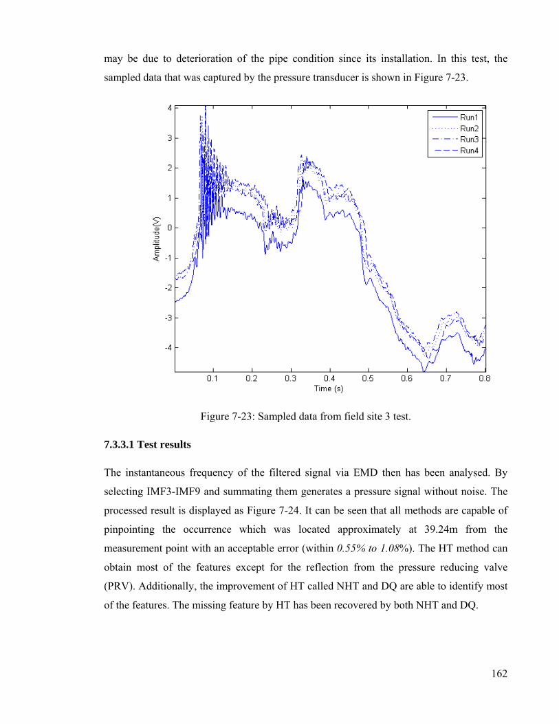
162
may be due to deterioration of the pipe condition since its installation. In this test, the
sampled data that was captured by the pressure transducer is shown in Figure 7-23.
Figure 7-23: Sampled data from field site 3 test.
7.3.3.1 Test results
The instantaneous frequency of the filtered signal via EMD then has been analysed. By
selecting IMF3-IMF9 and summating them generates a pressure signal without noise. The
processed result is displayed as Figure 7-24. It can be seen that all methods are capable of
pinpointing the occurrence which was located approximately at 39.24m from the
measurement point with an acceptable error (within 0.55% to 1.08%). The HT method can
obtain most of the features except for the reflection from the pressure reducing valve
(PRV). Additionally, the improvement of HT called NHT and DQ are able to identify most
of the features. The missing feature by HT has been recovered by both NHT and DQ.

163
Fig 7-24: Instantaneous frequency analysis of IMF3-IMF9 using
HT,NHT,DQ,TEO and Cesptrum and Taghvaei [105] of the field site 3 test data.
The TEO method gives a satisfactory result, but it also produces other irrelevant peaks,
which may lead to miscalculation the distance of the features. The combination of EMD
and Cepstrum gives the worst result since it only shows the peak corresponding to the leak
point. It also indicates the hydrant 3 (H3) and junction 2 (J2) with a very small amplitude
peak and fails to locate the rest of features in the network. The processing result again is
compared with the analysis conducted by Taghvaie [105]. They utilized the combination of
wavelet and cepstrum in order to detect the reflection of leak and features in the pipeline
a)
f)
e)
d)
c)
b)

164
network. The result is shown in Figure 7-24(f). Their proposed method is capable of
detecting and locating most of the features except for hydrant1 (H1). On the other hand,
some irrelevant peaks were also produced. This was probably caused by the noise that was
still present in the filtered data using OWT. The summary of this analysis along with the
errors can be found in the Table 7-3.
Table 7-3: Summarised result of the field site 3 test data for different instantaneous
frequency analysis.
Features Analysed Distance (m) Measured
Distance
(m)
Error (%)
HT NHT DQ TEO Cepstrum HT NHT DQ TEO Cepstrum
Leak(L) 40.22 39.46 39.57 39.68 39.567 40 0.55 1.36 1.08 0.81 -1.08
Junction 1(J1) 137.4 137.3 137.2 137.2 - 138.5 0.79 0.87 0.94 0.94 -
Hydrant 1(H1) 141.3 141 140.8 140.6 - 142 0.49 0.70 0.85 1.00 -
Hydrant 3(H3) 154.9 155.7 155.8 156.2 156.7 154 0.58 1.10 1.17 1.43 1.75
PRV - 165.9 165.8 166 - 160 3.69 3.63 3.75 -
Junction 2(J2) 203.1 204.9 205.2 205.4 205.7 204 0.44 0.44 0.59 0.67 0.83
Hydrant 4(H4) 300.9 297.6 297.7 297.9 - 293.4 2.56 1.43 1.47 1.53 -
7.4 Summary
The instantaneous frequency of pressure waves through fluid-filled pipelines of a real life
system signal was analyzed in order to identify leaks and other features. Firstly, collected
transient data was decomposed and filtered by empirical mode decomposition (EMD).
Then, a range of different methods of calculating instantaneous frequency such as HT,
NHT, DQ and TEO have been evaluated and compared. The analysis using EMD and
Cesptrum also has been studied. Neither method had previously been applied in a
systematic way to the problem of identifying features in real life pipeline systems. The
features that were identified as causing a reflection were elements such as: a leak, a
hydrant, a junction, a corner, a valve and a pressure reducing valve. The processed results
confirmed that the instantaneous frequency calculation by NHT and DQ analysis can reveal
most of the features and for these cases, Cepstrum analysis gives the worst result.

165
Chapter 8
Conclusions and Future works
8.1 Overview
Leak detection and location in pipelines are essential to prevent economic and energy
losses, ensure safety and control environmental problems. Therefore, effective techniques
for leak detection are very important when managing pipeline systems. During the last
decades, a number of efficient methods have been introduced for leak detection.
The work described in the first part of the present study represents new techniques based on
the analysis of a pressure wave. These methods could be more effective and accurate in
detecting leakages that the current cross correlation, wavelet and cepstrum techniques being
postulated. The innovation of these techniques is the analysis of instantaneous phase and
instantaneous frequency. Both instantaneous characteristics are calculated using the Hilbert
Transform (HT) and the Hilbert-Huang Transform (HHT).
The second part of the study presents a comparative study of instantaneous frequency
analysis techniques based on pressure transients recorded within a live water distribution
network. The aim is to explore and compare a proposed method of analysing non-stationary
data called Empirical Mode Decomposition (EMD) for instantaneous characteristics
calculation for leak detection.
Additionally, a section of simulated modeling was conducted in order to identify the
features in a simple pipeline network. Computational modelling has been performed on
simple pipeline network using SUNAS software that based on transmission line modelling
(TLM). The software used allows the user to input geometry, lengths and diameters of the
pipes. The presence of a lumped resistance in the simulated network cause a reflection in
the signal which can be referred to features in the system.

166
8.2 Conclusions
All the work reported here, uses transient analysis of water hammer waves for leak
detection. Water hammer occurs when a valve is closed rapidly and pressure wave is
generated through the system. When this wave encounters a leak or other features such as a
junction, a valve or a hydrant, additional reflection points are produced and can be captured
using a single pressure transducer. All features are located by measuring the period of time
which the pressure wave takes to propagate from the measuring point to the features and
back. The main conclusions drawn from the research can be summarised as follows:
For the simulation test using SUNAS software, the instantaneous frequency and phase of
the signal could be found using the HT and the HHT analysis. Using both these methods to
define these properties in the pressure wave history, the locations of the discontinuities of
the simple simulated pipeline network were found. It was also discovered that the size of
the resistances affects the values of the instantaneous properties. Change in the resistance
location showed the pattern of change in the peaks locations. In the HHT analysis, the
unwanted ripple also present at the low frequency part of the spectrum which is seen in the
EMD method, but not in the Hilbert transform.
The leak detection research has been extended to transient test in the laboratory. The
experimental setup in the department of civil engineering is used to capture the pressure
transient signals in the pipeline with and without a leak. Both simulated and experimental
pressure signals were used to evaluate the performance of these transforms. The proposed
technique predicts satisfactorily the location in simple pipeline systems as it can detect and
locate the leak up to error of 0.5%. Moreover, experimental application of the proposed
technique has shown great potential to locate a leak. From the three different location of
leak test conducted the error was in the range of 0.44% to 1.96%. Meanwhile for the outlet
of pipes, the error is about 0.5% to 1.49%. Therefore, analysis of the experimental tests
corroborates the simulated test results when the HT and the HHT analysis are used. The
analysis using HT and HHT can be considered the first application to leak detection and
location. In addition, this technique has many advantages over the presently available
techniques, such as simplicity of application, ease to use and thus can be considered
economical.

167
In the experimental work, a simple device was developed that attaches onto a UK standard
hydrant in order to produce the pressure transient in the test rig. Fitted to the hydrant end cap,
there was also a pressure transducer which was in contact with the water in the hydrant.
This device provides both pressure creation and acquires system response data from a
single, standard access point. Turning off the power to the solenoid valve causes it to shut.
This suddenly stops the water in the copper pipe creating a water hammer pulse that travels
down the pipe, into the hydrant and hence into the main pipe.
Furthermore, the research was extended to present a comparative study of instantaneous
frequency analysis techniques based on pressure transients recorded within a live water
distribution network. It has shown that EMD is an effective method to remove the noise
that can mask the signal in many real cases. The innovation of this technique is the analysis
of Instantaneous Frequency (IF). The instantaneous frequency of the filtered signals are
analysed using the Hilbert Transform (HT), the Normalized Hilbert transform (NHT),
Direct Quadrature (DQ), Teager Energy Operator (TEO) and Cepstrum.
In the first test at Esholt training ground, it can be seen that almost methods can identify
both leaks with an acceptable of error (within -0.56% to 3.83%). The HT method can
capture most of the features but at the same time produces unnecessarily spikes. The
improvement of HT called NHT and DQ are able to determine most of the features within a
reasonable accuracy and clearer compared to HT. Meanwhile, TEO method is also very
sensitive to the presence of the noise which will affect the accuracy of the analysis. The
combination of EMD and Cepstrum gives the worst. In the second and third test are
presented from Yorkshire Water’s distribution network, Sheffield. In the second test, all the
proposed method capable of detect and locate the leak within acceptable of error. Using the
test from first hydrant, the error was 0.03% to 3.21%. Meanwhile, the test from second
hydrant the error was in the range of -4.48% to 0.15%. Moreover, in the third test, it is
found that all methods are able to determine the occurrence of leak with an acceptable error
(within 0.55% to 1.08%). Additionally, the NHT and DQ are able to identify most of the
features with the missing feature by HT has been recovered by both NHT and DQ. As a
comparison, the results produced are also compared with the method proposed by
Taghvaie. The result is shown that most of the features are detected but at the same time it

168
also produces irrelevant reflections, which may be caused by the noise present in the
filtered data using orthogonal wavelet transform (OWT).
The proposed method has shown that features and leak points along a pipeline can be
determined by filtered signal via EMD and analysis of instantaneous frequency, with only a
small error in distance. The NHT and DQ methods perform the best while the rest of the
instantaneous frequency methods also produce acceptable results.
8.3 Recommendations for future work
The current study has tried to develop a new methodology in the field of signal processing
for leak and feature detection in the pipeline network based on transient signal analysis. In
order to extend the use of the proposed method, there is several advancement in the current
state of art that needs to take place. Some of this is to improve the technique and some of it
is to commercialise it. Following is a list of recommendations to enhance the accuracy of
the leak detection system:
• Several pressure transducers in different places can be used to capture the change
of pressure over a large portion of a water distribution system, instead of using only
a single pressure transducer. It is important in order to monitor the system or to get
vital information to improve leak identification. • The analysis of a simulated signal using TLM can be replaced by more complicated
and accurate models which incorporate better physics. Furthermore, the application
to other fluid flows of bigger diameter can be examined with the existing models in
order to observe the effect of leak on changes of pressure wave in different size of
pipe at different complexity. • Large scale networks with complicated systems and a wider range of operational
conditions have to be explored. An extended series of field trials needs to be
conducted, and improve the system and analysis of the signal. • As empirical mode decomposition (EMD) is still new in signal analysis study, it
needs to be improved to produce the more accurate and satisfying results. One of
the main problems is the uncertainties about which IMFs are relevant in any EMD

169
process, which contributes to the overall difficulty in trying to physically interpret
the IMFs of signals. Therefore, in order to improve the overall EMD process, some
form of mathematical expression is necessary to discriminate between relevant and
irrelevant IMFs.

170
References
1. Global water supply and sanitation assessment 2000 report. 2000, WHO and UNICEF: New York, USA.
2. McKenzie, R., Seago, C., Assessment of real losses in potable water distribution systems: some recent developments. Water Science and Technology: Water Supply, 2005. 5(1): p. 33-40.
3. Misiunas, D., Failure monitoring and asset condition assessment in water supply systems, in Industrial Electrical Engineering and Automation Department. 2005, Lund University: Lund.
4. Pelletier, G., Modeling water pipe breaks-three case studies. Journal Water Resources Planning Management, 2003. 129(2): p. 115-123.
5. Khomsi, D., Reliability Tester for Water-Distribution Networks. J. Comput. Civ. Eng., 1996. 10(1): p. 10-19.
6. Weimer, D., Water loss management and techniques. Technical report, DVGW, The German Technical and Scientific Association for Gas and Water, 2001.
7. Sanks, R.L., Water transport section: Water storage, transport and distribution, in Encyclopedia of Life Support Systems (www.eolss.net), Y. Takahasi, Editor. 2005, EOLSS: Oxford, UK. p. 18.
8. Wang, J. and A. Atrens, Analysis of service stress corrosion cracking in a natural gas transmission pipeline, active or dormant? Engineering Failure Analysis, 2004. 11(1): p. 3-18.
9. Saegrov, S., et al., Rehabilitation of water networks: Survey of research needs and on-going efforts. Urban Water, 1999. 1(1): p. 15-22.
10. Deteriorating buried infrastructure management challenges and strategies. 2002, United States Environmental Protection Agency: Washington DC, USA. p. 37.
11. Makar, J.M., Desnoyers, R. and McDonald, S.E., Failure modes and mechanisms in gray cast iron pipe, in Underground Infrastructure Research. 2001, NRC Institute for Research in Construction; National Research Council Canada: Kitchener, Ontario. p. 1-10.
12. Cathodic protection. 2010 [cited 2010 10 September]; Available from: http://www.peterboroughutilities.ca/Water/Construction_Projects/Cathodic_Protection.htm.
13. Colombo, A.F., Energy use and leaks in water distribution systems, in Department of Civil Engineering. 2004, University of Toronto: Toronto.
14. Lambert, A.O., and Hirner, W., Losses from water supply systems: standard terminology and recommended performance measures. International Water Association (IWA), 2000.
15. Farley, M., and Trow, S., Losses in Water Distribution Networks- A Practitioner's Guide to Assessment, Monitoring and Control. 2003, IWA Publishing: London.
16. Alegre, H., Baptista, J.M., Cabrera Jr E., Cubillo, F., Duarte, P., Hirner, W., Merkel, W., and Parena, R., Performance Indicators for Water Supply Services - Second Edition. 2006, IWA Publisher: London.
17. Farley, M., Wyeth, G., Zainuddin, M.G., Istandar, A., and Singh, S., The Manager's Non-Revenue Water Handbook: a Guide to Understanding Water Losses, N. van Dijk, Raksakulthai, V., Kirkwood, E., Editor. 2008, Ranhill and USAID.
18. Burn, S., Desilva, D., Eiswirth, M.,Speers, A. and Thoronton, J., , Pipe leakage-Future challenges and solutions, in Pipes Wagga Wagga. 1999: New South Wales, Australia p. 1-18.
19. Lambert, A.O., International report: Water losses management and techniques. Water Science and Technology: Water Supply, 2002. 2(4): p. 1-20.

171
20. Wolfe, T.F., Underground leakage and its relation to mains and services. Journal of American Water Works Association, 1923: p. 400-404.
21. Ramos, H., Reis, C., Ferreira, C., Falcão, C., Covas, D. Leakage control policy within operating management tools. in 6th Computing and Control for the Water Industry (CCWI) 2001. De Montfort University, Leicester.
22. AWWARF, Distribution system performance evaluation. Denver, CO : AWWA, 1995. 23. Friedman, M., Radder, L., Harrison, S., Howie, D., Britton, M., Boyd, G., Wang, G.,
Gullick, R., LeChevallier, M., Wood, D., Funk, J., Verification and control of pressure transients and intrusion in distribution systems. Water Intelligence Online © IWA Publishing, 2005.
24. Walski, T.M., Chase, D.V., Savic, D.A., Grayman, W., Beckwith, S., Koelle, E., Advanced water distribution modeling and management. 2003, Waterbury, CT USA: Haestad Press. 751.
25. LeChevallier, M.W., Gullick, R.W., Karim, M.R., Friedman, M. Funk, J.E., The potential for health risks from intrusion of contaminants into the distribution system from pressure transients. Journal od Water and Health, 2003. 1: p. 3-14.
26. The potential for health risks from intrusion of contaminants into the distribution system from pressure transients. 2003, United States Environmental Protection Agency: Washington DC, USA.
27. Waste not, want not – making the best use of our water. 2011 [cited 2011 9 August]; Available from: www.ofwat.gov.uk/publications/focusreports/prs_inf_demand.pdf.
28. Makar, J.M., Kleiner, Y., Maintaining water pipeline integrity, in AWWA Infrastructure Conference and Exhibition. 2000, NRC Institute for Research in Construction; National Research Council Canada: Baltimore, Maryland. p. 14.
29. Colombo, A.F. and B.W. Karney, Energy and costs of leaky pipes toward comprehensive picture. Journal of Water Resources Planning and Management, 2002. 128(6): p. 441-450.
30. Water distribution network leakage in the UK. 2010 [cited 2011 12 February]; Available from: http://www.ciwem.org/knowledge-networks/panels/water-supply--quality/water-distribution-network-leakage-in-the-uk.aspx.
31. Farley, M., Non revenue water- international best practice for assesment, monitoring and control, in 12th Annual CWWA Water, Wastewater and Solid Waste 2003: Atlantis, Paradise Island, Bahamas.
32. Thornton, J.L., A. Progress in practical prediction of pressure: leakage, pressure: burst frequency and pressure: consumption relationships in Proceedings of IWA Specialised Conference 'Leakage 2005'. 2005. Halifax, Nova Scotia, Canada.
33. Leak detection. [cited 2011 5 April]; Available from: http://www.water.ca.gov/wateruseefficiency/leak/.
34. Lai, C.C., Unccounted for water and economics of leak detection. Water Supply, 1991. 9(3,4): p. IR1-1-IR1-8.
35. Comparison of European Water and Wastewater Prices. 2010 [cited 2011 20 January]; Available from: http://www.bdew.de/internet.nsf/id/DE_VEWA-Survey_summery_Comparison_of_European_Water_and_Wastewater_Prices/$file/_12_seiter_vewa_studie_bdew_ENGL_V2.pdf.
36. Mamlook, R. and O. Al-Jayyousi, Fuzzy sets analysis for leak detection in infrastructure systems: a proposed methodology. Clean Technologies and Environmental Policy, 2003. 6(1): p. 26-31.
37. Security of Supply Report 2006-2007 [cited 2011 5 February]; Available from: http://www.ofwat.gov.uk/regulating/reporting/rpt_sos_2006-07secofsupplymain.pdf.
38. Office of Water Services: Leakage and Water Efficiency. 2000 [cited 2010 19 January]; Available from: http://www.nao.org.uk/publications/9900/leakage_and_water_efficiency.aspx.

172
39. Pilcher, R., Hamilton, S., Chapman, H., Ristovski, B., and Strapely, S., Leak location and repair guidance notes., in International Water Association. Water Loss Task Forces: Specialist Group Efficient Operation and Management. 2007: Bucharest, Romania.
40. Tafuri, A.N., Locating leaks with acoustic technology. American Water Works Association 2000. 92: p. 57-66.
41. Covas, D., H. Ramos, and A.B. de Almeida, Standing Wave Difference Method for Leak Detection in Pipeline Systems. Journal of Hydraulic Engineering, 2005. 131(12): p. 1106-1116.
42. Warda, H.A., I.G. Adam, and A.B. Rashad, A Practical Implementation of Pressure Transient Analysis in Leak Localization in Pipelines. ASME Conference Proceedings, 2004. 2004(41766): p. 2193-2200.
43. Zhang, J., Designing a cost-effective and reliable pipeline leak-detection system. Pipes and Pipelines International, 1997. 42(1): p. 20-26.
44. Hunaidi, O., Wang, A., Bracken, M., and T. Gambino, Fricke, C. , Detecting Leaks in Water Distribution Pipes. Arab Water World, 2005. 29(4): p. 52-55.
45. Heitbrink, W.A., Earnest, G. S., Mickelsen, R. L., Mead, K. R. and D’Arcy, and J. B., Evaluation of leakage from a metal machining center using tracer gas methods: A case study. American Industrial Hygiene Association Journal, 1999. 60(6): p. 785-788.
46. Stampolidis, A., et al. Detection of leaks in buried plastic water distribution pipes in urban places - a case study. in Advanced Ground Penetrating Radar, 2003. Proceedings of the 2nd International Workshop on. 2003.
47. Nakhkash, M. and M.R. Mahmood-Zadeh. Water leak detection using ground penetrating radar. in Ground Penetrating Radar, 2004. GPR 2004. Proceedings of the Tenth International Conference on. 2004.
48. Seung-Yeup, H., et al. An experimental study on a ground-penetrating radar for detecting water-leaks in buried water transfer pipes. in Antennas, Propagation and EM Theory, 2003. Proceedings. 2003 6th International SYmposium on. 2003.
49. Hamilton, S., Hartley, D., Misconceptions around acoustic leak detection, in Water21- Magazine of the International Water Association. 2008, IWA Publishing. p. 54-56.
50. Puust, R., et al., A review of methods for leakage management in pipe networks. Urban Water Journal, 2010. 7(1): p. 25-45.
51. Farley, M., Finding "difficult' leaks. Water 21, 2008(9.6): p. 24-25. 52. Fuchs, H.V. and R. Riehle, Ten years of experience with leak detection by acoustic signal
analysis. Applied Acoustics, 1991. 33(1): p. 1-19. 53. Brennan, M.J., Y. Gao, and P.F. Joseph, On the relationship between time and frequency
domain methods in time delay estimation for leak detection in water distribution pipes. Journal of Sound and Vibration, 2007. 304(1-2): p. 213-223.
54. Hunaidi, O. and W.T. Chu, Acoustical characteristics of leak signals in plastic water distribution pipes. Applied Acoustics, 1999. 58(3): p. 235-254.
55. Brunone, B., Ferrante, M. Leak analysis in pipes using transients. in Second Annual Smeinar on Comparative Urban Projects. 2000. Rome, Italy.
56. Tan, G., et al. Research on Bypass-valve and its Resistance Characteristic of Speed Regulating PIG in Gas Pipeline. in Measuring Technology and Mechatronics Automation (ICMTMA), 2011 Third International Conference on.
57. Zheng, H. and E. Appleton, Dynamic characteristics of a novel self-drive pipeline pig. Robotics, IEEE Transactions on, 2005. 21(5): p. 781-789.
58. Mergelas, B., and Henrich, G., Leak locating method for precommissioned transmission pipelines: North American case studies, in Leakage 2005. 2005: Halifax, Canada.
59. Chastain-Howley, A., Transmission main leakage: how to reduce the risk of a catastrophic failure, in Leakage 2005. 2005: Halifax, Canada.
60. Hough, J.E., Leak testing of pipeline uses pressure and acoustic velocity. Oil & Gas Journal, 1988. 86(47): p. 35-41.

173
61. Liou, C.P., Mass imbalance error of waterhammer equations and leak detection. Journal Name: Journal of Fluids Engineering; (United States); Journal Volume: 116:1, 1994: p. Medium: X; Size: Pages: 103-109.
62. Parry, B., MacTaggart, R., Toerper, C, Compensated volume balance leak detection on a batched LPG Pipeline, in OMAE-Volume V-B, Pipeline Technology. 1992, ASME: New York. p. 501-507.
63. Stafford, M., Williams, N., Pipeline leak detection study. Health and Safety Executive-Offshore Technology Report (OTH 94 431), 1996.
64. Whaley, R.S., Reet, J.V., Nicholas, R.E., A tutorial on computer based leak detection methods, in PSIG Annual Meeting. 1992, Pipeline Simulation Interest Group: Texas, USA.
65. Zhang, J., Statistical pipeline leak detection for all operating conditions. Pipeline & Gas Journal, 2001: p. 42-45.
66. Farmer, E., Kohlrust, R., Myers, G., and Verduzco, G., Leak detection tool undergoes field test. Technology - Oil & Gas Journal, 1988. December(19): p. 48-53.
67. Thorley, A.R.D., Fluid transient in pipeline systems: 2nd Edition. 2004, London: Professional Engineering Publishing Limited.
68. Jönsson, L., Interaction of a hydraulic transient with a leak in a pipe flow, in 14th Australasian Fluid Mechanics Conference. 2001: Adelaide University, Adelaide, Australia.
69. Liggett, J.A. and L.-C. Chen, Inverse transient analysis in pipe networks. Journal of Hydraulic Engineering, 1994. 120(8): p. 934-955.
70. Colombo, A.F., Lee, Pedro, and Karney, Bryan W., A selective literature review of transient-based leak detection methods. Journal of Hydro-environment Research, 2009. 2(4): p. 212-227.
71. Silva, R.A., et al., Pressure wave behaviour and leak detection in pipelines. Computers & Chemical Engineering, 1996. 20, Supplement 1(0): p. S491-S496.
72. Liou, C.P., Pipeline Leak Detection by Impulse Response Extraction. Journal of Fluids Engineering, 1998. 120(4): p. 833-838.
73. Vitkovsky, J.P., A.R. Simpson, and M.F. Lambert, Leak detection and calibration using transients and genetic algorithms. Journal of Water Resources Planning and Management, 2000. 126(4): p. 262-265.
74. Vítkovský, J.P., Simpson, A. R. and Lambert, M. F., Leak detection and calibration using transients and genetic algorithms. Journal of Water Resources Planning and Management, 2000. 126(4): p. 262-265.
75. Wang, X.J., et al., Leak detection in pipelines using the damping of fluid transients. Journal of Hydraulic Engineering, 2002. 128(7): p. 697-711.
76. Mpesha, W., Leak detection in pipes by frequency response method. 1999, University of South Carolina: USA.
77. Al-Shidhani, I., S.B.M. Beck, and W.J. Staszewski, Leak monitoring in pipeline networks using wavelet analysis. Key Engineering Materials ; VOL. 245-246 ; 5. International conference on damage assessment of structures (DAMAS 2003), Southampton (United Kingdom), 1-3 Jul 2003 ; PBD: 2003, 2003: p. page(s) 51-58.
78. Ferrante, M. and B. Brunone, Pipe system diagnosis and leak detection by unsteady-state tests. 1. Harmonic analysis. Advances in Water Resources, 2003. 26(1): p. 95-105.
79. Jönsson, L., Hydraulic transients as a monitoring device, in Technical report. 1995, Dept. of Water Resources Engineering, University of Lund: Lund, Sweden.
80. Covas, D., and Ramos, H. Leakage detection in single pipelines using pressure wave behaviour. in Proceedings of Water Industry Systems: Modelling and Optimization Applications, CCWI' 99. 1999. Exeter, UK: CWS.
81. Wylie, E.B. and V.L. Streeter, Fluid Transients. 1982, Michigan: FEB Press. 82. Brunone, B., Transient test-based technique for leak detection in outfall pipes. Journal of
Water Resources Planning and Management, 1999. 125(5): p. 302-306. 83. Brunone, B. and M. Ferrante, Detecting leaks in pressurised pipes by means of transients.
Journal of Hydraulic Research, 2001. 39(5): p. 539-547.

174
84. Pudar, R.S. and J.A. Liggett, Leaks in pipe networks. Journal of Hydraulic Engineering, 1992. 118(7): p. 1031-1046.
85. Kapelan, Z., Savic, D., and Walters, G., A hybrid inverse transient model for leakage detection and roughness calibration in pipe networks. Journal of Hydraulic Research, 2003a. 41(5): p. 481-492.
86. Covas, D., Ramos, H., Brunone, B. and Young, A., Leak detection in water trunk mains using transient pressure signals: Field tests in Scottish Water, in 9th International Conference on Pressure Surges. 2004, BHR Group: Chester, UK. p. 185-198.
87. Ivetic, M.V., and Savic, D.A., Practical implications of using induced transients for leak detection. Journal of Urban and Environmental Engineering, 2007. 1(1): p. 36-43.
88. Tang, K.W., Karney, B.W., Brunone, B. Leak detection using inverse transient calibration and GA - some early successes and future challenges. in Computing and Control in the Water Industry (CCWI). 2001. Leicester, UK.
89. Covas, D., et al. Water Pipe System Diagnosis by Transient Pressure Signals. in Water Distribution Systems Analysis Symposium 2006. 2006. Cincinnati, Ohio, USA: ASCE.
90. Saldarriaga, J., Implementation of the Hydraulic Transient and Steady Oscillatory Flow with Genetic Algorithms for Leakage Detection in Real Water Distribution Networks. ASCE Conf. Proc., 2006. 247(40941): p. 52.
91. Mpesha, W., S.L. Gassman, and M. Hanif Chaudhry, Leak detection in pipes by frequency response method. Journal of Hydraulic Engineering, 2001. 127(2): p. 134-146.
92. Ferrante, M. and B. Brunone, Pipe system diagnosis and leak detection by unsteady-state tests. 2. Wavelet analysis. Advances in Water Resources, 2003. 26(1): p. 107-116.
93. Lee, P.J., et al., Frequency Domain Analysis for Detecting Pipeline Leaks. Journal of Hydraulic Engineering, 2005. 131(7): p. 596-604.
94. Chaudhry, M.H., Applied Hydraulic Transients (2nd Edition). 1987: Litton Educational Publishing Inc. Van Nostrand Reinhold Co.
95. Lee, P.J., et al., Experimental verification of the frequency response method for pipeline leak detection. Journal of Hydraulic Research, 2006. 44(5): p. 693-707.
96. Beck, S.B.M., et al., Pipeline Network Features and Leak Detection by Cross-Correlation Analysis of Reflected Waves. Journal of Hydraulic Engineering, 2005. 131(8): p. 715-723.
97. Ferrante, M., B. Brunone, and S. Meniconi, Wavelets for the Analysis of Transient Pressure Signals for Leak Detection. Journal of Hydraulic Engineering, 2007. 133(11): p. 1274-1282.
98. Young, R.K., Wavelet theory and its applications. 1993, Boston: Kluwer Academic Publishers.
99. Stoianov, I., Karney, B. W., Covas, D., Maksimovic, C., and Graham, N. . Wavelet processing of transient signals for pipeline leak location and quantification. in 6th Conference on Computing and Control for the Water Industry (CCWI). 2001. Leicester, UK.
100. Meniconi, S., et al., Small Amplitude Sharp Pressure Waves to Diagnose Pipe Systems. Water Resources Management, 2011. 25(1): p. 79-96.
101. Lighthill, J., Waves in Fluids. 2001, Cambridge: University Press. 102. Beck, S.B.M., and Staszewski, W.J., Cepstrum analysis for identifying reflection points in
pipeline networks, in 9th International Conference Pressure Surges. 2004, BHR Group: Chester, U.K.
103. Bogert, B.P., Healy, M.J.R., Tukey, J.W., The quefrency alanysis of time series for echoes: Cepstrum, pseudo-autocovariance, cross-cepstrum, and saphe cracking. Time Series Analysis, 1963: p. 209-243.
104. Taghvaei, M., S.B.M. Beck, and W.J. Staszewski. Leak detection in pipeline with use of Cepstrum method. in 16th International Conference on Pipeline Protection. 2005.
105. Taghvaei, M., S.B.M. Beck, and W.J. Staszewski, Leak detection in pipelines using cepstrum analysis. Measurement Science and Technology, 2006. 17(2): p. 367-372.

175
106. Wang, H., et al., Measurement and simulation of pressure wave attenuation in upward air-water bubbly flow. International Journal of Heat and Fluid Flow, 2000. 21(1): p. 104-111.
107. Colombo, A., Karney, B. W., Pipe breaks and the role of leaks from an economic perspective. Water Supply, 2003. 3(1-2): p. 163-169.
108. Vitkovsky, J.P., Stephens, M.L., Lee, P.J., Simpson, A.R., Lambert, M.F. The detection and location of leakage, blockage and air pockets using radar-based techniques. in Australian Water Association SA Branch Regional Conference. 2003. Adelaide, Australia: Australian Water Association.
109. Misiunas, D., M. Lambert, and A. Simpson. Transient-Based Periodical Pipeline Leak Diagnosis. in Water Distribution Systems Analysis Symposium 2006. 2006. Cincinnati, Ohio, USA: ASCE.
110. Taghvaei, M., S.B.M. Beck, and W.J. Staszewski, Leak detection in pipeline networks using low-profile piezoceramic transducers. Structural Control and Health Monitoring, 2007. 14(8): p. 1063-1082.
111. Daniel, A.R. Longitudinal and transverse wave motion. 2004 [cited 2010 8 October]; Available from: http://www.acs.psu.edu/drussell/Demos/waves/wavemotion.html.
112. Burnett, G.C. How we make shape and sound. 1999 [cited 2010 14 March]; Available from: http://www.gregandmel.net/burnett_thesis/2_3.htm.
113. Daniel, A.R. Waves in dispersive medium. 2004 [cited 2010 10 October]; Available from: http://www.acs.psu.edu/drussell/Demos/Dispersion/dispersion.html.
114. Duan, H., Investigation of factors affecting transient pressure wave propagation and implications to transient based leak detection methods in pipeline systems, in Department of Civil and Environmental Engineering. 2011, The Hong Kong University of Science and Technology: Hong Kong.
115. Stephens, M., Simpson, A.R., Lambert, M.F., and Vítkovský, J.P., Field measurement of unsteady friction effects in a trunk transmission pipeline. World Water Congress, ASCE, 2005. 173(19).
116. Covas, D.I.C., Inverse transient analysis for leak detection and calibration of water pipe systems modelling special dynamics effects, in Department of Civil and Environmental Engineering. 2003, Imperial College of Science, Technology and Medicine: London.
117. Oppenheim, A.V., Schafer, R.W., Discrete-time signal processing. 3 ed. 2009, London: Prentice Hall.
118. Dowling, M.J. Application of non-stationary analysis to machinery monitoring. in Acoustics, Speech, and Signal Processing, 1993. ICASSP-93., 1993 IEEE International Conference on. 1993.
119. Huang, N.E., et al., The empirical mode decomposition and the Hilbert spectrum for nonlinear and non-stationary time series analysis. Proceedings of the Royal Society of London. Series A: Mathematical, Physical and Engineering Sciences, 1998. 454(1971): p. 903-995.
120. Hadjileontiadis, L.J., A novel technique for denoising explosive lung sounds. Ieee Engineering in Medicine and Biology Magazine, 2007. 26(1): p. 30-39.
121. !!! INVALID CITATION !!! 122. Bjerkas, M., Wavelet transforms and ice actions on structures. Cold Regions Science and
Technology, 2006. 44(2): p. 159-169. 123. Staszewski, W.J., Wavelets for Mechanical and Structural Damage Detection. In series
Studia i Materialy, Gdansk, Monograph No. 510/1469/2000, Polish Academy of Sciences Press (IMP-PAN). 2000.
124. Qian, S., Chen, D., Joint Time-Frequency Analysis: Methods and Applications. 1996, New Jersey: Prentice Hall.
125. Wheeler, J.A., Zurek, W.H., Quantum theory and measurement. 1983, New Jersey: Princeton University Press.
126. Polikar, R. The wavelet tutorial. 2001 [cited 2009 15 December]; Available from: <http://users.rowan.edu/~polikar/wavelets/wttutorial.html>

176
127. Randall, R.B., Frequency analysis. 3rd ed. 1987, Copenhagen: Bruel and Kjaer. 128. Norton, M.P., Fundamental of noise and vibration analysis for engineering. 1989,
Cambridge: University Press. 338-342. 129. Farooq, O. and S. Datta, Mel filter-like admissible wavelet packet structure for speech
recognition. Signal Processing Letters, IEEE, 2001. 8(7): p. 196-198. 130. Zhitao, L., K. Dong Youn, and W.A. Pearlman, Wavelet compression of ECG signals by the
set partitioning in hierarchical trees algorithm. Biomedical Engineering, IEEE Transactions on, 2000. 47(7): p. 849-856.
131. Chambolle, A., et al., Nonlinear wavelet image processing: variational problems, compression, and noise removal through wavelet shrinkage. Image Processing, IEEE Transactions on, 1998. 7(3): p. 319-335.
132. Yen, G.G. and K.C. Lin, Wavelet packet feature extraction for vibration monitoring. Industrial Electronics, IEEE Transactions on, 2000. 47(3): p. 650-667.
133. Grossmann, A. and J. Morlet, Decomposition of Hardy Functions into Square Integrable Wavelets of Constant Shape. Siam Journal on Mathematical Analysis, 1984. 15(4): p. 723-736.
134. Moreno-Baron, L., et al., Application of the wavelet transform coupled with artificial neural networks for quantification purposes in a voltammetric electronic tongue. Sensors and Actuators, B: Chemical, 2006. 113(1): p. 487-499.
135. Daubechies, I., Ten lectures on wavelets. Society for Industrial and Applied Mathematics, 1992.
136. Huang, N.E., et al., A confidence limit for the empirical mode decomposition and Hilbert spectral analysis. Proceedings of the Royal Society A: Mathematical, Physical and Engineering Sciences, 2003. 459(2037): p. 2317-2345.
137. Boashash, B., Estimating and Interpreting the Instantaneous Frequency of a Signal .1. Fundamentals. Proceedings of the Ieee, 1992. 80(4): p. 520-538.
138. Wu, Z. and N.E. Huang, Ensemble empirical mode decomposition: A noise-assisted data analysis method. Advances in Adaptive Data Analysis, 2009. 1(1): p. 1-41.
139. Bedrosian, E., A product theorem for Hilbert transforms. Proceedings of the Ieee, 1963. 51(5): p. 868-869.
140. Vatchev, V., Intrinsic mode function and the Hilbert transform, in Industrial Mathematics Institute, Department of Mathematics. 2004, University of South Carolina: South Carolina.
141. Huang, N.E., et al., On Instantaneous frequency. Advances in Adaptive Data Analysis, 2009. 1(2): p. 177-229.
142. Kaiser, J.E. On Teager’s energy algorithm and its generalization to continuous signals. in Proc of 4th IEEE Signal Processing Workshop. 1990. Mohonk, New York.
143. Deering, R. and J.E. Kaiser, The use of a masking signal to improve empirical mode decomposition. 2005 Ieee International Conference on Acoustics, Speech, and Signal Processing, Vols 1-5, 2005: p. 485-488.
144. Flandrin, P., G. Rilling, and P. GonçalveÌ s, Empirical mode decomposition as a filter bank. IEEE Signal Processing Letters, 2004. 11(2 PART I): p. 112-114.
145. Karney, B.W., McInnis, D., Transient analysis of water distribution systems. Journal AWWA, 1990. 82(7): p. 62-70.
146. Silva-Araya, W., Computation of Energy Dissipation in Transient Flow. J. Hydraul. Eng., 1997. 123(2): p. 108.
147. Margolis, D.L., Yang W.C., Bond graph models for fluid networks using modal approximation. Journal of Dynamics Systems, Measurement, and Control, Transactions of ASME, 1985. 107: p. 169-175.
148. Yang, W.C., Margolis, D.L., Signal shaping of fluid transmission lines using parallel branching. Signal shaping of fluid transmission lines using parallel branching, 1986. 108: p. 296-305.

177
149. Beck, S.M., H. Haider, and R.F. Boucher, Transmission line modelling of simulated drill strings undergoing water hammer. ARCHIVE: Proceedings of the Institution of Mechanical Engineers, Part C: Journal of Mechanical Engineering Science 1989-1996 (vols 203-210), 1995. 209(63): p. 419-427.
150. Auslander, D.M., Analysis on networks of wavelike transmission elements. 1966, MIT. 151. Auslander D.M., Distributed system simulation with bilateral delay-line models. Journal of
Basic Engineering, Trans. ASME, 1968: p. 195-200. 152. Christopoulos, C., The transmission-line modeling (TLM) method in electromagnetics.
2006, United States of America: Morgan & Claypool Publishers. 153. Boucher, R.F. and M.P. Kissane, Computational modelling approach to the design of stable
ventilation systems. Proceedings of the Institution of Mechanical Engineers, Part E: Journal of Process Mechanical Engineering, 1991. 205(E1): p. 39-43.
154. Kissane, M.P., The dynamic response and stability sensitivity of vortex amplifier network, in Department of Mechanical Engineering. 1986, The University of Sheffield: Sheffield.
155. King, R.W.P., Mimno, H.R., Wing, A.H.,, Transmission lines, antennas and wave guides 1945, New York: McGraw-Hill
156. Christopoulos, C., The transmission-line modelling method - TLM. The IEEE/OUP Series on Electromagnetics Theory, IEEE Press, 1995.
157. Dicke, R., A Computational Method Applicable to Microwave Networks. J. Appl. Phys., 1947. 18(10): p. 873.
158. Wylie, E.B., and Streeter, V.L., Fluid Transients. 1978, New York: McGraw-Hill International.
159. Beck, S.B.M., Static and dynamic analysis of fluid circuits containing vortex amplifiers, in Department of Mechanical Engineering. 1992, The University of Sheffield: Sheffield.
160. Brown, F.T., The transient response of fluid lines. Journal of Basic Engineering, ASME, 1962. 84(3): p. 547-553.
161. Beck, S.B.M., et al., Wavelet and Cepstrum Analyses of Leaks in Pipe Networks Progress in Industrial Mathematics at ECMI 2004, H.-G. Bock, et al., Editors. 2006, Springer Berlin Heidelberg. p. 559-563.
162. Taghvaei, M., et al. Leak and feature detection in a water distribution network. in BHR Group - Surge Analysis - System Design, Simulation, Monitoring and Control, 10th International Conference on Pressure Surges. 2008.
163. Who is your water company? 2011 [cited 2011 5 February]; Available from: http://www.ofwat.gov.uk/consumerissues/watercompanies/map/#yky.
164. Shucksmith, J.D., Beck, S.B.M., Staszewski, W.J., Boxall, J.B., Seth, A., Leak detection a pipe network by cepstrum analysis of pressure transients. JOurnal of Hydraulic Engineering- submitted for publication, 2011.

178
Appendix A
List of Publications
i. Ghazali, MF, Beck SBM, Staszewski WJ, Shucksmith JD and Boxall JB, Leakage
detection in pipelines using ensemble empirical mode decomposition. Proc. Of the Fifth
European Workshop on Structural Health Monitoring, Sorrento, Naples, Italy, pp 203-
208, 2010.
ii. Ghazali, MF, Staszewski WJ, Shucksmith JD, Boxall JB and Beck SBM Instantaneous
Phase and Frequency for the Detection of Leaks and Features in a Pipeline System.
Structural Health Monitoring, 9, ISSN 1475-9217. DOI 10.1177/1475921710373958,
2010.
iii. Ghazali, MF, Beck, SBM, Shucksmith, JD, Boxall, JB and Staszewski, WJ Comparative
study of instantaneous frequency based methods for leak detection in pipeline networks
Mechanical Systems and Signal Processing. Article in Press. DOI
10.1016/j.ymssp.2011.10.011, 2011.