Embed Size (px)
Citation preview

Accurate technique for complete geometric calibration of cone-beamcomputed tomography systems
Youngbin Choa!
Radiation Medicine Program, Princess Margaret Hospital, 610 University Avenue, Toronto, Ontario M5G2M9, Canada
Douglas J. MoseleyRadiation Medicine Program, Princess Margaret Hospital, 610 University Avenue, Toronto, Ontario M5G2M9, Canada and Ontario Cancer Institute, Princess Margaret Hospital, 610 University Avenue,Toronto, Ontario M5G 2M9, Canada
Jeffrey H. SiewerdsenRadiation Medicine Program, Princess Margaret Hospital, 610 University Avenue, Toronto, Ontario M5G2M9, Canada and Department of Radiation Oncology, University of Toronto, Toronto, Ontario, M5S1A1, Canada and Department of Medical Biophysics, University of Toronto, Toronto, Ontario, M5S 1A1,Canada
David A. JaffrayRadiation Medicine Program, Princess Margaret Hospital, 610 University Avenue, Toronto, Ontario M5G2M9, Canada and Ontario Cancer Institute, Princess Margaret Hospital, 610 University Avenue,Toronto, Ontario M5G 2M9, Canada and Department of Medical Biophysics, University of Toronto, Toronto,Ontario, M5S 1A1, Canada and Department of Radiation Oncology, University of Toronto, Toronto,Ontario, M5S 1A1, Canada
sReceived 28 April 2004; revised 12 August 2004; accepted for publication 19 January 2005;published 18 March 2005d
Cone-beam computed tomography systems have been developed to providein situ imaging for thepurpose of guiding radiation therapy. Clinical systems have been constructed using this approach, aclinical linear acceleratorsElekta Synergy RPd and an iso-centric C-arm. Geometric calibrationinvolves the estimation of a set of parameters that describes the geometry of such systems, and isessential for accurate image reconstruction. We have developed a general analytic algorithm andcorresponding calibration phantom for estimating these geometric parameters in cone-beam com-puted tomographysCTd systems. The performance of the calibration algorithm is evaluated and itsapplication is discussed. The algorithm makes use of a calibration phantom to estimate the geomet-ric parameters of the system. The phantom consists of 24 steel ball bearingssBBsd in a knowngeometry. Twelve BBs are spaced evenly at 30 deg in two plane-parallel circles separated by agiven distance along the tube axis. The detectorse.g., a flat panel detectord is assumed to have nospatial distortion. The method estimates geometric parameters including the position of the x-raysource, position, and rotation of the detector, and gantry angle, and can describe complex source-detector trajectories. The accuracy and sensitivity of the calibration algorithm was analyzed. Thecalibration algorithm estimates geometric parameters in a high level of accuracy such that thequality of CT reconstruction is not degraded by the error of estimation. Sensitivity analysis showsuncertainty of 0.01°saround beam directiond to 0.3°snormal to the beam directiond in rotation, and0.2 mmsorthogonal to the beam directiond to 4.9 mmsbeam directiond in position for the medicallinear accelerator geometry. Experimental measurements using a laboratory bench Cone-beam CTsystem of known geometry demonstrate the sensitivity of the method in detecting small changes inthe imaging geometry with an uncertainty of 0.1 mm in transverse and verticalsperpendicular to thebeam directiond and 1.0 mm in the longitudinalsbeam axisd directions. The calibration algorithmwas compared to a previously reported method, which uses one ball bearing at the isocenter of thesystem, to investigate the impact of more precise calibration on the image quality of cone-beam CTreconstruction. A thin steel wire located inside the calibration phantom was imaged on the cone-beam CT lab bench with and without perturbations in source and detector position during the scan.The described calibration method improved the quality of the image and the geometric accuracy ofthe object reconstructed, improving the full width at half maximum of the wire by 27.5% andincreasing contrast of the wire by 52.8%. The proposed method is not limited to the geometriccalibration of cone-beam CT systems but can be used for many other systems, which consist of oneor more point sources and area detectors such as calibration of megavoltagesMV d treatment systemsfocal spot movement during the beam delivery, MV source trajectory versus gantry angle, the axisof collimator rotation, and couch motiond, cross calibration between Kilovolt imaging and MVtreatment system, and cross calibration between multiple imaging systems. Using the complete
information of the system geometry, it was demonstrated that high image quality in CT reconstruc-968 968Med. Phys. 32 „4…, April 2005 0094-2405/2005/32 „4…/968/16/$22.50 © 2005 Am. Assoc. Phys. Med.

969 Cho et al. : Accurate technique for geometric calibration of cone-beam CT systems 969
tions is possible even in systems with large geometric nonidealities. ©2005 American Associationof Physicists in Medicine. fDOI: 10.1118/1.1869652g
Key words: geometric calibration, cone-beam computed tomography, flat-panel detector,image-guidance, radiation therapy, linear accelerator
pur-ter-to
t ino-CTaysiglity
rapy
urceonMV
f so
sys-ibray. Ifthe
t podia-
cae-diffeflexe-lu-
itorrnal
inge alr, theled
ealitim-
stem-cingeve
ibil-
ssible,can
stemree-tophicDthewinger the
erizeusingram-been
ond-tricrted.withbeen
ithmation, thespa-
tometersoronra-dingres-
ight-. Theltheorld
hinemne-
ofthe
I. INTRODUCTION
The development of volumetric imaging systems for thepose of guiding radiation therapy is a topic of a major inest in radiation therapy.1–8 The use of the treatment beamperform megavoltagesMV d computed tomographysCTd ofthe patient in treatment position was investigated firs1983.2 Several investigations employed various twdimensional detectors to perform MV cone-beamsCBCTd3–6 However, the poor detection efficiency of x-rdetectors and low contrast in the MV energy range posenificant physical challenges for obtaining high image quaeven at clinically acceptable imaging dosessi.e. ,10 cGyd.9
To overcome this challenge, kilovoltageskVd x-ray imagingtechnologies have been incorporated into the thesystem.1,7,8,10,11,9Although the feasibility of installing a kVx-ray source at the same geometrical position to MV sohas been studied,8 the incorporation of a kV x-ray sourcea medical linear accelerator at 90° with respect to thesource appears to be a practical alternative.1,11 Such a systemhas been shown to be capable of producing images otissue with excellent spatial resolutionsfull width at halfmaximum of 0.6 mmd10 at acceptable imaging dosess3cGyd.11,9 The development of an independent imagingtem for guiding therapy requires accurate geometric caltion of the device and reference to the delivery geometrthis can be achieved, integrating this technology withmedical linear accelerator is believed to have excellentential as a platform for high-precision, image-guided ration therapy. In computed tomographysCTd, it is well knownthat geometric inaccuracy in the reconstruction processproduce severe artefacts.12–15The motions of source and dtector in the medical linear accelerator-based systemsfrom a simple circular trajectory due to gravity-inducedin the support arms.1 An isocentric C-arm system with conbeam CTsCBCTd capability is another example of a vometric imaging system that suffers from similar problem.16,17
One method of handling these nonidealities is to monthe motion of gantry during rotation using either an extetracking system or image-based calibration. By assumthat the source travels in a circular trajectory and allocatapparent discrepancies to displacement in the detectononidealities of the imaging system can be simply modby two parameters, namely, center of image.1,11,9,18Althoughthis simple method can be applied to compensate nonidof the imaging system for better quality of reconstructedages, it does not fully describe the geometry of the sysprojection, rotation, and translationd whose motion is different from a circular trajectory. A system capable of producomplex trajectories of source and detector with a high l
of accuracy and precision has been constructed in our laboMedical Physics, Vol. 32, No. 4, April 2005
-
ft
-
-
n
r
le
y
l
ratory to explore the influence of nonidealities, reproducity, and complex trajectories on image quality.19 Compari-sons of prescribed and measured displacements are poprovided a method of measuring the imaging geometrybe established. Geometric calibration of the imaging syhas been studied mainly to provide a correct thdimensionals3Dd to 2D mapping between the 3D voxelsbe reconstructed and the 2D pixels on the radiograimages.20–22In this context, the projection matrix relating 3voxels to 2D pixels is the only information of interest andindividual geometric parameters are not necessary. Knothe complete geometric parameters has advantages ovprojection matrix method, however, for one can charactthe imaging system better and numerous applicationsthe information are possible. Even though geometric paeters can be estimated from the projection matrix, it hasknown to be difficult and unstable.22,18
In this paper, a novel calibration phantom and corresping analytic method for the estimation of all the geomeparameters of a cone-beam CT imaging system is repoThe algorithm has been applied to a laboratory systemknown geometry and a cone-beam CT system that hasintegrated with a medical linear accelerator. The algorgenerates a complete description of the position and rotof the source and detector. In its current embodimentalgorithm assumes that the detector does not suffer fromtial distortion, is of known physical scale, and the phandimension is known to high accuracy. Geometric paramcould be found at each posese.g., rotation of gantry and/detector shiftd from a single x-ray image of the calibratiphantom. This allows calibration of arbitrarily complex tjectories employed in cone-beam CT acquisition, incluthose with geometric non-idealities introduced by the pence of nonrigid motion of the system components.
II. METHODS AND MATERIALS
A. System geometry
To describe the geometry of the system, three rhanded Cartesian coordinate systems were introducedcoordinate systems of worldswd, virtual detectorsid, and readetectorsId are shown in Fig. 1. The calibration phantom,patient, and the CT reconstruction are based in the wcoordinate system, which is fixed in space for a macwith a rotating gantrysmedical linear accelerator and C ardin Fig. 1 and is fixed to the rotating turntable for the cobeam CT laboratory bench as shown in Fig. 2. Thez axis ofthe world coordinate systemszwd, is along the rotation axisthe gantry for the medical linear accelerator and alongturntablesrotation staged for laboratory bench. Thexw axis is
w
-pointing to the source at a gantry angle of zero andy is
tha
-
e
leratooy th
n
rtual
in-the
ystem-
y, they as inrolled
970 Cho et al. : Accurate technique for geometric calibration of cone-beam CT systems 970
pointing to the source at a gantry angle of 90 deg. Notethe positive direction of rotation of the turntables−zwd isopposite to that of the gantryszwd. When the gantry or turn
FIG. 1. Geometry of a cone-beam CT system on a medical linear acceand three coordinate systems. Objects and CT reconstruction emplworld coordinate systemswd, which is fixed in the objectsor spaced in thisfigure. The virtual detector coordinate systemsid is the one used whedetector is perfectly aligned. The real detector coordinate systemsId is usedto model the possible tilting and rotation of the detector from the videtector plane. The virtual detector planesid is rotated around itsy axis byf and x axis turns into intermediate axis ofa. This new plane, shownbroken line, is rotated around itsa axis byu andy axis turns into intermediate axis ofb. The detector angleh specifies the rotation angle aroundaxis of the detector normalZI.
table rotates from 0 to 90 deg, the source appears to mov
Medical Physics, Vol. 32, No. 4, April 2005
t
TABLE I. Nomenclature used in the development of the algorithm.
Symbol Comments
P=fxyzgT Three-dimensional position vector with threecomponent ofx, y, andz. SuperscriptT is used toindicate column vector
Ps=fXsYsZsgT Source positionRb
a Rotation matrix converting the coordinate systembinto a
ri , i =1,2,…,9 Element of rotation matrixw World coordinate systemi Virtual detector coordinate systemI Real detector coordinate systemf ,u ,h Detector anglesUoffset, Voffet Piercing point. Projection point of origin of world
coordinate system on the real detector coordinatesystem.
Sf Scale factor of the detectorfpixel/mmgD Divergent planePc Converging pointPf Converging point due to the detector anglef
Pu Converging point due to the detector angleu
ak, bk, ck, k=1,2 Ellipse parameters;k indicates upper or lower ellipsrad Radius of the calibration phantoml Length of the calibration phantom
re
FIG. 2. System configuration of the cone-beam CT laboratory bench sand the coordinate systems. The world coordinate systemswd, virtual detector coordinate systemsid, and real detector coordinate systemsId are usedagain. Since the rotation of the turntable is opposite to that of gantrsource position in the world coordinate system moves in the same wathe medical linear accelerator. The resolution of the computer contpositioning system is 30µm in all directions.
e

toryxeswithandion-n.theemcing
ishetor
oderasnededatioto
fely.
try
tec-pen-s inem.
arerere
inly.
971 Cho et al. : Accurate technique for geometric calibration of cone-beam CT systems 971
around from thex axis sxwd to the y axis sywd in both thefixed and rotating world coordinate systems. The laboracone-beam CT system can be adjusted through three alinear motion for the x-ray source and detector, alongone rotation axis and one linear axis for the phantomturntable. The resolution of the computer controlled positing system is 30µm in all directions and 0.015° in rotatio
The origin of the virtual detector system is located atprojection point of the origin of the world coordinate syston the detector plane. This point is also called the pierpoint. They axis of the virtual detector coordinate systemantiparallel to thez axis of the world coordinate system. Tdirection of thexi axis is oriented perpendicular to the vecfrom the piercing point to the source point and they axis ofthe virtual detector. The real detector system is used to mpossible tiltingsf andud and rotationsh, about the detectonormal axisd of the detector from the virtual detector planeshown in Fig. 1. Once the coordinate systems are defiobjects in one coordinate system can be easily referencanother. The following equation expresses the transformof a position vectorsPwd in the world coordinate systemone sPid in the virtual coordinate system:
Pi = Rwi Pw + Tw
i , s1d
wherePPR331, Rwi PR333, andTw
i PR331 are positions oobject, rotation matrix, and translation vector, respectiv
tortheet-
nthe
.fol-
theorigin of U andV from the piercing point, respectively. It is
Medical Physics, Vol. 32, No. 4, April 2005
of
l
,ton
The rotation matrixRwi and translation vectorTw
i can be writ-ten as follows:
Rwi = 3 St Ct 0
0 0 − 1
− Ct St 04 s2d
and
Twi = fXd Yd Zdg s3d
whereSt and Ct are sine and cosine of the nominal gananglet. The translation vectorTw
i is the position vector fromthe origin of i to the origin ofw. The subscriptd is used toindicate the position of the detector. Since the virtual detor system is defined such that the piercing point is perdicular to thexi , Xd is zero and the x-ray source appearthe y-z plane of the virtual detector coordinate systTherefore, calibration parameters in this transformationt , Yd, andZd. Detector rotation and/or tilting information aconsidered by the rotation matrixRi
I from the virtual detectosystemsid to the real detector systemsId as shown in thfollowing equation:
PI = RiIPi , s4d
wherePI =fXIYIZIgT andPi =fXiYiZigT are position vectorsthe real detector and virtual detector systems, respectiveRi
I
can be written as follows using the parameters,f , u, andh:
RiI = 3 Cf Ch − Su Sf Sh Cu Sh − Sf Ch − Su Cf Sh
− Cf Sh − Su Sf Ch Cu Ch Sf Sh − Su Cf Ch
Cu Sf Su Cu Cf4 , s5d
c-n ored totudy:-tto
con-ector, and
ring-nine.
re-han-
ordi--ray
wheref , u, andh are the tilting and rotation of the detecas shown in Fig. 1. An x-ray projection of the object ontodetector planesX,Yd can be calculated using the trigonomric relations as follows:
X = XsI − Zs
IsXsI − XId/sZs
I − ZId, s6ad
Y = YsI − Zs
IsYsI − YId/sZs
I − ZId, s6bd
where PsI =fXs
I ,YsI ,Zs
IgT and PI =fXI ,YI ,ZIgT are the positiovector of the x-ray source and the position vector ofobject in the real detector coordinate systemsId, respectivelyFinally, the digitization of the image can be modeled aslows:
U = − Sf•X + Uoffset, s7ad
V = − Sf•Y + Voffset, s7bd
whereSf is a scale factorfpixel/mmg, andUoffset andVoffset
are U and V distances separating the detector pixel of
worth noting that the directions of the vectorsU and V areopposite to the vectorsX andY, respectively. The scale fator can be taken from the manufacturer’s specificatiodetermined experimentally. Eleven parameters were uscharacterize the cone-beam CT geometry in this ssource positionsXs,Ys,ZsdI, detector positionsYd,Zddi, detector tilt sf ,ud, detector rotation shd, piercing poinsUoffset,Voffsetd, and gantry anglet. These can be reducednine independent variables by recognizing thats1d the originof the detector coordinate system is on the line whichnects the source and piercing point; therefore, the detposition can be expressed as one independent variables2d gantry angle is also determined by source position, bing the number of independent parameters to a total ofTable I summarizes the nomenclature.
Once all the calibration parameters were found withspect to the world coordinate system attached to the ptom, a search can be performed to identify another conate system, which minimized the excursion of the x
source trajectory from a simple circle. All the calibration
inatbtle
lacetione d
mens
uteds 4.7d the
wit
relaio-f thetriilitytomTh
de a
henll be
riatenge-toodts of
i-in of
r of
tion
nearl di-ro-willref-
phan-.t off anof a
framecir-be
from
m-loca-cingrle are
im-ry orthe
esired
r 360ys-ch.
ulare.e el-the
ly lo-cir-
Origatterneer of
mmlecter
972 Cho et al. : Accurate technique for geometric calibration of cone-beam CT systems 972
parameters are recalculated with respect to this coordsystem. This approach permits intercomparison of suchanges in the calibration results independent of the pment of the phantom. Of course, applying this transformaobscures any gross changes in the geometry that can bscribed by a global rotation and/or translation.
B. Calibration phantom
The calibration phantom consists of a precise arrangeswithin 25 µm machining tolerancesd of 24 steel ball bearingsBBsd embedded in a cylindrical plastic phantomsFig. 3d.Each circular pattern consists of 12 steel BBs distribevenly over 360 deg. The diameter of each ball bearing imm, the diameter of each circular pattern is 100 mm, andistance between the two parallel circles is 160 mmsalterna-tive sizes of bearings and patterns can be supportedappropriate adjustments to constants in the algorithmd. Toprotect BBs from mechanical damage and to create atively uniform background around the BBs in the radgraphic image, a plastic cap was applied to each end ophantom. A tradeoff between phantom size and geomprecision and accuracy is expected. To maximize reliaband performance of the algorithm, the calibration phanshould be large enough to cover most of the detector.diameter of each BB should be large enough to inclu
FIG. 3. Calibration phantom consists of 24 steel ball bearings precisecated in two circular patterns in a cylindrical plastic phantom. In eachcular pattern, 12 steel ball bearings are spaced evenly over 360 deg.of the world coordinate system is located at the center of the circular pin the x and y directions and the middle of two circular patterns in thzdirection. The diameter of each ball bearing is 4.7 mm, the diametcircular pattern is 100 mm, and the distance between two circles is 160By inspecting the intersection of lines generated from appropriately sepairs of points, the origin of the world coordinate systemscd, and the centeof each circular patternsed can be found. Parallel lines to thez axis of theworld coordinate system can be also generatedsdd.
large number of pixels and to exhibit high contrast yet small
Medical Physics, Vol. 32, No. 4, April 2005
e
-
e-
t
h
-
ec
e
enough to avoid overlapping with neighboring BBs wprojected. To make use of ellipse parameters, which widiscussed in the following section, more than ten BBssfivein each circled should be used in the design of an appropcalibration phantom. The rationale for the selected arrament of BBs in the calibration phantom can be undersby considering the BBs in groups. Each group consisfour BBs such that the positions of the balls aresx,y,zd,s−x,−y,zd , sx,y,−zd, ands−x,−y,−zd. Connecting approprately chosen pairs of points in the group shows the origthe phantom coordinate systemsthe intersection of linesd,and z axis sparallel linesd as shown in Figs. 3scd and 3sdd.Having more than two groups of BBs allows the centeeach circular pattern to be found as shown in Fig. 3sed. Sinceeach group of BBs consists of four BBs in the calibraphantom, at least 12 BBs should be used.
The calibration phantom was placed approximatelythe nominal isocenter of the system and the longitudinarection of the phantom is aligned roughly to the axis oftation of the system. This guarantees that the phantombe visible in all projections. Since all measurements areerenced to the phantom, it is not necessary to place thetom with great accuracy in the world coordinate system
As described below, it is useful to eliminate the effecthe phantom location in space through determination oalternative reference frame. For example, in the casegantry-based system, the determination of a referencethat minimizes the discrepancy with respect to a simplecular trajectory permits the results of the calibration toreported independent of the placement of the phantomsi.e.,referenced to the mean circular motion that is expectedthe gantry-based systemd.
C. Calibration procedure
With the phantom placed in the field of view of the iaging system, one radiographic image is taken and thetions of each BB in the image are determined. The pierpoint soffset of the image, or “projection point”d, detectoangle, source position, detector position, and gantry angcalculated using the method explained below. One x-rayage of the phantom is sufficient to determine the geomet“pose” of the system. To characterize the geometry ofsystem at different gantry anglessposesd, an x-ray imagacquisition, and the calibration are repeated at each degantry angle. Typically, about 300 images are taken ovedeg s,1.2° incrementsd to calibrate the cone-beam CT stem on the clinical linear accelerator and laboratory ben
1. Calculation of ellipse parameters
Mathematically, a cone-beam projection of the circpattern of BBs lies on an ellipse in the projection imag23
There are many possible methods to describe and fit thlipse. The one used in this study was taken from
23,31
in
.d
literature.

tersrespa-d
ramr
lanero-n inbeec-e of
s inbe
ingin
to
theurce
c-
in
ye
ar-
es,
cialthe
e di-spine
lcu-
ble,are
ect-ter-r
axisDn, itdeFig.
ingteromtioneual
gingoflanethected
neB
e
rgenaxise of
973 Cho et al. : Accurate technique for geometric calibration of cone-beam CT systems 973
asu − uod2 + bsv − vod2 + 2csu − uodsv − vod = 1, s8d
where suo,vod is the center of the ellipse. The paramea, b, c, uo andvo can be found using a linear least-squamethod from projection points of the BBs. Once ellipserameters are found, the detector anglef can be calculateusing the following equations:23
sinf = − c1z1/s2a1d − c2z2/s2a2d, s9d
zk = ZsIak
Îak/Îakbk + ak2bksZs
Id2 − ck2, k = 1,2 s10d
wherez is the intermediate parameter used in ellipse paeter calculation and subscriptk indicates one of two circulagroup of BBs.
2. Determination of the piercing point „Uoffset ,Voffset …
A line in space is projected into a line on a detector pif the detector is flat. The intersection of lines is also pjected into an intersection of the projected lines. As showFig. 3scd, the origin of the world coordinate system canfound from the piercing point calculated from the interstion of lines connecting opposing pairs of BBs in an imagthe phantom. Therefore, the piercing pointsUoffset,Voffsetd,sprojection of the origin of the world coordinate systemd, canbe calculated from the intersection of the projected linethe detector. The position of each ball bearing shouldfound to generate lines shown in Figs. 3scd–3sed. A signalthreshold is chosen such that the edge of each ball bearshown clearly and a numerical optimization functionMATLAB sMathWorks, Natick, MAd, fminsearch, is usedfind the center of each ball bearing.
3. Concept of the “converging point”
To simplify explanation of the complex geometry,concept of the converging point is introduced. One so
FIG. 4. One sourcesPsd and two point objectssPBB1 and PBB2d define aplane, called a divergent planeD1. The intersection of the divergent plaD1 and the detector planeI is the lineL1, which connects the projected BlocationssPI1 and PI2d. The intersection of all linessLid is denoted by thconverging pointPc. The converging pointPc always exists on thesex-tendedd detector plane except the special case that the axis of diveplanes is parallel to the detector plane. The divergent planes and thethe divergent planes are analogous to sheets of paper and the spinbook.
sPsd and two point objectssPBB1 and PBB2d define a plane,
Medical Physics, Vol. 32, No. 4, April 2005
-
is
called a divergent planeD1 as shown in Fig. 4. The intersetion of the divergent planeD1 and the detector planeI is theline, which connects the projected BB locationssPI1 andPI2d. Another pair of BBs forms another divergent planethe same way.
Li = I ù Di , s11d
whereDi is i-th divergent plane, andLi is the line made bI ùDi. The intersection of all linessLid is denoted by thconverging pointPc
Pc = L1 ù L2 ù L3 ù ¯
= sI ù D1d ù sI ù D2d ù ¯ = I ù sD1 ù D2 ù ¯ d.
s12d
If all the lines connecting a pair of point objects are pallel, the intersection of divergent planes,sD1ùD2ù ¯ d,forms one lineLd denoted by the axis of the divergent planwhich is parallel to the lines. The converging pointPc alwaysexists on thesextendedd detector plane except for the specase where the axis of divergent planes is parallel todetector plane. The divergent planes and the axis of thvergent planes are analogous to sheets of paper and theof a book. Therefore, the converging point is simply calated as follows:
Pc = I ù Ld. s13d
When more than two pairs of point objects are availaand the lines connecting a pair of objects in the spaceparallel, the converging points formed by the lines conning pairs of objects in the image can be found by the insection of the axis of the divergent planeLd and the detectoplaneI.
4. Calculation of detector rotation h
The rotation of the detector with respect to its normalis referred to ash. By identifying common features in the 3circular pattern of BBs, and the projected elliptical patteris possible to determine a value forh. The shape of the fitteellipse on the virtual detector planesXi −Yid depends on thsource position with respect to the phantom as shown in5. By choosing two points at the extremeXi dimension oneach of the two fitted ellipses, two pairs of points formtwo lines parallel toXi were identified. It is important to nothat the location of these two points should be found fthe numerical model of the ellipse and not from the locaof the finite number of BBs.sSee the Appendix for thproof.d. Lines connecting two pairs of points on the virtdetector planesXi andYid are denoted byL1 andL2 in Fig. 5.When the detector is tilted byf around the axis ofYi, thesetwo lines converge to one point. The point is the converpoint Pf due to the detector anglef and is the intersectionthe axis of the divergent plane, and the real detector psa andYid as explained in Sec. II C 3. If there are BBs inphantom shown as a broken circle in Fig. 5, the projeimage of the BBs forms a line passing through pointPa on
tof
a
the virtual detector planesi.e., the special case of an ellipse
gng
e
-h
nctorngl
yheangle
e iselesst,
in
co-tstem
rokehn be
s
.
ofourcein
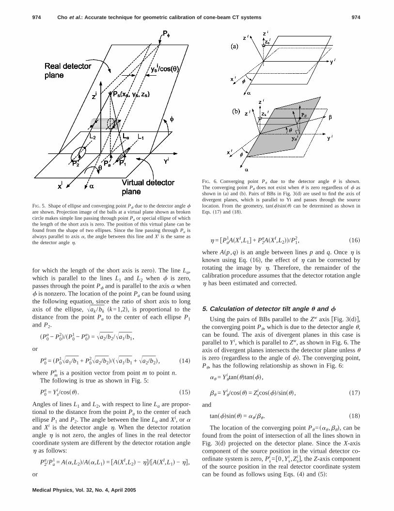
974 Cho et al. : Accurate technique for geometric calibration of cone-beam CT systems 974
for which the length of the short axis is zerod. The lineLa,which is parallel to the linesL1 and L2 when f is zero,passes through the pointPf and is parallel to the axisa whenf is nonzero. The location of the pointPa can be found usinthe following equation, since the ratio of short axis to loaxis of the ellipse,Îak/bk sk=1,2d, is proportional to thdistance from the pointPa to the center of each ellipseP1
andP2.
sP0a − P0
2d/sP01 − P0
ad = Îa2/b2/Îa1/b1,
or
P0a = sP0
1Îa1/b1 + P02Îa2/b2d/sÎa1/b1 + Îa2/b2d, s14d
wherePmn is a position vector from pointm to point n.
The following is true as shown in Fig. 5:
P0a = Ys
i /cossud. s15d
Angles of linesL1 andL2, with respect to lineLa are proportional to the distance from the pointPa to the center of eacellipseP1 andP2. The angle between the lineLa andXi, or aand Xi is the detector angleh. When the detector rotatioangleh is not zero, the angles of lines in the real detecoordinate system are different by the detector rotation ah as follows:
P2a/Pa
1 = Asa,L2d/Asa,L1d = fAsXI,L2d − hg/fAsXI,L1d − hg,
FIG. 5. Shape of ellipse and converging pointPf due to the detector anglefare shown. Projection image of the balls at a virtual plane shown as bcircle makes simple line passing through pointPa or special ellipse of whicthe length of the short axis is zero. The position of this virtual plane cafound from the shape of two ellipses. Since the line passing throughPa isalways parallel to axisa, the angle between this line andXi is the same athe detector angleh.
or
Medical Physics, Vol. 32, No. 4, April 2005
e
h = fPa1AsXI,L1g + P2
aAsXI,L2dd/P12, s16d
whereAsp,qd is an angle between linesp andq. Onceh isknown using Eq.s16d, the effect ofh can be corrected brotating the image byh. Therefore, the remainder of tcalibration procedure assumes that the detector rotationh has been estimated and corrected.
5. Calculation of detector tilt angle u and f
Using the pairs of BBs parallel to theZw axis fFig. 3sddg,the converging pointPu, which is due to the detector angleu,can be found. The axis of divergent planes in this casparallel toYi, which is parallel toZw, as shown in Fig. 6. Thaxis of divergent planes intersects the detector plane unuis zerosregardless to the angle offd. The converging poinPu, has the following relationship as shown in Fig. 6:
au = Yui tansudtansfd,
bu = Yui /cossud = Zs
i cossfd/sinsud, s17d
and
tansfdsinsud = au/bu. s18d
The location of the converging pointPu=sau ,bud, can befound from the point of intersection of all the lines shownFig. 3sdd projected on the detector plane. Since theX-axiscomponent of the source position in the virtual detectorordinate system is zero,Ps
i =f0,Ysi ,Zs
i g, theZ-axis componenof the source position in the real detector coordinate sy
n
FIG. 6. Converging pointPu due to the detector angleu is shownThe converging pointPu does not exist whenu is zero regardless off asshown insad and sbd. Pairs of BBs in Fig. 3sdd are used to find the axisdivergent planes, which is parallel to Yi and passes through the slocation. From the geometry, tansfdsinsud can be determined as shownEqs.s17d and s18d.
can be found as follows using Eqs.s4d and s5d:

xntof
ec-e
hod
g
--
Fig.
all, re-
n be
lineing
l-n
ecteptf
two
ing
ce
-
975 Cho et al. : Accurate technique for geometric calibration of cone-beam CT systems 975
ZsI = Zs
i cossudcossfd + Ysi sinsud
= sinsudcossudfbu + Ysi /cossudg. s19d
From the ellipse model in Eqs.s9d ands10d, f is propor-tional to Zs
I , whenab−c2 is greater than zerosSee Appendifor the proofd. Sincebu is known from the converging poiof Pu andYs
i /cossud is known from the converging pointPf , Zs
I is simply a function of the detector angle ofu, and isproportional tou when is less than 45°. Thereforeu is pro-portional tof in ellipse model as shown in Fig. 7. Interstion of two lines, one from Eq.s18d and the other from thEqs. s9d, s10d, and s19d is the solution off and u. Thissolution can be found using a nonlinear root finding metThere is a unique solution when the angle ofu is less than45° as shown in Eq.s19d.
6. Calculation of source position „XsYsZs…I
Oncef and u are known,Ysi and Zs
i can be found usinEqs. s15d and s17d, respectively. Whenu is infinitesimallysmall se.g., less than 0.001 degd, however, Eq.s17d is not
FIG. 7. Solution ofu andf can be determined from the intersection ofcurves; one from Eq.s18d and the other from the ellipse model in Eqs.s9d,s10d, and s19d. The solution can be found using the nonlinear root findmethod. There is a unique solution when the angle ofu is less than 45°.
FIG. 8. Distance between two ellipses,L1 andL2 can be related with sourto detector distanceZs
i , and iso-center to detector distanceZdi using the
triangulation of the projection, when detector angleh and u are compen
sated. See the calibration section for details.Medical Physics, Vol. 32, No. 4, April 2005
.
stable enough to estimateZsi . Whenu is this small, the fol
lowing methods are used to estimateZsi . The distance be
tween two ellipses along theYi axis, L1 and L2 have thefollowing relations due to the triangulation as shown in8:
L1/Zsi = l/sZs
i − Zdi + radd, s20d
L2/Zsi = l/sZs
i − Zdi − radd, s21d
where, rad andl are the radius of the circular pattern of bbearing and distance between two circular trajectoriesspectively. Combining two equations to calculateZs
i gives
Zsi = s2 radL1L2d/flsL2 − L1dg. s22d
Having known three detector anglessh , f, andud and thesource position in the virtual detector coordinate systemsYs
i
andZsi d, the source position in the real detector system ca
calculated straightforwardly using Eqs.s4d and s5d as fol-lows. sNote: Xs
i is zero by definitiond.
PsI = Ri
IPsi .
7. Calculation of detector position „Yd ,Zd…i
One of the detector position vector,Zdi , can be found from
Eqs.s20d and s21d.
Zdi = Zs
i sL1 − ld/L1 + r . s23d
Since the origin of the world coordinate system is on theconnecting the piercing point and the source, the followrelationship is true:
Ydi = Ys
i /Zsi Zd
i . s24d
8. Gantry angle determination
The nominal gantry anglet can be calculated by the folowing procedure. Equationss6ad and s6bd can be rewritteas follows:
sXsI − Xd/sXs
I − XId = sYsI − Yd/sYs
I − YId s25d
or
YsI − YI = sXs
I − XIdsYsI − Yd/sXs
I − Xd = psXsI − XId, s26d
wherep=sYsI −Yd / sXs
I −Xd can be calculated for each objpoint PI =fXI ,YI ,ZIgT. Since all the other parameters excnominal gantry angle are known,XI andZI are functions onominal gantry anglet only. Rearranging Eq.s26d gives
fb1b2gfSt CtgT = A s27d
and
b1 = spr1 − r4dxw + spr3 − r6dyw,
w w
b2 = s− pr3 + r6dx + spr1 − r4dy ,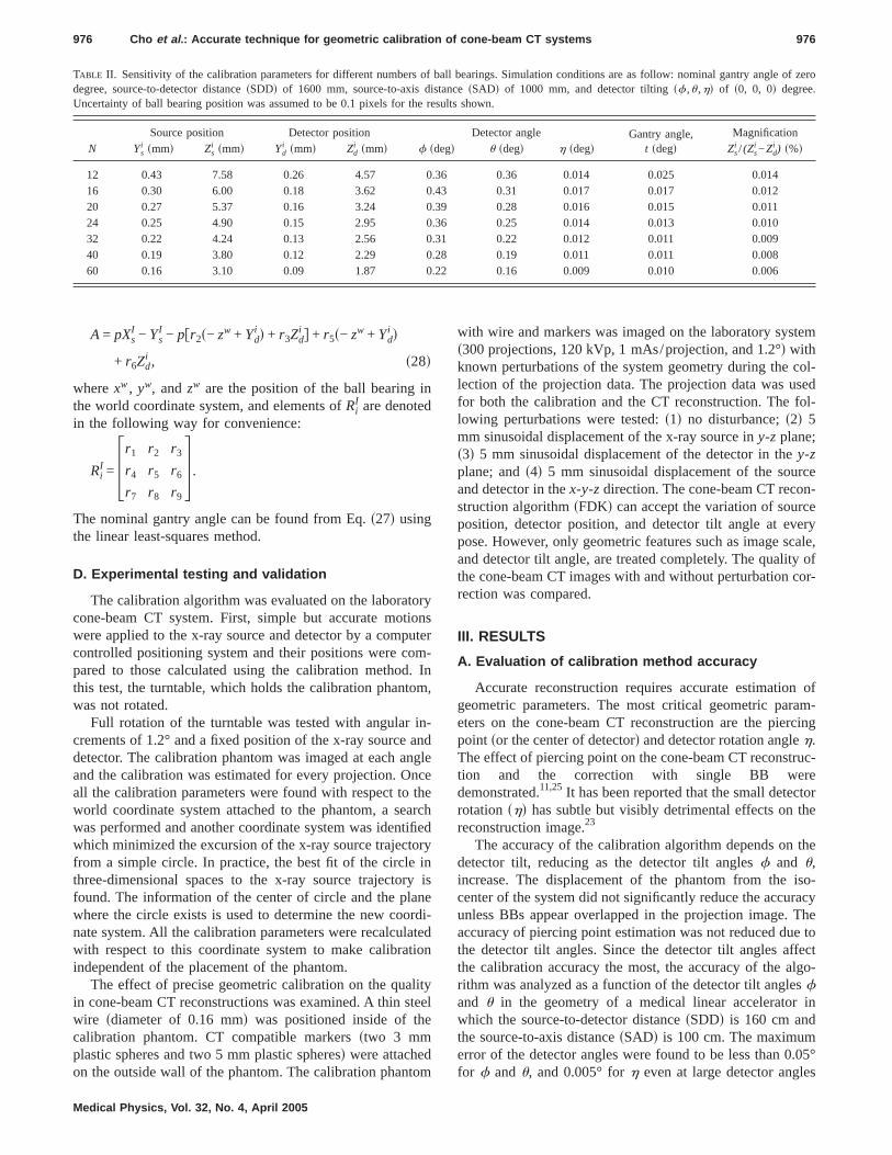
ind
torytionputeom-d. Intom
in-and
angncethe
earctifietory
inry ianeordilatetion
litysteee
d
stem
col-usedfol-
rcen-
rceveryscale,ty ofcor-
n ofram-rcing
truc-rectorthe
the
iso-racy
. Theue toffectalgo-esr in
0.05°
le of z.
976 Cho et al. : Accurate technique for geometric calibration of cone-beam CT systems 976
A = pXsI − Ys
I − pfr2s− zw + Ydi d + r3Zd
i g + r5s− zw + Ydi d
+ r6Zdi , s28d
wherexw, yw, andzw are the position of the ball bearingthe world coordinate system, and elements ofRi
I are denotein the following way for convenience:
RiI = 3r1 r2 r3
r4 r5 r6
r7 r8 r94 .
The nominal gantry angle can be found from Eq.s27d usingthe linear least-squares method.
D. Experimental testing and validation
The calibration algorithm was evaluated on the laboracone-beam CT system. First, simple but accurate mowere applied to the x-ray source and detector by a comcontrolled positioning system and their positions were cpared to those calculated using the calibration methothis test, the turntable, which holds the calibration phanwas not rotated.
Full rotation of the turntable was tested with angularcrements of 1.2° and a fixed position of the x-ray sourcedetector. The calibration phantom was imaged at eachand the calibration was estimated for every projection. Oall the calibration parameters were found with respect toworld coordinate system attached to the phantom, a swas performed and another coordinate system was idenwhich minimized the excursion of the x-ray source trajecfrom a simple circle. In practice, the best fit of the circlethree-dimensional spaces to the x-ray source trajectofound. The information of the center of circle and the plwhere the circle exists is used to determine the new conate system. All the calibration parameters were recalcuwith respect to this coordinate system to make calibraindependent of the placement of the phantom.
The effect of precise geometric calibration on the quain cone-beam CT reconstructions was examined. A thinwire sdiameter of 0.16 mmd was positioned inside of thcalibration phantom. CT compatible markersstwo 3 mmplastic spheres and two 5 mm plastic spheresd were attache
TABLE II. Sensitivity of the calibration parameters for different numberdegree, source-to-detector distancesSDDd of 1600 mm, source-to-axisUncertainty of ball bearing position was assumed to be 0.1 pixels for
N
Source position Detector positionYs
i smmd Zsi smmd Yd
i smmd Zdi smmd f s
12 0.43 7.58 0.26 4.5716 0.30 6.00 0.18 3.6220 0.27 5.37 0.16 3.2424 0.25 4.90 0.15 2.9532 0.22 4.24 0.13 2.5640 0.19 3.80 0.12 2.2960 0.16 3.10 0.09 1.87
on the outside wall of the phantom. The calibration phantom
Medical Physics, Vol. 32, No. 4, April 2005
sr
,
le
hd
s
-d
l
with wire and markers was imaged on the laboratory sys300 projections, 120 kVp, 1 mAs/projection, and 1.2°d withknown perturbations of the system geometry during thelection of the projection data. The projection data wasfor both the calibration and the CT reconstruction. Thelowing perturbations were tested:s1d no disturbance;s2d 5mm sinusoidal displacement of the x-ray source iny-z plane;s3d 5 mm sinusoidal displacement of the detector in they-zplane; ands4d 5 mm sinusoidal displacement of the souand detector in thex-y-z direction. The cone-beam CT recostruction algorithmsFDKd can accept the variation of souposition, detector position, and detector tilt angle at epose. However, only geometric features such as imageand detector tilt angle, are treated completely. The qualithe cone-beam CT images with and without perturbationrection was compared.
III. RESULTS
A. Evaluation of calibration method accuracy
Accurate reconstruction requires accurate estimatiogeometric parameters. The most critical geometric paeters on the cone-beam CT reconstruction are the piepoint sor the center of detectord and detector rotation angleh.The effect of piercing point on the cone-beam CT reconstion and the correction with single BB wedemonstrated.11,25It has been reported that the small deterotation shd has subtle but visibly detrimental effects onreconstruction image.23
The accuracy of the calibration algorithm depends ondetector tilt, reducing as the detector tilt anglesf and u,increase. The displacement of the phantom from thecenter of the system did not significantly reduce the accuunless BBs appear overlapped in the projection imageaccuracy of piercing point estimation was not reduced dthe detector tilt angles. Since the detector tilt angles athe calibration accuracy the most, the accuracy of therithm was analyzed as a function of the detector tilt anglfand u in the geometry of a medical linear acceleratowhich the source-to-detector distancesSDDd is 160 cm andthe source-to-axis distancesSADd is 100 cm. The maximumerror of the detector angles were found to be less than
all bearings. Simulation conditions are as follow: nominal gantry angeroncesSADd of 1000 mm, and detector tiltingsf ,u ,hd of s0, 0, 0d degreeesults shown.
Detector angle Gantry angle,t sdegd
Magnificationu sdegd h sdegd Zs
i / (Zsi −Zd
i ) s%d
0.36 0.014 0.025 0.0140.31 0.017 0.017 0.0120.28 0.016 0.015 0.0110.25 0.014 0.013 0.0100.22 0.012 0.011 0.0090.19 0.011 0.011 0.0080.16 0.009 0.010 0.006
s of bdistathe r
degd
0.360.430.390.360.310.280.22
for f andu, and 0.005° forh even at large detector angles

gle
tionor
to. As
rithmtionsy ofcon
ro-actlrthto
t isitiv-se oare
ne a
eura-of afol-y of
theccel
ntyto
sts othisBBumthewerr ptposi
24of
ity isty ofglesr ofTheat
tectord us-
dis-osi-
ed bynal,
ciesin
matedc--rep-
f they in-of thehat thety ofaoristo
977 Cho et al. : Accurate technique for geometric calibration of cone-beam CT systems 977
sf=u= ±40°d. In the practical range of the detector tilt anf andu! ±5°, the error of the detector tilt anglesf , u , h,and magnification factor were negligible. The magnificafactor was determined as the ratio of SDD to SADZs
i / (Zsi −Zd
i ). Error in the magnification factor was foundbe less than 0.05% at a large detector tilt angle of ±40°discussed in the next section, the inaccuracy of the algois less than the uncertainties arising from the imperfecin phantom construction and BB detection. The sensitivitthe algorithm to these uncertainties should be taken intosideration.
B. Sensitivity analysis
The calibration method is an analytic method, which pvides exact results when the positions of the BBs are exknown and the number of BBs is larger than 12. It is woexploring the sensitivity of the calibration algorithm duethe uncertainty of the ball bearing position. Although ipossible to derive direct analytical solutions for the sensity analysis, a numerical method is often preferred becauits simplicity. Thus, the resulting estimations in this studyapproximate. The sensitivityDX in an arbitrary calibratioparameterX can be estimated in a root mean square sens
DX = dFoi=1
S ]X
]UiD2
+ S ]X
]ViD2G0.5
, s29d
whered is the uncertainty of the ball bearing location, andUi
andVi are the location of thei-th BB. The uncertainty of thball bearing location may include manufacturing inacccies and uncertainty in the identification of the centerBB. Instead of calculating direct partial derivatives, thelowing equation was used to approximate the sensitivitthe calibration algorithm:
DX = dHoi=1
FSXsUi + dUid − XsUi − dUid2dUi
D2
+ SXsVi + dVid − XsVi − dVid2dVi
D2GJ0.5
. s30d
.Table II summarizes the effect of number of BBs on
sensitivity for a system as exists on the medical linear aerator sSDD=160 cm and SAD=100 cmd. The sensitivityanalysis was based on the assumption that the uncertaiball bearing positiond was 0.1 pixels. This correspondsthe manufacturing inaccuracy of 25µm or error of 0.1 pixelin the image processing. Since one ball bearing consismore than 200 pixels in the image in this configuration,would be a reasonable assumption. Larger numbers ofreduced the uncertainty as shown in Table II. When the nber of BBs was doubled from 16 to 32, the uncertainty ofsource position, detector position, and detector anglesreduced by about 30% on average. Source and detectositions in the direction of beamsZs
i and Zdi were the mos
sensitive parameters to the uncertainty of ball bearingi i
tion. Although the uncertainty ofZs andZd were large aboutMedical Physics, Vol. 32, No. 4, April 2005
-
y
f
s.
-
of
f
s-
eo-
-
0.5% s4.9 mm at SAD of 1000 mm for the phantom withBBsd, the uncertainty of the magnification factor, the ratioSDD sZs
i d to SAD sZsi −Zd
i d, was relatively smalls0.01 %d.Therefore, the impact on the reconstructed image qualexpected to be negligible. Figure 9 shows the sensitivithe calibration parameters as a function of detector tilt anf andu. The sensitivity of the algorithm appears an ordemagnitude larger than the accuracy of the algorithm.sensitivity of the algorithm, however, is very small evenvery large detector tilt angles as shown in Fig. 9.
C. Experimental testing of geometry
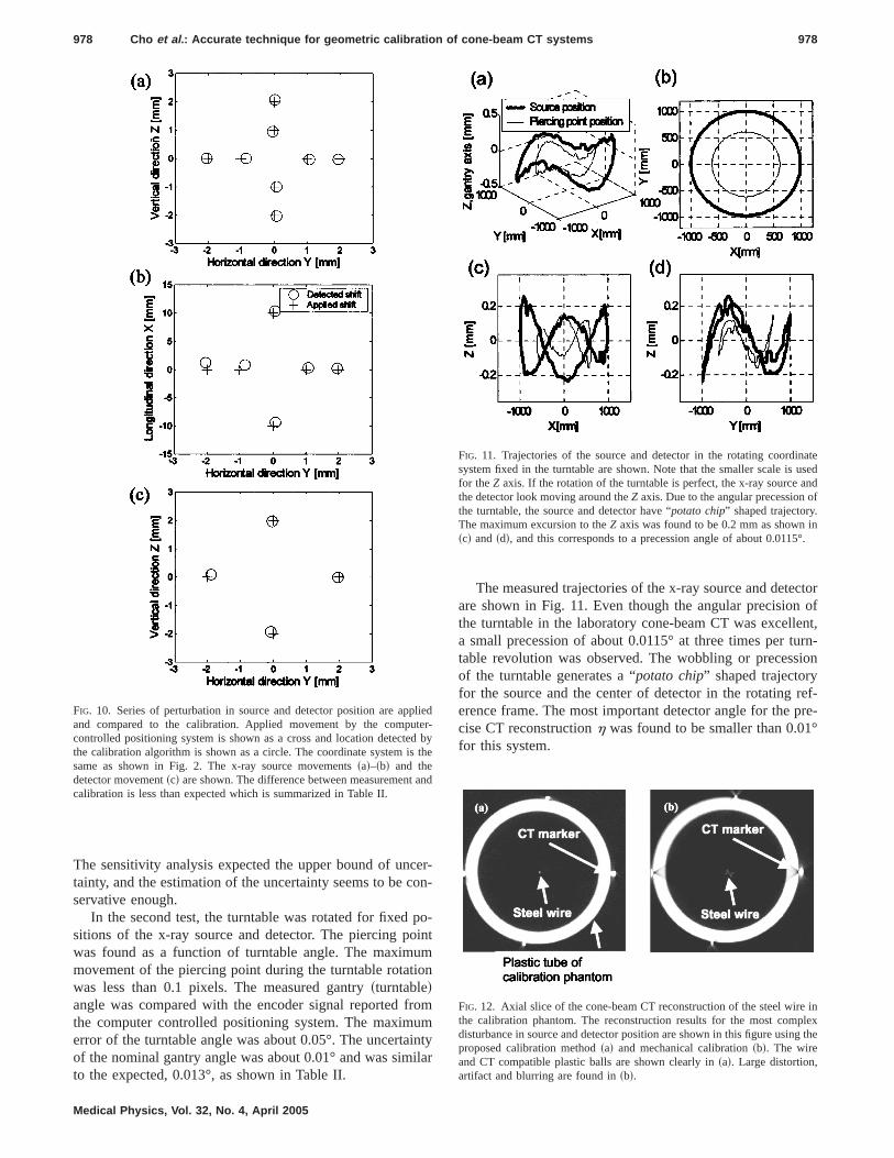
A series of accurate displacements in source and deposition were applied and compared to those calculateing the calibration method. Figures 10sad and 10sbd show theapplied and measured result when the x-ray source isplaced. Applied movement by the computer-controlled ptioning system is shown as a cross and location detectthe calibration algorithm is shown as a circle. Longitudihorizontal, and vertical directions correspond toX, Y, andZof the world coordinate system, respectively. Discrepanin the x-ray source positions were found to be 0.08 mmthe direction normal to the beamsY- and Z-axis directiondand 0.8 mm in the beam directionsX-axis directiond. Thesemeasured discrepancies were less than those estithrough the sensitivity analysiss0.25 and 4.9 mm, respetively as shown in Table IId. Figure 10scd shows the calibration result when the detector position is moved—the disc
FIG. 9. Sensitivity of the calibration algorithm due to the uncertainty oball bearing position. The uncertainty of the ball bearing location maclude manufacturing inaccuracies and uncertainty in the identificationcenter of a BB. The sensitivity analysis was based on the assumption tuncertainty of the ball bearing position was 0.1 pixels. The sensitividetector anglessad–scd and the magnification factorsdd are shown asfunction of detector tilt anglesf andu, in typical medical linear acceleratin which source-to-detector distancesSDDd of 160 cm and source-to-axdistancesSADd of 100 cm. The magnification factor is the ratio of SDDSAD.
ancy in the detector position was found to be about 0.06 mm.
cercon
pooinum
tion
fromum
aintyila
tectorn ofllent,turn-sionyref-pre-1°
pplieuter-ted bis the
t and
inates usedandof
.in
5°.
ire inplex
ng the
,
978 Cho et al. : Accurate technique for geometric calibration of cone-beam CT systems 978
The sensitivity analysis expected the upper bound of untainty, and the estimation of the uncertainty seems to beservative enough.
In the second test, the turntable was rotated for fixedsitions of the x-ray source and detector. The piercing pwas found as a function of turntable angle. The maximmovement of the piercing point during the turntable rotawas less than 0.1 pixels. The measured gantrysturntabledangle was compared with the encoder signal reportedthe computer controlled positioning system. The maximerror of the turntable angle was about 0.05°. The uncertof the nominal gantry angle was about 0.01° and was sim
FIG. 10. Series of perturbation in source and detector position are aand compared to the calibration. Applied movement by the compcontrolled positioning system is shown as a cross and location detecthe calibration algorithm is shown as a circle. The coordinate systemsame as shown in Fig. 2. The x-ray source movementssad–sbd and thedetector movementscd are shown. The difference between measuremencalibration is less than expected which is summarized in Table II.
to the expected, 0.013°, as shown in Table II.
Medical Physics, Vol. 32, No. 4, April 2005
--
-t
r
The measured trajectories of the x-ray source and deare shown in Fig. 11. Even though the angular precisiothe turntable in the laboratory cone-beam CT was excea small precession of about 0.0115° at three times pertable revolution was observed. The wobbling or precesof the turntable generates a “potato chip” shaped trajectorfor the source and the center of detector in the rotatingerence frame. The most important detector angle for thecise CT reconstructionh was found to be smaller than 0.0for this system.
d
y
FIG. 11. Trajectories of the source and detector in the rotating coordsystem fixed in the turntable are shown. Note that the smaller scale ifor theZ axis. If the rotation of the turntable is perfect, the x-ray sourcethe detector look moving around theZ axis. Due to the angular precessionthe turntable, the source and detector have “potato chip” shaped trajectoryThe maximum excursion to theZ axis was found to be 0.2 mm as shownscd and sdd, and this corresponds to a precession angle of about 0.011
FIG. 12. Axial slice of the cone-beam CT reconstruction of the steel wthe calibration phantom. The reconstruction results for the most comdisturbance in source and detector position are shown in this figure usiproposed calibration methodsad and mechanical calibrationsbd. The wireand CT compatible plastic balls are shown clearly insad. Large distortion
artifact and blurring are found insbd.
ality
heim-
e.
orteired
of aumwasrenon-
ss ofthe
nt in
lera-was
thanhenr indical
ion. Thiscali-ap-
com-
iselybe.gThe
d haseterand
om aand
ionCBCing
ehery-
ith--.
979 Cho et al. : Accurate technique for geometric calibration of cone-beam CT systems 979
D. Influence of calibration on image quality
The effect of accurate geometric calibration on the quof reconstructions was examined using a thin steel wiresdi-ameter of 0.16 mmd positioned within the BB phantom at ttime of calibration. Figure 12 shows the cone-beam CTages using the proposed calibration algorithmsad and themechanical calibrationsbd for the most complex disturbancThe wire and plastic balls are shown clearly insad, but largedistortion, artifact, and blurring are found insbd. Figure 13shows surface plots of the attenuation coefficients repby the cone-beam CT method for a thin steel wire acquwith sad the circular motion with the calibration method,sbdcomplex disturbancefsee 4th condition in Sec. II Dg with thecalibration,scd circular motion without calibration, and,sddcomplex disturbancefsee 4th condition in Sec. II Dg withoutcalibration. The intensity of the cone-beam CT imagethin wire was symmetric and the full width at half maximsFWHMd was 0.78 mm. Improvement in the peak signal53% in the steel wire on average across the four diffecases as shown in Table III. Signal from the wire was c
TABLE III. Influence of calibration on imaging quality in the reconstructof a steel wire. The dataset was acquired on the laboratory benchsystem with mechanical determination of the imaging geometry assumcircular trajectory.
FWHM smmd Signal sarbitraryd
Without calibration algorithm 0.99 mm 0.27With calibration algorithm 0.78 mm 0.41
Improvement 28% 53%
Medical Physics, Vol. 32, No. 4, April 2005
d
t
sistent when the calibration method was used regardlethe disturbance applied. Artifact and distortion aroundmarker was also reduced. On average, improvemeFWHM of the steel wire was 28%.
Similar tests were performed on a medical linear accetor. In these investigations, an error in geometric scaleidentified. The diameter of the phantom was 5% largermanufacturing specifications and agreed within 0.2% wthe full calibration method was employed. This large errothe dimensional accuracy in cone-beam CT on the melinear accelerator was due to the use of a nominal SDDs160cm versus 153 cmd in the previous calibration scheme.
IV. DISCUSSION AND CONCLUSIONS
A new method for the geometric calibration of projectimaging systems has been developed and demonstratedmethod is robust, easy to implement, and general. Thebration algorithm uses a linear parameter-estimationproach for fast and accurate computation. It produces aplete solutionsall the calibration parameters are foundd usinga calibration phantom consisting of 24 steel BBs preclocated in two circular patterns in a cylindrical acrylic tuAlthough calculation off andu uses a nonlinear root findinmethod, a unique, convergent solution is guaranteed.method has been employed in realistic geometries andemonstrated accuracy and precision to permit submillimcharacterization of the relative positions of the sourcedetector components. This determination is extracted frsingle projection. The image processing, BB detection,
Ta
FIG. 13. Surface plots of axial slicimages of a thin steel wire, where tsignal of the image has an arbitraunit. Circular motion with the proposed calibration methodsad, complexmotion of source and detector wcalibration sbd, circular motion without calibrationscd, and complex motion without calibrationsdd are shown
analysis is performed in a few seconds with the current, non-

tionsec.cali-ion”im-rmithetemnot
,na-fea-dd biza-re-
ed tthe
c-he
ecto
de are-
es.be
trictotthe. Inon oballnsarionacts
temakeingsidme
f theconu-mizaeantrixap-ery
isticas
wee
ion ofeenen ma-etter. Sys-edtheirre as-n of
o there-con-
hreepaper0 degtheuch
l testivityf the
tra-s asAbil-el ofmul-
l as-that
r ordol-se atusedajec-cone-greed
f anyce.ulti-duc-ustper-two
ni-te re-oftedduc-that.
o ao en-e-
terialoach
980 Cho et al. : Accurate technique for geometric calibration of cone-beam CT systems 980
optimized version. It is feasible to have these determinacompleted in real time at frame rates of 15–30 frames/
It may be of some value to the reader to relate thisbration approach to the literature of “pose determinatfound in the field of visualization, graphics, and opticalaging. The algorithm can be referred to as a “pose detenation” algorithm, the purpose of which is to determinegeometric and optical characteristics of an imaging sysIn this context, however, the extracted information refersto the subjectsphantomd, but rather, to the “camera”si.e.,source and detectord. Visible calibration objectssin this casethe calibration phantomd were used for the pose determition. The calibration object consists of many geometrictures, such as points and lines,26 which are easily identifiein the image, and the geometry of the features shoulknown for the calibration. Even though nonlinear optimtion techniques27 have been applied, implementation hasmained a problem.
The method described in this paper can be comparother image-based calibration approaches. Followingwork of Rougee22 and others,29 there exists a linear projetion matrix relating 3D voxels onto 2D projection image. Tprojection matrix is a function of intrinsic parameterssthecenter of image and distance between source and detdand extrinsic parameterssrotation and translationd. The mainuse of the imaging geometry characterization is to provicorrect 3D to 2D mapping between the 3D voxels to beconstructed and the 2D pixels on the radiographic imag20
In this context, the projection matrix does not have todecomposed for the identification of the individual geomeparameters.21 The projection matrix can be simplified intwo parametersscenter of imaging systemd by assuming thathe imaging system is rigid and the only nonideality issmall translational motion parallel to the axis of rotationthis approach, a map of the center of detector as a functithe gantry angle found from the x-ray image of a singlebearing at the isocenter of the system is used to compefor these nonideal motions of the C-arm18 and medical lineaaccelerator.1,11,25 Images reconstructed without correctsuffer from loss of detail, misregistration, and streak artifcompared to those with this simple correction.1 However,this approach would become less appropriate for systhat exhibit large deviations from the ideal trajectory. To tinto account of all the possible nonidealities of the imagsystem geometry, the full projection matrix has been conered in the calibration process. Since the number of georic parameters is less than the number of freedom oprojection matrix, unstable results are expected for unstrained approach.22 To overcome the difficulties, various nmerical constraints have been developed such as optition of the parameters to minimize the reprojection mquadratic error, and decomposition of the projection mainto intrinsic and extrinsic geometric parameter. In theproach of nonlinear optimization, it was reported to be vsensitive to the initial conditions and may lead to unrealvalues.28 In the linear decomposition approach, such ansumption that intrinsic parameters are not changed bet
two consecutive frames was used for reliable estimation oMedical Physics, Vol. 32, No. 4, April 2005
s
-
.
e
o
r
f
te
s
-t-
-
-
-n
the geometric parameters. Even though the decompositthe projection matrix may not be impossible, it has bknown to be difficult and unstable.18 Knowing the completgeometric parameters has advantages over the projectiotrix method; one can characterize the imaging system band diagnosis the system performance numerous waystematic and analytic linear methods23,24have been developfor the geometric parameters estimation. However,methods are not fully general, as some parameters asumed to be zero or constant and known. The precisiothe proposed algorithm was proved to be comparable tprevious reports23,22 at small detector angles. While the pcision of the previous studies were evaluated under suchditions that one or two detector angles were zero, or all tangles were close to zero, the proposed method in thiswas evaluated at the extended detector angles of up to 4in all directions. The uncertainty analysis showed thatprecision of the proposed algorithm does not degrade mat such a large range of detector angles. An experimentaeven outperformed the expectation from the sensitanalysis, which shows the upper bound of uncertainty oalgorithm.
The method can be applied to characterize complexjectories of the source and detector in multiview problemdemonstrated here in the application to cone-beam CT.ity to characterize these multiview systems to a high levaccuracy and precision creates the opportunity to adapttiview volumetric imaging systems to various mechanicasemblies that may not have mechanical characteristicsconform to conventional trajectories such as the circulaspiral motion employed in conventional CT. The methoogy developed here permits characterization of the pomany points over the course of this motion and can bein retrospect provided the device has a reproducible trtory. This retrospective approach has been employed inbeam CT applications highlighted in this paper. The deof reproducibility will limit the application of the methojust as the mechanical imprecision and inaccuracies opurpose-built mechanical system would limit performan
The methodology also permits the employment of mview approaches in systems that do not satisfy the reproibility requirement. In such an approach, the imaging mbe performed in the context of the phantom and therebymit prospective pose determination. This approach hasimportant features:sid significant relaxation of the mechacal precision and accuracy necessary to achieve accuraconstructions; andsii d dynamic, feedback-based collectionthe projection data with the possibility of operator-direcpose selection. The impact of the first feature is in the retion of the cost of precise imaging systems, such asrequired in high-resolutions10 µmd small sample imagingThe option for adaptation of multiview approaches tbroader spectrum of existing mechanical systems is alshanced. For example, the utilization of highly flexible mchanical systems, such as, multiaxis robotic arms or mahandling/conveyor systems would be feasible. This appr
fallows the precision and accuracy of the image to be decou-
sys
d ofan
. Therconurac
retom
ctions ofrferndtheesetemex-
tec-erald tos ngeoBsar
mestemose. Thboraservs-
theoul
l foro inip
andpeeresiblctedd acs togh-conlo-for
f thf acn o
-he
mis-
thethe
x-rayof a
singe inhere
oni-m’s
applyin aaln.
gh-us-lar
algo-for
d thatith aeamf thestems
theali-anyrces
Thesethee sys-MVatorVbe-
ylego-e inhis
as-
981 Cho et al. : Accurate technique for geometric calibration of cone-beam CT systems 981
pled from the precision and accuracy of the mechanicaltem used for positioning of the source and detector.
The phantom employed in this investigation consiste24 BBs on two,100 mm diameter circles. The method cbe readily adapted to a range of phantom configurationsnumber of BBs is unlimited with a minimum of eight pring. The number of BBs employed is selected throughsideration of the desired robustness, precision, and accof the overall system. An increased number of BBs canduce the influence of mechanical imprecision in the phanconstruction; however, systematic errors in the construof the phantom would remain a factor. Larger numberBBs can be advantageous when imaging conditions intewith BB detection within a projection. The diameter aseparation of the circular BB patterns will also influencealgorithm’s performance. The selection of values for thparameters is a compromise between the imaging sysfield of view and the desired geometric performance. Ancessively small ring diameter may interfere with BB detion, depending on the size of the BBs employed. In genthe spatial extent of the phantom should be maximizeproduce the greatest geometric performance. This doepreclude the use of very small phantoms to determinemetric information in a localized fashion provided the Bcan be identified. Often the detectors of CBCT systemsshifted laterally to increase the CT scan field of view. If sooverlapping areas are allowed in the detector shift syand the BBs can be identified in both images, the propmethod can be used for these detector-offset situationsaverage phantom error from the measurements in the latory bench seems to be underestimated due to the contive uncertainty analysis in this paperssince errors are asumed to be accumulated without cancel outd. To study theeffect of systematic errors in the calibration phantom onuncertainty accurately, better measure of uncertainty shbe employed.
The accurate determination of pose is not only usefuimaging, but also for relating the image-based results tterventional devices.29 Of specific interest is the relationshof the cone-beam CT images to the megavoltagesMV d treat-ment beam used for radiation therapy. The MV sourcelarge-area flat-panel detector used for portal imaging arefectly suited to the calibration approach developed hThrough the use of a single phantom placement, it is posto relate the trajectory of the MV source to the reconstrucone-beam CT sets with a high degree of precision ancuracy. The phantom requires modification of the BBpermit visualization at MV energies; for example, hidensity material such as tungsten improves the imagetrast. In addition to determining the source position, thecation of beam defining devices can also be assessedgiven pose. In general, all the mechanical aspects otreatment device can be characterized to a high level ocuracy and precision. This approach permits quantificatiopatient couch motionsdisplacements and rotationsd, collima-tor rotation, as well as, collimatorsmultileaf, leaf bank, independent jawsd position over a range of gantry angles. T
method offers the opportunity to provide quantitative resultsMedical Physics, Vol. 32, No. 4, April 2005
-
e
-y
-
e
’s
,
ot-
e
de-
a-
d
-
r-.e
-
-
ae-f
for these mechanical systems in the processes of comsioning, on-going quality assurance, and recalibration.
In addition to characterizing the location of objects inprojected field of view, the methodology can also look attemporal aspects of these systems. Instabilities in thesource position can also be quantified over the coursebeam segment by collecting multiple frames or movies uthe portal imaging device. This capacity is of great valuthe context of intensity modulated radiation therapy wradiation therapy beam segments can contain very few mtor units, resulting in beam completion before the systeservos are able to stabilize. The same approach wouldto other temporal instabilities, such as focal spot wobbleconventional x-ray tube,30 vibrational modes of a mechanicassembly, and, shifts induced by focal spot size selectio
An accurate geometric calibration is important for hiprecision image-guided radiation therapy. A new methoding a calibration phantom, which consists of two circupatterns of BBs, has been developed. The calibrationrithm employs a linear parameter-estimation approachfast and accurate computation. It has been demonstratethe method is robust and produces a complete solution whigh level of accuracy. The method can improve cone-bCT image quality, characterize the mechanical motion osystem, and cross-calibrate imaging and treatment syfor high-precision image guided radiation therapy. Sinceproposed method is not only limited to the geometric cbration of CBCT systems but also can be used for mother systems, which consist of one or more point souand area detectors, various applications are possible.include the calibration of a MV treatment system forquality assurance, acceptance test, and diagnosis of thtem sfocal spot movement during the beam delivery,source trajectory versus gantry angle, the axis of collimrotation, and couch motiond, cross calibration between kimaging and MV treatment system, and cross calibrationtween multiple imaging systems.
ACKNOWLEDGMENTS
The authors would like to acknowledge Dr. R. Clackdoand Dr. F. Noo for providing their FDK reconstruction alrithm, which formed the basis of the reconstruction codthis investigation and for providing invaluable advice. Twork was supported in part by NIH/NIBIBsR01EB002470dand Elekta Oncology Systems.
APPENDIX
1. Lines parallel to virtual detector plane from theellipse model
For the sake of simplification, the center of ellipse issumed to bes0,0d as follows:
aU2 + bV2 + 2cUV= 1 sA1d
or

ing
,Eq.ints
m-con-
ially
asng abe
nts
nt
by
982 Cho et al. : Accurate technique for geometric calibration of cone-beam CT systems 982
V2 + S2c
bUDV + Sa
bU2 −
1
bD = 0. sA2d
When the discriminant ofV equals to zero, the correspondU equals either maximum or minimum value as follows:
S c
bUD2
− Sa
bU2 −
1
bD = 0 sA3d
or
U = ±Î b
ab− c2 sA4d
and
V = −c
bU. sA5d
SinceU has two real roots in Eq.sA4d, andb is real positiveab−c2 is greater than zero. As shown in Fig. 14 andsA5d, the slope of the line passing through the two po
FIG. 14. Line parallel to the virtual detector plane.
FIG. 15. Extension to lar
Medical Physics, Vol. 32, No. 4, April 2005
found in Eqs.sA4d andsA5d is determined by ellipse paraeters. Two lines from each ellipse are used to find theverging point,Pf.
2. Extension to large detector angles
SincePu has an angle of tanf3sinu with the axis ofV,Eqs.sA4d andsA5d are not accurate in general and especfor a very large detector angle,f andu. A line, which con-nects the outmost position of the two ellipses showndashed line in Fig. 15, should be used instead of usiparallel line to theV axis. An equation of the line canwritten using two parameters,A andB as follows:
U = A 3 V + B. sA6d
The slope of the lineA can be approximated using two poifrom each ellipse using Eqs.sA4d and sA5d.
A < sU1 − U2d/sV1 − V2d = sU1 − U2d/sU1c1/b1 − U2c2/b2d.
sA7d
From Eqs.sA1d andsA6d, the condition of zero descriminaof each ellipsesk=1,2d can be found as follows:
sck2 − akbkdBk
2 + saka2 + bk + 2ckAd = 0
or
Bk = ±Îbk + akA2 + 2ckA
akbk − ck2 , sA8d
whereB has one trivial solution and it can be found easilycomparing the sign withsU1+U2d /2.
ge detector tilt angles.

lat-iation
y.
ging
om-
orBiol.
ane-
n-ients
ge.
. A.and
raphyed.
-r foriol.,
-ed.
on
i.
nrota-
eldicalures
aSPIE
phicon of
nsferplat-dical
cging
CAI
libra-om-
nbeam
ys-
erize
hine
ctor
ton,hys.
etricedicalm-
Re-.
983 Cho et al. : Accurate technique for geometric calibration of cone-beam CT systems 983
Vk = −akAkBk + ckBk
akAk2 + bk + 2ckAk
, sA9d
Uk = − AkakAkBk + ckBk
akAk2 + bk + 2ckAk
+ Bk. sA10d
Therefore, Eqs.sA4d andsA5d are a special case of Eqs.sA9dand sA10d, whenA is zero.
adElectronic mail: [email protected]. A. Jaffray, J. H. Siewerdsen, J. W. Wong, and A. A. Martinez, “Fpanel cone-beam computed tomography for image-guided radtherapy,” Int. J. Radiat. Oncol., Biol., Phys.53, 1337–1349s2002d.
2W. Swindell, R. G. Simpson, J. R. Olesonet al., “Computed tomographwith a linear accelerator with radiotherapy applications,” Med. Phys10,416-420s1983d.
3B. M. Hesse, L. Spies, and B. A. Groh, “Tomotherapeutic portal imafor radiation treatment verification,” Phys. Med. Biol.43, 3607–3616s1998d.
4B. A. Groh, L. Spies, B. M. Hesse, and T. Bortfeld, “Megavoltage cputed tomography with an amorphous silicon detector array,”Interna-tional Workshop on Electronic Portal Imaging, Phoenix, AZs1998d, pp.93–94.
5S. Midgley, R. M. Millar, and J. A. Dudson, ”A feasibility study fmegavoltage cone beam CT using commercial EPID,” Phys. Med.43, 155–169s1998d.
6H. Guan and Y. Zhu, “Feasibility of megavoltage portal CT usingelectronic portal imaging devicesEPIDd and a multi-level scheme algbraic reconstruction techniquesMLS-ARTd,” Phys. Med. Biol. 43, 2925–2937 s1998d.
7M. Uematsu, A. Shioda, K. Taharaet al. ”Focal, high dose, and fractioated modified stereotactic radiation therapy for lung carcinoma patA preliminary experience,” Cancer82, 1062–1070s1998d.
8Y. Cho and P. Munro, “Kilovision: Thermal modelling of a kilovoltax-ray source integrated into a medical linear accelerator,” Med. Phys29,2101–2108s2002d.
9B. A. Groh, J. H. Siewerdesen, D. G. Drake, J. W. Wong, and DJaffray, “A performance comparison of flat-panel imager-based MVkV cone-beam CT,” Med. Phys.29, 967–975s2002d.
10D. A. Jaffray and J. H. Siewerdsen, “Cone-beam computed tomogwith a flat-panel imager: Initial performance characterization,” MPhys. 25, 1493–1501s1998d.
11D. A. Jaffray, D. Drake, M. Moreauet al., “A radiographic and tomographic imaging system integrated into a medical linear acceleratolocalization of bone and soft-tissue targets,” Int. J. Radiat. Oncol., BPhys. 45, 773–789s1999d.
12J. Li, R. J. Jaszczak, K. L. Greeret al., “A filtered backprojection algorithm for pinhole SPECT with a displaced center of rotation,” Phys. MBiol. 39, 165–176s1994d.
13J. Li, R. J. Jaszczak, H. Wanget al., “A cone-beam SPECT reconstructialgorithm with a displaced center of rotation,” Med. Phys.21, 145–152s1994d.
14
Ph. Rizo, P. Grangeat, and R. Guillemaud, “Geometric calibration methodMedical Physics, Vol. 32, No. 4, April 2005
:
for multiple-head cone-beam SPECT system,” IEEE Trans. Nucl. Sc41,2748–2757s1994d.
15H. Wang, M. F. Smith, C. D. Stoneet al., “Astigmatic single photoemission computed tomography imaging with a displaced center oftion,” Med. Phys.25, 1493–1501s1998d.
16J. H. Siewerdsen, D. A. Jaffrayet al., “Flat-panel cone-beam CT: A novimaging technology for image guided procedures,” Proc. SPIE MeImaging 2001: Visualization, Display, and Image Guided Proced4319, 435–444s2001d.
17D. A. Jaffray, J. H. Siewerdsenet al., “Flat-panel cone-beam CT onmobile isocentric C-arm for image guided brachytherapy,” Proc.Medical Imaging 2001: Physics of Medical Imaging4682, 209–217s2002d.
18R. Fahrig and D. Holdsworth, “Three-dimensional computed tomograreconstruction using a C-arm mounted XRII: Image-based correctigantry motion nonidealities,” Med. Phys.27, 30–38s2000d.
19J. H. Siewerdsen and D. A. Jaffray, “Three dimensional NEQ tracharacteristics of volume CT using direct and indirect-detectionpanel imagers,” Proc. SPIE Medical Imaging 2001: Physics of MeImaging 5030, 92–102s2003d.
20A. Navab, A. Bani-Hashemi, M. Mitshkeet al., “Dynamic geometricalibration for 3-D cerebral angiography,” Proc. SPIE Medical Ima2708, 361–370s1996d.
21A. Navab, A. Bani-Hashemi, MS. Nadaret al., “3D reconstruction fromprojection matrices in a C-arm based 3D-angiography system,” MIC1496, 119–129s1998d.
22A. Rougee, C. Picard, C. Ponchut, and Y. Trousset, “Geometric cation of x-ray imaging chains for three-dimensional reconstruction,” Cput. Med. Imaging Graph.17, 295–300s1993d.
23F. Noo, R. Clackdoyle, C. Mennessieret al., “Analytic method based oidentification of ellipse parameters for scanner calibration in cone-tomography,” Phys. Med. Biol.45, 3489–3508s2000d.
24A. V. Bronnikov, “Virtual alignment of x-ray cone-beam tomography stem using two calibration aperture measurements,” Opt. Eng.38, 381–386 s1999d.
25M. Moreau, D. Drake, and D. Jaffray, “A novel technique to charactthe complete motion of a linear accelerator,” Med. Phys.25, A191s1998d.
26R. Y. Tsai, “An efficient camera calibration techniques for 3D macvision,” IEEE PAMI 8, 364–374s1986d.
27R. K. Lenz and R. Y. Tsai, “Techniques for calibration of the scale faand image center for high accuracy 3D machine,” IEEE PAMI10s5d,713–720s1988d.
28G. T. Gullberg, B. M. W. Tsui, C. R. Crawford, and E. R. Edger“Estimation of geometrical parameters for fan beam tomography,” PMed. Biol. 32, 1581–1594s1987d.
29Y. Cho, D. Moseley, J. H. Siewerdsen, and D. A. Jaffray, “Geomcalibration of cone-beam computerized tomography system and mlinear accelerator,”XIVth International Conference on the Use of Coputers in Radiation Therapy, Seoul, Koreas2004d, pp. 482–485.
30J. Hsieh,Computed Tomography: Principles, Design, Artifacts andcent AdvancessSPIE Press Bellingham, Washington, 2003d, pp. 197–198
31B. Niewenglowski,Ours de G’eom’etrie Analytique, Tome II . Chap. XV,D’etermination d’une ConiquesGauthier-Villars, Paris, 1911d, pp. 260–
289.