Embed Size (px)
Citation preview
Achieving scale covariance
• Goal: independently detect corresponding regions in scaled versions of the same image
• Need scale selection mechanism for finding characteristic region size that is covariant with the image transformation
S.Lazebnik, UNC
Blobs (and scale selection)
S.Lazebnik, UNC
Blob detection in 2D
Laplacian of Gaussian: Circularly symmetric operator for blob detection in 2D
2
2
2
22
y
gx
gg
S.Lazebnik, UNC
of Gaussian controls the radius of the operator
Blob detection in 2D
Laplacian of Gaussian: Circularly symmetric operator for blob detection in 2D
2
2
2
222
norm y
g
x
gg Scale-normalized
S.Lazebnik, UNCneed this to make filter response insensitive to the scale
LoG Blob Finding and ScaleLapacian of Gaussian (LoG) filter extrema locate “blobs”
maxima = dark blobs on light background minima = light blobs on dark background
Scale of blob (size ; radius in pixels) is determinedby the sigma parameter of the LoG filter.
LoG sigma = 2 LoG sigma = 10
Scale Selection
“Laplacian” operator.
Scale selection• At what scale does the Laplacian achieve a maximum
response to a binary circle of radius r?
r
image Laplacian
Scale selection• At what scale does the Laplacian achieve a maximum
response to a binary circle of radius r?
• To get maximum response, the zeros of the Laplacianhave to be aligned with the circle
• The Laplacian is given by (up to scale):
• Therefore, the maximum response occurs at
r
image
222 2/)(222 )2( yxeyx .2/r
circle
Laplacian
Characteristic scale
• We define the characteristic scale of a blob as the scale that produces peak of Laplacianresponse in the blob center
characteristic scale
T. Lindeberg (1998). "Feature detection with automatic scale selection."International Journal of Computer Vision 30 (2): pp 77--116.
Scale-space blob detector
1. Convolve image with scale-normalized Laplacian at several scales
2. Find maxima of squared Laplacian response in scale-space
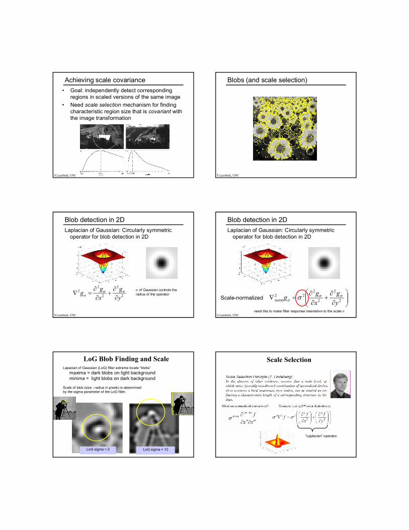
Scale-space blob detector: Example
S.Lazebnik, UNC
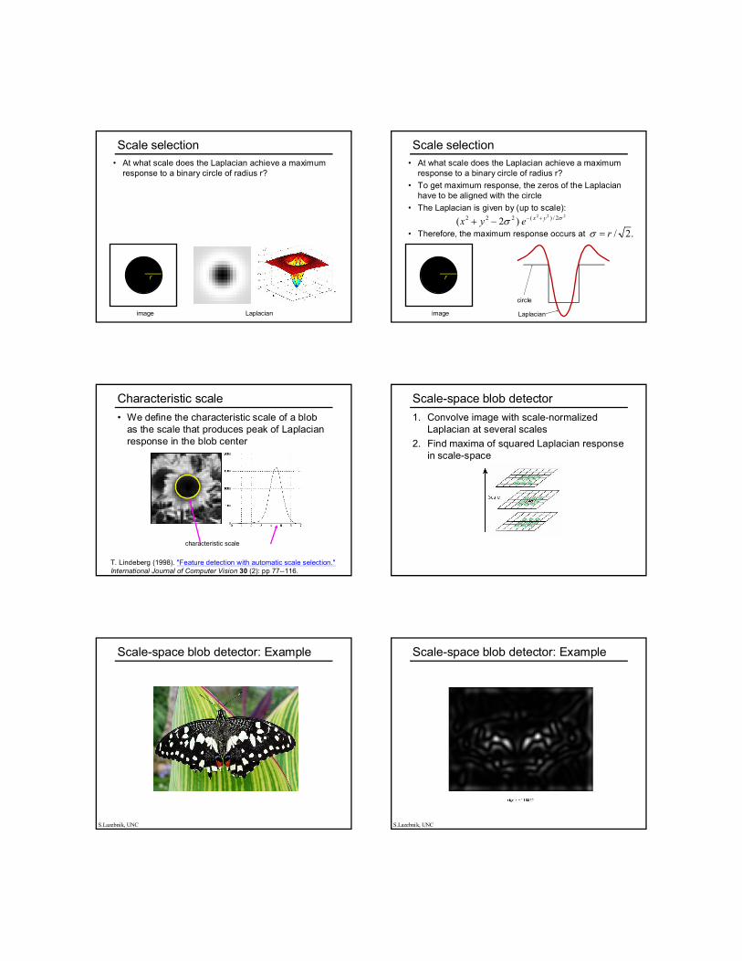
Scale-space blob detector: Example
S.Lazebnik, UNC
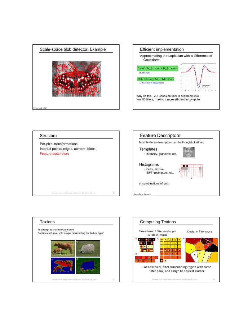
Scale-space blob detector: Example
S.Lazebnik, UNC
Approximating the Laplacian with a difference of Gaussians:
2 ( , , ) ( , , )xx yyL G x y G x y
( , , ) ( , , )DoG G x y k G x y
(Laplacian)
(Difference of Gaussians)
Efficient implementation
Why do this: 2D Gaussian filter is separable into two 1D filters, making it more efficient to compute.
Structure
1515Computer vision: models, learning and inference. ©2011 Simon J.D. Prince
Per-pixel transformations
Interest points: edges, corners, blobs
Feature descriptors
Feature Descriptors
Templates• Intensity, gradients, etc.
Histograms• Color, texture,
SIFT descriptors, etc.
James Hays, Brown U.
Most features descriptors can be thought of either:
or combinations of both
Textons
An attempt to characterize texture
Replace each pixel with integer representing the texture ‘type’
17Computer vision: models, learning and inference. ©2011 Simon J.D. Prince
Computing Textons
Take a bank of filters and apply to lots of images
Cluster in filter space
For new pixel, filter surrounding region with same filter bank, and assign to nearest cluster
18Computer vision: models, learning and inference. ©2011 Simon J.D. Prince
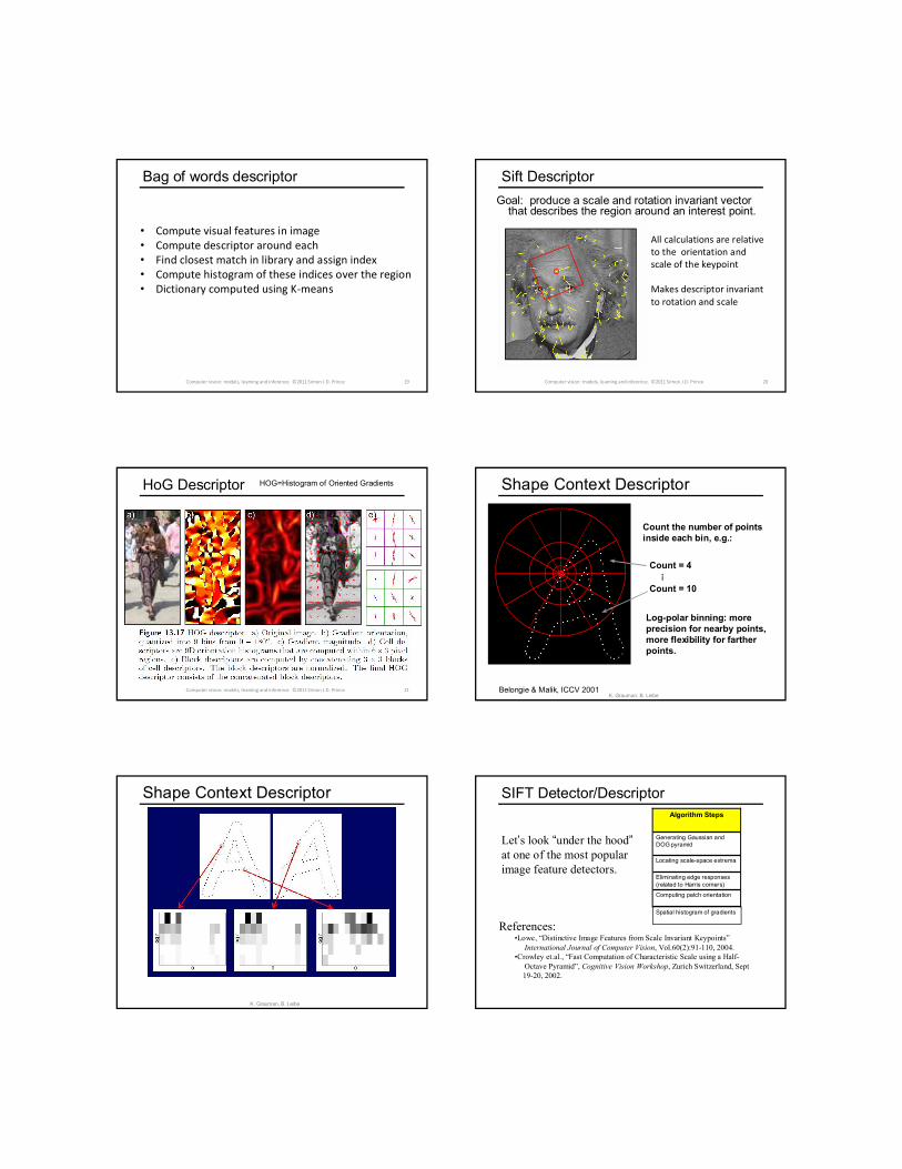
Bag of words descriptor
• Compute visual features in image • Compute descriptor around each• Find closest match in library and assign index• Compute histogram of these indices over the region• Dictionary computed using K-means
19Computer vision: models, learning and inference. ©2011 Simon J.D. Prince
Sift Descriptor
Goal: produce a scale and rotation invariant vector that describes the region around an interest point.
All calculations are relative to the orientation and scale of the keypoint
Makes descriptor invariant to rotation and scale
20Computer vision: models, learning and inference. ©2011 Simon J.D. Prince
HoG Descriptor
21Computer vision: models, learning and inference. ©2011 Simon J.D. Prince
HOG=Histogram of Oriented Gradients
Count the number of points inside each bin, e.g.:
Count = 4
Count = 10
...
Log-polar binning: more precision for nearby points, more flexibility for farther points.
Belongie & Malik, ICCV 2001K. Grauman, B. Leibe
Shape Context Descriptor
Shape Context Descriptor
K. Grauman, B. Leibe
SIFT Detector/DescriptorAlgorithm Steps
Computing patch orientation
Eliminating edge responses(related to Harris corners)
Locating scale-space extrema
Generating Gaussian and DOG pyramid
References:•Lowe, “Distinctive Image Features from Scale Invariant Keypoints”
International Journal of Computer Vision, Vol.60(2):91-110, 2004.•Crowley et.al., “Fast Computation of Characteristic Scale using a Half-
Octave Pyramid”, Cognitive Vision Workshop, Zurich Switzerland, Sept19-20, 2002.
Let’s look “under the hood”at one of the most popular image feature detectors.
Spatial histogram of gradients
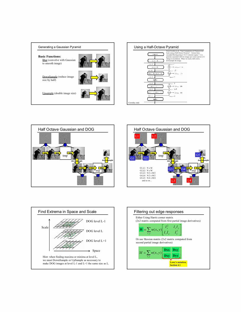
Generating a Gaussian Pyramid
Basic Functions:Blur (convolve with Gaussian to smooth image)
DownSample (reduce image size by half)
Upsample (double image size)
Using a Half-Octave Pyramid
Crowley etal.
From Crowley et.al., “Fast Computation of CharacteristicScale using a Half-Octave Pyramid.”. General idea:cascaded filtering using [1 4 6 4 1] kernel (sigma = 1) to generate a pyramid with two images per octave (power of 2 change in resolution). When we reach a full octave, downsample the image.
Half Octave Gaussian and DOG
blur blur
blur blur
downsample
blur
blur
downsample
tmp
tmp
Half Octave Gaussian and DOG
blur blur
blur blur
downsample
blur
blur
downsample
tmp
tmp
G1 G2
G3 G4
G5
L1 L2
L3 L4
G1,L1: N x MG2,L2: N x MG3,L3: N/2 x M/2G4,L4: N/2 x M/2G5,L5: N/4 x M/4
and so on…
Find Extrema in Space and Scale
Scale
Space
DOG level L-1
DOG level L
DOG level L+1
Hint: when finding maxima or minima at level L,we must DownSample or UpSample as necessary to make DOG images at level L-1 and L+1 the same size as L.
Filtering out edge responses
H
Either Using Harris corner matrix(2x2 matrix computed from first partial image derivatives)
Dxx Dxy
Dxy Dyy
Lowe’s notation,Section 4.1
Or use Hessian matrix (2x2 matrix computed fromsecond partial image derivatives)
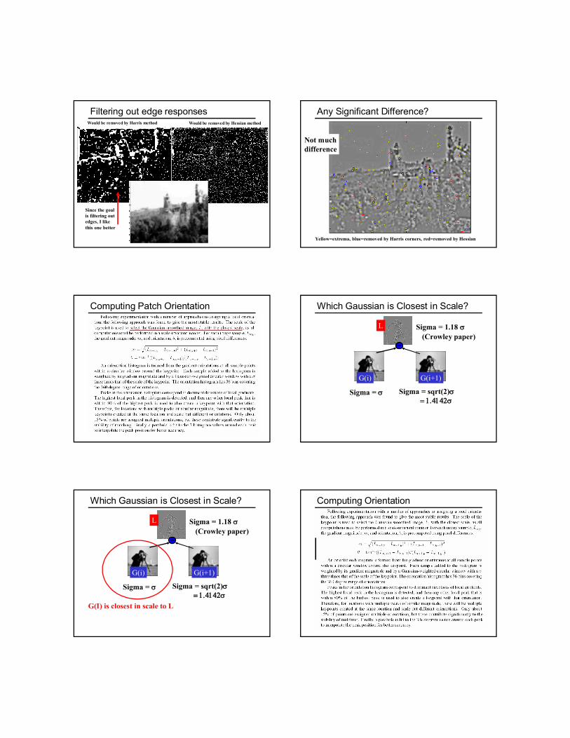
Filtering out edge responsesWould be removed by Harris method Would be removed by Hessian method
Since the goalis filtering outedges, I like this one better
Any Significant Difference?
Yellow=extrema, blue=removed by Harris corners, red=removed by Hessian
Not muchdifference
Computing Patch Orientation Which Gaussian is Closest in Scale?
G(i) G(i+1)
L
Sigma = Sigma = sqrt(2)
Sigma = 1.18 (Crowley paper)
Which Gaussian is Closest in Scale?
G(i) G(i+1)
L
Sigma = Sigma = sqrt(2)
Sigma = 1.18 (Crowley paper)
G(I) is closest in scale to L
Computing Orientation
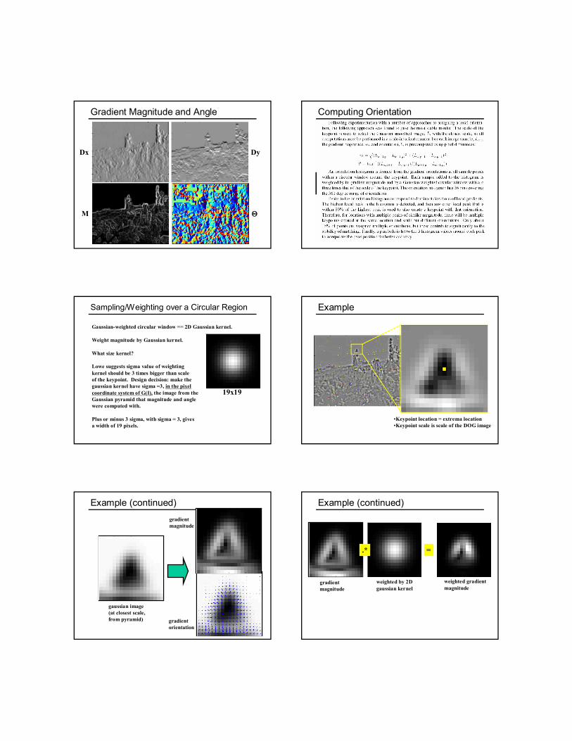
Gradient Magnitude and Angle
Dx Dy
M
Computing Orientation
Sampling/Weighting over a Circular Region
Gaussian-weighted circular window == 2D Gaussian kernel.
Weight magnitude by Gaussian kernel.
What size kernel?
Lowe suggests sigma value of weightingkernel should be 3 times bigger than scaleof the keypoint. Design decision: make thegaussian kernel have sigma =3, in the pixelcoordinate system of G(I), the image from theGaussian pyramid that magnitude and anglewere computed with.
Plus or minus 3 sigma, with sigma = 3, givesa width of 19 pixels.
19x19
Example
•Keypoint location = extrema location•Keypoint scale is scale of the DOG image
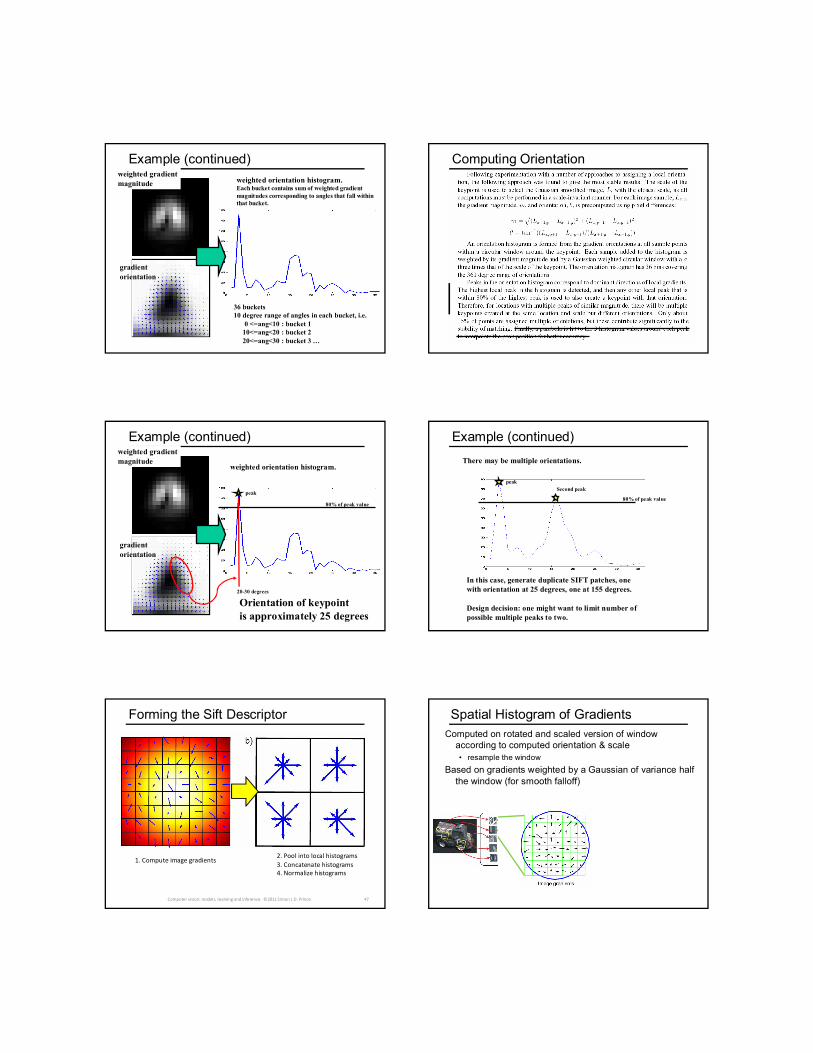
Example (continued)
gaussian image(at closest scale,from pyramid)
gradientmagnitude
gradientorientation
Example (continued)
gradientmagnitude
.* =
weighted by 2Dgaussian kernel
weighted gradientmagnitude
Example (continued)
gradientorientation
weighted gradientmagnitude weighted orientation histogram.
Each bucket contains sum of weighted gradient magnitudes corresponding to angles that fall within that bucket.
36 buckets10 degree range of angles in each bucket, i.e.
0 <=ang<10 : bucket 110<=ang<20 : bucket 220<=ang<30 : bucket 3 …
Computing Orientation
Example (continued)
gradientorientation
weighted gradientmagnitude
weighted orientation histogram.
80% of peak value
peak
20-30 degrees
Orientation of keypointis approximately 25 degrees
Example (continued)
There may be multiple orientations.
80% of peak value
peakSecond peak
In this case, generate duplicate SIFT patches, one with orientation at 25 degrees, one at 155 degrees.
Design decision: one might want to limit number of possible multiple peaks to two.
Forming the Sift Descriptor
1. Compute image gradients2. Pool into local histograms3. Concatenate histograms4. Normalize histograms
47Computer vision: models, learning and inference. ©2011 Simon J.D. Prince
Spatial Histogram of GradientsComputed on rotated and scaled version of window
according to computed orientation & scale• resample the window
Based on gradients weighted by a Gaussian of variance half the window (for smooth falloff)
Spatial Histogram of Gradients4x4 array of gradient orientation histograms
• each orientation “increment” is weighted by magnitude
8 orientations x 4x4 array = 128 dimensions
Motivation: some sensitivity to spatial layout, but not too much.
showing only 2x2 here but is 4x4
Ensure smoothness
Gaussian weight
Trilinear interpolation • a given gradient contributes to 8 bins:
4 in space times 2 in orientation
Reduce effect of illumination128-dim vector normalized to 1
Threshold gradient magnitudes to avoid excessive influence of high gradients• after normalization, clamp gradients >0.2
• renormalize
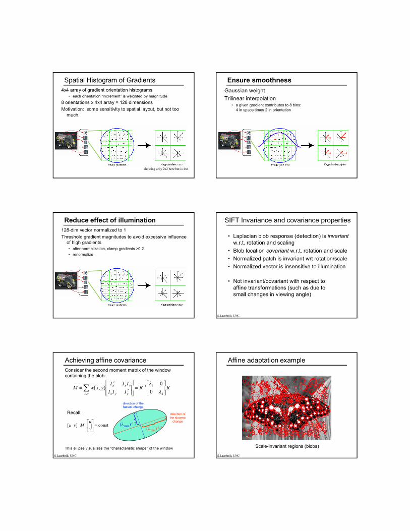
SIFT Invariance and covariance properties
• Laplacian blob response (detection) is invariantw.r.t. rotation and scaling
• Blob location covariant w.r.t. rotation and scale
• Normalized patch is invariant wrt rotation/scale
• Normalized vector is insensitive to illumination
• Not invariant/covariant with respect to affine transformations (such as due to small changes in viewing angle)
S.Lazebnik, UNC
Achieving affine covariance
RRIII
IIIyxwM
yyx
yxx
yx
2
112
2
, 0
0),(
direction of the slowest
change
direction of the fastest change
(max)-1/2
(min)-1/2
Consider the second moment matrix of the window containing the blob:
const][
v
uMvu
Recall:
This ellipse visualizes the “characteristic shape” of the window
S.Lazebnik, UNC
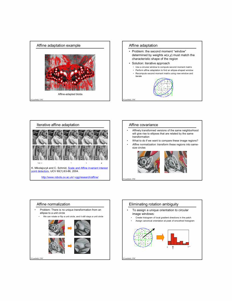
Affine adaptation example
Scale-invariant regions (blobs)
S.Lazebnik, UNC
Affine adaptation example
Affine-adapted blobs
S.Lazebnik, UNC
Affine adaptation
• Problem: the second moment “window”determined by weights w(x,y) must match the characteristic shape of the region
• Solution: iterative approach• Use a circular window to compute second moment matrix
• Perform affine adaptation to find an ellipse-shaped window
• Recompute second moment matrix using new window and iterate
S.Lazebnik, UNC
Iterative affine adaptation
K. Mikolajczyk and C. Schmid, Scale and Affine invariant interest point detectors, IJCV 60(1):63-86, 2004.
http://www.robots.ox.ac.uk/~vgg/research/affine/
Affine covariance• Affinely transformed versions of the same neighborhood
will give rise to ellipses that are related by the same transformation
• What to do if we want to compare these image regions?
• Affine normalization: transform these regions into same-size circles
S.Lazebnik, UNC
Affine normalization• Problem: There is no unique transformation from an
ellipse to a unit circle• We can rotate or flip a unit circle, and it still stays a unit circle
S.Lazebnik, UNC
Eliminating rotation ambiguity
• To assign a unique orientation to circular image windows:
• Create histogram of local gradient directions in the patch
• Assign canonical orientation at peak of smoothed histogram
0 2
S.Lazebnik, UNC
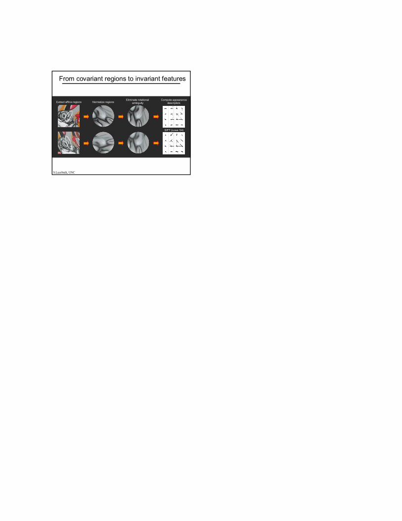
From covariant regions to invariant features
Extract affine regions Normalize regionsEliminate rotational
ambiguityCompute appearance
descriptors
SIFT (Lowe ’04)
S.Lazebnik, UNC