Embed Size (px)
Citation preview

iv
ACKNOWLEDGEMENT
First, I would like to give my sincere thanks to my advisor Dr. Kurt J. Marfurt, for his
guidance during my graduate study, it’s him who gave me so much encouragement
tostretch my potential, and whenever there were difficulties, there he was ready to help.
Also, his insight of geophysics enabled me to developinnovative problem solving ideas.
I want to extend my gratitude to my committee member Dr.Jamie Rich and Dr. Mitra
Shankar. Thanks for their comments and suggestions for my graduate research.
I thank the sponsors of the OU Attribute-Assisted Processing and Interpretation
Consortium for their financial support. I also thank BGP for permission to publish
showing their data.
I thank my family number, my parents, my elder sister and brother, my nephew and
my niece, for their selfless support to me since I was a child.
I thank theXuejun Wang, Zhonghong Wan of BGP., CNPC, for their advice during
the study.
I thank Deshuang Chang, Huailai Zhou, they taught me a lot, not only in study, but
also in the attitude for the world.
I thank the Chinese group of AASPI, Bo Zhang, ShiguangGuo, Tang Wang, Fangyu
Li, Tao Zhao, Jie Qi and JunxinGuo, for their being with me all the time, especially for
Bo Zhang, his wisdom and kindness make him be my idol.
I thank Brad Wallet, SumitVerma, MarcusCahoj, Thang Ha, Alfredo Fernandez,
Roderick Perez, OswaldoDavogustto, MeliadaSilva, Toan Dao, William Bailey and all
people who used to help me before.

v
I thank all the number of the Chinese Petroleum Association of Oklahoma, I believe
we will become strong club soon!

vi
Table of Contents
ACKNOWLEDGEMENTS ........................................................................................................... iv
TABLE OF CONTENTS ............................................................................................................... vi
LIST OF FIGURES ....................................................................................................................... viii
LIST OF TABLES ........................................................................................................................xiv
LIST OF SYMBOLS..................................................................................................................... xv
ABSTRACT ..................................................................................................................................xvi
Chapter 1 INTRODUCTION .......................................................................................................... 1
Chapter 2 PITFALLS IN ATTRIBUTE ANALYSIS IN STRUCTURALLY
COMPLEX AREAS ........................................................................................................................ 7
2.1 Fault Shadow ............................................................................................................................. 7
2.2 Velocity Push Down (Pull Up) ................................................................................................ 12
Chapters 3 ATTRIBUTE ACCURACY AND RESOLUTION AS A FUNCTION OF
THE VERTICAL ANALYSIS WINDOW ................................................................................... 14
3.1 A Review of Volumetric Dip Estimation ................................................................................ 14
3.2 A Review of Coherence........................................................................................................... 30
Chapter 4 THE EFFECT OF DIP ON SPECTRAL DECOMPOSITION .................................... 39
4.1 Spectral Decomposition........................................................................................................... 39
4.2 Dip Compensation ................................................................................................................... 42
Chapter 5 ATTRIBUTE ANALYSIS OF TIME- VS. DEPTH-MIGRATED DATA.................. 49

vii
5.1 Geologic Overview.................................................................................................................. 49
5.2 Seismic Data Quality and Data Conditioning ......................................................................... 52
5.3 Interpretational Advantages and Disadvantages of Depth-Migrated Data .............................. 60
5.3.1 Coherence with Self-adaptive Window ................................................................................ 68
5.3.2 Spectral Analysis with Dip Compensation ........................................................................... 73
5.3.3Seismic Interpretation............................................................................................................ 74
Chapter 6 CONCLUSIONS .......................................................................................................... 86
REFFERENCES ............................................................................................................................ 88

viii
LIST OF FIGURES
Figure 2.1 (a) The velocity model used to obtain synthetic data. (b) Time migrated
section showing near-vertical axes which link the time anomalies along each. ............................. 7
Figure 2.2 Vertical slices through (a) time- and (b) depth-migrated amplitude volumes ............... 9
Figure 2.3 Vertical slices though coherence co-rendered with seismic amplitude for (a)
time - and (b) depth-migrated data. (c) The velocity model for the zone indicated by the
red arrow in (a) and (b).................................................................................................................. 11
Figure 2.4 Vertical slices through co-rendered most-positive (k1) and most negative
(k2) principal curvatures and slice with (a) time migrated and (b) depth migrated
amplitude volumes......................................................................................................................... 12
Figure 3.1 The definition of volumetric dip. ................................................................................. 14
Figure 3.2 A schematic diagram of time window for dip and coherence computation. ................ 17
Figure 3.3 Schematic showing 2D dip calculation ........................................................................ 20
Figure 3.4 The proposed workflow to estimate a self-adaptive window for seismic
attribute calculation. ...................................................................................................................... 22
Figure 3.5 (a) The time migrated seismic trace and corresponding (b) time-frequency
spectrum (in cycles/s or Hz). (c) The original (blue curve) peak frequency overlain by
the smoothed (red curve) peak frequency. (d) The corresponding original (blue curve)
self-adaptive window size (m s) overlain by the smoothed (red curve) self-adaptive
window size (ms)........................................................................................................................... 23
Figure 3.6 (a) The depth migrated seismic trace and (b) corresponding depth-
wavenumber spectrum in cycles/km. (c) The original (blue curve) overlain by the

ix
smoothed (red curve) peak wavenumber. (d) The corresponding original (blue curve)
self-adaptive window size in km overlain by the smoothed (red curve) self-adaptive
window size. .................................................................................................................................. 24
Figure 3.7 (a) Time slice at I=0.6 s and (b) vertical slice AA’ through the seismic
amplitude volume. The white arrow in (a) indicates fault FF’ in (b). ........................................... 25
Figure 3.8 (a) Peak frequency co-rendered with seismic amplitude at t=0.6 s and (b)
vertical slice AA’ through the smoothed peak frequency volume corresponding to the
seismic data of Figure 3.7. The colored arrows indicate the channels shown in Figure
3.7 .................................................................................................................................................. 26
Figure 3.9 Time slices at t=0.6 s through the inline dip component computed using (a) a
fixed 20 ms window and (b) a self-adaptive window ranging between 10 and 40 ms.
Corresponding time slices through crossline dip components computed using (c) a fixed
20 ms window and (d) a self-adaptive window ranging between 10 and 40 ms. .......................... 29
Figure 3.10 Schematic showing a 2D search-based estimate of coherence (green solid
lines are the boundary of the self-adaptive window ...................................................................... 31
Figure 3.11 Time slice at t=0.6 s through coherence computed using a fixed (a) 0 ms (b)
2 ms (c) 4 ms (d) 10 ms (e) 20 ms (f) 30 ms (g) 40 ms windows and (h) using a variable
self-adaptive window ranging between 10 and 40 ms. (i) - (p) are corresponding vertical
slices along line AA’ ..................................................................................................................... 38
Figure 4.1 (a) The impedance (b) reflectivity (c) synthetic seismic profile with 5 percent
random noise (d) peak frequency co-rendered with the seismic amplitude of (c) of the
wedge model.................................................................................................................................. 41

x
Figure 4.2 A schematic diagram showing differences in apparent thickness to the real
thickness, with respect to dip magnitude....................................................................................... 42
Figure 4.3 The percent change in apparent thickness ha/hr as a function of dip
magnitude, θ. ................................................................................................................................. 44
Figure 4.4 (a) A thin bed model showing a layer with flat dip, strong negative dip and
moderate positive dip; (b) The real (marked by red line) tuning frequency (the apparent
tuning frequency is 50 Hz) of the layer. ........................................................................................ 45
Figure 4.5 (a) A thin bed model showing a layer with flat dip, strong negative dip and
moderate positive dip; (b) The real (marked by red line) tuning frequency (the real
tuning frequency is 50 Hz) of the layer. ........................................................................................ 46
Figure 4.6 The schematic diagram of apparent frequency (yellow line) and real
frequency (orange line).................................................................................................................. 46
Figure 4.7 The flowchart for spectral decomposition using matching pursuit algorithm
(after Liu and Marfurt, 2008) and compensation for structural dip. ............................................. 48
Figure 5.1 The location of the seismic survey............................................................................... 49
Figure 5.2 Stratigraphic column .................................................................................................... 50
Figure 5.3 The evolution of rift basin............................................................................................ 51
Figure 5.4 Time-structure map of the H1 horizon showing the location of vertical lines
AA’, BB’, and CC’. ....................................................................................................................... 52
Figure 5.5 Time- (a) vs. depth- (b) migrated data along line AA’ ................................................ 53
Figure 5.6 Vertical slices along line AA’’ through (a) time- and (b) depth-migrated
amplitude volumesbefore SOF (Structural Oriented Filter) .......................................................... 55

xi
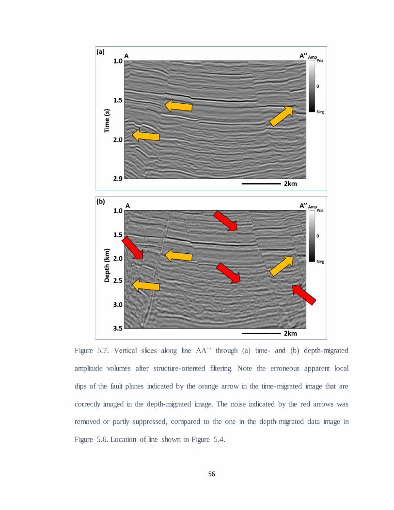
Figure 5.7 Vertical slices along line AA’’ through (a) time- and (b) depth-migrated
amplitude volumes after SOF (Structural Oriented Filter) ............................................................ 56
Figure 5.8 Vertical slices of rejected noise along line AA’’ through (a) time- and (b)
depth-migrated amplitude volumes before SOF (Structural Oriented Filter) ............................... 57
Figure 5.9 Vertical slices along line AA’’ through (a) time- and (b) depth-migrated
amplitude volumes with structural oriented filter ......................................................................... 58
Figure 5.10 Vertical slice though most positive curvature co-rendered with seismic
amplitude along line AA’’ for (a) time – and (b) depth – migrated data. ..................................... 61
Figure 5.11 Vertical slice though most positive curvature co-rendered with seismic
amplitude along line AA’’ for (a) time – and (b) depth – migrated data ...................................... 62
Figure 5.12 Vertical slice though most positive curvature co-rendered with most
negative curvature (with short wavelet) and seismic amplitude along line AA’’ for (a)
time – and (b) depth – migrated data. ............................................................................................ 63
Figure 5.13 Vertical slice though most positive curvature co-rendered with most
negative curvature (with midum wavelet) and seismic amplitude along line AA’’ for (a)
time – and (b) depth – migrated data. ............................................................................................ 64
Figure 5.14 Vertical slice though most positive curvature co-rendered with most
negative curvature (with long wavelet) and seismic amplitude along line AA’’ for (a)
time – and (b) depth – migrated data. ............................................................................................ 65
Figure 5.15 Vertical slice though coherence co-rendered with seismic amplitude along
line AA’’ for (a) time – and (b) depth – migrated data ................................................................. 66
Figure 5.16 Seismic profile of (a) time - and (b) depth - migrated data. (c) Depth
migrated data with interpreted faults and horizons. ...................................................................... 69
xii
Figure 5.17 Peak (a) frequency of time - and (b) peak wavenumber of depth - migrated
data. ............................................................................................................................................... 70
Figure 5.18 Vertical slices along Line AA’’ through coherence volumes computed from
time-migrated data using a (a) fixed height 20 ms analysis window and (b) a self-
adaptive window. Corresponding vertical slices through coherence volumes computed
from depth-migrated data using a (c) fixed height 40 ms analysis window and (d) a self-
adaptive window............................................................................................................................ 73
Figure 5.19 Peak frequency co-rendered with seismic amplitude of (a) time - and (b)
depth -migrated data. ..................................................................................................................... 75
Figure 5.20 Smoothed peak frequency blended with seismic amplitude of (a) time
migrated data and (b) depth migrated data. ................................................................................... 76
Figure 5.21 Dip compensation (1/cos𝜃) blended with seismic amplitude of (a) time -
and (b) depth - migrated data......................................................................................................... 77
Figure 5.22 Dip corrected peak frequency co-rendered with seismic amplitude of (a)
time - and (b) depth - migrated data. ............................................................................................. 79
Figure 5.23 Smoothed (with petrel), dip-corrected peak frequency blended with seismic
amplitude of (a) time - and (b) depth - migrated data. .................................................................. 80
Figure 5.24 (a) Time - migrated data and time migrated shown horizons (b) H1 (c) H2
and (d) H3. ..................................................................................................................................... 81
Figure 5.25 Time structure map of horizon H1 and H2 of the time –migrated data. .................... 82
Figure 5.26 Structure map of horizon H1 and H2 of the depth – migrated data. .......................... 82
Figure 5.27Coherence along horizon H4 and H5 of the time migrated data ................................. 83
Figure 5.28Coherence along horizon H4 and H5 of the depth migrated data ............................... 83

xiii
Figure 5.29Most positive curvature co-rendered with most negative curvature and
seismic amplitude along horizon H4 and H5 of the time migrated data ....................................... 84
Figure 5.30Most positive curvature co-rendered with most negative curvature and
seismic amplitude along horizon H4 and H5 of the depth migrated data ..................................... 85

xiv
LIST OF TABLES
Table 1.1 Attribute comparison of time- vs. depth-migrated data. ................................................. 3
Table 5.1 Seismic data parameters. ............................................................................................... 50

xv
LIST OF SYMBOLS
The table below summarizes the notation used in this thesis:
Symbols meaning
p, θx Inline apparent dips
q, θy Crossline apparent dips
θ Dip magnitude
ψ Dip strike
v Constant velocity during dip estimation
𝜱 Instantaneous phase
𝑢(𝑡, 𝑥, 𝑦) The input seismic data
𝑢𝐻(𝑡, 𝑥, 𝑦) Hilbert transform with respect to time t
𝜔, 𝑘𝑡 Instantaneous frequency
𝑘𝑥,𝑘𝑦 , 𝑘𝑧 Instantaneous wavenumber
ϕ Dip azimuth
vP P-wave velocity
fpeak Peak frequency in time domain
λpeak Peak wavenumber in depth domian
𝐻𝑔𝑎𝑡𝑒 Half window height
hr Real thickness of a dipping layers
ha Apparent thickness of a dipping layers
Vpa Phase velocity of apparent frequency
Vpr Phase velocity of real frequency
fa Apparent tuning frequency
fr Real tuning frequency

xvi
ABSTRACT
Most seismic attributes were originally designed and tested on time-migrated data.
While many papers show the value of attribute analysis of depth-migrated volumes, few
have compared the images to corresponding time-migrated volumes.I therefore use
time- and depth-migrated volumes of RenqiuField to show not the only the value of
depth-migration, but the necessary data-conditioning, algorithmic modification, and
interpretation workflow of attributes computed from depth data.
Since one of the goals of depth migration is to image steep dips, one also allows
steeply dipping noise to overprint the image. I suppress this noise through careful
structure-oriented filtering. Fault plane reflections are also imaged by depth migration
and gives rise to dips that conflict with those of the underlying reflectors.
In depth-migrated data, spectral components are now measured in cycles/km
(wavenumber) rather than in cycles/s or Hertz (frequency). While smoothly varying
velocity models used in Kirchhoff depth migration give rise to smoothly varying
wavenumber stretch, discontinuous velocity models used in wave equation and reverse
time migration will give rise to wavenumber artifacts straddling the velocity
discontinuity boundary. Furthermore, imaging of steep dips results in a shift by cosθ of
true to lower apparent spectral components.
Ideally, vertical attribute analysis windows should be kept as small as the data allow,
with windows scaled to be some fraction of the dominant wavelength. Since the size of
the dominant wavelength changes as a function of velocity in depth-migrated data, a
single fixed-sized window may be too large for shallower data and too small for deeper
data.

xvii
I address these changes through several simple modifications to the attribute
algorithms. First, I rescale the spectral components by 1/cosθ using an attribute estimate
of local dip magnitude. Second, I construct data-adaptive vertical analysis windows
based on the dominant (peak) frequency (or wavenumber) measured at each voxel.
I demonstrate the value of these algorithmic modifications to a survey acquired over the
carbonate Renqiu oil field in Hebei Province China. The complex faulting gives rise to
a laterally variable velocity,so that depth migration of the data is necessary. After data
conditioning, I obtain a clean relatively noise-free, well-focused depth-migrated image.
Artifacts in the time-migrated data such as fault shadows giving rise to coherence
anomalies and velocity pull-up and push-down giving rise to curvature anomalies.
These artifacts are minimized in the depth-migrated data. Deeper data are better focused
in the depth-migrated that time-migrated data, resulting in sharper coherence images are
sharper, and a more accurate image of the fault network in the depth-migrated data.
Finally, structural features such as folds and flexures are directly linked to the depth-
structure of the data via the laterally variable velocity model.

1
Chapter 1 INTRODUCTION
Seismic attributes are often used to extract subtle features in seismic data that can be
used to map structural deformation and depositional environment. While instantaneous
attributes and spectral components are computed trace by trace, most other attributes are
“structure-oriented” and as such require an initial estimate of reflector dip and azimuth.
Picou and Utzman (1962) introduced dip estimation into 2D seismic interpretation.
Finn and Backus (1986) extended dip estimation to 3D as a piecewise continuous function
of spatial position and seismic traveltime. Cerveny and Zahradnik (1975) and (Taner et
al., 1979) showed how the Hilbert transform can be used to calculate complex traces of
seismic data which can then be used to estimate instantaneous frequency. Luo et al. (1996)
computed instantaneous wavenumbers in the inline and crossline direction, thereby
enabling a 3D estimate of vector dip. Barnes (2000) showed how smoothing the
instantaneous phase and wavenumbers by the envelope provides a significantly more
stable estimate of 3D dip. Marfurt et al. (1998) used a simple semblance search to
estimate dip and azimuth, which was further improved by subsequent mean or median
filters. In an edge-preserving smoothing application, Luo et al., (2002) applied Kuwahara
et al., (1976)’s multiwindow analysis by smoothing in windows that did not straddle
discontinuities measured as having high standard deviation. Marfurt (2006) modified this
approach for volumetric dip calculations where he used coherence as a measure of
discontinuities and 3D rather than 2D overlapping windows.
Coherence is a multitrace estimate of reflector continuity and is routinely used to map
structural and stratigraphic edges. Coherence should always be computed along structural
dip. Bahorich and Farmer (1995) introduced the first coherence algorithm by computing
2
the geometric mean of the maximum cross-correlation coefficients in the inline and
crossline directions. Marfurt et al. (1998) improved upon this method by using a 5-, 9-,
or greater trace semblance-based coherence algorithm, which improved the signal-to-
noise noise ratio over the three-trace algorithm but reduced the lateral resolution.
Gersztenkorn and Marfurt (1996, 1999) offered the third-generation algorithm based on
calculating the eigenvalues and eigenvectors of the covariance matrix. In principle, cross–
correlation and eigenstructure based coherence algorithms, including “chaos” based on
the gradient structure tensors, (von Bemmel and Pepper, 2011) are sensitive only to
changes in the seismic waveform, while semblance, variance, and Sobel filter coherence
(Luo et al., 1996) algorithms are sensitive to both changes in amplitude and waveform.
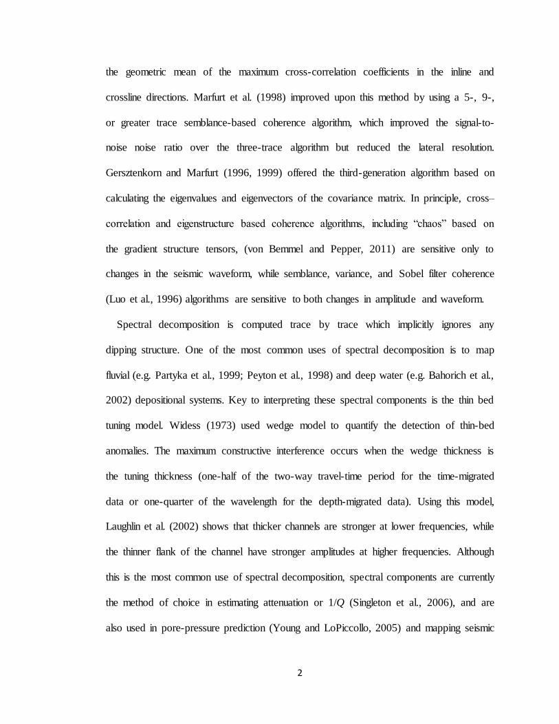
Spectral decomposition is computed trace by trace which implicitly ignores any
dipping structure. One of the most common uses of spectral decomposition is to map
fluvial (e.g. Partyka et al., 1999; Peyton et al., 1998) and deep water (e.g. Bahorich et al.,
2002) depositional systems. Key to interpreting these spectral components is the thin bed
tuning model. Widess (1973) used wedge model to quantify the detection of thin-bed
anomalies. The maximum constructive interference occurs when the wedge thickness is
the tuning thickness (one-half of the two-way travel-time period for the time-migrated
data or one-quarter of the wavelength for the depth-migrated data). Using this model,
Laughlin et al. (2002) shows that thicker channels are stronger at lower frequencies, while
the thinner flank of the channel have stronger amplitudes at higher frequencies. Although
this is the most common use of spectral decomposition, spectral components are currently
the method of choice in estimating attenuation or 1/Q (Singleton et al., 2006), and are
also used in pore-pressure prediction (Young and LoPiccollo, 2005) and mapping seismic

3
discontinuities (Davogustto et al., 2013), as well as some implementations of seismic
chronostratigraphy.
Table 1.1. Attribute comparison of time- vs. depth-migrated data.
Seismic attributes have been applied to depth-migrated data since their inception;
however, few authors have addressed the pitfalls in the attribute interpretation of depth –
migrated data. Fewer authors still have addressed the modification in computation or
interpretation workflow in using depth- vs. time- migrated data.
Stop
Caution
Go
Interpretation traffic light

4
Rietveld et al. (1999) showed the difference in coherence, coherent energy, and
coherent energy gradients on prestack depth-migrated vs. time-migrated data for surveys
acquired offshore Trinidad and the Netherlands. Counter intuitively, their Trinidad
coherence images were less coherent, due to the imaging of very closely spaced (25 m in
6.5-bin data) broad fault zones. By more accurately accounting for ray bending at far
offset, prestack depth migration also provided superior imaging with little lateral
variation of flat-lying overburden above polygonal shale “dewatering” features seen in
coherence and coherent energy gradients.
In general, depth migration is necessary in the presence of strong lateral velocity
variation and avoids some of the pitfalls that occur in time-migrated data (Table 1.1).
First, fault shadows can give rise to a second (artificial) coherence anomaly on time-
migrated data. Such artifacts are removed in accurate velocity depth-migrated data.
Second, velocity pull-up and push-down caused by the lateral changes in the overburden
such as carbonate buildups and incised valleys will give rise to erroneous curvature
anomalies in time-migrated data. These artifacts disappear in properly depth-migrated
data. Third, in complex structure time-migrated data may be poorly focused. Fault
termination of reflectors may be misaligned, giving rise to “wormy” coherence
anomalies. Channel and other stratigraphic features may be diffuse (as reported by
Rietveld et al., 1999) making them hard to interpret.
Depth-migrated data presents its own challenges. In time migration, moderate changes
in the velocity focus or defocus reflectors and diffractors and result in some lateral
movement. In depth migration, such changes can result in significant lateral and vertical
movement. If the velocity model is inaccurate, depth migration may be inferior to time-

5
migrated data. Even if the data are properly imaged, the wavelet spectrum is no longer in
Hertz, but in vertical wavenumber (the reciprocal of the apparent vertical wavelength)
which decreases with the increase of velocity with depth.
Since the dominant wavelength increases with increasing velocity which in turn
increases with depth, attributes such as coherence benefit by using shorter vertical
analysis windows in the shallow section and longer vertical analysis windows in the
deeper section. Most coherence implementations require a fixed vertical analysis
window. To address the change in wavelength with depth, the interpreter simply runs the
algorithm using an appropriate window for each zone to be analyzed. Curvature is
naturally computed in the depth domain, with most algorithms requiring a simple
conversion velocity for time-migrated data. For more accurate results, the interpreter uses
different conversion velocities for different target depths, or simply converts the entire
volume to depth using well control. Both coherence and curvature are structurally driven
algorithms, with coherence computed along structural dip and curvature computed from
structural dip.
I begin this thesis in Chapter 2 with a review of common pitfalls encountered in
applying seismic attributes to data that have not been properly migrated. In Chapter 3, I
discuss the effect of a fixed-height vertical analysis window on depth-migrated data and
introduce a data-adaptive analysis window based on the local dominant frequency at each
voxel. Chapter 4 shows the effect of dip on spectral components, and shows how the
apparent spectrum can be converted to a better approximation of the true spectrum by
using local estimates of volumetric dip. Chapter 5 illustrates some of the pitfalls shown
in Chapter 2 and algorithmic improvements introduced in Chapters 3 and 4 to Renqiu
6
Field, where I use attributes to quantitatively show the value of depth-migrated vs. time-
migrated images. Finally, in Chapter 6 I provide a brief summary of my findings and
suggestions for future work.

7
Chapter 2 PITFALLS IN ATTRIBUTE ANALYSIS IN
STRUCTURALLY COMPLEX AREAS
2.1. Fault Shadow
Coherence algorithm measure lateral changes in seismic waveform. (Bahorich and
Farmer, 1995, 1996). Like other attributes, coherence is sensitive to noise. To avoid this
problem, Kirlin (1992), Marfurt et al. (1998), Gersztenkorn (1997), and Gersztenkorn and
Marfurt (1996a, 1996b, 1999) introduced more robust multitrace semblance- and
eigenstructure-based coherence algorithms which provided improved images in the
presence of random noise.
In contrast to random noise, all coherence algorithms are sensitive to fault shadows
seen in time-migrated data. Fagin (1991) uses forward ray trace modeling to illustrate the
fault shadow problem. Fault whisper Hatchell (2000) is the phenomenon of transmission
distortions, which are produced by velocity changes across buried faults and
unconformities and related to the phenomenon known as fault shadows.
Figure 2.1. (a) The velocity model used to obtain synthetic data. High velocities horizon
are indicated in yellow. (b) Time-migrated section showing near-vertical axes, which link
the time anomalies along each reflection (Fagin, 1991).

8
Looking in detail at these oscillations in Figure 2.1b, we can identify the Queen City
Sag, the Reklaw Pull-up, and the Wilcox Sag. On the time section a near-vertical
structural axis can be drawn which links the position of each of these anomalies for each
underlying reflection. These axes are a predictable consequence of extensional faulting
of the sequence of velocity units that occur in this study area. In the real data example
presented later they are shown to occur in each fault block (Fagin, 1991).

9
Figure 2.2. Vertical slices through (a) time- and (b) depth-migrated amplitude volumes.
Green dotted line indicates the fault and orange dotted line the fault shadow.
Figures 2.2a and b show vertical slices through of time- and depth-migrated amplitude
volumes acquired over Renqiu Field, China. All main faults are normal faults. The yellow
solid lines in Figure 2.2a and b show us the horizons, where a structural high near the
fault in Figure 2.2a is generated. The red arrow in Figure 2.2a at the top of a high velocity
carbonate formation indicate the initiation of the fault shadow shown as an orange dotted
line, which gives rise to a false structural high. This is because they are at upthrow, which
means they should be structural low zone. In the depth-migrated data in Figure 2.2b, the
fault shadows are gone and the structure becomes flatter.
The data shown in Figure 2.2 have been windowed and scaled to show approximately
the same geology. In principal, the depth-migrated image should be “better”. The most
striking difference between the two images are the strong fault-plane reflections seen in
Figure 2.2b. These fault planes line up nicely with the reflector terminations, indicating
that we have little to no anisotropy.
Unfortunately, there are other steeply dipping features which are migration edge of
survey artifacts that are particularly strong on the left and right hand sides of the survey.
The ability to image steep dip also results in increased migration operator aliasing, which
overprints weaker reflectors in the lower middle part of the survey, making them appear
less coherent.

10

11
Figure 2.3. Vertical slices though coherence co-rendered with seismic amplitude for (a)
time - and (b) depth-migrated data. (c) The velocity model for the zone indicated by the
red arrow in (a) and (b).
Coherence is an important aid in fault interpretation. Figure 2.3a shows low coherence
fault shadows indicated by the red arrow in the time-migrated data. This wide low-
coherence zone is removed in the depth-migrated data shown in Figure 2.3b. Figure 2.3c
is a cartoon of the velocity model corresponding to the zone indicated by the red arrow
in Figures 2.3a and b.

12
2.2. Velocity Push-down (Pull-up)
Figure 2.4. Vertical slices through co-rendered most-positive (k1) and most negative (k2)
principal curvatures co-rendered with (a) time-migrated and (b) depth-migrated
amplitude volumes. Red and blue arrows indicate subtle velocity pull-up and push-down
in the time-migrated data volumes.
I co-render the most-positive curvature, most-negative curvature, and seismic
amplitude of time-migrated and depth-migrated data in Figure 2.4. The white arrow in

13
Figure 2.4a indicates a positive curvature zone (indicated by the red arrow) and a negative
curvature zone (indicated by the blue arrow), which are no longer apparent in Figure 2.4b
where depth migration flattens the horizon.

14
Chapters 3 ATTRIBUTE ACCURACY AND RESOLUTION AS A
FUNCTION OF THE VERTICAL ANALYSIS WINDOW
3.1. A Review of Volumetric Dip Estimation
Mathematically, a planar element of a seismic reflector can be defined uniquely by a
point in space, x = (x, y, z), and a unit normal to the surface, n = (nx, ny, nz), where nx, ny
and nz denote the components along the x, y and z axes, respectively, and are chosen such
that nz ≥ 0 (Figure 3.1).
Geologically, we define a planar interface such as a formation top or internal bedding
surface by means of apparent dips θx and θy, or more commonly, by the surface’s true dip
θ, and its strike, ψ (Figure 3.1).
Figure 3.1. The definition of volumetric dip. (After Marfurt, 2006).
Without knowing the velocity of the earth, we often find it convenient to measure the
apparent seismic (two-way) time dips, p and q, where p is the apparent dip measured in

15
s/km (or s/kft) in the inline, or x direction, and q is the apparent dip measured in s/km (or
s/kft) in the crossline, or y direction. If the earth can be approximated by a constant
velocity, v, the relationship between the apparent time-dips p and q, and the apparent
angle dips θx and θy, are:
𝑝 = 2tan𝜃𝑥 /𝑣 , and (3.1a)
q= 2tan𝜃𝑦 /𝑣 . (3.1b)
Using the Hilbert transform, we can compute the instantaneous phase, 𝜱
𝜱 = ATAN(𝑢𝐻 , 𝑢) , (3.2)
where 𝑢(𝑡, 𝑥, 𝑦) denotes the input seismic data, 𝑢𝐻 (𝑡, 𝑥, 𝑦) denotes its Hilbert transform
with respect to time t, and ATAN2 denotes the arctangent function whose output varies
between –𝜋 and +𝜋.
Using the chain rule, the instantaneous temporal frequency is then (Taner et al., 1979):
𝜔(𝑡, 𝑥, 𝑦) =𝜕𝜱
𝜕𝑡=
𝑢𝜕𝑢𝐻
𝜕𝑡−𝑢𝐻 𝜕𝑢
𝜕𝑡
(𝑢)2+(𝑢𝐻)2 . (3.3 a)
Generalizing the derivative to be in z for depth-migrated data as well as x and y, we
obtain the instantaneous wavenumbers, kz, 𝑘𝑥 and 𝑘𝑦
𝑘𝒙𝒋=
𝑑𝜱
𝑑𝑥𝑗=
𝑢𝑑𝑢𝐻
𝑑𝑥𝑗−𝑢𝐻 𝑑𝑢
𝑑𝑥𝑗
(𝑢)2+(𝑢𝐻 )2 , (3.3 b)
where xj takes on the values of x, y or z. Then the apparent dips are
𝜃𝑥=tan−1(𝑘𝑥 𝑘𝑧⁄ ) , and (3.4a)
𝜃𝑦=tan−1(𝑘𝑦 𝑘𝑧⁄ ) , (3.4b)
while the true dip and azimuth are
𝜃=tan−1 [(𝑘𝑥2 + 𝑘𝑦
2)1/2
𝑘𝑧⁄ ] , and (3.4c)

16
ϕ=ATAN2(𝑘𝑦 ,𝑘𝑥 ) . (3.4d)
Barnes (2000) found such estimates of instantaneous dips to be inaccurate. To improve
these estimates he first smoothed 𝜔, 𝑘𝑥, 𝑘𝑦 and 𝑘𝑧 using an envelope-weighted window
prior to application of equations 3.1 and 3.4.
Marfurt et al. (1998) and many others use a simple semblance search to estimate vector
dip. In Figure 3.2, the maximum coherence is calculated along the dip indicated by the
red dashed line. The peak value of this curve estimates coherence, while the dip value of
this peak estimates instantaneous dip. A more accurate estimate is obtained by passing a
parabolic surface through appropriate angles centered about the most coherent search
angle and computing its peak. The location of the peak provides an improved estimate of
the dip. Further improvements can be obtained by using multiple overlapping analysis
windows (Kuwahara et al., 1976; Marfurt, 2006).
Dip, coherence, and many other attribute analysis windows are best centered along dip
(Marfurt et al., 1999).

17
Figure 3.2. A schematic diagram of time window for dip and coherence computation.
For coherence computations, the window will be tapered, allowing windows of
fractional sample length.
Increase the radii (for elliptical windows) or length and width (for rectangular
windows) of the analysis window increases the computational cost. In contrast, by using
an “add/drop” construct in computing the numerator and denominator of the semblance
algorithm the window height does not significantly impact run times. However, larger
windows can result in vertical smearing, mixing shallower and deeper stratigraphic
features into the zone of interest. Since the seismic wavelet already mixes stratigraphy, a

18
good rule-of-thumb for noisy data is to use a vertical analysis windows on the order of
the dominant period or wavelength in the data, at least until we have the opportunity to
run structure-oriented filtering.
19
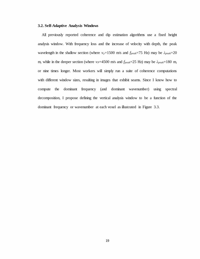
3.2. Self-Adaptive Analysis Windows
All previously reported coherence and dip estimation algorithms use a fixed height
analysis window. With frequency loss and the increase of velocity with depth, the peak
wavelength in the shallow section (where vp=1500 m/s and fpeak=75 Hz) may be λpeak=20
m, while in the deeper section (where vP=4500 m/s and fpeak=25 Hz) may be λpeak=180 m,
or nine times longer. Most workers will simply run a suite of coherence computations
with different window sizes, resulting in images that exhibit seams. Since I know how to
compute the dominant frequency (and dominant wavenumber) using spectral
decomposition, I propose defining the vertical analysis window to be a function of the
dominant frequency or wavenumber at each voxel as illustrated in Figure 3.3.

20
Figure 3.3. Schematic showing 2D dip calculation. (a) Coherence computed within fixed
windows that are rotated through candidate dips. The window with the highest coherence
(red dotted line) defines the approximate dip, which is improved by subsequent
interpolation. Green solid lines indicate the boundary of the self-adaptive window. Black
solid lines are the boundary of the user-defined constant window. (b) The same
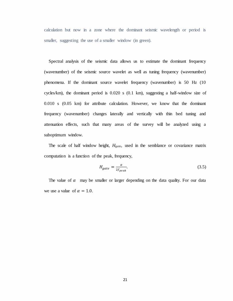
21
calculation but now in a zone where the dominant seismic wavelength or period is
smaller, suggesting the use of a smaller window (in green).
Spectral analysis of the seismic data allows us to estimate the dominant frequency
(wavenumber) of the seismic source wavelet as well as tuning frequency (wavenumber)
phenomena. If the dominant source wavelet frequency (wavenumber) is 50 Hz (10
cycles/km), the dominant period is 0.020 s (0.1 km), suggesting a half-window size of
0.010 s (0.05 km) for attribute calculation. However, we know that the dominant
frequency (wavenumber) changes laterally and vertically with thin bed tuning and
attenuation effects, such that many areas of the survey will be analyzed using a
suboptimum window.
The scale of half window height, Hgate, used in the semblance or covariance matrix
computation is a function of the peak, frequency,
𝐻𝑔𝑎𝑡𝑒 =𝛼
2𝑓𝑝𝑒𝑎𝑘. (3.5)
The value of 𝛼 may be smaller or larger depending on the data quality. For our data
we use a value of 𝛼 = 1.0.

22
Figure 3.4. The proposed workflow to estimate a self-adaptive window for seismic
attribute calculation.
23
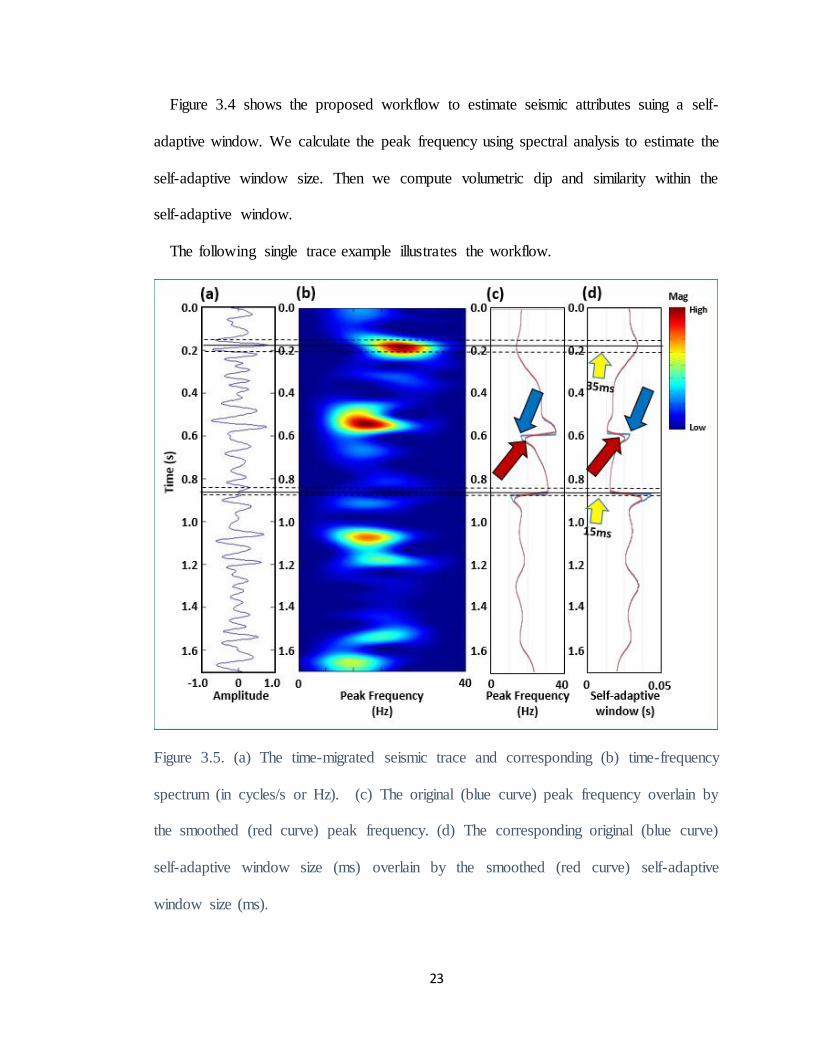
Figure 3.4 shows the proposed workflow to estimate seismic attributes suing a self-
adaptive window. We calculate the peak frequency using spectral analysis to estimate the
self-adaptive window size. Then we compute volumetric dip and similarity within the
self-adaptive window.
The following single trace example illustrates the workflow.
Figure 3.5. (a) The time-migrated seismic trace and corresponding (b) time-frequency
spectrum (in cycles/s or Hz). (c) The original (blue curve) peak frequency overlain by
the smoothed (red curve) peak frequency. (d) The corresponding original (blue curve)
self-adaptive window size (ms) overlain by the smoothed (red curve) self-adaptive
window size (ms).

24
Figures 3.5 and 3.6 show us the seismic trace, frequency (wavenumber) spectrum and
peak frequency (peak wavenumber) curves as well as the corresponding self-adaptive
window size of time-migrated data and depth-migrated data, respectively. Smoothing the
peak frequency (wavenumber) removes spurious values such as those indicated by the
blue arrow.
The yellow arrows in Figures 3.5 and 3.6 indicate the relevant self-adaptive window
size (s for time-migrated data; km for depth-migrated data). The self-adaptive size
matches the seismic trace very well.
Figure 3.6. (a) The depth-migrated seismic trace and (b) corresponding depth-
wavenumber spectrum in cycles/km. (c) The original (blue curve) overlain by the
smoothed (red curve) peak wavenumber. (d) The corresponding original (blue curve) self-

25
adaptive window size in km overlain by the smoothed (red curve) self-adaptive window
size.
To test the effect of varying window height I analyze the data shown in Figure 3.7
acquired over a fluvial system on the China shelf.
Figure 3.7. (a) Time slice at I=0.6 s and (b) vertical slice AA’ through the seismic
amplitude volume. The white arrow in (a) indicates fault FF’ in (b). The colored (red,
yellow, blue and orange) arrows indicate channels crossing the vertical slice AA’.
0

26
Figure 3.8. (a) Peak frequency co-rendered with seismic amplitude at t=0.6 s and (b)
vertical slice AA’ through the smoothed peak frequency volume corresponding to the
seismic data of Figure 3.7. The colored arrows indicate the channels shown in Figure
3.7.The white arrow F and FF’ indicate the fault.
Note the strong amplitude reflections (and some velocity push-down push-down) seen
in the channels. Figure 3.8 shows corresponding slices through the smoothed peak
frequency volume. The red, yellow and orange arrows in Figure 3.7 indicate a single
meandering channel that crosses line AA’ three times. This channel tunes in at about 30
Hz and appears as yellow-green in Figure 3.8 (indicated by colored arrows). In contrast,
0
0

27
the relatively straight channel indicated by the orange arrow in Figure 3.8 tunes in at
about 20 Hz and appears as the orange zone in Figure 3.8 (indicated by the purple arrow).
Consequently, the thickness of the meandering channel is a little thinner than the straight
channel.
We found that most of the data exhibit peak frequencies between 10 - 40 Hz.
Accordingly, we set the full analysis window to be 100 – 25 ms so that they contain a full
period.

28

29
Figure 3.9. Time slices at t=0.6 s through the inline dip component computed using (a) a
fixed 20 ms window and (b) a self-adaptive window ranging between 10 and 40 ms.
Corresponding time slices through crossline dip components computed using (c) a fixed
20 ms window and (d) a self-adaptive window ranging between 10 and 40 ms.
Figures 3.9a and b show time slices through the inline dip component computed with
constant 20 ms and variable vertical windows. Figures 3.9c and d show time slices
through the crossline dip for the same windows. Erratic dip estimates often occur when
there is crosscutting noise. Note that there are fewer erratic estimates in the upper left the
survey (red square zoomed in and plotted in to the lower right) with variable vertical
window.
30
3.2. A Review of Coherence
Coherence is a measure of similarity between waveforms or traces. When seen on a
processed section, the seismic waveform is a response of the seismic wavelet convolved
with the geology of the subsurface. That amplitude, frequency, and phase change depends
on the acoustic-impedance contrast and thickness of the layers above and below the
reflecting boundary. In turn, acoustic impedance is affected by the lithology, porosity,
density, and fluid type of the subsurface layers. Consequently, the seismic waveforms
that we see on a processed section differ in lateral character – that is, strong lateral
changes in impedance contrasts give rise to strong lateral changes in waveform character.
Figure 3.10 is a schematic diagram showing the steps used in semblance estimation of
coherence. First, we calculate the energy of the five input traces (black curves) within an
analysis window, then we calculate the average trace (red curves), and finally, we replace
each trace by the average trace and calculate the energy of the five average traces. The
semblance is the ratio of the energy of the coherent (averaged or smoothed) traces to the
energy of the original (unsmoothed) traces.

31
Figure 3.10. Schematic showing a 2D search-based estimate of coherence (green solid
lines are the boundary of the self-adaptive window. The window in (b) is larger than the
window in (a) since the wavelet is longer.
Figure 3.10 also provides a schematic of the coherence estimation using self-adaptive
windows, where the window in Figure 3.6 is narrower compared to the one the Figure
3.10 b.

32
For a fixed level of noise, the signal-to-noise ratio can become low near reflector zero
crossings, thereby resulting in low-coherence artifacts that follow the structure (arrows).
Using the analytic trace avoids this problem, since the magnitude of the real input trace
is low when the magnitude of the Hilbert transform component is high. Likewise, when
the magnitude of the Hilbert transform component is low, the magnitude of the real input
trace is high, thereby maintaining a good signal-to-noise ratio in the presence of strong
reflectors (as measured by the envelope). Low-coherence trends follow structure when
we have low-reflectivity (and hence low signal-to-noise ratio) shale-on-shale events, and
when we have truly incoherent geology such as that encountered with erosional and
angular unconformities, or when we encounter karst, mass-transport complexes, and
turbidities.

33

34

35
36

37
38
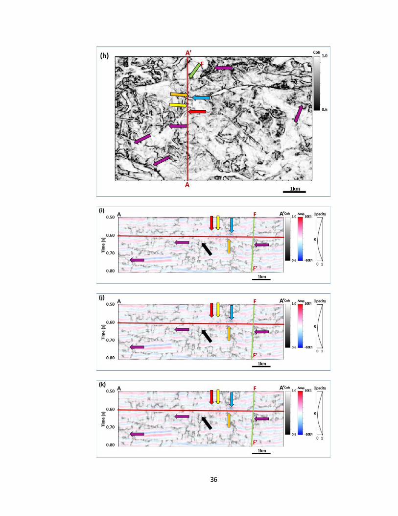
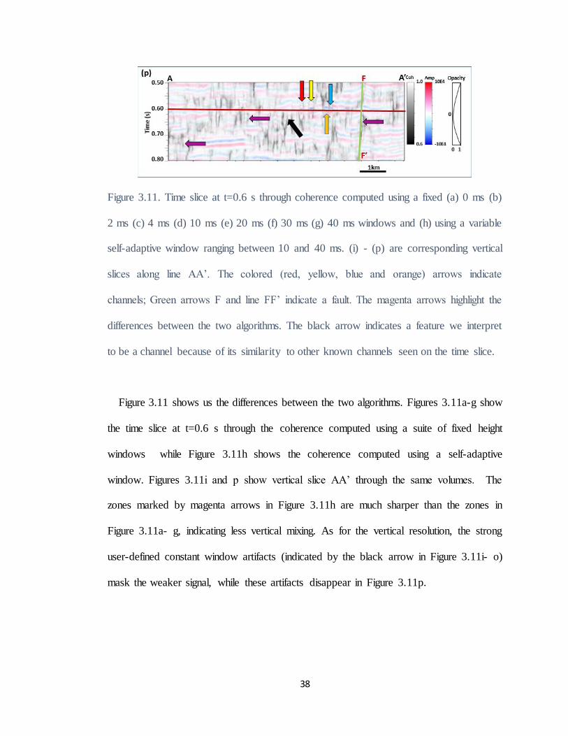
Figure 3.11. Time slice at t=0.6 s through coherence computed using a fixed (a) 0 ms (b)
2 ms (c) 4 ms (d) 10 ms (e) 20 ms (f) 30 ms (g) 40 ms windows and (h) using a variable
self-adaptive window ranging between 10 and 40 ms. (i) - (p) are corresponding vertical
slices along line AA’. The colored (red, yellow, blue and orange) arrows indicate
channels; Green arrows F and line FF’ indicate a fault. The magenta arrows highlight the
differences between the two algorithms. The black arrow indicates a feature we interpret
to be a channel because of its similarity to other known channels seen on the time slice.
Figure 3.11 shows us the differences between the two algorithms. Figures 3.11a-g show
the time slice at t=0.6 s through the coherence computed using a suite of fixed height
windows while Figure 3.11h shows the coherence computed using a self-adaptive
window. Figures 3.11i and p show vertical slice AA’ through the same volumes. The
zones marked by magenta arrows in Figure 3.11h are much sharper than the zones in
Figure 3.11a- g, indicating less vertical mixing. As for the vertical resolution, the strong
user-defined constant window artifacts (indicated by the black arrow in Figure 3.11i- o)
mask the weaker signal, while these artifacts disappear in Figure 3.11p.

39
Chapter 4 THE EFFECT OF DIP ON SPECTRAL
DECOMPOSITION
4.1. Spectral Decomposition
There are currently three algorithms used to generate spectral components: short-
window discrete Fourier transforms (SWDFT), continuous wavelet transforms, and
matching pursuit. Leppard et al. (2010) find that matching pursuit provides greater
vertical resolution and reduced vertical stratigraphic mixing than the other techniques.
We suspect the fixed-window length least-squares spectral analysis technique described
by Puryear et al. (2008) provides similar spectral resolution to the (least-squares)
matching pursuit algorithm. While all of our examples here will be generated using a
matching pursuit algorithm described by Liu and Marfurt (2007), the concept of apparent
vs. true frequency is perhaps easiest to understand using the fixed length analysis window
used in the SWDFT. For time data, the window will be in seconds, such that the spectral
components are measured in cycles/s or Hz. For depth data, the window will be in
kilometers, such that the spectral components are measured in cycles/km. Significant care
must be made when loading the data into commercial software, where the SEGY standard
stores the sample interval in microseconds. For everything to work correctly, a depth
sample interval of 10 m will need to be stored as 10000 “micro kilometers”. If the units
are not stored in this manner, the numerical values of the data may appear to be in
fractions of cycles/m. Many commercial software packages will not operate for cycles/s
(or cycles/km) that fall beyond a reasonable numerical range of 1-250.

40
Once the data are loaded, the range of values will be different. If the time domain data
range between 8-120 Hz, depth domain data will range between 2-30 cycles/km at a
velocity of 4 km/s, such that anomalies will be shifted to lower “frequencies”.
Figure 4.1. (a) The impedance (b) reflectivity (c) synthetic seismic profile with 5 percent
random noise (d) peak frequency co-rendered with the seismic amplitude(c) of the wedge
model. (e) The spectrum amplitude of the Ricker wavelet. The dominant frequency of
wavelet for the synthetic seismic profile is 40 Hz.

41
I created a wedge model with a 40 Hz Ricker wavelet and calculated the corresponding
peak frequency in Figure 4.1. Figure 4.1e indicates the peak frequency of the Ricker
wavelet as 40 Hz. Away from interference, white arrows show the expected 40 Hz peak
frequency. Because of tuning, the peak frequency increases with decreasing wedge
thickness, and it keeps constant as the thickness approaches zero.

42
4.2. Dip Compensation
Lin et al., (2013) added dip compensation to spectral decomposition and noted that the
apparent peak frequency and the corrected peak frequency are different by 1/cosθ in the
presence of dip θ. Here, we are going to use apparent peak frequency.
If the dip angle is 𝜃, and the real thickness hr, then the apparent thickness ℎ𝑎 =
ℎ𝑟/ cos 𝜃 (Figure 4.2). The tuning frequency (and tuning wavenumber) will therefore
decrease with increasing values of θ. This shift to lower apparent frequency is familiar to
those who examine data before and after time migration, where dipping events on
unmigrated stacked data with moderate apparent frequency “migrate” laterally to steeper
events with lower apparent frequency.
Figure 4.2. A schematic diagram showing differences in apparent thickness ha to the real
thickness, hr with respect to dip magnitude, θ.
Since spectral decomposition is calculated trace by trace in the vertical direction, the
results will be accurate for a flat horizon where θ=0. However, for dipping horizons,
spectral decomposition tuning effects will be in terms of the vertical apparent thickness

43
which is always larger than the true thickness for dipping layers. According to tuning
phenomenon and the schematic diagram in Figure 4.2:
, and (4.1a)
, (4.1b)
where ha is the apparent thickness in vertical direction, hr is the real thickness of the thin
layer, and 𝜃 is the dip angle of the thin layer. The Vpa and Vpr are the phase velocities of
apparent frequency and real frequency. Here we consider Vpa(f) ≈Vpa (not a function of
frequency), ignoring any frequency dispersion phenomenon. The relationship between fa
, the apparent tuning frequency in the vertical direction, and fr , the real tuning frequency
of the thin layer is
, (4.2)
where

44
Figure 4.3. The percent change in apparent thickness ha/hr as a function of dip
magnitude, θ.
Figure 4.3 indicates the effect of the dip on the thickness and tuning frequency of thin
layers. The error is very small (less than 15.5%) as long as the dip magnitude is less than
30 degrees. Steep dips will generate huge errors in thickness estimations from uncorrected
spectral components.
Figure 4.4 shows a synthetic example.
45
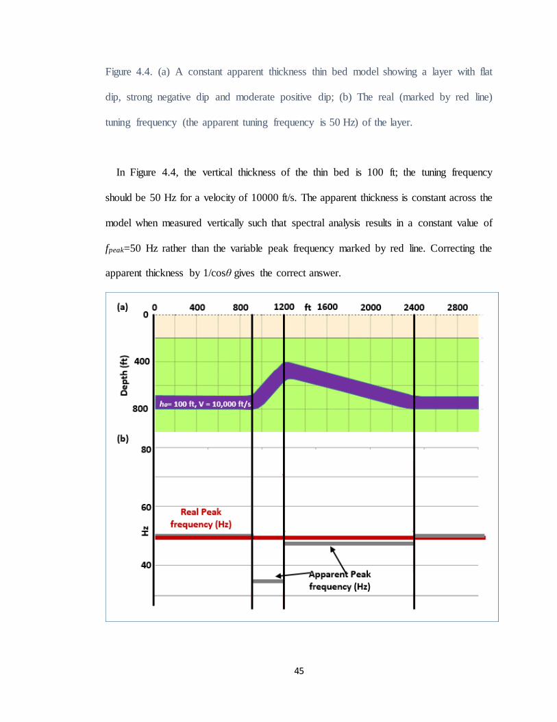
Figure 4.4. (a) A constant apparent thickness thin bed model showing a layer with flat
dip, strong negative dip and moderate positive dip; (b) The real (marked by red line)
tuning frequency (the apparent tuning frequency is 50 Hz) of the layer.
In Figure 4.4, the vertical thickness of the thin bed is 100 ft; the tuning frequency
should be 50 Hz for a velocity of 10000 ft/s. The apparent thickness is constant across the
model when measured vertically such that spectral analysis results in a constant value of
fpeak=50 Hz rather than the variable peak frequency marked by red line. Correcting the
apparent thickness by 1/cosθ gives the correct answer.

46
Figure 4.5. (a) A constant real thickness thin bed model showing a layer with flat dip,
strong negative dip and moderate positive dip; (b) The real (marked by red line) tuning
frequency (the real tuning frequency is 50 Hz) of the layer.
In Figure 4.5, the real thickness of the thin bed is 100 ft; the tuning frequency will
change the change of the vertical thickness of the thin layer. While the dip-corrected
tuning frequency of the real thickness would be constant (50 Hz) for the model.
Figure 4.6. The schematic diagram of apparent frequency (yellow line) and real frequency
(orange line).
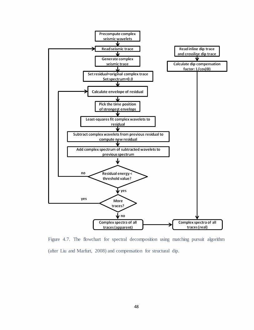
Liu and Marfurt (2008)’s matching pursuit algorithm starts by pre-computing the
wavelet dictionary. They then calculate the instantaneous envelope and frequency for
each input trace and identify key seismic events by picking a suite of envelope peaks that
fall above a user-specified percentage of the largest peak in the current (residual) trace.
They have found that this implementation converges faster and provides a more balanced
spectrum of interfering thin beds than the alternative ‘greedy’ matched pursuit

47
implementation that fits the wavelet having the largest envelope, one at a time. They
assume that the frequency of the wavelet is approximated by the instantaneous frequency
of the residual trace at the envelope peak. The amplitudes and phases of each selected
wavelet are computed together using a simple least-squares algorithm, such that the
computed amplitudes and phases result in a minimum difference between seismic trace
and matched wavelets. Each picked event has a corresponding Ricker or Morlet wavelet.
They compute the complex spectrum of the modeled trace by simply adding the complex
spectrum of each constituent wavelet. This process is repeated until the residual falls
below a desired threshold which is considered as the noise level.
48
Figure 4.7. The flowchart for spectral decomposition using matching pursuit algorithm
(after Liu and Marfurt, 2008) and compensation for structural dip.
49
Chapter 5 ATTRIBUTE ANALYSIS OF TIME- VS. DEPTH-
MIGRATED DATA
5.1. Geologic Overview
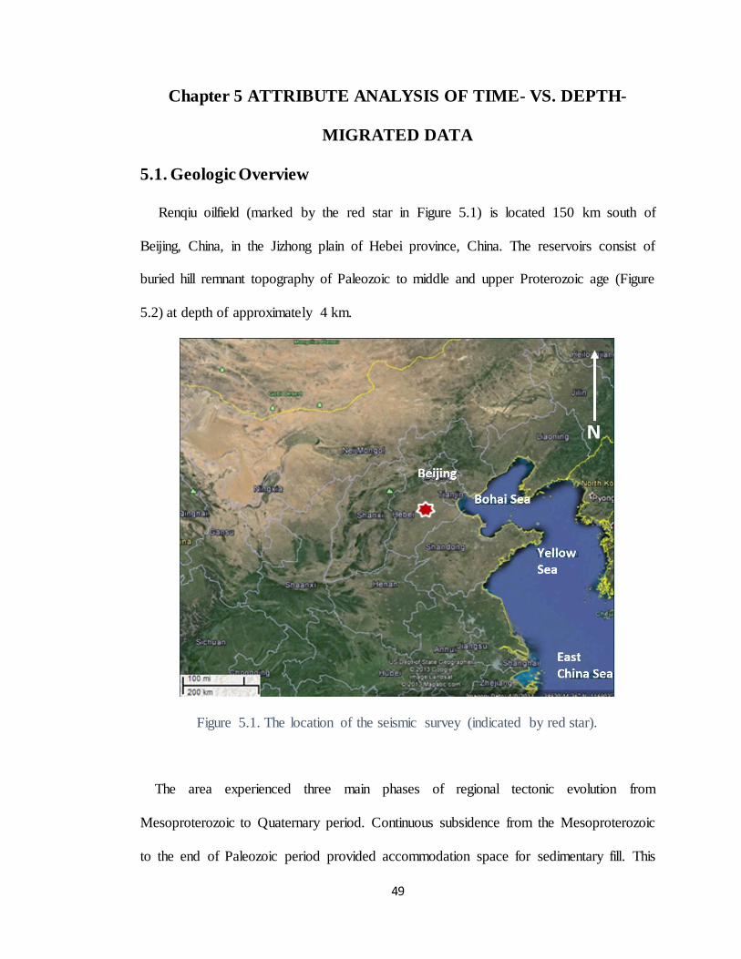
Renqiu oilfield (marked by the red star in Figure 5.1) is located 150 km south of
Beijing, China, in the Jizhong plain of Hebei province, China. The reservoirs consist of
buried hill remnant topography of Paleozoic to middle and upper Proterozoic age (Figure
5.2) at depth of approximately 4 km.
Figure 5.1. The location of the seismic survey (indicated by red star).
The area experienced three main phases of regional tectonic evolution from
Mesoproterozoic to Quaternary period. Continuous subsidence from the Mesoproterozoic
to the end of Paleozoic period provided accommodation space for sedimentary fill. This

50
was followed up warping and erosion during the Mesozoic period. Finally, there was
initiation of a rift basin from the end of the Mesozoic into the Tertiary period.
The paleo highs are remnants of the Mesozoic erosional event. The deeper underlying
carbonates were preserved and overlying Tertiary strata deposited. The continuous crustal
movement kept the basin in subsidence situation during the Tertiary period. The
maximum stratigraphic depth approaches 5500 m because of a series of extensions.
Figure 5.2. Stratigraphic column (The Eocene Epoch covered by yellow shows the main study area).
In Figure 5.3a the re-fill of the fault-controlled rift basin began with third-age of the
Himalayan movement. The sediment thicknesses vary with the width of the rift zone. In
Figure 5.3b a huge continental lake covered the basin. Lacustrine mudstone was deposited

51
during the lower and middle Es3 of Eocene Due to the quick subsidence and the warm
weather (Es3 and the following Es1 and Es2: the Eocene formations). In Figure 5.3c
fluvial facies dominated as extension decreased and was succeeded by regional uplift and
a hot dry climate. In Figure 5.3d another subsidence of the rift basin started at the end of
Es2, which exceed the lake area of the first subsidence period. The mudstone sediment
thickness was about 50 – 250 m. Finally, in Figure 5.3e at the end of the Es1, the regional
uplift began again and most of the sediments were fluvial facies with the infilling of the
lake.
Figure 5.3. The evolution of rift basin (From project report).
52
5.2. Seismic Data Quality and Conditioning
This study survey covers about 500 km2 in Hebei Province, China, including both time-
migrated data and depth-migrated data. Data were acquired and processed by BGP Inc.,
China National Petroleum Corporation. Major parameters are shown in Table 5.1.
Table 5.1. Seismic data parameters.
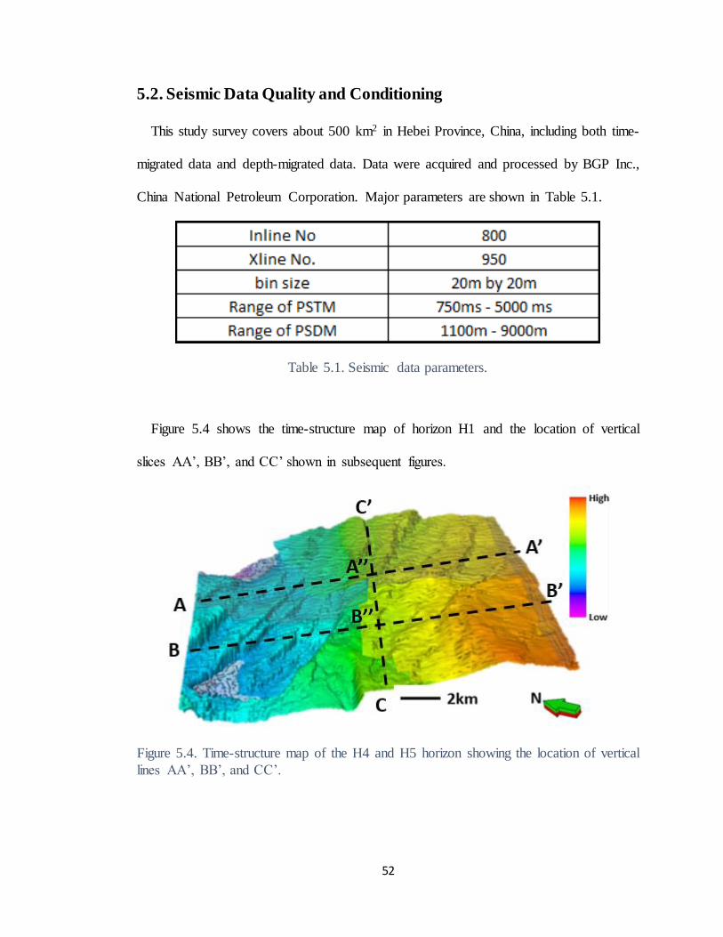
Figure 5.4 shows the time-structure map of horizon H1 and the location of vertical
slices AA’, BB’, and CC’ shown in subsequent figures.
Figure 5.4. Time-structure map of the H4 and H5 horizon showing the location of vertical
lines AA’, BB’, and CC’.

53
Figure 5.5. Time- (a) vs. depth- (b) migrated data along line AA’ (location shown in Figure 5.4). Note the clearly imaged fault-plane (F-P) reflectors indicated by the orange
arrows in (b) that helps to unambiguously link the reflector discontinuities in the shallower section. Such imaging also allows some operator aliasing noise to come into the image (red arrow). Note that in (a) the shallower and deeper reflectors indicated by
the yellow arrows are both high resolution. In contrast, the deeper event in (b) has shifted to lower wavelengths due to the increase in velocity with depth. Nevertheless, the deeper
faults indicated by the green arrow are better focused by the depth migration.

54
Figures 5.5a and b show representative vertical slices through the time– and depth–
migrated amplitude volumes. Note that the depth–migrated data has well imaged fault-
plane reflectors that cannot be seen in the time –migrated data. Unfortunately, the ability
to image such steep dips also allows steeply dipping operator aliasing to leak into the
image indicated by red arrows in Figure 5.5. The frequency resolution appears to be quite
high in both images for the shallower reflector indicated by the yellow arrows. This same
resolution appears at the deeper reflector by the yellow arrows in (a) but is lower in (b)
where the increase in velocity with depth has stretch the seismic wavelength. Most
important, the deeper faults (green arrow) are better focused in the depth migration image
which will result in more coherence anomalies.
Figure 5.6a and b show the vertical slices along line AA’’ through time- and depth-
migrated amplitude volumes. Figure 5.7a and b are the results of the Figure 5.6a and b
after the structure-oriented filtering, which improve the signal to noise ratio. Especially
for the depth-migrated amplitude volumes, the migration artifacts are suppressed very
well. However, we still have some strong artifacts indicated by blue dashed and solid
lines in Figure 5.9b. The rejected noise after structure-oriented filtering is displayed in
Figure 5.8a and b.

55
Figure 5.6. Vertical slices along line AA’’ through (a) time- and (b) depth-migrated
amplitude volumes before structure-oriented filtering). Note the erroneous apparent local
dips of the fault planes indicated by the orange arrow in the time-migrated image that are
correctly imaged in the depth-migrated image. Red arrows indicate an area of increased
noise in the depth-migrated data image. Location of line shown in Figure 5.4.
56
Figure 5.7. Vertical slices along line AA’’ through (a) time- and (b) depth-migrated
amplitude volumes after structure-oriented filtering. Note the erroneous apparent local
dips of the fault planes indicated by the orange arrow in the time-migrated image that are
correctly imaged in the depth-migrated image. The noise indicated by the red arrows was
removed or partly suppressed, compared to the one in the depth-migrated data image in
Figure 5.6. Location of line shown in Figure 5.4.

57
Figure 5.8. Vertical slices of rejected noise along line AA’’ through (a) time- and (b)
depth-migrated amplitude volumes after structure-oriented filtering. Red arrows indicate
an area of increased noise rejected after structure-oriented filtering in the depth-migrated
data image. Location of line shown in Figure 5.4.

58
Figure 5.9. Vertical slices along line AA’’ through (a) time- and (b) depth-migrated
amplitude volumes after structure-oriented filtering. Note the erroneous apparent local
dips of the fault planes indicated by the orange arrow in the time-migrated image that are
correctly imaged in the depth-migrated image. Also, note antithetic blue faults that are

59
well imaged in the depth-migrated data. Red arrows indicate an area of increased noise
in the depth-migrated data image. Location of line shown in Figure 5.4.

60
5.3. Interpretational Advantages and Disadvantages of Depth-Migrated
Data
The seismic attributes used in this chapter include curvature, coherence, volumetric dip
and azimuth, and spectral decomposition components. Curvature attributes allow one to
map both long- and short-wavelength folds and flexures. In general most-positive
curvature emphasizes the anticlinal shapes (Figure 5.10) while most-negative curvature
outlines the synclinal shapes (Figure 5.11) though both produces anomalies for bowls,
domes, and saddles. The coherence (Figure 5.13) clearly shows the distribution of faults
on time- vs. depth-migrated data. The depth-migrated data remove many artificial
structures, but also suffers from increased operator aliasing noise. Therefore, we need to
improve the data quality.

61
Figure 5.10. Vertical slice though most positive curvature co-rendered with seismic
amplitude along line AA’’ for (a) time – and (b) depth – migrated data.
Figures 5.10a and b show the vertical slices though most positive curvature co-rendered
with seismic amplitude, Figure 5.11a and b indicate the vertical slice though most
negative curvature co-rendered with seismic amplitude. The low curvature anomaly
indicated by red arrow is a syncline structure in Figure 5.11a for the time-migrated data,
while it is gone in the same location in Figure 5.11b for depth-migrated data. Orange
arrow 1 indicates a major fault we neglect in seismic amplitude profile in Figure 5.11a
and b. Orange arrow 2 shows us a more detailed structure – a minor fault in Figure 5.11b,
which does not exist in Figure 5.11a for time-migrated data.

62
Figure 5.11. Vertical slice though most negative curvature co-rendered with seismic
amplitude along line AA’’ for (a) time– and (b) depth–migrated data. Note that the most
negative curvature indicates a subtle fault (orange arrows) that was not recognized on the
earlier interpretation based only on amplitude.

63
Figure 5.12. Vertical slice though most positive curvature co-rendered with most negative
curvature (with short wavelet) and seismic amplitude along line AA’’ for (a) time – and
(b) depth – migrated data.

64
Figure 5.13. Vertical slice though most positive curvature co-rendered with most negative
curvature (with medium wavelet) and seismic amplitude along line AA’’ for (a) time –
and (b) depth – migrated data.

65
Figure 5.14. Vertical slice though most positive curvature co-rendered with most negative
curvature (with long wavelet) and seismic amplitude along line AA’’ for (a) time – and
(b) depth – migrated data.

66
Figure 5.75. Vertical slice though coherence co-rendered with seismic amplitude along
line AA’’ for (a) time – and (b) depth – migrated data. Note that the coherence indicates
a subtle fault (orange arrow) that was not recognized on the earlier interpretation based
only on amplitude.
The white arrows in Figures 5.12a, 13a and 5.14a indicate a structural high (red arrow)
and a structural low (blue arrow). In the depth-migrated data, these structural artifacts
are gone, and no high curvature value show up in the same location. A shallower velocity
67
high generates velocity pull-up in time-migrated data, while it is flat for depth-migrated
data. The blue dashed and solid lines in Figure 5.15b indicate the artifacts generated by
the pre-stack depth migration, which should be suppressed by change the migration
aperture. Unfortunately, we only have access to the stacked seismic volumes.

68
5.3.1. Coherence with Self-adaptive Window

69
Figure 5.86. Seismic profile of (a) time - and (b) depth - migrated data. (c) Depth-migrated
data with interpreted faults and horizons.
Figure 5.16 shows us vertical slices along Line AA’’ through time and depth-migrated
amplitude volumes. Orange arrows indicate faults, which are much clearer in the depth-
migrated data where many fault plane reflectors are illuminated. Red arrows indicate
migration artifacts, which are worse in the depth-migrated data than in the time-migrated
data. The reflector indicated by the yellow arrow in the depth-migrated data appears to
be a lower frequency compared to the time-migrated data. The blue arrow in depth –
migrated data shows a strong fault plane reflection, which is inaccurately imaged to a
shallower dip the in time-migrated data. The vertical apparent frequency range is 0 – 40
Hz for the time-migrated data, while the wavenumber range is about 0 – 20 cycles/km for
the depth-migrated data (Figure 5.17). Recall that migration of steep dips gives rise to
frequencies that are lower by 1/cos𝜃 of the measured frequency, and thus moves the
spectrum to fall below that of the measured (unmigrated data) spectrum. One effect of

70
depth migration is an increased steepening of the reflectors. Together with increasing
velocity, this steepening results in a greater shift to lower frequencies in the lower right
part of the image.
Figure 5.97. Smoothed (a) peak frequency of time- and (b) peak wavenumber of depth-
migrated data.

71
Figure 5.18 shows the coherence profiles computed from the time- vs. depth- migrated
data. Orange arrows indicate the three main faults, which are clearer when using the self-
adaptive window for both the time and the depth-migrated data, though stair steps still
exist. Red arrows indicate two faults. Here, the stair step phenomenon is strong in the
time-migrated data, while the faults are more continuous in the depth-migrated data. Low
coherence noise also appears to be less in the coherence profile using self-adaptive
window. The black arrows in Figures 5.18a and c show us vertical window artifacts
generated by the constant height analysis window, which are attenuated in Figures 5.18
using the self-adaptive window.

72

73
Figure 5.108. Vertical slices along Line AA’’ through coherence volumes computed from
time-migrated data using a (a) fixed height 20 ms analysis window and (b) a self-adaptive
window. Corresponding vertical slices through coherence volumes computed from depth-
migrated data using a (c) fixed height 40 ms analysis window and (d) a self-adaptive
window.

74
5.3.2. Spectral Analysis with Dip Compensation
Figures 5.19a and b indicate the peak frequency blended with seismic amplitude of
time-migrated data and depth-migrated data, respectively. Both Figures 5.19a and b
exhibit a similar peak frequency distribution, even though the values of peak frequency
in depth-migrated data is nearly half that in the time-migrated data. Low peak frequency
anomalies are lithologically bound (consistent with increasing velocity with age) along
the horizon, except for the zone seriously blurred by the migration artifacts.

75
Figure 5.119. Peak frequency co-rendered with seismic amplitude of (a) time - and (b)
depth -migrated data.
In order to describe the trend of the peak frequency, Figure 5.20a and b indicate the
peak frequency blended with seismic amplitude of the time- and depth-migrated data. The
peak frequency tracks the horizons for the time-migrated data in Figure 5.20a. The
combination of the increased velocity below the pink horizon, steeper “depth” dip than
time dip as well as some steeply dipping migration artifacts give rise to the low frequency
zones.

76
Figure 5.20. Smoothed peak frequency blended with seismic amplitude of (a) time-
migrated data and (b) depth-migrated data.
Using the algorithm described in Chapter 4, I compute dip compensation spectra and
blend the results with seismic amplitude in Figures 5.21a and b where the dip is zero
(flat), the dip compensation factor is 1.0, such that the peak frequency doesn’t change.
When there is steep dip, the dip compensation factor is greater than 1 when the horizon
has a slope, and shifts the result to a higher (true) peak frequency. The dip compensation

77
factors follow faults and horizons. Because of the greater noise in the depth-migrated
data, some of the dip estimates are erratic, giving rise to the erratic dip compensation
values shown in Figure 5.21b. Such errors can be ameliorated by first smoothing the
reflector dip estimates.
Figure 5.21. Dip compensation (1/cos𝜃) blended with seismic amplitude of (a) time - and
(b) depth - migrated data.

78
The corrected peak frequencies of time-migrated data and depth-migrated data are
displayed in Figure 5.22a and b. For the shallow part, the corrected peak frequency
changes slightly, since the dip is small and hence the dip compensation factor is close 1.
For the steeply dipping deeper layers, the corrected peak frequency is significantly
(~50%) higher than the original apparent peak frequency. Figures 5.23a and b show us
the smoothed real peak frequency of the time-migrated data and depth-migrated data. The
corrected peak frequency better correlates to the horizons than those in Figure 5.20a and
b, especially for the depth-migrated data. The low peak frequency zone (pointed by red
arrows in Figure 5.20) caused by migration artifacts in Figure 5.18b is smeared in the
vertical direction.

79
Figure 5.22. Dip corrected peak frequency co-rendered with seismic amplitude of (a) time
- and (b) depth - migrated data.

80
Figure 5.23. Smoothed (with petrel), dip-corrected peak frequency blended with seismic
amplitude of (a) time - and (b) depth - migrated data.

81
5.3.3. Seismic Interpretation
Figure 5.124 (a) Time - migrated data and time-migrated shown horizons (b) H1 (c) H2
and (d) H3.
Figure 5.24 indicates us three horizons of time-migrated data. With increased infill of
the rift basin, the reflector dip becomes progressively more horizontal such that
horizons H1 is flatter than the deeper, older horizons.

82
Figure 5.135 Time structure map of horizon H4 and H5 of the time –migrated data.
Figure 5.146 Structure map of horizon H4 and H5 of the depth – migrated data.

83
Figure 5.157 Coherence along horizon H4 and H5 of the time-migrated data.
Figure 5.168 Coherence along horizon H4 and H5 of the depth-migrated data.

84
Figure 5.179 Most positive curvature co-rendered with most negative curvature and
seismic amplitude along horizon H4 and H5 of the time-migrated data.
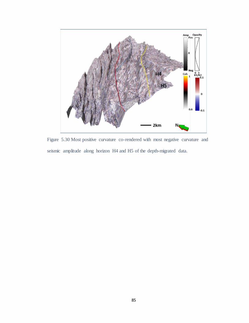
Figure 5.29 and 5.30 indicates is the most positive curvature co-rendered with most
negative curvature and seismic amplitude along horizon H4 and H5 of the time- and
depth-migrated data. The red, blue and yellow lines indicate three faults in Figure 5.29
and 5.30. The fault planes are clearer in time- than in depth-migrated data
85
Figure 5.30 Most positive curvature co-rendered with most negative curvature and
seismic amplitude along horizon H4 and H5 of the depth-migrated data.
86
Chapter 6 CONCLUSIONS
In the presence of strong lateral variations in velocity, time migration fails to image the
subsurface properly. These imaging errors can give rise to attribute artifacts. Coherence
images of fault shadows may be misinterpreted to be a second fault. Curvature anomalies
below high- or low-velocity overburden may be misinterpreted as structure. To avoid
such pitfalls, the interpreter needs to carefully calibrate the attribute anomalies to
conventional vertical slices through the seismic amplitude volume. Accurate prestack
depth migration removes most of these artifacts but introduces problems of its own. First,
fault plane reflections may be mistreated as stratigraphic reflections by most attributes.
Second, depth-migrated data are in general noisier than time-migrated data and may need
to be conditioned using structure-oriented filtering prior to attribute computation. Third,
because of the increase in velocity with depth, the corresponding change in wavelength
from top to bottom of a survey in depth-migrated data is much greater than the change in
period in time-migrated data. This longer wavelength will require different sized attribute
analysis window to maintain a similar signal-to-noise ratio.
Depth migration is designed to handle complex structure which in many cases implies
steep dips. In the presence of such steep dips one need to correct spectral estimates made
on vertical traces by 1/cos (θ) and re-interpolate the spectrum. Spectral decomposition
also provides the means to develop data-adaptive attribute analysis windows.
Specifically, I show that by defining the analysis window height to be a fraction of the
smoothed peak frequency that I can derive smoothly varying data adaptive attribute
analysis windows that maintain a similar accuracy through the seismic data volume.

87
I demonstrate the value of these modifications by applying data adaptive attribute
windows to prestack time- and depth-migrated data volumes over Renqiu Field, China.
Initially, the depth-migrated data were significantly noisier than the time-migrated data,
resulting in noisier attribute images. However, by careful structure-oriented filtering I
was able to generate superior attribute images of faulting and paleotopography that did
not suffer from the fault shadow and velocity pull-up and push-down artifacts found in
the time-migrated images.

88
REFFERENCES
Bahorich, M., A. Motsch, K. Laughlin, and G. Partyka, 2002, Amplitude responses image
reservoir: Hart’s E&P, January, 59-61.
Barnes, A. E., 2000, Weighted average seismic attributes: Geophysics, 65, 275–285.
Blumentritt, C. H., K. J. Marfurt, and E. C. Sullivan, 2006, Volume-based curvature
computations illuminate fracture orientations – Early to mid-Paleozoic, Central
Basin Platform, west Texas: Geophysics, 71, B159-B166.
Cerveny, V., and Zahradnik, J, 1975, Hilbert transform and its geophysical applications:
The Czech Digital, Acta Universitatis Carolinae. Mathematica et Physica, Vol. 16
(1975), No. 1, 67-81.
Dasgupta, S. N., J. J. Kim, A. M. al-Mousa, H. M. al-Mustafa, F. Aminzadeh, and E. V.
Lunen, 2000, From seismic character and seismic attributes to reservoir
properties: Case history in Arab-D reservoir of Saudi Arabia: 70th Annual
International Meeting, SEG, Expanded Abstract, 597-599.
Davogustto D., MC de Matos, C Cabarcas, T Dao and K. J. Marfurt, 2013, Resolving
subtle stratigraphic features using spectral ridges and phase residues:
Interpretation, 1(1), 93-108.
Fagin S., 1996, The fault shadow problem: Its nature and elimination: The Leading Edge,
1005 – 1013.
Finn, C. J., 1986, Estimation of three dimensional dip and curvature from reflection
seismic data: M.S. thesis, University of Texas, Austin.
Gersztenkorn, A., and K. J. Marfurt, 1996, Eigenstructure based coherence computations,
66th Annual International Meeting, SEG, Expanded Abstracts, 328-331.

89
Gersztenkorn, A., and K. J. Marfurt, 1999, Eigenstructure based coherence computations
as an aid to 3-D structural and stratigraphic mapping: Geophysics, 64, 1468-1479.
Hatchel, P. J., 2000, Fault whispers: Transmission distortions on prestack seismic
reflection data: Geophysics, 65, 377 – 389.
Hoecker, C., and G. Fehmers, 2002, Fast structural interpretation with structure-oriented
filtering: The Leading Edge, 21, 238-243.
Leppard, C., A. Eckersley, and S. Purves, 2010, Quantifying the temporal and spatial
extent of depositional and structural elements in 3D seismic data using spectral
decomposition and multi-attribute RGB, in L. J. Wood, T. T. Simo, and N. C.
Rosen, eds., Seismic imaging of depositional and geomorphic systems: 30th
Annual GCSSEPM Foundation Bob F. Perkins Research Conference, 1-10.
Liu, J. L., 2006, Spectral decomposition and its application in mapping stratigraphy and
hydrocarbons: PhD. Dissertation, The University of Houston.
Liu, J. L., and K. J. Marfurt, 2007, Multi-color display of spectral attributes: The Leading
Edge, 268-271.
Liu, J. L., K. J. Marfurt, and X. Guo, 2008, Instantaneous spectral attributes to detect
channels: Geophysics, 72, P23-P31.
Luo Y., S. al-Dossary, and M. Marhoon, 2002, Edge-preserving smoothing and
applications: The leading Edge, 21, 136-158.
Luo, Y., S. al-Dossary, M. Marhoon, and M. Alfaraj, 2003, Generalized Hilbert transform
and its application in geophysics: The Leading Edge, 22, 198-202.

90
Luo, Y., W. G. Higgs and W. S. Kowalik, 1996, Edge detection and stratigraphic analysis
using 3D seismic data: 66th Annual International Meeting, SEG, Expanded
Abstracts, 324 – 327.
Kuwahara, M., K. Hachimura, S. Eiho, and Kinoshita, 1976, Digital processing of
biomedical images: Plenum Press. 187-203
Marfurt, K. J., R. L. Kirlin, S. H. Farmer, and M. S. Bahorich, 1998, 3-D seismic attributes
using a running window semblance-based coherency algorithm: Geophysics, 63,
1150-1165.
Marfurt, K. J., V. Sudhakar, A. Gersztenkorn, K. D. Crawford, and S. E. Nissen, 1999,
Coherency calculations in the presence of structural dip: Geophysics, 64, 104-
111.
Marfurt, K. J., and R. L. Kirlin, 2000, 3-D broadband estimates of reflector dip and
amplitude: Geophysics, 65, 304-320.
Marfurt, K. J., 2006, Robust estimates of 3D reflector dip and azimuth: Geophysics, 71,
29-40.
Partyka, G., J. Gridley, and J. A. Lopez, 1999, Interpretational applications of spectral
decomposition in reservoir characterization: The Leading Edge, 18, 353-360.
Peyton, L., R. Bottjer, and G. Partyka, 1998, Interpretation of incised valleys using new
3D seismic techniques: A case history using spectral decomposition and
coherency: The Leading Edge, 17, 1294-1298.
Picou, C., and R. Utzmann, 1962, La coupe sismique vectorielle: Unpointe semi-
automatique: Geophysical Prospecting, 4, 497-516.

91
Puryear, C. I., S. Tai and J.P Castagna, 2008, Comparison of frequency attributes from
CWT and MPD spectral decompositions of a complex turbidities channel model:
78th Annual International Meeting, SEG, Expanded Abstracts, 393– 396.
Rietveld, W. E., J. H. Kommedal, and K. J. Marfurt, 1999, The effect of prestack depth
migration on 3D seismic attributes: Geophysics, 64, 1553-1561.
Sarkar, S., K. J. Marfurt, and R. M. Slatt, 2010, Generation of sea-level curves from
depositional pattern as seen through seismic attributes-seismic geomorphology
analysis of an MTC-rich shallow sediment column, northern Gulf of Mexico: The
Leading Edge, 29 , 1084-1091.
Singleton, S.W., M.T. Taner, and S. Treitel, 2006, Q-estimation using Gabor-Morlet joint
time-frequency analysis: 76th Annual International Meeting, SEG, Expanded
Abstracts, 1610-1614.
Taner, M. T., F. Koehler, and R. E. Sheriff, 1979, Complex seismic trace analysis:
Geophysics. 44, 1041 – 1063.
Van Bemmel, P., and R. Pepper, 2011, Seismic signal processing method and apparatus
for generating a cube of variance values: US Patent, 8, 055,026.
Widess, M. B., 1973, How thin is a thin bed? : Geophysics, 38, 1176-1254.
Young, R. A., and R. D. LoPicollo, 2005, A risk-reduction recipe using frequency-based
pore pressure predictions from seismic: Gulf Coast Association of Geological
Societies Transactions, 55, 916-921.
Zhang, K., 2010, Seismic attributes analysis of unconventional reservoirs and
stratigraphic patterns: PhD. Dissertation, The University of Oklahoma.