t -

NASA Technical Memorandum 1 0 1 5 6 4

ACOUSTIC RESPONSE OF A RECTANGULAR WAVEGUIDE WITH A STRONG TRANSVERSE TEMPERATURE GRADIENT

William E. Zorumski

( E A S d - T H - ~ O l S ~ 4 ) A C O t h l Z C BEEECLSE OF A N8E-2U I40 &fCTAbGULAB Y A V E G C I C E L I T 6 A EXEC bG IBAVSVEBSE I E E P € & A ¶ U R E G E A L f E E l ( E A S A - Langley Bcsearcb C e n t e r ) 35 F C S C L 208 Uoclas

G3/71 0; l O X 4

March 1989

National Aeronautics and Space Administration

Langley Research Center Hampton, Virginia 23665-5225

https://ntrs.nasa.gov/search.jsp?R=19890014769 2018-06-11T22:24:42+00:00Z

INTRODUCTION

The effect of temperature in acoustics is usually analyzed by allowing the speed of

sound to be a function of spatial position'*2. This type of analysis ignores the explicit

effect of the temperature gradient. It is known that the acoustic perturbation equations

contain explicit derivatives of the thermodynamic state variables, such as pressure and

density, but these derivatives may often be ignored because they are small on the scale of

an acoustic wavelength. Explicit gradient effects have been included in studies of sound

propagation in the a t r n ~ s p h e r e ~ , ~ where long wavelenghs are of interest. These wavelengths

are called infrasonic, where the temporal frequencies are on the order of 1 Hz and less.

The temperature gradient in the atmosphere is typically on the order of several kelvins

per kilometer so that the wavelength must be long in order for the temperature to vary

significantly over a wavelength. Gradient effects may be neglected in studies of audio-

frequency (20Hz-20kHz) sound in the atmosphere.

The purpose of this paper to is analyze problems whlere the temperature gradient is

strong and cannot be neglected. One problem considered is a simple rectangular cavity

with the temperature being a function of only one spatial coordinate, the one representing

the height of the cavity. This situation may occur, for example, within the structures of

high-speed aircraft where the skin is heated by a supersonic or hypersonic boundary layer.

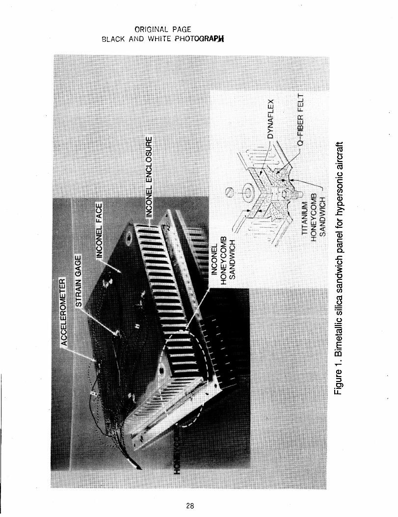
The cavity could be the interior of a Thermal Protection System (TPS)6 structural panel

such as shown in Fig. 1. The outer skin can be up to 1:350 kelvins while the inner skin

should be relatively cool, say 300 to 400 kelvins. The temperature gradient within such

a panel would then be 10 to 20 kelvins/cm, or six orders of magnitude larger than the

typical atmospheric gradient. More importantly, it is large for wavelengths of interest in

the analysis of the structural panels. The resonant frequencies of the cavity are important

parameters in the dynamic response of a panel over the cavity. If the temperature gradient,

significantly affects these resonant frequencies, then the gradient is important in predicting

the panel response. This paper will define trhe effwt, of a kmperature gradient on the

resonant frequencies of the cavity.

The panel shown in Fig. 1 is filled with insulating blankets. The acoustic properties

of such blankets may be described by the AttenboroughG model in the case of moderate

temperatures, but the inclusion of these properties would complicate the present analysis

by introducing the fibrous materials’ parameters. Also, the materials would reduce the

resonant effects studied here by way of increasing the damping of the acoustic waves.

A simpler model, shown in Fig. 2, is used here in order to focus on a single effect-

the temperature gradient. The cavity is assumed to have perfectly rigid walls with the

temperature varying linearly between the bottom and the top. A perfect gas at constant

pressure fills the cavity so that the density varies inversely with temperature.

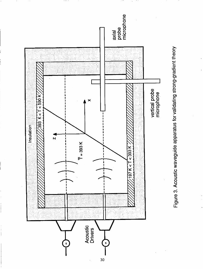
The essential features of the resonant cavity response may be verified by an experiment

on a waveguide. The waveguide, shown in Fig. 3, is like the cavity except that the width

is equal to or less than the height. The restricted width eliminates cross modes which

depend on the spatial dimension y and thus simplifies the analysis by restricting it to the

x-z plane.

A second problem where the strong gradient analysis has application is the response

of a recessed pressure sensor. Sensors are installed in recesses when the wall temperature

in high-speed boundary layer flows are above the operational limits of the pressure sensors.

When this technique is used, a transfer function must be developed to relate the sensed

pressure fluctuations to the wall pressure fluctuations. Tijdeman’~~, has given the transfer

functions in recesses where the temperature is constant. These transfer functions show

resonant peaks which depend on the cavity depth. The analysis here may be used to show

the effect of a strong temperature gradient on the transfer function for a recessed sensor.

The first section of the paper is devoted to developing the acoustic wave equation

with a temperature gradient effect. More general equations have been developed than the

one used here. Pridmore-Brown3 has given the perturbation equations including pressure,

density, and velocity gradients. Grossard and Hooke4 give completely general equations in

a rotating coordinate system to represent the earth’s atmosphere. The specialization here is

intended to emphasize a single effect. Consequently, trhe pressure is assumed to he const,ari 1,

and there is no flow. These simplifications proflii# :I \ v a l - ~ (v~iiatioii \\ Iiicli i s similar. to tlic

Helmholtz equation used in elementary acoustics. The equation is generalized, however,

by the inclusion of the temperature gradient in a coefficient. This generalized equation,

2

called the strong gradient equation, shows why the resonant frequencies of a cavity will be

altered by the gradient.

The second section of the paper is devoted to the response of a simple rectangular

cavity to a monopole source. A set of orthonormal basis functions is constructed such

that the gradient-dependent boundary conditions are satisfied. Asymptotic formulas are

derived for the effect of the temperature gradients on the modal wave numbers and phase.

The Galerkin'O method is used to express the cavity response in terms of these modes.

All integrals involved in the Galerkin procedure are evaluated by exact formulas'. Second-

order accurate asymptotic formulas are developed for the natural frequencies, modes, and

forced response of the cavity.

An experiment is suggested in the third section to verify the effects predicted here.

The experiment would use a rectangular waveguide which ia simpler than the rectangular

cavity. The width of the waveguide is selected to be small in comparison to the height so

that fewer modes will propagate. The length of the Waveguide is large in comparison to the

height. Standing waves are excited by sources at one end of the waveguide and monitored

by microphones at the other end. Temperature and temperature gradient are controlled

by heated and cooled conducting plates forming the top and bottom walls, respectively, of

the waveguide. The other sides are near-perfect insulators so that temperature variation

is one-dimensional in accordance with the theory. Excitakion frequency is varied with

excitation voltage held constant so that the microphone output represents the frequency

response function of the waveguide. Comparison of the response functions for different

combinations of plate temperature shows the temperature gradient effects. Predictions of

the resonant peaks are made to simulate the proposed experiment.

3

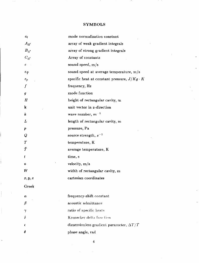
SYMBOLS

CT

C P

f 9

H

k

k

L

P

Q T T t

11

W

Greek

7

6

E

e

mode normalization constant

array of weak gradient integrals

array of strong gradient integrals

Array of constants

sound speed, m/s

sound speed at average temperature, m/s

specific heat at constant pressure, J / K g . K

frequency, Hz

mode function

height of rectangular cavity, m

unit vector in z-direction

wave number, rn-l

length of rectangular cavity, m

pressure, Pa

source strength, s-l

temperature, K

average temperature, K

time, s

velocity, m/s

width of rectangular cavity, m

Cartesian coordinates

frequency-shift constant

acoustic admittance

ratio of specific heats

Kronecker dclfa f i i i i c I ioti

dimensionless gratlieiil pa.rameter, AI’/ li’ phase angle, rad

4

W

Subscripts:

1

m

n

0

P

T 5

Y z

7 .

Special Symbols:

i f T f'

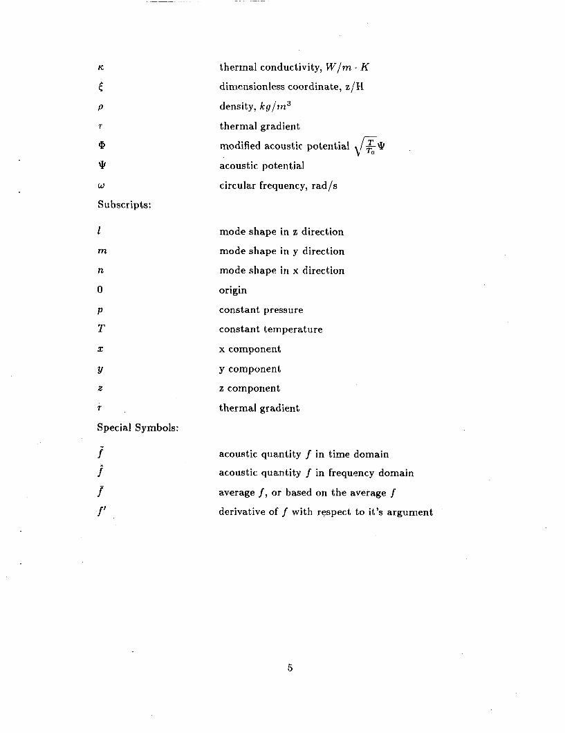
thermal conductivity, W / m K

dimensionless coordinate, z/H

density, kg / in3

thermal gradient

modified acoustic potential RQ acoustic potential

circular frequency, rad/s

t

mode shape in z direction

mode shape in y direction

mode shape in x direction

origin

constant pressure

constant temper at ure

x component

y component

z component

thermal gradient

acoustic quantity f in time domain

acoustic quantity f in frequency domain

average f, or based on the average f

derivative of f with respect to it's argument

5

STRONG T E M P E R A T U R E G R A D I E N T EFFECTS

I Acoustic Equat ions

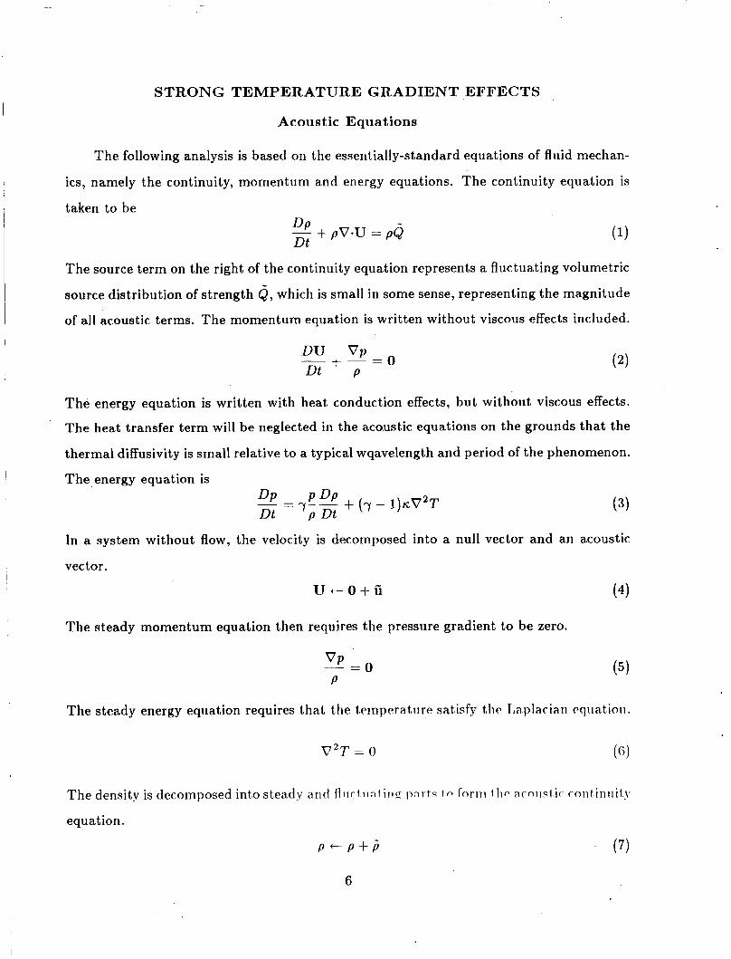
The following analysis is based on the essentially-standard equations of fluid mechan-

ics, namely the continuity, momentum and energy equations. The continuity equation is

taken to be DP Dt - + pvw = pQ

The source term on the right of the continuity equation represents a fluctuating volumetric

source distribution of strength Q, which is small in some sense, representing the magnitude

of all acoustic terms. The momentum equation is written without viscous effects included.

-

DU V p - + - = o Dt P

The energy equation is written with heat conduction effects, but without viscous effects.

The heat transfer term will be neglected in the acoustic equations on the grounds that the

thermal diffusivity is small relative to a typical wqavelength and period of the phenomenon.

The energy equation is I

DP PDP Dt p Dt - r-- + (7 -- l.)KV2T (3)

In a system without flow, the velocity is decomposed into a null vector and an acoustic

vector. I

U t O + f i (4)

The steady momentum equation then requires the pressure gradient to be zero.

VP - = o P

( 5 )

The stea.dy energy equation requires that the ternperatilre satisfy thc Laplacian t'qiiation.

The density is decomposed int,o steady a n d f l i i c f i i a i i i iE p a r t < in fnrrr i i Iic a c o i i s i ic. cont iniiit,y

equation.

P t - P + p " (7)

I 6

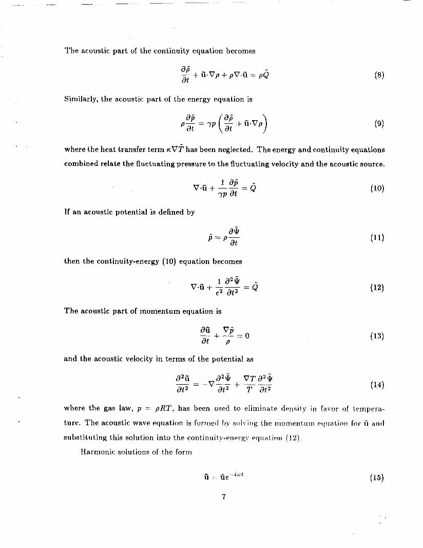
The acoustic part of the continuity equation becomes

Similarly, the acoustic part of the energy equation is

p- 86 = 7 p (g + ii.VP) at (9)

where the heat transfer term KO? has been neglected. The energy and continuity equations

combined relate the fluctuating pressure to the fluctuating velocity and the acoustic source.

If an acoustic potential is defined by

a+ f i = p - - at

then the continuity-energy (10) equation becomes

The acoustic part of momentum equation is

and the acoustic velocity in terms of the potential as

a26 VTd2\k at 2 at T at2 -- - -v--+ -- a%

(14)

where the gas law, p = pRT, has been used to eliminale density in favor of tempera-

ture. The acoustic wave equation is formed hy solving the ~no~neritutn eqiiatioii for ii and

substituting this solution into the continuity-energ! q u a t i o n ( I 2 ) .

Harmonic solutions of the form

7

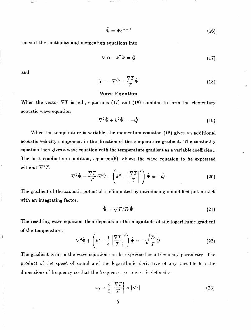
\zI $ e - ’ w t

convert the continuity and momentum equations into

~ V.G - k2$ = Q

arid A V T G

Q = - V Q + - (18) T

Wave Equation

When the vector V T is null, equations (17) and (18) combine to form the elementary

I acoustic wave equation

V2$ + k 2 $ = -Q (19)

When the temperature is variable, the momentum equation (18) gives an additional

acoustic velocity component in the direction of the temperature gradient. The continuity

equation then gives a wave equation with the temperature gradient as a variable coefficient.

The heat conduction condition, equation(6), allows the wave equation to be expressed

without V 2 T .

The gradient of the acoustic potential is eliminated by introducing a modified potential 6 I with an integrating factor.

G = d’T/To&

The resulting wave equation then depends on the magnitude of the logarithmic gradient

of the temperature.

The gradient term in the wave equation can be expressed as a frcqiicric)- paranieter. The

product of the speed of sound and the logaritlirnic tlcriwtive of a n v variaI)Ie has t h e

I dimensions of frequency so that the freqiienc\ 1);i I ,i t r i c . 1 V I i. ~ I ~ \ f i r i c ~ t l ;IS

C - w, = 2

-_ = lVCl V T T I 8

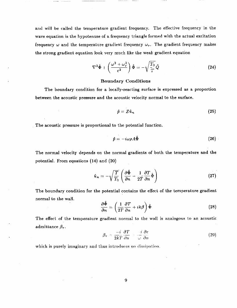
and will be called the temperature gradient frequency. The effective frequency in the

wave equation is the hypotenuse of a frequency triangle formed with the actual excitation

frequency w and the temperature gradient frequency w,. The gradient frequency makes

the strong gradient equation look very much like the weak gradient equation

Boundary Conditions

The boundary condition for a locally-reacting surface is expressed as a proportion

between the acoustic pressure and the acoustic velocity normal to the surface.

fi = 20, (25)

The acoustic pressure is proportional to the potential function.

A

fi = -iwpAQ? (26)

The normal velocity depends on the normal gradients of both the temperature and the

potential. From equations (14) and (20)

The boundary condition for the potential contains the effect

normal to the wall. - = a i ( - - + i k p ) b 1 d T d n 2T an

The effect of the temperature gradient normal to the wall

admittance pT. - i d T - i d c

__ - - - pr = 2kTiG LL' a??

(27)

of the temperature gradient

(28)

is analogous to an acoustic

(29)

which is purely imaginary and thus introdirces J ~ O tlissipa t inti.

9

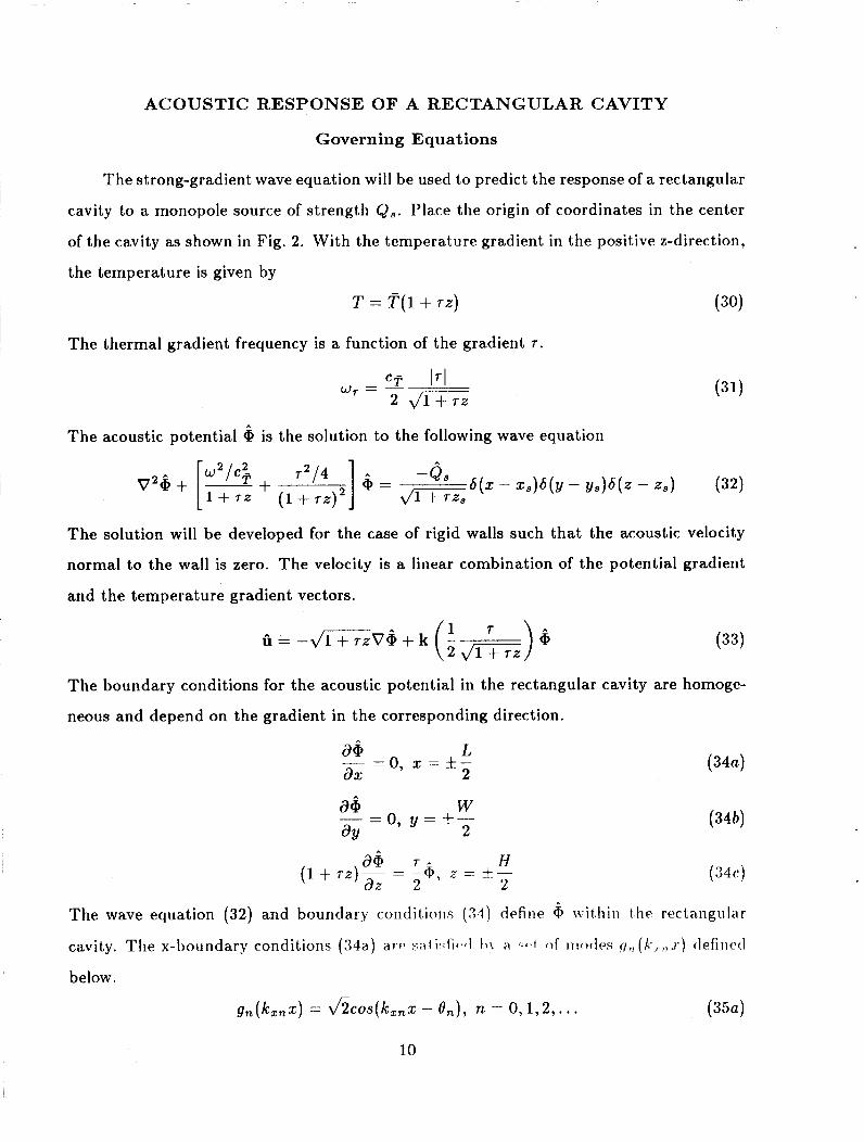
ACOUSTIC RESPONSE OF A R E C T A N G U L A R CAVITY

Governing Equations

The strong-gradient wave equation will be used to predict the response of a rectangular

cavity to a monopole source of strength Q 3 . Place the origin of coordinates in the center

of the cavity as shown in Fig. 2. With the temperature gradient in the positive z-direction,

the temperature is given by

T = T(1+ T Z ) (30)

The thermal gradient frequency is a function of the gradient r .

CT 171

2 4n-E 0, = -

The acoustic potential 6 is the solution to the following wave equation

The solution will be developed for the case of rigid walls such that the acoustic velocity

normal to the wall is zero. The velocity is a linear combination of the potential gradient

and the temperature gradient vectors.

The boundary conditions for the acoustic potential in the rectangular cavity are homoge-

neous and depend on the gradient in the corresponding

L - = o , z = f- a i d X 2

W - = o , y = f - a6 aY 2

direction.

86 T - H (1 + 72)-- = - @ , 2 = +-

a z 2 2 ( 3 4 4

The wave equation (32) and boundary conditions (34) define Q, w i t l i i i i the rectangular

cavity. The x-boundary conditions ( M a ) arc’ < a t i r : f i < \ ( l I ? I i> c - * % f o f iiio(1w !I,, ( k , . , , . r ) tlefinetl

below.

gn(/c,,z) = ~ 5 c o s ( 1 ~ ~ , s - dn), n = 0 , 1 , 2 , . . . ( 3 5 4

10

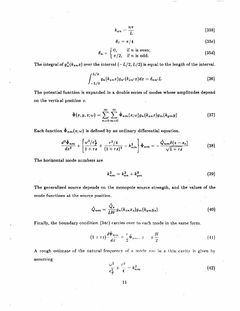
0, if n is even; d n = { 7r/2, if n is odd. ( 3 5 4

The integral of g;(kznz) over the interval ( - L / 2 , L / 2 ) is equal to the length of the interval.

The potential function is expanded in a double series of modes whose amplitudes depend

on the vertical position z.

n = O m=O

Each function &am(*; w ) is defined by an ordinary differential equation.

The horizontal mode numbers are

(39) 2 k:m = k2, + k,,

The generalized source depends on the monopole source strength, and the values of the

mode functions at the source position.

Q S Qnm = - gn (kznzs) gm (kymys) LW

Finally, the boundary condition (34c) carries over to each inode in the same form.

A rough estimate of the natural frequency of a 111orle 7 7 m in a t h in cavit,;v is given hy

assuming

11

This simple estimate indicates that the natural frequency will be less than the natural

frequency = cpknm of a cavity without a temperature gradient.

The effect of the gradient-dependent boundary conditions on the acoustic modes is devel-

oped in the following section.

Basis Functions

Basis functions in the vertical dimension are generalizations of the cosine functions in

the horizontal dimensions.

g l (kz l z ) = alcos(k*lz - 621) ( 4 4 )

These functions must satisfy boundary conditions which depend on the temperature gra-

dient.

The boundary conditions yield the following characteristic equation for the wave number

kzr .

( 4 6 )

(47)

2 € 2 (4 - c ~ ) ~ : ~ H ~ + c 2

- - tan kz lH kZlH

c = r H = A T / p

The series for tan x/x contains only even powers so that ( k z l H ) 2 is a function of (AT/p)2.

The branch is selected such that the two variables have the same sign when they are real-

valued. The series also provide asymptotic formulas for the wave numbers. ,

The lowest order wave number is proportional to the t<eiiiperat tire gradient,, l)uk t,he higher-

order wave numbers are functions of the square of t81ie teniperaturc gradicnl.

The phase of the modes is found from c ~ i i l i ~ ~ t l ~ ~ ~ i i t i ~ l ; i i \ ( ) t ) d i 1 i t ) t i .

( 2 f E)k,1Hsin k , l H / 2 f E C O S k , l H / 2 ( 2 f E)k,l Hcos k,l H f 2 f csin k,l H f 2

tan 6,1 = f ( 4 9 )

12

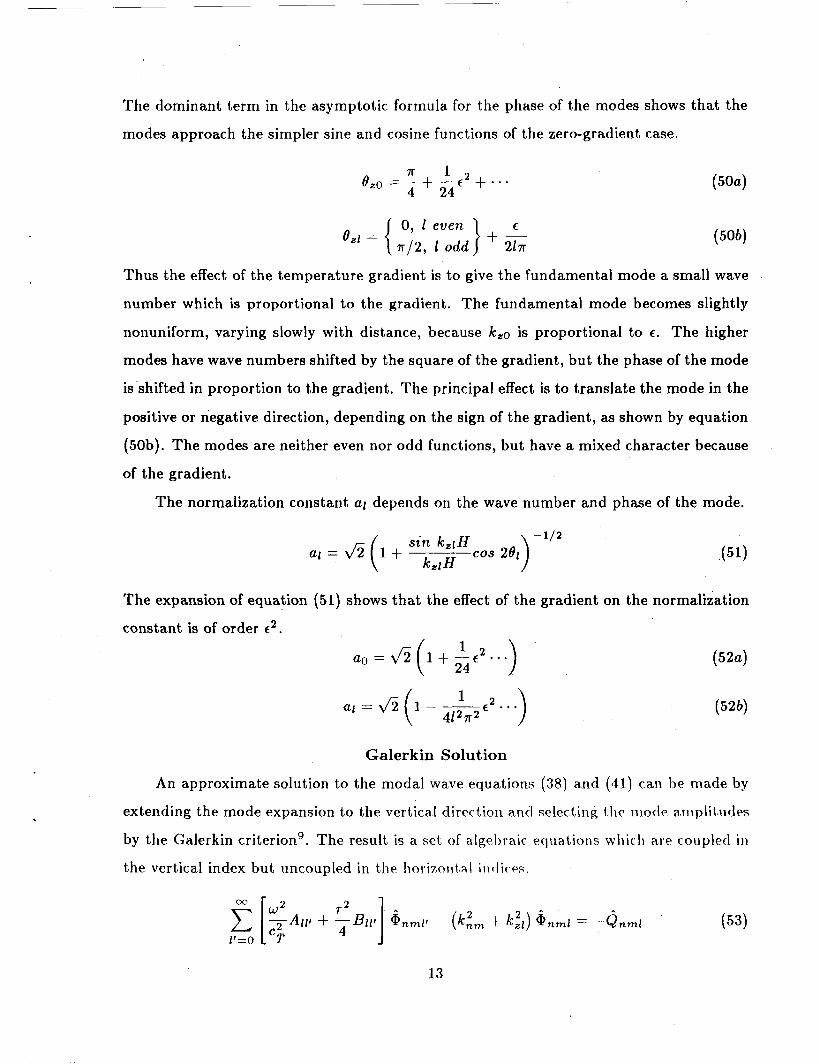
The dominant term in the asymptotic formula for the phase of the modes shows that the

modes approach the simpler sine and cosine functions of the zero-gradient case.

0, 1 even €

Thus the effect of the temperature gradient is to give the fundamental mode a small wave

number which is proportional to the gradient. The fundamental mode becomes slightly

nonuniform, varying slowly with distance, because k,o is proportional to e . The higher

modes have wave numbers shifted by the square of the gradient, but the phase of the mode

is shifted in proportion to the gradient. The principal effect is to translate the mode in the

positive or negative direction, depending on the sign of the gradient, as shown by equation

(sob). The modes are neither even nor odd functions, but have a mixed character because

of the gradient.

The normalization constant a1 depends on the wave number and phase of the mode.

sin k,lH cos 2e1

The expansion of equation (51) shows that the effect of thte gradient on the normalization

constant is of order e'.

Galerkin Solution

An approximate solution to the modal wave equations (38) and ( 4 1 ) can be made by

extending the mode expansion to the vertical direct ion and selecting the mode amplitudes

by the Galerkin criteriong. The result is a set of algebraic equations wliicli are coupled ill

the vertical index but uncoupled in the hor ixon t a1 i i idkw.

13

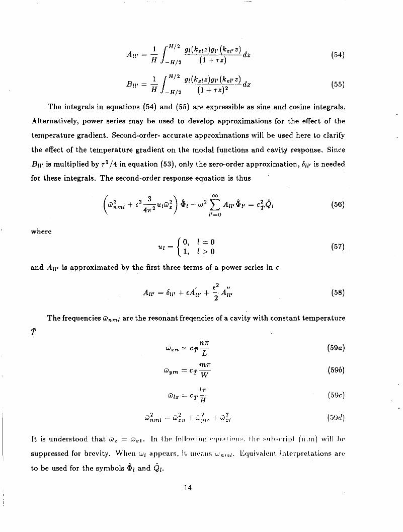
The integrals in equations (54) and ( 5 5 ) are expressible as sine and cosine integrals.

Alternatively, power series may be used to develop approximations for the effect of the

temperature gradient. Second-order- accurate approximations will be used here to clarify

the effect of the temperature gradient on the modal functions and cavity response. Since

B1p is multiplied by r2/4 in equation (53), only the zero-order approximation, 611, is needed

for these integrals. The second-order response equation is thus

where 0, l = O 1, l > O u1= {

and Alp is approximated by the first three terms of a power series in e

(57)

The frequencies Unml are the resonant freqencies of a cavity with constant temperature

T

It is understood that = W,l . In t h e f o l l o n ~ i t i c ~ ~ ~ 1 i i q > 1 i c r r i ~ . . tlic sril>sc-ril)f ( i i . i r i ) will I ) ?

suppressed for brevity. When c i ~ l appears, i t , t i i w i i s LI,,,,~. kkluivalent, inkrprelations arc

to be used for the symbols &[ and Q I .

14

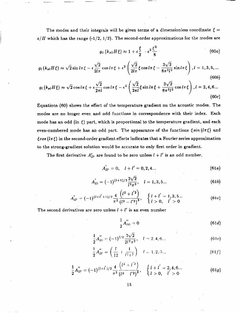
The modes and their integrals will be given terms of a dimensionless coordinate ( =

z / H which has the range (-l/2, l/2). The second-order approximations for the modes are

(604

Equations (60) shows the effect of the temperature gradient on the acoustic modes. The

modes are no longer even and odd functions in correspondence with their index. Each

mode has an odd (in E ) part, which is proportional to the temperature gradient, and each

even-numbered mode has an odd part. The appearance of the functions ( s in( ln[) and

tcos (1.0 in the second-order gradient effects indicates that a Fourier series approximation

to the strong-gradient solution would be accurate to only first order in gradient.

The first derivative Aill are found to be zero unless 1 + 1' is an odd number.

1 + 1' = 1,3,5 ... ( 1 + 1 ) + 1 ) / 2 4 ( 1 2 + 1 ' 2 ) A;, = (-1)

( 1 2 - 1 ' 2 ) 2 ' 1 > 0, I t > 0

The second derivatives are zero unless 1 + I' is an even number

15

Natural Frequencies and Modes

Homogeneous solutions of equations (56) are possible at resonant frequencies wl which

depend on the temperature gradient parameter c. These resonant frequencies are solutions

of the infinite determinant equation

IwaA1p - bill (a; + E ~ s ~ u : ) ~ = O (62)

When this determinant is expanded, it is found that the cofactor of any element of order

6 is also of order E. Consequently, the resonant frequencies are functions of E’ and can be

approximated as

w; w (2; (1 + €2.1) (63)

The corresponding natural modes, designated by xlr are given as

Since the homogeneous solution (64) may be multiplied by an arbitrary constant, there

is no loss of generality in taking xi:’ = 1 , xi:) = 0 and xi,?’ = 0. The remaining elements

of the vectors are found by substituting the assumed solution (64) with the series (58 ) for

Alp into the homogeneous equation from (56) and collecting coefficients of each power of

c. The zero order vectors are the Kronecker delta function

The first order vectors are proportional to the first derivatives All’

where D[ is the reduced frequency for the mode

m H

The second-order vectors are found to depend 011 l , l it . second derivative ,4;;, and o n prodric1,s

of the first derivatives.

16

where

j # l ’

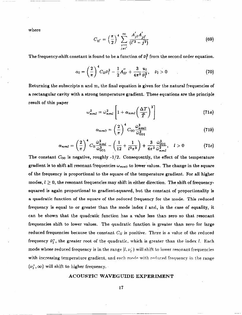
The frequency-shift constant is found to be a function of i i f froin the second order equation.

4

i j l > o 1 ‘ I

al = ( f ) C~D,? - - A l I j + -- 2 4764 ti?’

Returning the subscripts n and m, the final equation is given for the natural frequencies of

a rectangular cavity with a strong temperature gradient. These equations are the principle

result of this Daper

The constant Coo is negative, roughly -1/2. Consequently, the effect of the temperature

gradient is to shift all resonant frequencies WmnO to lower values. The change in the square

of the frequency is proportional to the square of the temperature gradient. For all higher

modes, 1 2 0, the resonant frequencies may shift in either direction. The shift of frequency-

squared is again proportional to gradient-squared, but the constant of proportionality is

a quadratic function of the square of the reduced frequency for the mode. This reduced

frequency is equal to or greater than the mode index 1 and, in the case of equality, it

can be shown that the quadratic function has a value less than zero so that resonant

frequencies shift to lower values. The quadratic function is greater than zero for large

reduced frequencies because the constant C ~ I is positive. There is a value of the reduced

frequency DT, the greater root of the quadratic, which is greater than t8he index 1 . Each

mode whose reduced frequency is in the range [ I , vi) will shift to lower resonant frequencies

with increasing temperature gradient, and each nincle with retliiced frequency in the range

(v;, 00) will shift to higher frequency.

ACOUSTIC WAVEGUIDE EXPERIMENT

17

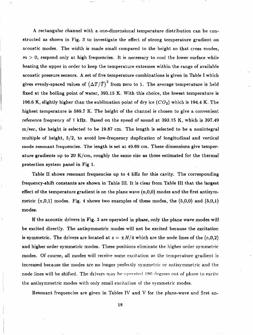
A rectangular channel with a one-dimensional temperature distribution can be con-

structed as shown in Fig. 3 to investigate the effect of strong temperature gradient on I

acoustic modes. The width is made small compared to the height so that cross modes,

rn > 0, respond only at high frequencies. It is necessary to cool the lower surface while

heating the upper in order to keep the temperature extremes within the range of available

acoustic pressure sensors. A set of five temperature combinations is given in Table I which

gives evenly-spaced values of (AT/F)2 from zero to 1. The average temperature is held

fixed at the boiling point of water, 393.15 K. With this choice, the lowest temperature is

196.6 K, slightly higher than the sublimation point of dry ice ((702) which is 194.4 K. The

highest temperature is 589.7 K. The height of the channel is chosen to give a convenient

reference frequency of 1 kHz. Based on the speed of sound at 393.15 K, which is 397.49

I m/sec, the height is selected to be 19.87 cm. The length is selected to be a nonintegral

multiple of height, 5/2, to avoid low-frequency duplication of longitudinal and vertical

mode resonant frequencies. The length is set at 49.69 cm. These dimensions give temper-

ature gradients up to 20 K/cm, roughly the same size as those estimated for the thermal

protection system panel in Fig 1. I

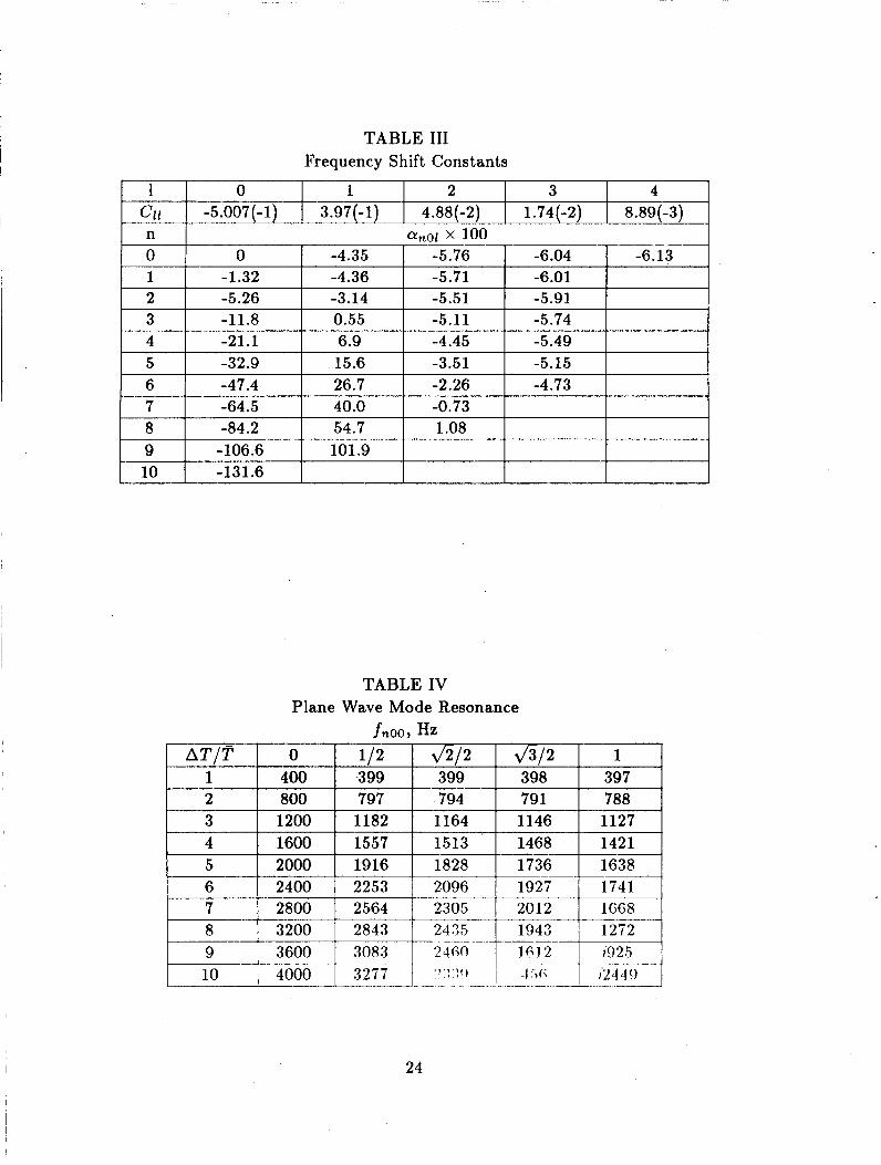
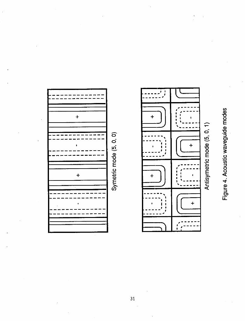
Table I1 shows resonant frequencies up to 4 kHz for this cavity. The corresponding

frequency-shift constants are shown in Table 111. It is clear from Table 111 that the largest I , I I

effect of the temperature gradient is on the plane wave (n,O,O) modes and the first antisym-

metric (n,O,l) modes. Fig. 4 shows two examples of these modes, the (5,0,0) and (5,0,1)

modes. I

If the acoustic drivers in Fig. 3 are operated in phase, only the plane wave modes will

be excited directly. The antisymmetric modes will not be excited because the excitation

l is symmetric. The drivers are located at z = f H / 4 which are the node lines of the (n,0,2)

and higher order symmetric modes. These positions eliminate the higher order symmetric

modes. Of course, all modes will receive some excitation as the temperature gradient is

increased because the modes are no longer perfectly symmetric or antisymmetric and the

node lines will be shifted. The drivers may he n p e i ~ t ~ 4 180 clqrees oilf of phase to excite

the antisymmetric modes with only small excitation of the symmetric modes.

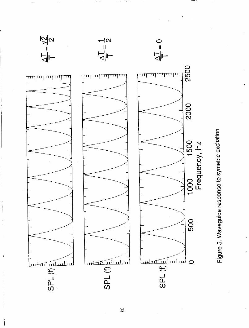
Resonant frequencies are given in Tables IV and V for the plane-wave and first an-

18

tisymmetric modes, respectively. The (10,0,0) mode has imaginary frequencies in the

extreme case where AT/F = 1, but this is outside the limit where the asymptotic theory

is valid. In any event, the tendency of increasing gradient should be to decrease the reso-

nant frequencies of the plane-wave modes so the waveguide response should be as shown

in Fig. 5 with symmetric excitation. With no temperature gradient, there should be 6

resonant peaks between 0 and 2.5 kHz. When the temperature gradient is increased to

AT/T = 1/2, the lower resonant peaks should be unaffected, but there should be a percep-

tible downshift of the 4th, 5th and 6th peaks. When the temperature gradient is increased

to &/2 there should be a more pronounced shift and a 7th peak should appear.

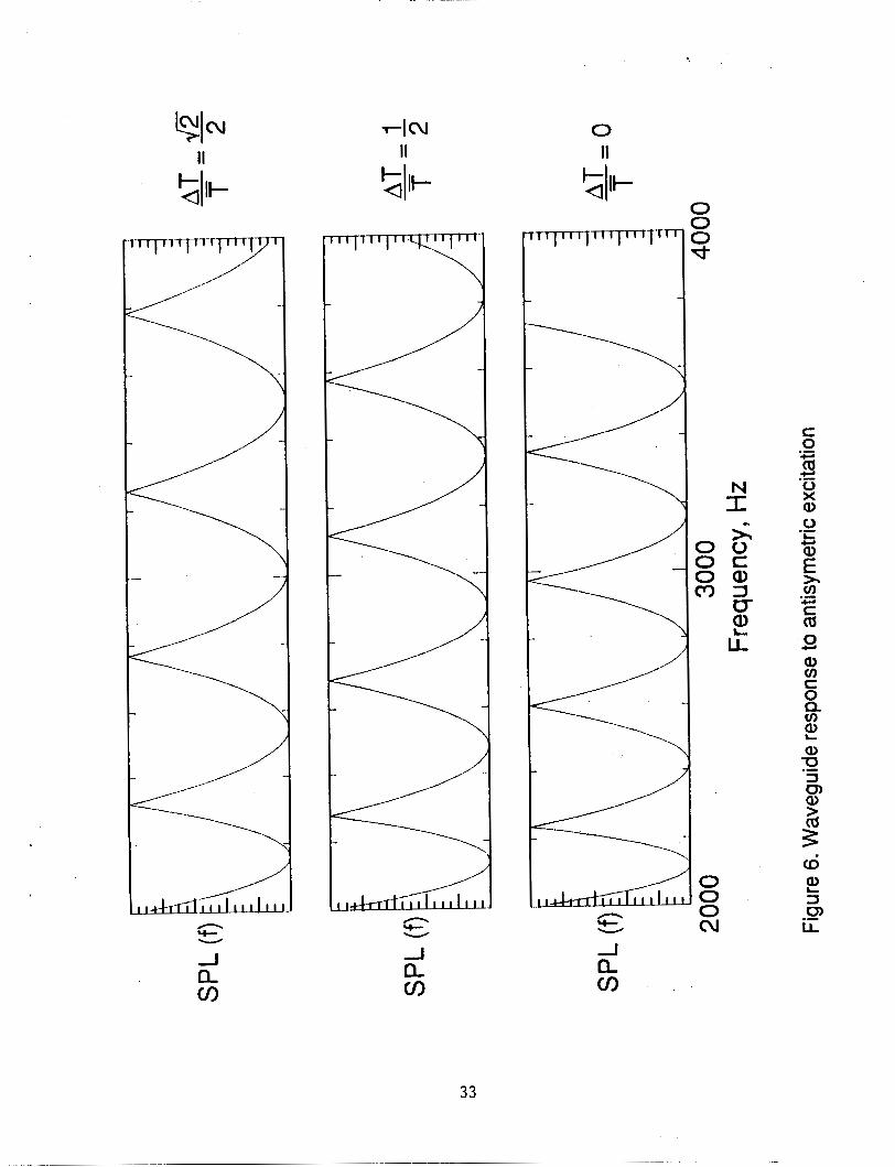
Fig. 6 shows the anticipated response of a waveguide to antisymmetric excitation. The

response is shown from 2 to 4.4 kHz because the resonant frequencies should shift upward

in this range. Without a temperature gradient, ther are five resonant peaks, the lowest at

2236 Hz and the highest at 3736 Hz. As the temperature gradient, is increased to .\/i/2,

the lowest peak should shift upward by about 100 Hz and the highest should shift up by

over 600 Hz.

19

CONCLUDING REMARKS

Temperature gradients is gases affect acoustic waves by way of a spatially-variable

sound speed. In general, the sound speed and its derivatives appear in the wave equation

in a function which is a variable coefficient of the acoustic potential. When the gradients

are small, the derivatives can be neglected and the function depends only on the speed of

sound. This approximation has been called the weak gradient theory in this paper. There

are problems where the gradients are not small, (on the scale of a typical wavelength)

and a modified wave equation has been developed here for these cases. This modified

equation has been called a strong gradient wave equation. The essential modification

is the addition of the square of the sound speed gradient to the square of the circular

frequency. The acoustic boundary conditions are altered by adding a negative imaginary

admittance p r to the wall. The magnitude of this admittance is the ratio of the normal

I

I

derivative of the sound speed to the circular frequency. I The strong gradient theory has been applied to determine the resonant frequencies of

rectangular cavities with temperature gradients in the direction of a one coordinate. It

has been shown that the resonant frequencies of the cavity are changed in proportion to

the square of the temperature gradient. Asymptotic formulas, accurate to second order in

the temperature gradient, have been developed for the resonant frequencies and normal

modes of the cavity.

These formulas show that the modes with small variation in the gradient direction will

all shift to lower resonant frequencies. Higher modes, both symmetric and antisymmetric

in the gradient direction, may shift to lower or to higher resonant frequencies, depending

on their zero gradient frequency.

A conceptual experiment has been defined to study the effects of gradients on reso-

nant frequencies. The experiment uses a two-dimensional waveguide roughly 20 cm high

by 50 cm long to study the frequency range from 400 Hz to 4 k H z . The average tem-

perature in the waveguide is held fixed at about the boiling point of water, 393 K while

varying the temperature of the upper and Ion~~~i 911 t faces of the wal.pguide. Heating the

upper surface while cooling the lower produces a thermally-stable stratification of air wi th

a nearly-constant temperature gradient. Symmetric excitation of the waveguide should

20

excite longitudinal, nearly-plane, modes whose resonant frequencies will shift downward

with increasing temperature gradient. Antisymmetric excitation may be used to excite

longitudinal modes whose frequencies should shift upward with increasing gradient. This

experiment will provide a critical test of the strong gradient theory.

21

REFERENCES

1. Pekeris, C. L.: Theory of Propagation of Sound in a Half-space of Variable Sound

Velocity under Conditions of Formation of a Shadow Zone. J. Acoust. SOC. Amer., Vol.

18, No. 2, October, 1946. pp. 295-315.

2. Brekhovskikh, L. M.: Waves in Layered Media. Second Edition Translated by Robert

T. Beyer. Academic Press, 1980.

3. Pridmore-Brown, David C.: Sound Propagation in a Temperature- and Wind-Stratified

Medium. J. Acoust. SOC. Amer. Vol. 34, No. 4, April 1962. pp. 438-443.

4. Grossard, Earl E.; and Hooke, William H.: Waves in the Atmosphere. Atmospheric

Infrasound and Gravity Waves - their Generation and Propagation. Elsevier Scientific

Publishing Company, 1975.

5 . Blair, Winford: Manufacturing Experiences for Advanced Multiwall Prepackaged

Metallic TPS. Advances in TPS and Structures for Space Transportation Systems. NASA

Conference Publication 2315, Decenber 1983. pp. 261-302.

6. Attenborough, Keith: Acoustic Characteristics of Rigid Absorbents and Granular

Materials. J. Acoust. SOC. Amer., vol. 73, No. 3, March 1983. pp. 785-799.

7. Tijdeman, H.: Investigations of the transonic flow around oscillating airfoils. NLR-

TR-7709O-U, Oct. 21, 1977.

8. Tijdeman, H.: On the Propagation of Sound Waves in Cylindrical Tubes. Journal of

Sound and Vibration, vol. 39, 1975, pp. 1-33

9. Finlayson, Bruce A.: The Method of Weighted Residuals and Variational Principles

with Application in Fluid Mechanics, Heat and Mass Transfer. Academic Press, Inc. 1972.

Gradshteyn, I. S.; and Ryzhik, I. M.: Table of Intrgrals, Series, and Products. 10.

Translation edited by Alan Jeffrey. Academic Press, 1965.

22

A T / F Tl T2

AT, K TI, K/cm

TABLE I1 Waveguide Natural Frequencies

L=49.69 cm, H=19.87cm, T=393.:15 K n/l 0 1 2 0 0 1000 2000 3000

0 112 393.2 294.9 254.2 196.6 393.2 491.4 532.1 563.4 589.7

0 196.6 278.0 393.2 0 11.80 14.14 17.32 20.00

1 400 1077 2040 2 800 1281 2154

23

AT/T 1

I I I I I I Cll I -5.007(-1) I 3.97(-1) I 4.88(-2) 1 1.74(-2) [ 8.89(-3)

0 112 w d 3 / 2 1 400 399 399 398 397

2 3 4 5

800 797 794 79 1 788 1200 1182 1164 1146 1127 1600 1557 1513 1468 1421 2000 1916 1828 1736 1638

6 7 8

24

2400 2253 2096 1927 1741 2800 2564 2305 2012 lG68 3200 2843 2435 1943 1272

TART,E V First Antisymmetric Mode Resonance

fnOl, HZ

3 4 5 6 7 8

1000 978 956 932 909 1077 1071 1065 1059 1053 1281 1276 1271 1266 1261 1562 1563 1564 1565 1566 1887 1889 1890 1892 1893 2236 2279 2322 2363 2404 2600 2685 2 768 2848 2927 2973 3118 3257 3390 3518 3353 3575 3784 3982 4170

I I I I 1

9 I 3736 1 4063 I 4365 1 4648 I 4914

25

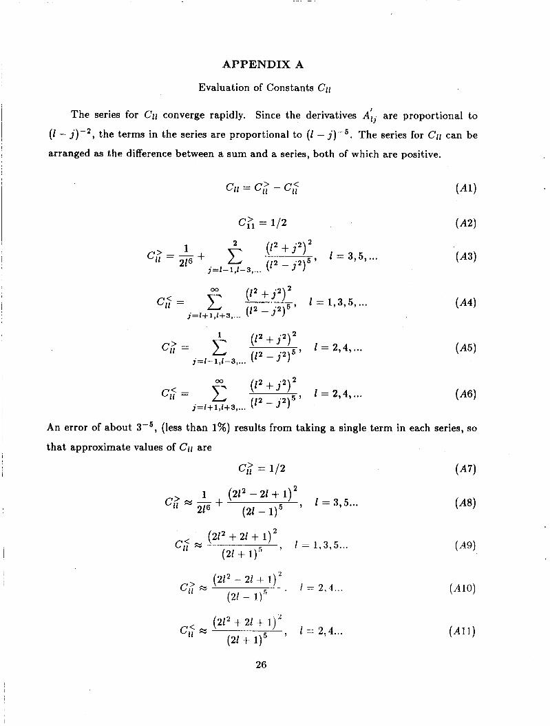
APPENDIX A

Evaluation of Constants Cll

The series for CII converge rapidly. Since the derivatives Aij are proportional to

(1 - j ) - 2 , the terms in the series are proportional to ( I - j ) - 6 . The series for Cl1 can be

arranged as the difference between a sum and a series, both of which are positive.

c,>, = 112

1 = 3,5, ... 1 (12 + j 2 ) 2 c;=-+ (12 - j 2 ) 5 ’

216 j = l - 1, l -3 ,...

1 = 2,4, ... j = l + 1,1+3 ,...

An error of about 3-‘, (less than 1%) results from taking a single term in each series, so

that approximate values of C ~ I are

c; = 1/2 (A7)

1 (212 - 21 + 1)2

c; R3 , 1 = 1 , 3 , 5 ...

, 1 = 3 , 5 ... ci+s+ (21 - q5 (212 + 21 + 1)2

(21 + q5 (212 - 21 + 1y

(21 - 1 y c; M -. I = 2 , 4 ...

(212 + 21 + l j Z c; M , 1 = 2 , 4 ... (21 + q5

26

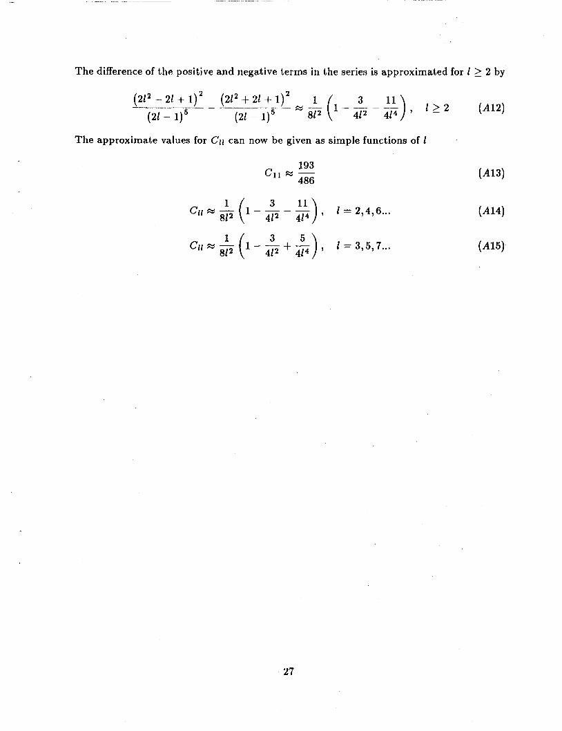
The difference of the positive and negative terms in the series is approximated for 1 2 2 by

The approximate values for CII can now be given as simple functions of 1

193 C11% -

486

1 = 2,4,6 ...

CII M - 1 = 3 , 5 , 7 ...

27

ORIGINAL PAGE BLACK AND WHITE PHOTWRAPJrf

28

X

l- a

h

cl N -

\ \

+- t a, U cd .-

0 c

v) 2 c,

a

3 r, .-

.- E.

8 >

29

30

I I +

I

-7)

e - - - - - .

IC e-----.

'------

E e - - - - - (

I I I-----

31

-1 0

32

3 3 3

N I s

0 0 o r o a m 3 CT a IL

0 0 0 cv

33

Report Documentation Page

I

4. Title and Subtitle

Acoust ic Response o f a Rectangular Waveguide w i t h a Strong Transverse Temperature Gradient

7. Author(s)

Wi l l i am E. Zorumski

9. Performing Organization Name and Address

Langley Research Center Hampton, V i r g i n i a 23665-5225

12. Sponsoring Agency Name and Address

1. Report No. 1 2. Government Accession No. I 3. Recipient's Catalog No.

5. Report Date

March 1989 6. Performing Organization Code

8. Performing Organization Report No.

10. Work Unit No.

505-61-11-01 11. Contract or Grant No.

13. Type of Report and Period Covered

I NASA TM- 101564 I

19. Security Classif. (of this report) 20. Security Classif. (of this page) 21. No. of pages

Uncl ass i f i ed U n c l a s s i f i e d 34

22. Price

A0 3

Nat ional Aeronaut ics and Space Admin i s t ra t i on Washington, DC 20546-0001

I

15. Supplementary Notes

Presented a t t he A I A A 27th Aerospace Sciences Meeting i n Reno, Nevada January 9-12, 1989.

16. Abstract

An acous t ic wave equat ion i s developed f o r a p e r f e c t gas w i t h s p a t i a l l y - v a r i a b l e temperature. The s t rong-grad ien t wave equat ion i s used t o analyze t h e response o f a rec tangu lar waveguide con ta in ing a t h e r m a l l y - s t r a t i f i e d gas. It i s assumed t h a t t h e temperature g rad ien t i s constant, represent ing one-dimensional heat t r a n s f e r w i t h a constant c o e f f i c i e n t of c o n d u c t i v i t y . The ana lys i s o f t h e waveguide shows t h a t t he resonant f requencies o f t h e waveguide a r e s h i f t e d away from the values t h a t would be expected from the average temperature o f t he waveguide. For small g rad ien ts , t h e frequency s h i f t i s p ropor t i ona l t o t h e square o f t he grad ien t . of the na tu ra l frequency of t h e waveguide w i t h un i fo rm temperature. An exper i - ment i s designed t o v e r i f y t h e essen t ia l features o f t h e s t rong-grad ien t theory .

The f a c t o r o f p r o p o r t i o n a l i t y i s a quadra t i c f u n c t i o n

17. Key Words (Suggested by Authods)) I 18. Distribution Statement

Acoust ic Waves Sound Speed Gradient Temperature Gradient Acoust ic Resonance

U n c l a s s i f i e d - Un l im i ted Subject Category 7 1