ORIGINAL INNOVATION Open Access

Across-fault ground motions and theireffects on some bridges in the 1999 Chi-Chi earthquakeYuanzheng Lin1,2, Zhouhong Zong1,2*, Jin Lin1,2, Yale Li3 and Yiyan Chen4

* Correspondence: zongzh@seu.edu.cn1Engineering Research Center ofSafety and Protection of Explosion& Impact of Ministry of Education(ERCSPEIME), Southeast University,Nanjing 211189, Jiangsu, China2School of Civil Engineering,Southeast University, Nanjing211189, Jiangsu, ChinaFull list of author information isavailable at the end of the article

Abstract

Simply-supported bridges are vulnerable to surface fault rupture as evidenced byseveral fault-crossing bridges in the 1999 Chi-Chi earthquake. To investigate theseismic collapse mechanism of simply-supported bridges crossing the fault, across-fault ground motions are firstly simulated in the present study. In particular, basedon a previously developed fault model of the 1999 Chi-Chi earthquake, broadbandacross-fault ground motions at six fault-crossing bridges are simulated using thehybrid deterministic-stochastic method, in which the low- and high-frequencycomponents are computed using the deterministic Green’s function method and thestochastic finite-fault modeling method, respectively. The simulation results indicatethat the hybrid deterministic-stochastic method can give reasonable predictions tothe across-fault ground motions. Furthermore, utilizing the explicit dynamic finiteelement (FE) code LS-DYNA, behaviors of a three-span simply-supported bridgeunder a selected pair of across-fault ground motions are numerically simulated.Numerical results indicate that the structural responses and collapse mechanisms aredominated by the low-frequency ground motions. The large differential static offsetacross the fault is the main reason for the collapse of the simply-supported bridges.This study contributes understandings for the across-fault ground motions and thecollapse mechanism of some bridges in the 1999 Chi-Chi earthquake.

Keywords: Across-fault ground motion, Ground motion simulation, Simply-supported bridge, Seismic collapse analysis, Explicit dynamic FE model, Chi-Chiearthquake

1 IntroductionOn 21 September 1999, a devastating earthquake of Mw 7.6 occurred in central

Taiwan. The epicenter was located at 120.82°E, 23.85°N, with a focal depth of 8 km,

and the mainshock ruptured over 100 km along the Chelungpu fault with a shallow dip

angle of about 30° to the east (Shin and Teng 2001). After the earthquake, extensive

studies were performed to investigate the focal mechanism, rupture process and fault

slip history (Chi et al. 2001; Ji et al. 2003; Ma et al. 2001; Wu et al. 2001). This earth-

quake caused significant damages to vital infrastructures including transportation brid-

ges, roads, utilities and communication lines (Lee and Loh 2000). In particular, the

© The Author(s). 2021 Open Access This article is licensed under a Creative Commons Attribution 4.0 International License, whichpermits use, sharing, adaptation, distribution and reproduction in any medium or format, as long as you give appropriate credit to theoriginal author(s) and the source, provide a link to the Creative Commons licence, and indicate if changes were made. The images orother third party material in this article are included in the article's Creative Commons licence, unless indicated otherwise in a creditline to the material. If material is not included in the article's Creative Commons licence and your intended use is not permitted bystatutory regulation or exceeds the permitted use, you will need to obtain permission directly from the copyright holder. To view acopy of this licence, visit http://creativecommons.org/licenses/by/4.0/.

Advances inBridge Engineering

Lin et al. Advances in Bridge Engineering (2021) 2:8 https://doi.org/10.1186/s43251-020-00028-1

surface fault rupture passed through seven highway bridges located along the

Chelungpu fault. With either the main structure or the approach road traversed by sur-

face fault rupture, these bridges suffered serious damages. For example, Fig. 1a shows

the girder unseating of the Bei-Feng Bridge due to the large ground displacement in-

duced by fault dislocation; Fig. 1b shows the collapse of the Tong-Tou Bridge due to

the shear failure of the piers; Fig. 1c shows the severe shear failures in the columns and

caissons of the Wu-Shi bridge though the bridge did not collapse (Lee and Loh 2000;

NCREE 2002). In addition to these cases, damages of fault-crossing bridges were re-

peatedly reported in the past earthquakes, e.g. the 1999 Kocaeli and Duzce earthquakes

in Turkey, and the 2008 Wenchuan earthquake in China (Han et al. 2009; Kawashima

et al. 2009; Yang and Mavroeidis 2018). Although the construction of a bridge crossing

a fault should be avoided from the design point of view, it is difficult to avoid existing

bridges to be traversed by potential active faults due to the complexity and uncertainty

of earthquake faults, especially in seismic prone areas.

Damages of fault-crossing bridges are related to the nonuniform ground movements

across the fault. Somerville (2002) concluded that the displacements across a fault are

discontinuous, which can subject a bridge to significant differential displacements in-

cluding both quasi-static displacements and dynamic motions between the bridge sup-

ports located on two sides of the fault. Over the years, forward modeling of strong

ground motion has achieved considerable progress (Papageorgiou 2003). In particular,

the hybrid deterministic-stochastic method, which combines the low-frequency and

high-frequency ground motions computed by the deterministic method and stochastic

approach respectively (Kamae et al. 1998), has been widely adopted and proven to show

reasonable predictions to the near-fault ground motions (e.g. Ding et al. 2019). How-

ever, not many studies have adopted this technique to simulate across-fault ground mo-

tions. Because the across-fault ground motions are a pair of near-fault ground motions

with the two very close observation points locating on two sides of the fault, the hybrid

deterministic-stochastic method is believed applicable to simulate across-fault ground

motions as well. It should be mentioned that some other approaches have been devel-

oped to simulate across-fault ground motion recently. For example, across-fault ground

motion can be obtained by combining the parametrically determined low-frequency

pulse component and the high-frequency component of a strong-motion record (e.g.

Yang et al. 2020; Zhang et al. 2020). Due to the assumption that the ground dislocation

is distributed equally among the two sides of the fault, this method only applies to

strike-slip fault scenario and cannot be used in dip-slip fault scenario. As a different

method, the improved empirical baseline correction approach based on the target final

displacement also can be used to simulate the across-fault ground motions (Lin et al.

Fig. 1 Damage cases of the fault-crossing bridges in the 1999 Chi-Chi earthquake: a unseating of the Bei-Feng Bridge; b collapse of the Tong-Tou Bridge; c shear failure of the Wu-Shi Bridge

Lin et al. Advances in Bridge Engineering (2021) 2:8 Page 2 of 21

2018, 2020a, b, 2021). However, this method requires real across-fault ground motion

records that are actually very rare and limited, which therefore confines the application.

Because the hybrid deterministic-stochastic method is based on the earthquake source

model, the above limitations can be avoided. It is necessary to use this method to simu-

late across-fault ground motions considering its potentional benefits for seismic per-

formance analysis of the bridges crossing fault-rupture zones.

Some research efforts were made on the seismic behavior of bridges crossing fault-

rupture zones. Goel and Chopra (2009a, b) proposed linear and nonlinear analysis

methods based on structural dynamics. Saiidi et al. (2013) conducted a shake table test

of a two-span girder bridge crossing strike-slip fault-rupture zones. Anastasopoulos

et al. (2008) proposed a methodology for the design of bridges against tectonic deform-

ation. The Bolu Viaduct, which was traversed by the surface rupture and suffered se-

vere damage, has been widely investigated as it survived in the 1999 Duzce, Turkey

earthquake (Pamuk et al. 2005; Park et al. 2004; Roussis et al. 2003; Ucak et al. 2014).

Hui (2015) did extensive investigations on the ground motion inputs, the bridge re-

sponses and the coping strategies against the effect of surface faulting. These studies

primarily focused on the influence of strike-slip faults, while the responses of bridges

traversed by dip-slip faults have not been sufficiently investigated (Lin et al. 2020a). It

should be mentioned that different fault mechanisms can induce very different ground

movements across the fault. For a strike-slip fault, the two rock blocks on the two sides

of the fault move horizontally and slide past one another, which induces a reversed

ground motion waveform in the fault-parallel direction but the same ground motion in

the fault-normal direction on two sides of the fault. For a dip-slip fault, the two rock

blocks on the two sides of the fault move downward or upward relative to each other

with a dip angle to the horizontal ground surface. Depending on the fault geometry

and slip properties, the across-fault ground motions of a dip-slip fault are much more

complicated compared to those of a strike-slip fault (Lin et al. 2020a). Therefore, it is

imperative to investigate the bridge seismic behaviors with the considerations of cross-

ing dip-slip faults.

This paper presents a comprehensive study on the simulations of across-fault ground

motions and the seismic collapse analyses of the fault-crossing bridges in the 1999 Chi-

Chi earthquake. Following the fault model developed by Wu et al. (2001), the low- and

high-frequency ground motions are computed using the deterministic Green’s function

method and the stochastic finite-fault modeling method respectively, and they are then

combined into broadband across-fault ground motions and validated against the

ground motion prediction equations (GMPEs). Furthermore, using explicit finite elem-

ent (FE) code LS-DYNA, a case study of a typical simply-supported bridge is performed

to investigate its seismic responses and collapse mechanism subjected to the across-

fault ground motions.

2 Simulation of across-fault ground motions2.1 Fault model

Extensive studies have been carried out to investigate the fault rupture process and slip

distribution of the 1999 Chi-Chi earthquake, and many fault models have been devel-

oped which are useful for further analyses (Chi et al. 2001; Ji et al. 2003; Ma et al. 2001;

Lin et al. Advances in Bridge Engineering (2021) 2:8 Page 3 of 21

Wu et al. 2001). In the present study, the finite-source rupture model developed by Wu

et al. (2001) is utilized to further simulate the across-fault ground motions. In particu-

lar, the entire fault plane is assumed as a rectangle with the dimensions of 84 × 44 km

(length × width) and is then discretized at a grid interval of 1 km with 3696 pieces of

subfaults. On the ground surface, the fault plane has a trace with a strike of N5°E and a

dip angle of 30°. Figure 2 shows the detailed geometry of the fault model. Through an

inversion using strong-motion data from 47 stations and global positioning system

(GPS) data from 60 GPS stations, the fault rupture process including the slip, rake

angle and rupture time of each subfault are obtained (Wu et al. 2001). Figure 2 also

presents the slip distribution of the entire fault plane. It can be seen that the large slip

occurs mainly in the shallow section of the faulting area in the northern part with the

largest slip over 20 m. The inversion results indicated that the reverse component is

dominant in most of the faulting area, while the rupture propagates to the deep north-

ern part with strike-slip and dip-slip components. Besides, long rise time and large slip

are two significant features of the Chi-Chi earthquake from the inversion results (Wu

et al. 2001). It should be mentioned that this fault model is obtained from the Finite-

Source Rupture Model Database (Mai 2015), which is the simplest one (i.e. Model A)

of the three models developed by Wu et al. (2001).

In this study, the aforementioned fault slip model is used to simulate the across-fault

ground motions based on the hybrid deterministic-stochastic method. Because the

across-fault ground motions are predicted based on the fault model by using this

method, some low-frequency features incorporated in velocity pulse and permanent

ground displacement at a specific site, which is strongly related to its local fault slip

properties, can be accurately predicted. In addition, the discontinuity of the displace-

ment across the fault at a specific site can also be reasonably predicted. The accurate

prediction of fault dislocation features in the across-fault ground motions is a major ad-

vantage of this method compared to the other methods of ground motion simulation.

However, this method requires detailed information of a fault model including geom-

etry properties, slip distribution, risetime, rupture process and plenty of computational

Fig. 2 Fault slip model developed by Wu et al. (2001)

Lin et al. Advances in Bridge Engineering (2021) 2:8 Page 4 of 21

parameters, and thus it may only be used based on a well-known or validated fault

model.

2.2 Fault-crossing bridges and observation locations

As mentioned in many earthquake reconnaissance reports for the 1999 Chi-Chi earth-

quake (e.g. Lee and Loh 2000; NCREE 2002), there were seven bridges traversed by the

surface fault rupture. These bridges were all small or middle span simply-supported

bridges, and they were constructed by T-shaped beams, single-column or thin-wall

piers and elastomeric bearing pads. The damage modes of these bridges included

unseating of the superstructure, shear failure and tilting of the piers and complete col-

lapse of the structure. In particular, the unseating of the superstructure is very common

and has been a major concern for the simply-supported bridges. Table 1 summarizes

the locations, span arrangements and damage modes of these fault-crossing bridges.

These fault-crossing bridges are sequentially marked along the surface rupture as

shown in Fig. 3a. Among them, six bridges (Site 2 to 7) located along the main rupture

trace, while the Shi-Wei Bridge (Site 1) located at a secondary rupture segment bending

towards the east. Along the surface fault rupture, the epicenter located between the

Ming-Tsu Bridge and the Bauweishan Viaduct. Except for the Shi-Wei Bridge, the rest

six bridges distributed along the main rupture of the fault. Figure 3b shows the bridge

locations (except for the Shi-Wei Bridge) along the assumed surface rupture for ground

motion simulations, namely the assumed observation points. In particular, the locations

along the surface rupture are calculated by the GPS coordinates as shown in Table 1.

In the perpendicular direction of the surface rupture, the distance from the observation

points to the surface rupture is set as 500 m (see Fig. 3b). It should be noted that for

fault-crossing bridges, the bridge supports on the two sides of the fault may be very

close to the surface rupture. However, a very small fault distance may induce abnormal

results for the low-frequency ground motions using the deterministic Green’s function

method. The reason is that Green’s functions use r−4, r−2, and r−1 forms for the near-,

intermediate-, and far-field terms respectively, where r is the distance from the

Table 1 Details of the fault-crossing bridges in the 1999 Chi-Chi earthquake

Site Bridge GPS location Spanarrangement

Damage description

1 Shi-Wei Bridge 120.797°E,24.285°N

3 × 25m Unseating of two spans, shear failure of piers,tilting of abutments

2 Bei-Feng Bridge 120.760°E,24.280°N

13 × 30 m Unseating of three spans, pier collapse

3 E-Jian Bridge 120.734°E,24.133°N

24 × 12 m Unseating of 12 spans, pier collapse

4 Wu-Shi Bridge 120.670°E,24.008°N

18 × 34.8 m Unseating of two spans, shear failure of piers

5 BauweishanViaduct(underconstruction)

120.706°E,23.902°N

– Shear failure of foundations, pounding damageof abutments, tilting of piers

6 Ming-Tsu Bridge 120.707°E,23.816°N

28 × 25 m Unseating of nine spans, shear failure of piers,tilting of piers

7 Tong-Tou Bridge 120.658°E,23.651°N

4 × 40m Complete collapse

Lin et al. Advances in Bridge Engineering (2021) 2:8 Page 5 of 21

observation point to the surface rupture, and thus the traction Greens’ functions will

peak very sharply for a very small r (Spudich and Archuleta 1987). The fault distance of

500 m is believed a reasonable value that is enough close to the surface rupture for

simulating the ground movements while avoiding the above computational issues.

2.3 Low-frequency ground motion

The low-frequency component of earthquake ground motion is deterministic, which

can be simulated or predicted by using a theoretical seismology model. In seismology,

the deterministic method is based on the elastodynamic representation theorem pro-

posed by Burridge and Knopoff (1964) and further developed by Aki and Richards

(1980). According to this theory, the ground motion at an observation point can be

computed by a spatial and temporal convolution of the Green’s function with the fault

slip function, which is given by

un x; tð Þ ¼Z ∞

− ∞dτ∬ΣΔui ξ; τð Þcijpqv j ∂

∂ξqGnp x; t; ξ; τð ÞdΣ ξð Þ ð1Þ

where cijpq is the elasticity tensor, v is a unit vector normal to the fault, Δui(ξ, τ) is the

i-th component of the slip on the fault, and Gnp(x, t − τ; ξ, 0) is the Green’s function

representing the n-th component of the synthetic displacement at the observation point

when an impulsive source in the p-th direction is applied at x = ξ and t = τ.

In the present study, Green’s functions for wave propagation are computed using the

discrete wavenumber representation method (Bouchon 1979; Bouchon and Aki 1977;

Olson et al. 1984). This method includes the complete response of the earth structure

Fig. 3 Plan view of the fault-crossing bridges in the 1999 Chi-Chi earthquake: a real bridge locations; bobservation points for ground motion simulation. The red lines indicate the surface fault rupture; the redstar indicates the epicenter; the dashed rectangle indicates the projection of the fault model on the groundsurface; and the upward and downward triangles represent the simulation locations on the hanging-walland footwall sides, respectively

Lin et al. Advances in Bridge Engineering (2021) 2:8 Page 6 of 21

so that all the P and S waves, surface waves and near-field terms are considered. This

method has been used by many researchers and proven yielding good predictions to

the low-frequency near-fault ground motions (e.g. Ding et al. 2019; Wu et al. 2001). In

the present study, a horizontally layered velocity structure is assumed, which is tabu-

lated in Table 2. This layered velocity structure model is obtained from the Finite-

Source Rupture Model Database (Mai 2015) and is slightly different from the models

provided by Wu et al. (2001) It should be mentioned that no special efforts are made

to compare the results using different layered velocity structure models, nevertheless,

this model is believed reasonable to predict ground motions.

For a finite-source rupture model, the slip on a subfault is time-dependent and can

be characterized by rupture onset time, slip rate and slip duration (i.e. risetime). The

fault slip function can be given by

Δui ξ; tð Þ ¼ Δui ξð Þs t; ξð Þ ð2Þ

where Δui(ξ) is the final slip, and s(t, ξ) is the slip rate and risetime function. In the

present study, a boxcar function is adopted as the fault slip rate-time function, which is

shown in Fig. 4. The boxcar function has a simple form and can achieve permanent dis-

placement due to its asymmetric form. When the fault rupture arrives at a given sub-

fault, the corresponding slip at the subfault occurs. The slip trigger time of each

subfault depends on the rupture propagation process. Previous studies concluded that

the rupture velocity varies from 1.6 to 4.0 km/s in different regions of the fault plane

with an average value of about 2.5 km/s (Chi et al. 2001; Ji et al. 2003; Ma et al. 2001;

Wu et al. 2001). In this study, a constant rupture velocity of 2.5 km/s is assumed and

used to determine the rupture onset time of each subfault. In addition to the Green’s

function and the fault slip function, some other parameters are properly selected for

simulating the ground motions. In particular, the maximum frequency for computing

Green’s functions is set as 1.0 Hz, the seismic moment is set as 2.7 × 1020 N·m accord-

ing to the solution from Wu et al. (2001) and the duration of the simulated ground mo-

tions is set as 90 s.

Figure 5 shows the simulation results of the low-frequency across-fault ground mo-

tions at each bridge site. For a straightforward demonstration, the across-fault ground

motions have been processed using a low-pass filter with the cut-off frequency of 0.50

Table 2 Layered velocity structures

Depth (km) Vp (km/s) Vs (km/s) Density (t/m3)

0.00 2.88 1.55 2.00

0.91 3.15 1.70 2.05

1.91 4.37 2.50 2.30

3.70 5.13 2.85 2.40

8.00 5.90 3.30 2.60

13.00 6.21 3.61 2.70

17.00 6.41 3.71 2.75

25.00 6.83 3.95 2.80

30.00 7.29 4.21 3.00

35.00 7.77 4.49 3.10

50.00 8.05 4.68 3.10

Lin et al. Advances in Bridge Engineering (2021) 2:8 Page 7 of 21

Hz. It can be seen from Fig. 5 that the simulated low-frequency ground motions are very

different along the main fault rupture (from Site 2 to 7). In particular, the simulated

ground motions in the northern regions (e.g. Site 2) shows larger peak ground accelera-

tions (PGAs), peak ground velocities (PGVs) and peak ground displacements (PGDs) than

those in the southern regions (e.g. Site 7), which can be explained by the following two

reasons. The main reason is that the low-frequency ground motions at these observation

points are mainly dominated by the fling-steps, which are related to the local fault slip as

shown in Fig. 2, in which the fault slip increases gradually from south to north. The other

reason is that the epicenter located in the southern region, and with the fault breaking

from south to north, forward directivity effect occurs when the rupture propagates to the

northern regions, which further enhances the pulse components. It is also noted in Fig. 5

that the ground motions on the two sides of the fault are significantly different at a spe-

cific site. In particular, the ground motions on the hanging-wall side show larger inten-

sities compared to the corresponding ground motions on the footwall side due to the

hanging-wall effect. In addition, the permanent ground displacements on the hanging-

wall side are also significantly larger than the corresponding components on the footwall

side, implying the ground movements mainly occur on the hanging-wall, moving upwards

relative to the footwall. Different permanent ground displacements on the two sides of the

fault induce significant differential displacements across the fault. For example, the

ground motions at the Bei-Feng Bridge (No. 2) show permanent differential displacements

of 5.7 m, 3.4 m and 7.4m in the vertical, fault-parallel and fault-normal directions respect-

ively, which can be very dangerous for the fault-crossing bridges.

2.4 High-frequency and broadband ground motions

The high-frequency component of the ground motion is fundamentally different from

the low-frequency component, showing strong stochastic behavior, which is random

and difficult to be depicted by the theoretical seismology model. In the present study,

the high-frequency ground motions are simulated based on the stochastic method de-

scribed by Boore (1983, 2003) In this method, the primary consideration is to deter-

mine the spectrum of the ground motion, which can be given by

Y M0;R; fð Þ ¼ E M0; fð ÞP R; fð ÞG fð ÞI fð Þ ð3Þ

where M0 is the seismic moment; E(M0, f) is the source spectrum function, and its

amplitude can be determined by M0; P(R, f) represents the path effect function that ac-

counts for the geometrical spreading, attenuation, and the general increase of duration

with distance due to wave propagation and scattering; G(f) is the local site effect func-

tion, which is used to consider the amplification due to local site geology and the at-

tenuation due to path-independent loss of energy; I(f) is an operator determining the

Fig. 4 Slip rate-time function: a slip rate; b slip. The risetime is the duration from t1 to t2

Lin et al. Advances in Bridge Engineering (2021) 2:8 Page 8 of 21

type of the output ground motion (i.e. acceleration, velocity or displacement output).

This method is also referred to as the stochastic point-source method.

In a large earthquake, the source properties including fault geometry, slip distribution

and directivity, etc., can significantly influence the ground motion at the observation

point near the fault. To incorporate these factors, a large fault can be divided into N

Fig. 5 Simulation results of the low-frequency ground motion time histories at each bridge site: aacceleration; b velocity; c displacement. The number of each subplot indicates the peak value with the unitin cm/s2, cm/s and cm for acceleration, velocity and displacement, respectively. The numbers on the leftcorrespond to the bridges listed in Table 1

Lin et al. Advances in Bridge Engineering (2021) 2:8 Page 9 of 21

pieces of subfaults with each one considered as a small point source. The rupture

spreads radially from the hypocenter and triggers slips on subfaults sequentially. The

ground motions induced by each subfault is calculated by the stochastic point-source

method, and these ground motions are summed with a proper time delay to obtain the

ground motion for the entire fault (Motazedian and Atkinson 2005), which can be

given by

a tð Þ ¼XNl

i¼1

XNw

j¼1

aij t þ Δtij� �

ð4Þ

where Nl and Nw represent the number of the subfaults along the length and width of

the fault plane, respectively (Nl ×Nw =N); Δtij is the relative delay time for the radiated

wave from the ij-th subfault to reach the observation point; aij is the ground motion at

the observation point due to each subfault, which is calculated by the stochastic point-

source method. This stochastic finite-fault modeling technique has been a useful tool

for the prediction of near-fault ground motions of a large earthquake. In the present

study, the high-frequency ground motions are simulated using the source-based sto-

chastic finite-fault code EXSIM developed by Motazedian and Atkinson (2005) This

computer code has been widely used to predict the near-fault ground motions with fair

accuracy in the high-frequency range (e.g. Sun et al. 2015).

Some studies have been performed to predict the ground motions in the 1999 Chi-

Chi earthquake using the stochastic finite-fault modeling method (e.g. D’Amico et al.

2012; Lekshmy and Raghukanth 2019; Liu et al. 2012; Roumelioti and Beresnev 2003).

In the present study, the fault model for computing high-frequency ground motion is

consistent with that used in the low-frequency ground motion simulation as demon-

strated in Section 2.1. The modeling parameters used in EXSIM are mainly from

D’Amico et al. (2012) as tabulated in Table 3. In particular, the parameters regarding

the crustal properties, attenuation and geometric spreading, etc., have been validated

against the observation results. The crustal amplification is considered using the

NEHRP site class C (Vs30 = 520 m/s) as given by Boore et al. (1997).

It should be mentioned that the EXSIM program is primarily developed to simulate

the horizontal earthquake ground motions, with no special intention for the vertical

ground motions. In the present study, the vertical ground motions are obtained

through scaling the horizontal ground motions by an empirical vertical to horizontal

(V/H) ratio of 0.64. This scale factor is determined by the average V/H ratios of 130

strong-motion records from the 1999 Chi-Chi earthquake (Wang et al. 2002). It should

be noted that this simplified approach to obtain the vertical ground motions has no sig-

nificant influence on the simulation results.

The broadband across-fault ground motions are obtained by combining the corre-

sponding low- and high-frequency ground motions in the time domain, and a matched

low- and high-pass filters at the cut-off frequency of 0.50 Hz is used. Figure 6 shows

the broadband across-fault ground motions at the selected six bridge sites. It can be

seen that the simulated broadband across-fault ground motions are very different on

the two sides of the fault. In particular, the PGAs on the hanging-wall side are on aver-

age 24% larger than those on the footwall side due to the hanging-wall effect. In

addition, while the across-fault ground motions at different sites along the fault rupture

Lin et al. Advances in Bridge Engineering (2021) 2:8 Page 10 of 21

show varying PGAs, the northern observation points generally show greater PGAs than

those in the southern areas. The reason is that very large slips occur in the northern

areas (see Fig. 2), where the effect of forward directivity is also more prominent com-

pared to the southern areas. It also can be observed from Fig. 6 that the broadband

across-fault ground motions exhibit some differences in the PGVs and PGDs when

compared to the corresponding low-frequency ground motions as shown in Fig. 5.

However, the waveforms of the velocity pulses are not significantly affected and the dis-

placement time histories are almost unchanged, implying the velocity and displacement

time histories of the across-fault ground motions are primarily dominated by the low-

frequency components.

It should be mentioned that as observed in Section 2.3, differential displacements

exist across the fault, which is also incorporated in the broadband across-fault ground

motions. Thus, for the thrust fault considered in this study, the hanging-wall effect and

the permanent differential displacements across the fault are two main characteristics

of the across-fault ground motions, which may have significant impacts on the fault-

crossing bridges. As will be presented in Section 3, simply supported bridges can be

very vulnerable and may suffer structural collapse due to surface faulting movements.

2.5 Comparison to ground-motion prediction equations

Since there are hardly any available ground motion records at or very close to the fault-

crossing bridges, the simulated across-fault ground motions are compared to the

GMPEs. In the present study, the GMPE proposed by Abrahamson et al. (2014), namely

ASK14, is used for comparison. In particular, ASK14 allows the regionalization of Vs30

scaling and the anelastic attenuation for Taiwan, and also considers the scaling for the

Table 3 Modeling parameters for the 1999 Chi-Chi earthquake in EXSIM

Parameter Value

Moment magnitude 7.6

Stress drop Δσ (bar) 90

Kappa (s) 0.05

Fault orientation (strike/dip) 5°/30°

Fault dimensions (length × width) 84 km × 44 km

Subfault dimensions 1 km × 1 km

Slip distribution Wu et al. (2001)

Crustal shear-wave velocity (km/s) 3.2

Crustal density (g/cm3) 2.8

Rupture to shear-wave velocity ratio 0.8

Anelastic attenuation, Q(f) 350(f)0.32

Geometric spreading

gðrÞ ¼r − 1:2 1 < r < 10 kmr − 0:7 10 < r < 40 kmr − 1:0 40 < r < 80 kmr − 0:5 r > 80 km

8>><>>:

Windowing function Saragoni-Hart

Crustal amplification NEHRP site class C (Boore et al. 1997)

Pulsing percentage 50%

Lin et al. Advances in Bridge Engineering (2021) 2:8 Page 11 of 21

hanging-wall effect. The input parameters for ASK14 are all consistent with the previ-

ously described fault models, and they are tabulated in Table 4.

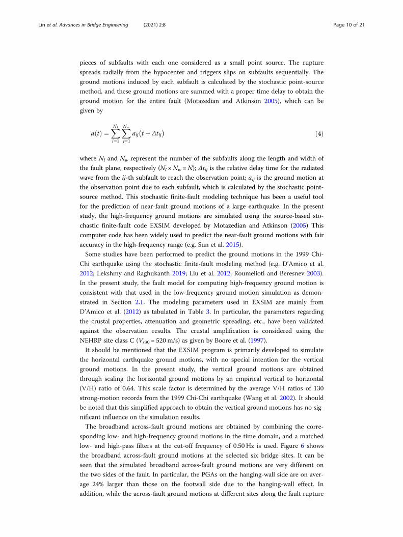
Figure 7 compares the elastic pseudo-acceleration response spectra (5% damping) be-

tween the simulated horizontal across-fault ground motions and the GMPE ASK14. It

can be seen that the mean value of the simulations (blue dashed line) is close to the

Fig. 6 Simulation results of the broadband ground motion time histories at each bridge site: a acceleration;b velocity; c displacement. The number of each subplot indicates the peak value with the unit in cm/s2,cm/s and cm for acceleration, velocity and displacement, respectively. The numbers on the left correspondto the bridges listed in Table 1

Lin et al. Advances in Bridge Engineering (2021) 2:8 Page 12 of 21

ASK14 predicted results (bold red line). The simulation results (12 horizontal ground

motions on the hanging-wall and footwall respectively) are generally within the range

between the predicted value plus or minus one standard deviation. Therefore, it is be-

lieved that the simulation results can give reasonable predictions to the across-fault

ground motions.

It should be mentioned that as can be observed from Fig. 7, some simulation results

exceed the predicted range (i.e. the predicted value plus or minus one standard devi-

ation) in the long period range. This is expected since the simulated across-fault

ground motions are from the observation points located very close to surface rupture,

where large long-period components are prominent due to the fling-step effect. How-

ever, the strong-motion records for the regression of ASK14 distributed over a large

seismic area and can not accurately reflect the local situation very close to the fault.

3 Bridge collapse analyses3.1 Bridge details

In this section, a case study is presented to investigate the collapse failure mechanism

of the fault-crossing bridges in the 1999 Chi-Chi earthquake. As mentioned in Section

2.2, most of the fault-crossing bridges were multi-span simply-supported bridges (see

Table 4 Input parameters for GMPE ASK14

Parameter Value

Moment magnitude 7.6

The closest distance to the ruptured plane, Rrup (km) 0.25/0.5 for hanging-wall/footwall

Joyner-Boore distance, Rjb (km) 0/0.5 for hanging-wall/footwall

Rx (km) 0.5

Ry0 (km) 0

Depth to the top of rupture plane, Ztor (km) 0

Fault dip/rake angle 30°/55°

Down-dip rupture width (km) 44

Region Taiwan

Vs30 (m/s) 520

Fig. 7 Comparison of the elastic pseudo-acceleration response spectra (5% damping) between thesimulated horizontal across-fault ground motions and the GMPE ASK14: a Footwall side; bHanging-wall side

Lin et al. Advances in Bridge Engineering (2021) 2:8 Page 13 of 21

Table 1). Thus, a three-span simply-supported girder bridge with a similar engineering

background is considered herein. Figure 8 shows the geometry of the bridge. In particu-

lar, the superstructure consists of three spans of simply-supported reinforced-concrete

box girders with a length of 30 m for each span (see Fig. 8a and b). The bridge piers are

single-column reinforced concrete bents with a height of 12 m and a rectangular cross-

section of 4.2 × 1.75 m (see Fig. 8d), and they support the bridge girders through two

rows of rubber bearings beneath the girder end of each span. L-type abutments are

placed at the two ends of the entire bridge (see Fig. 8c) to confine the longitudinal

movement of the bridge superstructure. Expansion joints with a gap of 50 mm are in-

troduced between the adjacent girders and abutments where seismic poundings may

occur. With a similar engineering background compared to the fault-crossing bridges

in the Chi-Chi earthquake, it is believed that this bridge model can reflect some essen-

tial characteristics of this type of bridge with respect to structural responses and dam-

age modes under the across-fault ground motions.

3.2 Explicit dynamic FE model

3.2.1 Element and material properties

A detailed 3D explicit dynamic finite element model of the bridge is developed using

ANSYS/LS-DYNA (LSTC 2016). The main structure of the bridge is constructed by

constant stress 8-node solid element, and the reinforcements are modeled by beam

element. The material models MAT_CONCRETE_DAMAGE_REL3 (MAT_072R3) and

MAT_PIECEWISE_LINEAR_PLASTICITY (MAT_024) are adopted to model the con-

crete and reinforcements respectively at the end regions of the bridge girder, as well as

the potential contact sides of the abutments, with a fine mesh size of 60 mm. This

modeling can simulate very detailed damages at the local regions where seismic pound-

ings may occur. The material model MAT_PSEUDO_TENSOR (MAT_016) is used to

model the reinforced concrete of the other parts of the bridge, namely a smeared model

with a coarse mesh is used. The combination of these two modeling techniques for re-

inforced concrete can achieve satisfied simulation results with a relatively low cost of

computational effort, which have been used by many researchers and proven yielding

good results (e.g. Bi and Hao 2013; Lin et al. 2020a; Tang and Hao 2010). The

elastomeric bearing pads supporting each span are modeled by the material model

Fig. 8 Geometry of the bridge: a elevation view; cross-section of b bridge girder, c abutments and dbridge piers (unit: mm)

Lin et al. Advances in Bridge Engineering (2021) 2:8 Page 14 of 21

MAT_VISCOELASTIC (MAT_006). The material properties of the bridge model are

tabulated in Table 5. In addition, MAT_ADD_EROSION is introduced to delete highly

deformed elements when the maximum principal strain reaches 0.15.

The strengths of the structural materials can be enhanced due to the strain rate effect

under dynamic loads. Therefore, the dynamic increase factor (DIF), i.e. a ratio of the

dynamic to static strength against strain rate to account for the material strength en-

hancement with strain rate effect, is utilized to account for the material strength en-

hancement effect for both concrete and reinforcement materials. In the present study,

the bilinear relationship developed by CEB code (Beton CE-Id 1990) and Malvar and

Ross (1998) are applied for the concrete compression and tensile strength enhancement

respectively, and the K&C model (Malvar 1998) is utilized to determine the DIF for the

reinforcement bars.

3.2.2 Boundary conditions and input ground motions

Contacts between the bridge members are considered in the FE model. In particular,

these contacts include the poundings between the adjacent girder segments, the sliding

between girders and bearings, and the frictions between girders and piers. In addition,

the ground surface is modeled with a rigid plane so that the impact between the bridge

girder and the ground surface can be simulated when girder unseating occurs. The con-

tact algorithm CONTACT_AUTOMATIC_SURFACE_TO_SURFACE is employed for

all the potential contact interfaces. By using this contact algorithm, the Coulomb fric-

tion needs to be specified, which is set to be 0.5 in this study (Jankowski 2012).

The bridge model is assumed to cross the surface fault rupture in the normal direc-

tion (see Fig. 9), namely a fault-crossing angle of 90° is considered, and the longitudinal

Table 5 Material properties

Material E (GPa) fc’ (MPa) ft or fy (MPa) ρ (kg/m3)

Concrete – 50 5 2400

Reinforcement 200 – 550 7850

Elastomeric bearing pad 0.182 – – 2300

Fig. 9 Location relationship between the bridge and the fault

Lin et al. Advances in Bridge Engineering (2021) 2:8 Page 15 of 21

and transverse directions of the bridge point to the fault-normal and fault-parallel di-

rections, respectively. The surface fault rupture locates beneath the middle span, and

the left (i.e. Abutment 1 and Pier 1) and right spans (i.e. Abutment 2 and Pier 2) are lo-

cated on Sides 1 and 2, respectively (see Fig. 9). All the bridge supports are fixed on the

ground, namely earthquake excitations are directly applied to all the piers and abut-

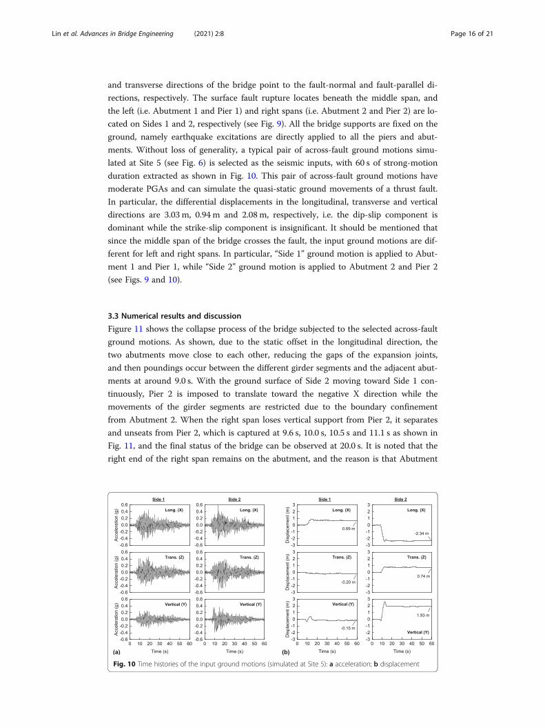
ments. Without loss of generality, a typical pair of across-fault ground motions simu-

lated at Site 5 (see Fig. 6) is selected as the seismic inputs, with 60 s of strong-motion

duration extracted as shown in Fig. 10. This pair of across-fault ground motions have

moderate PGAs and can simulate the quasi-static ground movements of a thrust fault.

In particular, the differential displacements in the longitudinal, transverse and vertical

directions are 3.03 m, 0.94 m and 2.08 m, respectively, i.e. the dip-slip component is

dominant while the strike-slip component is insignificant. It should be mentioned that

since the middle span of the bridge crosses the fault, the input ground motions are dif-

ferent for left and right spans. In particular, “Side 1” ground motion is applied to Abut-

ment 1 and Pier 1, while “Side 2” ground motion is applied to Abutment 2 and Pier 2

(see Figs. 9 and 10).

3.3 Numerical results and discussion

Figure 11 shows the collapse process of the bridge subjected to the selected across-fault

ground motions. As shown, due to the static offset in the longitudinal direction, the

two abutments move close to each other, reducing the gaps of the expansion joints,

and then poundings occur between the different girder segments and the adjacent abut-

ments at around 9.0 s. With the ground surface of Side 2 moving toward Side 1 con-

tinuously, Pier 2 is imposed to translate toward the negative X direction while the

movements of the girder segments are restricted due to the boundary confinement

from Abutment 2. When the right span loses vertical support from Pier 2, it separates

and unseats from Pier 2, which is captured at 9.6 s, 10.0 s, 10.5 s and 11.1 s as shown in

Fig. 11, and the final status of the bridge can be observed at 20.0 s. It is noted that the

right end of the right span remains on the abutment, and the reason is that Abutment

Fig. 10 Time histories of the input ground motions (simulated at Site 5): a acceleration; b displacement

Lin et al. Advances in Bridge Engineering (2021) 2:8 Page 16 of 21

2 provides a sufficient supporting length for the right span when moving toward the

negative X direction.

It also can be noted from Fig. 11 that while unseating does not occur to the other

two spans, certain damages and different final status are however obtained due to the

fault dislocation. In particular, the left and middle spans suffer pounding damages at the girder

ends with the gaps of expansion joints compressed. For the middle span, due to the vertical

static offset of Side 2, its right end is significantly lifted up through Pier 2, higher than the left

end. It should be mentioned that no displacement restriction device exists between the girder

segments and the piers, thus very large relative displacements occur to the elastomeric bearing

pads, which allows the bridge pier to move together with the ground surface with insignificant

damages occurring. Because the longitudinal permanent displacement of Side 2 is much larger

than that of Side 1 as shown in Fig. 10, most of the differential displacement across the fault is

accommodated by the relative displacement between Pier 2 and the middle and right girder

segments (see Fig. 11 when t = 20 s), which therefore resulted in the unseating of the right

span only. It also should be mentioned that in the transverse direction, the response of the

bridge is dominated by the dynamic component, and the reason is that the input ground mo-

tions in the transverse direction have relatively small permanent ground displacements.

As mentioned in Section 2.4, the broadband across-fault ground motions are domi-

nated by the low-frequency components. For comparison, the corresponding low-

Fig. 11 Collapse process of the three-span simply-supported bridge subject to the selected across-faultground motions

Lin et al. Advances in Bridge Engineering (2021) 2:8 Page 17 of 21

frequency across-fault ground motions (see Site 5 in Fig. 5) are also used to excite the

bridge structure, and it is found that the collapse process of the bridge is almost identi-

cal to the results excited by the broadband across-fault ground motions as shown in

Fig. 11. The collapse process is not presented to avoid repetition. Figure 12 compares

the displacement time histories of the right span subjected to the broadband and low-

frequency across-fault ground motions. For a straightforward demonstration, the left

end of the right span is denoted by Point A, and the upper end of the right pier is de-

noted by Point B as shown in Fig. 11. It can be seen from Fig. 12a that the displace-

ment time history of Point A excited by the low-frequency ground motions shows close

peak and residual displacements compared to that excited by the broadband ground

motions. For the relative displacement between Points A and B as shown in Fig. 12b,

very close results are obtained, implying the process of girder unseating due to the

broadband and low-frequency across-fault ground motions are almost the same.

It should be noted that the bridge is assumed to cross the surface fault rupture

in 90°, and the thrust fault generates very large differential displacements in both

longitudinal and vertical directions with most of the static offsets generated on

Side 2 (i.e. the hanging-wall side). This particular boundary condition results in the

above collapse mode of the simply-supported bridge. In fact, similar scenarios were

observed for the fault-crossing bridges in the 1999 Chi-Chi earthquake. For

example, the E-Jian Bridge was a 24-span simply-supported bridge. During the

earthquake, 12 spans in the northern half of the bridge collapsed (see Fig. 13),

while the other 12 spans in the southern half of the bridge remained standing with

minor damages. A field examination indicated that some of the piers in the

northern portion moved towards the center of the river channel as rigid bodies,

Fig. 12 a Longitudinal displacement time histories of Point A; b Longitudinal relative displacement timehistories between Points A and B

Fig. 13 The collapsed spans of the E-Jian Bridge due to surface faulting movement. Images are modifiedfrom Lee and Loh (2000)

Lin et al. Advances in Bridge Engineering (2021) 2:8 Page 18 of 21

while the residual displacements in the southern piers were insignificant (Lee and

Loh 2000). Thus, it is confirmed that the collapse was due to the gross movements

of the northern substructures with relative displacements exceeding the supporting

length of the bridge piers, instead of the excessive structural dynamic vibrations. It

should be mentioned that the elastomeric bearing pads between the superstructure

and the substructure are weak to resist large relative displacements. Thus, displace-

ment restriction devices or isolation bearings may be introduced to reduce the

relative displacements and possibly prevent unseating of the superstructure for

simply-supported bridges crossing fault-rupture zones.

4 ConclusionsIn the present study, the across-fault ground motions at the fault-crossing bridges in

the 1999 Chi-Chi earthquake are simulated using the hybrid deterministic-stochastic

method. A case study is then performed to investigate the seismic collapse mechanism

of a typical simply-supported bridge under the across-fault ground motions. The main

conclusions are summarized as follows:

1. The source-based hybrid deterministic-stochastic method can give reasonable pre-

dictions to the across-fault ground motions, which is useful for the seismic per-

formance analyses of fault-crossing bridges.

2. The case study indicates that under the selected across-fault ground motions, the

simply-supported bridge shows different damage modes on the two sides of the

fault. In particular, unseating occurs to the bridge span on Side 2 (i.e. the hanging-

wall side), while on Side 1 (i.e. the footwall side), pounding damages occur to the

ends of the girder segments.

3. Under the across-fault ground motions with pronounced fling-steps, the structural

responses and collapse mechanism of the simply-supported bridge are dominated

by the low-frequency ground motions. The large differential static offset across the

fault is the main reason for the collapse of the simply-supported bridge.

It should be mentioned that under the across-fault ground motions with pronounced

fling-steps, simply-supported bridges are very vulnerable. Displacement restriction de-

vices and isolation bearings may be applied to mitigate the structural deformations in-

duced by fault dislocation and avoid girder unseating, and this topic deserves further

investigations.

AbbreviationsFE: Finite element; GMPE: Ground motion prediction equation; GPS: Global positioning system; PGA: Peak groundacceleration; PGV: Peak ground velocity; PGD: Peak ground displacement; DIF: Dynamic increase factor

AcknowledgmentsThe fault model from Finite-Source Rupture Model Database is acknowledged.

Authors’ contributionsYuanzheng Lin analyzed the data and was a major contributor in writing the manuscript. Zhouhong Zong providedideas for this manuscript. Jin Lin managed the data analysis. Yale Li graphed the data. Yiyan Chen checked the analysisresults. All authors have read and approved the final manuscript.

FundingThe National Natural Science Foundation of China (51678141).

Lin et al. Advances in Bridge Engineering (2021) 2:8 Page 19 of 21

Availability of data and materialsThe fault model and code for ground motion simulation during the study are available from the corresponding authorby reasonable request. The FE model of the bridge is proprietary and may only be provided with restrictions.

Competing interestsThe authors declare that they have no competing interests.

Author details1Engineering Research Center of Safety and Protection of Explosion & Impact of Ministry of Education (ERCSPEIME),Southeast University, Nanjing 211189, Jiangsu, China. 2School of Civil Engineering, Southeast University, Nanjing211189, Jiangsu, China. 3Department of Building Engineering, Jiangsu Open University, Nanjing 210036, China. 4Schoolof Civil Engineering, Fuzhou University, Fuzhou 350108, China.

Received: 24 October 2020 Accepted: 16 December 2020

ReferencesAbrahamson NA, Silva WJ, Kamai R (2014) Summary of the ASK14 ground motion relation for active crustal regions.

Earthquake Spectra 30(3):1025–1055. https://doi.org/10.1193/070913EQS198MAki K, Richards PG (1980) Quantitative seismology: theory and methods. W. H. Freeman and Company, San FranciscoAnastasopoulos I, Gazetas G, Drosos V, Georgarakos T, Kourkoulis R (2008) Design of bridges against large tectonic

deformation. Earthq Eng Eng Vib 7(4):345–368. https://doi.org/10.1007/s11803-008-1001-xBeton CE-Id (1990) Concrete structures under impact and impulsive loading. CEB Bulletin 187. Federal Institute of

Technology, LausanneBi K, Hao H (2013) Numerical simulation of pounding damage to bridge structures under spatially varying ground motions.

Eng Struct 46:62–76. https://doi.org/10.1016/j.engstruct.2012.07.012Boore DM (1983) Stochastic simulation of high-frequency ground motions based on seismological models of the radiated

spectra. Bull Seismol Soc Am 73(6A):1865–1894Boore DM (2003) Simulation of ground motion using the stochastic method. Pure Appl Geophys 160:635–676Boore DM, Joyner WB, Fumal TE (1997) Equations for estimating horizontal response spectra and peak acceleration from

western north American earthquakes: a summary of recent work. Seismol Res Lett 68(1):128–153. https://doi.org/10.1785/gssrl.68.1.128

Bouchon M (1979) Discrete wave number representation of elastic wave fields in three-space dimensions. J Geophys ResSolid Earth 84(B7):3609–3614

Bouchon M, Aki K (1977) Discrete wave-number representation of seismic-source wave fields. Bull Seismol Soc Am 67(2):259–277

Burridge R, Knopoff L (1964) Body force equivalents for seismic dislocations. Bull Seismol Soc Am 54(6A):1875–1888Chi W-C, Dreger D, Kaverina A (2001) Finite-source modeling of the 1999 Taiwan (Chi-Chi) earthquake derived from a dense

strong-motion network. Bull Seismol Soc Am 91(5):1144–1157. https://doi.org/10.1785/0120000732D’Amico S, Akinci A, Malagnini L (2012) Predictions of high-frequency ground-motion in Taiwan based on weak motion data.

Geophys J Int 189(1):611–628. https://doi.org/10.1111/j.1365-246X.2012.05367.xDing Y, Mavroeidis GP, Theodoulidis NP (2019) Simulation of strong ground motion from the 1995 Mw 6.5 Kozani-Grevena,

Greece, earthquake using a hybrid deterministic-stochastic approach. Soil Dyn Earthq Eng 117:357–373Goel RK, Chopra AK (2009a) Linear analysis of ordinary bridges crossing fault-rupture zones. J Bridg Eng 14(3):203–215.

https://doi.org/10.1061/(ASCE)1084-0702(2009)14:3(203)Goel RK, Chopra AK (2009b) Nonlinear analysis of ordinary bridges crossing fault-rupture zones. J Bridg Eng 14(3):216–224.

https://doi.org/10.1061/(ASCE)1084-0702(2009)14:3(216)Han Q, Du X, Liu J, Li Z, Li L, Zhao J (2009) Seismic damage of highway bridges during the 2008 Wenchuan earthquake.

Earthq Eng Eng Vib 8(2):263–273. https://doi.org/10.1007/s11803-009-8162-0Hui Y (2015) Study on ground motion input and seismic response of bridges crossing active fault. PhD thesis, Southeast

University, NanjingJankowski R (2012) Non-linear FEM analysis of pounding-involved response of buildings under non-uniform earthquake

excitation. Eng Struct 37:99–105. https://doi.org/10.1016/j.engstruct.2011.12.035Ji C, Helmberger DV, Wald DJ, Ma KF (2003) Slip history and dynamic implications of the 1999 Chi-Chi, Taiwan, earthquake. J

Geophys Res Solid Earth 108(B9):2412. https://doi.org/10.1029/2002JB001764Kamae K, Irikura K, Pitarka A (1998) A technique for simulating strong ground motion using hybrid Green's function. Bull

Seismol Soc Am 88(2):357–367Kawashima K, Takahashi Y, Ge H, Wu Z, Zhang J (2009) Reconnaissance report on damage of bridges in 2008 Wenchuan,

China, earthquake. J Earthq Eng 13(7):965–996. https://doi.org/10.1080/13632460902859169Lee GC, Loh C-H (2000) The Chi-Chi, Taiwan earthquake of September 21, 1999: reconnaissance report. The Multidisciplinary

Center for Earthquake Engineering Research, State University of New York at Buffalo, BuffaloLekshmy P, Raghukanth S (2019) Stochastic earthquake source model for ground motion simulation. Earthq Eng Eng Vib

18(1):1–34Lin Y, Chen Y, Zong Z, Lin J, Tang G, He X (2021) A new hybrid input strategy to reproduce across-fault ground motions on

multi-shaking tables. J Test Eval 49(2):20190797. https://doi.org/10.1520/JTE20190797Lin Y, Zong Z, Bi K, Hao H, Lin J, Chen Y (2020a) Experimental and numerical studies of the seismic behavior of a steel-

concrete composite rigid-frame bridge subjected to the surface rupture at a thrust fault. Eng Struct 205:110105. https://doi.org/10.1016/j.engstruct.2019.110105

Lin Y, Zong Z, Bi K, Hao H, Lin J, Chen Y (2020b) Numerical study of the seismic performance and damage mitigation ofsteel–concrete composite rigid-frame bridge subjected to across-fault ground motions. Bull Earthq Eng 18(15):6687–6714.https://doi.org/10.1007/s10518-020-00958-1

Lin et al. Advances in Bridge Engineering (2021) 2:8 Page 20 of 21

Lin Y, Zong Z, Tian S, Lin J (2018) A new baseline correction method for near-fault strong-motion records based on thetarget final displacement. Soil Dyn Earthq Eng 114:27–37. https://doi.org/10.1016/j.soildyn.2018.06.036

Liu T, Atkinson GM, Hong H, Assatourians K (2012) Intraevent spatial correlation characteristics of stochastic finite-faultsimulations. Bull Seismol Soc Am 102(4):1740–1747

LSTC (2016) LS-DYNA keyword user’s manual R9.0. Livermore Software Technology Corporation, LivermoreMa K-F, Mori J, Lee S-J, Yu S (2001) Spatial and temporal distribution of slip for the 1999 Chi-Chi, Taiwan, earthquake. Bull

Seismol Soc Am 91(5):1069–1087. https://doi.org/10.1785/0120000728Mai PM. Finite-Source Rupture Model Database (SRCMOD). 2015. http://equake-rc.info/SRCMOD/Malvar LJ (1998) Review of static and dynamic properties of steel reinforcing bars. ACI Mater J 95(5):609–616Malvar LJ, Ross CA (1998) Review of strain rate effects for concrete in tension. ACI Mater J 95(6):735–739Motazedian D, Atkinson GM (2005) Stochastic finite-fault modeling based on a dynamic corner frequency. Bull Seismol Soc

Am 95(3):995–1010NCREE (2002) 921 Chi-Chi earthquake on-line museum. National Center for Research on Earthquake Engineering http://www.

ncree.org/921_bridge_project/Olson AH, Orcutt JA, Frazier GA (1984) The discrete wavenumber/finite element method for synthetic seismograms. Geophys

J Int 77(2):421–460. https://doi.org/10.1111/j.1365-246X.1984.tb01942.xPamuk A, Kalkan E, Ling H (2005) Structural and geotechnical impacts of surface rupture on highway structures during recent

earthquakes in Turkey. Soil Dyn Earthq Eng 25(7–10):581–589. https://doi.org/10.1016/j.soildyn.2004.11.011Papageorgiou AS (2003) The barrier model and strong ground motion. Pure Appl Geophys 160(3–4):603–634Park S, Ghasemi H, Shen J, Somerville P, Yen W, Yashinsky M (2004) Simulation of the seismic performance of the Bolu

Viaduct subjected to near-fault ground motions. Earthq Eng Struct Dyn 33(13):1249–1270. https://doi.org/10.1002/eqe.395Roumelioti Z, Beresnev IA (2003) Stochastic finite-fault modeling of ground motions from the 1999 Chi-Chi, Taiwan,

earthquake: application to rock and soil sites with implications for nonlinear site response. Bull Seismol Soc Am 93(4):1691–1702. https://doi.org/10.1785/0120020218

Roussis PC, Constantinou MC, Erdik M, Durukal E, Dicleli M (2003) Assessment of performance of seismic isolation system ofBolu Viaduct. J Bridg Eng 8(4):182–190. https://doi.org/10.1061/(ASCE)1084-0702(2003)8:4(182)

Saiidi MS, Vosooghi A, Choi H, Somerville P (2013) Shake table studies and analysis of a two-span RC bridge model subjectedto a fault rupture. J Bridg Eng 19(8):A4014003. https://doi.org/10.1061/(ASCE)BE.1943-5592.0000478

Shin T-C, Teng T-l (2001) An overview of the 1999 Chi-Chi, Taiwan, earthquake. Bull Seismol Soc Am 91(5):895–913.https://doi.org/10.1785/0120000738

Somerville PG (2002) Characterizing near fault ground motion for the design and evaluation of bridges. In: 3rd nationalseismic conference and workshop on bridges and highways, Portland, Oregon

Spudich P, Archuleta RJ (1987) Techniques for earthquake ground-motion calculation with applications to sourceparameterization of finite faults. In: Bolt BA (ed) Seismic strong motion synthetics. Academic, Orlando, pp 205–265

Sun X, Hartzell S, Rezaeian S (2015) Ground-motion simulation for the 23 August 2011, Mineral, Virginia, earthquake usingphysics-based and stochastic broadband methods. Bull Seismol Soc Am 105(5):2641–2661

Tang EK, Hao H (2010) Numerical simulation of a cable-stayed bridge response to blast loads, part I: model development andresponse calculations. Eng Struct 32(10):3180–3192. https://doi.org/10.1016/j.engstruct.2010.06.007

Ucak A, Mavroeidis GP, Tsopelas P (2014) Behavior of a seismically isolated bridge crossing a fault rupture zone. Soil DynEarthq Eng 57:164–178. https://doi.org/10.1016/j.soildyn.2013.10.012

Wang G-Q, Zhou X-Y, Zhang P-Z, Igel H (2002) Characteristics of amplitude and duration for near fault strong ground motionfrom the 1999 Chi-Chi, Taiwan earthquake. Soil Dyn Earthq Eng 22(1):73–96. https://doi.org/10.1016/S0267-7261(01)00047-1

Wu C, Takeo M, Ide S (2001) Source process of the Chi-Chi earthquake: a joint inversion of strong motion data and globalpositioning system data with a multifault model. Bull Seismol Soc Am 91(5):1128–1143. https://doi.org/10.1785/0120000713

Yang S, Mavroeidis GP (2018) Bridges crossing fault rupture zones: a review. Soil Dyn Earthq Eng 113:545–571.https://doi.org/10.1016/j.soildyn.2018.03.027

Yang S, Mavroeidis GP, Ucak A (2020) Analysis of bridge structures crossing strike-slip fault rupture zones: a simplemethod for generating across-fault seismic ground motions. Earthq Eng Struct Dyn 49(13):1281–1307.https://doi.org/10.1002/eqe.3290

Zhang F, Li S, Wang J, Zhang J (2020) Effects of fault rupture on seismic responses of fault-crossing simply-supportedhighway bridges. Eng Struct 206:110104. https://doi.org/10.1016/j.engstruct.2019.110104

Publisher’s NoteSpringer Nature remains neutral with regard to jurisdictional claims in published maps and institutional affiliations.

Lin et al. Advances in Bridge Engineering (2021) 2:8 Page 21 of 21