Embed Size (px)
Citation preview
Lab Manual – Advanced Communication Systems
Vishwakarma Institute of Information Technology, Pune 1
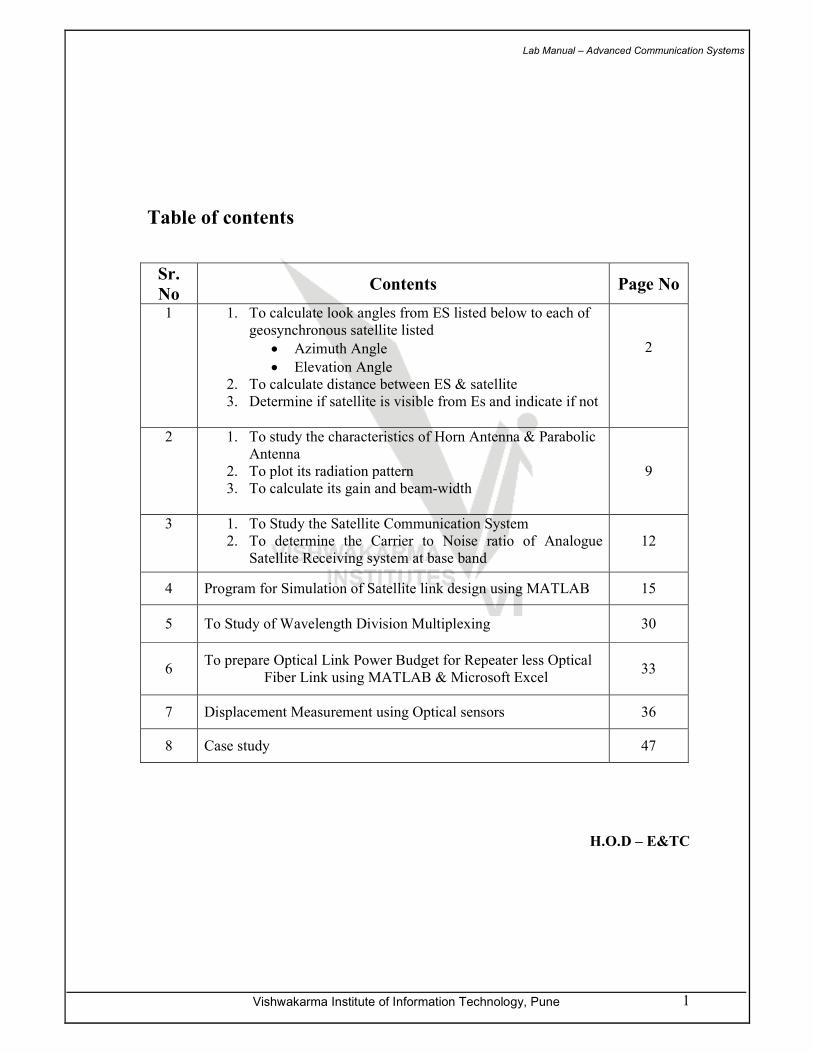
Table of contents
Sr.
No Contents Page No
1 1. To calculate look angles from ES listed below to each of
geosynchronous satellite listed
• Azimuth Angle
• Elevation Angle
2. To calculate distance between ES & satellite
3. Determine if satellite is visible from Es and indicate if not
2
2 1. To study the characteristics of Horn Antenna & Parabolic
Antenna
2. To plot its radiation pattern
3. To calculate its gain and beam-width
9
3 1. To Study the Satellite Communication System
2. To determine the Carrier to Noise ratio of Analogue
Satellite Receiving system at base band
12
4 Program for Simulation of Satellite link design using MATLAB 15
5 To Study of Wavelength Division Multiplexing 30
6 To prepare Optical Link Power Budget for Repeater less Optical
Fiber Link using MATLAB & Microsoft Excel 33
7 Displacement Measurement using Optical sensors 36
8 Case study 47
H.O.D – E&TC

Lab Manual – Advanced Communication Systems
Vishwakarma Institute of Information Technology, Pune 2
EXPERIMENT NO: 01
TITLE OF EXPERIMENT :
4. To calculate look angles from ES listed below to each of
geosynchronous satellite listed
• Azimuth Angle
• Elevation Angle
5. To calculate distance between ES & satellite
6. Determine if satellite is visible from Es and indicate if not
Lab Manual – Advanced Communication Systems
Vishwakarma Institute of Information Technology, Pune 3
1.1 Aim: 7. To calculate look angles from ES listed below to each of geosynchronous satellite
listed
• Azimuth Angle
• Elevation Angle
8. To calculate distance between ES & satellite
9. Determine if satellite is visible from Es and indicate if not
Earth Station
1. 44° 48' 59'' N
70° 42' 52'' W
2. 24° 52' 13'' S
113° 42' 13'' E
Satellites
1. 87° W
2. 127.5° W
3. 110° E
1.2 Theory: 1. Elevation Angle: It is the angle measured upward from the local horizontal plane
at ES to the Satellite path
Cos (EL) = __________Sin (r)_________
[1 + (re/rs) ² – 2(re/rs) Cos(r)] ½
Cos (r) = Cos (le) Cos (ls-le)
…… for geosynchronous
2. Azimuth Angle: It is the angle measured eastward(clockwise) from geographic
north to the projection of satellite path on a locally horizontal plane at ES
S = _a + c+ r_ a = ls-le
2 c = Le
Tan² (α / 2) = _Sin(s-r) Sin (s-c)_
Sin(s-a) Sin (s)
Case 1:-
• Satellite to SE of ES :- Az = 180 – α
• Satellite to SW of ES :- Az = 180 + α
Case 2:-
• Satellite to NE of ES :- Az = α
• Satellite to NW of ES :- Az = 360° - α
3. Distance between ES and satellite is given by-
d = [rs² + re² -2 (re)Cos(r)] ½
4. For a satellite to be visible from ES, its EI must be above some min value, which
is at least 0°. A positive or zero EI requires that-
rs ≥ __re__
Cos(r)
1.3 Result: Comparison of Matlab and Theoretical output
Lab Manual – Advanced Communication Systems
Vishwakarma Institute of Information Technology, Pune 4
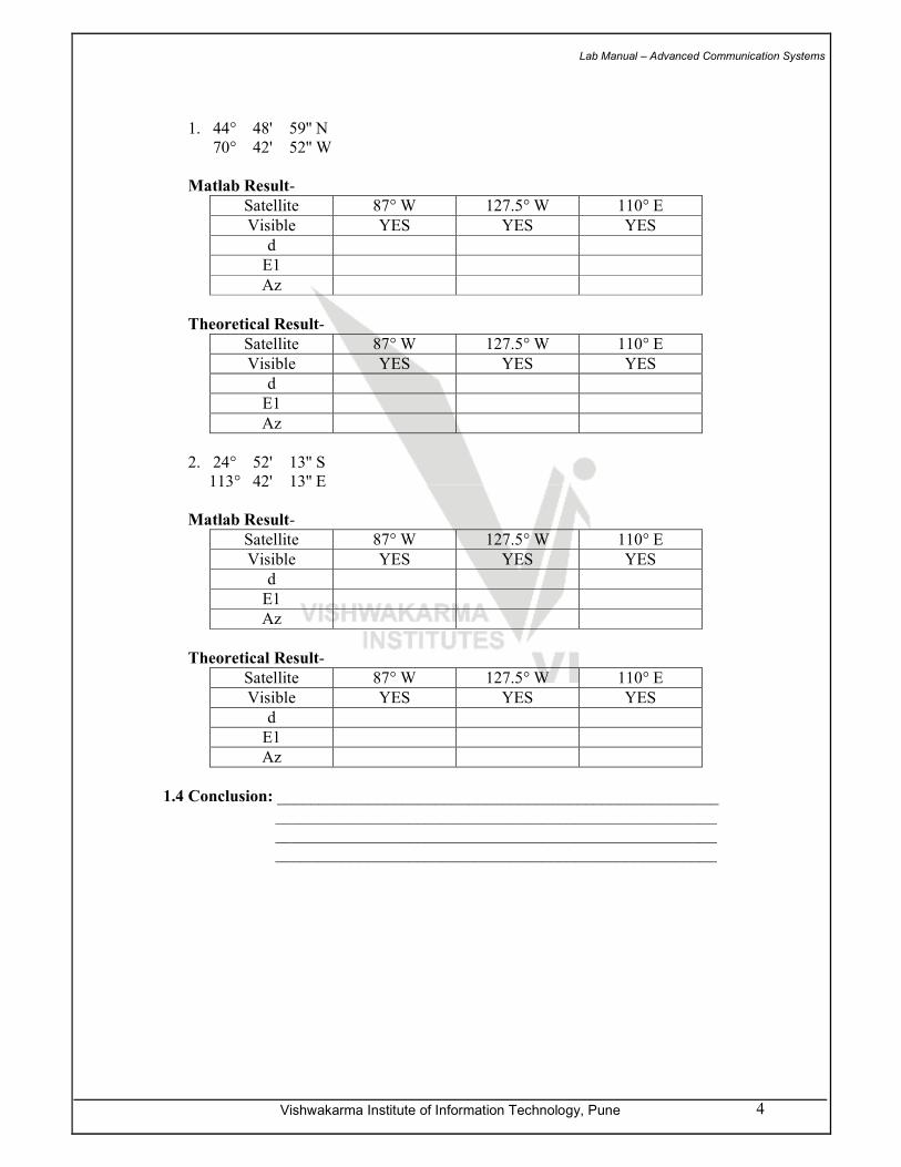
1. 44° 48' 59'' N
70° 42' 52'' W
Matlab Result-
Satellite 87° W 127.5° W 110° E
Visible YES YES YES
d
E1
Az
Theoretical Result-
Satellite 87° W 127.5° W 110° E
Visible YES YES YES
d
E1
Az
2. 24° 52' 13'' S
113° 42' 13'' E
Matlab Result-
Satellite 87° W 127.5° W 110° E
Visible YES YES YES
d
E1
Az
Theoretical Result-
Satellite 87° W 127.5° W 110° E
Visible YES YES YES
d
E1
Az
1.4 Conclusion: _____________________________________________________
_____________________________________________________
_____________________________________________________
_____________________________________________________
Lab Manual – Advanced Communication Systems
Vishwakarma Institute of Information Technology, Pune 5
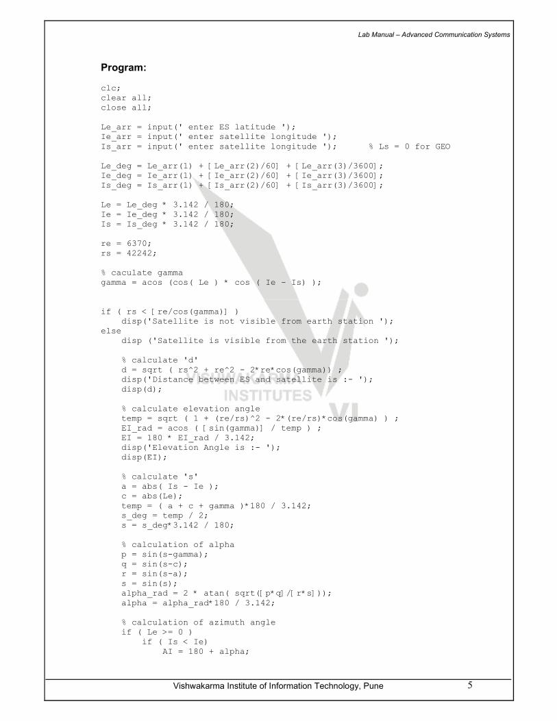
Program: clc; clear all; close all; Le_arr = input(' enter ES latitude '); Ie_arr = input(' enter satellite longitude '); Is_arr = input(' enter satellite longitude '); % Ls = 0 for GEO Le_deg = Le_arr(1) + [Le_arr(2)/60] + [Le_arr(3)/3600]; Ie_deg = Ie_arr(1) + [Ie_arr(2)/60] + [Ie_arr(3)/3600]; Is_deg = Is_arr(1) + [Is_arr(2)/60] + [Is_arr(3)/3600]; Le = Le_deg * 3.142 / 180; Ie = Ie_deg * 3.142 / 180; Is = Is_deg * 3.142 / 180; re = 6370; rs = 42242; % caculate gamma gamma = acos (cos( Le ) * cos ( Ie - Is) ); if ( rs < [re/cos(gamma)] ) disp('Satellite is not visible from earth station '); else disp ('Satellite is visible from the earth station '); % calculate 'd' d = sqrt ( rs^2 + re^2 - 2*re*cos(gamma)) ; disp('Distance between ES and satellite is :- '); disp(d); % calculate elevation angle temp = sqrt ( 1 + (re/rs)^2 - 2*(re/rs)*cos(gamma) ) ; EI_rad = acos ( [sin(gamma)] / temp ) ; EI = 180 * EI_rad / 3.142; disp('Elevation Angle is :- '); disp(EI); % calculate 's' a = abs( Is - Ie ); c = abs(Le); temp = ( a + c + gamma )*180 / 3.142; s_deg = temp / 2; s = s_deg*3.142 / 180; % calculation of alpha p = sin(s-gamma); q = sin(s-c); r = sin(s-a); s = sin(s); alpha_rad = 2 * atan( sqrt([p*q]/[r*s])); alpha = alpha_rad*180 / 3.142; % calculation of azimuth angle if ( Le >= 0 ) if ( Is < Ie) AI = 180 + alpha;
Lab Manual – Advanced Communication Systems
Vishwakarma Institute of Information Technology, Pune 6
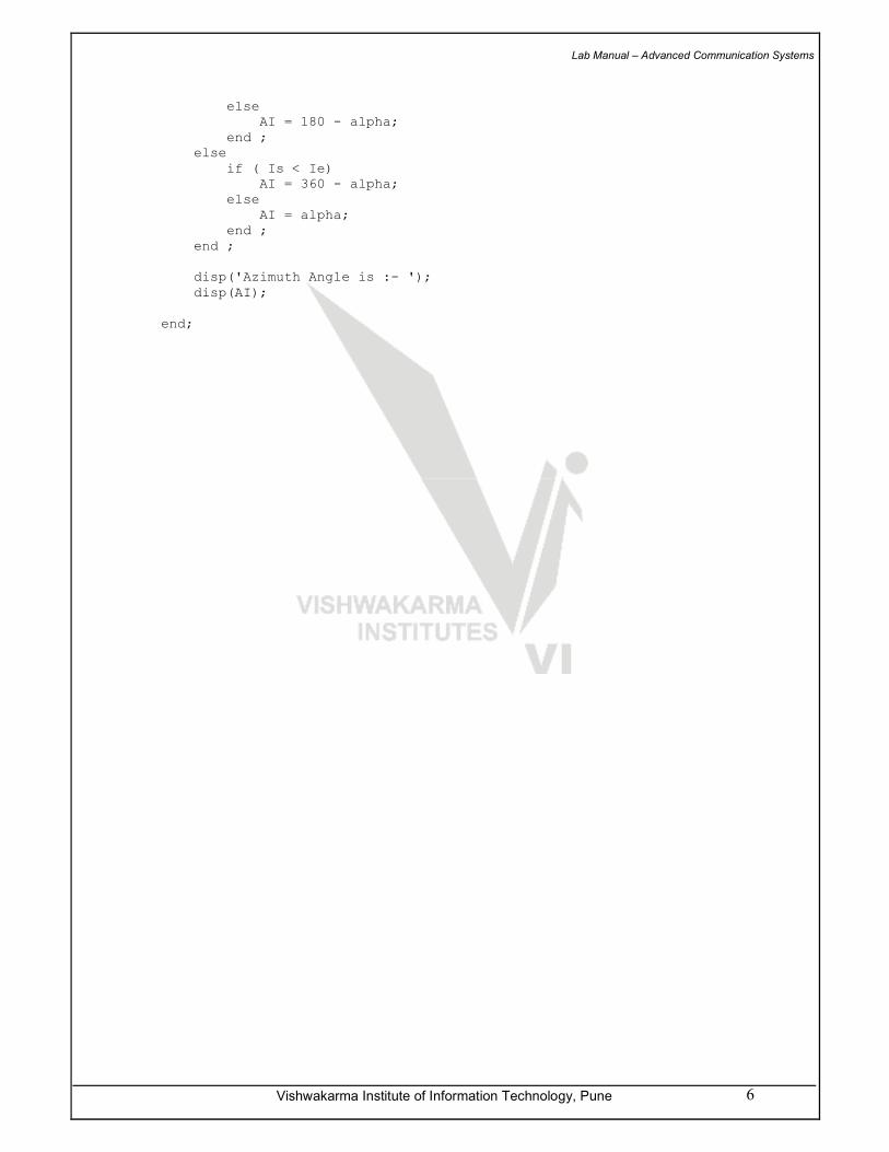
else AI = 180 - alpha; end ; else if ( Is < Ie) AI = 360 - alpha; else AI = alpha; end ; end ; disp('Azimuth Angle is :- '); disp(AI); end;
Lab Manual – Advanced Communication Systems
Vishwakarma Institute of Information Technology, Pune 7
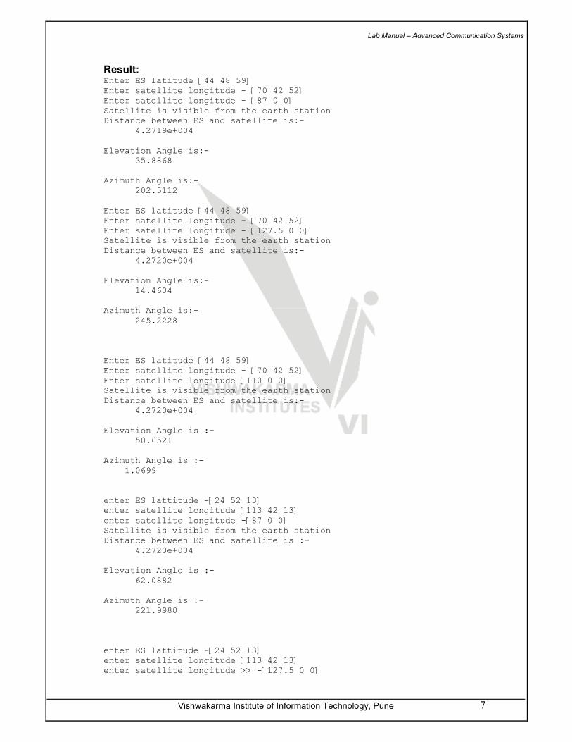
Result: Enter ES latitude [44 48 59] Enter satellite longitude - [70 42 52] Enter satellite longitude - [87 0 0] Satellite is visible from the earth station Distance between ES and satellite is:-
4.2719e+004 Elevation Angle is:-
35.8868 Azimuth Angle is:-
202.5112 Enter ES latitude [44 48 59] Enter satellite longitude - [70 42 52] Enter satellite longitude - [127.5 0 0] Satellite is visible from the earth station Distance between ES and satellite is:-
4.2720e+004 Elevation Angle is:-
14.4604 Azimuth Angle is:-
245.2228 Enter ES latitude [44 48 59] Enter satellite longitude - [70 42 52] Enter satellite longitude [110 0 0] Satellite is visible from the earth station Distance between ES and satellite is:-
4.2720e+004 Elevation Angle is :-
50.6521 Azimuth Angle is :- 1.0699 enter ES lattitude -[24 52 13] enter satellite longitude [113 42 13] enter satellite longitude -[87 0 0] Satellite is visible from the earth station Distance between ES and satellite is :-
4.2720e+004 Elevation Angle is :-
62.0882 Azimuth Angle is :-
221.9980 enter ES lattitude -[24 52 13] enter satellite longitude [113 42 13] enter satellite longitude >> -[127.5 0 0]
Lab Manual – Advanced Communication Systems
Vishwakarma Institute of Information Technology, Pune 8
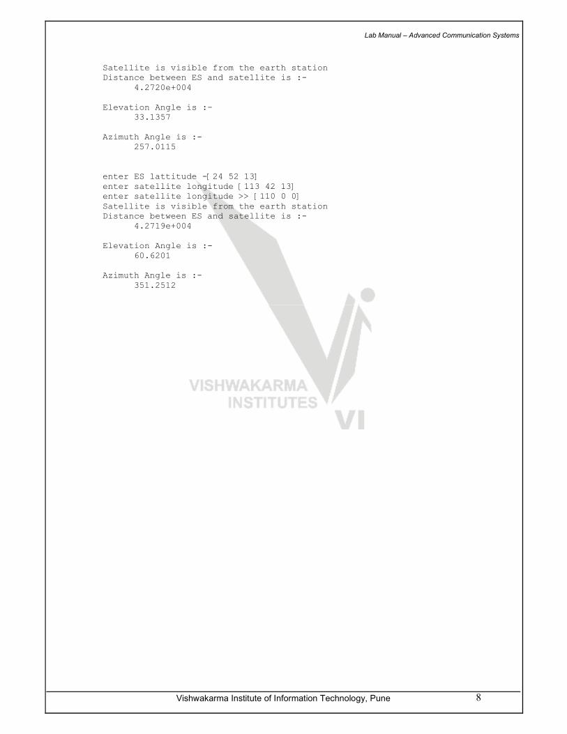
Satellite is visible from the earth station Distance between ES and satellite is :-
4.2720e+004 Elevation Angle is :-
33.1357 Azimuth Angle is :-
257.0115 enter ES lattitude -[24 52 13] enter satellite longitude [113 42 13] enter satellite longitude >> [110 0 0] Satellite is visible from the earth station Distance between ES and satellite is :-
4.2719e+004 Elevation Angle is :-
60.6201 Azimuth Angle is :-
351.2512
Lab Manual – Advanced Communication Systems
Vishwakarma Institute of Information Technology, Pune 9
EXPERIMENT NO: 02
TITLE OF EXPERIMENT : 4. To study the characteristics of Horn Antenna & Parabolic Antenna
5. To plot its radiation pattern 6. To calculate its gain and beam-width
Lab Manual – Advanced Communication Systems
Vishwakarma Institute of Information Technology, Pune 10
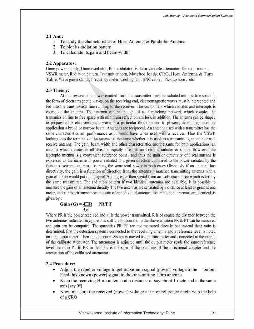
2.1 Aim:
1. To study the characteristics of Horn Antenna & Parabolic Antenna
2. To plot its radiation pattern
3. To calculate its gain and beam-width
2.2 Apparatus:
Gunn power supply, Gunn oscillator, Pin modulator, isolator variable attenuator, Detector mount,
VSWR meter, Radiation pattern, Transmitter horn, Matched loads, CRO, Horn Antenna & Turn
Table, Wave guide stands, Frequency meter, Cooling fan , BNC cable , Pick up horn , etc
2.3 Theory:
At microwaves, the power emitted from the transmitter must be radiated into the free space in
the form of electromagnetic waves, on the receiving end, electromagnetic waves must b intercepted and
fed into the transmission line running to the receiver. The component which radiates and intercepts is
course of the antenna. The antenna can be thought of as a matching network which couples the
transmission line to free space with minimum reflection am loss, in addition. The antenna can be shaped
to propagate the electromagnetic wave in a particular direction and to present, depending upon the
application a broad or narrow beam. Antennas are reciprocal. An antenna used with a transmitter has the
same characteristics am performance as it would have when used with a receiver. Thus the VSWR
looking into the terminals of an antenna is the same whether it is used as a transmitting antenna or as a
receive antenna. The gain, beam width and other characteristics are the same for both applications, an
antenna which radiates in all direction equally is called an isotropic radiator or source. HOW ever the
isotropic antenna is a convenient reference point , and thus the gain or directivity of ; real antenna is
expressed as the increase in power radiated in a given direction compared to the power radiated by the
fictitious isotropic antenna, assuming the same total power in both cases Obviously if an antenna has
directivity, the gain is a function of direction from the antenna .; matched transmitting antenna with a
gain of 20 db would put out a signal 20 db greater then signal from an isotropic source which is fed by
the same transmitter. The radiation pattern if two identical antennas are available, It is possible to
measure the gain of an antenna directly The two antennas are separated by a distance at least as great as one
meter, under these circumstances the gain of an individual antenna .assuming both antennas are identical, is
given by :
Gain (G) = 4ΠΠΠΠR PR/PT
λλλλo Where PR is the power received and PT is the power transmitted. R is of course the distance between the
two antennas indicated in figure 7 is sufficient accurate. In the above equation PR & PT can be measured
and gain can be computed. The quantities PR PT are not measured directly but instead their ratio is
determined, first the detection system i connected to the receiving antenna and a reference level is noted
on the output meter. Then the detection system is moved to the transmitter and connected at the output
of the calibrate attenuator. The attenuator is adjusted until the output meter reads the same reference
level the ratio PT to PR in decibels is the sum of the coupling of the directional coupler and the
attenuation of the calibrated attenuator.
2.4 Procedure:
• Adjust the repeller voltage to get maximum signal (power) voltage a the output
Feed this known (power) signal to the transmitting Horn antenna
• Keep the receiving Horn antenna at a distance of say about 1 mete and in the same
axis [say 0°]
• Now, measure the received (power) voltage at 0° or reference angle with the help
of a CRO

Lab Manual – Advanced Communication Systems
Vishwakarma Institute of Information Technology, Pune 11
• Then, rotate the Horn antenna at 10°, 20°, ....... 90° in left and right hand side and
tabulate the reading from CRO
• Plot the graph on a polar sheet & find its beam-width
2.5 Observation table:
Signal Level (v)
Angle (°)
Left
Right
0
10
20
30
40
50
60
70
80
90
2.6 Calculation of Gain:
Gain (Theoretical) = 4ππππA/ππππλλλλo² Where,
A = a.b/2
a = width of horn
b = height of horn
λλλλo = free space wave length
Gain (Practical) = 4ππππR/λλλλo ⋅⋅⋅⋅ √√√√ Pr/ Pt Where,
R = distance between Transmitter & Receiver
Pt= Transmitted power
Pr= Received Power
2.7 Result:
• The characteristics of given Horn Antenna [E-H plane] is studied
• The radiation pattern is plotted
• The calculated beam-width= ______°
• The gain of Horn Antenna = ______ dB
2.8 Conclusion: _____________________________________________________
_____________________________________________________
_____________________________________________________
_____________________________________________________
Lab Manual – Advanced Communication Systems
Vishwakarma Institute of Information Technology, Pune 12
EXPERIMENT NO: 03
TITLE OF EXPERIMENT : 3. To Study the Satellite Communication System
4. To determine the Carrier to Noise ratio of Analogue Satellite Receiving
system at base band
Lab Manual – Advanced Communication Systems
Vishwakarma Institute of Information Technology, Pune 13
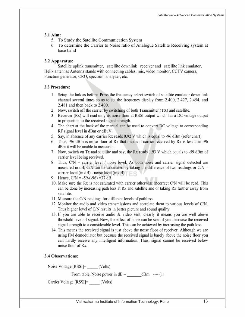
3.1 Aim:
5. To Study the Satellite Communication System
6. To determine the Carrier to Noise ratio of Analogue Satellite Receiving system at
base band
3.2 Apparatus:
Satellite uplink transmitter, satellite downlink receiver and satellite link emulator,
Helix antennas Antenna stands with connecting cables, mic, video monitor, CCTV camera,
Function generator, CRO, spectrum analyzer, etc.
3.3 Procedure:
1. Setup the link as before. Press the frequency select switch of satellite emulator down link
channel several times so as to set the frequency display from 2.400, 2.427, 2.454, and
2.481 and then back to 2.400.
2. Now, switch off the carrier by switching of both Transmitter (TX) and satellite.
3. Receiver (Rx) will read only its noise floor at RSSI output which has a DC voltage output
in proportion to the received signal strength.
4. The chart at the back of the manual can be used to convert DC voltage to corresponding
RF signal level in dBm or dBuV.
5. Say, in absence of any carrier Rx reads 0.92 V which is equal to -96 dBm (refer chart).
6. Thus, -96 dBm is noise floor of Rx that means if carrier received by Rx is less than -96
dBm it will be unable to measure it.
7. Now, switch on Tx and satellite and say, the Rx reads 1.93 V which equals to -59 dBm of
carrier level being received.
8. Thus, C/N = carrier level / noise level. As both noise and carrier signal detected are
measured in dB, C/N can be calculated by taking the difference of two readings or C/N =
carrier level (in dB) - noise level (in dB).
9. Hence, C/N = -59-(-96) =37 dB.
10. Make sure the Rx is not saturated with carrier otherwise incorrect C/N will be read. This
can be done by increasing path loss at Rx and satellite and or taking Rx farther away from
satellite.
11. Measure the C/N readings for different levels of pathless.
12. Monitor the audio and video transmissions and correlate them to various levels of C/N.
Thus higher level of C/N results in better picture and sound quality.
13. If you are able to receive audio & video sent, clearly it means you are well above
threshold level of signal. Now, the effect of noise can be seen if you decrease the received
signal strength to a considerable level. This can be achieved by increasing the path loss.
14. This means the received signal is just above the noise floor of receiver. Although we are
using FM demodulator but because the received signal is barely above the noise floor you
can hardly receive any intelligent information. Thus, signal cannot be received below
noise floor of Rx.
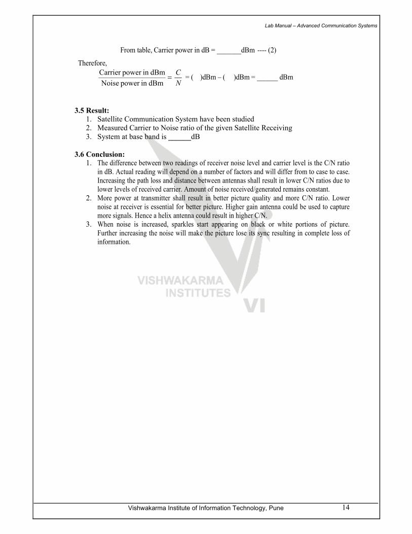
3.4 Observations:
Noise Voltage [RSSI]= _____ (Volts)
From table, Noise power in dB = _______dBm ---- (1)
Carrier Voltage [RSSI]= _____ (Volts)
Lab Manual – Advanced Communication Systems
Vishwakarma Institute of Information Technology, Pune 14
From table, Carrier power in dB = _______dBm ---- (2)
Therefore,
=dBmin power Noise
dBmin power Carrier
N
C = ( )dBm – ( )dBm = ______ dBm
3.5 Result: 1. Satellite Communication System have been studied
2. Measured Carrier to Noise ratio of the given Satellite Receiving
3. System at base band is ______dB
3.6 Conclusion:
1. The difference between two readings of receiver noise level and carrier level is the C/N ratio
in dB. Actual reading will depend on a number of factors and will differ from to case to case.
Increasing the path loss and distance between antennas shall result in lower C/N ratios due to
lower levels of received carrier. Amount of noise received/generated remains constant.
2. More power at transmitter shall result in better picture quality and more C/N ratio. Lower
noise at receiver is essential for better picture. Higher gain antenna could be used to capture
more signals. Hence a helix antenna could result in higher C/N.
3. When noise is increased, sparkles start appearing on black or white portions of picture.
Further increasing the noise will make the picture lose its sync resulting in complete loss of
information.
Lab Manual – Advanced Communication Systems
Vishwakarma Institute of Information Technology, Pune 15
EXPERIMENT NO: 04
TITLE OF EXPERIMENT : Program for Simulation of Satellite link
design using MATLAB
Lab Manual – Advanced Communication Systems
Vishwakarma Institute of Information Technology, Pune 16
Program No. 1
A regional Satellite Communication System using 4/6 GHz band has following
parameters.
Satellite
1. Transponder Gain variable between 85 to 100 dB
2. Transponder Bandwidth 36 MHz
3. Transponder peak output power 6.3 watt
4. Antenna Gain (Transmit) 20 dB
5. Antenna Gain (Receiver) 22 dB
6. Satellite Receiver noise temperature 100° K
Earth Station
1. Antenna Gain (Transmit) 61.3 dB
2. Antenna Gain (Receiver) 60.0 dB
3. Receiver Noise Temp 100° K
Four Identical earth stations share one transponder in an FDMA mode. The
allocated channel capacities and B.W are:
Station 1 and Station 2, 132 channels/ 10 MHz BW
Station 3 and station 4, 24 channels/ 5 MHz BW
Assume, in FDMA mode. Transponder is operated at 5 dB output back off to minimize
the IM noise.
Slant distance is such that
FSL Uplink 200 dB
FSL Downlink 196 dB
Determine the following:
• Assuming Earth Station to be located at center of beam coverage, determine the transmitter power required for E.S, if transponder gain setting is at 90dB.
• Determine C/N at receiving E.S. for station 1 and station 3, assuming that these station are located at 3 dB contour of satellite foot print.
• Assuming station 1 and station 3 at 3 dB contour and station 2 and station 4 of beam centre, determine transmitter power levels for E.S.1 and E.S. 4 , if we have
to get minimum weighted signal to noise ratio 47 dB in any worst channel for
station 1 to station 2 and station 4 and station 3
Assume - a) Standard pre-emphasis filters are used.
b) I.M. Noise to be negligible
c) Terrestrial interference noise 1000 pwpo
d) Satellite interference 2000 pwpo

Lab Manual – Advanced Communication Systems
Vishwakarma Institute of Information Technology, Pune 17
Program No. 2
A Satellite provides direct television broadcast service in USA with beam width
1° wide at 3 dB points. The uplink frequency is 30 GHz and down rank frequency is 42
GHz. The Satellite supports two transponders, with each capable of relay one television
channel.
Receiving station uses antenna of 0.8 meter diameter (Assume η= 0.60), an
antenna random (to prevent build up of snow) with loss of 1 dB when the surface is wet.
A LNA is directly mounted on antenna feed with noise figure of 7.0 dB at ambient
temperature of 17° C
The TV signal with video BW of 4.2 MHz is frequency modulated on uplink freq
and occupies the R.F. Bandwidth of 30 MHz
Determine the following:
1. G/T ratio of Receiving Station.
2. C/N for I.F. bandwidth of 30 MHz for receiver, if satellite transmitter has power
output of 1 watt (Assume No losses in Atmosphere, coupling etc.)
3. C/N for receiver located at the edge of the coverage zone(i.e.3 dB contour point),
Assuming (a) 1 dB clear air atmospheric loss, ( b) Attenuation due to Rain is 10
dB, (c) pointing error of 0.33° in receiving antenna.
4. Assuming FM threshold for domestic receivers is 13 dB; determine minimum
power output of transponder to provide satisfactory service of receivers located at
‘C’ above.
Lab Manual – Advanced Communication Systems
Vishwakarma Institute of Information Technology, Pune 18
Program No. 3
A Ku - band Satellite carries a number of narrow bandwidth transponders to
permit communications between small earth stations. The major parameters of satellite
are given below.
Parameter Uplink Downlink
Frequency 14.9 GHz 11.30 GHz
3 dB contour zone of antenna 3.6° x 2.4° 3.6° x 2.4°
Antenna efficiency 65% 65%
Transponder output power (saturated) ----- 20 watt
Transponder I/P noise Temp 520° K -----
Transponder gain, B.W 125dB, 5MHz -----
Pointing Accuracy +1°
Assume the slant distance between E.S. and Satellite - 39000 Km
Determine following:
1. Assuming Satellite Antennas to be having rectangular shape, dimension of
transmitting and receiving antennas in meters and gains of antennas in dB.
2. Determine the power flux density at the center of the coverage area, when
transponders are fully saturated. What is the flux density at the edge of the
coverage zone?
3. Determine the G/T of E.S. located at the edge of the coverage zone to achieve C/N
of 22 dB in 5 MHz bandwidth when transponder in fully saturated by single
carrier.
4. Determine the G/T of E.S. located at edge of the coverage zone to achieve C/N of
10 dB in the bandwidth of 50 kHz, when 20 carriers access the transponders with
equal power, simultaneously and transponder is used at 5.0 dB back- off at the
output.
5. Determine E.S. ‘EIRP’ to fully load the transponder up to saturation with single
carrier.
Lab Manual – Advanced Communication Systems
Vishwakarma Institute of Information Technology, Pune 19
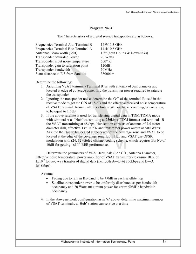
Program No. 4
The Characteristics of a digital service transponder are as follows.
Frequencies Terminal A to Terminal B 14.9/11.3 GHz
Frequencies Terminal B to Terminal A 14.4/10.8 GHz
Antennae Beam width (3dB) 1.5° (both Uplink & Downlinks)
Transponder Saturated Power 20 Watts
Transponder input noise temperature 500° K
Transponder gain to saturation point 120dB
Transponder bandwidth 50MHz
Slant distance to E.S from Satellite 38000km
Determine the following:
1. Assuming VSAT terminal (Terminal B) is with antenna of 3mt diameter and
located at edge of coverage zone, find the transmitter power required to saturate
the transponder
2. Ignoring the transponder noise, determine the G/T of the terminal B used in the
receive mode to get the C/N of 18 dB and the effective received noise temperature
of VSAT terminal. Assume all other losses (Atmospheric, coupling, polarization)
to be equal to 1.5dB
3. If the above satellite is used for transferring digital data in TDM/TDMA mode
with terminal A as ‘Hub’ transmitting at 256kbps (TDM format) and terminal –B
the VSAT transmitting at 48kbps. Hub station consists of antenna of 7.5 meter
diameter dish, effective Ts=100° K and transmitter power output as 500 Watts.
Assume the Hub to be located at the center of the coverage zone and VSAT to be
located at the edge of the coverage zone. Both Hub and VSAT use QPSK
modulation with (24, 12) Goley channel coding scheme, which requires Eb/ No of
10dB for getting 1x10⁻⁹
BER performance.
Determine the parameters of VSAT terminals (i.e.: G/T, Antenna Diameter,
Effective noise temperature, power amplifier of VSAT transmitter) to ensure BER of
1x10⁻⁹
for two way transfer of digital data (i.e.: both A—B @ 256kbps and B—A
@48kbps)
Assume:
• Fading due to rain in Ku-band to be 4.0dB in each satellite hop
• Satellite transponder power to be uniformly distributed as per bandwidth occupancy and 20 Watts maximum power for entire 50MHz bandwidth
occupancy
4. In the above network configuration as in ‘c’ above, determine maximum number
of VSAT terminals, a ‘Hub’ station can service at a time
Lab Manual – Advanced Communication Systems
Vishwakarma Institute of Information Technology, Pune 20
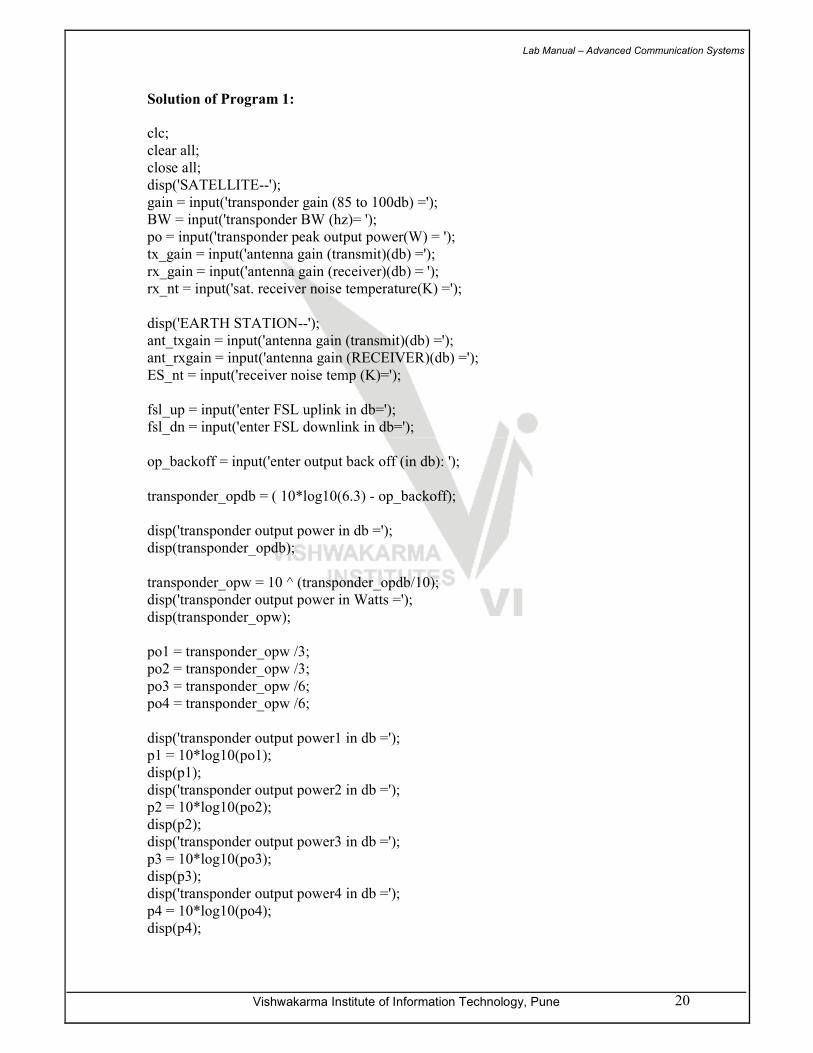
Solution of Program 1:
clc;
clear all;
close all;
disp('SATELLITE--');
gain = input('transponder gain (85 to 100db) =');
BW = input('transponder BW (hz)= ');
po = input('transponder peak output power(W) = ');
tx_gain = input('antenna gain (transmit)(db) =');
rx_gain = input('antenna gain (receiver)(db) = ');
rx_nt = input('sat. receiver noise temperature(K) =');
disp('EARTH STATION--');
ant_txgain = input('antenna gain (transmit)(db) =');
ant_rxgain = input('antenna gain (RECEIVER)(db) =');
ES_nt = input('receiver noise temp (K)=');
fsl_up = input('enter FSL uplink in db=');
fsl_dn = input('enter FSL downlink in db=');
op_backoff = input('enter output back off (in db): ');
transponder_opdb = ( 10*log10(6.3) - op_backoff);
disp('transponder output power in db =');
disp(transponder_opdb);
transponder_opw = 10 ^ (transponder_opdb/10);
disp('transponder output power in Watts =');
disp(transponder_opw);
po1 = transponder_opw /3;
po2 = transponder_opw /3;
po3 = transponder_opw /6;
po4 = transponder_opw /6;
disp('transponder output power1 in db =');
p1 = 10*log10(po1);
disp(p1);
disp('transponder output power2 in db =');
p2 = 10*log10(po2);
disp(p2);
disp('transponder output power3 in db =');
p3 = 10*log10(po3);
disp(p3);
disp('transponder output power4 in db =');
p4 = 10*log10(po4);
disp(p4);
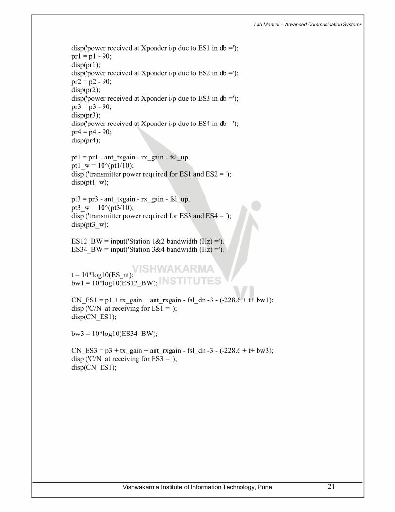
Lab Manual – Advanced Communication Systems
Vishwakarma Institute of Information Technology, Pune 21
disp('power received at Xponder i/p due to ES1 in db =');
pr1 = p1 - 90;
disp(pr1);
disp('power received at Xponder i/p due to ES2 in db =');
pr2 = p2 - 90;
disp(pr2);
disp('power received at Xponder i/p due to ES3 in db =');
pr3 = p3 - 90;
disp(pr3);
disp('power received at Xponder i/p due to ES4 in db =');
pr4 = p4 - 90;
disp(pr4);
pt1 = pr1 - ant_txgain - rx_gain - fsl_up;
pt1_w = 10^(pt1/10);
disp ('transmitter power required for ES1 and ES2 = ');
disp(pt1_w);
pt3 = pr3 - ant_txgain - rx_gain - fsl_up;
pt3_w = 10^(pt3/10);
disp ('transmitter power required for ES3 and ES4 = ');
disp(pt3_w);
ES12_BW = input('Station 1&2 bandwidth (Hz) =');
ES34_BW = input('Station 3&4 bandwidth (Hz) =');
t = 10*log10(ES_nt);
bw1 = 10*log10(ES12_BW);
CN_ES1 = p1 + tx_gain + ant_rxgain - fsl_dn -3 - (-228.6 + t+ bw1);
disp ('C/N at receiving for ES1 = ');
disp(CN_ES1);
bw3 = 10*log10(ES34_BW);
CN_ES3 = p3 + tx_gain + ant_rxgain - fsl_dn -3 - (-228.6 + t+ bw3);
disp ('C/N at receiving for ES3 = ');
disp(CN_ES1);
Lab Manual – Advanced Communication Systems
Vishwakarma Institute of Information Technology, Pune 22
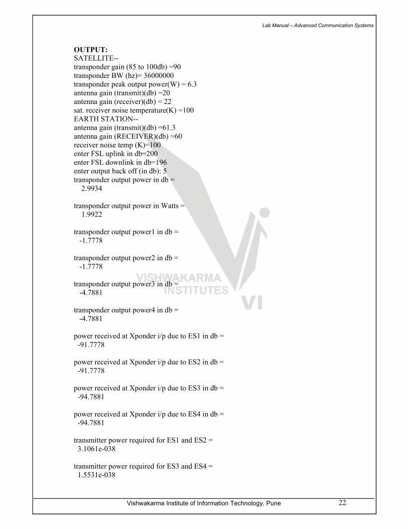
OUTPUT: SATELLITE--
transponder gain (85 to 100db) =90
transponder BW (hz)= 36000000
transponder peak output power(W) = 6.3
antenna gain (transmit)(db) =20
antenna gain (receiver)(db) = 22
sat. receiver noise temperature(K) =100
EARTH STATION--
antenna gain (transmit)(db) =61.3
antenna gain (RECEIVER)(db) =60
receiver noise temp (K)=100
enter FSL uplink in db=200
enter FSL downlink in db=196
enter output back off (in db): 5
transponder output power in db =
2.9934
transponder output power in Watts =
1.9922
transponder output power1 in db =
-1.7778
transponder output power2 in db =
-1.7778
transponder output power3 in db =
-4.7881
transponder output power4 in db =
-4.7881
power received at Xponder i/p due to ES1 in db =
-91.7778
power received at Xponder i/p due to ES2 in db =
-91.7778
power received at Xponder i/p due to ES3 in db =
-94.7881
power received at Xponder i/p due to ES4 in db =
-94.7881
transmitter power required for ES1 and ES2 =
3.1061e-038
transmitter power required for ES3 and ES4 =
1.5531e-038
Lab Manual – Advanced Communication Systems
Vishwakarma Institute of Information Technology, Pune 23
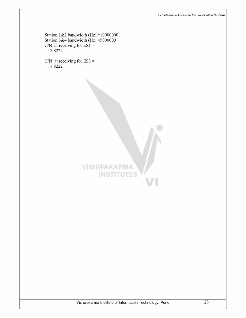
Station 1&2 bandwidth (Hz) =10000000
Station 3&4 bandwidth (Hz) =5000000
C/N at receiving for ES1 =
17.8222
C/N at receiving for ES3 =
17.8222

Lab Manual – Advanced Communication Systems
Vishwakarma Institute of Information Technology, Pune 24
Solution of Program 2:
clc;
close all;
clear all;
uplinkfreq=30e9;
downlinkfreq=42e9;
diameter_rx_ant=0.8;
efficiency_rx_ant=0.6;
beamwidth=1;
NF=7;
To=290;
Latm=1;
Lrain=10;
L_ant_radome=1;
L_contour=3;
L_pointing_error=1.98;
wavelength_up=3e8/downlinkfreq;
ans=(pi*diameter_rx_ant)/wavelength_up;
ans=power(ans,2);
ans=efficiency_rx_ant*ans;
Gr=10*log10(ans);
ans=NF/10;
ans=power(10,ans);
T=To*(ans-1);
T=10*log10(T);
ans=Gr-T;
disp('G/T of receiving station is ');
disp(ans);
P_sat_tx=1;
P_sat_tx=10*log10(P_sat_tx);
IF_BW=30e6;
ans=33000/(beamwidth*beamwidth);
Gt=10*log10(ans);
ans=(4*pi*38000000)/wavelength_up;
ans=power(ans,2);
FSL=10*log10(ans);
k=-228.6;
IF_BW=10*log10(IF_BW);
ans=P_sat_tx+Gt+Gr-FSL-k-T-IF_BW;
disp('C/N of Rx without extra losses');
disp(ans);
ans=P_sat_tx+Gt+Gr-FSL-Latm-Lrain-L_ant_radome-L_contour-L_pointing_error-k-T-
IF_BW;
disp('C/N of Rx');
disp(ans);
ans=13-(Gt+Gr-FSL-Latm-Lrain-L_ant_radome-L_contour-L_pointing_error-k-T-
IF_BW);
ans=ans/10;
Lab Manual – Advanced Communication Systems
Vishwakarma Institute of Information Technology, Pune 25
ans=power(10,ans);
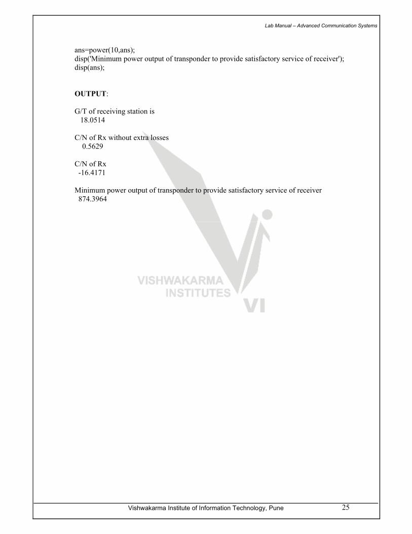
disp('Minimum power output of transponder to provide satisfactory service of receiver');
disp(ans);
OUTPUT:
G/T of receiving station is
18.0514
C/N of Rx without extra losses
0.5629
C/N of Rx
-16.4171
Minimum power output of transponder to provide satisfactory service of receiver
874.3964
Lab Manual – Advanced Communication Systems
Vishwakarma Institute of Information Technology, Pune 26
Solution of Program 3:
clc;
clear all;
close all;
freq_uplink=14.9*(10^9);
freq_downlink=11.3*(10^9);
zone_3db_d1=3.6;
zone_3db_d2=2.4;
ant_eff=0.65;
sat_pow=20;
trans_noise_temp=520;
trans_gain=125; %in db
trans_bw=5*(10^6);
R_km=39000; %in km
R_m=39000000;
pointing_acc_loss=0.5; %in db
%****************************************************
%**Dimensions of transmitting antenna**
wavelenght_down=[3*10^8]/freq_downlink;
dim_trans_1=75*wavelenght_down/zone_3db_d1
dim_trans_2=75*wavelenght_down/zone_3db_d2
%**Dimensions of receiving antenna**
wavelenght_up=[3*10^8]/freq_uplink;
dim_rec_1=75*wavelenght_up/zone_3db_d1
dim_rec_2=75*wavelenght_up/zone_3db_d2
%**Transmitting antenna gain
Gt=ant_eff*4*pi*dim_trans_1*dim_trans_2/(wavelenght_down)^2;
Gt_db=10*log10(Gt)
%**Receiving antenna gain
Gr=ant_eff*4*pi*dim_rec_1*dim_rec_2/(wavelenght_up)^2;
Gr_db=10*log10(Gr)
%*************************************************
%power flux density
flux_den=sat_pow*Gt/(4*pi*R_m^2); %in watts/m2
flux_den_db=10*log10(flux_den)
%flux density at the edge of coverage area
flux_edge=flux_den_db-3
%*************************************************
c_n1=22 ; %indb
Lab Manual – Advanced Communication Systems
Vishwakarma Institute of Information Technology, Pune 27
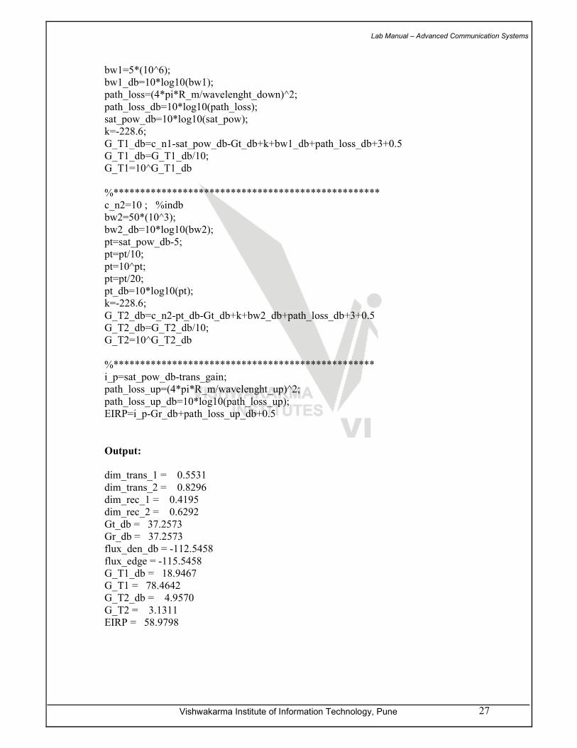
bw1=5*(10^6);
bw1_db=10*log10(bw1);
path_loss=(4*pi*R_m/wavelenght_down)^2;
path_loss_db=10*log10(path_loss);
sat_pow_db=10*log10(sat_pow);
k=-228.6;
G_T1_db=c_n1-sat_pow_db-Gt_db+k+bw1_db+path_loss_db+3+0.5
G_T1_db=G_T1_db/10;
G_T1=10^G_T1_db
%**************************************************
c_n2=10 ; %indb
bw2=50*(10^3);
bw2_db=10*log10(bw2);
pt=sat_pow_db-5;
pt=pt/10;
pt=10^pt;
pt=pt/20;
pt_db=10*log10(pt);
k=-228.6;
G_T2_db=c_n2-pt_db-Gt_db+k+bw2_db+path_loss_db+3+0.5
G_T2_db=G_T2_db/10;
G_T2=10^G_T2_db
%*************************************************
i_p=sat_pow_db-trans_gain;
path_loss_up=(4*pi*R_m/wavelenght_up)^2;
path_loss_up_db=10*log10(path_loss_up);
EIRP=i_p-Gr_db+path_loss_up_db+0.5
Output:
dim_trans_1 = 0.5531
dim_trans_2 = 0.8296
dim_rec_1 = 0.4195
dim_rec_2 = 0.6292
Gt_db = 37.2573
Gr_db = 37.2573
flux_den_db = -112.5458
flux_edge = -115.5458
G_T1_db = 18.9467
G_T1 = 78.4642
G_T2_db = 4.9570
G_T2 = 3.1311
EIRP = 58.9798
Lab Manual – Advanced Communication Systems
Vishwakarma Institute of Information Technology, Pune 28
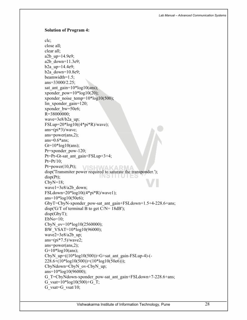
Solution of Program 4:
clc;
close all;
clear all;
a2b_up=14.9e9;
a2b_down=11.3e9;
b2a_up=14.4e9;
b2a_down=10.8e9;
beamwidth=1.5;
ans=33000/2.25;
sat_ant_gain=10*log10(ans);
xponder_pow=10*log10(20);
xponder_noise_temp=10*log10(500);
lin_xponder_gain=120;
xponder_bw=50e6;
R=38000000;
wave=3e8/b2a_up;
FSLup=20*log10((4*pi*R)/wave);
ans=(pi*3)/wave;
ans=power(ans,2);
ans=0.6*ans;
Gt=10*log10(ans);
Pr=xponder_pow-120;
Pt=Pr-Gt-sat_ant_gain+FSLup+3+4;
Pt=Pt/10;
Pt=power(10,Pt);
disp('Transmiter power required to saturate the transponder.');
disp(Pt);
CbyN=18;
wave1=3e8/a2b_down;
FSLdown=20*log10((4*pi*R)/wave1);
ans=10*log10(50e6);
GbyT=CbyN-xponder_pow-sat_ant_gain+FSLdown+1.5+4-228.6+ans;
disp('G/T of terminal B to get C/N= 18dB');
disp(GbyT);
EbNo=10;
CbyN_ov=10*log10(2560000);
BW_VSAT=10*log10(96000);
wave2=3e8/a2b_up;
ans=(pi*7.5)/wave2;
ans=power(ans,2);
G=10*log10(ans);
CbyN_up=((10*log10(500))+G+sat_ant_gain-FSLup-4)-(-
228.6+(10*log10(500))+(10*log10(50e6)));
CbyNdown=CbyN_ov-CbyN_up;
ans=10*log10(96000);
G_T=CbyNdown-xponder_pow-sat_ant_gain+FSLdown+7-228.6+ans;
G_vsat=10*log10(500)+G_T;
G_vsat=G_vsat/10;
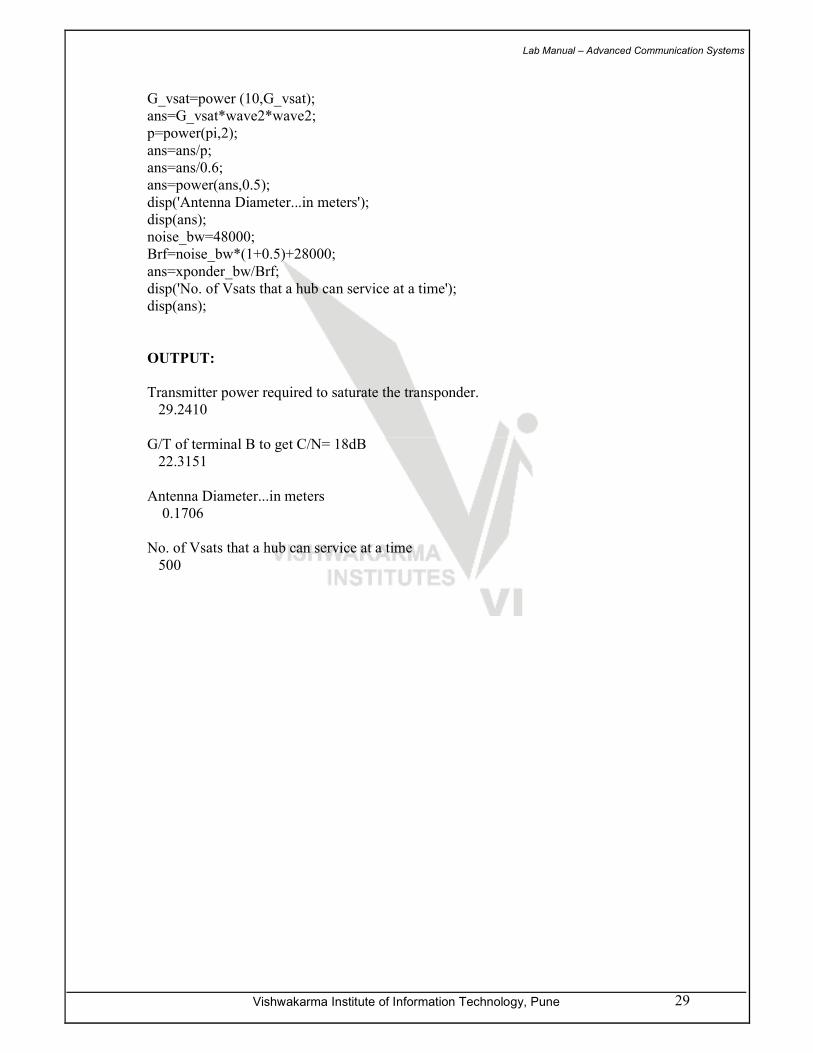
Lab Manual – Advanced Communication Systems
Vishwakarma Institute of Information Technology, Pune 29
G_vsat=power (10,G_vsat);
ans=G_vsat*wave2*wave2;
p=power(pi,2);
ans=ans/p;
ans=ans/0.6;
ans=power(ans,0.5);
disp('Antenna Diameter...in meters');
disp(ans);
noise_bw=48000;
Brf=noise_bw*(1+0.5)+28000;
ans=xponder_bw/Brf;
disp('No. of Vsats that a hub can service at a time');
disp(ans);
OUTPUT:
Transmitter power required to saturate the transponder.
29.2410
G/T of terminal B to get C/N= 18dB
22.3151
Antenna Diameter...in meters
0.1706
No. of Vsats that a hub can service at a time
500
Lab Manual – Advanced Communication Systems
Vishwakarma Institute of Information Technology, Pune 30
EXPERIMENT NO: 05
TITLE OF EXPERIMENT : To Study of Wavelength Division
Multiplexing

Lab Manual – Advanced Communication Systems
Vishwakarma Institute of Information Technology, Pune 31
5.1 Aim: To Study of Wavelength Division Multiplexing.
5.2 Objective:
1. Study of the Multiplexing & De-multiplexing of two different signal using Laser Diode (At
1310 nm and 1550 nm) and Photo detector.
2. Observe the waveform at Multiplex output and DE- Multiplex output
5.3 Apparatus: NWS _1310nm_LTK board + NWS_1310nm_TX-RX board. (Box -1)
NWS_1550nm_LTK board + NWS_1550nm_TX-RX board. (Box - 2)
Optical Multiplexer, De-multiplexer, ST to ST Coupler, Connecting Cable with Spin connector on
either side, CRO/DSO, Power Supply, etc.
5.4 Procedure:
1. Make the all jumper settings of Analog link on the NWS_1310nm_LTK &
NWS_1310nm_TX-RX (Box -1)
2. Make the all jumper settings of Digital link on the NWS_1550nm_LTK &
NWS_1310nm_TX-RX (Box -2)
3. Optical Mux and De-Mux provided with the kits are interchangeable. Each of them
consists of two single mode fiber cables connected at one end carrying separate
wavelengths and one single mode fiber cable at other end carrying multiplexed
wavelengths. These cables are terminated at one end by ST connectors. Cable marked as
1310 carries 1310 nm wavelength and that marked as 1550 carries 1550 nm wavelength due
to the internal arrangements with the MUX or De-Mux
4. Insert the ST connector of the Mux cable marked as 1310 in to the ST housing of the
1310nm LASER and ST connector of MUX cable marked as 1550 in to the ST housing of
the 1550nm LASER and lock it properly
5. Connect the ST coupler provided with the kit between the single cables of Mux & De-mux.
This will couple the Mux and De-Mux to each other
6. Insert the ST connector of the De-Mux cable marked as 1310 in to the ST housing of the
Photo detector (D1) on NWS_1310nm_TX-RX board. Similarly Insert the ST connector of
the De-Mux cable marked as 1550 in to the ST housing of the Photo detector (D1) on
NWS_1550nm_TX-RX board
7. Switch ON the power supply & press the switch SW 1 on each of the Box to power the
Laser drivers & Lasers with delay
8. Note that since 1310 nm Laser is configured to transmit analog signal and 1550 nm Laser is
configured to transmit digital signal, optical MUX will multiplex these two different signals
and transmit them simultaneously through single fiber cable at the output. The De-MUX
will de-multiplex these two wavelengths (Thus signals) in to separate channels at its
output
9. You can observe the recovered signals at the receiver output. You will recover both analog
as well as digital signals

Lab Manual – Advanced Communication Systems
Vishwakarma Institute of Information Technology, Pune 32
10. This proves that by optical multiplexing two different wavelengths carrying different
signals (Information) we can increase the signal carrying capacity of the fiber cable to a
large extent
5.5 Conclusion: _____________________________________________________
_____________________________________________________
_____________________________________________________
_____________________________________________________
Lab Manual – Advanced Communication Systems
Vishwakarma Institute of Information Technology, Pune 33
EXPERIMENT NO: 06
TITLE OF EXPERIMENT : To prepare Optical Link Power Budget
for Repeater less Optical Fiber Link using
MATLAB & Microsoft Excel
Lab Manual – Advanced Communication Systems
Vishwakarma Institute of Information Technology, Pune 34
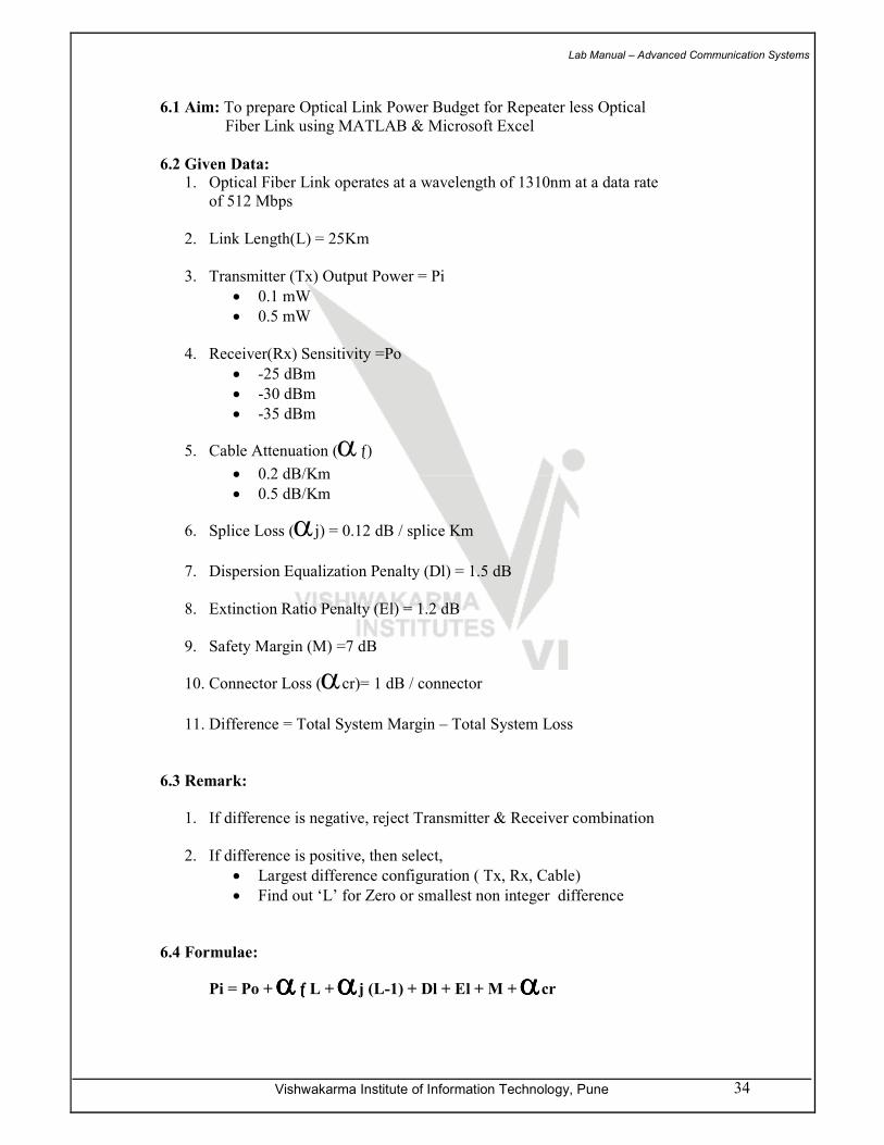
6.1 Aim: To prepare Optical Link Power Budget for Repeater less Optical
Fiber Link using MATLAB & Microsoft Excel
6.2 Given Data:
1. Optical Fiber Link operates at a wavelength of 1310nm at a data rate
of 512 Mbps
2. Link Length(L) = 25Km
3. Transmitter (Tx) Output Power = Pi
• 0.1 mW
• 0.5 mW
4. Receiver(Rx) Sensitivity =Po
• -25 dBm
• -30 dBm
• -35 dBm
5. Cable Attenuation (αƒ)
• 0.2 dB/Km
• 0.5 dB/Km
6. Splice Loss (αj) = 0.12 dB / splice Km
7. Dispersion Equalization Penalty (Dl) = 1.5 dB
8. Extinction Ratio Penalty (El) = 1.2 dB
9. Safety Margin (M) =7 dB
10. Connector Loss (αcr)= 1 dB / connector
11. Difference = Total System Margin – Total System Loss
6.3 Remark:
1. If difference is negative, reject Transmitter & Receiver combination
2. If difference is positive, then select,
• Largest difference configuration ( Tx, Rx, Cable)
• Find out ‘L’ for Zero or smallest non integer difference
6.4 Formulae:
Pi = Po + αααჃƒƒ L + ααααj (L-1) + Dl + El + M + ααααcr
Lab Manual – Advanced Communication Systems
Vishwakarma Institute of Information Technology, Pune 35
6.5 Calculations: 1. using MATLAB
2. using Microsoft Excel
Note: Attach Graphs using both the methods
6.6 Conclusion: _____________________________________________________
_____________________________________________________
_____________________________________________________
_____________________________________________________
Lab Manual – Advanced Communication Systems
Vishwakarma Institute of Information Technology, Pune 36
EXPERIMENT NO: 07
TITLE OF EXPERIMENT : Displacement Measurement using Optical
sensors
Lab Manual – Advanced Communication Systems
Vishwakarma Institute of Information Technology, Pune 37
7.1 Aim: To study working and characteristics of fiber optic displacement transducer
7.2 Apparatus: Optical Transmitter and Receiver Box, fiber cable, micrometer, digital
multimeter, LVDT Kit, etc
7.3 Theory:
7.3.1 Fiber optic sensors Optical fibers can be used as sensors to measure strain, temperature, pressure,
displacement and other parameters. The small size and the fact that no electrical power is
needed at the remote location give the fiber optic sensor advantages to conventional
electrical sensor in certain applications.
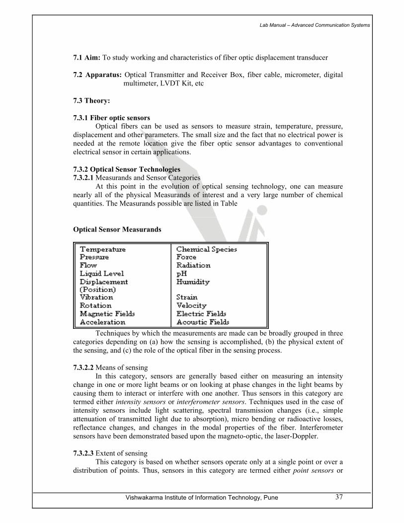
7.3.2 Optical Sensor Technologies
7.3.2.1 Measurands and Sensor Categories
At this point in the evolution of optical sensing technology, one can measure
nearly all of the physical Measurands of interest and a very large number of chemical
quantities. The Measurands possible are listed in Table
Optical Sensor Measurands
Techniques by which the measurements are made can be broadly grouped in three
categories depending on (a) how the sensing is accomplished, (b) the physical extent of
the sensing, and (c) the role of the optical fiber in the sensing process.
7.3.2.2 Means of sensing
In this category, sensors are generally based either on measuring an intensity
change in one or more light beams or on looking at phase changes in the light beams by
causing them to interact or interfere with one another. Thus sensors in this category are termed either intensity sensors or interferometer sensors. Techniques used in the case of
intensity sensors include light scattering, spectral transmission changes (i.e., simple
attenuation of transmitted light due to absorption), micro bending or radioactive losses,
reflectance changes, and changes in the modal properties of the fiber. Interferometer
sensors have been demonstrated based upon the magneto-optic, the laser-Doppler.
7.3.2.3 Extent of sensing
This category is based on whether sensors operate only at a single point or over a
distribution of points. Thus, sensors in this category are termed either point sensors or
Lab Manual – Advanced Communication Systems
Vishwakarma Institute of Information Technology, Pune 38
distributed sensors. In the case of a point sensor, the transducer may be at the end of a
fiber the sole purpose of which is to bring a light beam to and from the transducer.
7.3.2.4 Role of optical fiber
Further distinction is often made in the case of fiber sensors as to whether
Measurands act externally or internally to the fiber. Where the transducers are external to
the fiber and the fiber merely registers and transmits the sensed quantity, the sensors are
termed extrinsic sensors. Where the sensors are embedded in or are part of the fiber -- and
for this type there is often some modification to the fiber itself -- the sensors are termed
internal or intrinsic sensors. Examples of extrinsic sensors are moving gratings to sense
strain, fiber-to-fiber couplers to sense displacement, and absorption cells to sense
chemistry effects. Examples of intrinsic sensors are those that use micro bending losses in
the fiber to sense strain, modified fiber claddings to make spectroscopic measurements,
and counter-propagating beams within a fiber coil to measure rotation.
7.3.2.5 Displacement and position sensors
The simplest sensors rely on the change in retro reflectance of light into a fiber
because of movement of a proximal mirror surface. One of the first Photonics sensors was
of this type, in which a conical tip is applied to the end of a fiber. Light is totally reflected
back into the fiber if the surrounding medium is air; however, if the fiber is inserted into a
liquid matching the fiber index, light is extracted from the fiber and lost. Thus,
displacement of the liquid surface can be tracked.
7.3.3 Enabling Sensor Components
7.3.3.1 Specialty fibers for sensors
Since a large percentage of today's optical sensors involve optical fibers in some
form, it is important to discuss the status of fiber R&D. For much of the work, sensor
designers have made use of the all-glass fibers that are readily available commercially
due to high-volume use in telecommunications. Interferometer sensors need single-mode,
all-glass fibers; intensity type sensors typically utilize multimode fiber for greater light-
gathering capability. While high-NA (numerical aperture) plastic fibers are used for some
intensity type sensors, the transmission and fluorescence properties of the plastic
complicate the spectral response, so all-glass fibers are favored for many spectroscopic-
type sensors. Polarized light transmission is important for a number of sensors (e.g., the
fiber-optic gyroscope, FOG); many fiber devices are designed to retain this property
along the length of the fiber and in the presence of macro- and micro-bending. In the case
of the FOG, the requirements are for a small coil of fiber for which the bending loss must
be small, the polarization properties of the light must be maintained, and the physical
strength of the fiber must not be jeopardized. For many of the chemical sensors, it is
important for the light wave to interact with its surroundings. Therefore, fibers have been
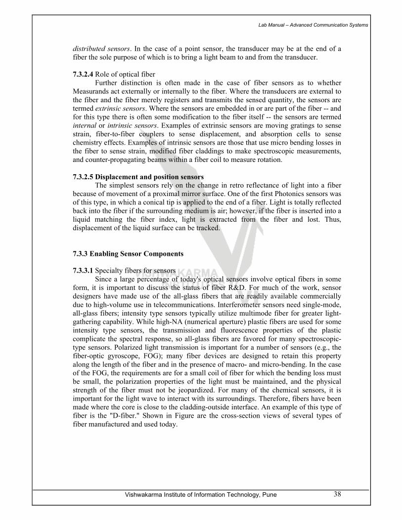
made where the core is close to the cladding-outside interface. An example of this type of
fiber is the "D-fiber." Shown in Figure are the cross-section views of several types of
fiber manufactured and used today.
Lab Manual – Advanced Communication Systems
Vishwakarma Institute of Information Technology, Pune 39
Fig. End view of specialty fibers.
7.3.3.2 Detectors
While not much change has taken place in the semiconductor devices actually
used to convert photons into electrons, progress continues to be made in readout
techniques for the sensor signals. Of particular note is the use of optical fiber
interferometers to monitor other interferometer sensors.
7.3.3.3 Light sources The majority of optical sensors still utilize semiconductor lasers and LEDs as light
sources. Increasingly, however, the low-cost semiconductor lasers have been used to
pump rare-earth-doped fibers to provide excellent, stable fluorescent sources for chemical
monitoring.
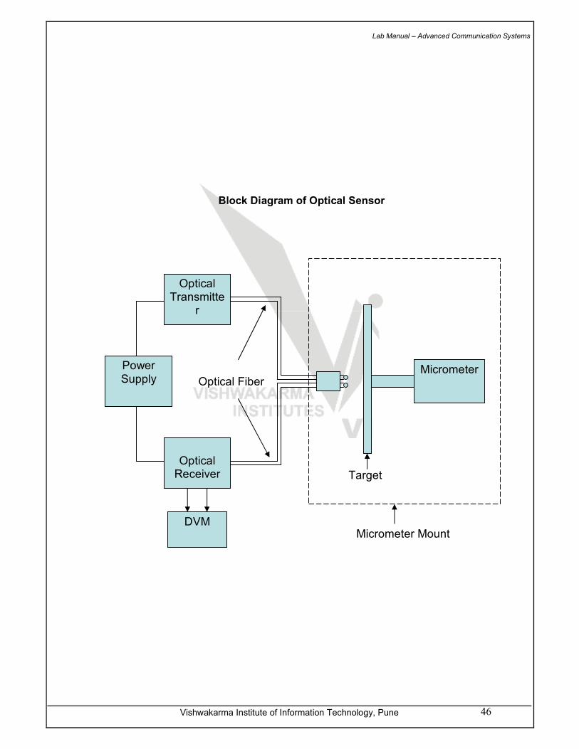
7.4 Procedure:
1. Connect power cord to the transmitter box and Receiver Box, and then switch ON
the power supply.
2. Insert the fiber optic cable from transmitter to LVDT kit
3. Insert other fiber optic cable from LVDT to Receiver Box.
4. Attach DVM at the output of the Receiver
5. Move the LVDT using micrometer; i.e. assembly attached with the LVDT kit
6. Measure the DC output voltage and plot the graph of displacement vs. DC output
voltage
7.5 Observation table:
Sr. No. Displacement
(mm)
Dc output voltage
(V)
1
2
3
7.6 Conclusion: _____________________________________________________
_____________________________________________________
_____________________________________________________
_____________________________________________________
Lab Manual – Advanced Communication Systems
Vishwakarma Institute of Information Technology, Pune 40
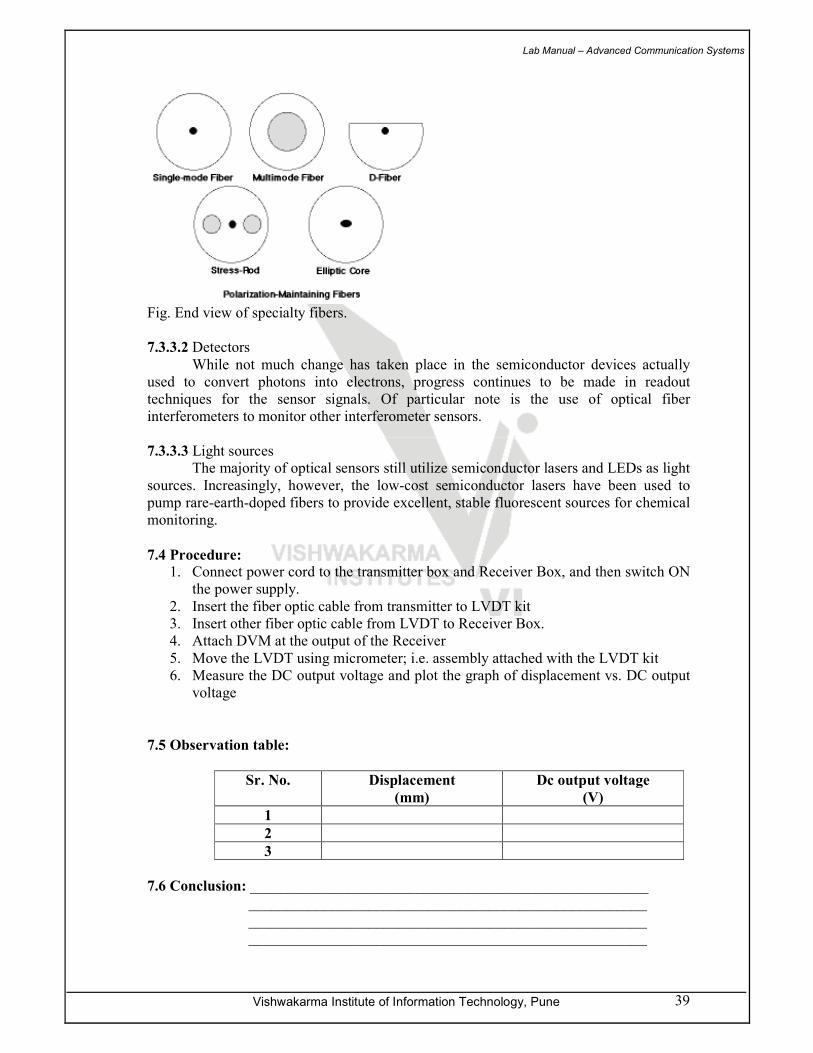
Isolator
Klystron Oscillator
Attenuator
Klystron Power Supply
Frequency Meter
Fig. Horn Antenna Bench Setup
Detector
CRO

Lab Manual – Advanced Communication Systems
Vishwakarma Institute of Information Technology, Pune 41
Block Diagram of WDM:
Laser (D1) 1310nm
Laser (D2) 1550nm
Multiplexer Power Supply
De- Multiplexer
1310nm Photo Detector
1550nm Photo Detector
CRO
Analog Signal
Digital Signal
ST to ST Coupler
Lab Manual – Advanced Communication Systems
Vishwakarma Institute of Information Technology, Pune 42
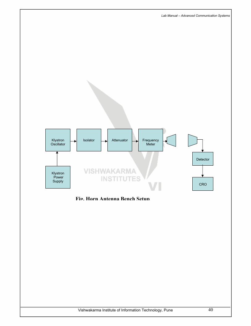
• Connect Ammeter cable to J2 with White dot of connector on right while facing back side of it to you. Keep J3 (Digital_CON), J4 (ANALOG_CON), J7 (TDM_CON) open.
• Similarly, keep jumpers J2 (ANALOG/DIGITAL SEL), J3 (TDM_RX / RS 232 SEL), J8 (TDM_OUT_CON) open & connectors J4 (DIGITAL CON), J6 (PCI) & J7 (PC3) unconnected on NWS_131 Onm_TX_RX board.
Analog Jumper setting
1 2 3 4
1 2 3
A/D SEL
1 2
MOD_CON
LASER CON
J2
J5
J6
1 2 3 4
SW2
ON
EXT_IN W
J5
Signal I/P
Amp I/P
MIC M/P
On NWS_1310nm_Tx_Rx board
Analog Con
Lab Manual – Advanced Communication Systems
Vishwakarma Institute of Information Technology, Pune 43
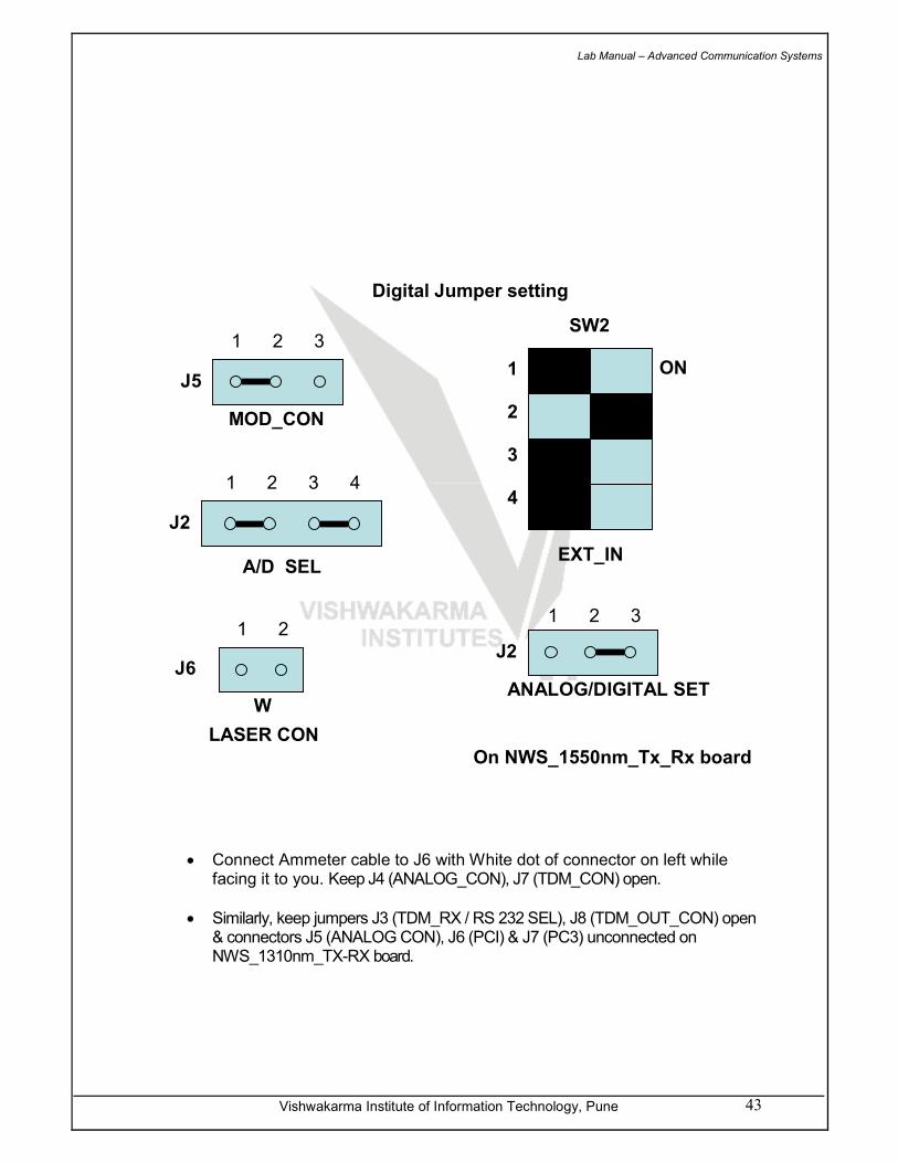
• Connect Ammeter cable to J6 with White dot of connector on left while facing it to you. Keep J4 (ANALOG_CON), J7 (TDM_CON) open.
• Similarly, keep jumpers J3 (TDM_RX / RS 232 SEL), J8 (TDM_OUT_CON) open & connectors J5 (ANALOG CON), J6 (PCI) & J7 (PC3) unconnected on NWS_1310nm_TX-RX board.
Digital Jumper setting
1 2 3
MOD_CON
J5
1 2 3 4
A/D SEL
J2
1 2
LASER CON
1 2 3 4
ON
EXT_IN
ANALOG/DIGITAL SET
J2
1 2 3
On NWS_1550nm_Tx_Rx board
J6
SW2
W

Lab Manual – Advanced Communication Systems
Vishwakarma Institute of Information Technology, Pune 44
Block Diagram of Satellite System
Satellite
Uplink Transmitter
Satellite
downlink Receiver
Satellite
Link Emulator
CROVideo
Monitor
Spectrum
Analyzer
Function
GeneratorCRO
Lab Manual – Advanced Communication Systems
Vishwakarma Institute of Information Technology, Pune 45
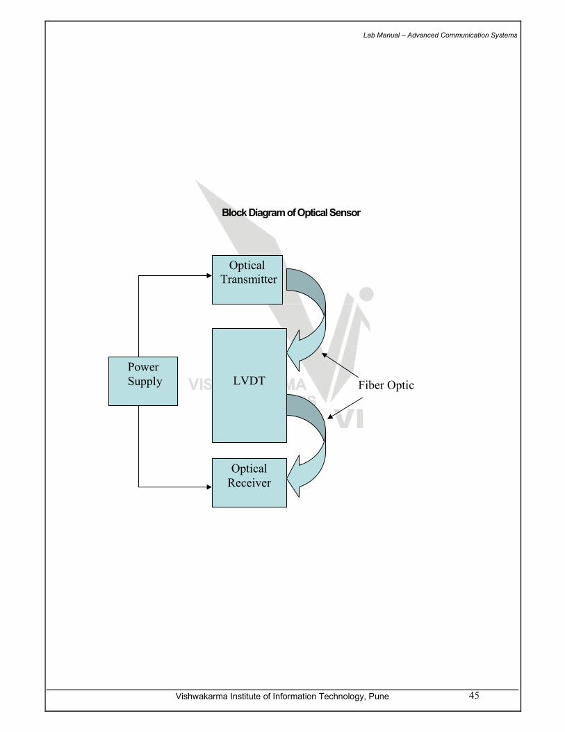
Block Diagram of Optical Sensor
Power
Supply
LVDT
Optical
Transmitter
Optical
Receiver
Fiber Optic
Lab Manual – Advanced Communication Systems
Vishwakarma Institute of Information Technology, Pune 46
Power Supply
DVM
Optical Receiver
Optical Transmitte
r
Micrometer
Target
Micrometer Mount
Optical Fiber
Block Diagram of Optical Sensor