ACTA UNIVERSITATIS UPSALIENSIS Uppsala Dissertations from the Faculty of Science and Technology

131

Kaj Jansson

Measurements of Neutron-induced Nuclear Reactions for More Precise Standard Cross Sections and Correlated Fission Properties

Dissertation presented at Uppsala University to be publicly examined in Polhemsalen,Ångströmlaboratoriet, Lägerhyddsvägen 1, Uppsala, Friday, 10 November 2017 at 09:15 forthe degree of Doctor of Philosophy. The examination will be conducted in English. Facultyexaminer: Fanny Farget (CNRS/IN2P3).

AbstractJansson, K. 2017. Measurements of Neutron-induced Nuclear Reactions for More PreciseStandard Cross Sections and Correlated Fission Properties. Uppsala Dissertations from theFaculty of Science and Technology 131. 142 pp. Uppsala: Acta Universitatis Upsaliensis.ISBN 978-91-513-0085-6.

It is difficult to underestimate the importance of neutron cross section standards in the nucleardata field. Accurate and precise standards are prerequisites for measuring neutron cross sections.Two different projects are presented here with the aim of improving on neutron standards.

A simulation study was performed for an experiment intended to measure the cross sections ofH(n,n), 235U(n,f), and 238U(n,f) relative to each other. It gave the first estimates of the performanceof the experimental setup. Its results have aided the development of the experimental setup bysetting limits on the target and detector design.

A second neutron-standard project resulted in three measurements of 6Li(n,α)t relative to235U(n,f). Each subsequent measurement improved upon the previous one and changed theexperimental setup accordingly. Although, preliminary cross sections were agreeing well withevaluated data files in some energy intervals, the main goal to measure the cross section up to3 MeV was not reached.

Mass yields and energy spectra are important outcomes of many fission experiments, but inlow yield regions the uncertainties are still high even for recurrently studied nuclei. In order tounderstand the fission dynamics, one also needs correlated fission data. One particular importantproperty is the distribution of excitation energy between the two nascent fission fragments. Itis closely connected to the prompt emission of neutrons and γ’s and reveals information abouthow nucleons and energy are transferred within the fissioning nucleus.

By measuring both the pre and post neutron-emission fragment masses, the cumbrance ofdetecting neutrons directly is overcome. This is done using the fission spectrometer VERDI andthe 2E-2v method. In this work I describe how both the spectrometer, the analysis method, andthe calibration procedures have been further developed. Preliminary experimental data show thegreat potential of VERDI, but also areas that call for more attention. A previously overlookedconsequence of a central assumption was found and a correction method is proposed that cancorrect previously obtained data as well.

The last part of this thesis concerns the efficiencies of the fission product extraction at theIGISOL facility. The methodology of the fission yield measurements at IGISOL are reliant onassumptions that have not been systematically investigated. The presented work is a first step ofsuch an investigation that can also be used as a tool for optimising the setup for measurementsof exotic nuclei. A simulation framework connecting three different simulation codes wasdeveloped to investigate the produced yield of fission products in a buffer gas. Several differentvariants of the setup were simulated and the findings were generally accordant with previousestimates. A reasonable agreement between experimental data and the simulation results isdemonstrated.

Keywords: Cross Section, Fission, Neutron-induced reactions, Simulation, VERDI

Kaj Jansson, Department of Physics and Astronomy, Applied Nuclear Physics, Box 516,Uppsala University, SE-751 20 Uppsala, Sweden.

© Kaj Jansson 2017

ISSN 1104-2516ISBN 978-91-513-0085-6urn:nbn:se:uu:diva-329953 (http://urn.kb.se/resolve?urn=urn:nbn:se:uu:diva-329953)

Contents

1 Introduction 11.1 Thesis outline . . . . . . . . . . . . . . . . . . . . . . . . . . 21.2 Reuse of previous work . . . . . . . . . . . . . . . . . . . . . 2

2 Neutron-induced nuclear reactions 32.1 Neutron standard cross sections . . . . . . . . . . . . . . . . . 3

2.1.1 Relative measurements . . . . . . . . . . . . . . . . . . 52.2 Nuclear structure . . . . . . . . . . . . . . . . . . . . . . . . . 52.3 Compound reactions . . . . . . . . . . . . . . . . . . . . . . . 62.4 Fission . . . . . . . . . . . . . . . . . . . . . . . . . . . . . . 8

3 Particle detectors 153.1 Frisch-gridded ionisation chambers . . . . . . . . . . . . . . . 16

3.1.1 Obtaining angular information . . . . . . . . . . . . . . 163.1.2 Loss of charge and choice of gas . . . . . . . . . . . . . 20

3.2 Parallel plate avalanche counters . . . . . . . . . . . . . . . . 213.3 Multi-channel plates . . . . . . . . . . . . . . . . . . . . . . . 223.4 Silicon detectors . . . . . . . . . . . . . . . . . . . . . . . . . 23

3.4.1 Radiation damage . . . . . . . . . . . . . . . . . . . . 243.4.2 Detecting heavy ions in silicon detectors . . . . . . . . 25

4 Neutron facilities 274.1 NFS . . . . . . . . . . . . . . . . . . . . . . . . . . . . . . . 274.2 GELINA . . . . . . . . . . . . . . . . . . . . . . . . . . . . . 284.3 IGISOL . . . . . . . . . . . . . . . . . . . . . . . . . . . . . 28

5 Neutron standards at NFS 305.1 Motivation . . . . . . . . . . . . . . . . . . . . . . . . . . . . 305.2 Experimental setup . . . . . . . . . . . . . . . . . . . . . . . 32

5.2.1 Detector telescopes . . . . . . . . . . . . . . . . . . . . 345.2.2 Stacked target . . . . . . . . . . . . . . . . . . . . . . . 355.2.3 Neutron energy . . . . . . . . . . . . . . . . . . . . . . 355.2.4 Particle identification . . . . . . . . . . . . . . . . . . . 365.2.5 Observables . . . . . . . . . . . . . . . . . . . . . . . 36

5.3 Simulations . . . . . . . . . . . . . . . . . . . . . . . . . . . 375.3.1 Simulation setup . . . . . . . . . . . . . . . . . . . . . 385.3.2 Simulation results . . . . . . . . . . . . . . . . . . . . 38

5.4 Current status . . . . . . . . . . . . . . . . . . . . . . . . . . 42

v

6 Alpha-particle and triton production at GELINA 436.1 Motivation . . . . . . . . . . . . . . . . . . . . . . . . . . . . 436.2 First experiment . . . . . . . . . . . . . . . . . . . . . . . . . 45

6.2.1 Experimental setup . . . . . . . . . . . . . . . . . . . . 456.2.2 Analysis procedure . . . . . . . . . . . . . . . . . . . . 466.2.3 Results . . . . . . . . . . . . . . . . . . . . . . . . . . 54

6.3 Second experiment . . . . . . . . . . . . . . . . . . . . . . . . 586.3.1 Changes compared to the original experiment . . . . . . 586.3.2 Results . . . . . . . . . . . . . . . . . . . . . . . . . . 59

6.4 Third experiment . . . . . . . . . . . . . . . . . . . . . . . . . 606.4.1 Changes compared to the second experiment . . . . . . 606.4.2 Results . . . . . . . . . . . . . . . . . . . . . . . . . . 63

6.5 Improvements for a next experiment . . . . . . . . . . . . . . . 666.5.1 DAQ . . . . . . . . . . . . . . . . . . . . . . . . . . . 666.5.2 γ-flash . . . . . . . . . . . . . . . . . . . . . . . . . . 666.5.3 The lithium chamber . . . . . . . . . . . . . . . . . . . 67

7 Correlated fission observables with VERDI 687.1 Motivation . . . . . . . . . . . . . . . . . . . . . . . . . . . . 687.2 Notation . . . . . . . . . . . . . . . . . . . . . . . . . . . . . 697.3 The 2E method . . . . . . . . . . . . . . . . . . . . . . . . . . 697.4 The 2E-2v method . . . . . . . . . . . . . . . . . . . . . . . . 70

7.4.1 Isotropic neutron emission . . . . . . . . . . . . . . . . 707.4.2 Pre- and post-neutron masses and energies . . . . . . . 72

7.5 Experimental setup . . . . . . . . . . . . . . . . . . . . . . . 747.6 Simulation study . . . . . . . . . . . . . . . . . . . . . . . . . 767.7 VERDI data analysis . . . . . . . . . . . . . . . . . . . . . . . 79

7.7.1 Time-of-flight calibration . . . . . . . . . . . . . . . . 807.7.2 Energy calibration and PHD corrections . . . . . . . . . 807.7.3 PDT corrections . . . . . . . . . . . . . . . . . . . . . 827.7.4 Comparison of calibration methods . . . . . . . . . . . 887.7.5 Intrinsic deficiency in the 2E-2v method . . . . . . . . 907.7.6 Detection efficiency . . . . . . . . . . . . . . . . . . . 947.7.7 Ternary fission . . . . . . . . . . . . . . . . . . . . . . 98

7.8 The future and unresolved issues . . . . . . . . . . . . . . . . 98

8 Simulated ion stopping at IGISOL 1018.1 Ion guide for proton-induced fission . . . . . . . . . . . . . . . 102

8.1.1 Experimental setup . . . . . . . . . . . . . . . . . . . . 1028.1.2 Simulation setup . . . . . . . . . . . . . . . . . . . . . 1028.1.3 Main results . . . . . . . . . . . . . . . . . . . . . . . 104

8.2 Ion guide for neutron-induced fission . . . . . . . . . . . . . . 1068.2.1 The neutron source . . . . . . . . . . . . . . . . . . . . 1088.2.2 The ion guide . . . . . . . . . . . . . . . . . . . . . . . 109

vi

8.2.3 Ion stopping simulation . . . . . . . . . . . . . . . . . 1118.2.4 Results . . . . . . . . . . . . . . . . . . . . . . . . . . 1128.2.5 Conclusions . . . . . . . . . . . . . . . . . . . . . . . 119

9 Svensk sammanfattning (Summary in Swedish) 121

10 Acknowledgements 124

Appendix A: Code developed . . . . . . . . . . . . . . . . . . . . . . . 126A.1 Modifications to Geant4 . . . . . . . . . . . . . . . . . . . . . 126

A.1.1 Extended and corrected cross sections . . . . . . . . . . 126A.1.2 Biasing of discrete events in simulations . . . . . . . . 127A.1.3 New effective charge model . . . . . . . . . . . . . . . 129

A.2 ROOT file I/O made simple . . . . . . . . . . . . . . . . . . . 130A.3 Acquisition software for a SPdevices digitiser . . . . . . . . . . 131

Appendix B: Selected publications . . . . . . . . . . . . . . . . . . . . 133

References 136

vii

List of Figures

2.1 Prompt radiation. . . . . . . . . . . . . . . . . . . . . . . . . . 92.2 FF excitation energy as a function of mass. . . . . . . . . . . . 102.3 Schematic fission barrier. . . . . . . . . . . . . . . . . . . . . 122.4 TKE as a function of mass. . . . . . . . . . . . . . . . . . . . 143.1 GIC electrodes. . . . . . . . . . . . . . . . . . . . . . . . . . 173.2 GIC signals. . . . . . . . . . . . . . . . . . . . . . . . . . . . 173.3 Prototype PPACs developed in our lab. . . . . . . . . . . . . . 223.4 Detector telescope. . . . . . . . . . . . . . . . . . . . . . . . . 245.1 Fission cross section discrepancies. . . . . . . . . . . . . . . . 315.2 The Medley setup. . . . . . . . . . . . . . . . . . . . . . . . . 335.3 Medley target area. . . . . . . . . . . . . . . . . . . . . . . . . 335.4 Simulated ΔE-ΔE plot. . . . . . . . . . . . . . . . . . . . . . 375.5 Contributions to the neutron energy resolution. . . . . . . . . . 395.6 Expected uncertainty in the incoming neutron energy. . . . . . 405.7 Fraction of FPs below a certain energy threshold. . . . . . . . . 416.1 Resonance structure of the 6Li(n,α)t reaction. . . . . . . . . . 446.2 Schematic of the original ionisation chamber. . . . . . . . . . . 466.3 Anode and grid signals from an α-event. . . . . . . . . . . . . 476.4 Correction of time walk. . . . . . . . . . . . . . . . . . . . . . 496.5 Grid-anode plot of fission events. . . . . . . . . . . . . . . . . 506.6 Energy loss correction for fission events. . . . . . . . . . . . . 516.7 Grid-anode plot of α-particle events. . . . . . . . . . . . . . . 536.8 Cosine distributions of fission events. . . . . . . . . . . . . . . 556.9 Energy spectra for fission events. . . . . . . . . . . . . . . . . 556.10 α-particle events transformed into the CoM frame. . . . . . . . 576.11 Deduced cross section from the first experimental run. . . . . . 576.12 Test of 95% Ar+5% CO2 gas mixture. . . . . . . . . . . . . . . 586.13 Schematic of the split ionisation chamber. . . . . . . . . . . . 616.14 Fitted signals. . . . . . . . . . . . . . . . . . . . . . . . . . . 636.15 Improvements in the cosine distributions. . . . . . . . . . . . . 646.16 Grid-anode plot for α-particle and triton events. . . . . . . . . 646.17 Deduced cross section from the third experimental run. . . . . 657.1 Effects of mass and relativism. . . . . . . . . . . . . . . . . . 737.2 The VERDI setup. . . . . . . . . . . . . . . . . . . . . . . . . 747.3 Photo of one of the MCPs. . . . . . . . . . . . . . . . . . . . . 757.4 Electronic scheme of the VERDI setup. . . . . . . . . . . . . . 777.5 Coincidence rate estimation due to broken collinearity. . . . . . 79

viii

7.6 Different choices of energy calibrations. . . . . . . . . . . . . 827.7 One dimensional distributions when the Velkovska method was

used. . . . . . . . . . . . . . . . . . . . . . . . . . . . . . . . 847.8 The Velkovska method fails. . . . . . . . . . . . . . . . . . . . 847.9 New method to parametrise the PDT. . . . . . . . . . . . . . . 857.10 One dimensional distributions when the new PDT correction

was used. . . . . . . . . . . . . . . . . . . . . . . . . . . . . . 867.11 Testing the new PDT correction method on synthetic data. . . . 877.12 The experimental neutron multiplicity for different analysis

choices. . . . . . . . . . . . . . . . . . . . . . . . . . . . . . . 897.13 Total neutron multiplicity as a function of TKE. . . . . . . . . 897.14 Experimentally derived PDTs. . . . . . . . . . . . . . . . . . . 907.15 Neutron multiplicity derived from synthetic data. . . . . . . . . 917.16 Masswise correlation between Mpre and ν̄. . . . . . . . . . . . 927.17 Standard deviations of the mass broadening. . . . . . . . . . . 947.18 The corrected ν̄(Mpre) from 252Cf(sf ). . . . . . . . . . . . . . 957.19 The corrected ν̄(Mpre) from 235U(nth,f). . . . . . . . . . . . . . 957.20 TKE dependent detection efficiency. . . . . . . . . . . . . . . 967.21 The effect of detection efficiency. . . . . . . . . . . . . . . . . 977.22 Neutron multiplicity dependence on detection efficiency. . . . . 987.23 Ternary particles detected by VERDI. . . . . . . . . . . . . . . 998.1 Neutron- and proton-induced fission yields. . . . . . . . . . . . 1028.2 Setup used for the proton-induced experiment. . . . . . . . . . 1038.3 Chosen FP energies. . . . . . . . . . . . . . . . . . . . . . . . 1048.4 Ion stopping efficiency as a function of mass. . . . . . . . . . . 1058.5 Ion stopping efficiency as a function of kinetic energy. . . . . . 1058.6 Map of where the simulated ions stops. . . . . . . . . . . . . . 1068.7 Dependence on target thickness. . . . . . . . . . . . . . . . . . 1078.8 Dependence on nickel foil thickness. . . . . . . . . . . . . . . 1078.9 The neutron flux on top of a schematic of the ion guide. . . . . 1088.10 3D rendering of the simulated geometry. . . . . . . . . . . . . 1108.11 Cross sectional schematics of the target placements. . . . . . . 1108.12 The average neutron flux, the fission cross section, and the

average fission rate. . . . . . . . . . . . . . . . . . . . . . . . 1128.13 Mass yields of stopped ions from simulation Sim I. . . . . . . 1148.14 Charge yields of stopped ions from simulation Sim I. . . . . . 1148.15 Effects of effective charge model and increased pressure. . . . . 1158.16 Yield of the ions stopped in the gas from Sim I. . . . . . . . . 1178.17 Yield of the ions stopped in the gas from Sim VI. . . . . . . . 1178.18 Positions of the ions stopped in the gas from Sim VII. . . . . . 1188.19 Cumulative distribution of the how far the stopped ions travelled.119A.1 Correction of the elastic neutron scattering cross section. . . . 127

ix

List of Tables

2.1 The IAEA neutron standards. . . . . . . . . . . . . . . . . . . 42.2 The first six magic numbers. . . . . . . . . . . . . . . . . . . . 73.1 GIC notation. . . . . . . . . . . . . . . . . . . . . . . . . . . . 186.1 Measured ratios compared to values derived from the target

characterisation. . . . . . . . . . . . . . . . . . . . . . . . . . 547.1 Particle data for fitting the schmitt function. . . . . . . . . . . . 808.1 Yields of the produced and stopped ions for the different simu-

lations. . . . . . . . . . . . . . . . . . . . . . . . . . . . . . . 113

x

List of Abbreviations

ADC Analogue to Digital ConverterCoM Centre-of-Momentum (frame of reference)CFD Constant Fraction DiscriminatorDAQ Data AcQuisitionGIC Gridded Ionisation ChamberFF Fission Fragment (before prompt neutron emission)FFAD Fission Fragment Angular DistributionFP Fission Product (after prompt neutron emission)FR Fission rateFWHM Full Width at Half MaximumISOL Isotope Separator On LineLCP Light Charged ParticleLDM Liquid Drop ModelMCP Multi-Channel Plate (detector)PDT Plasma Delay TimePH Pulse HeightPHD Pulse Height DeficiencyPIPS Passivated Implanted Planar Silicon (detector)PL Particle Leaking (see section 6.1)PPAC Parallel Plate Avalanche CounterPM Photo-Multiplier (tube)QMN Quasi-Mono-energetic NeutronSSB Silicon Surface Barrier (detector)TAC Time to Analogue ConverterTKE Total Kinetic EnergyToF Time-of-FlightTWC Tag Word CoderTXE Total Excitation Energy

xi

1. Introduction

Nu ska vi ge oss av, sa lilla björnentill sin vän.Nu ska vi ut i världen för att sökasanningen!

— Charta 77

The phenomena of nuclear fission has been known since 1939 when the ex-perimental results from the year before [1] was theoretically explained by LiseMeitner and Otto Frisch [2]. Quickly, it was realised that this was a tremendoussource of power and soon it was utilised for devastating new weapons. But,more importantly, fission used in a controlled and stable fashion made nuclearpower plants possible.

Nuclear power plants have been in use since the fifties, but are more relevantthan ever today. In order to reduce the impact of global warming the UnitedNation instituted Intergovernmental Panel on Climate Change (IPCC), callsfor energy production methods emitting less carbon dioxide. Nuclear power isan obvious choice since its low carbon dioxide footprint is in the same orderof magnitude as wind and solar power [3]. An expansion of nuclear powertherefore encouraged by the IPCC [4].

Despite the long history of nuclear power, there are many things still notknown about fission and the underlying interactions. The main reason is thecomplexity of the strong force that governs all nuclear reactions. The strongforce keeps the quarks together to form nucleons, but the residual strong forcealso keeps the nucleons together to form nuclei. It dominates the inter-nucleoninteractions, since it is much stronger than the well known electromagneticforce at this range. The residual force is short ranged, in the order of fm, butaffects all nucleons, whether they are neutrons or protons almost identically.Thus, modelling a large nucleus is a many-body problem, and as such, itis difficult to handle in great detail. Of that reason, a mean-field theory iscommonly used as an approximation, thereby treating the nucleon-nucleoninteractions as perturbations.

Since accurate models for arbitrary nuclei are non-existent, there are lots ofnuclei and properties that must be measured. Masses, half-lives, nuclear struc-ture, etc. are all important parameters to understand not only nuclei themselves,but also how they were created on a grand scale. Without a detailed modelof fission, decays, and many other nuclear phenomena, the nucleosynthesisoccurring in stars and big cosmological events cannot be understood.

1

Nuclear physics and nuclear data are therefore not only important for ap-plications like nuclear power and carbon dating. It is also highly relevant forunderstanding the strong force, cosmological events, as well as the abundanceand origin of every element in the universe. The work presented in this thesis isa modest attempt to add to our knowledge about nuclear reactions, by improv-ing on previous data as well as working towards measuring new observablesand systems.

1.1 Thesis outlineThis thesis consists of four main projects described in chapters 5 to 8. Thetheoretical background, as well as the detector and nuclear facility requirementsfor each of the projects are overlapping, and therefore presented in the precedingchapters 2 to 4. Some more technical implementation details have been put inappendix A, while appendix B lists some of the scientific publications I have(co)authored.

1.2 Reuse of previous workThe sections related to the simulations of the NFS experiments are reworkedand extended content from my licentiate thesis [5]. Regarding the 6Li(n,α)tmeasurement parts (mainly sections 3.1, 4.2, 6.1 and 6.2) are based on thelicentiate thesis, but also in this case the previous content has been reworkedand extended.

2

2. Neutron-induced nuclear reactions

Protip: You can safely ignore anysentence that includes the phrase“According to quantum mechanics”.

— Randall Munroe

This chapter provides a short theoretical background of the nuclear reactionsrelevant for my projects. Some general terminology and concepts, that will beused in later chapters, are also introduced.

2.1 Neutron standard cross sectionsIn both experiments presented in chapters 5 and 6, respectively, the mainingredients are neutron standards. The importance of these standards in thefield of experimental nuclear physics is great. Therefore, they deserve theirown section in this thesis, in order for me to introduce them and to explaintheir significance to many neutron-based experiments.

Absolute cross section measurements of neutron-induced reactions are cum-bersome due to the neutron’s reluctance to interact. Therefore, it is difficult to,e.g., count all of the neutrons in a neutron beam. It is also difficult to create aneutron beam with specific properties since neutrons are difficult to direct andcontrol. Direct measurements of the neutron cross sections are possible, e.g.by utilising neutron tagging [6], but more commonly indirect measurementsrelative a neutron standard are made.

The neutron standards allow us to obtain cross sections for neutron-inducedreactions on an absolute scale by measuring relative to another reaction withan assumed known cross section. However, if a standard is adjusted due to,e.g. better measurements, every single cross section measured relative to thatparticular standard must change accordingly.

Many different standards have been in use and there is not a single standardthat is superior in all circumstances. So, one could ask what properties makea standard, a standard? A number of good properties for a neutron standard islisted by Carlson [7] and a summary of those is provided below.

• The nuclide should be available in elemental form, be chemically inertand not be radioactive.

• It should be easy to fabricate into different forms.

3

Table 2.1. The neutron standards according to IAEA and the energy ranges in whichthey are considered standards [8].

Reaction Neutron energy rangeH(n,n) 1 keV - 20MeV3He(n,p) thermal - 50 keV6Li(n,t) thermal - 1MeV10B(n,α) thermal - 1MeV10B(n,α1γ) thermal - 1MeVnatC(n,n) below 1.8MeV197Au(n,γ) thermal, 0.2MeV - 2.5MeV235U(n,f) thermal, 0.15MeV - 200MeV238U(n,f) 2MeV - 200MeV

• It should not be expensive.• It should have no interfering reaction channels.• Its compound should be isotopically pure.• The cross section should be large, with no structure over the region in

which it is used.

In addition to this list there are more requirements depending on what kindof reaction the neutron standard is based on and what kind of setup is used tomeasure it.

However, no neutron standard is likely to have all the properties in theabove list. Which property is the most important will depend on the specificsituation. The requirements regarding other reaction channels as well as thesize and structure of the cross section is highly energy dependent. To reducesystematic uncertainties it is preferable to use the same, or at least the samekind of, detector setup to measure the standard and the wanted cross section.Depending on the reaction at hand, it will be easier to measure it with somesetups rather than others. Listed in table 2.1 are the currently accepted standardsby IAEA [8].

The neutron standards discussed in this thesis, H(n,n), 6Li(n,α)t, 235U(n,f)and 238U(n,f), all have different properties that distinguish them. The elasticneutron scattering of a proton, H(n,n), is quite well understood theoretically[9] and is regarded as the most accurately known cross section [7]. Pure solidstate hydrogen targets are not available, so one has to turn to other options.One could use a gas target with lower density than a solid target, a liquidhydrogen target (which is more cumbersome to maintain) or a solid target, likepolyethylene, where other chemical elements are present. The recoil protonwill have an energy similar to the incoming neutron’s and, as a charged particle,it can be detected in various ways, e.g., with semiconductor detectors. Dueto the two-body kinematics the energy and angle of the proton are correlated,which helps to identify wanted events and reduce the background.

4

Although a recommended partial wave solution, for energies up to 350MeV,exist for the H(n,n) reaction [10], only the fission cross sections of 235U and238U are currently listed as standards above 20MeV. This means that a non-radioactive standard target does not currently exist above 20MeV.

At the low-energy side, due to its small cross section below the fissionthreshold, 238U is not sensitive to thermal and epi-thermal neutrons. If theseneutron energies are of no interest or a disturbing thermal neutron background ispresent, one might prefer 238U(n,f) to 235U(n,f) as cross section standard. The238U(n,f) standard is commonly used for beam monitoring purposes. The α-activity can constitute a disturbing background but is also used to characterisethe target [11] and can, in some setups, be used to calibrate the detectors.

2.1.1 Relative measurementsThe concept of relative measurements is important for the measurements ofneutron standards. Not only because they aspire to improve the neutron stand-ards, to which experimentalists compare other cross sections, but also becausethe measurements of the standards are usually relative themselves due to thedifficulties of detecting neutrons directly.

The cross section σ can be expressed as

σ =Nεφn, (2.1)

where N is the number of experimentally detected events, ε the total detectionefficiency, φ the neutron fluence and n the number of target nuclei. By com-paring the number of measured events to another cross section measured usingthe same fluence, we instead get

σ =NN ′ε′

ε

n′

nσ′, (2.2)

where the primed variables denote the properties of the reference measurement.The cross section can be derived without knowing the neutron fluence, φ, butinstead one needs to measure two different reactions, as well as having accessto a well known cross sectionσ′. This, unfortunately, brings additional randomand systematic uncertainties to the measured cross section.

2.2 Nuclear structureBoth the neutron and the proton are fermions, so they cannot have the sameset of quantum numbers as any other of their species, i.e., they have to abideby the Pauli principle [12]. Nucleons, bound in a nucleus, occupies the mostenergetically favourable states, while states of higher energies are left vacant

5

unless excitation energy is available. Solving the Schrödinger equation yieldssolutions, i.e. states, which are highly dependent on the orbital angular mo-mentum �, which interacts strongly with the particle spin s, to form the angularmomentum j, in the so called spin-orbit interaction.

Analogously to atomic physics, where the orbital angular momentum playsan important role in the aufbau principle, the nuclear shell structure will notsolely depend on the principal quantum number n, but also strongly on j.How a nuclear state couples to other quantum states will mainly depend on theangular momentum as well as the parity π of the wavefunction describing thestate.

Each shell is identified by a number of states of similar energies, separatedfrom other shells by an energy interval void of states. If a shell is completelyfilled, i.e. closed, it will require much more energy to add an extra particle tothe next unoccupied level since it will have to reside in the next shell. Togetherwith the fact that the energy drops as the total angular momentum sum to zerowhen all the degenerate states of a nuclear level are filled, this makes shellclosure favourable.

The total number of protons or neutrons present as the last nuclear level ofa shell is filled up, is called a magic number. The six first magic numbersare listed in table 2.2. As the nuclei becomes large or heavily deformedthe magic numbers might change. The increasing number of inter-nucleoninteractions and possible non-spherical shapes can push levels both up ordown. Discovering new magic numbers is one reason many nuclear scientistslook into super-heavy nuclei and nuclei far from stability.

An interesting example is fission fragments close to the neutron drip linewhere interactions with the unbound continuum states may shift levels andquench the high numbered shell gaps [13]. Experimental evidence exists thatsupport a shift of the proton levels of tin isotopes with increasing neutronnumber [14]. New magic numbers are possible if any of these shifts changesthe existing gap structure in the nuclear level scheme. Other experimental data[15] show a preference for the creation of fragments with Z = 54, possiblyindicating a new proton magic number, but the theoretical explanations for thisare lacking.

2.3 Compound reactionsAs a particle impinge on a nucleus there are two extremes of how a reactioncan occur. It either interacts with one or a few nucleons separately in a directreaction, or with the nucleus as a whole in a compound reaction. Which is moreprobable depends on the wavelength. The diameter of an atomic nucleus isaround a few fm and generally speaking the incoming particle needs a smallerwavelength than that to single out any specific part to interact with. Particlesof larger wavelengths will not be able to ‘see’ or interact with the constituents.

6

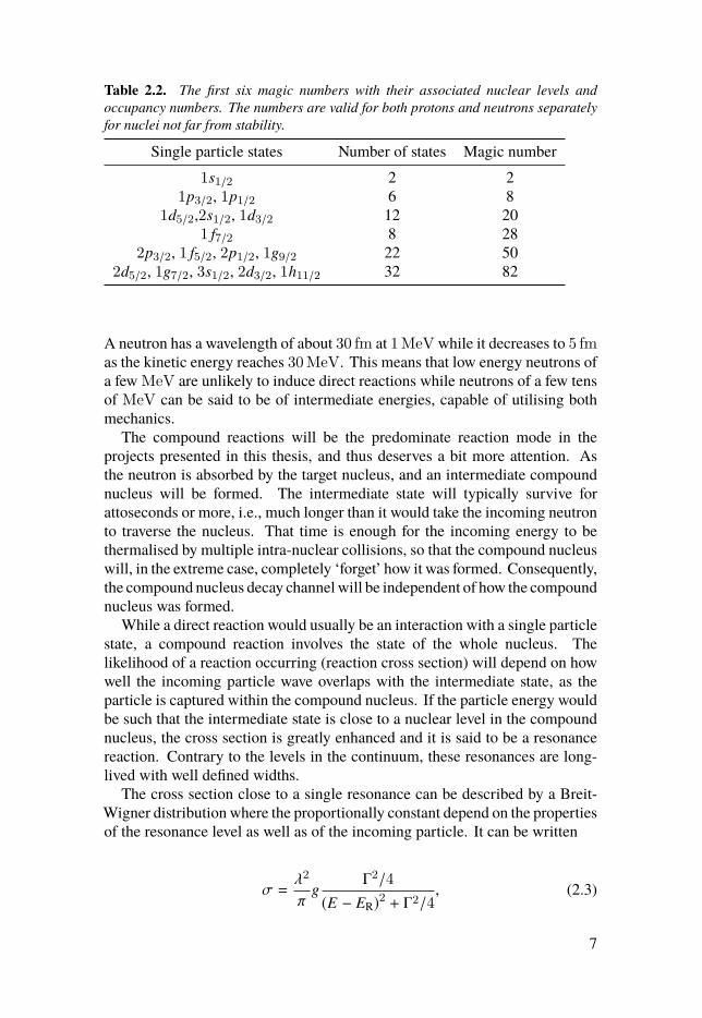
Table 2.2. The first six magic numbers with their associated nuclear levels andoccupancy numbers. The numbers are valid for both protons and neutrons separatelyfor nuclei not far from stability.

Single particle states Number of states Magic number1s1/2 2 2

1p3/2, 1p1/2 6 81d5/2,2s1/2, 1d3/2 12 20

1 f7/2 8 282p3/2, 1 f5/2, 2p1/2, 1g9/2 22 50

2d5/2, 1g7/2, 3s1/2, 2d3/2, 1h11/2 32 82

A neutron has a wavelength of about 30 fm at 1MeV while it decreases to 5 fmas the kinetic energy reaches 30MeV. This means that low energy neutrons ofa few MeV are unlikely to induce direct reactions while neutrons of a few tensof MeV can be said to be of intermediate energies, capable of utilising bothmechanics.

The compound reactions will be the predominate reaction mode in theprojects presented in this thesis, and thus deserves a bit more attention. Asthe neutron is absorbed by the target nucleus, and an intermediate compoundnucleus will be formed. The intermediate state will typically survive forattoseconds or more, i.e., much longer than it would take the incoming neutronto traverse the nucleus. That time is enough for the incoming energy to bethermalised by multiple intra-nuclear collisions, so that the compound nucleuswill, in the extreme case, completely ‘forget’ how it was formed. Consequently,the compound nucleus decay channel will be independent of how the compoundnucleus was formed.

While a direct reaction would usually be an interaction with a single particlestate, a compound reaction involves the state of the whole nucleus. Thelikelihood of a reaction occurring (reaction cross section) will depend on howwell the incoming particle wave overlaps with the intermediate state, as theparticle is captured within the compound nucleus. If the particle energy wouldbe such that the intermediate state is close to a nuclear level in the compoundnucleus, the cross section is greatly enhanced and it is said to be a resonancereaction. Contrary to the levels in the continuum, these resonances are long-lived with well defined widths.

The cross section close to a single resonance can be described by a Breit-Wigner distribution where the proportionally constant depend on the propertiesof the resonance level as well as of the incoming particle. It can be written

σ =λ2

πg

Γ2/4(E − ER)2 + Γ2/4

, (2.3)

7

where λ is the particle wavelength, Γ the resonance width, E the particleenergy, and ER the resonance energy. The statistical factor g describe howthe incoming particle spin sp, and the target nucleus spin sn, can couple withthe orbital angular momentum �, to match the total angular momenta I of theresonance:

g =2I + 1

(2sp + 1)(2sn + 1). (2.4)

In addition of affecting the cross section, the resonance state will also affectangular distributions of emitted particles. Resonance reactions are of particularimportance in the measurement described in chapter 6.

2.4 FissionMany heavy nuclei can undergo spontaneous fission, but the naturally abundantones will do so only at low rates. Fission of a nucleus can also be induced,if an incoming particle is absorbed. For charged particles this means that theCoulomb repulsion must be overcome in order to reach the nucleus, whileγ- and neutron-induced fission are not affected by this. The discussion willmostly be restricted to neutron-induced fission, which is the most relevant forthis thesis.

Regardless of how the fission process was initiated, it will typically lead toa heavy nucleus being split into two highly excited Fission Fragments (FFs)of about half the mass of the fissioning nucleus and an energy release of about200MeV. The energy comes from the fact that the mass of the final state isless than the original nucleus, since the daughter nuclei are more tightly bound.

Occasionally, other light particles can be emitted in the moment of scission.These are predominately α-particles and are referred to as ternary particlescoming from a ternary fission. In binary fission, the two heavy FFs repel eachother and leave the fission site collinearly. If a ternary particle is present thecollinearity is broken, but due to the mass differences the ternary particle leavein almost a straight angle to the FFs’ trajectories, repulsed by the Coulombforce. Since ternary fission is much less likely than binary, the discussion isrestricted to the binary case although many things are applicable to ternaryfission as well.

The energy that was not transformed into kinetic energy is stored as excit-ation energy in the newly formed nuclei. Both FFs will have, on average, asimilar ratio of neutrons to protons as the mother nucleus. However, sincea FF is much lighter than the mother nucleus, it has a neutron excess, i.e.,more neutrons than any stable isotopes of the specific element. Neutrons aretherefore easily emitted if enough excitation energy is available to pay for theneutron separation energy. In general, as many neutrons as possible are emittedby the excited nucleus, until the excitation energy is so low that deexcitation is

8

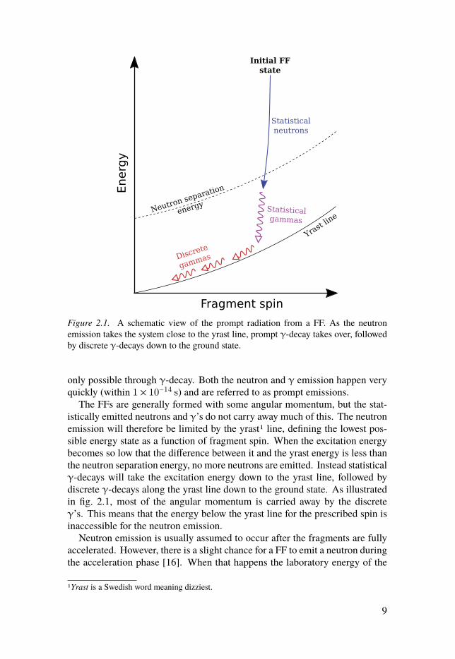
Figure 2.1. A schematic view of the prompt radiation from a FF. As the neutronemission takes the system close to the yrast line, prompt γ-decay takes over, followedby discrete γ-decays down to the ground state.

only possible through γ-decay. Both the neutron and γ emission happen veryquickly (within 1 × 10−14 s) and are referred to as prompt emissions.

The FFs are generally formed with some angular momentum, but the stat-istically emitted neutrons and γ’s do not carry away much of this. The neutronemission will therefore be limited by the yrast1 line, defining the lowest pos-sible energy state as a function of fragment spin. When the excitation energybecomes so low that the difference between it and the yrast energy is less thanthe neutron separation energy, no more neutrons are emitted. Instead statisticalγ-decays will take the excitation energy down to the yrast line, followed bydiscrete γ-decays along the yrast line down to the ground state. As illustratedin fig. 2.1, most of the angular momentum is carried away by the discreteγ’s. This means that the energy below the yrast line for the prescribed spin isinaccessible for the neutron emission.

Neutron emission is usually assumed to occur after the fragments are fullyaccelerated. However, there is a slight chance for a FF to emit a neutron duringthe acceleration phase [16]. When that happens the laboratory energy of the

1Yrast is a Swedish word meaning dizziest.

9

3−

10

2−10

1−10

A

80 90 100 110 120 130 140 150 160 170

Excitation e

nerg

y / M

eV

0

10

20

30

40

50

60

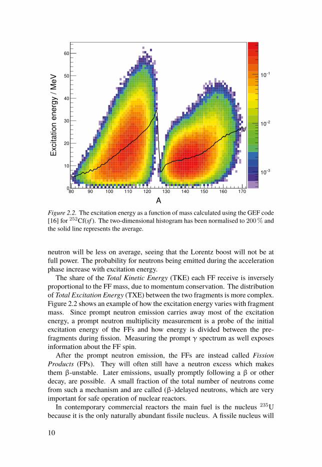
Figure 2.2. The excitation energy as a function of mass calculated using the GEF code[16] for 252Cf(sf ). The two-dimensional histogram has been normalised to 200% andthe solid line represents the average.

neutron will be less on average, seeing that the Lorentz boost will not be atfull power. The probability for neutrons being emitted during the accelerationphase increase with excitation energy.

The share of the Total Kinetic Energy (TKE) each FF receive is inverselyproportional to the FF mass, due to momentum conservation. The distributionof Total Excitation Energy (TXE) between the two fragments is more complex.Figure 2.2 shows an example of how the excitation energy varies with fragmentmass. Since prompt neutron emission carries away most of the excitationenergy, a prompt neutron multiplicity measurement is a probe of the initialexcitation energy of the FFs and how energy is divided between the pre-fragments during fission. Measuring the prompt γ spectrum as well exposesinformation about the FF spin.

After the prompt neutron emission, the FFs are instead called FissionProducts (FPs). They will often still have a neutron excess which makesthem β-unstable. Later emissions, usually promptly following a β or otherdecay, are possible. A small fraction of the total number of neutrons comefrom such a mechanism and are called (β-)delayed neutrons, which are veryimportant for safe operation of nuclear reactors.

In contemporary commercial reactors the main fuel is the nucleus 235Ubecause it is the only naturally abundant fissile nucleus. A fissile nucleus will

10

gain enough energy, by absorbing even a thermal neutron, to overcome thefission barrier. The fission barrier is a term used to describe how the systemmust first go up in potential energy as the short-ranged strong force weakenswhen the nucleus starts separating into two parts. While quantum mechanicalsystems can tunnel through barriers, it is much more likely for a system topass a barrier if a large excitation energy is present. When a nucleus absorbs aneutron, it gains the neutron separation energy as excitation energy in additionto the kinetic energy contribution, as the neutron becomes bound.

How much energy is gained will vary. 235U is a nucleus with an even numberof protons, but odd number of neutrons. Pairing the absorbed neutron with thelast valence neutron is favoured, since the spins can be opposed and therebyminimises the angular momentum. In effect, the new nucleon is more tightlybound, leaving more energy as excitation energy.

In the 235U case, 6.5MeV is gained, which is enough to overcome thefission barrier of 236U. Contrary, for the non-fissile nucleus 238U, the absorbedneutron cannot pair up and consequently the resulting binding energy is lower.In turn, that leads to a lower excitation energy of 4.8MeV in the compoundsystem 239U which is below the barrier height. Not until the incoming neutroncarries about 2MeV can the 239U nucleus pass the fission barrier with ease.Such nuclei, that need the incoming neutron to carry enough energy to be ableto get above the fission barrier are called fissionable. In the case with 239U itcan form the fissile nucleus 239Pu through two subsequent β-decays, which iswhy 238U is also called fertile.

The presence of a fission barrier can be explained by the Liquid Drop Model,but many of the detailed properties of fission requires a more advanced model.The LDM in its simplest form only account for the nucleus’ volume, surface,and Coulomb repulsion (but usually also includes the asymmetry and pairingterms). Therefore, it can predict many average properties and general trends,but misses out on specific interactions between the single-particle states. Onthe other hand, just summing all single-particle energies, which obviouslytakes shell effects into account, have not had much success reproducing allmacroscopic quantities. Strutinsky realised how the two approaches couldbe combined by taking the energy calculated using the LDM and adding acorrection term based on the average shell effects [17]. This can be performedfor different nuclear shapes and deformations, thus creating an energy potentiallandscape describing the fission barrier.

Already the separation distance of the two mass centres can explain severalfeatures of the fission barrier. As the nucleus elongates, shell structure playsan important role in determining the shape of the barrier. The energeticallyfavoured states will shift as the distance increases. When an occupied statecrosses another state with the same spin and parity, the most energeticallyfavoured state will become the occupied one. This phenomena creates a localwell on top of the fission barrier and appears as soon as the shell effects aretaken into account, even in the average form devised by Strutinsky [17].

11

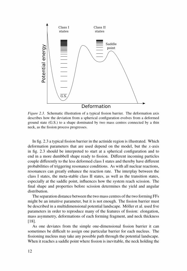
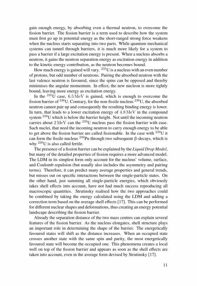
Figure 2.3. Schematic illustration of a typical fission barrier. The deformation axisdescribes how the deviation from a spherical configuration evolves from a deformedground state (G.S.) to a shape dominated by two mass centres connected by a thinneck, as the fission process progresses.

In fig. 2.3 a typical fission barrier in the actinide region is illustrated. Whichdeformation parameters that are used depend on the model, but the x-axisin fig. 2.3 should be interpreted to start at a spherical configuration and toend in a more dumbbell shape ready to fission. Different incoming particlescouple differently to the less deformed class I states and thereby have differentprobabilities of triggering resonance conditions. As with all nuclear reactions,resonances can greatly enhance the reaction rate. The interplay between theclass I states, the meta-stable class II states, as well as the transition states,especially at the saddle point, influences how the system reach scission. Thefinal shape and properties before scission determines the yield and angulardistribution.

The separation distance between the two mass centres of the two forming FFsmight be an intuitive parameter, but it is not enough. The fission barrier mustbe described in a multidimensional potential landscape. Möller et al. used fiveparameters in order to reproduce many of the features of fission: elongation,mass asymmetry, deformations of each forming fragment, and neck thickness[18].

As one deviates from the simple one-dimensional fission barrier it cansometimes be difficult to assign one particular barrier for each nucleus. Thefissioning nucleus may take any possible path through the potential landscape.When it reaches a saddle point where fission is inevitable, the neck holding the

12

nucleus together will get thinner and longer until it raptures and two separateFFs are formed. Every path is possible, but not equally probable due to itsunique way of traversing the multi-dimensional fission barrier. Fission of anucleus like 236U is dominated by asymmetric modes [19] while symmetricpre-fission shapes are much less likely. A simple explanation for this is thatthe heavier of the forming FFs can lower the system’s energy by adaptinga near spherical shape close to the doubly magic 132

50 Sn configuration. Theasymmetric pre-fission shape then naturally leads to the an asymmetric massdistribution as the FFs are formed.

It is observed experimentally, that while the light mass peak move with thecompound nucleus mass, the heavy mass peak stays more or less the sameover a large range of fissioning systems in the actinide region. This is in goodagreement with the closure of the Z = 50 and the N = 82 shells. The lightfragment in this mass region does not have any shell closures in range andis therefore less restricted to any certain mass numbers. As the energy of theincoming neutron is increased, the higher potential barrier of symmetric fissionbecomes less important, thus making the symmetric mode more competitive.

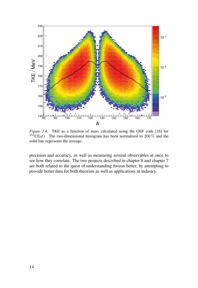
The TKE as a function of mass increase as the the two fragments get similarmasses, since the Coulomb repulsion is proportional to the product Z1 · Z2.In the case of 252Cf(sf ) the Q-value also peaks close to symmetry leaving amaximum amount of energy available. However, close to symmetry the TKEexhibits a local minimum (fig. 2.4). This is a sign of a different fission modein this mass region: a Super Long (SL) mode in the terminology of Brosaet al. [19], where the two mass centres are formed at a greater distance whichdecreased Coulomb potential energy as a consequence.

In an attempt to find out how fission proceeds Randrup and Möller allowedthe system to take random walks [20] on their calculated five-dimensional po-tential landscapes [18]. The walk was not entirely random since the probabilityof each step was weighted by the potential difference in a similar fashion as inthe famous work of Metropolis et al. [21]. That is, the system is allowed, butdiscouraged, to step up in potential energy. Observing where in the potentiallandscape the walks end up, i.e., how scission is reached, gives a picture of theevolution of the fission process.

The angular distribution of the FFs, with respect to the incoming neutron,is an important experimental observable since it contains information aboutthe states and modes [19] during the fission process. As new transition statesbecome energetically available the Fission Fragment Angular Distribution(FFAD) is influenced by the quantum numbers of those states making it ahighly energy dependant observable. Especially when new chances of fissionopen up with increased neutron energies [22], the deviation from isotropicemission (anisotropy) of FFs can suddenly change due to the completely newstates that become available.

Fission is a complicated many-body system that we still lack detailed un-derstanding of. It is therefore still interesting to measure FP yields to greater

13

3−

10

2−10

1−10

A

80 90 100 110 120 130 140 150 160 170

TK

E / M

eV

140

150

160

170

180

190

200

210

220

230

Figure 2.4. TKE as a function of mass calculated using the GEF code [16] for252Cf(sf ). The two-dimensional histogram has been normalised to 200% and thesolid line represents the average.

precision and accuracy, as well as measuring several observables at once tosee how they correlate. The two projects described in chapter 8 and chapter 7are both related to the quest of understanding fission better, by attempting toprovide better data for both theorists as well as applications in industry.

14

3. Particle detectors

Your ”discovered boson“ which wasdetected in the LHC, is simply oneXenon atom of the 1 trillion 167billion 20 million Xenon atoms whichthere are in the LHC!

— Gabor Fekete

The choice of detector depends on the situation and will be affected by, e.g.,particle species, solid angle coverage, background situation, and of coursewhat information the experimentalist is after. In all of the experiments coveredby this thesis, the detected particles are either heavy nuclei, i.e. FPs, or lightcharged particles (p, d, t, 3He, or α-particles). In none of them are neutronsever directly detected. In particular, the different stopping ranges of theseparticles, give rise to different preferences and challenges when one tries todecide on a suitable detector system.

The most straight forward way of detecting a fission event is by detectingthe FPs. As they are heavy ions, they give rise to high amplitude signalsin many gas detectors and near 100% detection efficiency. However, for thesame reason they also suffer from short stopping ranges even in low densitymaterials. In solid state detectors the charge density due to the stopping of theions give rise to plasma effects that must be compensated for. In thick targetsmany FPs will not be able to reach the outside of the target. Thin targets can bemade through different kinds of deposition techniques [23, 24]. The kinematicscan also be of help, especially if both fragments are detected, since they willtypically travel in almost opposite directions in both the Centre-of-Momentum(CoM) and the laboratory frame of reference. However, due to the incomingmomentum of the neutron and the prompt neutron emission, the fragmentswill generally have an angle different from 180° between them. This leadsto a requirement for a larger solid angle coverage, which often is easier usinggaseous detectors.

Contrary to the FPs, light particles like protons can be detected in solid statedetector, e.g. silicon detectors, with high resolution. The high penetrationof these particles can make them more difficult to detect in gas detectors, butalready α-particles have a significantly shorter stopping range than protons.

In the following sections I will describe the different detectors used in thisthesis, and try to outline how they work as well as their most basic properties.

15

3.1 Frisch-gridded ionisation chambersA non-gridded gas detector can be used to measure the energy a particledeposits in the detection gas. It is simply a volume of gas with an appliedelectric field across it. When an ionising particle is stopped in the chambergas, the energy it deposits in the stopping material enables the atomic ormolecular electrons to break free from their orbits, effectively creating pairs ofpositive ions and free electrons. The number of pairs are proportional to theamount of energy lost by the particle. As we will see later on, the positive ionsare of less interest since their contribution to the obtained electronic signalscan be completely neglected.

However, in such a setup, the signals induced on the electrodes will not bestraight forward to analyse. The distance to the electrode, at which the electronsare created, influences the amount of charge that is induced on the electrode.There is a remedy for this though. By introducing a conducting grid betweenthe cathode and anode at an intermediate bias it is possible to get an anodesignal proportional the energy and also deduce the angle of the particle, giventhat it originates from the cathode, i.e. the target or sample should be placedon or be part of the cathode. This kind of setup goes under the name Frisch-Gridded Ionisation Chamber or just Gridded Ionisation Chamber (GIC). Howit works will be described in the following section.

3.1.1 Obtaining angular informationIn order to later follow the discussion of the signal analysis more easily, it iswell worth spending some time seeing how these signals are generated in somedetail. Some handy notation, that will be used subsequently, is collected intable 3.1. Most of the notation is also depicted in fig. 3.1 or fig. 3.2. To beginwith, we will assume that the conducting grid completely shields the anodefrom the cathode and vice versa. We will also assume that it is 100% transparentto electrons. None of these assumptions are completely true, but correctionsfor deviations from this ideal model can be made later. The electrode voltagesshould be chosen with the transparency in mind. For mesh grids, a study hasbeen made by Bevilacqua et al. in Ref. [25].

When an electric charge q, drifts towards an electrode it will induce a currenton the electrode. The integrated charge Q can be expressed as

Q = q(ϕ(x f ) − ϕ(xi)

), (3.1)

where Q is a function of the weighting potential ϕ(x), according to theShockley-Ramo theorem [26]. The weighting potential is evaluated at thefinal, respectively initial, position of the moving charge q. The weightingpotential is similar to the electric potential in absence of the moving charge,but it is a unitless quantity, with unit value on the electrode of interest andzero on all other conductors. That is, it is independent of the actual values

16

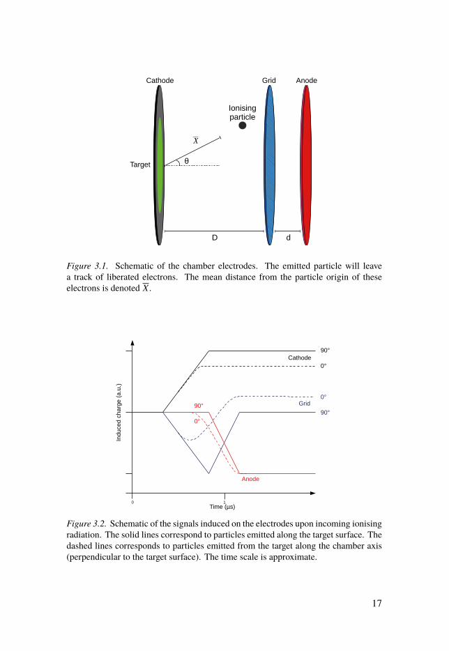
Figure 3.1. Schematic of the chamber electrodes. The emitted particle will leavea track of liberated electrons. The mean distance from the particle origin of theseelectrons is denoted X .

Figure 3.2. Schematic of the signals induced on the electrodes upon incoming ionisingradiation. The solid lines correspond to particles emitted along the target surface. Thedashed lines corresponds to particles emitted from the target along the chamber axis(perpendicular to the target surface). The time scale is approximate.

17

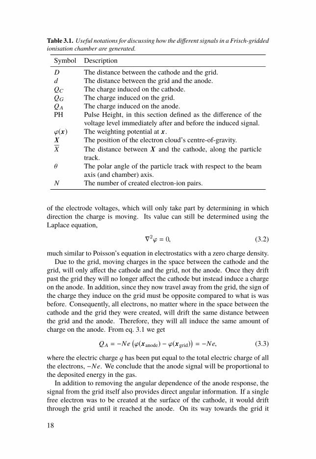
Table 3.1. Useful notations for discussing how the different signals in a Frisch-griddedionisation chamber are generated.

Symbol DescriptionD The distance between the cathode and the grid.d The distance between the grid and the anode.QC The charge induced on the cathode.QG The charge induced on the grid.QA The charge induced on the anode.PH Pulse Height, in this section defined as the difference of the

voltage level immediately after and before the induced signal.ϕ(x) The weighting potential at x.X The position of the electron cloud’s centre-of-gravity.X The distance between X and the cathode, along the particle

track.θ The polar angle of the particle track with respect to the beam

axis (and chamber) axis.N The number of created electron-ion pairs.

of the electrode voltages, which will only take part by determining in whichdirection the charge is moving. Its value can still be determined using theLaplace equation,

∇2ϕ = 0, (3.2)

much similar to Poisson’s equation in electrostatics with a zero charge density.Due to the grid, moving charges in the space between the cathode and the

grid, will only affect the cathode and the grid, not the anode. Once they driftpast the grid they will no longer affect the cathode but instead induce a chargeon the anode. In addition, since they now travel away from the grid, the sign ofthe charge they induce on the grid must be opposite compared to what is wasbefore. Consequently, all electrons, no matter where in the space between thecathode and the grid they were created, will drift the same distance betweenthe grid and the anode. Therefore, they will all induce the same amount ofcharge on the anode. From eq. 3.1 we get

QA = −Ne(ϕ(xanode) − ϕ(xgrid)

)= −Ne, (3.3)

where the electric charge q has been put equal to the total electric charge of allthe electrons, −Ne. We conclude that the anode signal will be proportional tothe deposited energy in the gas.

In addition to removing the angular dependence of the anode response, thesignal from the grid itself also provides direct angular information. If a singlefree electron was to be created at the surface of the cathode, it would driftthrough the grid until it reached the anode. On its way towards the grid it

18

would induce a negative charge and after passing the grid it would induceexactly the same charge but with opposite sign. The final Pulse Height (PH) ofthe grid signal would be zero. If the electron instead was created further awayfrom the cathode, the charge induced on the grid while travelling towards it,would be less since the distance travelled would be less. The final PH of thegrid signal would in this case be positive. This effect can be exploited in orderto determine the angle of the incoming particle. We will see how this can bedone, by deriving an expression for the PH of the induced charge on the grid,QG .

The weighting potential at a position x between the two electrodes can beapproximated to a linear function by assuming that the electrodes are infiniteparallel plates and integrating eq. 3.2 twice. That is, if x is the distance fromthe cathode and D, the cathode-grid distance, ϕ can be written

ϕ = 1 − xD. (3.4)

Since the detector response is due to many moving charges rather than asingle electron, they are treated as if they were a single charge −Ne, created atthe centre-of-gravity X of the electron cloud. To find the induced charge on thecathode, the Shockley-Ramo theorem (eq. 3.1) is applied using the potentialfrom Eq. 3.4,

QC = −Ne(ϕgrid − ϕ(X)) = Ne

(1 − X

Dcos θ

)(3.5)

where X has been projected onto the chamber axis. The induced charge on thegrid is found by noting that the total induced charge on the electrodes shouldbe zero, i.e. QC +QG +QA = 0. The charge induced on the grid is therefore

QG = −QC − QA = NeXD

cos θ. (3.6)

We have now derived an expression that shows how the grid signal will beproportional to the cosine of the particle angle with respect to the chamber axis.It is not necessary to actually measure the bi-polar grid signal, since one couldjust use the difference of the anode and cathode. However, the cathode andanode signals would go through different electronic amplification chains, andthe difference would be more sensitive to fluctuations in the electronics. Also,in setups with a thin fission target both FPs will affect the cathode, makingit difficult to disentangle the two contributions. With modern equipmentincluding digitisers, it is straight forward to measure the grid signal and deducethe PH directly [27].

Until now, the slow positive ions have been neglected. The positive ionstravel towards the cathode and therefore the inducted charge, Qion

C,G,A, due to

19

the heavy ions becomes:

QionC = −Ne

(1 − X

Dcos θ

), Qion

G = −QionC and Qion

A = 0. (3.7)

The ions are about four orders of magnitude more massive than the electrons, sothey have barely moved during the time the electrons were collected. Therefore,the charge induced by the positive ions during the time it takes to collect theelectrons, on either the grid or the cathode, is negligible. The induction due tothe heavy ions is usually not observed at all, due to the much longer time scaleit happens on.

The above derivation was based on a perfect grid. In reality the grid willallow part of the electric field to leak through and therefore the anode is affectedby the electrons even before they pass the grid. The effect is in the order of afew percent and can be corrected for. A parametrisation of the so called gridinefficiency has been made by Göök et al., derived for different types of grids[28].

3.1.2 Loss of charge and choice of gasSince the last region the electrons will pass through is the one between thegrid and the anode (the region where the induced charge will increase the gridPH), any loss of electrons will manifest itself as a more negative grid signal.In order for the electrons to pass through the grid without losses the fieldstrength between the grid and the anode must be several times higher than thefield strength between the cathode and the grid. This has been investigated byBevilacqua et al. [25] for mesh grids, which behave differently to parallel-wiregrids.

The detection gas is of importance because it will, among other things,determine the stopping power of the incoming radiation and the migrationspeed of the electrons. A high migration speed will reduce timing uncertaintiesas well as the chance of absorption of the electron. It is also important to havea constant migration speed in case the electrode voltages or the gas pressurewould fluctuate a little bit. This is achieved by observing where the migrationspeed as a function of the reduced voltage hits a plateau (often the drift velocitysaturates at high field strengths). At which voltages the plateau is found dependson the choice of detection gas or gas mixture.

The choice of gas will also affect the rate of negative ion formation aselectrons are absorbed by the gas atoms or molecules. Especially the highlyelectron negative oxygen can play a big role since a small oxygen contaminationcan completely ruin the detector performance. An additive to the main gas, e.g.methane added to argon, can be advantageous since the added minority gascan de-excite meta-stable gas particles of the majority gas by collisions. Thisimproves the energy resolution. As ionisation chambers typically are operated

20

below the proportional region no Townsend avalanches occurs and quenchingis not needed. Suitable gas, pressure and electrode voltages are imperative forstable operation.

3.2 Parallel plate avalanche countersThe Parallel Plate Avalanche Counters (PPACs) are gas-filled detectors whichconsist of two parallel foils (often aluminised Mylar, polyethylene terephthalate,[C10O4H8]n). They are commonly used to detect heavy ions [29–31]. Theyare typically operated at a gas pressure of a few mbar. A thin layer (muchthinner than the foil thickness) of aluminium deposited on a Mylar foil, allowsfor a high voltage to be applied over the gap between the foils. Upon anionising event, this voltage will affect the electrons that are released. As theydrift towards the anode, their movement will induce a voltage which will bethe signal one measures. The signal is amplified by the gas multiplicationprocess due to the high field strength. Although the PPACs are operated inproportional mode, where the induced charge on the anode is proportional tothe initial number of ionisations, the energy resolution is typically not betterthan 20% (ΔEE ) [29].

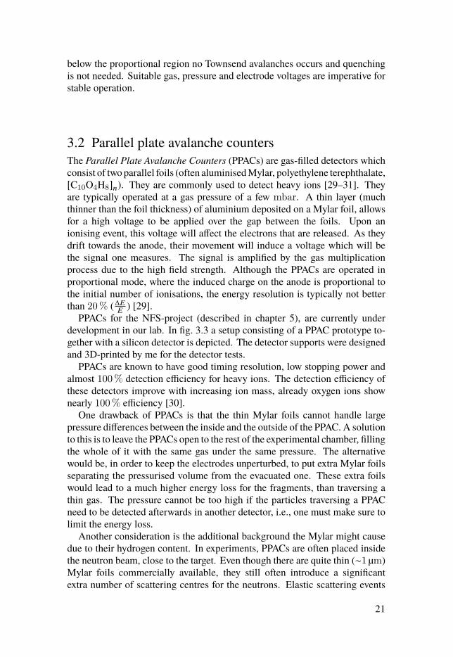
PPACs for the NFS-project (described in chapter 5), are currently underdevelopment in our lab. In fig. 3.3 a setup consisting of a PPAC prototype to-gether with a silicon detector is depicted. The detector supports were designedand 3D-printed by me for the detector tests.

PPACs are known to have good timing resolution, low stopping power andalmost 100% detection efficiency for heavy ions. The detection efficiency ofthese detectors improve with increasing ion mass, already oxygen ions shownearly 100% efficiency [30].

One drawback of PPACs is that the thin Mylar foils cannot handle largepressure differences between the inside and the outside of the PPAC. A solutionto this is to leave the PPACs open to the rest of the experimental chamber, fillingthe whole of it with the same gas under the same pressure. The alternativewould be, in order to keep the electrodes unperturbed, to put extra Mylar foilsseparating the pressurised volume from the evacuated one. These extra foilswould lead to a much higher energy loss for the fragments, than traversing athin gas. The pressure cannot be too high if the particles traversing a PPACneed to be detected afterwards in another detector, i.e., one must make sure tolimit the energy loss.

Another consideration is the additional background the Mylar might causedue to their hydrogen content. In experiments, PPACs are often placed insidethe neutron beam, close to the target. Even though there are quite thin (∼1 μm)Mylar foils commercially available, they still often introduce a significantextra number of scattering centres for the neutrons. Elastic scattering events

21

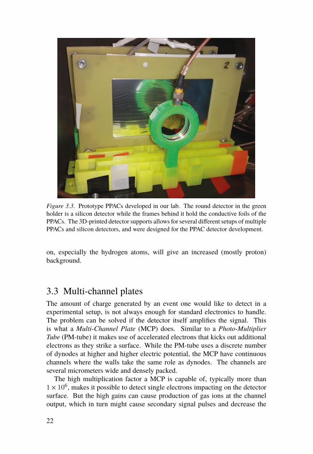
Figure 3.3. Prototype PPACs developed in our lab. The round detector in the greenholder is a silicon detector while the frames behind it hold the conductive foils of thePPACs. The 3D-printed detector supports allows for several different setups of multiplePPACs and silicon detectors, and were designed for the PPAC detector development.

on, especially the hydrogen atoms, will give an increased (mostly proton)background.

3.3 Multi-channel platesThe amount of charge generated by an event one would like to detect in aexperimental setup, is not always enough for standard electronics to handle.The problem can be solved if the detector itself amplifies the signal. Thisis what a Multi-Channel Plate (MCP) does. Similar to a Photo-MultiplierTube (PM-tube) it makes use of accelerated electrons that kicks out additionalelectrons as they strike a surface. While the PM-tube uses a discrete numberof dynodes at higher and higher electric potential, the MCP have continuouschannels where the walls take the same role as dynodes. The channels areseveral micrometers wide and densely packed.

The high multiplication factor a MCP is capable of, typically more than1 × 106, makes it possible to detect single electrons impacting on the detectorsurface. But the high gains can cause production of gas ions at the channeloutput, which in turn might cause secondary signal pulses and decrease the

22

detector life time [32]. This problem is reduced by angling the channels, andfurther reduced by combining two plates in a so called chevron, i.e. v-shaped,configuration. Three plates are sometimes combined, in a similar fashion, intoa so called Z-stack. Every incoming particle on the MCP will decrease its lifetime, why it is important to shield it from unnecessary exposure.

As the amplification is usually limited by space charges, it is not a suitabledetector for energy measurements since the output signal will not be propor-tional to the incoming energy. After a saturation voltage over the MCP plate(s)has been reached further increasing the voltage will worsen the resolution[33]. It is however suitable for measuring time, since it is capable of a timingresolution in the order of hundreds to tens of ps [32, 33].

3.4 Silicon detectorsSemiconductor detectors, and especially silicon detectors, are very commondetectors for a number of applications. For both experiments discussed inchapters 5 and 7 the silicon detectors are a main ingredient to the experimentalsetup. In both cases the detectors are used to detect both light and heavycharged particles. The detectors discussed here are of the type Silicon SurfaceBarrier (SSB) detectors, where either the n-type material at the diode junctioninterface is replaced by a metal, e.g., aluminium evaporated onto the siliconp-type crystal surface, or where a combination of etching and metal depositionis performed on an n-type crystal [34]. These detectors exhibit thin dead layers,essential for measuring particles with short stopping ranges.

One can divide the design of silicon detectors into two types: transmissiontype detectors, where particles with sufficient energy are supposed to penetratethe complete thickness of the silicon, and non-transmission type detectors,where the particle is supposed to be stopped within the thickness of the detector.The first type is always operated fully depleted, but that is not necessary forthe latter mentioned type since the sensitive region do not need to extend overthe penetration depth of the measured radiation.

A typical silicon detector will give about one electron per 3.6 eV depositedenergy. Although the band gap is 1.1 eV not all deposited energy producesnew free charges. The resolution for medium heavy particles is typically about100 keV. Detecting light particles in well controlled environments using smalldetectors can decrease this value down to about 10 keV [34, p. 403].

For reasonably light particles, the stopping power and therefore also the rateof energy depositing in the detector material decreases with energy. It is alsohighly dependent on the charge of the particle. Both these dependencies canbe utilised to determine the particle species in a, so called, telescope setup(see fig. 3.4). This method is commonly referred to as the ΔE-E method, andas the name suggests it is based on letting the particle first go through a (orseveral) thin transmission type detector(s) where it only deposits part of its

23

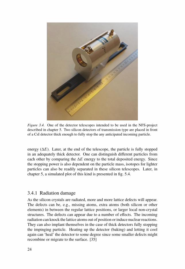
Figure 3.4. One of the detector telescopes intended to be used in the NFS-projectdescribed in chapter 5. Two silicon detectors of transmission type are placed in frontof a CsI detector thick enough to fully stop the any anticipated incoming particle.

energy (ΔE). Later, at the end of the telescope, the particle is fully stoppedin an adequately thick detector. One can distinguish different particles fromeach other by comparing the ΔE energy to the total deposited energy. Sincethe stopping power is also dependent on the particle mass, isotopes for lighterparticles can also be readily separated in these silicon telescopes. Later, inchapter 5, a simulated plot of this kind is presented in fig. 5.4.

3.4.1 Radiation damageAs the silicon crystals are radiated, more and more lattice defects will appear.The defects can be, e.g., missing atoms, extra atoms (both silicon or otherelements) in between the regular lattice positions, or larger local non-crystalstructures. The defects can appear due to a number of effects. The incomingradiation can knock the lattice atoms out of position or induce nuclear reactions.They can also implant themselves in the case of thick detectors fully stoppingthe impinging particle. Heating up the detector (baking) and letting it coolagain can ‘heal’ the detector to some degree since some smaller defects mightrecombine or migrate to the surface. [35]

24

A defect will often act as a recombination centre, thereby decreasing theoutput pulse. It might also act as a trapping centre where charges can besufficiently delayed in order for them not to register together with the mainpulse, effectively lowering the detected pulse height. The radiation damage insilicon detectors can be monitored by observing the leakage current. Duringlong radiations the leakage current steadily increases as the crystal lattice in thedetector gets more distorted. Especially defects that contribute energy statesinside the band gap can increase the leakage current significantly. [35]

3.4.2 Detecting heavy ions in silicon detectorsComplications arise as the detected particles get heavier. For a given energy,heavier particles are slower, which give them more opportunities to pick upstray electrons from their surroundings. When a heavy ion travels througha material an equilibrium will be found where the ion continuously picks upand loses electrons at the same rate. The mean equilibrium charge (effectivecharge) can be parametrised to be a function mainly dependent on the atomiccharge of both the ion and the surrounding atoms, as well as on the velocity ofthe ion [36, p. 216, 37]. Consequently, the stopping power of different FPs arecomparable, the effective charge smoothing out the charge dependence, andcontrary to light ions the stopping power is often the highest at the beginningof the particle trace. The short stopping range of low energetic (no more than∼100MeV) heavy ions would anyway inhibit the use of a telescope setup forisotope identification, unless the ΔE detector is extremely thin.

The next complication for detecting heavy ions in silicon detectors arisesfrom the high stopping power and the accompanying short stopping range.The cloud of free charges, i.e. a plasma, released due to the stopping process,will be concentrated in a fairly small volume. The more plasma, the biggerthe effects of shielding. The electrons will feel much less of the detector biaswhen surrounded by a dense plasma, i.e., all the other electrons and positiveholes. For the experimentalist the plasma will affect both time and energymeasurements.

The charge collection time will be longer because of the reduced electricfield visible to the charges. The Plasma Delay Time (PDT) is in the order of2 ns for FPs. For a flight time measurement this translates into a relative errorof several percents if a the flight path is in the order of a meter.

The extra delay gives all the freed charges extra time to recombine beforethey are separated by the detector bias. For every electron-hole pair thatrecombines a smaller output signal will be seen. Also, a small fraction of theheavy ions stopping will be due to collisions with the silicon nuclei, and energyloss not due to collisions with electrons will not create electron-hole pairs tobegin with. In addition, even thin dead layers can cause sizeable energy losses.

25

All these three phenomena contribute to what is called Pulse Height Defect(PHD).

All together these effects can cause a PHD well exceeding 10MeV. A highdetector bias can suppress the PHD to a minimum but it will still be sizeable. Acommon way of addressing this is to make a mass dependent energy calibration[38], with the obvious downside that one must know the mass of the ion beforeone can get an accurate energy reading of it. This kind of energy calibrationand its implementation in the analysis of the VERDI data is further discussedin section 7.7.2.

26

4. Neutron facilities

Given enough startup capital and anadequate research facility, I could beBatman.

— Sheldon Cooper

All the experiments discussed in this thesis require a neutron source at somepoint in their project lifetimes. Creating strong neutron sources is not trivialsince the primary beam will have to be charged particles that in turn createsa secondary neutron beam. What facility is suitable for an experiment willdepend on the desired neutron energies, the cross section of the studied reactionwhich might require high neutron fluxes, time-of-flight (ToF) possibilities,background conditions, additional available research infrastructure etc.

The experiments related to the projects presented in chapters 5, 6 and 8 resideat three different facilities (NFS, GELINA and IGISOL, respectively) brieflyintroduced below. The VERDI spectrometer presented in chapter 7 is still ina development phase, but might be used at several different neutron facilitiesupon completion, depending on what beams are available and desirable.

4.1 NFSThe Neutron For Science (NFS) facility [39, 40] at GANIL in Caen, France,is part of the first phase of the SPIRAL2 project [41]. The facility is not yetoperational, but the accelerator is installed and under commissioning. The planis to have two main options for neutron production available. A continuousneutron spectrum, through the deuteron break-up reaction in a thick (8mm)beryllium target, and a Quasi Mono-energetic Neutron (QMN) spectra throughthe 7Li(p,n) reaction on a thin target. A high flux beam up to about themaximum deuteron energy of 40MeV is expected from the continuous option.Using the QMN beam the peak energy can be chosen up to the maximumproton energy of 33MeV.

The primary beam frequency of 88MHz will be reduced by a factor of100 to 10 000 by using a chopper. The maximum current on the converter isdesigned to be 50 μA, capable of generating an average neutron flux of about2 × 106/(MeV cm2 s) at a five metre distance when the beryllium converter isused.

The high flux enables measurements that otherwise would take very longtime and the continuous neutron energy spectrum allows experiments to cover

27

the whole energy range provided that a suitable ToF technique is used. TheToF hall offers distances from the converter target from 5 to 28m. Longerdistances enable better neutron energy resolutions but at the price of lowerneutron flux. At the moment, commissioning of the neutron beams is expectedno sooner than late 2018. The QMN option will be the first to be tested andthe full specifications will not be reached until a later date.

4.2 GELINAThe Geel Linear Accelerator (GELINA) [42, 43] is a neutron source thatresides at the European Commission’s Joint Research Centre in Geel, Bel-gium (JRC-Geel, formerly known as the Institute for Reference Materials andMeasurements, IRMM). Just like the NFS facility will, the GELINA facilityprovides a pulsed continuous neutron energy spectrum. The primary beamis a linear electron accelerator capable of delivering electrons in short pulses(1 ns FWHM), with a peak current of 120A. The electron energy can be upto 150MeV. The neutron converter is a depleted uranium target in which theelectrons are stopped emitting bremsstrahlung, which in turn causes γ-inducedfission and (γ,n) reactions. The resulting neutron spectrum is peaked around1 to 2MeV but extends up to 20MeV. The repetition rate is usually 800Hz,but the accelerator can be run at lower frequencies.

The very short primary pulses together with up to 400m long flight pathsallow high neutron energy resolutions. To increase the neutron flux in the lowenergy range a moderator is available. The unavoidable γ-radiation escapingthe neutron production target is peaked in the primary beam direction. Theneutron flight paths are at angles up to 108° relative to the primary beam’sdirection. The flight paths at the highest angles are the least affected by theγ’s.

Access to the GELINA facility for nuclear reaction or decay data meas-urements, can be granted through the EUFRAT transnational access program.The access program is operated by the JRC-Geel and also includes access toother available infrastructure.

4.3 IGISOLIGISOL stands for Ion Guide and Isotope Separator On Line and is a nuclearresearch facility at the University of Jyväskylä in Finland. Many independ-ent proton-induced fission yields of natural uranium have been measured atIGISOL over the years [44, 45], but for the work presented in this thesis wewill also take a look at a setup for neutron-induced yield measurements, thatis currently developed [46, 47].

28

The primary beam is generated by a cyclotron and has usually consisted of 25MeV or 50MeV protons, for the studies of proton-induced fission. Previouslythe current was limited to ∼10 μA but a new cyclotron with a high maximumcurrent of ∼200 μA has been installed. The new cyclotron has a maximumproton energy of 30MeV which is also the energy intended for creating thesecondary neutron beam for the neutron-induced case.

Regardless of how the fission is induced, the idea is that it will happenin a helium filled gas vessel. The helium is constantly flowing through thechamber in order to vent anything stopped in the gas. FPs that stop in thegas will follow the gas flow out of the vessel, where they are electrostaticallyaccelerated into a vacuum tube. A dipole magnet acts as the first separator,which selects an isobaric chain, i.e. ions of similar mass (mass resolving powerMΔM ∼ 500). The extracted ions will now all have the same charge, +1. Thecharge state choice is up to the experimentalist and the optimal choice could beion specific, although all the experiments have used+1 as of today. To facilitateseparation of the isobars after the mass selecting magnet, the ions can then betransported to JYFLTRAP [48]: a Penning trap with a mass resolving powerof about 1 × 105. In the trap, the ions with mass m, and charge q, matching thecyclotron frequency

νC =1

2π

qm

B, (4.1)

will be selected while the others are discarded. This is realised through amagnet producing a magnetic field B of 7T and the application of radiofrequency fields. [44]

In the end, the ions that manage to go through the whole trap are collectedon a MCP detector and thereby counted. The whole process takes less than asecond and the mass resolution is enough to separate many meta-stable statesfrom their ground state counterparts.

There are several effects in this scheme that are not fully quantified. Thestopping power as well as the energy distributions are different for differentisotopes so it is unclear how many of them stop in the helium gas. Whichcharge state they end up in is a chemical effect, i.e. element dependent, whichis difficult to model. Only the ions ending up with the correct charge statefor the measurement will have any chance of being detected. The spatialdistribution of stopped ions in the gas, might affect the extraction efficiencyfrom the gas-filled ion guide to the vacuum system, depending on how thegas flow looks like. To not be affected by all this, the yield measurements areusually made relative to a nearby isotope of the same element hopefully havingthe same net detection efficiency. The simulation work presented in chapter 8is an attempt to start quantifying the effects of stopping efficiency in the gasbetter.

29

5. Neutron standards at NFS

Prediction is very difficult, especiallyif it’s about the future.

— Niels Bohr

A measurement of three different standard cross sections (see section 2.1)relative to each other is proposed and planned for the upcoming NFS facility(see section 4.1). Two of the reactions measured are neutron-induced fissionof 235U and 238U, respectively. The third reaction is H(n,n). Even thoughthe cross section often is written H(n,n) it is usually the recoil proton that isdetected. The energy intervals in which these reactions are standards can befound in table 2.1.

At the same time, measurements of neutron-induced Light Charged Particle(LCP) production on a number of target materials are planned using the samesetup. Both the group and the experimental setup has a history of measuringlight ion production, mostly at the The Svedberg Laboratory (TSL) [49–51].Since the experimental setup already have been used and is prepared for thesekind of measurements, the focus of this chapter is mainly on the new challengesregarding the fission measurements.

This chapter will motivate why the measurements are relevant, describethe experimental setup as well as the simulations of it, and also report on thecurrent status of the project. Many of the results of the presented simulationshave previously been presented at the Nuclear Data conference 2013 [52] andas a a full-sized article in Nucl. Instrum. Meth. A [53]. The text is partlyadapted from my licentiate thesis [5].

5.1 MotivationCross section measurements of LCP are lacking in the energy region above14MeV. Taking the setup previously operated at TSL to the new NFS facilitywould allow cross section measurements up to 40MeV, supplementing existingstudies [54–57]. The cross sections will be double-differential, with respect toenergy and the emission angle of the secondary particle.

Many industrial applications exist for such cross sections. In electronics,neutron-induced single-event effects in silicon are of interest [58]. Crosssections for LCP from carbon and oxygen nuclei have applications within thefield of neutron therapy [59]. The development of new reactors, both fission

30

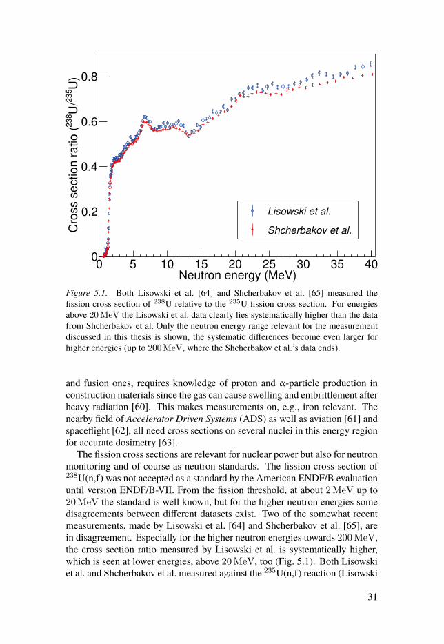
Neutron energy (MeV)0 5 10 15 20 25 30 35 40

U)

235

U/

238

Cro

ss s

ection r

atio (

0

0.2

0.4

0.6

0.8

Lisowski et al.

Shcherbakov et al.

Figure 5.1. Both Lisowski et al. [64] and Shcherbakov et al. [65] measured thefission cross section of 238U relative to the 235U fission cross section. For energiesabove 20MeV the Lisowski et al. data clearly lies systematically higher than the datafrom Shcherbakov et al. Only the neutron energy range relevant for the measurementdiscussed in this thesis is shown, the systematic differences become even larger forhigher energies (up to 200MeV, where the Shcherbakov et al.’s data ends).

and fusion ones, requires knowledge of proton and α-particle production inconstruction materials since the gas can cause swelling and embrittlement afterheavy radiation [60]. This makes measurements on, e.g., iron relevant. Thenearby field of Accelerator Driven Systems (ADS) as well as aviation [61] andspaceflight [62], all need cross sections on several nuclei in this energy regionfor accurate dosimetry [63].

The fission cross sections are relevant for nuclear power but also for neutronmonitoring and of course as neutron standards. The fission cross section of238U(n,f) was not accepted as a standard by the American ENDF/B evaluationuntil version ENDF/B-VII. From the fission threshold, at about 2MeV up to20MeV the standard is well known, but for the higher neutron energies somedisagreements between different datasets exist. Two of the somewhat recentmeasurements, made by Lisowski et al. [64] and Shcherbakov et al. [65], arein disagreement. Especially for the higher neutron energies towards 200MeV,the cross section ratio measured by Lisowski et al. is systematically higher,which is seen at lower energies, above 20MeV, too (Fig. 5.1). Both Lisowskiet al. and Shcherbakov et al. measured against the 235U(n,f) reaction (Lisowski

31

et al. however, also employed two proton-recoil telescopes as beam monitors).Several newer measurements have been made, but without fully resolving thediscrepancies.

Two other measurements both relative to the 235U(n,f) cross section wereconducted, using different setups, at the CERN n_TOF facility [66]. Theirmeasurements support the Lisowski et al. data rather than the Shcherbakovet al. data.

Contrary to the previously mentioned measurements, Nolte et al. [67] meas-ured 238U(n,f) relative to H(n,n). Nolte et al. utilised a QMN beam, coveringa number of different energies ranging from 33 to 200MeV. The Nolte et al.data slightly favours Lisowski et al.’s but the uncertainties, in the order of 4 to5%, are too large to make a clear judgement.

There seems to be strong support for the Lisowski et al. data. Nonetheless,a measurement relative to the H(n,n) standard, with smaller uncertainties thanachieved by Nolte et al., would still be valuable, considering the importance ofthe all three involved standards. By measuring 238U(n,f) against both 235U(n,f)and H(n,n), one can evaluate and investigate possible discrepancies both in the238U(n,f)/235U(n,f) ratio as well as when comparing against the H(n,n) crosssection.

5.2 Experimental setupThe previous Medley setup [51] is now being upgraded in order to cope witha new experimental situation. Previously it was used at (TSL) with a QMNbeam, mostly at 96 and 175MeV. The continuous energy range at the NFSfacility, when a beryllium neutron production target is used, requires us tomeasure the ToF to determine the neutron energy. We have developed our ownPPACs [68] to be placed close to the target (fig. 5.3), in order to detect the FPsand obtain a precise ToF measurement.

A schematic of the experimental setup is found in fig. 5.2. The Medleyvacuum chamber has a cylindrical shape (about 35 cm high with a 90 cmdiameter). The total chamber volume is about a quarter of a cubic metre.Since we will now use PPACs, the vacuum chamber will be filled with a lowpressure gas. In the centre of the chamber a cylindrical target is placed at a 45°angle to the beam axis. Surrounding the target are eight detector telescopes ata distance of about 15 cm from the target centre. At each side of the target, aPPAC is positioned as close to the target as possible, in order to provide thebest possible time resolution. The target area is depicted in fig. 5.3 where alsothe stacked target is depicted (see section 5.2.2).

32

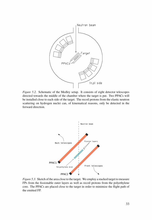
Figure 5.2. Schematic of the Medley setup. It consists of eight detector telescopesdirected towards the middle of the chamber where the target is put. Two PPACs willbe installed close to each side of the target. The recoil protons from the elastic neutronscattering on hydrogen nuclei can, of kinematical reasons, only be detected in theforward direction.

Figure 5.3. Sketch of the area close to the target. We employ a stacked target to measureFPs from the fissionable outer layers as well as recoil protons from the polyethylenecore. The PPACs are placed close to the target in order to minimize the flight path ofthe emitted FP.

33

5.2.1 Detector telescopesEach telescope consists of three independent detectors, chosen in order tobe able to detect light ions with the ΔE-ΔE-E technique. In the front ofeach telescope, facing the target, is a thin (50 μm), fully depleted, silicondetector. It is followed by another fully depleted silicon detector of similaror larger thickness. The third detector is a CsI(Tl) crystal optically coupledto a photodiode. It has to be thick enough to fully stop any particle that thetelescope measures. The aperture areas of the silicon detectors are 450mm2

each, which corresponds to about 20msr per telescope at a 15 cm distance.Because of the width of each telescope, all eight telescopes cannot be fittedinto the chamber if a smaller distance than 15 cm is used. A larger distance, upto about 30 cm, is possible but with a smaller solid angle as a result. A photoof one of the telescopes was shown previously in fig. 3.4.

The telescope angles are, under normal circumstances, fixed with respect toeach other. However, the whole setup of eight telescopes can be collectivelyrotated in order to cover other angles or to estimate systematic uncertaintiesby rotating it 180°. Our ‘standard’ setup has the telescopes positioned at 20°intervals and the smallest angle covered by it is 20°.

We will also use the telescope detectors to detect FPs, but in that case thefront detectors will not be penetrated, but instead fully stop the FPs. Similarlyto how the recombination causes PHD due to the plasma effects in the silicondetectors (section 3.4.2), nuclear reactions in the CsI detectors can cause theincoming light ions to seemingly deposit less than their full energy in thedetector. This effect has been studied before and was shown to be less than 2%for 40MeV protons [69]. It was also found, in the same study, that the effectcan be precisely reproduced by simulations and therefore corrections for thiscan be made.

The detection efficiency ε in Eq. 2.2 can be expressed as

ε =Ω

4π× εSi × εPPAC, (5.1)

where the first factor is the efficiency due to the covered solid angle,Ω, and εxis the detector efficiency for detecting the impinging particle in the specifieddetector (PPACs are only applicable in the case of detecting FPs). For chargedparticles, energetic enough to leave a clear signal above the noise level, εSi ≈ 1.To first order, the solid angle for detecting FPs and for detecting the recoilprotons from elastic scattering is the same. It is only dependent on the silicondetector aperture and the distance to the target. However, since FPs have a veryhigh linear energy loss in solid materials, there is a possibility of an energydependent decrease of the active detector area due to, e.g., the presence ofglueing near the edges of the silicon surfaces. The extent, if any, of this effectwill be investigated using a californium source.

34

5.2.2 Stacked targetIn order for Eq. 2.2 to be valid, the flux φ of the cross section measurementmust be the same as the one of the reference measurement. The best wayof assuring this is to measure both cross sections simultaneously using thesame flux. Since this experiment will employ the same silicon detectors for allparticle detection we also need to place suitable targets for both the fission andthe elastic scattering in the chamber centre. We intend to construct a stackedtarget consisting of three separate targets. A polyethylene target in the middleand 235U/238U on each side of the polyethylene (see Fig. 5.3). Each targetwill have a diameter of 2.5 cm. The idea is that the deep penetrating protonsproduced in the mid-segment will escape the target assembly with only minorenergy losses.

If all layers of the target are made modular, one could put together any mixof two outer fission layers and different thicknesses of the centre polyethylenelayers (or none at all). The fission target will have thin backings so thatboth fragments can be detected if no polyethylene is in use. Consideringthe expected neutron flux, target diameter and the solid angle covered by thesilicon detectors, a fission count rate of at least 1 kHz per μm of fissionabletarget thickness is anticipated.

5.2.3 Neutron energyThe energy of an incoming neutron will be determined using the time elapsedbetween the arrival of the primary beam bunch at the production target andthe detection of the first reaction product. This detected time tdet is a sum ofthe neutron ToF tn and the ToF of the charged secondary particle between thetarget and the detection point tp. That is,

tdet = tn + tp. (5.2)

From the information we get when detecting the secondary particle we mustbe able to deduce the neutron ToF with low uncertainty, in order to allow foraccurate measurements. As long as the secondary particle species is known,as in the recoil proton case, determining the neutron energy from the ToFis straight forward. However, when a FP is measured in one of the silicondetectors, only time and energy information is available. To deduce a ToF forthe detected FP one would need more information, e.g. like the fragment massor a second time signal, in order to deduce the FP velocity. This is the reasonwe are upgrading our setup with PPACs.

PPACs are thin enough to allow FP to be transmitted through them (althoughwith some energy losses) and later be detected in the silicon detectors as well.The heavy ions are moving so slowly that even though the PPACs are placedwithin a centimetre of the target, a correction for the flight time between targetand PPAC needs to be performed. Since the FP speed between the PPAC and

35

the silicon detector is obtained, an approximate correction can be made byestimating the energy losses before detection in the silicon detector. Ideally,the PPAC is placed very close to the target.

5.2.4 Particle identificationSince an α-particle background from the uranium target is expected (bothneutron-induced and due to natural decay), one needs to clearly separate theseevents from fission events. Even though the FPs are much heavier than α-particles, some overlap between the FP and α-particle distributions was ex-pected in the energy spectrum from the PPACs [70] (but in section 5.4 we willsee that this was not the case). If needed, the separation was supposed to beassisted by information from the silicon detectors in the overlap region.

A 50 μm silicon detector will fully stopα-particles of up to about 8MeV (theα-particle punch-through energy). Any transmitted α-particles will depositless than 8MeV in the detector due to the decrease in stopping power withenergy. The FPs, on the other hand, will always be fully stopped in the silicondetector and deposit their full energy. An α-particle discrimination is thuspossible by interpreting all particles depositing more than 8MeV as FPs. Forsuch a scheme to work, it would be imperative that the FPs do not lose too muchenergy before they reach, and are fully stopped in, the detector telescopes.

All particles, penetrating at least the front silicon detector, can be identifiedby the ΔE-ΔE-E technique (see section 3.4). The recoil protons from elasticscattering will not only be identified by the kinematical relationship betweenenergy and angle, but also through a distinct proton fingerprint in form of theenergy depositions in the different telescope detectors.

In addition to simulating the 235U(n,f) versus 238U(n,f) versus H(n,n) meas-urement, the same simulation software was used to simulate LCP on varioustargets, e.g. Si. As an example of the ΔE-ΔE-E technique, the plot in Fig. 5.4shows simulatedΔE-ΔE events. In this plot, the proton, deuteron and triton dis-tributions bend backwards as the particle energies exceed the particle-specificpunch-through energy of the second detector (in this case, 500 μm thick). Byhaving three detectors in the telescope, these higher energy events can still beseparated using the information from the last detector.

5.2.5 ObservablesWhile the angular integrated fission cross sections of 238U and 235U measuredrelative to the H(n,n) cross section, as well as against each other, are themain expected outcomes of this experiment, additional observables can beextracted. Each fission cross section is in fact measured at several differentangles. In order to integrate these data points into the angular integratedcross section, one must interpolate and extrapolate into the angular region not

36

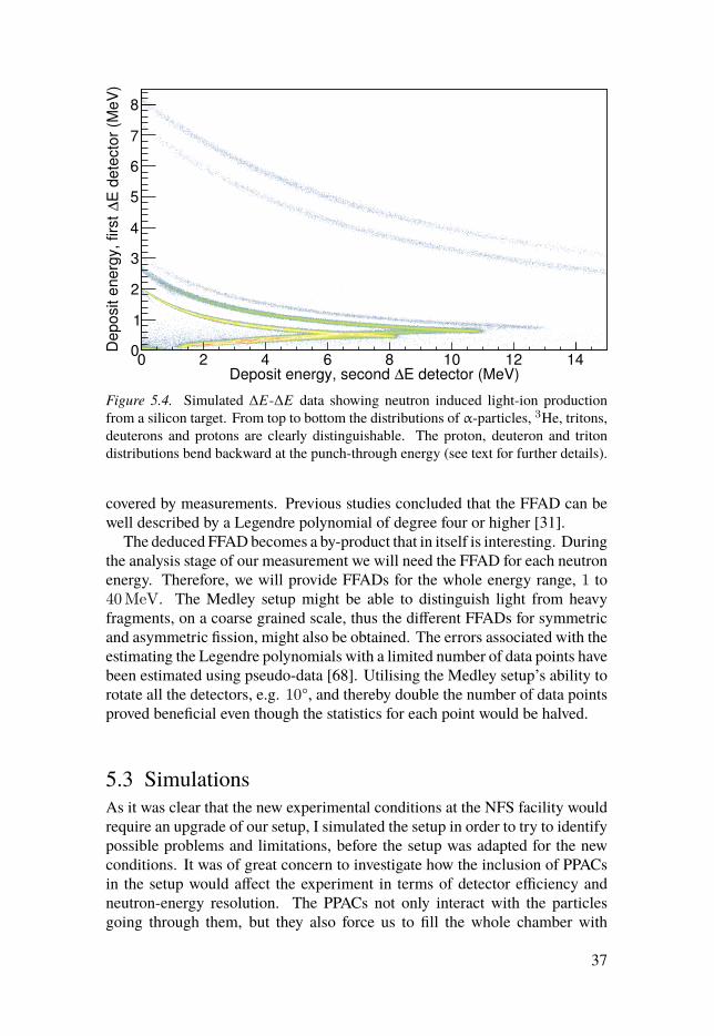
E detector (MeV)ΔDeposit energy, second 0 2 4 6 8 10 12 14

E d

ete

cto

r (M

eV

)Δ

De

po

sit e

ne

rgy,

firs

t

0

1

2

3

4

5

6

7

8

Figure 5.4. Simulated ΔE-ΔE data showing neutron induced light-ion productionfrom a silicon target. From top to bottom the distributions of α-particles, 3He, tritons,deuterons and protons are clearly distinguishable. The proton, deuteron and tritondistributions bend backward at the punch-through energy (see text for further details).

covered by measurements. Previous studies concluded that the FFAD can bewell described by a Legendre polynomial of degree four or higher [31].

The deduced FFAD becomes a by-product that in itself is interesting. Duringthe analysis stage of our measurement we will need the FFAD for each neutronenergy. Therefore, we will provide FFADs for the whole energy range, 1 to40MeV. The Medley setup might be able to distinguish light from heavyfragments, on a coarse grained scale, thus the different FFADs for symmetricand asymmetric fission, might also be obtained. The errors associated with theestimating the Legendre polynomials with a limited number of data points havebeen estimated using pseudo-data [68]. Utilising the Medley setup’s ability torotate all the detectors, e.g. 10°, and thereby double the number of data pointsproved beneficial even though the statistics for each point would be halved.

5.3 SimulationsAs it was clear that the new experimental conditions at the NFS facility wouldrequire an upgrade of our setup, I simulated the setup in order to try to identifypossible problems and limitations, before the setup was adapted for the newconditions. It was of great concern to investigate how the inclusion of PPACsin the setup would affect the experiment in terms of detector efficiency andneutron-energy resolution. The PPACs not only interact with the particlesgoing through them, but they also force us to fill the whole chamber with

37

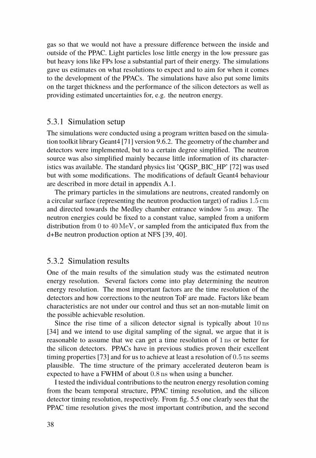
gas so that we would not have a pressure difference between the inside andoutside of the PPAC. Light particles lose little energy in the low pressure gasbut heavy ions like FPs lose a substantial part of their energy. The simulationsgave us estimates on what resolutions to expect and to aim for when it comesto the development of the PPACs. The simulations have also put some limitson the target thickness and the performance of the silicon detectors as well asproviding estimated uncertainties for, e.g. the neutron energy.

5.3.1 Simulation setupThe simulations were conducted using a program written based on the simula-tion toolkit library Geant4 [71] version 9.6.2. The geometry of the chamber anddetectors were implemented, but to a certain degree simplified. The neutronsource was also simplified mainly because little information of its character-istics was available. The standard physics list ’QGSP_BIC_HP’ [72] was usedbut with some modifications. The modifications of default Geant4 behaviourare described in more detail in appendix A.1.

The primary particles in the simulations are neutrons, created randomly ona circular surface (representing the neutron production target) of radius 1.5 cmand directed towards the Medley chamber entrance window 5m away. Theneutron energies could be fixed to a constant value, sampled from a uniformdistribution from 0 to 40MeV, or sampled from the anticipated flux from thed+Be neutron production option at NFS [39, 40].

5.3.2 Simulation resultsOne of the main results of the simulation study was the estimated neutronenergy resolution. Several factors come into play determining the neutronenergy resolution. The most important factors are the time resolution of thedetectors and how corrections to the neutron ToF are made. Factors like beamcharacteristics are not under our control and thus set an non-mutable limit onthe possible achievable resolution.

Since the rise time of a silicon detector signal is typically about 10 ns[34] and we intend to use digital sampling of the signal, we argue that it isreasonable to assume that we can get a time resolution of 1 ns or better forthe silicon detectors. PPACs have in previous studies proven their excellenttiming properties [73] and for us to achieve at least a resolution of 0.5 ns seemsplausible. The time structure of the primary accelerated deuteron beam isexpected to have a FWHM of about 0.8 ns when using a buncher.

I tested the individual contributions to the neutron energy resolution comingfrom the beam temporal structure, PPAC timing resolution, and the silicondetector timing resolution, respectively. From fig. 5.5 one clearly sees that thePPAC time resolution gives the most important contribution, and the second

38

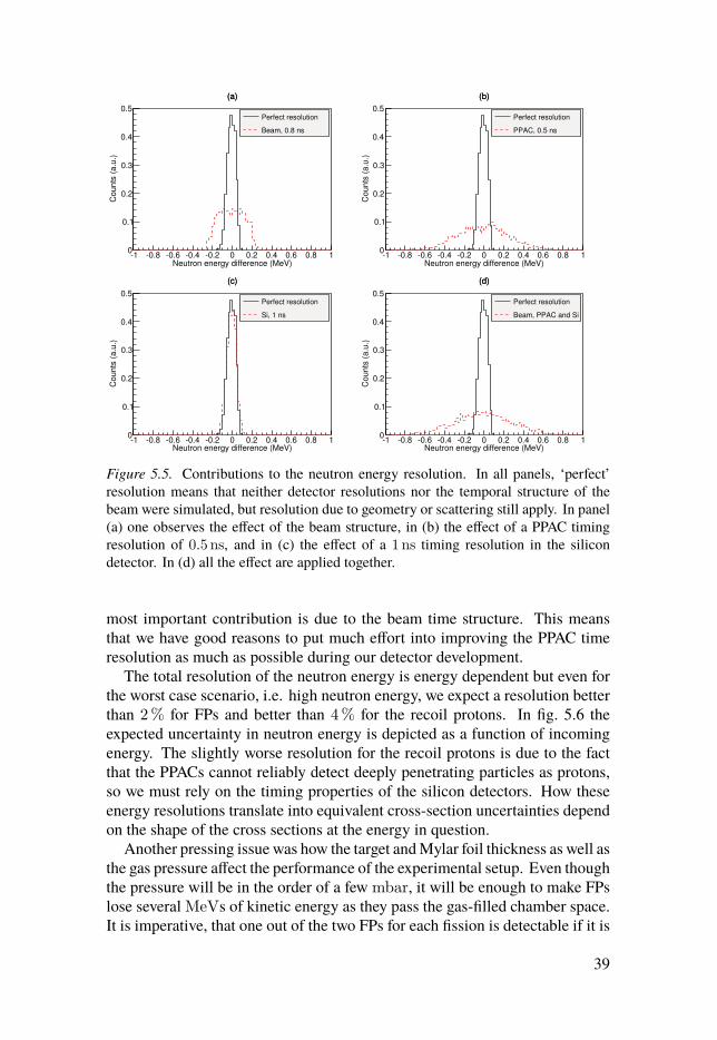
Neutron energy difference (MeV)-1 -0.8 -0.6 -0.4 -0.2 0 0.2 0.4 0.6 0.8 1

Co

un

ts (

a.u

.)

0

0.1

0.2

0.3

0.4

0.5

(a)

Perfect resolution

Beam, 0.8 ns

(a)

Neutron energy difference (MeV)-1 -0.8 -0.6 -0.4 -0.2 0 0.2 0.4 0.6 0.8 1

Co

un

ts (

a.u

.)

0

0.1

0.2

0.3

0.4

0.5

(b)

Perfect resolution

PPAC, 0.5 ns

(b)

Neutron energy difference (MeV)-1 -0.8 -0.6 -0.4 -0.2 0 0.2 0.4 0.6 0.8 1

Co

un

ts (

a.u

.)

0

0.1

0.2

0.3

0.4

0.5

(c)

Perfect resolution

Si, 1 ns

(c)

Neutron energy difference (MeV)-1 -0.8 -0.6 -0.4 -0.2 0 0.2 0.4 0.6 0.8 1

Co

un

ts (

a.u

.)

0

0.1

0.2

0.3

0.4

0.5

(d)

Perfect resolution

Beam, PPAC and Si

(d)

Figure 5.5. Contributions to the neutron energy resolution. In all panels, ‘perfect’resolution means that neither detector resolutions nor the temporal structure of thebeam were simulated, but resolution due to geometry or scattering still apply. In panel(a) one observes the effect of the beam structure, in (b) the effect of a PPAC timingresolution of 0.5 ns, and in (c) the effect of a 1 ns timing resolution in the silicondetector. In (d) all the effect are applied together.

most important contribution is due to the beam time structure. This meansthat we have good reasons to put much effort into improving the PPAC timeresolution as much as possible during our detector development.

The total resolution of the neutron energy is energy dependent but even forthe worst case scenario, i.e. high neutron energy, we expect a resolution betterthan 2% for FPs and better than 4% for the recoil protons. In fig. 5.6 theexpected uncertainty in neutron energy is depicted as a function of incomingenergy. The slightly worse resolution for the recoil protons is due to the factthat the PPACs cannot reliably detect deeply penetrating particles as protons,so we must rely on the timing properties of the silicon detectors. How theseenergy resolutions translate into equivalent cross-section uncertainties dependon the shape of the cross sections at the energy in question.

Another pressing issue was how the target and Mylar foil thickness as well asthe gas pressure affect the performance of the experimental setup. Even thoughthe pressure will be in the order of a few mbar, it will be enough to make FPslose several MeVs of kinetic energy as they pass the gas-filled chamber space.It is imperative, that one out of the two FPs for each fission is detectable if it is

39

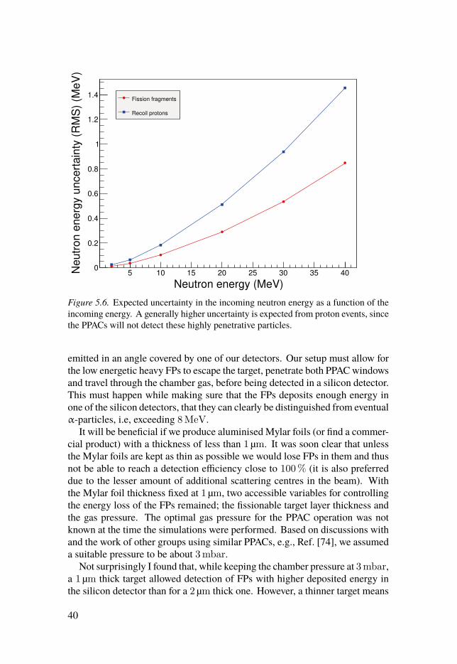
Neutron energy (MeV)5 10 15 20 25 30 35 40N

eutr

on e

nerg

y u

ncert

ain

ty (

RM

S)

(MeV

)

0

0.2

0.4

0.6

0.8

1

1.2

1.4Fission fragments

Recoil protons

Figure 5.6. Expected uncertainty in the incoming neutron energy as a function of theincoming energy. A generally higher uncertainty is expected from proton events, sincethe PPACs will not detect these highly penetrative particles.

emitted in an angle covered by one of our detectors. Our setup must allow forthe low energetic heavy FPs to escape the target, penetrate both PPAC windowsand travel through the chamber gas, before being detected in a silicon detector.This must happen while making sure that the FPs deposits enough energy inone of the silicon detectors, that they can clearly be distinguished from eventualα-particles, i.e, exceeding 8MeV.

It will be beneficial if we produce aluminised Mylar foils (or find a commer-cial product) with a thickness of less than 1 μm. It was soon clear that unlessthe Mylar foils are kept as thin as possible we would lose FPs in them and thusnot be able to reach a detection efficiency close to 100% (it is also preferreddue to the lesser amount of additional scattering centres in the beam). Withthe Mylar foil thickness fixed at 1 μm, two accessible variables for controllingthe energy loss of the FPs remained; the fissionable target layer thickness andthe gas pressure. The optimal gas pressure for the PPAC operation was notknown at the time the simulations were performed. Based on discussions withand the work of other groups using similar PPACs, e.g., Ref. [74], we assumeda suitable pressure to be about 3mbar.

Not surprisingly I found that, while keeping the chamber pressure at 3mbar,a 1 μm thick target allowed detection of FPs with higher deposited energy inthe silicon detector than for a 2 μm thick one. However, a thinner target means

40

Threshold energy (MeV)

0 2 4 6 8 10 12 14

Fra

ction b

elo

w thre

shold

energ

y

0

0.002

0.004

0.006

0.008

0.01

m targetμ1 mbar pressure, 2

m targetμ3 mbar pressure, 1

m targetμ3 mbar pressure, 2

Figure 5.7. The fraction of FPs that reach the front silicon detector with energy lowerthan the threshold is indicated on the x-axis. Most of the fragment’s kinetic energy islost while escaping the target and penetrating the PPAC foils as well as traversing thegas towards the detector telescopes. The PPAC foil thickness is kept at 1 μm. If thegas pressure is kept at 1mbar and the target is 2 μm thick, about 99.8% of the FPs aredetected with energies higher than 8MeV. To detect more FPs above the α-punch-through energy, the target thickness can be decreased to 1 μm allowing almost everyFP to reach the silicon detector with a kinetic energy above 8MeV.

lower count rate. If a lower gas pressure of 1mbar is used the 2 μm thick targetmight still be an option, letting us detect FPs with at least 8MeV in the silicondetector. The option of 3mbar gas pressure and a 2 μm thick target wouldtheoretically deny us the possibility to distinguish FP from α-particles by thepulse height in the silicon detector alone. The fraction of FP detected in thesilicon detector, above a certain threshold energy, is depicted in Fig. 5.7.

Considering PPAC windows of 1 μm one can estimate the additional scatter-ing centres for elastic scattering. Since we will measure the elastic scatteringfrom the polyethylene target, any extra hydrogen atoms in the beam must becorrected for. Depending on the final design of the PPACs and the relativethicknesses of the Mylar foils as well as of the polyethylene target, this cor-rection will be in the order of a few percent. It will be based on simulationstogether with empty target runs.

41

5.4 Current statusThe simulations and the analysis of them were performed mainly during 2013.Since then, PPACs have been built and tested in our laboratory in Uppsala usinga californium source. It turns out that with a 3mbar gas pressure the PPACs areessentially blind to α-particles but could still achieve a 100% efficiency for FPdetection (within experimental uncertainties) [68]. However, using the latestprototype PPAC a near 100% α-particle-efficiency was achieved at 7mbar.The final gas pressure and PPAC design will determine whether distinguishingFPs from α-particles will be problematic or not.

The specifications of the uranium targets are better known. In the simulationsthe uranium targets were modelled as uranium oxide but the real targets willmost likely be uranium tetra fluoride. They will also be thinner, in the order of0.5 μm, than the ones modelled in the simulations. All of these things play inour favour, increasing the margins for a working setup. The Mylar thickness isnow slightly less critical, but the energy losses must still be kept low. PPACswith window thicknesses of 2.5 μm were tested first, but now PPACs with0.9 μm windows have been produced and are currently being evaluated.

The simulations have helped the discussion and development of the exper-iment, but the situation is now changed. We have learned more and have abetter picture of the experiment we are planning. New simulations are plannedwhich calls for the simulation software to be updated and improved in order totake into account the current situation and the new information available. Themeasurements made using a 252Cf source with prototype PPACs (see fig. 3.3)[68] can now be compared to simulations. The work of updating the simula-tions is in the writing moment in progress. Due to the many delays of the NFSfacility, no experiments have yet been performed. Measurements of light-ionproduction is planned as soon as the neutron facility becomes operational andcommissioning will start.

42

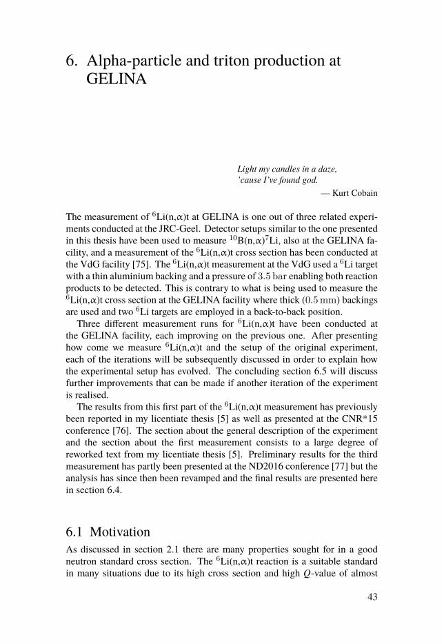
6. Alpha-particle and triton production atGELINA

Light my candles in a daze,’cause I’ve found god.

— Kurt Cobain

The measurement of 6Li(n,α)t at GELINA is one out of three related experi-ments conducted at the JRC-Geel. Detector setups similar to the one presentedin this thesis have been used to measure 10B(n,α)7Li, also at the GELINA fa-cility, and a measurement of the 6Li(n,α)t cross section has been conducted atthe VdG facility [75]. The 6Li(n,α)t measurement at the VdG used a 6Li targetwith a thin aluminium backing and a pressure of 3.5 bar enabling both reactionproducts to be detected. This is contrary to what is being used to measure the6Li(n,α)t cross section at the GELINA facility where thick (0.5mm) backingsare used and two 6Li targets are employed in a back-to-back position.

Three different measurement runs for 6Li(n,α)t have been conducted atthe GELINA facility, each improving on the previous one. After presentinghow come we measure 6Li(n,α)t and the setup of the original experiment,each of the iterations will be subsequently discussed in order to explain howthe experimental setup has evolved. The concluding section 6.5 will discussfurther improvements that can be made if another iteration of the experimentis realised.

The results from this first part of the 6Li(n,α)t measurement has previouslybeen reported in my licentiate thesis [5] as well as presented at the CNR*15conference [76]. The section about the general description of the experimentand the section about the first measurement consists to a large degree ofreworked text from my licentiate thesis [5]. Preliminary results for the thirdmeasurement has partly been presented at the ND2016 conference [77] but theanalysis has since then been revamped and the final results are presented herein section 6.4.

6.1 MotivationAs discussed in section 2.1 there are many properties sought for in a goodneutron standard cross section. The 6Li(n,α)t reaction is a suitable standardin many situations due to its high cross section and high Q-value of almost

43

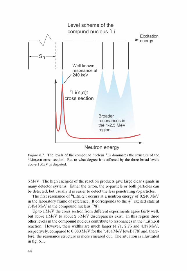
Figure 6.1. The levels of the compound nucleus 7Li dominates the structure of the6Li(n,α)t cross section. But to what degree it is affected by the three broad levelsabove 1MeV is disputed.

5MeV. The high energies of the reaction products give large clear signals inmany detector systems. Either the triton, the α-particle or both particles canbe detected, but usually it is easier to detect the less penetrating α-particles.

The first resonance of 6Li(n,α)t occurs at a neutron energy of 0.240MeVin the laboratory frame of reference. It corresponds to the 5

2

− excited state at7.454MeV in the compound nucleus [78].

Up to 1MeV the cross section from different experiments agree fairly well,but above 1MeV to about 2.5MeV discrepancies exist. In this region threeother levels in the compound nucleus contribute to resonances in the 6Li(n,α)treaction. However, their widths are much larger (4.71, 2.75 and 4.37MeV,respectively, compared to 0.080MeV for the 7.454MeV level) [78] and, there-fore, the resonance structure is more smeared out. The situation is illustratedin fig. 6.1.

44

In the 1 to 2.5MeV region at least two independent experiments havereported discrepancies. One experiment was performed using an ionisationchamber similar to the one used at JRC-Geel (see section 3.1) [79], while thesecond one employed solid state detectors [80]. Both experiments see a severalpercent higher cross section than, e.g., the ENDF/B-VII evaluation [81] in thisenergy region.

It is speculated [82] that one of the reasons the evaluation based on previousmeasurements shows a smaller cross section is the particle leaking effect. Dueto the incoming neutron momentum there is a possibility of both products(t and α) being emitted in the forward direction (in the laboratory frame ofreference), but with large polar angles (0° < θ < 90°) for moderate neutronenergies. In this case the detector response will look like as if only one particle,with the combined energy of both the triton and the α-particle, has entered thechamber. If this effect is overlooked it can lead to an underestimation of thecross section since the pulse height is much higher than for a normal α-particleevent and might be discarded because of that. This is why the effect is calledparticle leaking.

The aim of the study is to allow for an extension of the standard energy rangefrom 1MeV to a few MeV. Therefore, any discrepancies in this region mustbe resolved before the cross section can be trusted as a standard. An attemptto do this has been carried out by measuring the α-particles (and later alsothe tritons) from the 6Li(n,α)t reaction as well as the fission products from the235U(n,f) reference reaction.

6.2 First experimentData collection for the first iteration of this experiment started in spring 2015.

6.2.1 Experimental setupThe original experimental setup was situated at GELINA viewing the neutronproduction target unmoderated from a distance of 60m.

A schematic view of our GIC is depicted in fig. 6.2. This kind of detector wasdescribed in more detail in section 3.1. Contrary to most setups this chambercontained two cathodes, one for the lithium target and one for the uraniumtarget. The cylindrical chamber has one shared gas volume kept at a pressureslightly above 1 bar (the gas used was P-10), but the uranium measurement isconfined to the front compartment of the chamber and the lithium measurementto the back. Each compartment has a cathode in its centre and the uraniumand lithium targets, respectively, are placed on each side of the cathode so thateach pair of targets share the same cathode. In the case of the two uraniumtargets, a small 1.5mm spacer was inserted between the targets, but electricalcontact was still maintained.

45

Figure 6.2. Schematic of the ionisation chamber used for the first and second experi-mental runs. The chamber axis coincides with the neutron beam axis. Each cathodeconsists of two targets facing forwards respectively backwards. In total the chamberhas 10 independent electrodes, five in each compartment separated by shields. Theshields are interconnected and kept at the same potential.

Both lithium targets consisted of LiF, which was vacuum deposited on aaluminium backing and the deposited layers had similar masses, 2014(23)and 2610(40) μg, respectively. Both deposits had a diameter of 8 cm anda 0.5mm thick backing, making it impossible for any reaction products totraverse the target to the other side of the cathode (the range of a 5MeV tritonin aluminium is only about 100 μm [83]). The uranium targets were of similarareal densities, 193 and 222 μg/cm2, but due to different diameters (4.5 cm and7 cm, respectively) they had different masses, 3071(46) and 8520(40) μg 235U,respectively. The isotopic mass ratio of 235U in the uranium target materialwere 97.663(3) and 99.9336(14)% for the two targets, respectively.

On each side of each cathode, the chamber was equipped with an anode anda grid. The induced signals on each electrode were recorded by a 100MHzdigitiser, with 12 bits resolution. Signals from all electrodes were capturedrather than only from the cathodes and anodes, in order to reduce uncertaintiesdue to electronic drift [27]. In this experiment the grids consist of conductivemeshes (rather than parallel wires, which is another option).

6.2.2 Analysis procedureThis section will go through how to determine the neutron energy from theToF, how to extract the necessary information from the electrode signals, aswell as how the full dataset is analysed.

6.2.2.1 Trace analysisThe digital sampling of the waveforms enables corrections in the post-analysisand has shown to be superior to analogue equipment [27]. The collection ofstored waveforms needs to be iterated in order to extract the relevant informa-

46

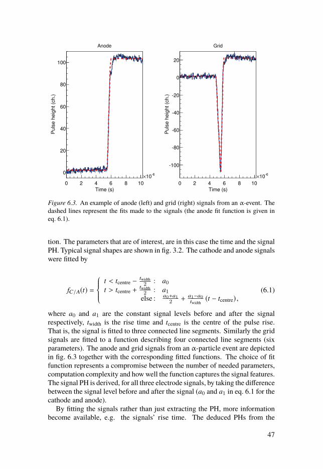
Time (s)

0 2 4 6 8 10

-610×

Pu

lse

he

igh

t (c

h.)

0

20

40

60

80

100

Anode

Time (s)

0 2 4 6 8 10

-610×

Pu

lse

he

igh

t (c

h.)

-100

-80

-60

-40

-20

0

20

Grid

Figure 6.3. An example of anode (left) and grid (right) signals from an α-event. Thedashed lines represent the fits made to the signals (the anode fit function is given ineq. 6.1).

tion. The parameters that are of interest, are in this case the time and the signalPH. Typical signal shapes are shown in fig. 3.2. The cathode and anode signalswere fitted by

fC/A(t) =⎧⎪⎪⎨⎪⎪⎩

t < tcentre − twidth2 : a0

t > tcentre +twidth2 : a1

else : a0+a12 +

a1−a0twidth

(t − tcentre) ,(6.1)

where a0 and a1 are the constant signal levels before and after the signalrespectively, twidth is the rise time and tcentre is the centre of the pulse rise.That is, the signal is fitted to three connected line segments. Similarly the gridsignals are fitted to a function describing four connected line segments (sixparameters). The anode and grid signals from an α-particle event are depictedin fig. 6.3 together with the corresponding fitted functions. The choice of fitfunction represents a compromise between the number of needed parameters,computation complexity and how well the function captures the signal features.The signal PH is derived, for all three electrode signals, by taking the differencebetween the signal level before and after the signal (a0 and a1 in eq. 6.1 for thecathode and anode).

By fitting the signals rather than just extracting the PH, more informationbecome available, e.g. the signals’ rise time. The deduced PHs from the

47

fitted signals were compared to the PHs obtained by applying a noise reducingCR-RC4 filter and then extracting the PH. No preference for either methodcould be seen. The χ2-distribution from the fit results corresponded to theexpected distribution considering the number of degrees of freedom as well asthe uncertainty (noise) of the baseline.

6.2.2.2 Time-of-flightThe trigger to the digitisers was created by letting each cathode signal gothrough pre-amplifier followed by a Constant Fraction Discriminator (CFD)and then adding them by a logical OR operation. The resulting signal wasthen combined by a logical AND operation with a signal from the controllingcomputer indicating whether the acquisition system is ready or not. The eventtime te, recorded for each event, is the time difference between this triggerand the accelerator signal arriving with each beam bunch. This timing can beturned into the ToF tToF, if a reference time t0 is known.

For calibration purposes bismuth and lead plates, with a total thickness of35mm and 15mm respectively, were placed in the neutron beam in front of thechamber during the measurements, in order for resonances to be visible in theToF spectrum. Neutrons with energies close to the resonances have a higherprobability of being absorbed before they reach the measurement chamber andtherefore negative peaks (a decrease of events) appear in the ToF spectrum atpredictable energies. If either the corresponding nuclear levels (see section 2.2for details) or the resonances themselves have been measured before, they canbe used as calibration points.

Except at energies below about a meV and at the resonance energies, thetotal neutron cross section of lead and bismuth is in the order of 10 b or lower[81]. This roughly corresponds to a neutron attenuation coefficient of lessthan 0.03 cm2/g. Compared to the attenuation coefficient for 5MeV γ’s [84]the neutron dito is significantly smaller, but in the same order of magnitude.The γ-attenuation decreases with γ-energy, so it is clear that these plates willattenuate low energetic γ-flux much more than the neutron flux. Therefore alower γ-background is achieved, at the expense of some neutron flux.

Unfortunately, even though previous experiments have used the same tech-nique [85, Fig. 1] and some resonances from the inserted beam filters werevisible, the resonances could not be unambiguously identified. Instead, theγ-flash coming from the neutron production target was used to determine thereference time t0. The peak in the ToF spectrum formed by γ-events, wasclearly separated from the events induced by slower particles. Since the speedof light is known,

tToF = te − t0 + L/c, (6.2)

where L is the distance between the neutron production target and the relevantcathode. Once the neutron ToF is deduced the kinetic energy of the neutron

48

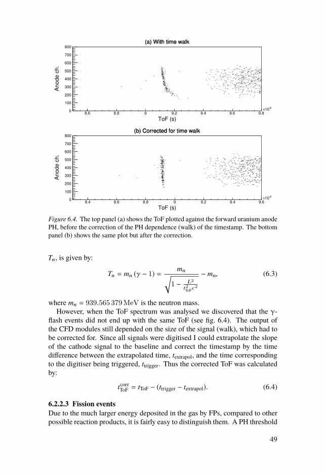
ToF (s)8.6 8.8 9 9.2 9.4 9.6 9.8

-610×

Anode c

h.

0

100

200

300

400

500

600

700

800(a) With time walk(a) With time walk

ToF (s)8.4 8.6 8.8 9 9.2 9.4 9.6

-610×

Anode c

h.

0

100

200

300

400

500

600

700

800(b) Corrected for time walk(b) Corrected for time walk

Figure 6.4. The top panel (a) shows the ToF plotted against the forward uranium anodePH, before the correction of the PH dependence (walk) of the timestamp. The bottompanel (b) shows the same plot but after the correction.

Tn, is given by:

Tn = mn (γ − 1) = mn√1 − L2

t2ToFc2

− mn, (6.3)

where mn = 939.565 379MeV is the neutron mass.However, when the ToF spectrum was analysed we discovered that the γ-

flash events did not end up with the same ToF (see fig. 6.4). The output ofthe CFD modules still depended on the size of the signal (walk), which had tobe corrected for. Since all signals were digitised I could extrapolate the slopeof the cathode signal to the baseline and correct the timestamp by the timedifference between the extrapolated time, textrapol, and the time correspondingto the digitiser being triggered, ttrigger. Thus the corrected ToF was calculatedby:

tcorrToF = tToF − (ttrigger − textrapol). (6.4)

6.2.2.3 Fission eventsDue to the much larger energy deposited in the gas by FPs, compared to otherpossible reaction products, it is fairly easy to distinguish them. A PH threshold

49

Grid ch.0 20 40 60 80 100 120

Anode c

h.

100

200

300

400

500

600

0G

1G

Figure 6.5. The anode PH plotted as a function of the anode PH, for all fission eventsin the forward direction. The lines represent the limits where the distribution heightdrops to half its maximum and defines cos θ = 0 and cos θ = 1.

separated the FPs unambiguously from the e.g. α-particles from the sampleactivity that were also present in the data. Due to the target and backingthickness, only one of the two FPs is detected for each fission event. The massof the FP is, for each single event, unknown and can only be estimated basedon its energy. The neutron energy does not reach more than a few MeV, soits influence on the fragment kinematics will be small. Due to this, all fissionevents emerging from the same side of the fission target are analysed together.In order to get the numbers of events in a specific neutron energy interval, anappropriate cut is applied later.

The analysis starts by plotting the anode signal PH versus the grid signal PHas in fig. 6.5. For each anode channel, corresponding to the detected energy,the fission events are projected onto the grid axis. The projection is used todetermine for which grid values the distribution drops to half its maximum.These grid values, G0 and G1, correspond to cos θ = 0 and cos θ = 1 (orcos θ = −1 for particles emerging from the backwards facing target). Wethen return to eq. 3.6 and remember that the grid PH is proportional to cos θ,allowing us to express cos θ as a function of the detected grid PH G(QG):

|cos θ | = G(QG) − G0

G1 − G0. (6.5)

The value of G0 is very close to zero since the FP emitted in the target planeshould not leave a net induced charge on the grid according to eq. 3.6. Thevalue of G1 will change with the fragment energy since it incorporates X whichin turn depends on the stopping range of the heavy ion in question. It turns outthat G1 can be well parametrised by two line segments as shown in fig. 6.5.

The fragments emitted in an angle close to 90◦ will suffer from larger energylosses in the target since the effective thickness of the target is proportional to1

cos θ . Corrections for the energy losses in the target can be made by observingthe mean energy of all events for a certain cosine value. The inverse cosine isplotted against the anode PH, denoted A, and a straight line, A = k

|cos θ | + m,

50

|θ1 / |cos 1 1.5 2 2.5 3 3.5

Anode c

h.

300

320

340

360

380

400

420

440

(a) Forward direction(a) Forward direction

|θ1 / |cos 1 1.5 2 2.5 3 3.5

Anode c

h.

300

320

340

360

380

400

420

440

(b) Backward direction(b) Backward direction

Figure 6.6. Mean anode PH plotted as a function of the inverse of the cosine value,for the fission events in both forward (a) and backward (b) direction. The fitted linesare used to correct for the angular dependent energy loss in the fission targets.

is fitted to the data where the losses are not too big (1.25 < 1cos θ < 3, see

fig. 6.6). We can estimate the anode PH, in the absence of energy loss in thetarget, with

Ano loss = A(θ) − k|cos θ | , (6.6)

through extrapolation of the fitted line by letting 1cos θ → 0. For gracing angles

the energy losses are too big to be well corrected for and some particle lossesare unavoidable. For the final analysis only the events where |cos θ | > 0.3 areused. The anode PH can be roughly translated into energy by calibrating theanode spectrum using the two distinct humps of light and heavy fragments,respectively.

6.2.2.4 α-particle eventsThe two reaction products (4He and 3H) are in this case of comparable massesto the neutron’s, which means that the kinematics are strongly dependent onboth the neutron energy and the emission angles in the laboratory frame ofreference. In the limiting case of an incoming neutron with negligible energy,

51

the angular distribution is isotropic and the α-particle and triton energies willbe determined only by the reaction’s Q-value together with the conservationof energy and momentum. In other words, the laboratory and the CoM frameare, in this case, identical.

For higher neutron energies difficulties arise. The two products will nolonger be emitted in opposite directions in the laboratory frame, due to themomentum transfer of the incoming neutron. The particle leaking has alreadybeen discussed in section 6.1. The particle energy is the largest at small angles,where it is also increasing with neutron energy. For backwards particle emis-sion the neutron momentum (qn) transfer will decrease the particle energies butat the same time the neutron energy (∝ q2

n), will increase the available reactionenergy. These two opposing effects lead to a non-monotonic behaviour of thebackwards emitted particle energies.

At this pressure of 1 bar, the tritons are not fully stopped in the chamber forsmall angles. Therefore, only the α-particles are of interest for this analysis.When the grid PH is plotted against the anode PH, the α-particle distributioncan be recognised as a fairly straight ’banana’ shape (see fig. 6.7). The distri-bution will move with neutron energy and the bent shape originates from boththe reaction kinematics as well as energy losses in the target. An increasedneutron energy will, for all forward angles, give rise to an increased particleenergy, leading to an increased anode PH. The energy losses in the target willalso change when the particle energy increases and therefore will the shapeof the distribution also change. The relevant distribution was selected usingmanual cuts for several neutron energies. These cuts were parametrised sothat the relevant events, of arbitrary neutron energies, could be selected. Thetritons that are stopped, are seen as a fairly horizontal distribution. Much ofthe background can be attributed to partly stopped tritons.

The particle energy can be determined both by calibrating the anode PHs,as well as by kinematic calculations based on the neutron energy derived fromthe ToF. The angles can be determined in a similar fashion as described forthe fission events. However, since in this case the neutron energy greatlyaffects the kinematics, the PH limits, G0 and G1, in eq. 6.5 must be determinedindependently for each small energy interval of interest.

The energy loss in the target does not scale linearly with particle energybut is generally small, except for gracing angles. An crude energy calibrationof the anodes can be performed by observing the events at the end points ofthe grid PH distribution. Since these corresponds to events of gracing anglesor events along the chamber axis, respectively, the corresponding laboratoryenergies are known. The anode PH of these events were used to create twoseparate energy calibrations, f cal

0 (A) and f cal±1 (A), each valid only for cos θ = 0

and cos θ = ±1, respectively. The laboratory energy could then be estimatedfor each event by interpolation between the two endpoint calibrations.

Elab = f cal±1 (A) |cos θ | + f cal

0 (A)(1 − |cos θ |) (6.7)

52

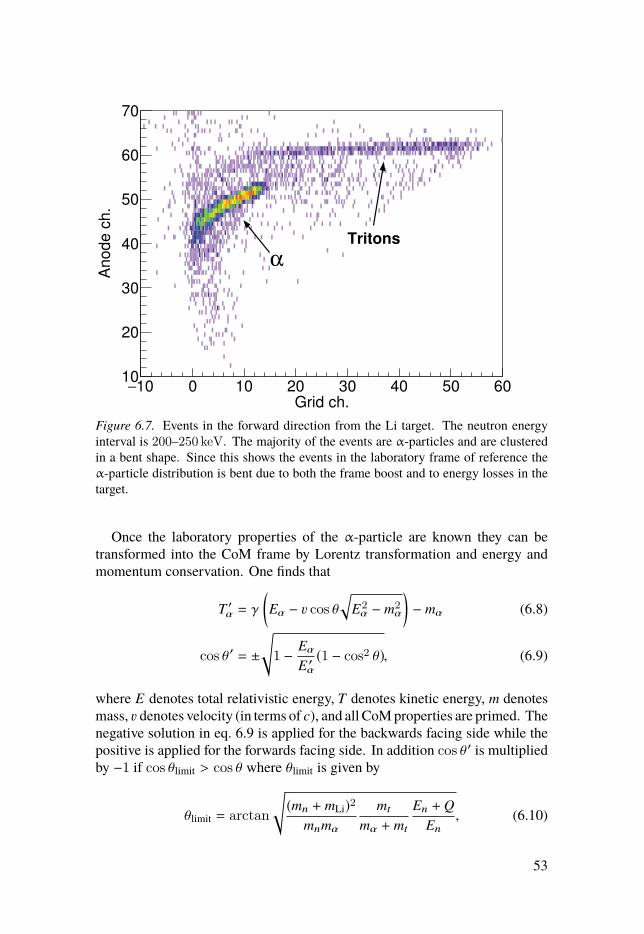
Grid ch.10− 0 10 20 30 40 50 60

Anod

e c

h.

10

20

30

40

50

60

70

α

Tritons

Figure 6.7. Events in the forward direction from the Li target. The neutron energyinterval is 200–250 keV. The majority of the events are α-particles and are clusteredin a bent shape. Since this shows the events in the laboratory frame of reference theα-particle distribution is bent due to both the frame boost and to energy losses in thetarget.

Once the laboratory properties of the α-particle are known they can betransformed into the CoM frame by Lorentz transformation and energy andmomentum conservation. One finds that

T ′α = γ

(Eα − � cos θ

√E2α − m2

α

)− mα (6.8)

cos θ ′ = ±√1 − Eα

E ′α(1 − cos2 θ), (6.9)

where E denotes total relativistic energy, T denotes kinetic energy, m denotesmass, � denotes velocity (in terms of c), and all CoM properties are primed. Thenegative solution in eq. 6.9 is applied for the backwards facing side while thepositive is applied for the forwards facing side. In addition cos θ ′ is multipliedby −1 if cos θlimit > cos θ where θlimit is given by

θlimit = arctan

√(mn + mLi)2

mnmα

mt

mα + mt

En +QEn

, (6.10)

53

Table 6.1. Ratios between fission event properties associated with the forward andbackward direction with respect to the beam. The detected counts and average linearenergy loss in the targets are compared to the expected values based on the targetspecifications. The relative difference between the measured and expected values arealso reported.

Property Ratio (f/b) Expected value Relative differenceEvent counts 2.741(14) 2.774(43) 1.2%Energy loss 1.20 1.15 4.7%

in order to take into account that the forward laboratory angle might havereached into the back hemisphere of the CoM frame.

6.2.3 Results6.2.3.1 Uranium counts and distributionsFor FP of gracing angles, the effective thickness of the target becomes large.Consequently, the energy losses will be large too, making accurate correctionsmore difficult. Sometimes the fragments will not even escape the target. Onecan see that some losses of events are occurring in the cosine spectra in fig. 6.8.

To avoid being affected by particle losses, only the fission events where|cos θ | > 0.3 were used. By comparing the ratio of event counts in the forwardand backward direction with the ratio of 235U atoms in the correspondingtargets, one can conclude that the relative number of detected events is veryclose to the expected (see table 6.1). Another check is to compare the energyloss (the slopes of the fitted lines in fig. 6.6, see eq. 6.6) with the targetthicknesses. Taking into account that the gain of the two different anodes aresimilar but not identical, the agreement between the measured value and theexpected is once again good (see table 6.1).

To be able to compare the anode distributions they were transformed intoenergy distributions by using the two peaks (corresponding to the low energyheavy fragments and the high energy light fragments, respectively) as calibra-tion points. Depicted in fig. 6.9 are the two energy spectra from the forward andbackward direction. They match each other well, but some small discrepancycan be seen at lower energies.

6.2.3.2 6Li(n,α)t in the centre-of-momentum frameFor each identified α event the laboratory properties were determined usingeq. 6.7 after deducing the angle from the grid PH. By subsequently usingeqs. 6.8 and 6.9 a transformation into the CoM frame was performed. Theresult is a distribution close to constant in energy (see fig. 6.10). The spreadof the distribution can be attributed to uncertainties in the neutron energyas well as in the particle angle. However, the deviation from the predicted

54

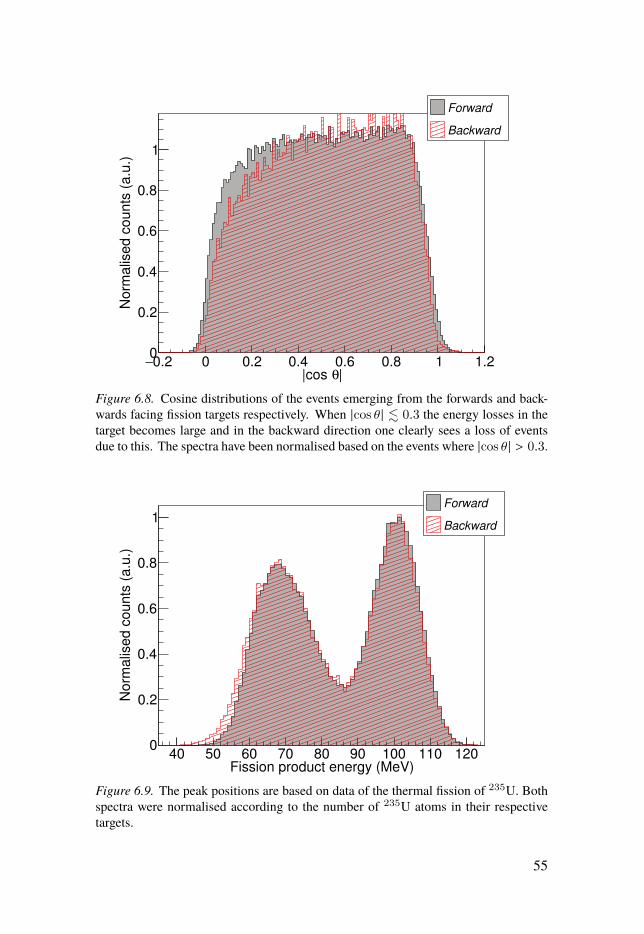
|θ|cos 0.2− 0 0.2 0.4 0.6 0.8 1 1.2

No

rma

lise

d c

ou

nts

(a

.u.)

0

0.2

0.4

0.6

0.8

1

Forward

Backward

Figure 6.8. Cosine distributions of the events emerging from the forwards and back-wards facing fission targets respectively. When |cos θ | � 0.3 the energy losses in thetarget becomes large and in the backward direction one clearly sees a loss of eventsdue to this. The spectra have been normalised based on the events where |cos θ | > 0.3.

Fission product energy (MeV)40 50 60 70 80 90 100 110 120

No

rma

lise

d c

ou

nts

(a

.u.)

0

0.2

0.4

0.6

0.8

1Forward

Backward

Figure 6.9. The peak positions are based on data of the thermal fission of 235U. Bothspectra were normalised according to the number of 235U atoms in their respectivetargets.

55

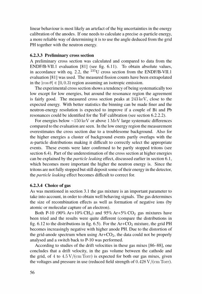
linear behaviour is most likely an artefact of the big uncertainties in the energycalibration of the anodes. If one needs to calculate a precise α-particle energy,a more reliable way of determining it is to use the angle deduced from the gridPH together with the neutron energy.

6.2.3.3 Preliminary cross sectionA preliminary cross section was calculated and compared to data from theENDF/B-VII.1 evaluation [81] (see fig. 6.11). To obtain absolute values,in accordance with eq. 2.2, the 235U cross section from the ENDF/B-VII.1evaluation [81] was used. The measured fission counts have been extrapolatedin the |cos θ | ∈ [0, 0.3) region assuming an isotropic emission.

The experimental cross section shows a tendency of being systematically toolow except for low energies, but around the resonance region the agreementis fairly good. The measured cross section peaks at 243 keV, close to theexpected energy. With better statistics the binning can be made finer and theneutron-energy resolution is expected to improve if a couple of Bi and Pbresonances could be identified for the ToF calibration (see section 6.2.2.2).

For energies below ∼150 keV or above 1MeV large systematic differencescompared to the evaluation are seen. In the low energy region the measurementoverestimates the cross section due to a troublesome background. Also forthe higher energies a cluster of background events partly overlaps with theα-particle distributions making it difficult to correctly select the appropriateevents. These events were later confirmed to be partly stopped tritons (seesection 6.4). Part of the underestimation of the cross section at higher energiescan be explained by the particle leaking effect, discussed earlier in section 6.1,which becomes more important the higher the neutron energy is. Since thetritons are not fully stopped but still deposit some of their energy in the detector,the particle leaking effect becomes difficult to correct for.

6.2.3.4 Choice of gasAs was mentioned in section 3.1 the gas mixture is an important parameter totake into account, in order to obtain well behaving signals. The gas determinesthe size of recombination effects as well as formation of negative ions (byatomic or molecular capture of an electron).

Both P-10 (90% Ar+10% CH4) and 95% Ar+5% CO2 gas mixtures havebeen tried and the results were quite different (compare the distributions infig. 6.12 to the distributions in fig. 6.5). For the Ar+CO2 mixture, the grid PHbecomes increasingly negative with higher anode PH. Due to the distortion ofthe grid-anode spectrum when using Ar+CO2, the data could not be properlyanalysed and a switch back to P-10 was performed.

According to studies of the drift velocities in these gas mixes [86–88], oneconcludes that a drift velocity, in the gas volume between the cathode andthe grid, of 4 to 4.5V/(cmTorr) is expected for both our gas mixes, giventhe voltages and pressure in use (reduced field strength of 0.428V/(cmTorr).

56

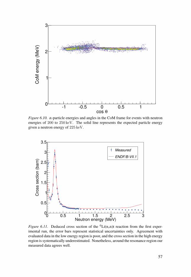
θcos -1 -0.5 0 0.5 1

CoM

energ

y (

MeV

)

0

1

2

3

Figure 6.10. α-particle energies and angles in the CoM frame for events with neutronenergies of 200 to 250 keV. The solid line represents the expected particle energygiven a neutron energy of 225 keV.

Neutron energy (MeV)0 0.5 1 1.5 2 2.5 3

Cro

ss s

ectio

n (

ba

rn)

0

0.5

1

1.5

2

2.5

3

3.5

Measured

ENDF/B-VII.1

Figure 6.11. Deduced cross section of the 6Li(n,α)t reaction from the first exper-imental run, the error bars represent statistical uncertainties only. Agreement withevaluated data in the low energy region is poor, and the cross section in the high energyregion is systematically underestimated. Nonetheless, around the resonance region ourmeasured data agrees well.

57

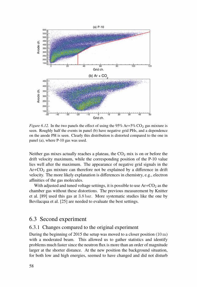
Figure 6.12. In the two panels the effect of using the 95% Ar+5% CO2 gas mixture isseen. Roughly half the events in panel (b) have negative grid PHs, and a dependenceon the anode PH is seen. Clearly this distribution is distorted compared to the one inpanel (a), where P-10 gas was used.

Neither gas mixes actually reaches a plateau, the CO2 mix is on or before thedrift velocity maximum, while the corresponding position of the P-10 valuelies well after the maximum. The appearance of negative grid signals in theAr+CO2 gas mixture can therefore not be explained by a difference in driftvelocity. The more likely explanation is differences in chemistry, e.g., electronaffinities of the gas molecules.

With adjusted and tuned voltage settings, it is possible to use Ar+CO2 as thechamber gas without these distortions. The previous measurement by Knitteret al. [89] used this gas at 3.8 bar. More systematic studies like the one byBevilacqua et al. [25] are needed to evaluate the best settings.

6.3 Second experiment6.3.1 Changes compared to the original experimentDuring the beginning of 2015 the setup was moved to a closer position (10m)with a moderated beam. This allowed us to gather statistics and identifyproblems much faster since the neutron flux is more than an order of magnitudelarger at the shorter distance. At the new position the background situation,for both low and high energies, seemed to have changed and did not disturb

58

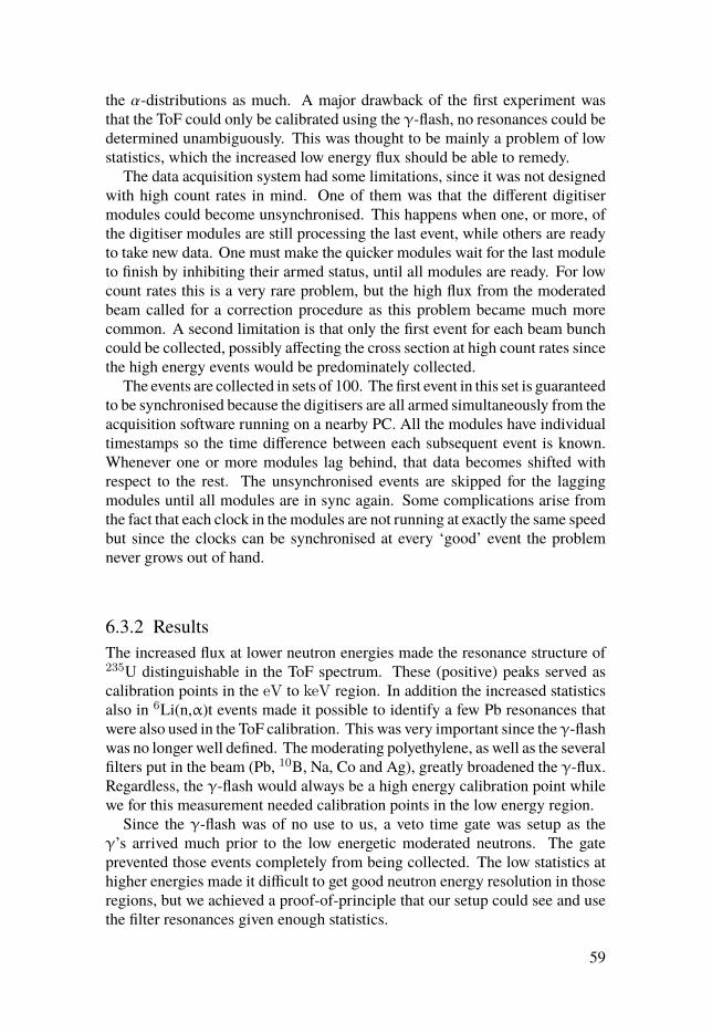
the α-distributions as much. A major drawback of the first experiment wasthat the ToF could only be calibrated using the γ-flash, no resonances could bedetermined unambiguously. This was thought to be mainly a problem of lowstatistics, which the increased low energy flux should be able to remedy.

The data acquisition system had some limitations, since it was not designedwith high count rates in mind. One of them was that the different digitisermodules could become unsynchronised. This happens when one, or more, ofthe digitiser modules are still processing the last event, while others are readyto take new data. One must make the quicker modules wait for the last moduleto finish by inhibiting their armed status, until all modules are ready. For lowcount rates this is a very rare problem, but the high flux from the moderatedbeam called for a correction procedure as this problem became much morecommon. A second limitation is that only the first event for each beam bunchcould be collected, possibly affecting the cross section at high count rates sincethe high energy events would be predominately collected.

The events are collected in sets of 100. The first event in this set is guaranteedto be synchronised because the digitisers are all armed simultaneously from theacquisition software running on a nearby PC. All the modules have individualtimestamps so the time difference between each subsequent event is known.Whenever one or more modules lag behind, that data becomes shifted withrespect to the rest. The unsynchronised events are skipped for the laggingmodules until all modules are in sync again. Some complications arise fromthe fact that each clock in the modules are not running at exactly the same speedbut since the clocks can be synchronised at every ‘good’ event the problemnever grows out of hand.

6.3.2 ResultsThe increased flux at lower neutron energies made the resonance structure of235U distinguishable in the ToF spectrum. These (positive) peaks served ascalibration points in the eV to keV region. In addition the increased statisticsalso in 6Li(n,α)t events made it possible to identify a few Pb resonances thatwere also used in the ToF calibration. This was very important since theγ-flashwas no longer well defined. The moderating polyethylene, as well as the severalfilters put in the beam (Pb, 10B, Na, Co and Ag), greatly broadened the γ-flux.Regardless, the γ-flash would always be a high energy calibration point whilewe for this measurement needed calibration points in the low energy region.

Since the γ-flash was of no use to us, a veto time gate was setup as theγ’s arrived much prior to the low energetic moderated neutrons. The gateprevented those events completely from being collected. The low statistics athigher energies made it difficult to get good neutron energy resolution in thoseregions, but we achieved a proof-of-principle that our setup could see and usethe filter resonances given enough statistics.

59

The data looked very promising but the deduced cross section was off, wehad too few fission events. After much of the beam time already had passed,it was discovered that the chamber was misaligned and that the neutron beamdid only illuminate part of the uranium targets.

The alignment is checked by taking photos of the beam. The γ’s in the beamwill react with the photo plate and after some hours you will see exactly wherethe beam hits your chamber. This was done before the measurement began butmost likely the chamber position was accidentally disturbed by, e.g., someonebumping into it or the table supporting it. Unfortunately this was impossibleto correct for in the analysis.

The last weeks of beam time was instead used to experiment with new highvoltage values and pressures. It had become apparent that the tritons were anunavoidable background. The often partly stopped tritons overlapped with theα-particle distribution. So we decided not to treat the tritons as backgroundand instead try to detect them as well by increasing the pressure.

In order to keep similar voltage ratios and reduced fields, the high voltagemust be increased proportionally to the increase in pressure which limitedus as the setup could not handle more than 3 kV. It was quickly seen thatdoubling the pressure reduced the triton background significantly, but at thecost of worsened performance for both α-particle and fission events, whichboth now experienced a shorter stopping range. Especially the grid resolutionwas worsened due to lower grid PHs. When the tritons were fully stopped, theparticle leaking could also be seen and these events counted, which was oneof the aims of the measurement.

The higher pressure seemed to be the way to go for the 6Li(n,α)t reactionbecause with measurable tritons theα-particle were no longer necessary. How-ever, a decent grid resolution is a must for the fission events in order to makethe energy correction. A decision was made to split the chamber into twochambers with different pressures before the next measurement.

6.4 Third experiment6.4.1 Changes compared to the second experimentThe lessons learned from both the previous experiments manifested into afew modifications. The first measurement struggled with low statistics due tothe long flight path of 60m while the second one, situated at 10m, only hadgood statistics for low energies due to the moderation. The third experimentended up at a distance of 30m from the unmoderated neutron production,a compromise of the two previous experiments. Previous measurements byKnitter et al. measured up to a neutron energy of 330 keV at that distance [89].

The chamber itself was split into two chambers, due to the decision madeat the end of the second experiment to employ different gas pressures for the

60

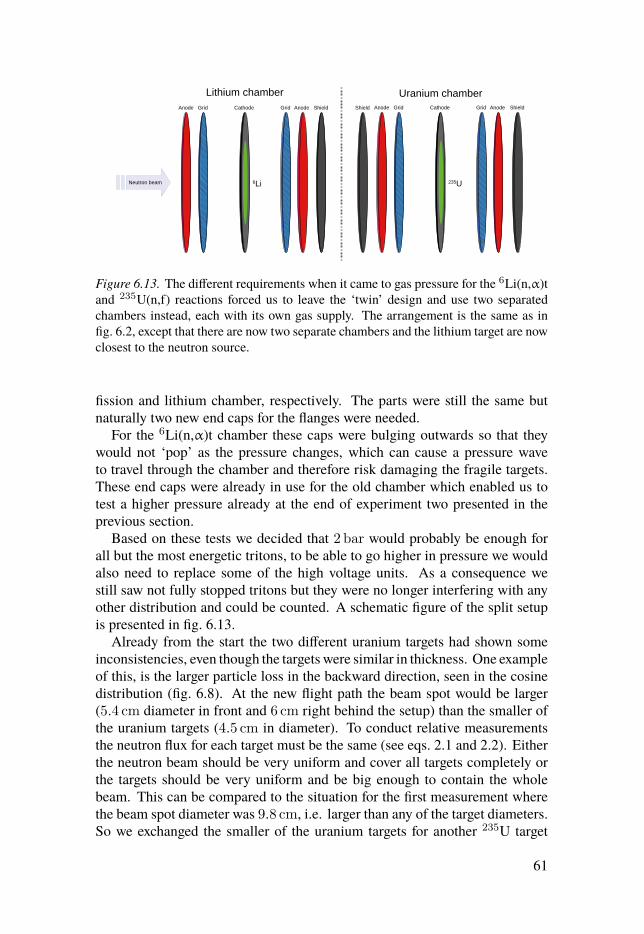
Figure 6.13. The different requirements when it came to gas pressure for the 6Li(n,α)tand 235U(n,f) reactions forced us to leave the ‘twin’ design and use two separatedchambers instead, each with its own gas supply. The arrangement is the same as infig. 6.2, except that there are now two separate chambers and the lithium target are nowclosest to the neutron source.

fission and lithium chamber, respectively. The parts were still the same butnaturally two new end caps for the flanges were needed.

For the 6Li(n,α)t chamber these caps were bulging outwards so that theywould not ‘pop’ as the pressure changes, which can cause a pressure waveto travel through the chamber and therefore risk damaging the fragile targets.These end caps were already in use for the old chamber which enabled us totest a higher pressure already at the end of experiment two presented in theprevious section.

Based on these tests we decided that 2 bar would probably be enough forall but the most energetic tritons, to be able to go higher in pressure we wouldalso need to replace some of the high voltage units. As a consequence westill saw not fully stopped tritons but they were no longer interfering with anyother distribution and could be counted. A schematic figure of the split setupis presented in fig. 6.13.

Already from the start the two different uranium targets had shown someinconsistencies, even though the targets were similar in thickness. One exampleof this, is the larger particle loss in the backward direction, seen in the cosinedistribution (fig. 6.8). At the new flight path the beam spot would be larger(5.4 cm diameter in front and 6 cm right behind the setup) than the smaller ofthe uranium targets (4.5 cm in diameter). To conduct relative measurementsthe neutron flux for each target must be the same (see eqs. 2.1 and 2.2). Eitherthe neutron beam should be very uniform and cover all targets completely orthe targets should be very uniform and be big enough to contain the wholebeam. This can be compared to the situation for the first measurement wherethe beam spot diameter was 9.8 cm, i.e. larger than any of the target diameters.So we exchanged the smaller of the uranium targets for another 235U target

61

with characteristics much more similar to the the large one already installed.The new target has an areal density of 216.0(16) μg/cm2, a diameter of 7 cmand a total 235U mass of 8310(4) μg with the same purity of 99.9336(14)%.

To fight the synchronisation issues found in the second run, the digitiserswere now supplied a common clock as time reference through a clock andtrigger distribution card.

We were running parasitically and the experiment in front of us neededa clean beam without filters. We planned to use some filters to get someresonances when the experiment in front of us was not taking data. However,as we started measuring, we immediately realised we were swamped by eventsinduced by the γ-flash. Even though our flight path was at an 108° angle to theprimary beam our chamber’s metallic beam window and other parts created alot of disturbing background and lots of space charges in our detector. Sinceour acquisition software could only handle one event per beam bunch it sohappened that without any veto gate, it triggered on the γ-flash every singletime. We made two adjustments to the setup to handle the situation.

The first adjustment was to extend our veto gate used in the previous exper-iment further, up to a time that roughly corresponded to a neutron energy of3MeV. Since no events were collected until this veto gate had ended, we hadto accept that we would never be able to measure any higher neutron energiesthat that, but we never expected to do so anyway. We also decided we couldnot measure without a beam filter, so 2 cm of lead was installed (the otherexperiment experienced problems and could not start in time). These twomeasures made it possible to run the experiment, and with the filters in placewe expected to see resonances to calibrate the ToF with.

The strong γ-flash also created a hassle to correctly fit the signals from the6Li(n,α)t reaction. In all events induced by neutrons of a few 100 keV or more,the signal trace would contain the γ-flash induced signal as well as the soughtfor one, piled up on the γ-event. The higher the energy of the impingingneutron, the shorter the distance between the γ-flash and the proper event. Acorrect fit is imperative to determine the PH, but also the signal rise time, sinceit is used to correct the ToF.

An algorithm was written that identified the γ-induced part of the signal andremoved it (see fig. 6.14). The identification was made based on an analysisof the ToF, PH and derivative. The anode channels had a much worse signalto noise ratio so the analysis of them were aided by the time information fromthe cathode (the onset of the anode signals are always later than the cathodesignal, see fig. 3.2).

Above a neutron energy of about 1MeV some of the 6Li(n,α)t events startedmerging completely with theγ-induced signal, why we had to discard the eventsof this energy or higher. In practice, only events below 0.5MeV yielded anyreasonable results.

62

Time / s1 2 3 4 5 6 7 8 9

6−

10×

Am

plit

ud

e /

ch

.

0

20

40

60

80

100

AnodeAnode

Time / s1 2 3 4 5 6 7 8 9

6−

10×

Am

plit

ud

e /

ch

.

20−

10−

0

102030

405060

GridGrid

Figure 6.14. Fitted signals of an event from the lithium chamber, which is highlyaffected by the γ-flash. The lower signal (black) in each panel have had the intervalaffected by the γ-flash removed from the original signal (red) before the fit (blue) wasmade.

6.4.2 ResultsExchanging the smaller uranium target not only resulted in a more consistentcross section, but also in a more consistent cosine distribution. Both distri-butions from the targets are now very similar with a flat top until the particlelosses for high angles kicks in (see fig. 6.15).

The improved statistics, compared to the first experimental run, made itpossible to unambiguously identify and use seven resonances from 208Pb forthe ToF calibration. The resonances covered the energy range 78 to 723 keV,which improved the overall ToF calibration.

In fig. 6.16 a typical situation for the lithium side of the chamber, at in-termediate (200 to 250 keV) neutron energies, is depicted. The α-particledistribution is now slightly more compressed since the pressure was increased.Some energy straggling is seen for angles close to 90° (grid channel ∼0).

The tritons are, for these energies, not fully stopped at near forward angles.Most of them are gathered in a straight distribution leaning upwards, in ac-cordance to the increased energy of forward directed particles. As the tritonsmanaged to pass through the whole gas volume and reach the anode, they startto deposit less energy in the cathode-anode region. The distribution bends at

63

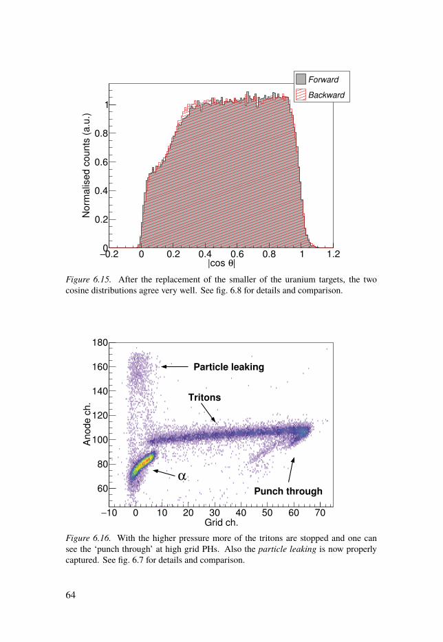
|θ|cos 0.2− 0 0.2 0.4 0.6 0.8 1 1.2

No

rma

lise

d c

ou

nts

(a

.u.)

0

0.2

0.4

0.6

0.8

1

Forward

Backward

Figure 6.15. After the replacement of the smaller of the uranium targets, the twocosine distributions agree very well. See fig. 6.8 for details and comparison.

Grid ch.10− 0 10 20 30 40 50 60 70

An

od

e c

h.

60

80

100

120

140

160

180

α

Tritons

Particle leaking

Punch through

Figure 6.16. With the higher pressure more of the tritons are stopped and one cansee the ‘punch through’ at high grid PHs. Also the particle leaking is now properlycaptured. See fig. 6.7 for details and comparison.

64

Neutron energy (MeV)0 0.1 0.2 0.3 0.4 0.5

Cro

ss s

ection (

barn

)

0

0.5

1

1.5

2

2.5

3

3.5

αMeasured

Measured tritons

ENDF/B-VII.1

Figure 6.17. Compared to the cross section presented in fig. 6.11, large improvementshave been made in the low energy region, and now both the tritons and α-particleshave been measured, yielding conforming results. However, the measured cross sectiondisagrees with the evaluation already after 300 keV, and despite much effort the dataabove a neutron energy of 0.5MeV could not be properly analysed due to the γ-flash.

a critical angle since the tritons are inducing less net charge on both the anodeand the grid.

For low angles, the triton distribution disappears and a cluster of events isformed at much energy. At these angles the particle leaking kicks in. Thecluster of events at high anode and low grid channels consists of simultaneousdetections of both reaction products, boosted into the forward hemisphere. Allthe distributions are almost completely separated and the background is verylow.

Increasing the pressure seem to have improved the situation since the back-ground is very low, and all distributions, including the punch through andparticle leaking effects, are accounted for. Alas, the deduced cross section infig. 6.17 still shows discrepancies, especially at energies higher than the first7Li resonance. At about 300 keV the γ-flash becomes increasingly difficultto handle and at energies above ∼500 keV the analysis failed to separate theevents properly.

Even if most of the γ-induced part of the signal is neutralised the ToF ofthe event is often affected. Another indication that the ToF calibration mightbe at fault, is that the the cross section deduced based on α-particles and

65

tritons, respectively, agree very well with each other at each energy point. Theexperimental cross section peaks before the cross section from ENDF/B-VII.1[81], which could be due to a misaligned ToF.

6.5 Improvements for a next experimentAfter each measurement, lessons were learned and the setup was improved.However, there are still many things that can be improved if a fourth measure-ment is attempted in the future.

6.5.1 DAQThe limit of one event per accelerator repetition is an unnecessary constraint.Upgrading the module that measures the time interval between the start and thestop signal, to a model that can handles several subsequent stop signals wouldremove this constraint completely.

The higher count rate, the more important it becomes that the timestamps ofthe digitisers can confirm that the traces from the different digitisers actuallydescribe the same event. Since the file structure was not aligned with the setstructure the events were collected in, and since a synchronisation correctionhad to be performed, the data analysis could not be trivially parallelised. Thisincreased either the time required for analysis or the complexity of the analysiscode.

In the third run, it still happened that some of the digitisers become unsyn-chronised. The only difference, compared to the second run, was that it waseasier to correct for, as all the digitisers used the same clock as a reference. Itdid not solve the fundamental problem of the unsynchronised events though.

6.5.2 γ-flashThe single biggest problem of the last measurements was the influence of theγ-flash. It limited the energy range we could measure and complicated theanalysis. Comparing the situations concerning the first and third experimentwe see the importance of enough beam filters to properly attenuate the γ-fluxto manageable levels. The increased flight length also helped by separating γand neutron events time wise.

Both these measures decrease the neutron flux as well as the γ flux, asan unwanted effect. As we saw that it was difficult to obtain well definedresonance dips in the ToF spectra, due to the low statistics at 60m, one wouldeither require much more beam time (and patience) or a shorter flight path. Anew measurement at about 30m with more beam filters (recall that the firstexperiment employed more than double the thickness than was used during

66

the third experiment) seems to be the most reasonable choice. A previousmeasurement by Knitter et al. at the same distance from the neutron sourceemployed 12 cm lead and 18 cm copper, and still experienced large γ-inducedsignals that limited the available energy range [89]. Thicker filters wouldalso deepen the resonances, leading to more of them being identified and themeasured position of them more accurate.

6.5.3 The lithium chamberThe increase in chamber pressure from 1 bar to 2 bar led to a major improve-ment for the measurement of both α-particles and tritons since their distri-butions no longer overlapped. The pressure was still a compromise though.The higher pressure decreased the angular resolution for the α-particles andincreased the energy loss drastically for events at close to 90° angles. On theother side, many of the tritons emerging from events of intermediate to highneutron energies at close to 0° angles were still only partially stopped in thegas. By accepting additional loss of performance for α-particles one couldincrease the pressure and focus on measuring tritons with good angular as wellas energy resolution. Care would still be need to make sure appropriate bias onthe electrodes can be supplied without causing sparks or ending up with fieldstrengths unfavourable with regards to the electron drift velocity in the gas.

67

7. Correlated fission observables with VERDI

When I saw you I fell in love, and yousmiled because you knew.

— Arrigo Boito

VERDI (VElocity foR Direct particle Identification) is a fission spectrometerdeveloped at the JRC-Geel. It is designed to measure correlated fission ob-servables through the 2E-2v method.

First results of the current design of VERDI was published by Frégeauet al. [90] at about the same time I joined the project. Since then the setuphas been upgraded and the analysis refined. Effort has also been put intobetter understanding the 2E-2v method in order to explain the results VERDIproduces, as well as guiding the continuation and development of the project.

I will focus on the 2E-2v method, but certain aspects of the 2E method willalso be relevant to discuss to some degree. A small part of this was presentedat the ND2016 conference [91], but here the current VERDI will be presentedand discussed in full for the first time.

7.1 MotivationStill, after almost 80 years since the discovery of fission we do not knowhow the fission process works in detail. One important question is how theavailable excitation energy is distributed between the two FFs. This can beprobed by measuring the neutron multiplicity, ν, since the ability to emit acertain number of neutrons requires enough excitation energy to pay for theneutrons’ separation energies. The multiplicity can be measured directly, butdetecting neutrons is always difficult. Instead one could measure the massof a fragment both before and after neutron emission and thereby deduce themultiplicity.

To help, or rule out, the developed theoretical models of fission, correlateddata is needed. If both the fragments’ masses and energies are known sim-ultaneously the correlations between them can say much more than a simpleone dimensional spectrum. Providing such correlated data is what VERDI hasbeen designed for. VERDI cannot provide correct correlations event-by-eventbut it can give average correlations between the masses, energies and otherdeducible observables.

Mass yields of higher quality than present measurements is also anticip-ated from VERDI, which could be interesting for applications like the nextgeneration nuclear power plants and transmutation technologies.

68

7.2 NotationThroughout this chapter there will be a lot of notation referring to differentquantities, often both before and after neutron emission. The, so called,pre-neutron and post-neutron quantities will be marked by superscript (pre orpost, respectively). The variables M , E , t and � will be used to representmass, kinetic energy, ToF and velocity (strictly speed), respectively. Directlymeasured uncorrected quantities will have a subscript (m) differentiating themfrom their corrected counterparts.

The symbol ν̄ denotes the average neutron multiplicity, for one of the frag-ments. The average total neutron multiplicity, summed over both fragments, isdenoted ν̄tot. If I need to specify that a quantity belongs to a specific fragment,the corresponding symbol will carry an index of either 1 or 2, while a quantitybelonging to a neutron has a subscript (n).

7.3 The 2E methodEven though VERDI is designed for 2E-2v measurements, the calibration ofthe setup depend on a 2E analysis of a well-known system, e.g., 252Cf(sf ).I will therefore briefly describe how the 2E method is implemented in theVERDI analysis, before I go through the main 2E-2v method.

As the name suggests the method is based on a measurement of both the FPs’energies. Since less information is obtained compared to a 2E-2v measure-ment, some previously obtained information is needed to deduce the fragmentmasses. In the following description it is assumed that there exists a func-tion ν̄(Mpre,TKEpre) that will provide the average neutron multiplicity givenMpre and TKEpre. In reality, such a function would be based on previousmeasurements of the same, or similar, fissioning systems.

The analysis of each event will undergo a couple of iterations in order toconverge toward the correct energies and masses. The kinetic energies of bothparticles is directly measured. The needed starting values of the other variablescan be set to, e.g.,

Eprei=0 = Epost (7.1)

Mpre1,i=0 = Msum

Epost2

Epost1 + Epost

2

, (7.2)

where Msum is explained in detail in section 7.4.2.

69

The next iterations will calculate the properties according to:

Mposti+1 = Mpre

i − ν̄(Mprei ,TKEpre

i ) (7.3)

Eprei+1 = Epost Mpre

i

Mposti+1

(7.4)

Mpre1,i+1 = Msum

Epre2,i+1

Epre1,i+1 + Epre

2,i+1

. (7.5)

When the variables have converged, usually within a few iterations, the loopis terminated and the analysis proceeds with the next event.

For each emitted neutron two terms have been neglected in eq. 7.4. Theexpression in eq. 7.4 comes from the assumption that �pre = �post. The size ofthis approximation can be determined by estimating the average values of boththe terms:

mnMpost ECoM

n and mn�pre�CoM

n .

The first term is small, in the order of tens of keVs, and the second termaverages to zero in the same manner as discussed in section 7.4.1. We willneed to come back and discuss these approximations later in section 7.7.5.

7.4 The 2E-2v methodTo utilise the 2E-2v method one needs to know the compound nucleus, i.e.,the fissioning system. The 2E-2v method is therefore only strictly valid forfirst-chance fission. However, for neutron energies high enough to enablemulti-chance fission [22], corrections can be made. Here, I restrict myself tofirst-chance fission.

As the name suggests the 2E-2v method relies on the measurement of theenergy and velocity of both FPs. Before I show how the energies and masses,both before and after neutron emission, are derived from this, an importantassumption needs to be clarified. All prompt neutrons are assumed to beemitted soon after the FFs become fully accelerated by the Coulomb repulsion.

7.4.1 Isotropic neutron emissionSince no neutrons are measured, the angular distribution must be estimatedsomehow. For both the 2E and 2E-2v methods, the neutron emission is assumedto be isotropic in the CoM frame of each individual fragment. I will nowdemonstrate why this assumption is imperative to the 2E-2v method.

Let us observe the system consisting of one of the FFs before neutronemission. Its momentum, Mpre�pre, is by definition along the fission axis. The

70

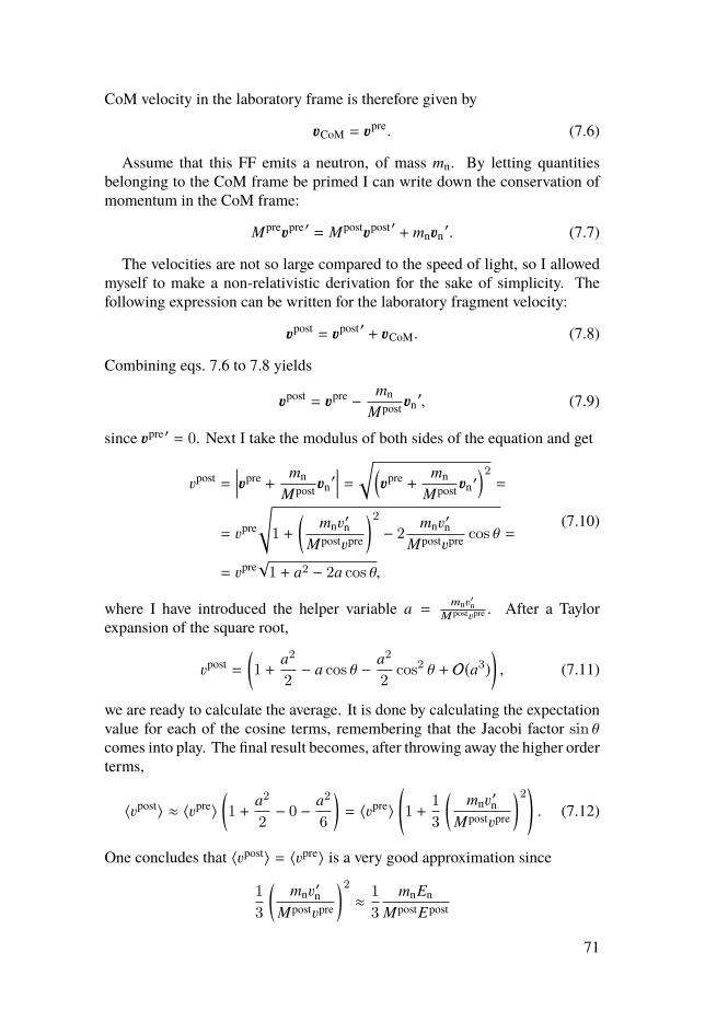
CoM velocity in the laboratory frame is therefore given by

�CoM = �pre. (7.6)

Assume that this FF emits a neutron, of mass mn. By letting quantitiesbelonging to the CoM frame be primed I can write down the conservation ofmomentum in the CoM frame:

Mpre�pre′ = Mpost�post′ + mn�n′. (7.7)

The velocities are not so large compared to the speed of light, so I allowedmyself to make a non-relativistic derivation for the sake of simplicity. Thefollowing expression can be written for the laboratory fragment velocity:

�post = �post′ + �CoM. (7.8)

Combining eqs. 7.6 to 7.8 yields

�post = �pre − mnMpost �n

′, (7.9)

since �pre′ = 0. Next I take the modulus of both sides of the equation and get

�post =����pre +

mnMpost �n

′��� =√(

�pre +mn

Mpost �n′)2=

= �pre

√1 +

(mn�

′n

Mpost�pre

)2− 2

mn�′n

Mpost�pre cos θ =

= �pre√1 + a2 − 2a cos θ,

(7.10)

where I have introduced the helper variable a = mn�′n

Mpost�pre . After a Taylorexpansion of the square root,

�post =

(1 +

a2

2− a cos θ − a2

2cos2 θ + O(a3)

), (7.11)

we are ready to calculate the average. It is done by calculating the expectationvalue for each of the cosine terms, remembering that the Jacobi factor sin θcomes into play. The final result becomes, after throwing away the higher orderterms,

〈�post〉 ≈ 〈�pre〉(1 +

a2

2− 0 − a2

6

)= 〈�pre〉

(1 +

1

3

(mn�

′n

Mpost�pre

)2). (7.12)

One concludes that 〈�post〉 = 〈�pre〉 is a very good approximation since

1

3

(mn�

′n

Mpost�pre

)2≈ 1

3

mnEnMpostEpost

71

evaluates to less than 0.01% for relevant masses and energies.In the whole 2E-2v analysis, �post is used as an approximation for the non-

measured �pre. In the case of 252Cf(sf ), estimating �pre by �post is approximatelyequivalent to a 1% normal distributed random error in �pre. This error translatesinto a pre-neutron mass resolution inherent to the method of about 0.8 amu.

7.4.2 Pre- and post-neutron masses and energiesFor every event the post-neutron energies are known from start, since they aredirectly measured along with the post-neutron velocities. The post-neutronmasses are easily calculated through

Mpost =Epost

γ − 1, (7.13)

where γ is the Lorentz factor. The difference between Newtonian and relativ-istic calculations is small, but doing it relativistically avoids a systematic errorin the order of 0.1 amu. The pre-neutron masses are determined by observingthe momentum conservation of the FFs, and using �pre ≈ �post:

Mpre1 �

post1 γ1 = Mpre

2 �post2 γ2 ⇔ Mpre

1 = Msum�

post2

�post1

γ1γ2+ �

post2

, (7.14)

where Msum = Mpre1 + Mpre

2 and γ2/γ1 ≈ 1.One can estimate Msum as the compound nucleus mass, MCN (for VERDI at

this stage, always the mass of 252Cf), but that will overestimate the pre-neutronmasses. The difference in binding energy goes into the kinetic energy of thefragments thus decreasing the mass of the full system. We can estimate TKEpre

classically by

TKEpre =MCN2�

post1 �

post2 , (7.15)

and thereby estimate Msum better:

Msum ≈ MCN − TKEpre = MCN

(1 − �

post1 �

post2

2

). (7.16)

With this approximation the systematic error is in the same order of mag-nitude as the excitation energies before neutron evaporation (tens of MeV, ora few percent of an atomic mass unit). Note that one does not ever actuallycalculate the rest masses since the fragments are, in general, excited after scis-sion. Also, one does not know exactly how many electrons are accompanyingthem.

72

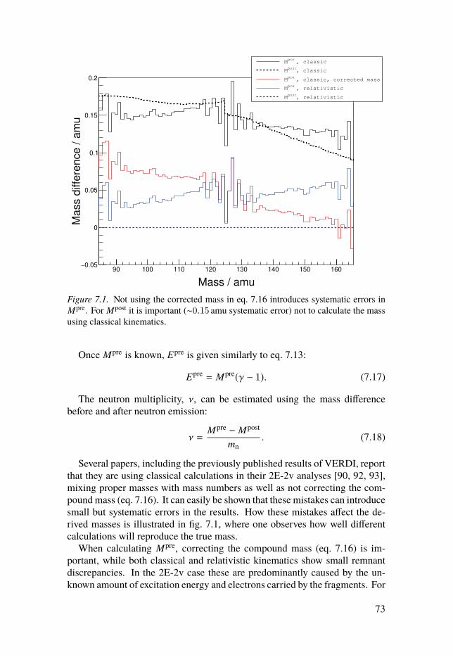
Mass / amu

90 100 110 120 130 140 150 160

Mass d

iffe

rence / a

mu

0.05−

0

0.05

0.1

0.15

0.2

, classicpre

M

, classicpost

M

, classic, corrected masspre

M

, relativisticpre

M

, relativisticpost

M

Figure 7.1. Not using the corrected mass in eq. 7.16 introduces systematic errors inMpre. For Mpost it is important (∼0.15 amu systematic error) not to calculate the massusing classical kinematics.

Once Mpre is known, Epre is given similarly to eq. 7.13:

Epre = Mpre(γ − 1). (7.17)

The neutron multiplicity, ν, can be estimated using the mass differencebefore and after neutron emission:

ν =Mpre − Mpost

mn. (7.18)

Several papers, including the previously published results of VERDI, reportthat they are using classical calculations in their 2E-2v analyses [90, 92, 93],mixing proper masses with mass numbers as well as not correcting the com-pound mass (eq. 7.16). It can easily be shown that these mistakes can introducesmall but systematic errors in the results. How these mistakes affect the de-rived masses is illustrated in fig. 7.1, where one observes how well differentcalculations will reproduce the true mass.

When calculating Mpre, correcting the compound mass (eq. 7.16) is im-portant, while both classical and relativistic kinematics show small remnantdiscrepancies. In the 2E-2v case these are predominantly caused by the un-known amount of excitation energy and electrons carried by the fragments. For

73

Figure 7.2. A not-to-scale sketch of the VERDI setup. The sputtered electrons (bluedotted lines) are directed toward the respective MCPs by electrostatic reflection in themirrors. The mirrors are mostly transparent to the FPs so that they can be detected inthe silicon detectors. A bent metallic structure shields the MCPs from direct radiationfrom the 252Cf source, it does not disrupt neither the electrons or FPs.

the Mpost calculation, it is clear that classical kinematics is inferior and shouldnot be used.

7.5 Experimental setupThe VERDI spectrometer, illustrated in fig. 7.2, consists of a vacuum chamberkept at an operating pressure of less than 1 × 10−7mbar. Keeping a lowpressure is necessary because of the two Multi Channel Plates (MCPs) thatdetects sputtered electrons from particles leaving the target. One MCP isplaced on each side of the target. Two electrostatic mirrors, each pairing upwith one of the MCPs, face the centred target at a 45° angle, reflecting theelectrons onto the respective MCP. A photo of one of the MCP assemblies, justa few moments before it was mounted inside the vacuum chamber, is shown infig. 7.3. In order to collect all electrons and steer them towards the mirror, anacceleration grid is positioned on each side, 4mm from the target.

32 silicon detectors are mounted on a spherical surface at about 0.5mdistance from the target. These form 16 detector pairs, facing each other inorder to be able to detect both FPs emerging from the target at a relative angleclose to 180°. Each of the silicon detectors has a circular surface area of450mm2. They are of the type Passivated Implanted Planar Silicon (PIPS)detectors which features thinner entrance windows and lower leakage currentsthan standard SSB detectors, but operates in a similar fashion.

74

Figure 7.3. One of the two MCP assemblies, moments before it was installed in theVERDI vacuum chamber. The whole assembly is mounted on a vacuum flange. Thecircular structure in the centre is the MCP, while the larger upper one is the electrostaticmirror.

The particle energies are measured by the silicon detectors which alsoprovide a stop signal for the ToF measurement. The start signal is providedby the sputtered electrons detected on the MCPs. No emission foils are used,enough electrons are emitted from the target itself. This minimises the energylosses of the FPs, which mainly lose energy in the target. The accelerationgrids as well as both the front and back planes of the electrostatic mirrorsconsist of parallel tungsten wires of 50 μm diameter at a 1mm pitch. The FPswill have to pass through both the acceleration grid and the mirror in order tobe detected in one of the silicon detectors. The total transparency for FPs is85.7%.

Both the acceleration grids and the front plane grids of the mirrors are keptat ground potential. The target itself is kept at −3 kV but due to the symmetricpositioning of the acceleration grids, no net force is put on the target. Thepotential of the back plane of the mirrors, −2950V, was chosen based on astudy of the detection efficiency of α-particles.

The MCPs are in a chevron configuration with the front kept at groundpotential and the back plane at 2.3 kV. The silicon detectors were all operatedfully depleted. Due to some being regular Passivated Implanted Planar Silicon(PIPS) detectors and others neutron transmuted PIPS detectors the required

75

voltages varied from 70 to 140V. No performance differences between thetwo different types of PIPS detectors have been noticed.

The silicon detector signals were fed into pre-amplifiers in a standard fash-ion. The energy signals were sent to an Analogue to Digital Converter (ADC)while the time signals were fed into a Constant Fraction Discriminator (CFD).A fission event will only trigger two opposing detectors, so at low count ratesonly two silicons detectors will have a signal at any given moment. There-fore, only one ADC in conjunction with a signal router was employed for eachside of VERDI. Each of the routers directs the active detector signal only, toits corresponding ADC. Similarly, the logical OR of all CFD channels werecoded into voltage levels by a Tag Word Coder (TWC) module before sent toan ADC. The timing signal from the MCP was fed into a Time to AnalogueConverter (TAC) together with the timing signal from the silicon detector ofthe corresponding side. The time difference gave rise to an output signal thatin turn was fed into an ADC. A complete scheme of the electronic setup isprovided in fig. 7.4.

The 252Cf(sf ) source had a 250 nm thick nickel backing. Unfortunately the252Cf migrates into the backing with time. By observing the different energylosses in events coming from the deposit and backing side, respectively, bothin the VERDI data as well as in previous experiments using the same target,an average depth of the 252Cf could be estimated to 62.5 nm. The fission ratewas in the order of 2 kHz.

Previously, VERDI had only one MCP installed on one side of the target.After the installation of the second MCP, improvements of the time resolutionwere expected. The ToF calibration improved, since it relied on detectingα-particles. The α-particles do not sputter many electrons in the oppositedirection of the α-particle’s movement. This was problematic when a MCPwas only available on one of the sides, i.e., the calibration of the opposing sidewas sub-optimal. With an MCP on each side, this is no longer a problem.

An increase in the coincidence rate of FP pairs was also observed, most likelydue to a careful recentring of the target. It is now about 45% compared to thenon-coincident FP detection rate. This is in good agreement with estimationsbased on simulations, taking the geometry and neutron emission into accountas well as the total transmission efficiency of all the grids.

7.6 Simulation studyThe conservation of momentum forces the FFs to be emitted collinearly in theevent of spontaneous fission (or neutron-induced fission when the incomingneutron has negligible energy). However, this linearity will be broken assoon as a FF emits one or more neutrons. The much more massive fragment,compared to a neutron, will not change its direction much. Nonetheless, adeviation from collinearity by a mere degree will change the position of the

76

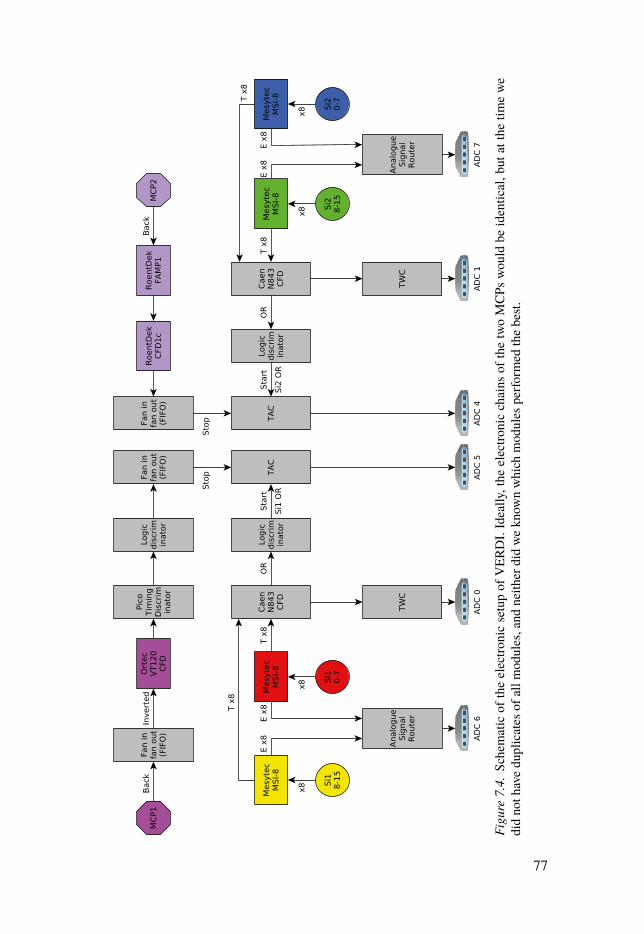
Figu

re7.

4.Sc

hem

atic

ofth

eel

ectro

nic

setu

pof

VER

DI.

Idea

lly,t

heel

ectro

nic

chai

nsof

the

two

MCP

swou

ldbe

iden

tical

,but

atth

etim

ew

edi

dno

thav

edu

plic

ates

ofal

lmod

ules

,and

neith

erdi

dw

ekn

own

whi

chm

odul

espe

rform

edth

ebe

st.

77

fragment, at a distance of 0.5m, by almost 1 cm, i.e, in the same order ofmagnitude as the diameter of the silicon detectors used in the VERDI setup.

To investigate and quantify the kinematical influence of neutron emission, aMonte-Carlo sampling scheme was developed. The simulation was also usedto answer other questions that emerged during the analysis of the experimentaldata, e.g., how the PDT (see section 3.4.2) is best handled.

In order to get realistic mass and energy distribution I used GEF (a GEneraldescription of Fission observables) [16] to generate 1 × 106 spontaneous fissionevents of 252Cf. For each event all necessary properties of both the light andheavy fragments are specified, e.g., mass, kinetic energy and the multiplicityof the neutron emission. Although, GEF manages to reproduce a post-neutronTKE in agreement with measurements of 252Cf(sf ), it does not calculate the fullkinematics of the neutron emission. Unfortunately, this was the information Iwas mainly after.

Therefore, I extracted the pre-neutron state of the fragments and the list ofneutron energies emitted by each fragment in the CoM frame, both generatedby GEF. Subsequently I calculated the neutron emission kinematics relativ-istically, assuming the neutrons were emitted isotropically in the CoM frame.Since GEF also provided γ-emission information the procedure was repeatedfor the γs, even though their kinematical influence on the fragments were min-imal. Since GEF does not list masses but rather the nuclear species (A and Z),I fetched the masses from The Ame2012 atomic mass evaluation [94, 95].

For each event, a realistic PDT was calculated based on the systematic studyof Bohne et al. [96]. The effective fields inside the silicon detectors are wellinside the region I defined by Bohne et al., so the PDT was always calculatedusing eq. 3 in their published article [96].

After neutron emission, one is left with two FPs with an angle betweentheir momenta. Since the VERDI setup positions all silicon detectors facingeach other pair-wise, as well as facing the target, a too large angular deviationfrom 180° might cause one of the fragments to miss its detector, even if theother fragment is properly detected. Next, I will outline how the probabilityof having a coincident event, given that one of the fragment is detected, isestimated.

To aid the reader in the geometrical reasoning a simple sketch has been drawnin fig. 7.5. Assume that fragment one (F1) is detected in silicon detector one(D1). Let the horizontal axis coincide with F1’s trajectory. The position on thedetector surface where F1 hits D1 is uniformly randomised, which determinesD1’s position relative the z-axis. The position of the second detector (D2) isfound by mirroring the vector pointing at D1 from the target centre. Sinceone knows the relative angle, θ, between F1 and the second fragment F2, thetrajectory of F2 only has one degree of freedom, an angle ϕ (not drawn infigure). By uniformly randomising ϕ and evaluating the final position of F2,one can determine whether it hits D2 or not, just by comparing the distancebetween F2 and D2. If it is less than the detector radius, both fragments

78

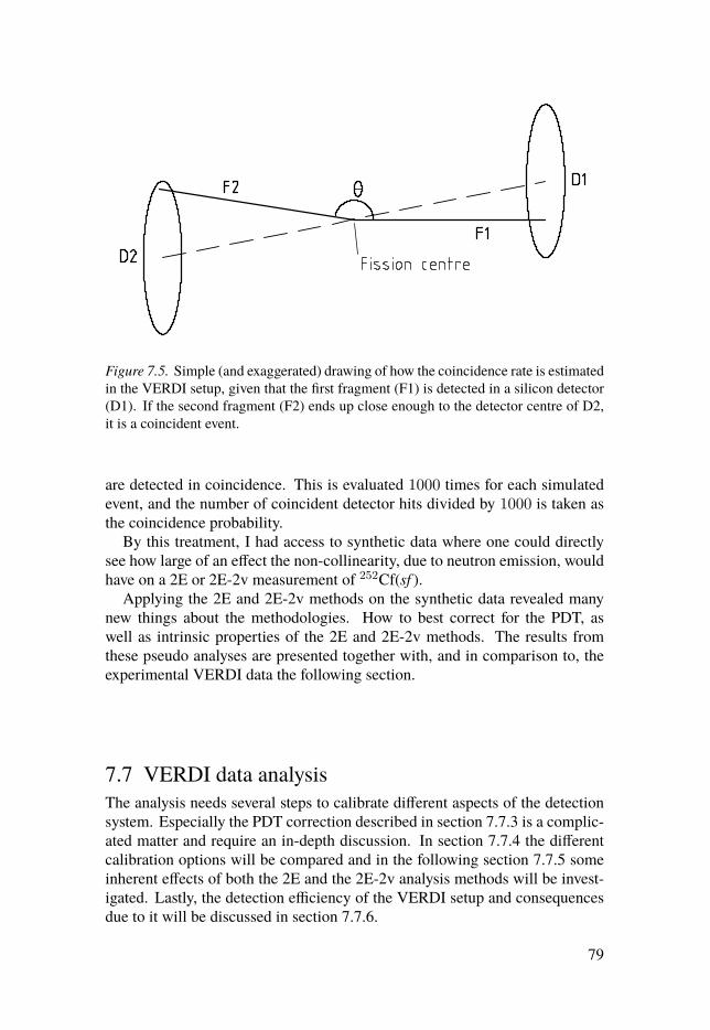
Figure 7.5. Simple (and exaggerated) drawing of how the coincidence rate is estimatedin the VERDI setup, given that the first fragment (F1) is detected in a silicon detector(D1). If the second fragment (F2) ends up close enough to the detector centre of D2,it is a coincident event.

are detected in coincidence. This is evaluated 1000 times for each simulatedevent, and the number of coincident detector hits divided by 1000 is taken asthe coincidence probability.

By this treatment, I had access to synthetic data where one could directlysee how large of an effect the non-collinearity, due to neutron emission, wouldhave on a 2E or 2E-2v measurement of 252Cf(sf ).

Applying the 2E and 2E-2v methods on the synthetic data revealed manynew things about the methodologies. How to best correct for the PDT, aswell as intrinsic properties of the 2E and 2E-2v methods. The results fromthese pseudo analyses are presented together with, and in comparison to, theexperimental VERDI data the following section.

7.7 VERDI data analysisThe analysis needs several steps to calibrate different aspects of the detectionsystem. Especially the PDT correction described in section 7.7.3 is a complic-ated matter and require an in-depth discussion. In section 7.7.4 the differentcalibration options will be compared and in the following section 7.7.5 someinherent effects of both the 2E and the 2E-2v analysis methods will be invest-igated. Lastly, the detection efficiency of the VERDI setup and consequencesdue to it will be discussed in section 7.7.6.

79

Table 7.1. Particle data used for fitting the four parameter schmitt function (eq. 7.19).

Schmitt et al. Iterative Müller et al. ADCM/ amu E/ MeV E/ MeV E/ MeV peak4.0012 6.01 6.01 6.01 α79.92 73.69 73.18 73.33 Heavy79.92 100.57 99.49 99.28 Light126.9 78.45 77.58 77.44 Heavy126.9 107.01 104.59 105.39 Light

7.7.1 Time-of-flight calibrationBy using one of the MCPs as the start signal and the other as the stop signal,the timing resolution was deduced from the resulting distribution width. Thedistribution had a FWHM of 510 ps which corresponds to an individual 360 psFWHM (σ = 150 ps) for each of the MCPs assuming that their respectivetiming resolutions were the same. This is a worse resolution than was foundby Zhang et al., using similar MCPs but with larger channel diameters (25 μminstead of our 13 μm) [33]. However, the estimated resolution includes possiblecontributions from the DAQ system, and the VERDI timing resolution willanyway be dominated by the silicon detector contribution.

Theα-particles coming from the 252Cf sample allow me to calibrate the ToF.The different α-particle energies were not all resolved, rather the estimatedmean energy 6.01MeV was used, based on the relative contributions of theunresolved peaks. In addition to the α-decay from 252Cf, significant amountsof 249Cf, 250Cf, 251Cf and decay products were present.

Since mass, charge and energy were all known for these α-particle it waspossible to correct for the small energy loss in the sample backing. Theselight particles do not suffer from any PDT, thus leaving the ToF to be preciselydetermined. When detecting FPs, this calibration enable VERDI to determinethe time between fission and the main charge collection in the silicon detectors.The PDT, which is suppressing the onset of the charge collection process, mustbe corrected for in these cases.

7.7.2 Energy calibration and PHD correctionsThe energy calibration mainly follows the method outlined by Schmitt et al.[38]. For each of the ADC spectra, coming from single silicon detectors, theα-particle, light FP and heavy FP peaks are localised. Their channel positionsare extracted by gaussian fits in narrow regions around the bin maximums. Thevalues are used to construct an energy calibration.

The α-particle mass and its mean energy are known, while the massesand energies for FPs corresponding to the light and heavy peak, respectively,are taken from Schmitt et al. [38]. This peak data (found in table. 7.1) are

80

corrected for the energy losses due to the sample backing, and then fitted to afour parameter function,

Em = schmitt(x,M) = (a + a′M)x + b + b′M, (7.19)

where Em is the kinetic energy of the detected particle, x the ADC channel, Mthe particle mass. a, a′, b and b′ are the fit parameters. The energy loss, ΔE ,in the target backing is calculated using the free library Range [97] yieldingthe post-neutron energy:

Epost = Em + ΔE(Mpost, Em). (7.20)

Since the 252Cf has diffused into the backing the measured energies of bothsides needs to be corrected based on the average depth of the 252Cf. Themeasured velocities are corrected correspondingly:

�post = �m + Δ� (7.21)

Δ� =

√2Epost

Mpost −√

2EmMpost . (7.22)

The FP energy spectra produced by this calibration agrees fairly well withthe data of Schmitt et al. [38], but overestimates the energy somewhat. How-ever, while it produces a similar 〈TKE〉 as Schmitt et al. it disagrees withlater measurements [98] that measured a significantly lower 〈TKE〉. In orderto remedy this problem several different calibration procedures were tried.The resulting Epost distributions are found in fig. 7.6 and their correspondingparameters values are found in table 7.1.

Among the more successful ones were an iterative procedure. It was basedon a Monte Carlo search in the Schmitt parameter space, trying to reproducewell known quantities like average masses and energies for the light and heavyfragments and ν̄tot. The resulting parameter values, that gave seemingly correctdistributions as well as good average values of TKEpre and TKEpost, are foundin table 7.1 in the ‘iterative’ column.

In the end I settled for using the analytically corrected parameters by Mülleret al. [92], which gave mostly qualitatively similar results as the previouslydescribed iterative method, but required no iterations and are not affected bythe PDT correction discussed in section 7.7.3. That energy calibration alsoimproved the ν̄tot(TKEpre) distribution which is discussed in section 7.7.4.

I also investigated, if one could deviate slightly from the prescription ofSchmitt et al. [38] by using the information of the α-particles in additionto the heavy ion data (and thereby having one more degree of freedom thanthe number of parameters). By also using the α-peak I could apprehend acalibration valid also for lower masses and energies, useful to look for, e.g.,ternary fission. However, some precision in the fission mass region had to besacrificed so it was not used in the main analysis.

81

/ MeVpost

E

40 50 60 70 80 90 100 110 120

Coun

ts / a

.u.

0

1

2

3

4

5

6

7

VERDI (Schmitt)

VERDI (Iterative)

ller)uVERDI (M

Schmitt et al.

k et al.ooG

Figure 7.6. The results of applying different energy calibrations to the VERDI data,compared to the energy distributions of Schmitt et al. [38] and Göök et al. [98].

7.7.3 PDT correctionsThere are many recipes in literature of how one should correct for the PDTin silicon detectors. Studies of the PDT itself have been performed usingaccelerated ions [96, 99] but the results have not been easy to apply to newexperimental setups, so experimentalists have found their own ways of dealingwith this. The true ToF is often determined by the 2E method [93] and due tothe dependence of a previously ‘known’ ν̄ such measurements could arguablybe called 2� assisted 2E. However, as in the case for VERDI, one could useone fairly well known system, i.e. 252Cf(sf ), to calibrate the PDT correction,and after that make a ‘true’ 2E-2v measurement on another system. A similarapproach was used by Müller et al. [92].

7.7.3.1 Former PDT correctionThe PDT correction procedure previously used for the VERDI analysis, ori-ginally suggested by Velkovska and McGrath [99] (hereby referred to as theVelkovska method), prescribes that a linear fit is made, relating the measuredapparent velocity, �m, to the true velocity, �post.

In the case of VERDI, the true velocity was taken as the velocity derivedby the 2E method. However, the linearity is deluding. Since �m ≈ �post it isobvious that the relation can be fairly well described by a linear function. But

82

this relation does not capture the small perturbation introduced by the PDT, atleast not in any other way than a coarse grained average.

Still, this correction is enough to make many of the one dimensional plotsagree quite well with previous measurements and the errors do not show upclearly in the experimental data until you observe correlations in, e.g., twodimensional plots. The, with previous measurements [98], seemingly well-agreeing one-dimensional distributions are depicted in fig. 7.7, while ν̄(Mpre)and ν̄tot(TKEpre) are discussed later together with the results of the othercorrection methods in section 7.7.4.

While the calibration of the energy and the timing can influence each otherin an experimental situation, it is easy to separate them when working withsynthetic data. The energy calibration can cover up problems in the PDTcorrection and vice versa. To properly establish that the linear correction doesnot estimate the PDT well, I made a 2E-2v analysis of the synthetic data, usingthe Velkovska method to correct for the PDT. In fig. 7.8 several plots are shownthat show the effect of correcting the PDT the wrong way.

If one looks carefully, it is clear that the relation between the measured andtrue velocity is not very well represented by a linear function. The ν̄ as afunction of Mpre gets distorted, and the seemingly rather well agreeing exper-imental ν̄(Mpre) (see Ana II in fig. 7.12) is most likely due to a compensationin the energy calibration procedure. One can also directly observe the PDTcorresponding to this correction, which does not reproduce the true PDT andhas a completely different shape. These findings leave only one conclusion,the Velkovska method is ill-suited to correct for the PDT.

7.7.3.2 New iterative PDT parametrisationEven though the Velkovska method turned out to be wrong, one notes thatespecially the Mpre distribution in fig. 7.7 looks really good including a higherpeak-to-valley ratio which can be interpreted as higher resolution. The divisionin eq. 7.14 will, to a large part, cancel systematic errors and that makes theMpre distribution more resilient to small disturbances, e.g., erroneous PDTcorrections. The PDT calculated by the 2E method was therefore parametrisedas a function Mpre and Epre calculated with the 2E-2v method, believing themto be more trustworthy. It would be a more natural choice to parametrise usingMpost and Epost, since those variables actually describe the particle hitting thesilicon detector, but Mpost is expected to have larger uncertainties than Mpre.

For most 1 amu mass intervals the trend was very clear; the PDT as afunction of Epre was a linear function. Fitting linear functions to this data andthen plotting the slope and intercept as functions of Mpre revealed that they toobehaved linearly. These linear behaviours are depicted in fig. 7.9. Thus, onegets a similar parametrisation for the PDT as one already have for the PHD(eq. 7.19):

83

/ amupre

M

80 100 120 140 160 180

Yie

ld /

%

0

1

2

3

4

5

6

7

8

/ amupost

M

80 100 120 140 160 180

Yie

ld /

%

0

1

2

3

4

5

6

7

8

/ amupre

E

50 60 70 80 90 100 110 120 130

Yie

ld /

%

0

1

2

3

4

5

6

7

8

/ amupost

E

50 60 70 80 90 100 110 120 130

Yie

ld /

%

0

1

2

3

4

5

6

7

8

VERDI

k et al.ooG

Figure 7.7. Even though the Velkovska method [99] could be shown (fig. 7.8) tobe incorrect, many distributions were still in good agreement with the previous onesmeasured by Göök et al. [98].

/ cmV

0.03 0.04 0.05

V /

c

0.03

0.04

0.05Synthetic data

Linear fit

/ amupre

M

80 90 100 110 120 130 140 150 160 170

ν

1−

0

1

2

3

4

5

6 Synthetic data

2E2v (Velkovska)

/ amupost

M

80 90 100 110 120 130 140 150 160 170

PD

T /

ns

0

0.5

1

1.5

2

Synthetic data

2E2v (Velkovska)

/ MeVpost

E

50 60 70 80 90 100 110 120

PD

T /

ns

1−

0.5−

0

0.5

1

1.5

2

Synthetic data

2E2v (Velkovska)

Figure 7.8. The Velkovska method fails to reproduce the synthetic data, and the linearrelationship the method is based on is not observed.

84

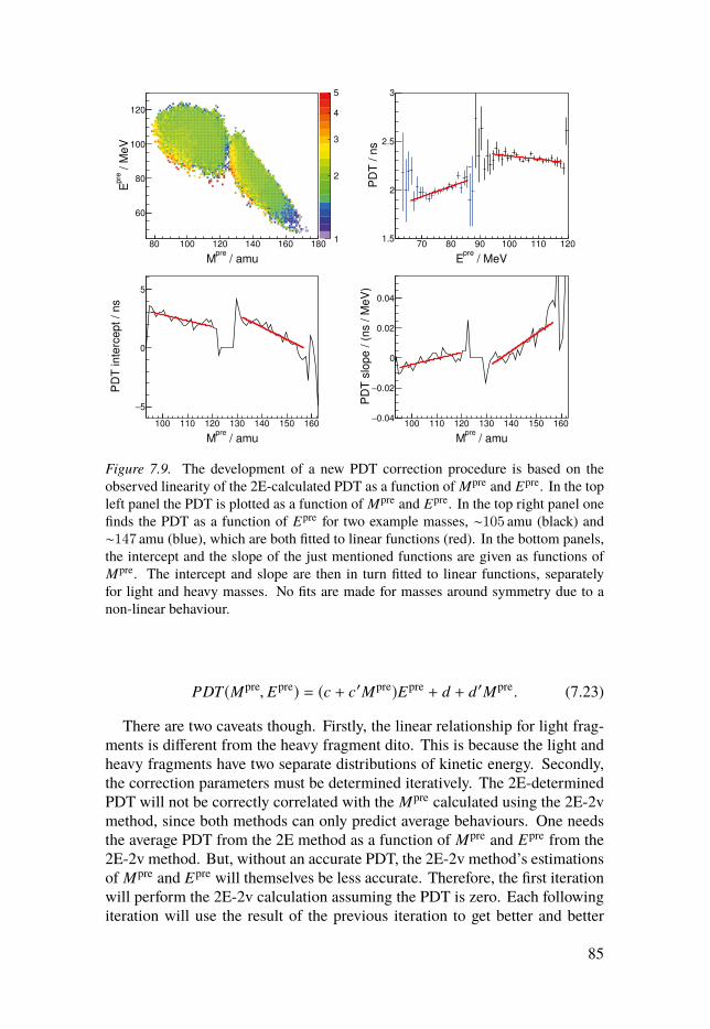
1

2

3

4

5

/ amupre

M

80 100 120 140 160 180

/ M

eV

pre

E

60

80

100

120

/ MeVpre

E

70 80 90 100 110 120

PD

T / n

s

1.5

2

2.5

3

/ amupre

M

100 110 120 130 140 150 160

PD

T inte

rcept / ns

5−

0

5

/ amupre

M

100 110 120 130 140 150 160

PD

T s

lope / (

ns / M

eV

)

0.04−

0.02−

0

0.02

0.04

Figure 7.9. The development of a new PDT correction procedure is based on theobserved linearity of the 2E-calculated PDT as a function of Mpre and Epre. In the topleft panel the PDT is plotted as a function of Mpre and Epre. In the top right panel onefinds the PDT as a function of Epre for two example masses, ∼105 amu (black) and∼147 amu (blue), which are both fitted to linear functions (red). In the bottom panels,the intercept and the slope of the just mentioned functions are given as functions ofMpre. The intercept and slope are then in turn fitted to linear functions, separatelyfor light and heavy masses. No fits are made for masses around symmetry due to anon-linear behaviour.

PDT(Mpre, Epre) = (c + c′Mpre)Epre + d + d ′Mpre. (7.23)

There are two caveats though. Firstly, the linear relationship for light frag-ments is different from the heavy fragment dito. This is because the light andheavy fragments have two separate distributions of kinetic energy. Secondly,the correction parameters must be determined iteratively. The 2E-determinedPDT will not be correctly correlated with the Mpre calculated using the 2E-2vmethod, since both methods can only predict average behaviours. One needsthe average PDT from the 2E method as a function of Mpre and Epre from the2E-2v method. But, without an accurate PDT, the 2E-2v method’s estimationsof Mpre and Epre will themselves be less accurate. Therefore, the first iterationwill perform the 2E-2v calculation assuming the PDT is zero. Each followingiteration will use the result of the previous iteration to get better and better

85

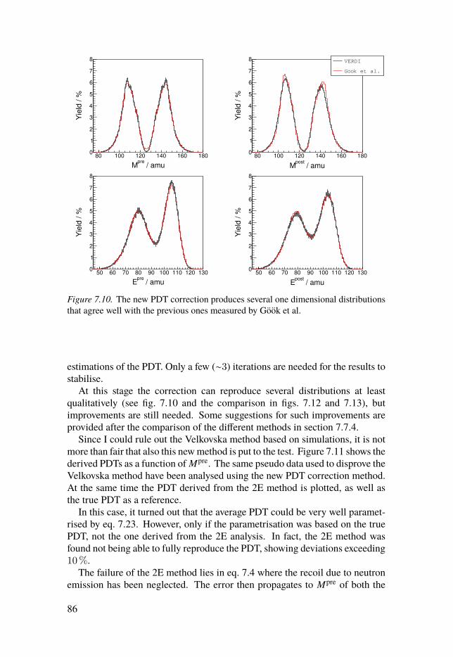
/ amupre

M

80 100 120 140 160 180

Yie

ld / %

0

1

2

3

4

5

6

7

8

/ amupost

M

80 100 120 140 160 180

Yie

ld / %

0

1

2

3

4

5

6

7

8

/ amupre

E

50 60 70 80 90 100 110 120 130

Yie

ld / %

0

1

2

3

4

5

6

7

8

/ amupost

E

50 60 70 80 90 100 110 120 130

Yie

ld / %

0

1

2

3

4

5

6

7

8

VERDI

k et al.ooG

Figure 7.10. The new PDT correction produces several one dimensional distributionsthat agree well with the previous ones measured by Göök et al.

estimations of the PDT. Only a few (∼3) iterations are needed for the results tostabilise.

At this stage the correction can reproduce several distributions at leastqualitatively (see fig. 7.10 and the comparison in figs. 7.12 and 7.13), butimprovements are still needed. Some suggestions for such improvements areprovided after the comparison of the different methods in section 7.7.4.

Since I could rule out the Velkovska method based on simulations, it is notmore than fair that also this new method is put to the test. Figure 7.11 shows thederived PDTs as a function of Mpre. The same pseudo data used to disprove theVelkovska method have been analysed using the new PDT correction method.At the same time the PDT derived from the 2E method is plotted, as well asthe true PDT as a reference.

In this case, it turned out that the average PDT could be very well paramet-rised by eq. 7.23. However, only if the parametrisation was based on the truePDT, not the one derived from the 2E analysis. In fact, the 2E method wasfound not being able to fully reproduce the PDT, showing deviations exceeding10%.

The failure of the 2E method lies in eq. 7.4 where the recoil due to neutronemission has been neglected. The error then propagates to Mpre of both the

86

/ amupre

M

90 100 110 120 130 140 150 160

PD

T / n

s

0

0.2

0.4

0.6

0.8

1

1.2

1.4

1.6

1.8

2

Synthetic data

2E

2E2v (ideal PDT)

2E2v (2E based PDT)

Figure 7.11. The new iterative PDT correction is tested in two ways. One curve showsthe derived PDT when it tries to parametrise the true PDT from the synthetic data.Another curve shows the PDT when the parametrisation is based on the 2E calculatedPDT. The true PDT and the 2E PDT is also shown as references.

fragments through eq. 7.5. The inability to determine the correct ToF, showsthat the 2E-deduced correlation between Mpost and Epost is not correct.

7.7.3.3 Another option?Another very simple correction has been suggested by Brinkmann et al. whichutilises the target backing in a clever way [100]. Small intervals around theheavy and light fragment peaks in the energy spectrum were used in order toknow the mass approximately. Due to the energy loss on the backing sideBrinkmann et al. could calculate how the PDT changed with energy for thepeak masses. The observed PDT behaviour was then extrapolated to the wholedataset.

Unfortunately this is difficult to do for the VERDI setup since much of the252Cf have diffused into the nickel backing of the currently used target. Witha new target the position of the 252Cf would be well defined and this methodcould be attempted.

87

7.7.4 Comparison of calibration methodsWhile it is fairly easy to reproduce one dimensional distributions with sev-eral different calibration methods and parameter sets, the differences show upmore clearly when observing the important variable ν̄ as a function of otherobservables. Especially the correlation between ν̄tot and TKEpre is sensitive toboth the PHD and the PDT correction in use. In figs. 7.12 and 7.13 I show theresults from three different analyses which are defined by the different choicesof PHD and PDT corrections:

Ana I Using the ‘iterative’ Schmitt parameters (see table 7.1) for the PHDcorrection, and the Velkovska method for the PDT correction.

Ana II Using the Schmitt parameters from Müller et al. (table 7.1) for thePHD correction, and the Velkovska method for the PDT correction.

Ana III Using the Schmitt parameters from Müller et al. (table 7.1) for thePHD correction, and the new iterative PDT correction method.

Running the analysis with the set of parameters from Müller et al. alsocorrected an erroneous behaviour when observing ν̄tot as a function of TKEpre.A high TKEpre implies a low TXE. Therefore, one expects a lower ν̄tot forfission events with high TKEpre, since the neutron boil-off only stops whenthere is no excitation energy left to pay for the neutron separation energy with.The negative inverse of the slope therefore relates to the average needed energyneeded to emit a neutron. The kinetic energies of the fragments do not changemuch on average during the neutron emission, so a very similar correlation isexpected for ν̄tot(TKEpost).

When several different correction methods show similar mass and energydistributions ν̄tot(TKEpre) can often tell which ones make sense to use. Amethod not reproducing a reasonable trend in ν̄tot is unacceptable and evenunphysical. In fig. 7.13 one sees one such an example, where the analysis AnaI gives a positive slope for ν̄tot(TKEpre) even though the ν̄(Mpre) in fig. 7.12looks very promising. The slope when Ana II is used (also in fig. 7.13) stilldeviates significantly from the expected value of about −1

12.6 MeV−1 [98], butit is at least negative.

We see improvements going from Ana I to Ana II due to the improvedSchmitt parameter values used in the energy calibration that describes thePHD better. Going from Ana II to Ana III one sees similar performanceswhen looking at ν̄(Mpre) in fig. 7.12, but Ana III gives slightly better slopes infig. 7.13. The slope for Ana III corresponds to 12.7MeV per neutron in theTKEpost case, but 23.5MeV per neutron for the TKEpre case. For Ana II thesenumbers instead become 15.4MeV and 39MeV per neutron, for TKEpost andTKEpre respectively.

It might still require some refinements, but the new iterative PDT correctionmethod is currently the most promising for VERDI at the moment. Compar-ing the analysis options once again in fig. 7.14, one sees how the new PDT

88

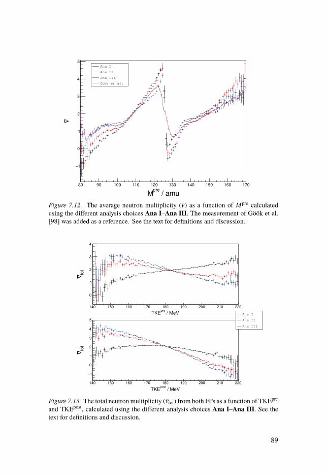
/ amupre

M

80 90 100 110 120 130 140 150 160 170

ν

1−

0

1

2

3

4

5Ana I

Ana II

Ana III

k et al.ooG

Figure 7.12. The average neutron multiplicity (ν̄) as a function of Mpre calculatedusing the different analysis choices Ana I–Ana III. The measurement of Göök et al.[98] was added as a reference. See the text for definitions and discussion.

/ MeVpre

TKE

140 150 160 170 180 190 200 210 220

tot

ν

0

1

2

3

4

/ MeVpost

TKE

140 150 160 170 180 190 200 210 220

tot

ν

1−

0

1

2

3

4

5

Ana I

Ana II

Ana III

Figure 7.13. The total neutron multiplicity (ν̄tot) from both FPs as a function of TKEpre

and TKEpost, calculated using the different analysis choices Ana I–Ana III. See thetext for definitions and discussion.

89

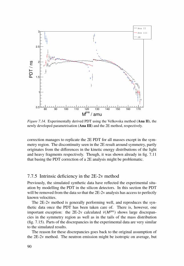
/ amupre

M

80 90 100 110 120 130 140 150 160 170

PD

T / n

s

0.5

1

1.5

2

2.5

3

Ana II

Ana III

2E

Figure 7.14. Experimentally derived PDT using the Velkovska method (Ana II), thenewly developed parametrisation (Ana III) and the 2E method, respectively.

correction manages to replicate the 2E PDT for all masses except in the sym-metry region. The discontinuity seen in the 2E result around symmetry, partlyoriginates from the differences in the kinetic energy distributions of the lightand heavy fragments respectively. Though, it was shown already in fig. 7.11that basing the PDT correction of a 2E analysis might be problematic.

7.7.5 Intrinsic deficiency in the 2E-2v methodPreviously, the simulated synthetic data have reflected the experimental situ-ation by modelling the PDT in the silicon detectors. In this section the PDTwill be removed from the data so that the 2E-2v analysis has access to perfectlyknown velocities.

The 2E-2v method is generally performing well, and reproduces the syn-thetic data once the PDT has been taken care of. There is, however, oneimportant exception: the 2E-2v calculated ν̄(Mpre) shows large discrepan-cies in the symmetry region as well as in the tails of the mass distribution(fig. 7.15). Parts of the discrepancies in the experimental data are very similarto the simulated results.

The reason for these discrepancies goes back to the original assumption ofthe 2E-2v method. The neutron emission might be isotropic on average, but

90

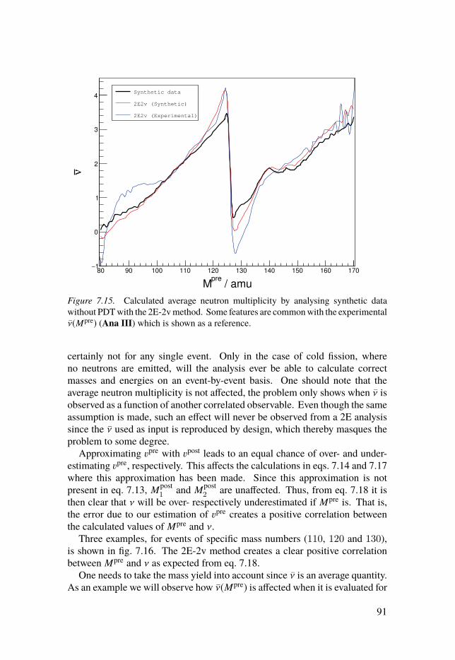
/ amupre

M

80 90 100 110 120 130 140 150 160 170

ν

1−

0

1

2

3

4Synthetic data

2E2v (Synthetic)

2E2v (Experimental)

Figure 7.15. Calculated average neutron multiplicity by analysing synthetic datawithout PDT with the 2E-2v method. Some features are common with the experimentalν̄(Mpre) (Ana III) which is shown as a reference.

certainly not for any single event. Only in the case of cold fission, whereno neutrons are emitted, will the analysis ever be able to calculate correctmasses and energies on an event-by-event basis. One should note that theaverage neutron multiplicity is not affected, the problem only shows when ν̄ isobserved as a function of another correlated observable. Even though the sameassumption is made, such an effect will never be observed from a 2E analysissince the ν̄ used as input is reproduced by design, which thereby masques theproblem to some degree.

Approximating �pre with �post leads to an equal chance of over- and under-estimating �pre, respectively. This affects the calculations in eqs. 7.14 and 7.17where this approximation has been made. Since this approximation is notpresent in eq. 7.13, Mpost

1 and Mpost2 are unaffected. Thus, from eq. 7.18 it is

then clear that ν will be over- respectively underestimated if Mpre is. That is,the error due to our estimation of �pre creates a positive correlation betweenthe calculated values of Mpre and ν.

Three examples, for events of specific mass numbers (110, 120 and 130),is shown in fig. 7.16. The 2E-2v method creates a clear positive correlationbetween Mpre and ν as expected from eq. 7.18.

One needs to take the mass yield into account since ν̄ is an average quantity.As an example we will observe how ν̄(Mpre) is affected when it is evaluated for

91

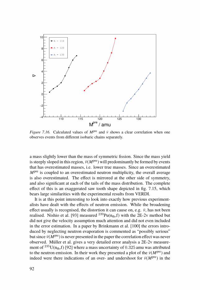
/ amupre

M

110 115 120 125 130

ν

4−

2−

0

2

4

6

8

10A = 110

A = 120

A = 130

Figure 7.16. Calculated values of Mpre and ν̄ shows a clear correlation when oneobserves events from different isobaric chains separately.

a mass slightly lower than the mass of symmetric fission. Since the mass yieldis steeply sloped in this region, ν̄(Mpre)will predominantly be formed by eventsthat has overestimated masses, i.e. lower true masses. Since an overestimatedMpre is coupled to an overestimated neutron multiplicity, the overall averageis also overestimated. The effect is mirrored at the other side of symmetry,and also significant at each of the tails of the mass distribution. The completeeffect of this is an exaggerated saw tooth shape depicted in fig. 7.15, whichbears large similarities with the experimental results from VERDI.

It is at this point interesting to look into exactly how previous experiment-alists have dealt with the effects of neutron emission. While the broadeningeffect usually is recognised, the distortion it can cause on, e.g. ν̄, has not beenrealised. Nishio et al. [93] measured 239Pu(nth,f) with the 2E-2v method butdid not give the velocity assumption much attention and did not even includedin the error estimation. In a paper by Brinkmann et al. [100] the errors intro-duced by neglecting neutron evaporation is commented as “possibly serious”but since ν̄(Mpre) is never presented in the paper the correlation effect was neverobserved. Müller et al. gives a very detailed error analysis a 2E-2v measure-ment of 235U(nth,f) [92] where a mass uncertainty of 0.325 amu was attributedto the neutron emission. In their work they presented a plot of the ν̄(Mpre) andindeed were there indications of an over- and undershoot for ν̄(Mpre) in the

92

symmetry region. However, it was interpreted as a “better mass resolution”(FIG. 11 and 12 in ref. [92]). Since they never mentioned any correction forthe found correlation problem, I must assume that their results were affectedby it, and need to be corrected.

I will now derive a correction procedure by deconvoluting the resultingν̄(Mpre) from the 2E-2v method. It is a simple correction that can be appliedalso to previously measured data and it does not rely on any input data except themeasured (uncorrected) pre-neutron mass distribution and neutron multiplicity.

The algorithm works with binned data, preferably with much smaller binsthan the experimental resolution. In my implementation, a bin width of 0.1 amuwas used. First I construct a response matrix R relating the actual pre-neutronmass Mc with the obtained measured pre-neutron mass Mm such that

Mmi =

∑j

Ri jMcj . (7.24)

The neutron emission appear as a broadening of the mass resolution whichcan be kinematically estimated using the preliminary ν̄(Mpre). In the caseof 252Cf(sf ) the standard deviation due to neutron emission was on average0.8 amu. The mass dependant estimates are depicted in fig. 7.17, where onesees how the broadening follows the shape of the total neutron multiplicitysince both velocities affect Mpre (eq. 7.14). The response from each true massMc was modelled by a gaussian centred on Mc with a mass dependent widthaccording to fig. 7.17. The mass spectrum is taken into account by weightingeach matrix element Ri j with the yield Y (Mc

j ).To express the inverse relationship,

Mcj =

∑i

Ri jMmi . (7.25)

it was assumed that the transpose of R could approximate R−1, even though Ris not necessarily strictly orthogonal.

I find the correction formula by expressing the actual ν̄c,

ν̄cj =1

mn

(Mc

j − Mpostj

)=

1

mn

∑i

Ri j

(Mm

i −(Mpost

i + ΔMi j

)), (7.26)

where I have used eq. 7.25 to rewrite Mcj , and ΔMi j is just the distance between

the bins i and j in mass units. Since ν̄mi = (Mmi −Mpost

i )/mn, this can be written

ν̄cj =∑i

Ri j

(ν̄mi − ΔMi j

mn

). (7.27)

This rather crude correction method reproduces the true ν̄(Mpre) well. Fig-ure 7.18 shows the resulting corrected ν̄(Mpre). The total average neutron

93

/ amupre

M

80 90 100 110 120 130 140 150 160

/ a

mu

σ

0

0.1

0.2

0.3

0.4

0.5

0.6

0.7

0.8

0.9

1

/ a

mu

tot

ν

0

1

2

3

4

5

6

7

8

σCf 252

σU 235

totνCf 252

totνU 235

Figure 7.17. Standard deviations of the mass broadening due to neutron emission,for 252Cf(sf ) and 235U(n,f), respectively. The total average neutron multiplicity ν̄tot isplotted as a reference.

multiplicity is conserved, but a smearing effect is present, leaving some struc-tures in the synthetic ν̄(Mpre) unresolved.

Regarding the previously mentioned results from Müller et al., the lowerneutron multiplicity of 235U(nth,f) compared to 252Cf(sf ), makes the exag-geration of ν̄(Mpre) less severe, but I observed the same trend of over- andundershoots by running our simulation also for the 235U(nth,f) case (fig. 7.19).The synthetic ν̄ generated by the gef code shows much more structure than onesees in experimental data, but this makes it an even better test to determine howmuch of the structure in the synthetic data the correction method reproduces.

In both figs. 7.18 and 7.19 the mass yield was added as a reference. Onecan easily see how the correction is the largest where the mass yield changesthe most between neighbouring masses.

7.7.6 Detection efficiencyWithout neutron emission, the detection of one FP would also result in adetection of the complementary FP, as long as one is dealing with spontaneousfission. For the overwhelming majority of the 252Cf(sf ) events one or moreneutrons will be emitted, and the higher the multiplicity the larger risk it is that

94

/ amupre

M

80 90 100 110 120 130 140 150 160 170

ν

0.5−

0

0.5

1

1.5

2

2.5

3

3.5

4

4.5

Mass y

ield

/ %

0

1

2

3

4

5

6

7Truth

2E-2v

2E-2v Corrected

Mass yield

Figure 7.18. The corrected ν̄(Mpre) from 252Cf(sf ) shows signs of smearing, butreproduces the synthetic data well apart from that. The ‘true’ ν̄(Mpre), the uncorrectedν̄(Mpre) and the mass yield are shown as references.

/ amupre

M

80 90 100 110 120 130 140 150

ν

0

0.5

1

1.5

2

2.5

3

Mass y

ield

/ %

0

1

2

3

4

5

6

7

8Truth

2E-2v

2E-2v Corrected

Mass yield

Figure 7.19. The correction method behaves the same way applied to ν̄(Mpre) from235U(nth,f) as when it is applied to ν̄(Mpre) from 252Cf(sf ). The ‘true’ ν̄(Mpre), theuncorrected ν̄(Mpre) and the mass yield are shown as references.

95

/ MeVpre

TKE

150 160 170 180 190 200 210 220

Coin

cid

ence p

robabili

ty

0

0.1

0.2

0.3

0.4

0.5

0.6

0.7

0.8

0.9

1

Figure 7.20. The simulation shows that the detection efficiency is strongly dependenton TKEpre

not both FPs will be detected in coincidence. The effect the detector efficiencymight have on the observables was investigated by calculating the coincidenceprobability for each event as outlined in section 7.6.

I explained previously in section 7.7.4 how the average total neutron mul-tiplicity is inversely proportional to the TKEpre. Not surprisingly, one sees infig. 7.20 a much lower detection efficiency, around 40%, for events with lowTKEpre while it reaches more or less 100% for high TKEpre.

This bias for events with low neutron multiplicity will distort the shape ofsome distributions which is demonstrated in fig. 7.21. The mass distributionsare not greatly affected, since each mass can be emitted with an energy sampledfrom a broad energy distribution. Although, some of the structure due to theproton-neutron ratio start to wash out.

The energy distributions however, shift toward higher energies since highenergy events are favoured. It is therefore important that the energy calibrationis performed without a coincidence condition, or the wrong peak positionswould be obtained.

Even though the mass distributions are less affected, the ν̄(Mpre)will be gen-erally slightly underestimated under coincidence conditions, especially wherethe neutron multiplicity is the highest (see fig. 7.22).

The experimental data collected with VERDI exhibits an instrumental asym-metry, which is not explained by the efficiency due to neutron emission. It only

96

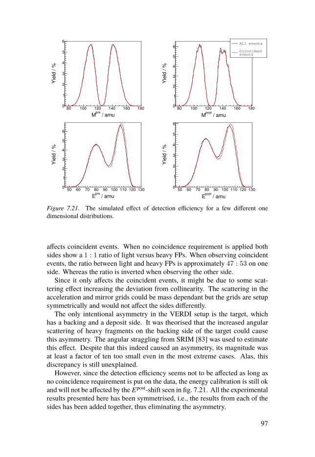
/ amupre

M

80 100 120 140 160 180

Yie

ld / %

0

1

2

3

4

5

6

/ amupost

M

80 100 120 140 160 180

Yie

ld / %

0

1

2

3

4

5

6

/ amupre

E

50 60 70 80 90 100 110 120 130

Yie

ld / %

0

1

2

3

4

5

6

/ amupost

E

50 60 70 80 90 100 110 120 130

Yie

ld / %

0

1

2

3

4

5

6

All events

eventsCoincident

Figure 7.21. The simulated effect of detection efficiency for a few different onedimensional distributions.

affects coincident events. When no coincidence requirement is applied bothsides show a 1 : 1 ratio of light versus heavy FPs. When observing coincidentevents, the ratio between light and heavy FPs is approximately 47 : 53 on oneside. Whereas the ratio is inverted when observing the other side.

Since it only affects the coincident events, it might be due to some scat-tering effect increasing the deviation from collinearity. The scattering in theacceleration and mirror grids could be mass dependant but the grids are setupsymmetrically and would not affect the sides differently.

The only intentional asymmetry in the VERDI setup is the target, whichhas a backing and a deposit side. It was theorised that the increased angularscattering of heavy fragments on the backing side of the target could causethis asymmetry. The angular straggling from SRIM [83] was used to estimatethis effect. Despite that this indeed caused an asymmetry, its magnitude wasat least a factor of ten too small even in the most extreme cases. Alas, thisdiscrepancy is still unexplained.

However, since the detection efficiency seems not to be affected as long asno coincidence requirement is put on the data, the energy calibration is still okand will not be affected by the Epost-shift seen in fig. 7.21. All the experimentalresults presented here has been symmetrised, i.e., the results from each of thesides has been added together, thus eliminating the asymmetry.

97

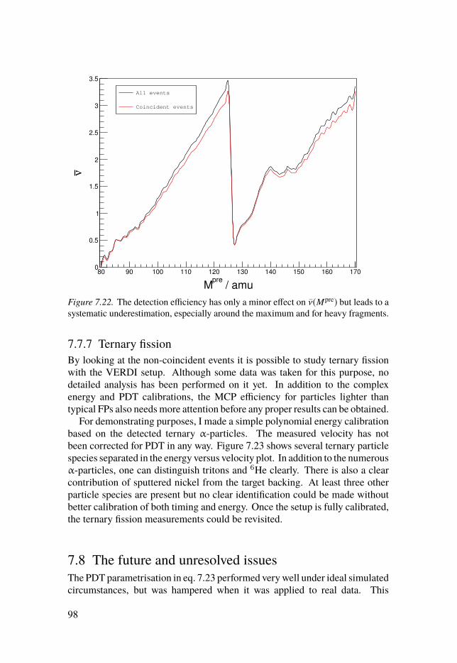
/ amupre

M

80 90 100 110 120 130 140 150 160 170

ν

0

0.5

1

1.5

2

2.5

3

3.5

All events

Coincident events

Figure 7.22. The detection efficiency has only a minor effect on ν̄(Mpre) but leads to asystematic underestimation, especially around the maximum and for heavy fragments.

7.7.7 Ternary fissionBy looking at the non-coincident events it is possible to study ternary fissionwith the VERDI setup. Although some data was taken for this purpose, nodetailed analysis has been performed on it yet. In addition to the complexenergy and PDT calibrations, the MCP efficiency for particles lighter thantypical FPs also needs more attention before any proper results can be obtained.

For demonstrating purposes, I made a simple polynomial energy calibrationbased on the detected ternary α-particles. The measured velocity has notbeen corrected for PDT in any way. Figure 7.23 shows several ternary particlespecies separated in the energy versus velocity plot. In addition to the numerousα-particles, one can distinguish tritons and 6He clearly. There is also a clearcontribution of sputtered nickel from the target backing. At least three otherparticle species are present but no clear identification could be made withoutbetter calibration of both timing and energy. Once the setup is fully calibrated,the ternary fission measurements could be revisited.

7.8 The future and unresolved issuesThe PDT parametrisation in eq. 7.23 performed very well under ideal simulatedcircumstances, but was hampered when it was applied to real data. This

98

V / (cm/ns)

0.6 0.8 1 1.2 1.4 1.6 1.8 2 2.2 2.4 2.6 2.8

E / M

eV

5

10

15

20

25

3H

4He

58Ni 6He

Figure 7.23. Ternary particles detected by VERDI. The energy calibration is onlyapproximate. The solid lines represent the energy calculated using the measuredvelocities and the respective particle masses.

happened because the PDT from the 2E method was used. VERDI is thereforein need of either an independent characterisation of all its silicon detectors, ora working theoretical model of the PDT mass and energy dependence.

One could, for example, take the expression given by Bohne et al. andcombine most of the constants:

PDT = C1Z̄2

Mpost(d − x) exp(−C2

Epost

Mpost

), (7.28)

where Z̄ is the effective charge, d the depletion depth and x the median depthof the created electron-hole pairs. C1 and C2 are the two remaining parametersthat could be fit to the VERDI detector characteristics. The parametrisationof Bohne et al. has previously turned out to be difficult to adapt to new sets ofsilicon detectors [100], but treating C1 and C2 as free parameters might remedythis if the functional form is sound. A first attempt to do this for VERDI wasperformed, but was unsuccessful as it was found that every single detectorwould need different parameters and the lack of reference PDT made it difficultto determine the parameters. The model also showed a heavy dependency ofhow the average charge was calculated, indicating that the expression mightnot be very general. It seems a detailed characterisation of the detectors willbe needed for this to work.

99

A longer flight path would effectively decrease the importance of the PDTcorrection, but also further reduce the detection efficiency, which is alreadycausing trouble since it was shown to be strongly dependent on neutron emis-sion (fig. 7.20). Increasing the size of the silicon detectors could remedy thisbut only if they keep their good timing properties. If silicon strip detectorscould provide good enough timing resolution, it would be an interesting choicealso due to the position sensitivity. The detection efficiency will see even largerchallenges once VERDI measures neutron-induced fission, since the neutronmomentum transfer from the primary neutron will affect the angle between thefragments in an energy dependent manner.

Overall the VERDI project is making progress, even though there are sev-eral improvements needed, especially for the PDT correction procedure. Therecent scrutiny of the analysis procedure identified a flaw, overlooked by manyprevious experimentalists. It can be corrected by a simple deconvolution pro-cedure, but with some smearing as a side effect. Considering that, in additionto VERDI, several 2E-2v projects [101–103] are under development aroundthe word, it is important to show that it is possible to obtain correct independentdata. Next, one needs to determine how much and in what way this limits theobtainable resolution of these upcoming experiments.

When the PDT can be well estimated, the detection efficiency has beenimproved, and the intrinsic problems of the 2E-2v method have been overcome,the next step for VERDI is to confirm all calibrations and corrections againsta new fissioning system. Thermal neutron-induced fission of 235U is alsoa well known system and would serve as a cross-check of the calibrationsachieved with 252Cf(sf ). Once a successful measurement of 235U(nth,f) isachieved, many systems, including neutron-induced fission at higher energies,are waiting.

100

8. Simulated ion stopping at IGISOL

Finland, Finland, Finland.The country where I want to be,pony trekking or camping, or justwatching TV.

— Michael Palin

As mentioned in section 4.3, yield measurements using the IGISOL methodrelies on the measured isotope yield to be compared to the yield of anotherisotope. That isotope must exhibit the same stopping, extraction, and transportefficiency through out the whole system, from the fission moment until thelast capture and detection in the Penning trap. In order to compare yields ofnon-neighbouring isotopes there must be a connection through several relativemeasurements.

Approximate efficiencies are known, partly based on the large experiencegathered at IGISOL, but systematic studies of them are lacking. Knowingthem better could allow for a better understanding of the experiments, andpossibly identification of problems or improvements to the method. Onepossible improvement could be optimising the efficiencies in order to studymore low-yield FPs.

At IGISOL experiments are conducted both for measuring fission yields[104] but also for the production and study of exotic nuclei. Most previousmeasurements at IGISOL up until now, has been using proton-induced fis-sion [45]. Neutron-induced fission changes the yield significantly, especiallyfor neutron-rich FPs. Previous experiments, using neutron-induced fission,reported a shift of the average atomic charge value by 0.88, compared tothe proton-induced case [105]. In fig. 8.1 it is demonstrated how the pre-dicted neutron-induced yields for different tin isotopes compares to the proton-induced yields. These tin nuclei in particular are important to understandthe r-process [106], a mechanism to create nuclei heavier than iron throughcosmological nucleosynthesis.

For the studies of the proton-induced case, which were published in 2015[107], I wrote the simulation software and assisted the analysis. When itcomes to the neutron-induced studies, I developed the simulation software andperformed the analysis.

101

Figure 8.1. Estimates of the yields of different tin isotopes from neutron- and proton-induced fission of 238U. The yields were calculated using GEF [16] for 12MeV neutronand 25MeV protons, respectively.

8.1 Ion guide for proton-induced fission8.1.1 Experimental setupThe experimental setup for this experiment is rather simple and is depicted infig. 8.2. The proton beam hits a natural uranium target at a 7° angle. Only a fewper cent of the FPs will escape the 15mg/cm2 thick target into the 200Torrhelium stopping gas filling the chamber. In order to shield the rest of the ionguide from the plasma induced by the proton beam a thin (1mg/cm2) nickelfoil is separating the target from the rest of the chamber volume. Only the FPsthat pass through the nickel foil have a chance to be transported by the gas andbe accelerated into the rest of the IGISOL setup (see section 4.3).

8.1.2 Simulation setupIn the simulation we neglected the beam attenuation inside the target, sinceprotons are deeply penetrative particles. That means that the probability ofhaving a fission event is constant over the whole target volume as long as thebeam is completely illuminating the target. We therefore completely neglectedthe primary particles and started the simulation by creating heavy ions of

102

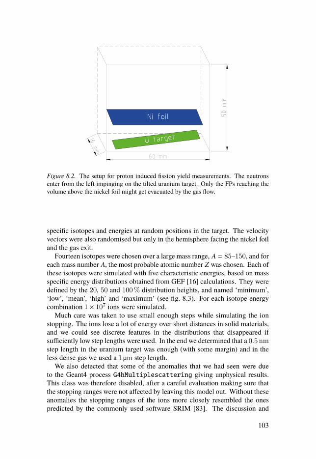
Figure 8.2. The setup for proton induced fission yield measurements. The neutronsenter from the left impinging on the tilted uranium target. Only the FPs reaching thevolume above the nickel foil might get evacuated by the gas flow.

specific isotopes and energies at random positions in the target. The velocityvectors were also randomised but only in the hemisphere facing the nickel foiland the gas exit.

Fourteen isotopes were chosen over a large mass range, A = 85–150, and foreach mass number A, the most probable atomic number Z was chosen. Each ofthese isotopes were simulated with five characteristic energies, based on massspecific energy distributions obtained from GEF [16] calculations. They weredefined by the 20, 50 and 100% distribution heights, and named ‘minimum’,‘low’, ‘mean’, ‘high’ and ‘maximum’ (see fig. 8.3). For each isotope-energycombination 1 × 107 ions were simulated.

Much care was taken to use small enough steps while simulating the ionstopping. The ions lose a lot of energy over short distances in solid materials,and we could see discrete features in the distributions that disappeared ifsufficiently low step lengths were used. In the end we determined that a 0.5 nmstep length in the uranium target was enough (with some margin) and in theless dense gas we used a 1 μm step length.

We also detected that some of the anomalies that we had seen were dueto the Geant4 process G4hMultiplescattering giving unphysical results.This class was therefore disabled, after a careful evaluation making sure thatthe stopping ranges were not affected by leaving this model out. Without theseanomalies the stopping ranges of the ions more closely resembled the onespredicted by the commonly used software SRIM [83]. The discussion and

103

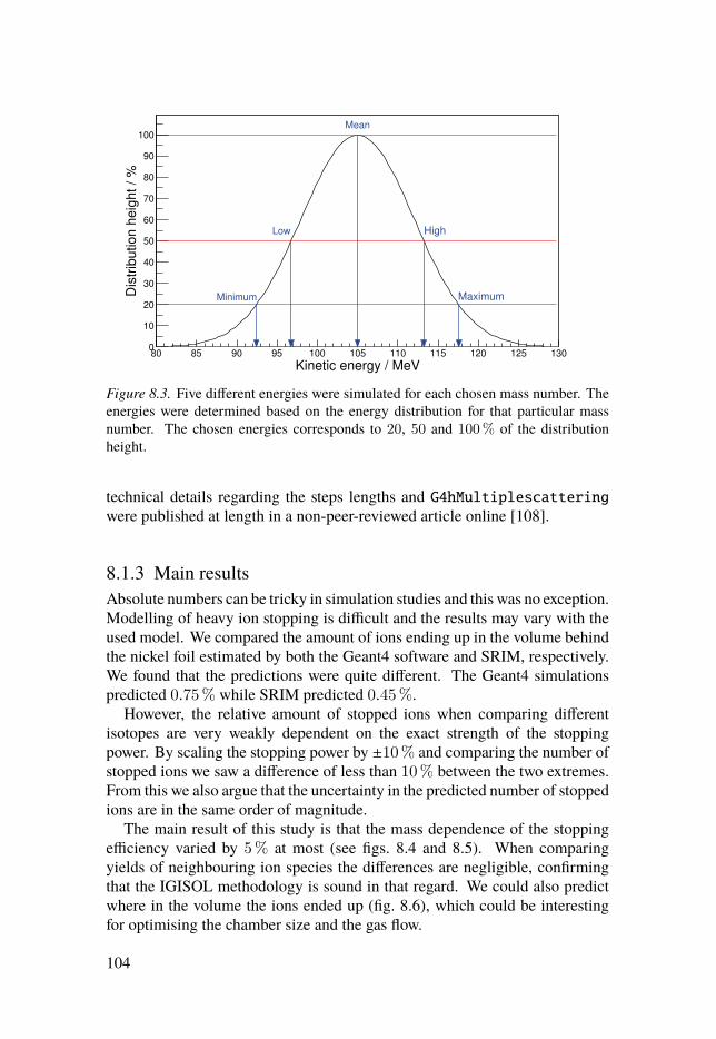
Kinetic energy / MeV80 85 90 95 100 105 110 115 120 125 130

Dis

trib

utio

n h

eig

ht

/ %

0

10

20

30

40

50

60

70

80

90

100

Minimum

Low

Mean

High

Maximum

Figure 8.3. Five different energies were simulated for each chosen mass number. Theenergies were determined based on the energy distribution for that particular massnumber. The chosen energies corresponds to 20, 50 and 100% of the distributionheight.

technical details regarding the steps lengths and G4hMultiplescatteringwere published at length in a non-peer-reviewed article online [108].

8.1.3 Main resultsAbsolute numbers can be tricky in simulation studies and this was no exception.Modelling of heavy ion stopping is difficult and the results may vary with theused model. We compared the amount of ions ending up in the volume behindthe nickel foil estimated by both the Geant4 software and SRIM, respectively.We found that the predictions were quite different. The Geant4 simulationspredicted 0.75% while SRIM predicted 0.45%.

However, the relative amount of stopped ions when comparing differentisotopes are very weakly dependent on the exact strength of the stoppingpower. By scaling the stopping power by ±10% and comparing the number ofstopped ions we saw a difference of less than 10% between the two extremes.From this we also argue that the uncertainty in the predicted number of stoppedions are in the same order of magnitude.

The main result of this study is that the mass dependence of the stoppingefficiency varied by 5% at most (see figs. 8.4 and 8.5). When comparingyields of neighbouring ion species the differences are negligible, confirmingthat the IGISOL methodology is sound in that regard. We could also predictwhere in the volume the ions ended up (fig. 8.6), which could be interestingfor optimising the chamber size and the gas flow.

104

Mass number

90 100 110 120 130 140 150

Sto

pp

ed

io

ns /

%

0.73

0.74

0.75

0.76

0.77

Minimum

Low

Mean

High

Maximum

Figure 8.4. Percent of the simulated ions that stop in the area behind the nickel foil, asa function of mass number. The different curves correspond to the energies defined infig. 8.3.

Kinetic energy / MeV

50 60 70 80 90 100 110

Sto

pp

ed

io

ns /

%

0.73

0.74

0.75

0.76

0.77A85

A90

A95

A100

A105

A110

A115

A120

A125

A130

A135

A140

A145

A150

Figure 8.5. Percent of the simulated ions that stop in the area behind the nickel foil, asa function of initial kinetic energy.

105

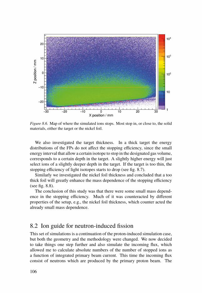
Figure 8.6. Map of where the simulated ions stops. Most stop in, or close to, the solidmaterials, either the target or the nickel foil.

We also investigated the target thickness. In a thick target the energydistributions of the FPs do not affect the stopping efficiency, since the smallenergy interval that allow a certain isotope to stop in the designated gas volume,corresponds to a certain depth in the target. A slightly higher energy will justselect ions of a slightly deeper depth in the target. If the target is too thin, thestopping efficiency of light isotopes starts to drop (see fig. 8.7).

Similarly we investigated the nickel foil thickness and concluded that a toothick foil will greatly enhance the mass dependence of the stopping efficiency(see fig. 8.8).

The conclusion of this study was that there were some small mass depend-ence in the stopping efficiency. Much of it was counteracted by differentproperties of the setup, e.g., the nickel foil thickness, which counter acted thealready small mass dependence.

8.2 Ion guide for neutron-induced fissionThis set of simulations is a continuation of the proton-induced simulation case,but both the geometry and the methodology were changed. We now decidedto take things one step further and also simulate the incoming flux, whichallowed me to calculate absolute numbers of the number of stopped ions asa function of integrated primary beam current. This time the incoming fluxconsist of neutrons which are produced by the primary proton beam. The

106

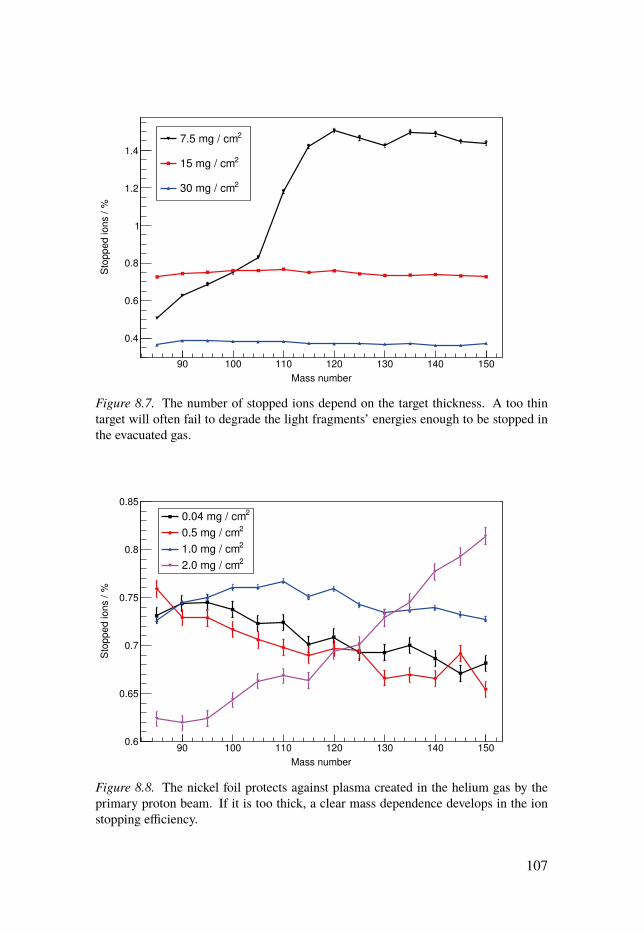
Mass number

90 100 110 120 130 140 150

Sto

pp

ed

io

ns /

%

0.4

0.6

0.8

1

1.2

1.4

27.5 mg / cm

215 mg / cm

230 mg / cm

Figure 8.7. The number of stopped ions depend on the target thickness. A too thintarget will often fail to degrade the light fragments’ energies enough to be stopped inthe evacuated gas.

Mass number

90 100 110 120 130 140 150

Sto

pp

ed

io

ns /

%

0.6

0.65

0.7

0.75

0.8

0.8520.04 mg / cm

20.5 mg / cm21.0 mg / cm22.0 mg / cm

Figure 8.8. The nickel foil protects against plasma created in the helium gas by theprimary proton beam. If it is too thick, a clear mass dependence develops in the ionstopping efficiency.

107

0

2

4

6

8

10

12

14

16

6−10×

Figure 8.9. The neutron flux in n/(cm2 μCs) calculated by MCNPX, on top of aschematic of the ion guide. The flux was only recorded in a cylindrical shell enclosingthe target positions. To the left of the ion guide is the neutron source. The berylliumtarget (grey striped pattern) is cooled by the water (blue wave pattern).

neutron production was simulated separately by A. Solders, while my Geant4software took care of the FP transport simulation.

In December 2016 a yield measurement was performed using this setup forneutron induced fission, which allows me to make some comparison betweensimulation and reality.

8.2.1 The neutron sourceTo produce neutrons, a 30MeV proton beam impinge on a water-cooled beryl-lium target. The neutron production target is thick (5mm) but designed toallow the primary beam to go through and deposit the last of its energy inthe cooling water (pressurised to 7 bar), on the back side of the target. Thisreduces wear on the target since there is less hydrogen build-up in the beryl-lium, but also activates the cooling water, thus requiring a closed circuit. Itwas later decided to add another centimetre of beryllium in order to reduce theactivation. Behind the cooling water, the ion guide with one or several uraniumtargets followed, with only a thin (3mm) aluminium window in between, inorder to make the best use of the neutron flux [46, 109].

108

The neutron converter has been simulated using MCNPX 2.5.0 [110] andthe neutron flux was recorded in a 7mm thick cylindrical shell, enclosing allregions where targets were positioned. The calculated neutron flux integratedover all energies is depicted in fig. 8.9 on top of a schematic of the ionguide. The simulated geometry included the ion guide but not the uraniumtargets inside since the attenuation of the neutron flux in the uranium targets isnegligible. It can easily be shown that the attenuation can be neglected sincethe mass attenuation coefficient is

μm = σNA/MU ≈ 2.5cm2

g, (8.1)

where σ ≈ 1 b is the cross section, NA Avogadro’s number and MU the molarmass of natural uranium. The standard targets are 14mg/cm2 thick leaving uswith an attenuation in the order of 1 × 10−5.

The flux was acquired in 1MeV bins from 1 to 30MeV and exported to textfiles that were later read by the main simulation software.

8.2.2 The ion guideThe chamber where the FPs are produced and collected is called the ion guide.It is gas-filled and the main part of it is cylindrical with a length of about 70mmand a diameter of 60mm. As in the proton-induced case the gas is supposed tostop the ions so that they can be extracted from the ion guide by the helium gasflow. The nominal gas pressure is 200mbar, but in the experiment conductedin December it was increased to 400mbar. A 3D rendering of the standardreference setup [47] is depicted in fig. 8.10.

Three different versions of the setup were implemented and investigated,each depicted as cross-sectional drawings in figs. 8.11a to 8.11c. The defaultsetup mirrors the experimental setup used during measurements at the IGISOLfacility in December 2016. It features two uranium targets close to the neutronproduction, in order to maximise the neutron flux. These targets are 10mm ×50mm with a thickness of 15mg/cm2. There is also an implantation foil inthe back made out of titanium.

The implantation foil makes it possible for us to compare the simulations tothe experiment in December 2016 by analysis the γ-spectrum. This is howeverstill in progress and results are pending. Nevertheless, doing so might providefurther experimental verification of the simulation’s validity.

Another option is to simulate six targets of the same dimension as theprevious mentioned, each fixed on one of the hexagonal sides of the ion guidetarget holder. In this case the titanium foil is not used. The last option is toremove the target holder and replace it with two lock rings that holds a larger,41mm × 64mm, and thicker, 21mg/cm2, foil pressed against the cylindricalsurface of the ion guide’s inside, as close to the neutron source as possible. As

109

Figure 8.10. 3D rendering of one of the simulated geometries. The outer walls havebeen rendered transparent, and the gas inside was rendered translucent purple. Alsothe orange gas diffuser has been rendered translucent to improve visibility. The beamdirection is perpendicular to the ion guide axis, along the x-axis (red arrow). The gasflow purging the ion guide is along the ion guide axis that coincides with the z-axis(blue arrow). The setup shown is the same that was used in the real measurementsin December 2016 with two uranium targets (green) and one titanium foil in the back(blue).

(a) Default setup, used in the measure-ments in December 2016.

(b) Setup of six uranium targets. (c) Setup with one big uranium foilpressed against the inside of the ionguide.

Figure 8.11. Cross sectional schematics of the target placement for the different setups.The gas flow goes out of the plane of the drawings.

110

the results will show, there is no benefit of the increased thickness of this targetcompared to the other ones, but it was what was available from the supplier.

In addition to the different geometries, the target thicknesses and the gaspressure inside the ion guide were also varied. A replacement for the standardGeant4 code that estimates the effective charge when ions are travelling throughmatter was also tested (see appendix A.1.3 for implementation details).

8.2.3 Ion stopping simulationThe main simulation was implemented in Geant4 [71] version 10.01-p03. Theonly physics relevant to include, was the one related to the slowing down ofparticles in matter. This was handled by the classes G4ionIonisation andG4NuclearStopping.

The primary particle in the simulation is a FP, sampled from an isotopicfission yield distribution. Its kinetic energy is sampled from an energy distribu-tion for the corresponding isobar. Both distributions are calculated beforehandby the program GEF [16] for the 238U(n,f) reaction at 1MeV intervals from 0to 30MeV incoming neutron energies. The GEF output files were then parsedby the simulation software. Linear interpolations were made between datapoints when needed. The neutron energy was uniformly sampled from 0 to30MeV.

When both the particle species and kinetic energy were determined, thedirection of the particle was sampled isotropically. The starting position, i.e.where the fission happened, is uniformly sampled within the complete targetvolume(s) of the simulation. One should note that only one FP is simulated perevent, i.e., one fission per two Geant4 events on average. In each simulation1 × 108 FPs were sampled and transported.

Since both the neutron energy and starting position were uniformly sampled,the results where weighted by the macroscopical cross section Σ as well as theneutron flux, φ, provided by the previously described MCNPX simulations(see section 8.2.1). The macroscopical cross section is given by:

Σ = σNAmU

MU, (8.2)

where the microscopical cross section, σ, was taken from the ENDF/B-VII.1evaluation [81], NA stands for Avogadro’s number, mU is the total mass oftarget uranium and MU is the molar mass of natural uranium. By also dividingthe weighting factor, w, with the number of simulated events, N , one gets afinal expression for the event weight:

w =2φΣ

N, (8.3)

where the 2 takes into account that only one, not two, FP is simulated. Summingover all weights, after choosing appropriate units, produces the expected total

111

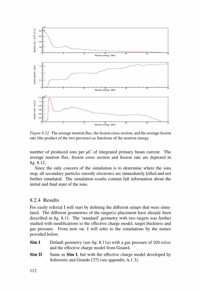
Neutron energy / MeV0 5 10 15 20 25 30

-1C

s)

μ 2

Neutr

on flu

x / (

cm

0

100

200

300

400

610×

Neutron energy / MeV0 5 10 15 20 25 30

Cro

ss s

ection / b

arn

0

0.5

1

1.5

Neutron energy / MeV0 5 10 15 20 25 30

-1C

s)

μF

issio

n r

ate

/ (

0

0.02

0.04

0.06

0.08

0.1

0.12

15−

10×

Figure 8.12. The average neutron flux, the fission cross section, and the average fissionrate (the product of the two previous) as functions of the neutron energy.

number of produced ions per μC of integrated primary beam current. Theaverage neutron flux, fission cross section and fission rate are depicted infig. 8.12.

Since the only concern of the simulation is to determine where the ionsstop, all secondary particles (mostly electrons) are immediately killed and notfurther simulated. The simulation results contain full information about theinitial and final state of the ions.

8.2.4 ResultsFor easily referral I will start by defining the different setups that were simu-lated. The different geometries of the target(s) placement have already beendescribed in fig. 8.11. The ‘standard’ geometry with two targets was furtherstudied with modifications to the effective charge model, target thickness andgas pressure. From now on, I will refer to the simulations by the namesprovided below.

Sim I Default geometry (see fig. 8.11a) with a gas pressure of 200mbarand the effective charge model from Geant4.

Sim II Same as Sim I, but with the effective charge model developed bySchiwietz and Grande [37] (see appendix A.1.3).

112

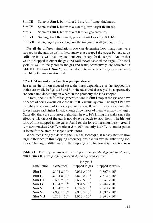
Sim III Same as Sim I, but with a 7.5mg/cm2 target thickness.Sim IV Same as Sim I, but with a 150mg/cm2 target thickness.Sim V Same as Sim I, but with a 400mbar gas pressure.Sim VI Six targets of the same type as in Sim I (see fig. 8.11b).Sim VII A big target pressed against the ion guide wall (see fig. 8.11c).

For all the different simulations one can determine how many ions werestopped in the gas, as well as how many that escaped the target but ended upcolliding into a wall, i.e. any solid material except for the targets. An ion thatwas not stopped in either the gas or a wall, never escaped the target. The totalyield as well as the yields in the gas and walls, respectively, are collected intable 8.1. For Sim I–Sim V, one can also determine how many ions that werecaught by the implantation foil.

8.2.4.1 Mass and effective charge dependenceJust as in the proton-induced case, the mass dependence in the stopped ionyields are small. In figs. 8.13 and 8.14 the mass and charge yields, respectively,are compared depending on where in the geometry the ions stopped.

In total, about 1.91% of the generated ions in Sim I stop in the gas and havea chance of being evacuated to the IGISOL vacuum system. The light FPs havea slightly larger ratio of ions stopped in the gas, than the heavy ones, since thelower charge and higher kinetic energy allow more of them to escape the target.Naturally, there are also more light, than heavy, FPs hitting the walls since theeffective thickness of the gas is not always enough to stop them. The highestratio of ions stopped in the gas is found for the lowest mass numbers. AroundA = 80 it reaches 2.09%, while at A = 160 it is only 1.89%. A similar patteris found for the atomic charge distributions.

When measuring yields with the IGISOL technique, it mostly matters howlarge difference in this stopping efficiency one has for two neighbouring iso-topes. The largest differences in the stopping ratio for two neighbouring mass

Table 8.1. Yields of the produced and stopped ions for the different simulations,Sim I–Sim VII, given per μC of integrated primary beam current.

Ion yieldSimulation Generated Stopped in gas Stopped in wallsSim I 3.104 × 104 5.934 × 102 9.897 × 103

Sim II 3.104 × 104 6.679 × 102 7.372 × 103

Sim III 1.552 × 104 3.569 × 102 9.357 × 103

Sim IV 3.104 × 105 5.981 × 102 9.984 × 103

Sim V 3.104 × 104 1.139 × 103 9.348 × 103

Sim VI 5.300 × 104 9.945 × 102 1.692 × 104

Sim VII 1.241 × 105 1.910 × 103 2.804 × 104

113

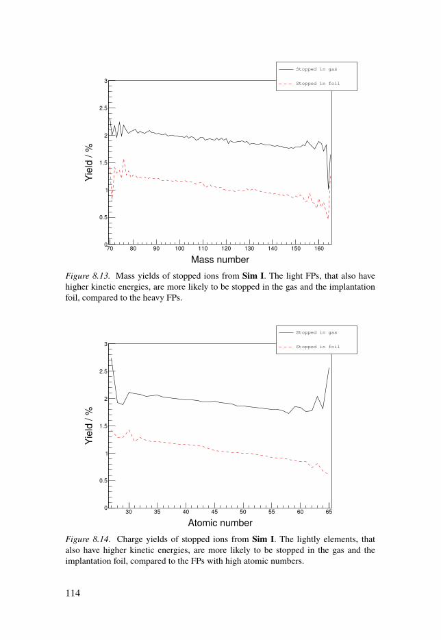
Mass number

70 80 90 100 110 120 130 140 150 160

Yie

ld /

%

0

0.5

1

1.5

2

2.5

3

Stopped in gas

Stopped in foil

Figure 8.13. Mass yields of stopped ions from Sim I. The light FPs, that also havehigher kinetic energies, are more likely to be stopped in the gas and the implantationfoil, compared to the heavy FPs.

Atomic number

30 35 40 45 50 55 60 65

Yie

ld /

%

0

0.5

1

1.5

2

2.5

3

Stopped in gas

Stopped in foil

Figure 8.14. Charge yields of stopped ions from Sim I. The lightly elements, thatalso have higher kinetic energies, are more likely to be stopped in the gas and theimplantation foil, compared to the FPs with high atomic numbers.

114

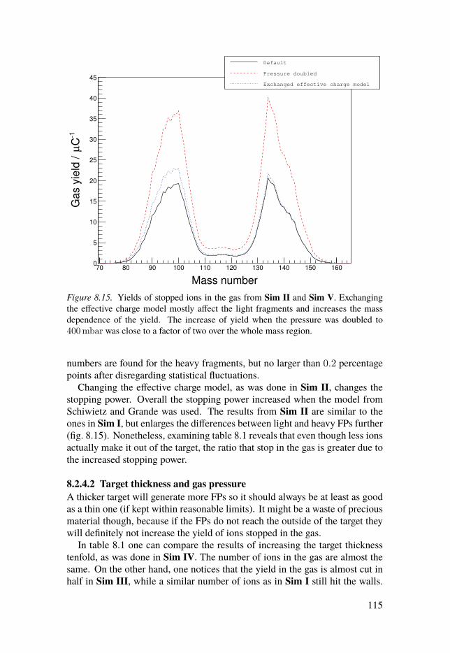
Mass number

70 80 90 100 110 120 130 140 150 160

-1C

μG

as y

ield

/

0

5

10

15

20

25

30

35

40

45

Default

Pressure doubled

Exchanged effective charge model

Figure 8.15. Yields of stopped ions in the gas from Sim II and Sim V. Exchangingthe effective charge model mostly affect the light fragments and increases the massdependence of the yield. The increase of yield when the pressure was doubled to400mbar was close to a factor of two over the whole mass region.

numbers are found for the heavy fragments, but no larger than 0.2 percentagepoints after disregarding statistical fluctuations.

Changing the effective charge model, as was done in Sim II, changes thestopping power. Overall the stopping power increased when the model fromSchiwietz and Grande was used. The results from Sim II are similar to theones in Sim I, but enlarges the differences between light and heavy FPs further(fig. 8.15). Nonetheless, examining table 8.1 reveals that even though less ionsactually make it out of the target, the ratio that stop in the gas is greater due tothe increased stopping power.

8.2.4.2 Target thickness and gas pressureA thicker target will generate more FPs so it should always be at least as goodas a thin one (if kept within reasonable limits). It might be a waste of preciousmaterial though, because if the FPs do not reach the outside of the target theywill definitely not increase the yield of ions stopped in the gas.

In table 8.1 one can compare the results of increasing the target thicknesstenfold, as was done in Sim IV. The number of ions in the gas are almost thesame. On the other hand, one notices that the yield in the gas is almost cut inhalf in Sim III, while a similar number of ions as in Sim I still hit the walls.

115

This means that the thickness in Sim I is close to optimal. The yield does notincrease as a thicker target is used and a thinner target will not be able to, in thesame extent, degrade the energy of the most energetic ions, thereby making itpossible for them to stop within the gas volume.

One way of making the ion guide facilitate a larger yield of ions stoppedin the gas is to make the chamber bigger. However, there might be an easierway. One of the plots in fig. 8.15 represents the yield as the gas pressure isdoubled and thereby effectively making the gas twice as thick. The numbers intable 8.1 shows that the yield in the gas is doubled, more ions are now stoppedbefore they hit any of the walls. Furthermore, one concludes by comparingto the default case in fig. 8.15, that the increased pressure has not affected themass dependence compared to the situation in Sim I. Higher pressure couldbe a good option for increasing the yield, as long as the differential pumpingcan keep a low enough pressure in the vacuum part of IGISOL. Currently, nohigher pressure than 400mbar is possible.

8.2.4.3 Target geometriesOnly the setup of Sim I has up till today been experimentally tried. Althoughthere were plans of realising also a target in the style of Sim VII. The currenttarget holder already has space for up to six targets as in Sim VI. But asthe numbers in table 8.1 show, the benefit of adding extra targets declinesas the distance from the neutron source increases. This can also be seen bycomparing fig. 8.16 to fig. 8.17, where the positions of the stopped ions in thegas are depicted. When all six targets holders are used, the relative number ofevents stopped in the gas originating from the middle and the back targets, areonly 22% and 19%, respectively. This also shows the importance of centringthe targets, because even though further away, the more centred back targetscontributed almost as much as the middle targets.

The target in Sim VII has three major benefits compared to the standardsetup in Sim I. Firstly, it has an area which is 2.6 times greater. Secondly, it iscentred on the neutron beam where the flux is the highest. Lastly, it is as closeas the ion guide allows to the neutron source. All of this combined, result ina 3.2 times higher yield of stopped ions in the gas for Sim VII compared toSim I. In fig. 8.18 the spatial distribution of the stopped ions when using thisbigger target is shown.

Even though there are clearly a higher concentration of stopped ions close tothe targets in figs. 8.16 to 8.18, many of the ions traverses the whole chamber.In fig. 8.19 the cumulative distribution of stopped ions is plotted as a functionof distance from the fission event. The distance is measured perpendicular tothe target surface, which give us an estimate of how much free space is neededin front of each target to maximise the yield. Half the FPs are stopped within14mm of the target, while less than 80% are stopped within 28mm.

116

Figure 8.16. Positions of the ions stopped in the gas from Sim I given per μC ofintegrated primary beam current. Each pixel represents an 0.2mm × 0.2mm area.Most ions are stopped close to the target they originated from.

Figure 8.17. Positions of the ions stopped in the gas from Sim VI given per μC ofintegrated primary beam current. Each pixel represents an 0.2mm × 0.2mm area.The targets in the back is clearly contributing much less than the front ones due to thereduced neutron flux.

117

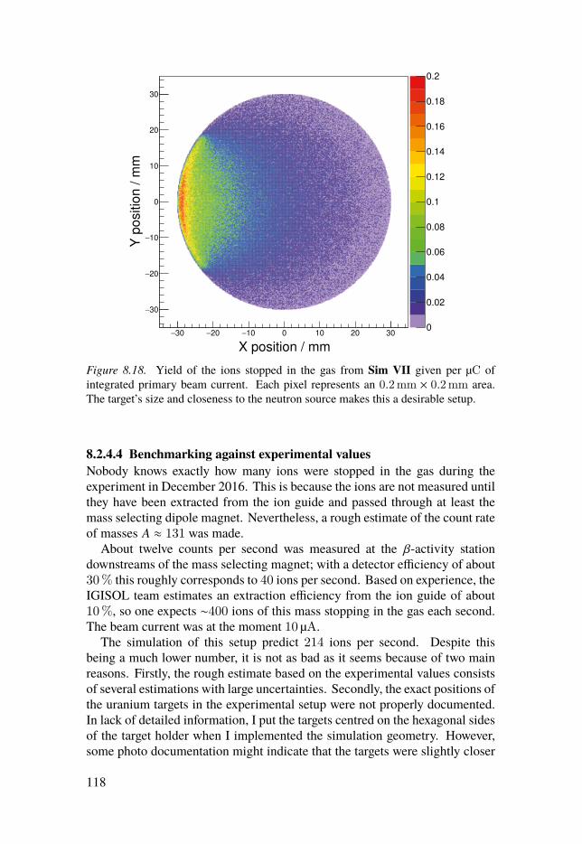
0

0.02

0.04

0.06

0.08

0.1

0.12

0.14

0.16

0.18

0.2

X position / mm30− 20− 10− 0 10 20 30

Y p

ositio

n / m

m

30−

20−

10−

0

10

20

30

Figure 8.18. Yield of the ions stopped in the gas from Sim VII given per μC ofintegrated primary beam current. Each pixel represents an 0.2mm × 0.2mm area.The target’s size and closeness to the neutron source makes this a desirable setup.

8.2.4.4 Benchmarking against experimental valuesNobody knows exactly how many ions were stopped in the gas during theexperiment in December 2016. This is because the ions are not measured untilthey have been extracted from the ion guide and passed through at least themass selecting dipole magnet. Nevertheless, a rough estimate of the count rateof masses A ≈ 131 was made.

About twelve counts per second was measured at the β-activity stationdownstreams of the mass selecting magnet; with a detector efficiency of about30% this roughly corresponds to 40 ions per second. Based on experience, theIGISOL team estimates an extraction efficiency from the ion guide of about10%, so one expects ∼400 ions of this mass stopping in the gas each second.The beam current was at the moment 10 μA.

The simulation of this setup predict 214 ions per second. Despite thisbeing a much lower number, it is not as bad as it seems because of two mainreasons. Firstly, the rough estimate based on the experimental values consistsof several estimations with large uncertainties. Secondly, the exact positions ofthe uranium targets in the experimental setup were not properly documented.In lack of detailed information, I put the targets centred on the hexagonal sidesof the target holder when I implemented the simulation geometry. However,some photo documentation might indicate that the targets were slightly closer

118

Distance from fission / mm

0 10 20 30 40 50 60

Ratio o

f sto

pped ions / %

0

10

20

30

40

50

60

70

80

90

100

Figure 8.19. Cumulative distribution of the how far the stopped ions travelled fromthe fission event perpendicular to the target surface. Only FPs that escape the targetand stop in the gas are taken into account.

to the beam centre. Even a small difference in distance would quickly giverise to a sizeable discrepancy since the neutron flux is much greater toward thebeam centre.

Taken this into account, I conclude that the numbers are in the right orderof magnitude and that more work and detailed documentation is needed fromthe experimental side.

8.2.5 ConclusionsAlso for the neutron induced case one sees that the targets are of reasonablethickness (not surprisingly since they were almost the same thickness). Thickertargets are unnecessary and thinner ones risk introducing a mass dependentstopping efficiency, in addition to simply giving a lower yield. To increase theyield the target surface exposed to the gas must be increased, and the neutronflux through the target optimised. The setup Sim VII represent one way ofdoing this, which could be combined with a higher gas pressure to furtherenhance the yield of stopped ions in the gas. From fig. 8.19 one gets an idea ofhow much free space is needed, in front of each target. Perhaps, can the targetsbe placed closer to each other in a stacked formation as in Fig. 3 in Ref. [111].

119

Increasing the gas pressure showed no effect on the mass distribution ofthe stopped ions. The small dependencies on mass and atomic numbers arenegligible as long as neighbouring isotopes are compared. However, if onewould actually compare, e.g., a very heavy ion to a very light one, the relativedifference would be no more than ∼20%. Chemical effects, e.g. differentcharge-state distributions after the ions are stopped for non-identical elements,might have additional effects which could not be predicted by these simulations.Comparing same-element isotopes is preferred when possible.

Since these new simulations give yield predictions for any FP on an abso-lute scale, they can be verified experimentally. The implantation foil present inSim I, and also in the real experiment conducted in December 2016, will un-dergo a γ-spectroscopy analysis. This will hopefully prove that my simulation-based estimations and predictions have been sound with much less uncertaintiesthan the rough estimate discussed in section 8.2.4.4. Such an analysis shouldalso be able to determine which effective charge model that best reproducesthe experimental results.

These simulations support the methodology employed at IGISOL, and agreewith experimentally based estimates within the (admittedly large) uncertainties.The next step would be to further investigate the charge-state of the fully stoppedions end up in as well as how efficiently the gas flow can carry these ions intothe vacuum part of IGISOL. This is outside the scope of this work, but wouldadd to the knowledge of the ISOL-technique at hand. Nevertheless, the currentdeveloped tools can be used to investigate any new considered geometry, e.g.,bigger chambers with larger gas volume to stop the ions in.

120

9. Svensk sammanfattning (Summary inSwedish)

Ja, det är här uranet förvandlas tillplutonium som vi ska använda tillbränsle i raketen.

— Rymdkraft

Denna avhandlingen behandlar fyra olika projekt som alla handlar om att ökavår förståelse av neutron-inducerade reaktioner genom experimentell kärnfysi-kalisk forskning. En mycket viktig sådan reaktion är fission, dvs. kärnklyvning.Trots att man har kunnat driva kärnkraftverk säkert, i över 60 år, finns det mycketsom fortfarande är okänt gällande exakt hur det går till när en tung atomkärnasplittras till två mindre dotterkärnor. En mer detaljerade diskussion om fis-sionsprocessen ges i avsnitt 2.4. Ökad kunskap om fissionprocessen och bättreuppmätt fissiondata är betydelsefullt för både tillämpningar som kärnkraft,men också för grundforskningen.

För att neutronbaserade experiment överhuvudtaget ska kunna utföras krävsdetektoruppställningar, stora forskningsanläggningar, men ofta även tillgång tilltidigare uppmätt kärndata. Detektorerna som använts diskuteras i kapitel 3 ochanläggningarna där dessa brukats i kapitel 4. Två av mina projekt har handlat oms.k. neutronstandardtvärsnitt som används för att mäta nya reaktionstvärsnittrelativt mot. Det är därmed av yttersta vikt att dessa standarder är mycketprecist bestämda eftersom eventuella fel i standarden kommer att fortplanta sigtill samtliga resultat i sådana relativa mätningar. Dessa standarder och hur deanvänds beskrivs i avsnitt 2.1.

Mitt första projektet som beskrivs i kapitel 5 bestod i ett simuleringsarbetevars mål var att förutsäga hur vår planerade detektoruppställning skulle upp-föra sig i en experimentell situation. Experimentet syftade främst till att mätatre olika neutronstandardtvärsnitt jämtemot varandra och på så sätt minimerasystematiska fel i mätningen. Reaktionerna i fråga var H(n,n), 235U(n,f) och238U(n,f). Själva experimenten har ännu inte utförts eftersom bygget av neu-tronanläggningen Neutrons For Science i Caen (Frankrike) [39, 40] har blivitmångårigt försenat. Dock visade simuleringarna vad för resultat vi kunde för-vänta oss samt vad i utvecklingen av den experimentella uppställningen som viborde fokusera på. Projektet och detektoruppställningen har vid det här lagetutvecklats så pass att nya uppdaterade simuleringar planeras, baserade på dejag tidigare gjorde.

121

Kapitel 6 handlar om mitt andra projekt som också det försökte mäta neu-tronstandarder mot varandra. Denna gång berördes reaktionerna 6Li(n,α)t och235U(n,f) som mättes i en joniseringskammare. Till skillnad från fission är6Li(n,α)t-reaktionen betydligt enklare eftersom endast två produkter skapas.Med hjälp av bevarandet av energi och rörelsemängd kan de två produkter-nas vinklar och energier beräknas analytiskt. Tre upprepade mätningar gjordesvid neutronanläggningen GELINA i Geel (Belgien) [42, 43] i samarbete medEU-laboratoriet JRC-Geel och både uppställning och metodik förbättrades förvarje gång. Många problem löstes men tyvärr lyckades inte heller den sistamätningen att producera goda resultat med små osäkerheter, vilket så klartvar vårt mål. Dock drogs många lärdomar av de problem som uppstod underprojektets gång.

Båda ovan nämnda projekt använde sig av tvärsnittsdata för fissionsreak-tioner för att deducera nya tvärtsnitt för andra reaktioner, men mitt tredjeprojekt handlade om att faktiskt mäta fissionsdata. Även detta projekt varett samarbete mellan Uppsala universitet och JRC-Geel. I kapitel 7 beskrivsutvecklingen av både fissionsspektrometern VERDI [90, 91] och den s.k. 2E-2v-analysmetoden. En av höjdpunkterna med denna metod är att antalet promptemitterade neutroner kan härledas utan att själva neutronerna faktiskt mäts ochutan att ta hjälp av tidigare uppmätt data. Mitt arbete har varit fokuserat påatt kalibrera uppställningen och reproducera tidigare data för 252Cf(sf ). An-vändningen av kiseldetektorer skapar ett flertal komplikationer vilket kräver enicketrivial kalibreringsprocedur pga. det plasma som induceras när de tunga fis-sionprodukterna stoppas i detektorerna. Utvecklingsarbetet pågår fortfarandemen flera framsteg har gjorts och lösningar på identifierade tillkortakomman-den föreslås. En viktig insikt var att tidigare experiment av denna typ intetagit hänsyn till en korrelation mellan den uppmätta fragmentmassan och ne-utronmultipliciteten. Jag utvecklade en enkel korrektionsmetod som även kanappliceras på tidigare uppmätta data från andra grupper.

Det fjärde och sista projektet behandlas i kapitel 8 och är, liksom mitt förstaprojekt, av simuleringskaraktär. Det finländska universitetet i Jyväskylä hand-har en anläggning, vid namn IGISOL [44, 45], som är till för precisa mätningarav fissionproduktsmassor och fissionsproduktsutbyte. Jag har skrivit, utfört ochanalyserat simuleringar i samråd med den experimentella IGISOL-gruppenbåde i Uppsala och Jyväskylä för att sprida ljus över hur många fissionspro-duktsjoner som skapas under experimenten och hur många som förloras påvägen från produktionstället till mätstationen. Fissionsprodukterna skapas iuranfolier antingen genom direkt protonbestrålning eller genom att först skapaen neutronkälla av protonerna och sedan bestråla uranet med neutroner. Endastenstaka procent av dessa tunga joner stoppas sedan upp i buffertgasflödet somtransporterar dem vidare i systemet mot någon av mätstationerna. En av fråge-ställningarna har varit om alla joner stoppas i gasen med samma sannolikhetoberoende av grundämne och massa. Jag kunde konstatera från simuleringarnaatt endast små skillnader beroende på jontyp behöver förväntas. Andra para-

122

metrar undersöktes också, såsom buffertgastrycket och olika sätt att placerastrålmålen på. Jämförelser med experimentell data visade att simuleringarnavar i rimlig överensstämmelse.

123

10. Acknowledgements

A neural transceiver is required formaximum communication, we willwork as one mind.

— Borg collective

Science is not easy if you are all alone, but luckily I have had lots of peoplehelping me throughout my time as a Ph.D student. I will try to list themost significant contributors, but most likely someone has undeservedly beenforgotten (sorry!). I will start by thanking the Swedish Research Council, theCHANDA project, and the EUFRAT transnational access programme for theirfinancial support, since science is so expensive.

I would like to thank all four of my official supervisors at Uppsala Universityfor their support. As my main supervisor C. Gustavsson have given me a lot ofvaluable advice over the years. S. Pomp has provided me with contacts in thenuclear data community and arrangements so that I could work on interestingexperiments. A. Prokofiev has long experience in the field and has an acutesense for details and tough questions. A. Al-Adili has been a great colleagueand a source of incurable optimism, always happy to help, share and discuss.

Two of my projects resided at the European Commission Joint ResearchCentre in Geel, Belgium. It is truly a great place for science and I have learneda lot on each of my visits there. My de facto supervisors in Belgium, F.-J. Hambsch and S. Oberstedt have been welcoming and helpful. Together withA. Göök, they have all been valuable assets that gladly and patiently sharedtheir experience, thoughts and expertise with me. I thank M. Vidali for hisassistance in so many things, T. Gamboni for fixing my vacuum, W. Geerts forfinding me tape, N. Sevenhans for letting me safely in to the experiments, andeveryone else at the JRC who have been of assistance. Although not at JRC-Geel anymore, I thank R. Bevilacqua as well as M. O. Frégeau for introducingme to their previous projects.

Back in Uppsala, some people deserve special thanks, among them: E. An-dersson Sundén and A. Hjalmarsson for their many ideas and the fruitfuldiscussions I have had with them, revolving just about anything. Also thanksto the IGISOL group in Uppsala: M. Lantz, A. Mattera, V. Rakopoulos andA. Solders. They are the ones who do the hard experimental work while I justsimulate it.

Many typos and errors are no longer in this thesis, whereas improvementshave taken their place instead. This is thanks to the proof-reading and reviewing

124

of my manuscript performed by A. Al-Adili, C. Gustavsson, F.-J. Hambsch,A. Solders, S. Oberstedt, A. Prokofiev, and D. Tarrío.

125

Appendix A.Code developed

Am Heimcomputer sitz’ ich hierund programmier’ die Zukunft mir.

— Kraftwerk

In this appendix I have collected short descriptions of codes I have developedthat might be of general interest. They are all available upon request.

A.1 Modifications to Geant4A.1.1 Extended and corrected cross sectionsWhen writing a Geant4 simulation program one can, for a certain physicalprocess, choose which physics model one likes to use depending on the energyregion. For neutron reactions, Geant4 includes a High Precision (HP) modelwhich is driven by data collected from evaluations. However since data is notalways available for higher energies, the model only covers the energy region0 to 20MeV. If one would like to cover a larger energy range, one would needto supplement the HP model with another model and ’stitch‘ them together at20MeV. Sometimes it can be difficult to make a smooth transition from onemodel to the other. One could also try to find a non-data driven model thatworks for the whole interval, but one would then need to rely on theoreticalcalculations or parametrisations rather than experimentally measured data.

Since the simulations described in section 5.3 modelled neutrons up to40MeV, I had to go for one of these options. To capture the cross sectionas accurate as possible I implemented data-driven fission cross sections forthe whole energy range. Normally, this would be somewhat trivial to dowith Geant4, since models describing the physical process are completelyindependent of the models describing cross sections. However, the modelthat was used for inelastic scattering (above 20MeV), the Binary Cascademodel [36, p. 450], treats the fission process on the same footing as inelasticscattering. The fission channel is included in the inelastic scattering model asif it was just another channel of inelastic scattering. In order for me to add anew fission process above 20MeV, I had to remove the fission part from theinelastic model to avoid doubling the fission event rate. After that I added a

126

Neutron energy (MeV)0 5 10 15 20 25 30 35 40

Nu

mb

er

of

co

un

ts (

a.u

.)

0.2

0.4

0.6

0.8

1HP + CHIPS

Corrected

Figure A.1. The histogram shows the counts of simulated recoil protons from elasticneutron scattering on hydrogen versus incident neutron energy. The results shown bythe solid curve were obtained when the simulation was using default Geant4 classes.The dashed curve shows the result after new cross sections were supplied.

new model with my own data-driven cross sections based on the IAEA neutronstandards evaluations [112].

I also had to implement new cross section for elastic scattering since Idiscovered non-physical structures in the default cross section (CHIPS para-metrisation [36, p. 388]). For elastic scattering one expects a smooth behaviourof the cross section as a function of energy [9, 113, 114], but this was not thecase as showcased in fig. A.1. The change of cross section data could bedone in a straight-forward way due to Geant4’s support of adding cross sectionindependently of the physics models. In Fig. A.1 I show the difference beforeand after my cross-section fix. The curve obtained when the simulation wasusing cross sections provided by unmodified Geant4 classes (HP in the range 0to 20MeV and CHIPS above 20MeV) exhibits a structure in the energy range20 to 35MeV. After substituting the CHIPS parametrisation with additionaldata from evaluations [113] the expected smooth behaviour was restored.

A.1.2 Biasing of discrete events in simulationsIn order to save time while doing a simulation starting from the incomingneutron, custom code that scaled up certain cross sections and weighted theparticles accordingly was implemented. Current versions of Geant4 now in-clude this functionality through default classes, but at the time the simulationsoftware discussed in section 5.3 was written, they did not.

127

This custom implementation of cross-section scaling within Geant4 simu-lations is similar to the one described by Mendenhall and Weller [115]. Thescaling factor, the process to be biased and the geometrical regions in whichthe scaling occurs, are all configurable through a messenger helper class ac-companying the main class.

The new class, BiasedProcess, inherits G4WrapperProcess and wrapsdiscrete processes. It works by substituting the original process with thewrapper process. When the wrapper process is called by Geant4, it willforward the call to the original process. In the case when Geant4 asks itto calculate the interaction length, the wrapper process will use the originalprocess to calculate the unbiased interaction length. Before returning this valueto Geant4 it will divide the unbiased interaction length with a biasing factorthus scaling the cross section.

To compensate the biasing, each event is given a weight. If no biasing is donethis weight will be unity. If we e.g. scale the fission cross section upwards,the weight for fission events will be lower than unity. On the other hand, everydistance the particle travels without any fission occurring will increase theparticle weight. After each step in a region where biasing is applied the weightis adjusted accordingly.

When the biased interaction occurs, the weight is linearly scaled by thebiasing factor b. The new weight is given by

wnew =wold

b, (A.1)

where wold and wnew denotes the weights before and after the interaction,respectively. A particle travelling the distance Δx through a region with abiased process adjusts its weight by an exponential factor. This time the newweight is given by

wnew = wold exp

( (b − 1)Δx�

), (A.2)

where � denotes the (unbiased) mean free path. Eq. A.1 and A.2 ensure thatthe product of the probability and the weight is kept constant, no matter whatbiasing factor is used.

If we assume that we use the biasing to make the occurrence of an unusualevent to become more likely in the simulations, i.e. b > 1, Eq. A.1 woulddecrease the weight whenever the biased event happens, compensating theincreased rate in the simulation of this kind of event. Similarly, Eq. A.2 wouldincrease the weight if the particle just passes by and no interaction of that kindoccurs.

Every particle in the simulations carries a weight but BiasedProcess keepstrack of the accumulated weight for the whole event, i.e. everything that happenin the simulation due to one primary particle. The resulting weight of the fullevent is saved together with the rest of the event data. The event weight is a

128

measure of the likeliness of the event as a whole, taking all biased reactionsinto account.

All biasing options can be specified at the command prompt or in a macroat any time before the simulation starts. One specifies the biasing factor, b,and the biased particle type as well as any number of G4VPhysicalVolumeinstances where the bias should be activated. One can also choose whetheronly the primary particle should be biased or secondaries as well. To avoidevents with very low weights (w < 1/b) yet another option exists to limit thebiasing to never go below a certain limit.

This class was tested and used for the simulations described in section 5.3.Fission as well as elastic and inelastic scattering have been biased to gethigher statistics more efficiently. The most highly biased processes in thiswork were using a biasing factor of 1000. However, the track of a non-reactingneutron requires little time to be calculated, compared to the case where severalsecondary particles are produced by reactions induced by the primary particle.Therefore, the CPU time reduction when using biasing was usually not morethan an order of magnitude, compared to the non-biased case. If the unbiasedreactions are more time-consuming to simulate, the potential benefits of biasingmight increase.

A.1.3 New effective charge modelAs was mentioned in section 3.4.2 the effective charge of an ion affect thestopping power greatly. By default Geant4 parametrises the effective charge asa function of the atomic numbers of the projectile, the atomic number of thebulk material, and the projectile velocity [36]. The exact expression is basedon the work of Brandt and Kitagawa [116]. However, newer parametrisationsexist and heavy ion stopping powers are still not accurately known. Schiwietzand Grande fitted expressions to available experimental data for both gaseousand solid materials, respectively [37]. While the parameters are the same, thefunctional form is different.

Implementing a new charge-state formula in Geant4, based on the parametervalues found by Schiwietz and Grande, turned out to be not so difficult. Thewhole calculation is contained within the class G4ionEffectiveCharge butthe Geant4 authors did not provide a simple way of substitute it with yourown custom class. Among other things many methods in relevant classes werenot declared virtual. In order to minimise the intrusion to the Geant4 code,I instead modified the class G4ionEffectiveCharge directly in the Geant4(version 10.01.p03) source tree to include an option to use the Schiwietzand Grande parametrisation instead. The default option was still available,so the user could easily switch between the two options through a macroscommand to compare how the different charge models affect the simulationresults. Generally, the Schiwietz and Grande parametrisation yields higher

129

charges and therefore shorter stopping ranges, which was observed in theIGISOL simulations reported on in chapter 8.

A.2 ROOT file I/O made simpleThe ROOT Data Analysis Framework is a commonly used library withinexperimental nuclear physics. Among other things it specifies its own fileformat and data structures which are designed to store experimental, simulatedor analysed data, event by event. Instead of writing almost the same code overand over again in all my different analysis projects, I decided to write a C++class that took care of it once and for all. My class wraps the storing processand provides a simpler and more fool proof interface to the user.

Since simplicity was preferred over technical elegance, the class RootFile-Manager was designed as a singleton class, reachable from anywhere in thecode through a static member method. I restricted it to only handle one file ata time since I never had a use for more than that. To use it in a project, the userfirst needs to initialise it by specifying the output file and what kind of datawill be stored in the file for each event. A handle for each data slot is returnedand will be the key to store the correct data in the correct slot. This is quiteliterally so, because the handle is internally used as the key in a binary tree tofind the correct storage. The following code would create a new event tree andpreparing it to store two variables for each event, one 64-bit integer named Aand one low precision floating point value named B, respectively.

Example codeRootFileManager* rfm = RootFileManager::Instance();rfm->OpenFile("output.root");handle my_tree = rfm->NewTree("MyEvents");handle my_a = rfm->NewInt64(my_tree,"A");handle my_b = rfm->NewFloat32(my_tree,"B");

Note that ROOT calls its event data structure a ’tree‘, but it is not a binarytree as one might suspect. It is possible to work with any number of trees inparallel. Later on when our example program, e.g., has acquired one event.The important values a and b are saved by calling the different Fill methodsof RootFileManager followed by a call to CloseEntry():

Example coderfm->FillInt(my_tree,a);rfm->FillFloat(my_tree,b);rfm->CloseEntry();

Nothing is actually written to the output file until the last call, but rather keptin buffers. Calling CloseEntry(my_tree) will store the current content of

130

the buffers corresponding to the particular event tree that is specified throughthe supplied handle my_tree. When all events has been processed the file isclosed by a call to CloseFile(), but that can also be left to be handled by thedestructor if it also the end of the program.

The primitive data types that can be saved are integers and floating pointvalues, of either 32 bits or 64 bits. One can also specify that one likes to store anarbitrary long vector of these primitive types for each event. In addition one canalso save strings, graphs and arrays of objects as long as they inherit from theRoot main class TObject. It is also possible to store any TObject descendantdirectly, outside the event structure, but possibly in a folder hierarchy.

The versatility and ease of use proved the initial effort to write the classworth it, it has been used in every single project presented in this thesis (and afew others).

A.3 Acquisition software for a SPdevices digitiserA few years back our laboratory was equipped with a new SPdevices digitiser(model ADQ412). Since we lacked a suitable easy to use acquisition program,especially any that ran on Linux systems, I wrote a new one from scratch.

The acquisition program runs from a command line interface either ininteractive or batch mode. It was written with minimalism in mind and hasno dependencies except for the C++11 standard library and the provided APIfrom SPdevices. All important configuration options can be set in a simpletext file supplied at the command line. The user can choose the output file(s)and how large they should be, as well as if the program should terminate aftera certain number of events. It can also be run in a ’waiting‘ mode where itacquires a number of events and then wait for the user to make adjustments onthe experimental setup before collecting the next set of events.

The device itself is connected with a USB cable to a normal PC, it featuresfour 12-bit precision channels and a sample rate of 1GHz. By using onlytwo of the channels in a so called interleaving mode, the sample rate can bedoubled. Each event will be collected as the detector voltage level crosses apreset threshold. Which of the channels that will be stored to disk, as well aswhich can trigger acquisition, are configurable. The total size of the trace aswell as the number of samples before the trigger, are also chosen before theacquisition starts. A few more options, like configurable DC-offsets for eachchannel, is also available.

The output format is a binary file with a fixed sized header containinginformation about the specific acquisition. The header mostly contains theconfiguration parameters given to the digitiser, as well as the acquisition dateand total time of the acquisition. After the header, all event traces for all activechannels are stored subsequently. Each with a timestamp indicating exactlywhen the event occurred.

131

The program has proven useful since it has been used by several groups andis now at version 6. After me being the only developer for a long time, it is nowcontinuously developed by several people. It runs on Linux and most likelyalso on Windows (but this has not been tested). It only supports the ADQ412model, but adaptations to other SPdevices digitisers should be easy.

132

Appendix B.Selected publications

Time moves in one direction, memoryanother. We are that strange speciesthat constructs artifacts intended tocounter the natural flow of forgetting.

— William Gibson

Published full length papers

I Two level scheme solvers for nuclear spectroscopyK. Jansson, D. DiJulio, J. Cederkäll, Nucl. Instrum. Meth. A 654 (2011)496–501, doi:10.1016/j.nima.2011.07.021My contribution:Designed, implemented and analysed the algorithms, wrote thepaper, based on my master’s thesis.

II Designing an upgrade of the Medley setup for light-ionproduction and fission cross-section measurementsK. Jansson, C. Gustavsson, A. Al-Adili , A. Hjalmarsson, E. Andersson-Sundén,A. V. Prokofiev, D. Tarrío, S. Pomp, Nucl. Instrum. Meth. A, 794 (2015) 141–150, doi:10.1016/j.nima.2015.05.001My contribution:Wrote the software, performed the analysis, wrote the paper.

III Simulations of the fission-product stopping efficiency inIGISOLA. Al-Adili, K. Jansson, M. Lantz, A. Solders, D. Gorelov, C. Gustavsson,A. Mattera, I. Moore, A. V. Prokofiev, V. Rakopoulos, H. Penttilä,D. Tarrío, S. Wiberg, M. Österlund, S. Pomp, EPJ A 51 5 (2015) 59,doi:10.1140/epja/i2015-15059-2My contribution:Wrote the simulation software, participated in the analysis andpaper writing.

133

IV Estimates of the production rates of exotic nuclei from the ion-guide for neutron induced fission at IGISOLK. Jansson, A. Al-Adili, N. Nilsson, M. Norlin, A. Solders, Submitted to EPJA (2017), doi: N/AMy contribution:Wrote the main simulation software, performed the analysis,wrote the paper.

V Defective fission correlation data from the 2E-2v methodK. Jansson, A. Al-Adili, E. Andersson Sundén, A. Göök, S. Oberstedt, S. Pomp,Submitted to Phys. Rev. C (2017), doi: N/AMy contribution:Wrote all software, performed the analysis, wrote the paper.

Published conference proceedings

VI Measuring Light-ion Production and Fission Cross SectionsNormalised to H(n,p) Scattering at the Upcoming NFS FacilityK. Jansson, C. Gustavsson, S. Pomp, A. V. Prokofiev, G. Scian, D. Tarrío,Nuclear Data Sheets 119 (2014) 395–397, doi:10.1016/j.nds.2014.08.110My contribution: Performed the simulations and the analysis, wrote the paper.

VII Light-ion Production from O, Si, Fe and Bi Induced by 175 MeVQuasi-monoenergetic NeutronsR. Bevilacqua, S. Pomp, K. Jansson, C. Gustavsson, M. Österlund, V. Simutkin,M. Hayashi, S. Hirayama, Y. Naitou, Y. Watanabe, A. Hjalmarsson,A. Prokofiev, U. Tippawan, F.-R. Lecolley, N. Marie, S. Leray, J.-C. David, S. Mashnik, Nuclear Data Sheets 119 (2014) 190–193,doi:10.1016/j.nds.2014.08.053My contribution: Produced integrated cross sections.

VIII Measurement of the 6Li(n,α) neutron standard cross-sectionat the GELINA facilityK. Jansson, A. Al-Adili, R. Bevilacqua, C. Gustavsson, F.-J. Hambsch,S. Pomp, M. Vidali, EPJ Web Conf. 122 (2016) 08006,doi:10.1051/epjconf/201612208006My contribution:Analysed the data, wrote the paper.

134

IX Analysis of prompt fission neutrons in 235U(nth,f) and fissionfragment distributions for the thermal neutron induced fissionof 234UA. Al-Adili, D. Tarrío, F.-J. Hambsch, A. Göök, K. Jansson, A. Solders,V. Rakopoulos, C. Gustafsson, M. Lantz, A. Mattera, S. Oberstedt,A.V. Prokofiev, M. Vidali, M. Österlund, S. Pomp, EPJ Web Conf. 122 (2016)01007, doi:10.1051/epjconf/201612201007My contribution: Participated in the 235U(nth,f) experiment, assisted the analysis.

X Measurement of the 6Li(n,α)t neutron standard cross-sectionat the GELINA facilityK. Jansson, A. Al-Adili, R. Bevilacqua, C. Gustavsson, F.-J. Hambsch,S. Pomp, M. Vidali, EPJ Web Conf. 146 (2017) 11047,doi:10.1051/epjconf/201714611047My contribution:Analysed the data, wrote the paper.

XI The new double energy-velocity spectrometer VERDIK. Jansson, M. O. Frégeau, A. Al-Adili, A. Göök, C. Gustavsson, F.-J. Hambsch, S. Oberstedt, S. Pomp, EPJ Web Conf. 146 (2017) 04016,doi:10.1051/epjconf/201714604016My contribution:Analysed the data, wrote the paper together with M. O. Frégeau.

XII Simulations of the stopping efficiencies of fission ion guidesA. Solders, A. Al-Adili, D. Gorelov, K. Jansson, A. Jokinen, V. Kolhinen,M. Lantz, A. Mattera, I. Moore, N. Nilsson, M. Norlin, H. Penttilä, S. Pomp,A. V. Prokofiev, V. Rakopoulos, S. Rinta-Antila, V. Simutkin, and the IGISOLgroup, EPJ Web Conf. 146 (2017) 03025, doi:10.1051/epjconf/201714603025My contribution:Wrote the simulation software, co-supervised the student projectperforming the analysis.

XIII Neutron-multiplicity experiments for enhanced fissionmodellingA. Al-Adili, D. Tarrío, F.-J. Hambsch, A. Göök, K. Jansson, A. Solders,V. Rakapoulos, C. Gustavsson, M. Lantz, A. Mattera, S. Oberstedt,A. V. Prokofiev, E. Andersson Sundén, M. Vidali, M. Österlund, S. Pomp,EPJ Web Conf. 146 (2017) 04056, doi:10.1051/epjconf/201714604056My contribution: Participated in the experiment, assisted the analysis.

135

References

[1] O. Hahn and F. Strassmann, Naturwissenschaften 27, 11 (1939) 10.1007/BF01488241.

[2] L. Meitner and O. R. Frisch, Nature 143 (1939) 10.1038/143239a0.[3] W. Moomaw et al., Annex II: Methodology. In IPCC Special Report on

Renewable Energy Sources and Climate Change Mitigation, edited byO. Edenhofer et al. (Cambridge University Press, 2011), http://www.ipcc-wg3.de/report/IPCC_SRREN_Annex_II.pdf.

[4] IPCC, Climate Change 2014: Mitigation of Climate Change. Contri-bution of Working Group III to the Fifth Assessment Report of theIntergovernmental Panel on Climate Change, edited by O. Edenhoferet al. (Cambridge University Press, 2014), https://www.ipcc.ch/pdf/assessment-report/ar5/wg3/ipcc_wg3_ar5_full.pdf.

[5] K. Jansson, Improving the Neutron Cross-section Standards 238U(n,f)and 6Li(n,α), Licentiate thesis, (Uppsala, 2015), http://uu.diva-portal.org/smash/get/diva2:821395/FULLTEXT01.pdf.

[6] M. Sarsour et al., Phys. Rev. Lett. 94, 082303 (2005) 10.1103/PhysRevLett.94.082303.

[7] A. D. Carlson, Metrologia 48, S328 (2011) 10.1088/0026-1394/48/6/S09.

[8] STANDARDS Data development project, Accessed: 2017-06-01, https://www-nds.iaea.org/standards.

[9] V. G. J. Stoks et al., Phys. Rev. C 48, 792 (1993) 10.1103/PhysRevC.48.792.

[10] H. Conde, ed., Nuclear Data Standards for Nuclear Measurements1991 NEANDC/INDC Nuclear Standards File, 1992, https : / /www.oecd-nea.org/science/docs/1991/neandc1991-311-u.pdf.

[11] O. Wasson and R. Schrack, Nucl. Instrum. Meth. A 282, 194 (1989)10.1016/0168-9002(89)90140-X.

[12] W. Pauli, Zeitschrift für Physik 31, 765 (1925) 10.1007/BF02980631.[13] R. Krücken, Contemp. Phys. 52, 101 (2011) 10.1080/00107514.2010.

509993.[14] J. P. Schiffer et al., Phys. Rev. Lett. 92, 162501 (2004) 10 . 1103 /

PhysRevLett.92.162501.

136

[15] K.-H. Schmidt et al., Nucl. Phys. A 665, 221 (2000) 10.1016/S0375-9474(99)00384-X.

[16] K.-H. Schmidt et al., Nucl. Data Sheets 131, Special Issue on NuclearReaction Data, 107 (2016) 10.1016/j.nds.2015.12.009.

[17] V. Strutinsky, Nucl. Phys. A 95, 420 (1967) 10.1016/0375-9474(67)90510-6.

[18] P. Möller et al., Phys. Rev. C 79, 064304 (2009) 10.1103/PhysRevC.79.064304.

[19] U. Brosa et al., Phys. Rep. 197, 167 (1990) 10.1016/0370-1573(90)90114-H.

[20] J. Randrup and P. Möller, Phys. Rev. Lett. 106, 132503 (2011) 10.1103/PhysRevLett.106.132503.

[21] N. Metropolis et al., J. Chem. Phys. 21, 1087 (1953) 10 . 1063 / 1 .1699114.

[22] N. Bohr, Phys. Rev. 58, 864 (1940) 10.1103/PhysRev.58.864.[23] A. Stolarz et al., Nucl. Instrum. Meth. A 613, 351 (2010) 10.1016/j.

nima.2009.09.074.[24] L. Zhang et al., Nucl. Instrum. Meth. B 267, 3480 (2009) 10.1016/j.

nimb.2009.08.005.[25] R. Bevilacqua et al., Nucl. Instrum. Meth. A 770, 64 (2015) 10.1016/

j.nima.2014.10.003.[26] W. Shockley, J. Appl. Phys. 9, 635 (1938) 10.1063/1.1710367.[27] A. Al-Adili et al., Nucl. Instrum. Meth. A 624, 684 (2010) 10.1016/j.

nima.2010.09.126.[28] A. Göök et al., Nucl. Instrum. Meth. A 664, 289 (2012) 10.1016/j.

nima.2011.10.052.[29] G. Hempel et al., Nucl. Instrum. Meth. A 131, 445 (1975) 10.1016/

0029-554X(75)90432-2.[30] H. Hui et al., Nucl. Instrum. Meth. A 481, 160 (2002) 10.1016/S0168-

9002(01)01333-X.[31] D. Tarrío et al., Nucl. Instrum. Meth. A 743, 79 (2014) 10.1016/j.nima.

2013.12.056.[32] T. Gys, Nucl. Instrum. Meth. A 787, New Developments in Photode-

tection NDIP14, 254 (2015) 10.1016/j.nima.2014.12.044.[33] Q. Zhang et al., Rev. Sci. Instrum. 81, 073112 (2010) 10 .1063 / 1 .

3463690.[34] G. F. Knoll, Radiation detection and measurement, 4th (John Wiley &

Sons Inc., 2010), 830 pp., isbn: 0470131489.

137

[35] G. Lutz, Semiconductor radiation detectors (Springer-Verlag BerlinHeidelberg, 2001), 10.1007/978-3-540-71679-2.

[36] Physics reference manual, v. 9.6.0, Geant4 collaboration (2012), http://geant4.web.cern.ch/geant4/UserDocumentation/UsersGuides/PhysicsReferenceManual/BackupVersions/V9.6/fo/PhysicsReferenceManual.pdf.

[37] G. Schiwietz and P. Grande, Nucl. Instrum. Meth. B 175, 125 (2001)10.1016/S0168-583X(00)00583-8.

[38] H. W. Schmitt et al., Phys. Rev. 137, B837 (1965) 10.1103/PhysRev.137.B837.

[39] Ledoux, X. et al., EPJ Web Conf. 146, 03003 (2017) 10.1051/epjconf/201714603003.

[40] X. Ledoux et al., Technical proposal for the spiral 2 instrumentation,2008, pro . ganil - spiral2 . eu / spiral2 / instrumentation / nfs / working -documents/nfs-technical-report.

[41] M. Lewitowicz, Nucl. Phys. A 805, INPC 2007 Proceedings of the23rd International Nuclear Physics Conference, 519c (2008) 10.1016/j.nuclphysa.2008.02.290.

[42] Institute for Reference Materials and Measurements (Geel), Unit Stand-ards for Nuclear Safety, Security and Safeguards, EUFRAT NUCLEARFACILITIES AT JRC-IRMM, Accessed: 2017-07-27, https://ec.europa.eu/jrc/sites/default/files/eufrat-facilities.pdf.

[43] European Commission, Joint Research Centre, Linear electron accel-erator facility, Accessed: 2017-07-27, https : / / ec .europa.eu/ jrc /en/research-facility/linear-electron-accelerator-facility.

[44] Penttilä, H. et al., EPJ A 52, 104 (2016) 10.1140/epja/i2016-16104-4.[45] J. Äystö et al., Hyperfine Interactions 223, 1 (2014) 10.1007/s10751-

013-0872-z.[46] A. Mattera et al., EPJ A 53, 173 (2017) 10.1140/epja/i2017-12362-x.[47] A. Mattera et al., ‘Production of Sn and Sb isotopes in high-energy

neutron induced fission of nat U’, Submitted to EPJ A, 2017.[48] V. Kolhinen et al., Nucl. Instrum. Meth. A 528, 776 (2004) 10.1016/j.

nima.2004.05.029.[49] U. Tippawan et al., Phys. Rev. C 79, 064611 (2009) 10.1103/PhysRevC.

79.064611.[50] R. Bevilacqua et al., Nucl. Instrum. Meth. A 646, 100 (2011) 10.1016/

j.nima.2011.04.036.[51] S. Pomp et al., EPJ Web Conf. 8, 07013 (2010) 10 .1051 / epjconf /

20100807013.

138

[52] K. Jansson et al., Nucl. Data Sheets 119, 395 (2014) 10.1016/j.nds.2014.08.110.

[53] K. Jansson et al., Nucl. Instrum. Meth. A 794, 141 (2015) 10.1016/j.nima.2015.05.001.

[54] I. Slypen et al., Radiat. Prot. Dosim. 70, 21 (1997) 10.1093/oxfordjournals.rpd.a031945.

[55] S. Benck et al., Phys. Med. Biol. 43, 3427 (1998) 10 .1088 / 0031 -9155/43/12/003.

[56] S. Benck et al., Nucl. Sci. Eng. 141, 55 (2002) 10 .13182/NSE02-A2266.

[57] I. Slypen et al., J. Phys. G: Nucl. Part. Phys. 30, 45 (2004) 10.1088/0954-3899/30/2/005.

[58] JEDEC Solid State Technology Association, JEDEC Standard, (2006).[59] D. Jones and A. Wambersie, Nucl. Instrum. Meth. A 580, Proceedings

of the 10th International Symposium on Radiation Physics ISRP 10,522 (2007) 10.1016/j.nima.2007.05.220.

[60] M. Gilbert et al., J. Nucl. Mater. 442, S755 (2013) 10.1016/j.jnucmat.2013.03.085.

[61] P. Beck, Radiat. Prot. Dosim. 136, 244 (2009) 10.1093/rpd/ncp158.[62] C. Zeitlin et al., Science 340, 1080 (2013) 10.1126/science.1235989.[63] P. J. Griffin et al., IEEE Trans. Nucl. Sci. 59, 1167 (2012) 10.1109/

TNS.2012.2193900.[64] P. Lisowski et al., Proceedings of the Specialists’ Meeting on Neutron

Cross Section Standards for the Energy Range Above 20 MeV (Uppsala,Sweden) (1991).

[65] O. Shcherbakov et al., J. Nucl. Sci. Technol. 39, 230 (2002) 10.1080/00223131.2002.10875081.

[66] C. Paradela et al., Phys. Rev. C 91, 024602 (2015) 10.1103/PhysRevC.91.024602.

[67] R. Nolte et al., Nucl. Sci. Eng. 156, 197 (2007) 10.13182/NSE06-14.[68] Tarrío, Diego et al., EPJ Web Conf. 146, 03026 (2017) 10 . 1051 /

epjconf/201714603026.[69] M. Hayashi et al., EDP Sciences, 1091 (2007) 10.1051/ndata:07747.[70] D. Tarrío, ‘Neutron-induced fission fragment angular distribution at

CERN n_TOF: The Th-232 case’, PhD thesis (University of Santiagode Compostela, 2012), https://cds.cern.ch/record/1474269.

[71] S. Agostinelli et al., Nucl. Instrum. Meth. A 506, 250 (2003) 10.1016/S0168-9002(03)01368-8.

139

[72] Geant4 collaboration, Reference Physics Lists, Accessed: 2017-06-01,http : / / geant4 . cern . ch / support / proc _ mod _ catalog / physics _ lists /referencePL.shtml.

[73] A. Breskin and N. Zwang, Nucl. Instrum. Meth. 144, 609 (1977) 10.1016/0029-554X(77)90034-9.

[74] L. Audouin et al., EDP Sciences, 421 (2008) 10.1051/ndata:07675.[75] R. Bevilacqua et al., Nucl. Data Sheets 119, 104 (2014) 10.1016/j.nds.

2014.08.029.[76] K. Jansson et al., EPJ Web Conf. 122, 08006 (2016) 10.1051/epjconf/

201612208006.[77] Jansson, Kaj et al., EPJ Web Conf. 146, 11047 (2017) 10.1051/epjconf/

201714611047.[78] D. Tilley et al., Nucl. Phys. A 708, 3 (2002) 10.1016/S0375-9474(02)

00597-3.[79] G. Zhang et al., Nucl. Instrum. Meth. A 566, 615 (2006) 10.1016/j.

nima.2006.06.064.[80] M. Devlin et al., AIP Conf. Proc. 1090, 215 (2009) 10.1063/1.3087015.[81] M. Chadwick et al., Nucl. Data Sheets 112, Special Issue on ENDF/B-

VII.1 Library, 2887 (2011) 10.1016/j.nds.2011.11.002.[82] R. Bencardino et al., Nucl. Sci. Eng. 177, 68 (2014) 10.13182/NSE13-

25.[83] J. F. Ziegler et al., Nucl. Instrum. Meth. B 268, 19th International

Conference on Ion Beam Analysis, 1818 (2010) 10.1016/j.nimb.2010.02.091.

[84] J. H. Hubbell and S. M. Seltzer, Tables of X-Ray Mass AttenuationCoefficients and Mass Energy-Absorption Coefficients (version 1.4),tech. rep. NISTIR 5632, Accessed: 2017-05-19 (National Institute ofStandards and Technology, Gaithersburg, MD, 2004), physics.nist.gov/xaamdi.

[85] F.-J. Hambsch and I. Ruskov, Nucl. Sci. Eng. 156, 103 (2007).[86] T. Nagy et al., Nucl. Instrum. Meth. 8, 327 (1960) 10.1016/S0029-

554X(60)80030-4.[87] A. Andronic et al., Nucl. Instrum. Meth. A 523, 302 (2004) 10.1016/j.

nima.2003.11.426.[88] H. Bai et al., Nucl. Instrum. Meth. A 840, 36 (2016) 10.1016/j.nima.

2016.09.049.[89] H.-H. Knitter et al., Nuclear Data for Science and Technology: Proceed-

ings of the International Conference Antwerp 6–10 September 1982,451 (1983) 10.1007/978-94-009-7099-1_97.

140

[90] M. Frégeau et al., Nucl. Instrum. Meth. A 817, 35 (2016) 10.1016/j.nima.2016.02.011.

[91] Jansson, Kaj et al., EPJ Web Conf. 146, 04016 (2017) 10.1051/epjconf/201714604016.

[92] R. Müller et al., Phys. Rev. C 29, 885 (1984) 10.1103/PhysRevC.29.885.

[93] K. Nishio et al., J. Nucl. Sci. Technol. 32, 404 (1995) 10.1080/18811248.1995.9731725.

[94] G. Audi et al., Chinese Phys. C 36, 1287, 1287 (2012) 10.1088/1674-1137/36/12/002.

[95] M. Wang et al., Chinese Phys. C 36, 1603, 1603 (2012) 10.1088/1674-1137/36/12/003.

[96] W. Bohne et al., Nucl. Instrum. Meth. A 240, 145 (1985) 10.1016/0168-9002(85)90398-5.

[97] R. Yanez, Range – the -dE/dx and range C/C++ library, version 0.1.5,http://www.calel.org/range.html.

[98] A. Göök et al., Phys. Rev. C 90, 064611 (2014) 10.1103/PhysRevC.90.064611.

[99] J. Velkovska and R. McGrath, Nucl. Instrum. Meth. A 430, 507 (1999)10.1016/S0168-9002(99)00225-9.

[100] K.-T. Brinkmann et al., Nucl. Instrum. Meth. A 276, 557 (1989) 10.1016/0168-9002(89)90583-4.

[101] K. Meierbachtol et al., Nucl. Instrum. Meth. A 788, 59 (2015) 10.1016/j.nima.2015.02.032.

[102] D. Doré et al., Nucl. Data Sheets 119, 346 (2014) 10.1016/j.nds.2014.08.095.

[103] J. Matarranz et al., Physics Procedia 47, Scientific Workshop on Nuc-lear Fission Dynamics and the Emission of Prompt Neutrons andGamma Rays, Biarritz, France, 28-30 November 2012, 76 (2013)10.1016/j.phpro.2013.06.012.

[104] A. Solders et al., Nuclear Data Sheets 119, 338 (2014) 10.1016/j.nds.2014.08.093.

[105] G. Lhersonneau et al., EPJ A 9, 385 (2000) 10.1007/s100500070023.[106] J. Van Schelt et al., Phys. Rev. Lett. 111, 061102 (2013) 10 .1103/

PhysRevLett.111.061102.[107] A. Al-Adili et al., EPJ A 51, 59 (2015) 10.1140/epja/i2015-15059-2.[108] A. Al-Adili et al., (2014), arXiv:1409.0714 [nucl-ex].

141

[109] D. Gorelov et al., Nucl. Instrum. Meth. B 376, 46 (2016) 10.1016/j.nimb.2016.02.049.

[110] G. W. McKinney et al., Proceedings of the MC2005 Conference, Chat-tanooga, Tennessee, April 17-21, 2005, LA-UR-04-8695 (2004).

[111] P. Constantin et al., Nucl. Instrum. Meth. B 397, 1 (2017) 10.1016/j.nimb.2017.02.032.

[112] A. Carlson et al., Nucl. Data Sheets 110, Special Issue on NuclearReaction Data, 3215 (2009) 10.1016/j.nds.2009.11.001.

[113] A. Santamarina et al., The JEFF-3.1.1 Nuclear Data Library, tech. rep.22 (Nuclear Energy Agency, 2009).

[114] Theoretical High Energy Physics Group of the Radboud UniversityNijmegen, NN-Online, Accessed: 2017-08-14, http://nn-online.org.

[115] M. Mendenhall and R. Weller, Nucl. Instrum. Meth. A 667, 38 (2012)10.1016/j.nima.2011.11.084.

[116] W. Brandt and M. Kitagawa, Phys. Rev. B 25, 5631 (1982) 10.1103/PhysRevB.25.5631.

142

Acta Universitatis UpsaliensisUppsala Dissertations from the Faculty of ScienceEditor: The Dean of the Faculty of Science

1–11: 1970–197512. Lars Thofelt: Studies on leaf temperature recorded by direct measurement and

by thermography. 1975.13. Monica Henricsson: Nutritional studies on Chara globularis Thuill., Chara zey-

lanica Willd., and Chara haitensis Turpin. 1976.14. Göran Kloow: Studies on Regenerated Cellulose by the Fluorescence Depolar-

ization Technique. 1976.15. Carl-Magnus Backman: A High Pressure Study of the Photolytic Decomposi-

tion of Azoethane and Propionyl Peroxide. 1976.16. Lennart Källströmer: The significance of biotin and certain monosaccharides

for the growth of Aspergillus niger on rhamnose medium at elevated tempera-ture. 1977.

17. Staffan Renlund: Identification of Oxytocin and Vasopressin in the Bovine Ade-nohypophysis. 1978.

18. Bengt Finnström: Effects of pH, Ionic Strength and Light Intensity on the Flash Photolysis of L-tryptophan. 1978.

19. Thomas C. Amu: Diffusion in Dilute Solutions: An Experimental Study with Special Reference to the Effect of Size and Shape of Solute and Solvent Mole-cules. 1978.

20. Lars Tegnér: A Flash Photolysis Study of the Thermal Cis-Trans Isomerization of Some Aromatic Schiff Bases in Solution. 1979.

21. Stig Tormod: A High-Speed Stopped Flow Laser Light Scattering Apparatus and its Application in a Study of Conformational Changes in Bovine Serum Albu-min. 1985.

22. Björn Varnestig: Coulomb Excitation of Rotational Nuclei. 1987.23. Frans Lettenström: A study of nuclear effects in deep inelastic muon scattering.

1988.24. Göran Ericsson: Production of Heavy Hypernuclei in Antiproton Annihilation.

Study of their decay in the fission channel. 1988.25. Fang Peng: The Geopotential: Modelling Techniques and Physical Implications

with Case Studies in the South and East China Sea and Fennoscandia. 1989.26. Md. Anowar Hossain: Seismic Refraction Studies in the Baltic Shield along the

Fennolora Profile. 1989.27. Lars Erik Svensson: Coulomb Excitation of Vibrational Nuclei. 1989.28. Bengt Carlsson: Digital differentiating filters and model based fault detection.

1989.29. Alexander Edgar Kavka: Coulomb Excitation. Analytical Methods and Experi-

mental Results on even Selenium Nuclei. 1989.30. Christopher Juhlin: Seismic Attenuation, Shear Wave Anisotropy and Some

Aspects of Fracturing in the Crystalline Rock of the Siljan Ring Area, Central Sweden. 1990.

31. Torbjörn Wigren: Recursive Identification Based on the Nonlinear Wiener Model. 1990.

32. Kjell Janson: Experimental investigations of the proton and deuteron structure functions. 1991.

33. Suzanne W. Harris: Positive Muons in Crystalline and Amorphous Solids. 1991.34. Jan Blomgren: Experimental Studies of Giant Resonances in Medium-Weight

Spherical Nuclei. 1991.35. Jonas Lindgren: Waveform Inversion of Seismic Reflection Data through Local

Optimisation Methods. 1992.36. Liqi Fang: Dynamic Light Scattering from Polymer Gels and Semidilute Solutions.

1992.37. Raymond Munier: Segmentation, Fragmentation and Jostling of the Baltic Shield

with Time. 1993.

Prior to January 1994, the series was called Uppsala Dissertations from the Faculty of Science.

Acta Universitatis UpsaliensisUppsala Dissertations from the Faculty of Science and TechnologyEditor: The Dean of the Faculty of Science

1–14: 1994–1997. 15–21: 1998–1999. 22–35: 2000–2001. 36–51: 2002–2003.52. Erik Larsson: Identification of Stochastic Continuous-time Systems. Algorithms,

Irregular Sampling and Cramér-Rao Bounds. 2004.53. Per Åhgren: On System Identification and Acoustic Echo Cancellation. 2004.54. Felix Wehrmann: On Modelling Nonlinear Variation in Discrete Appearances of

Objects. 2004.55. Peter S. Hammerstein: Stochastic Resonance and Noise-Assisted Signal Transfer.

On Coupling-Effects of Stochastic Resonators and Spectral Optimization of Fluctu-ations in Random Network Switches. 2004.

56. Esteban Damián Avendaño Soto: Electrochromism in Nickel-based Oxides. Color-ation Mechanisms and Optimization of Sputter-deposited Thin Films. 2004.

57. Jenny Öhman Persson: The Obvious & The Essential. Interpreting Software Devel-opment & Organizational Change. 2004.

58. Chariklia Rouki: Experimental Studies of the Synthesis and the Survival Probabili-ty of Transactinides. 2004.

59. Emad Abd-Elrady: Nonlinear Approaches to Periodic Signal Modeling. 2005. 60. Marcus Nilsson: Regular Model Checking. 2005.61. Pritha Mahata: Model Checking Parameterized Timed Systems. 2005.62. Anders Berglund: Learning computer systems in a distributed project course: The

what, why, how and where. 2005.63. Barbara Piechocinska: Physics from Wholeness. Dynamical Totality as a Concep-

tual Foundation for Physical Theories. 2005.64. Pär Samuelsson: Control of Nitrogen Removal in Activated Sludge Processes.

2005.

65. Mats Ekman: Modeling and Control of Bilinear Systems. Application to the Acti-vated Sludge Process. 2005.

66. Milena Ivanova: Scalable Scientific Stream Query Processing. 2005.67. Zoran Radovic´: Software Techniques for Distributed Shared Memory. 2005.68. Richard Abrahamsson: Estimation Problems in Array Signal Processing, System

Identification, and Radar Imagery. 2006.69. Fredrik Robelius: Giant Oil Fields – The Highway to Oil. Giant Oil Fields and their

Importance for Future Oil Production. 2007.70. Anna Davour: Search for low mass WIMPs with the AMANDA neutrino telescope.

2007.71. Magnus Ågren: Set Constraints for Local Search. 2007.72. Ahmed Rezine: Parameterized Systems: Generalizing and Simplifying Automatic

Verification. 2008.73. Linda Brus: Nonlinear Identification and Control with Solar Energy Applications.

2008.74. Peter Nauclér: Estimation and Control of Resonant Systems with Stochastic Distur-

bances. 2008.75. Johan Petrini: Querying RDF Schema Views of Relational Databases. 2008.76. Noomene Ben Henda: Infinite-state Stochastic and Parameterized Systems. 2008.77. Samson Keleta: Double Pion Production in dd→αππ Reaction. 2008.78. Mei Hong: Analysis of Some Methods for Identifying Dynamic Errors-invariables

Systems. 2008.79. Robin Strand: Distance Functions and Image Processing on Point-Lattices With

Focus on the 3D Face-and Body-centered Cubic Grids. 2008.80. Ruslan Fomkin: Optimization and Execution of Complex Scientific Queries. 2009.81. John Airey: Science, Language and Literacy. Case Studies of Learning in Swedish

University Physics. 2009.82. Arvid Pohl: Search for Subrelativistic Particles with the AMANDA Neutrino Tele-

scope. 2009.83. Anna Danielsson: Doing Physics – Doing Gender. An Exploration of Physics Stu-

dents’ Identity Constitution in the Context of Laboratory Work. 2009.84. Karin Schönning: Meson Production in pd Collisions. 2009.85. Henrik Petrén: η Meson Production in Proton-Proton Collisions at Excess Energies

of 40 and 72 MeV. 2009.86. Jan Henry Nyström: Analysing Fault Tolerance for ERLANG Applications. 2009.87. John Håkansson: Design and Verification of Component Based Real-Time Sys-

tems. 2009.88. Sophie Grape: Studies of PWO Crystals and Simulations of the ̄pp → Λ̄Λ, Λ̄Σ0 Re-

actions for the PANDA Experiment. 2009.90. Agnes Rensfelt. Viscoelastic Materials. Identification and Experiment Design. 2010.91. Erik Gudmundson. Signal Processing for Spectroscopic Applications. 2010.92. Björn Halvarsson. Interaction Analysis in Multivariable Control Systems. Applica-

tions to Bioreactors for Nitrogen Removal. 2010.93. Jesper Bengtson. Formalising process calculi. 2010. 94. Magnus Johansson. Psi-calculi: a Framework for Mobile Process Calculi. Cook

your own correct process calculus – just add data and logic. 2010. 95. Karin Rathsman. Modeling of Electron Cooling. Theory, Data and Applications.

2010.

96. Liselott Dominicus van den Bussche. Getting the Picture of University Physics. 2010.

97. Olle Engdegård. A Search for Dark Matter in the Sun with AMANDA and IceCube. 2011.

98. Matthias Hudl. Magnetic materials with tunable thermal, electrical, and dynamic properties. An experimental study of magnetocaloric, multiferroic, and spin-glass materials. 2012.

99. Marcio Costa. First-principles Studies of Local Structure Effects in Magnetic Mate-rials. 2012.

100. Patrik Adlarson. Studies of the Decay η→π+π-π0 with WASA-at-COSY. 2012.101. Erik Thomé. Multi-Strange and Charmed Antihyperon-Hyperon Physics for PAN-

DA. 2012.102. Anette Löfström. Implementing a Vision. Studying Leaders’ Strategic Use of an

Intranet while Exploring Ethnography within HCI. 2014.103. Martin Stigge. Real-Time Workload Models: Expressiveness vs. Analysis Efficiency.

2014.104. Linda Åmand. Ammonium Feedback Control in Wastewater Treatment Plants.

2014.105. Mikael Laaksoharju. Designing for Autonomy. 2014.106. Soma Tayamon. Nonlinear System Identification and Control Applied to Selective

Catalytic Reduction Systems. 2014.107. Adrian Bahne. Multichannel Audio Signal Processing. Room Correction and Sound

Perception. 2014.108. Mojtaba Soltanalian. Signal Design for Active Sensing and Communications.

2014.109. Håkan Selg. Researching the Use of the Internet — A Beginner’s Guide. 2014.110. Andrzej Pyszniak. Development and Applications of Tracking of Pellet Streams.

2014. 111. Olov Rosén. Parallel Stochastic Estimation on Multicore Platforms. 2015.112. Yajun Wei. Ferromagnetic Resonance as a Probe of Magnetization Dynamics. A

Study of FeCo Thin Films and Trilayers. 2015.113. Marcus Björk. Contributions to Signal Processing for MRI. 2015. 114. Alexander Madsen. Hunting the Charged Higgs Boson with Lepton Signatures

in the ATLAS Experiment. 2015.115. Daniel Jansson. Identification Techniques for Mathematical Modeling of the

Human Smooth Pursuit System. 2015. 116. Henric Taavola. Dark Matter in the Galactic Halo. A Search Using Neutrino

Induced Cascades in the DeepCore Extension of IceCube. 2015.117. Rickard Ström. Exploring the Universe Using Neutrinos. A Search for Point

Sources in the Southern Hemisphere Using the IceCube Neutrino Observatory. 2015.

118. Li Caldeira Balkeståhl. Measurement of the Dalitz Plot Distribution for η→π+π−

π0 with KLOE. 2015.119. Johannes Nygren. Input-Output Stability Analysis of Networked Control Systems.

2016. 120. Joseph Scott. Other Things Besides Number. Abstraction, Constraint Propagation,

and String Variable Types. 2016.121. Andrej Andrejev. Semantic Web Queries over Scientific Data. 2016.

122. Johan Blom. Model-Based Protocol Testing in an Erlang Environment. 2016.123. Liang Dai. Identification using Convexification and Recursion. 2016. 124. Adriaan Larmuseau. Protecting Functional Programs From Low-Level Attackers.

2016.125. Lena Heijkenskjöld. Hadronic Decays of the ω Meson. 2016.126. Delphine Misao Lebrun. Photonic crystals and photocatalysis. Study of titania in-

verse opals. 2016.127. Per Mattsson. Modeling and identification of nonlinear and impulsive systems.

2016.128. Lars Melander. Integrating Visual Data Flow Programming with Data Stream

Management. 2016.129. Kristofer Severinsson. Samarbete = Samverkan? En fallstudie av AIMday vid

Uppsala universitet. 2016.130. Nina Fowler. Walking the Plank of the Entrepreneurial University. The little spin-

out that could? 2017.131. Kaj Jansson. Measurements of Neutron-induced Nuclear Reactions for More Pre-

cise Standard Cross Sections and Correlated Fission Properties. 2017.