Active noise control - Institute of Sound and Vibration Research

Active Noise Control Low-frequency techniques fo r suppressing

acoustic noise leap forward with signal processing

S.J. ELLIOTT AND P.A. NELSON

onventional methods of suppressing acoustic noise using passive sound absorbers generally do not work C well at low frequencies. This is because at these low

frequencies the acoustic wavelengths become large compared to the thickness of a typical acoustic absorber. A sound wave of frequency I 0 0 Hz, for example, will have a wavelength of about 3.4 metres in air under normal conditions. It is also difficult to stop low frequency sound being transmitted from one space to another unless the intervening barrier is very heavy. For these reasons, a number of practically important acoustic noise problems are dominated by low frequency contributions. These problems are sometimes difficult to solve using passive methods since the solutions are expensive in terms of weight and bulk.

Active noise control exploits the long wavelengths associated with low frequency sound. It works on the principle of destructive interference between the sound fields generated by the original “primary” sound source and that due to other “secondary” sources, whose acoustic outputs can be controlled. The most common type of secondary source is the moving coil loudspeaker, although mechanical excitation of structural components or even a modulated compressed air stream have been used as secondary sources. In each of these cases the acoustic output of the source is controlled by an electrical signal. It is the generation and control of the electrical signal (to best reduce the acoustic field) that is the signal processing task associated with active noise control. This task presents a number of interesting and challenging problems

12 IEEE SIGNAL PROCESSING MAGAZINE OCTOBER 1993

I . Diagrams from Paul Lueg’s 1934 patent.

which do not arise in the direct control of an electrical signal, as in electrical “adaptive noise cancellation” (Widrow et al., (1975). This is true even in applications where the electrical signal to be cancelled originates from an electroacoustic path, as for example in echo cancellation for teleconferencing systems (Adams, 1985).

In this article we will first outline the background to active control, and discuss why its use has become more widespread during the last few years. We shall also try to distinguish between the acoustic objectives of different active noise control systems and the electrical control methodologies that are used to achieve these objectives. One of the main aims of this article is to emphasise the importance of having a clear understanding of the principles behind both the acoustics and the electrical control, in order to have an appreciation of the advantages and limitations of active noise control. To this end, a brief section on the physical basis of active sound control is included, which concentrates on three dimensional sound fields. A more complete description of the acoustic limitations of active control may be found in Nelson and Elliott (1991). The electrical control methodologies used in active control are then reviewed and an indication is given of where the problem fits within the frameworks of conventional control theory and signal processing. Finally, some successful applications of active noise control are described, together with a speculative discussion of some related applications of similar principles, which may become more important in the future.

Background

In a far-sighted patent published in the United States in 1936, Paul Lueg first described the basic ideas of active control. The principle of measuring the sound field with a microphone, electrically manipulating the resulting signal and then feeding it to an electroacoustic secondary source are clearly described, as shown in Fig. 1, which is taken from this patent. In diagram 1, the sound is initially considered to be travelling as plane waves in a duct, from left to right, origi-

arrangement of a loudspeaker and microphone$tted to a seat back; (b) the electrical arrangement in which the signal from the microphone is,fed to the loudspeaker via an amplijier.

nating from a primary source, A . The microphone, M , detects the incident sound wave and supplies the excitation to V, the electronic controller, which then drives the secondary loudspeaker, L. The object is to use the loudspeaker to produce an acoustic wave (dotted curve) that is exactly out of phase with the acoustic wave produced by the primary source (solid curve). The superposition of the two waves, from the primary and secondary sources, results in destructive interference. Thus, there is silence, in principle, on the downstream side (to the right) of the secondary source, L. The generation of a mirror image waveform for a nonsinusoidal acoustic disturbance is shown in diagram 3 in Fig. 1 . Diagrams 2 and 4 illustrate Lueg’s thoughts on extending the idea to an acoustic source propagating in three dimensions. An interesting his- torical discussion of Lueg’s work has been presented by Guicking (1 990). Over the last 20 years, the active control of low frequency plane waves propagating in ducts has become one of the classic problems in active noise control. The complexities which need to be addressed in order to practically implement such an apparently simple system are now well understood (Swinbanks, 1973; Roure, 1985; Eriksson et ul., 1987), and commercial systems for the active control of

OCTOBER 1993 IEEE SIGNAL PROCESSING MAGAZINE 13

broadband sound in ducts have been available for some years, one of which will be described later.

In 1953, Harry Olson and Everet May published another seminal paper in the field, which described an active noise control system which they rather misleadingly called an “electronic sound absorber.” In fact, the majority of their paper describes a system for actively cancelling the sound detected by a microphone, which is placed close to a loudspeaker acting as a secondary source. Such an arrangement, positioned on the backrest of a seat, is shown in the sketch of Fig. 2a, reproduced from Olson and May’s paper. These authors had the insight to envisage applications in “an air- plane or automobile.” The practical application of active noise control in both of these areas has only recently been demonstrated in practice. The acoustical effect of cancellation at a single microphone is to generate a “zone of quiet” around this point in space, the spatial extent of which was measured by Olson and May for their implementation of the control system. Tucked away in the middle of the paper, there is a brief discussion of an alternative acoustic strategy: arranging for the phase relationship between the loudspeaker and microphone to be such that the loudspeaker does, indeed, absorb acoustic power.

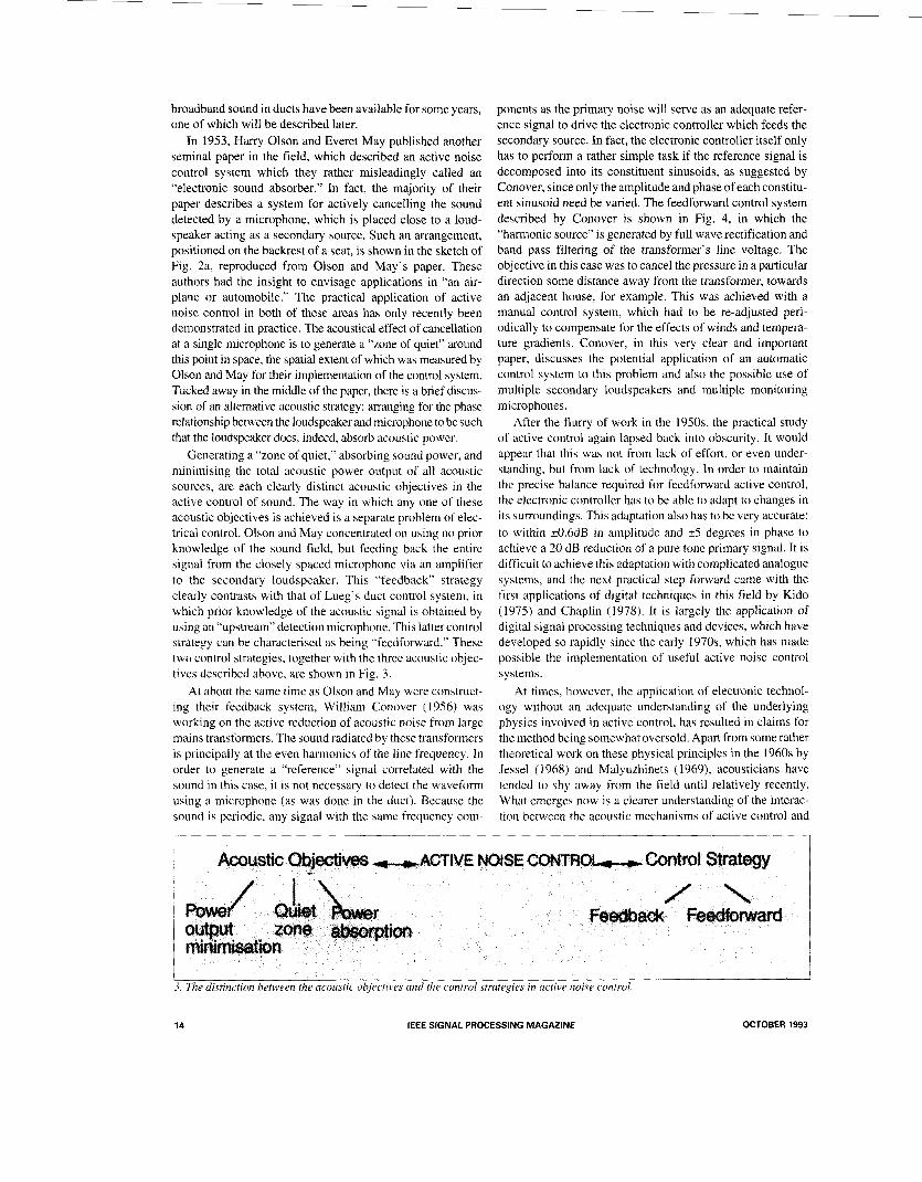
Generating a “zone of quiet,” absorbing sound power, and minimising the total acoustic power output of all acoustic sources, are each clearly distinct acoustic objectives in the active control of sound. The way in which any one of these acoustic objectives is achieved is a separate problem of electrical control. Olson and May concentrated on using no prior knowledge of the sound field, but feeding back the entire signal from the closely spaced microphone via an amplifier to the secondary loudspeaker. This “feedback” strategy clearly contrasts with that of Lueg’s duct control system, in which prior knowledge of the acoustic signal is obtained by using an “upstream” detection microphone. This latter control strategy can be characterised as being “feedfonvard.” These two control strategies, together with the three acoustic objectives described above, are shown in Fig. 3.

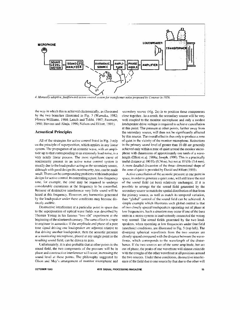
At about the same time as Olson and May were construct- ing their feedback system, William Conover ( 1956) was working on the active reduction of acoustic noise from large mains transformers. The sound radiated by these transformers is principally at the even harmonics of the line frequency. In order to generate a “reference” signal correlated with the sound in this case, it is not necessary to detect the waveform using a microphone (as was done in the duct). Because the sound is periodic. any signal with the same frequency com-

ponents as the primary noise will serve as an adequate reference signal to drive the electronic controller which feeds the secondary source. In fact, the electronic controller itself only has to perform a rather simple task if the reference signal is decomposed into its constituent sinusoids, as suggested by Conover, since only the amplitude and phase of each constituent sinusoid need be varied. The feedforward control system described by Conover is shown in Fig. 4, in which the “harmonic source” is generated by full wave rectification and band pass filtering of the transformer’s line voltage. The objective in this case was to cancel the pressure in a particular direction some distance away from the transformer, towards an adjacent house, for example. This was achieved with a manual control system, which had to be re-adjusted peri- odically to compensate for the effects of winds and tempera- ture gradients. Conover, in this very clear and important paper, discusses the potential application of an automatic control system to this problem and also the possible use of multiple secondary loudspeakers and multiple monitoring microphones.

After the flurry of work in the 1950s, the practical study of active control again lapsed back into obscurity. It would appear that this was not from lack of effort, or even understanding, but from lack of technology. In order to maintain the precise balance required for feedfonvard active control, the electronic controller has to be able to adapt to changes in its surroundings. This adaptation also has to be very accurate: to within +0.6dB in amplitude and +5 degrees in phase to achieve a 20 dB reduction of a pure tone primary signal. It is difficult to achieve this adaptation with complicated analogue systems, and the next practical step forward came with the first applications of digital techniques in this field by Kid0 (1975) and Chaplin (1978). It is largely the application of digital signal processing techniques and devices, which have developed so rapidly since the early 1970s, which has made possible the implementation of useful active noise control systems.

At times, however, the application of electronic technology without an adequate understanding of the underlying physics involved in active control, has resulted in claims for the method being somewhat oversold. Apart from some rather theoretical work on these physical principles in the 1960s by Jessel (1968) and Malyuzhinets (1969), acousticians have tended to shy away from the field until relatively recently. What emerges now is a clearer understanding of the interac- tion between the acoustic mechanisms of active control and

3. The distinction between the acoustic objectives and the control strategies in active noise control


LOUDSF€AKER MICROPHONE

4. Manually adaptive, feedforward active control system for transformer noise proposed by Conover in 1956.

the way in which this is achieved electronically, as illustrated by the two branches illustrated in Fig. 3 (Wamaka, 1982; Ffowcs-Williams, 1984; Leitch and Tokhi, 1987; Swanson, 1990; Stevens and Ahuja, 1990; Nelson and Elliott, 1991).

Acoustical Principles

All of the strategies for active control listed in Fig. 3 rely on the principle of superposition, which applies in any linear system. The propagation of an acoustic wave, with an amplitude up to that corresponding to an extremely loud noise, is a very nearly linear process. The most significant cause of nonlinearity present in an active noise control system is usually due to the loudspeaker acting as the secondary source, although with good design this nonlinearity, too, can be made small. There can be compounding problems with loudspeaker design for active control. In controlling a pure, low-frequency tone, for example, the cone may be required to undergo considerable excursions at the frequency to be controlled. Because of destructive interference very little sound will be heard at this frequency. However, any harmonics generated by the loudspeaker under these conditions may become dis- tinctly audible.

Destructive interference at a particular point in space due to the superposition of optical wave fields was described by Thomas Young in his famous “two slit” experiment at the beginning of the nineteenth century. The same effect is simple to engineer in acoustics: if the amplitude and phase of a pure tone signal driving one loudspeaker are adjusted relative to that driving another loudspeaker, then the acoustic pressure at a monitoring microphone, placed at any single point in the resulting sound field, can be driven to zero.

Unfortunately, it is also probable that at other points in the sound field, the two components of the pressure will be in phase and constructive interference will occur, increasing the sound level at these points. The philosophy suggested by Olson and May’s arrangement of monitor microphone and

secondary source (Fig. 2a) is to position these components close together. As a result, the secondary source will be very well coupled to the monitor microphone and only a modest loudspeaker drive voltage is required to achieve cancellation at this point. The pressure at other points, further away from the secondary source, will then not be significantly affected by this source. The overall effect is thus only to produce a zone of quiet in the vicinity of the monitor microphone. Reductions in the primary sound level of greater than 10 dB are generally achieved only within a zone of quiet around the monitor microphone with dimensions of approximately one tenth of a wavelength (Elliott et a], 1988a; Joseph, 1990). This is a practically useful distance at 100 Hz (0.34 m), but not at 10 kHz (3.4 mm). A more detailed discussion of the three- dimensional shape of the zone of quiet is provided by David and Elliott (1 993).

Active cancellation of the acoustic pressure at one point in space, in order to generate a quiet zone, will still leave the rest of the sound field (at best) relatively unchanged. If it is possible to arrange for the sound field generated by the secondary source to match the spatial distribution of that from the primary source, as well as match its temporal variation, then “global” control of the sound field can be achieved. A simple example which illustrates such global control is that of two closely spaced loudspeakers operating out of phase at low frequencies. Such a situation may occur if one of the bass units in a stereo system is inadvertently connected the wrong way around. The sound fields generated by the two loudspeakers, when operating at low frequencies under free field (anechoic) conditions, are illustrated in Fig. 5 (top left). The diverging spherical wavefronts from the two sources are closely spaced compared with the distance between the wavefronts, which corresponds to the wavelength of the disturbance. If the two sources are of the same amplitude, but are out of phase, the peaks of one wavefront will almost coincide with the troughs of the other wavefront at all positions around the two sources. Under these conditions, destructive interference of the field due to one source by that due to the other will


Separation of the two sources ( ).is the acoustic wavelength) 3 (c)

. The wavqfronts,froni prima? (blue) rind se~conclun (rerlj ~ ico i i~ t ic ~oiirc.es at,freyii~ncie.s where the source separation is ( a ) sinal1 mid (b ) Ieirge cornpared Lvith the acvustic ~cnve- length. WTD (dashed curve) is the \wricition ofthe net cicoustic p o ~ ~ r output of the ti1.o sources if the secondan ~oiirce i s ofthe sciine incignitue/e birr oiit ofphei . se with the primeivy source; W T ( ~ is the net povt3er outpiit when the ,sec~oridar~ ~ o ~ i r i ~ e ri~ngriitiitle cn7d phase ore optiinolly adjusted to miriimse the net power oiitput.

have been achieved globally. As the frequency of excitation is increased, the wavelength of the sound waves is reduced until it becomes comparable with the separation distance between the two sources (Fig. 5, top right). The distance between the two sets of wavefronts is then no longer small compared with the acoustic wavelength. Thus, the interference between the two sound fields will be destructive at some locations but constructive at others, and global control will not be achieved.

Another way of looking at this effect is to consider the total acoustic power output of the two sources. This analysis is presented in Design Guide 1 , and the dashed curve in Fig. 5 shows the change in the net acoustic power output of two equal but out-of-phase sources as their separation distance is increased compared with the acoustic wavelength (which is equivalent to raising the excitation frequency for a fixed separation). At large separation distances compared with the wavelength, the two sources radiate almost independently and generate a total power output which is twice that of either one operating alone, an increase of 3 dB in power output level. As the two sources are brought together, the interference becomes much stronger. and the total power output is significantly reduced compared with that of one source operating alone. A monopole source has then effectively been converted into a dipole source with a subsequent decrease in radiation efficiency.

I I t

-20 ' , '

What has been described above is not, however, true active control, since the amplitude and phase of one source was fixed apriori with respect to that of the other source. If total power output is taken to be the criterion which the active control system must minimise, the amplitude and phase of one source (the secondary) can be adjusted with respect to the other source (the primary) to achieve this objective for any given separation distance (Nelson et al., 1987a). The result of such a minimisation (see Design Guide 1 ) is that the optimal secondary source strength is very nearly equal and opposite to that of the primary sources for small separations, but the amplitude of the optimal secondary source gets progressively smaller as the separation becomes larger. Interestingly, the phase of the optimal secondary source remains either exactly out-of-phase or in- phase with the primary as the separation is increased. The total power output of the primary and optimally adjusted secondary source is shown as the solid curve in Fig. 5 for a range of source separations. For small separations, the result is almost indistin- guishable from a dipole, indicating that this is the optimal low frequency

OCTOBER 1993 16 IEEE SIGNAL PROCESSING MAGAZINE

Consider two point monopole sources operating at the same frequency o; a primary source, whose complex volume velocity, qp is fixed, and a secondary source, whose complex volume velocity, qs, can be adjusted to achieve active control. The complex acoustic pressures at the positions of the primary and secondary source can be written as

P p = z p p s p + Zp&s

where Zpp and Z,, are the acoustic “input” impedances seen by the two sources, and Zsp = Zps is the acoustic “transfer” impedance between the sources. The acoustic power outputs of the primary and secondary sources can also be written as

where the superscript * denotes complex conjugation, and Re@) denotes the real part of x. The total power output of the two acoustic sources can now be written, after some manipulation (Nelson et al., 1987a) as

in which Rss = Re(Zss), Rpp = Re(Zpp) and Rsp = Re(Zsp). The terms Iqp12Rp+2 and lqJ2R,,/2 are recognised as the power outputs of the primary and secondary sources if each were operating alone. The cross terms involving Rsp thus describe the influence of the secondary source on the power output of the primary source and allow it to achieve active control.

In the free field case, if the monopole sources are a distance r apart, then the real part of the radiation and transfer impedances are

“P p p 4m()

Rss=R =-

W2P Rsp = ---sinc kr 4nco

where sine kr is sin krkr, p is the density of the fluid, CO 2x h

its speed of sound, and k- the wavenumber, where h is

the acoustic wavelength.

Dipole Source If the secondary source strength is s

out of phase with, the primary source = qP (an obvious active control strateg equations above, the total power output in the free field can be shown to be

where Wpp = lqp12Rp@ is the power o source alone. Provided kr is less

a, that is, r > A, then the power output o will be approximately twice that of the alone.

Optimally Adjusted Secondary The total power output of the source p function of the real and imaginary al., 1987a) which has a minimum value o with a unique secondary source case, this optimum secondary so the solution of a set of equations form of the normal equations (Haykin, 1 case reduce to

qso = -RZ Rsp qp = -qp sine kr

so that thesecondar y source is alwaysei or in phase with the primary source an

Substitutingthis secon thegener alexpr ession for expression fort hemin imu

Wro = Wpp[ 1 - sinc2kr] which is equal to WTD for kr < 1, but never greater than Wpp. WTD and WTO Fig. 4.

Design Guide 1: Minimum Power Output of Two Monopole Sources

-


U 'rimary source

Secondary Electrical Monitor source filter microphone

7. ( a ) Active noise system (block diagram) usingjeedback control. (b) Eyuivulent electrical configuration. ( c ) Block diagram of digital controller. ( d ) Equivalent block diagram ifk(:) = C(z).

strategy. For larger source separations, the total power output of the primary and optimally adjusted secondary is never greater than that of the primary source alone. This is to be expected since, at the very least, the secondary source can act to not increase the net power output by reducing its strength to zero, as indeed it does at large source separations.

If the source separation is small and the total power output of the source pair is very much less than that of the primary source alone, the naive observer sometimes raises the ques- tion of "where does the power go?'The acoustic power output of each source can be calculated when the secondary source is adjusted to minimise total power output, and it is found that the acoustic power output of the secondary source under these conditions is exactly zero (Nelson and Elliott, 1987). It is thus neither radiating nor absorbing sound power. The power output of the primary source is thus necessarily reduced by this control strategy. The action of the secondary source is to decrease the net acoustic radiation resistance seen by the primary source by reducing, as best it can, the acoustic pressure at the position of the primary source which is in- phase with its volume velocity.

An entirely different strategy of active control emerges if instead of minimising the total power output of the source pair, the acoustic power absorption of the secondary source is maximised (Nelson et al., 1988b; Elliott et al., 1991). This is clearly not the mechanism of control described previously, where the total power output is minimised), since the power output of the secondary source under such conditions is always zero (Elliott et al., 1991). If the amplitude and phase of the secondary source are adjusted so that it is maximally absorbing sound power, then for small source separations the

secondary source strength becomes much larger than that of the primary source, and in quadrature with it. This effect causes a substantial increase in the net radiation resistance experienced by the primary source and a subsequent large increase in its power output. Approximately half the power now radiated by the primary source is absorbed by the secondary source, and the other half is radiated into space, considerably increasing the total power output of the source pair. Power absorption, using a closely coupled source, thus does not appear to be an efficient strategy for global control!

Sound in Enclosures

In the previous description, it was shown that global control of the sound field due to a closely spaced pair of free field sources can be obtained by minimising their net acoustic power output. In an enclosure such as the interior of a car or an aircraft, the sound field is not freely propagating but reflected off the enclosure boundaries, causing internal standing waves at certain frequencies. These three-dimensional standing waves are the acoustic modes of the enclosure and an efficient way of describing the acoustic pressure in an enclosure at low frequencies in terms of the sum of the contributions from each of these modes.

The global effect of an active noise control system in an enclosure can be assessed using the total acoustic potential energy in the enclosure (Nelson et al, 1987b). This quantity is proportional to the sum of the mean square amplitudes of each of the acoustic modes. Given the position of a pure tone primary source in the enclosure and that of a controllable secondary source, an optimisation similar to that presented in

IEEE SIGNAL PROCESSING MAGAZINE OCTOBER 1993 18

Design Guide I , can be performed to minimise the total acoustic potential energy by adjusting the amplitude and phase of the secondary source. It tums out that the total acoustic potential energy is very nearly proportional to the net acoustic power output of the two sources inside the enclosure, and minimising the total acoustic potential energy is almost equivalent to minimising the net power output (Elliott et al., 1991).

The total acoustic potential energy generated in a rectan- gular enclosure of dimensions 1.9m x 1. l m x 1 .Om (roughly equivalent to the interior of a small car), by a pure tone monopole acoustic source in one comer of the enclosure is shown in Fig. 6, for a range of excitation frequencies. The natural frequencies and the shapes of some of the acoustic modes which occur in this enclosure over the frequency range considered are also shown, and the resonant increases in energy near the natural frequencies of the acoustic modes are clearly seen. The heights of these peaks are determined by the amount of acoustic absorption within the enclosure. In Fig. 6, the assumed acoustic absorption is about one tenth that actually measured inside a car, so the peaks are somewhat larger than they would be in practice. Also note the way the modes tend to clump together, in the region of 175 Hz for example, due to the fact that the enclosure is about twice as long as it is broad and high.

A secondary acoustic source is now introduced in the opposite comer of the enclosure and driven at the same discrete frequency as the primary source. Its amplitude and phase are adjusted to minimise the total acoustic potential energy in the enclosure, and the resultant total acoustic potential energy is plotted as the dashed curve in Fig. 6. At excitation frequencies where only a single acoustic mode dominates the response of the enclosure (below 30 Hz and close to 90 Hz, for example), very large reductions in energy can be achieved with this single secondary source, since it can drive the dominant acoustic mode to an equal and opposite extent as does the primary source. For excitation frequencies between the natural frequencies of the low frequency modes, however, or at most frequencies above 200 Hz, many acoustic modes contribute to the response in the enclosure. The secondary source is unable to control any one of these acoustic modes without increasing the excitation of a number of other modes, and so the optimum secondary source strength is reduced in these frequency regions and little reduction in the total acoustic potential energy is achieved.

Increasing the number of secondary sources would increase the number of acoustic modes which could be actively controlled. Unfortunately, the number of significantly con- tributing acoustic modes in an enclosure (which is proportional to the acoustic “modal overlap”) increases at higher frequencies in approximate proportion to the cube of the excitation frequency. As a consequence, doubling the number of secondary sources by no means doubles the upper frequency limit of control. An upper frequency limit of perhaps a few hundred hertz is thus imposed on a global active noise control system, in an enclosure of dimensions discussed above, because of the fundamental acoustic properties of the

enclosure. It may still be possible, however, to actively control the sound in an enclosure to some extent at these high frequencies, by arranging for loudspeakers on the boundaries of the enclosure to absorb acoustic energy and thus increase the average absorption coefficient in the enclosure (Guicking et at, 1985).

In practice, it is not possible to measure the total acoustic potential energy in an enclosure, since such a measurement would require an infinite number of microphones distributed throughout the enclosure. If, however, the sum of the squares of a finite number of microphones is used as the criterion which the active control system minimises, reductions in the total acoustic potential energy very nearly as large as those presented in Fig. 6 can be obtained with relatively modest numbers of microphones. The microphones need to be positioned in the enclosure such that they are affected by all the dominant acoustic modes, in the same way that the secondary sources need to be positioned such that they can excite these modes. It has been found in practice that having approximately twice as many sensibly positioned microphones as secondary sources provides a reasonable compromise between complexity and performance.

Feedback Control

The feedback control approach, as applied in active noise control, was described above in relation to Olson and May’s arrangement (Fig. 2b). A more idealised physical illustration of such a system and its equivalent electrical block diagram is shown in Fig. 7. In this figure, e represents the signal derived from the microphone, due to the combined effect of the primary disturbance, d, and the feedback loop. The electrical transfer function of the feedback loop, H , was a simple gain and phase inversion described by Olson and May. The electrical transfer function from secondary loudspeaker input to microphone output, C, is called the secondary or error path. This system corresponds to the “plant” in conventional feedback control. In this case, it contains the electroacoustic response of the loudspeaker, the acoustic characteristics of the path between loudspeaker and microphone, and the microphone’s electroacoustic response. The transfer function between the disturbance and measured error is thus

E(s) 1 D(s) - 1-C(s)H(s)

If the frequency response of the secondary path, C(jo ), were relatively flat and free from phase shift, then the gain of an inverting amplifier in the feedback path, H( jo )=-A, could be increased without limit, causing the overall transfer function of the feedback loop to become arbitrarily small. This is analogous to the virtual earth concept used in operational amplifiers and such a control system is sometimes referred to as an “acoustic virtual earth.” The effect of the feedback loop forcing e to be small compared to d, will be to cancel the acoustic pressure at the monitor microphone, as required for active control.


Unfortunately, the frequency response of the secondary path, C ( j w ) , can never be made perfectly flat and free of phase shift. The electroacoustic response of a moving coil loudspeaker, in particular, induces considerable phase shift near its mechanical resonance frequency. The acoustic path from loudspeaker to microphone will also inevitably involve some delay due to the acoustic propagation time, and this will also introduce an increasing phase shift in the secondary path with increasing frequency. As the phase shift in the secondary path approaches 180” the negative feedback described above becomes positive feedback and the control system can become unstable. Fortunately, as the frequency rises and the phase lag in the secondary path increases, its gain also tends to decrease. It is thus still possible to use an inverting amplifier in the electrical path provided its gain is not large enough to make the net loop gain greater than unity when the total phase shift becomes 180”. This stability criterion can be more formally described using the well-known Nyquist criterion. At lower frequencies the feedback will be negative and the loop gain may still be considerably greater than unity, thus ensuring that some attenuation of the signal from the microphone is produced.

It is possible to introduce compensating filters into the electrical path to correct for the phase shift in the secondary path to some extent, and increase the bandwidth over which active control is possible. First and second order lead-lag networks, for example, have been successfully used in practice by Wheeler (1986) and Carme (1987). It is not, however, possible to design a compensation filter which will minimise the mean square value of the error signal, e, under all circum- stances. This is because the spectrum of the primary noise disturbance, d, can change considerably over time, and a compensation filter designed to produce good attenuation in one frequency band will not necessarily produce as good an attenuation in another frequency band. For this reason, some authors have suggested that different compensation filters be used in feedback control systems designed for differing noise environments (Veight, 1988).

The optimum design of a feedback controller can be for- mulated in terms of the state space models which are often used in conventional control theory (see for example Good- win and Sin, 1984; Wellstead and Zarrop, 199 1 ). The problem can also be viewed from a signal processing viewpoint (El- liott, 1993), which gives some insight into the performance limitations of feedback control, and also suggests how the feedback controller could be implemented using adaptive digital filters. If the controller is digital, i.e., it operates on sampled data, the general block diagram can still be represented as in Fig. 7b, except that the sampled transfer function of the system under control, C(z), now contains the responses of the data converters and any anti aliasing or reconstruction filters used. In general, C(z) will not be minimum phase and may contain some bulk delay. We now assume that the controller is implemented as the parallel combination of a “feedback’ path, W(& and a “feedforward” path, &), as shown in Fig. 7(c). The transfer function of the controller is thus

r L - - - - - - - - - - L

Primary Electrical Secondary Monitor source filter source microphone

. ( a ) Active noise system (block diagram) using feedforward con. trol. (b) Equivalent electrical conjiguration.

Such a controller arrangement is similar to the echo cancellation architecture used in telecommunications Sondhi and Berkley, 1980; Adams, 1985), and the feedback cancellation architecture used for feedforward controllers (as described below). Its use in feedback control has been suggested by Forsythe et al. (1991). With such a controller the response of the complete feedback control system becomes

Clearly, if the “feedforward” part of the controller is adapted to have the same transfer function as the system under control so that &(z)=C(z), then the error signal becomes

The block diagram representing this equation is shown in Fig. 7d, which follows from Fig. 7c if it is noted that when &(z)=C(z), then the signal driving W(z), x(n), becomes equal to the disturbance d(n).

The feedback control problem has thus been transformed into an entirely feedforward problem. In the special case of the plant response C(Z) corresponding to a pure delay, Fig. 7d is the block diagram of an adaptive line enhancer (Widrow and Steams, 1985). To minimise the mean square value of the


error, W(z) must act as an optimal predictor for the disturbance signal. In general, the performance of the feedback controller will depend on the predictability of the disturbance signal filtered by the plant response. This action is similar to the prediction achieved in minimum variance controllers (Good- win and Sin, 1984). In practice the two parts of the controller, W(z) and &z), could be implemented by adaptive digital filters. For example, before control, &(z) could initially be adapted to model C(i) by using a broadband identification signal added to the plant input u(n) and adapting k(z) using the LMS algorithm to minimise x(n). W(z) could then be adapted using the filtered-x LMS algorithm with a copy of k ( z ) to generate the filtered reference signal as described below. It may also be possible to simultaneously adapt the two parts of the filter. Alternatively, it may be possible to use the RLMS algorithm to adjust both filters, in a similar way to that described by Billout et al. (1 991). The feedback control architecture illustrated in Fig. 7c can be readily extended to plants with multiple inputs and multiple outputs. The practi- cality of such an architecture for a feedback controller remains to be investigated in detail, but such an arrangement has been successfully used by Stothers et al. (1993) to design the controller for a feedback control system to suppress sun roof flow oscillations in cars. The consequences of this model of the controller provide an interesting signal proessing insight into the behaviour of a feedback controller, and the reasons why the optimal feedback controller depends upon the statis- tical properties of the primary disturbance, d(n), and the plant response C(z).

Active control systems using feedback have been used to control the noise propagating in ducts, in which case the secondary loudspeaker is positioned on the side of the duct and the monitor microphone is placed adjacent to this (Eghte- sadi and Leventhall, 1981; Trinder and Nelson, 1983). The most successful application of feedback systems in active control, however, has been for broadband noise control in closed and open-backed headsets and ear defenders. Several commercial systems are now available which achieve 10- 15 dB reductions in pressure from very low frequencies (about 30 Hz) up to about 500 Hz. Even though the monitor microphone can be placed very close to the secondary source in these applications, the high frequency limit is still set by the inevitable accumulation of phase shift with frequency, causing instability unless the gain is reduced. Another problem which practical active headset systems have to contend with is the variability of the secondary path while in use. This is because of the changeability of the acoustic path between secondary loudspeaker and monitor microphone as the headset is worn by different people, or in different positions by the same person, or even as it is lifted on and off the head. Careful design of the compensation filter can be used to ensure that the active headset is reasonably robust to such variability. A similar problem also occurs in the arrangement described by Olson and May (Fig. 2a) because the frequency response of the secondary path is significantly altered as the listener changes the position of his head.

I

1 W C x(nJ

I

?

w(n+l) = w(n) - a r (n) e(n)

. ( a ) Elecrrical noise canceller (block diagram) using ?he LMS algorithm. (b) Active noise control system adapted using the “filtered-x LMS” algoritlzm. (c ) Equivalent active noise control sys- ten1 for quasi-static adaptation.

There is another advantage to using an active control system when the headset is also used to reproduce a communications or music signal. If the communications signal is electrically subtracted from the output of the monitor microphone, the pressure at the microphone position will be regulated by the action of the control system to faithfully follow the communications signal. The overall transfer function from communications signal to acoustic pressure is i n this case proportional to -C(s)H(s) / [ 1 -C(s)H(s)]. If the loop gain is large and negative (i.e., -C(s)H(s) > I ) as required for active control, then the reproduction of the communications signal will be essentially independent of the response of the loudspeaker and acoustic response of the headset, C(s), and a more faithful reproduction of the communications signal will be achieved.

Feedforward Control

Feedforward methods of active noise control have been illustrated for broadband noise in ducts (Fig. 1 ) and for pure tone noise generated by transformers (Fig. 2). A generic block diagram for such systems is shown in Figure 8a. The differ-


ence between this and the feedback approach is that a separate reference signal, x, is now used to drive the secondary source, via the electrical controller, W. This reference signal must be well correlated with the signal from the primary source. In systems for the control of broadband random noise, the reference signal provides advance information about the primary noise before it reaches the monitor microphone, which en- ables a causal controller to effect cancellation. In systems for the control of noise with a deterministic waveform, such as harmonic tones, this “advanced” information has little mean- ing since the controller only has to implement the appropriate gain and phase shift characteristics at each frequency.

Another difference between the broadband and harmonic controllers is that in the latter case an electrical reference signal can often be obtained directly from the mechanical operation of the primary source, using a tachometer signal from a reciprocating engine for example. Such a reference signal is completely unaffected by the action of the secondary source and the control is purely feedforward, as illustrated in Fig. 8. In the broadband case, such as random noise propagating in a duct, a detection microphone often has to be used “upstream” of the secondary source to provide the reference signal, A4 (diagram 1 of Fig. 1). In this case, the output of the detection microphone, as well as being influenced by the primary source, will also be affected by the operation of the secondary source. A potentially destabilising feedback path will thus exist from the secondary source to the detection sensor. The simplest method of removing the effects of this feedback path, before feedforward control is attempted, is to use an electrical model of the feedback path within the controller, which is driven by the signal fed to the secondary source and whose output is subtracted from the output of the detection sensor. Such an approach is analogous to the echo cancellation techniques used in telecommunications systems (Sondhi and Berkley, 1980).

The electrical block diagram of the purely feedforward controller is shown in Fig. 8b. We denote the frequency response of the secondary path from secondary source input to monitor microphone output as C(jw), the frequency response of the controller as W(jw), and the frequency response of the primary path from reference signal to monitor microphone as P(jo) . The spectrum of the error signal EUo) compared with that of the disturbance, DUO), is thus

_ _ _ _ Eo“) - + ~tiwm) Do”) Po’@))

Because the spectrum of the error signal is linearly related to the response of the electrical controller, WOO), this can, in principle, be adjusted at each frequency to model the response of the primary path, P(jo). and invert the response of the secondary path, C(jo) , and thus give complete cancellation of the error spectrum. The frequency response required of the controller in this idealised case is thus W(j~)=-P(jw)/Cfjo) , and for pure tone disturbances this equation only has to be true at a single frequency for active control to be accurately implemented. In the broadband case the problem becomes

one of practical filter design. so that the coefficients of the electrical filter used in the controller are designed to give a frequency response which best approximates the one required. Another complication in the broadband case is that often measurement noise is present in the reference signal due, for example, to the air flow over the microphone in a duct. The frequency response of the controller which best minimises the power spectral density of the error signal in this case is a compromise between cancellation of the primary noise signal and amplification of the measurement noise through the controller (Roure, 1985).

Because the properties of the primary noise and, to a lesser extent, the characteristics of the secondary path will probably change with time in a practical system, the controller in active feedforward systems is often made adaptive. The most convenient method of implementing an adaptive filter is using digital techniques and it is the application of such adaptive filters to feedforward active control which is currently one of the most interesting applications of signal processing in active noise control.

Adaptive Filters in Single Channel Control Systems

There are significant differences between a conventional, electrical noise canceller (Fig. 9a) and a single channel active noise control system (Fig. 9b). The well-known LMS algorithm is widely used for electrical noise cancellation (Widrow and Stearns, 1985). If this algorithm is used without modifi- cation in an active control application, however, the result is likely to be an unstable system. This is because the signal from the adaptive filter, W, suffers a phase shift in passing through the secondary path, C. The instantaneous measurement of the gradient of the mean square error with respect to the coefficient vector, x(n)e(n), is thus no longer an unbiased estimate of the true gradient. The solution to this problem, first proposed by Morgan in 1980 and independently by Widrow et ul., and Burgess in 1981, is to introduce a similar phase shift into the reference signal path, before the gradient estimate is formed. This is achieved by using an electrical filter, e, which models the response of the secondary path C, to generate a filtered reference signal, r(n). The reference signal is then multiplied by the error to form the gradient estimate. The resulting update equation is called the “filtered- x LMS” algorithm.

Another way ofjustifying this algorithm is to consider the case in which k=C and the control filter, W, is changing only slowly with time. Under these conditions, the order of the operations on the reference signal can be commuted and an almost equivalent output would be produced by passing the reference signal first through the secondary path, C, and then through the filter W (Fig. 9c). Since the direct output of the control filter would now be observed at the error signal, the normal LMS algorithm could be used, although the relevant reference signal would be that filtered by C. In practice, the filtered-x LMS algorithm is stable even if the control filter coefficients do change significantly in the timescale associ-


Consider the problem of adjusting the coefficients of an array of FIR control filters in the multichannel case. K reference signals, xk(n), are available. These are fed to a matrix of FIR control filters, whose outputs are used to driveM secondary sources, with outputs signals ym(n). The m k-th filter, which is assumed time invariant for the time being, has coefficients, w,ki, so that

Each control filter output is linearly coupled to each of L error sensors, with outputs ei(n), via secondary paths which can be modelled as (fixed) J-th order FIR filters (where J can be as large as necessary), so that

and where clmj are the coefficients of the Im-th filter and dl(n) is the output of the I-th error sensor in the absence of control, i.e., due to the primary field. Substituting the equation for ym(n) above into that for el(n) gives

which may be rewritten as a single summation over the number of control filter coefficients (MKI) as

where is the k-th reference signal filtered by the response of the path from the m-th secondary source to the l-th error sensor:

Design Guide 2: The Multiple Error LMS Algorithm

-

ated with the dynamic response of the secondary path. The maximum convergence coefficient which can be used in the filtered-x LMS algorithm has been empirically found (Elliott et al., 1989) to be approximately

- where -r2 is the mean square value of the filtered reference signal, I is the number of filter coefficients, and 6is the overall delay in the secondary path (in samples). This compares with the limit for the normal LMS algorithm, which is approximately (Widrow and Stems, 1985)

We now seek the stochastic gradient algorithm whic adjusts all the control filter coefficients to minimise th instantaneous cost function equal to the sum of the square signals at the error sensors:

L

z= 1

The derivative of J(n) with respect to the general contrc filter coefficient wmki, is

where the final expression follows from the equation fc el(n) above. Updating each filter coefficient by an amoui proportional to - dJ(n) / dwmki at every sample time leac to a simple form of the Multiple Error LMS algorithi (Elliott and Nelson, 1985):

L

1=1

where a is a convergence coefficient. The success of the control algorithm depends on a

number of factors including whether (a) The reference signals persistently excite the control filters so that ill-conditioning is avoided; (b) the FIR model of each secondary path can be accurately measured so that the true filtered reference signals can be generated; (c) the speed of adaptation of the control filter coefficients is sufficiently slow so as not to invalidate the assumption that the control filters are time invariant.

The delay in the secondary path, which usually forms the most significant part of the dynamic response of this system, thus reduces the maximum convergence coefficient in the filtered-x algorithm, but only to the extent that the speed of response is comparable with the delay, 6. In actively controlling the sound in an enclosure with dimensions of a few metres, this delay is typically of the order of 10 ms and initial convergence speed is fairly rapid. The LMS algorithms can exhibit other, slower, modes of convergence whose time constants are determined by the eigenvalues of the reference


K M L reference secondary Disturbance

sources se(ls0rs A

S I N S

K df (LxM) matrices of filters mcdling e m

Dams

(KMlXl) ( K M I X L ) (kl) composite filtered ermr COeRiaent reference agnal

vectw ~(onalmalnx W o r

3. General multichannel active noise control system, adapted ing the “Multiple Error LMS” algorithm.

signal autocorrelation matrix E[x(n)xT(n)]. Similar slow modes are observed for the filter ed-x LMS algor it hm due to the eigenvalue spread of the autocorrelation matrix of the filter edr efer encesignal,E[ r(n)rT(n)]. This behaviour can be understood by considering the action of the filtered-x algorithm in terms of the almost equivalent representation of Fig. 9c, in which a normal LMS algorithm is used with a modified reference input.

The stability of the filtered-x LMS algorithm is also affected by the accuracy of the filter (A modeling the true secondary path (c). The estimate of the gradient vector does not have to be exact, however, and the filtered-x algorithm is surprisingly robust to errors in &. Morgan (1980) has shown that for pure tone reference signals the phase of at the excitation frequency only has to be within f90 degrees of e that of the true error path, C, for the system to converge slowly. Numerical results (Boucher et al., 1991) also suggest that phase errors of 40 degrees hardly affect the maximum convergence speed of the algorithm. Similarly, Widrow and Stearns (1985, p. 292) remark, in the context of using the filtered-x LMS algorithm for adaptive inverse control, that this model “need not be very precise,” and that its most important attribute is that “its impulse response has at least as great a transport delay” as the secondary path.

The implementation of the filtered-x LMS algorithm is somewhat more complicated than that of the normal LMS, because of the need to generate the filtered reference signal. The filter used to model the secondary path is often created in an identification phase, prior to control, during which a training signal is fed to the secondary source. This filter could be another FIR filter which is adjusted, during identification, using a separate LMS algorithm. Because the response of this filter does not have to exactly match that of the secondary path, it is often only necessary to use relatively few coefficients in this filter.

Control filter structures other than the FIR one discused above, have also been used in active control applications. In particular, Eriksson and his colleagues have developed an adaptive recursive controller (Eriksson et al., 1987). A recursive filter has the ability to accurately model the response required for active noise control in a duct, without the need

for explicit feedback cancellation. These authors have also discussed the effect of continuously identifying the secondary path at the same time as implementing active control, together with the other practical problems which occur when an active control system is implemented in an industrial environment (Eriksson and Allie, 1989). Some initial studies using lattice filters in active noise control systems have also been reported (Sudararajan et a], 1985; Mackenzie and Hansen, 1991; Swanson, 1991).

Adaptive Filters in Multiple Channel Control Systems

When the single channel active control systems described above is used to control a deterministic primary waveform, the signal from the single monitor microphone can be driven to zero. A single channel controller could be used, for example, to produce a zone of quiet around the monitor microphone using a closely spaced secondary source, as discussed earlier. If, however, such a system were used in an attempt to achieve global active control in an enclosure by placing the microphone some distance away from the secondary source, the result might well not be satisfactory. An unacceptable result would certainly be obtained if, due to its positioning in the enclosure, the secondary source was only weakly coupled to the monitor microphone at the excitation frequency. The secondary loudspeaker would thus have to drive very hard to cancel the primary field at the microphone, and although a small zone of quiet would be generated at this point, the sound pressure at other points in the enclosure would tend to rise significantly.

Clearly what is required is a practical measurement which gives a better estimate of the acoustic quantity which it is desired to control with a global system: the total acoustic potential energy. This quantity is proportional to the volume integral of the mean square acoustic pressure throughout the enclosure. A single pressure measurement is obviously a poor estimate of this volume integral if the driving frequency is high enough for a number of acoustic modes to be significantly excited. A better estimate of the volume integral would be the sum of the mean square pressures at a number of locations throughout the enclosure volume.

This practical requirement motivates the development of a generalisation of the filtered-x LMS algorithm in which the filter coefficients are adjusted to minimise the sum of the mean square values of multiple error signals. In fact, further generalisation is then possible to include the practically important cases of multiple secondary sources, and its use with multiple reference signals. The resulting “Multiple Error LMS” algorithm (Elliott and Nelson, 1985) is described in Design Guide 2 . Each coefficient of the adaptive filter driving each secondary source from each reference signal is now adjusted every sample by an update term composed of the sum of the products of each error signal with the corresponding filtered reference signal.

Figure 10 shows the block diagram of an active control system with K reference signals, M secondary sources and L


~ ~~ ~~~~~~ ~

Design Guide 3: A Generalised Multiple Error Algorithm

Consider the minimisation of a more general cost function than that discussed in Design Guide 2, in which all sampled signals are taken to be complex, and so could represent transformed variables. It is convenient to express the equations for the control filter outputs and error sensor outputs, derived above, in matrix form (Elliott et al., 1987, 1988) such that

Y (n) = X ( 4 w

where the vector of control filter outputs is y (n) = bi(n), y2(n) ... y k n ) ] ? w is the MKI x 1 vector containing the control filter coefficients, and X ( n ) is an M x MKI matrix of reference signals. Similarly, we can write

e(n) =d(n) +R(n)w

where the vector of error signals is e(n) = [e l@) , q ( n ) ... e,-(n)]T, d(n) is e(n) prior to control, and R(n) is a matrix of reference signals filtered by the true secondary paths. We now define a generalised cost function, similar to that used in optimal feedback control theory which includes both error and "effort" terms, as

J = E [eH(n> o e(n> +yH(n) Q, y(n)l

in which the superscript H denotes the Hermitian (complex conjugate transpose), and E denotes an expectation opera- tor. 0 is an error weighting matrix, which is Hermitian and positive definite but not necessarily diagonal, and Q, is an effort weighting matrix which is also Hermitian and positive definite but not necessarily diagonal. Using the equations for e(n) and y(n) above, this cost function can be expressed in the complex quadratic form

J = wHA w + wHb + bHw + c

in which

A = E [ p ( n ) O R(n) + f l ( n ) @ X(n)]

b = E [ p ( n ) O d(n)]

c = E [dH(n)O d(n)]

This equation has a unique global minimum, assuming A is positive definite, for a set of control filter coefficients given by

wept = -A-'b = -E [fl(n)O R(n) + f l ( n ) @ X(n) I-' E [& d(n) ]

which result in the least squares value of the cost function

Jmin = c -bHA-'b

The vector of derivatives of the real and imaginary components of the vector of control filter coefficients, W R and wi, can be written as (Haykin, 1986; Nelson and Elliott, 1991):

aJ aJ g = - + - = 2 [A w + b ] awR aw,

which in this case can be written as

g = 2E [ p ( n ) 0 e(n) + S ( n ) Q,y(n)]

In practice, only an approximation to each of the paths from secondary source to error sensor can be measured and used to generate the practically implemented filtered reference signals, the matrix of which is &n). Using the instantaneous estimate of g, with &n), to update all the control filter coefficients at every sample, yields the generalised version of the multiple error LMS algorithm in matrix form:

A convergence analysis of this algorithm can be performed in a similar manner to that generally used for the LMS algorithm (Widrow and Steams, 1985). The algorithm, if stable, converges to the solution which can be found by setting to zero the term in square brackets in the equation above, to give

wm = -E [ &n) 0 R(n) + Y ( n ) X(n) I-' E [ p ( n ) 0 d(n) 3

which is not, in general, equal to the optimal solution, wept above, since &n) #R(n). Using this expression for w -, substituting for e(n)=d(n)+R(n)w(n), and making the usual assumption that the variations in the filter weight vector are statistically independent of those of the reference signals, the update equation can be written as

E [w(n+l) - Wm ]

= [ I - aE [a"(n) 0 R(n) +X"(n ) @ X(n) 3 1 E [w(n) - Wm 1

the convergence of which depends on whether the real parts of the eigenvalues of the generalised autocorrelation matrix, E [ [ E ( n ) 0 R(n) +A? Q, X(n)], are positive. Note

that the eigenvalues of p ( n ) 0 R(n) are, in general, complex since&) is not necessarily equal toR(n), and the real parts of these eigenvalues are not guaranteed positive (as they would be in the normal LMS analysis) for the same reason. The effort term in this expression, F ( n > Q, ~ ( n ) , is guaranteed to be positive definite, however (assuming the control filters are persistently excited), and thus will have positive real eigenvalues which can have the effect of stabilising an otherwise unstable system (Elliott et al., 1992). Assuming the system is stable, the speed of convergence of the "modes" of the active control system are determined by the magnitudes of the real parts of the eigenvalues of the generalised autocorrelation matrix.


monitor microphones, which uses the Multiple Error LMS algorithm. There are now M x L different acoustic paths between each secondary source and each monitor microphone, each of which has to be modelled and used K times to generate the array of filtered reference signals required for the adaptive algorithm. This algorithm adjusts each of the coefficients of each of the K x M adaptive filters in the controller, which drive every secondary source from every reference signal. Although every stage in the implementation of the single channel filtered-x LMS algorithm is now replicated many times, the same basic elements (of secondary path model estimation, filtered reference generation and multiplication of error signals with these delayed filtered reference signals) are present in the multiple channel algorithm.

In fact, the implementation of quite large systems is often not as difficult as it would first appear, principally because the low frequency sound fields which one often wants to control in practice are periodic. Examples of such periodic sound fields which have been controlled in practice are the engine firing noise inside cars and the blade-passing noise due to the propellers inside aircraft, as will be discussed in more detail below. For example, a practical active control aystem built in 1987 for investigating the active control of propeller noise in a 50 seat aircraft (Elliott et al., 1990) had three reference signals ( K = 3) at the fundamental blade-passing frequency and its first two harmonics; sixteen secondary sources ( M = 16); and thirty two monitor microphones ( L =

1. ( a ) Physical implementation of an active control system w.ith a synchronously sampled reference signal, udupteil using the “filtered-x LMS” algorithm. (b) The equirdent Iineur transfer function, G, ofthe algorithm between error signal uiidfilter- input. ( c ) Frequency response of the complete closed loop transfer function from primarl): signal DGo) to residual error signol, E(@).

32). However, the computational burden of implementing the Multiple Error LMS algorithm at a sample rate of about 700 Hz was not excessive. This is because each of the reference signals was a sinusoid and so only two coefficients were required for each of the K x M = 48 individual control filters and K x M x L = 1536 individual filters used to generate each of the filtered reference signals. In fact, an array of 16 DSP chips (TMS 320C20) were used to implement the algorithm (one for each secondary source). A number of other monitoring functions were also implemented, however, and the proc- essors were not working at their full capacity.

In practical systems for the active control of engine noise in cars, the problem is further reduced since the enclosed volume is much less than that of a 50 seat aircraft. Typically, 2 loudspeaker-4 microphone or 4 loudspeaker-8 microphone control systems can be used to control up to 3 harmonics. In this application, however, the control filters must adapt to changes in excitation, due to changing engine speed and load for example, which occur on a much shorter timescale than those occurring during steady cruise in an aircraft. Practical implementations of the Multiple Error LMS algorithm used to control the engine noise in cars have a convergence time of the order of one tenth of a second. This rapid adaptation is important subjectively, so that the control system is not heard to lag behind the noise from the engine during gear changing, for example.

An automotive application which presents a greater chal- lenge than controlling engine noise, in terms of both design- ing and implementing a practical control system, is the active control of low frequency road noise (Sutton et al., 1989). An important distinction between this case and that of engine noise control is that the multiple reference signals which must be used have a random rather than a sinusoidal waveform. This means that the control filters, and those used to generate the filtered reference signals, must model a broadband response, and so have many more than two coefficients. This considerably increases the convergence time of the algorithm and the computational burden. Experimental systems to actively control road noise in cars have, however, been successfully demonstrated (McDonald et al., 1991).

The theoretical analysis of the behaviour of the Multiple Error LMS algorithm is not well developed. It is, however, possible to analyse some aspects of the convergence of the algorithm using similar methods to those used by Widrow, for example. in the analysis of the LMS algorithm (see Design Guide 3). This demonstrates that the convergence time of the different modes of convergence are dependent on the eigenvalues of a generalised autocorrelation matrix, whose eigenvalues depend not only on the spectral properties of the filtered reference signal but also on the spatial distribution of the microphones and loudspeakers. It also demonstrates that the system may be unstable, even for very small convergence coefficients, because of errors in the models of the secondary paths used to generate the filtered reference signals. For the particular case of a harmonic reference signal both these limitations can be more clearly demonstrated in a frequency domain analysis (Elliott et al. 1987, 1992; Boucher et al.,


1991). One important feature which comes out of such an analysis is the important stabilising influence of having a small “effort” term in the cost function being minimised. Such a term penalises large outputs of the secondary sources if they only produce small decreases in the signals from the monitor microphones (Elliott et al., 1992). It is found that small effort terms in the cost function also considerably reduce the risk of instability because of errors in the secondary path models (Boucher et al., 1991). The effect of effort weighting is very similar to that of having a “leak” in the update algorithm, so that the coefficients would slowly die away if the errors were to go to zero (Elliott etal . , 1987). Widrow and Stearns (1985) show that the presence of low level uncorrelated noise in the reference signal of an adaptive filter is also equivalent to having a leak in the LMS algorithm.

Because the reference signals in many practical active noise control systems are generated from a measurement sensor such as a microphone in a duct, which inevitably is corrupted by some measurement noise, a certain level of “natural” effort weighting is bound to be present. The stabilising influence of this otherwise unwanted noise signal may well have preserved the stability of many practical implementations of active control systems. In general, however, it is unwise to rely on such poorly controllable effects to provide stability, and an explicit effort term or leak in the algorithm is preferred.

Another potentially destabilising influence which is not taken into account in either the frequency domain analysis (Elliott et al., 1992), or in the time domain analysis outlined in Design Guide 3, is that of delays in the secondary paths. The reason why such delays are not accounted for is that both formulations inherently assume that the controller is adapting slowly and thus steady state conditions are preserved in the response of the secondary paths. The effect of delays in the secondary paths have been accounted for in a time domain analysis by Snyder and Hansen (1992). Another interesting way of analysing active control systems with deterministic reference signals which does take these dynamic effects into account, and demonstrates an interesting link between adaptive feedforward and fixed feedback control systems is outlined in the next section.

Equivalent Linear System Approach

In an important paper published by Glover in 1977, the “non-Wiener’’ behaviour of electrical noise cancelling systems with sinusoidal reference signals was examined. In particular, the effect of the time variation in the filter coefficients was considered, which were able to “heterodyne” a reference signal at one frequency into a filter output with a slightly different frequency. An elegant analysis was presented which showed that under certain conditions the behaviour of the adaptive filter could be exactly described by that of a linear time invariant notch filter between the desired signal and the error signal.

This method of analysing adaptive filters with sinusoidal references was applied to the single channel filtered-x LMS

algorithm by Daflington (1987) and to the Multiple Error LMS algorithm by Elliott et al. ( 1 987). For the case of a single channel active control system with a synchronously sampled reference signal, the analysis is outlined in Design Guide 4, where the behaviour of the adaptive algorithm can be exactly described by a linear time invariant transfer function between the error signal and the controller output. This is designated H ( z ) in Fig. 1 1, which illustrates the physical implementation of the adaptive feedforward control system and its equivalent linear feedback representation. By way of example, the overall frequency response from the disturbance input (the p i - mary field) to the error output (the residual field) is shown in Fig. 1 I C for an adaptive control system driven by a sinusoidal reference signal with four samples/cycle and a four-sample delay in the secondary path. The notch at the reference signal frequency, familiar from Glover’s work, can clearly be seen. However, a more complicated “out-of-band” behaviour is now exhibited, with peaks in the frequency response occuring at frequencies adjacent to that of the reference signal. This result implies that any broadband noise present in the primary field will be amplified slightly by the action of the feedforward control system at frequencies close to that of the reference signal. As the convergence coefficient, or the delay in the secondary path, is increased, these out-of-band peaks become larger until the system becomes unstable. This behaviour can also be understood by plotting the locus of the poles of the equivalent linear system as the convergence coefficient is increased (Elliott et al.. 1987).

The equivalent linear system approach has been used to analyse the variation of the maximum convergence coefficient with delay in the secondary path by Elliott et al. (1987) and Morgan and Sanford (1992). It has also been used by Morgan and Sanford to analyse the stability limits of a control system with a large resonance in the secondary path, at a frequency not equal to that of the reference signal. The effect of errors in the model of the secondary path has been investigated using the equivalent linear feedback system by Boucher et al., (1991) and Darlington (1991). Darlington has shown that the relative heights of the two peaks in the frequency response of the system, on either side of the reference frequency, depend on the phase error of the secondary path model, and suggests that this asymmetry could be exploited as a diagnostic tool to detect such phase errors.

Further parallels between the behaviour of harmonic adaptive feedforward and linear feedback systems have been discussed by Sievers and von Flotow (1992), who point out that a similar technique has been used to analyse algorithms for the higher harmonic control of helicopter vibration, by Hall and Wereky (1989).

Practical Applications

Active sound control will never provide a universal pana- cea for all noise control problems. Although the performance of many active control systems can be improved to some extent by increasing the number of loudspeakers and microphones, or by the development of faster or more stable control


1 120

37 5 63 125 250 SO0 1 k 2 k 4k R k

frequency Hr

algorithm, and hard\vare. there are fundainental pli! sical limitations on the perforiiiance. which can ne\ cr be o\'erconic with better signal processing. The tnost fundariicntal of these. as discussed prmiously. is the fact that ;icti\c control i \ limited to situations in which the separation bet\\ een tht. primary and secondary sources is. at most. of tlie same order as the acoustic wavelength. In enclosure\ U hose smallest dimension is of the order of a few metres. this re\tricts the upper frequency for Lvhich active control i < appropriate to ;I

few hundred hertz. Applications in which active control h a \ been most w c -

cessful have thus been limited to those i n which lo\\ I're- quency noise is a dominant problem. In thew applications. active control can be more effecti1.e than coli\ entional p a s s i \ e noise control techniques. becauw the latter tend to become progressively less effective at lover freqiit.ncie\. This i \ especially true where the weight oithe noise control treatment is of paramount importance. as in aircrai't atid lightw5ght cars. for example. We \vi11 n o b briefly rc\ it.\\ se\eraI p ic t i - cal applications which have reached the stage of commercial implementation, or are set to do so i n the tieiir futurc. The selection of these applications. ho\4evcr. is ine\ itahl! influenced by the direct experience of the author\. and we m u h t apologise for any inadvertent omis\ions.

Active headsets have been implemented i n the laborator!. for many years. and ;ire now becoming comiiiercially a\ ailable. Most of these systems use the feedback principle outlined earlier and are designed to reduce an> external noise.

dcterminii;tic or random. The typical performance of such a headset is illustrated in Fig. 12 (Wheeler. 1987). Additional attenuation of IO- I S dB above thc passii-e performance of the hcadsct i \ provided by the feedback control system up to ;I I'requenc! of about 500 Hz. This limit i \ due to theaccumu- lation of phase shift around the control loop at hieher frequen- tie\.

Headset\ operating on the feedform ard control principle ha\,c also been developed for the \electi\e reduction of periodic noise. One wch system

hich u\es acoustic connec- tion\ (\,ia tubes) to remotely I oc :I t e d in i c ro p h o t i e s . 1 oud- ~pcaher \ and control electronic\ has been designed for the reduction of noise inside a v, hole body nuclear magnetic rc \ o 11 ;in c c i in ag i n g system (Cioldman o r ( I / . . 1989). In this casc. the noise is caused by ma~neto\triction i n the coil

lornier\. The coils are periodicall! itched on and off, creating ;I high noiw level htiich increase5 the feeling of clau~trophobia inside the \c;inner. The rit.eci for a non- metal- lic headset inside the chamber i\ clear.

Sc\wal cominercial ay stern\ f o r the acti\ c control of plane wund WLI\ es i n ducts arc also nou :I\ ailable. The$e single channel cptems operate on the t'eedforu ard control principle. The \>stem dc\,eloped b! Erik\son and his colleagues at Diyisonix has becn bricfl! described abo\ e m d the perforin- ance of this \!'stem in controlling the sound propagating in an air conditioning duct. Mith an airflo\i of about 14 ms-' is 4hoU n in Fig. I3 (Eriksson and Allie. 1989). The pcrfortnance i\ liiiiiwd belou. about 30 Hz by the h i f h levels of turbulence that are present i n the duct. U hich contaminate the acoustic \ignal meusitred by the detection microphone supplying tlie rcJ~rcnce sigiiiil. .L\bo\,e :ihout I50 H L . sound can propagate in the duct not .iu\t in the plane u i i ~ e iiiodc. but also in higher orcler modes and the single cIi;iniicI control system is again linii tcd in performance,

f-kxlforwarcl acti\ e control \!stein\ with inultiple loud- yxxihers and microphone\ ha\ c been de\ eloped at lSVR for the actiiv control of sound in ciiclosurc's. One such system. :illuded to above. used 16 loudspeaker\ to minimise the sum o f the \quared pressure\ ;it 32 iiiicrophoties for the active control of' the fundaments! blade pa\sitig frequency and its f i r \ t t u o harmonics in the pas\enger cabin of a propeller aircraft. Flight trials ofthis sy\tem on ;I 50 seat B.Ae. 738 test aircraft demonstrated overall reductions i n the sound pressure


level of 10-14 dB at the (88 Hz) blade passing frequency (Elliott et al., 1990). Figure 14 shows an isometric plot of the pressure distribution at 88 Hz measured at the 32 error microphones, which were positioned at seated head height throughout the passenger cabin. The reductions obtained at this frequency were relatively insensitive to the precise positioning of the secondary sources. This is because at this frequency, there are relatively few acoustic modes significantly excited in the aircraft cabin. At the higher harmonics

-40

E 2 -50 al

4 -60 C Is)

-70 e b -80

-90 0 100 200

1 Hz 13. The narrow band spectrum of the residual pressure signal bejbre (solid) and afrer (dashed) the applicatiori ofa recursive adaptive controller in an air conditioning duct with an ai@ow of 14 nts-’. (Ajfer Eriksson and Allie, 1990)

(176 Hz and 274 Hz), however, there are many more acoustic modes, and the reductions measured with the secondary sources distributed throughout the cabin were only 6-7 dB, and 4-5 dB, respectively. By moving 8 ofthe 16 loudspeakers into the plane of the propellers, where the fuselage vibration is greatest, somewhat better results were obtained at the second and third harmonics, and an overall reduction of 12 dB at the monitor microphones was measured in both cases. This is probably because the secondary source distribution more closely matched the spatial distribution of the primary excitation. The subjective improvement in the noise levels with the active control system operating were significant, with 7 dB(A) reduction in weighted sound pressure level measured at some seat locations.

Another low frequency tonal noise problem which is very difficult to control using conventional methods is that due to the engine firing frequency in cars. Many cars, especially those with four cylinder engines, exhibit an engine-induced ‘‘boom,’’ particularly at higher engine speeds. The current trend towards lighter car bodies and smaller, more powerful engines makes this problem more widespread. An active noise control system developed for the reduction of engine noise in cars is illustrated in Fig. 15 (Elliott et al., 1988b; Perry et al., 1989). A reference signal is taken from the ignition circuit of the engine, and is passed through a feedforward controller and used to drive up to six loudspeakers in the car. These loudspeakers and their associated power amplifiers can often be those already fitted for the in-car entertainment system. Up to 8 electret microphones provide error signals, which are used to continuously adapt the controller to reduce the engine noise. For boom problems over narrow speed ranges this number of loudspeakers and microphones are not required; two loudspeakers and four microphones are typically adequate. If the boom is present over an extended range of engine speeds, additional loudspeakers and microphones are required to detect the larger number of acoustic modes excited in the car.

The results of using a four loudspeaker, eight microphone active control system to control the engine firing frequency

in a small 1.1 litre, 4-cylinder car are shown in Fig. 16. The four graphs in this figure are the A-weighted noise at the engine firing frequency measured at head height in the four seat positions in the car. The car was accelerated at full load in second gear from an engine speed of 1500 to 6000 rpm, which corresponds to a variation of engine firing frequency from 50 to 200 Hz. The test was then repeated with the control system in operation. It can be seen that above 3,500 rpm, the engine noise rises dramatically in the front seats without control and in fact comes to dominate the overall A-weighted sound level in the car. Reductions of 10-15 dB at the engine firing frequency are achieved with the active noise control system, which result in 4-5 dB reductions in the overall A-weighted pressure level (which also includes noise sources due to the road, wind, etc.). The engine noise is dominant in the rear of the car at lower engine speeds without active control, but the control system is also to reduce it to a more acceptable level. It would be very difficult to achieve such large reductions in low frequency engine noise using conventional, passive. damping methods without a considerable increase in body weight, and resulting loss of fuel efficiency.

Conclusions and Future Prospects

Active noise control has now reached a stage in its development at which commercial systems are available for a number of practically important noise problems. The very considerable improvements in the implementation of such systems over the past decade or so have been largely due to the availability of powerful, and relatively cheap, DSP devices. In any practical application of active noise control, however, it is important that both the physical principles of control as well as the electrical control considerations are thoroughly understood. An examination of some simple acoustic model problems illustrates, for example, why active noise control is restricted to relatively low frequency applications. This is because it is only at such low frequencies that the acoustic wavelength is large compared to the dimensions


row 10

a

b

1. Spatial distribution of the normalised sound preswre level at the blade passing frequency in the pussenger cabin of a British Aerospace 748 propeller aircraft with (b) and without ( a ) active noise control. (After Elliott et al., 1990)

of the volume being controlled. Active control will thus never become a universal solution for all acoustic noise problems.

The range of applications will undoubtedly increase based on a clearer understanding of the physical mechanisms, and on the development of more powerful signal processing algorithms and devices. The need for further study of the signal processing issues is clear. In some cases we do not even have a full understanding of the properties of the algorithms in use today. In the sub- sections below some other, related, applications of active control are briefly discussed. It is not yet clear which, if any, of these future prospects will ever be ultimately practical. Their development, however, raises many fundamental questions and we hope that the techniques and insight provided in the study of active noise control may provide guidance in these other, more speculative applications.

Active Control of Structural Vibration

Active vibration control has many problems which are different from those encountered in active noise control. One

of the major differences is that in a structure there are many different types of wave motion which can cause vibration to propagate from one place to another. Acoustic waves, of course, only propagate as longitudinal, compressional waves in fluids with low viscosity such as air. In the complicated structures often encountered in aircraft, spacecraft, ships and cars, the different types of structural wave motion are also generally coupled together in rather complicated ways (Junger and Feit, 1986).

Actively controlling the propagation of one of these wave types is thus no guarantee that the overall vibration of the structure will be reduced. The level of understanding of the physical problem thus needs to be more comprehensive to successfully implement active vibration control in a practical application. Even apparently simple components such as antivibration mounts can display many unexpected types of behaviour when active control is incorporated (Jenkins er al., 1990). This is especially true if the ultimate object of active vibration control is the reduction of acoustic radiation, since some forms of structural Vibration radiate far less efficiently than others. In fact, if the vibration of a structure is actively modified to minimise sound radiation, the overall level of vibration on the structure may actually increase (Knyazev and Tartakovskii, 1967). The physical understanding of these systems must also extend to the transducers used to generate the secondary vibration inputs and detect the error signals. A wide variety of transducers are currently being investigated for active vibration control, including piezoelectric ceramics and films, magnetostrictive actuators and optical fibre sensors (Fuller et al., 1989). There is considerable interest at the moment in the possibility of “smart” structures, which have transducers such as these incorporated into their construction.

Nonlinearity in response is much more common in structural vibration than it is in acoustics. This may be due to inherent nonlinearities in the structural response, or due to nonlinearities in the rather powerful actuators which must sometimes be used. Such effects can be of crucial importance, not least because active control using the methods discussed above fundamentally relies on the assumption of superposition and, hence, linearity. The development of the control algorithms required to compensate for such nonlinearities is only in its infancy in this field although the use of neural networks for such applications remains an intriguing possibility (Sutton and Elliott, 1993).

Adaptive Sound Reproduction Systems

A problem which has a very close relationship to that of active noise control is the reproduction of sound. Rather than attempting to cancel a sound field which varies both tempo- rally and spatially (as in the case of active noise control), we reproduce the spatial and temporal characteristics of a given sound field. One way of regarding this task is to treat it as another multi-channel filtering problem (Nelson and Elliott, 1988a). Thus, signals are recorded at K points in a given space in which the sound field is first produced, and an attempt is made to reproduce these same signals at K points


~~~ ___ ~ ~ _ _ _ ~

Design Guide 4: The Equivalent Linear Feedback System

Consider a single channel adaptive feedforward active control system described by the equations obtained in the single channel case of Design Guide 2:

J- 1

I- I

y(n) = c wi(n) x(n-i) i=O

wi(n+ 1) = wi(n) - a e(n) r(n-i)

If the reference signal is a sinusoid of unit amplitude and frequency ao, so that

x(n) = cos (qn) = '($won + e - j w ) 2

then the filtered reference signal must also be a sinusoid, with amplitude and phase (A,cp) representing the response of the secondary path at the frequency 00:

The error signal, e(n), is "demodulated" as a result of multiplication by the sinusoidal filtered reference signal in the equation for wi(n + 1) above and then, after being accumulated into wi(n), is "modulated' by multiplication with the reference signal in the equation for y(n). The net result is that the filter output, y(n), is linearly related to the error signal, e(n), as can be demonstrated by using a z-domain analysis (Glover, 1977; Elliott et al., 1987).

Consider the z-transform of the filtered-x algorithm (for wi(n + l), above):

z Wi(z) = Wi(z) - aZ e(n) r(n-i) 1

where Wi(z) is the z-transform of wi(n) and 2 [ ] denotes the z-transformation. Using the exponential expansion for r(n) above, we can express the z-transform as

Z [e(n) r(n-i)]

>I = A [ JCp Z(e(n) $'wo(n-i)) + ,-jtP z (&) e-w,(n-i)

so that the z-transform of the time history of the control filter coefficients is

where U(z) is the z-transform of a digital integrator, ( z - l).'. The z-transform of the filter output, can be similarly expressed using the exponential expression of x(n), as

I- I

i=O

so that substituting for Wi(z), the filter output can be written as

I - 1

r=O

1 1 1 + U(Z$W) (d%(Z) + e-J(@~)E(ze2"

Note, however, that summations of the form

are zero if = nx, i.e., 00 = 0 or ndZ (Glover, 1977). So, if the reference signal is synchronously sampled, the time- varying components in the expression for Y(z) disappear and we are left with

In other words, Y(z) is linearly related to E(z), as illustrated in Fig. 1 1 b, via a transfer function, H(z) , which may be written as

This is a second order, linear time-invariant filter which completely describes the behaviour of the filtered-x LMS algorithm from error signal to filter output. The behaviour of the secondary path (C) can also be expressed in the z-domain so that the z-transform of the error signal may be written as

The overall response of the adaptive feedforward active control system can thus be exactly represented by the linear feedback system describing the error signal in terms of the disturbance signal:


in the “listening space.” In terms of the multi-channel filtering problem, therefore, the “desired” signals are those which have been recorded, rather than the negative of the primary field, which is the case in active noise control. Invariably, however, the transmission channels via which the sound is reproduced (through M loudspeakers, say) are non-minimum phase and the problem is essentially one of finding a K x M matrix of inverse filters. A matrix of causal, stable filters can be found, however, provided we introduce sufficient “modeling delay” (Widrow and Stearns, 1985) such that the desired signals are simply delayed versions of the recorded signals. We then use the Multiple Error LMS algorithm to deduce the filter matrix that produces a least squares approximation to the desired signals. It may be useful within this context to also attempt a least squares approximation to the desired sound field spatially by attempting reproduction at L K points in the listening space. Simulations presented by Elliott and Nel- son (1989) suggest that this approach may have advantages, for example, in equalising the response of resonances in automotive interiors. Experimental results are also presented by Nelson et al. (1992a) which demon- strate the effectiveness of the technique within the context of stereophonic sound reproduction. The “left” and “right” signals can be almost perfectly reproduced at the left and right ears of a listener in a digital implementation of what amounts to the cross-talk canceller described by Atal and Schroeder (1962) (see also Schroeder, 1973). Other work on this subject presented by Uto et al. (1991) demonstrates

that there may also be advantages in choosing the number of loudspeakers, M , to be greater than the number of points, L, at which reproduction is sought. This is stimulated by the multiple inputloutput inverse filtering theorem of Mi- yoshi and Kaneda (1988), which demonstrates that an exact inverse of a non-acoustic transmission channel can be found by using two loudspeakers to reproduce the sound at one point. This concept has been generalised by Nelson et al . (1991), who also show that the Multiple Error LMS algorithm provides a convenient means for realising the inverse filter matrix. The great potential for this technique lies in the ability to adaptively design the inverse filter matrix in situ in a given listening space such that the response of the listening space is equalised, or even tai- lored to best match a desired response. Such an approach necessarily involves measurements made at microphones placed in the space in which reproduction is sought. Much needs to be done, however, to understand the vitally impo- rant psychoacoustical aspects of this approach if its benefits are to be maximised.

Active Control of Fluid Flow

Another problem involving the control of wave motion which has some similarities with the active control of sound is that encountered in aerodynamics when a laminar boundary layer becomes unstable and degenerates into turbulence. The transition to turbulence begins with the development of Tollmien-Schlichting (TS) waves within the laminar layer,


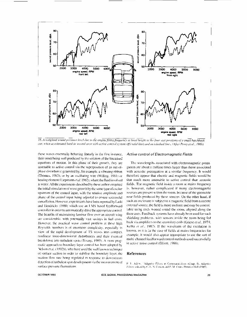
80

70

60

50 2000 3obo sdoo 5000 sdoo

engine speed. RPM from right

5 0 0 2000 3000 4OOO 5OOO 6000

engine spaed, RPM rear right

these waves essentially behaving linearly in the first instance. their onset being well predicted by the solution of the linearised equations of motion. In this phase of their growth, they are amenable to active control via the superposition of an out-of- phase disturbance generated by, for example. a vibrating ribbon (Thomas. 1983): or by an oscillating wire (Milling. 1981) or heating element (Liepmann et ~ i l . 1982). where the fluid involved is water. All the experiments described by these authors required the initial stimulation ofwave growth by the same type ofexciter upstream of the control input. with the relative amplitude and phase of the control input being adjusted to ensure successful cancellation. However, experiments have been reported by Ladd and Hendricks ( 1988) which use an LMS based feedfoiward controller in order to automatically drive the appropriate control. The benefits of maintaining laminar tlow over an aircraft wing are considerable. with potentially vast wvings in fuel costs. However, the practical wave control problem at these high Reynolds numbers is of enomious complexity. especially in view of the rapid development of TS wavcs into complex nonlinear three-dimensional disturbances and their eventual breakdown into turbulent spots (Young. 1989). A more prag- matic approach to boundary layet. control has been adopted by Nelson et al. ( 199%). who have used the well known technique of suifiice suction in order to stabilise the boundary layer. the suction flow rate being rcgulated in responsc to downstre;iiii detection of turbulent spot development \ia the measuremcnt of sui-t'acc pressure fluctuations.

Active control of Electromagnetic Fields

The wavelengths associated with electromagnetic propagation are about a million times larger than those associated with acoustic propagation at a similar frequency. It would therefore appear that electric and magnetic fields would be that much more amenable to active control than acoustic fields. The magnetic field inside a room at mains frequency is, however, rather complicated if many electromagnetic sources are present within the room, because of the geometric near fields produced by these sources. On the other hand, if such an enclosure is sub.ject to a magnetic field from a remote external source, the field is more uniform and may be controllable using coils wound round the room, aligned along the three axes. Feedback systems have already been used for such shielding problems. with sensors inside the room being fed back via amplifiers to the secondary coils (Griese et al., 1974: Kelha P I (11.. 1982). If the waveform of the excitation is known. as i t is in the case of fields at mains frequencies for example. i t would also appear appropriate to use the sort of multi-channel feedforward control methods used successfully in active noise control (Elliott, 1988).

References


G. Billout, M. A. Galland, C. H. Huu, and S. Candel, “Adaptive control of instabilities,” Proc. Recent Advances in Active Control of Sound and Vibra- tion, pp. 95-107 (1991).

B. S. Atal and M. U. Schoeder, “Apparent sound source translator,’’ U.S. Patent 3,236,949, 1962.

C. C. Boucher, S. J . Elliott and P.A. Nelson, “The effect of errors in the plant model on the performance of algorithms for adaptive feedforward control,” Special Issue of the Proceedings of Institution of Electrical Engineers 138, pp. 313-319, 1991.

J.C. Burgess, “Active adaptive sound control in a duct: a computer simula- tion,” Journal ofthe Acoustical Socieq of America 70, pp. 715-726, 1981.

C. Came, “Absorption acoustique active dans les cavites,” These presente ‘e pour obtenir le titre de Docteur de I’Universite D’Aix-Marseille I/, Faculte des Sciences de Luminy. 1987.

G. B. B. Chaplin and R. A. Smith, “The sound of silence,” Engineering (London), 218, pp. 672-673 (1978).

W. B. Conover, “Fighting noise with noise,” Noise Control 2, pp. 78-82, 1956.

P. Darlington, “Applications of adaptive filters in active noise control.” Ph.D. Thesis, University of Southampton, 1987.

P. Darlington, “Passband disturbance in active sound control systems,” Proc. Recent Advances in Active Control of Sound and Vibration, pp. 73 1-741, 1991.

A. David and S. J. Elliott, “Numerical studies of actively generated quiet zones,” to be published in Applied Acoustics, 1993.

Kg. Eghtesadi and H.G. Leventhal, “Comparison of active attenuators of noise in ducts,” Acoustics Letters 4, pp. 204-209, 1981.

S. J. Elliott and P. A. Nelson, “Algorithm for multichannel LMS adaptive filtering,” Electronics Letters 21, pp. 979-98 I , 1985.

S. J. Elliott and P. A. Nelson, “Multichannel active sound control using adaptive filtering,” Proc. ICASSP 88, pp. 2590-2593, 1988.

S. J. Elliott, “Active control of electro-magnetic fields,” U.K. Patent Appli- cation 88.18087.2, 1988.

S. J. Elliott and P. A. Nelson, “Multiple-point equalization in a room using adaptive digital filters,” J . Audio Eng. Soc. 37, pp. 899-907, 1989.

S. J. Elliott, I. M. Stothers and P. A. Nelson, “A multiple error LMS algorithm and its application to the active control of sound and vibration,” IEEE Transactions on Acoustics, Speech and Signal Processing ASSP-35, pp. 1423.1434, 1987a.

S. J . Elliott, P. Joseph, A. J. Bullmore and P. A. Nelson, “Active cancellation at a point in a pure tone diffuse sound field,” Journal ofsound and Vibration 120,, pp. 183-189, 1988a.

S. J . Elliott, 1. M. Stothers, P. A. Nelson, et al., “The active control of engine noise inside cars,” Proc. Inrer-Noise ‘88, pp. 987-990, I988b.

S. J. Elliott, P. A. Nelson, I. M. Stothers, et al., “In-flight experiments on the active control of propeller-induced cabin noise,” Journal of Sound and Vibration, 140, pp. 219-238, 1990.

S. J. Elliott, P. Joseph, P. A. Nelson et al., “Power output minimisation and power absorption in the active control of sound,” J. Acoust. Soc. Am. 90, pp. 2501 -25 12, 1991,

S. J. Elliott, C. C. Boucher and P. A. Nelson, “The behaviour of a multiple channel active control system,” IEEE Trans. Signal Processing 40, pp. 1041-1052, 1992.

S. J. Elliott, Tyndall Medal Lecture: Active control of structure-borne sound. Proc. Institute ofAcoustics 15, pp. 93-120, 1993.

L.J. Eriksson, M. C. Allie and U. A. Greiner, “The selection and application of an IIU adaptive filter for use in active sound attenuation,” Institute of Electrical and Electronics Engineers Transactions o n Acoustics. Speech and Signal Processing ASSP-35, pp. 433-437, 1987.

L. J . Erikkson and M. C. Allie, “Use of random noise for on-line transducer modelling in an adaptive active attenuation system,” Journal of the Acousti- ca/ Society ofAmerica 85, pp. 797-802, 1989.

J. E. Ffowcs-Williams, Review lecture: Anti-sound. Proc. Royal Society London A395, pp. 63-88, 1984.

S. E. Forsythe, M. D. McCollum and A. D. McCleary, “Stabilization of a digitally controlled active isolation system,” Proc. Recent Advances in Active Control of Sound and Vibration, pp. 879-889, 1991.

C. U. Fuller, C. A. Rogers and H. H. Uobertshaw, “Active Structural acoustic control with smart structures.” Proc. SPIE Conference I170 on Fibre Optic Smart Structures and Skins II, 1989.

J. R. Glover, “Adaptive noise cancellation applied to sinusoidal noise inter- ferences,” Proc. IEEE Trans., ASSP -25, pp. 484-491, 1977.

G. C. Goodwin and K. S. Sin, Adaptive Filtering Prediction and Control, Prentice Hall, 1984.

A. M. Goldman, W. E. Grossman and P. C. Fredlander, “Reduction of sound levels with antinoise in MU imaging,” Radiology 173, pp. 549-550.

A. Griese, A. A. Kalisch and H. G. Luz, “Apparatus for producing a region free from interfering magnetic fields.” U.S. Patent 3 801 877, 1974.

D. Guicking, “On the invention of active noise control,” Journal of the Acoustical Society of America 87, pp. 2251-2254, 1990.

D. Guicking, K. Karcher and M. Rollwage, “Coherent active methods for applications in room acoustics,” Journalof the Acoustical SocietyofAmerica, 78, pp. 1426.1434, 1985.

S. R. Hall and N. M. Wereley, “Linear control issues in the higher harmonic control of helicopter vibrations,” Proc. 45th Annual Forum of the American Helicopter Society, pp. 955-971, 1985.

S. Haykin, Adaptive Filter Theory, Prentice Hall, 1986.

P. Lueg, “Process of silencing soundoscillations.” U S . Patent No. 2,043,416, 1936.

M. D. Jenkins, P. A. Nelson and S. J . Elliott, “Active isolation of periodic machinery vibration from resonant sub-structures,” Proc. Winter Meeting of the American Society of Mechanical Engineers, 1990.

M. J . M. Jessel, “Sur les absorbeurs actifs,” Paper F-5-632, Proceedings 6th International Congress on Acoustics, Tokyo, 1966.

P. Joseph, “Active control of high frequency enclosed sound fields.” Ph.D. Thesis, University of Southampton, England, 1990.

MC. Junger and D. Feit, Sound, Structures and theirlnteraction, 2nd Edition, MIT Press, 1986.

V.O. Kelha et al., “Design, construction and peqformance of a large-volume magneric shield. ” I982 IEEE Trans. on Magnetics MAG-18, pp. 260-269.

K. Kido, “Reduction of noise by use of additional sound sources,” Proceed- ings of Inter-Noise ‘75, Sendai, pp. 647-650, 1975.

A. S. Knyazev and B. D. Tatttakovskii, “Abatement of radiation from flexurally vibrating plates by means of active local vibration dampers”, Soviet Phwic,r- Acoustics, 13( 1 ), pp. 1 IS- I 16, 1967.

D. M. Ladd and E. W. Hendricks. “Active control of 2-D instability waves on an axisymmetric body,” Experiments in Fluids 6, p. 69, 1988.

R.U. Leitch and M. 0. Tokhi, “Active noise control systems,” Proc IEE, 134A, pp. 525-546.

H. W. Liepmann, G. C. Brown and D. M. Nosenchuck, “Control of laminar- instability waves using a new technique.” Journal of Fluid Mechanics 118, p. 187, 1982.

N. C. MacKenzie and C. H. Hansen, “The implementation of lattice filter structure and suitable algorithm for adaptive active noise control,” Proceed- ings of Recent Advances in Active Control of Sound and Vibration, 1991.

G. D. Malyuzhinets, “An inverse problem in the theory of diffraction,” Soviet Physics, Doklady 14, pp, 118-1 19, 1969.

A. M. McDonald, S. J. Elliott and M. A. Stokes. “Active noise and vibration control within automotives.” Proc. Int. Symposium on Active Control of Sound and Vibration, Tokyo, pp, 147- 157, 1991.

R. W. Milling, “Tollmien-Schlichting wave cancellation,” Physics of Fluids 24, pp. 979. 1991.


M. Miyoshi and Y. Kaneda, “Inverse filtering of room acoustics,” IEEE Transactions on Acoustics, Speech and Signal Processing 36, pp. 145- 152, 1988.

D. R. Morgan, “An analysis of multiple correlation cancellation loops with a filter in the auxiliary path,” fEEE Transactions on acoustic.^, Speech and Signal Processing ASSP-28, pp. 454-467, 1980.

D. R. Morgan and C. Sanford, “A control theory approach to the stability and transient analysis of the Flltered-x LMS adaptive notch filter,” To appear in IEEE Trans. Sigfial Processing.

P.A. Nelson and S. J . Elliott, “Active minimisation of acoustic fields,” Journal ofTheoretiu1 and Applied Mechanics, special issue, supplement to vol. 6, pp. 39-89.

P. A. Nelson and S. J . Elliott, Active Control ofSound. Academic Press, 1990.

P.A. Nelson, A. R. D. Curtis, S. J . Elliott and A. J. Bullmore, “The minimum power output of free field point sources and the active control of sound,” Journal of Sound and Vibration 116, pp. 397-414, 1987a.

P. A. Nelson, A. R. D. Curtis, S. J . Elliott and A. J . Bullmore, “The active minimization of harmonic enclosed sound fields, Part I: Theory.” Journal of Sound and Vibration 117, pp. 1-13, 1987b.

P.A. Nelson and S. J. Elliott, “Least squares approximations to exact multiple point sound reproduction,” Proceedings of the Institute ofAcou5tic.s 10, pp. 15 1-168, 1988. (See also ISVR Memorandum No. 683, 1988).

P.A. Nelson, J . K. Hammond, P. Joseph and S. J. Elliott, “The calculation of causally constrained optima in the active control of sound,” ISVR Technical Report 147, 1988b.

P. A. Nelson, H. Hamada and S. J. Elliott, “Inverse filters for multi-channel sound reproduction,” Institute of Electronics, Information and Communica- tion Engineers of Japan, Technical Reports 91( I ) , 11-25. 199 1 .

P. A. Nelson, H. Hamada and S. J. Elliott, “Adaptive inverse filters for stereophonic sound reproduction,” To be published in fEEE Transactions on Signal Proce.c.sing, 1992a.

P. A. Nelson, J-L Rioual and M. J. Fisher, “Experiments on the active control of transitional boundary layers,” Proceedings of the Second lnternarional Congress on Recent Developments in Air- and Structure-Borne Sound and Vibration., 1992b.

H. F. Olson and E. G. May, “Electronic sound absorber,” Journal of the Acoustical Sociey of America 25, pp. 1 130- 1 136, 1953.

D.C. Perry, S. J . Elliott, I . M. Stothers and S. J. Oxley. “Adaptive noise cancellation for road vehicles,” Proceedings ofthe Institution ~fMechanical Engineers Conference on Automotive Electronics, pp. 150- 163, 1989.

A. Roure, “Self adaptive broadband active sound control system,” Jouniul of Soundand Vibration 101, pp. 429-441, 1989.

M. R. Schroder, “Computer models for concert hall acoustic?.” American Journal of Physics 14, pp. 467-47 I , 1973.

L. A. Sievers and A. H. von Flotow, “Comparison and extension of control methods for narrowband disturbance rejection,” To be published in / € € E Trans. Signal Processing, 1992.

S. D. Snyder and C. H. Hansen, “Design considerations for active noise control systems implementing the multiple input, multiple output LM5 algorithm,” Joirrnul ($Sound and Vibrution, 159, pp. 157- 174, 1992.

M.M. Sondhi and D. A. Berkley, “Silencing echoes on the telephone net- work,” Proc. fEEE 68, pp. 948-963, 1980.

J . C. Stevens and K. K. Ahuja, “Recent advances in active noise control,” AIAA Joumal29, pp. 1058-1067, 1991.

1. M . Stothers, T. J . Saunders, A. M. McDonald and S. J . Elliott, “Adaptive feedback control of sunroof flow oscillations,” Proc. fnstitute of Acoustics 15, pp. 383-394, 1993.

D.C. Swanson, “Active attenuation of acoustic noise: past, present and future,” ASHRE Transactions 96, pp. 63-76, 1990.

D.C. Swanson, “Lattice filter embedding techniques for active noise control,” Proceedings Inter-Noise 91, 1, pp. 165-168.

M. A. Swinbanks, “The active control of sound propagating in long ducts,” Journal of Sound and Vibrution 27, pp. 41 1-436, 1973.

N. Sundararajan, J . P. Williams and R. C. Montgomery, “Adaptive modal control of structural dynamic systems using recursive lattice filters,” AIAA J. Guidance, Control and Dynamics 8, pp. 223-229, 1985.

T. J . Sutton. S. J. Elliott, P. A. Nelson and 1. Moore, “Active control of multiple-source random sound in enclosures,” Proceedings Institute of Acoustics, 12, pp. 689-693, 1989.

T. J. Sutton and S. J. Elliott, “Frequency and time domain controllers for the attenuation of harmonic vibrations in nonlinear structural systems,” Proc. Institute of Acoustics 15, pp. 775-784, 1983.

A. S. W. Thomas, “The control of boundary layer transition using a wave superposition principle,” Journal ofFluid Mechunics 137, p. 233, 1983.

D. R. Thomas, P. A. Nelson and S. J. Elliott, “The active control of the transmission of sound,” Proc. Institute ofAcoustics 12, pp. 605-612, 1990.

M. C. J. Trinder and P. A. Nelson, “Active noise control in finite length ducts,” Journal of Sound and Vibration 89, pp. 95-105, 1983.

S. Uto. H. Hamada, T. Miura et al., “Audio equalizers using multi-channel adaptive filters,’‘ Proceedings of the International Symposium on Active Control ($Sound and Vibrarion (Tokyo), pp. 421-426, 1991.

I. Veight, “A lightweight headset with an active noise compensation,” Proc. Inter-Noise ‘88, pp. 1087-1090, 1988.

G. E. Wamaka “Active attenuation of noise: The state of the art,” Noise Control Engineering 18(3), pp. 100-1 10, 1982.

P. E. Wellstead and M. B. Zarrup, SelfTiming Systems, John Wiley, 1991.

P. D. Wheeler, “Voice communications in the cockpit noise environment- the role of active noise reduction.” Ph.D. Thesis, University of Southampton, England. 1986.

P. D. Wheeler, “The role of noise cancellation techniques in alrcrew voice communications systems,” Proc. Royal Aeronuutical Society Symposium on Helmets and Helmet-Mounted Devices, 1987.

B. Widrow, J. R. Glover, J. M. McCool et al., “Adaptive noise cancelling principles and applications,” Proceedings IEEE 63, pp. 1692-1716, 1975.

B. Widrow and S. D. Steams, Aduptile Signal Processing. Prentice Hall, Englewood Cliffs, New Jersey (1985).

B. Widrow, D. Shur and S. Shaffer, “On adaptive inverse control,” Proceed- ing.y qf‘the 15th ASILOMAK Conference on Circuits, Systems and Computers, 185.195, 1981.

A. D. Young, Roundaq Layerv. Blackwell Scientific, Oxford, 1989.


Documents

Active noise control - Institute of Sound and Vibration Research

References

OCTOBER 1993 IEEE SIGNAL PROCESSING MAGAZINE 33