Embed Size (px)
Citation preview
AD-A009 138
DESIGN AND CALIBRATION OF THE ARL MACH 3 HIGH REYNOLDS NUMBER FACILITY
A. W. Fiore, et al
Aerospace Research Laboratories Wright-Patterson Air Force Base, Ohio
January 1975
DISTRIBUTED BY:
KliJi National Technical Information Service U. S. DEPARTMENT OF COMMERCE

... . .
... -
UNCLASSIFIED SeCURITY CLASSIFICATION OF THIS PAGE (Whtn Data EnlBiodJ
REPORT DOCUMENTATION PAGE READ INSTRUCTIONS BEFORE COMPLETING FORM
I REPORT NUMBER
ARL 75-0012 2 GOVT ACCESSION NO 3 RECIPIENT'S CATALOG NUMBER
Al)-/) Co 7 iM 4. TITLE (and Submit)
DESIGN AND CALIBRATION OF THE ARL MACH 3 HIGH REYNOLDS NUMBER FACILITY
5. TYPEOF REPpRT A PERIOD COVERED Final Technical July 1965 - December 1972 6. PERFORMING ORG. REPORT NUMBER
7. AUTHORfi; ». CONTRACT OR GRANT NUMBERfsJ
A. W. Fiore; D. G. Moore; D. H. Murray and J. E. West, Maj. USAF
9 PERFORMING ORGANIZATION NAME AND ADDRESS
Fluid Mechanics Research Laboratory and Theoretical Aerodynamics Rsch Lab (ARL/LF & LH) Wright-Patterson AFB, OH 45433
10. PROGRAM ELEMENT, PROJECT, TASK 4RFl.a WDRKJIWIT NUMBERS
61102F; 7065-14-28 61102F; 7064-02-06
11, CONTROLLING OFFICE NAME AND ADURESS
Aerospace Research Laboratories (AFSC) Bldg. 450, Area B Wright-Patterson AFB, OH 45433
12. REPORT DATE
January 1975 13. NUMBER OF PAGES
M 14 MONITORING AGENCY NAME & ADDRESSr*/ dilferenl Irom ComroJKnO Ollice) 15. SECURITY CLASS, frl (Jii,i reporl)
Unclassified 15a. DECL ASSIFICATION DOWNGRADING
SCHEDULE
16. DISTRIBUTION STATEMENT fol IhU Reporlj
Approved for public release; distribution unlimited.
17. DISTRIBUTION STATEMENT (al (he abstract tntvred In Block 20, II dillerenl Irom Report)
IB. SUPPLEMENTARY ^TES
19. KEY WORDS fConftnua on reverse aide it necessary and Menf//y by block number)
Wind Tunnel Mach Number 3 High Reynolds Number
Design Calibration
PRICES SUBJECT TO CHANGE 20. ABSTRACT (Continue on ravers« aide It necessary mnd Identify by block number)
The design philosophy and details of the ARL Mach 3 High Reynolds Number Facility are described and the results of extensive calibration tests are presented. The facility is an intermittent cold flow wind tunnel having a constant area test section 8 inches wide and 8.2 inches high, with a test rhombus 23 inches long. It operates in a blowdown mode using dry compressed air which is exhausted to the atmosphere through a silencer. Tunnel stagnation pressures range from 40 psia to 570 psia, with stagnation temperatures in a range from 400 degrees Rankine to 500 degrees Rankine depending upon ambient conditions. The corresponding free
DD FORM 1 JAN 71 ]473 ED,'r,rtfcl ^P ' WAV/ ««i \K nR<;ni FTF
Reproduced by
NATIONAL TECHNICAL INFORMATION SERVICE
US Department of Commerce Springfield, VA. 22151
UNCLASSIFIED PURITY CLASSIFICATION (JF THIS PAGE (When Dele Enlerrd)

pg.Pfj m^j'nmmmKf^mmK 'vm X ' ' "•' ' ' "" -.—J.wi-T^rpw, wnyAWR"«^1' " ■
■ ■ n
UNCLASSIFIED SECURITY CLASSIFICATION OF THIS PAGEfWun Dmlm Enlermd)
20. (Cont'd)
stream unit Reynolds numbers vary from 7 million per foot to 140 million per foot The tunnel has been operated with a vacuum exhaust which permitted stagnation pressures as low as 4.2 psia with a corresponding free stream unit Reynolds number of 0.8 million per foot. The aerodynamic calibration measurements were made at nominal stagnation pressures of 100, 300 and 500 psia with an average stagnation temperature of 480 degrees Rankine. Test rhombus determinations included lateral and longitudinal Mach number distributions and flow angularity measurements. A limited number of tunnel blockage tests were performed and some ,'iow visualization tests were made to determine characteristics of the start-stop process.
SECURITY CLASSIFICATION OF THIS PAGECIfhon DatM Entered)

-■■-: '- ■ -"'"■""
■'■■ MMclM . .
PREFACE
This report was prepared jointly by the Fluid Mechanics Research
Laboratory of ARL under Project 7065, "Aerospace Simulation Techniques,"
and by the Hypersonic Research Laboratory of ARL under Project 7064, "High
Velocity Fluid Mechanics." This report covers the design and calibration of
the ARL Mach 3 High Reynolds Number Facility.
The authors wish to acknowledge the significant contributions of
Mr. Emil Walk, formerly of the Fluid Mechanics Research Laboratory, as the
project monitor, and Ms. Constance M. Woehle and Mrs. Shirley E. McGrath
for typing the manuscript.

■
•TABLE OF CONTENTS
SECTION PAGE
I INTRODUCTION 1
II DETAILED WIND TUNNEL DESIGN . 4
1. HIGH PRESSURE AIR SYSTEM 5
a. Storage Tanks 6
b. Manifolding 6
c. Piping 6
2. WIND TUNNEL PROPER 7
a. Tunnel Foundation 7
b. Pressure Control System 8
c. Settling Chamber 9
d. Entrance Bellmouth 12
e. Nozzle 12
f. Test Section 17
g. Model Support Systems 19
h. Diffuser 20
3. EXHAUST SYSTEM 22
a. Vacuum 23
b. Atmospheric 24
III WIND TUNNEL CONTROLS AND INSTRUMENTATION 25
1. SYSTEM STATUS MONITORS 26
2. INTERLOCK SYSTEM 28
3. STAGNATION PRESSURE CONTROL SYSTEM 30
a. Process 30
b. Pressure Sensor 31
■m

■
.-*.- ,-,-.,.v - - -— m —•-——^—-—'-
TABLE OF CONTENTS (CONT'D)
SECTION PAGE
c. Programmer 31
d. Controller 31
e. Servo Amplifiers 32
f. Process Control Loop 32
4. VALVE RESPONSE TESTS 33
5. WATER HAMMER 33
6. CONTROLLER RESPONSE 35
7. MODEL SUPPORT SYSTEM CONTROL 35
IV AERODYNAMIC CALIBRATION OF THE WIND TUNNEL 37
1. THE LATERAL MACH NUMBER DISTRIBUTIONS 37
2. THE LONGITUDINAL MACH NUMBER DISTRIBUTIONS 43
3. THE TUNNEL EMPTY MACH NUMBER DISTRIBUTION 45
4. THE CENTERLINE RMS MACH NUMBER 46
5. FLOW ANGULARITY MEASUREMENTS 46
6. BLOCKAGE TESTS 52
7. REMARKS ON FLOW LIMITATIONS 53
V CONCLUSIONS 56
REFERENCES 60
APPENDIX: BASIC DESIGN CONSIDERATIONS 131
1. INPUT DESIGN PARAMETERS 131
a. Test Section Mach Number 131
b. Desired Model Sizes 132
c. Desired Reynolds Number Range 132
d. Desired Run Times 132
iv

■■
TABLE OF CONTENTS (CONT'D)
SECTION PAGE
2. CALCULATED PARAMETERS 133
a. Tunnel Stagnation Conditions 133
b. Tunnel Pressure Ratio, A 135
c. Test Section Size 136
d. Mass Flow 137
e. Exhaust System 138
f. Air Supply 141
3. OUTPUT DESIGN PARAMETERS 142
a. Test Section Mach Number 143
b. Test Section Size 143
c. Stagnation Temperature 144
d. Stagnation Pressure 145
e. Run Time 145
f. Exhaust System 146
g. Performance Envelope 146
LIST OF SYMBOLS 169

■
,,„,,..,,..|.l., .11 ! .■--.^^~r-
LIST OF ILLUSTRATIONS
FIGURE PAGE
1 Perspective Drawing of the ARL Mach 3 High Reynolds Number Facility 62
2 Estimated Pressure Drop in Distribution Piping as a Function of Mass Flow and Storage Pressure 63
3 Mach 3 Nozzle Configuration 64
4 Original Exhaust System Configuration-Vacuum 65
5 Rise of Sphere Pressure With Run Time for a Range of Stagnation Pressures 66
6 Present Exhaust System Configuration-Atmospheric 67
7 Mach 3 Process Diagram 68
8 Logic Symbol Convention 69
9 Control Valve Status 69
10 Isolation Valve Control Logic 70
11 Run Interlock Logic 71
12 Exhaust Valve Control Logic 71
13 Alarm System Logic 72
14 Stagnation Pressure Control System 73
15 Mach 3 Process Control Loop 74
16 Valve Response Test-2 inch Valve 75
17 Valve Response Test-6 inch Valve 76
18 Controller Test-2 inch Valve 77
19 Controller Test-6 inch Valve 78
20 Scale Drawing of the Mach 3 Nozzle and Test Section 79
21 Scale Drawing of the Mach Number Survey Rake 80
22 Survey Rake Reference Axis and Nomenclature 81
vi

r,m.,.^,.,,—.T- , J ,M,m,,lm^mm^mtmm^W,„„,„km,r,„.r,l.... -1-,^^™!„,
■ ■ ■
LIST OF ILLUSTRATIONS (CONT'D)
FIGURE PAGE
23a Impact Mach Number Versus y/As for xp/xr = - 0.690 at p0 = 109 psia and T0 = 430oR 82
23b Impact Mach Number Versus V/AS for xp/xr = - 0.345 at p0 = 111 psia and T0 = 477°R 83
23c Impact Mach Number Versus y/As for xp/xr = 0 at p0 = 111 psia and T0 = 4840R 84
23d Impact Mach Number Versus y/As for xp/xr = + 0.345 at p0 = 108 psia and T0 = 4770R 85
23e Impact Mach Number Versus y/As for xp/xr = + 0.690 at p0 = 103 psia and T0 = 4720R 86
24a Impact Mach Number Versus y/As for xp/xr = - 0.690 at p0 = 306 psia and T0 = 4680R 87
24b Impact Mach Number Versus y/As for xp/xr = - 0.345 at p0 = 316 psia and T0 = 4820R 88
24c Impact Mach Number Versus y/As for xp/xr = 0 at p0 = 323 psia and T0 = 491
0R 89
24d Impact Mach Number Versus y/As for xp/xr = + 0.345 at p0 = 313 psia and T0 = 483^ 90
24e Impact Mach Number Versus y/As for xr = + 0.690 at p0 = 318 psia and TQ = 476°R 91
25a Impact Mach Number Versus y/As for xp/xr = - 0.690 at Po = 518 psia and T0 = 4780R 92
25b Impact Mach Number Versus y/As for xp/xr = - 0.345 at p0 = 520 psia and T0 = 4910R 93
25c Impact Mach Number Versus y/As for xp/xr = 0 at p = 532 psia . and T0 = 499
0R 94
25d Impact Mach Number Versus y/As for xp/xr = +0.345 at p0 = 517 psia and T0 = 491;bR 95
0.690 at 25e Impact Mach Number Versus y/As for xp/xr = + p0 = 523 psia and T0 = 486lbR 96
26a Centerline Mach Number Versus Longitudinal Distance for Po = 100 psia, T0 = 4680R, where Re/ = 20.69 x 10⁶ per foot . . 97
vn

.
FIGURE
26b
26c
27a
27b
27c
28a
28b
28c
29a
29b
29c
30
31
32
33
34a
34b
LIST OF ILLUSTRATIONS (CONT'D)
Centerline Mach Number versus Longitudinal Distance for Po = 300 psia, T0 = 480.06oR, where Re/H = 59.2 x 10⁶ per foot .
Centerline Mach Number versus Longitudinal Distance for Po = 500 psia, To = 489.05oR, where Re/£ = 95.0 x 10⁶ per foot .
Mach Number versus Longitudinal Distance for r/As = ± 1.0 at p0 = 100 psia, T0 = 468.40R and Re/£ = 20.69 x 10⁶ per foot
Mach Number versus Longitudinal Distance for r/As = ± 1.0 at Po = 300 psia. To = 480.06oR and Re/l = 59.2 x 10⁶ per foot
Mach Number versus Longitudinal Distance for r/As = ± 1.0 at Po = 500 psia, T0 = 489.05oR and Re/Z = 95,0 x 10⁶ per foot
Mach Number versus Longitudinal Distance for r/As = ± 2.0 at Po ~ 100 psia, To = 468.40R and Re/Z = 20.69 x ID6 per foot
Mach Number versus Longitudinal Distance for r/As = ± 2.0 at Po = 300 psia. To = 480.06^ and Re/Z = 59.2 x 10⁶ per foot
Mach Number versus Longitudinal Distance for r/As = ± 2.0 at Po = 500 psia, T0 = 489.05oR and Re/£ = 95.0 x 10⁶ per foot
Mach Number versus Longitudinal Distance for r/As = ± 3.0 at Po = 100 psia. To = 468.40R and Re/£ = 20.69 x 10⁶ per foot
Mach Number versus Longitudinal Distance for r/As = ± 3.0 at Po = 300 psia. To = 480.06oR and Re/£ = 59.2 x 10⁶ per foot
Mach Number versus Longitudinal Distance for r/As = ± 3.0 at Po = 500 psia. To = 489.05oR and Re/£ = 95.0 x 10⁶ per foot
Wall Mach Number versus Longitudinal Distance for Tunnel Empty Condition with Reynolds Number as a Parameter ....
Root-Mean=Square Mach Number versus Unit Reynolds Number Per Foot
Scale Drawing of Flow Angularity Wedge
Scale Drawing of Flow Angularity Cone
Normalized Surface Pressure Difference versus Angle of Attack at xp/xr = - 0.690 for po = 103.6 psia with Settling Chamber Spreader Cone Tip Downstream ....
Normalized Surface Presswre Difference versus Angle of Attack at xp/xr = - 0.34b for po = 100.6 psia with Settling Chamber Spreader Cone Tip Downstream ....
PAGE
98
99
100
101
102
103
104
105
106
107
108
109
110
in
112
113
114
vm

-.„,.,-,-,, ■
LIST OF ILLUSTRATIONS (CONT'D)
FIGURE PAGE
34c Normalized Surface Pressure Difference versus Angle of Attack at xp/xr = 0 for po = 100.6 psia with Settling Chamber Spreader Cone Tip Downstream 115
34d Normalized Surface Pressure Difference versus Angle of Attack at xp/xr » 0.345 for p0 = 95.0 psia with Settling Chamber Spreader Cone Tip Downstream 116
34e Normalized Surface Pressure Difference versus Angle of Attack at xp/xr = 0.690 for p0 = 95.4 psia with Stagnation Section Spreader Cone Tip Downstream 117
35 Velocity Profile in a Model Settling Chamber with and without a Spreader Cone . 118
36 Flow Angularity versus Lateral Distance at xp/xr = 0 (Rhombus Center) with the Spreader Cone Tip Upstream .... 119
37 Flow Angularity versus Lateral Distance at xp/xr = 0 (Rhombus Center) with the Spreader Cone Tip Downstream ... 120
38 Unit Reynolds Number Effect on the Flow Angularity at xp/xr - 0 (Rhombus Center) 121
39 Flow Angularity versus Lateral Distance with Longitudinal Distance as a Parameter for pg = 100 psia, T0 = 470oR, M = 2.99 and Re/£ = 20.6 x 10g per Foot 122
40 Flow Angularity versus Longitudinal Distance at z/(b/2) = + 0.5 (East Side) with the Spreader Cone Tip Downstream . . 123
41 Flow Angularity versus Longitudinal Distance at 2/(b/2) = 0 (Centerline) with the Spreader Cone Tip Downstream 124
42 Flow Angularity versus Longitudinal Distance at z/(b/2) = - 0.5 (West Side) with the Spreader Cone Tip Downstream . . 125
43 Flow Angularity versus Probe Roll Angle at the Center of the Test Rhombus (xp/xr = 0) 126
44 Tunnel Blockage versus Mach Number 127
45 Schlieren and Shadowgraphs of Flow Over a Two-Dimensional Wedge at M = 3.0 and Re/£ = 20.66 x 10⁶ per Foot for a = 0° and a = 4° 128
46 Schlieren and Shadowgraphs of Flow Over a Two-Dimensional Wedge at M = 3.0 and Re/£ = 20.66 x 10⁶ per Foot for a = 7° and a = 10° 129
IX

■
LIST OF ILLUSTRATIONS (CONT'D)
APPENDIX
FIGURE PAGE
A-l Design Flow Chart 150-153
A-2 Streamwise Location of Transition on a Model at Mach 3 as a Function of Free Stream Unit Reynolds Number 154
A-3 Effect of Air Condensation on Tunnel Operating Range at a Mach Number of 3 155
A-4 Rate of Change of Free Stream Unit Reynolds Number with Tunnel Stagnation Temperature at Mach 3 156
A-5 Variation of Free Stream Unit Reynolds Number with Tunnel Stagnation Pressure and Temperature 157
A-6 Tunnel Pressure Ratio Requirements I58
A-7 Variation of Maximum Model Size with Fineness Ratio for Shock Reflection Limited Cases 159
A-8 Variation of Maximum Base Diameter for Starting Tunnel with Blunt Cone Models 160
A-9 Variation of Maximum Cone Length with Inviscid Test Section Size for Shock Reflection Limited Cases 161
A-10 Variation of Maximum Wedge Length with Inviscid Test Section Size for Blockage Limited Cases 162
A-ll Mass Flow Per Unit Test Section Area as a Function of Tunnel Stagnation Conditions 163
A-12 Variation of Silencer Size with Test Section Size for a Silencer Intake Velocity of 100 ft/sec 164
A-13 Variation of Required Vacuum Volume with Test Section Size for a 60 Second Run at a Unit Reynolds Number of 1.2 x 10⁶ per foot. . 165
A-14 Variation of Air Storage Volume Requirements with Test Section Size and Operating Pressure 166
A-15 Maximum Model Reynolds Number Attainable as a Function of Inviscid Test Area 167
A-16 Predicted Tunnel Performance Envelope 168

LIST OF TABLES
TABLE PAGE
I Mach 3 Nozzle Coordinates 15
A.I Turbulent Flow Testing Capabilities 148
A,II Laminar Flow Testing Capabilities with an Atmospheric Exhaust . 149
xi

SECTION I
INTRODUCTION
In July 1965 the Aerospace Research Laboratories at Wright-Patterson Air
Force Base began to give serious consideration to the construction of a high
Reynolds number aerodynamic test facility, the intention being to study
turbulent flow phenomena at supersonic and low hypersonic speeds. The need
for aerodynamic test data at high Reynolds numbers, particularly in this
speed range, had become increasingly apparent in the course of identifying
critical problem areas associated with the fluid mechanics of new and advanced
Air Force systems. Increased attention was being given to "low and fast"
aircraft and other weapon delivery systems, and there was also a trend toward
larger rocket boosters and reusable launch vehicles. Fundamental information,
such as heat transfer data, was scant in the appropriate Mach number/Reynolds
number range, and extrapolation was virtually impossible. It was clear that
there was a need for experimental data pertaining to pure turbulent boundary
layers, flow interactions, heat transfer rates, skin friction values, wake
characteristics, and aerodynamic stability under turbulent flow conditions.
The Mach number range of particular interest appeared to extend from Mach 2 Q
to Mach 6, WK.,i Reynolds numbers ranging up tO'10 or greater. A thorough
review of existing supersonic and hypersonic facilities throughout the
country^ " ' revealed that very few were designed for operation at free
stream unit Reynolds numbers much above 10 per foot. The principal exceptions
were the shock tunnels which are unsuitable for some types of detailed flow
studies due to their extremely short running times. In view of the very
limited high Reynolds number testing capability which the country had, there
appeared to be little doubt that the establishment of a high Reynolds number

"■ ■
Simulation capability at ARL would be a sound and timely investment in a
research and development tool necessary for servicing current and future needs
of Air Force systems.
Convinced of the need, ARL undertook to study the problem of providing
the desired simulation capability as quickly and as inexpensively as possible,
using existing technology wherever possible. It was apparent early in the
study that the Mach number range could not be satisfactorily covered with one
flow channel. The logical approach appeared to be to have a facility con-
sisting of an unheated leg for low Mach numbers and a heated leg for higher
Mach numbers, with as much common equipment as possible. It was decided that
representative Mach numbers for the two legs should be Mach 3 and Mach 6,
with no immediate provisions to be made tor varying the test section Mach
number of each leg.
Based upon the above decisions, a preliminary design study was made in
which the requirements for major components were analyzed to establish the
overall technical feasibility of the approach, and to ascertain costs, man-
power requirements, and the effect of the facility on the existing research
complex. Test section sizes and run times were of prime consideration due
to their direct impact on facility size and facility service demands. Follow-
ing this study, which concerned itself with conventional blowdown wind tunnel
designs, two intensive reviews and several small studies were made to see if
new or emerging techrology could be expected to produce significantly superior
facilities which would warrant a delay in the construction of a new facility.
Since this did not appear to be the case, in February 1967 the decision was
made to proceed with the design and construction of the Mach 3 leg of the
facility. In-house work on the detailed design started immediately and

construction effected by the FluiDyne Engineering Corporation of Minneapolis,
Minnesota, was completed approximately two years later. This was followed by
an exhaustive series of component check-out tests comprising well over one
hundred tunnel runs. These were completed during March 1969. The installation
and check-out of research instrumentation occupied the facility until
September 1969, when calibration tests were started. These were completed in
July 1970 and regular aerodynamic testing began during August 1970. The
first aerodynamic test report containing data obtained from the tunnel was
published in October 1971.'7'
The purpose of this report is to provide a single published source of
information on the facility. It is intended to be useful to those preparing
for tests in the facility and to those interpreting data obtained in the
facility. For the interest of those engaged in the design and construction
of similar facilities, an appendix covering the basic design considerations
which led to the detailed design described in Section II of the report has
been included.

SECTION II
DETAILED WIND TUNNEL DESIGN
The detailed design of the wind tunnel was based upon the design
criteria and calculations discussed in the appendix. A facility design goal
was established, namely, the safe production and control of a uniform Mach 3 o
flow, having a free stream unit Reynolds number (IteJ of 10 per foot at a oo
stagnation pressure (P ) of 570 psia and a stagnation temperature (T ) of
500oR. The test section size was to be nominally 8 inches square, with
allowances for nozzle boundary layer growth. The tunnel was to be designed
for direct exhaust to the atmosphere, and for exhaust to an existing 3
100,000 ft vacuum sphere capable of being evacuated to a pressure of 1 torr.
Based upon this design goal, a facility concept was developed, and expanded
to the point of specifying design or performance criteria for all significant
systems, subsystems and components. The end result of this effort is depicted
in the facility perspective presented in Figure 1.
In order to identify the major components in the system, a brief
description of the facility is given in terms of the path taken by the air
through the facility. Air passes from a high pressure storage area through
two parallel four-inch diameter Schedule XXS high pressura pipes into two
remotely controlled isolation valves, which are manifolded together on the
downstream side. This manifold connects to the common intake of a six-inch
diameter pressure control valve and a two-inch diameter pressure control
valve, of which both are hydraulically actuated. The two valves are connected
in parallel to permit individual selection for operation at either high or
low mass flow. Air passes from the active control valve to the settling
chamber through a wide angle expansion, which incorporates a flow spreader to

promote a uniform velocity profile. The settling chamber experiences the
full stagnation pressure of the flow, and is fitted with a rupture disc to
protect it from overpressurization in the event of control valve failure.
Screens in the settling chamber help to reduce the scale and intensity of the
turbulence in the flow prior to acceleration through the aerodynamic nozzle to
the test section Mach number of 3. After the air passes over the model in the
test section, it undergoes some deceleration in the diffuser, and then enters
the downstream ducting and exhaust system. Further details on the facility
components are given below with the same flow sequence.
1. HIGH PRESSURE AIR SYSTEM 3
The ARL high pressure air system includes over 15,000 ft of 3000 psi
air storage for the use of many special purpose test rigs and wind tunnels.
Three four-stage reciprocating air compressors are able to take atmospheric
air and deliver it to the storage vessels at a combined mass flow rate of
1.0 lbm/sec. In addition to removal of condensed water and oil by separators,
oil vapor is removed by a special "oil-sorb" unit. The saturated air is
then dried by passage through one of two automatically cycled silica gel
drying towers, which permit dew points as low as -100oF to be achieved. Fine
mesh filters assure that the air passing to the storage tanks is essentially
particulate free. One 8250 ft section of the storage area is normally
available to the facility. The maximum system pressure is 3000 psia, but the
pressure available to the Mach 3 facility is often lower due to the operation
of other facilities. The air consumption/recovery ratio can be as high as
200 to 1 for this facility, which means that a sequence of three 60 second
high pressure runs consumes more air than can be recovered in ten hours of
compressor plant operation. Further details of the high pressure air system
of interest to this particular facility are given below.
5

■■
a. Storage Tanks 3
The 8250 ft of storage volume referred to above Is made up of
3 3 twenty-eight 250 ft tanks and one 1250 ft tank. The tanks contain no heat
sink materials and are completely exposed to atmospheric conditions. The
small tanks each have a 2 in.-2500# ASA Ring Joint Flange outlet connection.
The corresponding internal diameters are 1.503 inches and 2.300 inches,
respectively, which are sufficient to keep local outlet velocities below
50 ft/sec for the small tanks and 100 ft/sec for the large tank.
b. Manifolding
The storage tanks are connected to two four-inch diameter Schedule
XXS pipe manifolds through individual high pressure gate valves. Each pipe 3
manifold is connected to fourteen 250 ft tanks, but only one is connected 3
to the 1250 ft tank. The manifolds therefore have connected volumes of 3 3
3500 ft and 4750 ft . Under normal conditions corresponding manifold air
velocities should not exceed 150 ft/sec and 200 ft/sec, respectively.
c. Piping
The manifolds are connected to the facility by independent
four-inch diameter Schedule XXS pipes, each incorporating a pressure balance
four-inch high pressure shut-off gate valve upstream of the corresponding
facility isolation valve. With the usual allowances for elbows, valves, tees
and reducers, the approximate equivalent lengths of the two supply lines,
including manifolds, are 400 ft and 300 ft, the longer length being associated 3
with the manifold connected to the 1250 ft tank. Figure 2 shows how the
pressure drop increases with the mass flow rate for the combined supply lines
for a range of storage pressures. Losses have been estimated up to, but

T
excluding, the control valves. These curves can be used to establish the
minimum storage pressure (PST) required for a run, providing allowances are
made for the pressure drop through the control valve, and for the pressure
drop in the storage vessels due to the air consumed and the associated exp
sion cooling. From an examination of the wide range of operating conditions
possible, a good rule-of-thumb would be to have a minimum storage pressure of
at least th^ee times the tunnel stagnation pressure.
All of the components of the high pressure air system described
above wore subjected to a hydrostatic test at 4500 psig prior to use.
2. WIND TUNNEL PROPER
The wind tunnel proper comprises those mechanical elements essential to
the conveyance, control, and aeodynamic conditioning of the test air. The
design of the most important elements is discussed below, primarily from the
standpoint of function and physical characteristics. Control and instrumenta-
tion aspects of the wind tunnel are discussed in Section III.
a. Tunnel Foundation
The tunnel foundation has the function of supporting the tunnel
components, the upstream piping, and a portion of the downstream ducting. It
is designed to resist the horizontal thrust loads that occur at maximum mass
flow conditions, and the vertical loads that would occur following the rupture
of either of two eight-inch rupture discs. By combining the foundations of
the various components into one unit, the opposing horizontal forces are
cancelled out in the foundation, and are not transmitted to the ground. The
foundation is of reinforced concrete containing sleeved anchor bolts for
component mountings. It is vibrationally isolated from the building slab by
a 1/2-inch peripheral expansion joint.

b. Pressure Control System
The high pressure air control system comprises two isolation valves,
one primary control valve, one secondary control valve, one equalization
valve, and a control system. The function of the overall system is to
control discretely the stagnation pressure in the settling chamber during a
run.
(1) Isolation Valves
The two isolation valves are four-inch Grove Series G gate
valves which are provided to assure positive remote isolation of the facility
from the high pressure air supply system. In addition, the electro-hydraulic
actuators operate fast enough (less than one second) for the valves to be used
as shut-off valves under emergency conditions if the pressure control valve
malfunctions in the open position. An adjustable differential pressure
switch across the isolation valves can be used to time-sequence the operation
of the control valves. In the event of power failure, the valves are
hydraulically actuated to the closed position to provide a failsafe condition.
(2) Pressure Control Valves
The primary pressure control valve is a six-inch Annin
Model 4510 valve, with a C.G.S. Model 361 electro-hydraulic actuator. It has
a Cv of 290 and is used to control mass flows over a range of 50 to 200
lb /sec. The secondary pressure control valve is a two-inch Annin Model 4510,
with a C.G.S. Mode? 321 actuator. It has a Cv of 35 and ir used to control
mass flows below 50 lb /sec. Both valves have linear characteristics, and
can be operated in either an automatic mode or manual mode to achieve a set-
point operating pressure in the settling chamber.

(3) Eoualization "alve
The equalization valve is a Jamesbury 3/4-inch Type HP ball
valve which provides a means of pressurizing the upstream side of the control
valves prior to operation of the isolation valves. The equalization valv? is
fitted with a failsafe spring-loaded air cylinder operator which closes upon
air or electrical power failure.
(4) Control Elements
The stagnation pressure control elements consist of a
programmer, two controllers, two servo amplifiers, and three pressure sensing
transducers which are integrated with the control valves and actuators to form
the control loops for establishing and maintaining the desired air flow
conditions. These form a process control system which is described later in
Section III.
c. Settling Chamber
The settling chamber has the function of conditioning the air before
it passes through the nozzle. Conditioning includes promoting a uniform
velocity profile at the nozzle entrance, and reducing the scale and intensity
of turbulence. In addition, the settling chamber volume must be sufficient
to eliminatp time variations in the sensed stagnation pressure, so that any
control valve perturbations are not amplified in the control loop. Particular
features of the settling chamber assembly are discussed below.
(1) Shell Assembly
The settling chamber shell assembly constitutes a pressure
vessel, designed for 700 psi dir service in accordance with Section VIII of
the ASME code for unfired pressure vessels. ^ The upstream end of the
welded structure incorporates a flanged manifold for mounting the two control
^ ■,..■•-*
valves, followed by a 90° long radius elbow. A conical wide-angle expansion
member connects the downstream side of the elbcw to the main cylindrical
member of the shell. This main member incorporates a downstream connection
flange, thrust mount pads, and a rupture disc assembly mounting flange. The
eight-inch diameter rupture disc is sandwiched between flanges, and is suffi-
cient to prevent overpressurization of the vessel in the event of control
valve failure (wide open) at the maximum system pressure of 3000 psi. Thrust
forces are transmitted by the brackets to the tunnel foundation through a
steel thrust support member. Welded to the top of vessel are three mounting
pads for the tunnel siJe-wall swing-arm assembly. The settling chamber
diameter was chosen to provide a mass-averaged velocity of approximately
30 ft/sec. One of the primary concerns in the design was that äir temperatures
would on occasion be considerably below -20oF, where many carbon and low
alloy steels begin to suffer serious decreases in impact resistance. Instead
of using a stainless steel, or of complying with the special material impact
tests requirements, the code option of designing to a pressure equal to
2 1/2 times the maximum working pressure was chosen. The cylindrical section
of the vessel did not require special low temperature consideration due to the
use of an inner steel liner not subject to pressure loads. Since run tim2s
are short, on an absolute time scale, the pressure vessel itself does not
reach the low air flow temperature.
(2) Flow Spreader
The limited building space available to the facility made it
necessary to have a 90° long radius elbow, immediately followed by a wide-
angle diffuser section, in order to make the transition from the high pressure
piping to the full settling chamber diameter. Because of the high rrass flow
10

i^.|l...IV»Tilv.v,n,w.^.w.!l -• --
rates there was considerable concern that turbtlence and asymmetry at the
control valve, and centrifuging in the elbow, would lead to significant flow
nonuniformities in the settling chamber. To counter this possibility it was
decided to incorporate a perforated cone with the wide-angle diffuser. The
idea of using such a device was not new, having been mentioned by Ferri and (g)
Bogdonoff as early as 1954/ ' but no experimental performance data were
available. In fact, there was considerable room for debate on whether such a
device might be more effective pointing downstream, rather than upstream as
depicted in the few literature references discovered/ " ' In view of this,
some small scale studies were made by ARL to determine the influence of
orientation on effectiveness. These studies are discussed further in connec-
tion with flow angularity measurements in Section IV. Pending the outcome of
the small scale tests, the flow spreader was designed to be reversible. The
cone has a semi-vertex angle of 45° (the semi-expansion angle of the wide-angle
diffuser is 30°) and is fabricated from 3/4-inch thick perforated steel plate
having .707 in. diameter holes and a porosity of 36%. The base is reinforced
with a steel ring to support and align the cone inside the shell. Movement
of the spreader is prevented by four steel stops welded to the shell upstream
and by steel spacer rings downstream.
(3) Screens
Three turbulence screens are used downstream of the flow
spreader to reduce the scale and intensity of turbulence and to improve
further the velocity profile across the chamber. The screens can be variously
located within the shell, depending on the cone orientation and ring spacer
positions, but can never b. placed closer than approximately one shell dia-
meter to the cone apex, in order to avoid possible adverse wake effects. They
11

.rvwr^rT^'-.--
are fabricated from stainless steel wire cloth silver soldered to a steel ring.
Fairly high stresses can be experienced in taut mesh screens, so that the
effects of low temperature brittleness, cloth to ring bonding, uniformity of
screen tautness, and shock loading must be considered in estimating allowable
stresses and arriving at acceptable mesh sizes. The effect of a screen failure
can be remarkably detrimental to the'finish of a precision machined nozzle
and model. The Mach 3 facility uses one screen having a mesh size of
16 x 16 x .015 in. and two screens having mesh sizes of 22 x 22 x ,010 inches.
Original screens having mesh sizes of 20 x 20 x .010 in. and 32 x 32 x .0068 in.
failed during check-out testing and were replaced by the heavier gauge ones.
Screen spacings are 167 and 250» expressed in terms of the usual ratio of
screen separation distance to screen wire diameter.
d. Entrance Bellmouth
The entrance bellmouth makes the transition from the circular
cross-section of the settling chamber to the rectangular cross-section of the
nozzle blocks. It consists of top and bottom flat aluminum plates, and
circular aluminum side blocks. The side blocks attach flush to the straight
nozzle sidewalls and extend upstream at a 14-inch radius to the settling
chamber inner diameter. The flat plates are tangent to the upstream ends of
the nozzle blocks (41° 38 ft from horizontal), and also extend to the settling
chamber diameter. The bellmouth blocks are a precision fit with the nozzle
block assembly, and with the bellmouth plates which they carry.
e. Nozzle
The nozzle is the single most important component of the facility,
and as such received considerable attention in the design, fabrication, and
12

......,-.^- .. ■ ■■
■
■
installation processes. The nozzle assembly was designed to permit the use
of different nozzle blocks producing Mach numbers up to 4.5, but to date the
facility has been operated exclusively at Mach 3.0 with the original blocks.
(1) Aerodynamic Design
The inviscid contour of the nozzle is based upon a completely
(131 (14) analytical design method due to Friedrichs^ ' as modified by Nilson.x '
(151 It was successfully used by Baronv ' for the design of a number of supersonic
nozzles at the Naval Supersonic Laboratory of the Massachusetts Institute of
Technology in 1954. The mathematical method of characteristics is not
directly employed; rather a truncated series solution of the nonlinear wave
equation is used to express the pertinent flow properties adjacent to the
nozzle axis. The solution is valid in both the subsonic and supersonic
portions of the field, and no assumptions need to be made with respect to the
disposition of the sonic line. The method computes characteristic lines of
the field by a numerical integration process, and downstream from one of these
the flow may be made uniform by a simple mass-flow criterion for the simple-
wave region streamlines. By examining the series it is possible to estimate
the magnitude of the errors introduced by the discarded terms, whereas a
comparative check using the method of characteristics requires recomputation
with a finer mesh size. Reference 15 contains conveniently tabulated
coordinates for the design characteristics, and corresponding potential-flow
nozzle coordinates, for a Mach number range from 1.5 to 3.5. Direct use was
made of the Mach 3.0 potential-flow data in arriving at that portion of the
contour downstream of the nozzle inflection point. A circular arc profile was
used for the contour upstream of this point. The circular arc was fitted to
the fixed ordinates of the throat and inflection point, and was made tangent
13

- ■
to the slope at the inflection point. It should be noted that the arc was
fitted after correcting the inviscid contour for boundary layer effects. The
boundary layer displacement thickness was calculated from Burke's equation ( '
which relates the local turbulent boundary layer displacement thickness to the
local Mach number and Reynolds number in the following way:
6* M i.sn = 0.0463 ~
Re 0.276 X
The displacement thickness on the nozzle at the exit plane was calculated to
be 0.0231 in. and 0.0482 in. for free-stream unit Reynolds number of 10 per
foot and 7 x 10 per foot, respectively, corresponding to stagnation pressures
of 570 psia and 40 psia at a stagnation temperature of 500oR. To avoid the
possibility of recomprcssion in the nozzle at low Reynolds numbers, the
largest viscous correction in the operating range must be used. The value of
0.0482 in. was rounded off to 0.0500 in., and was used for both the sidewall
correction and the contoured wall correction. Rather than calculate 6* as a
function of x down the nozzle, the displacement thickness was assumed to be
a linear function of x, starting from zero at the nozzle throat. The
magnitude of the correction is such that any inaccuracy so introduced is
negligible. In order to preserve the benefits of plane parallel sidewalls,
the total viscous correction was applied to the contoured walls. The nominal
test section size of 8.0 in. high by 8.0 in. wide therefore became an actual
size of 8.2 in. high by 8.0 in. wide. Figure 3 summarizes the nozzle
configuration, and Table I gives the nozzle coordinates.
(2) Mechanical Design
The nozzle assembly is made up of top and bottom contoured
aluminum nozzle blocks, two steel nozzle block supports, and two steel
14

prTjsw«""^"'.''"" "
Table I
MACH 3 NOZZLF COORDINATES
¥ X
The contour of the Mach number 3 nozzle is based on Friedrich's method and is corrected for boundary layer growth. The subsonic intake and the supersonic starting portion to x = 4.6535 (the inflection point in the con- tour) are formed by a radius of 15.548 inches with the center located on the ordinate through x = 0, the nozzle throat. Since the coordinates are given upstream of the inflection point by this radius, the coordinates given below are for the contour from the inflection point to the nozzle exit.
0. 0.9445 4.6535 1.6572 4.6830 1.6662 4.7971 1.7006 4.9123 1.7352 5.0000 1.7614 5.0285 1.7699 5.1459 1.8046 5.2644 1.8397 5.3841 1.8748 5.5000 1.9087 5.5049 1.9101 5.6268 1.9454 5.7503 1.9810 5.8748 2.0165 6.0000 2.0519 6.0006 2.0521 6.1275 2.0878 6.2558 2.1235 6.3852 2.1592
6.5000 2.1905 6.5158 2.1948 6.6479 2.2306 6.7810 2.2661 6.9157 2.3019 7.0000 2.3240 7.0513 2.3374 7.1884 2.3729 7.3267 2.4084 7.4663 2.4437 7.5000 2.4521 7.6072 2.4789 7.7493 2.5140 7.8924 2.5495 8.0000 2.5749 8.0372 2.5837 8.1838 2.6184 8.3313 2.6530 8.4800 2.6872 8.5000 2.6918
15

r* ,**-» -.-- r-nrn^pw.^
Table I (continued)
8.6301 2.7214 8.7817 2.7553 8.9345 2.7891 9.0000 2.8033 9.0887 2.8225 9.2443 2.8557 9.4012 2.8887 9.5000 2.9092 9.5595 2.9215 9.7193 2.9545 9.8804 2.9861
10.0000 3.0094 10.0430 3.0178 10.2070 3.0497 10.3723 3.0809 10.5000 3.1047 10.5391 3.1120 10.7073 3.1426 10.8771 3.1729 11.0000 3.1945 11.0481 3.2030 11.2207 3.2326 11.3948 3.2617 11.5000 3.2790 11.5704 3.2906 11.7474 3.3192 11.9259 3.3473 12.0000 3.3587 12.1059 3.3750 12.2876 3.4024 12.4706 3.4293 12.5000 3.4335 12.6553 3.4558 12.8414 3.4819 13.0000 3.5038 13.0291 3.5078 13.2186 3.5328 13.4095 3.5575 13.5000 3.5690 13.6021 3.5819 13.7964 3.6057 13.9921 3.6291 14.0000 3.6300 14.1897 3.6521 14.3889 3.6745 14.5000 3.6866 14.5896 3.6963 14.7925 3.7179
14.9968 3.7389 15.0000 3.7421 15.2028 3.7593 15.4106 3.7795 15.5000 3.7877 15.6200 3.7987 15.8316 3.8178 16.0000 3.8323 16.0477 3.8362 16.2598 3.8539 16.4768 3.8711 16.5000 3.8729 16.6956 3.8880 16.9165 3.9041 17.0000 3.9100 17.1393 3.9198 17.3642 3.9348 17.5000 3.9431 17.5909 3.9486 17.8196 3.9631 18.0000 3.9734 18.0506 3.9763 18.2833 3.9889 18.5000 4.0002 18.5181 4.0011 18.7555 4.0124 18.9949 4.0232 19.0000 4.0234 19.2366 4.0333 19.4804 4.0427 19.5000 4.0434 19.7265 4.0517 19.9479 4.0595 20.0000 4.0603 20.2257 4.0672 20.4789 4.0737 20.5000 4.0742 20.7346 4.0797 20.9926 4.0850 21.0000 4.0851 21.2530 4.0898 21.5000 4.0933 21.5162 • 4.0935 21.7819 4.0966 22.0000 4.0984 22.0503 4.0988 22.2801 4.1000
16

■"■^"■c- "pv—r"—^T->
sidewalls. These components are bolted to each other and to the nozzle
flange which mates with the downstream flange on the settling chamber. In
this manner, and with the aid of linear "0"-ring type seals, a pressure tight
box was designed to withstand 700 psig upstream of the throat, 200 psig
downstream of the throat, and a pressure of 1 torr throughout. The nozzle
blocks are aluminum plates eight inches wide by 32-3/8 inches long, and are
bolted and keyed to the steel support members which transmit axial and
vertical loads from the blocks into the nozzle flange. The sidewalls of the
box are steel flat plates which are flanged at the upstream ends to provide
a means of attachment to the nozzle flange. The design pressure of 200 psig
downstream of the nozzle throat relates to the stagnation pressure attainable
behind a normal shock at a Mach number of 3 and a stagnation pressure of
600 psi. Higher pressures due to emergency conditions are not reached due to
the rupture disc located further downstream.
f. Test Section
(1) Aerodynamic Design
A closed test section was chosen in contrast to an open jet,
since it was felt that at the high operating densities the strong shear layer
at the jet boundary might induce significant secondary flow disturbances, and
might also lead to a significant noise problem. A nominally square test
section was chosen in preference to any other cross-sectional shape due to a
wide variation in anticipated test model configurations. Geometrically then,
the test section is a parallel wall continuation of the nozzle exit cross-
section. No further corrections for boundary layer growth were made initially,
for reasons of simplicity in fabrication and the ever present uncertainty of
computed boundary layer displacement thicknesses. It is therefore to be
17

■
■
■^rywT *:rm?77-?^
expected that a slight negative Mach number gradient will exist in the test
section due to the uncompensated boundary layer growth.
(2) Mechanical Design
The test section comprises a top wall, a bottom wall, and two
sidewalls. The top and bottom walls are bolted to the nozzle flange upstream
and to the diffuser plates downstream. In addition to the end support, this
framework is supported from below by a movable nozzle-test section cart which
can be adjusted to achieve vertical and lateral alignment during assembly.
The sidewalls attach to the top and bottom walls with quick-release latches,
and are supported during assembly and removal by a swing arm support
permanently mounted to the settling chamber. Sealing of the various rectan-
gular components comprising the nozzle-test section assembly is accomplished
with linear 0-ring type seals, which include several "tee" intersections
requiring careful handling during assembly. Once assembled, the components
form a pressure-tight box which is designed for 200 psig. The sidewalls
extend from the diffuser inlet to a point ten inches upstream of the nozzle
exit, in order to provide maximum window coverage. Three sets of sidewalls
were fabricated, one set being furnished with eight-inch diameter window
assemblies centered on the nozzle exit plane, the others being blank for future
window locations as desired. All the sidewalls are symmetrical, and can be
turned end for end to double the window location possibilities. The window
assemblies themselves comprise two-inch thick schlieren quality glass discs,
permanently mounted in steel frames to insure a flush fit with the sidewalls
at all times. The top wall of the test section accommodates a four-inch
diameter steel blank which can be replaced by similarly sized instrumentation
plugs as desired. The plan bottom wall originally installed in the test
18

r'.T^"'^^ vW-l»,-<JV-"i'W?7¥T^H',-""-"l~''"
■.itV^UBWUHJ'
section can be replaced by either of two other walls which are associated with
the two model support assemblies described later.
g. Model Support Systems
The tunnel is equipped with two model support assemblies, one
providing a pitch capability of jJO0, and one giving a fixed zero pitch angle.
Both assemblies have their own test section bottom wall to permit complete
bench setup of models and instrumentation. The sting socket on each strut is
identical in design to permit the interchange of stings. The maximum design
loads were +2000 lbs. normal force, acting at a point on the sting centerline
three inches upstream of the plane of intersection of the model base with the
sting, and +1000 lbs. axial force, acting along the sting centerline. Maximum
moments were taken as those resulting from the application of the maximum
normal and axial forces acting either together or independently. Since the
maximum loads indicated result from an abrupt nonsteady flow condition, the
model support systems were designed for an impact factor of two. If required,
the tunnel can be operated in a "clean" condition by employing a plain test
section bottom wall furnished with the tunnel.
(1) Fixed Strut
The fixed strut model support system comprises a straight
strut support mounted on a plate which is attached to the test section bottom
wall. The strut and mounting plate can be removed from the test section as
an assembly without removing the test section bottom wall if desired. The
upper end of the strut contains a tapered socket for mounting the sting. The
back of the socket contains a sting nut which is used for both seating and
unseating the sting plug in the socket. The main length of the strut has a
wedge-shaped leading edge, and an instrumentation cavity machined into the
19
trailing edge to route leads from the model to the outside through openings
machined in the mounting plate. The machined cavity is slotted to accommodate
an insert cover plate, and a screwed cover plate behind the sting socket
completes the mechanical assembly,
(2) Movable Strut
The movable strut model support system comprises a strut,
strut support assembly, actuator, potentiometer, and enclosure. The movable
strut is similar to the fixed strut except that it is a circular arc segment
supported and guided by a support assembly bolted to the test section bottom
wall. A hydraulic cylinder actuator is trunnion-mounted to the strut support
casting, and is attached to the strut with a clevis bracket. The full piston
stroke provides exactly the required +10° pitch angle range, and a linear
potentiometer provides remote readout of the strut pitch angle. Provision has
been made for centering the pitch angle about the tunnel centerline. The
entire lower portion of the assembly, including the actuating cylinder and
potentiometer, is enclosed in a pressure-tight enclosure which is sealed and
bolted to the test section bottom wall. The lower half of the enclosure is
removable to provide access to the inner assembly without disturbing
electrical and hydraulic feedthroughs.
h. Diffuser
The diffuser was designed as a constant area duct, having the same
cross section as the test section, followed by a diverging section. A
diffuser throat configuration was considered, but not employed for the
following reasons. At Mach 3 the theoretical ratio of the diffuser throat
area to the test section area is 0.7192 for a clean tunnel. This value is
based upon the diffuser throat being just sufficient to swallow the test
20

■ ■
section normal shock during starting. However, the presence of a model in the
test section during the starting process creates a shock system with greater
losses, resulting in a lower total head downstream. On the basis of mass flow
continuity the diffuser throat must therefore be larger than the theoretical
clean tunnel value, and in practice a 30% increase in throat area ratio is
usually employed. Applying this factor to the calculated value at Mach 3
raises the diffuser throat area to 0.9350 of the test section area. In view
of the closeness of this ratio to unity, and in view of the thickening
boundary layers on the diffuser walls, there appeared to be little point in
providing a diffuser convergence. However, the requirement was established
that the constant area duct be designed to accommodate top and bottom throat
plates at a later date, if desired. The resulting diffuser subassembly
consists of a constant area duct section, a diverging transition section, a
slip joint, and a safety tee.
(1) Constant Area Section
The constant area section is made up of four separate
machined plates, bolted and keyed together to form a rectangular duct 8.0 in.
wide x 8,2 in, high x 80.0 in. long. The plates are sealed with linear 0-ring
type seals, and can be individually replaced or provided with inner blocks or
plates to provide a different aerodynamic configuration. The duct assembly
is entirely supported by the adjacent components to which it is bolted.
(2) Transition Section
A transition from rectangular to circular flow cross section
is accomplished by a machined weldment which changes from an upstream internal
cross section of 8.0 in. x 8.2 in. to a downstream internal diameter of
13.25 inches. This allows the flow to diverge to more than twice the area
21

^T-».;^*-?,:'! mjKui.. .*vm *w*iw"''-J*'y.-'-- ■■'^"-'"w 's^' - -■■^■.r™,-,.,™i,-.J: rrr
over a length of 38.0 inches. The downstream end of the transition piece is
continued as a straight pipe section for 6.5 in. to form part of the slip
joint which follows. The weldment is supported by a movable cart, which
allows alignment of the diffuser in the same manner as that of the test
section cart, and in turn supports the downstream end of the constant area
duct.
(3) Slip Joint and Safety Tee
This is a dual purpose component designed to provide a slip
joint for removing upstream equipment, and to provide a mounting flange for a
rupture disc assembly. A 14 x 14 x 8 in. weld tee is used to accomplish
this. The upstream end is flanged, and has a machined socket to accept the
downstream end of the transition section to form the slip joint. A movement
of 2.5 in. is possible, which is sufficient to allow removal of the nozzle,
test section, or diffuser duct. An eight-inch diameter rupture disc is
mounted on the top outlet flange of the tee. The disc has a rating of 200
psig and prevents overpressurization of all components upstream as far as the
nozzle throat. The rupture disc assembly is sandwiched between the tee
flange and the lower flange of a vent stack which penetrates the building
roof. Replacement of the disc requires only that the flanges be slightly
separated by jack screws. The downstream flange of the tee connects with
the exhaust ducting, and the tee itself is supported by a thrust mount tied
to the tunnel foundation.
3. EXHAUST SYSTEM
As discussed later in the appendix, the tunnel was initially designed 3
to exhaust into a 100,000 ft vacuum sphere, due to uncertainties about the
availability and effectiveness of low pressure drop silencers, and this
22

puiNii .. ..JI,' !■ ■r.ovqjfw^ Tr«****r*rwr7^r-T" - -
system is described in paragraph a. below. Operational experience with this
system pointed up a significant low frequency sphere vibration problem which
gave rise to concern for the continued structural integrity of the sphere.
Due to ambient and localized temperature effects, appendages, and widely
differing ways in which the sphere was used to serve several facilities, a
meaningful determination of vessel fatigue life was considered unreliable.
It was therefore decided to disconnect the Mach 3 wind tunnel from the
vacuum sphere, and to utilize a common exhaust silencer for it and the Mach 6
wind tunnel, which was subsequently completed in 1972. This atmospheric
exhaust system is now in use and is described in paragraph b. below.
a. Vacuum
The vacuum exhaust system configuration was as depicted in
Figure 4, The entire system, including the vacuum sphere, was designed for
service between 60 psig pressure and 1 torr pressure. The wind tunnel was
isolated from the vacuum sphere by the 36 in. diameter sphere valve. The
only purpose of the 14 inch diameter tunnel valve was to provide personnel
safety in the event of sphere valve failure with an open test section. The
vent valve permitted depressurization of the system to atmospheric pressure
if required. The 90° turn was designed as a tee to provide a full 36 in.
access hatch to the model catcher, which was installed at 45° to the incident
flow. Apart from the sphere vibration noted above, the system performed
entirely satisfactorily. The system performance of sphere pressure versus
run time is given for the full range of tunnel stagnation pressures in
Figure 5. Assumptions made include an initial sphere pump-down to 1 torr,
and no vacuum pumps on-line during tunnel operation. In practice the vent
valve was automatically operated when the sphere pressure reached 45 psig
23

to insure against inadvertent rupture of the sphere safety disc, which was
designed to fail at 60 psig.
b. Atmospheric
The currently used atmospheric exhaust system is depicted in
Figure 6. Much of the vacuum exhaust system was used to construct the new
one, particularly the ducting, sphere valve, and model catcher tee. The
tunnel valve was eliminated and replaced by ring spacers, and the vent valve
was replaced by a rupture disc designed to fail at 20 psig. The silencer
assembly consists of two identical commercial units mounted on a concrete
plenum which contains a guide vane assembly. The commerical units are
rectangular panel insert types which employ a glass fiber acoustic fill
material between perforated steel plates. The units have good dynamic
insertion loss ratings at frequencies between 850 and 3400 cycles per
second, but measurements to date indicate that much of the acoustic energy is
at low frequencies outside of this range. The units are operated with a
maximum face velocity of 4500 fpm, compared to a rated maximum of 5000 fpm.
Certified performance data on this type of unit indicates that, even when the
face velocity approaches zero, the overall attenuation does not improve
significantly. It is possible that acoustical lagging of the ducting and
silencer will be necessary, since the total radiated noise at a distance of
50 ft from the silencer exhaust was reduced only from 126 dB with one silencer
unit to 113 dB with a second unit stacked immediately on top of the first.
Efforts to positively identify the major noise sources and frequencies are
continuing.
24

ipWt^Wf -.I'lfV .\m*»W!-!*r
SECTION III
WIND TUNNEL CONTROLS AND INSTRUMENTATION
The instrumentation required to monitor the condition or status of the
tunnel at all times, the interlocks which insure safe operation, the stagnation
pressure controller, and the model support control system will be described in
this section. A prime consideration throughout is to provide a maximum of
safety to personnel and equipment while employing the simplest and most
trouble free control hardware. The controls and interlocks originally used
for the "exhaust to sphere" configuration have been modified, or removed as
required, for the "exhaust to atmosphere" configuration. Consideration will
be limited to the latter configuration and the safety interlock with the
parallel Mach 6 facility.
Figure 7 is a simplified process diagram illustrating all of the
necessary monitoring and control stations. With all valves initially closed,
a typical run sequence would be as follows:
1) Preset the desired P0 on Controller
2) Open "Supply" valves
3) Open "Exhaust" valve
4) Open "Isolation" valves
5) Initiate "Run" utilizing proper "Control" valve for mass flow
dvsired
6) Close "Control" valve
7) Close "Isolation" valves
8) Close all remaining valves.
25

i]l»,W.^I,.T''--"J^''^^,",^'--*,^''''J|'"""^'-'<-'-*",""?''fa''^^w*'J*WJ"
1, SYSTEM STATUS MONITORS
The flow variables are monitored and indicated to the operator by the
following devices (see Figure 7):
1) P^, Pp—Supply Pressure
Ashcroft pneurratic transmitter (C4080TA)
Ashcroft pneumatic receiver (1224C)
0-3000 psia calibration
2) P0--Settling Chamber Pressure
Ashcroft pneumatic transmitter (C4480S)
Ashcroft pneumatic receiver (1228)
0-600 psia calibration
3) T --Settling Chamber Temperature
Conax copper constantan thermocouple probe (T-SS12-B-PJFC-PG2- 125AT-18)
Assembly Products panel meter (355)
-200 to 100oF calibration
4) P --Test Section Static Pressure—dual range
Range 1: Taylor pneumatic transmitter (215TA11112-1507)
Ashcroft pneumatic receiver (1223)
0-1000 mm Hg calibration
Range 2: Ashcroft pneumatic transmitter (C4G30S)
Ashcroft pneumatic receiver (1223)
30 inch vacuum to 300 psig calibration
5) T --Test Section Static Temperature (Wall)
Copper constantan thermocouple
Assembly Products panel meter (355)
-200 to 100oF calibration
26

Tf <-*-*■-'-"■-■- -■'---. ^,... _-.. T^*%mww**wityJ¥*im*'
6) P --Exhaust Pressure
Ashcroft pneumatic trarvimitter (C4080S)
Ashcroft pneumatic receiver (1223)
30 inch vacuum to 60 psig
In addition, certain flow parameters are sensed by pressure switches and
used by the interlock system. They are as follows (see Figure 7):
1) AP--Differential pressure across isolation valves
Deltadyne MElOl-B-A-R-ll
Set to 15 psid
2) P --Settling Chamber Pressure
Mercoid Type DA-21-2
Set to 600 psia
3) APSRr) --Settling Chamber Rupture Disk Limit
Deltadyne ME102-E-A-R-21
Set to 1/2 psid
4) APrjnp—Diffuser Rupture Disk Limit
Deltadyne ME102-E-A-R-21
Set to 1/2 psid
5) Pe--Exhaust Pressure—Dual Range
Barksdale D2T-A80
Set at 20 psia
To complete the interlock system inputs, each valve is fitted with a
limit switch at each end of its stroke, thereby giving four logical states to
each valve motion:
1) closed
2) not closed
27

j'twwm- .....
3) not open
4) open
States 2 and 3 are used to indicate a valve in some position between fully
closed and fully open.
2. INTERLOCK SYSTEM
The interlock system utilizes 24 volt DC relay and limit-switch logic
elements throughout to insure reliable service and easy maintainability. All
final control elements are 24 volt solenoid valves which control either air or
hydraulic actuators as described in Section II of this report. Figures 9
through 13 illustrate the detailed logic involved in each of the valve opera-
tions. Figure 8 illustrates the "and," "or" logic convention. Figure 9
illustrates the "and" logic circuit which gives the combined status of the
Control valves. Figure 10 illustrates the complete logic diagram for the
Equalization and Isolation valves. The normal operating sequence is first to
preselect either Isolation valve #1 or #2 or both and then to initiate an
"OPEN" cycle which opens the Equalization valve until the AP across the
Isolation valves drops below 15 psid, and then the preselected Isolation
valve(s) are opened. From the logic diagram it can be seen that, in order to
actuate the Equalization valve, eight inputs are required to be "true"
simultaneously:
1) the "OPEN" pushbutton must be actuated,
2) the hydraulic pressure must exceed the high limit set point,
3) the Mach 6 air supply valve must be closed,
4) the cabin doors must be closed,
5) the control valves must be closed,
6) the "CLOSE" pushbutton must not be actuated,
28

7) the exhaust valve must be open, and
8) the isolation valves must not be open.
As soon as the Equalization valve signal is output, the "OPEN" pushbutton may
be released and the signal will be maintained. Similarly, the Isolation
valve signal will be output when:
8
9
Once the I so
1
2
3
4
5
the "CLOSE" pushbutton is not actuated,
the exhaust valve is open,
the settling chamber pressure is less than 600 psia,
the hydraulic pressure is greater than the low limit set point,
the equalization valve signal is "true,"
the control valves are closed,
the delta pressure across the isolation valve is less than 15 psid,
the calibration valve is closed, and
one or both of the isolation valves have been selected.
ation valve signal has been output it will remain as long as:
the isolation valve remains open,
the "CLOSE" pushbutton has not been actuated,
the exhaust valve remains open,
the settling chamber pressure does not exceed 600 psia, and
the hydraulic pressure does not drop below the low limit set point.
As soon as the Isolation valve(s) open, the Equalization valve will close,
since the "Isolalion Valves Not Open" signal will be lost.
Each of the remaining logic diagrams. Figures 11 through 13, similarly
indicate the interlock conditions required for each of the other valves and
the "ALARM" circuit.
29

LtHWIT" 'i'' '.
3. STAGNATION PRESSURE CONTROL SYSTEM
The stagnation pressure control is a closed loop electro-hydraulic servo
system with major components connected as illustrated in Figure 14. The
control system will increase the settling chamber pressure from the initial
starting value to any preselected set-point pressure between 20 and 570 psia
within three seconds and maintain this pressure to within ±0.5% or +0.5 psia,
whichever is larger, for a maximum run time of 60 seconds. It may be operated
in either manual or automatic mode and in automatic mode is interlocked and
initiated as outlined in the preceding discussion of interlocks. It is
normally operated in the automatic mode with manual control being used for
maintenance checkout purposes only.
a. Process
The process is assumed to be influenced only by the settling
chamber and nozzle, and it can be shown that the transfer function is of the
form:
GT(s) = ^(s) / K(s) = ^
where PQ is t+ie settling chamber pressure in psia,
rfi is the pressure control valve mass flow in lb /sec,
K is the process gain in psi/lb^sec,
T is the process time constant in sec, and
s is the Laplace operator.
Also, K and T are given by
ifi
28.4 A* A0
30

■ ..."
where F0 is the quasi-steady settling chamber pressure in psia,
rh is the quasi-steady nozzle mass flow in lb /sec,
V is the settling chamber volume (15 cu ft),
A* is the throat area (0.105 sq ft), and
T0 is the settling chamber temperature («500oR).
For this process the gain is 2.78 psi/lb /sec and the time constant is
0.225 sec.
b. Pressure Sensor
The pressure sensor consists of three pressure transducers of 0 to
150, 0 to 300, and 0 to 600 psia, switch selectable in accordance with the
range desired. To the control loop the three transducers appear to have the
same characteristic 120 psia/volt; however, the linearity is improved by
switching to a lower range transducer when operating in a lower range. The
transducers are Robinson-Halpern P45 Series, with a rated total error band
of +0.15« of full scale, including hysteresis, linearity and repeatability.
c. Programmer
The programmer is a C6S Model 806. A linear 0 to 10 volt ramp is
generated when a "RUN" command is received. The ramp time is adjustable from
1.3 to 4.3 seconds and is normally set at 3.0 seconds. The control point is
set by adjusting a potentiometer which voltage divides the ramp output;
therefore, regardless of the set-point the output always reaches full scale
in the preselected time.
d. Controller
The first or "outer loop" controller is a CGS Model 671. The
first controller compares the ramp from the programmer to the output of the
31

■ - ■ ■■ ■■---■■'•- ■- .—■-■■
pressure sensor and then acts upon the difference between these signals with
proportional arid reset (integral) action.
The second or "inner loop" controller is a CGS Model 672. The
second controller compares the output from the first controller to the output
of the pressure sensor and then acts upon the difference between these signals
with proportional and reset action. The pressure sensor (P0) signal is input
to the second controller to improve the damping characteristics.
An automatic gain control (AGC) is inserted between the two
controllers to increase the loop gain and compensate for the decreasing
process gain as supply air pressure (Ps) decreases.
e. Servo Amplifiers
The output of the second controller may be manually switched to
either of two CGS Model 661 servo amplifiers, one (SA2) matched to the two
inch control valve and actuator and the other (SA6) matched to the six inch
control valve and actuator. The servo amplifier compares the output of the
second controller to the output of the valve position feedback signal and then
acts upon the difference between these signals to position the valve correctly.
A 60 Hz dither may be added in the servo amplifiers to overcome the static
friction of the valve actuators.
f. Process Control Loop
The complete process control loop is illustrated in Figure 15.
The principal nonlinear element in the loop is the servo valve. The actuator
response is assumed to be a velocity limited capacitance, and the process
response is as previously discussed. The pressure transducer has a linear
response and acts as the feedback element. The "Inner Loop" controller is
32

( ilUHHP ■ -
adjusted to cancel the denominator of the actuator response term, and the
"Outer Loop" controller is adjusted to cancel the denominator of the process
response term.
4. VALVE RESPONSE TESTS
A series of valve response tests were run on each of the control valves
to determine the response time of the actuator and to verify the process time
constant. Figures 16 and 17 show the results of one such test on each of the
valves. The tests were run with the control loop open and by applying a step
command voltage to the input of the servo amplifier, thus causing the valve to
open to a predetermined position in the minimum possible time. The command
voltage was then removed to close the valve in the minimum possible time.
Valve Position (VP) is the output of the valve position indicating unit in
volts and is used only to determine the response time of the control valves.
Ps and Ts are the supply pressure and temperature as measured just upstream
of the control valves. The valve response is well within the specified one
second. The process time constant as determined from each of these tests is
0.23 second, which is in near agreement with the calculated value.
5. WATER HAMMER
From Figures 16 and 17 one can observe the commonly referred to
"water hammer," which is due to momentum exchange of the rapidly accelerating
or decelerating fluid in the pipeline. This can become a serious problem as
mass flows increase in high Reynolds number facilities.
The pressure rise/ ' with the neglect of frictional losses, due to the
rapid closing or opening of a valve and the subsequent change in velocity of
a fluid in a pipe is
33

9
provided the valve closure time is less than the time required for the acoustic
wave to travel the length of the pipeline to the supply reservoir and back.
The time of travel in sec. is
a
where Lp is the length of pipe from valve to reservoir in ft, a is the speed
of sound in air in the pipe in ft/sec, and p is the density of air in the pipe
in lb /ft-'. The frequency of oscillation in Hz in the pipe is
f - 1/t
For a given mass flow the pressure rise in psi becomes
a Arf) _ 1.444 /TST Atfi AP Apg Ap
where
Ap is the pipe cross sectional area in sq'in.,
m is the mass flow in lb/sec, and m
Tj-, is the initial air storage temperature in 0R.
For the Mach 3 facility operating at maximum mass flow of 200 lb /sec, a
supply reservoir temperature of 530OR and a pipe area of 15.52 sq in., the
maximum pressure rise, with no frictional losses, is 428 psi. From Figures 16
and 17 the time for the acoustic wave to travel the length of the pipe and
back is 0.41 sec, which corresponds well with the average length of pipe
between the control valve and the reservoir (250 ft). The distributive nature
of the air storage bottle connections to the pipeline and the number of valves
and elbows between the bottles and the control valve tend rapidly to dampen
the oscillation, and stabilization of the settling chamber pressure occurs in
less than 1.5 sec.
34

■
For design considerations, note that the maximum pressure rise occurs at
the minimum cross sectional area through which the mass must flow; therefore,
cross sectional areas should be designed large to minimize pressure rise. The
pressure rise may be eliminated completely by designing the valve closure
time to exceed the time of travel of the acoustic wave through the pipeline
from the valve to the reservoir and back,
6. CONTROLLER RESPONSE
The effect of the "water hammer" on stabilization of the settling
chamber pressure during a normal controlled run is shown in Figures 18 and 19.
The oscillation affects the pressure ramp; however, it dampens out rapidly,
and stabilization of the settling chamber pressure occurs within the required
four seconds.
The optimum gain and reset rate values were experimentally verified
during initial controller test runs. Satisfactory response is obtained by
maintaining the "outer loop" controller gain at 0.05 volt/volt and reset
rate at 600 repeats per minute. The "inner loop" controller gain must be set
according to the valve size in use, 25 volts/volt for the six-inch valve and
100 volts/volt for the two-inch valve. The "inner loop" reset rate may be
maintained at two repeats per minute for either valve.
7. MODEL SUPPORT SYSTEM CONTROL
The model support system control consists only of the rudimentary
hardware required for a closed loop control system to be added at a later
date. The support sector is moved by a linear hydraulic cylinder which is
connected at a radius of 18.7 inches from the pitch centerline. The cylinder
has a total travel of 6.5 inches, cushions at both ;idr., and will move the
35

rrw/.w.^f-.-rvm:• r*™..™™..'r -T^^^—-.»,—«- -T-.™-.—w^~.wT^™Tr»^7«»:^'i.»r\»-. >,• !*rr*—wrf'"-~>.-^™"r'*-~--fr~?r-<''
sector exactly 20° or +10° from the tunnel centerline. The hydraulic fluid
to the cylinder is controlled by a four-way, center off, solenoid valve which
is in turn controlled by a panel mounted switch. The pitch angle is indicated
by a panel meter which is calibrated in degrees and is driven by the output of
a linear potentiometer operated by the hydraulic cylinder. The error in
indicated angle due to the linear actuation is approximately 0.1%, and to the
panel meter and potentiometer combination approximately +1.5%. The pitch rate
is controlled by a manually adjusted throttling valve in the hydraulic
actuating cylinder return line. It is intended to close the loop between the
feedback potentiometer and the actuator by adding a pitch programmer, a
servo controller, and replacing the solenoid valve and needle valve with a
hydraulic servo valve.
36

lUHJllll , I.MJ I»!.]!!,.!!! .«»..IJIMLU-^-- -
SECTION IV
AERODYNAMIC CALIBRATION OF THE WIND TUNNEL
The aerodynamic calibration of the Mach 3 high Reynolds number facility
whose nozzle and test section dimensions are shown in Figure 20, consisted of
the following series of tests:
1) measurements to determine the lateral and longitudinal Mach number distributions in the test rhombus
2) measurements to determine the magnitude of flow angularity in the test rhombus
3) a limited number of tunnel blockage tests
4) some flow visualization studies to determine the fluid dynamic problems of the facility's start-stop process.
The measurements were made at an average stagnation temperature of 480oR and
three nominal stagnation pressures of 100, 300 and 500 psia. The correspond-
ß fi ß ing free stream unit Reynolds numbers are 18.6 x 10 , 56 x 10 and 93 x 10
per foot, respectively.
1. THE LATERAL MACH NUMBER DISTRIBUTIONS
The lateral Mach number distributions in the test rhombus were
determined from measurements made with a pi tot pressure survey rake, which is
shown in Figure 21. It consisted of a diamond airfoil body with a span of
7.562 inches, a chord of 2 inches, and a maximum thickness of 0.5 inch.
Attached to the leading edge were seven pi tot pressure tubes spaced 1.24 in.
apart. These tubes had an outside diameter of 0.125 in, an inside diameter
of 0.0635 in. and a 30° internally beveled inlet. The outboard pitot tubes
were 1.5 inches long while the centerline tube was a pitot-static probe
2.87 inches long with four orifices located one inch behind the pitot tube
inlet. These four static pressure orifices were 90° apart and were manifolded
37

together to give an integrated average of the local static pressure. All the
rake tubes were made of stainless steel and were silver soldered Inside the
diamond shaped airfoil body. The leads were taken through a hollow sting to
two separate rotary valve and transducer combinations. One of these units
was equipped with a 25 psia variable reluctance transducer and was used to
measure the local static pressure, while the second unit was equipped with a
250 psia variable reluctance transducer and was used to measure the seven
pi tot pressures. The outputs of both of these units were recorded on a
36 channel oscillograph recorder. Other parameters recorded with these units
were the stagnation pressure, stagnation temperature, and the wall static
pressures along the nozzle and diffuser. The pitot rake was positioned in the
facility so that the leading edges of the short pitot tubes were at the
following stations: Xp/xr = 0, +0.345, and +0.690 (as per nomenclature
Indicated in Figure 22). At each of these five longitudinal stations the
survey rake was rolled to four different angles in order to more fully map
the test rhombus Mach number distribution. The roll angle <p was measured from
the horizontal plane in a clockwise direction while looking upstream.
Measurements were made at ^ = 0°, 45°, 90° and 135°, respectively.
Under certain conditions portions of the survey rake extended outside
the test rhombus. An inspection of the geometry Indicates that under the
conditions listed below all the pitot tubes were inside the rhombus.
Vxr <P — Deg
0 0 +0.345 0 +0.690 45
0 45 0 90 0 135
38

■ ■ ■ ■
For the following rake positions the outboard pi tot tube on each side of the
rake was outside the rhombus.
xP/xr ! i * 1 — | ! Deq 1
+0.345 45 i I 90 1 i 135 i
while possibly the two outboard tubes on each side of the rake were outside
the rhombus for the following rake positions.
! XP/xr 1 1 * i — 1 Deg !
+0.690 !
1 ^ 1 45 | 90 \
1 135 1
No data were taken at station x /x = -0.690 with the rake at 4 = 90 since the p r
rake was too large for positioning within the tunnel at this station.
The local Mach numbers were computed from Rayleigh's pi tot equation in
the form
po . r (Y|1)M I^1 r (Y+D y^ P0 " [(Y+l)MJ+2 J [27MMT=T)J (1)
where p is the tunnel stagnation pressure and p' is the measured pitot
pressure. The corresponding Mach number was calculated by computer iteration
of Eq. (1).
Two other methods were used to ,. < the Mach number calculated from
Eq. (1). Since the centerline probe was a pi tot-static probe, the centerline
Mach number was calculated by another method using Rayleigh's equation in the
form
39

■ T
PA = MiMlF L (i^J l"Y-1 (2)
where p' is the measured centerline pitot pressure and p is the locally
measured static pressure. Here too, the Mach number was calculated by computer
iteration of Eq, (2).
The other method for checking the Mach number was carried out through
the use of the energy equation in the following form:
P, 0 - (l ^M2) (3) w
«
where p is the tunnel stagnation pressure and p is the measured nozzle and/
or diffuser wall static pressure. The use of Eq. (3) for such a calculation
implies that the flow is isentropic and that dp/dy = 0 through the tunnel wall
boundary layer.
The lateral Mach number distributions for a nominal unit Reynolds
number of 20.7 x 10 per foot are shown in Figures 23a through 23c. Inside
the test rhombus the measured Mach numbers are within +2% of the design Mach
number of three. In some cases the measured Mach number near the tunnel side
walls was lower than the design value. This decrease in local Mach number is
believed to be caused by very weak nozzle disturbances. These free stream
disturbances are visible in the shadowgraph and schlieren photos shown in
Figures 45 and 46. The corresponding decrease in local Mach number can be
observed in Figure 23a for both fy = 45° and $ = 135°, where it is noted that
the Mach number near the tunnel side walls were calculated to be approximately
2.8, which is about 6.7% below the design Mach number.
40

■ .
..
■ ■
An example where all the pi tot tubes were within the test rhombus is
shown in Figure 23c for x /x = 0. In this case the data indicate that the
Mach number is well within +_2% of the design value. This is true for each of
the four roll angles of <}, = 0°, 45°, 90° and 135°.
The root-mean-square Mach number based only on those pi tot tubes which
were well within the test rhombus for the various planes at x /x =0 are
tabulated below.
4) rms Deq —
0 45 90
135
3.012 2.984 3.023 3.002
The overall root-mean-square Mach number for these specific conditions was
3.005 and was based on a total of approximately 20 measurements.
As was previously mentioned, attempts were made to check these results
by two different methods. The centerline Mach number obtained from Eq. (1)
was checked by calculation of the Mach number with the centerline pitot-static
pressure probe and Eq. (2). The results are shown on most of the curves as a
partially shaded point. In almost every case the Mach number calculated from
Eq. (2) was either equal to or higher than that calculated by the method
dictated by Eq. (1). This difference can be observed in Figures 23a through
23e. Specifically, in Figure 23e for x /x = +0.695 at <£ = 45°, th^ two Mach
numbers were nearly the same; that computed from Eq. (1) was 2.975 while the
Mach number computed from Eq. (2) was 2.990. The maximum difference between
these two Mach numbers can be observed in Figure 23a where x /x = -0.690. p r
In the plane where 4) = 0° it is noted that the Mach number calculated from the
known tunnel stagnation pressure and the measured centerline pi tot pressure is
41
2.975, while that calculated from measurements with a centerline pitot-static
pressure probe is about 3.095, which is about 4% higher than the design Mach
number. It is believed that the difference in the Mach numbers calculated by
these two methods is due to the fact that the static pressure orifices on the
centerline pitot-static probe were not in the optimum location. It should be
mentioned that the points obtained with the centerline probes regardless of
whether Eq. (1) or (2) is used for calculation of the centerline Mach number,
were measured farther upstream by A(x /x ) = 0.118, since the centerline
pitot-static probe was longer than the others and did not agree with the
indicated x /x values shown on Figures 23a through 23e. In Figures 26a, 26b,
and 26c, where the centerline longitudinal Mach distribution is given, the data
have been adjusted by the proper amount.
A second check on the Mach number distribution was made by use of Eq. (3),
these points being indicated as solid points on the curves. In general, the
comparison in the Mach numbers computed by this method and that dictated by
Eq. (1) was excellent. An example of this is shown in Figure 23e, where the
two Mach r.umbers are well within +1% of each other for each value of 0.
Similar results for an intermediate unit Reynolds number are presented
in Figures 24a through 24e for nominal test conditions of p = 300 psia and
T = 480oR, corresponding to an average unit Reynolds number of 59 x 10 per
foot. Here the overall rms Mach number was 2.995. The results for the
highest unit Reynolds number of these tests are shown in Figures 25a through
25e. The nominal test conditions for these data were p = 500 psia at
T = 4910R, with an average unit Reynolds number of 95 x 10 per foot. Here
again the trends and general agreement are as previously described. Under
these conditions the overall rms Mach number was determined to be 3.015.
42

Mvnpvnne ..- _.
The results indicate that the actual rhombus Mach number corresponds very
well with the design Mach number over the unit Reynolds numbers range of the
facility. It also indicates that the lateral Mach number gradients are small.
These conditions are favorable and necessary for good aerodynamic research.
2. THE LONGITUDINAL MACH NUMbER DISTRIBUTIONS
The longitudinal Mach number distributions were obtained from cross-
plotting the lateral Mach number distributions. These data are presented in
Figures 26a through 29c and are divided into four groups depending on the value
of r/As» the normalized radial distance from the tunnel centerline. The values
of r/As are zero (longitudinal centerline), +1, +2, and +3.
In general, all the data points in the test rhombus fall within +2.5% of
the design Mach number. Figures 26a through 26c show the tunnel centerline
longitudinal Mach number distribution for the various free stream unit Reynolds
numbers. In each case there is a slight overexpansion in the upstream portion
of the test rhombus, which is followed by a slight compression through the
downstream part of the rhombus. For example, in Figure 26a, where
Re/£ = 20.69 x 10 per foot, at x /x = -0.8 the mean local Mach number is
about 2.98. As x /x is increased, the local Mach number also increases, p r
reaching a value of 3.025 at x /x = -0.45, indicating „he presence of a weak
expansion wave. As the longitudinal distance x /x is increased further to
x /x = 0.60, the local Mach number decreases monotonically to a value of
2.98, indicating a slight compression in this area of the test rhombus. Once
again it should be noted that these local Mach number changes are very small
and in this particular case they are well witin +1% of the design Mach number.
Similar trends are noted in Figures 26b and 26c, which are the centerline
longitudinal Mach number distributions for Re/£ = 59.2 x 10 and 95 x 10 per
foot, respectively.
43

As we move laterally off the centerline the longitudinal Mach number
distribution varies slightly. For the case of r/As = +1.0, the longitudinal
Mach number distribution is somewhat similar to that for the tunnel centerline
(r/As =0). As can be seen in Figures 27a through 27c, in the upstream portion
of the test rhombus there is a slight overexpansion, ending at a local Mach
number slightly larger than the design value. This region is then followed
by a weak compression, which indicates the rhombus exit Mach number is about
1% lower than the design value.
At r/As = +2.0 and +3.0, the longitudinal Mach number distribution is not
defined as well as in the previous two cases. Figures 28a, 28b, and 28c show
the longitudinal Mach number distribution at r/As = +2.0 for the free stream
unit Reynolds numbers of 20.69 x 10⁶, 59.2 x 10⁶ and 95 x 106 per foot,
respectively. In each case the local Mach numbers vary with longitudinal
distance through the test rhombus in the same manner; i.e., at the upstream
portion of the test rhombus the local Mach number increases monotonically to
a value of approximately 2.983 at x /x = 0, and then becomes essentially
constant from this point to the end of the test rhombus at x /x = +1.0. In
this case the measured mean Mach number is about 0.5% below the design Mach .
number.
Figures 29a through 29c show similar data for the case where r/As = +3.0
for each of the previously mentioned free stream unit Reynolds numbers, As in
the case where r/As = +2.0, there is a slight overexpansion in the upstream
portion of the test rhombus, where the local Mach number increases from 2.994
at x /x = - 0.690 to 3.090 at x /x = -0.340 and then becomes constant at
about 3.01 for the remaining portion of the test rhombus. In the downstream
part of the test rhombus this corresponds to a measured Mach number which is
about 0.35% higher than the design value.
44

3. THE TUNNEL EMPTY MACH NUMBER DISTRIBUTION
The tunnel empty Mach number distribution, based on the assumption that
dp/dy = 0 through the tunnel wall boundary layer, and calculated from the
wall static pressure measurements and the known tunnel stagnation pressures,
is shown in Figure 30. The data were taken at three different unit Reynolds
numbers, namely, 21 x 10 , 59 x 10 , and 95 x 10 per foot. These data are
compared with one-dimensional inviscid isentropic theory in the nozzle only.
The results show that the measured Mach numbers are very nearly independent of
the unit Reynolds number. The data also indicate that the calculated Mach
numbers correspond very well with theory in the subsonic, transonic and super-
sonic portion of the nozzle up to x/x = - 1.15, at which point the Mach number
is approximately 2.65. In the range -1.15 £ x/x <+1.0 the calculated Mach
number is either slightly lower or equal to the design Mach number, depending
upon the unit Reynolds number. Finally, as x/x is increased beyond the test
rhombus, the Mach number shows a continuous decrease with increasing distance.
For example, at the end of the test rhombus the Mach number is 2.94; as we
move downstream from this point to another point midway in the constant area
duct, i.e., x/x = + 4.9, the Mach number decreases to 2.90. In the farthest
downstream portion of the constant area duct (+ 4.9<x/x <+ 9.0) there is a
small difference in the Mach number due to Reynolds number change. T is
difference is considered to be negligible, so that a linear extrapolation to
the end of the constant area duct yields an exit Mach number of 2.82. This
decrease in Mach number from 2.95 at x/x = 0 to 2.82 at x/x = + 9.0 indicates
that a very slight longitudinal pressure gradient exists, which can be attri-
buted to the boundary layer growth ever this distance. This pressure gradient
is considered to be insignificant for purposes of aerodynamic testing in this
45

. . --
facility. The longitudinal pressure gradients for the various stagnation
pressures are as follows:
Po dp/dx
psia psia/in.
108.47 315.34 521.76
+ 1.139 x 10"6
+ 3.305 x 10-f + 5.460 x lO-6
which corresponds to an average Mach number gradient of approximately _3
-1.243 x 10 Mach number per inch.
4. THE CENTERLINE RMS MACH NUMBER
All the Mach number calibration data is summarized in Figure 31 in terms
of the center!ine rms Mach number versus the unit Reynolds number. These
data indicate that the Mach number increases monotonically with increasing
unit Reynolds number. At a unit Reynolds number of approximately 21 x 10 per
foot the average rms Mach is 2.990, while at a unit Reynolds number of
59 x 10 per foot it increases to 2.996. A further increase in unit Reynolds
number to 95 x 10 per foot produces an average rms Mach number of 3.00. The
reasons for presenting this curve are: (1) to summarize the total results of
the calibration in one figure, stressing the fact that all the data are within
+1% of the design Mach number, and (2) to show that the change in the average
rms Mach number is essentially invariant with a change in the unit Reynolds
number.
5. FLOW ANGULARITY MEASUREMENTS
In the design of wind tunnel nozzles, one attempts to achieve a constant
Mach number and uniform parallel flow in the test rhombus. However, this
ideal condition is rarely achieved, since other upstream factors such as the
46

settling chamber design and the nozzle inlet design, can have a significant
effect upon the flow angularity in the test rhombus. Because of this, tests
were conducted as part of the calibration program to determine the presence
of flow angularity in this facility.
The primary models used in these tests were two separate 15 degree
half-angle cones, one mounted on the tunnel centerline and a second one offset
2 inches with respect to the centerline. A wedge model spanning the test
section, having seven pairs of static pressure orifices in the spanwise
direction, was used to extend the range of the test. However, the values of
flow angularity obtained with the wedge model should be considered as qualita-
tive data for reasons which will become obvious later. The pressure level over
the wedge model was made similar to that over the cones by using a smaller
half-angle of 10 degrees. The detailed design features of the wedge are shown
in Figure 32 while those for the cones are shown in Figure 33.
The basic concept of these tests was to determine the flow angularity
from a plot of the difference in upper and lower surface pressure versus angle
of attack. Normally this curve passes through the origin; however, if flow
angularity is present, the angle corresponding to a surface pressure difference
of zero is the angularity present in the flow. Since model orifice irregular-
ities can be a problem, the procedure is to invert the model and repeat the
test. Usually this results in another curve of surface pressure difference
versus angle of attack which has a slope opposite to that for the model up-
right case. Because of orifice irregularities, the angle at which the
pressure difference is zero for the inverted condition may be different from
that for the upright case; therefore, an average flow angularity must be used,
and it is taken as the angle corresponding to the point of intersection of
47

■IVUIfJU^VW^XUftlW ffV'i
these two curves. Examples of some flow angularity curves are shown in
Figures 34a through 34e. These curves are plots of the normalized surface
pressure differences over a cone versus the angle of attack for both the
upright and inverted case. The nominal stagnation pressure was 100 psia at a
nominal stagnation temperature of 470oR; this corresponds to a unit Reynolds
number of 20.7 x 10 per foot. In Figure 34a where x /x = -0.690, when the
model was upright, the flow angularity was + 0.125o(by definition the angularity
is positive when the model is at a negative angle of attack), and for the
inverted case it was + 0.325°. As previously mentioned, this difference in
flow angularity was probably due to orifice irregularities; therefore, an
average value of + 0.225° which corresponds to the point of intersection of
the two curves, was assumed to be correct. This type of accuracy cannot be
obtained in using the multiple pressure orifices on the wedge model, since
inverting the model also transposes the position of each pair of pressure
orifices, except for the centerline pair. As a result, errors due to model and
orifice irregularities cannot be eliminated. The flow angularity data that
follows has been generated in this same manner and will be discussed in
greater detail in the following paragraphs.
The position and geometry of the settling chamber spreader cone was
found to have a signficant influence on flow angularity. In the design of the
facility one of the primary concerns was that due to building constraints on
the piping design the inlet air to the settling chamber would have a high
velocity "spiked" type center core. In order to overcome this undesirable
probability, a perforated spreader cone was installed in the settling chamber
at the upstream end. The purpose of the spreader cone was to provide a full
velocity profile at the downstream end of the settling chamber. As mentioned
48

in the tunnel description, it was designed with a half-angle of 45° and a
porosity of 36%. In order to determine the effect of spreader cone orientation
on the stagnation section velocity profiles, some small scale tests were
conducted. The details of these tests are reported in Ref. 12. In general,
the tests were conducted with a spreader cone having the same half-angle as
the Mach 3 facility; however, the porosity was 40% rather than 36%. The
ratio of air inlet pipe diameter to stagnation section diameter in both cases
was about three, while the stagnation section integrated average velocity in
the smaller unit was 15 ft/sec, as compared to 30 ft/sec in the full scale
facility. There was obviously a Reynolds number or scale effect present
between the two facilities; however, these tests were for the purpose of
obtaining general trends and nothing more. The purpose of these tests was to
determine if the spreader cone would give a more nearly complete velocity
profile in the settling chamber when the apex of the spreader cone was oriented
upstream or downstream. Some of the results are presented in Figure 35; the
three cases investigated are labeled as:
Case A: Turbulence screens without a spreader cone
Case B: The spreader cone apex's pointing upstream plus turbulence screens
Case C: The spreader cone apex's pointing downstream plus turbulence screens.
In each case the velocity downstream of the turbulence screens was measured by
hot wire techniques. As expected. Case A, which was without a spreader cone,
had a high velocity core in the center which extended over the range
-0.45<r/R<+ 0.45, with the centerline velocity equal to 23.0 ft/sec. When
the spreader cone was introduced with the apex upstream (Case B), the constant
velocity region extended from r/R = -0.70 to r/R = + 0.70 and was approximately
49

equal to the centerline velocity, which was 16.9 ft/sec. The spreader cone
was then reversed so that the apex was downstream (Case C), and the tests were
repeated. These data indicated a high peak velocity in the vicinity of
r/R = +0.80, which was greater than Case B, and it had a constant velocity
region extending from -0.60^ r/R <+ 0.60, which was somewhat smaller than
Case B. The centerline velocity for Case C was 13.9 ft/sec, corresponding to
a decrease of 3 ft/sec when compared to Case B. These tests revealed that there
was very little practical difference between cases B and C, but due to the
more extensive region of uniform flow obtained with Case B, it was decided that
the spreader cone in the large facility would be placed with the apex
upstream.
Tests were carried out with both a two-dimensional wedge and a cone to
determine the lateral flow angularity in the test rhombus at x /x = 0. These
tests were conducted at three different unit Reynolds numbers of 20.6 x 10 ,
58.2 x 10 , and 93 x 10 per foot. The data are shown in Figure 36 and
indicate a great change in the flow angularity with increasing lateral
direction.
It varies from approximately -0.4° at z/{b/2) = -1.0, which is the
west wall of the test section, to a maximum value of + 0.80° at the centerline.
It then decreases until it becomes approximately -0.40° at the east wall. It
should be noted that these data were verified by the use of two different
models. This same data have been replotted in Figure 38a with the unit
Reynolds number as a parameter. In general it can be stated that the flow
angularity appears to be essentially independent of the unit Reynolds number
for both the wedge and cone model data. The data shown in Figures 36 and 38a
imply the possible existence in the nozzle of two large counter rotating
50

vortices with upward flow on the tunnel centerline and downward at each side
wall. Reversing the spreader cone so that the apex was downstream yielded the
data shown in Figures 37 and 38b. Thus, the configuration change, which was
permanently adopted, resulted in considerable reduction in flow angularity
distribution to an acceptable limit of approximately + 0.18° and was constant
across the test section. Figure 38b confirmed the previous indication that
flow angularity was essentially independent of the unit Reynolds number.
In order to determine the variation of flow angularity in the longitudinal
direction with the stagnation section spreader cone apex upstream, a shorter
series of tests were conducted with the cone model only. The results are
shown in Figure 39, where the data was taken at M = 2.99 with a stagnation
pressure of 100 psia and a stagnation temperature of 470 R, corresponding to
a unit Reynolds number of 20.6 x 10 per foot. In these tests the parameter
was the longitudinal distance given in its nondimension^lized form as
x /x = 0. x /x = +0.345, and x /x = +0.690. Cross-plots of these data are p r p r - p r - r
shown in Figures 40, 41 and 42. Figure 40 is the longitudinal variation of the
flow angularity at z/(b/2) = + 0.5 (the east side of the test section) while
Figures 41 and 42 are similar plots for z/(b/2) = 0 (the centerline of the
test section) and z/(b/2) = -0.5 (the west side of the test section),
respectively. The results confirm the previous tests and indicate that the
flow angularity is constant at approximately + 0.18° in the longitudinal
direction as well as the lateral direction.
A final flow angularity check was made at the center of the test rhombus
to determine the variation of the flow angularity within the plane containing
the point x /x =0. The test conditions were the same as those given above;
the results which indicate a deviation in the flow angularity as.a function of
51

the polar coordinate positioning of the cone model, are shown in Figure 43.
Tne cone was mounted off-center at a constant distance given by z/(b/2) = + 0.5
and was positioned wichin the plane passing through the point given as
x /x = 0 at various angles denoted by <p. At (J) = 0° the flow angularity was
measured at + 0.24°; it decreases to 0.09° at 0 = 45° and continues to decrease
until it becomes zero at approximately $ = 60°. Then the angularity becomes
negative at cj) = 90° and is -0.09°; from here it increases and becomes zero
at 4) = 135°. As $ is increased from $ = 135° to * = 360°, the flow angularity
increases until it returns to a value of + 0.24° &t <t> = 360°. Superimposed
on Figure 43 is the mean of all the measured centerline values of the flow
angularity, which is + 0.12 , and it checks reasonably well with those
measured in this particular plane. In light of the fact that flow angularity
measurements are difficult to make, the difference in these data is not
considered to be alarming since it is within the expected inaccuracy of the
measuring technique.
6. BLOCKAGE TESTS
Tunnel blockage tests were conducted to determine the criteria on model
size limitations. The models chosen were a sharp-nosed cone and a slightly
blunted cone, both having a half-angle of 15 degrees. In addition, a 10 degree
half-angle wedge was used. The models were placed on the tunnel centerline
with the leading edge at x /x = 0, the rhombus vertical centerline. The
percent blockage was calculated or. th* basis of the model maximum frontal
area plus the exposed part of the support system referred to the physical
cross-sectional area of the test rhombus (A = 65.6 in. ). All tests were
carried out at an angle of attack of zero degrees. The blockage area of both
models was varied by adding or removing bases of different diameters to the
52

jj^W^CW*
i
cone and constant span bases of various heights to the wedge. The cone
percent blockage was changed from 26.11% to 38.19°/, while the wedge blockage
varied from 26.37% to 30.95% of the physical cross-sectional area of the test
section. These values are tabulated at the top of Figure 44, and a plot of
the percent blockage versus Mach number is shown at the bottom of the same
figure. Superimposed are two theoretical curves; one assumes tunnel choking
occurs through a normal shock wave positioned at the model location, and the
second case, which is not too likely, assumes tunnel choking takei place
isentropically. At a Mach number of three, the theory based on tunnel choking
by an increase in entropy indicates the tunnel should start up to a maximum
model blockage of about 28.7% of the physical cross-sectional area of the test
section. In the case of the two-dimensional wedge, tests were performed up
to a blockage of 30.95% with no detrimental effects. For the cone, the
maximum blockage attained without detrimental effect was 33.58%; however, when
the cone blockage was increased to 38.19%, the facility would not start at the
lower stagnation pressures but did go into flow at stagnation pressures
greater than 300 psia. Based on these tests, it is recommended that all models
designed for this facility should not exceed a blockage of approximately 28%
of the physical corss-sectional area of the test section. This should include
the frontal area due to all effects such as sting support, model angle of
attack, flow field probes, etc.
7. REMARKS ON FLOW LIMITATIONS
In order to determine some of the flow limitations encountered during
the operation of the Mach 3 high Reynolds number facility some schlieren and
shadowgraph photographs were taken of the flow field over a wedge. The wedge
had a 10° half-angle and was capable of being pitched to +10 degrees in angle
53

of attack. All the tests were conducted at a stagnation pressure of
approximately 100 psia and a stagnation temperature of 470oR, corresponding to
a free stream unit Reynolds number of 20.7 x 10 per foot. The resulting
schlieren and shadowgraphs, for angles of attack between 0 and + 10 degrees,
are shown in Figures 45 and 46. Because of the high density and large density
gradients present in the flow at these high Reynolds numbers, the shadowgraphs
suffice to show good shock wave details over the model surface, whereas
schlieren will show additional minor disturbances very clearly. In Figures 45a
and 45c, which are schlieren pictures of the wedge at angles of attack of
zero and + 4 decrees, both free stream and minor model disturbances are very
noticeable. In Figures 45b and 45d, the shadowgraphs of the same flow fields,
it is noted that the fred stream disturbances do not appear; however, the
model disturbances are evident but are somewhat reduced in intensity. The
fact that these disturbances are minor can best be observed in an analysis of
the flow field over the wedge as shown in Figures 45a through 45b, where the
angle of attack is zero degrees. If we assume a free stream Mach number of
three, and a wedge half-angle of 10 degrees, calculations using inviscid
theory indicate that the angle of the attached bow shock should be 27.4°, as
compared to a measured value of 27.5 . This corresponds to a local Mach
number ahead of the surface disturbance over the model of 2.5. From this
information and inviscid oblique shock wave theory the angle of the surface
disturbance was calculated to be 23.58°, as compared to a measured angle of
23.4°, indicating that this and similar disturbances are very weak Mach waves.
The primary reason for this test was to determine the starting and
stopping characteristics of this type of facility, sines it is important to
both tunnel operation and proper model design techniques. Prior to these
r)4

- ■
tests, it was assumed that the facility could go into and out of flow by one
of two methods; namely,
1) symmetrically, i.e., with supersonic and/or subsonic flow over both surfaces
2) nonsymmetrically, i.e., with supersonic flow over one surface and subsonic flow over the support system side.
Needless to say, the aerodynamic loads are very different, with the greatest
loads occurring in the latter case. When the model was placed at an angle of
attack of either 0° or + 4° and the tunnel put into operation, a normal flow
field was established over the wedge, as shown in Figure 45. The tunnel was
then shut down and the angle of attack of the wedge was increased to + 10°,
after which an attempt was made at starting the faciltiy. As can be seen in
Figure 46c the flow was unsteady and the normal supersonic flow field was not
established. Specifically, the upper surface of the model was in a supersonic
flow field, which was less than the fully established flow at M = 3, and the
lower surface (which is the model support side) was in a local subsonic flow
field, as witnessed by the presence of a normal shock wave near the model's
leading edge. The tunnel was shut down, the model angl'3 of attack was
decreased to + 7°, and the test was repeated. The results were similar, as
indicated in Figures 46a and 46b. A continuous decrease in angle of attack
during tunnel operation allowed the flow field to become properly established
only after the angle of attack was decreased to +5.5°. Another series of tests
were conducted by first starting the tunnel with the model at zero degrees
angle of attack. Once the flow field was established at these conditions,
the angle of attack was increased slowly while the facility was in operation,
allowing the establishment of the proper flow field at angles of attack as high
as + 10 degrees. The following recommendations are made as a result of the
55

FT-
above tests:
1) For purposes of establishing the flow at all angles of attack,
it is recommended that the facility be started at zero degrees angle of attack,
after which the model may be driven to the desired angle of attack within the
range - 10o<a<+ 10°, The reverse procedure will be detrimental to flow
establishment and the test equipment at the higher angles of attack.
2) All models should be designed to take the loads experienced by
the establishment of a flow field as indicated in Figure 46, i.e., supersonic
flow at M = 3 (even though this is not the case) on the nonsupport side of the
model, and a subsonic flow field on the support system side of the model.
SECTION V
CONCLUSIONS
The overall design objectives for the facility were met and the extensive
testing carried out demonstrated good aerodynamic performance and reliable
mechaniral systems. Some of the more significant characteristics of the
facility are discussed below together with some recommendations to users of
the facilities.
56

1) The lateral and longitudinal Mach number distribution in the
test rhombus is considered to be very good. It varies by approximately +1%
of the design value of 3.0 over the unit Reynolds number range extending from
20 x 106 to 95 x 106 per foot.
2) The lateral and longitudinal flow angularity in the test
rhombus was found to be approximately 0.18° over the entire unit Reynolds
number range of the facility.
3) Blockage tests indicate that models with blockage frontal
areas (including support system) as high as 38% of the physical cross-
sectional area of the test rhombus may be tolerated; however, it is recommended
that 28% should be the upper limit for insurance of proper tunnel operation.
4) Based on some basic start-stop flow visualization studies, the
following recommendations are made:
a. For the purposes of establishing the flow at all angles of
attack the facility should be started with the model at zero degrees angle of
attack, after which the model may be driven to the desired angle of attack.
Starting the tunnel with the model pitched could be detrimental to flow
establishment and to the test equipment, particulary at high angles of attack.
b. All models should be designed to take starting loads based
on a nonsymmetrical flow field, i.e., supersonic flow on the support-free side
of the model and subsonic flow on the support system side of the model.
5) The possibility exists for the facility to be operated at
conditions which could cause condensation of the air in the test section.
Such conditions would normally be encountered only on very cold winter days
when operating at high stagnation pressur ^ for long periods. It is unlikely
that operations would be restricted for more than a few days during the year.
More specific details are given in the Appendix.
57
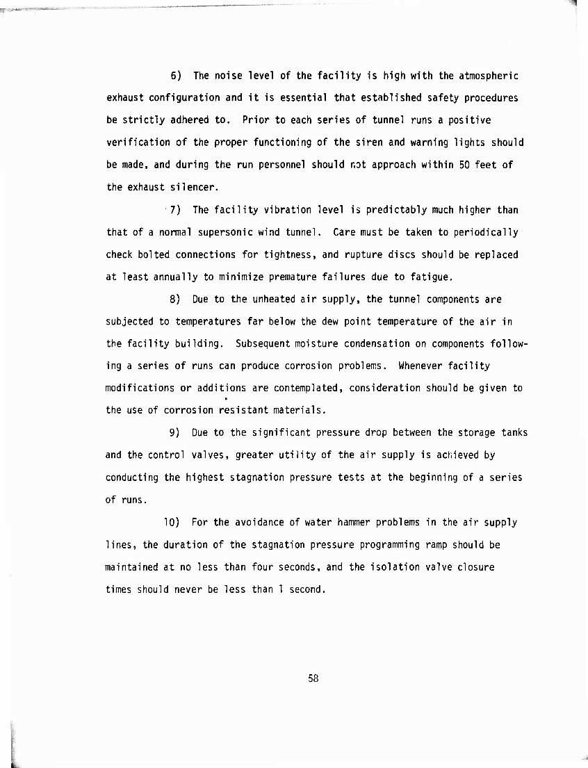
■
1
6) The noise level of the facility is high with the atmospheric
exhaust configuration and it is essential that established safety procedures
be strictly adhered to. Prior to each series of tunnel runs a positive
verification of the proper functioning of the siren and warning lights should
be made, and during the run personnel should not approach within 50 feet of
the exhaust silencer.
7) The facility vibration level is predictably much higher than
that of a normal supersonic wind tunnel. Care must be taken to periodically
check bolted connections for tightness, and rupture discs should be replaced
at least annually to minimize premature failures due to fatigue,
8) Due to the unheated air supply, the tunnel components are
subjected to temperatures far below the dew point temperature of the air in
the facility building. Subsequent moisture condensation on components follow-
ing a series of runs can produce corrosion problems. Whenever facility
modifications or additions are contemplated, consideration should be given to
the use of corrosion resistant materials.
9) Due to the significant pressure drop between the storage tanks
and the control valves, greater utility of the air supply is achieved by
conducting the highest stagnation pressure tests at the beginning of a series
of runs.
10) For the avoidance of water hammer problems in the air supply
lines, the duration of the stagnation pressure programming ramp should be
maintained at no less than four seconds, and the isolation valve closure
times should never be less than 1 second.
58

11) Closed circuit television should be used to view the test
section windows to insure that no accident occurs as a result of windows
cracking due to thermal effects during a run.
For those who may be involved with the design or operation of a similar
facility, it may be worth noting that the conveyance and control of high
density air at high flow rates and high expansion rates requires a close
examination of conventional design assumptions and practices. In the present
case it was found that the possibilities for water hammer problems, air
condensation problems and low temperature brittle fracture problems were
much greater than expected and other more conventional problems such as noise,
vibration and mechanical stresses were seriously intensified.
59

REFERENCES
1. "AFSC Technical Facility Capability Key," AFSCP 80-3, Air Force Systems Command, 1 July 1965.
2. Schaefer, W. T., Jr., "Characteristics of Major Active Wind Tunnels at the Langley Research Center," NASA TM X-1130, July 1965.
3. "A Compilation of Major Hypersonic Wind Tunnels in the United States," The Boeing Company Document No. D2-5785,
4. "National Wind Tunnel Summary," DOD-NASA, July 1961.
5. Test Facilities Handbook, Vol. 1, Arnold Engineering Development Center, July 1961.
6. "STA Wind Tunnel Listing," Supersonic Tunnel Association, 1966.
7. West, J. E. and Korkegi, R. H., "Interaction in the Corner of Intersecting Wedges at a Mach Number of 3 and High Reynolds Numbers," ARL 71-0241, AD734 540, October 1971.
8. "ASME Boiler and Pressure Vessel Code, Section VIII, Unfired Pressure Vessels," American Society of Mechanical Engineers, 1965.
9. Ferri, A. and Bogdonoff, S. M., "Design and Operation of Intermittent Supersonic Wind Tunnels," AGARDograph No. 1, Advisory Group for Aeronautical Research and Development, May 1954.
10. Azzouz, D. and Pratt, N. H., "Supersonic Turbulent Mixing, Part II, Design and Construction of a Mach 3 Blow-down Wind Tunnel and Its Instrumenta- tion," AASU Rept. No. 282, University of Southampton, May 1968.
11. Pope, A. and Goin, K. L., High-Speed Wind Tunnel Testing, John Wiley and Sons, Inc., 1965.
12. Haugen, R. L.; Moore, D. G. and Wennerstrom, A. J., "Velocity Profile Measurements in a Model Settling Chamber," Internal ARL Paper (available upon request), April 1969.
13. Friedrichs, K. 0., "Theoretical Studies on the Flow Through Nozzles and Related Problems," Applied Mathematics Group AMG-NYU No. 43, Applied Mathematics Panel 82.1R, New York University, April 1944.
14. Nilson, E., "Analytic Correction of a Two-Dimensional Nozzle for Uniform Exhaust Flow," Meteor Rept UAC-15, United Aircraft Corporation Research Dept., January 1948.
15. Baron, J. R., "Analytic Design of a Family of Supersonic Nozzles by the Friedrichs Method," WADC Technical Rept 54-279, AD 55 902, Naval Supersonic Laboratory, MIT, June 1954.
60

16. Burke, A. F., "Turbulent Boundary Layers on Highly Cooled Surfaces at High Mach Numbers," AFASD TR 61-645, ASD Symposium on Aerothermoelasticity, Dayton, Ohio, 1961.
17. Giles, Ronald V., "Fluid Mechanics and Hydraulics," Schaum Publishing Co., 1962.
18. Nagamatsu, H. T.; Sheer, R. E. and Graber, B. C, "Hypersonic Laminar Boundary-Layer Transition on 8-Foot-Long, 10 Cone, M] = 9.1 - 16," AIAA Journal. Vol. 5, No. 7, pp. 1245-1251, July 1967.
19. Pate, S. R., "Measurements and Correlations of Transition Reynolds Numbers on Sharp Slender Cones at High Speeds," AIAA Journal, Vol. 9, No. 6, pp. 1082-1090, June 1971. ~ ^
20. Wegener, P., "On the Experimental Investigation of Hypersonic Flow," Naval Ordnance Laboratory Rept. No. 9629, 1948,
21. Schueler, C. J., "An Investigation of Model Blockage for Wind Tunnels at Mach Numbers 1.5 to 19.5," AEDC TN 59-165, 1960.
61

62

800
Q
CO Q- 600 Q. <
z a. a.
z 400 Q. O cc
1000 PSIA 1400 PSIA 1800 PSIA 2200 PSIA 2600 PSIA
LJ cr (/) CO ÜJ cr Q.
200
100 MASS FLOW. m(LBm/SEC.)
200
Figure 2. Estimated Pressure Drop in Distribution Piping as a Function of Mass Flow and Storage Pressure
63

' - ' ^
1 1 «0
mm N «Mi (M ro Ö "'s -i
z a:
X
fO u> ^■
O
■ Ö 1
: o o _l Q ^^ II ^~ ^ X II >»
o oo CM
n
CM
CO CM
u CO
x-i
m -i 60
ii
O m x «o
c o
•r- +J
J-
Dl ■i— >+- C o
<_)
0)
N N O
CO
•5
ro 0)
O)
64

•^^MrWWFRWWWT^wrr^r-
1 DIA
.
ME
TA
L
)
BU
TT
ER
FL
Y
:L V
AL
VE
)
^^
14-I
N.
D
IA.
R
UB
BE
R
SE
AT
ED
BU
TT
ER
FL
Y
*
VA
LVE
(V
EN
T
VA
LV
E)
\-3
6-I
N.
D
IA.
CO
RN
ER
T
EE
WIT
H
MO
DE
L C
AT
CH
ER
z UJ UJ z
1^5 = E
■2
"J- - *1 \?=l r ICK
' -<< INi ̂
Ü 2 2
f
7 8-I
N.
DIA
. R
UP
TU
RE D
ISC —
N
AN
D
SL
IP
JO
INT
1
TIC
AL
R
UN
OF
3
6-I
N.
PIP
E
WIT
H
E
XP
AN
SIO
N
JTS
A
ND
T
IES
■ 20-I
N.
D
IA.
R
UP
TU
RE
^^
36-I
N.
D
IA.
RU
BB
ER
S
EA
TE
D
BU
TT
ER
FL
Y
VA
LV
E
(SP
HE
RE
VA
LV
E)
>
=c=
o •r- ■•->
s.
en •r— 4- C o
E 0)
+-> CO >>
on
4-> lO 3 fO
1 I o < 2
j J
I
)
1<
1
1
"T"
IB^B -VE
R
DIA
.
JOII*
r
~^ U "
UJ
C
* ■—fc. M il O
s^ o 0) C71
UI
65
k

CO Q.
UJ OC UJ
Q. CO
fO I- u.
o o o O o
UJ a:
UJ
Q.
200 300
ACCUMULATIVE RUN TIME, (SECS)
Figure 5. Rise of Sphere Pressure with Run Time for a Range of Stagnation Pressures
66

^ ■■ ■ ^ ■-■l"»-'
MACH 6 TUNNEL J (REF.) |
SPHERE (REF.)
EXHAUST PLENUM. GUIDE VANE ASSEMBLY AND SILENCER UNITS
i I i i "
SPACER REPLACING TUNNEL VALVE
MOPSIG RUPTURE DISC ASSEMBLY REPLACING VENT VALVE
RELOCATED CORNER TEE WITH MODEL
CATCHER
EXHAUST VALVE (RELOCATED SPHERE VALVE)
Figure 6. Present Exhaust System Configuration-Atmospheric
67

0 o ir H UJ (O I 3 o. < ^ x
is
U) 0) <J O s- a.
CO
ai s- en
68

— .• I.V ■ ■)- >. >'*,' ,■■ .»..I..)1*W.«*WWIPJ-™ «^^v-.^.•rsrr^.TSWH» U W-mi.^p»U^npn. ..
o UJ (0 O -i U
o
en UJ
3
O I- o
-I o K I-
o Ü
A
c > c o o
2
o en o
00
t/>
5 I/O
>
o
o o
en
QJ s- 3 en
< 03 O
o o UJ Ul (0 (0 o o -J -1 o Ü
UJ UJ > > -1 -J < 4 > >
-I -J o o cc cc H H z z o o Ü Ü
z I Ü u
CM tf)
69

PJ .i 3
a o
en O
O
+-> c o
t_)
>
o en
s-
= a.
70

T ■
z ZJ
UJ 12 Q.W Ü?
o i u. 4z «i Tu oT 0. -I IO ü|
1 »- So UJ
x < x > UJ
p Ü
r i ► T u •r— L ^^^^ cn
S^ ^Vw ^^^^ ^ *,. o u X X ^r x _l
en / \ / ^ \
o / 1 g \ o _i ■ ' J J_
■M ^: c (J J -L o o > r^s. / ■ ^v <_J
■M c i ^ (^ \
> r—
»—( >• c . -M 3 00 a: 3
f— UJ <— <u i , u o o CSI 3 0 UJ Ul
1
»r- UJ 0) (0 (U U. (n o o o 3
o -I -1 Ul en -J ! ü Ü (n Ll_ ü
— w o -j
UJ > i * If o -j
^ UJ UJ <n > 33 UJ
> s l_ i < < -j
UJ O) | - > > ^ W 3 2 > o < . ' UJ z z
a • -» x :. o- o ö -i s ü v uj o — — o UJ o < < cc Q. 1- -1 1- ^ ^
•
c O 2
(0 s
O 2 *2 o
Ü
71

2 <
(J
o
03
<
i.
72

UJ > 5
i is tu < v> >
tr O UJ
*§ <
CO CC UJ -I -I o oc (- z o o
E
■•->
o s-
+-> c
5 OJ s-
CO
ai s- a.
(O
oo
^ en
=! X
CC UJ 2 s < tr
o tr a.
73
^

TW-JMiW."""" ■ 'rr i inijupi » ,
in w tu o QL
ui > _i < >
o !5 3 »- O <
cr LÜ
So:
o
Lü
O <r y- z o o
ua + V)
0- Q. r 1^
x \ J i
. < + K- (/>
^ ^
,
■^T*» 1
4
^^ ' ^* 3
(M 1 ^
+ w
o o
o s.
+-> c o o
00 01 QJ u o s.
Q.
n
s. en
UJ
< oc o o a: a
74

O ! z
o N. > o 0} 1
• fs
1 * o
11 K.
2 Q II 1
3 x: •> 1 oc u •c <
a
r»
(M
I
00S OOh
IS > 2 *-• u (O (/} Ul 5- a w £i -J u O I c
■r—
UJ 3C
1 CM
»-« 1 1-
+-> l^
<u H-
<U (/) c o Q- (^ <U a: O) >
i—
w >•
(0 i.O z z III
0)
3 &. en
VISd
OOIE
i—
)09
0062 00it2 00S2 00E2 VISd
0012
s
03S 02S a.
08h 04ih OOh
£ 2 SilOA - (NOUISOd 3AnVA) dA
75

l ijHjupmKiimiiniiij
o »-
UI z -J v. a a
(A > m
• (Ni • IM to
u> i OB u» rt n ^^ 2 a 11
II
3 x: fc oe a •C <
a. d
n
005
OJ > to z > •-I u to UJ x: a V)
o u i
UJ s:
to
»-• +J H CO
CD H-
O) CO
fj
co
ä > (D
(D
ooe ooz VISJ - 0d
oorc 0042 00^2 00S2 VISd - SJ
00C2
C 2 SilOA - (NOUISOd 3A1VA; «JA
00T2
1 ,.. ■
003 i—
oss -^ 1— ..i
02S - »i
1
08t) '0i
i— i
Ohh __j —j
00
,__ —j— -t. —1— L. __l , —_t__ 1 . - „J
76

'•'■•!*'«»•.■«. -.
u 1- UJ z ~J w a N. >• o
x: A a
• en ^ (A i •
L ii
•
2 a u n Z3 £ «. ex. O « <
-
id a. a. o > a.
oos 001» 00E 002 VISd - "4
ooie 0062 00/2 00S2 00C2
to
U)
ai >
u to >
en 1 u c UJ •1"
s CM »-« 1- 1
+-> (/I a> i-
CJ <u
o S-
o o *-*
CO
10 O) z e »-I 3 z en w Ll- a.
o Q
0012 VlSd
003 03S 02S 08h Ohh 00h
e 2 SilOA - {NOUISOd 3AnVA) dA
77

o a.
10
00S
U)
- :r
0)
o > UI (0 U) >
-C n 1
UI •n-
x: 1 •-• MJ
h- 1
■(->
I— ra OJ
o s-
+-> c o o
•-• en
(3 Z ID
*■* -1 z O) UI •r—
a. U.
o o 00C 002
VISd - 0d
OOtE 0042 00^2 00S2 VISd - 'd
ooe2 0012
009 035 025 08h Ohh 00h
t 2 SilOA - (NOUISOd 3A1VA) dA
78

o 00
■o c
o
en c •r-
£ a a> CO o
O0
o CM
s_
en
79

t— 1 ^
0 I 2 SCALE IN INCHES
A. RAKE SIDE VIEW
B. RAKE PLAN VIEW
Figure 21. Scale Drawing of Mach Number Survey Rakt
80

'
J- 3
4->
o c
c
<c 0) o c <u s- 0)
o;
QJ
a:
> s- 3 (/I
CM CM
£ CT
a
si

O - CALCULATED FROM RAKE PITOT PRESSURES
• - CALCULATED FROM WALL STATIC PRESSURES
O - CALCULATED FROM ^ PITOT AND STATIC PRESSURES
-4
-4
-4
"T"
-Gu ■o-
"T"
-G- B.oX-
"T"
-o-
*%/l' 21.61 X I06ft; 2.9 ■
-3 -2
—r
2.8
4> - 0* J.
-T M«
3.01 £1 _a.
•fi
—r
® 2.9 + R,//-22.44 X lO6^'1
! 2.8 2S. X
£L
</> • 45
-3
—r
-2
—r
♦ i
T
Rf/i. X
XIO6^'
-3
—r
-2 -I
-M
3.0
2.9
-2.8
$ • 90*
+ 1
iD-
gy/i- 21.5 6 X 10 6 ft.
4 A~ 3 - 2
WEST WALLl
-I
.a <^ • 135*
+ 1
y/AS
0
X ♦ 2
—r
"O"
♦ 2
♦ 2
—r
"Ö"
2%
X + 3
—r
♦ 4
i 2%
T- i2u
•►3 -»• 4
2%
X •►3
—r -►4
1 2%
ü ♦ 2 +3 t **
I EAST WALL
Figure 23a. Impact Mach Number versus y/As for xp/xr - 0.690 at p0 = 109 psia and T0 = 430oR
82

■
0 - CALCULATED FROM RAKE PITOT PRESSURES
• " CALCULATED FROM WALL STATIC PRESSURES
9 - CALCULATED FROM C PITOT AND STATIC PRESSURES
-4
-4
-4
-4
XT -r ■O
—r IK
«..-•
3
2.9
"T-
■o
R.//" 1993 X 10•ft -L I L -3
—r -2
—r -i
2.8 4> • 0*
±
M
O -GT
O
Rt/i- 21.09 X I06ft' r i i
-3 -2
-r -i
3.0
2.9-fr
•2.8
4-1
T-
^> • 45*
3.0S 0
_Q ^3.
2.9 + R,//- 20.48 X lO6«.'1
JS i ! 2.8 -2
-o- o
S^H
WEST WALL)
-I
♦ I
—r
0
<^ • 90* ±
+ 1
-o-
Rt//- 21.8 8 X 10* ft."' ^^ " '35* 2.8
0
y/AS
+ i
"T"
JL •»•2
—r
0
i ♦ 2
—r
TDr
i. ♦ 2
—r
O
2%
"T-l ±
♦ 3
—r ♦ 4
i_. o_|%
I ♦ 3
—r ♦ 4
"2%
JSL + 3
—r
♦ 4
__t 0 2%
T- 4-2 +3 A 4-4
I EAST WALLl ö
Figure 23b. Impact Mach Number versus y/As for xp/xr - 0.345 at p0 - 111 psia and T0 = 4770R
83

O - CALCULATED FROM RAKE PITOT PRESSURES
• - CALCULATED FROM WALL STATIC PRESSURES
O - CALCULATED FROM C PITOT AND STATIC PRESSURES
-4
-4
-4
-4
-r T
o
M? r" i.oi o-
Rt/i« 21.58 X 10St,'1
3
2.9
-3
—r
-2 2.8
^> • 0* J.
G O- 3.oA.
2.9--
■0-
R9/I' 21.13 X I06ft"1
J 1 1 2.8 -3 -2
T
</> • 45*
♦ I
-o Q 3.0W
"T"
o «.//• 20.32 X I06ft." -j! I L-
2.9--
-3 —r
-? -1
o "cr
-2.8
M
3.0
4> - 90'
+ 1
O 29 , ,
R./i- 18.21 X lO6^ I 9 " '35 . I ' ' 2.8 A-3 - 2 " I C? + I
WEST WALL
V AS
T"
± + 2
—r
-0-
± + 2
—r
■O-
+ 2
—r ■O
■f 2
T
■^■
±
i. 2%
T ■»- 3
—r •► 4
i "GT 2%
± •►3
—r + 4
_LJ — 2%
± •»•3
—r
+ 4
O 2%
T- lU. + 4
EAST WALL
Figure 23c. Impact Mach Number versus y/As for xp/xr 0 at p0 = 111 psia and T0 = 484
0R
84

O - CALCULATED FROM RAKE PITOT PRESSURES
• - CALCULATED FROM WALL STATIC PRESSURES
<1 - CALCULATED FROM £ PITOT AND STATIC PRESSURES
-4
-4
-4
T T
-nr o
,6^-1
3.00
2.9 • Rt/^- 20.78 X 10° ft. j 1 1 2iQ,
-3
—r
-2
—r
-O-
M
3.0
O "S" I
Rt/i- 21.12 X lO6^"1
I I \ -3 -2
2.9 +
•2.8
6 ,.-1 R./i- 20.05X I06ft _li l L_
2.9-
-3
—r -2 -i
T
•2.8
-M
3.0 -o- "0"
-O-
4> - o*
■xzr
^) • 45
-. r-Mr r
■X3 O —Ä 0-
<j> • 90*
+ 1
2.9 R./i" 2 0.34Xl06ft.'i 9-135
■ I I I 2.84 L
A-3 -2 -I 0 +
WEST WALL
v/ AS
T
"Gr
-L + 2
—r
X + 2
—r
•o-
+ 2
—r
+ 2
o i 2 V. T J
± -»• 3
—r ■f 4
i o 2%
+ 3 + 4
T + 3
—r ■♦•4
i 2 V.
O
♦ 3 I + 4
EAST WALL
Figure 23d. Impact Mach Number versus y/As for xp/xr + 0.345 at p0 = 108 psia and TQ = 4770R
85

O - CALCULATED FROM RAKE PITOT PRESSURES
• - CALCULATED FROM WALL STATIC PRESSURES
9 - CALCULATED FROM £ PITOT AND STATIC PRESSURES
-4
-4
-4
-4
T
t-r
H,//' 1905 X 10St
-I My
Q 3oi T"
-i 2.9-
-3
—r -2
—r -i
2.8 4> ' 0*
± + 1
-o- ■o- 0
MI R9/I' 20.36 X lO6^'
I I L_
2.9-•
-3
—r -2 -I
•2.8
o </> • 45*
♦ I
© -O- e hpi 2.9 f
R,//- 20.30 X 106ft.■,
' ' 1 2.8
¥ 4> • 90*
-3
—T
-2
—r -i
M
—O- 3.0
—T
75 ^~2.9
R,//' 20.45 XIO0«."1
-2.8
A o
4> - I35#
t-3 , -2
|WEST WALLj
-I
y/AS
T
J. ♦ 2
—r
■O-
X ♦ 2
—r
^e- j.
♦ 2
—r
■o-
_L. 2% r-
± •*- 3
—r ♦ 4
^L '2%
T-l i
•f3
$
♦ 4
2%
X ♦ 3
—r 4-4
JL. -0- 2%
T- ♦2 +31^4
I EAST WALLl
Figure 23e. Impact Mach Number versus y/As for xp/xr + 0.690 at p0 = 103 psia and T0 = 472
0R
86

O - CALCULATED FROM RAKE PITOT PRESSURES
• - CALCULATED FROM WALL STATIC PRESSURES
3 - CALCULATED FROM £ PITOT AND STATIC PRESSURES
-4
-4
-4
-4
-©_
-r
-o-
-1 M^
-O ioi
6^-1 2.9'
R«/i" 60.61 X lO^ft
-3
—r -2
—r -i
2.8
Q 2.9-- R./i- 61.7 3 X I06ft',
& 1 1 2.8 -3
—r -2
—r -i
T
v* X 10 6 ft.*1
-3
—r -2
-M
3.0
2.9
•2.8
M
3.0-- —6
o R./i" 59.48 X I06ft 6 M*-*
2.9--
I - 2 -1—2.8
-I
WEST WALL
4> - o* ±
4> ' A5'
+ 1
4> ■ 135*
0
y/AS
-r O
± + 2
—r
•»•2
T^
♦ 2
^4_- 2%
T x
♦ 3
—r ♦ 4
i 2%
T JX
-»•3 + 4
1 1 I I
4- 2% |
JL + \ <f) > 90*
• i
0 +1 + 2 + 3 + 4
2%
—?T * 4
EAST WALL
Figure 24a. Impact Mach Number versus y/As for xp/xr - 0.690 at p0 = 306 psia and T0 = 468
0R
87

O - CALCULATED FROM RAKE PITOT PRESSURES
• - CALCULATED FROM WALL STATIC PRESSURES
9 - CALCULATED FROM £ PITOT AND STATIC PRESSURES
.4
-4
-4
Rt/^- 57.69 X K^ft"' -£- I I -3
O
*.//■ 56-27 XIO6«.'1 Qi ' 1 2.8 -3
—r -2 -I
O 2.9 + Rt//" 59.90 XIO6«."1
■ I I I 2.6
WEST WALL
Figure 24b. Impact Mach Number versus y/As for xp/xr - 0.345 at Po = 316 psia and T0 = 4820R
88

O - CALCULATED FROM RAKE PITOT PRESSURES • - CALCULATED FROM WALL STATIC PRESSURES 9 - CALCULATED FROM £ PITOT AND STATIC PRESSURES
•»-2 +3 f *'4
I EAST WALL
Figure 24c. Impact Mach Number versus y/As for xp/xr 0 at Po = 323 psia and T0 = 4910R
89

O - CALCULATED FROM RAKE PITOT PRESSURES
• - CALCULATED FROM WALL STATIC PRESSURES
O - CALCULATED FROM £ PITOT AND STATIC PRESSURES
-4
-4
-4
-4
—r
-o-
—r
■GT 3.00
6^-1 2.9-
Rt/i- 58.61 X 10° ft. I I I
-3
—r -2
—r
-O- 0 ü
R,/^" 59.38 X lO6^1
-J I L_ -3 -2
•2.8
M
3.0
29:
•2.8
—r
-o-
<j> ■ 0* J.
■f I
—r
-O-
<f> . 45*
♦ I
■O -O- 3.0;
*m/lm 57.14 X ID6»."1 <^ • 90* I I 1 2.8-1 1
-3
—r -2
—T
-I + 1
-M
3.0
—r
O
I O 2.9
*%/lm 57.09 X l06ft.H | 9 ^ 2.8
135
-3 - 2 -I
WEST WALL
-r
JL •»■2
—r
-Q-
X ♦ 2
—r
O
♦ 2
-►2
J. ♦ 3
—r
± + 3
—r
"O"
J. ■f 3
—r
i 2%
T + 4
2%
•f 4
1 2%
+ 4
i 2%
0 ♦!
y/AS
Figure 24d, Impact Mach Number versus y/As for xp/xr = + 0.345 at p0 = 313 psia and T0 = 4830R
+ 3
EAST WALL
90

O - CALCULATED FROM RAKE PITÖT PRESSURES
• - CALCULATED FROM WALL STATIC PRESSURES
9 - CALCULATED FROM £ PITOT AND STATIC PRESSURES
-4
-4
-4
-4
1 ' ■T ■ I
O vy
1 V^' 59.76 X io« ft;1
L . -3 -2
—r -i
^L
P,//" 59.2 2 X I06ft 6#.-l
-3
—y
-2
—T
•2.8 <j> . 45*
♦ I
J2- .0. G
6 ,.-1
"I 3.0Ä
2.9-• R./i- 61.09 X 10* ft.* t 1 1 2.8
O
<f> • 90*
-3
—T
-2 -I
M
3.0 I ♦ 1
—r
O , 2 9 + Rt/i" 61.47 X 10* ft."*
WEST WALTI
-I -2.8
O
(p " 135*
0
y/AS
+ i
± ♦ 2
—r
-o-
J. >2
—r
i. ♦ 3
—r ♦ 4
-G I— - 2%
T-l X
♦ 3
—r ♦ 4
■&- 2%
♦2 ♦31 +4
lEAST WALL)
Figure 24e. Impact Mach Number versus y/As for xp/xr + 0.690 at p0 = 318 psia and T0 = 4760R
91

O - CALCULATED FROM RAKE PITOT PRESSURES
• - CALCULATED FROM WALL STATIC PRESSURES
3 - CALCULATED FROM £ PITOT AND STATIC PRESSURES
-4
-4
. 4
sx -1 M*
6 „.-1 2 9-
R,//- 97.78 X 10* ft. J.
-3
—r -2
—r
2.8
■O"
O 2.9 + R./i-99.43 X lO6/!"'
■2.8 ♦ -^ -2 -1
1 i i
-
yi- —i- X 10 St.'1
1
M
-3
—r -2
3.0--
2.9-■
2.8
"T"
<t> • o#
JL ■fl
-T
■o-
<^ ■ 45#
+ 1
</> • 90*
♦ I
R,/i" 96.27 X I06ft
3 -3 - 2 .2.8
0. - 135*
WEST WALL
0
y/AS
■f i
¥
i
♦ 2
—r
iD-
J. ♦ 2
—r
-^2
-i M m 1 r
^ 3 0i O fS o O-
♦ 2
i3L i 2%
"T J
X ♦ 3
—r ♦ 4
i - 2%
Tt
i-J 2%
J. •»■3
—r f 4
2% r •f 4
EAST WALL
Figure 25a. Impact Mach Number versus y/As for xp/xr - 0,690 at p0 = 518 psia and T0 = 4780R
92

O - CALCULATED FROM RAKE PITOT PRESSURES
• - CALCULATED FROM WALL STATIC PRESSURES
9 - CALCULATED FROM £ PITOT AND STATIC PRESSURES
-4
-4
-4
-4
—r -0-
-1 Mr -C —Ö
3.0*
-r
R./^' 88.95 X lC€ff, 2.9-
-3
—r -2
—r -I
-2.8 <f> - o*
X ♦ I
T
G "O"
Ms-
3.0&-
"t/i" 93.00 X lO6^1
-J! i i -3
-T
-2
—r
O—3
2.9+
2.8
"T"
O
-I
if) - 45* 1
T "I 3.0ft-
♦ I
—r
O 3.
2.9 +
0
R,//-90.01 X \06U'i
Jff 1 I 2.8 <f> - 90*
J. -3
—r
-2
"Ü"
-I
-X2L
•n M
3.0 I Q 2.9-- Rt/^" 97.04 XiO6«."1
t-3 , -2
|WEST WAITI
-2.6 4> • 135*
0
y/AS
+1
-T-
•»-2
—r
G
i
♦ 2
—r
"GT
+ 2
—r
0
+ 2
2%
J. ••»• 3
—r ♦ 4
_J_J
L
♦ 3
—r •► 4
_L. 2%
0 -L.
+ 3 + 4
i 0
2%
T + 3 I + 4
EAST WALL
Figure 25b. Impact Mach Number versus y/As for xp/xr - 0.345 at po = 520 psia and T0 = 4910R
93

O - CALCULATED FROM RAKE PITOT PRESSURES
• - CALCULATED FROM WALL STATIC PRESSURES
O - CALCULATED FROM £ PITOT AND STATIC PRESSURES
-4
T
o
R,//" 95.73 X 10* ft
"T" -~r
2.9-
R9/l' 92.78 X I06fr. I I » —I 2.8 ITS Tg^ -I
WEST WALTI
0 4-1
y/AS
-o- i 2%
■f 2 "f3T + 4
|EAST WALL
Figure 25c. Impact Mach Number versus y/As for xp/xr = 0 at Po = 532 psia and T0 = 4990R
94

O - CALCULATED FROM RAKE PITOT PRESSURES • - CALCULATED FROM WALL STATIC PRESSURES 9 - CALCULATED FROM £ PITOT AND STATIC PRESSURES
-4
-4
-4
-4
i ■ ■ -r- n
0 o Ü
Rt/i« 93.94 X ID6 ft.'1
-3
—r -2
—r
R9/l' 95.2 5 X I06ft. -I 29:
-3
—r -2
-2.8
M
3.0
^> • 45*
■XT 2.9
«./,/• 92.62 X 106 ft.'1 \ $ ' SO* Jl 1 1 2.8 J 1
-3
—r -2
—T
-I
3.0
"T"
-O- -^ 0
O 2.9 Rt/i'92.38 X 106ft.H 19 -135
-_j 1 1 2.8-i L
WEST WALL y/AS
± + 2
—r
± -»■2
—r
-o-
•»- 2
T- 4 3 + 4
i o 2'/.
T + 3
—r 4 4
J... — 2%
+ 3 I 4 4
EAST WALL
Figure 25cl. Impact.Mach Number versus y/As for xp/xr + 0.345 at p0 = 517 psia and T0 = 4910R
95

O - CALCULATED FROM RAKE PITOT PRESSURES
• " CALCULATED FROM WALL STATIC PRESSURES
O - CALCULATED FROM £ PITOT AND STATIC PRESSURES
-4
-4
-4
-4
T —r
-o-
M
6- .3.0j
2.9-• Rt/i- 9 6.19 X ID6 ft."1
J 1 1 2.8,
"T
-o
4> - o* -3
—r -2
—r
o
R,/i- 93.64 X lO6^'1
-J I I
I MA
2.9--
-3
—r -2 -I
•2.8
M
O
</) - 45*
•H
o o 6^-1
Ö-
Rt/i- 97.43 X I06fr.'
3.0
2.9 +
-3
—r -2 -i
-2.8 <^ ■ 90*
+ 1
3. -O- 4
*•/!' &7.0I X 10 ö ft S-.H 2.9-
E - 2 •2.8
O
$ ■ 135*
WEST WALL
0
y/AS
T
_L + 2 —r
-O-
± + 2
—r
-o-
+ 2
—r
^x.
+ 2
T 0_L
2%
+ 3
—r
± ♦ 3
—r 0
± + 3
—r
-»- 4
i 2%
T + 4
1 2%
T 4 4
^_ 2%
T + 3 I + 4
EAST WALL
Figure 25e. Impact Mach Number versus y/As for xp/xr + 0.690 at p0 = 523 psia and T0 = 4860R
96

T i
/ /
/ /
o / /
/ /
/
/
3.06
3.04 ■-
a:
2 v
<I
z
¥ 00 ■ - ^^r-
2 98--
Ui 2 96
^ 2.94--
2.92 --
i. 2.90-
OESIGN MACH NUMBER
THR\?"[ -FAIRED THR"Ü» DATA
SYM. i ^ — I DEC 0 0 9 45 0 9 0 A 13 5
-L 1.0 -0.8 -0.6 -0.4 -0.2 0 0.2 0.4 06 0.8
*
Xp/XR
o
Figure 26a. Center!ine Mach Number versus Longitudinal Distance for po = 100 psia, To = 4680R, where Re/£ = 20.69 x 10⁶ per foot
97

. i T i %
o o
3.06
3.04-
T - /
- /
- /
i u <I
Ui z
3.00 ■-
2.98 --
fit ^ 2.96 z Ui o
2.94-
2.92-
^-2.90-
■OESIGN MACH NUMBER
-e^r
-FAIRED THRU DATA
SYM. fi </> 1 DEG. O 0 9 45 0 9 0 ^ 135
X -L JL 1.0 -0.8 -0.6 -0.4 -0.2 0 0.2 0.4 0.6 0.8 1.0
Xp/XR
Figure 26b. Centerline Mach Number versus Longitudinal Distance for po 300 psia, T0 = 480.06oR, where Re/£ = 59.2 x 10⁶ per foot
98

T i ^
1 a
3.06
304-
tt ui
3N Q
I i u <
UJ
roo
2.98 -
/ a: w 2.96 z UJ o • 2.94
2.92 -
2.90-
0ESI6N MACH NUMBER
^ O
FAIRED THRU DATA 2 SYM. i <t> — IDE
if G. 0
AS. 90
13 5
± JL 1
■1.0 -0.8 -06 0.4 -0.2 0 0.2 0.4 0.6 0.8 1.0
Xp/Xp
Figure 26c. Centerline Mach Number versus Longitudinal Distance for p0 500 psia, T0 = 489.05oR where Re/£ = 95.0 x 10⁶ per foot
99
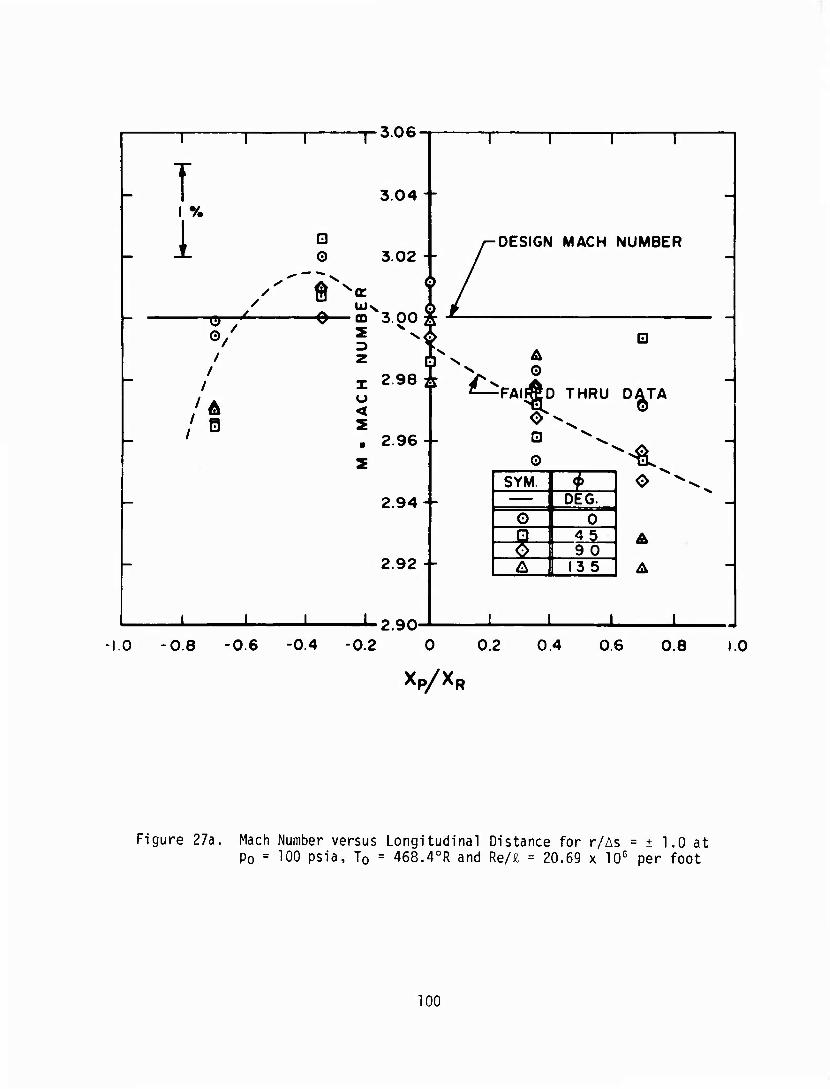
T I ^
1 0
306
3 04-
3.02 -
/ fi sa:
DESIGN MACH NUMBER
■0—00 3.00
3
x 298 o <
. 2 96 +
CD
2.94--
2.92 -
J. ± 2.90-
Ä
^ 0 ■FAI ÄD THRU DATA
o ^^
"-1 SYM. * o
DEG. 0 0
5 45 A ? 90 A 13 5 A
-L J. 0 -0.8 -0.6 -0.4 -0.2 0 0.2 0.4 0.6 0.8
Xp/XR
Figure 27a. Mach Number versus Longitudinal Distance for r/As = + 1.0 at Po = 100 psia, To = 468.40R and Re/£ = 20.69 x 10⁶ per foot
100

3.06
T I t
i DESIGN MACH NUMBER
O
O
r /0
/ I
I <s>
'S
! 298-- ^
< Z , 2 96-
2.94--
2.92 -
I ^ L ± 2.90-
0
■FAIRED THRU DATA
IS SYM. || </> i DEC O 0 9 45 ? 90 AA 135
A
J. 1 1.0 -0.8 -0.6 -0.4 -0.2 0 0.2 0.4 0.6 0.8
Xp/XR
1.0
Figure 27b. Mach Number versus Longitudinal Distance for r/As = ± 1.0 at Po = 300 psia,T0 = 480.06oR and Re/£ = 59.2 x 10⁶ per foot
101

T0 3.06
T i
3.04 ■ ■
3.02 - -
Nt
•DESIGN MACH NUMBER
^ Wx 0 3.00
O/ 3
2 98 - -
/ /
/ /
x u <
• 2 96 4-
2.94 - -
2.92 - -
J. ■L2.90-
¥ S
0 O
•FAIRED THRU DATA
^^^ o
SYM. * DE6. O 0 e 45 ÖA 90
| A | 135 1
± ± 1.0 -0.8 -0.6 -0.4 -0.2 0 0.2 0.4 0.6 0.8
Xp/Xp
1.0
Figure 27c. Mach number versus longitudinal distance for r/As = ± 1.0 at Po = 500 psia, T0 = 489.05oR and Re/£ = 95.0 x 10⁶ per foot
102

T I %
1°
3.06
3.04-
OESIGN MACM NUMBER
/ /
/ 6 I
h / / /
< i G i ■^2.90-
^
2 94-
2.92 -
f-
SYM. 1 * 1 DEG. o t"~o~i ( ~Ö| TJ 45 o 1 90 ! A 1 i 135 1
± ± ± 0 -0.8 -0.6 -0.4 -0.2 0 0.2 0.4 0.6 0.8
Xp/XR
Figure 28a. Mach Number versus Longitudinal Distance for r/As = + 2.0 at p0 = 100 psia, T0 = 468.40R and Re/£ = 20.69 x 10⁶ per foot
103

T 1
3.06
3.04 -
DESIGN MACH NUMBER
/ a /
/ O
<
Q , 2 96 I O 5
FAIRED THRU DATA
t I
I I
h / /
/
i L
2.94--
2.92 --
± J. 2.90-
SYM. 1 </> — 1 DEG. 0 0 9 45 0 9 0 A 13 5
o i. J.
.0 -0.8 -0.6 -0.4 -0.2 0 0.2 0.4 0.6 0.8
Xp/XR
Figure 28b. Mach Number versus Longitudinal Distance for r/As = ± 2.0 at p0 = 300 psia, T0 = 480.06oR and Re/£ = 59.2 x 10⁶ per foot
104

T i •/
i ©
306
3.04-
3 02 -
O
Ul m 3.00
I 1
DESIGN MACH NUMBER
o
-o- ^"
o z __4> T—o Ö- o 0 ^-FAIRED THRU DAT^
/
/ /
_ / / /
i I Q—J.
<
Q , 2.96--
^ 2 94 0-
2.92 -
DATA Ä
± ± 2.90-
SYM. * DEC
O 0 9 45 § 90 A 135
J 2± ± ± •10 -0.8 -0.6 -0.4 -0.2 0 0.2 0.4 0.6 0.8 1.0
Xp/Xp
Figure 28c. Mach Number versus Longitudinal Distance for r/As = ± 2.0 at Po = 500 psia, T0 = 489.05oR and Re/Z = 95.0 x 10⁶ per foot
105

i T 1
306
3.04 - -
. 2 96
JL 2.90- Ö
O
DESIGN MACH NUMBER
FAIRED THRU DATA
i SYM. * 294 A-
I O DEG.
0 D 45 O D 90
2.92- Ä 1 135
J. ±
Figure 29a. Mach Number versus Longitudinal Distance for r/As = + 3 0 at Po = 100 psia, TQ = 468.40R and Re/Z = 20.69 x 10⁶ per foot
10 -0.8 -0.6 -0.4 -0.2 0 0.2 0.4 0.6 0.8 1.0
Xp/XR
106

306
T i
/ /
/
_ / /
/
_/ /
/
/
i o <
, 2.96--
2 94-t
2.92
-L2.90-
FAIRED THRU DATA
SYM. f DEC [
1 O 1 0 9 ! 4 5 5 ) 9 0
! A I 113 5
10 -08 -06 -04 -0.2 0 0.2 04 06 08 10
Xp/XR
Figure 29b. Mach Number versus Longitudinal Distance for r/As = ± 3.0 at p0 = 300 psia, T0 = 480.06oR and ReA = 59.2 x 10⁶ per foot
107
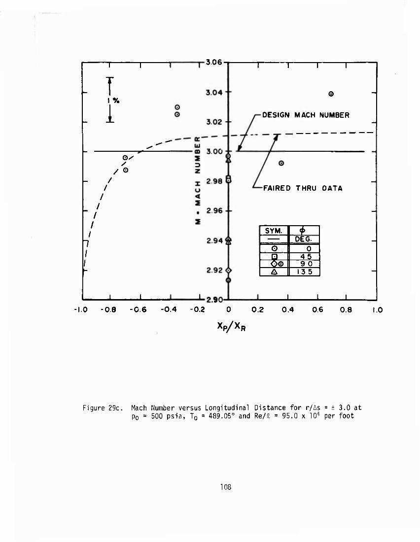
3.06
T i ^
1
s / 0
J. •2.90
0
DESIGN MACH NUMBER
FAIRED THRU DATA
SYM. | 4> 1 DEG. O 0 5? 45 6© 90 A 135
1 -L 1.0 -0.8 -0.6 -0.4 -0.2 0 0.2 0.4 0.6 0.8
Xp/XR
Figure 29c. Mach Number versus Longitudinal Distance for r/As = ± 3.0 at Po = 500 psia, TQ = 489.05° and Re/£ = 95.0 x 10⁶ per foot
108

- oio
<0
O ^^ T O o O
X — 0) m
1 <^- (Vl ID 0)
^
>- O □ 0 w
T o Q
< UJ Q: <
- 0)
o o t
OE X
ro
I
0) c c
h- J- 0)
I- 4J O 0)
»t- E fO
OJ s- O to C Q. (O
4-> fO to
•r- I/) O (O
r- S- <a a» C JQ
•r- £ -a 3
•i- 10 OITJ C r— 0 O
—I C
tn at </) ^ J: 0) 4-> > •!-
3 L. 01 c
XI o £•>- 3 +J Z T-
x: c u o
^^ r— Q. (0 E
o 00
OJ s. 3
109

IT k> (O o If) 0
X 0> * o * <r>\ S» <o ro o IO <o x] O
+ o 6
1 0 1
> 0 akJoy «n - - - J
o o
o 0)
o 00
o <0
o o u. a: HI a.
o x
o
+-> o o
s- ai Q-
S- 0)
E 3
•o O c >> OJ a:
00
0) > S-
E 3
o "3
ai s-
cr
(VJ 0
O O
CD «0 9»
* 9 0)
ro K) M N N N
O 00
10 c fO <u
4-> O O M O
• ro
O (1) t. 3 cn
110

O.IZ'X 45 CHAMFER
OTOT
A. WEDGE PLAN VIEW
1.00" 0.75"
B. WEDGE SIDE VIEW
Figure 32. Scale Drawing of Flow Angularity Wedge
111
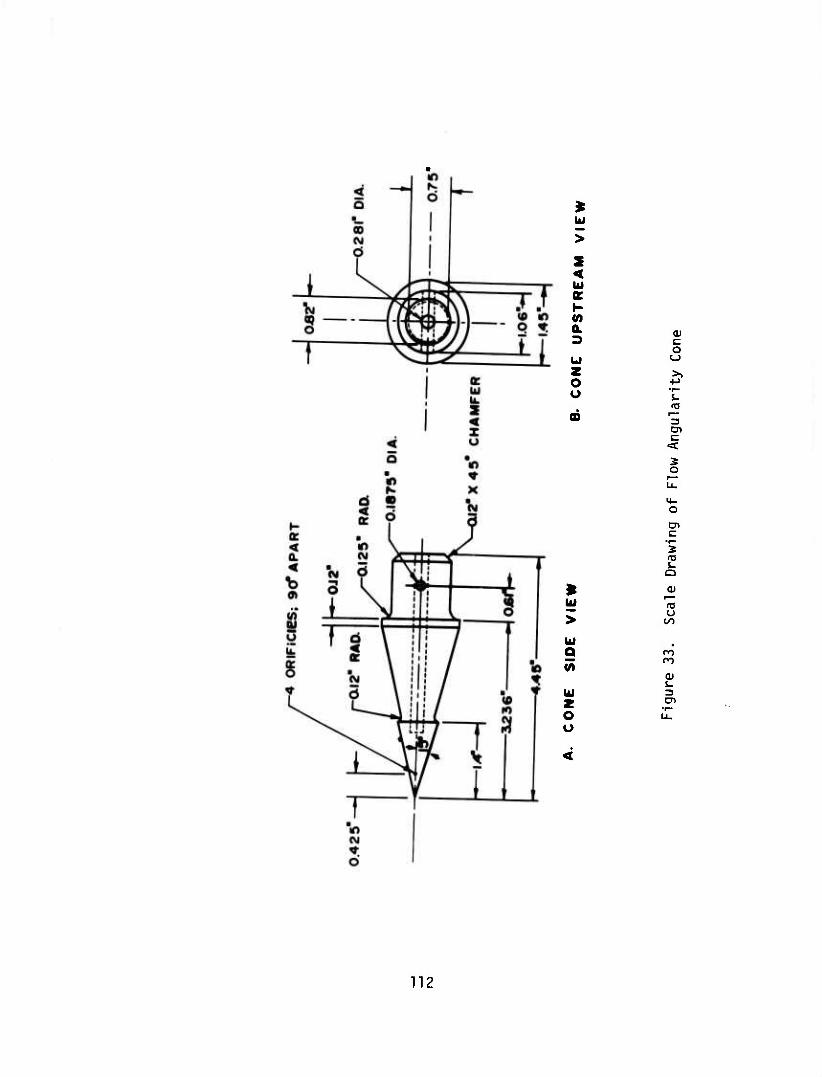
UJ
< tit It
tf) Q. 3
O o
CD
> bi Q
UJ z o u
c o
•r-
<T3
c < 3 o
4- O
Ol c
•f—
I (U
O 1/1
n
en
112

Figure 34a. Normalized Surface Pressure Difference versus Angle of Attack at xp/xr = - 0.690 for p0 = 103.6 psia with Settling rhamber Spreader Cone Tip Downstr&am
113

Figure 34b. Normalized Surface Pressure Difference versus Angle of Attack at xp/xr = - 0.345 for p0 = 100.6 psia with Settling Chamber Spreader Cone Tip Downstream
114

-1.6
A-UPRIGHT 0-INVERTED
L_
Figure 34c. Normalized Surface Pressure Difference versus Angle of Attack at xp/xr = 0 for p0 = 100.6 psia with Settling Chamber Spreader Cone Tip Downstream
115

Q IN DEGREES
A-UPRIGHT O-INVERTED
Figure 34d. Normalized Surface Pressure Difference versus Angle of Attack at xp/xr = 0.345 for p0 = 95.0 psia with Settling Chamber Spreader Cone Tip Downstream
116

Figure 34e. Normalized Surface Pressure Difference versus Angle of Attack at xp/xr = 0.690 for p0 = 95.4 psia with Stagnation Section Spreader Cone Tip Downstream
117

SPREADER CONE
± T
CASE A
TURBULENCE SCREENS
i --U
CASE B CASE
d2-*U
r/R
1.0
0.9
0.8
07
0.6 -
0.5 -
0.4 -
0.3
0.2
0.1
0
i—i—i—i—i—i—r
j i L
Figure 35. Velocity Profile in a Model Settling Chamber with and without a Spreader Cone
118

i 1 1 r- 0-2* WEDGE (0/2-10') Q-CONE (0/2« 15')
-0.4 - -
■0.8
M • 3.01 ffi ..-I Rt/i- 93.42 X IGT ft.
_J I I L
J -0.8
Figure 36. Flow Angularity versus Lateral Distance at xp/xr = 0 (Rhombus Center) with the Spreader Cone Tip Upstream
119

T
O - 2d WEDGE (d/2 ■ 10*) Q-CONE (9/2 - 15*)
0.8 8
-o
-F=^
0.4--
i r
I ü I oy=^F=s=f
-0.8
r©- O
-0.4 4- M-301 . -, Rt/i- 93.42 X ICTft.
JL J L
O
O
I 1 I 1
8
1 1 1 1 ■• 08- —
0
8 Q4 - -
0
I i i o In) I J-; I B i 1 t o
| ■ 0 < t O 1 P 1
_0 -0.4- - M - 3.00 Rjf-58.1« X IO*ff.H
-
1 1 1 -1 -1X8-1 1 1 1 1
WEST WALL
-D-
0.8
0.4--
..f
1 ol ho—l—o i -1.0 -0.8 -0.6 -0.4 -0.2
J 1 ., 0.8
CAST WALL
+-oH h 02 0.4 0.6 04 1.0
04 -L M - 2.99 R^i' 20.62 X 10* ft"*
± ± J L
Figure 37. Flow Angularity versus Lateral Distance at xp/xr = 0 (Rhombus Center) with the Spreader Cone Tip Downstream
120

SYMl M 20.62 58.18 93.42 20.62 58.18 93.42
WEDGE
-I 1 ' L-0.6
A. SPREADER CONE TIP UPSTREAM
1 1 0.6
WEST WALL 0.4 --
t7
8
T 1 r
EAST WALL
Q 0 0.2 -^
-ol h s •*&-
w o
■1.0 -0.8 -0.6 -0.4 -0.2 0 0.2 vv 0.4 0J6 OB I
-0.2 - -
-S I L -L-0.4
Z/(b/2) -*-
_L J L
B. SPREADER CONE TIP DOWNSTREAM
Figure 38. Unit Reynolds Number Effect on the Flow Angularity at xp/xr = 0 (Rhombus Center)
121

+ X^/)(R. -0.690
1 1 L
I r
—o
H H xyxR ■ -0.34 5
H f-
Wn'0
T r
G
+ + Xp/*n ' 0.3 4 5
I I L
/"
—I 1 WEST WALL O-
■f
1^0.4
- 8 n •0.4
PROBE
I
V4 -8 H Tt
■0.4
1 0.4
- 8 H 7t
-0.4
n .0.4 a -J -0.4
1 04 T
- 8 —
CONE
•1.0 -0.8 -0.6 -0» -0.2 | Xp/fr ■ 0.690
J -0.4
0.2
"Cr
4 0 Z/lb/2
B/2 ' 15*)
r E^T WALL A
6 0.8 1.0
Figure 39. Flow Angularity versus Lateral Distance with Longitudinal Distance as a Parameter for pn = 100 psia. To = 470oR, M = 2.99 and Re/£ = 20.6 x 10^ per foot
122

4 •
Ö
-o
ö
o
•o
CM
2 K
s 6 -oaa Ni «
M Ö
O
t ..
6 •
o
<0 Ö
N
?
a. to: u o o • o N - ♦
o o
ffl
o I
o
• o + II
CJ ^N^.
J3
N E 10
+-> 01 (O s-
+J (U w O c C 5 to o +J Q to
■|M Q. Q ■r-
h- r— fO QJ c C
•f— o ■a o 3
+-> s- •r— (U cnT3 c ra o 01 _J
IA 00 3 to 0) s- -C 0) +-> >
£ >»••-> +J •r- •f— 3 s. (O ^—s
cu ST) ai '•(— c oo er
+J 5 to o to
UJ !Z
O <■
0) s- O)
123

M O
« - * ■ N o t
*!
• o
1 a. ^e u ^ o o • • — ^ n g
• • Too 6 K IE
0 Q
o 1 1
CM ■^
43 *»_*. >v F N (O
Ol +J s- (D +->
to OJ cr O 2 c O fO Q
+-> to Q.
4r- «M
Q (- ,_ a; ra c c o
•1— o •o 3 s-
■(-) O) •^ -o en re c ai o s-
—1 Q. OO
l/l D 0) V) -C L. 4J (U > JC
■M
^ ■r*
+-> s •I™ i~ ^—^ 13 QJ
r— C 3 •r- O) r— c S-
«r 0) ■t->
5 c o a;
r— -3 UL
■~'
I— <* QJ S- 3 Ol •i- u.
124

—
«
■
N « w»
"
< £ (A o a. aae u
-
o © ' 2 ^
0.OHO" -
i I
io
o
II
^^ CM ^ X) •^^ ■^
N E ro
+-> QJ 11 S-
■M (U U1 O c c 5 fO o +J Q (/)
•r* C. Q
1— r— to 0) c c
•r- o ■o o 3
■!-> i- T- OJ en-a c (O o <u
—1 i- Q.
v> CO 3 W <u 5- -C (U -M >
^: >>••-> +J •r- •i» ■2 i. IB ,*■-**
ai 3 -a CD •r— C ^0 <
■M 2 to o QJ
r— ■75 U.
C\J «a-
0) s- 3 ai
125

w —— 10 1 1
o (M 10 Z
< »- •
O V» O to z _ CM o
u K
« N
o (0 d
(St UJ
O hi o oe
hi O
S 5
JL S ^
N s <r
•«
W> «. w
o o • O K hj - ♦ • ■ • o
O)
+-> (O
O) r— *—^ CDO c
«a: II
, s- r— X o ^
cc Q. X
0) -Q O 10 s- 3 Q. XI
E to o 3 ^ CO Qi s- OJ ^ > 10
(V >,!- +->
•i— OJ S- x: rs 4J
r— 3 4- cr> o c < U
OJ S 4J o c
r— (U LL. o
CO ^3-
OJ i-
O)
6 saauoao NI $
126

BLOCKAGE TEST RESULTS
| MODEL d h AAt/A |
INCHES INCHES
j CONE 4.28 .2611 j
4.53 .2866 |
4.75 .3035 [
5.00 .3358 |
* 5.41 .3819 |
|2fl WEDGE 1.492 .2637 |
1 1.745 .2866 |
i 2.000 .3095 | L ,." ,_ „
XD/XR - 0 AND A- 65.6 IN.'
0.8
Ui o < * u o
♦- 2 It! U or UJ Q.
0.6
0.4 -
0.2 -
NORMAL SHOCK WAVE CASE
ISENTROPIC CASE
M - MACH NUMBER
Figure 44. Tunnel Blockage versus Mach Number
127

(a) SCHLIEREN AT Q = 0 (b) SHADOWGRAPH AT (3*0
(c) SCHLIEREN AT Q -+ 4 (d) SHADOWGRAPH AT Q =+4°
Figure 45. Schlieren and Shadowgraphs of Flow Over a Two-Dimensional Wedge at M = 3.0 and Re/£ = 20.66 \ 106 per foot for a = 0° and a = 4°
128

(a; SCHLIEREN AT a = +7 b) SHADOWGRAPH AT Of = +
(c) SCHLIEREN AT Q '+10
figure 46. Schlieren and Shadowgraphs of Flow Over a Two-Dimensional Wedge at M = 3.0 and Re/' = 20.66 x 10fi per foot for a - 7° and a + 10l
29

.
APPENDIX
BASIC DESIGN CONSIDERATIONS
The starting point for the design of any wind tunnel is a knowledge of
the aerodynamic performance requirements which arise from the particular testing
need. These requirements are usually expressed in terms of the desired test
section flow conditions, model sizes, and run times. Figure A-l is a design
flow chart which illustrates how this basic input information is used, and
modified when necessary, to arrive at firm design parameters which form the
basis of the detailed design of the facility. The chart is not complete in
the sense that there are always special conditions and constraints which
significantly affect the design process. In the present case these included
the size and location of the building available to house the facility, and the
very common constraint of limited funds. This appendix deals with the basic
design process, as distinct from the detailed design process, and discusses
some of the key points.
1. INPUT DESIGN PARAMETERS
a. Test Section Mach Number
A test section Mach number of M^ = 3.0 was required with no
provisions for changes in Mach number, other than by replacement of the nozzle
blocks at some future time to accommodate nozzles up to Mach numbers of 4.5,
There will always be some variation in test section Mach number due to changes
in the nozzle wall boundary layer over the facility operating range but for
basic design purposes such variations are not usually significant. At the high
Reynolds numbers under consideration here this is particularly true, since the
boundary layer displacement thickness is very small, and changes in it are
proportionately small. The Mach nuu^ar was therefore held constant at M^ = 3.0
throughout the design process.
131 Preceding page blank

b. Desired Model Sizes
Models on the order of one foot long were envisioned as being
sufficient to accommodate the necessary instrumentation and to permit external
probing with reasonably sized probes without producing severe probe disturbance
effects. Probable model geometries included right-circular cones, wedges,
flat plates, delta wings and corner flow models.
c. Desired Reynolds Number Range
The Reynolds number range of the tunnel was to be as large as
possible, and preferably sufficient to give both laminar and turbulent flow
conditions over the models. Based upon Mach 3 transition data available at /1 o\
the time,v ' it appeared that transition took place at Reynolds numbers from
1.5 x 10⁶ to 2.0 x 10⁶ for planar flow fields. Later work by Pate^ ^ showed
that corresponding transition for conical flow fields at Mach 3 would occur
at Reynolds numbers higher by a factor of 2.2 to 2.5. Figure A-2 shows how
these data translate into freestream unit Reynolds number requirements for
transition to occur at a certain point on a model. For example, in order to
have transition on a cone completed no further than 0.5 inch from the apex,
a freestream unit Reynolds number of at least 1.2 x 10 per foot would be
required. It should be noted that Figure A-2 can only serve as a rough guide,
such as tunnel size, tunnel freestream turbulence, model surface roughness,
and tunnel wall boundary layer noise.
d. Desired Run Times
Run times of at least 60 seconds were sought to allow the possibility
of detailed flow field probing of the models, and to permit the use of a
pitch-pause model support system. Due to the relatively short response times
132

associated with high Reynolds number testing, it was anticipated that many
runs would average only from 20 to 30 seconds.
2. CALCULATED PARAMETERS
a. Tunnel Stagnation Conditions
(1) Stagnation Temperature, T0
For high Reynolds number testing, where high freestream
densities are sought, the test gas is usually unheated unless there is a danger
of the gas liquefying upon expansion through the nozzle. At high Mach numbers
the accommodation of this aspect often dominates the facility design, but at
lower Mach numbers it is not a major problem. This is not to say that it can
be ignored, even at a test section Mach number of 3, especially if the tunnel
is to operate during winter from a high pressure gas storage system exposed to
the elements. This was the case here, and since one of the ground rules for the
construction of the facility was that the air supply be unheated, changes in
stagnation temperature during and between test runs must be accepted, together
with the resulting changes in Reynolds number. The temperature changes are
brought about not only by changes in the ambient air temperature but just as
significantly by the cooling which takes place in the storage tanks as the air
expands polytropically during the depressurization process (a function of mass
flow, run time and tank volume), and by the cooling (Joule-Thomson effect)
associated with the throttling through the pressure control valve. Since the
ARL high pressure air storage tanks do not contain heat storage materials,
long run times may cause appreciable temperature changes as a result of the
expansion of the air in the tanks, and will be most serious at the higher
Reynolds numbers, where the mass flows are largest. Joule-Thomson effects
will be more pronounced at the lower Reynolds numbers, due to the greater
133

pressure drop across the pressure control valve. These cooling effects will be
partially offset by the transfer of heat from the walls of the storage tanks
and piping containing the air, and by the frictional heating associated with
the pressure drop through the supply lines to the tunnel. In summary then,
factors which influence the temperature of the air delivered to the nozzle in-
clude the ambient temperature, the initial storage pressure, the rate of
depressurization of the air in the storage tanks, the stagnation pressure
required for the run, the run time, and the position of the run within a
sequence of runs. While such temperature changes cannot be controlled, and are
difficult to estimate with any reasonable precision, they can be easily
monitored by continuously recording the tunnel stagnation temperature.
Figure A-3 shows the liquefaction limits for air based upon Wegener's equation^ '
for static conditions, and assumes an isentropic expansion to Mach 3 from the
indicated total conditions. The parameter AT represents possible degrees of
cooling below the initial air storage temperature (TST) caused by expansion and
throttling effects. The solid line curve corresponds to the case where the
tunnel stagnation temperature (T0) is equal to the initial air storage
temperature, i.e., AT = 0. The broken line curves show how the static
liquefaction limits change with increasing amounts of cooling. The broken line
curves are in fact displaced to the right of the solid curve by an amount on
the abscissa corresponding to the indicated value of AT. Since preliminary
estimates showed that values of AT up to 100oF were entirely possible, it is
clear that the effect of an unheated air supply has to receive consideration
before the operating pressure range can be completed. Figure A-4 shows to
what extent the unit Reynolds number depends upon the tunnel stagnation
temperature, and gives the percentage change in unit Reynolds number per degree
Rankine change in temperature for the stagnation temperature range of interest.
134

(2) Stagnation Pressure, P0
With a fixed Mach number nozzle and an unheated air supply,
the freestream Reynolds number is primarily governed by changes in the tunnel
stagnation pressure. From the previous consideration of desired model sizes
and boundary layer conditions, freestream unit Reynolds numbers between
approximately 1.5 x 10 and 1.2 x 10 per foot appeared to be necessary, with
a probable stagnation temperature range of 400oR to 500oR. Figure A-5 gives
the variation of freestream unit Reynolds number with stagnation pressure for
these two stagnation temperatures. At a stagnation temperature of 500oR,
stagnation pressures between 8 psia and 685 psia are necessary to produce the
required unit Reynolds number range, whereas at a stagnation temperature of
400oR stagnation pressures between 6 psia and 485 psia are sufficient.
However, to avoid condensation of air in the nozzle, operation at stagnation
temperatures of 400oR would have to be limited to stagnation pressures of less
than 400 psia (see Figure A-3).
b. Tunnel Pressure Ratio, A
The probable maximum and minimum pressure ratios required to start
and run a wind tunnel at various Mach numbers are shown in Figure A-6, which
is based upon data given in Reference 11. For a test section Mach number of
3 it appears that a pressure ratio no greater than 5.40 is necessary to start
the tunnel, and a pressure ratio as low ac 2.75 may be sufficient to keep the
tunnel in flow. Based upon achieving a essure recovery equivalent to that
obtained behind a normal shock at the test section Mach number, a value of
} = 3.05 would be required. In order to exhaust to standard atmospheric
pressure, a stagnation pressure of 79.4 psia would be necessary to start the
flow, and a stagnation pressure of 40.4 psia would be necessary to maintain
135

the flow once established. This shows that the lower end of the full Reynolds
number range previously identified cannot be achieved without a vacuum exhaust
or auxiliary pumping capability.
c. Test Section Size
The test section size is primarily governed by the sizes and types
of models envisioned for testing which have been previously identified. With
the discussion restricted to closed test sections with square cross sections,
the most important model parameters are length and thickness (or diameter),
which can be conveniently coupled into a parameter called the fineness ratio
which is defined as the ratio of model length to maximum model thickness or
diameter; i.e., L/tm or L/dm. For a particular test section size, the limita-
tions on the model size are those due to the model bow shocks being reflected
from the tunnel walls back onto the model, and those due to the inability to
start or maintain the flow in the test section because of excessive blockage
or restriction of the flow caused by the model and the model support system.
In general, models having large fineness ratios are limited by bow shock
reflection considerations, whereas models having small fineness ratios are
more likely to be limited by blockage considerations. Figure A-7 applies to
bow shock reflection limitations and shows how the ratio of maximum model
length to test section half-height, L /hjs, varies with the fineness ratio
for some common model configurations. The figure can be used to find either
Lm or hys when the othar is specified. The limiting case of a flat plate of
infinitesimal thickness is indicated for reference purposes. Figure A-8
applies to blockage limitations and shows how the ratio of maximum model
diameter to inviscid test section area, d /A-, varies with test section Mach
number for blunt models. The theoretical curve is based upon an analysis
136

which equates the unblocked area with that necessary to "swallow" a normal
shock during the tunnel starting process. In practice, duv co the losses in
total head associated with the system of model shocks, the actual flow area
required is larger than the theoretical value which assumes an isentropic flow
downstream of a normal shock at the test section Mach number. The experimental
curve shown in Figure A-8 was taken from Reference 21, and indicates that for
testing blunt bodies at Mach 3 the allowable blocked area must be reduced from
the theoretical value of 28% of the inviscid test section area to 12X, at
least during starting. Once the flow is established, blunt body blockage
values on the order of 28% can probably be tolerated. For slender models with
weaker shock systems higher blockage values should be possible (as evidenced
by the calibration tests reported in Section IV). Figure A-9 presents maximum
model sizes as functions of test section size for bow shock reflection limited
cases, and Figure A-10 presents the same information for blockage limited cases.
Vertical lines corresponding to test section sizes of 8 inches x 8 inches and
12 inches x 12 inches are indicated for reference purposes.
d. Mass Flow
The mass flow required to operate a facility at a particular Mach
number is proportional to the test section density ano area. It is an
important parameter since it describes the demands made on the high pressure
air supply system and the exhaust system, considerations which usually limit
the size of a tunnel. Figure A-ll gives the mass flow rate per unit test
section area as a function of the tunnel stagnation conditions. For the tunnel
sizes of interest, the maximum mass flow rates are on the order of hundreds of
pounds per second. For example, an inviscid test section of 8 inches x
8 inches operated at Mach 3, with a stagnation pressure of 500 psia and a
137

Stagnation temperature of 500oR, would require a mass flow of 180 lb/sec. A
12-inch x 12-inch test section operated under the same conditions would require
405 lb/sec. Providing and controlling such mass flows is not a simple matter,
especially for run times on the order of 60 seconds, and the subject is
discussed further in connection with the air supply system and the exhaust
system.
e. Exhaust System
The purpose of the exhaust system is to accept the air discharging
from the wind tunnel diffuser, and to safely discharge it to the atmosphere.
This must be done without producing an excessive back pressure on the
diffuser, which would cause the tunnel flow to break down due to an insuffi-
cient pressure ratio. Exhaust systems are usually of the atmospheric or
vacuum types. An atmospheric system employs no pumping devices, and therefore
limits the lowest Reynolds numbers attainable with a facility. The primary
concern with an atmospheric exhaust system is to diffuse the air to a reason-
ably low velocity (on the order of 100 ft/sec) and to provide silencing. A
vacuum exhaust system usually employs <: number of staged vacuum pumps separated
from the tunnel by a large vacuum tank, although this can be dispensed with
if the pumps are able to accept the entire tunnel mass flow. Ejector systems
are sometimes employed in place of mechanical pumps, but for the high mass
flows of interest here they are not an economical proposition. Requirements
for atmospheric and vacuum exhausts are discussed in more detail below.
(1) Atmospheric Exhaust
For reasons of economy and operational simplicity an
atmopsheric exhaust system is desirable. Obviously this becomes more difficult
to achieve with increasing test section Mach number but at Mach 3 it is a
138

definite consideration. Referring to Figure A-6, one can see that the probable
minimum tunnel pressure ratio required to maintain flow is 2.75, which gives a
minimum tunnel stagnation pressure of 40.4 psia at standard atmospheric
pressure. With a stagnation temperature of 500oR this would produce a free-
stream unit Reynolds number of 7.08 x 10 per foot which is higher than the
minimum Reynolds number desired for laminar flow testing.
In addition to the question of Reynolds number range, another
significant factor associated with a blowdown tunnel which has an atmospheric
exhaust is the noise problem. Noise originates both inside the system, due to
internal turbulence created by such devices as constrictions, control valves,
corners, and shock waves, and outside the system due to the turbulent mixing
occurring in the shear layer between the exhaust jet and bounding atmosphere.
The former source of noise will cause the containing pipes and ducts to
vibrate, producing noise radiation from the entire tunnel, while the latter
will radiate from the discharge opening and points downstream. Once the
internal flow conditions have been made as aerodynamically smooth as possible,
a normal endeavor in wind tunnel design, the only way to handle internal noise
is to minimize atmospheric transmission by accoustical treatment of the internal
or external surfaces. However, this is not normally done, since the primary
source of noise is more likely to be from the exhaust discharge. The intensity
of the jet noise is largest at the discharge opening because the shear velo-
city is highest and gives rise to the most violent eddies which also have the
highest frequencies. As the eddies are convected downstream their kinetic
energy is converted to potential (pressure) energy, and they propagate as
quadrupole noise sources. The eddies formed at the shear layer downstream of
the discharge opening become progressively milder, larger, and of lower
139

frequency. To minimize the jet noise it is clear that the first consideraiion
must be to diffuse the flow as much as possible prior to discharge. In this
way the energy available to the noise producing mechanism is reduced. This
has the obvious advantage of minimizing the required tunnel pressure ratio,
but at the same time it increases the size and expense of ducting and components
The addition of a silencer is the second consideration, and presents the
necessary compromises between effectiveness and pressure drop and between size
and less expense. Another factor which cannot be overlooked is the effect of
weather conditions on th.. design, operation, and life of the system. The
result of the silencer considerations is usually determined by pressure drop
and cost limitations. This points toward the use of silencers of the absorp-
tion type, which employ straight-through acoustically transparent perforated
annular tubes, or rectangular sandwich panels, containing noncorrosive material
having a high sound absorption coefficient. Figure A-12 illustrates the size
of the silencer required for conditions of interest with a silencer inlet
velocity of 100 ft/sec. Since the density at the silencer inlet is essentially
constant regardless of flow conditions, the size of the silencer required is
directly proportional to the tunnel mass flow.
(2) Vacuum Exhaust
The only time a vacuum exhaust system is normally considered
is when an atmospheric exhaust system would unacceptably restrict the operating
range of the tunnel or when it is important to reduce tunnel starting loads.
For the present case it was seen above that the minimum unit Reynolds number
attainable with an atmospheric exhaust was 7.08 x 10 per foot, for the stated
conditions, whereas numbers on the order of 1.5 x 10 per foot were previously
discussed as being desirable for completely laminar conditions on a flat
140

plate model 12 inches long. Figure A-13 shows thp vacuum volume required to
operate at a Reynolds number low enough to achieve this condition for 60 seconds,
assuming the vessel to be completely evacuated prior to the test run. The
calculations were made assuming that the pressure in the vessel at the end of
60 seconds would be equal to that necessary to cause flow breakdown at the
tunnel pressure ratios indicated. For operation at the highest Reynolds
numbers, a 60 second run would pressurize the vessel above atmospheric
pressure if an automatic venting system were not incorporated. Clearly the
size and expense of a vacuum exhaust system are directly affected by the tunnel
mass flow.
The jet noise problem associated with a vacuum exhaust is less
than that for an atmospheric exhaust, since the exhaust jet mixing process and
shock system are confined to the vacuum vessel, although the vessel itself will
transmit noise to the atmoshpere. Trie internally produced noise originating in
the wind tunnel proper will not differ from that of the atmospheric exhaust
case, except for effects caused by differences in exhaust ducting configurations.
f. Air Supply
The air supply system, which consists of air storage tanks and
associated distribution piping, must be able to deliver the required quantity
of air at the proper pressure and temperature for the required length o.-' time.
The system characteristics which determine whether this is possible include
the air storage volume and related pressure, and the size, length and geometry
of the distribution piping. The demands placed upon the system are expressed
in terms of the tunnel mass flow rate, stagnation pressure, and run time. The
tunnel mass flow is a key parameter, since it affects the minimum storage
pressure required at the start of a run, the pressure drop through the piping.
141

the depressurization rate during the run, and therefore the temperature of the
air delivered to the tunnel. In addition to the piping pressure losses, the
pressure drop across the tunnel pressure control valve and tunnel flow con-
ditioning equipment affects the minimum storage pressure required at the start
of a run. It is convenient to express these losses in terms of the tunnel
stagnation pressure, since this largely determines the mass flow rate for a
cold flow tunnel of given size. Control valves typically have pressure drops
ranging from 10 to 100% of the controlled pressure, so that for estimating
purposes a pressure drop of 0.75 p0 would be a realistic allowance, and would
probably be sufficient to accomodate the tunnel flow conditioning loss as well.
Losses through the air supply piping can be roughly estimated at 0.75 p0.
More nearly exact estimates of piping losses are discussed later, but at this
point it is seen that there is a requirement for the storage pressure at the
end of a tunnel run to be at least 2.5 p0. The decrease in storage pressure
due to the cooling caused by the expansion of the air in the storage tank will
aggravate the problem but the conservatism of the estimates should accommodate
this aspect. Figure A-14 shows the storage volume required for three 60 second
runs, at the indicated pressures, as a function of tunnel size. The initial
storage pressure has been taken as 2200 psia, rather than the maximum system
pressure of 3000 psia, since the air supply and recovery systems at ARL serve
several major high pressure users. The final storage pressure has been taken
as two and one half times the tunnel stagnation pressure for reasons discussed
above. The strong effect of tunnel stagnation pressure on air storage require-
ments is readily apparent from the figure.
3. OUTPUT DESIGN PARAMETERS
The foregoing calculations were made to see how difficult it would be to
meet the requirements expressed by the input design parameters. Performing
142

these calculations determines the possible range of design parameters, but the
final selection of output design parameters still depends on value judgments
and personal philosophies. The output design parameters listed below resulted
from numerous discussions between interested parties, and reflect a compromise
between technical ideals concerning tunnel size and performance and practical
considerations of cost and operability. Supporting arguments for the final
choices are given where appropriate.
a. Test Section Mach Number
As indicated previously, the test section Mach number was held
constant at M^ = 3.0 throughout the design process.
b. Test Section Size
It is quite simple to show that for mass flow conservation the
maximum Reynolds number based on model length iz obtained with the smallest
practical model size and the largest practical stagnation pressure. Since the
model size is proportional to the test section size, mass flow consideration
dictate the use of the smallest practical tunnel. Mass flow has a direct
bearing on operating costs, and upon the initial •investment required when an
adequate air supply does not already exist. Apart from air supply cost
considerations, the cost of the tunnel itself is roughly proportional to the
test section area, so that there are strong incentives to build a small tunnel.
Quite early in the preliminary design process it was established that the
smallest acceptable test section size would be 8 x 8 inches, based upon model
instrumentation requirements. However, since the attainment of a certain
model Reynolds number depends on the available pressure, as well as tunnel
size, it is clear that test section size is a parameter which should be varied
in the study. In the case of an infinitely large air storage volume, it is
143

obvious that the maximum model Reynolds number would rise in direct proportion
to tunnel size, since the maximum supply pressure would be independent of
consumption. However, in the case of a finite storage volume there is an
optimum size tunnel which will yield maximum model Reynolds numbers.
Figure A-15 presents the results of calculating maximum attainable model Rey-
nolds numbers, for a range of test section sizes, based on the maximum stagnation
pressures possible with an air supply volume of 8,250 ft (Figure A-14).
It i1; interesting to note that the model Reynolds number is an optimum for a
10 x 10 inch tunnel, although it is only 3.6' higher than that obtainable with
an 8 x 8 inch tunnel. Since the mass flow for the 10 x 10 inch tunnel would
be 29.6 higher and the test section area would be 56 larger, both significant
cost factors, it was decided to design the tunnel on the basis of an 8 x 8
inch inviscid test section size. For comparison purposes Tables A.I and A.II
show the testing capabilities of an 8 x 8 inch tunnel and a 10 x 10 inch
tunnel. The tabulated information is based upon Figures A-l, A-9, A-10, and
A-15. Although the information relates only to zero incidence testing, it
does illustrate that an 8 x 8 inch tunnel should be quite capable of testing
a wide variety of models under well developed turbulent flow conditions, and
to a lesser extent under laminar flow conditions.
c. Stagnation Temperature
Since the tunnel was not to include a heater for the supply air, the
stagnation temperature depends upon the ambient temperature and process
conditions. Ambient temperature at the facility site (Wright-Patterson AFB,
Ohio) ranges from a minimum -200F to a maximum of 100oF. Process conditions
could cause the stagnation temperature of the air to be as much as 100oF below
ambient, so that the stagnation temperature range could extend from 340oR to
144

5600R. However, practical considerations of air condensation effects, and low
temperature limitations associated with ASME coded pressure vessels, require
ttat operation at the lower temperature be subject to certain restrictions,
further details on the ASME code limitations will be given later.
d. Stagnation Pressure
The maximum stagnation pressure for design purposes was chosen to
be 570 psia. This corresponds to a design point unit Reynolds number of one
hundred million (10 ) per foot at a stagnation temperature of 500 R, and is
consistent with the maximum pressure deduced from air storage volume considera-
tions summarized in Figure A-14. The minimum stagnation pressure possible is
basically a function of tunnel pressure ratio requirements and exhaust condi-
tions. For atmospheric exhaust conditions Figure A-6 suggests a minimum
running pressure of approximately 40 psia, although pressures on the order of
80 psia may be required for flow initiation. For vacuum operation, with an
available volume of 100,000 ft^. Figure A-13 illustrates that there should be
no problem in achieving Reynolds numbers as low as one million (10°) per foot.
The limiting factor for low pressure operation with a vacuum exhaust can be
expected to be the stability of the pressure control system.
e. Run Time
The original design goal of maximum run times on the order of
60 seconds is quite feasible. Factors which will influence the actual run
times employed will include the time required for flow establishment, the time
required for temperature stabilization (if important), instrument response
times, model temperature stability (if important), flow visualization require-
ments (if appropriate), and air consumption.
145

f. Exhaust System
The decision was made to construct the facility with a vacuum
exhaust capability while allowing for atmospheric blowdown operation as well.
While a wide Reynolds number range was desired, the principle motivation for
having a vacuum exhaust capability was exhaust noise attenuation. Due to the
unusually high flow densities and flow rates, there was considerable concern
about the effectiveness of low pressure drop silencers. As an interim measure
it was therefore agreed to exhaust the tunnel into the 100,000 ft vacuum
sphere, and to reconsider this decision after gaining some operational experi-
ence of noise and vibration problems. As discussed in Section II of this
report this did become necessary.
g. Performance Envelope
The output parameters discussed above are conveniently summarized
graphically in Figure A-16. The various zones indicated on the figure are
defined as follows:
Zone A - Operation with atmospheric exhaust and tunnel
stagnation temperature within normal ambient range. No special restrictions.
Zone B - Operation with vacuum exhaust and tunnel stagnation
temperature within normal ambient range. No special restrictions.
Zone C - Operation with atmospheric exhaust and tunnel
stagnation temperature below normal ambient range due to air supply polytropic
expansion and throttling effects. Special consideration necessary to insure
that tunnel wall temperature does not fall below 440CR (-20oF).
Zone C - That portion of Zone C in which air condensation
effects are possible. Operation in this zone not desired.
146

Zone D - Operation with vacuum exhaust and tunnel stagnation
temperature below normal ambient range due to air supply polytropic expansion
and throttling effects. Special consideration necessary to insure that
tunnel wall temperature does not fall below 440oR (-20oF).
147

03
1/1 ÜJ
o
3 O
CQ
_l
CQ o 00 CM cn CO r^ r^ iX> ro 4-> x: • ■ • • • • • • • 4-
1 oo CM r—
tn cn «D in r^ ro CM
r^^ X S- C -r- l
o itj 3 <U
X
s: H- _i
; cn o r^ i r- o
r— +-> CXO < o ro UD o r^ IX> o o cn LO
X 00 (u cn c • i cd O VO o f^ ^D oo oo CM X X) C Ihr- i/) «c C\J <NJ r— r—
z 1] (t> O (U Ol o s: s: _i ö .^- oö r- X
13 U_
E c o
■^ •p- C\J
OJ ■t-> 1 ry •r- x: <c o un LO LD Ln o o O o
B. L.
Trans
Langt
ins
C71
Ll_
ro r^. r^ r^ r^ ro ro ro ro
_i
00 cn oo ro o <* U3 r— o^ oo
• -»J 1 • • • • ■ ■ • • -M J3 O »1 1 C\J LD CM oo un CM U3 CM p—
<4- X S- c c (0 3 QJ -i-
1 CVJ '— '— 1— r^ s: (- _J O
CTi X
x:o 1
et O z "U- ^- 4J o . iX> «* Oi VC o Oi "=}• CM r-~ 00 r^ 01 cn i/i • T • • • • • • • • • • X XJ C II c l/l ef OJ UD CVI co ua CM 1X1 OO CM X er ID O 01 •!-
s: s: -j s CD OJ r_ '— r—
z ii Ll_ 00
X K— —— ̂ ~
ro ^NJ
E c 1 o <.
^J +-* . 0» •i- .c Ol
Qi • 00 -M • r— _j c ai to U. IX) OvJ CM CM (NJ Ln Ln uo UO
fO c c C\l IC UD <o iX) CM CM CM CM • i~ 0) ■<- E • . • * ■
CQ 1— _l O i~ u.
0)
- O 3 -O OJ 4J
o ■ o
3 O o -
01 t/i 0) l/) l/l t/1 rt3 OJ fO Ln Q S. XI -—
Q. 1 X (U < (T3X i— ES xi •
OJ o
CO o LT) c -M cu 0J 0J Q> fO o> 0) o; 0J cn cn cn
II II II S- r— 01 c c c: cn XI X3 X) Oi Ll_ c o o o -O 01 0J 01
8 O ' l+- o <_) (_J t-j 0J 2 3 3 s: a h- . Cü O 05 £ D. > C -- 3 fO O
01 C o 3 cc • f— o o o O o o ^ o o o o O o o o
1 t— LO
" CM ro Ln
1- CM ro
148

X X LU
o I—<
o
< Ul UJ
UJ t—t
_J 1— CQ ►—1
cr _J h- t—«
CO et Q. <: (_) co
oo
i —i r-- n r^ ^• ro «=J- «^■ ro
■f-> O CQ Ul 1 LD <^- Ol ^• r— ro U") r— o +-> CDZ c 1 CM ^— r— 4- X C E
f0 Ol 4- fO •r— 1
<JD s: _J o _J O
X r (Tl o cc 1 r^ o ■ <: o
■ ^: oo ro iß o 1^ <X3 o o CTl to X r^ 4-> r— OC • i • • 1
cn tu •r- to cc 00 d UD CD t^ <X3 CO ro ^vl r n X C T3 II cn CM CM o (0 0) 4- O •i- oS r— c
E s: -i o s: u.
o-; C>0
D S- • 1 □: -C ro 01 < —'
cn •!- _i •r— <X) 00 ro CO 00 UD IX) to <x>
C E CT) CM UD UD 1X3 <x> CNJ CM CM CM ai 4- (o • •r- _i o _i ca U-
i _i -C c • • o ,— UD CO ro CO X) +J o cc CO 1 . cnz c 1 o o 1X3 CM o o ro d o
x c E ■r— 1 C^J ^— ^— +-> ro Ol 4- (0 ^ s: _J o _i
to o '—
CTl X , 1
<. o = CO r~ 00 f— IX) «* O^ <X) o CTl ^t CM ^— 00 c ■(-> i— OC • 1 . . ■ ■
cr> (U •r- to «a; CM CO CM CO UD CM IX) ro 00 X r-v X C T3
fo ai 4- o II CD
■r- o0 CM r- '—
z ii ^r _J o s s u. 00
c
__£ OJ
S- . i
<- -C IT3 (/I < OJ 4-> C • c VO n ro ro CO ^£) vx; IX) V£>
Qi ai •<- _i •r— • • ■ • • • • > • ■
'-■"' c E OJ 4- re •
en •r-
C\J ^o >X) «3 •xs CM CM CM CM
_J O —I CQ U.
C i o c s- Q- •-- (U 3 rtJ -C
■»-> a. 4_> -o a) i/i t/i QJ
~ OJ S_ 3 o o (O O tn 3 on E c
o o 2 ^ _ -^ 01 Q. • o 0 J3 I/) O (0 s_
fO o
" E """S-^
■P <u +-> 0) 0) (U '0 4- IT3 OJ 0) Ol <u CD en O)
II II 3
X
0) ^— OJ c c c CT) ■o -o T3
8 C£. Ll_ c o o o ■o 0) 0) (U o o o o Ol 3 3 3 s: a
^ ^ C 3 i o; C O- O
-^ E S-4-
C o 3 <D o o o o o o ^: o o o o o o o o U I— on CM oo Lf) CM ro
149

INPUT DATA BAoED ON j NATURE OF TESTING |
MCD' K« Lin • L^m\n '
'min
INPUT DATA BASED ON
NATURE OF FACILITY
P.., ■ Pot • PST. .VST . V^ | APCV, Lp , Ap ,TST |mjn j
CALCULATE REQUIRED UNIT i FREE STREAM REYNOLDS |
NUMBER RANGE : i
R,eoirn = f (R« |m" •Lm)
1
CALCULATE REQ'D STAGNATION j
PRESSURE RANGE |
| mot / | ma« 1 'olmln='V"ta, lmin> !
To |3 , Moo)
ASSUME T0 = TST TO START
A. REDUCE R.m„
AND/OR INCREASE tmmin
NO / Pt S PSTI \ ■• N. 0mo«
1 [YES
© ®
Figure A-l. Design Flow Chart
150

REDUCE R. ■mo
AND/OR
INCREASE L„
AND/OR
REDUCE t„,„
®
CALCULATE REQ D INVISCID
TEST SECTION AREA
I m01' , / \
CALCULATE REQUIRED
NOZZLE THROAT AREA
A* |2" -■ f (Mo,, A, r^
CALCULATE REO'D NOZZLE
MASS FLOW RATE
m ma. , ] mai mo» 1 ma« \
LZ CALCULATE/ESTIMATE DROP
IN TOTAL PRESSURE FROM
STORAGE TANKS TO TUNNEL
SETTLING CHAMBER
AP s f (fn t.
APcv,Lp,Ap)
CALCULATE STTRAGE PRESSURE
AT END OF TUNNEL RUN
^ P I ♦ AP > n o I mm I mm,/
Figure A-l, Continued
151

©
CALCULATE STAGNATION TEMP. IN SETTLING
CHAMBER imoa |ma>
'o(min= '• ST Imin
ADJUST INPUT VALUES
AT I man
Imin
ESTIMATE DROP IN TOTAL TEMP FROM STORAGE TANKS TO SETTLING
CHAMBER I mo« / I man
"^ Imin = ' v'sT I mil« '
LIMIT VALID STAGNATION
TEMPERATURE RANGE
BY INCREASING T0 min
0
CALCULATE FREE STREAM
STATIC TEMPERATURE
T.Z-f(M(0.Te|:;;)
CALCULATE FREE STREAM
STATIC TEMPERATURE REQ'D
TO AVOID AIR CONDENSATION
'«cond Imin
/ ima«.
= f(M«>.p.L.J
YES
®
Figure A-l. Continued
152

®
YES
NO (VACUUM EXHAUST)
CALCULATE EXHAUST PRESSURE
AT END OF TUNNEL RUN
PUT P. >2 Imm = P'"
REDUCE R,m
AND/OR
INCREASE L„
AND/OR
REDUCE tmi„
YES
CALCULATE AVAILABLE
TUNNEL PRESSURE RATIO
OUTPUT DESIGN DATA
I rna R
• min ' • OO | rmn ' m n
Imo» [mat _
, A, ,A" mm ' ' min '
,m I man i fnOK I mai
• p..z . x min •»«. rnm mm
DETAILED DESIGN OF WIND
TUNNEL COMPONENTS , CONTROLS,
AND INSTRUMENTATION
Figure A-l. Concluded
153

u. 8
or of LU OD
CO Q -I o z >- LÜ
< Lü
co LU LÜ Q:
STREAMWISE MODEL DISTANCE (INS)
Figure A-2. Streamwise Location of Transition on a Model at Mach 3 as a Function of Free Stream Unit Reynolds Number
154

CO a.
<n UJ
a.
<
CO
UJ
10'
10
10
10
CONDENSATION
/ / '
&T*0oF/'
75'F/
/l00OF
/ / / /
' / /
/ NO CONDENSATION
Mo) = 3.0
'VV> / y
NOTES I. CURVES BASED ON WEGENER'S EQ'N FOR AIR CONDENSATION LIMITS (REF. 20)
log Pcond « -605.4 , ^ |M 10 Tcond
2.AT-INITIAL AIR STORAGE TEMP-T0
300 400 500 600
INITIAL AIR STORAGE TEMPERATURE (0R)
Figure A-3. Effect of Air Condensation on Tunnel Operating Range at a Mach Number of 3
155

a: o
ür LÜ CL
o er Lü o.
0.6
~ 0.4
o
>■
UJ
UJ
< ÜJ
ü UJ O
0.2
300 400 500 600
TUNNEL STAGNATION TEMPERATURE. T0 (0R)
Figure A-4. Rate of Change of Free Stream Unit Reynolds Number with Tunnel Stagnation Temperature at Mach 3
156

CO Q.
Q?
UJ cr
(0 UJ
Q.
o
z
-I UJ
10' 10' 10 8 10
FREE STREAM UNIT REYNOLDS NUMBER, Re^Fr1)
Figure A-5. Variation of Free Stream Unit Reynolds Number with Tunnel Stagnation Pressure and Temperature
157

100
Ixi 01
(0 CO LJ
a.
UJ
10
TEST SECTION MACH NUMBER, M®
Figure A-6. Tunnel Pressure Ratio Requirements
158

Lü N
ÜJ Q O
X < 2
Lm "h"
CONE, er « 1/2 2J.
WEDGE, SM/2 41
l* tan /i cot 9 I 5/(L/d) +cos a tan/i.
10 20
MODEL FINENESS RATIO, L/d
Figure A-7, Variation of Maximum Model Size with Fineness Ratio for Shock Reflection Limited Cases
159
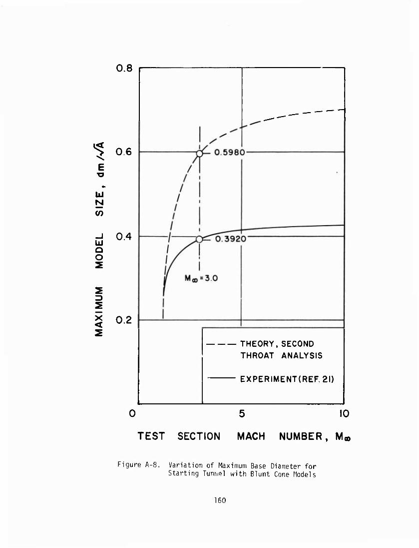
0.8
^ 0.6 E
lü N
CO
Q O 2
0.4
x < 2
0.2
THEORY,SECOND THROAT ANALYSIS
EXPERIMENT(REF.2I)
10
TEST SECTION MACH NUMBER, M«,
Figure A-8. Variation of Maximum Base Diameter for Starting Tunnel with Blunt Cone Models
160

30
I- o z ÜJ
UJ z o o
20
S 10 X <
100 200
INVISCID TEST SECTION AREA. ACIN^)
Figure A-9. Variation of Maximum Cone Length with Inviscid Test Section Size for Shock Reflection Limited Cases
161

30
5 20 Lü
IxJ CD Q Lü
X < 2
10
0 100 200
INVISCID TEST SECTION AREA,A(IN )
Figure A-10. Variation of Maximum Wedge Length with Inviscid Test Section Size for Blockage Limited Cases
162

4.0 CM
u UJ
GO
<
< UJ
<
3.0
co 2.0 tu '-•^ i-
cr LU a.
o _i Ü-
<
1.0
To' '350oR s
MOJO.O
//
400° R —s N\
///
4500R —s \ x ^w////
500oR —s \\ W///
^
5500R s
p r
200 400
STAGNATION PRESSURE, P0 (PSIA)
600
Figure A-ll. Mass Flow per Unit Test Section Area as a Function of Tunnel Stagnation Conditions
163

60
CM
h- LL
< ÜJ
<
-I < Z o
Ü UJ (0
I CO 0) o or o
UJ ÜJ or
UJ ü z UJ
CO
40
20
Mo, = 3.0
713' x 713' 8.06' DIA
P0=500 PSIA
T0 = 5000R
/ \ / 1
/ 1 / 1
4.76'x 4.76' J 5.38' DIÄ X
r 1 i i
I •
/ 8Hl <8"
•
I2"xl2"
i 100 200
INVISCID TEST SECTION AREA {\WC)
Figure A-12. Variation of Silencer Size with Test Section Size for a Silencer Intake Velocity of 100 ft/sec
164

IO I O X
IO
ü.
LU a: ID O UJ or
UJ
9
Ü
DU
i
lMo> = 3.0 | PREDICTED RANGE OF OPFRATION
|P0=6.86PS A]
T0»500oR | Re/I =1.2 xlO6
|t=60 SECS |
/!
/1 40
/ 1 1 / |
X« 5.40 -A / y • i
1 A X-2.75 -^7 \A A
20 / \ A r
A/ ^
■ i I
//\
// 8"x8" 12% 12"
100 200
INVISCID TEST SECTION AREA.A(IN^)
Figure A-13. Variation of Required Vacuum Volume with Test Section Size for a 60-second Run at a Unit Reynolds Number of 1.2 x IO6 per Foot
165

15
ro i O
K ro
Q
O a:
o >
UJ
< Q: o
<
10
/ i
/
1
Moo = 30
IF. = eoopsiA T0 =500OR
/
/ po =
t = 180 SECS
PST= 2200 PSIA
Ps « 2.5 P0
500PSIA /
556PSIA^ f , / /
Y 1 ; ' Po = 400PSIA y
_8250_fT_3_A S-J-- / ^SSIPSIA^
/
//
/
|P0 = 300PSIA
///
/ /
P0 = 200 PSIA
/^/ J>0 * 100 PSIA"
^—5" iS" I2"XI2M
100 200
INVISCID TEST SECTION AREA.ACIN^)
Figure A-14. Variation of Air Storage Volume Requirements with Test Section Size and Operating Pressure
166

10 8
z ÜJ
ÜJ a o
Q ÜJ CO < GO
Ql LÜ GO
cn Q -J O z Lü a:
10
Ma)5 3.0
-
T0 =500oR
V =8250 FT3
Pst = 2200PSIA Ps=25Po
i
-/
< <
< en Q_
< en Q.
< cn a.
cn a. cn
cn a. ro
i ••— OD CVJ'
(0 5 00 rO n
CVJ
in H II H
ii
o o
Q. o 0. •
Q.1 Q.
Q. _ 2
_ O OJ 12 'oo "bo "^
i
M X X X X
^ - . -
'oo O "CVJ in 2
_J L_™~__J 1
200 400 INVISCID TEST SECTION AREA(INZ)
Figure A-15. Maximum Model Reynolds Number Attainable as a Function of Inviscid Test Area
167

O O
LJ Ü-
cn 10 LJ GD
CO Q _l O
>- Lü
H
3
< LÜ cr
UJ UJ a:
8
10'-
10 -
Moo = 3.0
570
ATMOSPHERIC EXHAUST
CONDITIONAL OPERATION
PSIA
DESIGN POINT
ATMOSPHERIC EXHAUST
VACUUM EXHAUST
CONDITIONAL OPERATION
B
VACUUM EXHAUST
5 PSIA
300 400 500 600
TUNNEL STAGNATION TEMPERATURE (0R)
Figure A-16. Predicted Tunnel Performance Envelope
168
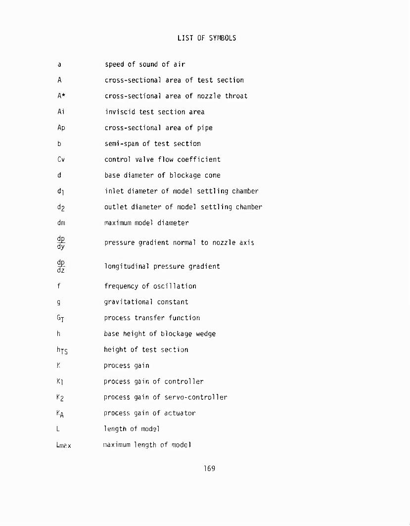
LIST OF SYMBOLS
a speed of sound of air
A cross-sectional area of test section
A* cross-sectional area of nozzle throat
Ai inviscid test section area
Ap cross-sectional area of pipe
b semi-span of test section
Cv control valve flow coefficient
d base diameter of blockage cone
d] inlet diameter of model settling chamber
02 outlet diameter of model settling chamber
dm maximum model diameter
d£ dy
pressure gradient normal to nozzle axis
-j^- longitudinal pressure gradient
f frequency of oscillation
g gravitational constant
Gj process transfer function
h base height of blockage wedge
hjj height of test section
K process gain
K] process gain of controller
K2 process gain of servo-controller
K/\ process gain of actuator
L length of model
Lmax maximum length of model
169

LIST OF SYMBOLS (CONT'D)
Ln length of nozzle measured from throat
Lp length of a section of pipe
if) mass flow rate
m quasi-steady nozzle mass flow rate
M local Mach number in flow field
Mrms root-mean-square Mach number based upon local Mach number measurements
Mw Mach number at tunnel wall
Mx local Mach number at distance x
pc static pressure in test section
Pd stat c pressure in diffuser
pe static pressure in exhaust duct or vacuum sphere
p0 quasi-steady settling chamber pressure
P local static pressure
P] supply line static pressure at inlet to isolation valve
Pz supply line static pressure at inlet to isolation valve
Pcond static pressure at onset of air condensation
P0 stagnation pressure or settling chamber pressure
PQ measured pitot pressure
Ps supply line static pressure at inlet to control valves
P5J pressure in storage tanks
Pw measured nozzle or diffuser wall static pressure
r/R normalized radial distance in model settling chamber
r/As normalized radial distance from nozzle axis to impact probe
ReLn Reynolds number based on nozzle length
170
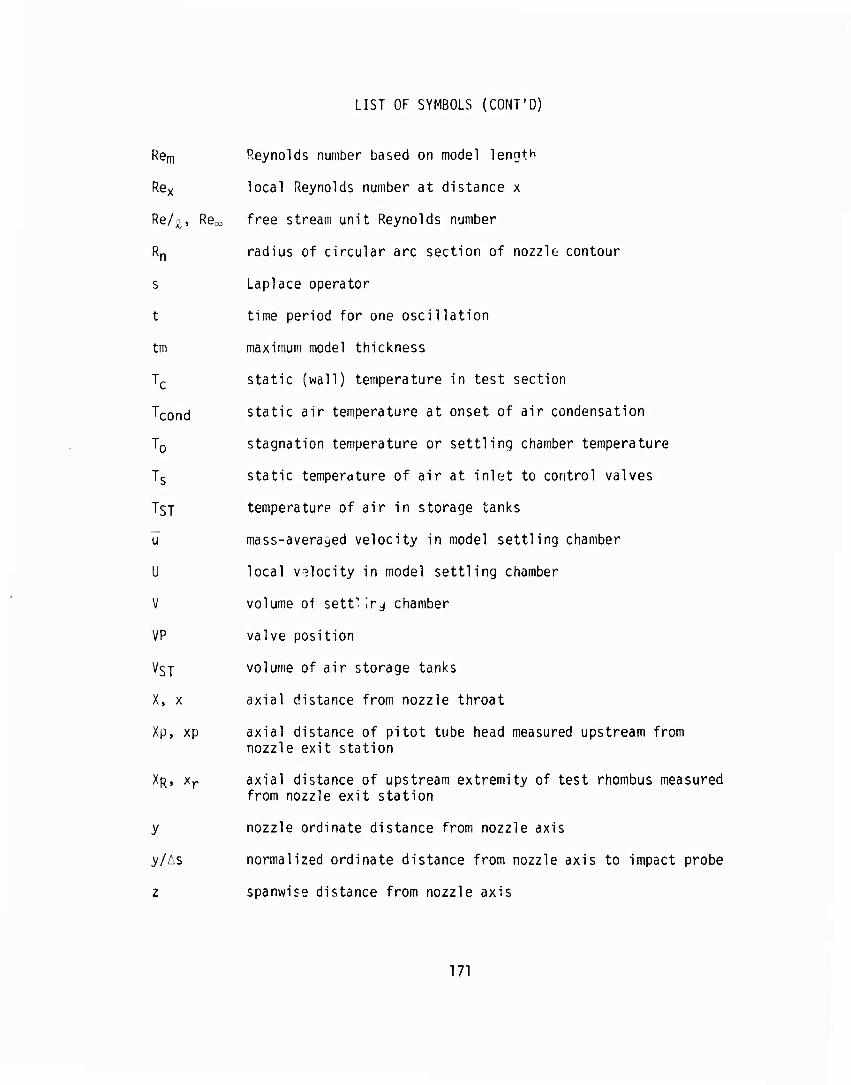
LIST OF SYMBOLS (CONT'D)
Rem Reynolds number based on model length
Rex local Reynolds number at distance x
Re/£, Reoo 'free stream unit Reynolds number
Rn radius of circular arc section of nozzle contour
s Laplace operator
t time period for one oscillation
tm maximum model thickness
Tc static (wall) temperature in test section
Tcond static air temperature at onset of air condensation
T0 stagnation temperature or settling chamber temperature
Ts static temperdture of air at inlet to control valves
TST temperature of air in storage tanks
u mass-averaged velocity in model settling chamber
U local velocity in model settling chamber
V volume of sett1 irj chamber
VP valve position
VSJ volume of air storage tanks
X, x axial distance from nozzle throat
Xp, xp axial distance of pi tot tube head measured upstream from nozzle exit station
XR, xr axial distance of upstream extremity of test rhombus measured from nozzle exit station
y nozzle ordinate distance from nozzle axis
y/As normalized ordinate distance from nozzle axis to impact probe
z spanwise distance from nozzle axis
171

LIST OF SYMBOLS (CONT'D)
AA^ total blockage area
Ap pressure differential or pressure drop
As pi tot probe spacing on Mach number survey rake
Aj temperature differential due to throttling and expansion = l^j - T0
AV change in fluid velocity in pipe
A angle of attack
c, flow angularity
6* local displacement thickness of boundary layer at distance x
f displacement thickness at nozzle exit
Y ratio of specific heats for air
> tunnel pressure ratio
ij Mach angle
$ roll angle of survey rake measured clockwise from horizontal plane looking upstream
p density of air
half-angle of wedge or cone model
T process time constant
r] process time constant of controller
'2 procesr time constant of servo-controller
[ß process time constant of actuator
0 included angle of flow angularity cone or wedge
o«. shock angle
172
U.S.Grn/ernmem Printing Offi.c: 1975 6b7-020/483