Embed Size (px)
Citation preview

AFdSR.TR. 9 1 0~ 29
AD-A244 131
IjI
o.4
91-19201
SECURITY CLASSIFICATTON OP THIS PAGEI Form Approved
REPORT DOCUMENTATION PAGE OMBNo. 0704-0188
la. REPORT SECURITY CLASSIPICATION lb. RESTRICTIVE MARKINGS
Unclassified __,
2a. SECURITY CLASSIFICATION AUTHORITY 3. DISTRIBUTIONIAVALABILITY OF REPORT
2b. DECLASSIFICATION /DOWNGRADING SCHEDULE Approvej for public release,_ distributionuullliaited
4. PERFORMING ORGANIZATION REPORT NUMBER(S) S. MONITORING ORGANIZATION REPORT NUMBER(1S)
6a. NAME OF PERFORMING ORGANIZATION 6b. OFFICE SYMBOL 7a. NAME OF MONITORING ORGANIZATION
University of Colorado (If applicable) Air Force Office of Scientific Researchat Boulder I CEAE Dept. AFOSR/NA
6c. ADDRESS (City, State, and ZIPCode) 7b. ADDRESS (City, State, and ZIP Code)
Dept. Civil, Env., and Arch. Engineering Building 410Boulder, Colorado 80309-0428 Bolling Air Force Base, DC 20332-6448
Ba. NAME OF FUNDING/SPONSORING Bb. OFFICE SYMBOL 9. PROCUREMENT INSTRUMENT IDENTIFICATION NUMBER
ORGANIZATION ZS-AF I (If applicable)
Office of Scientific Research I AFOSR/NA AFOSR-89-02898c. ADDRESS (City, State, and ZIP Code) 10. SOURCE OF FUNDING NUMBERS
BalngAr. c BPROGRAM PROJECT TASK jWORK UNITBozlng Air Force Base IELEMENT NO. NO, NO. ACCESSION NO.
Washington, D.C. 20332-6448 61102 F 2302 C2
11. TITLE (Include Security Classification)
Brittle Ductile Failure Mechanics of Mortar and Concrete
12. PERSONAL AUTHOR(S)Sture, Stein, Willam Kaspar J., and Saouma, V.
13a. TYPE OF REPORT 13b. 114. DATE OF REPORT (Year, Month, Day) 115 PAGE COUNTFinal FROM 89/4/15 9TLL30 1991, September 30 I 135
16. SUPPLEMENTARY NOTATION
17. COSATI CODES 18. SUBJECT TERMS (Continue on reverse if necessary and identify by block number)FIELD GROUP SUB-GROUP cementitious composites, fracture, slip, plasticity,
integration, work-softening, stability, tension-shear and
compression-shear experiments, polygonization.19. ABSTRACT (Continue on reverse if necessary and identify by block number)The final technical report summarizes analysis and results comprising both theory and
experiments related to modeling of interfaces between cement matrix and aggregate. The
model simulates accurately behavior under complex two and three-dimensional states ofstress and deformation, where tension-shear and compression-shear conditions occur. The
constitutive theory describes fracture and slip of the interface, and adhesion, debonding,and mobilized friction mechanisms are modeled. Fracture energy release is used to controlsoftening. Analytical predictions of experiments compare well, and the model has been
implemented in nonlinear finite element analysis codes.
Two theses (Ph.D., Thomas Stankowski; MS, Philippe Menetrey) and eight scientific papers
have been prepared under the auspices of the project.
20. DISTRIBUTION/AVAILABILITY OF ABSTRACT 21. ABSTRACT SECURITY CLASSIFICATION
EN UNCLASSIFIED/UNLIMITED 0] SAME AS RPT. 0 DTIC USERS 1Jnclaqq[f1Pd
22a. NAME OF RESPONSIBLE INDIVIDUAL 22b. TELEPHONE (Include Area Code) 22c. OFFICE SYMBOLDr. Spencer T. Wu (202) 767-6962 I AFOSR/NA
DO Form 1473, JUN 86 Previous editions are obsolete. SECURITY CLASSIFICATION OF THIS PAGE
I CU NL A SV F! r D
ISPORT DOCUMENTATION PAGE -3, A
30 Sept., 1991 Final, April 1989 - Sept. 1991
Brittle ductil failure mechanics of mortar and con ete AFOSR-89-0289 G
Stein Sture, Kaspa Willam, and
Victor Saouma
Department of Civil, vironmental, and Arc tecturalEngineeringUniversity of Colorado a BoulderColorado 80309-0428I/Air Force Office of Scientif Research AFOSR/NABuilding 410Bolling Air Force BaseWashington, DC 20332-6448
The ina reortsummarizes an lysis and re Its comprising both theory and
experiments related to modeli of interface between cement matrix and aggregate.
The model simulates accuratel behavior under complex two- and three-dimensional
Istates of stress and deformat on, where tensi -shear and compression-shear condi-
tions occur. The constituti e theory describe fracture and slip of the interface,
and adhesion, debonding, and mobilized friction mechanisms are modeled. Fracture
energy release is used to co trol softening. An lytical predictions of experiments
comape well, and the model as been implemented nonlinear finite element analy-
sis codes.
* Two theses (Ph.D.; Thomas S ankowski, MS; Philipp Menetrey) and eight scientific
papers have been prepared der the auspices of the project.
14 UBJECT TERMS 15. 4 V.1id ER
*cementitious composites; racture; slip; plasticity; inte- 135
gration; work-softening; stability; tension-shear and compres- '6 " cE
sion-shear experiments; olygonization. ._....17 A,, CL.iSiFCA ,C 13. SEURTY C'AS S' C r RITY CLASSi: CAT-ON 0. 1
OF RPEVOT TOTIS 24GE ,I F 2F3STRACT
Unclassified Unclassified t Unclassified UL
TABLE OF CONTENTS
Page
1. Executive Summary .... .................. 2
2. List of Publications in the Project ... ....... 3
PART 1 FRACTURE AND SLIP OF INTERFACESIN CEMENTITIOUS COMPOSITES, MODELCHARACTERISTICS ...... ............... . . 1
Abstract. . . . ......................... 2
Contents ............ ........................ 3
1. Introduction ................. .. . ... .. 4
2. Concepts of Fracturing and Slip. . . . . . . . .. 5
3. Fracture/Slip Criterion ..... .............. 7
4. Postfailure Behavior ....... ............... 8
5. Uniqueness of Response - Brittle Behavior . . . .12
6. Calibration . . . . . . . . . . . .......... 17
7. Application . ..................... 17
8. Appendix I: References ..... ............ 19
9. Appendix II: Notation . . . . . . ....... 21
10. Appendix III: The Construction of VoronoiPolyhedra in Three Dimensions . .. 23
PART 2 MODEL IMPLEMENTATION ............. 1
1. Introduction . . . . . . . . . . . . . . . . . . . 3
* 2. Incremental Relations ............... 3
2.1 Implicit Integration. . . . . . . ...... 3
2.2 Newton Iteration. . . . . . . . . . . . . . . 5
2.3 Interpolation/Iteration Scheme . . . . . . . . 6
* 2.4 Iterative Procedure for Mixed Control .... 8
0. m m m m

3. Finite Element Modeling with Interfaces . . . . .. 8
3.1 Basic Equations ............... 8
3.2 Iterative Scheme - Numerical Performance . . .10
4. Numerical Results ....... ................ . 12
5. Summary and Conclusions ...... .............. .13
6. Appendix I: Algorithmic Tangent Stiffness . . . .15
7. Appendix II: Extension of the Model to ThreeDimensions ..... ............. .17
8. Appendix III: References ..... ............. .18
9. Appendix IV: Notation ...... ............... .19
PART 3 INTERFACE EXPERIMENTS. . . . ........... 1
1. Introduction ..................... 1
2. Apparatus . . . ...................... 1
3. Experiments ............. . . . . . . . 2
4. Experimental Data ........ ................. 3
5. List of Figures ......... .................. 5
Acoosslo Fr
f it tjDistribution/
rAv~iliblity Codes(D s Sposi a ld s
IA
1. EXECUTIVE SUMMARY
This is the final technical report in the AFOSR supportedproject entitled, Brittle Ductile Failure Mechanics ofMortar and Concrete. The report summarizes theory, analy-sis, and experimental results obtained in model studies oncement matrix (mortar) and aggregate (stone).
This report describes the theory, implementation, andpredictive capabilities of a new and relatively straight-forward constitutive theory for interfaces, that describesfracture, slip and post-peak and residual behavior formortar-aggregate composites (concrete). Adhesion, debondingand mobilized friction are accounted for in the character-ization of interface behavior, and the debonding is control-led through a work-softening rule, that incorporates tensilecrack opening as well as tangential slip. The materialparameters have clear physical meaning and can be calibratedfrom conventional and special interface experiments. Thepredictive performance of the model is tested on both largeand small composite structures, and the results compare wellto those obtained in laboratory experiments.
The last part of the report contains data from mortar-
aggregate interface experiments, where small specimens weresubjected to combinations of tensile and shear or comp-ression and shear loading. Experimental technique andapparatus are also described.
The report comprises three parts, which are organized asfollows: Part 1; Modeling of fracture and slip of interfacesin cementitious composites (model characteristics), Part 2;Model implementation, and Part 3; Interface experiments.
Several publications have been prepared in the project, andthe bibliography is attached on the next page. Additionaljournal and conference papers will also be prepared based onthe contents of this report.
LIST OF PUBLICATIONS PREPARED IN THE PROJECT
"Simulation of Failure Processes in Cementitious ParticleComposites," by T. Stankowski, S. Sture, K. Runesson, and K.Willam, in Proc. ASCE Engineering Mechanics Division,Specialty Conference, May 19-22, 1991, Columbus, Ohio,pp. 1102-1107.
"Simulation of Failure Processes in Cementitious Composites- Concrete," by T. Stankowski, S. Sture, K.J. Willam, and K.Runesson, Proc. Int. Conf. Fracture Processes in BrittleDisordered Materials, June 19-21, 1991, Noordwijk, TheNetherlands.
"Progressive Failure Analysis of Cementitious Composites,"by T. Stankowski, S. Sture, and K. Runesson, in Proc. Int.Conf. Constitutive Laws for Engineering Materials, RecentAdvances and Industrial and Infrastructure Applications,Univ. of Arizona, Tucson, Jan. 1991, pp. 627-632.
"Numerical Simulation of Failure in Particle Composites," byT. Stankowski, Proc. World Conf. Computational Mechanics,Stuttgart, August, 1990.
"Theory and Basic Concepts for Modelling Concrete Behavior,"K.J. Willam, T. Stankowski, and S. Sture,Comite Euro-International du Beton (CEB)Bulletin 194, Modelling of Structural Reinforced andPresetressed Concrete in Computer Programs,May, 1990, pp. 15-43.
"Numerical Simulation of Progressive Failure in Particle
Composites", T. Stankowski, Ph.D. Thesis, Department ofCivil, Env., and Arch. Engineering, University of Coloradoat Boulder, 1990, 118 pp.
A Three-Dimensional Model Based on the Finite Element Methodand Plasticity Theory to Analyze Plain Concrete Structures,"P. Menetrey, MS Thesis, Department of Civil, Env., and Arch.Engineering, University of Colorado at Boulder, August,1991, 128 pp.
"Simulation Issues of Distributed and Localized FailureComputations," by K.J. Willam, T. Stankowski, K. Runesson,and S. Sture, Proc. Cracking and Damage- Strain Localizationand Size Effects, Eds. J. Mazars and Z.P. Bazant, ElsevierAppl. Sci., London, 1989, pp. 363-378.
"Combined Compression-Shear Experiments on MOrtar-AggregateInterfaces," by T. Stankowski, S. Sture, and K. Runesson,Proc. ASCE, Mateerials Eng. Div. Congress, Denver, Colorado,August, 1990, Vol. I, pp. 350-359.
p
FRACTURE AND SLIP OF INTERFACES
IN CEMENTITIOUS COMPOSITES
Part I: Model Characteristics
by
T. Stankowski1 , K. Runesson 2, S. Sture3
1Res. Assoc., Dept. of Civil, Environmental, and Architectural Engrg., University of Colorado,Boulder, CO 80309.
2 Visit.Prof., Dept. of Civil, Environmental, and Architectural Engrg., University of Colorado,Boulder, CO 80309.
3 Prof., Dept. of Civil, Environmental, and Architectural Engrg., University of Colorado, Boulder,CO 80309.
Abstract:
A new and relatively simple constitutive theory that describes fracture and slip ofan interface in cementitious composites such as concrete is presented. Adhesion,debonding and mobilized friction mechanisms are considered in the characterization
D of the interface behavior. The debonding mechanism in a state of combined normaland shear stress, i.e. the degradation of tensile and shear strengths, is monitoredvia a work-softening rule which entails tensile crack opening as well as tangentialslip. As a result, a fracture energy release based plasticity model is obtained. Thematerial parameters are physically transparent and are conveniently calibrated fromcharacteristic response functions that can be observed experimentally in pure tensionand in pure shear. Analytical predictions are compared with experimental resultsfor the case when constant normal traction is applied while the slip displacement ismonitored.
2

Contents
1 INTRODUCTION 4
2 CONCEPTS OF FRACTURING AND SLIP 5
3 FRACTURE/SLIP CRITERION 7
4 POSTFAILURE BEHAVIOR 8
5 UNIQUENESS OF RESPONSE - BRITTLE BEHAVIOR 12
6 CALIBRATION 17
7 APPLICATION 17
8 APPENDIX I: REFERENCES 19
9 APPENDIX II: NOTATION 21
10 APPENDIX III: THE CONSTRUCTION OF VORONOI2POLYHEDRA IN THREE DIMENSIONS 23
3
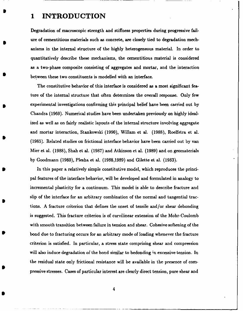
1 INTRODUCTION
Degradation of macroscopic strength and stiffness properties during progressive fail-
ure of cementitious materials such as concrete, are closely tied to degradation mech-
anisms in the internal structure of the highly heterogeneous material. In order to
quantitatively describe these mechanisms, the cementitious material is considered
as a two-phase composite consisting of aggregates and mortar, and the interaction
between these two constituents is modelled with an interface.
The constitutive behavior of this interface is considered as a most significant fea-
ture of the internal structure that often determines the overall response. Only few
experimental investigations confirming this principal belief have been carried out by
Chandra (1969). Numerical studies have been undertaken previously on highly ideal-
ized as well as on fairly realistic layouts of the internal structure involving aggregate
and mortar interaction, Stankowski (1990), Willam et al. (1988), Roelfstra et al.
(1985). Related studies on frictional interface behavior have been carried out by van
Mier et al. (1988), Shah et al. (1987) and Atkinson et al. (1989) and on geomaterials
by Goodmann (1980), Plesha et al. (1988,1989) and Gilette et al. (1983).
In this paper a relatively simple constitutive model, which reproduces the princi-
pal features of the interface behavior, will be developed and formulated in analogy to
incremental plasticity for a continuum. This model is able to describe fracture and
slip of the interface for an arbitrary combination of the normal and tangential trac-
tions. A fracture criterion that defines the onset of tensile and/or shear debonding
is suggested. This fracture criterion is of curvilinear extension of the Mohr-Coulomb
with smooth transition between failure in tension and shear. Cohesive softening of the
bond due to fracturing occurs for an arbitrary mode of loading whenever the fracture
criterion is satisfied. In particular, a stress state comprising shear and compression
will also induce degradation of the bond similar to bedonding ;n excessive tension. In
the residual state only frictional resistance will be available in the presence of com-
pressive stresses. Cases of particular interest are clearly direct tension, pure shear and
4
SM
direct compression. The constitutive relations are regularized by the introduction of
a recoverable adhesion component in the tangential as well as the normal directions.
A non-associated slip rule is used in order to account for dilatancy effect in a realistic
* manner.
In Part II of this paper we discuss the numerical technique that is used to integrate
the constitutive relations in a step-by-step fashion. A robust incremental solution
technique is essential for the successful application of the constitutive model to solve
boundary value problems.
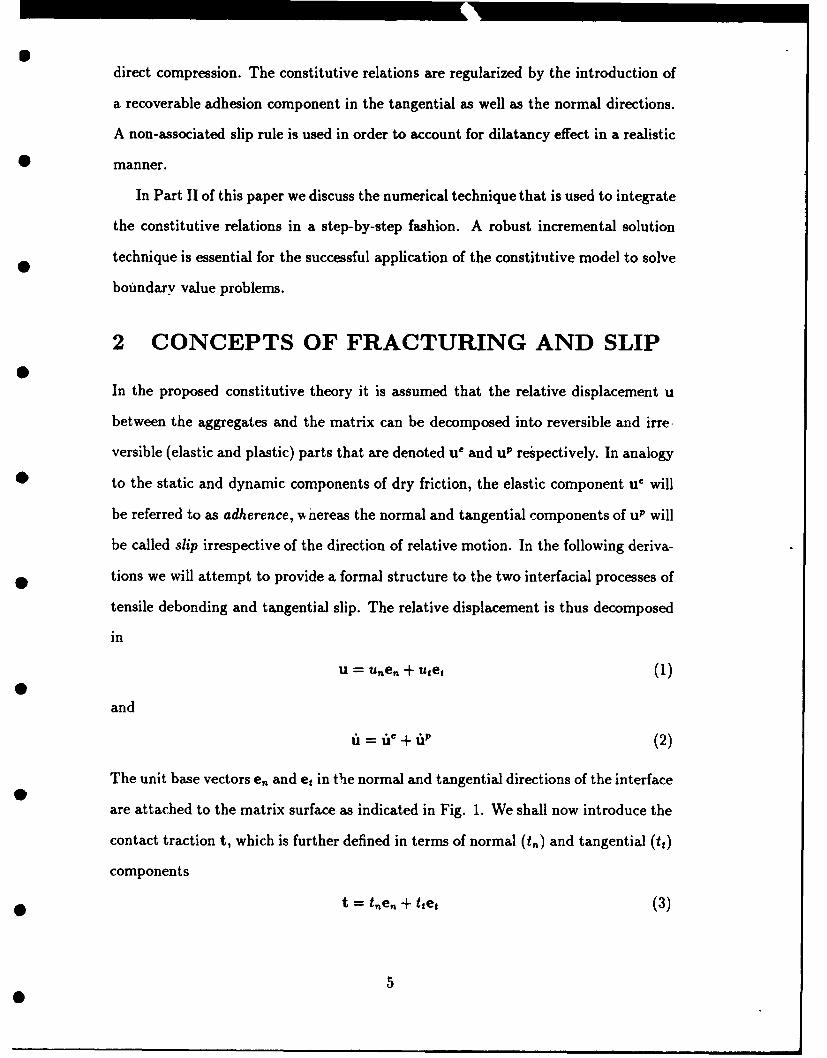
2 CONCEPTS OF FRACTURING AND SLIP
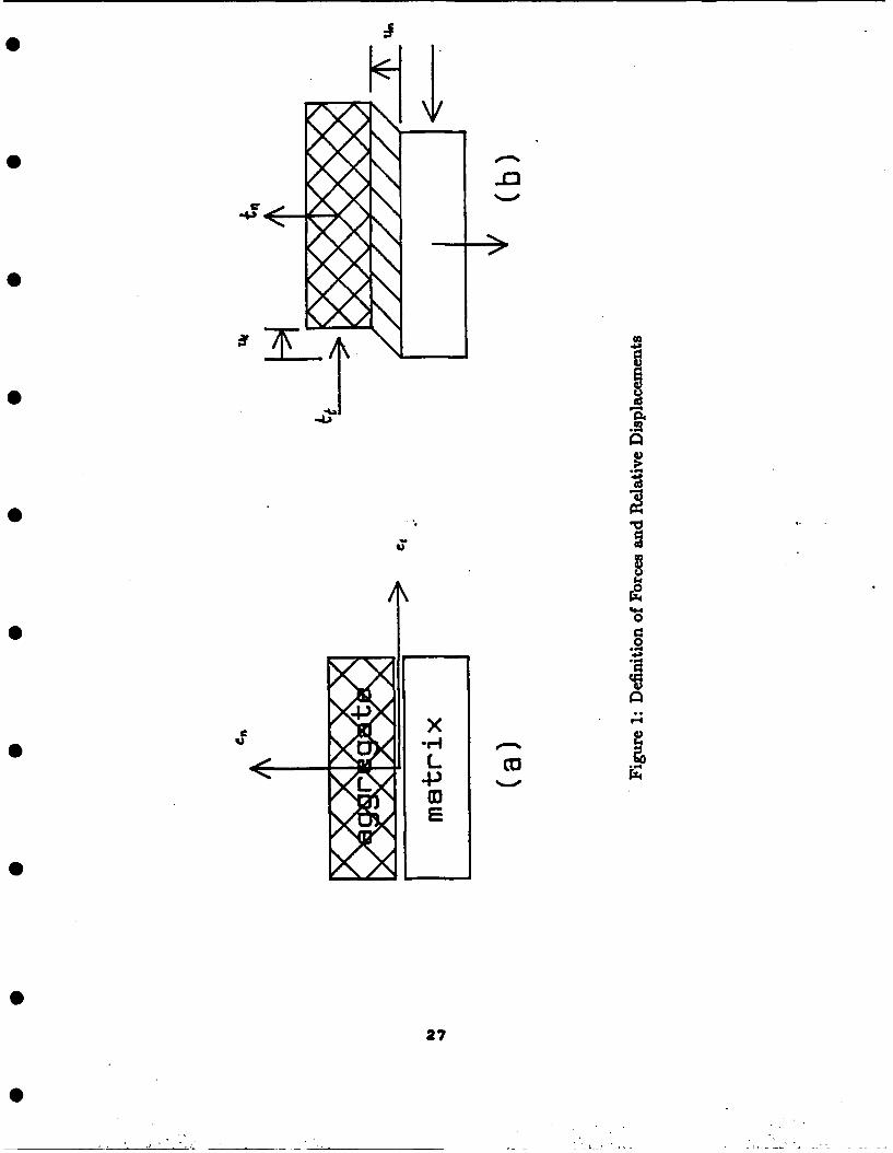
In the proposed constitutive theory it is assumed that the relative displacement u
between the aggregates and the matrix can be decomposed into reversible and irre
versible (elastic and plastic) parts that are denoted Ue and uP respectively. In analogy
* to the static and dynamic components of dry friction, the elastic component uC will
be referred to as adherence, v nereas the normal and tangential components of uP will
be called slip irrespective of the direction of relative motion. In the following deriva-
tions we will attempt to provide a formal structure to the two interfacial processes of
tensile debonding and tangential slip. The relative displacement is thus decomposed
in
u = unen + utet (1)
and
, = f + 6 (2)
The unit base vectors en and et in the normal and tangential directions of the interface0
are attached to the matrix surface as indicated in Fig. 1. We shall now introduce the
contact traction t, which is further defined in terms of normal (4a) and tangential (it)
components
t = te, + ttet (3)
50
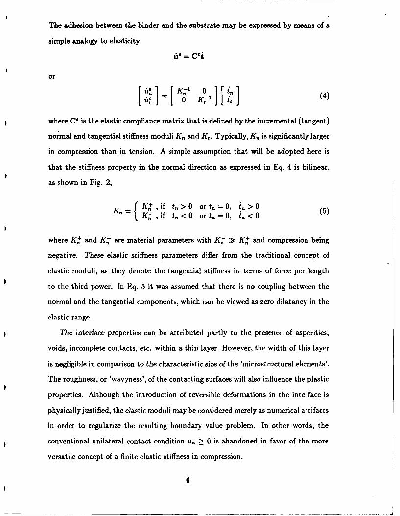
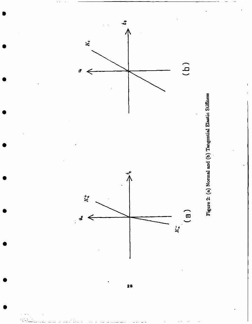
The adhesion between the binder and the substrate may be expressed by means of a
simple analogy to elasticity
or
K;" 0(4)
where C1 is the elastic compliance matrix that is defined by the incremental (tangent)
normal and tangential stiffness moduli K, and Kt. Typically, K is significantly larger
in compression than in tension. A simple assumption that will be adopted here is
that the stiffness property in the normal direction as expressed in Eq. 4 is bilinear,
as shown in Fig. 2,
Kn K+,if t,,>O0 or4.=O0, .>O0K K= K ,if t,,< 0 or t,,=0, i< 0(5
where K + and K; are material parameters with K; > K + and compression being
negative. These elastic stiffness parameters differ from the traditional concept of
elastic moduli, as they denote the tangential stiffness in terms of force per length
to the third power. In Eq. 5 it was assumed that there is no coupling between the
normal and the tangential components, which can be viewed as zero dilatancy in the
elastic range.
The interface properties can be attributed partly to the presence of asperities,
voids, incomplete contacts, etc. within a thin layer. However, the width of this layer
is negligible in comparison to the characteristic size of the 'microstructural elements'.
The roughness, or 'wavyness', of the contacting surfaces will also influence the plastic
properties. Although the introduction of reversible deformations in the interface is
physically justified, the elastic moduli may be considered merely as numerical artifacts
in order to regularize the resulting boundary value problem. In other words, the
conventional unilateral contact condition u,, > 0 is abandoned in favor of the more
versatile concept of a finite elastic stiffness in compression.
6

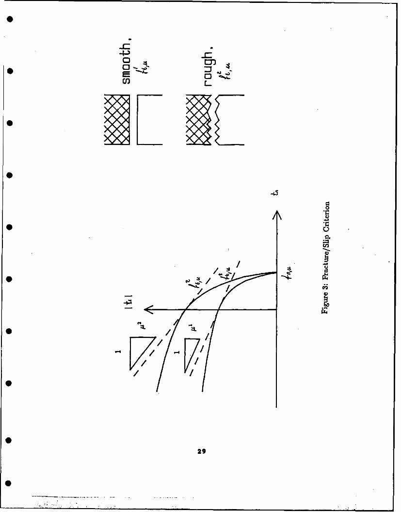
3 FRACTURE/SLIP CRITERION
In pure tension the strength is characterized by the tensile peak (or ultimate) strength
f,.,. In combined normal and shear loading, however, the strength comprises the ad-
hesion f t,. between the different materials and the mobilized friction due to the pres-
ence of a normal traction t, 5 0. This friction is considered to be a consequence of the
mineral to mineral surface friction and geometric roughness between the contacting
surfaces. The adhesion, which is the equivalent of the cohesion within a continuous
material, is sometimes called the slip limit.
Clearly, the two mechanisms of tensile debonding in the normal direction e, and
slip in the tangential direction et are physically connected in the sense that slip may
be be viewed as a consequence of a crack that develops along the interface, whereby
the bond strength is degrades further. In the event that one or both mechanisms are
activated it seems appropriate to introduce the notation Fracture Criterion for the
surface in (tn, tt)-space that represents the onset of inelastic displacements. A simple
Fracture Criterion can be expressed as
F =1 ti (f'tu)"(f, - t,) = 0 (6)
fn,u
where f,, denotes the current value of the normal strength. The current value of the
shear strength is denoted by ft (and is used later). The peak, or initial, strength
values are denoted fn,. and ft,. respectively, and it follows that
tn < fn , 0<5A f< ,u (7)
Itt I< fA (8)
The shape of the slip surface is such that the normal is horizontal at the tensile apex
(t,, tt) = (f,, 0). Furthermore, a constant exponent a > 1, that determines the shape
of the surface, is defined in terms of the coefficient of friction p when tn = 0 according
to the expression
a fn,u 97ft,
7
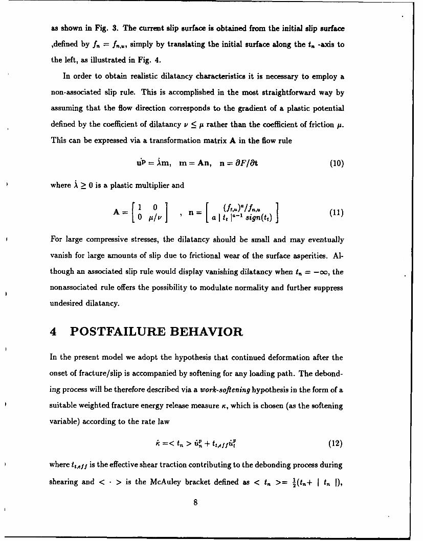
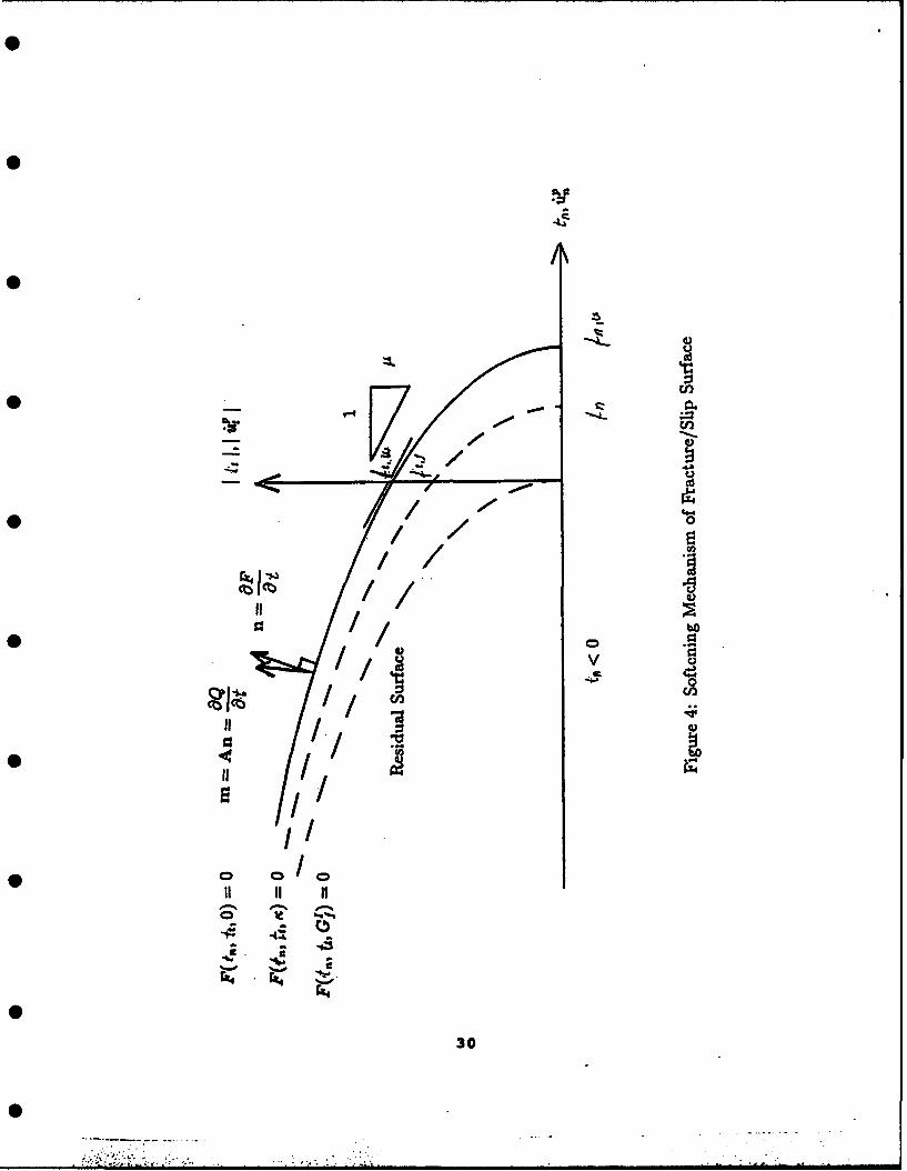
as shown in Fig. 3. The current slip surface is obtained from the initial slip surface
,defined by f, = , simply by translating the initial surface along the t. -axis to
the left, as illustrated in Fig. 4.
In order to obtain realistic dilatancy characteristics it is necessary to employ a
non-associated slip rule. This is accomplished in the most straightforward way by
assuming that the flow direction corresponds to the gradient of a plastic potential
defined by the coefficient of dilatancy v < p rather than the coefficient of friction p.
This can be expressed via a transformation matrix A in the flow rule
uP = Am, m = An, n = OFot (10)
where A > 0 is a plastic multiplier and
A = 0 [ , n = a r (f'*a-' gU ,
For large compressive stresses, the dilatancy should be small and may eventually
vanish for large amounts of slip due to frictional wear of the surface asperities. Al-
though an associated slip rule would display vanishing dilatancy when t,, = -oo, the
nonassociated rule offers the possibility to modulate normality and further suppress
undesired dilatancy.
4 POSTFAILURE BEHAVIOR
In the present model we adopt the hypothesis that continued deformation after the
onset of fracture/slip is accompanied by softening for any loading path. The debond-
ing process will be therefore described via a work-softening hypothesis in the form of a
suitable weighted fracture energy release measure K, which is chosen (as the softening
variable) according to the rate law
iC=< tn > i pn + t,,ff'Ot (12)
where t t,eff is the effective shear traction contributing to the debonding process during
shearing and < > is the McAuley bracket defined as < t,, >= (,+ I t )
8
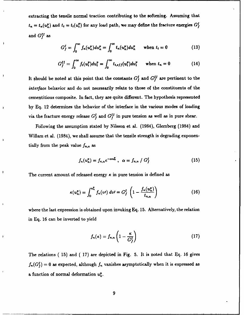
extracting the tensile normal traction contributing to the softening. Assuming that
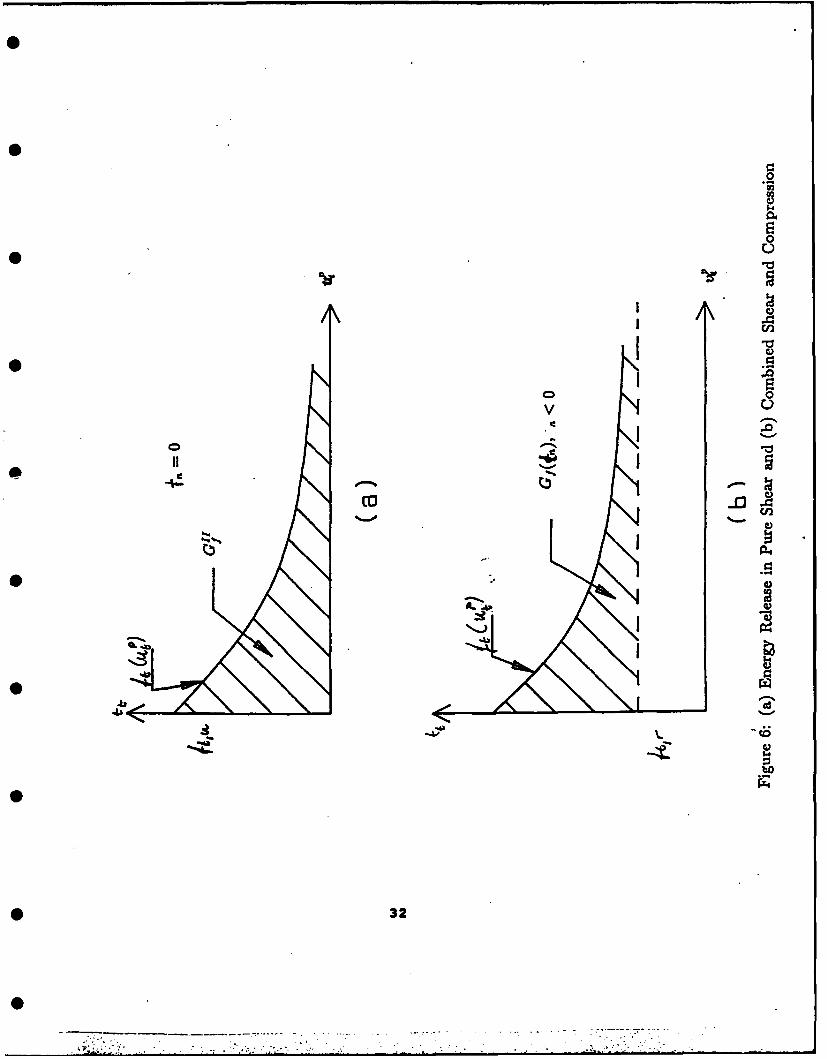
t" = it,(uP) and tt = tt(uP) for any load path, we may define the fracture energies GI
and GII as
G= - f (u )duP = tn(P)duP when tt = 0 (13)
G I 00 ft(t4)duP = j0 t,fei(uP)duP when t, = 0 (14)
It should be noted at this point that the constants GI and GII are pertinent to the
interface behavior and do not necessarily relate to those of the constituents of the
cementitious composite. In fact, they are quite different. The hypothesis represented
by Eq. 12 determines the behavior of the interface in the various modes of loading
via the fracture energy release GI and G11 in pure tension as well as in pure shear.
Following the assumption stated by Nilsson et al. (1984), Glemberg (1984) and
Willam et al. (1984), we shall assume that the tensile strength is degrading exponen-
tially from the peak value fn,u as
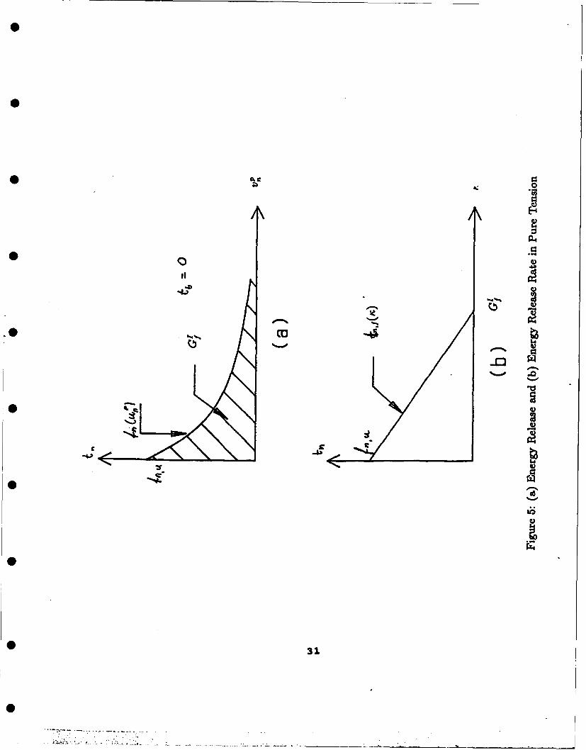
f,(u") = fn,ue - ' , a = fn,,, / GI (15)
The current amount of released energy x in pure tension is defined as
UPf.(up.) 16
Pc(u") = j fn(vi) dvi = G1 1 - (16)
where the last expression is obtained upon invoking Eq. 15. Alternatively, the relation
in Eq. 16 can be inverted to yield
fnI)= f,u (1 (17)
The relations (15) and (17) are depicted in Fig. 5. It is noted that Eq. 16 gives
f,(GI) = 0 as expected, although f,, vanishes asymptotically when it is expressed as
a function of normal deformation u .
9

Defining the effective shear traction as
tt,,.f = k(tt - ft,,) (18)
where k is the ratio of the fracture energy release in tension and shear, typically in
the range k - 0.01 - 0.1
f f G1ll (19)
and ft,, is the residual shear strength that remains after maximum degradation has
occured
= , A {0 (20)ft,.= f, (-t./.,u ,t. 0
we now can integrate Eq. 12 in pure shear, where t,, = 0 and tt = ft(ut)
Pe (oo) = k0 ft(uP) duP = k G = G' (21)
where Eqs. 14 and 19 were used. In other words, when the interface has fractured
completely in pure tension, then the shear resistance is also exhausted corresponding
to the fact that the amount Gil of (shear) energy has dissipated and vice versa.
From these assumptions it is apparent that the characteristics of the relation between
f,, and uP will strongly determine the behavior in combined fracture and slip, since
f,(uP) is taken as the universal relationship to describe the material response.
By invoking the yield criterion in order to express ft in terms of f" when t, = 0
and by using Eq. 17, it is possible to integrate Eq. 12. This leads to a simple explicit
expression of the relation ft(4):
A,- ft, ( I Z- - - (22)
where it is the finite value of ui
a Glt f (23)
a1- ft ,
10
that is obtained when r = G1'. From Eq. 22 it is concluded that this value corre-
sponds to the vanishing of the shear strength ft, which means that ut - fit when
ft = 0 since ut = 0 at this stage. By augmenting the relation (22) with the elastic
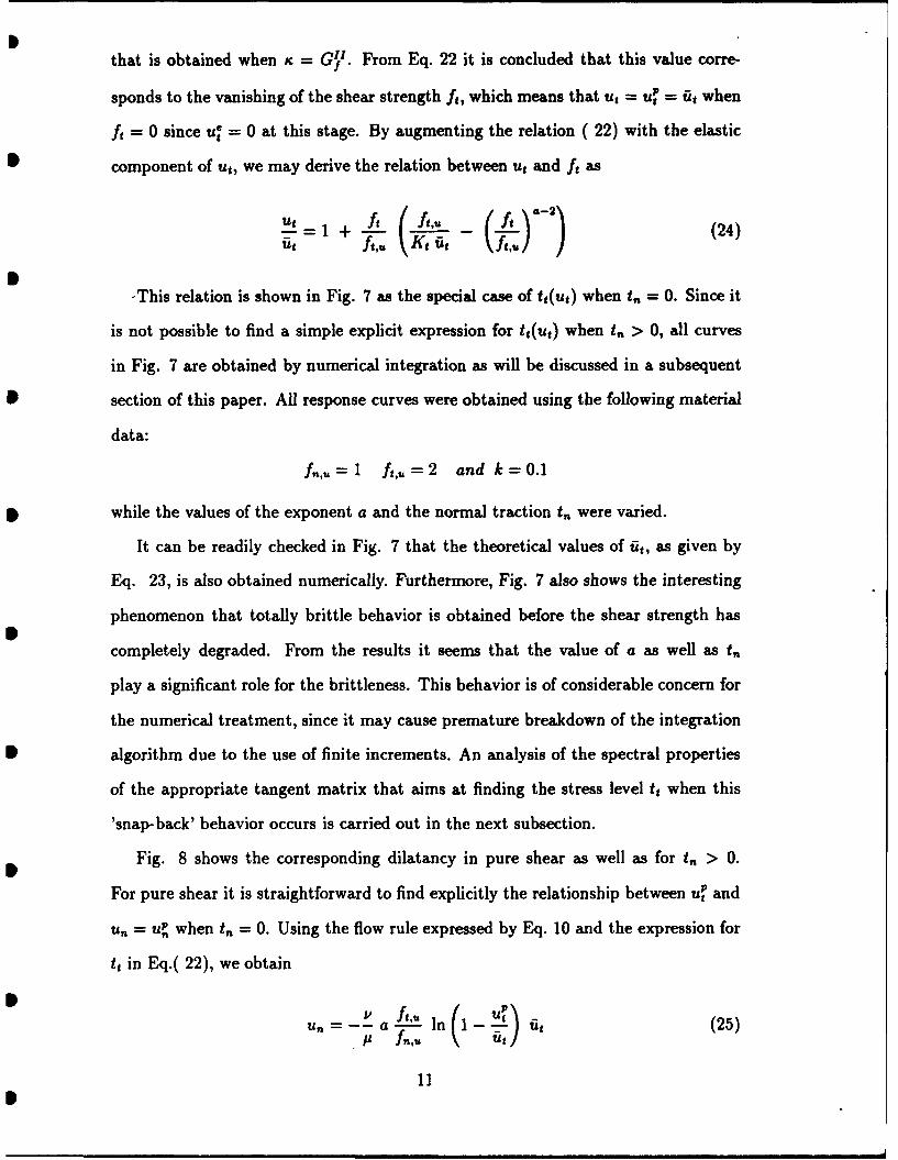
component of ut, we may derive the relation between ut and ft as
Utft((fUt +ftu Kt it ft ) 24
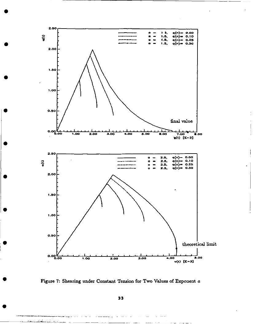
-This relation is shown in Fig. 7 as the special case of tt(ut) when t, = 0. Since it
is not possible to find a simple explicit expression for tt(ut) when t, > 0, all curves
in Fig. 7 are obtained by numerical integration as will be discussed in a subsequent
section of this paper. All response curves were obtained using the following material
data:
f.,U=l ft,,= 2 and k=0.1
while the values of the exponent a and the normal traction t4 were varied.
It can be readily checked in Fig. 7 that the theoretical values of iit, as given by
Eq. 23, is also obtained numerically. Furthermore, Fig. 7 also shows the interesting
phenomenon that totally brittle behavior is obtained before the shear strength has
completely degraded. From the results it seems that the value of a as well as tn
play a significant role for the brittleness. This behavior is of considerable concern for
the numerical treatment, since it may cause premature breakdown of the integration
algorithm due to the use of finite increments. An analysis of the spectral properties
of the appropriate tangent matrix that aims at finding the stress level tt when this
'snap-back' behavior occurs is carried out in the next subsection.
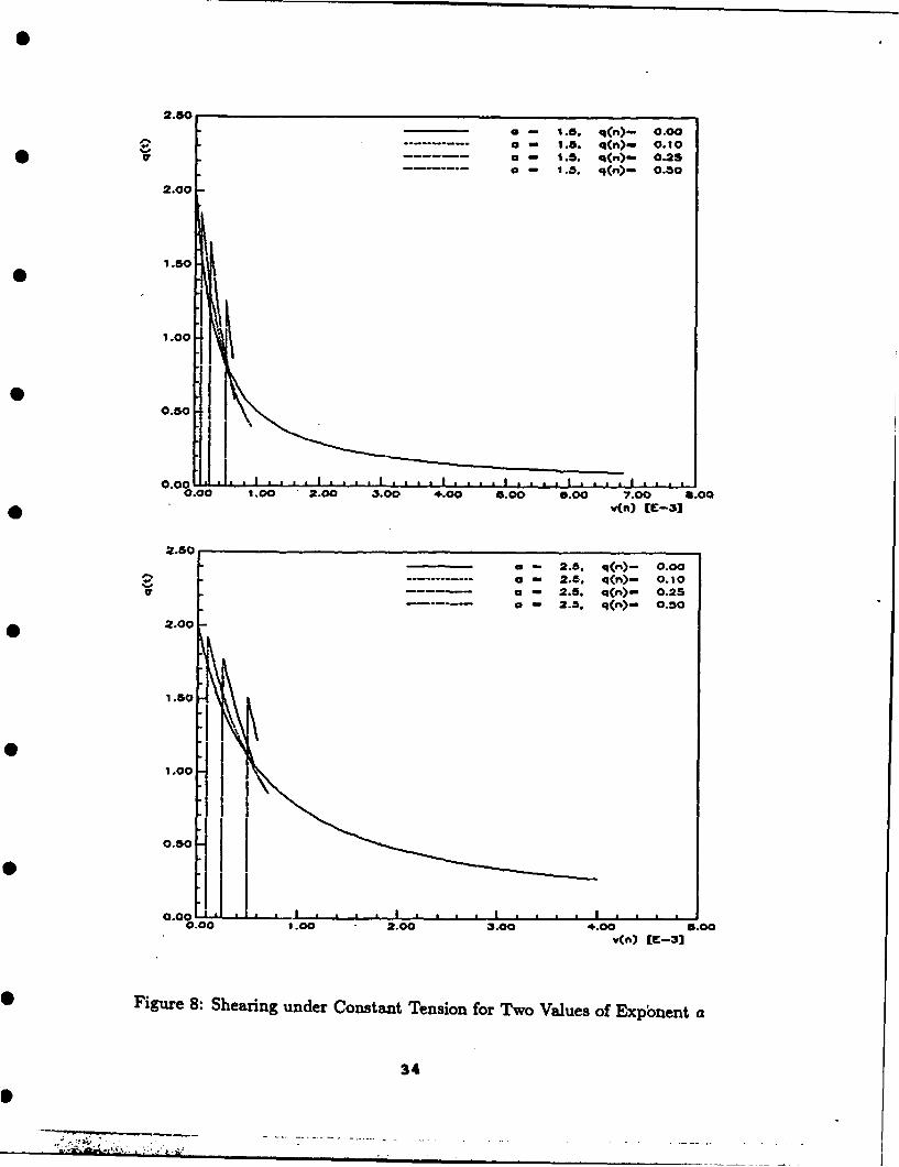
Fig. 8 shows the corresponding dilatancy in pure shear as well as for t4 > 0.
For pure shear it is straightforward to find explicitly the relationship between ut and
Un = uPn when t,, = 0. Using the flow rule expressed by Eq. 10 and the expression for
t4 in Eq.( 22), we obtain
U fn ln (1- f it (25)unu
11

It is seen that u. = 00 when ut = uP = at as shown also in Fig. 8.
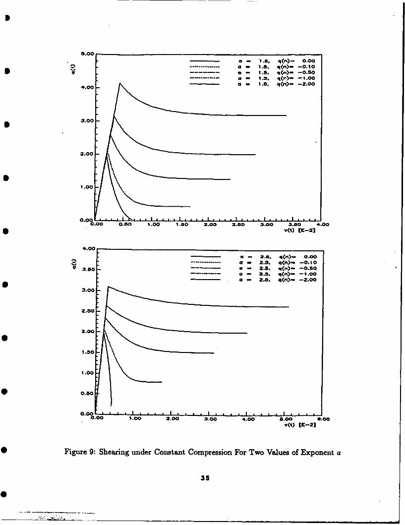
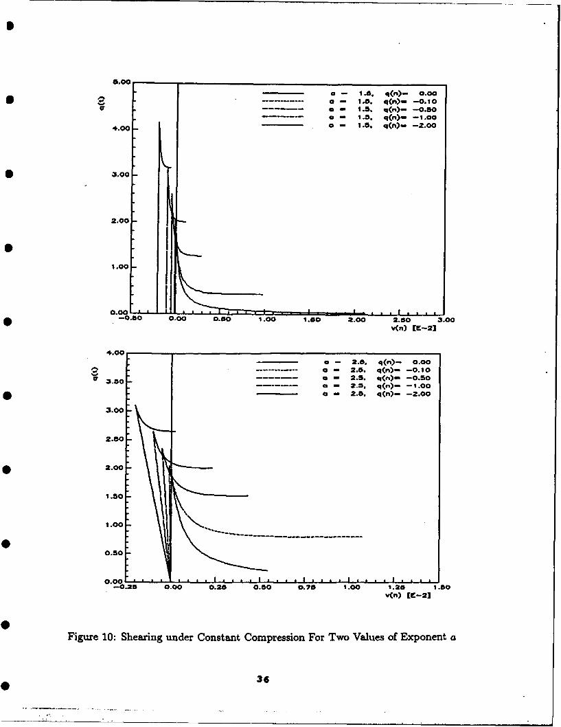
Figs. 9 and 10 show the behavior for compressive contact stress, t. :_ 0. While
tt approaches ft,, asymptotically for large amounts of slip (except in the special case
when t, = 0), the dilatancy displacement uP. is finite at the residual load level (except
when t, = 0) as shown in Fig. 10.
A final comment on the (in-) validity of the assumption that p is constant may
be appropriate. There seems to be experimental evidence that the behavior in shear
depends on the two competing processes that may be described as adhesional soften-
ing and frictional hardening. The former process is treated in the theory described
previously, while it would be possible to simulate frictional hardening by assuming
that the internal friction p is an increasing function of K, i.e. Ji.(tc)/d > 0. The
explicit choice of this functional relationship depends on the roughness of the contact
surfaces. For successively increasing t, the released energy is expected to decrease
until a transition point is reached after which the response will be entirely hardening.
5 UNIQUENESS OF RESPONSE - BRITTLE
BEHAVIOR
It is shown in Fig. 7 that totally brittle behavior was obtained before the shear
strength was completely exhausted for constant t, > 0, while this phenomenon seems
not to occur in pure shear (when t,, = 0). It is possible to obtain completely brittle
response also in pure tension depending on the assumed shape of the relation be-
tween f, and uP and provided that either K or Gf is sufficiently small. However,
such brittleness would occur immediately post peak. Subsequently, we shall inves-
tigate the possibility that the response becomes non-unique under mixed control of
displacements and tractions within the framework of elastic-plastic behavior.
It will be assumed that tl and u2 are the control variables, where tj may be either
t, or tt, whereas u2 plays the role of either ut or U. The relationship in Eq. 5 may
12

then be rearranged as
ei ] = [ K 0 (26)
The consistency condition < 0 can be written explicitely as
OnFi + n2i2 + -F-_c < 0 (27)
where
ni = OF i= 1,2 (28)
From the work-softening hypothesis 12 and the flow rule 11 we obtain
i= sTm (29)
where
s = [< tn >, k(tt - ft,.)]T (30)
and where the flow direction m is given by Eq. 11. Inserting the expression (29) into
the condition (26), we can rewrite the condition (27) in terms of the control variables
tl and u 2
F = n1f, + n 2K2 ti2 - (H + n 2K 2M2 ) < 0 (31)
where H is the generalized hardening modulus
H = OFT
ax
(ft,,)*__ <.tn.> (fg,,) o + k (I tt - I ft,,r ) a 1 1-i] (32)
GI A'g. V
It is noted that the expression (32) is independent of the particular choice of control
variables.
Introducing the 'plastic modulus' K under mixed control
K = H + n 2K 2m 2 (33)
13
and the 'loading function' q
=n ii + n2 K2 i2 (34)
we may rewrite the condition 31 as
P = 4- A K < 0 (35)
The general loading criterion for elastic-plastic behavior is conveniently given in terms
of the Kuhn - Tucker conditions
A> O, P < O, A)P = 0 (36)
and, consequently, from these criteria and 34 we obtain
=/K > O (P) , 4y< 0 (N,E) (37)
where P stands for plastic loading, while N and E denote neutral loading and elastic
unloading respectively. The requirement for a non-ambiguous loading criterion, i.e.
that the loading cases (P) and (E) are mutually exclusive in terms of the value of
0, is that K > 0. This requirement is necessary and sufficient to assure a unique
response for the chosen mixed mode of control.
From Eqs. 26 and (37) the tangent relationship in plastic loading can now be
established in the form
1i K1I mn miK, n2 il 38i] 0 =[-2K 2nj -2K 2])[ ] (38)
or, in compact form,
k=E*, E= E + -k m* n"T (39)
where
X=[] Y=[] n= (40)U2 M21 t2 M -K~m K2n2
In order to investigate the characteristics of the constitutive relation (39), espe-
cially with regard to the possibility of completely brittle behavior, it is illuminating
14

to first establish the spectral properties of E. In fact, brittle behavior corresponds to
(at least) one eigenvalue of E being infinitely large. It is then convenient to consider
the special eigenvalue problem
E x(0 =) ( Ee x (') (41)
It can be shown easily, c.f. Runesson et al. (1989), that one eigenvalue is
AM = 1 + nET n* H+nKjmj (42)T H +n 2K 2M2
corresponding to the eigenmode
x( ) = a (E)-[ m* = a Ki ], a = scalar (43)
The second eigenmode X() is orthogona to n" corresponding to the unit eigenvalue
A(2) = 1. In fact, x(2) defines neutral loading since we have
n*Tx( 2) = n1 i(2) + n 2 K 2 ji(2 ) ' = 0 (44)
In order to avoid brittle behavior, i.e. AM) 0 -0o, for arbitray mixed control, it
follows from Eq. 42 that we must require K > 0. This condition was established
previously as the condition for non-ambiguous plastic loading.
Consider first the case of pure tension, i.e. t,(= U2) changes while tt(= t) = 0.
Since t, _ 0, we obtain ft,, = 0 from Eq. 20, and H becomes
H= (ft,,)2 a tn(
and, so, the condition K > 0 becomes
Kn-t.f9 > 0 (46)
The most critical situation occurs when t. = f,,,u, i.e. at the onset of tensile debond-
ing, which implies that the criterion for unconditional uniqueness of the entire re-
15

sponse function in pure tension is
K, > Uf. )2 (47)
This condition can also be obtained in a more direct fashion by differentiating the
basic relation (15), invoking the elastic portion and imposing the condition that the
total compliance relating ii,, and i, does not vanish. Clearly, the condition (47)
corresponds entirely to the one asssociated with the "smeared fictitious crack" model
for an equivalent continuum; see Ottosen (1986) and Willam et al. (1985).
Consider next the case that t,(= ti) > 0 is fixed while ut(= U2 ) is assumed to
vary in a prescribed fashion. In this case, since t _> 0, it follows that
H=- (f, t ) (it, kap ,6) (8GU 1 (ft,u)a + -a I qt(4
and, so, the condition K > 0 becomes
I t, 12 a-2 (f') q " - Vt (ftu) 2a
agtGf I qt pa2f, G > 0 (49)
In the special case of pure shear, t,, = 0, we obtain the condition
Itt Ia-2 a > 0 (50)a Kt i
If 1 < a < 2 the most critical situation appears for I tt J= ft,u, which gives the
condition for a unique response curve
Kt > (f,,)_2 (51)a GII
If a > 2 the condition 51 can never be satisfied for the entire response curve whatever
parameter values are chosen. Completely brittle behavior is obtained when
0 lit I ( (fti)ftU = a Kt Gi'f (52)
16
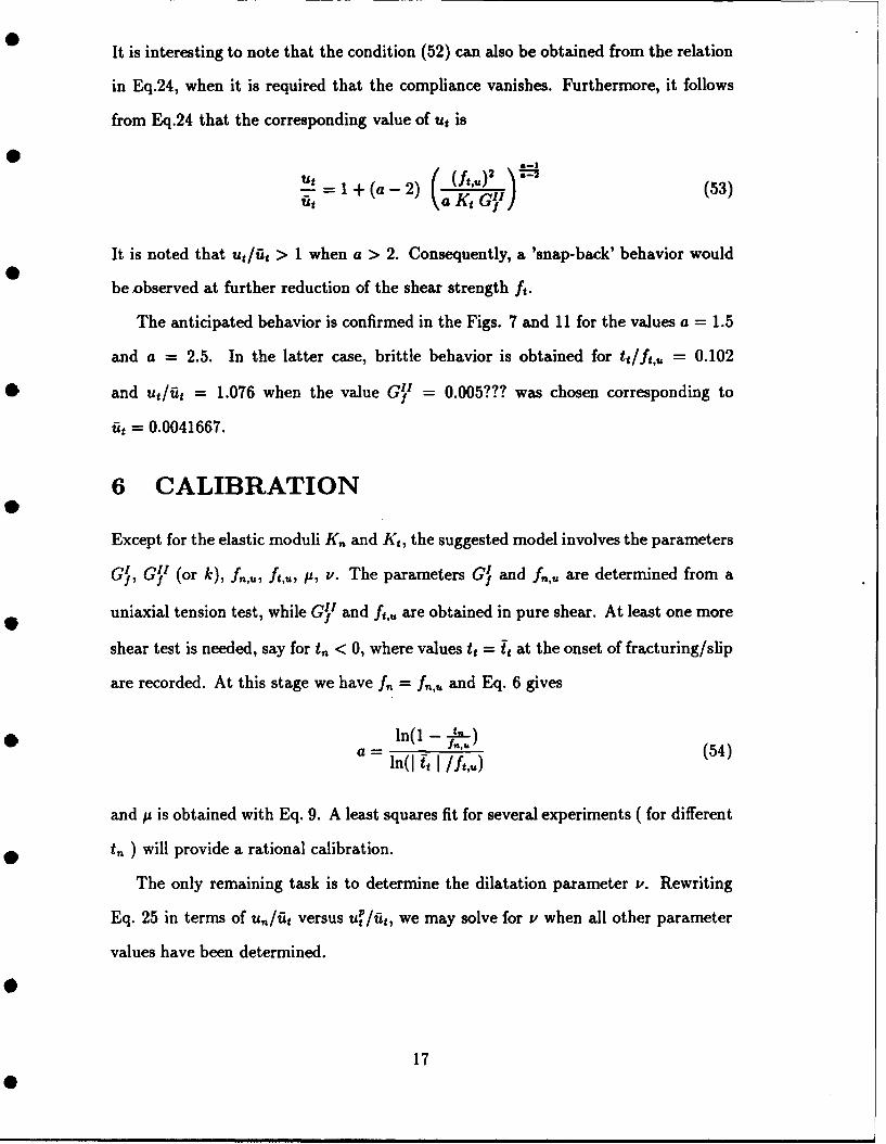
It is interesting to note that the condition (52) can also be obtained from the relation
in Eq.24, when it is required that the compliance vanishes. Furthermore, it follows
from Eq.24 that the corresponding value of ut is
it =1+(a-2) (ft'u)2 (53)a Kt G11
It is noted that ut/fit > 1 when a > 2. Consequently, a 'snap-back' behavior would
be observed at further reduction of the shear strength ft.
The anticipated behavior is confirmed in the Figs. 7 and 11 for the values a = 1.5
and a = 2.5. In the latter case, brittle behavior is obtained for tt/ft., = 0.102
and ut/iti = 1.076 when the value G I = 0.005??? was chosen corresponding to
t = 0.0041667.
6 CALIBRATION
Except for the elastic moduli K and Kt, the suggested model involves the parameters
G1, G11 (or k), f.,u, ft.u, p, v. The parameters Gf1 and f,, are determined from a
uniaxial tension test, while G 11 and f t , are obtained in pure shear. At least one more
shear test is needed, say for t,, < 0, where values tt = it at the onset of fracturing/slip
are recorded. At this stage we have f, = f, ,, and Eq. 6 gives
* ln(l - f (54)ln(I it I//,,)
and y is obtained with Eq. 9. A least squares fit for several experiments ( for different
t" ) will provide a rational calibration.
The only remaining task is to determine the dilatation parameter v. Rewriting
Eq. 25 in terms of ui/t versus uf/'it, we may solve for v when all other parameter
values have been determined.
17

7 APPLICATION
The predictive capabilities of the proposed constitutive theory are compared to two
kinds of experiments. In the first category, the interface is physically represented
by a mortar joint between two masonry bricks, which are displaced relative to one
another. Details of the experiment are described by Attkinson (1989) and the setup
is schematically illustrated in Fig. 11. In this form of experimental arrangement it
*1 is reasonable to assume that the observed deformations are confined to the mortar
layer since the bricks are superior in strength and stiffness by at least one order of
magnitude compared to the masonry mortar. Fig. 12 shows the analytical load-
displacement predictions of the constitutive model and the experimental results for
three levels of constant normal compressive load. In these particular experiments
the normal stress was maintained at a constant level while the shear was applied by
controlled tangential displacement.
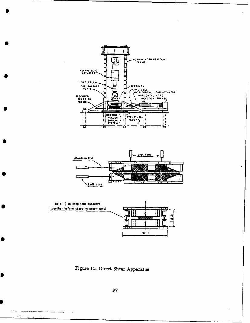
The second set of experimental results were obtained from pilot studies currently
performed at the University of Colorado, in which mortar-aggregate interface charac-
teristics are investigated. In these experiments, the mortar is represented by a con-
crete mix in which particles with a diameter larger than 2.8 mm have been omitted.
The aggregate is represented by a 6.0 mm thick granite plate or disk whose surfaces
have been carefully treated by sandblasting to ensure uniform and competent bonds
with the adjacent mortar. A mortar disk having 50 mm diameter and a uniform thick-
ness of 25 mm is cast directly on this granite plate, which have been glued to a base
aluminum plate with structural epoxy. Several granite disk - aluminum base assem-
blies have been manufactured to test various series of mortar-granite interfaces. After
curing, the specimen is placed into a direct simple shear apparatus, and a aluminum
top plate that is mounted in a loading frame, is glued in situ to the top surface of the
mortar disk. The vertical loading frame allows the application of normal compressive
or tensile loads. Shearing is applied by controlled displacement of the base assembly
sledge system on which the base aluminum plate has been mounted. A previously
18
mentioned the vertical load was kept constant during the experiments. However, due
to inadequate stiffness of the test apparatus, a stable post-peak response was not
obtained, and clearly, the degree of instability increases as the normal compression
* increased.
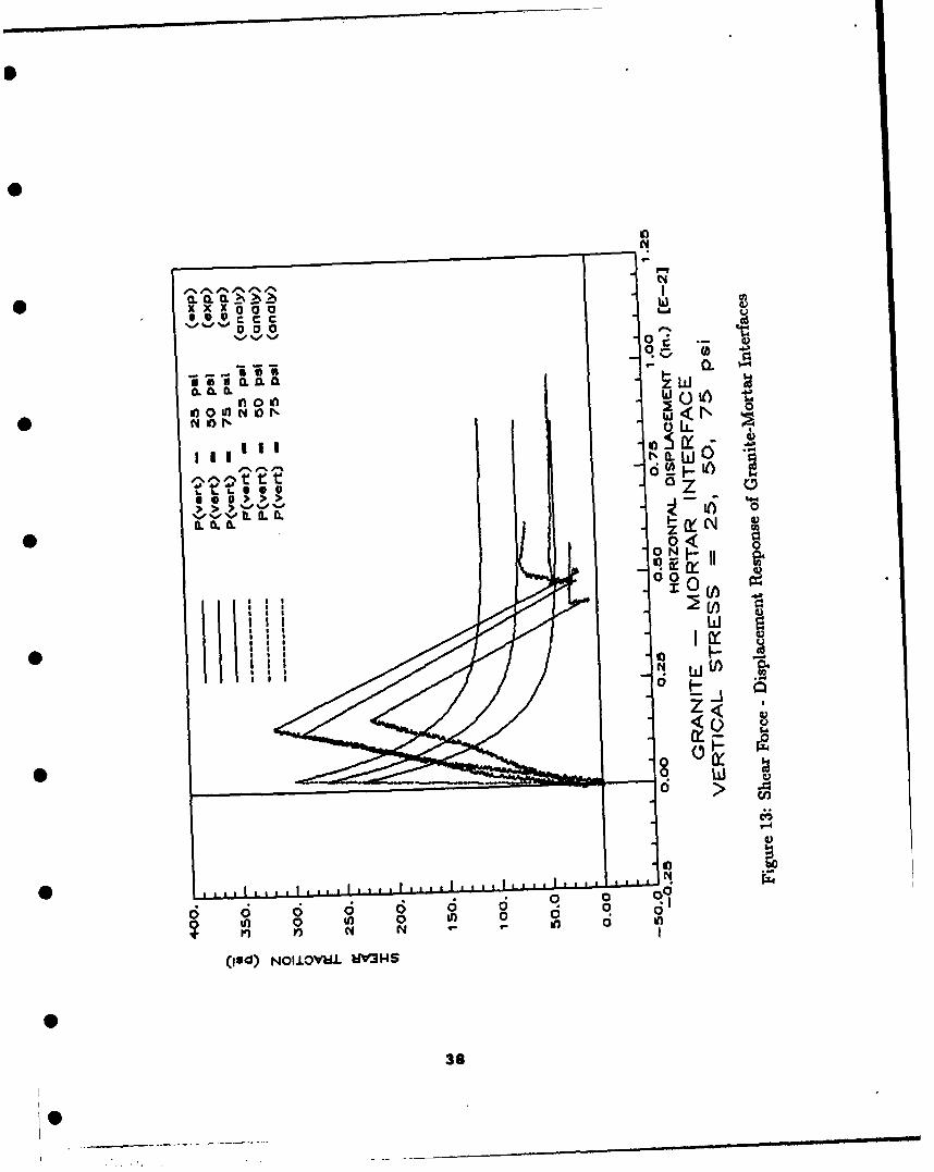
Fig. 13 shows the obtained results along with the analytical predictions of the
proposed model at the constitutive level. The displayed horizontal displacements are
relative displacements between the top and base aluminum plates. Since the granite
plates are far stiffer than the mortar, the measured displacements reflect essentially
the deformation of the interface and the mortar, except at the residual strength after
the interface has failed. From these considerations, it has to be concluded, that the
interface properties during loading and softening have to be determined from a in-
verse identification procedure, in which the entire specimen is modeled as a miniature
structure and realistic boundary condition are applied, as illustrated in Fig. 14.
ACKNOWLEDGEMENTS
The authors gratefully acknowledge the financial assistance provided by Grant AFOSR-
89-0289 and the support of Dr. Spencer Wu.
8 APPENDIX I: REFERENCES
Atkinson,R.H., Saeb,S, Amadei,B., Sture,S. (1989)," Response of Masonary Bed Joints
in Direct Shear", ASCE J. Struct. Eng., Vol. 115, No. 9, pp. 2276-2296
Chandra,S. (1969), "Fracture of Concrete under Monotonically Increasing, Cyclic and
Sustained Loading", Ph.D. Thesis, Dept. CEAE, University of Colorado, Boulder,
Colorado
Gilette,D., Sture,S., Ko,H.-Y., Gould,M.C., Scott,G.A. (1983),"Dynamic Behavior of
Rock Joints", Proc. 24th U.S. Symposium on Rock Mechanics, Texas A & M Univ.,
1983 pp. 163-179.
19
Glemberg,R. (1984),"Dynamic Analysis of Concrete Structures",Dept. of Struct.
Mech., Publ. 84:1, Chalmers University of Technology, Gothenburg, Schweden
Goodman, R.E. (1980),"Introduction to Rock Mechanics", John Wiley & Sons, New
York, N.Y.
Nilsson,L., Oldenburg,M. (1984),"Nonlinear Wave Propagation in Plastic Fracturing
Materials - A Constitutive Modelling and Finite Element Analysis",
IUTAM Symposium: Nonlinear Deformation Waves, Tallin 1982, Springer Verlag,
Berlin 1982, pp. 209-217
van Mier,J.G.M, Nooru-Mohamed,M.B. (1988),"Failure of Concrete under Tensile and
Shear Like Loadings", Int. Workshop on Fracture Toughness and Fracture Energy-
Test Methods for Concrete and Rock, Oct.12-14,1988, Tohoku University, Sendai,
Japan
Ottosen,N.S. (1986),"Thermodynamical Consequences of Strain-Softening in Ten-
sion", J. Eng. Mech., ASCE, Vol. 112, No. 11, pp. 1152-1164
Plesha,M.E., Haimson,B.C. (1988),"An Advanced Model for Rock Joint Behavior:
Analytical, Experimental and Implementational Considerations", Proc. 29th Symp.
on Rock Mechanics
Plesha,M.E., Ballarini,R., Parulekar,A., (1989),"Constitutive Model and Finite Ele-
ment Procedure for Dilatant Contact Problems", ASCE J. Eng. Mech., Vol. 115,
No. 12, pp. 2649-2668
Roelfstra,P.E., Sadouki,H., Wittmann,F.H. (1985), "Le B1ton Numdrique",
Materials and Structures, RILEM, Vol. 118, No. 107, pp. 309-317
Runesson,K., Mroz,Z. (1989),"A Note on Non-Associated Plastic Flow Rules", Int.
J. Plasticity, Vol. 5, pp. 639-658
Shah,S.P., Sankar,R. (1987),"Internal Cracking and Strain Softening Response of
Concrete under Uniaxial Compression",Report Center of Concrete and Geomaterials,
Technological Institute, Nothwestern University, Evanstone, II.
Stankowski,T. (1990) Numerical Simulation of Progressive Failure in Particle Com-
posites, Ph.D. Thesis, C.E.A.E. Department, University of Colorado, Boulder, Col-
20

orado Willam,K., Bicanic,N., Sture,S. (1984),"Constitutive and Computational As-
pects of Strain-Softening And Localization in Solids", ASME/WAM 1984 Symposium
on Constitutive Equations, Macro and Computational Aspects, (Ed. K. Willam),
ASME Vol G00274, New York, N.Y., pp 233-252
Willam,K., Pramono,E., Sture,S. (1985),"Stability and Uniqueness of Strain-Softening
Computations",Europe - U.S. Symposium on Finite Element Methods for Non-linear
Problems, (Eds. Bergan, Bathe, Wunderlich), Springer Verlag, Berlin, pp. 119-142
Willam,K.J., Stankowski,T., Runesson,K., Sture,S. (1988)," Simulation Issues of Dis-
tributed and Localized Failure Computations", France - U.S. Workshop on Strain
Localization and Size Effect Due to Cracking and Damage, ENS Cachan, France,
(Eds Mazars and Baiant, Elsevier Appl. Science, pp. 363-378
9 APPENDIX II: NOTATION
A = trrsformation matrix
a = exponent of fracture/slip function
C = compliance matrix
F = fracture/slip function
f = tensile/shear strength
G1, GI I = energy release in tension and shear (material constants)
H = hardening modulus
k = material constant
K,, Kt = elastic normal and tangential stiffness moduli
K= plastic modulus
en, et = normal and tangential base vectors
m = gradient of plastic potential
n = gradient of fracture function
t = vector of contact traction
21

a -vector of effective traction
u = vector of relative displacements
x = eigenmode
I
f = coefficient
= measure of released fracture energy
A= plastic multiplier; eigenvalue (with superscript)
= loading function
= coefficient of friction
v = coefficient of dilatancy
Subscripts
n = normal direction
r = residual strength
t = tangential direction
n, U = initial (ultimate) tensile strength
t, u = initial (ultimate) shear strength
Superscripts
() = rate, differentiation with respectto (pseudo)time
e = elastic
p = plastic
22
9 "PNDIX III
The Construction of Voronoi Polyhedra in Three Dimensions
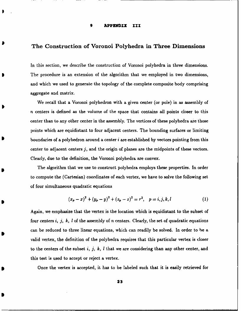
In this section, we describe the construction of Voronoi polyhedra in three dimensions.
The procedure is an extension of the algorithm that we employed in two dimensions,
and which we used to generate the topology of the complete composite body comprising
aggregate and matrix.
We recall that a Voronoi polyhedron with a given center (or pole) in as assembly of
n centers is defined as the volume of the space that contains all points closer to this
center than to any other center in the assembly. The vertices of these polyhedra are those
points which are equidistant to four adjacent centers. The bounding surfaces or limiting
boundaries of a polyhedron around a center i are established by vectors pointing from this
center to adjacent centers j, and the origin of planes are the midpoints of these vectors.
Clearly, due to the definition, the Voronoi polyhedra are convex.
The algorithm that we use to construct polyhedra employs these properties. In order
to compute the (Cartesian) coordinates of each vertex, we have to solve the following set
of four simultaneous quadratic equations
(xP - x) 2 + (Yp _ y) 2 + (zp -z) 2 = r2 , p= i,j,k,l (1)
Again, we emphasize that the vertex is the location which is equidistant to the subset of
four centers i, j, k, I of the assembly of n centers. Clearly, the set of quadratic equations
can be reduced to three linear equations, which can readily be solved. In order to be a
valid vertex, the definition of the polyhedra requires that this particular vertex is closer
to the centers of the subset i, j, k, I that we are considering than any other center, and
this test is used to accept or reject a vertex.
Once the vertex is accepted, it has to be labeled such that it is easily retrieved for
23
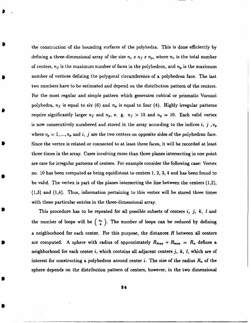
the construction of the bounding surfaces of the polyhedra. This is done efficiently by
defining a three-dimensional array of the size n, x nx x np, where n, is the total number
of centers, nf is the maximum number of faces in the polyhedron, and np is the maximum
number of vertices defining the polygonal circumference of a polyhedron face. The last
two numbers have to be estimated and depend on the distribution pattern of the centers.
For the most regular and simple pattern which generates cubical or prismatic Voronoi
polyhedra, nf is equal to six (6) and np is equal to four (4). Highly irregular patterns
require significantly larger nf and nrp, e. g. nf > 15 and np = 10. Each valid vertex
is now consecutively numbered and stored in the array according to the indices i, j ,vp
where vp = 1, ..., nP and i, j are the two centers on opposite sides of the polyhedron face.
Since the vertex is related or connected to at least three faces, it will be recorded at least
three times in the array. Cases involving more than three planes intersecting in one point
are rare for irregular patterns of centers. For example consider the following case: Vertex
no. 10 has been computed as being equidistant to centers 1, 2, 3, 4 and has been found to
be valid. The vertex is part of the planes intersecting the line between the centers (1,2),
(1,3) and (1,4). Thus, information pertaining to this vertex will be stored three times
with these particular entries in the three-dimensional array.
D This procedure has to be repeated for all possible subsets of centers i, j, k, 1 and
the number of loops will be ( nc ). The number of loops can be reduced by defining
a neighborhood for each center. For this purpose, the distances R between all centers
are computed. A sphere with radius of approximately R,, + Ri,, = R, defines a
neighborhood for each center i, which contains all adjacent centers j, k, 1, which are of
interest for constructing a polyhedron around center i. The size of the radius R, of the
sphere depends on the distribution pattern of centers, however, in the two dimensional
24

case it has been found to be sufficiently large.
When all vertices are computed, the bounding surfaces or limiting boundaries of the
polyhedra are readily established. The polygon drawn in the surface plane between centers
i and j are the vertices stored in the array i, j, n, n = 1, ..., nP.
The remaining consists of constructing the exterior surfaces of the domain subdivided
into Voronoi polyhedra. This is achieved by first identifying all centers in the vicinity
of the exterior surfaces, e. g. in a distance less than approximately 2 x R,,,.. In this
second step we consider these centers i and only two other sets of centers j and k in
their neighborhoods. The center(s) i is reflected on the exterior surface defining a point
i' outside of the material. Three centers i, j, k form now together with point i' a subset
from which a vertex can be computed as described above. Since this vertex is on the plane
intersecting i and i', it will be on the exterior surface. This vertex is stored only once in
the three-dimensional array with the entry i, i'. Again, this loop has to be repeated for
all centers in the vicinity of the material surfaces.
* The algorithm can be summarized as follows:
1. Compute the distances between all centers, n, of the assembly and define the size
of the neighborhood.
*0 2. Identify for each center, i, those centers that are in the neighborhood, and which
are relevant for the construction of the polyhedron around the center i.
3. Compute the vertices around each center, and check the validity of using the centers
in the neighborhood and store them in a three-dimensional array.
4. Identify those centers which are close to the bounding surface of the domain con-
sidered.
25
5. Compute the vertices on the bounding surface, test them for their validity, and store
the relevant information.
After completing the computations of the vertices, the topology of the polyhedra is
completely defined within a three-dimensional array. The index i defines the polyhedron
and together with index j the bounding surfaces of the polyhedron are labeled. The points
with indices i, j, k, 1 = 1,...np define a polygon enclosing in the bounding surface i, j.
In the event these polygons do not close, the size of the neighborhood has to be increased.
Reference
Finney, J. L. "A Procedure for the Construction of Voronoi Polyhedra", J. Cornp. Physics,
1979, Vol. 32, pp. 137-143.
26
0 :1
0
43
0
*0~
4)
1'40
4.4
0*
.2
-4-' -
S U -8-4 ___
-4-,L2
S
S
27
S
4E-
.0-
z
0-0
28
.....S.. .
S0
E I
>005
>000
>004
>00)
C44
29
29
7 " . . . . ... .. .. .
40
4-o
(D C)
30U
.2
o q).
-4.,.
0
0
v I -o
II ,_V
* .o.
II *. I -
* . I,\. 'oCr
I)
o3
.*.. ." - " ' " . . . .. . . •U' : .'
2.5
2.00a - Sq(n)- 0.00
......... - .0. q(n)- 0.108 - .5. q(n)- 0.25
* a- 1.3. q(n)- 0.50
2.00-
0 1.0
final value
0.00 1.00 2.0,0 3.00 4.00 5.00 6.00 7.00 a 00
2.0a -2.8. q(n)- 0.00
------- a. 2.5. q(n)- 0.10a-2.5. q~n)- 0.25
- ~ ---- 2.3. q(n)- 0.50
0 2.00-
1.00-
0.0
* theoretical limit
0.00 500.00 1.00 2.00 3.00 4.00 5.00E-3
* Figure 7: Shearing under Constant Tension for Two Values of Exponent a
33
S
2.50a ,,- i.e. q(n)- 0.00
--- ----- 1.. q(n), 0.10* v a - 1.5. q(n)- 0.2S
a - 1.5o q(n)- 0.30
2.00-
1.50
1.00
0.50
0.000.00 1.00 2.00 3.00 4.00 5.00 0.00 7.00 0.00
v(n) [E-31
2.80
a - 2~.6. q(n)- 0.00-------- - - 2.6. q(n)- 0.10
0 - 2.5. q(n)m 0.25. w 2.5, q(") - .0
2.00
1.80- '1.00
II 10.50
0.00 ,I _ _ _ _ _ _
0.00 1.00 2.00 3.00 4.00 .00
v(n) [rS]
Figure 8: Shearing under Constant Tension for Two Values of Exponent a
34
- ' - .. . .... . . ...... .. .
0.00
'i- .e. q~n)- 0.040.. ....-- a m 1.0. q(n)- -0.10
a I .5. q(n- -0.50a-1.5. q(u-)- -1.00
4.00- a I .e. q(n)- -2.00
S 3.00
2.00-
0.00 0.50 1 .00 1.50 2.00 2.0 3.00 3.50 4.00*v(t) EIE-21
+.00
a 2.0. q(n)- 0.C0---------- a 2.6. q(n)- -0.10
3.50-- - a -2.5. q(n)in -0.50- ----- - 2.5. q(n).. -1.00
a-2.0. q(n)- -2.00
3.00-
2.50-
2.00
0.00 1.00 2.00 3.00 4.00 5.00 6.00vWt [E-23
0 Figure 9: Shearing under Constant Compression For Two Values of Exponent a
35
5.00
a - 1.5. q(n)- 0.00. - 1.5. q(n)- -0.10
S- 1.5. q(n),- -0.50a -- 1.- q(n)- -1.00
4.00 1. q(n)- -2.00
3.00
2.00
1.00
0.00 1'I .- -,
--0.50 0.00 0.50 1.00 1.50 2.00 2.60 3.00
v(n) [E-23
4.00a - 2.5. q(n)- 0.00
...-.. . a ,, 2.6. q(n)- -0.10
3.50 a - 2.5. q(n)- -0.50..0.... a - 2.5. q(n)- -1.00
a - 2.5. q(n)- -2.00
3.00
2.80-
2.00-
1.50-
1.00 -- - --
, I
0 0.00-o.25 0.00 0.26 0.50 0.76 1 .0o 1.25 1 .50v n) [r-2)
Figure 10: Shearing under Constant Compression For Two Values of Exponent a
36
S ,"
SZ
~ ~.NOML LOAD REACTION
NORMAL LOADACTUATOR
LOAD CELL
WCUIZONT"L LOAD ACTUATOR
I:BOTTOMRtOLLER .. *----,
SSE
Fluiume Ro:dirc ha paau
P" .MS .M
\L~dt co7
Bot T epsaoeodr
00
0
-6 0 CCw
0- 0I
e L)N 00.0
0 06
gel> >'-
*0<
00
<0-
00
r-4
N 0 0
00
38

400.
S350.-
00.* 250. .. Aayi
200.
50.0-
0.00
-0.25 0.00 0.25 0.50 0.75 1.00 1.25HORIZONTAL DISPLACEMENT (in.) [E-21
GRANITE -MORTAR INTERFACEVERTICAL STRESS =75 Pal
M ~oirtarDeformation at Peak
GrSt
- -- -Deformation at Residual Strength
Figure 14: Structural Simulation of Granite-Mortar Interface
39
* FRACTURE AND SLIP OF INTERFACES
IN CEMENTITIOUS COMPOSITES
Part 11: Model Implementation
by
0 T. Stankowskil, K. Runesson 2, S. Sture3
1Res. Assoc., Dept. of Civil, Environmental, and Architectural Engrg., University of Colorado,Boulder, CO 80309.
2Visit.Prof., Dept. of Civil, Environmental, and Architectural Engrg., University of Colorado,* Boulder, CO 80309.
3Prof., Dept. of Civil, Environmental, and Architectural Engrg., University of Colorado, Boulder,CO 80309.
Contents
1 INTRODUCTION 3
2 INCREMENTAL RELATIONS 32.1 Implicit Integration ............................ 32.2 Newton Iteration ............................. 52.3 Interpolation/Iteration Scheme ..................... 62.4 Iterative Procedure for Mixed Control .................. 8
3 FINITE ELEMENT MODELLING WITH INTERFACES 83.1 Basic Equations .............................. 8
'3.2 Iterative Scheme - Numerical Performance ............... 10
4 NUMERICAL RESULTS 12
5 SUMMARY AND CONCLUSIONS 13
6 APPENDIX I: ALGORITHMIC TANGENT STIFFNESS 15
7 APPENDIX II: EXTENSION OF THE MODEL TO THREE DI-
MENSIONS 17
8 APPENDIX III: REFERENCES 18
9 APPENDIX IV: NOTATION 19
2
1 INTRODUCTION
In Part I of this paper we developed a constitutive theory for fracture and slip of inter-
faces in cementitious composites. The characteristic behavior that can be predicted
with this constitutive theory was analyzed, and limited comparisons with experimen-
tal results obtained from shear tests under constant normal load were presented. In
the present Part II we discuss the numerical techniques that are employed for integrat-
-0 ing the constitutive relations of the interface. The fully implicit method, or Closest
Point Projection Method (CPPM) is chosen as the 'core-alogorithm' that employs a
displacement-driven scheme. A robust iterative technique is devised for solving the
nonlinear incremental problem of calculating the contact stresses or tractions in the
interface, which is essential for the successful implementation in a fin;fe element anal-
ysis code. We also use a scaled gradient iteration technique for the solution of the
incremental finite element problem, which requires the development of the appropri-
ate Algorithmic Tangent Stiffness matrix. This matrix can, in fact, be used to assess
the stability of the actual incremental solution. Finally, finite element results are
presented for pertinent boundary value problems.
0
2 INCREMENTAL RELATIONS
2.1 Implicit Integration
By combining Eqs. 2, 4 and 10 of Part I, Stankowski et al., we obtain the constitutive
relationship between the interface tractions and relative displacements. These rela-
tions define together with the hardening rule in Eq. 29 and the fracture/slip criterion
in Eq. 6, Part I, the complete set of constitutive relations for the behavior of the
interface:
6=Cet + m(t) (1)
ic = sT(t) m(t) (2)
F(t,ic) = 0 (3)
30
A number of different techniques for integrating these relations are available. The
Generalized Trapezoidal Rule (GTR) has been evaluated by Stankowski (1990), and it
was concluded that the most robust scheme should be based on a fully implicit inte-
* gration scheme, which is a special case of the GTR-method. In this paper we employ
a slightly modified version of the implicit method (CPPM), which has been developed
by Runesson et al.(1988), whereby the modification concerns the integration of the
softening variable in Eq. 2. Since the current yield surface F = 0 is always convex
for'a given value of oc, integration according to the CPPM guarantees the existence
of a stress solution in terms of a projection property.
Using the modified CPPM we may integrate Eqs. 1 and 2 to obtain, for 0 _ 5 _5 1,
+lft - n+lte- ADe n+lm (4)
n+lK = 'C + A n+I-sT n+lm (5)
n+IF = 0 (6)
where n(.) denotes the current state at time t = nt, whereas "+'(.) denotes the
updated or unknown state. The trial (elastic) traction n+1 qe is defined as
n+lte = nt + D e Au, De = (Ce)- 1 (7)
Furthermore, we have used the notation
n+lm = m (+lt) , n+IF F (n+lt, n+1K) (8)
n+s = s(n+vt) , "+ t=(I nt+-n+lt (9)
A variety of different techniques is available for the solution of Eqs. 9 for a given trial
stress n+lte, either by a pure iteration scheme or a combined iteration/interpolation
technique.
4
2.2 Newton Iteration
The most 'direct' approach is to use a Newton Iteration Scheme in order to calculate
n+lq and n+1,C simultanously from Eqs. 9, whereby the current fracture/slip surface
is updated at each iteration. It was shown by Stankowski (1990) that for this scheme
to converge requires that the initial values are carefully chosen. Moreover, it is in-
creasingly difficult to choose the initial values as the size of the load increments Au
increase, i.e. when n+lte is far away from the initial fracture/slip surface 'F. The
performance of the iteration scheme is significantly improved, if the stress projection
inferred by Eq. 4 is performed for a fixed surface, whereby n+lt and A are simultane-
ously calculated from the following equations:0
g(n+'t, A) = de (n+It _ ,+lte) +An (-+'q) = 0 (10)
* ~ F~f+lt F ,) = 0 (1
where ce = A-' Ce and A is the transformation matrix in Eq.(11) of Part I account-
ing for non-associated flow due to dilatancy properties of the interfcae. The structure
of Eq. 11 is simple since, in fact, tC is diagonal.
Newton iterations to solve for n+lt and \ from Eqs. 11 and (11) give for the
iteration step (.)i+':
n+lt(i+l) = n+lt(i) + dt, 0(+1) = 0) + dA (12)
where the improved values dt and dA are calculated from the set of equations
&+AN n]W dt ] - [0) f ] (13)
The matrix N is the Hessian of f, i.e. N 0 02f/Ot Ot.
As indicated earlier, it seems to be essential to use good initial solutions n+lt(°)
and AM(0) in order to ascertain that the scheme has efficient and reliable iteration
405
properties. For relatively small steps, it has proved efficient to calculate the predictor
from forward extrapolations in Eq. 9 with 8 = 0. The solution is conveniently found
by calculating A() from
f (A(° )) = F (n+it(o), u+iK(O)) (14)
where
n+lt(-) = +lte - A() D e nm (15)
n+1r(0) - nK + A(O) isT n m (16)
Since only an initial solution is sought, it is sufficient to find only an approximate
solution of Eq. 14 with a limited number of iterations.
2.3 Interpolation/Iteration Scheme
For increasingly larger increments the quality of the predictor becomes a crucial issue
for the success in efficiently solving the set of constitutive equations given in Eqs. 10
0 and (11). This is in particular the case, when the stress is projected onto a region
of the fracture surface F = 0 with strong curvature, and when a significant change
in the softening variable K is encountered. In fact, the predictor obtained from a
forward extrapolation outlined in the previous section, proved to be sufficient only40
when the magnitude of the elastic traction n+lte, which reflects the increment size,
was of the same order as the elastic limit fu. However, since it can be anticipated
that slip and debonding occur in a rather brittle fashion close to structural failure
* with significant relative motion in the interface, it is essential to deal with elastic trial
stresses n+lte whose magnitudes are several orders larger than fn,u. In order to find a
solution of Eqs. 10 and (11) for these cases, an alternative technique was developed
that employs a quadratic interpolation scheme for the calculation of n+lt when F = 0
is maintained constant.
6
The projection of the elastic trial stress n+Ite onto the current slip surface F(U) = 0
is carried out by solving the orthogonality condition
dT tF = 0 (17)
whered = Ce (te - 0~)) (18)
* and tF is the tangent to the plastic potential in t(). This condition is equivalent to
finding the minimum distance d in strain space for the case of associated flow. For
non-associated flow C' in Eq. 18 has to be transformed. The orthogonality condition
in Eq. 17 has been chosen, since it is more suitable for the interpolation scheme
employed. Alternatively, the stress projection could be carried out by minimizing
II d II. An initial interpolation interval is readily established for example by the
projections of n+lte parallel to the tangential and normal directions on F(U) and
t0 _< fn. If qn > q,,f, then the initial interpolation interval is established by the
projection of n+ltt in the normal direction on F(U) and by fn. The intermediate
pivot is taken at the midstep. Subsequent surface updates have to be monitored very
carefully, since initial updates may result in
n+lr('+') > G1 (19)
In this case, the motion of the surface has to be restricted by assuming
= a (G1 - n.) (20)
where a* is a factor, e.g. 0.5. As the iterations proceed, AKc decreases and will
eventually become
n+lr(i+i) < n,+iK(i) (21)
i.e. n+lt(i+l) is inside F such that F(n+lt(i+l), "+11a(i+ 1)) < 0. At this stage, the
values n+10+1) and +1t (i+i) are used in an interpolation scheme to obtain new
values for n+i K. During the surface updates the new interpolation intervals have to
7

be established carefully depending on the motion of the surface. The non-monotonic
behavior arises from the worksoftening assumption and explains the limitation of a
Newton iteration scheme to small step sizes, when the surface is updated at each
* iteration level.
2.4 Iterative Procedure for Mixed Control
Mixed control of one traction and one relative displacement component is readily
dealt with within the framework of the outlined integration-iteration procedures. If
for example, i+lt_ =n+l in is prescribed, then because of the elastic decoupling of
n+t, and +t, the first row in Eq. 4 can simply be deleted, and '+'tn in+ I_
* is inserted in the other equations. When "+1 tt and \ have been calculated (after
convergence of the chosen iteration algorithm), it is a relatively simple matter to
calculate the remaining unknown displacement component Au, (and n+lun) from the
first row in Eq. 6.
3 FINITE ELEMENT MODELLING WITH IN-TERFACES
3.1 Basic Equations
In order to describe the interaction of two constituents across the interface we con-
sider the common boundary r, (interface) that separates the regions 0?P) and Q(2) as
shown in Fig.(1). Apart from the common portion F, the boundary of each region is
composed of a part with prescribed displacements and another part with prescribed
applied tractions. For simplicity, we assume henceforth that the boundary tractions
as well as the body forces are absent.
Vector components are normally referred to global Cartesian coordinates. How-
ever, along the interface it is convenient to resort to normal and tangential compo-
inents. The relative displacement v = U(2) - 0) and the contact traction q = q(1) -
-q(2) at each point along the interface I'c may then be decomposed as in Eqs. 1 and
8

(3) of Part I, where the base vectors e. and eg are attached to the region 00().
At each instant the stresses must satisfy the equilibrium equations in the regions
fl(l) and f0(2). The appropriate virtual work equation at time t = 4,+1 may be written
as
J ((w )T n+lor() dR - jr (00) )T n+lt(i) dl' = , i = 1, 2 (22)
for all (virtual) kinematically admissible displacements ii(i). By adding, formally, the
two equations in (22) we obtain
LE (Y()) T n~a')d + Jr [, +Itd = 0 (23)=1,2
where ii = ii(2) - i(I).
The term of interest for interface modelling is the boundary term in in Eq.(23)
I =I i1T +lt d1 = fr.jO ( +It + iti n+1 t) dl (24)
Since a constitutive relation is available for "+lt n and n+ltt in terms of Aun and Aug,
i.e.
=+t = t(Au) (25)
or, explicitly
+1= t (AU,AU,), ' +ltt = t,(AU, Au )
the boundary integral in Eq.(24) contributes to the global stiffness of the jointed
regions 0(0) and f(2).
Discrete (= finite element) equations corresponding to the virtual work expression
in Eq.(23) are obtained in the usual way via appropriate shape functions, where we
expand the displacement field 0'), i = 1, 2, and the relative displacements u as
u = ()p(-) + ips) u = 4, (p 2) _ (26)
Here, we have introduced 4k as the restriction of 4(, i = 1,2 to the interface re.
9S[
Inserting Eq.(26) into Eq.(23) gives rise to the set of equations
1) (p(),p1)) (p),p2)) 0(27)
9(2) (2), ($2))-r (1), (2)) = 0
S(2) (p(2) P(2) = 0
where we have introduced the nodal forces
S J (B(')j T o (pW,pW))
Li (P 8Cdf
whith the common definition given to the strain-displacement matrices B(') and B~'),
SW= 1,2.
3.2 Iterative Scheme - Numerical Performance
For each time step the incrementally non-linear finite element problem in the set of
equations Eq.(27) involving the interface model is solved by scaled gradient (or modi-
fied Newton) iterations. In the special case of true Newton iterations the Algorithmic
Tangent Stiffness matrix for the composite is used. The contribution relating to the
contact force rC is given as
= C Dc (v) tc dr (29)
where the appropriate formulation of the constitutive matrix of the algorithmic tan-
gent moduli Dc is given in the appendix. In the case there exists a unique solution to
the incremental finite element problem defined by the equations Eq.(27) that corre-
sponds to ther minimum of an incremental potential as discussed by Runesson et al.
10

(1990), Newton iterations will converge to this solution (except in some pathological
cases). However, for softening materials one may encounter unstable solutions that
correspond to insufficiently localized deformation modes, and the solution turns out
to be non-unique. In such a case, the Newton technique fails in general (depending
on the choice of the start solution). A modified stiffness matrix, which is positive
definite, must be adopted in order to ensure convergence to a local minimum, so that
at the very least, an unstable solution can be avoided. (We note that there is still
the inherent difficulty of finding the most stable solution.)
The crudest choice of an iteration matrix in this case, when the Hessian seizes to
be positive definite, is the elastic stiffness matrix corresponding to the initial stress
iteration method. In order to establish a modified stiffness that is closer to the
Hessian, the negative eigenvalues are modified on the constitutive level as explained
in the following.
Consider the eigenvalue problem for the Algorithmic Tangent Operator that is
pertaining to the interface behavior
Dcxi = -fDxi, i = 1,2 (30)
where xi are the De-normalized eigenvectors. It follows that D, can be represented
in terms of its spectral properties as (for the 2D-case)
DC = E Aixix T (31)i=1,2
Whenever A1 < 0, we replace Dc by D* defined as
Dc = 1 Aixixir (32)i=1,2
This choice representing zero stiffness associated with a (local) failure mode resembles
the fully fractured behavior.
The situation that A1 < 0 was indeed encountered in the calculated examples.
With the suggested modified stiffness, the resulting iteration procedure turned out to
be quite efficient.
11
4 NUMERICAL RESULTS
In order to examine the ability of the interface model to mimic the separation of a
single inclusion embedded in a matrix, a panel with a circular inclusion is subjected
to uniaxial tension. Fig. 1 shows the deformed mesh (for a quarter panel, since
symmetry can be exploited) and the load-displacement relation for this structure.
The tensile strength of the mortar matrix was taken to be 20% higher than the
one of the interface (q,,jg). In order to assure that the post-peak load-displacement
relation represents stable behavior under displacement control, i.e. to avoid snap-
back behavior, we must choose the energy release Gf large enough. This may, in fact,
correspond to a rather ductile post-peak response (on the constitutive level). It was
concluded that the interface model can be utilized to capture the progressive failure
from initial debonding to complete separation.
The previous (and original) application of the interface model was to mimic in-
teraction and debonding of dissimilar materials of a composite. However, it is clearly
possible to use this model in order to describe crack developement in an initially
homogeneous material. This application seems particularly attractive since problems
deriving from smeared crack analysis, such as the proper definition of internal length,
see e.g. Willam et al. (1986), is effectively avoided. The interface thus serves as
a generalization of the Fictitious Crack Model by Hillerborg (1976), who took only
tensile debonding into account.
In order to illustrate this application of the interface, the previous model problem
will be reanalyzed. However, in contrast to the previous analysis, linear elastic ma-
terial properties are assigned to the mortar matrix without any strength limitation.
All mortar elements are surrounded by interface elements having the same tensile
strength as the mortar matrix in the previous example. Fig. 2 shows the nominal
stress-strain response for the panel with a single inclusion together with the deformed
mesh shortly before the crack penetrates the cross section. The stages of progressive
failure are easily identified as brittle aggregate-mortar interface failure, followed by
12

stress redistribution and stable crack propagation through the mortar-mortar inter-
face until a crack develops. Subsequent crack opening results in an exponentially
softening stress-strain response.
-- In this particular example, the mesh is fairly well aligned with the tensile failure
mode, however, in a more general case, the failure mode had to be determined from a
bifurcation analysis of the elastoplastic constitutive relation, cf. Sobh (1987), Ottosen
et al. (1989), and the mesh had to be aligned subsequently with the crack direction.
5 SUMMARY AND CONCLUSIONS
In Part 1, [1] a realistic interface model that comprises normal-shear stress coupling,
dilatancy as well as elastic pre-peak adhesion was suggested. The constitutive re-
lations were developed in analogy to plasticity theory. A thorough analysis of the
constitutive relations was performed in terms of spectral properties of the tangent
constitutive relations for displacement as well as for mixed mode of control. The pre-
dictive performance was assessed and compared favorably with experimental results.
This paper focusses on the numerical treatment of the interface model. In order
to integrate the stresses, the generalized trapezoidal rule was used, whereas a hybrid
integration scheme was employed for the integration of the single softening variable.
Newton iterations were adopted for simultaneous calculation of updated stress and the
current fracture/slip surface. However, This technique turned out to be reliable and
stable only for small load steps. Modification of the iteration procedure by decoupling
stress projection and surface update, i.e invoking the Newton iteration only for the
stress projection on a fixed surface, which was updated subsequently employing an
interpolation technique, improved the convergence behavior only partly. It was found
that the most reliable technique in conjunction with the Backward Euler Method has
to employ interpolation of the projected stresses in the iterative process.
The implementation of the interface model into a Finite Element Program includes
the formulation of an Algorithmic Tangent Stiffness for the interface, which is used in a
13
true Newton iteration procedure to solve the incrementally non-linear problem in each
load step. In order to ensure convergence to the physically feasible solution, it was
found necessary to enforce positive definiteness of the tangent stiffness by suppressing
possible 'unstable' eigenmodes corresponding to negative eigenvalues in the spectrally
decomposed constitutive stiffness matrix. The resulting 'adjusted' Newton technique
was found to perform well in terms of reliability and efficiency compared to the
Modified Newton and the Initial Load Method. Especially for large load steps, the
Newton technique was very competitive.
The analysis of a simple composite model configuration demonstrates the ability of
the model to predict interface failure. The participation of the interface in the failure
process results in a decreased composite strength and in a more localized failure with
stages of brittle interface failure and stages of ductile crack propagation across the
composite matrix.
0 The paper concludes with the application of the interface model as a Generalized
Fictitious Crack Model (GFCM). This application appears to be a natural extension
of the interface concept to overcome problems deriving from smeared crack analysis,
in particular in its ability to account for displacement discontinuities and stress-free0
crack boundaries. It is anticipated, that such a GFCM will be useful in conjunction
with a suitable criterion to detect failure and the related crack direction, which may
be determined via a bifurcation analysis of the elastic-plastic constitutive relations
* for the uncracked material. After the onset of cracking, the crack is modeled as
an internal discontinuity with using the proposed interface model. The analyzed
numerical example shows that the crack pattern extends from the mortar itself due
to the introduction of the GFCM along predefined inter-element boundaries in the
mortar.
0
140
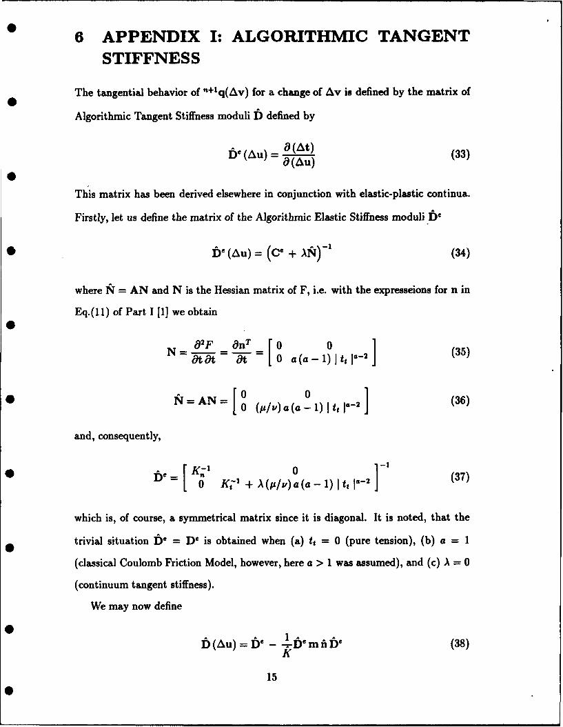
6 APPENDIX I: ALGORITHMIC TANGENTSTIFFNESS
The tangential behavior of "+ 1q(Av) for a change of Av is defined by the matrix of
Algorithmic Tangent Stiffness moduli b defined by
b e (Au) - 8(At) (33)0(Au)
This matrix has been derived elsewhere in conjunction with elastic-plastic continua.
Firstly, let us define the matrix of the Algorithmic Elastic Stiffness moduli 1ie
De(Au) = (Ce + AM)' (34)
where N = AN and N is the Hessian matrix of F, i.e. with the expresseions for n in
Eq.(11) of Part 1 [1] we obtain
N 2F OnT [ 0 0]t a2(5N = O- = t 0 a(a- 1) It " 2 (5
AN 0 0 -
* N = AN= [0 (pv) a(a - 1)ItI - ] (36)
and, consequently,
[ K-' + A (p/v)a(a- 1) it I-] (37)
which is, of course, a symmetrical matrix since it is diagonal. It is noted, that the
trivial situation b e = D e is obtained when (a) tt = 0 (pure tension), (b) a - 1
(classical Coulomb Friction Model, however, here a > 1 was assumed), and (c) A = 0
(continuum tangent stiffness).
We may now define
I) (Au)= f. - f(38)K
15
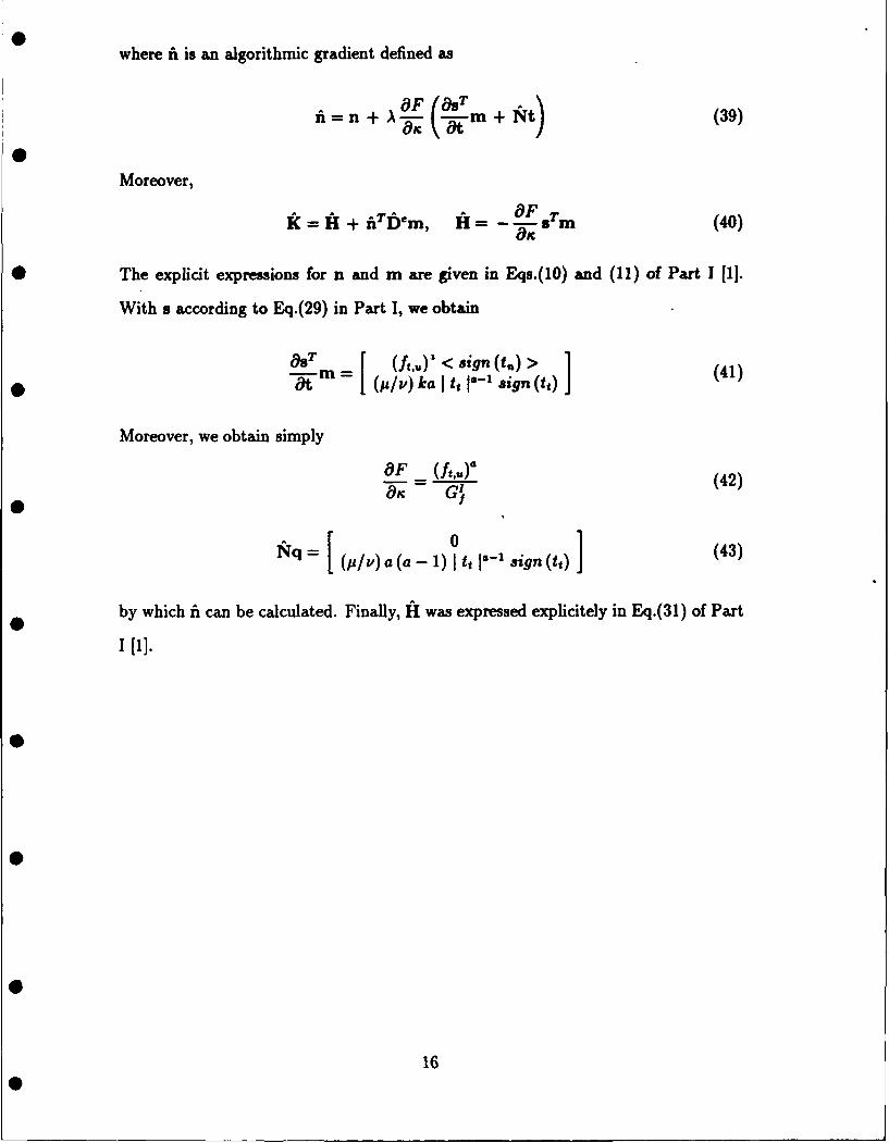
where fi is an algorithmic gradient defined as
n+A ( m + fqt) (39)
Moreover,
+ j)M j OF _T M (40)OFCIk= II+ fTIbm, H:I=- -sm40
The explicit expressions for n and m are given in Eqs.(10) and (11) of Part 1 [1].
With s according to Eq.(29) in Part I, we obtain
-- m (f,.)* < sign(t.) > (41)WM ~(p/v) ka I t, Ia-' sign (t,)
Moreover, we obtain simply
OF = (f,) (42)
[q 0i (43)
p = (pi~a (a- 1) I1f, sign (t,)
by which fi can be calculated. Finally, A was expressed explicitely in Eq.(31) of Part
I il].
0
0
16
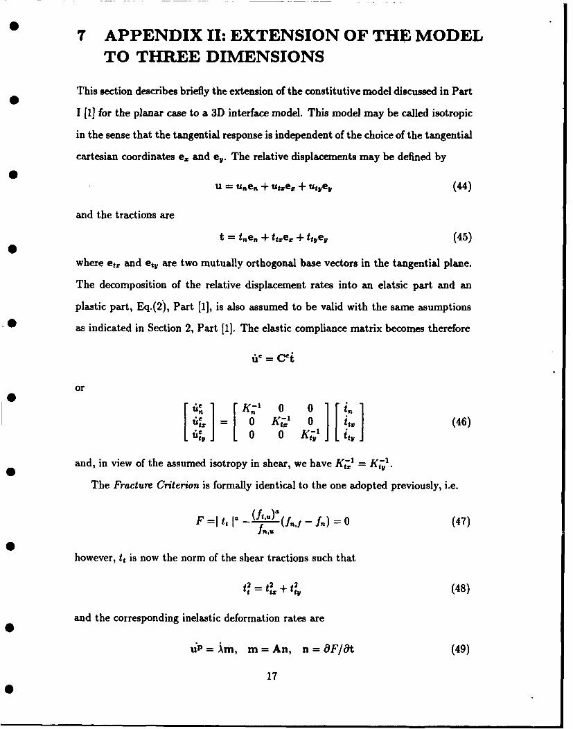
7 APPENDIX II: EXTENSION OF THE MODELTO THREE DIMENSIONS
This section describes briefly the extension of the constitutive model discussed in Part01 [1] for the planar case to a 3D interface model. This model may be called isotropic
in the sense that the tangential response is independent of the choice of the tangential
cartesian coordinates e, and ep. The relative displacements may be defined by
u = u~e, + ut.e. + ute, (44)
and the tractions are
t = te, + tte, + tte, (45)
where et. and et, are two mutually orthogonal base vectors in the tangential plane.
The decomposition of the relative displacement rates into an elatsic part and an
plastic part, Eq.(2), Part [1], is also assumed to be valid with the same asumptions
as indicated in Section 2, Part [1]. The elastic compliance matrix becomes therefore
f, =Cei
or
10 ii 0 K;' 0 it. (46)
J 1 0 0 K-' ity
and, in view of the assumed isotropy in shear, we have K;-' K;'.
The Fracture Criterion is formally identical to the one adopted previously, i.e.
F = t I a (ft")(fn - fA) = 0 (47)
however, tj is now the norm of the shear tractions such that
t2 = t2 + t2 (48)
and the corresponding inelastic deformation rates are
uP= m, m=An, n=OF/0t (49)
17

and
1 0 0]
A= 0 /V Oj , n= a (t, + t 2)(f 1) t I sign(tt=) (50)0 0 aply 2 (I 't+ t t - ) ta I sign(t,,)
The generalization of the work-softening hypothesis to three dimensions is incorpo-
rated in the new definition of the tangential shear tractions and the tangential inelastic
deformation. The rate law for the fracture energy release ic is again formally identical
with Eq.(18),
k =< t,, > tiP + k(tt - ft,,,)f (51)
however, tfi is now defined by
(fp)2 = (lp)2 + (52)
and tt and ft,, have been defined in Eq.(48) and Eq.(19), Part I,[1] respectively.
8 APPENDIX III: REFERENCES
Ottosen, N., Runesson, K. (1989)," Properties in Bifurcation Solution in Elasto-Plasticity",
accepted for Publication in Int. J. Solids and Structures
Runesson, K., Sure, S. and Willam, K.J. (1988)," Integration in Computational Plas-
ticity", Computers and Structures, 30, pp. 119-130
Sobh, N. (1987),"Bifurcation Analysis of Tangential Operators", Ph.D. Thesis Dept.
CEAE, University of Colorado, Boulder, Colorado
Stankowski, T. (1990),"Numerical Simulation of Progressive Failure in Particle Com-
posites",Ph.D. Thesis Dept. CEAE, University of Colorado, Boulder, Colorado
Stankowski, T., Runesson, R. and Sture, S. (1991),"Fracture and Slip of Interfaces in
Cementitious Composites", ASCE J. Eng. Mech., submitted for publication
Wiilam, K. J., Bicanic, N., Pramono, E. and Sture, S.,"Composite Fracture Model
for Strain Softening Computations of Concrete", Fracture Mechanics of Concrete -
Fundamentals and Applications, Ed. Wittman, 1, pp. 221-235
18

09 APPENDIX IV: NOTATION
C = compliance
D = stiffness
f = strength values
F = fracture function
m = gradient of plastic potential
n = gradient of fracture function
r = contact nodal forces
t = vector of contact traction
u = vector of relative displacements
p = vector of nodal displacements
x = eigenvectors
a = coefficient
# = coefficient
A = plastic multiplier
* = measure of released fracture energy
U = finite element shape functions
o = stresses
= strains
Superscripts
() = rate, differentiation with respect to (pseudo) time
e = elastic
p = plastic
Subscripts
n = normal direction
19

r = residual values
t = tangential direction
u = ultimate (peak) values
20
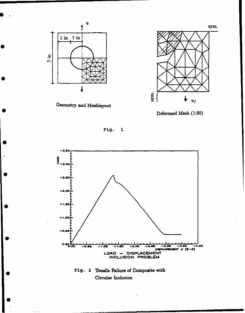
U
sym.
Geometry and Meshlayout U
Deformed Mesh (1:50)
Fig. 1
0
-2.5O0
-2.00
0.0 -06 -1.00 -1.60 -2.00 -2.60 -3.00 -3.60 -.4.00captL'cadD4 U [IC-33
LOAD - DISPLACEMENTINCLUSION PROBLEM
Fig. 2 Tensile Failure of Composite with
Circular Inclusion

PART 3 INTERFACE EXPERIMENTS
1. INTRODUCTION
Interface experiments were conducted to investigate the modeof debonding, de-cohesion, fracture and slip of the mortar-aggregate composite, and an experimental apparatus was manu-factured to achieve these objectives. The apparatus is cap-able of loading the interface specimens in combined tension-shear or compression shear modes, and it is sufficientlystiff to maintain overall specimen-loading apparatus stab-ility throughout the debonding, fracture, and slip process.
This section describes experimental technique, apparatus,and results. A total of 52 experiments were conducted ofwhich 32 were successful.
2. APPARATUS
The combined tension-shear and compression-shear interfaceexperimental apparatus consists of two components, in that ageneral purpose MTS (Minnesota Testing Systems) 490 kN (110kips) universal servo-controlled loading frame, that wasoperated in displacement control, is used as the externalloading agency and provides the normal load to the inter-faces in the smaller tangential interface loading apparatus,which is also operated in displacement control by means of astiff constant speed screw-actuator. The apparatus isfurnished with several linear variable differential trans-formers (LVDTs), which records absolute and relative tang-ential and vertical (normal) displacements in the matrix(mortar)-aggregate (granite) interface specimens. Loadcells in the MTS and interface apparatus were used to recordglobal loads or reactions. The interface apparatus is rela-tively compact and structurally stiff, and fits between thereaction frame of the MTS testing machine as seen in Figs. 1and 2. Figures 3 and 4 show the LVDT placements, whichshow the measurement gage-points close to the interfaceitself.
The apparatus has a normal load capacity of nearly 50 kN incompression or tension (normal load over the interface), anda shear load capacity of also 50 kN. the resolution andaccuracy of the system is relatively high, and loads assmall as 0.05 N can be recorded. The precision gageheads(LVDTs) can measure displacements as small as 0.01 mm, withan accuracy of 0.005 mm. Since the stiffness of the appa-ratus is finite the relative displacements of the interfacein both the tangential and normal directions are recorded aswell as the total displacement measurement. This ensuresaccurate control and recording of the various motions. Inmost of the experiments described in the following the max.
1
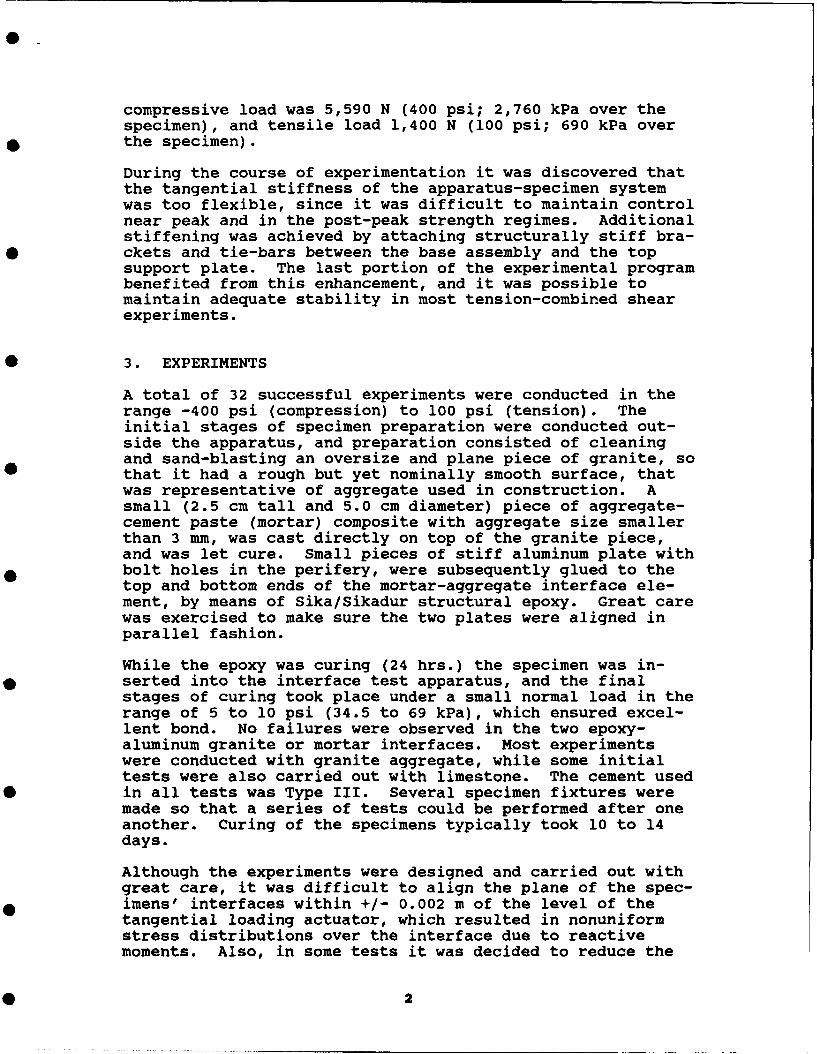
compressive load was 5,590 N (400 psi; 2,760 kPa over thespecimen), and tensile load 1,400 N (100 psi; 690 kPa overthe specimen).
During the course of experimentation it was discovered thatthe tangential stiffness of the apparatus-specimen systemwas too flexible, since it was difficult to maintain controlnear peak and in the post-peak strength regimes. Additionalstiffening was achieved by attaching structurally stiff bra-ckets and tie-bars between the base assembly and the topsupport plate. The last portion of the experimental programbenefited from this enhancement, and it was possible tomaintain adequate stability in most tension-combined shearexperiments.
3. EXPERIMENTS
A total of 32 successful experiments were conducted in therange -400 psi (compression) to 100 psi (tension). Theinitial stages of specimen preparation were conducted out-side the apparatus, and preparation consisted of cleaningand sand-blasting an oversize and plane piece of granite, sothat it had a rough but yet nominally smooth surface, thatwas representative of aggregate used in construction. Asmall (2.5 cm tall and 5.0 cm diameter) piece of aggregate-cement paste (mortar) composite with aggregate size smallerthan 3 mm, was cast directly on top of the granite piece,and was let cure. Small pieces of stiff aluminum plate withbolt holes in the perifery, were subsequently glued to thetop and bottom ends of the mortar-aggregate interface ele-ment, by means of Sika/Sikadur structural epoxy. Great carewas exercised to make sure the two plates were aligned inparallel fashion.
While the epoxy was curing (24 hrs.) the specimen was in-serted into the interface test apparatus, and the finalstages of curing took place under a small normal load in therange of 5 to 10 psi (34.5 to 69 kPa), which ensured excel-lent bond. No failures were observed in the two epoxy-aluminum granite or mortar interfaces. Most experimentswere conducted with granite aggregate, while some initialtests were also carried out with limestone. The cement usedin all tests was Type III. Several specimen fixtures weremade so that a series of tests could be performed after oneanother. Curing of the specimens typically took 10 to 14days.
Although the experiments were designed and carried out withgreat care, it was difficult to align the plane of the spec-imens' interfaces within +/- 0.002 m of the level of thetangential loading actuator, which resulted in nonuniformstress distributions over the interface due to reactivemoments. Also, in some tests it was decided to reduce the
2

area of the interface by reducing the diameter of the mortarphase's contact diameter by 0.75 cm. This helped stabilizethe low normal (confin-ing) stress experiments.
Nonlinear finite element analyses of the specimen-apparatussystem were also conducted to help analyze and characterizethe interface properties. These analyses have been desc-ribed earlier by Stankowski (1990 a and b) and Stankowski etal. (1990 and 1991). It was established that the nominal oraverage properties for the interfaces were quite close towhat was developed during the course of the numerical ana-lysis-and-experiment inverse identification studies. Thelast figure in this report (Fig. 21) clearly shows that theinterface properties (curved ultimate strength envelope,residual strength envelope, and various constants) match thedata closely.
4. EXPERIMENTAL DATA
Figures 6 (a) - (e) through 20 (d) - (f) show load-displace-ment response diagrams for typical successful experimentsconducted in the range -400 psi (-2,760 kPa) compressivenormal stress to 100 psi (690 kPa) tensile normal stress.The diagrams (a) through (e) in each case show: (a) shearstress vs. normal displacement; (b) shear stress vs. shear(horizontal) displacement (total); (c) shear stress vs.shear (horizontal) displace-ment (bottom relative gage pointlocation); (d) shear stress vs. shear (horizontal) dis-placement (top relative gage point location); and, (e)normal displacement vs. shear (horizontal) displacement,which is an indication of dilatancy of the interface duringshearing. The "noise" seen in many of the response diagramsare due to characteristics of the signal processing and dataacquisition units, and it is not connected to the nature ofthe experiments themselves. Further smoothing of the datawill be conducted in subsequent paper preparation efforts.
It is noted that the experiments conducted at higher stresslevels remained stable for longer periods than the low nor-mal stress tests, which at times became quite unstable. Therate of dilatancy of the interfaces increases with lowernormal stress ranges, and tends to diminish with higherstresses that suppress dilatancy. In the tensile loadingcases where global instabilities often followed peak stren-gth, it seems that the post-peak slopes for stable pathswere an order of magnitude steeper that the ones observed.When comparing the experimental data with model performance,it seems that the model simulates behavior at all normalstress levels quite well. Also the normal displacement(dilatancy) response appears quite realistic. Peak andresidual strength data for all tests are presented in Fig.21. The open "squares" represent peak strength information,
0 3

and the "crosses" represent residual strength data. Themodel parameters that were obtained from this informationare also shown in the figure.
(Please not that the following pages with figures anddiagrams have not been paginated)
4
0 R
LIST OF FIGURES
Fig. 1 Combined tension-shear or compression-shearmortar-aggregate experimental apparatus
Fig. 2 (a) Apparatus mounted in MTS (490 kN) servo-controlled load frame. (b) Experimentalapparatus with tangential displacementcontrolled screw-actuator.
(a) (b)
Fig. 3 (a) and (b) Experimental apparatus withLVDTs used for measurement of relativetangential and normal displacements
(a) (b)
Fig. 4 (a) Experimental apparatus with relativemotion displacement transducers and mortar-aggregate interface specimen. (b) Mortar-aggregate (granite) specimen with attachedaluminum base plates
(a) (b)
Fig. 5 (a) Top view, and (b) side view of mortar-aggregate (granite) specimen with bottomaluminum base plate
(a) (b)
Fig. 6 (a) - (e) Load-displacement response diagramsfor test series 1
Fig. 7 (a) - (e) Load-displacement response diagramsfor test series 7
Fig. 8 (a) - (e) Load-displacement response diagramsfor test series 11
Fig. 9 (a) - (e) Load-displacement response diagramsfor test series 12
Fig. 10 (a) - (e) Load-displacement response diagramsfor test series 13
Fig. 11 (a) - (e) Load-displacement response diagramsfor test series 14
Fig. 12 (a) - (e) Load-displacement response diagramsfor test series 15
5
Fig. 13 (a) - (e) Load-displacement response diagramsfor test series 21
Fig. 14 (a) - (e) Load-displacement response diagramsfor test series 22
Fig. 15 (a) - (f) Load-displacement response diagramsfor test series 23
Fig. 16 (a) - (e) Load-displacement response diagramsfor test series 24
Fig. 17 (a) - (f) Load-displacement response diagramsfor test series 28
Fig. 18 (a) - (f) Load-displacement response diagramsfor test series 29
Fig. 19 (a) - (f) Load-displacement response diagramsfor test series 30
Fig. 20 (a) - (f) Load-displacement response diagramsfor test series 31
Fig. 21 Ultimate (Peak) and residual strength envelopes formortar-aggregate (granite) interfaces and cali-brated model parameters
6

* [El MOVING X-HEAD n] LOAD CELL j
TEE BAR
SLEDGE SYSTEM
S ACTUATOR
/////////777///
• Fig. 1 Combined tension-shear or compression-shearmortar-aggregate experimental apparatus

0
(a)
0I
. ,
(b)
Fig. 2 (a) Apparatus mounted in MTS (490 kN) servo-controlled load frame. (b) Experimentalapparatus with tangential displacementcontrolled screw-actuator.

(a)
(b)
Fig. 3 (a) and (b) Experimental apparatus withLVDTs used for measurement of relativetangential and normal displacements
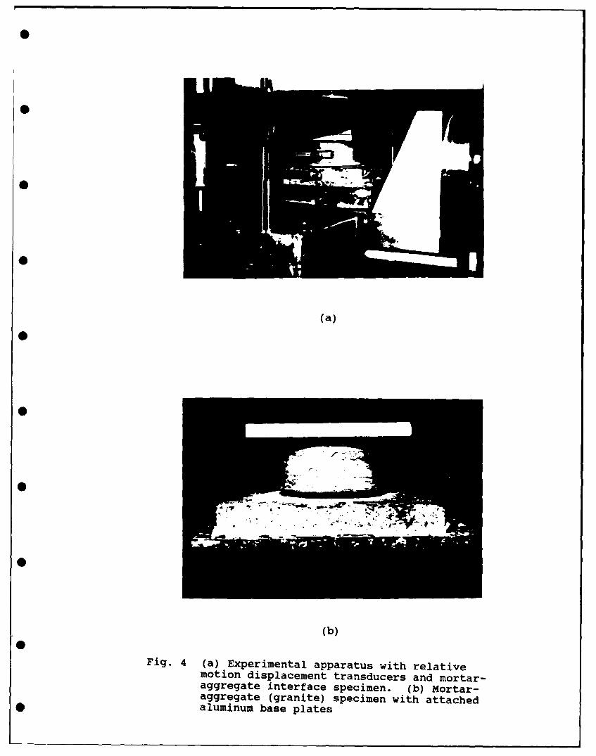
0L
(a)
0
(b)
Fig. 4 (a) Experimental apparatus with relativemotion displacement transducers and mortar-aggregate interface specimen. (b) Mortar-aggregate (granite) specimen with attached• aluminum base plates

0~0
(a)
(b)
Fig. 5 (a) Top view, and (b) side view of mortar-aggregate (granite) specimen with bottomaluminum base plate

Normal Displacement -Shear Stress600Normal Stress =-100 psi. Htestla
500-
400-j
~300-
1/)
0
0 0.02 0.04Normal Displacement (in)
Fig.- (a) -(e) Load-displacement response diagramsfor test series 1
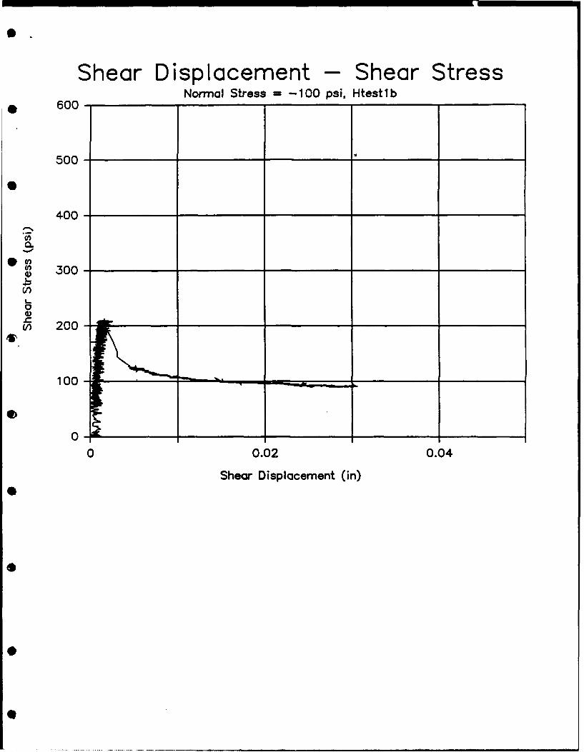
Shear Displacement -Shear Stress600-Normal Stress =-100 psi, Htestlb
500-
400-
ft0.
S300-
V)
0 0.02 0.04
0 Shear Displacement (in)
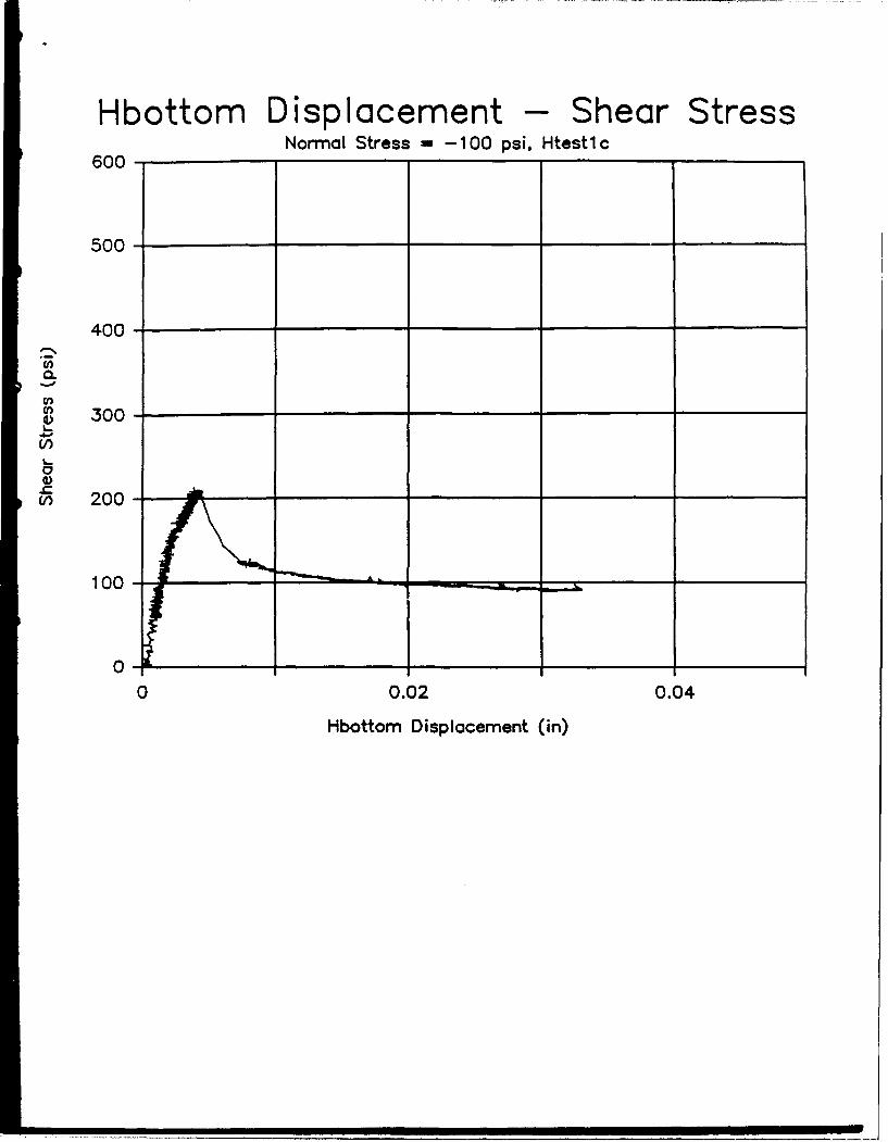
Hbottom Displacement -Shear Stress600-Normal Stress =-100 psi, Htestl c
600-
500-
400-
En
2 00-
1, 00-
0-0 0.02 0.04
Hbottom Displacement (in)
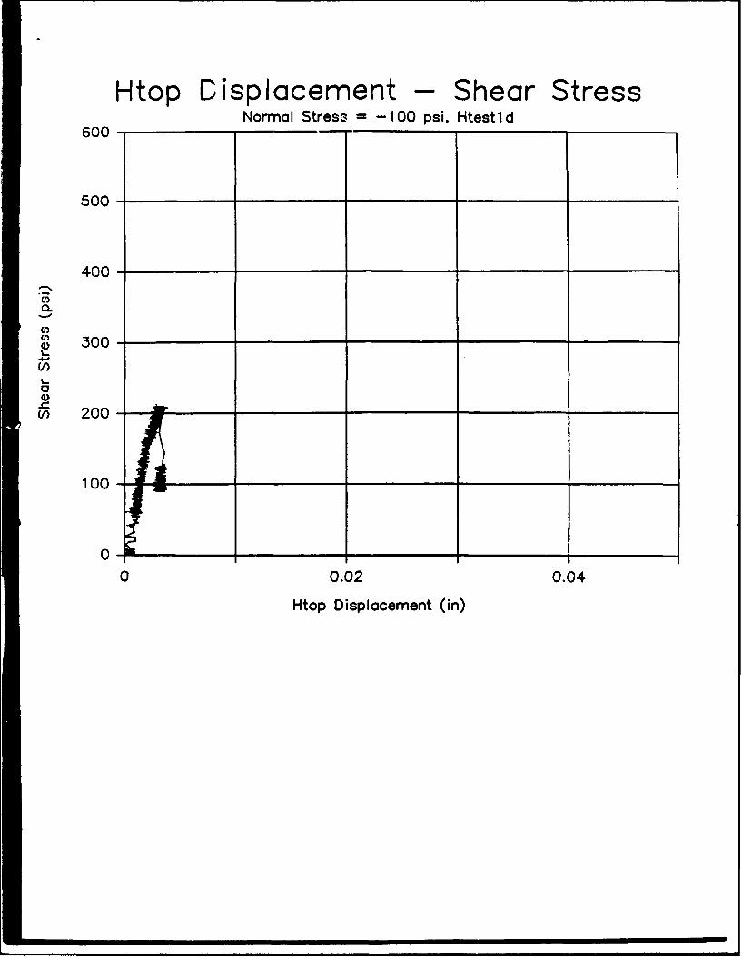
Htop Displacement - Shear StressNormal Stress -100 psi, Htestl d
600-
500-
400-
U)
G) 300~U-)
v 200-
100-
0-0 0.02 0.04
Htop Displacement (in)
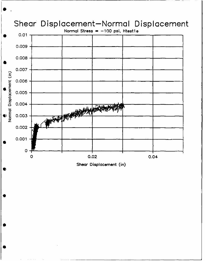
Shear' Displacement-Normal DisplacementNormal Stress =-100 psi, Htestle
* 0.01 -
0.009-
0.008 - _ _ _ _ _ _ _ _ _ _ _ _ _ _ _ _ _ _ _ _
0.007 - _ _ _ _ _ _ _ _ _ _ _ _ _ _ _ _ _ _ _
C 0.006-
0.05
0z
.00000
00
00.200
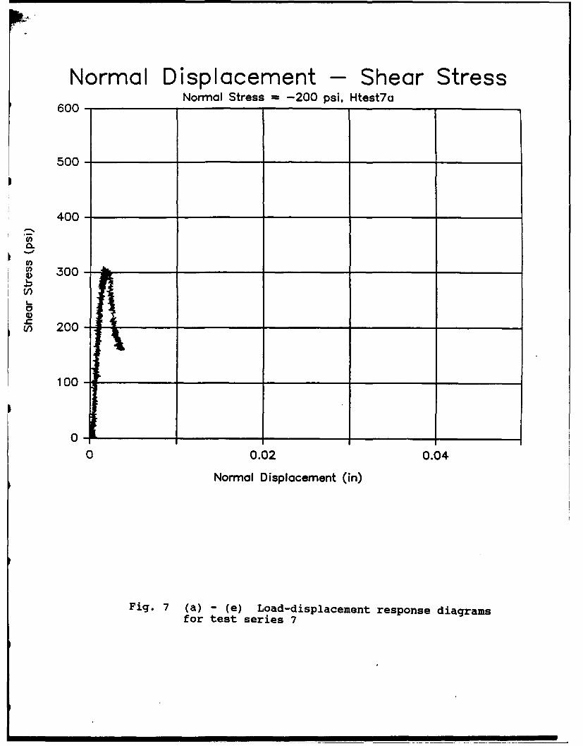
Normal Displacement - Shear StressNormal Stress -200 psi, Htest7a
600-
500-
400-
Co
4)
0
0 0.02 0.04
Normal Displacement (in)
Fig. 7 (a) - (e) Load-displacement response diagramsfor test series 7
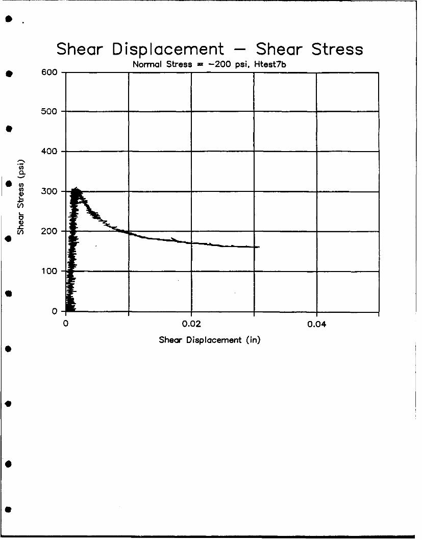
Shear Displacement - Shear StressNormal Stress =-200 psi, Htest7b
* 600-
500-
400-
Co
En
~, 300-*VI)
V) 20
100-
00
0 0.02 0.04
Shear Displacement (in)
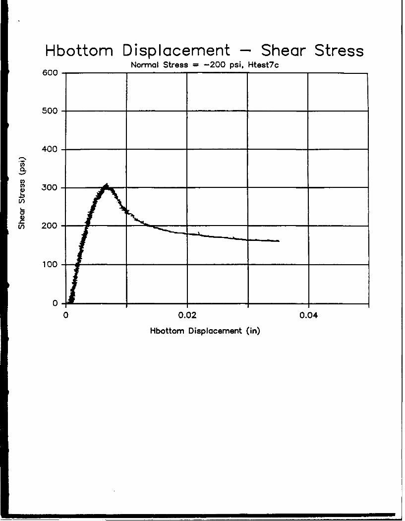
Hbottom Displacement -Shear StressNormal Stress =-200 psi. Htest7c
600-
500-
400-
200
0-1
0 0.02 0.04
Hbottom Displacement (in)
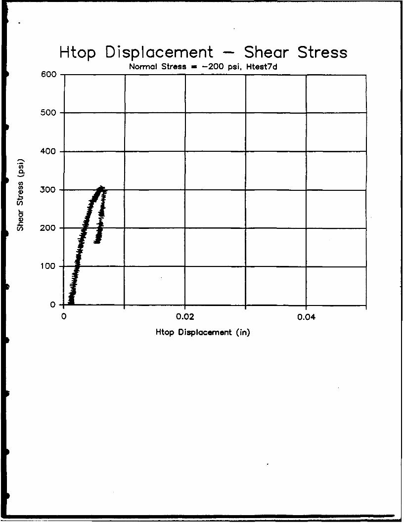
Htop Displacement - Shear Stress0 600-Normal Stress -- 200 psi. Htest7d
500-
500-
S300-t/)
S200-
10-
0 0.02 0.04
Htop Displacement (in)
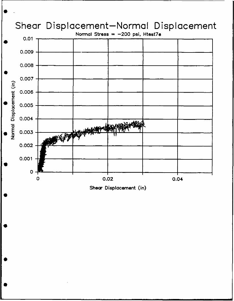
Shear Displacement-Normal D isp lacementNormal Stress -200 psi, Htest7e
0 0.01 -
0.009 - _ _ _ _ _ _ _ _ _ _ _ _ _
0.008 - _ _ _ _ _ _ _ _ _ _
0.07
C
S0.006 - ____
S0.004 - _ _ _ _ _ _ _ _ _ _ _ _ _ _ _ _ _ _ _ _
E0.003-
0.002 - F_ _ _ _ _ _ _ _ _ _
0 0.02 0.04
Shear Displacement (in)
40
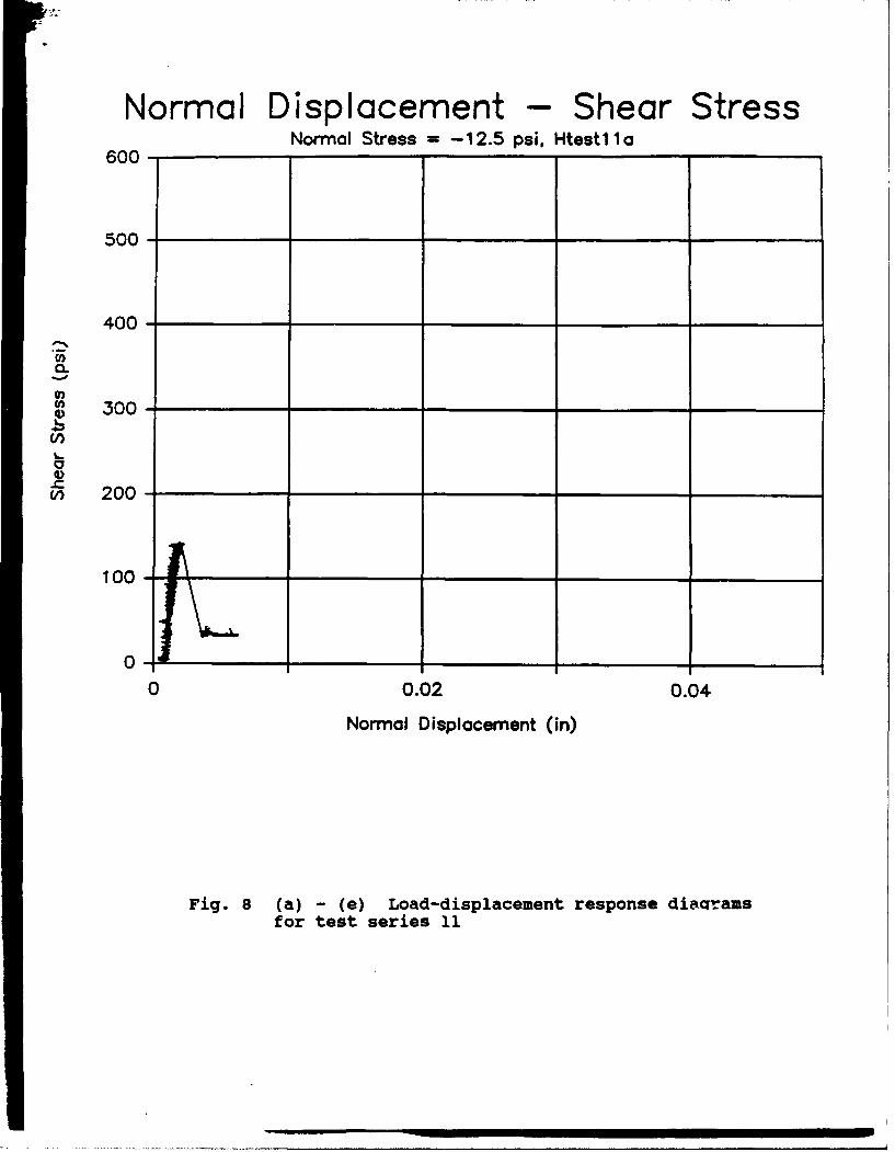
Normal Displacement - Shear StressNormal Stress =-12.5 psi. Htestl 10
600-
500-
400-
0~
0 0.000.0
Noml ipacmnt(n
Fi.8 () () La-ipaeetrsos i0-asfo0etseis1

Shear Displacement - Shear StressNormal Stress = 12.5 psi. Htestl l b
600-
500-
400-
0.0
100300
0-10 0.02 0.04
Shear Displacement (in)
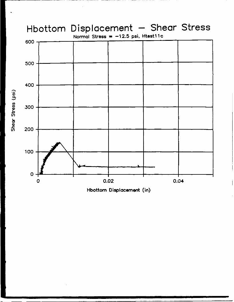
Hbottom Displacement -Shear StressNormal Stress = 12.5 psi. Htestl 11 c
600-
5o0-
400-
0.0
En
2 00-
100 -
0-----
0 0.02 0.04
Hbottom Displacement (in)
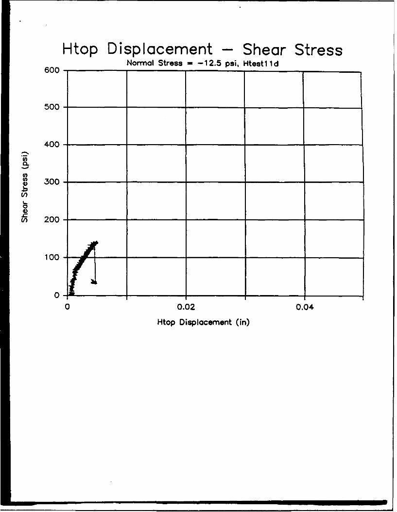
Htop Displacement -Shear StressNormal Stress - 12.5 psi, Htestl 11 d
600-
500-
400-
300-C,)
v, 200-
100-
0-0 0.02 0.04
Htop Displocemnent, (in)
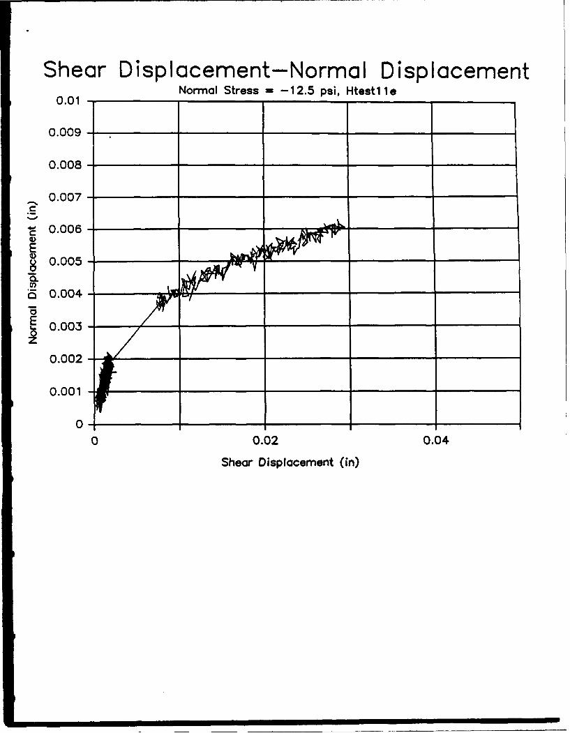
Shear Displacement-Normal Displacement0.01 -Normal Stress = 12.5 psi, Htestl 11e
0.019-
0.008 - _ _ _ _ _ _ _ _ _ _ _ _ _ _ _
_ 0.007 - _ _ _ _
C 0.006 - _ ____
q)E
0.005 - __ _ _ _ _ _ _ _ _ _
C)
0 0.02 0.04
Shear Displacement (in)

Normal Displacement - Shear StressNormal Stress =-12.5 psi, Htestl2o
600-
500-
400-
a.
S 300-C,)
(/) 200-
100-- _ _ _ _
0-10 0.02 0.04
Normal Displacement (in)
Fig. 9 (a) -(e) Load-displacement response diagramsfor test series 12
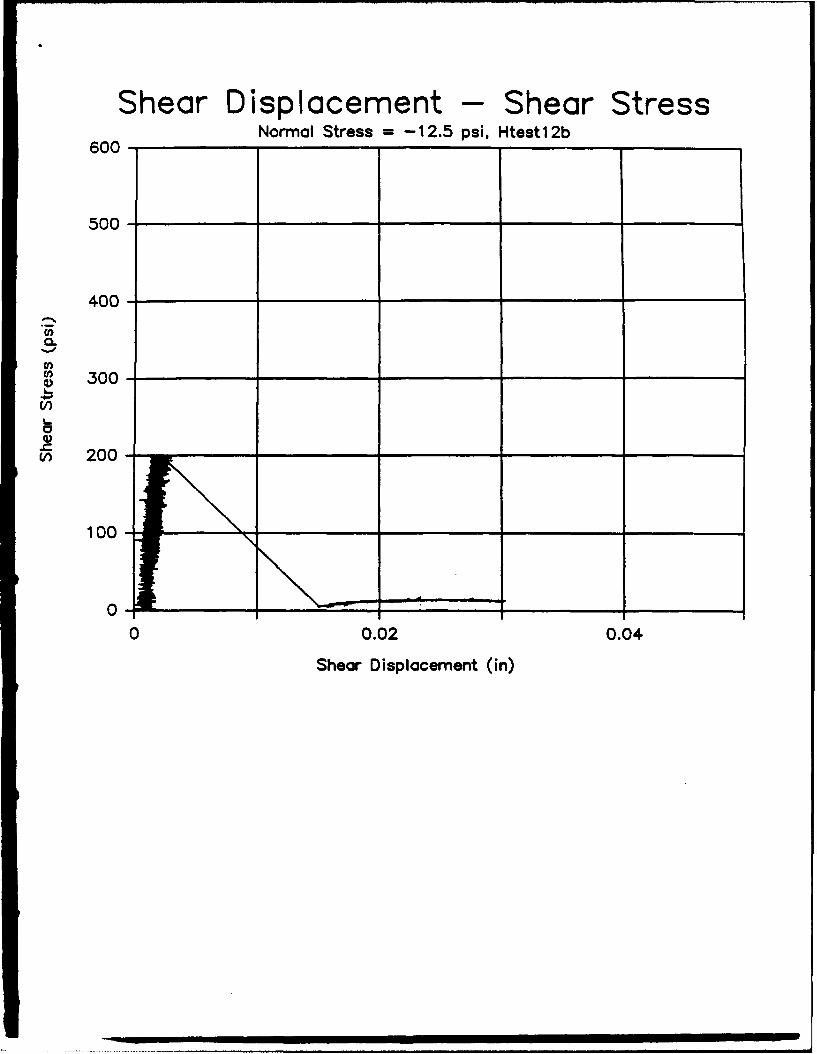
Shear Displacement -Shear StressNormal Stress = 12.5 psi, Htest 1 2b
600-
500-
400-
0.
CO 300-(I)
00
0 0.02 0.04
Sheaor Displacement (in)
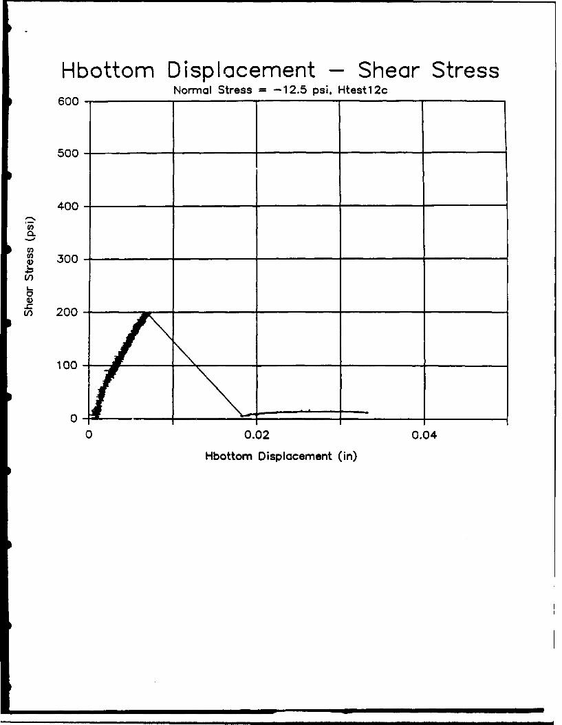
Hbottomn Displacement - Shear Stress600-Normal Stress =-12.5 psi, Htestl2c
500-
400-
100
00100 0.02_____ 0.04__________________
Hbttr 300-ceen (n

Htop Displacement - Shear StressNormal Stress = 12.5 psi, Htestl1 2d
600- ____
500-
400-
U)
-90
0,
V) 300-
10-
00
0 0.02 0.04
Htop Displacement (in)
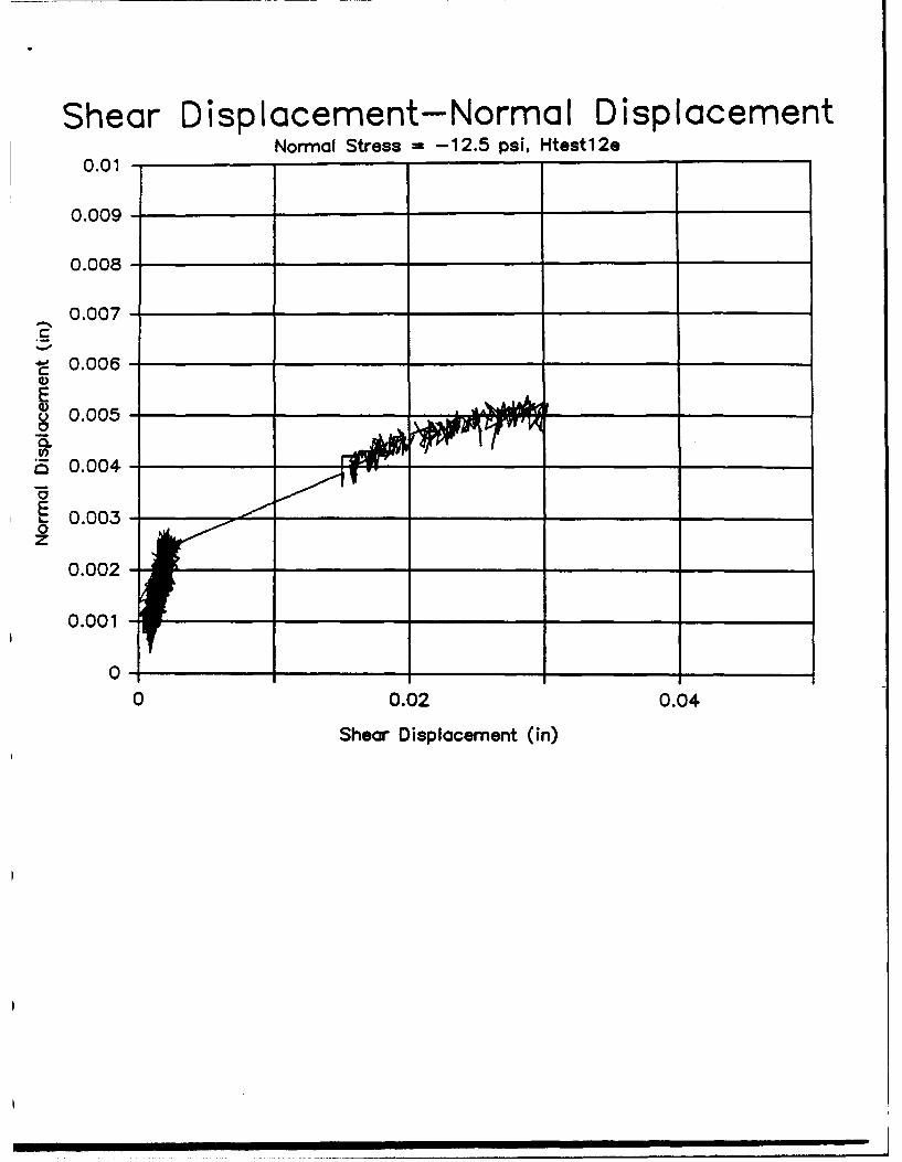
Shear Displacement-Normal DisplacementNormal Stress =-12.5 psi, Htestl2e
0.01 - _ _ _ _ _
0.009 - _ _ _ _ _ _ _ _ _ _ _ _ _ _ _
0.008 - _ _ _ _ _ _ _ _ _ _ _ _ _ _ _ _ _ _ _ _ _ _ _ _ _
0.007 - _ _ _ _ _ _ _ _ _ _ _ _ _ _ _ __ _ _ _
40' 0.006 - _____ _____ _____ _____
C
E
0.05
6 0.004 - _ _ _ _ _ _ _ _ _ _ _ _ _ _
0z
0 0.02 0.04
Shear Displacement (in)
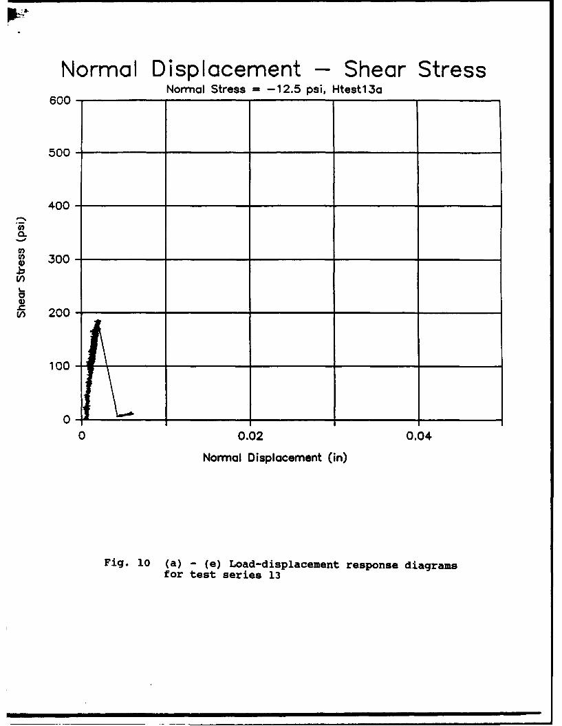
Normal Displacement - Shear StressNormal Stress =-12.5 psi, Htestl3a
600-
500-
400-
300
(I)
V) 200-
100 -
0-1110 0.02 0.04
Normal Displacement (in)
Fig. 10 (a) -(e) Load-displacement response diagramsfor test series 13

Shear Displacement - Shear StressNormal Stress =-12.5 psi, Htestl 3b
600-
500-
400-fz
CO300-
(I)
V) 200-
100 -
0-1_ _ _ _ ~_ _ _ _
0 0.02 0.04
Shear Displacement (in)
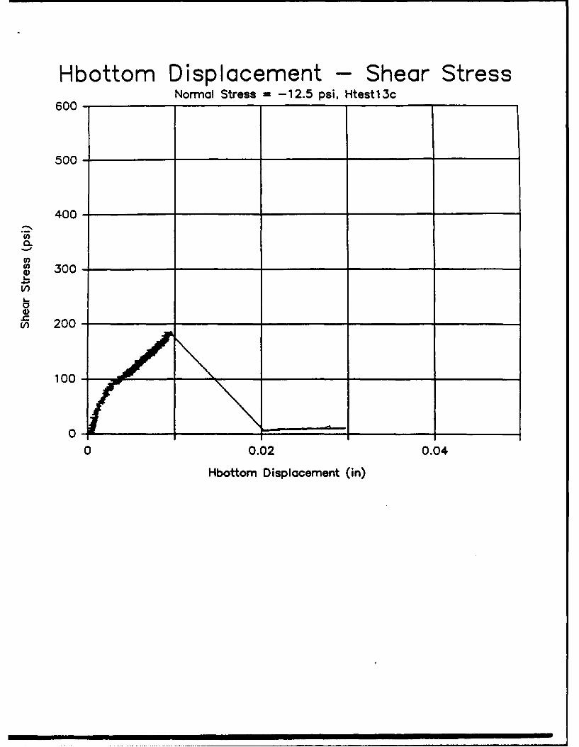
Hbottomn Displacement - Shear StressNormal Stress =-12.5 psi, Htestl3c
600-
500-
400-
C',
0 300-V)
Vn 200-
100 - _ _ _ _ _ _ _ _
0-10 0.02 0.04
Hbottomn Displacement (in)
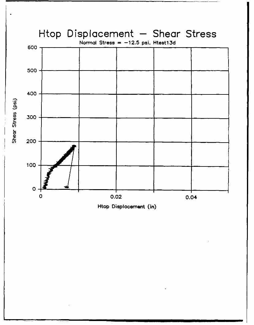
Htop Displacement - Shear Stress600-Normal Stress -- 12.5 psi. Htestl3d
500-
400-
a.
S300-
V)
V) 200-
100 -
0-0 0.02 0.04
Htop Displacement (in)
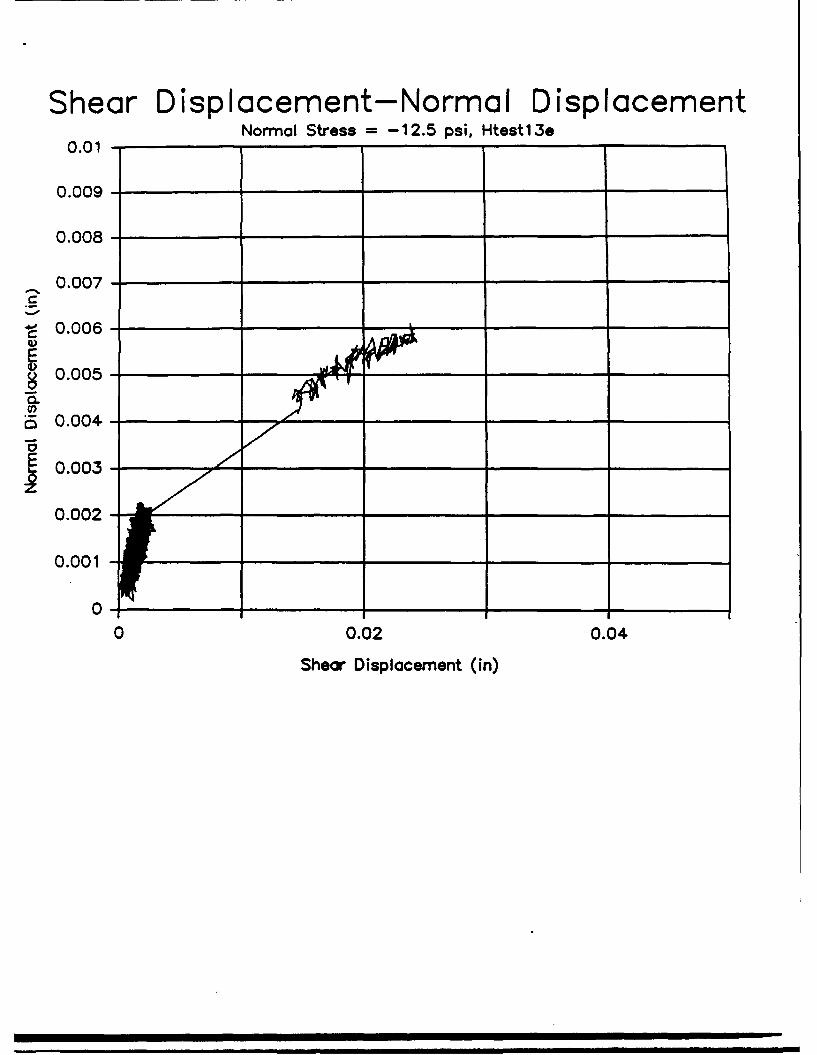
Shear Displacement-Normal DisplacementNormal Stress = 12.5 psi, Htestl1 3.
0.01 - _ _ _ _ _ _ _ _ _ _ _ _ _ _ _ _ _ _ _ _ _ _ _ _ _ _
0.009 - _ _ _ _ _ _ _ _ _ _
0.008 - _ _ _ _ __ _ _ _ _ _ _ _ _ _ _ _ _ _ _
_0.007-
S0.006 - _ _ _ _ _ _ _ _ _ _ _ _ _ _ _ _ _ _ _
0.005 - _ _ _ _ _ _ _ _ _ _
0.001 - _ _ _ _ _
0-0 0.02 0.04
Shear Displacement (in)
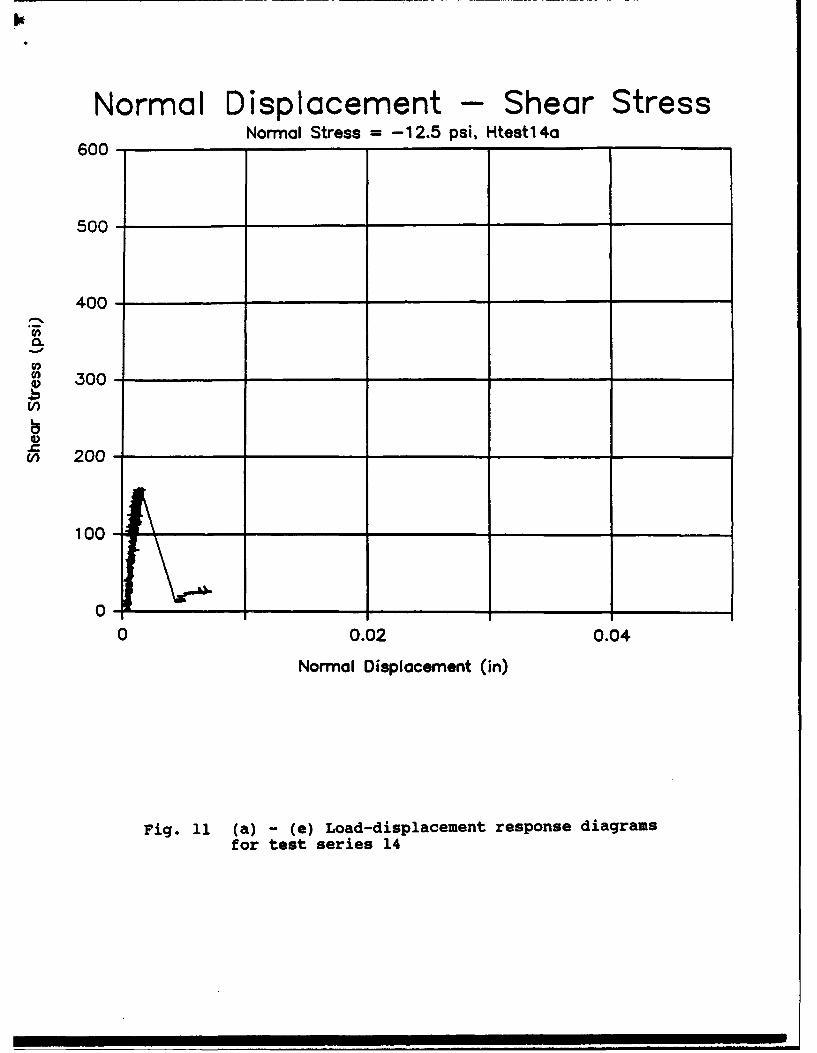
Normal Displacement - Shear StressNormal Stress =-12.5 psi, Htestl4a
600-
500-
400-
a.S.P
S300-
V)
V) 200-
100-
0-0 0.02 0.04
Normal Displacement (in)
Fig. 11 (a) -(e) Load-displacement response diagramsfor test series 14
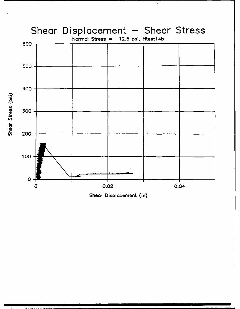
Shear Displacement - Shear StressNormal Stress =-12.5 psi, Htestl 4b
600-
500-
400-
%0
S300-
V)
S200-
100 -
0-10 0.02 0.04
Shear Displacement (in)
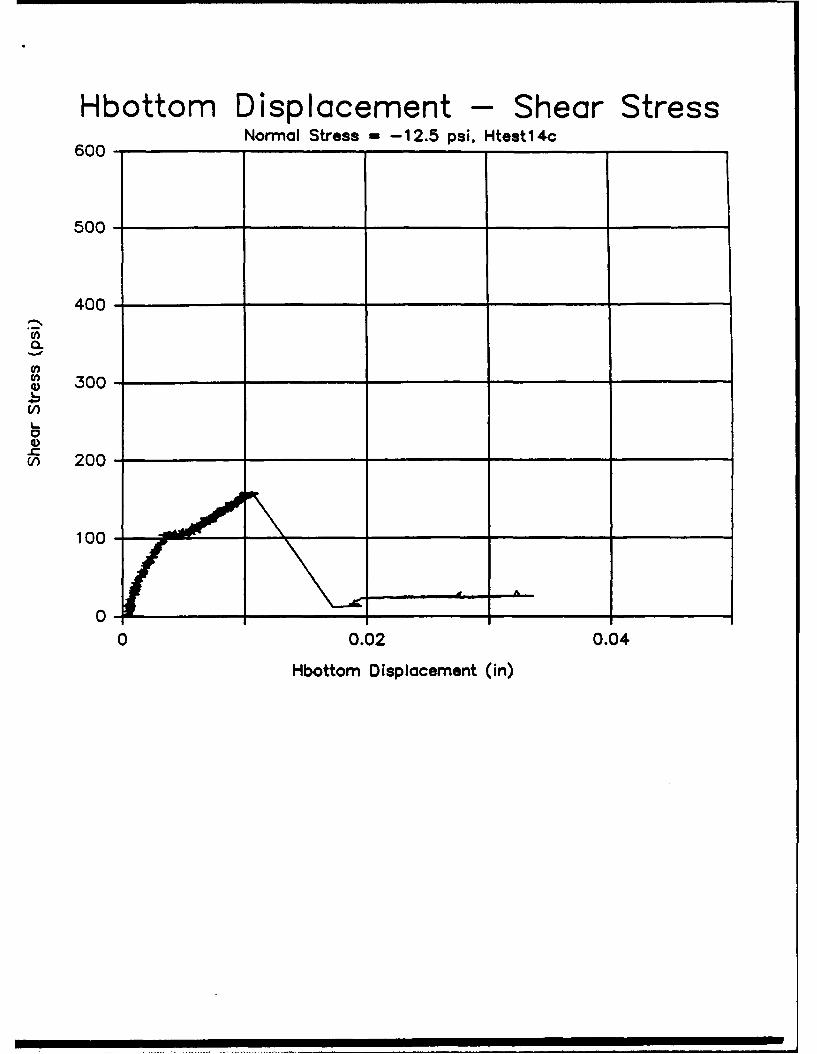
Hbottomn Displacement - Shear StressNormal Stress -- 12.5 psi, Htestl 4c
600-
500-
400-
C,
q~300-
C,)
1 00-
0 0.02 0.04
Hbottom Displacement (in)

Htop Displacement - Shear StressNormal Stress =-12.5 psi, Htestl4d
600-
500-
400-
300
-V
300--
00
0 0.02 0.04
Htop Displacement (in)
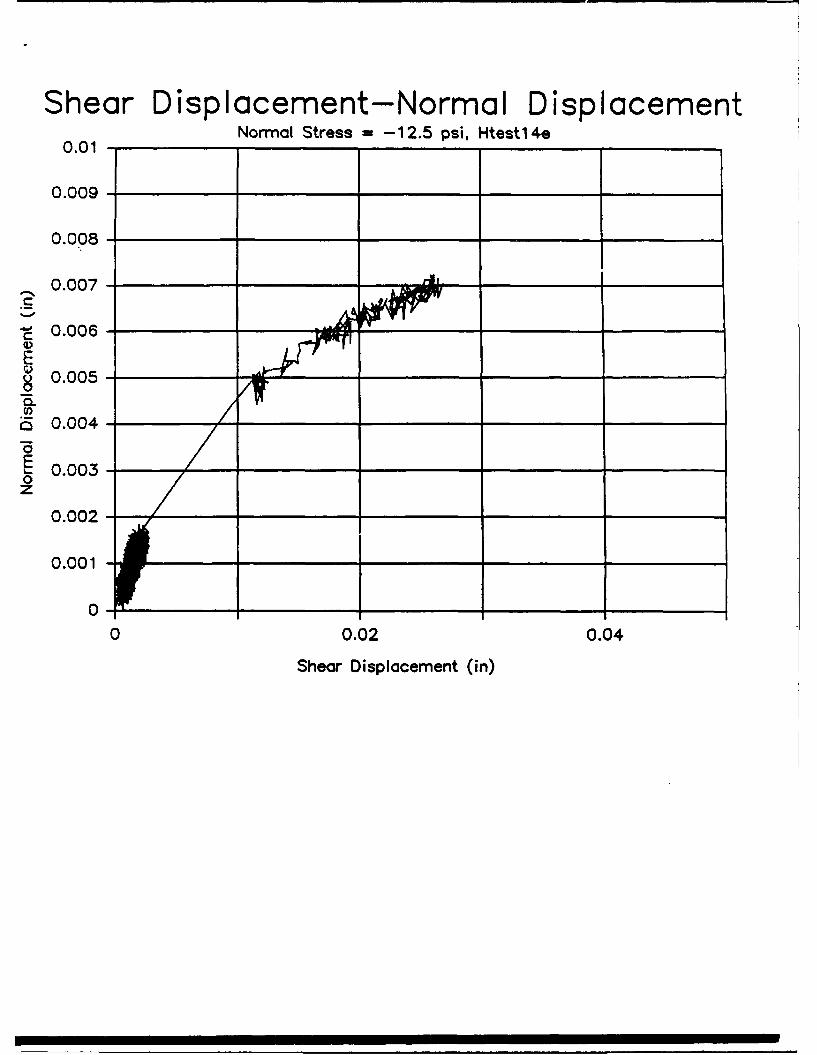
Shear Displacement-Normal DisplacementNormal Stress = 12.5 psi, Htestl 4.
0.01 - _ _ _ _ _ _ _ _ _ _ _ _ _ _ _
0.009 - _ _ _ _ _ _ _ _ _ _ _ _ _ _ _ _ _ _ _ _ _ _ _ _ _
0.008 - __ ___
0.007 - _ _ _ _
C
-C 0.006 - _ _ _ _ _ _ _ _ _ __ _ _ _
ES0.005 - _ ____
S0.004 - _ _ _ _ _ _ _ _ _ _
0
0 0.02 0.04
Shear Displacement (in)
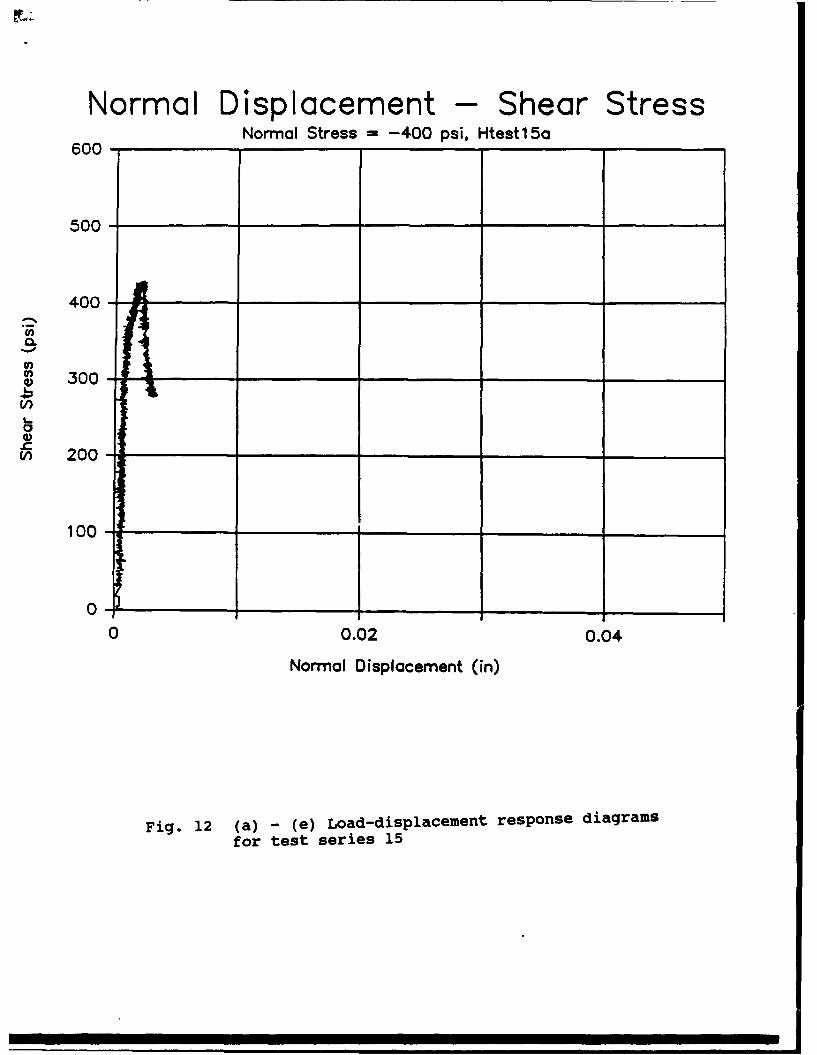
Normal Displacement - Shear StressNormal Stress =-400 psi, Htestl 5a
600-1
500-
400 -
0.
0 .0 00
0, ~ ~ ~ ~ ~ ~ ~ Nra Displacement_ (in)__________________
F00- 12 (a) _ _ _e)__ Loaddislacmen respnsediaram
fo ts sres1
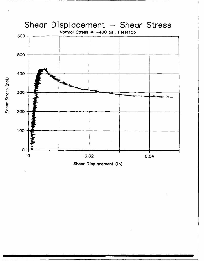
Shear Displacement Shear StressNormal Stress =-400 psi, Htestl 5b
600-
500-
400-
.200
1 00-
00
0 0.02 0.04
Shear Displacement (in)
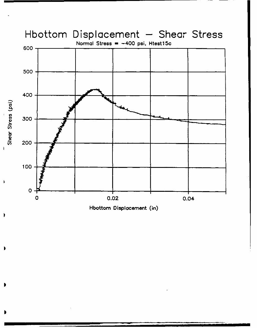
Hbottomn Displacement - Shearv StressNormal Stress =-400 psi. Htestl 5c
600-
500-
400-
0.0-.0 00
Hbto Dslcmet(n
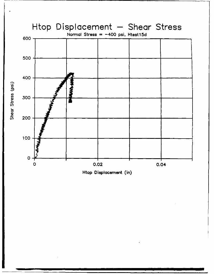
Htop Displacement - Shear StressNormal Stress =-400 psi. Htestl 5d
600-
500-
300-
0.00-.0 00
HtpDslceet(n
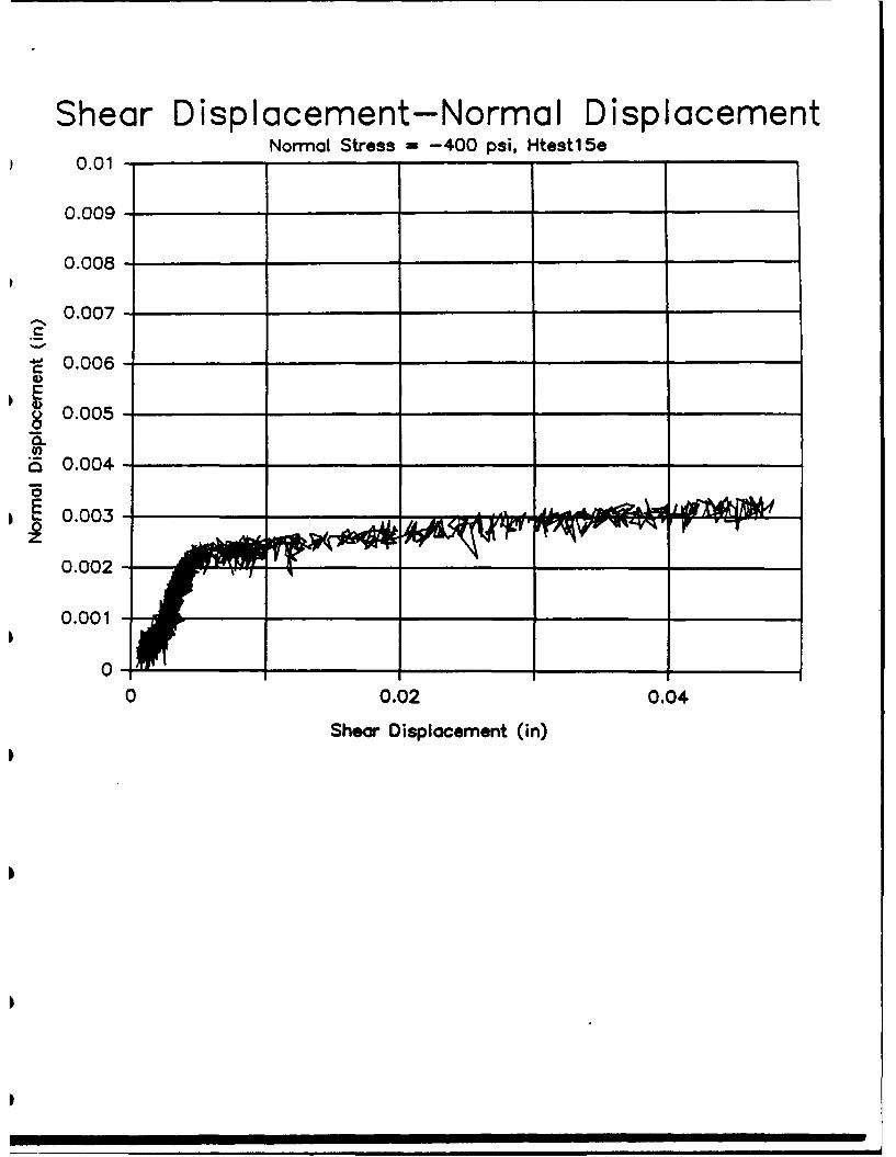
Shear Displacement-Normal DisplacementNormal Stress -- 400 psi, Htestl 5e
0.01 -
0.009 - _ _ _ _ _ _ _ _ _ _ _ _ _ _ _ _ _ _ _ _
0.008 - _ _ _ _
0.007 - _ _ _ _ _ _ _ _ _ _ _ _ _ _ _ _ _ _ _ _ _ _ _ _ _
C
t 0.006 - _ _ _ _ _ _ _ _ _ _ _ _ _ _ _ _ _ _ _ _ _ _ _ _
jS 0.004 - _ _ _ _ _ _ _ _ _ _ _ _ _ _ _ _ _ _ _ _
0.003-F
0.001 - _ _ _ _ _ _ _ _ _ _
0 0.02 0.04
Shear Displacement (in)
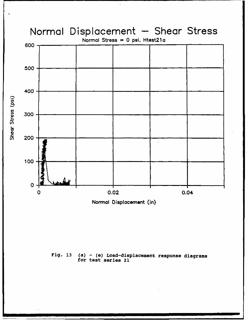
Normal Displacement - Shear StressNormal Stress = 0 psi, Htest2l a
600-
500-
400-
C,,0.
-300-V)
- 200- "100-
0
0 0.02 0.04
Normal Displacement (in)
Fig. 13 (a) - (e) Load-displacement response diagramsfor test series 21
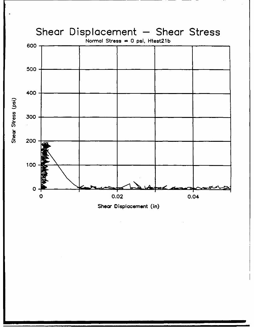
Shear Displacement - Shear StressNormal Stress 0 psi, Htest2lb
600-
500-
400-
S300-
LI)
S200-
100
0 0.02 0.04
Shear Displacement (in)
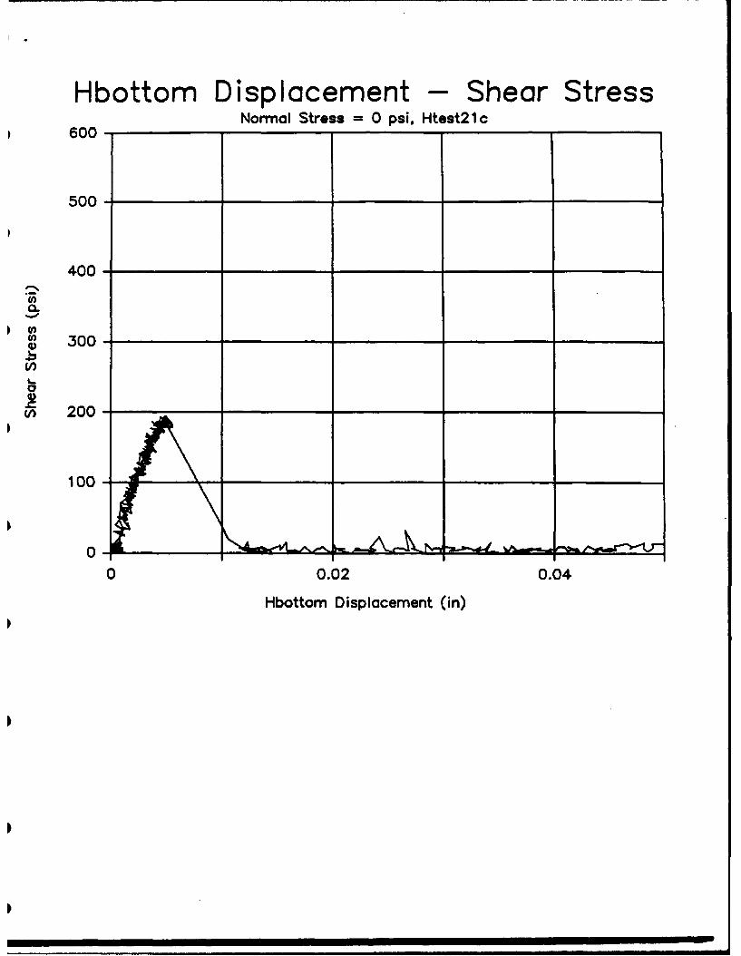
Hbottom Displacement - Shear StressNormal Stress =0 psi, Htest2l c
600-
500-
400-
S300-(I)
C,200-
100 -
0-10 0.02 0.04
Hbottom Displacement (in)
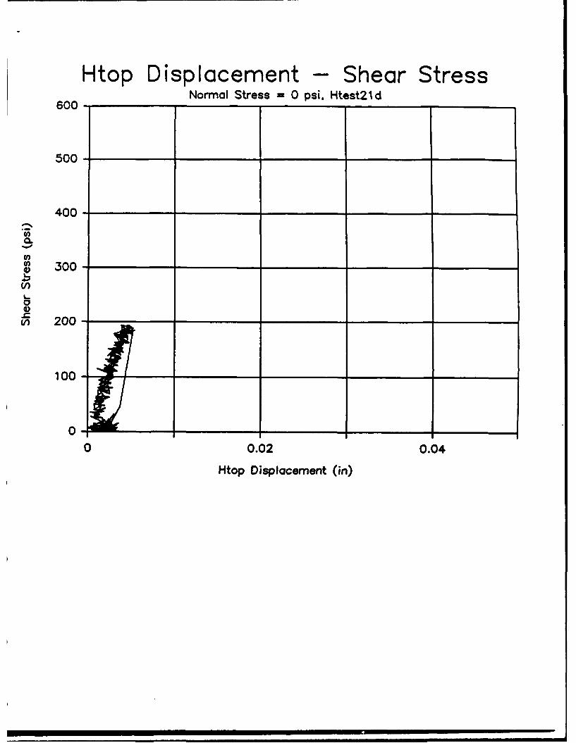
Htop Displacement - Shear StressNormal Stress =0 psi. Htest2l d
600-
500-
400-
C)
000
C')
3) 00-
100-
0-10 0.02 0.04
Htop, Displacement (in)

Shear Displacement-Normal DisplacementNormal Stress = 0 psi. Htest2lea
0.01 -
0.009 - _ _ _ _ _ _ _ _ _ _ _ _ _ _ _
0.008-
0.007- Y1C
S0.006 - _ _ _ _ _ _ _ _ _ _ _ _ _ _
Ck.
0 0.02 0.04
Shear Displacement (in)

Normal Displacement - Shear StressNormal Stress =0 psi, Htest22a
600-
500-
400-
C0
~, 300-
LI)
C,) 200 -
100-
0-0 0.02 0.04
Normal Displacement (in)
Fig. 14 (a) -(e) Load-displacement response diagramsfor test series 22
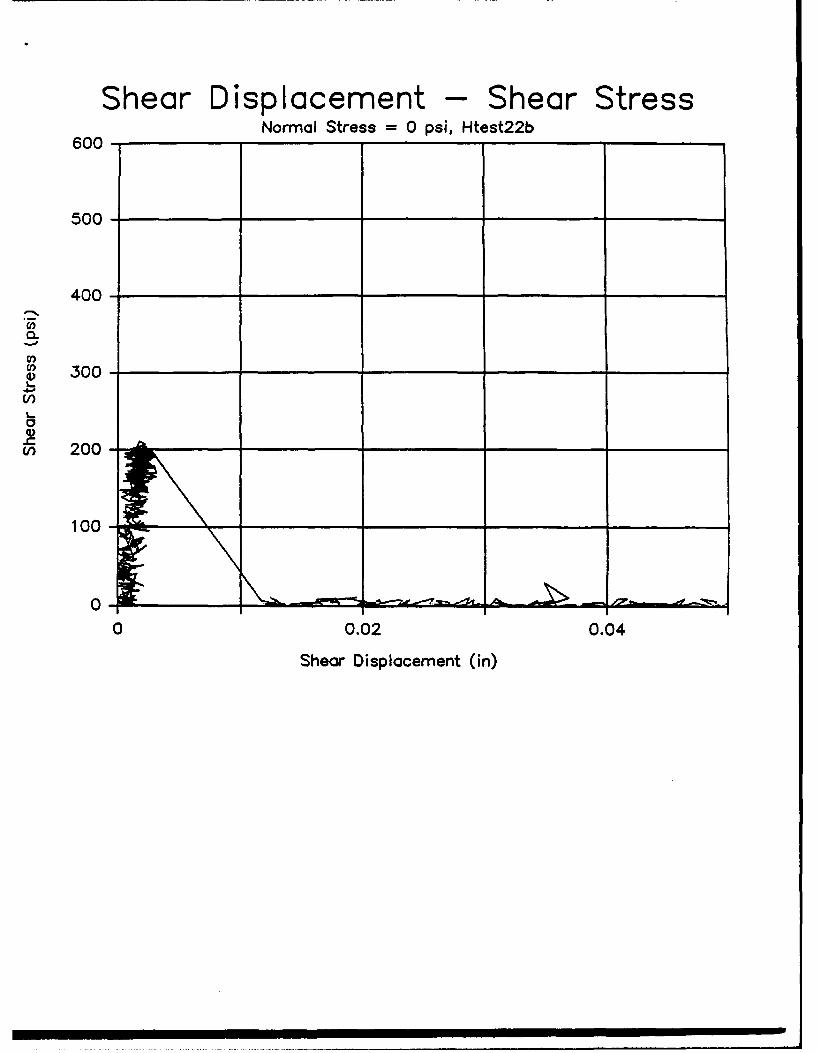
Shear Displacement - Shear StressNormal Stress = 0 psi, Htest22b
600-
500-
400-
o.
300-
- 200100
00
0 0.02 0.04
Shear Displacement (in)

Hbottomn Displacement - Shear Stress600-Normal Stress =0 psi, Htest22c
600-
500-
400-
100-
00
0 0.02 0.04
Hbottomn Displacement (in)
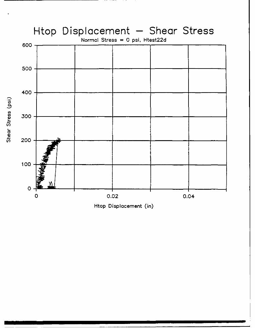
Htop Displacement - Shear Stress
600-Normal Stress =0 psi, Htest22d
500-
400-
-0
1 300 -I
U')
&' 200-
100-
0-10 0.02 0.04
Htop Displacement (in)

Shear Displacement-Normal Displacement0.01 - ____ __ Normal Stress = 0 psi, Htest22e
0.009 - _ _ _ _ _ _ _ _ _ _ _ _ _ _ _
0.008 -
S0.007-
0E
0.005-
0.001-
00
0 0.02 0.04
Shear Displacement (in)

Normal Displacement - Shear StressNormal Stress =+25 psi, Htest23a
600-
500-
400-
300
VC)
2 :00-
10
0-1
0 0.02 0.04
Normal Displacement (in)
Fig. 15 (a) -(f) Load-displacement response diagramsfor test series 23

Shear Displacement - Shear StressNormal Stress =+25 psi, Htest23b
600-
500-
400-
C,)
0.0
0 .0 00
C,) ~ ~ ~ ~ ~ ha Displacement_ (in)____ ______

Hbattom Displacement - Shear Stress600 _________Normal
Stress =+25 psi, Htest23c
500 -
400-
U)
100
1 L
0 0.02 0.04
Hbottomn Displacement (in)
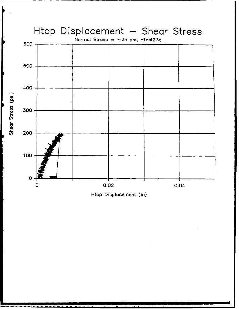
Htop Displacement - Shear StressNormal Stress =+25 psi, Htest23d
600-
500-
400-
0.
300-
V) 200-
100 - _ _ _ _ _ _ _ _ _ _ _ _
0-10 0.02 0.04
Htop Displacement (in)

Shear Displacement-Normal DisplacementNormal Stress =+25 psi, Htest23e
0.01 - _ _ _ _ _ _ _ _ _ _ _ _ _ _
0.009 -_ _ _ _ _ _ _ _ _ _
0.008 - _ _ _ _ _ _ _ _ _ _
0.007 - ___
C
S0.006 - _ _ _ _ _ _ _ _ _ _ _ _ _ _ _ _ _ _ _ _ _ _ _
E
0z
0.002-
0.001if
0 0.02 0.04
Shear Displacement (in)
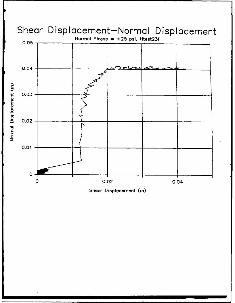
Shear Displacement-Normal Displacement0.05-Normal Stress = +25 psi, Htest23f
0.04 - _ _ _ _ _ _ _ _ _ _
C
S0.03-ECL
S0.02-
0.01 - _ _ _ _ _ __ _ _ _ _
0-
0 0.02 0.04
Shear Displacement (in)

Normal Displacement- Shear StressNormal Stress = +25 psi, Htest24a
600 -
500-
400-
C')-0-300-
V)
V) 200-
00
1~ 00-
0 0.02 0.04
Normal Displacement (in)
Fig. 16 (a) - (e) Load-displacement response diagramsfor test series 24
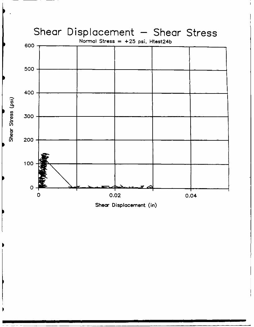
Shear Displacement - Shear Stress600-Normal Stress =+25 psi, Htest24b
600-
500-
200-
1, 00
00
0 0.02 0.04
Shear Displacement (in)
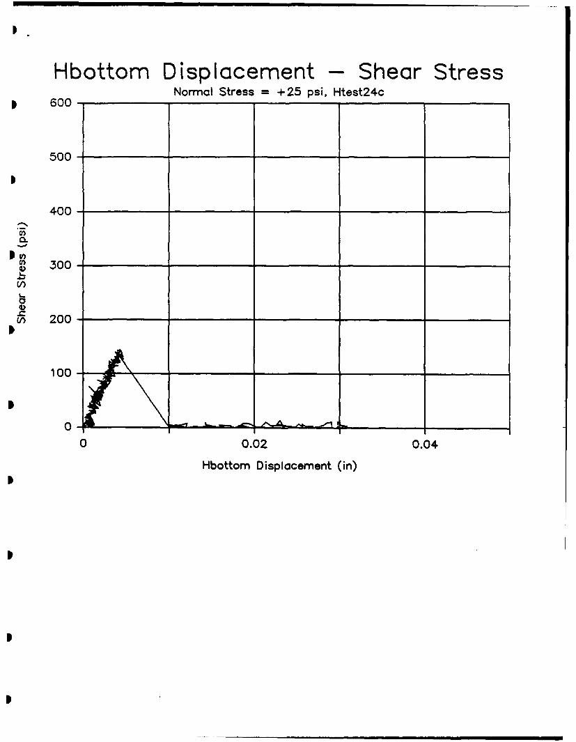
Hbottomn Displacement -Shear StressNormal Stress =+25 psi, Htest24c
* 600-
500-
400-
300
200
100-
LJ.L0.
0 0.02 0.04
Hbottom Displacement (in)
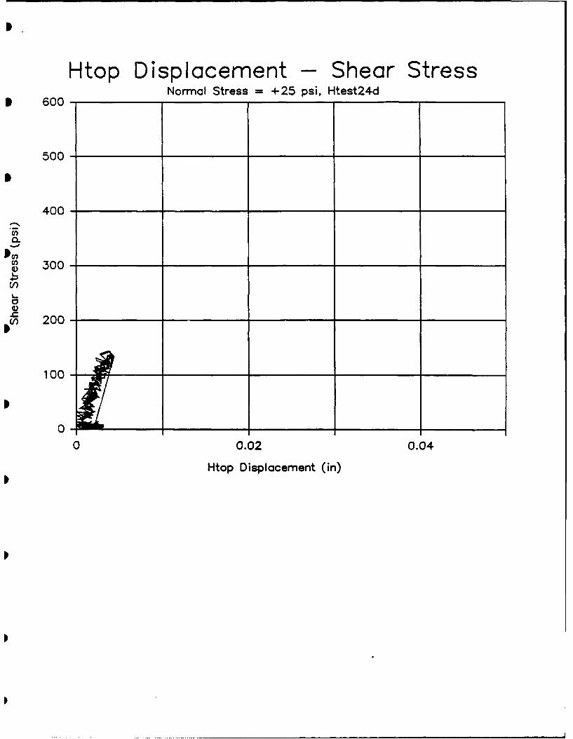
Htop Displacement - Shear StressNormal Stress =+25 psi, Htest24d
* 600-
500-__ _ _ _
400 _ _ __ _ _
300
100-
000 .0)00
-c ~ ~ ~ ~ ~ ~ ~ Ho Displacemen (in)__ _ _ __ _ _ __ _ _ __ _ _ _
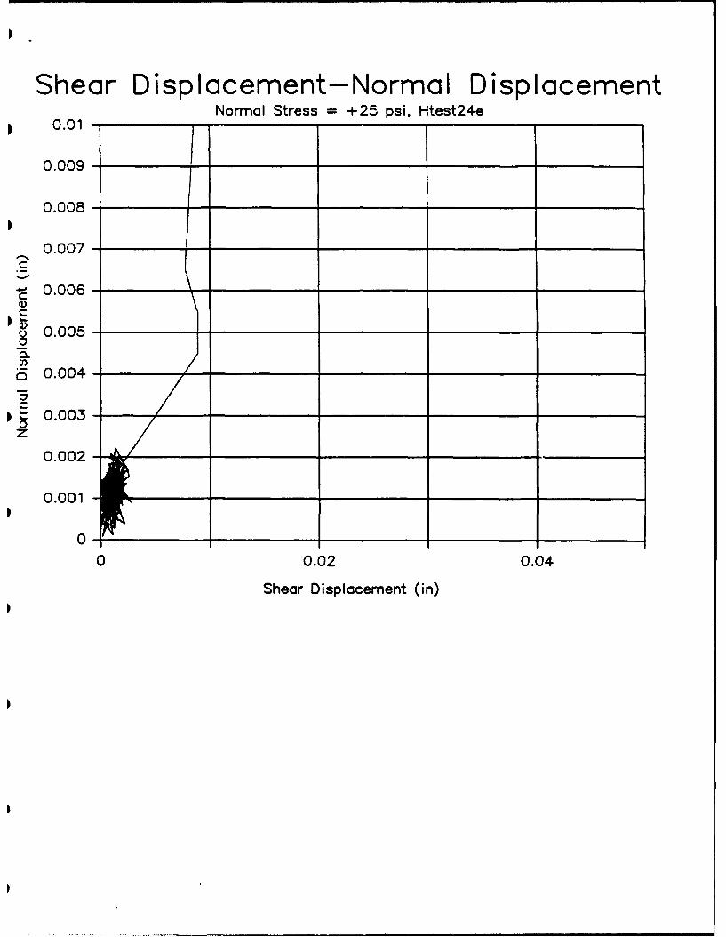
Shear Displacement-Normal DisplacementNormal Stress =+25 psi, Htest24e
0.01 -
0.009 - _ _ _ _ _ _ _ _ _ _
0.008 -
0.007 -
- ~0.006 - _ _ _ _ _ _ _ _ _ _ _ _ _ _ _
0.04
0.03
0.0z
0.001
00 0.02 0.04
Shear Displacement (in)
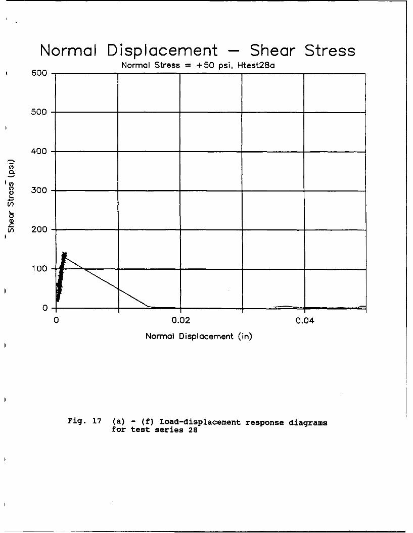
Normal Displacement - Shear Stress600-Normal Stress =+50 psi. Htest28a
500-
400-
300
1 00-
00
0 0.02 0.04
Normal Displacement (in)
Fig. 17 (a) -(f) Load-displacement response diagramsf or test series 28
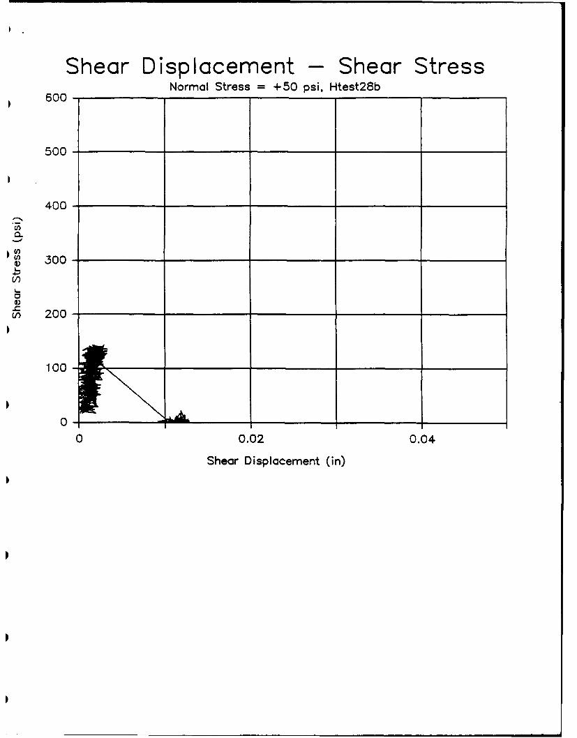
Shear Displacement - Shear StressNormal Stress =+50 psi, Htest28b
600 -
500-
400-
L
30
V) 200-
0-0 0.02 0.04
Shear Displacement (in)
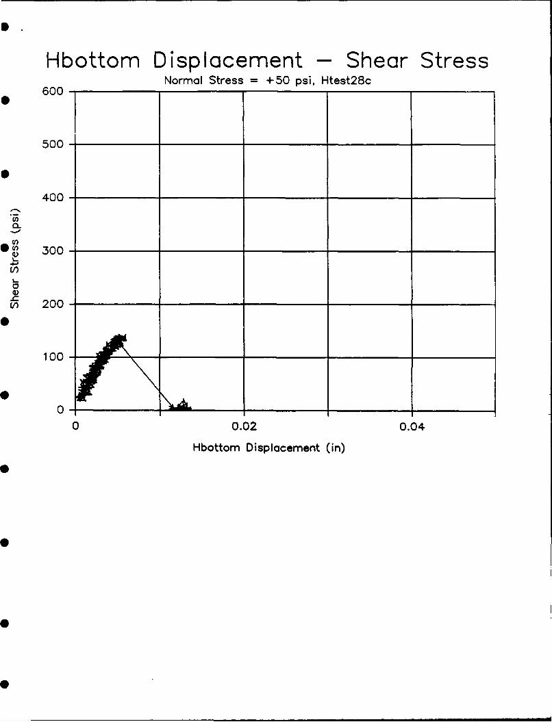
Hbottom Displacement - Shear StressNormal Stress =+50 psi, Htest28c
600-J
500-
400-
300
t) 200~
00
0 __0 __ . __
Hbottom Displacement (in)
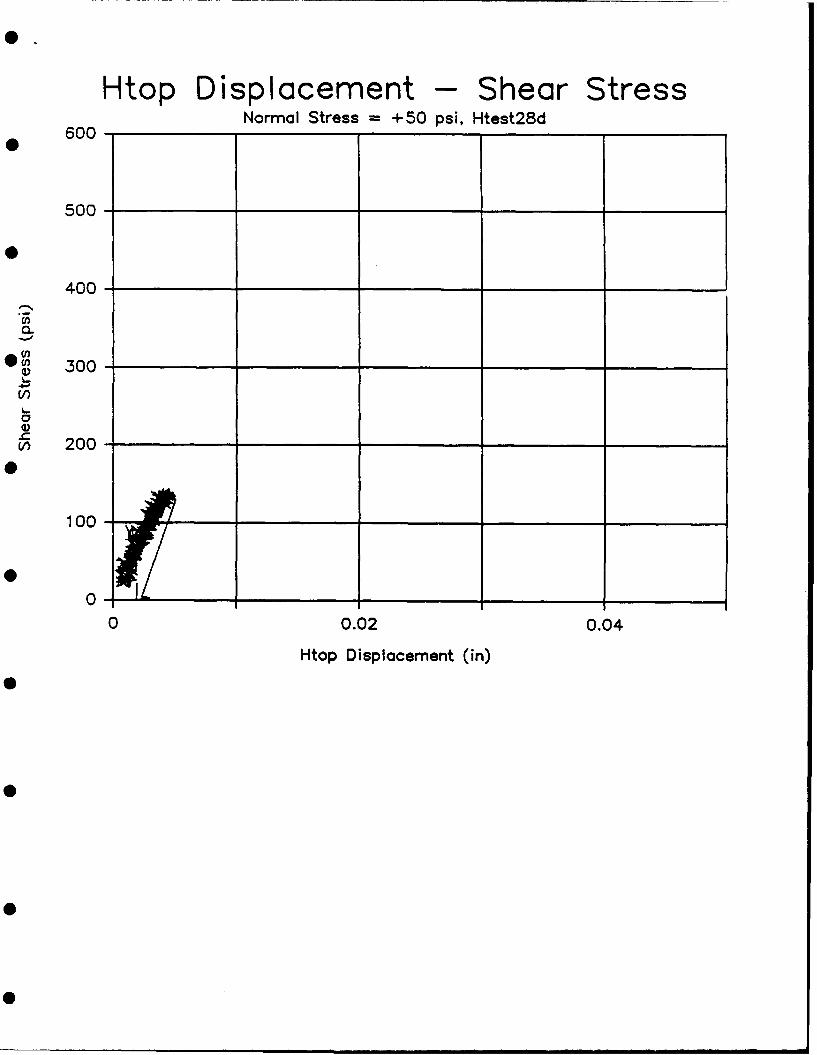
Htop Displacement - Shear StressNormal Stress =+50 psi, Htest28d
600-
500-
0
100-
0.0
0 0.000-0
HtpDslceet(n
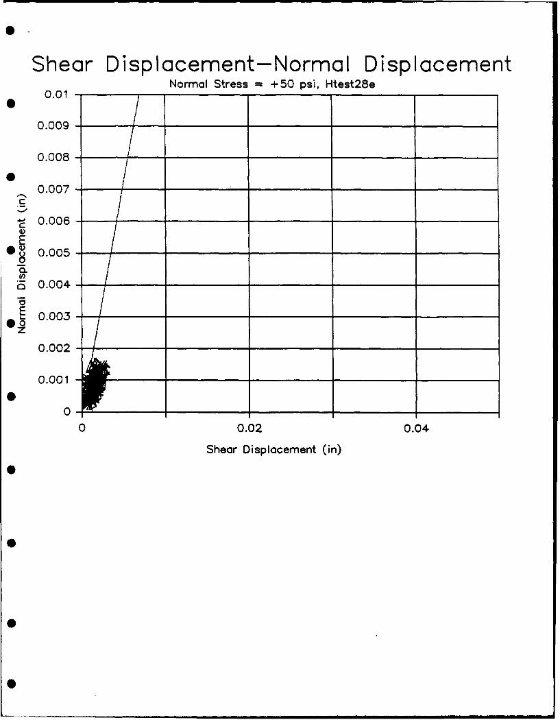
Shear Displacement-Normal DisplacementNormal Stress - +50 psi, Htest28e
0.01
0.009
0.008-
0.007-
C
C 0.006 -QE
0.005-
000
0 0.02 0.04
Shear Displacement (in)
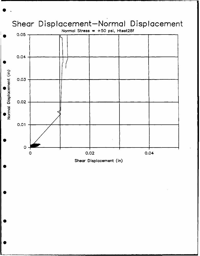
Shear Displacement-Normal D isp lacementNormal Stress + +50 psi, Htest28f
* 0.05-
0.04 - _ _ _ _ _ __ _ _ _
0E
o 0.02-
E
0.0
0-0 0.02 0.04
Shear Displacemnent (in)
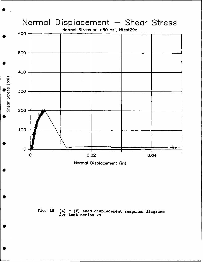
Normal Displacement - Shear StressNormal Stress =+50 psi, Htest29a
600 -
500-
400-
300
V)
V) 20
1 00 -
00
0 0.02 0.04
Normal Displacement (in)
Fig. 18 (a) -(f) Load-displacement response diagramsfor test series 29
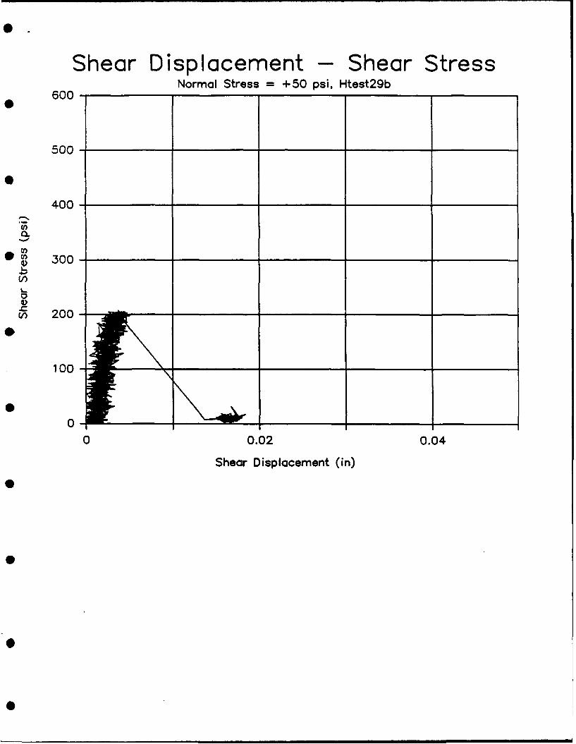
Shear Displacement - Shear Stress600-Normal Stress =+50 psi, Htest29b
600-
500-
00
200-
*~ 100-
00
0 0.02 0.04
Shear Displacement (in)
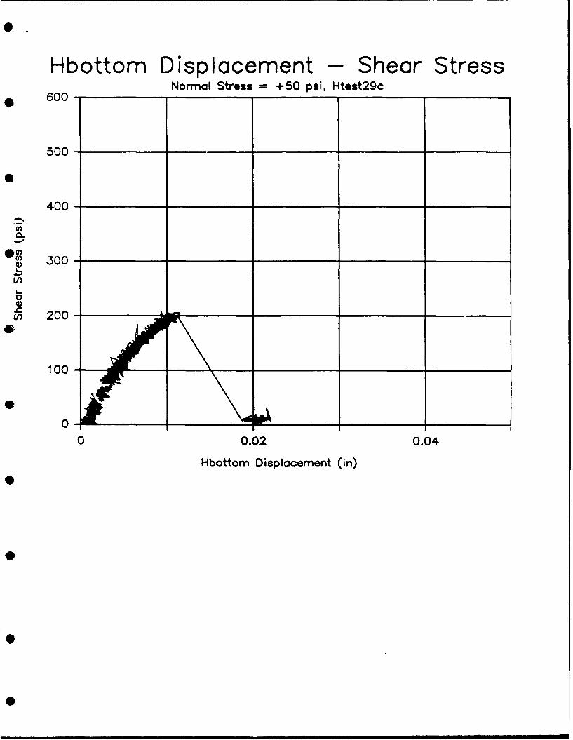
Hbottom Displacement - Shear StressNormal Stress =+50 psi, Htest29c
600-
500-
400-
0.
S300-
V
u 200-
100 - _ _ _ _
0-440 0.02 0.04
Hbottom Displacement (in)

Htop Displacement -Shear StressNormal Stress =+50 psi, Htest29d
* 600-
500-
400 _ _ __ _ _
0.
~, 300-
V)
100
0)0
0C 0.02_0.04
Htp 200-ceen (n
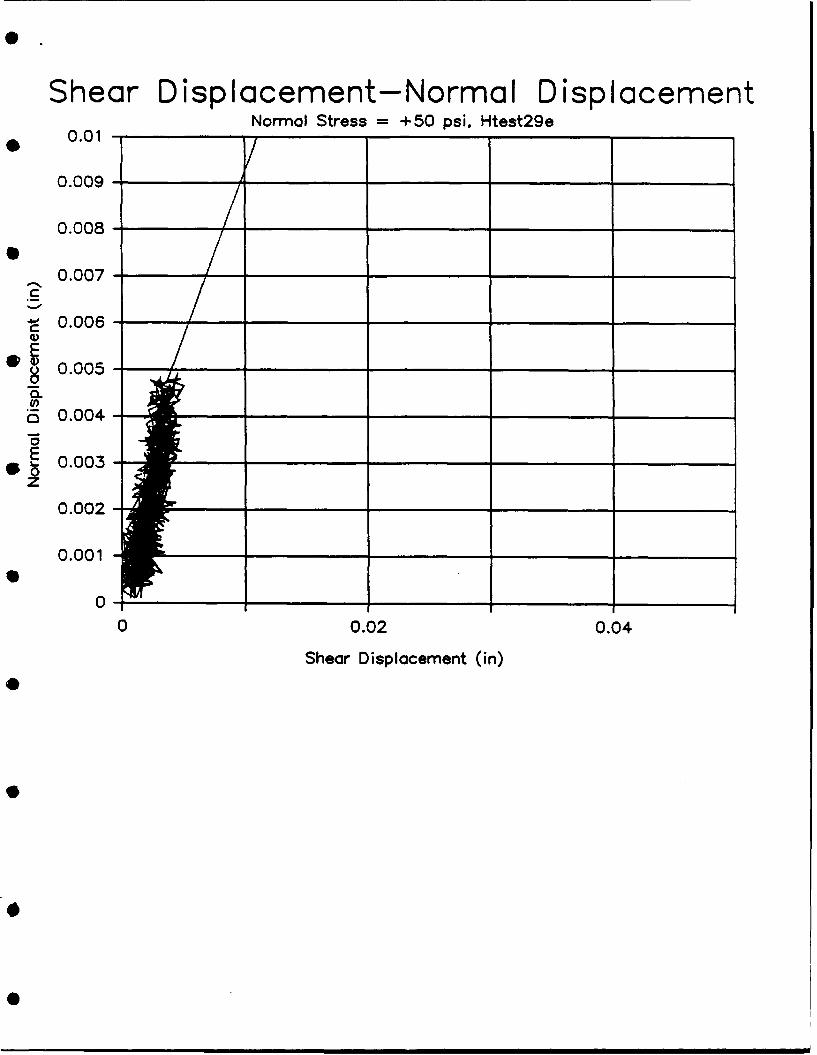
Shear Displacement-Normal D isp lacementNormal Stress =+50 psi, Htest29e
0 0.01 -
0.009 - _ _ _ _ _ _ _ _ _ _ _ _ _ _
0.008 - _ _ _ _ _ _ _ _ _ _
0.007 -
C
C 0.006 - _ _ _ _ _
E0.005-
S0.004
* 0.003-z
0.002
0.001_ __
00 0.02 0.04
Shear Displacement (in)
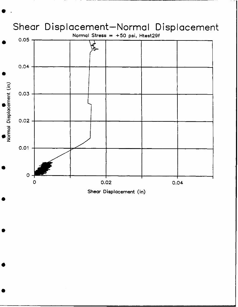
Shear Displacement-Normal Displacement0.05-Normal Stress =+50 psi, Htest29f
0.04 -
C
~-W 0.03-C
0.
S0.02-
so
0.01 - _ _ _ _ _ _ _ _ _ _
0 0.02 0.04
Shear Displacement (in)

Normal Displacement - Shear StressNormal Stress =+75 psi, Htest.30a
600-
500-
400
400-
0~0
fo ts sres3
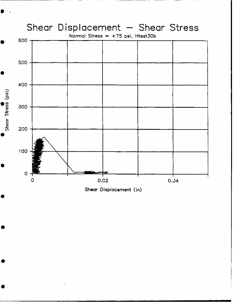
Shear Displacement - Shear Stress600 -Normal Stress =+75 psi, Htest3Ob
600-
400-
0L-0
~, 300-
V)
0r 200-
100-
00
0 0.02 0.'J4
Shear Displacement (in)
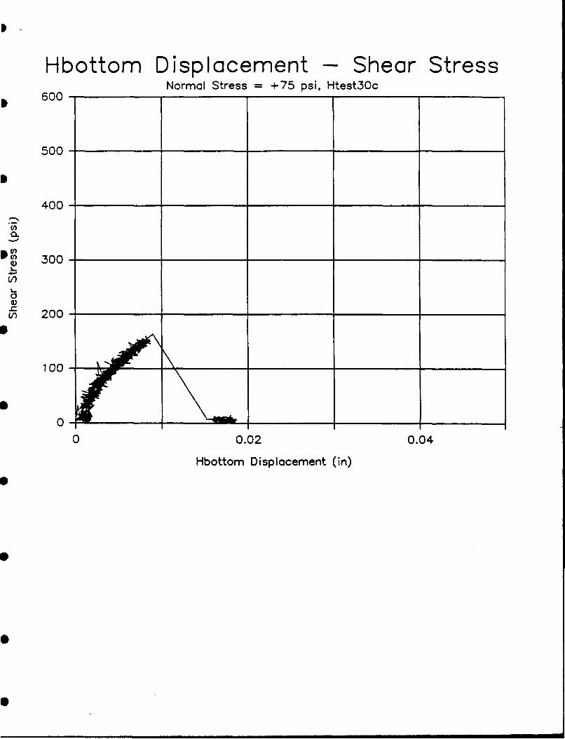
Hbottom Displacement - Shear StressNormal Stress =+75 psi, Htest30c
600 -
500-
400-
0.
100-
L.r
00
0 0.02 0.04
Hbottom Displacement (in)
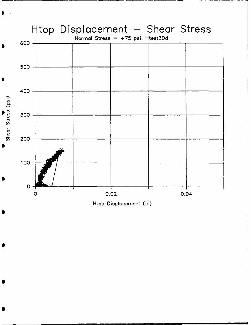
Htop Displacement - Shear StressNormal Stress =+75 psi, Htest3Od
600 -
500-
400-
C,
S300-V)
20
1 00- _ _ _ _
00 0.02 0.04
Htop Displacement (in)
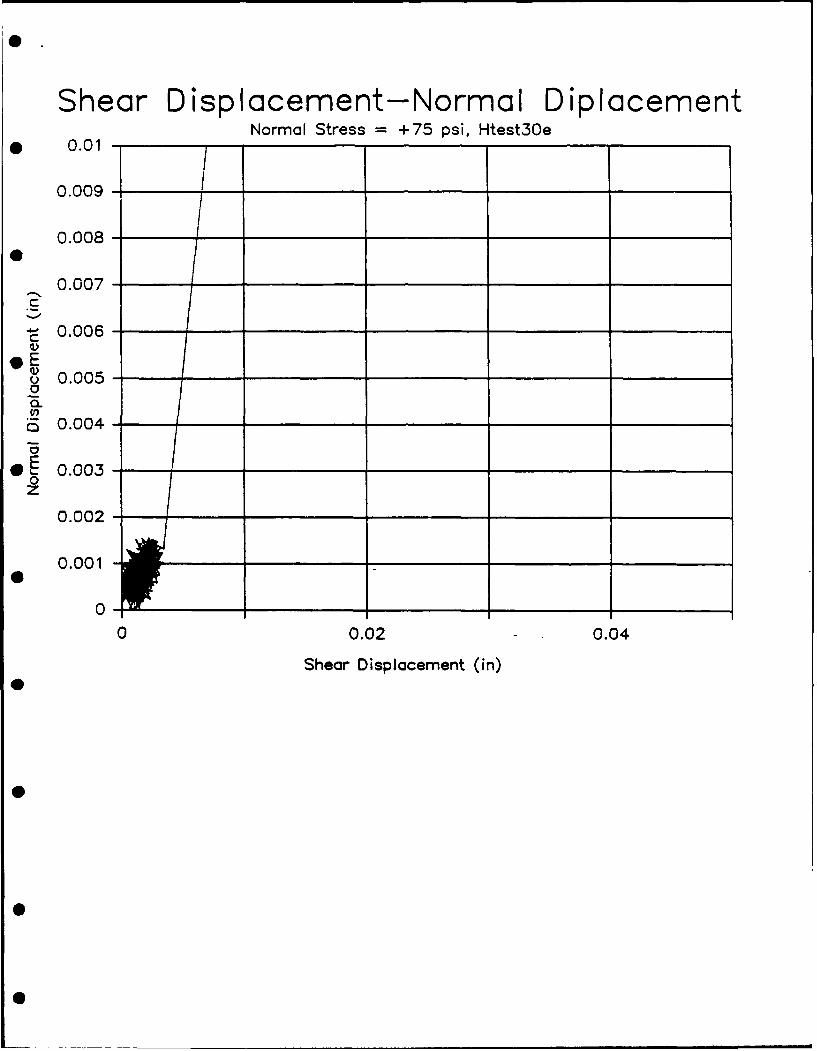
Shear Displacemnent-Normal DiplacemnentNormal Stress =+75 psi, Htest30e
* 0.01-
0.009 -,
0.008 -
0.007C
A- 0.006 -
u 0.005 - _ _ _ _ _ _ _ _ _ _
*S 0.004 -
0E0.003-0
0.002-
0.001
00 0.02 0.04
Shear Displacement (in)
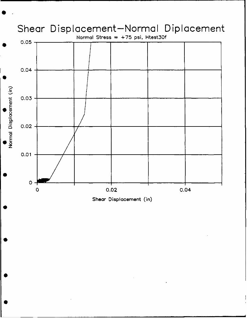
Shear Displacement-Normal DiplacementNormal Stress =+75 psi, Htest30f
0.05-
C'0.03-
0.0
0 ,
0 0.02-.0
Sha.islcmet(n

Normal Displacement - Shear Stress600-Normal Stress =+100 psi, Htest3l a
500-
400-
'0
q~300-
.
V) 200-
100
00
0 0.02 0.04
Normal Displacement (in)
Fig. 20 (a) -(f) Load-displacement response diagramsfor test series 31
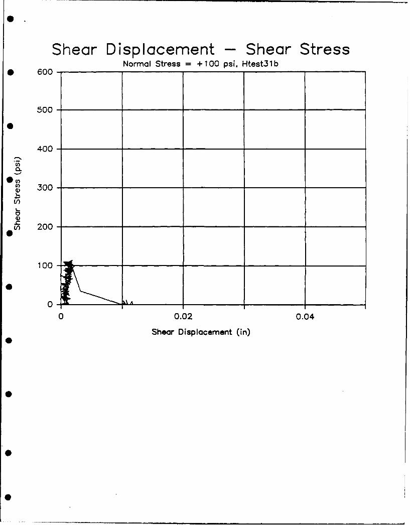
Shear Displacement -Shear StressNormal Stress + +100 psi, Htest3l b
* 600-
500-
400-
~" 300-(I)
V)200-
00
0-0 0.02 0.04
Shear Displacement (in)
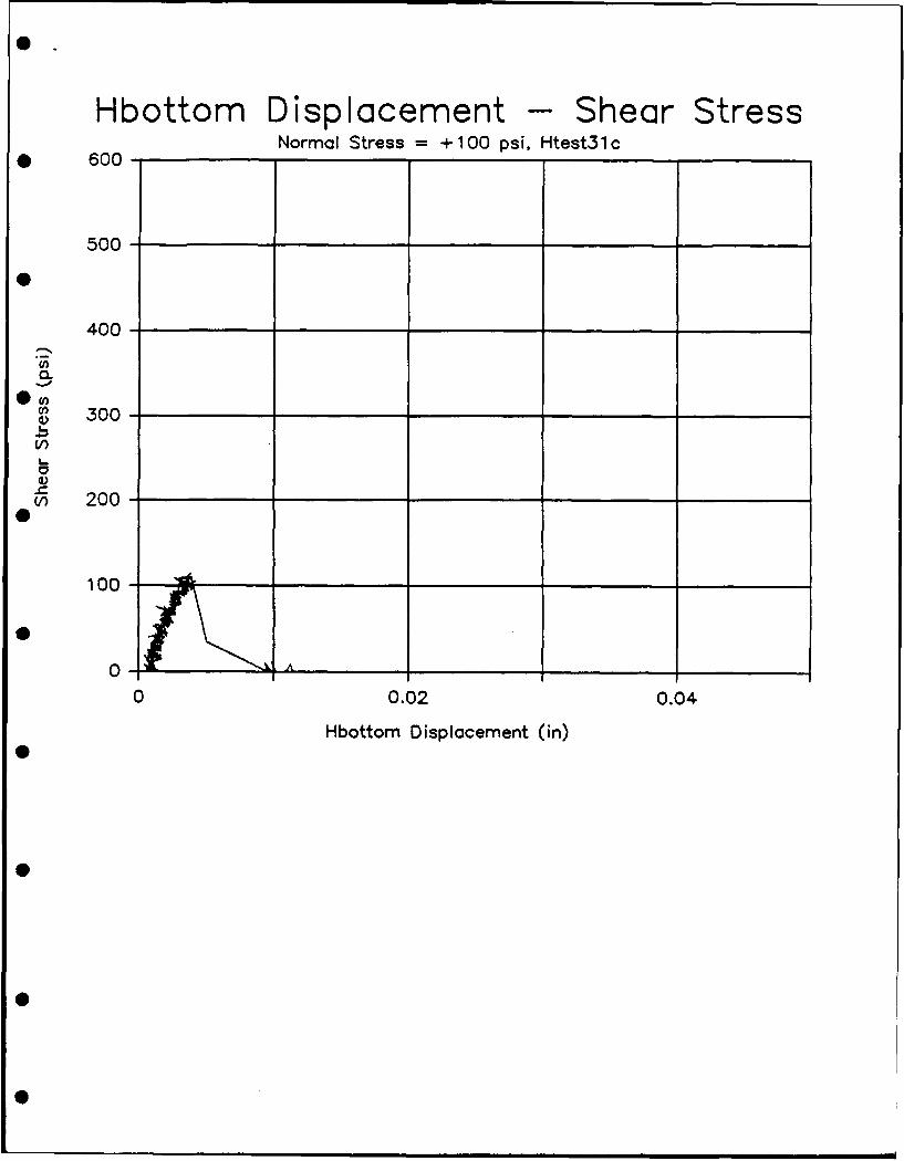
Hbottom Displacement - Shear StressNormal Stress = +100 psi, Htest3l c
* 600-
500-
400-
o 300-
V)L
V) 200-
100
0
0 0.02 0.04
Hbottom Displacement (in)
0
0
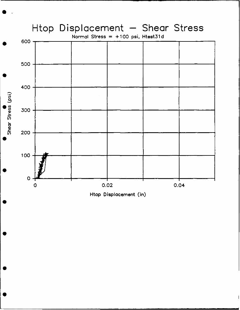
Htop Displacement - Shear StressNormal Stress + +100 psi, Htest3l d
600- ____
500-
000
400-
En
200
100-
0-1110 0.02 0.04
Htop Displacement (in)
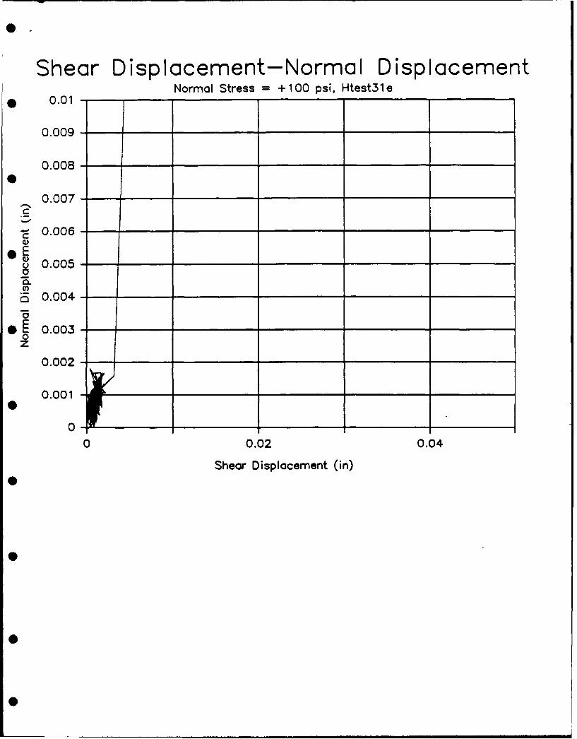
Shear Displacement-Normal DisplacementNormal Stress + +100 psi, Htest3l e
* 0.01 -
0.009--
0.008 -
0.07
0.0076-
C-0.006 4_____ _____ _____
8 0.003 - _ _ _ _ _ _ _ _ _ _ _ _ _ _
o 0.001 _ _ _ _ _ _ _ _ _ _
00
0 0.02 0.04
Shear Displacement (in)

Shear Displacement-NormalI DisplacementNormc'I Stress + +100 psi, Htest3l f
*0.05-/ _ _ _ _ _ _ _ _ _ _ _ _
0.04-
C
.W- 0.03-
C',
6 0.02-
0
0-0 0.02 0.04
Shear Displacement (in)
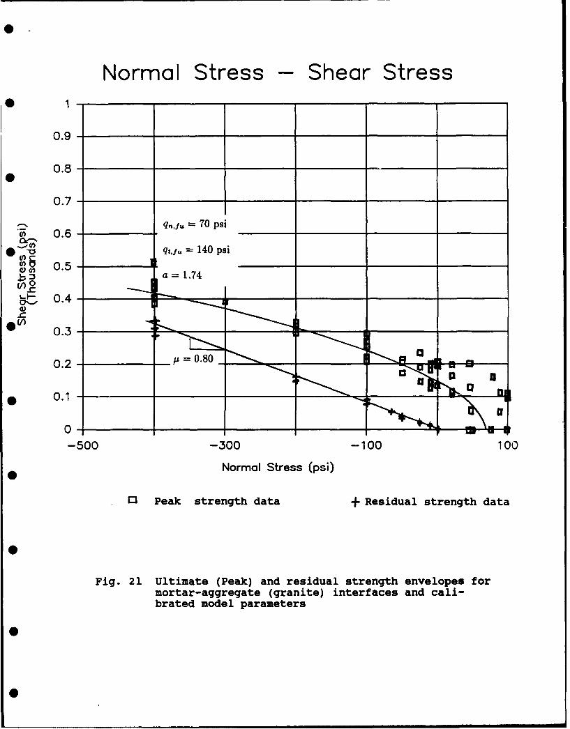
Normal Stress -Shear Stress
0.9 -
0.8-
0.7-
0.6 - ___________70 psi______
* qt,f. 140 psi0~0 A_ _ _ _ _ _ _ _ _ _ _
V 0.5-V) 0-C
__ 0.4-.C
60 0.3-
0.2-0.0t
* 0.1 -
0-
-500 -300 -100 100
Normal Stress (psi)
0 Peak strength data + Residual strength data
Fig. 21 Ultimate (Peak) and residual strength envelopes formortar-aggregate (granite) interfaces and cali-brated model parameters
0