Embed Size (px)
Citation preview
8/7/2019 ad24aMODULE 2B- OR
http://slidepdf.com/reader/full/ad24amodule-2b-or 1/25
AIBS
1
AIBSMBA-IB, MIB 201
OPERATIONS RESEARCH
REMICAAGGARWAL
8/7/2019 ad24aMODULE 2B- OR
http://slidepdf.com/reader/full/ad24amodule-2b-or 2/25
AIBS
2
InventoryManagement
8/7/2019 ad24aMODULE 2B- OR
http://slidepdf.com/reader/full/ad24amodule-2b-or 3/25
AIBS
3
• Economic order quantity model• Economic production model
• Quantity discount model
Economic Order QuantityModels
8/7/2019 ad24aMODULE 2B- OR
http://slidepdf.com/reader/full/ad24amodule-2b-or 4/25
AIBS
4
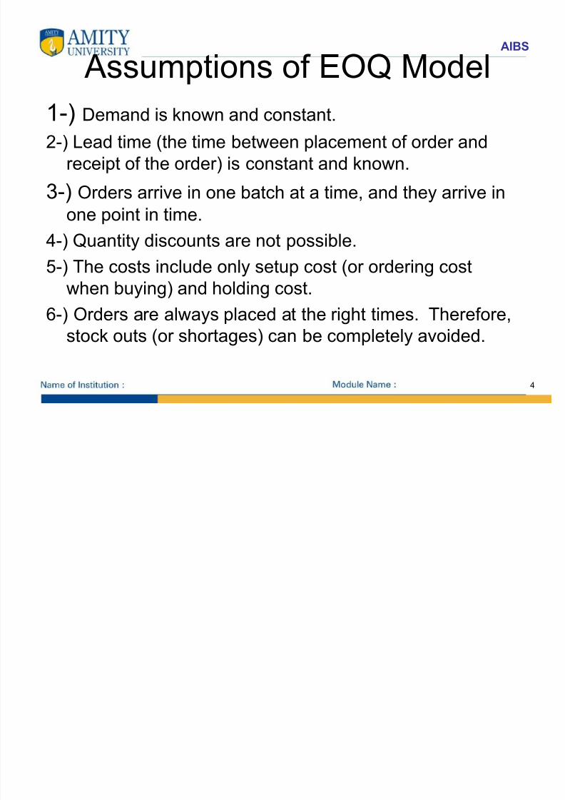
Assumptions of EOQ Model1-) Demand is known and constant.
2-) Lead time (the time between placement of order andreceipt of the order) is constant and known.
3-) Orders arrive in one batch at a time, and they arrive inone point in time.
4-) Quantity discounts are not possible.
5-) The costs include only setup cost (or ordering cost
when buying) and holding cost.6-) Orders are always placed at the right times. Therefore,
stock outs (or shortages) can be completely avoided.
8/7/2019 ad24aMODULE 2B- OR
http://slidepdf.com/reader/full/ad24amodule-2b-or 5/25
AIBS
5
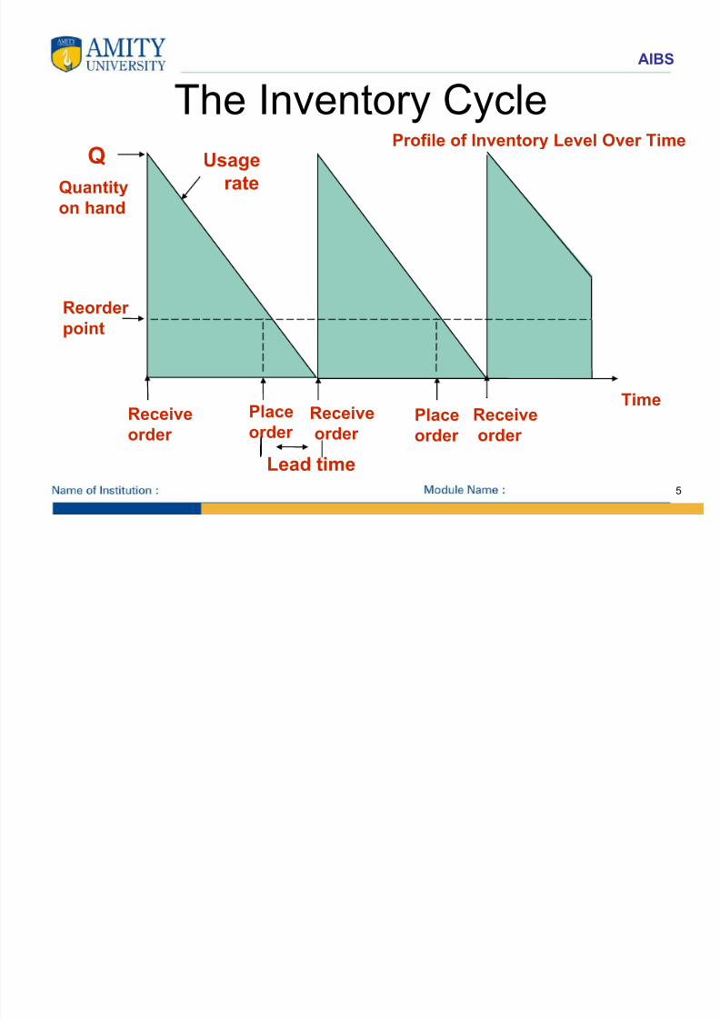
The Inventory CycleProfile of Inventory Level Over Time
Quantity
on hand
Q
Receive
order
Place
order Receive
order Place
order
Receive
order
Lead time
Reorder
point
Usage
rate
Time
8/7/2019 ad24aMODULE 2B- OR
http://slidepdf.com/reader/full/ad24amodule-2b-or 6/25
AIBS
6
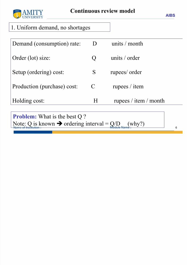
Continuous review model
1. Uniform demand, no shortages
Demand (consumption) rate: D units / month
Order (lot) size: Q units / order
Setup (ordering) cost: S rupees/ order
Production (purchase) cost: C rupees / item
Holding cost: H rupees / item / month
Problem: What is the best Q ?
Note: Q is known ordering interval = Q/D (why?)
8/7/2019 ad24aMODULE 2B- OR
http://slidepdf.com/reader/full/ad24amodule-2b-or 7/25
AIBS
7
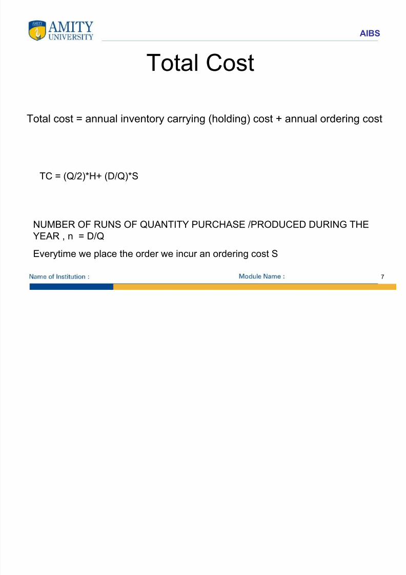
Total CostTotal cost = annual inventory carrying (holding) cost + annual ordering cost
TC = (Q/2)*H+ (D/Q)*S
NUMBER OF RUNS OF QUANTITY PURCHASE /PRODUCED DURING THEYEAR , n = D/Q
Everytime we place the order we incur an ordering cost S
8/7/2019 ad24aMODULE 2B- OR
http://slidepdf.com/reader/full/ad24amodule-2b-or 8/25
AIBS
8
Cost Minimization Goal
Order Quantity
(Q)
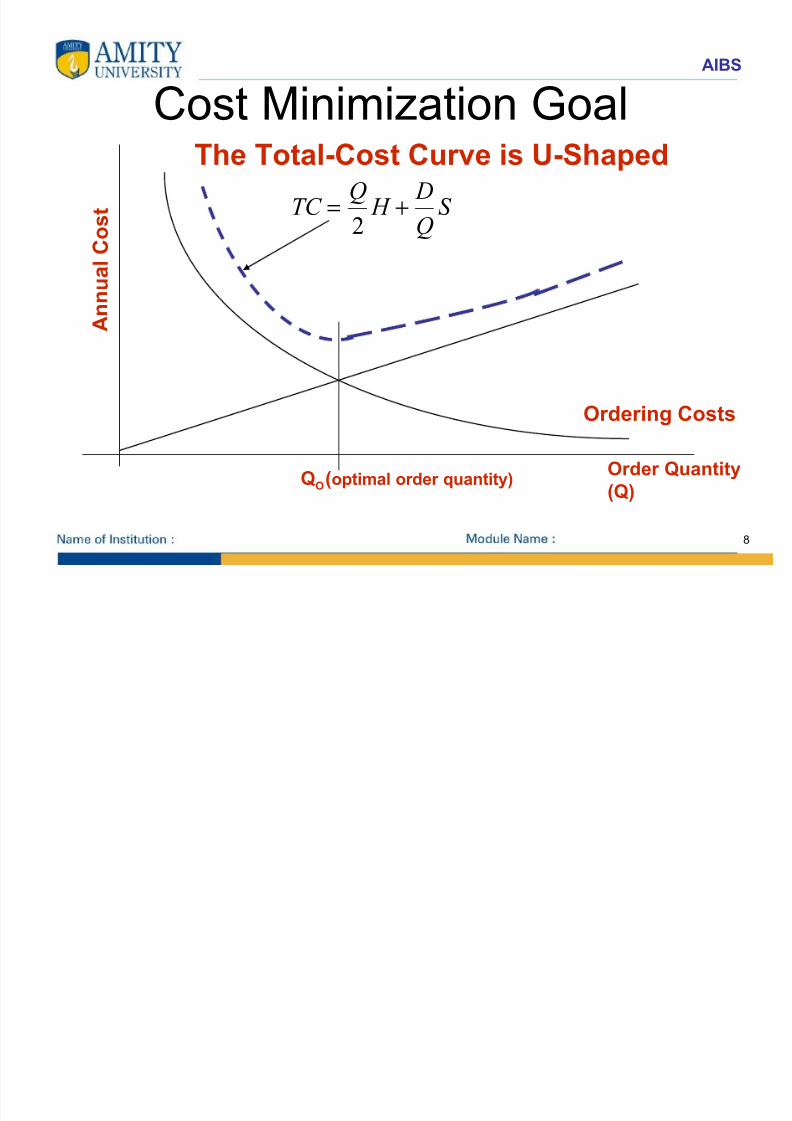
The Total-Cost Curve is U-Shaped
Ordering Costs
QO
Annua l
Cost
(optimal order quantity)
TC Q
H D
QS = +
2
8/7/2019 ad24aMODULE 2B- OR
http://slidepdf.com/reader/full/ad24amodule-2b-or 9/25
AIBS
9
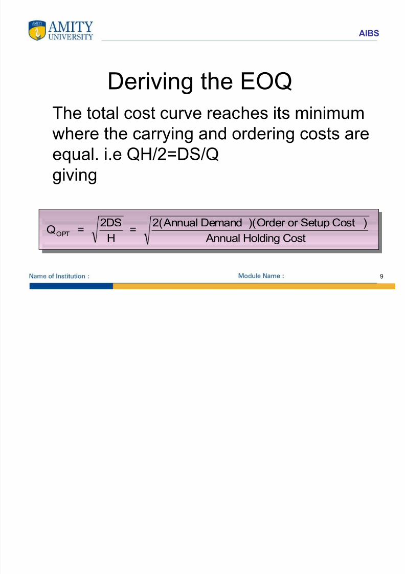
Deriving the EOQThe total cost curve reaches its minimum
where the carrying and ordering costs areequal. i.e QH/2=DS/Qgiving
Q =2DS
H=
2(Annual Demand )(Order or Setup Cost )
Annual Holding CostOPT
8/7/2019 ad24aMODULE 2B- OR
http://slidepdf.com/reader/full/ad24amodule-2b-or 10/25
AIBS
10
Lead time
• There is a time between placement and
receipt of an order.• This is called LEAD TIME or delivery time.
8/7/2019 ad24aMODULE 2B- OR
http://slidepdf.com/reader/full/ad24amodule-2b-or 11/25
AIBS
11
Considering the Reorder Point
• ROP (in units) = (Demand Per Day) *(Lead time for a new order in days)
• ROP = d * L
8/7/2019 ad24aMODULE 2B- OR
http://slidepdf.com/reader/full/ad24amodule-2b-or 12/25
AIBS
12
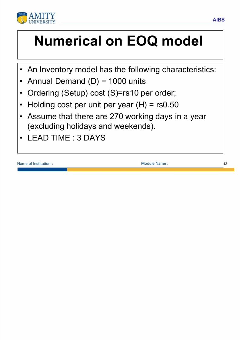
Numerical on EOQ model
• An Inventory model has the following characteristics:
• Annual Demand (D) = 1000 units• Ordering (Setup) cost (S)=rs10 per order;
• Holding cost per unit per year (H) = rs0.50
• Assume that there are 270 working days in a year (excluding holidays and weekends).
• LEAD TIME : 3 DAYS
8/7/2019 ad24aMODULE 2B- OR
http://slidepdf.com/reader/full/ad24amodule-2b-or 13/25
AIBS
13
• Questions:
a) Find the Economic Order Quantity (Q*) for thisinventory model.
b) How many orders should be placed during oneyear?c) What is the expected time between two
consecutive orders?
d) What is the total annual cost of this inventorymodel?
e) what is the reorder point
8/7/2019 ad24aMODULE 2B- OR
http://slidepdf.com/reader/full/ad24amodule-2b-or 14/25
AIBS
14
• Answers:
a) Q* = √[2(1000)10 / .50] = 200 units
b) Expected number of orders placed duringthe year (N) = D / Q* = 1000 / 200 = 5times.
8/7/2019 ad24aMODULE 2B- OR
http://slidepdf.com/reader/full/ad24amodule-2b-or 15/25
AIBS
15
c) Expected time between orders (T) = (Workingdays in a year) / N = 270 / 5 = 54 days.
d) Total Annual Cost = Annual Setup Cost +Annual Holding Cost
= DS / Q* + (Q*)H / 2
= 1000 (10) / 200+ (200) (.50) / 2 = rs100e) Reorder point = (1000/270 )* L = (1000/270)*3
=11.1
When inventory level becomes 11 units, an Order should be placed.
8/7/2019 ad24aMODULE 2B- OR
http://slidepdf.com/reader/full/ad24amodule-2b-or 16/25
AIBS
16
Example 2
• Annual demand for an item is D =8000/year.
• This year there will be 200 working days ina year.
• Delivery of an order for this item takes 3working days (L = 3 days).
8/7/2019 ad24aMODULE 2B- OR
http://slidepdf.com/reader/full/ad24amodule-2b-or 17/25
8/7/2019 ad24aMODULE 2B- OR
http://slidepdf.com/reader/full/ad24amodule-2b-or 18/25
AIBS
18
• Answers:
a) Demand per day for this item (d) = 8000 /200 = 40 units / day.
b) ROP = d . L = 40 . 3 = 120 units.
When inventory level becomes 120 units, anOrder should be placed.
8/7/2019 ad24aMODULE 2B- OR
http://slidepdf.com/reader/full/ad24amodule-2b-or 19/25
AIBS
19
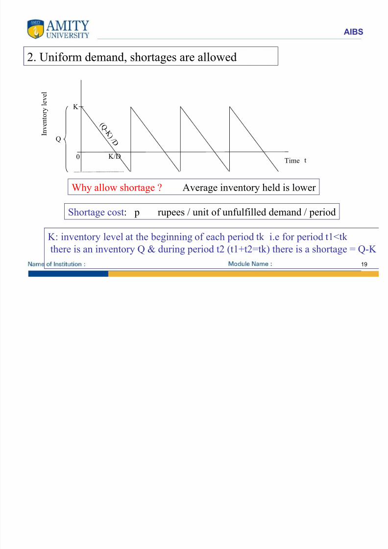
2. Uniform demand, shortages are allowed
In
ventory
level
Time t
Q
0
( Q - K ) / D
K
K/D
Shortage cost: p rupees / unit of unfulfilled demand / period
Why allow shortage ? Average inventory held is lower
K: inventory level at the beginning of each period tk i.e for period t1<tk
there is an inventory Q & during period t2 (t1+t2=tk) there is a shortage = Q-K
8/7/2019 ad24aMODULE 2B- OR
http://slidepdf.com/reader/full/ad24amodule-2b-or 20/25
AIBS
20
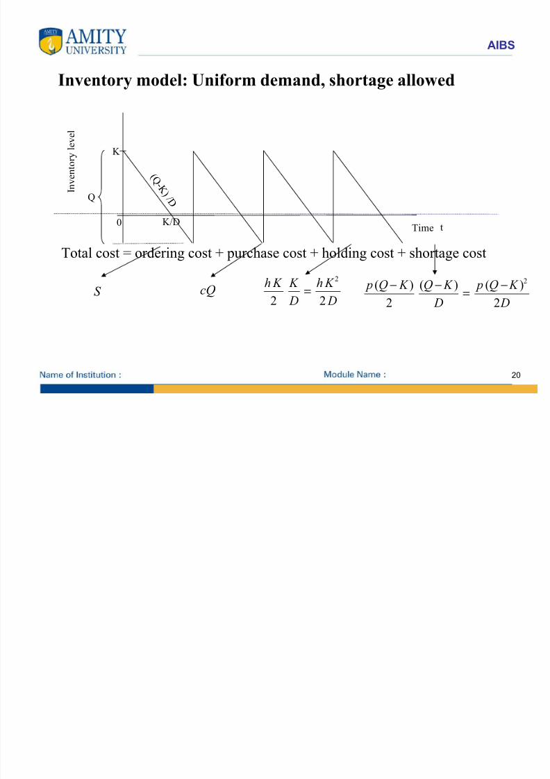
Inventory model: Uniform demand, shortage allowed
2
2 2
h K K h K
D D=
2( ) ( ) ( )
2 2
p Q K Q K p Q K
D D
− − −=
Total cost = ordering cost + purchase cost + holding cost + shortage cost
S cQ
In
ventory
level
Time t
Q
0
( Q - K ) / D
K
K/D
8/7/2019 ad24aMODULE 2B- OR
http://slidepdf.com/reader/full/ad24amodule-2b-or 21/25
AIBS
21
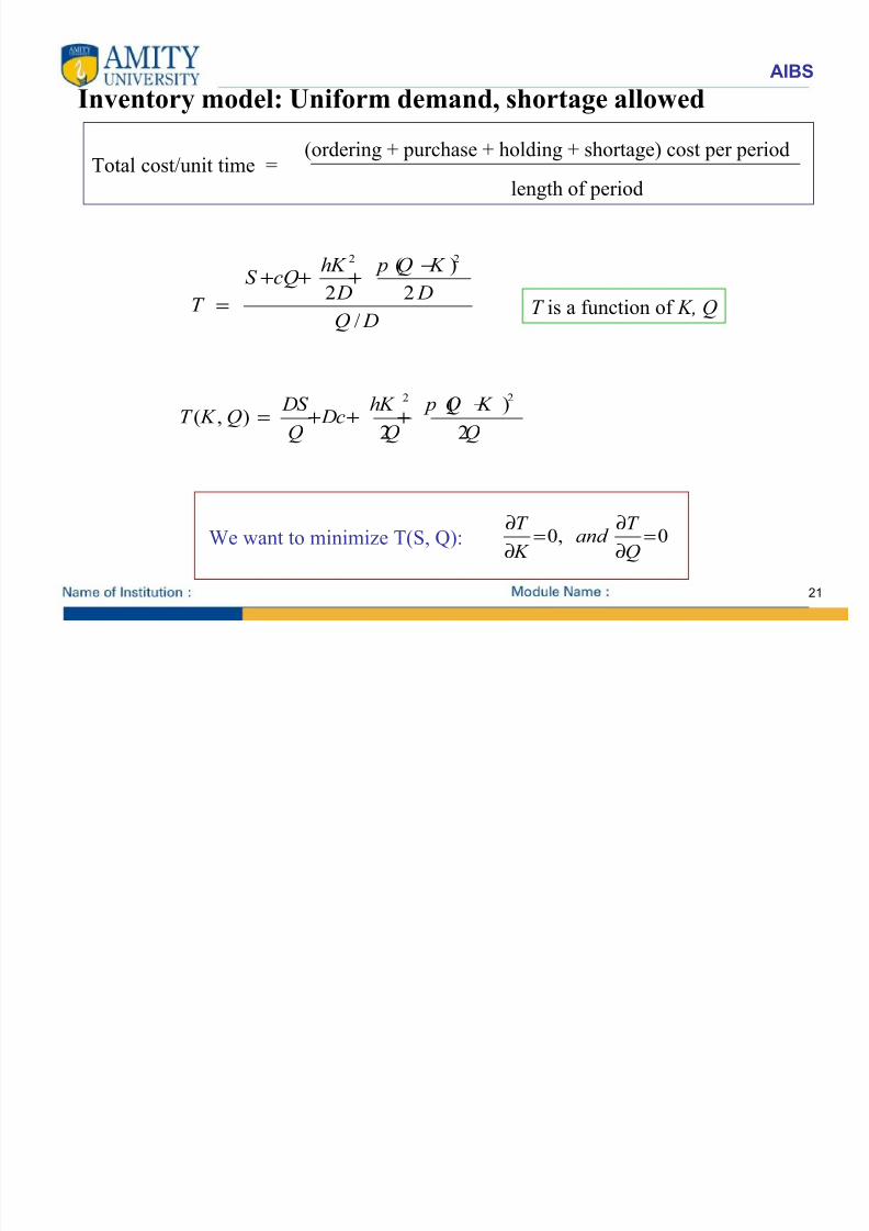
Inventory model: Uniform demand, shortage allowed
2 2( )
2 2/
hK p Q K S cQ
D DT Q D
−+ + +
=
2 2( )
( , )
2 2
DS hK p Q K T K Q Dc
Q Q Q
−= + + +
T is a function of K, Q
Total cost/unit time = (ordering + purchase + holding + shortage) cost per period
length of period
We want to minimize T(S, Q): 0, 0T T
and K Q
∂ ∂= =
∂ ∂
8/7/2019 ad24aMODULE 2B- OR
http://slidepdf.com/reader/full/ad24amodule-2b-or 22/25
AIBS
22
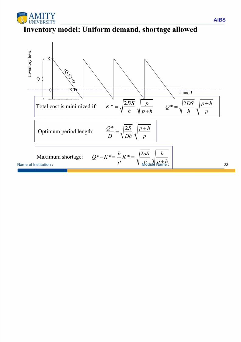
Inventory model: Uniform demand, shortage allowed
2*
DS pK
h p h=
+
2*
DS p hQ
h p
+=Total cost is minimized if:
Optimum period length:* 2Q S p h
D Dh p
+=
Maximum shortage:2
* * *h aS h
Q K K
p p p h
− = =
+
Inventory
level
Time t
Q
0
( Q - K
) / D
K
K/D
8/7/2019 ad24aMODULE 2B- OR
http://slidepdf.com/reader/full/ad24amodule-2b-or 23/25
AIBS
23
• Numerical on EOQ MODEL WITHSHORTAGES
8/7/2019 ad24aMODULE 2B- OR
http://slidepdf.com/reader/full/ad24amodule-2b-or 24/25
AIBS
24
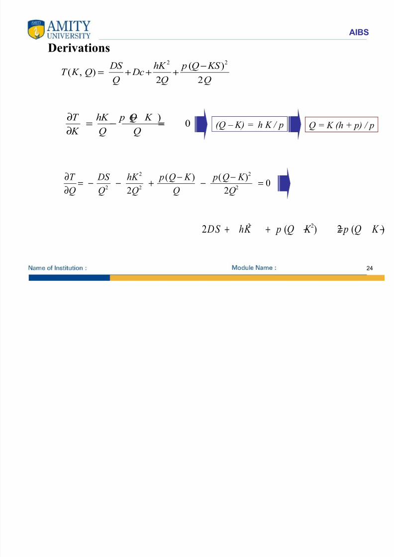
Derivations2 2
( )( , )2 2
DS hK p Q KS T K Q DcQ Q Q
−= + + +
( )0
T hK p Q K
K Q Q
∂ −= − =
∂
2 2
2 2 2
( ) ( )0
2 2
T DS hK p Q K p Q K
Q Q Q Q Q
∂ − −= − − + − =
∂
(Q – K) = h K / p
2 22 ( ) 2 ( )DS hK p Q K p Q K + + − = −
Q = K (h + p) / p
8/7/2019 ad24aMODULE 2B- OR
http://slidepdf.com/reader/full/ad24amodule-2b-or 25/25
AIBS
25
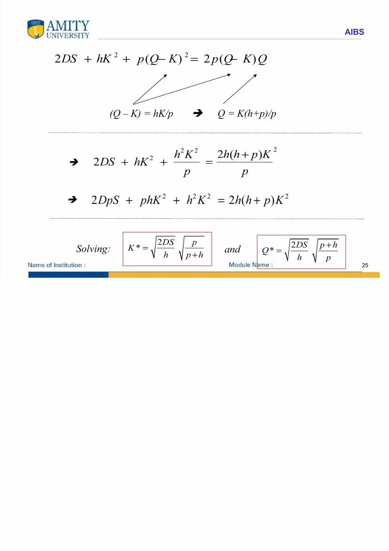
(Q – K) = hK/p Q = K(h+p)/p
Solving: and
2*
DS pK
h p h=
+
2*
DS p hQ
h p
+=
2 22 ( ) 2 ( )DS hK p Q K p Q K Q+ + − = −
22 22 2 ( )
2h K h h p K
DS hK p p
++ + =
2 2 2 22 2 ( )DpS phK h K h h p K + + = +