Econometric Theory 2016 Page 1 of 33doi101017S0266466616000220

ADAPTIVE BAYESIAN ESTIMATIONOF CONDITIONAL DENSITIES

ANDRIY NORETSBrown University

DEBDEEP PATIFlorida State University

We consider a nonparametric Bayesian model for conditional densities The modelis a finite mixture of normal distributions with covariate dependent multinomial logitmixing probabilities A prior for the number of mixture components is specified onpositive integers The marginal distribution of covariates is not modeled We studyasymptotic frequentist behavior of the posterior in this model Specifically we showthat when the true conditional density has a certain smoothness level then the pos-terior contraction rate around the truth is equal up to a log factor to the frequentistminimax rate of estimation An extension to the case when the covariate space isunbounded is also established As our result holds without a priori knowledge ofthe smoothness level of the true density the established posterior contraction ratesare adaptive Moreover we show that the rate is not affected by inclusion of irrel-evant covariates in the model In Monte Carlo simulations a version of the modelcompares favorably to a cross-validated kernel conditional density estimator

1 INTRODUCTION

Conditional distributions provide a general way to describe a relationship betweena response variable and covariates An introduction to classical nonparametric es-timation of conditional distributions and applications in economics can be foundin Chapters 5ndash6 of Li and Racine (2007) Applications of flexible Bayesian mod-els for conditional densities include analysis of financial data and distribution ofearnings in Geweke and Keane (2007) estimation of health expenditures in Keaneand Stavrunova (2011) and analysis of firms leverage data in Villani Kohnand Nott (2012) see also MacEachern (1999) De Iorio Muller Rosner andMacEachern (2004) Griffin and Steel (2006) Dunson Pillai and Park (2007)Dunson and Park (2008) Villani Kohn and Giordani (2009) Chung and Dunson(2009) Li Villani and Kohn (2010) Norets and Pelenis (2012) and Norets andPelenis (2014) This literature suggests that the Bayesian approach to nonpara-metric conditional distribution estimation has several attractive properties Firstit does not require fixing a bandwidth or similar tuning parameters Instead it

We thank the editor the co-editor and referees for helpful comments Dr Pati acknowledges support for this projectfrom the Office of Naval Research (ONR BAA 14-0001) and NSF DMS-1613156 Address correspondence toAndriy Norets Associate Professor Department of Economics Brown University Providence RI 02912 e-mailandriy norets brownedu

ccopy Cambridge University Press 2016 1

terms of use available at httpswwwcambridgeorgcoreterms httpsdoiorg101017S0266466616000220Downloaded from httpswwwcambridgeorgcore Brown University Library on 26 Jun 2017 at 084720 subject to the Cambridge Core

2 ANDRIY NORETS AND DEBDEEP PATI

provides estimates of the objects of interest where these tuning parameters areaveraged out with respect to their posterior distribution Second the Bayesianapproach naturally provides a measure of uncertainty through the posterior distri-bution Third the Bayesian approach performs well in out-of-sample predictionand Monte Carlo exercises The present paper contributes to the literature on the-oretical properties of these models and provides an explanation for their excellentperformance in applications

We focus on mixtures of Gaussian densities with covariate dependent mixingweights and a variable number of mixture components for which a prior on pos-itive integers is specified Conditional on the number of mixture componentswe model the mixing weights by a multinomial logit with a common scale pa-rameter The marginal distribution of covariates is not modeled This model isclosely related to mixture-of-experts (Jacobs Jordan Nowlan and Hinton (1991)Jordan and Xu (1995) Peng Jacobs and Tanner (1996) Wood Jiang and Tanner(2002)) also known as smooth mixtures in econometrics (Geweke and Keane(2007) Villani et al (2009) Norets (2010)) We study asymptotic frequentistproperties of the posterior distribution in this model

Understanding frequentist properties of Bayesian nonparametric procedures isimportant because frequentist properties such as posterior consistency and op-timal contraction rates guarantee that the prior distribution is not dogmatic ina precise sense It is not clear how to formalize this using other approachesespecially in high or infinite dimensional settings There is a considerable lit-erature on frequentist properties of nonparametric Bayesian density estimation(Barron Schervish and Wasserman (1999) Ghosal Ghosh and Ramamoorthi(1999) Ghosal and van der Vaart (2001) Ghosal Ghosh and van der Vaart(2000) Ghosal and van der Vaart (2007) Huang (2004) Scricciolo (2006)van der Vaart and van Zanten (2009) Rousseau (2010) Kruijer Rousseau andvan der Vaart (2010) Shen Tokdar and Ghosal (2013)) There are fewer re-sults for conditional distribution models in which the distribution of covariatesis left unspecified Norets (2010) studies approximation bounds in KullbackndashLeibler distance for several classes of conditional density models Norets andPelenis (2014) consider posterior consistency for a slightly more general ver-sion of the model we consider here and kernel stick breaking mixtures forconditional densities Pati Dunson and Tokdar (2013) study posterior consis-tency when mixing probabilities are modeled by transformed Gaussian processesTokdar Zhu and Ghosh (2010) show posterior consistency for models basedon logistic Gaussian process priors Shen and Ghosal (2016) obtain posteriorcontraction rates for a compactly supported conditional density model based onsplines

In this article we show that under reasonable conditions on the prior the pos-terior in our model contracts at an optimal rate up to a logarithmic factor Theassumed prior distribution does not depend on the smoothness level of thetrue conditional density Thus the obtained posterior contraction rate is adap-tive across all smoothness levels An interpretation of this is that the prior puts

terms of use available at httpswwwcambridgeorgcoreterms httpsdoiorg101017S0266466616000220Downloaded from httpswwwcambridgeorgcore Brown University Library on 26 Jun 2017 at 084720 subject to the Cambridge Core

ADAPTIVE BAYESIAN ESTIMATION OF CONDITIONAL DENSITIES 3

sufficient amount of weight around conditional densities of all smoothness levelsand thus the posterior can concentrate around the true density of any smoothnessnearly as quickly as possible In this particular sense the prior is not dogmaticwith regard to smoothness

Adaptive posterior convergence rates in the context of density estimation areobtained by Huang (2004) Scricciolo (2006) van der Vaart and van Zanten(2009) Rousseau (2010) Kruijer et al (2010) and Shen et al (2013) If the jointand conditional densities have the same smoothness adaptive posterior contrac-tion rates for multivariate joint densities in van der Vaart and van Zanten (2009)and Shen et al (2013) imply adaptive rates for the conditional densities Howeverit is important to note here that when the conditional density is smoother than thejoint density in the sense of Holder it is not clear if the optimal adaptive ratesfor the conditional density can be achieved with a model for the joint distributionA closely related concern which is occasionally raised by researchers using mix-tures for modeling a joint multivariate distribution and then extracting conditionaldistributions of interest is that many mixture components might be used primarilyto provide a good fit to the marginal density of covariates and as a result the fitfor conditional densities deteriorates (see for example Wade Dunson Petroneand Trippa (2014)) In our settings this problem does not arise as we put a prioron the conditional density directly and do not model the marginal density of thecovariates The resulting convergence rate depends only on the smoothness levelof the conditional density

An important advantage of estimating the conditional density directly is thatthe problem of covariate selection can be easily addressed We show that in aversion of our model the posterior contraction rate is not affected by the presenceof a fixed number of irrelevant covariates Also an application of Bayesian modelaveraging to the covariate selection problem delivers posterior contraction ratesthat are not affected by irrelevant covariates Thus we can say that the posteriorcontraction rates we obtain are also adaptive with respect to the dimension of therelevant covariates

Our results hold for expected total variation and Hellinger distances for condi-tional densities where the expectation is taken with respect to the distribution ofcovariates The use of these distances allows us to easily adapt a general posteriorcontraction theorem from Ghosal et al (2000) to the case of a model for condi-tional distributions only An important part of our proof strategy is to recognizethat our model for the conditional density is consistent with a joint density that isa mixture of multivariate normal distributions so that we can exploit approxima-tion results for mixtures of multivariate normal distributions obtained in De Jongeand van Zanten (2010) and Shen et al (2013) Our entropy calculations improveconsiderably the bounds obtained in Norets and Pelenis (2014)

We also evaluate the finite sample performance of our conditional densitymodel in Monte Carlo simulations The model performs consistently with the es-tablished asymptotic properties and compares favorably to a cross-validated ker-nel conditional density estimator from Hall Racine and Li (2004)

terms of use available at httpswwwcambridgeorgcoreterms httpsdoiorg101017S0266466616000220Downloaded from httpswwwcambridgeorgcore Brown University Library on 26 Jun 2017 at 084720 subject to the Cambridge Core

4 ANDRIY NORETS AND DEBDEEP PATI

The paper is organized as follows Section 2 presents the assumptions on thetrue conditional density the proposed prior distributions and the main theoremon posterior convergence rates The prior thickness results are given in Section 3Section 4 describes the sieve construction and entropy calculations An extensionof the results to an unbounded covariate space is considered in Section 5 Thepresence of irrelevant covariates is analyzed in Section 6 Section 7 presents re-sults of Monte Carlo simulations We conclude with a discussion of the results inSection 8

2 MAIN RESULTS

21 Notation

Let Y sub Rdy be the response space X sub R

dx be the covariate space and Z =YtimesX Let F denote a space of conditional densities with respect to the Lebesguemeasure

F =

f Y timesX rarr [0infin) - Borel measurableint

f (y|x)dy = 1 forallx isin X

Suppose (Y n Xn) = (Y1 X1 Yn Xn) is a random sample from the joint den-sity f0g0 where f0 isin F and g0 is a density on X with respect to the Lebesguemeasure Let P0 and E0 denote the probability measure and expectation corre-sponding to f0g0 For f1 f2 isin F

dh( f1 f2) =(int (radic

f1(y|x)minusradicf2(y|x)

)2g0(x)dydx

)12

and

d1( f1 f2) =int

| f1(y|x)minus f2(y|x)|g0(x)dydx

denote analogs of the Hellinger and total variation distances correspondinglyAlso let us denote the Hellinger distance for the joint densities by dH

Let us denote the largest integer that is strictly smaller than β by β ForL Z rarr [0infin) τ0 ge 0 and β gt 0 a class of locally Holder functions CβL τ0 consists of f Rd rarr R such that for k = (k1 kd) k1 +middotmiddot middot+ kd le β mixedpartial derivative of order k Dk f is finite and for k1 +middotmiddot middot+kd = β and z isinZ ∣∣∣Dk f (z +z)minus Dk f (z)

∣∣∣le L(z)||z||βminusβeτ0||z||2

Operator ldquordquo denotes less or equal up to a multiplicative positive constant rela-tion J (ε Aρ) denotes the ε-covering number of the set A with respect to themetric ρ For a finite set A let |A| denote the cardinality of A The set of naturalnumbers is denoted by N The m-dimensional simplex is denoted by mminus1 Ik

stands for the k timesk identity matrix Let φμσ denote a multivariate normal densitywith mean μ isinR

k and covariance matrix σ 2 Ik (or a diagonal matrix with squaredelements of σ on the diagonal when σ is a k-vector)

terms of use available at httpswwwcambridgeorgcoreterms httpsdoiorg101017S0266466616000220Downloaded from httpswwwcambridgeorgcore Brown University Library on 26 Jun 2017 at 084720 subject to the Cambridge Core

ADAPTIVE BAYESIAN ESTIMATION OF CONDITIONAL DENSITIES 5

22 Assumptions about data generating process

First we assume that f0 isin CβL τ0 Second we assume that X = [01]dx exceptfor Section 5 where we consider possibly unbounded X Third g0 is assumed tobe bounded above Fourth for all k le β and some ε gt 0intZ

∣∣∣∣Dk f0(y|x)

f0(y|x)

∣∣∣∣(2β+ε)k

f0(y|x)dydx lt infin

intZ

∣∣∣∣ L(yx)

f0(y|x)

∣∣∣∣(2β+ε)β

f0(y|x)dydx lt infin (21)

Finally for all x isin X all sufficiently large y isin Y and some positive (cbτ )

f0(y|x) le c exp(minusb||y||τ ) (22)

23 Prior

The prior on F is defined by a location mixture of normal densities

p(y|xθm) =msum

j=1

αj expminus05||x minusμx

j ||2σ 2

summi=1 αi exp

minus05||x minusμxi ||2σ 2

φμyj σ (y) (23)

and a prior on m isin N and θ = (μyj μ

xj αj j = 12 σ) where μ

yj isin R

dy

μxj isin R

dx αj isin [01] σ isin (0infin) The covariate dependent mixing weights aremodeled by multinomial logit with restrictions on the coefficients and a commonscale parameter σ To facilitate simpler notations and shorter proofs we assumeσ to be the same for all components of (yx) except for Section 6 Extensions tocomponent-specific σ rsquos which would result in near optimal posterior contractionrates for anisotropic f0 can be done along the lines of Section 5 in Shen et al(2013)

We assume the following conditions on the prior For positive constantsa1a2 a9 the prior for σ satisfies

(σminus2 ge s

)le a1 expminusa2sa3 for all sufficiently large s gt 0 (24)

(σminus2 lt s

)le a4sa5 for all sufficiently small s gt 0 (25)

s lt σminus2 lt s(1 + t)

ge a6sa7 ta8 expminusa9s12

s gt 0 t isin (01) (26)

An example of a prior that satisfies (24)ndash(25) is the inverse Gamma prior forσ The usual conditionally conjugate inverse Gamma prior for σ 2 satisfies (24)and (25) but not (26) (26) requires the probability to values of σ near 0 to behigher than the corresponding probability for inverse Gamma prior for σ 2 Thisassumption is in line with the previous work on adaptive posterior contractionrates for mixture models see Kruijer et al (2010) Shen and Ghosal (2016) Priorfor (α1 αm) given m is Dirichlet(am am) a gt 0

terms of use available at httpswwwcambridgeorgcoreterms httpsdoiorg101017S0266466616000220Downloaded from httpswwwcambridgeorgcore Brown University Library on 26 Jun 2017 at 084720 subject to the Cambridge Core

6 ANDRIY NORETS AND DEBDEEP PATI

(m = i) prop exp(minusa10i(log i)τ1) i = 23 a10 gt 0τ1 ge 0 (27)

A priori μj = (μ

yj μ

xj

)rsquos are independent from other parameters and across j

and μyj is independent of μx

j Prior density for μxj is bounded away from 0 on

X and equal to 0 elsewhere Prior density for μyj is bounded below for some

a12τ2 gt 0 by

a11 exp(minusa12||μy

j ||τ2) (28)

and for some a13τ3 gt 0 and all sufficiently large r gt 0

1 minus(μ

yj isin [minusrr ]dy

)le exp

(minusa13r τ3) (29)

24 Results

To prove the main result we adapt a general posterior contraction theorem tothe case of conditional densities We define the Hellinger total variation andKullbackndashLeibler distances for conditional distributions as special cases of thecorresponding distances for the joint densities Therefore the proof of the fol-lowing result is essentially the same as the proof of Theorem 21 in Ghosal andvan der Vaart (2001) and is omitted here

THEOREM 21 Let εn and εn be positive sequences with εn le εn εn rarr 0and nε2

n rarr infin and c1 c2 c3 and c4 be some positive constants Let ρ be dh ord1 Suppose Fn sub F is a sieve with the following bound on the metric entropyJ (εnFnρ)

log J (εnFnρ) le c1nε2n (210)

(Fcn ) le c3 exp

minus(c2 + 4)nε2

n

(211)

and for a generalized KullbackndashLeibler neighborhood

K( f0ε) =

f int

f0g0 log( f0 f ) lt ε2

intf0g0[log( f0 f )]2 lt ε2

(K( f0 εn)) ge c4 expminusc2nε2

n

(212)

Then there exists M gt 0 such that

(

f ρ( f f0) gt Mεn |Y n Xn) Pn0rarr 0

Let us briefly discuss the assumptions of the theorem and their role in the proofCondition (210) controls the size of the sieve Fn measured by the metric entropyThe left (right) hand side of the condition increases (decreases) as εn decreasesand thus the condition provides a lower bound for the smallest posterior con-traction rate the theorem can deliver The condition implies the existence of a testφn of f = f0 against f isin Fn ρ( f f0) gt Mεn with appropriately decreasing

terms of use available at httpswwwcambridgeorgcoreterms httpsdoiorg101017S0266466616000220Downloaded from httpswwwcambridgeorgcore Brown University Library on 26 Jun 2017 at 084720 subject to the Cambridge Core

ADAPTIVE BAYESIAN ESTIMATION OF CONDITIONAL DENSITIES 7

errors of both types This test is used in the proof to bound the expectation of theintegrand in the numerator of

(

f ρ( f f0) gt Mεn |Y n Xn)=int

f ρ( f f0)gtMεn

prodi f (Yi |Xi ) f0(Yi |Xi )d( f )int prod

i f (Yi |Xi ) f0(Yi |Xi )d( f )(213)

multiplied by (1 minus φn) for f isin Fn A bound for the the remaining part of thenumerator where f isin Fn is obtained from condition (211) Condition (212)requires the prior to put sufficient probability on the KullbackndashLeibler neighbor-hoods of the true density The left (right) hand side of the condition decreases(increases) as εn decreases and thus the condition provides a lower bound forthe smallest contraction rate In the proof of the theorem (212) is used to showthat the denominator in (213) has an appropriate lower bound with probabilityconverging to 1

Ghosal et al (2000) who originally introduced a slightly more restrictive ver-sion of the theorem with εn = εn argue that the theorem requires the prior tospread the mass on the model space almost ldquouniformlyrdquo in the following senseSuppose all the distances are equivalent and Fn = F so that (211) holds then(210) implies that the model space can be covered by exp(c1nε2

n ) balls of ra-dius εn and (212) requires the probability of each ball to be comparable toexp(minusc1nε2

n ) We refer the reader to Ghosal et al (2000) for a further discussion

THEOREM 22 Under the assumptions in Sections 22 and 23 the sufficientconditions of Theorem 21 hold with

εn = nminusβ(2β+d)(logn)t

where t gt t0 + max0(1 minus τ1)2 t0 = (ds + maxτ11τ2τ )(2 + dβ) d =dy + dx and s = 1 + 1β + 1τ

The proof of the theorem is divided into two main parts First we establish theprior thickness condition (212) in Theorem 31 Then the conditions on the sieveare established in Theorems 41 and 42

3 PRIOR THICKNESS

The prior thickness condition is formally proved in Theorem 31 Let us brieflydescribe the main steps of the proof placing it in the context of the previous lit-erature First we recognize that the covariate dependent mixture defined in (23)is consistent with the following mixture of normals for the joint distribution of(yx)

p(yx |θm) =msum

j=1

αj φμj σ (yx) (31)

where μj = (μ

yj μ

xj

)

terms of use available at httpswwwcambridgeorgcoreterms httpsdoiorg101017S0266466616000220Downloaded from httpswwwcambridgeorgcore Brown University Library on 26 Jun 2017 at 084720 subject to the Cambridge Core

8 ANDRIY NORETS AND DEBDEEP PATI

Second we bound the Hellinger distance between conditional densities f0(y|x)and p(y|xθm) by a distance between the joint densities f0(y|x)u(x) andp(yx |θm) where u(x) is a uniform density on X It is important to note thatf0(y|x)u(x) has the same smoothness level as f0(y|x)

Third we obtain a suitable approximation for the joint distribution f0(y|x)u(x)by mixtures p(yx |θm) using modified results from Shen et al (2013) The ideaof the approximation argument is introduced in Rousseau (2010) in the context ofapproximation of a univariate density by mixtures of beta densities Kruijer et al(2010) use this idea for obtaining approximation results for mixtures of univariatenormal densities De Jonge and van Zanten (2010) extend the idea to approxima-tion of multivariate functions but the functions they approximate are not neces-sarily densities and their weights αj rsquos could be negative Shen et al (2013) usethe same techniques with an additional step to approximate multivariate densitiesby mixtures with αj rsquos belonging to a simplex It is not clear whether the mixingweights they obtain are actually non-negative In Lemma A3 in the appendixwe state a modified version of their Theorem 3 that ensures non-negativity of theweights With a suitable approximation at hand verification of condition (212)proceeds along the lines of similar results in Ghosal and van der Vaart (2001)Ghosal and van der Vaart (2007) Kruijer et al (2010) and especially Shen et al(2013) with modifications necessary to handle the case of conditional distribu-tions

THEOREM 31 Suppose the assumptions from Sections 22 and 23 holdThen for any C gt 0 and all sufficiently large n

(K( f0 εn)) ge expminusCnε2

n

(32)

where εn = nminusβ(2β+d)(logn)t t gt (ds + maxτ11τ2τ )(2 + dβ) s = 1 +1β + 1τ and (ττ1τ2) are defined in Sections 22 and 23

Proof By Lemma A1 for p(middot|middotθm) defined in (31)

d2h ( f0 p(middot|middotθm)) =

int (radicf0(y|x)minusradic

p(y|xθm))2

g0(x)dydx

le C1

int (radicf0(y|x)u(x)minusradic

p(yx |θm))2

d(yx)

= C1d2H ( f0u p(middot|θm)) (33)

where u(x) is a uniform density on X For σn = [εn log(1εn)]1β ε defined in (21) a sufficiently small δ gt 0 b and

τ defined in (22) a0 = (8β + 4ε + 16)(bδ)1τ aσn = a0log(1σn)1τ andb1 gt max112β satisfying ε

b1n log(1εn)54 le εn the proof of Theorem 4 in

Shen et al (2013) implies the following three claims First there exists a partitionof z isin Z ||z|| le aσn Uj j = 1 K such that for j = 1 N Uj is a ball

with diameter σn ε2b1n and center zj = (xj yj ) for j = N + 1 K Uj is a set

terms of use available at httpswwwcambridgeorgcoreterms httpsdoiorg101017S0266466616000220Downloaded from httpswwwcambridgeorgcore Brown University Library on 26 Jun 2017 at 084720 subject to the Cambridge Core

ADAPTIVE BAYESIAN ESTIMATION OF CONDITIONAL DENSITIES 9

with a diameter bounded above by σn 1 le N lt K le C2σminusdn log(1εn)d+dτ

where C2 gt 0 does not depend on n Second there exist θ = μj α

j j =

12 σn with αj = 0 for j gt N μ

j = zj for j = 1 N and μj isin Uj for

j = N + 1 K such that for m = K and a positive constant C3

dH ( f0u p(middot|θm)) le C3σβn (34)

Third there exists constant B0 gt 0 such that

P0(z gt aσn) le B0σ4β+2ε+8n (35)

For θ in set

Sθ =(μj αj j = 12 σ) μj isin Uj j = 1 K

Ksumj=1

∣∣∣αj minusαj

∣∣∣le 2ε2db1n min

j=1Kαj ge ε4db1

n 2σ 2 isin[σ 2

n (

1 +σ 2βn

)σ 2

n

]

we have

d2H (p(middot|θm) p(middot|θm)) le

∥∥∥∥∥∥Ksum

j=1

αj φμ

j σn minusKsum

j=1

αjφμj σ

∥∥∥∥∥∥1

leKsum

j=1

∣∣∣αj minusαj

∣∣∣+

Nsumj=1

αj

[∥∥∥φμj σn minusφμj σn

∥∥∥1+∥∥φμj σn minusφμj σ

∥∥1

]

For j = 1 N ∥∥∥φμ

j σn minusφμj σn

∥∥∥1le∥∥∥μ

j minusμj

∥∥∥σn le ε2b1n Also

∥∥φμj σn minusφμj σ

∥∥1leradic

d2

∣∣∣∣∣σ2n

σ 2minus 1 minus log

σ 2n

σ 2

∣∣∣∣∣12

le C4radic

d2

∣∣∣∣∣σ2n

σ 2minus 1

∣∣∣∣∣ σ 2βn (36)

where the penultimate inequality follows from the fact that |log x minus x + 1| leC4 |x minus 1|2 for x in a neighborhood of 1 and some C4 gt 0 HencedH (p(middot|θm) p(middot|θm)) σ

βn and by (33) (34) and the triangle inequality

dh( f0 p(middot|middotθm)) le C5σβn for some C5 gt 0 all θ isin Sθ and m = K

Next for θ isin Sθ let us consider a lower bound on the ratiop(y|xθm) f0(y|x) Note that supyx f0(y|x) lt infin and p(y|xθm) geσ dx p(yx |θm) For z isin Z with z le aσn there exists J le K for which||z minusμJ || le σn Thus for all sufficiently large n such that σ 2

n σ 2 le 2 p(z|θm) geminj αj middotφμJ σ (z) ge [ε4db1

n 2] middotσminusdn eminus1(2π)d2 and

terms of use available at httpswwwcambridgeorgcoreterms httpsdoiorg101017S0266466616000220Downloaded from httpswwwcambridgeorgcore Brown University Library on 26 Jun 2017 at 084720 subject to the Cambridge Core

10 ANDRIY NORETS AND DEBDEEP PATI

p(y|xθm)

f0(y|x)ge C6ε

4db1n σ

minusdyn for some C6 gt 0 (37)

For z isin Z with z gt aσn ∥∥z minusμj

∥∥2 le 2(z2 + μ2) le 4z2

for all j = 1 K Thus for all sufficiently large n p(z|θm) geσminusd

n exp(minus4z2 σ 2n )(2π)d2 and

p(y|xθm)

f0(y|x)ge C7σ

minusdyn exp

(minus4z2 σ 2

n

) for some C7 gt 0

Denote the lower bound in (37) by λn and consider all sufficiently large n suchthat λn lt eminus1 For any θ isin Sθ

int (log

f0(y|x)

p(y|xθm)

)2

1

p(y|xθm)

f0(y|x)lt λn

f0(y|x)g0(x)dydx

=int (

logf0(y|x)

p(y|xθm)

)2

1

p(y|xθm)

f0(y|x)lt λn ||(yx)|| gt aσn

f0(y|x)g0(x)dydx

le 4

σ 4n

intzgtaσn

z4 f0g0dz le 4

σ 4n

E0(Z8)12(P0(Z gt aσn ))12 le C8σ

2β+εn

for some constant C8 The last inequality follows from (35) and tail condition in(22) Also note that

logf0(y|x)

p(y|xθm)1

p(y|xθm)

f0(y|x)lt λn

le

logf0(y|x)

p(y|xθm)

2

1

p(y|xθm)

f0(y|x)lt λn

and thusintlog

f0(y|x)

p(y|xθm)1

p(y|xθm)

f0(y|x)lt λn

f0g0dz le C8σ

2β+εn

By Lemma A4 both E0(log( f0(Y |X)p(Y |Xθm))) andE0([log( f0(Y |X)p(Y |Xθm))]2

)are bounded by C9 log(1λn)

2σ2βn le Aε2

n forsome constant A

Finally we calculate a lower bound on the prior probability of m = K andθ isin Sθ By (27) for some C10 gt 0

(m = K ) prop exp[minusa10K (log K )τ1

]ge exp

[minusC10ε

minusdβn log(1εn)d+dβ+dτ+τ1

] (38)

From Lemma 10 of Ghosal and van der Vaart (2007) for some constantsC11C12 gt 0 and all sufficiently large n

terms of use available at httpswwwcambridgeorgcoreterms httpsdoiorg101017S0266466616000220Downloaded from httpswwwcambridgeorgcore Brown University Library on 26 Jun 2017 at 084720 subject to the Cambridge Core

ADAPTIVE BAYESIAN ESTIMATION OF CONDITIONAL DENSITIES 11

⎛⎝ Ksum

j=1

∣∣∣αj minusαj

∣∣∣ge 2ε2db1n min

j=1Kαj ge ε4db1

n 2

∣∣∣∣m = K

⎞⎠

ge exp[minusC11 K log(1εn)

]ge exp

[minusC12ε

minusdβn log(1εn)dβ+dτ+d+1

] (39)

For πμ denoting the prior density of μyj and some C13C14 gt 0 (28) implies

(μj isin Uj j = 1 N)

ge

C13πμ(aσ )diam(U1)dN

ge exp[minusC14ε

minusdβn log(1εn)d+dβ+dτ+max1τ2τ ] (310)

Assumption (26) on the prior for σ implies

(σminus2 isin

σminus2

n σminus2n

(1 +σ 2β

n

))ge a8σ

minus2a7n σ 2βa8

n expminusa9σ

minus1n

ge exp

minusC15σ

minus1n

(311)

It follows from (38)ndash(311) that for all sufficiently large n s = 1 + 1β + 1τ and some C16 gt 0

(K( f0 Aεn)) ge (m = Nθp isin Sθp )

ge exp[minusC16ε

minusdβn

log(1εn)

ds+maxτ11τ2τ ]

The last expression of the above display is bounded below by expminus Cnε2

n

for

any C gt 0 εn = nminusβ(2β+d)(logn)t any t gt (ds + maxτ11τ2τ )(2 + dβ)and all sufficiently large n Since the inequality in the definition of t is strict theclaim of the theorem follows immediately

4 SIEVE CONSTRUCTION AND ENTROPY BOUNDS

For H isin N 0 lt σ lt σ and μα gt 0 let us define a sieve

F = p(y|xθm) m le H αj ge α

σ isin [σσ ]μyj isin [minusμμ]dy j = 1 m (41)

In the following theorem we bound the covering number of F in norm

dSS( f1 f2) = supxisinX

f1(y|x)minus f2(y|x)1

terms of use available at httpswwwcambridgeorgcoreterms httpsdoiorg101017S0266466616000220Downloaded from httpswwwcambridgeorgcore Brown University Library on 26 Jun 2017 at 084720 subject to the Cambridge Core

12 ANDRIY NORETS AND DEBDEEP PATI

THEOREM 41 For 0 lt ε lt 1 and σ le 1

J (εF dSS) leH middotlceil

16μdy

σε

rceilHdy

middotlceil

48dx

σ 2ε

rceilHdx

middot H

lceillog(αminus1)

log(1 + ε[12H ])

rceilHminus1

middotlceil

log(σσ)

log(1 +σ2ε[48maxdxdy])rceil

For α le 12 all sufficiently large H large σ and small σ

(Fc) leH 2 expminusa13μτ3+ H 2αaH + expminusa10H (log H )τ1

+ a1 expminusa2σminus2a3+ a4 expminus2a5 logσ

Proof We will start with the first assertion Fix a value of m Define set Smμy

to contain centers of |Smμy | = 16μdy(σε) equal length intervals partitioning

[minusμμ] Similarly define set Smμx to contain centers of |Sm

μx | = 48dx(σ 2ε

)equal length intervals partitioning [01]

For Nα = log(αminus1

) log(1 + ε(12m)) define

Qα = γj j = 1 Nα γ1 = α (γj+1 minusγj )γj = ε(12m) j = 1 Nα minus1and note that for any γ isin [α1] there exists j le Nα such that 0 le (γ minusγj )γj leε(12m) Let Sm

α = (α1 αm ) isin mminus1 αjk isin Qα 1 le j1 lt j2 lt middot middot middot lt jmminus1 lem Note that |Sm

α | le m(Nα)mminus1 Let us consider an arbitrary α isin mminus1 Since Smα

is permutation invariant we can assume without loss of generality that αm ge 1mBy definition of Sm

α there exists α isin Smα such that 0 le (αj minus αj )αj le ε(12m)

for j = 1 m minus 1 Also

|αm minus αm |min(αm αm )

= |αm minus αm |αm

=summminus1

j=1 αj (αj minus αj )αj

αmle ε

12

Define Sσ = σ l l = 1 Nσ = log(σ σ)(log(1 +σ2ε(48maxdx dy)σ 1 = σ(σ l+1 minusσ l)σ l = σ 2ε(48maxdxdy) Then |Sσ | = Nσ

Below we show that

SF = p(y|xθm) m le H α isin Smα σ isin Sσ

μxj l isin Sm

μx μyjk isin Sm

μy j le m l le dx k le dyprovides an ε-net for F in dSS Fix p(y|xθm) isin F for some m le Hα isin mminus1

with αj ge α μx isin [01]dx μy isin [minusμμ]dy and σ isin [σσ ] with σ l le σ le σ l+1Find α isin Sm

α μxj l isin Sm

μx μyjk isin Sm

μy and σ = σl isin Sσ such that for all j = 1 mk = 1 dy and l = 1 dx

|μyjk minus μ

yjk | le

σε

16dy |μx

j l minus μxj l| le

σ 2ε

96dx

αj minus αj

αjle ε

12

|σ minus σ |σ

le σ 2ε

48maxdx dy

Let Kj = expminus05||x minusμxj ||2σ 2 The proof of Proposition 31 in Norets and

Pelenis (2014) implies the following inequality for any x isin X 1

terms of use available at httpswwwcambridgeorgcoreterms httpsdoiorg101017S0266466616000220Downloaded from httpswwwcambridgeorgcore Brown University Library on 26 Jun 2017 at 084720 subject to the Cambridge Core

ADAPTIVE BAYESIAN ESTIMATION OF CONDITIONAL DENSITIES 13int|p(y|x θm)minus p(y|x θm)|dy le 2 max

j=1m||φμ

yj σ minusφμ

yj σ

||1

+ 2

(summj=1 αj |Kj minus K j |summ

j=1 αj Kj+summ

j=1 K j |αj minus αj |summj=1 αj Kj

)

It is easy to see that

||φμyj σ minusφμ

yj σ

||1 le 2

dysumk=1

|μyjk minus μ

yjk|

σ and σ+ |σ minus σ |

σ and σ

le ε

4

Alsosummj=1 αj |Kj minus K j |summ

j=1 αj Kj+summ

j=1 K j |αj minus αj |summj=1 αj Kj

le maxj

|Kj minus K j |Kj

+ maxj

|αj minus αj |αj

+ maxj

|Kj minus K j ||αj minus αj |αj Kj

Since |αj minus αj |αj le ε12 and ε lt 1 the above display is bounded by ε4 if wecan show |Kj minus K j |Kj le ε12 Observe that∣∣∣∣∣||x minusμx

j ||22σ 2

minus ||x minus μxj ||2

2σ 2

∣∣∣∣∣le 1

2

∣∣∣∣ 1

σ 2 minus 1

σ 2

∣∣∣∣∥∥∥x minusμx

j

∥∥∥2 + 1

2σ 2

∣∣∣∣∥∥∥x minusμx

j

∥∥∥2 minus∥∥∥x minus μx

j

∥∥∥2∣∣∣∣

le ||x minusμxj ||2 |(σ minus σ )σ |

σ 2+

||μxj minus μx

j ||(

2||x ||+ ||μxj ||+ ||μx

j ||)

2σ 2

le ε

48+ ε

48= ε

24 (42)

where the penultimate inequality follows from ||x minusμxj ||2 le dx 2||x ||+ ||μx

j ||+||μx

j || le 4d12x and ||μx

j minus μxj || le d12

x maxl |μxj l minus μx

j l| Now since |1minusex| lt 2|x |for |x | lt 1∣∣∣Kj minus K j

∣∣∣Kj

=∣∣∣∣∣1 minus exp

||x minusμxj ||2

2σ 2minus ||x minus μx

j ||22σ 2

∣∣∣∣∣ (43)

le 2

∣∣∣∣∣||x minusμx

j ||22σ 2

minus ||x minus μxj ||2

2σ 2

∣∣∣∣∣le ε

12

This concludes the proof for the covering numberNext let us obtain an upper bound for (Fc) From the assumptions in

Section 23

terms of use available at httpswwwcambridgeorgcoreterms httpsdoiorg101017S0266466616000220Downloaded from httpswwwcambridgeorgcore Brown University Library on 26 Jun 2017 at 084720 subject to the Cambridge Core

14 ANDRIY NORETS AND DEBDEEP PATI

(exist j isin 1 m stμyj isin [minusμμ]dy ) le m exp(minusa13μ

τ3)

For all sufficiently large H

(m gt H )= C1

infinsumi=H+1

eminusa10i(log i)τ1 le C1

int infin

Heminusa10r(log H)τ1 dr le eminusa10 H(log H)τ1

Observe that αj |m sim Beta(ama(m minus 1)m) Considering separately a(m minus1)m minus1 lt 0 and a(m minus1)m minus1 ge 0 it is easy to see that (1minusq)a(mminus1)mminus1 le 2for any q isin [0α] and α le 12 Thus

(αj lt α|m) = (a)

(am)(a(m minus 1)m)

int α

0qamminus1(1 minus q)a(mminus1)mminus1dq

le (a)

(am)(a(m minus 1)m)2int α

0qamminus1dq

= (a)2αam

(am + 1)(a(m minus 1)m)le e22(a + 1)αam = C(a)αam (44)

where the final inequality is implied by the following facts (am +1) ge intinfin

1 qameminusqdq ge eminus1 and (a(m minus 1)m) ge int 10 qa(mminus1)mminus1eminusqdq ge

meminus1a(m minus 1)Consider (σ isin [σσ ]) = (σminus1 ge σminus1) + (σminus1 le σminus1) Since the prior

for σ satisfies (24) and (25) for sufficiently large σ and small σ

(σminus1 ge σminus1) le a1 expminus a2σ

minus2a3

(σminus1 le σ minus1) le a4σminus2a5 = a4 expminus2a5 logσ (45)

Now observe that

(Fc) le (existm le H exist j le m stμy

j isin [minusμμ]dy c)

+(m gt H )

+ (σ isin [σσ ])+(existm le Hexist j le m stαj lt α

∣∣m)le

Hsumm=1

m(μ

yj isin [minusμμ]dy c

)

+Hsum

m=1

m(αj lt α|m)+(m gt H )+(σ isin [σσ ])

le H (H + 1)

2expminusa13μ

τ3+ H (H + 1)

2C(a)αaH

+ expminus05a10H (log H )τ1+(σ isin [σσ ])

le H 2 expminusa13μτ3+ H 2αaH

+ expminusa10H (log H )τ1+(σ isin [σσ ])

THEOREM 42 For n ge 1 let εn = nminusβ(2β+d)(logn)t εn =nminusβ(2β+d)(logn)t0 for t0 gt (ds + maxτ11τ2τ )(2 + dβ) and define

terms of use available at httpswwwcambridgeorgcoreterms httpsdoiorg101017S0266466616000220Downloaded from httpswwwcambridgeorgcore Brown University Library on 26 Jun 2017 at 084720 subject to the Cambridge Core

ADAPTIVE BAYESIAN ESTIMATION OF CONDITIONAL DENSITIES 15

Fn as in (41) with ε = εn H = nε2n(logn) α = eminusnH σ = nminus1(2a3) σ = en

and μ = n1τ3 Then for all t gt t0 + max0(1 minus τ1)2 and some constantsc1c3 gt 0 and every c2 gt 0 Fn satisfies (210) and (211) for all large n

Proof Since d1 le dSS and dh le d21 Theorem 41 implies

log J (εnFnρ) le c1 H logn = c1nε2n

Also

(Fcn ) le H 2 expminusa13n+ H 2 expminusan+ expminusa10H (log H )τ1

+ a1 expminusa2n+ a4 expminus2a5nHence (Fc

n ) le eminus(c2+4)nε2n for any c2 if ε2

n(logn)τ1minus1ε2n rarr infin which holds

for t gt t0 + max0(1 minus τ1)2

5 UNBOUNDED COVARIATE SPACE

The assumption of bounded covariate space X in Section 2 could be restrictivein some applications In this section we consider a generalization of our resultto the case when the covariate space is possibly unbounded We re-formulate theassumptions on the data generating process and the prior distributions below

51 Assumptions about data generating process

Let X subRdx First let us assume that there exist a constant η gt 0 and a probability

density function g0(x) with respect to the Lebesgue measure such that ηg0(x) geg0(x) for all x isin X and f0(yx) = f0(y|x)g0(x) isin CβL τ0 Second we assumeg0 satisfiesint

eκx2g0(x)dx le B lt infin (51)

for some constant κ gt 0 Third f0(yx) is assumed to satisfy

intZ

∣∣∣∣∣Dk f0(yx)

f0(yx)

∣∣∣∣∣(2β+ε)k

f0(yx)dydx lt infin

intZ

∣∣∣∣ L(yx)

f0(yx)

∣∣∣∣(2β+ε)β

f0(yx)dydx lt infin (52)

for all k le β and some ε gt 0 Finally for all sufficiently large (yx) isin Y timesXand some positive (cbτ )

f0(yx) le c exp(minusb||(yx)||τ ) (53)

Let us elaborate on how the above assumptions allow for f0 of smoothnesslevel β First of all the original assumptions on the data generating process forthe boundedX are a special case of the assumptions here with g0 being a uniform

terms of use available at httpswwwcambridgeorgcoreterms httpsdoiorg101017S0266466616000220Downloaded from httpswwwcambridgeorgcore Brown University Library on 26 Jun 2017 at 084720 subject to the Cambridge Core

16 ANDRIY NORETS AND DEBDEEP PATI

density on X Second when covariate density g0 has a higher smoothness levelthan β and g0 = g0 the assumption f0 isin CβL τ0 essentially restricts the smooth-ness of f0 only Finally when g0 has a lower smoothness level than β then ourassumptions require existence of a sufficiently smooth and well behaved upperbound on g0 in addition to f0 having smoothness level β

52 Prior

The assumption on the prior for μxj is the only part of the prior from Section 23

that we need to modify here Similarly to the prior on μyj we assume that the prior

density for μxj is bounded below for some a14a15τ4 gt 0 by

a14 exp(minusa15||μx

j ||τ4)

and for some a16τ5 gt 0 and all sufficiently large r gt 0

1 minus(μx

j isin [minusrr ]dx)

ge exp(minusa16r τ5

)

COROLLARY 51 Under the assumptions in Sections 51 and 52 the poste-rior contracts at the rate specified in Theorem 22

Proof We will first show that an analog of the prior thickness result from The-orem 31 holds with the same choice of εn By Corollary A2 in the appendix forp(middot|middotθm) defined in (31)

d2h ( f0 p(middot|middotθm)) le C1d2

H ( f0 g0 p(middot|θm)) (54)

Since the joint density f0 g0 satisfies the assumptions of Theorem 4 in Shen et al(2013) the rest of the proof of the prior thickness result is exactly the same as theproof of Theorem 31 except for πμ in (310) would now denote the joint priordensity of

(μ

yj μ

xj

)

Next we will construct an appropriate sieve For sequences αμμx Hσ σto be chosen later define

F = p(y|xθm) m le H αj ge α σ isin [σσ ]

μyj isin [minusμμ]dy μx

j isin [minusμx μx ]dx j = 1 mThe choice of SF an ε-net of F is the same as in the proof of Theorem41 with the following modifications Sm

μx now contains centers of |Smμx | =

192dx(μx)2(σ 2ε) equal length intervals partitioning [minusμx μx ] We also need

an adjustment to Sσ here

Sσ =σ l l = 1 Nσ =

lceillog(σσ)

(log

(1+σ 2ε

(384

(μx)2 maxdx dy

)rceilσ 1 = σ

(σ l+1 minusσ l )σ l = σ 2ε(

384(μx )2 maxdx dy

)

Since we are dealing with possibly unbounded X here we will find thecovering number of F in d1 instead of dSS The only part different from

terms of use available at httpswwwcambridgeorgcoreterms httpsdoiorg101017S0266466616000220Downloaded from httpswwwcambridgeorgcore Brown University Library on 26 Jun 2017 at 084720 subject to the Cambridge Core

ADAPTIVE BAYESIAN ESTIMATION OF CONDITIONAL DENSITIES 17

the proof of Theorem 41 is the treatment of∣∣∣Kj minus K j

∣∣∣Kj To show thatint ∣∣∣Kj minus K j

∣∣∣Kj g0(x)dx le ε12 we divide the range of integration into two

parts X1 = x isin X |xl | le μx l = 1 dx and X X1For x isin X1 the same argument as in the bounded covariate space (inequal-

ities in (42) and (43)) combined with x le d12x μx ||x minus μx

j ||2 le 4(μx )2dx

2||x || + ||μxj || + ||μx

j || le 4μxd12x |σ minus σ |σ le σ 2ε(384(μx )2dx) and |μj l minus

μj l | le εσ 2(192dxμx) imply

∣∣∣Kj minus K j

∣∣∣Kj le ε24

For x isin X X1 the left hand side of (42) is bounded above by(2||x ||2 + 2||μx

j ||2)ε(

384(μx)2dx

)+(||x ||+ d12

x μx)

d12x ε(192μxdx) (55)

le ε96 +||x ||2ε(

192(μx )2dx

)+||x ||ε

(192μxd12

x

)(56)

le ε96 +||x ||2ε(

96μxd12x

) (57)

where the last inequality holds for μx ge 1 as ||x || ge μx for x isin X X1 Since|1 minus er | le e|r | for all r isin R∣∣∣∣∣Kj minus K j

Kj

∣∣∣∣∣le exp

(ε

96+ ε x2

96d12x μx

) forallx isin X X1

Nowint ∣∣∣∣∣Kj minus K j

Kj

∣∣∣∣∣g0(x)dx leintX1

∣∣∣∣∣Kj minus K j

Kj

∣∣∣∣∣g0(x)dx +intX X1

∣∣∣∣∣Kj minus K j

Kj

∣∣∣∣∣g0(x)dx

le ε

24+ exp

(ε

96

)intX X1

exp

(ε x2

96d12x μx

)g0(x)dx

le ε

24+ exp

(ε

96

)intX X1

exp(minusκε x2 )exp

(κ x2

)g0(x)dx

where κε = κ minus ε(96d12x μx) ge κ2 for small ε and large μx Since x ge μx in

X X1 we haveint ∣∣∣∣∣ Kj minus K j

Kj

∣∣∣∣∣g0(x)dx le ε

24+exp

(ε

96

)exp

(minusκ(μx )22)int

X X1

exp(κ x2 )g0(x)dx

le ε

24+ B exp

(ε

96

)exp

(minusκ(μx )22)

where B is defined in (51) For (μx)2 ge minus(2κ) logεeminusε9624Bint ∣∣∣∣∣Kj minus K j

Kj

∣∣∣∣∣g0(x)dx le ε

12

Hence for (μx )2 ge minus(2κ) logεeminusε9624B following the proof of Theorem41 we obtain

terms of use available at httpswwwcambridgeorgcoreterms httpsdoiorg101017S0266466616000220Downloaded from httpswwwcambridgeorgcore Brown University Library on 26 Jun 2017 at 084720 subject to the Cambridge Core

18 ANDRIY NORETS AND DEBDEEP PATI

J (εF d1) le H middotlceil

16μdy

σε

rceilHdy

middotlceil192dx(μ

x)2

σ 2ε

rceilHdx

middot H

lceillog(αminus1)

log(1 + ε[12H ])

rceilHminus1

middotlceil

log(σσ)

log(1 +σ 2ε[384(μx )2 maxdx dy])rceil

Observe that (Fc) is bounded above by

H 2 expminusa13μτ3+ H 2 expminusa16(μ

x)τ5+ H 2αaH

+ expminusa10H (log H )τ1+(σ isin [σσ ])

The rest of the proof follows the argument in the proof of Theorem 42 with thesame sequences and μx = n1τ5

6 IRRELEVANT COVARIATES

In applications researchers often tackle the problem of selecting a set of relevantcovariates for regression or conditional distribution estimation In the Bayesianframework this is usually achieved by introducing latent indicator variables forinclusion of covariates in the model see for example Bhattacharya Pati andDunson (2014) Shen and Ghosal (2016) Yang and Tokdar (2015) This is equiv-alent to a Bayesian model averaging procedure where every possible subset ofcovariates represents a model It is straightforward to extend the results of theprevious sections to a model with latent indicator variables for covariate inclusionand show that the posterior contraction rate will not be affected by the irrelevantcovariates In this section we show that even without introduction of the indica-tor variables irrelevant covariates do not affect the posterior contraction rate in aversion of our model with component specific scale parameters

Let θ = μ

yj μ

xj αj j = 12 σ y = (

σy1 σ

ydy

)σ x = (

σ x1 σ x

dx

)and

p(y|xθm) =msum

j=1

αj exp

minus05

sumk

(xk minusμx

jk

)2(σ x

k

)2

summi=1 αi exp

minus05

sumk

(xk minusμx

ik

)2(σ x

k

)2φμyj σ y (y)

Suppose f0 depends only on the first d0x lt dx covariates x1d0

x= (x1 xd0

x)

with the marginal density g1d0x Let us assume conditions (51)ndash(53) from Section

51 with the following change in the definition of f0 for η gt 0 and a probabil-ity density function g1d0

x(x1d0

x) with respect to the Lebesgue measure such that

ηg1d0x(x1d0

x) ge g1d0

x(x1d0

x) for all x isin X and f0(yx1d0

x) = f0(y|x1d0

x)g1d0

x(x1d0

x) isin

CβL τ0 In addition let us assume that the tail condition (53) holds for f0g0For l = 1 dy and k = 1 dx σ

yl and σ x

k are assumed to be independenta priori with densities satisfying (24)ndash(26) Other parts of the prior are assumedto be the same as in Section 52

Let us briefly explain why we introduce component specific scale parametersOur proof of the following corollary exploits the fact that when μx

jk = 0 for k gt d0x

terms of use available at httpswwwcambridgeorgcoreterms httpsdoiorg101017S0266466616000220Downloaded from httpswwwcambridgeorgcore Brown University Library on 26 Jun 2017 at 084720 subject to the Cambridge Core

ADAPTIVE BAYESIAN ESTIMATION OF CONDITIONAL DENSITIES 19

and all j covariates xk for k gt d0x do not enter the model and for μx

jk near zero

and large σ xk for k gt d0

x this holds approximately At the same time approximationarguments in the prior thickness results require σ x

k very close to zero for k le d0x

Thus we need to allow scale parameters for relevant and irrelevant covariates totake different values (our assumption of different scale parameters for componentsof y is not essential for the result)

COROLLARY 61 Under the assumptions of this section the posterior con-tracts at the rate specified in Theorem 22 with d = dy + dx replaced by d0 =dy + d0

x

Proof First consider the prior thickness result in Theorem 31 For any θ let

θd0x=μ

yj μ

xj1 μ

xjd0

xαj j = 12 σ yσ x

1 σ xd0

x

and define p(middot|middotθd0

xm) and p(middot|θd0

xm) as before with (yx1d0

x) as the arguments

By the triangle inequality

dh( f0 p(middot|middotθm)) le dh( f0 p(middot|middotθd0xm))+ dh(p(middot|middotθd0

xm) p(middot|middotθm))

By Corollary A2 in the Appendix dh( f0 p(middot|middotθd0x)) le C1dH ( f0 g1d0

x p(middot|θd0

x))

By the argument leading to (34) and (35) there exist θd0

xsuch that

dH ( f0 g1d0x p(middot|θ

d0xm)) le C2σ

βn P0(yx gt aσn ) le B0σ

4β+2ε+8n zj and Uj are

defined on the space for (yx1d0x) and 1 le N lt K le C2σ

minusd0

n log(1εn)d0+d0τ Let

Sθ =(

μj αj j = 12 σ yσ x) (μ

yj μ

xj1 μ

xjd0

x

)isin Uj ∥∥∥(μx

jd0x +1 μ

xjdx

)∥∥∥le σn ε2b1n j le K

Ksumj=1

∣∣∣αj minusαj

∣∣∣le 2ε2d0b1n min

j=1Kαj ge ε4d0b1

n 2(σ x

k

)2(σ

yl

)2 isin[σ 2

n (1 +σ 2βn )σ 2

n

] l le dy k le d0

x (σ x

k

)2 isin[a2σn

2a2σn

] k = d0

x + 1 dx

For θ isin Sθ and m = K as in the proof of Theorem 31

dH

(f0 g1d0

x p(middot∣∣θd0

xm))

le dH

(f0 g1d0

x p(middot∣∣θlowast

d0xm))

+ dH

(p(middot∣∣θd0

xm) p(middot∣∣θlowast

d0xm))

le C3σβn (61)

Next we tackle dh(p(middot|middotθd0xm) p(middot|middotθm)) Following the entropy calculations

in Theorem 41 we have for m = K

terms of use available at httpswwwcambridgeorgcoreterms httpsdoiorg101017S0266466616000220Downloaded from httpswwwcambridgeorgcore Brown University Library on 26 Jun 2017 at 084720 subject to the Cambridge Core

20 ANDRIY NORETS AND DEBDEEP PATI

d2h (p(middot|middotθd0

xm) p(middot|middotθm)) le

intmax

1le jleK|Kj minus K j |

∣∣Kj∣∣g0(x)dx

where

Kj = exp

⎧⎪⎨⎪⎩minus

dxsumk=1

(xk minusμx

jk

)2

2(σ x

k

)2

⎫⎪⎬⎪⎭

K j = exp

⎧⎪⎨⎪⎩minus

d0xsum

k=1

(xk minusμx

jk

)2

2(σ x

k

)2minus

dxsumk=d0

x +1

x2k

2(σ x

k

)2⎫⎪⎬⎪⎭

and K j is normalized in a convenient way To show thatint |Kj minus

K j |Kj g0(x)dx le 2σ2βn we divide the range of integration into two parts X1 =

x isin X |xl | le An l = d0x + 1 dx and X X1 where An = a2

σnlog(Bσ

2βn )

and B is defined in assumption (51) Observe that for θ isin Sθ x isin X1 and allsufficiently large n∣∣∣∣∣∣

dxsumk=d0

x +1

(2xk minusμxjk)(minusμx

jk)

2(σ xk )2

∣∣∣∣∣∣le2An(dx minus d0

x )σn ε2b1n

a2σn

le 1

and hence using |1 minus er | le |r | for |r | le 1 we obtain for θ isin Sθ and x isin X1∣∣∣∣∣Kj minus K j

Kj

∣∣∣∣∣=∣∣∣∣∣∣1 minus exp

⎧⎨⎩

dxsumk=d0

x +1

(2xk minusμxjk)(minusμx

jk)

2(σ xk )2

⎫⎬⎭∣∣∣∣∣∣

le 2An(dx minus d0x )σn ε

2b1n

a2σn

le σ 2βn (62)

For x isin X X1 using |1 minus er | le e|r |intX X1

max1le jleK

∣∣∣∣∣Kj minus K j

Kj

∣∣∣∣∣g0(x)dx leintX X1

e

sumdxk=d0

x +1

|xk |a2σn

minusκx2

eκx2g0(x)dx

For x isin X X1 κ x2 ge κ(dx minus d0x )minus1(

sumdx

k=d0x +1

|xk|)2 ge 2sumdx

k=d0x +1

|xk |a2σn

and henceintX X1

max1le jleK

∣∣∣∣∣Kj minus K j

Kj

∣∣∣∣∣g0(x)dx le BeminusAna2σn le σ 2β

n (63)

From (62) and (63) it follows that dh(p(middot|middotθd0x) p(middot|middotθ)) le 212σ

βn

Next let us establish an analog of (37) when (yx) le aσn Using the ar-

gument leading to (37) with∥∥∥(yx1d0

x)∥∥∥ le aσn and ((xk minus μx

jk)σxk )2 le 4 for

k = d0x + 1 dx j = 1 m we get for θ isin Sθ and (yx) le aσn

terms of use available at httpswwwcambridgeorgcoreterms httpsdoiorg101017S0266466616000220Downloaded from httpswwwcambridgeorgcore Brown University Library on 26 Jun 2017 at 084720 subject to the Cambridge Core

ADAPTIVE BAYESIAN ESTIMATION OF CONDITIONAL DENSITIES 21

p(y|xθm)

f0(y|x)ge 1

f0(y|x)min

j=1Kαj middotσminusdy

n exp

⎧⎨⎩minus

dxsumk=d0

x +1

(xk minusμxjk)

2

2(σ xk )2

⎫⎬⎭

ge C5ε4d0b1n σ

minusdyn = λn

For (yx) ge aσn

p(y | xθm) ge min1le jlem

C6σminusdyn exp

minus||y minusμ

yj ||2

2σ 2n

ge C7σminusdyn exp

(minusC8

a2σn

σ 2n

minus C9y2

σ 2n

)

implieslog

f0(y|x)

p(y|xθm)

2

le C10

(a4σn

σ 4n

+ y4

σ 4n

)

Then following the proof of Theorem 31int log

f0(y|x)

p(y|xθm)

2

1

p(y|xθm)

f0(y|x)lt λn

f (y|x)g0(x)dydx

le C11

a4σn

P0(Z gt aσn)

σ 4n

+ E0(Y8 )12

(P0(Z gt aσn ))12

σ 4n

le C12σ2β+ε2n σ

ε2n a4

σnle C12σ

2β+ε2n

The rest of the proof of E0(log( f0(Y |X)p(Y |Xθm))) le Aε2n and

E0([log( f0(Y |X)p(Y |Xθm))]2) le Aε2n goes through without any changes

The lower bound for the prior probability of Sθ and m = K is the same as theone in Theorem 31 except d is replaced with d0 The only additional calculationfor σ x

k k = d0x + 1 dx follows from Assumption (26)

((σ xk )minus2 isin [aminus2

σn2aminus2

σn]) aminus2a7

σn

In the definition of sieve (41) let us replace condition σ isin [σσ ] by

σy

l σ xk isin [σσ ] l = 1 dy k = 1 dx

The presence of the component specific scale parameters and the dimension ofx affect only constants in the sieve entropy bound and the bound on the priorprobability of the sieve complement Thus Theorem 42 holds with d replacedby d0

7 FINITE SAMPLE PERFORMANCE

In this section we evaluate the finite sample performance of our conditional den-sity model in Monte Carlo simulations Specifically we explore how the sample

terms of use available at httpswwwcambridgeorgcoreterms httpsdoiorg101017S0266466616000220Downloaded from httpswwwcambridgeorgcore Brown University Library on 26 Jun 2017 at 084720 subject to the Cambridge Core

22 ANDRIY NORETS AND DEBDEEP PATI

size and irrelevant covariates affect estimation results We also compare our esti-mator with a conditional density kernel estimator from Hall et al (2004) that isbased on a cross-validation method for obtaining the bandwidth Hall et al (2004)showed that irrelevant covariates do not affect the convergence rate of their esti-mator and thus this estimator appears to be a suitable benchmark The kernelestimation results are obtained by the publicly available R package np (Hayfieldand Racine (2008))

It has been established in the literature (see for example Villani et al (2009))that slightly more general specifications of covariate dependent mixture modelsperform better in practice Thus we use the following specification

p(y|xθm) =msum

j=1

αj exp

minus05

sumdxk=1

(xk minusμx

jk

)2(σ x

k sxjk

)2

summi=1 αi exp

minus05

sumdxk=1

(xk minusμx

ik

)2(σ x

k sxik

)2φxprimeβj σ ys y

j(y) (71)

where x primeβj are used instead of locations μyj x includes zeroth coordinate equal 1

and local scale parameters(sy

j sxjk

)introduced in addition to the global

(σ yσ x

k

)

The prior is specified as follows

βjiidsim N

(β Hminus1

β

) μj

iidsim N(μ Hminus1

μ

)(

syj

)minus2 iidsim G(

Asy Bsy

)(

sxjk

)minus2 iidsim G(Asxk Bsxk

) k = 1 dx (

σ y)minus1 iidsim G(

Aσ y Bσ y

)(σ x

k

)minus1 iidsim G(

Aσ xk Bσ xk

) k = 1 dx

(α1 αm) |m iidsim D(am am

)

(m = k

)= (eAm minus 1)eminusAm middotk

where G(A B) stands for a Gamma distribution with shape A and rate B InTheorem A5 in the Appendix we show that an analog of Corollary 61 holds forthis slightly more general setup To obtain estimation results for this model weuse an MCMC algorithm developed in Norets (2015)

We use the following (data-dependent) values for prior hyper-parameters

β =(sum

i

xi x primei

)minus1sumi

xi yi Hminus1β = cβ

(sumi

xi x primei

)minus1sumi

(yi minus x prime

iβ)2

n

μ =sum

i

xin Hminus1μ =

sumi

(xi minusμ

)(xi minusμ

)primen

Aσ y = cσ

(sumi

(yi minus x prime

iβ)2

n

) Bσ y = cσ

(sumi

(yi minus x prime

iβ)2

n

)12

Aσ xl = cσ

⎛⎝sum

i

(xil minus

sumi

xiln

)2

n

⎞⎠ Bσ xl = cσ

⎛⎝sum

i

(xil minus

sumi

xiln

)2

n

⎞⎠

12

terms of use available at httpswwwcambridgeorgcoreterms httpsdoiorg101017S0266466616000220Downloaded from httpswwwcambridgeorgcore Brown University Library on 26 Jun 2017 at 084720 subject to the Cambridge Core

ADAPTIVE BAYESIAN ESTIMATION OF CONDITIONAL DENSITIES 23

Asxk = cs Bsxk = cs Asy = cs Bsy = cs

a = 15 Am = 1

where cβ = 100 cσ = 01 cs = 10 Thus a modal prior draw would have onemixture component and it would be near a normal linear regression estimatedby the least squares As Figure 1 illustrates the prior variances are chosen suffi-ciently large so that a wide range of densities can be easily accommodated by theprior

FIGURE 1 Simulated prior conditional densities for dx = 2 and x isin (0101)prime(0505)prime (0909)prime The solid lines are the true DGP values the dash-dotted lines arethe prior means and the dashed lines are pointwise 1 and 99 prior quantiles

terms of use available at httpswwwcambridgeorgcoreterms httpsdoiorg101017S0266466616000220Downloaded from httpswwwcambridgeorgcore Brown University Library on 26 Jun 2017 at 084720 subject to the Cambridge Core

24 ANDRIY NORETS AND DEBDEEP PATI

The DGP for simulation experiments is as follows xi = (xi1 xidx ) xik simU [01] (or xik sim N

(0512minus12

)for an unbounded support case) and the true

conditional density is

f0(yi |xi1) = eminus2xi1 N(yi xi1012)+ (

1 minus eminus2xi1)N(yi x4

i1022) (72)

Note that the DGP conditional density depends only on the first coordinate of xi the rest of the coordinates are irrelevant This DGP was previously used withoutirrelevant covariates by Dunson et al (2007) Dunson and Park (2008) and Noretsand Pelenis (2014)

The kernel estimates reported below are obtained by functions npcdensbw

(bandwidth selection) and npcdens (conditional density estimation) from R pack-age np We use nprsquos default parameter values for these functions Gaussian kernelsand likelihood cross-validation for selecting a vector of bandwidths

For each estimation exercise we perform 5000 MCMC iterations of whichthe first 500 are discarded for burn-in The MCMC draws of m mostly belongto 3 13 Figure 2 presents Bayesian and kernel estimation results for onedataset of size n = 1000 and dx = 2 Each panel in the figure shows the DGP den-sities the kernel estimates the posterior means and the posterior 001-quantilesconditional on a particular value of covariate x As can be seen from the figurethe estimation results from both approaches can be pretty close

In every Monte Carlo experiment we perform 50 simulated datasets are usedFor each dataset the performance of an estimator is evaluated by the mean abso-lute error

MAE =sumNy

i=1

sumNxj=1

∣∣∣ f (yi |xj )minus f0(yi |xj )∣∣∣

Ny Nx

where xj isin 010509dx and yi belongs to a 100 points equal spaced grid onthe range of simulated values for y The results for the root mean squared errorthe Hellinger distance and the MAE are qualitatively the same and thus onlyresults for MAE are reported here

Table 1 presents estimation results for 9 Monte Carlo experiments based ondifferent values of n dx the covariate support and the prior The table givesMAE for the kernel and posterior mean estimators averaged over 50 simulateddatasets It also shows the average difference between MAEs of the two estima-tors and the corresponding t-statistics In all the experiments the posterior meanestimator performs better than the kernel estimator and the differences are highlystatistically significant The first three rows of the table present the results for thecovariates with bounded support dx = 1 and n isin 102103104 As expectedthe MAE decreases as the sample size increases for both estimators The next fiverows of the table show the results for dx isin 135 and n = 103 for covariateswith bounded and unbounded support Even though the posterior mean outper-forms the kernel estimator in absolute terms the MAE for the kernel estimator

terms of use available at httpswwwcambridgeorgcoreterms httpsdoiorg101017S0266466616000220Downloaded from httpswwwcambridgeorgcore Brown University Library on 26 Jun 2017 at 084720 subject to the Cambridge Core

ADAPTIVE BAYESIAN ESTIMATION OF CONDITIONAL DENSITIES 25

FIGURE 2 Estimated conditional densities for dx = 2 and x isin (0101)prime(0505)prime (0909)prime The solid lines are the true values the dash-dotted lines are theposterior means the dotted lines are kernel estimates and the dashed lines are pointwise001 and 9999 posterior quantiles

increases slower in the number of irrelevant covariates for xik sim N(0512minus12)(xik sim U [01]) the MAE increases only by 00007 (0002) as dx changes from 1to 5 the corresponding increase for the posterior mean estimator is 001 (0022)The last row of the table shows the results for dx = 1 n = 103 and the fol-lowing alternative prior hyperparameters cβ = 200 cσ = 02 cs = 15 a = 12and Am = 2 Thus the results are not very sensitive to reasonable variations in(cβcσ csa Am)

The dimension of the covariates does not noticeably affect the computing timefor the posterior mean estimator The computations for the kernel estimator are

terms of use available at httpswwwcambridgeorgcoreterms httpsdoiorg101017S0266466616000220Downloaded from httpswwwcambridgeorgcore Brown University Library on 26 Jun 2017 at 084720 subject to the Cambridge Core

26 ANDRIY NORETS AND DEBDEEP PATI

TABLE 1 MAE for kernel and posterior mean estimators

xik sim g0 dx n Bayes Kernel B-K (B lt K) t-stat

U [01] 1 102 0107 0164 minus0058 1 minus1547U [01] 1 104 0032 0040 minus0008 088 minus828U [01] 1 103 0062 0096 minus0033 1 minus1616U [01] 3 103 0074 0097 minus0022 096 minus1340U [01] 5 103 0084 0098 minus0015 086 minus788N(0512minus12) 1 103 0028 0054 minus0026 1 minus1533

N(0512minus12) 3 103 0033 0054 minus0021 1 minus1178

N(0512minus12) 5 103 0038 0054 minus0017 092 minus888

U [01] 1 103 0060 0096 minus0036 1 minus1772

very fast for low-dimensional covariates They slow down considerably when dx

increases For dx = 5 the posterior mean is slightly faster to compute than thekernel estimator

Overall the Monte Carlo experiments suggest that the model proposed inthis paper is a practical and promising alternative to classical nonparametricmethods

8 CONCLUSION

We show above that under a reasonable prior distribution the posterior contrac-tion rate in our model is bounded above by εn = nminusβ(2β+d)(logn)t for any

t gt [d(1 + 1β + 1τ)+ maxτ11τ2τ ](2 + dβ)+ max0(1 minus τ1)2

Rate nminusβ(2β+d) is minimax for estimation of multivariate densities when theirsmoothness level is β and dimension of (yx) is d Since the total variation dis-tance between joint densities for (yx) is bounded by the sum of the integratedtotal variation distance between the conditional densities and the total variationdistance between the densities of x the minimax rate for estimation of con-ditional densities of smoothness β in integrated total variation distance cannotbe faster than nminusβ(2β+d) Thus we can claim that our Bayesian nonparametricmodel achieves optimal contraction rate up to a log factor We are not aware ofanalogous results for estimators based on kernels or mixtures In the classical set-tings Efromovich (2007) develops an estimator based on orthogonal series thatachieves minimax rates for one-dimensional y and x In a recent paper Shen andGhosal (2016) consider a compactly supported Bayesian model for conditionaldensities based on tensor products of spline functions They show that under suit-able sparsity assumptions the posterior contracts at an optimal rate even whenthe dimension of covariates increases exponentially with the sample size An ad-vantage of our results is that we do not need to assume a known upper bound on

terms of use available at httpswwwcambridgeorgcoreterms httpsdoiorg101017S0266466616000220Downloaded from httpswwwcambridgeorgcore Brown University Library on 26 Jun 2017 at 084720 subject to the Cambridge Core

ADAPTIVE BAYESIAN ESTIMATION OF CONDITIONAL DENSITIES 27

the smoothness level and the boundedness away from zero for the true densityThe analysis of the posterior contraction rates in our model under sparsity andincreasing dimension of covariates is an important direction for future work

NOTE

1 Norets and Pelenis (2014) use this inequality in conjunction with a lower bound on Kj whichleads to entropy bounds that are not sufficiently tight for adaptive contraction rates

REFERENCES

Barron A MJ Schervish amp L Wasserman (1999) The consistency of posterior distributions innonparametric problems The Annals of Statistics 27(2) 536ndash561

Bhattacharya A D Pati amp D Dunson (2014) Anisotropic function estimation using multi-bandwidthGaussian processes The Annals of Statistics 42(1) 352ndash381

Chung Y amp DB Dunson (2009) Nonparametric Bayes conditional distribution modeling with vari-able selection Journal of the American Statistical Association 104(488) 1646ndash1660

De Iorio M P Muller GL Rosner amp SN MacEachern (2004) An ANOVA model for dependentrandom measures Journal of the American Statistical Association 99(465) 205ndash215

De Jonge R amp JH van Zanten (2010) Adaptive nonparametric Bayesian inference using location-scale mixture priors The Annals of Statistics 38(6) 3300ndash3320

Dunson DB amp JH Park (2008) Kernel stick-breaking processes Biometrika 95(2) 307ndash323Dunson DB N Pillai amp JH Park (2007) Bayesian density regression Journal of the Royal Statis-

tical Society Series B (Statistical Methodology) 69(2) 163ndash183Efromovich S (2007) Conditional density estimation in a regression setting The Annals of Statistics

35(6) 2504ndash2535Geweke J amp M Keane (2007) Smoothly mixing regressions Journal of Econometrics 138 252ndash290Ghosal S JK Ghosh amp RV Ramamoorthi (1999) Posterior consistency of Dirichlet mixtures in

density estimation The Annals of Statistics 27(1) 143ndash158Ghosal S JK Ghosh amp AW van der Vaart (2000) Convergence rates of posterior distributions The

Annals of Statistics 28(2) 500ndash531Ghosal S amp AW van der Vaart (2001) Entropies and rates of convergence for maximum likelihood

and Bayes estimation for mixtures of normal densities The Annals of Statistics 29(5) 1233ndash1263Ghosal S amp AW van der Vaart (2007) Posterior convergence rates of Dirichlet mixtures at smooth

densities The Annals of Statistics 35(2) 697ndash723Griffin JE amp MFJ Steel (2006) Order-based dependent Dirichlet processes Journal of the Ameri-

can Statistical Association 101(473) 179ndash194Hall P J Racine amp Q Li (2004) Cross-validation and the estimation of conditional probability

densities Journal of the American Statistical Association 99(468) 1015ndash1026Hayfield T amp JS Racine (2008) Nonparametric econometrics The np package Journal of Statistical

Software 27(5) 1ndash32Huang TM (2004) Convergence rates for posterior distributions and adaptive estimation The Annals

of Statistics 32(4) 1556ndash1593Jacobs RA MI Jordan SJ Nowlan amp GE Hinton (1991) Adaptive mixtures of local experts

Neural Computation 3(1) 79ndash87Jordan M amp L Xu (1995) Convergence results for the em approach to mixtures of experts architec-

tures Neural Networks 8(9) 1409ndash1431Keane M amp O Stavrunova (2011) A smooth mixture of tobits model for healthcare expenditure

Health Economics 20(9) 1126ndash1153Kruijer W J Rousseau amp A van der Vaart (2010) Adaptive Bayesian density estimation with

location-scale mixtures Electronic Journal of Statistics 4 1225ndash1257

terms of use available at httpswwwcambridgeorgcoreterms httpsdoiorg101017S0266466616000220Downloaded from httpswwwcambridgeorgcore Brown University Library on 26 Jun 2017 at 084720 subject to the Cambridge Core

28 ANDRIY NORETS AND DEBDEEP PATI

Li F M Villani amp R Kohn (2010) Flexible modeling of conditional distributions using smoothmixtures of asymmetric student t densities Journal of Statistical Planning and Inference 140(12)3638ndash3654

Li Q amp JS Racine (2007) Nonparametric Econometrics Theory and Practice Princeton UniversityPress

MacEachern SN (1999) Dependent nonparametric processes Proceedings of the Section onBayesian Statistical Science pp 50ndash55 American Statistical Association

Norets A (2010) Approximation of conditional densities by smooth mixtures of regressions TheAnnals of Statistics 38(3) 1733ndash1766

Norets A (2015) Optimal retrospective sampling for a class of variable dimension models Unpub-lished manuscript Brown University

Norets A amp J Pelenis (2012) Bayesian modeling of joint and conditional distributions Journal ofEconometrics 168 332ndash346

Norets A amp J Pelenis (2014) Posterior consistency in conditional density estimation by covariatedependent mixtures Econometric Theory 30 606ndash646

Pati D DB Dunson amp ST Tokdar (2013) Posterior consistency in conditional distribution estima-tion Journal of Multivariate Analysis 116 456ndash472

Peng F RA Jacobs amp MA Tanner (1996) Bayesian inference in mixtures-of-experts and hierarchi-cal mixtures-of-experts models with an application to speech recognition Journal of the AmericanStatistical Association 91(435) 953ndash960

Rousseau J (2010) Rates of convergence for the posterior distributions of mixtures of betas andadaptive nonparametric estimation of the density The Annals of Statistics 38(1) 146ndash180

Scricciolo C (2006) Convergence rates for Bayesian density estimation of infinite-dimensional expo-nential families Annals of Statatistics 34(6) 2897ndash2920

Shen W amp S Ghosal (2016) Adaptive Bayesian density regression for high-dimensional dataBernoulli 22(1) 396ndash420

Shen W ST Tokdar amp S Ghosal (2013) Adaptive Bayesian multivariate density estimation withDirichlet mixtures Biometrika 100(3) 623ndash640

Tokdar S Y Zhu amp J Ghosh (2010) Bayesian density regression with logistic Gaussian process andsubspace projection Bayesian Analysis 5(2) 319ndash344

van der Vaart AW amp JH van Zanten (2009) Adaptive Bayesian estimation using a Gaussian randomfield with inverse gamma bandwidth The Annals of Statistics 37(5B) 2655ndash2675

Villani M R Kohn amp P Giordani (2009) Regression density estimation using smooth adaptiveGaussian mixtures Journal of Econometrics 153(2) 155ndash173

Villani M R Kohn amp DJ Nott (2012) Generalized smooth finite mixtures Journal of Econometrics171(2) 121ndash133

Wade S DB Dunson S Petrone amp L Trippa (2014) Improving prediction from Dirichlet processmixtures via enrichment The Journal of Machine Learning Research 15(1) 1041ndash1071

Wood S W Jiang amp M Tanner (2002) Bayesian mixture of splines for spatially adaptive nonpara-metric regression Biometrika 89(3) 513ndash528

Yang Y amp ST Tokdar (2015) Minimax-optimal nonparametric regression in high dimensions TheAnnals of Statistics 43(2) 652ndash674

APPENDIX

LEMMA A1 Suppose f f0 isin F g0(x) le g lt infin g(x) and u(x) are densities on X u(x) ge u gt 0 Then

d2h ( f0 f ) le 4g

u

int (radicf0(y|x)u(x)minusradic f (y|x)g(x)

)2dydx

terms of use available at httpswwwcambridgeorgcoreterms httpsdoiorg101017S0266466616000220Downloaded from httpswwwcambridgeorgcore Brown University Library on 26 Jun 2017 at 084720 subject to the Cambridge Core

ADAPTIVE BAYESIAN ESTIMATION OF CONDITIONAL DENSITIES 29

Proof Observe that

d2h ( f0 f ) =

int (radicf0(y|x)minusradic f (y|x)

)2g0(x)dydx

le g

u

int (radicf0(y|x)u(x)minusradic f (y|x)u(x)

)2dydx

le 2g

u(I+ II) (A1)

where I = int (radicf0(y|x)u(x) minus radic

f (y|x)g(x))2dydx II = int (radic

f (y|x)g(x) minusradicf (y|x)u(x)

)2dydx Observe that

II leint (radic

g(x)minusradicu(x))2

dx = 2

(1minus

int radicg(x)u(x)dx

)le I (A2)

The final inequality in (A2) follows sinceint radic

f0(y|x) f (y|x)dy le12

(intf0(y|x)dy +int f (y|x)dy

) = 1 Combining (A1) and (A2) we obtain

d2h ( f0 f ) le 4I = 4g

u

int (radicf0(y|x)u(x)minusradic f (y|x)g(x)

)2dydx

COROLLARY A2 Suppose f f0 isin F g(x) and g0(x) are densities on X with g0satisfying ηg0(x) ge g0(x) for some constant η gt 0 and all x isin X Then

d2h ( f0 f ) le 4η

int (radicf0(y|x)g0(x)minusradic f (y|x)g(x)

)2dydx

To prove the corollary note that the inequality (A1) in the proof of Lemma A1 holdsunder ηg0(x) ge g0(x) with u replaced by g0 and gu replaced by η The rest of the lemmarsquosproof applies with g0 replacing u

LEMMA A3 In Theorem 3 of Shen et al (2013) replace their gσ = fσ +(12) f01 fσ lt (12) f0 with gσ = fσ +2| fσ |1 fσ lt 0 where notation from Shen et al(2013) is used Then the claim of the theorem holds

Proof With the alternative definition of gσ the proof of Shen et al (2013) goes throughwith the following changes First 1 le int

gσ (x)dx = intfσ (x)dx + 2

int | fσ |1( fσ lt 0 le1+3

intAc

σf0(x)dx le 1+ K2σ

2β Second replace inequality rσ le gσ with (12)rσ le gσ

LEMMA A4 There is a λ0 isin (01) such that for any λ isin (0λ0) and any two condi-tional densities pq isin F a probability measure P on Z that has a conditional densityequal to p and dh defined with the distribution on X implied by P

P logp

qle d2

h (pq)

(1+2log

1

λ

)+2P

(log

p

q

)1

(q

ple λ

)

P

(log

p

q

)2le d2

h (pq)

(12+2

(log

1

λ

)2)

+8P

(log

p

q

)21

(q

ple λ

)

terms of use available at httpswwwcambridgeorgcoreterms httpsdoiorg101017S0266466616000220Downloaded from httpswwwcambridgeorgcore Brown University Library on 26 Jun 2017 at 084720 subject to the Cambridge Core

30 ANDRIY NORETS AND DEBDEEP PATI

Proof The proof is exactly the same as the proof of Lemma 4 of Shen et al (2013)which in turn follows the proof of Lemma 7 in Ghosal and van der Vaart (2007)

THEOREM A5 Assume f0 satisfies the assumptions in Section 6 with dy = 1 Thenthe model (71) in Section 7 and the prior specifications following it leads to the sameposterior contraction rate as specified in Corollary 61

Proof In the following we will verify prior thickness condition with the same εn (withdy = 1) as in Corollary 61 and modify the sieve construction accordingly The proof pro-ceeds along the lines of the proof of Corollary 61 The main difference is that the followingjoint density is used in bounds for the distance between conditional densities

p(y x | θm) =msum

j=1

αj expminus05sumdx

k=1(xk minusμxjk)2(σ x

k sxjk)

2summi=1 αi expminus05

sumdxk=1(xk minusμx

ik )2(σ xk sx

ik )2φμ

yj +x primeβj σ ys y

j(y)

middotmsum

j=1

αj φμxj σ x sx

j(x)

where denotes the Hadamard product The intercept absorbed in the notation ldquox primeβj rdquo in

(71) is denoted by μyj here Let

θd0x

= μyj μx

j1d0x

= (μxj1 μ

xjd0

x)αj sy

j sxj1d0

x= (sx

j1 sxjd0

x)

βj1d0x

= (βj1 βj d0x) j = 12 σ yσ x

1d0x

= (σ x1 σ x

d0x)

Sθ =(μj αj j = 12 σ yσ x ) (μyj μx

j1 μxjd0

x) isin Uj

||(μxjd0

x +1 μx

jdx)|| le σn ε

2b1n ||βj || le σn ε

2b1n j le K

Ksumj=1

∣∣∣αj minusαj

∣∣∣le 2ε2d0b1n min

j=1Kαj ge ε

4d0b1n 2

(σ xk )2 (σ y)2 isin [σ 2

n (1+σ2βn )σ 2

n ] k le d0x

(σ xk )2 isin [a2

σn2a2

σn] k = d0

x +1 dx sx

jksyj isin [11+σ

2βn ] j = 12 K k = 1 dx

and sxjk = sy

j = 1 and βj k = 0 in θlowastd0

xfor k = 12 d0

x and j = 1 K

Similarly to the proof of Corollary 61

dh ( f0 p(middot|middotθm)) σβn +dH ( p(middot|θlowast

d0xm) p(middot|θd0

xm))+dh (p(middot|middotθd0

xm) p(middot|middotθm))

Consider θ isin Sθ and let smiddot j = prodd0x

k=1 sjk Then dH ( p(middot|θlowastd0

xm) p(middot|θd0

xm))2 can be

bounded by∥∥∥∥∥∥∥∥Ksum

j=1

αlowastj φμlowast

j σn(middot)minus

Ksumj=1

αj smiddot j φμyj +x prime

1d0x

βj1d0

xs

yj σ

yj

(middot)φμxj1d0

xsx

j1d0x

σ x1d0

x

(middot)

sumKj=1 αj φμx

j1d0x

sxj1d0

xσ x

1d0x

(middot)sumK

j=1 αj smiddot j φμxj1d0

xsx

j1d0x

σ x1d0

x

(middot)

∥∥∥∥∥∥∥∥1

terms of use available at httpswwwcambridgeorgcoreterms httpsdoiorg101017S0266466616000220Downloaded from httpswwwcambridgeorgcore Brown University Library on 26 Jun 2017 at 084720 subject to the Cambridge Core

ADAPTIVE BAYESIAN ESTIMATION OF CONDITIONAL DENSITIES 31

le∥∥∥∥∥∥

Ksumj=1

αlowastj φμlowast

j σn(middot)minus

Ksumj=1

αj smiddot j φμyj +x prime

1d0x

βj1d0

xs

yj σ y (middot)φμx

j1d0x

sxj1d0

xσ x

1d0x

(middot)∥∥∥∥∥∥

1

+

∥∥∥∥∥∥∥∥Ksum

j=1

αj smiddot j φμyj +x prime

1d0x

βj1d0

xs

yj σ y (middot)φμx

j1d0x

sxj1d0

xσ x

1d0x

(middot)

⎧⎪⎪⎨⎪⎪⎩

sumKj=1 αj φμx

j1d0x

sxj1d0

xσ x

1d0x

(middot)sumK

j=1 smiddot j αj φμxj1d0

xsx

j1d0x

σ x1d0

x

(middot) minus1

⎫⎪⎪⎬⎪⎪⎭

∥∥∥∥∥∥∥∥1

⎡⎢⎢⎣

Ksumj=1

∣∣∣αj minusαlowastj

∣∣∣+σ2βn +

Ksumj=1

αlowastj

⎛⎜⎜⎝ ||μj minusμlowast

j ||σn

+

∥∥∥∥βj1d0x

∥∥∥∥aσn

σn+σ

2βn

⎞⎟⎟⎠+σ

2βn

⎤⎥⎥⎦ σ

2βn

where the penultimate inequality is implied by∣∣∣σ 2

n (syj σ y)2 minus1

∣∣∣ le 3σ2βn ∣∣∣σ 2

n (sxjkσ

xk )2 minus1

∣∣∣le 3σ2βn

∣∣smiddot j minus1∣∣le d0

x σ2βn

int ||x1d0x||φμx

j1d0xsx

j1d0xσ x

1d0x

(x1d0x)d(x1d0

x)

||μxj1d0

x|| le aσn and an argument similar to the one preceding (36)

Next note that for θ isin Sθ

d2h

(p(middot|middotθd0

xm) p (middot|middotθm)

)int

max1le jlem

|Kj minus K j |∣∣Kj

∣∣g0(x)dx

+int

max1le jlem

∣∣x primeβj∣∣

σng0(x)dx

σ2βn + ε

2b1n

intxg0(x)dx σ

2βn

where the first part of the penultimate inequality follows similarly to the proof of Corol-lary 61

Next let us bound the ratio p(y|xθm) f0(y|x) For ||(y x)|| le aσn observe thatexp

minus|y minusμyj minus x primeβj |2(2σ 2

n ) ge exp

minus|y minusμyj |2σ 2

n minus|x primeβj |2σ 2n

and |x primeβj |σn leaσn ε

2b1n le 1 Thus λn can be defined by (37)

For (y x) ge aσn

log

f0(y|x)

p(y|xθm)

2(

a4σn

σ 4n

+ |y|4σ 4

n+x4 ε

4b1n

)

which implies that

int log

f0(y|x)

p(y|xθm

21

p(y|xθm

f0(y|x)lt λn

f (y|x)g0(x)dydx

[

a4σn

P0(Z gt aσn )

σ 4n

+

E0(|Y |8)12

σ 4n

+ ε4b1n E0(X8)12

(P0(Z gt aσn ))12

]

σ2β+ε2n

as in the proof of Corollary 61The lower bound for the prior probability of Sθ and m = K is the same as the one in

Theorem 31 except d is replaced with d0 The only additional calculation is as follows

(

syj sx

jk isin[11+σ

2βn

] j = 12 K k = 1 dx

) expminus2βK d log (1σn)

terms of use available at httpswwwcambridgeorgcoreterms httpsdoiorg101017S0266466616000220Downloaded from httpswwwcambridgeorgcore Brown University Library on 26 Jun 2017 at 084720 subject to the Cambridge Core

32 ANDRIY NORETS AND DEBDEEP PATI

which can be bounded from below as required by the arguments in the proof ofTheorem 31 Thus the prior thickness condition follows

Finally let us consider bounds on the sieve entropy and the prior probability of thesieversquos complement The argument here involves only minor changes in the proofs ofTheorem 41 and Corollary 51 In the definition of sieve (41) let us add the followingconditions for the βj s and the local scale parameters

βj isin[minusβ

xβ

x]dx

βx = μx j = 1 m

syj sx

jk isin [σ σ]k = 1 dx j = 12 m

As in Corollary 51 and Corollary 61 we aim to find the covering number of F in d1instead of dSS First let us replace the definition of Sσ in the proof of Corollary 51 with

Sσ =σ l l = 1 Nσ =

lceillog

(σ 2σ 2)(log

(1+σ 4ε

)(2 middot384(μx )2 maxdx dy))rceil

σ 1 = σ(σ l+1 minusσ l

)σ l = σ 4ε

(2 middot384(μx )2 maxdx dy

)and use this Sσ as the grid for sy

j sxjk σ y and σ x

k k = 1 dx j = 12 m Notethat for σ gt σ and s gt s |σ s minus σ s|(σ s) le |σ minus σ |σ + |s minus s|s and that is why 384is replaced by 2 middot 384 in the new definition of Sσ Since sy

j σ ysxjkσ

xk isin [σ 2σ2] all the

bounds obtained in Corollary 51 now involve (σ2σ2) in place of (σ σ )

Another difference is in the treatment of the new term x primeβj Observe that for β(1)j β

(2)j isin

F for j = 1 mintX

max1le jlem

∣∣∣x primeβ(1)j minus x primeβ(2)

j

∣∣∣g0(x)dx le max1le jlem

∥∥∥β(1)j minusβ

(2)j

∥∥∥intX

xg0(x)dx

Let us define Smβ to contain centers of |Sm

β | = 2 middot 192dxintX xg0(x)dx(β

x)2(σ 4ε)

equal length intervals partitioning [minusββ] Smμx now contains centers of |Sm

μx | =2 middot192dx (μx )2(σ2ε) equal length intervals partitioning [minusμx μx ]

As in the proof of Corollary 51 we thus obtain

J (εFd1) le H middotlceil

16μdy

σ2ε

rceilHdy

middotlceil

2 middot192dx (μx )2

σ 4ε

rceilHdx

middot H

lceillog(αminus1)

log(1+ε[12H ])

rceilHminus1

middotlceil

2 middot192dxintX x g0(x)dx middotβ2

σ4ε

rceilHdx

middot⎡⎢⎢⎢

log(σ 2σ2

)log

(1+σ 4ε

[2 middot384(μx )2 maxdx dy])

⎤⎥⎥⎥

d(H+1)

Observe that (Fc) is bounded above by

H2 expminusa13μτ3

+ H2 expminusa16(μx )τ5

+ H2αaH +expminusa10 H(log H)τ1

+ d

(σ y isin [σ σ ]

)+d H(

syj isin [σ σ ]

)

terms of use available at httpswwwcambridgeorgcoreterms httpsdoiorg101017S0266466616000220Downloaded from httpswwwcambridgeorgcore Brown University Library on 26 Jun 2017 at 084720 subject to the Cambridge Core

ADAPTIVE BAYESIAN ESTIMATION OF CONDITIONAL DENSITIES 33

The rest of the proof follows the argument in the proof of Theorem 42 with the same

sequences except σ = nminus1a3 (as the prior for(sy

j

)2 satisfies the same conditions ((24)ndash

(26)) as the prior for σ y) and μx = n1τ5 Thus the claim of Corollary 61 holds

terms of use available at httpswwwcambridgeorgcoreterms httpsdoiorg101017S0266466616000220Downloaded from httpswwwcambridgeorgcore Brown University Library on 26 Jun 2017 at 084720 subject to the Cambridge Core
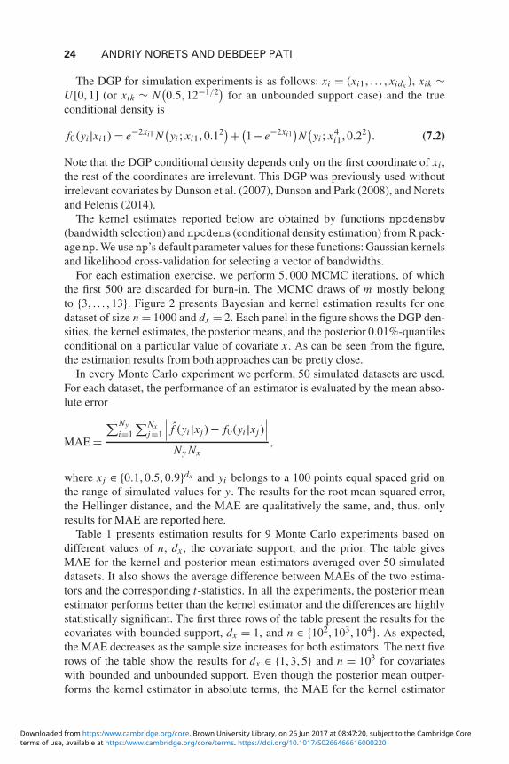
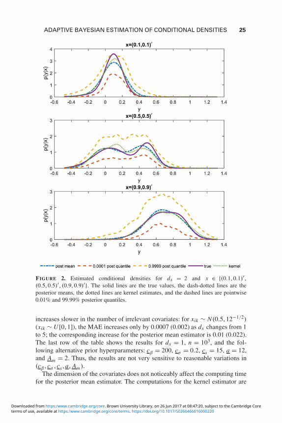
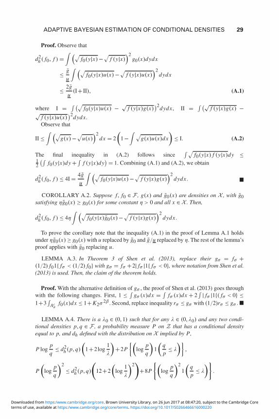