Adrián Bonilla-Petriciolet Gade Pandu Rangaiah … libro...Juan Gabriel Segovia-Hernández and José Enrique Jaime-Leal Department of Chemical Engineering Universidad de Guanajuato,

February 10, 2010 10:16 SPI-B852 9in x 6in b852-ch13

Chapter 13

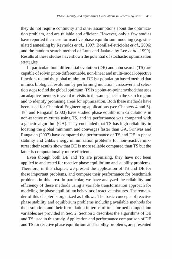
PHASE STABILITY AND EQUILIBRIUMCALCULATIONS IN REACTIVE SYSTEMS USINGDIFFERENTIAL EVOLUTION AND TABU SEARCH

Adrián Bonilla-PetricioletDepartment of Chemical & Biochemical Engineering

Instituto Tecnológico de AguascalientesMéxico, 20256

[email protected]

Gade Pandu RangaiahDepartment of Chemical & Biomolecular EngineeringNational University of Singapore, Singapore, 117576

Juan Gabriel Segovia-Hernándezand José Enrique Jaime-Leal

Department of Chemical EngineeringUniversidad de Guanajuato, Mexico, 36050

1. Introduction

Reactive separations processes (RSPs), where separation and reaction unitsare combined, have received considerable interest from chemical engineersand have been used to develop new technologies for the chemical and

413


414 A. Bonilla-Petriciolet et al.

petrochemical industries. They offer several technological, economic, andoperational advantages over conventional systems (Taylor and Krishna,2000). However, optimal performance of RSPs depends significantly onrelevant process design issues, where the basis for most synthesis and anal-ysis is phase equilibrium behavior. In the design of RSPs, it is often nec-essary to perform numerous phase stability and equilibrium calculations.The goal in phase equilibrium calculations is to determine the numberand identity (composition, quantity and type) of phases existing at equilib-rium for a mixture under specific conditions, while phase stability analysishelps to confirm if the global minimum of Gibbs free energy has beenreached.

There have been many efforts to develop new techniques with the aimof reliably computing phase equilibrium in systems subject to chemicalreactions (Seider and Widagdo, 1996). The existing techniques for thesecalculations can be divided into two main classes: (a) procedures involvingminimization of a suitable objective function, and (b) strategies requiringsolution of nonlinear equations obtained from the stationary conditions ofthat objective function. For the case of phase equilibrium calculations, theobjective function is generally the Gibbs free energy whereas the stabil-ity analysis is performed using the tangent plane distance function. Theavailable strategies can also be classified as either stoichiometric or non-stoichiometric, depending on the formulation of mass balance constraints(Stateva and Wakeham, 1997).

Reactive phase stability and equilibrium problems are non-linear, mul-tivariable and may have multiple solutions. In particular, strong interac-tions among components, phases and reactions increase the complexity ofthese thermodynamic calculations (Xiao et al., 1989; Stateva and Wakeham,1997). Hence, reliable and efficient methods are necessary for solving phaseequilibrium problems of reactive systems. Both deterministic and stochas-tic global solving methods have been proposed for computing chemicaland phase equilibrium simultaneously. The former includes homotopy-continuation and interval methods for non-linear equations, and branch-and-bound optimization strategies. Unfortunately, they generally requirelarge computational effort for multi-component mixtures and, in somecases, problem reformulation is needed (Wakeham and Stateva, 2004).On the other hand, stochastic optimization methods are attractive because


Phase Stability and Equilibrium Calculations in Reactive Systems 415

they do not require continuity and other assumptions about the optimiza-tion problem, and are reliable and efficient. However, only a few studieshave reported their use for reactive phase equilibrium modeling (e.g. sim-ulated annealing by Reynolds et al., 1997; Bonilla-Petriciolet et al., 2006;and the random search method of Luus and Jaakola by Lee et al., 1999).Results of these studies have shown the potential of stochastic optimizationstrategies.

In particular, both differential evolution (DE) and tabu search (TS) arecapable of solving non-differentiable, non-linear and multi-modal objectivefunctions to find the global minimum. DE is a population based method thatmimics biological evolution by performing mutation, crossover and selec-tion steps to find the global optimum. TS is a point-to-point method that usesan adaptive memory to avoid re-visits to the same place in the search regionand to identify promising areas for optimization. Both these methods havebeen used for Chemical Engineering applications (see Chapters 4 and 5).Teh and Rangaiah (2003) have studied phase equilibrium calculations innon-reactive mixtures using TS, and its performance was compared witha genetic algorithm (GA). They concluded that TS has high reliability inlocating the global minimum and converges faster than GA. Srinivas andRangaiah (2007) have compared the performance of TS and DE in phasestability and Gibbs energy minimization problems for non-reactive mix-tures; their results show that DE is more reliable compared than TS but thelatter is computationally more efficient.

Even though both DE and TS are promising, they have not beenapplied to and tested for reactive phase equilibrium and stability problems.Therefore, in this chapter, we present the application of TS and DE forthese important problems, and compare their performance for benchmarkproblems in this area. In particular, we have analyzed the reliability andefficiency of these methods using a variable transformation approach formodeling the phase equilibrium behavior of reactive mixtures. The remain-der of this chapter is organized as follows. The basic concepts of reactivephase stability and equilibrium problems including available methods fortheir solution, and their formulation in terms of transformed compositionvariables are provided in Sec. 2. Section 3 describes the algorithms of DEand TS used in this study. Application and performance comparison of DEand TS for reactive phase equilibrium and stability problems, are presented



in Secs. 4 and 5. Finally, conclusions of this study are provided in the lastsection.

2. Phase Equilibrium and Stability Problemsin Reactive Systems

This section introduces the reader to the basic concepts and descriptionof phase stability and equilibrium problems in reactive systems. Mathe-matically, both the problems can be stated as finding the global minimum,w∗ and f (w∗) of a non-linear function, f (w) of n real decision variables,w = (w1, w2, . . . , wn) subject to w ∈ � where � is the feasible regionsatisfying the governing constraints and bounds on decision variables.

2.1. Description of phase equilibrium problems

In phase equilibrium problems, given components present, temperature andpressure of a system or stream, the main objectives are to correctly establishthe phase number and type, and the distribution of components among thephases at the equilibrium. Classical thermodynamics indicates that mini-mization of the Gibbs free energy is a natural approach for calculating theequilibrium state of a mixture. Most of the available methods for Gibbs freeenergy minimization in reactive mixtures have been proposed during thelast two decades, and they include a variety of problem formulations andnumerical techniques such as local search methods with and without decou-pling strategies (Castillo and Grossmann, 1981; Castier et al., 1989; Xiaoet al., 1989; Gupta et al., 1991; Perez-Cisneros et al., 1997; Stateva andWakeham, 1997), branch-and-bound optimization methods (McDonaldandFloudas, 1996; McKinnon and Mongeau, 1998), algorithms using homo-topy continuation (Jalali and Seader, 1999; Jalali et al., 2008), deterministicmethods based on interval mathematics (Burgos-Solorzano et al., 2004) andstochastic optimization methods (Reynolds et al., 1997; Lee et al., 1999;Bonilla-Petriciolet et al., 2006; Bonilla-Petriciolet et al., 2008).

In general, there are several challenges in computing the global min-imum of the Gibbs free energy function. First, the number and typesof phases, at which this thermodynamic function achieves the globalminimum, are usually not known a priori. Hence, several equilibriumcalculations must be performed using different phase configurations



(adding or removing phases) to identify the stable equilibrium state. More-over, for a fixed number of phases and components, Gibbs free energyfunction may have a local minimum value very comparable to the globalminimum value, which makes it challenging to find the global minimum(Srinivas and Rangaiah, 2007). The poor conditioning of the Hessian matrixof the free energy for mixtures near phase boundaries (such as bubble, dewand critical points) may lead to failure of solving strategies (Seider andWidagdo, 1996). Trivial solutions, which satisfy the necessary equilibriumconditions and the mass constraints in the system, also exist but they arelocal optima of Gibbs free energy. Consequently, many strategies in theliterature are local methods, depend on initialization and may converge tounstable solutions. These limitations have prompted the development ofreliable algorithms for the global minimization of Gibbs free energy.

Many available methods for phase equilibrium problems in reactive sys-tems, use conventional composition variables (mole numbers or fractions)as decision variables. A few studies have considered variable transformationapproaches with the goal of developing a simpler thermodynamic frame-work for modeling reactive systems (e.g. Ung and Doherty, 1995b; Perez-Cisneros et al., 1997). These approaches, in combination with appropriatemethods such as stochastic optimization strategies, can be used to developreliable techniques for computing phase equilibrium of reactive systems.Therefore, in this chapter we have used a suitable transformation schemeto formulate phase equilibrium and stability problems involving chemicalreactions.

2.1.1. Formulation of the optimization problem

In a reactive mixture with c components and r independent chemical reac-tions (with r < c) that splits into π phases, the Gibbs free energy functioncan be written as

�g =π∑

j=1

c−r∑i=1

ni, j

(�µi, j

RT

), (1)

where �g is the dimensionless transformed molar Gibbs free energy ofmixing (Ung and Doherty, 1995b), ni, j is the transformed mole number of



component i in phase j and�µi, j

RT is the chemical potential of component iin phase j . The transformed mole number and other transformed variablesare defined below. Further, the following mass balances must be satisfied:

ni,F −π∑

j=1

ni, j = 0 for i = 1, . . . , c − r, (2)

where ni,F is the transformed mole number of component i in the feed (orinitial system).

The Gibbs free energy minimization problem is to minimize Eq. (1) withrespect to ni, j (for i = 1, . . . , c − r and j = 1, . . . , π) subject to Eq. (2).Note that the chemical potentials in Eq. (1) are functions of transformedcomposition variables, which depend on the thermodynamic model usedfor predicting behavior of each phase.

Transformed mole numbers ni , for a system of c components (includingboth reacting and inert species) subject to r independent chemical reactions,are defined by selecting a set of r reference components (Ung and Doherty,1995a; 1995b) as:

ni = ni − vi N−1nref , (3)

where ni is the number of moles of component i , nref is a column vectorof dimension r of the moles of each of the reference components, vi isthe row vector of stoichiometric coefficients of component i for each ofthe r reactions, and N is an invertible and square matrix formed from thestoichiometric coefficients of the reference components in the r reactions.Note that vi,k < 0 for reactants, vi,k > 0 for products, and vi,k = 0 for inertcomponents.

Consequently, the total amount of transformed moles nT is

nT =c−r∑i=1

ni = nT − vTOTN−1nref . (4)

Here, nT is the total number of moles present at any instant of time, and vTOT

is a row vector where each element corresponds to the sum of stoichiometriccoefficients for all components that participate in each of the r reactions.



Dividing ni by nT , the transformed mole fractions Xi are obtained:

Xi = ni

nT= xi − vi N−1x ref

1 − vTOTN−1xrefi = 1, . . . , c − r, (5)

where xi is the mole fraction of component i and x ref is the column vectorof r reference component mole fractions. Due to mass balance restrictions,the sum of all transformed mole fractions must equal unity, or

∑c−ri=1 Xi = 1

(Ung and Doherty, 1995a; 1995b).The transformed composition variables (ni and Xi ) depend only on the

initial composition of each independent chemical species and take the samevalue before, during and after reaction (Ung and Doherty, 1995a; 1995b).They also restrict the solution space to the compositions that satisfy stoi-chiometry requirements and reduce the dimension of the composition spaceby the number of independent reactions. The transformed variables allowall of the procedures used to compute phase equilibrium/stability of non-reactive mixtures to be extended to systems with chemical reactions (Ungand Doherty, 1995a; 1995b). They (n and X) in reactive systems play thesame role as the usual composition variables (n and x) in non-reactive mix-tures. However, transformed variables can be negative or positive dependingon the reference components, number and type of reactions.

In Appendix A, we use a simple reactive mixture to illustrate the corre-spondence between the transformed composition variables (n and X) andthe usual composition variables (n and x) at equilibrium, and how to calcu-late the previous ones by specifying the transformed variables and applyingthe chemical equilibrium constraints:

Keq,k =c∏

i=1

avi,ki , k = 1, . . . , r, (6)

where Keq,k is the equilibrium constant for reaction k and ai is the activityof component i . The formulation of phase equilibrium problem for thissimple reactive mixture is also shown in this appendix.

For a reactive mixture, minimizing Gibbs free energy with respect to n isequivalent to minimizing the transformed Gibbs free energy with respect ton (Ung and Doherty, 1995b). The Gibbs free energy minimization problemhas equality constraints (Eq. (2)). To perform an unconstrained minimiza-tion of free energy, we can use a set of new variables instead of transformed



composition variables as decision variables. The introduction of these vari-ables automatically satisfies the equality constraints (Eq. (2)) and reducesproblem dimensionality further. Assuming that all transformed mole frac-tions have values in the range Xi, j ∈ (0, 1), real variables λi, j ∈ [0, 1] aredefined and employed as decision variables using the following expressions:

ni,1 = λi,1ni,F for i = 1, . . . , c − r, (7)

ni, j = λi, j

ni,F −

j∑m=1

ni,m

for i = 1, . . . , c − r and

j = 2, . . . , π − 1, (8)

ni,π = ni,F −π−1∑m=1

ni,m for i = 1, . . . , c − r, (9)

where ni,F = ni,F − vi N−1nref,F , nT,F = nT,F − vTOT N−1nref,F =∑c−ri=1 ni,F , nT,F = ∑c

i=1 ni,F and ni,F is the number of moles of compo-nent i in the feed. Note that Zi = ni,F/nT,F .

Using the formulation in Eqs. (7) to (9), all trial compositions will satisfythe mass balances (Eq. (2)), the optimization problem will have only boundson decision variables and no other constraints, allowing the easy applicationof stochastic global optimization strategies. Recently, Bonilla-Petricioletet al. (2008) have reported the application of simulated annealing (SA) forthe minimization of the transformed Gibbs free energy minimization usingthe above formulation, and concluded that SA is reliable for this purpose.However, this method required significant computational effort. The studyof Bonilla-Petriciolet et al. (2008) is the first attempt to apply a stochasticglobal method to the optimization of Gibbs free energy using transformedcomposition variables, and it is desirable to test other stochastic methods forthis application. Hence, in this chapter, DE and TS are tested and comparedfor phase equilibrium calculations of reactive systems via Gibbs free energyminimization and transformed composition variables.

2.2. Description of phase stability problem

Phase stability analysis allows identification of the thermodynamic statethat corresponds to the global minimum of the Gibbs free energy



(i.e. globally stable equilibrium). A phase at a given temperature, pres-sure and composition, is stable if and only if the Gibbs free energy surfaceis at no point below the tangent plane to the surface at the given composi-tion (Baker et al., 1982; Michelsen, 1982). This statement is a necessaryand sufficient condition for global stability. Generally, stability analysis inreactive systems is performed by the minimization of the distance betweenthe Gibbs free energy surface and the tangent plane to the surface at thegiven composition (known as the tangent plane distance function, TPDF)with respect to all possible phase compositions, using mole numbers orfractions as decision variables. Non-negativity of the global minimum ofthis function implies that the given phase is stable. Note that stability calcu-lations in reactive mixtures using TPDF must be performed only for phasesthat are chemically equilibrated (Michelsen, 1982; Castier et al., 1989). Thisis because, in reactive systems, the total number of moles (nT ) present atany instant of time may not remain constant as the reactions proceed. Thus,it is not meaningful to directly minimize TPDF to study stability in reac-tive mixtures, and the proposed methods execute a chemical equilibrationprocedure before phase stability calculations.

Similar to the phase equilibrium calculations, phase stability anal-ysis in reactive systems is a challenging global optimization problembecause the objective function is multivariable, non-convex and highlynon-linear. Many optimization methods have been tried for stability cal-culations in reactive systems using the classical tangent plane criterion(e.g. Gupta et al., 1991; Stateva and Wakeham, 1997; Jalali and Seader,1999; Jalali et al., 2008). Traditional approaches, which generally utilizedifferent initial estimates and local search methods, may converge to alocal or trivial solution based on the initial guess. Several determinis-tic global optimization methods have also been tested for phase stabil-ity analysis in reactive systems; these include branch-and-bound methods(McDonald and Floudas, 1996; McKinnon and Mongeau, 1998), homotopycontinuation algorithms (Jalali-Farahaniand Seader, 2000) and the interval-Newton/general-bisection approach (Burgos-Solorzano et al., 2004).

Since the tangent plane criterion is also applicable to chemicallyequilibrated phases, any method proposed for stability calculations in non-reactive systems can be extended to reactive mixtures. Hence, stochas-tic optimization methods such as SA, GA, TS and DE can be used for



this purpose (Rangaiah, 2001; Teh and Rangaiah, 2003; Bonilla-Petricioletet al., 2006; Srinivas and Rangaiah, 2007). Further, it is possible to refor-mulate the tangent plane criterion in terms of transformed compositionvariables. This modified stability criterion, adopted for the present study,and its advantages are described below.

2.2.1. Formulation of the optimization problem

Based on the transformed variables of Ung and Doherty (1995a, 1995b),Wasylkiewicz and Ung (2000) introduced the reactive tangent plane dis-tance function (RTPDF) for multi-component and multi-reaction systems,which is defined as

RTPDF =c−r∑i=1

Xi

(�µi

RT

∣∣∣∣X

− �µi

RT

∣∣∣∣Z

), (10)

where �µiRT

∣∣X and �µi

RT

∣∣Z are the chemical potentials of component i calcu-

lated at the transformed mole fractions X and Z , respectively. The RTPDFrepresents the vertical displacement from the tangent plane at the givencomposition Z , to the transformed molar Gibbs free energy surface at thecomposition X.The necessary and sufficient condition for global phase sta-bility is given by RTPDF ≥ 0.0 for any X in the whole transformed com-position space. There is at least one solution for RTPDF (= 0.0) at thetrivial stationary point X = Z . For a stable phase, this must be the globalminimum of RTPDF.

RTPDF and its stationary points for arbitrary stable and unstable reactivemixtures are illustrated in Fig. 1. In the upper-left plot of this figure, thetangent to the transformed Gibbs free energy at Z lies below this freeenergy surface throughout the transformed composition space, and, as aconsequence, a single phase with the transformed composition Z is stable(i.e. the global minimum of RTPDF is 0.0 at Z , as shown in the lower-leftplot). In another case shown in the upper-right plot, the tangent at Z crossesthe Gibbs free energy surface at several points; therefore, a phase with thistransformed composition is unstable. This unstable mixture shows severalstationary points for RTPDF (see the lower-right plot).

The minimization problem for phase stability via tangent plane crite-rion is to minimize Eq. (10) with respect to Xi (for i = 1, . . . , c − r )



-0.16

-0.12

-0.08

-0.04

0.00

0.0 0.2 0.4 0.6 0.8 1.0

Stable reactive mixture with transformed composition Z

-0.16

-0.12

-0.08

-0.04

0.00

0.0 0.2 0.4 0.6 0.8 1.0

Unstable reactive mixture with transformed composition Z

0.00

0.10

0.20

0.30

0.40

0.50

0.0 0.2 0.4 0.6 0.8 1.0

Global minimumX = Z

-0.05

0.00

0.05

0.10

0.15

0.20

0.0 0.2 0.4 0.6 0.8 1.0

Stationary points

Global minimum

X1

g∆R

TP

DF

0.2 0.3

Trivial Solution X= Z

Figure 1. Gibbs free energy of mixing,�g and RTPDF for a reactive mixture wherec − r = 2, illustrating the transformed mole fraction Z of stable and unstable reactivemixtures, and their corresponding stationary points and global minimum of RTPDF. Trans-formed mole fraction of one component (X1) is shown on the x-axis and that of the secondcomponent is X2 = 1.0 − X1.

subject to∑c−r

i=1 Xi = 1. Instead of λ’s used as decision variables in phaseequilibrium problems to automatically satisfy the equality constraints, analternate strategy is employed in phase stability problems. Here, (c − r)

decision variables, each in the range 0.0 to 1.0, are generated and then nor-malized so that their sum is equal to unity. The resulting variable valuesare used for calculating the objective, RTPDF. This strategy will not reducethe number of decision variables but this is not important since number ofvariables in phase stability problems is less than that in phase equilibriumproblems. Note that the chemical potentials in Eq. (10) are functions of Xi ,which depend on the thermodynamic model used for predicting the phasebehavior. For illustration, phase stability problem for the simple case of anideal ternary mixture is formulated in Appendix A.

The RTPDF offers two main advantages over the classical TPDFin the stability analysis of reactive systems (Ung and Doherty, 1995b;



Wasylkiewicz and Ung, 2000). First, given the initial composition of thereactive mixture, one can perform the stability test directly using theRTPDF, in contrast to the classical TPDF, where a preliminary chemi-cal equilibration procedure is required. In fact, this equilibration procedureis implicit if the transformed variables are used. Another advantage ofthis approach is the significant reduction of problem dimensionality formulti-reaction systems.

A few studies have dealt with the global solution of RTPDF.Wasylkiewicz and Ung (2000) applied the homotopy continuation approachto locate all stationary points of RTPDF. Bonilla-Petriciolet et al. (2006)reported the application of stochastic optimization methods: SA, very fastSA, modified direct search SA and stochastic differential equations, for theglobal minimization of RTPDF. Among the methods tested, they found thatSA is a reliable strategy for stability calculations in reactive mixtures; butits computational effort is very high for multi-component systems. Thesestudies are the first attempts for the global solution of RTPDF. Hence, effi-cacy of TS and DE for the global minimization of RTPDF is studied in thischapter.

3. DE and TS, and Parameter Tuning

Introduction to and description of DE and TS are provided in earlier chap-ters. In the present study, FORTRAN codes developed by Teh and Rangaiah(2003), and Srinivas and Rangaiah (2007) for TS and DE algorithms, respec-tively, were used. Both methods have been implemented in combinationwith a local optimization technique for finding the global minimum accu-rately and efficiently. Figure 2 shows the flowchart of these hybrid algo-rithms; see Teh and Rangaiah (2003) and Srinivas and Rangaiah (2007)for the description of these algorithms. For local optimization, we haveused a fast convergent quasi-Newton method implemented in the subrou-tine DBCONF from IMSL library. This subroutine calculates the gradientvia finite differences and approximates the Hessian matrix (consisting ofsecond derivatives of the objective function) according to BFGS formula. Inbrief, a quasi-Newton method is a modification of Newton method withoutthe need for second derivatives of the objective function. For more detailson this local strategy, see the optimization book by Dennis and Schnabel(1983). The default values of DBCONF parameters in the IMSL library



Start

Set values for DE parameters

Generate the initial population andevaluate the objective function.

Evaluate the individuals and selectthe best one.

Set Generation = 1

Mutation

Crossover

Selection

Is the stopping criterion satisfied?

Local optimization using quasi-Newton method.

Stop

Generation =Generation + 1

Yes

No

Start

Set values for DE parameters

Generate the initial population andevaluate the objective function.

Evaluate the individuals and selectthe best one.

Set Generation = 1

Mutation

Crossover

Selection



Stop

Generation =Generation + 1Generation =Generation + 1

Yes

No

Start

Set values for TS parameters

Generate the initial population and evaluate the objective function.

Select the best point as the currentcentroid, s and fill it into promisinglist. Fill rest of the points into tabulist.

Set Iteration = 1



Stop

Iteration = Iteration + 1

Yes

No

Generate n-neighbors in hyper-rectangles with centroid, s.

Reject those generated neighborswhich are close to those points inthe tabu and promising lists.

a) Evaluate the objective functionat the remaining neighbors and set the best neighbor as the new centroid, s.

b) Update promising and tabulists.

Identify the most promising point.

Start

Set values for TS parameters

Generate the initial population and evaluate the objective function.

Select the best point as the currentcentroid, s and fill it into promisinglist. Fill rest of the points into tabulist.

Set Iteration = 1



Stop

Iteration = Iteration + 1Iteration = Iteration + 1

Yes

No

Generate n-neighbors in hyper-rectangles with centroid, s.

Reject those generated neighborswhich are close to those points inthe tabu and promising lists.

a) Evaluate the objective functionat the remaining neighbors and set the best neighbor as the new centroid, s.

b) Update promising and tabulists.

Identify the most promising point.

Figure 2. Flowcharts of DE (on the left) and TS (on the right).

were used in our calculations. The procedure used for tuning of DE and TSparameters is described below.

3.1. Tuning of TS and DE parameters usingperformance profiles

Like any stochastic method, TS and DE have a number of parameters thatneed to be heuristically tuned for any desired application. This tuning is a



key step in the application and evaluation of a stochastic method, wherea proper selection of its parameters is essential to achieve the best reli-ability and efficiency of the method. Parameter tuning is generally per-formed using benchmark problems and determining the average valuesof specific performance metrics. However, using this approach, a smallnumber of the most difficult problems may tend to dominate the resultsfor performance metrics and, as a consequence, lead to incorrect conclu-sions about the algorithm performance (Dolan and More, 2002). To addressthis shortcoming, we have employed the performance profile (PP) reportedby Dolan and More (2002) to tune the parameters of both TS and DEmethods.

Dolan and More (2002) introduced PP as an alternative tool for evaluat-ing and comparing the performance of optimization software. In particular,PP has been proposed to compactly and comprehensively represent thedata collected from a set of solvers for a specified performance metric. Forinstance, number of function evaluations (NFE) or computing time (CPUt)can be considered performance metrics for solver comparison. The PP plotallows visualization of the expected performance differences among sev-eral solvers and to compare the quality of their solutions by eliminating thebias of failures obtained in a small number of problems.

To introduce PP, consider ns solvers (i.e. optimization methods) to betested over a set � of n p problems. For each problem p and solver s, theperformance metric tps must be defined. In our study, reliability of stochasticmethods in accurately finding the global optimum of the objective functionis considered as the principal goal, and hence the performance metric isdefined as

tps = fcalc − f ∗, (11)

where f ∗ is the known global optimum of the objective function and fcalc

is the mean value of that objective function calculated by the stochasticmethod over several runs. In this study, fcalc is calculated from 100 runsto solve each test problem by each solver; note that each run is differ-ent because of random number seed used and the stochastic nature of themethod. So, the focus is on the average performance of stochastic methods,which is desirable (Ali et al., 2005).



For the performance metric of interest, the performance ratio, rps is usedto compare the performance on problem p by solver s with the best perfor-mance by any solver on this problem. This performance ratio is given by

rps = tps

min{tps : 1 ≤ s ≤ ns} . (12)

The value of rps is 1 for the solver s that performs the best on a specificproblem p. For example, if rps = 2, the performance metric of solver son problem p is twice the best value found by another solver on the sameproblem p.

To obtain an overall assessment of the performance of solver s on n p

problems, the following cumulative function for rps is used:

ρs(ς) = 1

n psize {p ∈ � : rps ≤ ς}, (13)

where ρs(ς) is the fraction of the total number of problems, for whichsolver s has a performance ratio rps within a factor ς ∈ (1,∞) of the bestpossible ratio. The PP of a solver is a plot of ρs(ς) versus ς; it is a non-decreasing, piece-wise constant function, continuous from the right at eachof the breakpoints (Dolan and More, 2002).

Note that 1.0 − ρs(ς) is the fraction of problems that solver s failed tosolve within a factor ς of the best method. This implies that, if the set ofn p problems is reasonably large and representative of circumstances thatare likely to occur in the desired application, then solvers with larger ρs(ς)

are better. If the objective is to identify the best solver, it is only necessaryto compare the values of ρs(1) for all solvers and to select the highest one,which is the probability that a specific solver will “win” over the rest ofsolvers used. For the performance metric in Eq. (11), the PP plot compareshow accurately the stochastic methods can find the global optimum valuerelative to one another, and so the term “win” refers to the stochastic methodthat provides the most accurate value of the global optimum in reactivephase stability and equilibrium problems. We have calculated several PPs,and results are used for tuning TS and DE parameters for reactive phasestability and equilibrium calculations.

Parameters tuned in this study are: (a) DE: amplification factor (A),crossover constant (CR), population size (NP), maximum number of



generations (Genmax), and maximum number of generations withoutimprovement in the best function value (Scmax); and (b) TS: tabu list size(Nt ), promising list size (N p), tabu radius (εt ), promising radius (εp),length of the hyper-rectangle (hn), initial population size (NPinit), and max-imum number of iterations (Itermax) and Scmax. Note that Genmax, Itermax

and Scmax are the stopping criteria for DE and TS. The parameter tuning wasperformed using the stochastic methods without a local search algorithm.This procedure was carried out by varying one parameter at a time, whilethe remaining parameters were fixed at their nominal values. The testedand nominal values for each strategy are given in Table 1. Some algorithmparameters were associated to nvar (i.e. number of decision variables), and

Table 1. Parameters tested for tuning of TS and DE for the global minimization of �g andRTPDF.

Method Parameter Tested valuesa Nominal value

DE Amplification factor A 0.3, 0.5, 0.7 0.5Crossover constant CR 0.1, 0.5, 0.9 0.1Population size NP 5nvar , 10nvar ,

25nvar , 50nvar

10nvar

Maximum number of generationsGenmax

50, 100, 200 50

Maximum number of generationswithout improvement in the bestfunction value Scmax

6nvar , 12nvar 12nvar

TS Tabu list size Nt 5, 10, 20 10Promising list size Np 5, 10, 20 10Tabu radius εt 0.005, 0.01, 0.02 0.01Promising radius εp 0.005, 0.01, 0.02 0.01Length of the hyper-rectangle hn 0.25, 0.5, 0.75 0.5Initial population size NPinit 10nvar , 20nvar ,

30nvar

20nvar

Maximum number of iterationsItermax

25nvar , 50nvar ,100nvar

50nvar

Maximum number of iterationswithout improvement in the bestfunction value Scmax

2nvar , 6nvar ,12nvar

6nvar

Number of neighbors, Nneighsubject to a minimum of 10 anda maximum of 30.

2nvar 2nvar

anvar is the number of decision variables in the optimization problem.



all values tested were chosen based on the results reported by Teh andRangaiah (2003) and Srinivas and Rangaiah (2007).

For comparing the algorithm efficiency, NFE and CPUt were used asmeasures of computational effort. All calculations were performed on theIntel Pentium M 1.73 GHz processor with 504 MB of RAM. This com-puter performs 254 million floating point operations per second (MFlops)for the LINPACK benchmark program (available at http://www.netlib.org/;accessed in July, 2008) for a matrix of order 500.

4. Phase Equilibrium Calculations in Reactive Systemsusing DE and TS

4.1. Benchmark problems for parameter tuning

For parameter tuning, we have considered three reactive systems thatare benchmarks in the studies on RSPs; they are: (a) the reaction forbutyl acetate production at 298.15 K and 1 atm, (b) methyl tert-butyl ether(MTBE) reaction system with inert at 10 atm and 373.15 K, and (c) thereactive system for tert-amyl methyl ether (TAME) synthesis at 335 K and1.5 atm. Thermodynamic models, parameters and transformed variablesfor these reactive systems are reported in Table 2, and Tables B1 - B3 ofAppendix B. For variable transformation, the reference components arearbitrarily selected, and we have c − r = 3 transformed composition vari-ables for all systems.

In the three problems, the number of phases existing at the equilibriumis assumed to be known a priori, but the phase type (vapor or liquid) isunknown. Bisection method is used to perform the composition transfor-mation: X → x (see Appendix A), for objective function evaluation. Notethat x obtained from this transformation satisfy the stoichiometry require-ments and are chemically equilibrated. Further, the chemical potentials in�g and RTPDF (Eqs. 1 and 10) are given by:

�µi

RT= µi − µ0

i

RT= ln

(xi ϕi

ϕi

)= ln(xiγi ), (14)

where µ0i is the chemical potential of pure component i , ϕi is the fugacity

coefficient of component i in the mixture, ϕi is the fugacity coefficient ofpure component, γi is the activity coefficient of component i in the mixture,and xi is the mole fraction of component i in the mixture.



Tabl

e2.

Det

ails

ofth

ese

lect

edre

activ

em

ixtu

res

for

para

met

ertu

ning

ofT

San

dD

Efo

rre

activ

eph

ase

equi

libri

umpr

oble

ms.

Mix

ture

Pha

ses

and

ther

mod

ynam

icm

odel

s(s

eeA

ppen

dix

Bfo

rpa

ram

eter

valu

es)

Tra

nsfo

rmed

mol

efr

acti

ons

A1

+A

2↔

A3

+A

4(1

)A

ceti

cA

cid

(2)

n-B

utan

ol(3

)W

ater

(4)

n-B

utyl

acet

ate

Liq

uid-

liqu

ideq

uili

briu

m,U

NIQ

UA

Cm

odel

.ln

Keq

,1=

450

T+

0.8

whe

reT

isin

K.

Mod

elpa

ram

eter

sar

eta

ken

from

Was

ylki

ewic

zan

dU

ng(2

000)

.

X1

=x 1

+x 4

X2

=x 2

+x 4

X3

=x 3

−x 4

=1

−X

1−

X2

Ref

eren

ceco

mpo

nent

:A

4

A1

+A

2↔

A3,

and

A4

asan

iner

t(1

)Is

obut

ene

(2)

Met

hano

l(3

)M

ethy

lter

-but

ylet

her

(4)

n-B

utan

e

Vap

or-l

iqui

deq

uili

briu

m,W

ilso

nm

odel

and

idea

lgas

.�

Go rx

s/R

=−4

205.

05+

10.0

982T

−0.

2667

Tln

T

lnK

eq,1

=−�

G0 rx

sR

Tw

here

Tis

inK

.M

odel

para

met

ers

are

take

nfr

omU

ngan

dD

oher

ty(1

995a

).

X1

=x 1

+x3

1+x 3

X2

=x 2

+x3

1+x 3

X4

=x 4

1+x 3

=1

−X

1−

X2

Ref

eren

ceco

mpo

nent

:A

3

A1

+A

2+

2A

3↔

2A

4(1

)2-

Met

hyl-

1-bu

tene

(2)

2-M

ethy

l-2-

bute

ne(3

)M

etha

nol

(4)

Tert

-am

ylm

ethy

leth

er

Vap

or-l

iqui

deq

uili

briu

m,W

ilso

nm

odel

and

idea

lgas

.K

eq,1

=1.

057

·10−

04e42

73.5

/T

whe

reT

isin

K.

Mod

elpa

ram

eter

sar

eta

ken

from

Bon

illa

-Pet

rici

olet

etal

.(20

08).

X1

=x 1

+0.5

x 41+

x 4X

2=

x 2+0

.5x 4

1+x 4

X3

=x 3

+x4

1+x 4

=1

−X

1−

X2

Ref

eren

ceco

mpo

nent

:A

4



(a)

0

0.2

0.4

0.6

0.8

1

0 0.2 0.4 0.6 0.8 1

2X

1X(b)

0

0.2

0.4

0.6

0.8

1

0 0.2 0.4 0.6 0.8 1

2X

1X(c)

0

0.2

0.4

0.6

0.8

1

0 0.2 0.4 0.6 0.8 11X

2X

Figure 3. Transformed feed (◦) and tie-lines (•) used for parameter tuning of TS and DEin reactive phase equilibrium problems. Reactive systems are: (a) acetic acid + n-butanol↔ water + n-butyl acetate at 298.15 K and 1 atm, (b) isobutene + methanol ↔ methyltert-butyl ether with n-butane as an inert at 10 atm and 373.15 K, and (c) 2-methyl-1-butene+ 2-methyl-2-butene + 2 methanol ↔ 2 tert-amyl methyl ether at 335 K and 1.5 atm.

Feed compositions and tie-lines used to tune the parameters of TS andDE are shown in Fig. 3. We have utilized n p = 48 different feeds, selectedfrom the three reactive mixtures, to calculate PPs. The objective functionhas at least one local minimum, which corresponds to a trivial solution



(Zi = Xi in phase stability and Zi = Xi,1 = · · · = Xi,π in equilibriumcalculations), for all tested conditions. Note that different models are usedin the calculation of thermodynamic properties for different phases (vaporand liquid) of reactive systems (b) and (c). The use of multiple thermody-namic models increases the complexity of phase stability and equilibriumcalculations (Xu et al., 2005); since there will be different �g functionsfor different types of phases, evaluation of any trial composition must bedone on the surface with the lowest value of transformed Gibbs free energy.Thus, the procedure of variable transformation is performed for each modelat specified X and its corresponding �g is evaluated. The model having thelowest value of transformed Gibbs free energy is then used for evaluatingthe objective function. Finally, the selected conditions involve feed com-positions near phase boundaries, which are generally challenging for anyalgorithm. So, the tested conditions are appropriate for tuning the parame-ters of TS and DE.

In the three reactive systems considered for parameter tuning, c = 4 andr = 1 (see Table 2). Hence, there are three decision variables, λi,1 ∈ (0, 1)

in the Gibbs energy minimization for phase equilibrium calculations. Inthe problems to test stability of the feed, depending upon the permissiblevalues for X , we have considered different transformed variables and theequality constraint

∑c−ri=1 Xi = 1. For the reactive system (a), RTPDF is

minimized with respect to X1, X2 ∈ (0, 1) only, and X3 = 1−X1−X2. Forphase stability calculations in reactive systems (b) and (c), three transformedfractions Xi ∈ (0, 1) are used as decision variables, after their normalizationto unity: Xi = Xi/

∑c−ri=1 Xi where Xi is the normalized transformed mole

fraction of component i .

4.2. Results of parameter tuning

Table 3 shows the performance summary for tuning the parameters of TSand DE; in this table, we report ρs(1), NFE and CPUt obtained in the globalminimization of RTPDF and �g. Here, NFE and CPUt are the mean of 100runs for 48 feeds, and the range given for NFE and CPUt in each rowof Table 3 is for the three problems solved. Depending on the parametervalues, NFE varied from 390 to 7626 for stability calculations by DE, whileit varied from 105 to 801 for stability calculations by TS; this computational



Tabl

e3.

Res

ults

for

para

met

ertu

ning

ofT

San

dD

Efo

rth

egl

obal

min

imiz

atio

nof

�g

and

RT

PD

F.

Para

met

ertu

ning

Pro

babi

lity

,ρs(

1)fo

rN

FE

for

CP

Ut(

s)fo

r

Met

hod

Para

met

erV

alue

aR

TP

DF

�g

RT

PD

F�

gR

TP

DF

�g

DE

A0.

30.

542

0.62

576

9–15

2814

71–1

524

0.17

–0.5

30.

43–0

.93

0.5

0.20

80.

292

779–

1524

1457

–152

30.

18–0

.53

0.44

–0.9

40.

70.

250

0.08

377

2–15

2714

62–1

515

0.17

–0.5

30.

44–0

.94

CR

0.1

0.0

0.0

779–

1524

1457

–152

30.

18–0

.53

0.44

–0.9

40.

50.

042

0.02

196

8–15

3015

13–1

530

0.16

–0.5

30.

44–0

.94

0.9

0.95

80.

979

1020

–153

015

11–1

530

0.16

–0.5

10.

45–0

.95

NP

5nva

r0.

00.

039

6–76

273

0–75

80.

09–0

.28

0.21

–0.4

810

n var

0.0

0.0

779–

1524

1457

–152

30.

18–0

.53

0.44

–0.9

425

n var

0.0

0.0

1830

–381

536

66–3

804

0.28

–1.2

81.

07–2

.34

50n v

ar1.

01.

036

72–7

626

7239

–757

90.

69–2

.54

2.01

–4.6

9

Gen

max

500.

021

0.0

779–

1524

1457

–152

30.

18–0

.53

0.44

–0.9

410

00.

292

0.39

680

5–28

4520

58–2

602

0.22

–0.8

50.

69–1

.58

200

0.68

80.

604

825–

5006

2160

–339

60.

26–1

.17

0.71

–1.9

6

Scm

ax6n

var

0.0

0.0

390–

1291

1015

–122

00.

09–0

.48

0.42

–0.7

212

n var

1.0

1.0

779–

1524

1457

–152

30.

18–0

.53

0.44

–0.9

4

(Con

tinu

ed)



Tabl

e3.

(Con

tinu

ed)

Para

met

ertu

ning

Pro

babi

lity

,ρs(

1)fo

rN

FE

for

CP

Ut(

s)fo

r

Met

hod

Para

met

erV

alue

aR

TP

DF

�g

RT

PD

F�

gR

TP

DF

�g

TS

Nt=

Np

50.

771

0.81

320

3–63

648

4–68

00.

03–0

.16

0.15

–0.4

110

0.08

30.

083

194–

455

385–

521

0.04

–0.1

30.

11–0

.30

200.

146

0.10

419

3–44

239

3–52

20.

03–0

.12

0.14

–0.2

5

ε t=

εp

0.00

50.

875

0.93

822

6–49

840

8–68

10.

03–0

.14

0.14

–0.3

50.

010.

125

0.04

219

4–45

538

5–52

10.

04–0

.13

0.11

–0.3

00.

020.

00.

021

172–

418

347–

408

0.03

–0.1

20.

11–0

.26

hn

0.25

0.22

90.

333

182–

444

369–

511

0.03

–0.1

30.

10–0

.30

0.5

0.39

60.

375

194–

455

385–

521

0.04

–0.1

30.

11–0

.30

0.75

0.37

50.

292

208–

456

390–

543

0.02

–0.1

20.

11–0

.29

NP

init

10n v

ar0.

250

0.25

018

3–43

036

1–51

90.

03–0

.12

0.09

–0.2

720

n var

0.43

80.

458

194–

455

385–

521

0.04

–0.1

30.

11–0

.30

30n v

ar0.

313

0.29

221

4–46

241

7–54

10.

03–0

.12

0.11

–0.3

0

Iter

max

25n v

ar,

0.33

30.

229

192–

443

375–

487

0.03

–0.1

20.

08–0

.30

50n v

ar0.

396

0.41

719

4–45

538

5–52

10.

04–0

.13

0.11

–0.3

010

0nva

r0.

271

0.37

519

6–45

939

3–53

20.

03–0

.11

0.12

–0.4

2

Scm

ax2n

var

0.0

0.0

105–

223

177–

241

0.01

–0.0

60.

07–0

.11

6nva

r0.

063

0.0

194–

455

385–

521

0.04

–0.1

30.

11–0

.30

12n v

ar0.

938

1.0

296–

801

656–

849

0.05

–0.2

40.

13–0

.53

aR

emai

ning

para

met

ers

wer

efi

xed

atno

min

alva

lues

,see

Tabl

e1.



effort corresponds to 0.09–2.54 s of CPUt for DE, and 0.01–0.24 s for TS(see Table 3). For Gibbs free energy minimization, NFE varied from 730to 7579 (0.21–4.69 s) for DE, and from 177 to 849 (0.07–0.53 s) for TS,depending on the parameter values.

Since we are only interested in the optimal values of parameters of TSand DE that find the best solution of all tested conditions, only ρs(1) isgiven in Table 3 and not the PPs. However, for illustrative purposes, severalPPs obtained for TS and DE are shown in Figs. 4 and 5, which displays thefraction of phase stability and equilibrium problems solved by TS and DEwith different parameter values, within a factor ς of the best found solution.These PPs show the effect of a parameter on the relative performance of TSand DE, and enable to find the optimal values of parameters. The results inTable 3 show that algorithm reliability increases with NP, Genmax, Itermax

and Scmax, but at the expense of computational effort. The PPs also showthat optimal values of A = 0.3 and CR = 0.9 for DE agree with those

0

0.1

0.2

0.3

0.4

0.5

0.6

0.7

0.8

0.9

1

1 2 3 4 5 6 7 8 9 10

0.5

0.30.7

A

0

0.1

0.2

0.3

0.4

0.5

0.6

0.7

0.8

0.9

1

1 2 3 4 5 6 7 8 9 10

0.5

0.3

0.7

A

0

0.1

0.2

0.3

0.4

0.5

0.6

0.7

0.8

0.9

1

1 2 3 4 5 6 7 8 9 10

0.1

0.5

0.9

CR

0

0.1

0.2

0.3

0.4

0.5

0.6

0.7

0.8

0.9

1

1 2 3 4 5 6 7 8 9 10

0.1

0.5

0.9

CR

ζ

ρs

Figure 4. Performance profiles for algorithm parameters of DE in reactive phase stability(RTPDF: plots in the left column) and equilibrium calculations (�g: plots in the rightcolumn).



ρs

0

0.1

0.2

0.3

0.4

0.5

0.6

0.7

0.8

0.9

1

1 2 3 4 5 6 7 8 9 10

10

5

20

N t = N p

0

0.1

0.2

0.3

0.4

0.5

0.6

0.7

0.8

0.9

1

1 2 3 4 5 6 7 8 9 10

10

5

20

N t = N p

0

0.1

0.2

0.3

0.4

0.5

0.6

0.7

0.8

0.9

1

1 2 3 4 5 6 7 8 9 10

0.01

0.005

0.02

E t = E p

0

0.1

0.2

0.3

0.4

0.5

0.6

0.7

0.8

0.9

1

1 2 3 4 5 6 7 8 9 10

0.01

0.005

0.02

E t = E p

ζ

Figure 5. Performance profiles for algorithm parameters of TS in reactive phase stability(RTPDF: plots in the left column) and equilibrium calculations (�g: plots in the rightcolumn).

reported by Srinivas and Rangaiah (2007) for both the stability and equi-librium problems in non-reactive systems. Further, PPs indicate that CR isan important parameter to improve the performance of DE (Fig. 4). Finally,results on TS suggest that lower values for Nt = N p and εt = εp favor thereliability of the method but increase the computational effort (see Table 3and Fig. 5). The parameters: hn = 0.5 and NPinit = 20nvar appear to beoptimal for reliability, and are in agreement with those reported by Srinivasand Rangaiah (2007) for the case of non-reactive systems.

5. Applications

Having selected the optimal values of parameters in TS and DE, two reac-tive systems are analyzed to test and compare their performance for reactivephase stability and equilibrium problems. First system has been selectedto reflect different problem difficulties: a challenging objective function



with a local minimum value very comparable to the global minimum value,and multi-reaction conditions with the presence of inert components. Thesecond example is a reactive mixture widely used in the literature to testalgorithms in the simultaneous calculation of chemical and phase equilib-rium (e.g. Xiao et al., 1989; Lee et al., 1999; Jalali et al., 2008).

Note that NP, NPinit , Genmax, Itermax, and Scmax are problem-dependentparameters, significantly affect the performance of DE and TS, and deter-mine the trade-off between efficiency and reliability. The selection of propervalues for these is a key step, which depends on the goals of the user for aspecific application. Hence, in example 1 we have studied the reliability ofTS and DE at different levels of computational effort by changing the valuesof stopping criteria (Genmax, Itermax, and Scmax). Optimal values identifiedusing PPs for the remaining parameters of both methods were used in thesecalculations: (a) DE: A = 0.3 and CR = 0.9; (b) TS: Nt = N p = 5,εt = εp = 0.005 and hn = 0.5, respectively. In example 2, all parametersare fixed based on the results on the previous example. Phase stability andequilibrium problems in each example were solved 100 times each, usingrandom initial values via different random number seed. The local searchmethod has been used to refine the solution obtained from the stochasticalgorithm. For illustrative purposes, FORTRAN programs developed forexample 1 are included in the folder of this chapter on the CD.

5.1. Example 1

Consider a hypothetical multi-component reactive mixture undergoingthree reactions:

A3 ⇔ A4

A5 ⇔ A4, (15)

A4 ⇔ A6

with A1 and A2 as inert components. This mixture presents a vapor-liquidequilibrium at P = 1 atm and T = 60◦C , where both phases are ideal(see thermodynamic data and models in Table B4 of Appendix B). Forsimplicity, equilibrium constants for the three reactions are: Keq,1 = 1.5,Keq,2 = 0.15 and Keq,3 = 0.35. Selecting A3, A4 and A5 as the reference



components, transformed mole fractions are defined as:

X1 = x1, (16)

X2 = x2, (17)

X6 = x3 + x4 + x5 + x6, (18)

where all Xi ∈ (0, 1).

Due to the ideal phases assumed for modeling this system, the transfor-mation procedure for X → x is straightforward. The chemical equilibriumconstants for this mixture are given by

Keq,1 = a4

a3

Keq,2 = a4

a5, (19)

Keq,3 = a6

a4

where the activity of component i is given by: ai = xiγi for the liquidphase or ai = xi P/Psat

i for the ideal vapor phase, and Psati is the saturation

pressure of the pure component i . Expressing the mole fractions in termsof x4 using Eqs. (16)–(18), and substituting into the chemical equilibriumconstraints (Eq. (19)), mole fraction of this reference component for the setof specified transformed variables can be obtained from:

x4 = X6

1 + θ43Keq,1

+ θ45Keq,2

+ Keq,3θ64

, (20)

where θij = γi/γ j = 1 for the ideal liquid phase or θij = Psatj /Psat

i for theideal vapor phase. Remaining components come from Eqs. (16) and (17)for x1 and x2; while x3, x5 and x6 are obtained using

x3 = x4θ43

Keq,1, (21)

x5 = x4θ45

Keq,2, (22)

x6 = 1 −5∑

i=1

xi . (23)



Based on preliminary trials, we have chosen a challenging conditionto test and compare the stochastic methods in the global minimizationof RTPDF and �g. Specifically, we have determined the equilibriumcompositions for a feed that corresponds to a liquid phase with ini-tial composition ni,F = (0.6305, 0.00355, 0.1, 0.1, 0.1, 0.06595) andnT,F = ∑c

i=1 ni,F = 1. In transformed variables, we have Zi =(0.6305, 0.00355, 0.36595)and nT,F = 1. This feed is near a phase bound-ary and, as consequence, the objective function of both phase stability andequilibrium problems has a local minimum that is comparable to the globalminimum (i.e. function values at the local and global minima are close toeach other).

The global minimum of RTPDF is −0.001591 at Xi =(0.708954, 0.004042, 0.287004) versus 0.0 at Z ; and the global mini-mum of �g = −1.853908 is at vapor-liquid equilibrium with trans-formed compositions of Xi,1 = (0.625858, 0.003521, 0.370621) andXi,2 = (0.704855, 0.004015, 0.291130), versus the local minimum of�g = −1.853861 at Zi = Xi,1 = Xi,2. When the objective functionvalue of a local minimum is very close to that at the global minimum, pre-mature convergence of an optimization method is likely. As a consequence,low reliability may be obtained under these conditions.

For this reactive mixture, the reactive tangent plane for stability criterionis defined as:

RTPDF = X1

(�µ1

RT

∣∣∣∣X

− ln(z1γ1)

)+ X2

(�µ2

RT

∣∣∣∣X

− ln(z2γ2)

)

+ X6

(�µ6

RT

∣∣∣∣X

− ln(z6γ6)

), (24)

where zi is obtained from Z → z using Eqs. (20)–(23). The expression forthe chemical potential at X should be for the phase with lower Gibbs freeenergy of mixing, and is:

�µi

RT

∣∣∣∣X

= ln

(xi P

Psati

)if �g2 < �g1 else

�µi

RT

∣∣∣∣X

= ln (xiγi) .

(25)



Here, the transformed Gibbs free energy expressions for liquid (�g1) andvapor (�g2) are:

�g1 =6∑

i = 1i �= 3, 4, 5

Xi ln(xiγi), (26)

�g2 =6∑

i = 1i �= 3, 4, 5

Xi ln

(xi P

Psati

), (27)

where xi is the mole fraction of component i that satisfy the chemicalequilibrium, which is obtained from X → x using Eqs. (20)–(23). Threedecision variables X1, X2 and X6 are used, after their normalization to unity,Xi = Xi/(X1 + X2 + X6), in the global optimization of RTPDF. Thus, theunconstrained minimization problem that must be solved for phase stabilitycan be expressed as:

minX

RTPDF(X)

X1, X2, X6 ∈ (0, 1). (28)

For phase equilibrium calculations, the transformed Gibbs free energyfunction is:

�g = n1,1�µ1,1

RT+ n2,1

�µ2,1

RT+ n6,1

�µ6,1

RT+ n1,2

�µ1,2

RT

+ n2,2�µ2,2

RT+ n6,2

�µ6,2

RT, (29)

where the chemical potentials of phases 1 and 2 are also given by Eqs. (25)–(27). Using Eq. (7) gives the following expressions for the decisionvariables:

n1,1 = 0.6305λ1,1

n2,1 = 0.00355λ2,1, (30)

n3,1 = 0.36595λ3,1



where ni,2 is obtained from Eq. (9). Thus, the unconstrained minimizationproblem that must be solved for phase equilibrium calculations is:

minλi,1

�g

λ1,1, λ2,1, λ3,1 ∈ (0, 1). (31)

Phase stability test and equilibrium calculations have been carried outusing different values for NP, NPinit , iterations (Iter) and generations (Gen).To assess the quality of solutions obtained as the search progresses and tocapture the improvement in the objective function values and their varia-tion in each run performed, individual quartile sequential plots (Ali et al.,2005) are prepared. A quartile is any of the three values which divide thesorted data set into four equal parts, so that each part represents 1/4th ofthe sampled population. In our case, this population is the set of objec-tive values obtained by the stochastic method over 100 independent runs.Then, a quartile sequential plot displays the progress of the 25th, 50th and75th percentiles of the objective values calculated by the stochastic methodversus Iter or Gen. Here, quartile sequential plots were obtained usingthe best objective function values, without using the local search method,recorded at different values of Iter or Gen. To complement the quartileresults, we also present the plots of success ratio (SR) versus Iter or Gen,where SR is defined as the number of runs out of 100 that satisfy the condi-tion | fcalc − f ∗| ≤ 10−06 but using both DE and TS in combination withthe quasi-Newton method. For the case of SR plots, the switch to the localmethod takes place once stochastic method has performed the specifiednumber of Iter or Gen. In these calculations, Iter or Gen are used alone asa stopping criterion (i.e. without Scmax).

Figures 6 and 7 show the quartile sequential and SR plots for TS andDE for phase stability and equilibrium calculations in this example. In thequartile plots, the vertical bar at the k-th Iter or Gen represents a range ofobjective function values between the 25th and the 75th percentiles, whilethe symbol (×, ♦ or �) corresponds to the 50th percentile (i.e. the median ofthe objective function values which are calculated by the stochastic methodover 100 trials). As expected, these results indicate that the algorithm per-formance is highly dependent on the maximum number of Gen or Iter. Forthe case of stability calculations, TS and DE improve the solution quality as



Figure 6. Quartile sequential and success rate plots of DE (in the left column) and TS (inthe right column) in the global minimization of RTPDF for example 1.

Gen or Iter increases, irrespective of the values used for NP and NPinit . Thevariance of solutions obtained for the two stochastic methods is relativelylarge at the small values of Iter or Gen, and also for low values of NP andNPinit (see the broad percentile ranges in Fig. 6). As a consequence, bothTS and DE, in combination with the local method, show low reliability(SR) in these conditions. However, with proper values for the maximumnumber of Iter or Gen, the global optimum of RTPDF can be found with a100% SR.

Note that DE can reach a high SR (> 90%) at Gen > 15, unlike TSwhere more than 60 Iter are required to obtain an acceptable performance.Nevertheless, there are significant differences between the NFE of the twostrategies because one generation in DE involves many more NFE com-pared to that in one iteration of TS (see Fig. 8). Comparing the reliabilityof both DE and TS followed by the quasi-Newton method in this stabilityproblem at the same level of computational effort using NFE as reference



Figure 7. Quartile sequential and success rate plots of DE (in the left column) and TS (inthe right column) in the global minimization of �g for example 1.

NF

E

0

40000

80000

120000

160000

0 200 400 600 800 1000

50n var

25 n var

10 n var

0

1500

3000

4500

6000

0 200 400 600 800 1000

50 n var

20 n var

10 n var

Gen Iter

NP NPinit

Figure 8. Mean computational effort of DE (right column) and TS (left column), eachfollowed by the local method, in the global minimization of RTPDF and �g for example 1.



(which includes the computational effort of both stochastic and local meth-ods), reliability of TS is better than DE when NFE < 1,000, and vice versafor larger NFE. For the case of the stopping criterion Scmax, DE needs amean value of 55, 119, and 156 generations to satisfy Scmax = 2nvar , 6nvar

and 12nvar , respectively. For the case of TS, these stopping conditions arereached in, on average, 18, 42 and 77 iterations. It is evident from Fig. 6that the reliability of DE is better compared to TS if Scmax is used alone asthe convergence criterion.

Results for the minimization of �g indicate that both DE and TS maybe trapped at a local optimum depending on the algorithm parameters (seeFig. 7). In fact, this problem is very challenging due to the presence oftrivial solution (Zi = Xi,1 = Xi,2) which has an objective value verynear to the global minimum (−1.853861 and −1.853908, respectively).As before, the variance of solutions obtained from TS and DE is higher atlow values of NP, NPinit , Gen and Iter and improves with increased valuesof these parameters. Quartile plots show that the objective function valuesare not improving throughout a significant amount of generations/iterationsperformed by TS and DE (Fig. 7). For the case of DE, combined with thelocal method, 100% SR is reached only for NP = 50nvar and Gen > 400. Infact, this method can show improvement in the function values after gettingstuck at a local optimum in early iterations. However, good performance isobtained at a significant computational cost: NFE > 60,000 (see Fig. 8). Inthis problem, NP plays an important role to determine the reliability of DE.

On the other hand, results show that TS followed by the quasi-Newtonmethod gives poor performance at smaller values of Iter because it failedmany times to locate the global minimum of the transformed Gibbs freeenergy (Fig. 7). The TS algorithm improves over further iterations andperforms relatively well at Iter > 600 (NFE > 3700). However, it can onlyreach a maximum of 98% SR at 1,000 iterations and NPinit = 20nvar (NFE≈ 6,000). There is no clear effect of NPinit on the reliability of TS, althoughit appears a large value for this parameter is better. Results show that DErequires an average of 38, 127, and 255 generations to fulfill Scmax = 2nvar ,6nvar , and 12nvar , while TS needs an average of 14, 37, and 70 iterationsto satisfy these stopping conditions. As for phase stability problems, DE ismore reliable than TS if Scmax is used alone as the convergence criterion inphase equilibrium problems.



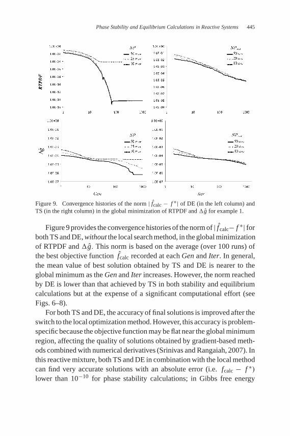
Figure 9. Convergence histories of the norm | fcalc − f ∗| of DE (in the left column) andTS (in the right column) in the global minimization of RTPDF and �g for example 1.

Figure 9 provides the convergence histories of the norm of | fcalc− f ∗| forboth TS and DE, without the local search method, in the global minimizationof RTPDF and �g. This norm is based on the average (over 100 runs) ofthe best objective function fcalc recorded at each Gen and Iter. In general,the mean value of best solution obtained by TS and DE is nearer to theglobal minimum as the Gen and Iter increases. However, the norm reachedby DE is lower than that achieved by TS in both stability and equilibriumcalculations but at the expense of a significant computational effort (seeFigs. 6–8).

For both TS and DE, the accuracy of final solutions is improved after theswitch to the local optimization method. However, this accuracy is problem-specific because the objective function may be flat near the global minimumregion, affecting the quality of solutions obtained by gradient-based meth-ods combined with numerical derivatives (Srinivas and Rangaiah, 2007). Inthis reactive mixture, both TS and DE in combination with the local methodcan find very accurate solutions with an absolute error (i.e. fcalc − f ∗)lower than 10−10 for phase stability calculations; in Gibbs free energy



minimization, this absolute error is around 10−10 for DE and is slightlylower than 10−7 for TS. The use of direct search methods (e.g. Nelder–Mead simplex method) for local optimization at the end of TS and DEis a suitable option for handling objective functions that are flat near theglobal minimum. However, these local search strategies are known to beless efficient than the gradient-based methods. With respect to algorithmefficiency, CPUt ranged from 0.01 to 2.09 seconds for DE, and from 0.01 to0.08 seconds for TS in all stability and equilibrium calculations performed.

Finally, we have solved the phase stability and equilibrium problemsin this example using the quasi-Newton method alone with random initialvalues (100 runs for each problem). This local solver generally convergedto trivial solutions, with only 42% SR for phase stability and 16% SRfor equilibrium calculations. When the method converged to the globalsolution, it required an average of 351 NFE for phase stability and 156NFE for equilibrium calculations (CPUt < 0.001 s). As expected, the quasi-Newton method is more efficient than DE and TS but less reliable for findingthe global minimum and dependent on the initial values. Therefore, thisand other local methods are not suitable for phase stability and equilibriumcalculations in reactive systems.

5.2. Example 2

This example refers to the esterification reaction of ethanol and acetic acidto form ethyl acetate and water:

ethanol (1) + acetic acid (2) ↔ ethyl acetate (3) + water (4). (32)

This system is a benchmark problem for testing algorithms in phase equilib-rium calculations for reactive systems (e.g. Castillo and Grossmann, 1981;Xiao et al., 1989; McDonald and Floudas, 1996; Lee et al., 1999; Jalaliet al., 2008). In this study, water is selected as the reference component forcomposition transformation, and transformed variables are given by:

X1 = x1 + x4, (33)

X2 = x2 + x4, (34)

X3 = x3 − x4, (35)

where X1, X2 ∈ (0, 1) and X3 ∈ (−1, 1). We use the NRTL model forcalculating the thermodynamic properties of the liquid phase, while the



vapor phase is assumed to be ideal where the dimerization of acetic acid isnot considered (see thermodynamic data in Table B5 of Appendix B).

Three feeds are analyzed at different temperatures and 1 atm. First,we consider an equi-molar feed of ethanol and acetic acid, ni,F =(0.5, 0.5, 0.0, 0.0) at 358 K. So, the transformed composition Zi =(0.5, 0.5, 0.0), where ni,F = (0.5, 0.5, 0.0) and nT,F = 1.0, is testedfor phase stability. In these conditions, the chemical equilibrium constantfor this reaction is Keq,1 = 18.154056, which was calculated using the ther-modynamic data reported by Lee et al. (1999), and this feed correspondsto a vapor phase (McDonald and Floudas, 1996; Lee et al., 1999). Thus,RTPDF is defined as:

RTPDF = X1

(�µ1

RT

∣∣∣∣X

− ln

(z1 P

Psat1

))+ X2

(�µ2

RT

∣∣∣∣X

− ln

(z2 P

Psat2

)),

+ X3

(�µ3

RT

∣∣∣∣X

− ln

(z3 P

Psat3

)), (36)

where the chemical potential at X is obtained from Eq. (25) with �g1 and�g2 given by

�g1 =3∑

i=1

Xi ln(xiγi ), (37)

�g2 =3∑

i=1

Xi ln

(xi P

Psati

), (38)

for liquid and vapor phases respectively. Note that z in Eq. 36 are the chem-ically equilibrated mole fractions, and are obtained from variable transfor-mation Z → z (see Appendix A).

Phase stability analysis is performed using Eq. (36) and two decisionvariables: X1, X2(0, 1); and X3 is calculated using X3 = 1 − X1 − X2. Inthese calculations, we use the following parameters for stochastic methods:(a) DE: A = 0.3, CR = 0.9, NP = 50nvar, Genmax = 50 and Scmax =6nvar; and (b) TS: Nt = N p = 5, εt = εp = 0.005, NPinit = 20nvar,Itermax = 50nvar, hn = 0.5 and Scmax = 12nvar , where nvar = 2. Resultsof stability calculations are reported in Table 4. Since the global minimumof RTPDF is 0.0 at the trivial solution Zi = Xi , this feed is stable. Thisresult is consistent with that reported by Xiao et al. (1989), McDonald and



Floudas (1997) and Lee et al. (1999). Both TS and DE in combination withthe local method, find the global solution of this stability problem with100% SR, and TS is more efficient than DE (see Table 4).

Now, the same feed, ni,F = (0.5, 0.5, 0.0, 0.0) is analyzed at 355 Kwith Keq,1 = 18.670951 where both the liquid and vapor exists (Xiaoet al., 1989; McDonald and Floudas, 1996; Lee et al., 1999). Again, Keq,1

is determined from thermodynamic data reported by Lee et al. (1999).Stability calculations are performed using Eqs. (36) to (38) and the samedecision variables; the results of stability analysis are reported in Table 4.Again, both TS and DE are reliable to determine that this mixture is unstable,and TS is more efficient than DE.

Considering the results of stability criterion, we have performed theminimization of transformed Gibbs free energy for calculating the phaseequilibrium:

�g = n1,1�µ1,1

RT+ n2,1

�µ2,1

RT+ n3,1

�µ3,1

RT+ n1,2

�µ1,2

RT

+ n2,2�µ2,2

RT+ n3,2

�µ3,2

RT, (39)

where the chemical potentials are defined by Eqs. (25), (37) and (38). Forthis feed, recall that ni,F = (0.5, 0.5, 0.0) and nT,F = 1.0, and as a con-sequence n3,2 = −n3,1. We can define the transformed moles of phase 1as a fraction of total transformed moles in the feed (i.e. nT,1 = nT,FλF

where λF ∈ (0, 1)). So, the global optimization of �g is performed withrespect to three decision variables: λ1,1, λ2,1 ∈ (0, 1) and λF ∈ (0, 1). Thetransformed mole numbers are given by:

n1,1 = 0.5λ1,1

n2,1 = 0.5λ2,1, (40)

n3,1 = nT,FλF − (n1,1 + n2,1)

and Eq. (9) is used to determine ni,2.In these calculations, the parameters of DE and TS are the same as those

for phase stability calculations except Genmax = 75, Itermax = 100nvar,and Scmax = 12nvar where nvar = 3. These parameter values have been



Tabl

e4.

Res

ults

ofph

ase

stab

ilit

yan

deq

uili

briu

mca

lcul

atio

nsfo

rex

ampl

e2

usin

gT

San

dD

E.

Fee

dS

R(%

)fo

rN

FE

(CP

Ut,

s)fo

r

ZT

,KG

loba

lopt

imum

DE

TS

DE

TS

(0.5

,0.5

,0)

358

RT

PD

F=

0.0

atX

i=

(0.5

,0.

5,0)

orx

=(0

.075

325,

0.07

5325

,0.

4246

75,

0.42

4675

)10

010

051

1253

6(1

.4)

(0.1

4)

355

RT

PD

F=

−0.0

3205

7at

Xi=

(0.7

2739

1,0.

8928

42,−0

.620

233)

orx

=(0

.035

139,

0.20

0590

,0.

0720

19,

0.69

2252

)10

099

5178

550

(1.3

)(0

.14)

�g

=−2

.058

125

atX

i,1

=(0

.716

726,

0.87

8827

,−0

.595

553)

and

Xi,

2=

(0.4

8879

8,0.

4804

20,

0.03

0782

);or

x i,1

=(0

.078

272,

0.06

9894

,0.

4413

08,

0.41

0526

)an

dx i

,2=

(0.0

3974

8,0.

2018

49,

0.08

1425

,0.

6769

78)

240

1062

3—

(5.9

)

(0.2

,0.4

,0.4

)35

5R

TP

DF

=−0

.223

934

atX

i=

(0.1

4645

2,0.

7320

01,

0.12

1547

)or

x=

(0.0

1035

4,0.

5959

04,

0.25

7644

,0.

1360

98)

100

100

5178

524

(1.3

)(0

.13)

�g

=−1

.302

752

atX

i,1

=(0

.163

826,

0.57

5748

,0.

2604

26)

and

Xi,

2=

(0.2

1755

7,0.

3147

00,

0.46

7743

);or

x i,1

=(0

.023

539,

0.43

5461

,0.

4007

13,

0.14

0287

)an

dx i

,2=

(0.0

2943

5,0.

1265

77,

0.65

5865

,0.

1881

23)

100

7411

592

780

(6.1

)(0

.41)



modified because phase equilibrium problems are generally more difficultto solve compared to stability ones (Srinivas and Rangaiah, 2007). Resultsfor these calculations are also reported in Table 4. In this case, both DEand TS face difficulties in finding the global minimum of �g; SR of DE is24% whereas TS fails to find the global minimum. This problem is chal-lenging due to the presence of a trivial solution (Zi = Xi,1 = Xi,2) whichhas an objective value (−2.057331) very comparable to the global mini-mum (−2.058125). Phase equilibrium compositions given in Table 4 areconsistent with those reported by McDonald and Floudas (1996) and Leeet al. (1999). Note that there are differences between the objective functionvalues in Table 4 and those given in these references because the previousworks incorporated the Gibbs free energies of formation into the objectivefunction (i.e. the total Gibbs free energy) while we have used the trans-formed Gibbs free energy of mixing as the objective. Both approaches areequivalent and can be used for phase equilibrium calculations in reactivesystems.

Finally, consider a vapor mixture of ethanol, acid acetic, and ethylacetate with initial composition of ni,F = (0.2, 0.4, 0.4, 0.0) at 355 K and1 atm. At these conditions, Zi = (0.2, 0.4, 0.4), ni,F = (0.2, 0.4, 0.4) andnT,F = 1, and this mixture also shows a vapor-liquid equilibrium withKeq,1 = 18.670951. Stability test is performed using Eqs. (36)–(38) andthe same decision variables as in the previous feeds. Both TS and DE arecapable of finding the global optimum of RTPDF without any difficulty(Table 4). Based on stability result, we have performed the minimizationof transformed Gibbs free energy using Eqs. (25), (37)–(39). The globaloptimization of �g is performed with respect to three decision variablesλi,1 ∈ (0, 1). The transformed mole numbers are given by:

n1,1 = 0.2λ1,1

n2,1 = 0.4λ2,1, (41)

n3,1 = 0.4λ3,1

and Eq. (9) is used to determine ni,2. The results of Gibbs energy mini-mization are summarized in Table 4. DE is 100% reliable, but it requiressignificant computational effort; although TS is very efficient, it may failto find the equilibrium compositions as shown in Table 4.



5.3. Discussion

In this study, relative performance of TS and DE is in accordance with thatreported for equilibrium calculations of non-reactive mixtures (Srinivas andRangaiah, 2007). The differences between the performance of TS and DEmay be associated with the efficacy of their escaping strategies. DE appliesmutation and crossover strategies on a specific population to diversify thesearch and to escape from the local optimum. In this algorithm, the bestsolution that has been identified over all generations is reported after sat-isfying the convergence criterion. On the contrary, TS uses the best pointin each iteration to create the new test points and to escape from the localsolution, even though the current best solution may be worse than the bestsolutions found in the earlier iterations.

For comparison purposes, we have solved examples 1 and 2 using theSA method (Bonilla-Petriciolet et al., 2006) with the following coolingschedule: initial annealing temperature = 10, number of iterations beforereduction of annealing temperature = 5, and temperature reduction factor =0.85. Each example was solved using 100 trials with random initial valuesvia random number seed. Results of these calculations are summarized inTable 5. It appears that DE and TS are better than SA in terms of both NFEand CPUt but the order of reliability of these methods is: SA > DE > TSin both reactive phase stability and equilibrium calculations.

Table 5. Performance comparison of SA, DE and TS for reactive phase stability andequilibrium calculations for examples 1 and 2.

SA DEa TSa

Objective function SR,% NFE CPUt SR,% NFE CPUt SR,% NFE CPUt

Example 1 RTPDF 100 23869 0.33 100 7677 0.07 86 595 0.004�g 92 22201 0.53 74 10841 0.15 26 578 0.008

Example 2 RTPDFb 100 18163 6.1 100 5112 1.4 100 536 0.14RTPDFc 100 17305 5.6 100 5178 1.3 99 550 0.14�gc 44 26319 17.5 24 10623 5.9 0 — —RTPDFd 100 17005 5.7 100 5178 1.3 100 524 0.13�gd 100 27106 17.7 100 11592 6.1 74 780 0.41

a Parameters of TS and DE are those described in Example 2;b Results for feed Zi = (0.5, 0.5, 0.0) at 358 K and 1 atm;c Results for feed Zi = (0.5, 0.5, 0.0) at 355 K and 1 atm;d Results for feed Zi = (0.2, 0.4, 0.4) at 355 K and 1 atm.



6. Conclusions

This study shows, for the first time, that both TS and DE can be successful,if they are properly implemented, for solving phase stability and equi-librium calculations in multi-component and multi-reactive systems usingtransformed composition variables. Also, we demonstrate that performanceprofiles can be used to systematically tune the algorithm parameters of thesemethods. In general, the performance of DE is better than TS, but requiresmore NFE and CPUt. For both stability and equilibrium calculations, themaximum number of generations/iterations significantly affects the perfor-mance of these stochastic methods. Depending on problem characteristics,proper value for the termination criterion: Scmax and the maximum numberof generations/iterations should be selected to improve the performance ofthese stochastic methods.

References

Ali, M.M., Khompatraporn, C. and Zabinsky, Z.B. (2005). A numerical evaluationof several stochastic algorithms on selected continuous global optimization testproblems. Journal of Global Optimization, 31, pp. 635–672.

Baker, L.E., Pierce, A.C. and Luks, K.D. (1982). Gibbs energy analysis of phaseequilibria. Society of Petroleum Engineers Journal, 22, pp. 731–742.

Bonilla-Petriciolet, A., Bravo-Sanchez, U.I., Castillo-Borja, F., Frausto-Hernandez, S. and Segovia-Hernandez, J.G. (2008). Gibbs energy minimizationusing simulated annealing for two-phase equilibrium calculations in reactivesystems. Chemical and Biochemical Engineering Quarterly, 22, pp. 285–298.

Bonilla-Petriciolet, A., Vazquez-Roman, R., Iglesias-Silva, G.A. and Hall, K.R.(2006). Performance of stochastic optimization methods in the calculation ofphase stability analyses for nonreactive and reactive mixtures. Industrial andEngineering Chemistry Research, 45, pp. 4764–4772.

Burgos-Solorzano, G.I., Brennecke, J.F. and Stadtherr, M.A. (2004). Validatedcomputing approach for high-pressure chemical and multiphase equilibrium.Fluid Phase Equilibria, 219, pp. 245–255.

Castier, M., Rasmussen, P. and Fredenslund, A. (1989). Calculation of simultane-ous chemical and phase equilibria in nonideal systems. Chemical EngineeringScience, 44, pp. 237–248.

Castillo, J. and Grossmann, I.E. (1981). Computation of phase and chemical equi-libria. Computers and Chemical Engineering, 5, pp. 99–108.

Dennis, J.E. Jr. and Schnabel, R.B. (1983). Numerical Methods for UnconstrainedOptimization and Nonlinear Equations. Prentice-Hall, Englewood Cliffs, NewJersey.



Dolan, E.D. and More, J.J. (2002). Benchmarking optimization softwarewith performance profiles. Mathematical Programming Series A, 91,pp. 201–213.

Gupta, A.K., Bishnoi, P.R. and Kalogerakis, N. (1991). A method for the simul-taneous phase equilibria and stability calculations for multiphase reacting andnon-reacting systems. Fluid Phase Equilibria, 63, pp. 65–89.

Iglesias-Silva, G.A., Bonilla-Petriciolet, A. and Hall, K.R. (2006). An algebraicformulation for an equal area rule to determine phase compositions in simplereactive systems. Fluid Phase Equilibria, 241, pp. 25–30.

Jalali, F. and Seader, J.D. (1999). Homotopy continuation method in multi-phasemulti-reaction equilibrium systems. Computers and Chemical Engineering, 23,pp. 1319–1331.

Jalali-Farahani, J. and Seader, J.D. (2000). Use of homotopy-continuation methodin stability analysis of multiphase, reacting systems. Computers and ChemicalEngineering, 24, pp. 1997–2008.

Jalali, F., Seader, J.D. and Khaleghi, S. (2008). Global solution approaches inequilibrium and stability analysis using homotopy continuation in the complexdomain. Computers and Chemical Engineering, 32, pp. 2333–2345.

Lee, Y.P., Rangaiah, G.P. and Luus, R. (1999). Phase and chemical equilibrium cal-culations by direct search optimization. Computers and Chemical Engineering,23, pp. 1183–1191.

McDonald, C.M. and Floudas, C.A. (1996). GLOPEQ: A new computational toolfor the phase and chemical equilibrium problem. Computers and ChemicalEngineering, 21, pp. 1–23.

McKinnon, K. and Mongeau, M. (1998). A generic global optimization algorithmfor the chemical and phase equilibrium problem. Journal of Global Optimiza-tion, 12, pp. 325–351.

Michelsen, M.L. (1982). The isothermal flash problem. Part I. Stability. FluidPhase Equilibria, 9, pp. 1–19.

Perez-Cisneros, E.S., Gani, R. and Michelsen, M.L. (1997). Reactive separationsystems-I. Computation of physical and chemical equilibrium. Chemical Engi-neering Science, 52, pp. 527–543.

Rangaiah, G.P. (2001). Evaluation of genetic algorithms and simulated annealingfor phase equilibrium and stability problems. Fluid Phase Equilibria, 187–188,pp. 83–109.

Reynolds, D., Mulholland, A.J. and Gomatam, J. (1997). Calculation of chem-ical and phase equilibria via simulated annealing. Journal of MathematicalChemistry, 22, pp. 25–37.

Seider, W.D. and Widagdo, S. (1996). Multiphase equilibria of reactive systems.Fluid Phase Equilibria, 123, pp. 283-303.

Srinivas, M. and Rangaiah, G.P. (2007). A study of differential evolution and tabusearch for benchmark, phase equilibrium and phase stability problems. Com-puters and Chemical Engineering, 31, pp. 760–772.



Stateva, R.P. and Wakeham, W.A. (1997). Phase equilibrium calculations for chem-ically reacting systems. Industrial and Engineering Chemistry Research, 36,pp. 5474–5482.

Taylor, R. and Krishna, R. (2000). Modelling reactive distillation. Chemical Engi-neering Science, 55, pp. 5183–5229.

Teh, Y.S. and Rangaiah, G.P. (2003). Tabu search for global optimization of contin-uous functions with application to phase equilibrium calculations. Computersand Chemical Engineering, 27, pp. 1665–1679.

Ung, S. and Doherty, M.F. (1995a). Vapor-liquid phase equilibrium in systems withmultiple chemical reactions. Chemical Engineering Science, 50, pp. 23–48.

Ung, S. and Doherty, M.F. (1995b). Theory of phase equilibria in multireactionsystems. Chemical Engineering Science, 50, pp. 3201–3216.

Xiao, W., Zhu, K., Yuan, W. and Chien, H.H. (1989). An algorithm for simul-taneous chemical and phase equilibrium calculations. AlChE Journal, 35,pp. 1813–1820.

Xu, G., Haynes, W.D. and Stadtherr, M.A. (2005). Reliable phase stability analysisfor asymmetric models. Fluid Phase Equilibria, 235, pp. 152–165.

Wakeham, W.A. and Stateva, R.P. (2004). Numerical solution of the isothermal,isobaric phase equilibrium problem. Reviews in Chemical Engineering, 20,pp. 1–56.

Wasylkiewicz, S.K. and Ung, S. (2000). Global phase stability analysis for hetero-geneous reactive mixtures and calculation of reactive liquid-liquid and vapor-liquid-liquid equilibria. Fluid Phase Equilibria, 175, pp. 253–272.

7. Exercises

(1) Consider a hypothetical reacting ternary mixture A1 + A2 ⇔ A3

with liquid-liquid equilibrium (Iglesias-Silva et al., 2006), where reac-tion equilibrium constant is independent of temperature, and ther-modynamic properties are calculated using the Margules solutionmodel Gex

RT = 3.6x1x2 + 2.4x1x3 + 2.3x2x3. This system showscomplex equilibrium behavior for some values of the reaction equi-librium constant. The third component is selected as the referencesubstance. For a transformed feed Zi = (0.6, 0.4), nT,F = 1.0and Keq,1 = 0.9825, determine if this mixture is stable; if it isnot stable, calculate the corresponding equilibrium compositions.Use both TS and DE, and compare their performance for differ-ent values of NP, NPinit, Itermax and Genmax. [Solution: RTPDF= −0.020055 at Xi = (0.83575, 0.16425); �g = −0.144508 atXi,1 = (0.484538, 0.515462) and Xi,2 = (0.815044, 0.184956)].



(2) Consider a six-component mixture with only one chemical reaction2A5 ⇔ A6 but with four inert components: A1, A2, A3 and A4. Thismixture shows vapor-liquid equilibrium at 75◦C and 1.5 atm where thereaction equilibrium constant is 5.0. Assume that the vapor and liq-uid phases behave as an ideal gas and ideal solution, thermodynamicdata are given in Table B4, and choose component A6 as the referencefor calculating the transformed mole fractions. Establish the equilib-rium compositions for a transformed feed Zi = (0.00497, 0.605, 0.0324,0.31, 0.04763) and nT,F = 1.0 using both TS and DE. Construct thequartile sequential plots for different values of NP and NPinit . Performat least 25 runs with random initial values for this purpose. Compare anddiscuss the results obtained from these trials. Which of the two methodsis better, and why? [Solution: RTPDF=−0.004072 at Xi = (0.005931,0.736912, 0.033105, 0.180695, 0.043356); �g = −0.144508 atXi,1 = (0.004923, 0.598568, 0.032360, 0.316323, 0.047827) andXi,2 = (0.005899, 0.732032, 0.033198, 0.185129, 0.043742)].

Appendix A

To illustrate the application of the transformation procedure of Ung andDoherty (1995a, 1995b), consider a ternary mixture that follows the reac-tion: A1 + A2 ↔ A3. For this system, we have c = 3, r = 1 and c − r = 2transformed composition variables. For variable transformation, it is nec-essary to select a set of r reference components such that N is an invertiblematrix. This requires that all the reactions must involve at least one of thereference components, an inert component can not be a reference compo-nent and no two reference components can have identical stoichiometriccoefficients in each reaction (Ung and Doherty, 1995a).

If A3 is selected as the reference component, N is invertible and equalto unity. In this case, v1 = −1, v2 = −1, and vTOT = −1, and so thetransformed mole numbers and fractions are given by:

n1 = n1 + n3, (A1)

n2 = n2 + n3, (A2)



X1 = n1

nT= n1 + n3

nT + n3= x1 + x3

1 + x3, (A3)

X2 = n2

nT= n2 + n3

nT + n3= x2 + x3

1 + x3= 1 − X1, (A4)

where nT = n1 + n2 + n3, nT = n1 + n2 and X1, X2 ∈ [0, 1]. Note that,for this mixture, any of the three components can be used as the referencecomponent to define the transformed composition variables (n and X).

If the initial composition (mole numbers or fractions) of the reac-tive mixture is available, the corresponding transformed variables can beobtained by using the above equations. For example, consider a mixture withinitial composition: ni,F = (0.3, 0.2, 0.5). Using Eqs. (A1)–(A4), trans-formed mole numbers are: n1,F = 0.3 + 0.5 = 0.8, n2,F = 0.2 + 0.5= 0.7, and nT,F = 0.8 + 0.7 = 1.5; while transformed mole fractions are:Z1 = 0.8/1.5 ∼= 0.5333 and Z2 = 0.7/1.5 = 1 − Z1

∼= 0.4667.

The transformed composition variables take the same value before, dur-ing and after reaction (Ung and Doherty, 1995a) but depend on the initialcomposition. Therefore, the mole fractions that are chemically equilibrated,satisfy the stoichiometry requirements and corresponding to Z must beobtained. To do this, we need to find the composition of reference compo-nents that satisfy the chemical equilibrium constraints. In the general case,for a set of c − r specified transformed variables Xi , the reference molefractions xref are calculated using Eq. (5) and the equilibrium constants foreach reaction Keq,k ; this requires solution of r nonlinear equations givenby Eq. (6) because Keq,k are non-linear functions of x . After knowing xref ,the corresponding mole fractions of c − r non-reference components arecalculated using Eq. (5) again. For this transformation procedure X → x ,any solver such as the bisection method (for systems with only one reaction)or the Newton method (for multi-reaction systems) can be used to find xref .Figure A1 presents the steps in the variable transformation between X andx . Note that if different models are used in the calculation of thermodynamicproperties for the different phases, the procedure of variable transformationmust be performed for each model at specified X . In these cases, the molefraction x that corresponds to the lower value of transformed Gibbs freeenergy is selected.

For illustrative purposes, let us consider that this ternary mixture is anideal liquid phase (i.e. γi = 1.0). The chemical equilibrium constant is



1. Start with the specified components, composition (mole numbers or fractions) of reactive mixture, T, P and the thermodynamic models.

2. Select r reference components, and determine N and N-1. Calculate the equilibrium constant,

keqK ,of each of all reactions at the given T using relevant thermodynamic

equations (e.g. see Table 2).

3. Calculate X using Eqs. (3) −

− −

(5), and choose initial values for refx .

4. Using refx , c r values of Xi obtained in step 3, and rearranged Eq. (5): xi = Xi (1

vTOT N-1xref ) + vi N-1xref, determine mole fractions of non-reference components.

5. Calculate the activity, ai of each of all components using the specified thermodynamic model for the phase and xi found in Step 4.

6. Substitute values of equilibrium constants and activities in the r non-linear equations (Eq. 6). If these equations are not satisfied, use any solver such as the bisection method(for situations with only one reaction) or the Newton method (for multi-reactionsystems) to find new values of ,refx and then go to step 4. Note that the gradient for the

Newton method can be calculated via finite differences.

7. If the r non-linear equations are satisfied to the desired tolerance level, current valuesof x are chemically equilibrated and satisfy the stoichiometry and equilibriumrequirements.

Figure A1. Steps in the composition transformation procedure X → x .

defined as

Keq,1 = a3

a1a2= x3γ3

x1γ1x2γ2. (A5)

We can rearrange Eqs. (A3) and (A4) to obtain

xi = Xi (1 + x3) − x3 for i = 1, 2. (A6)

Substituting Eq. (A6) into Eq. (A5), we find

f (x3) = Keq[X1(1 + x3) − x3][X2(1 + x3) − x3]γ1γ2 − x3γ3 = 0.

(A7)

Therefore, if we specify X , mole fractions x that simultaneously satisfythe chemical equilibrium equation and map onto the specified values of thetransformed composition variables are determined by solving Eq. (A7) forthe reference component x3. For our example, if Keq,1 = 1.0, γi = 1.0and Zi = (0.5333, 0.4667), solving f (x3) we find chemically equilibratedmole fractions in the given feed as zi = (0.4537, 0.3758, 0.1705). Notethat these are not the given mole fractions in the feed but are chemicallyequilibrated mole fractions.



Now, consider this mixture but with the presence of liquid-liquid equi-librium while the reaction occurs at 323.15 K and Keq,1 = 3.5. In theseconditions, we calculate the activity coefficient γi using the Margules solu-tion equation:

T ln γk = 1

2

c∑i=1

c∑j=1

(Aik + Ajk − Aij)xi x j , (A8)

with Aij = Aji, Aii = 0.0, A12 = 478.6, A13 = 1074.484 andA23 = 626.9. Note that Margules model is used to represent the liquid-phase non-idealities because there is no phase split (i.e. liquid-liquid phaseequilibrium) for an ideal liquid (i.e. γi = 1.0). The chemical potentialof each component and the transformed Gibbs free energy of mixing arerespectively

�µi

RT= ln(xiγi), (A9)

�g1 = X1 ln(x1γ1) + X2 ln(x2γ2), (A10)

where xi results from X → x using Eqs. (A5)–(A7). Note that f (x3) is anon-linear function with x3 as unknown and has to be solved for given X .

Figure A2 shows the plot of �g1 versus X1 for this mixture. This plotis obtained by varying X1 from 0.0 to 1.0, calculating the associated molefractions x for each X1 (using Algorithm of Fig. A1), and evaluating �g1

(Eq. A10). As shown in this figure, this reactive mixture exhibits a phasesplit for Z1 between 0.497527 and 0.840050. Any trial composition insidethis range will show phase equilibrium. For our analysis, we have selectedthe same feed Zi = (0.5333, 0.4667) and nT,F = 1.0. To evaluate phasestability, we need to minimize the reactive plane distance function, obtainedfrom Eqs. (10) and (A9):

RTPDF = X1(ln(x1γ1) − ln(z1γ1))+X2(ln(x2γ2) − ln(z2γ2)). (A11)

Note that RTPDF can be optimized with respect to X1 ∈ (0, 1) because X2

is obtained from the equality constraint: X2 = 1− X1. The global optimumfor this feed is −0.406606 at Xi = (0.9527, 0.0473). As expected, the givenfeed is unstable.



g∆

-0.8

-0.6

-0.4

-0.2

0.0

0.0 0.2 0.4 0.6 0.8 1.0

Equilibrium compositions

Feed

X1

Figure A2. Transformed molar Gibbs free energy of mixing versus X1 for reactive mixture:A1 + A2 ↔ A3 at 323.15 K and Keq,1 = 3.5.

For performing phase equilibrium calculations, the Gibbs free energyfunction is obtained from Eqs. (1) and (A9) as:

�g = n1,1 ln(x1,1γ1,1) + n2,1 ln(x2,1γ2,1)

+ n1,2 ln(x1,2γ1,2) + n2,2 ln(x2,2γ2,2), (A12)

where ni, j is the transformed mole number of component i in liquid phasej . Note that the transformation procedure X → x is performed for eachliquid phase, taking into account its corresponding transformed composi-tion ni, j . We have two decision variables: λ1,1 and λ2,1 for this example.They are used to calculate n1,1 = 0.5333λ1,1 and n2,1 = 0.4667λ2,1

as well as the transformed composition of the second liquid phase byn1,2 = 0.5333−0.5333λ1,1 and n2,2 = 0.4667−0.4667λ1,1 (Eqs. 7 and 9).The global optimum of �g is −0.639429 at Xi,1 = (0.497527, 0.502473)

and Xi,2 = (0.840050, 0.15995), which are the transformed mole frac-tions at liquid-liquid equilibrium; the equilibrium compositions in con-ventional mole fractions are: xi,1 = (0.056907, 0.066186, 0.876907) andxi,2 = (0.829728, 0.105473, 0.064529).

Appendix B

Thermodynamic data and model parameters for all reactive systems usedin this chapter are given in Tables B1–B5.



Tabl

eB

1.T

herm

odyn

amic

data

for

the

met

hylt

ert-

buty

leth

er(M

TB

E)

reac

tion

syst

emw

ith

iner

tat1

0at

man

d37

3.15

K.

Para

met

ers

ofpu

reco

mpo

nent

u ij

inth

eW

ilso

nm

odel

(cal

/mol

)

Com

pone

nt1

Ai

Bi

Ci

Vi

12

34

16.

8413

292

3.20

123

9.99

93.3

3—

169.

9953

−60.

1022

—2

8.07

372

1578

.23

239.

382

44.4

425

76.8

532

—14

83.2

478

2283

.872

63

6.87

201

1116

.825

224.

744

118.

827

1.56

69−4

06.3

902

——

46.

8089

693

5.86

238.

7310

0.39

—38

2.34

29—

—

log 1

0P

sat

i=

Ai−

Bi

T+C

iw

here

Psa

ti

inm

mH

gan

dT

in◦ C

.

lnγ

i=

1−l

n( ∑

c j=1

xj�

ij

) −∑ c k=1

( x k�

ki/∑ c j=

1x

j�kj

)

�ij

=V

jV

iex

p( −u

ijR

T

)K

eq,1

=a 3 a 1a 2

whe

rea i

=x i

γi

for

liqu

idph

ase

and

a i=

x iP

/P

sat

ifo

rva

por

phas

e.

11:

Isob

uten

e,2:

Met

hano

l,3:

MT

BE

,and

4:B

utan

e.



Tabl

eB

2.T

herm

odyn

amic

data

for

the

reac

tive

syst

emfo

rte

rt-a

myl

met

hyle

ther

(TA

ME

)sy

nthe

sis

at33

5K

and

1.5

atm

.

Para

met

ers

ofpu

reco

mpo

nent

u ij

inth

eW

ilso

nm

odel

(cal

/mol

)

Com

pone

nt1

Ai

Bi

Ci

Di

Vi

12

34

174

.527

−523

2.2

−8.1

482

8.47

4E-0

60.

1086

8—

478.

813

76.5

−611

.75

282

.614

−558

6.1

−9.4

429

1.08

58E

-05

0.10

671

−477

.94

—96

8.81

−386

.04

323

.534

7−3

661.

468

−32.

770.

0406

997

72.3

1014

7—

4826

.34

20.9

441

−293

6.22

3−4

7.70

385

0.13

345

951.

3371

2.33

−177

—

lnP

sat

i=

Ai+

Bi T+

Ci

lnT

+D

iT2

for

i=

1,2

lnP

sat

i=

Ai+

Bi

T+C

ifo

ri=

3,4

whe

reP

sat

iin

Paan

dT

inK

elvi

n.

lnγ

i=

1−

ln( ∑

c j=1

xj�

ij

) −∑ c k=

1

( x k�

ki

/ ∑c j=

1x

j�kj

)

�ij

=V

jV

iex

p( −u

ijR

T

)

Keq

,1=

a2 4

a 1a 2

a2 3

whe

rea i

=x i

γi

for

liqu

idph

ase

and

a i=

x iP

/P

sat

ifo

rva

por

phas

e.

11:

2-M

ethy

l-1-

bute

ne,2

:2-M

ethy

l-2-

bute

ne,3

:Met

hano

l,an

d4:

TAM

E.



Table B3. Thermodynamic data for the reaction for butyl acetate production at 298.15 Kand 1 atm.

uij in the UNIQUAC model (cal/mol)

Component1 Q Ru 1 2 3 4

1 2.072 2.2024 — −131.7686 −343.593 −298.43442 3.052 3.4543 148.2833 — 68.0083 82.53363 1.4 0.92 527.9269 581.1471 — 394.23964 4.196 4.8724 712.2349 24.6386 756.4163 —

ln γi = ln γ Ei + ln γ R

i

ln γ Ei = ln φi

xi+ 5Qi ln φi

xi+ li − φi

xi

∑cj=1 x j l j

ln γ Ri = Qi

(1 − ln

(∑cj=1 θ j τji

)− ∑c

j=1

(θ jτji∑c

l=1 θlτli

))

θi = Qi xi∑cj=1 Q j x j

φi = Ru,i xi∑cj=1 Ru, j x j

li = 5(Ru,i − Qi )− (Ru,i −1) Keq,1 = a3a4a1a2

where ai = xi γi .

1 1: Acetic acid, 2: n-Butanol, 3: Water, and 4: n-Butyl acetate.

Table B4. Thermodynamic data for Example 1.

Component Ai Bi Ci γi

1 7.6313 1566.69 273.419 1.02 7.11714 1210.595 229.664 1.03 7.44777 1488.99 264.915 1.04 8.1122 1592.864 226.184 1.05 7.9701 1521.23 233.97 1.06 6.8664 1188.05 226.276 1.0

log10 Psati = Ai − Bi

T +Ci

where Psati in mmHg and T in ◦C.

Keq,1 = a4a3

Keq,2 = a4a5

Keq,3 = a6a4

where ai = xi γi for liquid phase and ai = xi P/Psati for vapor phase.



Table B5. Thermodynamic data for Example 2.

Parameters of pure component τij in the NRTL model

Component1 Ai Bi Ci 1 2 3 4

1 9.95614 1440.52 −60.44 0.0 1.3941 0.6731 −0.20192 9.6845 1644.05 −39.63 −1.0182 0.0 0.007 −0.47353 9.22298 1238.71 −56.15 0.1652 0.5817 0.0 1.70024 10.09171 1668.21 −45.14 2.1715 1.6363 1.9257 0.0

log10 Psati = Ai − Bi

T +Ci

where Psati in N/m2 and

T in K.

αij = 0.3

ln γi =∑c

j=1 τjiGjix j∑cj=1 Gjix j

+∑c

j=1Gij x j∑c

l=1 Glj xl

(τij −

∑cl=1 τl j Gl j xl∑c

l=1 Glj xl

)

Gij = exp(−αijτij)Keq,1 = a3a4

a1a2where ai = xi γi for liquid phase and ai = xi P/Psat

ifor vapor phase.

1 1: Ethanol, 2: Acetic acid, 3: Ethyl acetate, and 4: Water.


Documents

Adrián Bonilla-Petriciolet Gade Pandu Rangaiah … libro...Juan Gabriel Segovia-Hernández and José Enrique Jaime-Leal Department of Chemical Engineering Universidad de Guanajuato,