Advanced Macroeconomics I ECON 525a - Fall 2009 …ordonez/pdfs/ECON 525a/ECON525a-4.pdfKiyotaki and Moore, JPE 97 Advanced Macroeconomics I ECON 525a - Fall 2009 Yale University Guillermo

Kiyotaki and Moore, JPE 97

Advanced Macroeconomics I

ECON 525a - Fall 2009

Yale University

Guillermo L. Ordonez

Week 4

Guillermo L. Ordonez Advanced Macroeconomics I ECON 525a - Fall 2009 Yale University


Introduction

Credit frictions → amplification & persistence of shocks

Two roles for capital

- Factor of production

- Collateral for loans

Negative productivity shock

- Reduces output; reduces value of collateral

- Reduces borrowing, which reduces output further

- ”Multiplier” effects amplifies losses



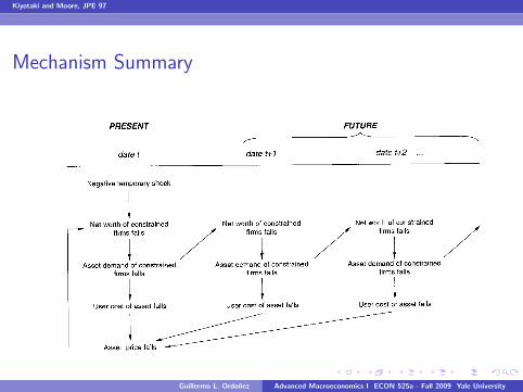
Mechanism Summary

credit cycles 213

Fig. 1

behavior of the constrained firms. They suffer a capital loss on theirlandholdings, which, because of the high leverage, causes their networth to drop considerably. As a result, the firms have to make yetdeeper cuts in their investment in land. There is an intertemporalmultiplier process: the shock to the constrained firms’ net worth inperiod t causes them to cut their demand for land in period t andin subsequent periods; for market equilibrium to be restored, theunconstrained firms’ user cost of land is thus anticipated to fall ineach of these periods, which leads to a fall in the land price in periodt ; and this reduces the constrained firms’ net worth in period t stillfurther. Persistence and amplification reinforce each other. Theprocess is summarized in figure 1.

In fact, two kinds of multiplier process are exhibited in figure 1,and it is useful to distinguish between them. One is a within-period,or static, multiplier. Consider the left-hand column of figure 1,marked ‘‘date t ’’ (ignore any arrows to and from the future). Theproductivity shock reduces the net worth of the constrained firms,and forces them to cut back their demand for land; the user costfalls to clear the market; and the land price drops by the sameamount (keeping the future constant), which lowers the value of thefirms’ existing landholdings, and reduces their net worth still fur-ther. But this simple intuition misses the much more powerful inter-temporal, or dynamic, multiplier. The future is not constant. As thearrows to the right of the date t column in figure 1 indicate, theoverall drop in the land price is the cumulative fall in present andfuture user costs, stemming from the persistent reductions in the



Agents

Farmers. measure 1

Et

∞∑s=0

βsxt+s

Gathers, measure m

Et

∞∑s=0

β′sx ′t+s

Farmers more impatient (β < β′)

(will imply that Farmers are the borrowers in equilibrium)

Both use land kt to produce fruit

Value of land ktqt used as collateral



Farmers

Farmers’ production function for fruit

yt+1 = (a + c)kt

akt = sellable fruit

ckt = ”bruised fruit” which must be consumed

Assume c > a( 1β − 1)

(in equilibrium farmer wants to consume ckt and sell akt)



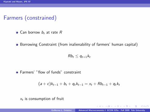
Farmers (constrained)

Can borrow bt at rate R

Borrowing Constraint (from inalienability of farmers’ human capital)

Rbt ≤ qt+1kt

Farmers’ ”flow of funds” constraint

(a + c)kt−1 + bt + qtkt−1 = xt + Rbt−1 + qtkt

xt is consumption of fruit



Gatherers (unconstrained)

They do not have specific skills to threat not paying.

Gatherers’ production function for fruit

y ′t+1 = G (k ′t)

G (·) has decreasing returns to scale

Gatherers’ budget constraint

G (k ′t−1) + b′t + qtk′t−1 = x ′t + Rb′t−1 + qtk

′t

x ′t is consumption of fruit



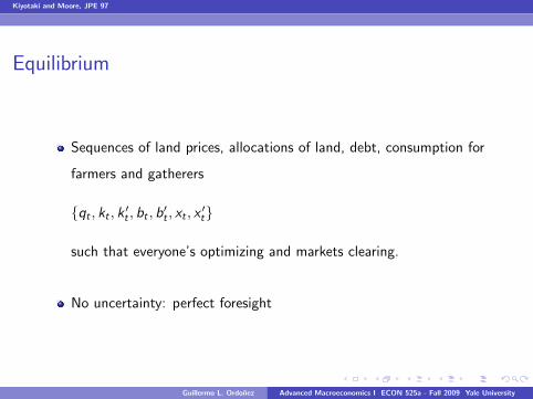
Equilibrium

Sequences of land prices, allocations of land, debt, consumption for

farmers and gatherers

{qt , kt , k′t , bt , b

′t , xt , x

′t}

such that everyone’s optimizing and markets clearing.

No uncertainty: perfect foresight



Equilibrium Results: Farmers

Farmers always borrow the maximum and invest in land

bt = qt+1kt/R and xt = ckt−1

Implied optimal land holdings

kt =1

qt − qt+1/R[(a + qt)kt−1 − Rbt−1]︸︷︷︸

net worth

ut ≡ qt − qt+1/R = ”down payment”

Farmers spend entire net worth on difference between price of new

land qt and amount against which they can borrow against each unit

of land qt+1/R



Equilibrium Results: Gatherers

Gatherer’s demand for land

G ′(k ′t)/R = ut = qt − (qt+1/R)︸︷︷︸user cost



Farmers in the Aggregate

Farmer aggregate landholding & borrowing

Kt =1

ut[(a + qt)Kt−1 − RBt−1]

Bt =1

Rqt+1Kt



Market Clearing

Land market resource constraint

mk ′t + Kt = K

Land market clearing

ut = qt − qt+1/R = G ′

1

m(K − Kt)︸︷︷︸

k′

/R

No bubbles in land price: lims→∞Et(R−sqt+s) = 0



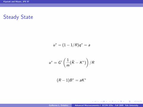
Steady State

u∗ = (1− 1/R)q∗ = a

u∗ = G ′(

1

m(K − K∗)

)/R

(R − 1)B∗ = aK∗



Steady Statecredit cycles 223

Fig. 2

ductivity of tradable output, a . As a result, farms neither expand norshrink.11

We are now in a position to compare consumption paths (8a),(8b), and (8c). In the steady state, the user cost equals a; and so,given the farmer’s discount factor β, investment gives him dis-counted utility βc/(1 2 β)a, saving gives Rβ2 c/(1 2 β)a, and con-sumption gives one. By assumption 1, investment strictly dominatessaving; and by assumption 2, investment strictly dominates consump-tion. This completes the proof of our earlier claim about farmers’optimal behavior in the neighborhood of the steady state.

Figure 2 provides a useful summary of the economy. On the hori-

11 Appealing to assumption 1, one can show that there is no steady-state equilib-rium in which the farmers’ credit constraints are not binding. (We are grateful toFrank Heinemann for pointing out to us that such an equilibrium can exist if β 5β′.) The model in the Appendix has no such equilibrium either, even though thefarmers and the gatherers have identical preferences.



One-time Productivity Shock with Credit Constraints

Say yt+1 = (1 + ∆)(a + c)kt

Period of shock (period t)

u(Kt)Kt = (a + ∆a + qt − q∗)K∗

Subsequent periods (periods t + s, s = 1, 2, ...)

u(Kt)Kt = (a + ∆a + qt − q∗)K∗



One-time Productivity Shock with Credit Constraints

Log-linearize around steady state

Define for variable Xt the proportional change from steady state

Xt =Xt − X ∗

X ∗

Period of shock (period t)

(1 + 1/η)Kt = ∆ +R

R − 1qt

Subsequent periods (periods t + s, s = 1, 2, ...)

(1 + 1/η)Kt+s = Kt+s−1

where η denotes elasticity of land supply of gatherers to user cost



Response of Land Price & Land Holdings

Land price response

qt =1

η∆

Overall land holding response

Kt =1

1 + 1η

(1 +R

R − 1

1

η)︸︷︷︸

>1

∆

Say η = 1, R = 1.05

Kt ≈ 11∆



Response of Land Price & Land Holdings

Land price response

qt =1

η∆


Kt =1

1 + 1η

(1 +R

R − 1

1

η)︸︷︷︸

>1

∆

Say η = 1, R = 1.05

Kt ≈ 11∆



Static Response of Land Price & Land Holdings

Land price response

qt |qt+1=q∗ =1

η

R − 1

R︸︷︷︸<1

∆


Kt |qt+1=q∗ = ∆



Response of Output & Productivity

Yt+s =a + c − Ra

a + c︸︷︷︸Productivity diff.

(a + c)K∗

Y ∗︸︷︷︸Farmers’ share

Kt+s−1



Net Worth Shock

One time reduction in debt obligations

Increases net worth

Farmer increases leverage, production

Another view of Bernanke-Paulson policies?



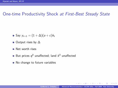
One-time Productivity Shock at First-Best Steady State

Say yt+1 = (1 + ∆)(a + c)kt

Output rises by ∆

Net worth rises

But prices q0 unaffected; land k0 unaffected

No change to future variables



Conclusions

Firms’ productive capital also used as collateral

Amplification of real shocks through lower collateral value of capital

Real effects of lower asset values



Critiques/Comments

Kocherlakota (QR, 2000): Quantitative importance likely to be

small if land & capital share less than 0.4

Andres Arias (WP, 2005): Calibrated RBC model with KM credit

constraints deliver small amplification effects

Does this work through ”investment wedge?” or TFP, or both?

Real effects of housing/stock bubbles


Documents

Advanced Macroeconomics I ECON 525a - Fall 2009 …ordonez/pdfs/ECON 525a/ECON525a-4.pdfKiyotaki and Moore, JPE 97 Advanced Macroeconomics I ECON 525a - Fall 2009 Yale University Guillermo