Advanced Opamp Topologies - CppSim · M.H. Perrott Summary of Single-Ended Versus Fully Differential Advantages of fully differential topologies-Improved CMRR and PSRR across a wide

M.H. Perrott

Analysis and Design of Analog Integrated CircuitsLecture 19

Advanced Opamp Topologies

Michael H. PerrottApril 11, 2012

Copyright © 2012 by Michael H. PerrottAll rights reserved.

M.H. Perrott 2

Opamps Are Utilized in a Wide Range of Applications

Each application comes with different opamp requirements- How are the input common-mode range requirements

different among the above applications?- How are the output range requirements different?- How are the bandwidth requirements different?

C1

R1Vin

Vref

Vout

C2

Vin

Vref

VoutC1

Vref

Rref

Iref

Analog Filters Current References Switched Capacitor Circuits

VinVout

Analog Buffers

Integrated opamps are typically custom designedfor their specific application

M.H. Perrott

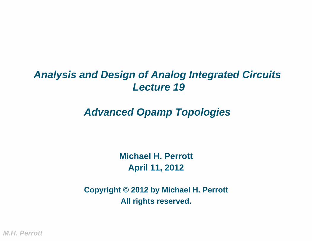
Single-Ended Versus Fully Differential Topologies

Analog circuits are sensitive to noise from the power supply and other coupling mechanisms

Fully differential topologies can offer rejection of common-mode noise (such as from supplies)- Information is encoded as the difference between two

signals- More complex implementation than single-ended

designs3

C1

R1Vin

Vref

Vout

Single-EndedC1a

R1aVin+ Vout+

R1b

Vin- Vout-

C1b

Fully Differential

M.H. Perrott

Key Focus of Lecture

Examine fully differential version of basic two stage opamp

Examine more advanced opamp topologies and the advantages/disadvantages they present

4

M.H. Perrott

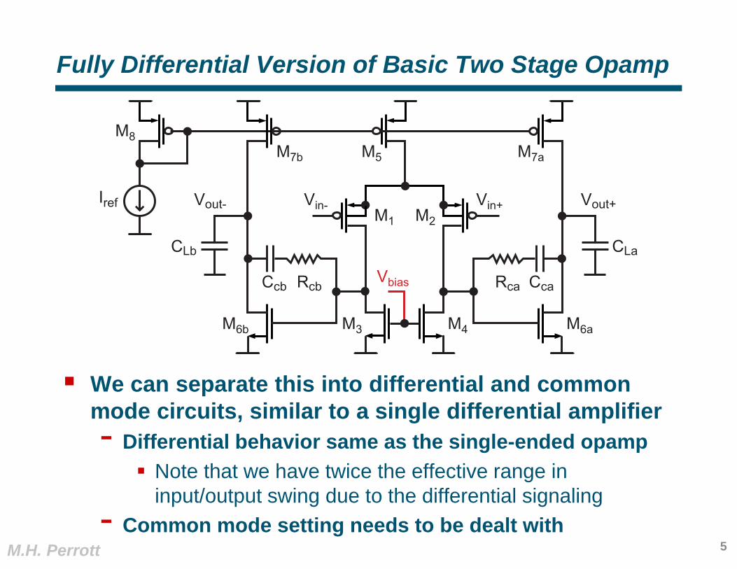
Fully Differential Version of Basic Two Stage Opamp

We can separate this into differential and common mode circuits, similar to a single differential amplifier- Differential behavior same as the single-ended opamp

Note that we have twice the effective range in input/output swing due to the differential signaling

- Common mode setting needs to be dealt with5

M7a

M6a

IrefM1 M2

M3

M8

Vout+

CLa

CcaRca

M4

M5

Vin+Vin-

M7b

M6b

Vout-

CLb

Ccb RcbVbias

M.H. Perrott

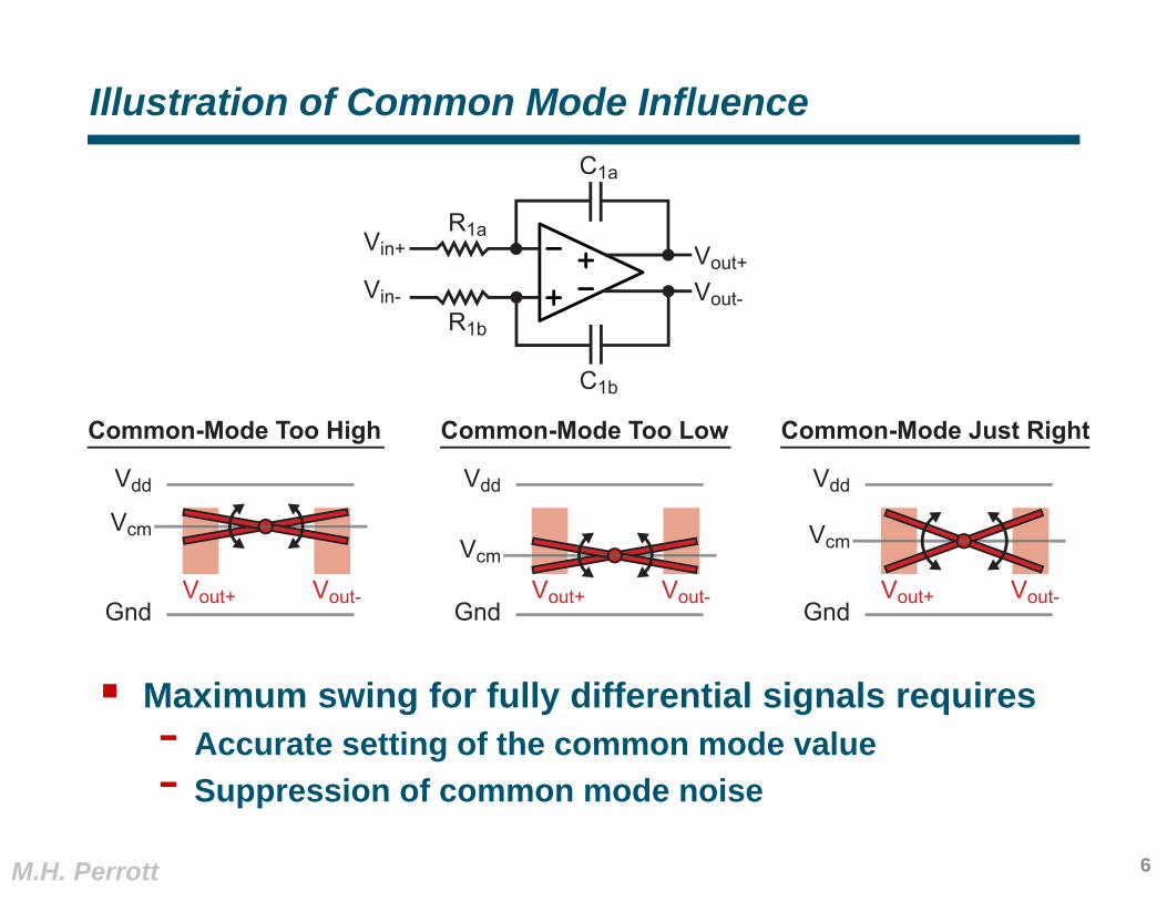
Illustration of Common Mode Influence

Maximum swing for fully differential signals requires- Accurate setting of the common mode value- Suppression of common mode noise

6

C1a

R1aVin+ Vout+

R1b

Vin- Vout-

C1b

Vcm

Vout+ Vout-

Vdd

Gnd

Vcm

Vout+ Vout-

Vdd

Gnd

Vcm

Vout+ Vout-

Vdd

Gnd

Common-Mode Too High Common-Mode Too Low Common-Mode Just Right

M.H. Perrott

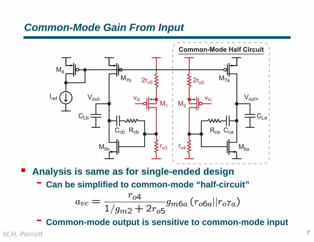
Common-Mode Gain From Input

Analysis is same as for single-ended design- Can be simplified to common-mode “half-circuit”

- Common-mode output is sensitive to common-mode input7

M1 M2

ro3

2ro5 2ro5

ro4

vic vic

M7a

M6a

Iref

M8

Vout+

CLa

CcaRca

M7b

M6b

Vout-

CLb

Ccb Rcb

Common-Mode Half Circuit

avc =ro4

1/gm2 + 2ro5gm6a (ro6a||ro7a)

M.H. Perrott

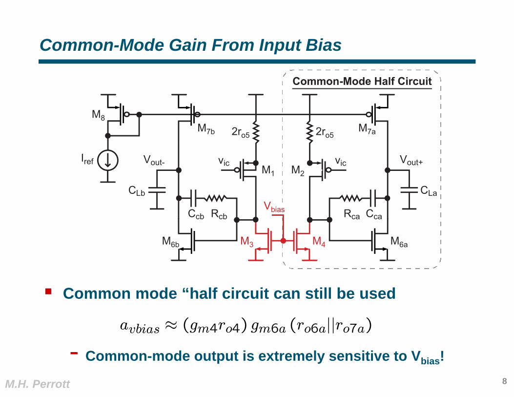
Common-Mode Gain From Input Bias

Common mode “half circuit can still be used

- Common-mode output is extremely sensitive to Vbias!8

M1 M2

2ro5 2ro5

vic vic

M7a

M6a

Iref

M8

Vout+

CLa

CcaRca

M7b

M6b

Vout-

CLb

Ccb Rcb


M3 M4

Vbias

avbias ≈ (gm4ro4) gm6a (ro6a||ro7a)

M.H. Perrott

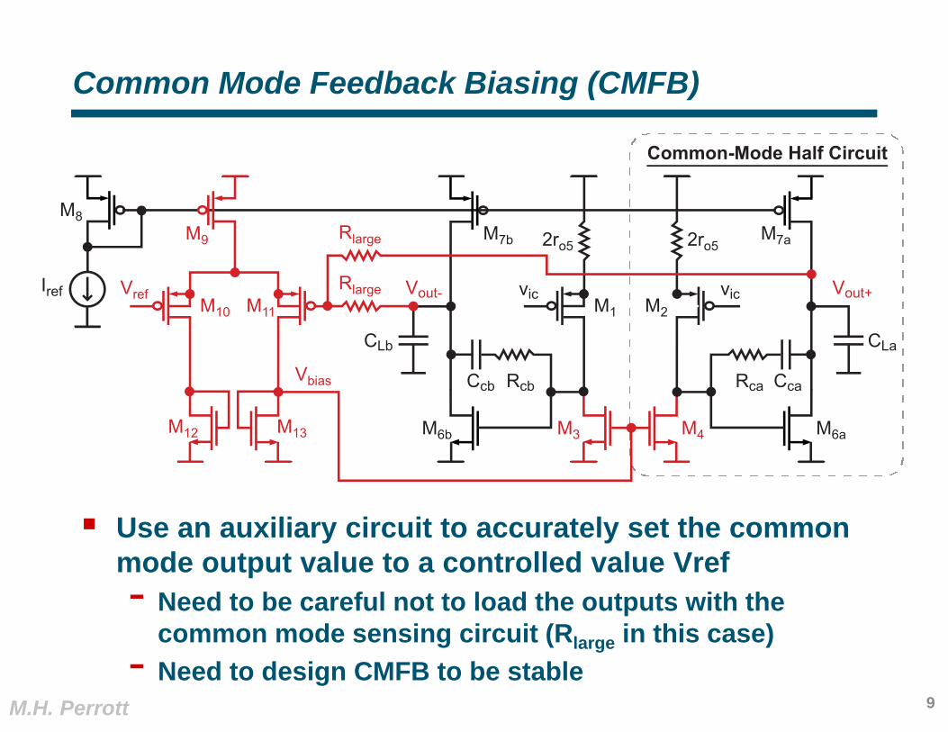
Common Mode Feedback Biasing (CMFB)

Use an auxiliary circuit to accurately set the common mode output value to a controlled value Vref- Need to be careful not to load the outputs with the

common mode sensing circuit (Rlarge in this case)- Need to design CMFB to be stable

9

M1 M2

2ro5 2ro5

vic vic

M7a

M6a

Iref

M8

Vout+

CLa

CcaRca

M7b

M6b

Vout-

CLb

Ccb Rcb


M3 M4

Vbias

M10 M11

M12 M13

M9

RlargeVref

Rlarge

M.H. Perrott

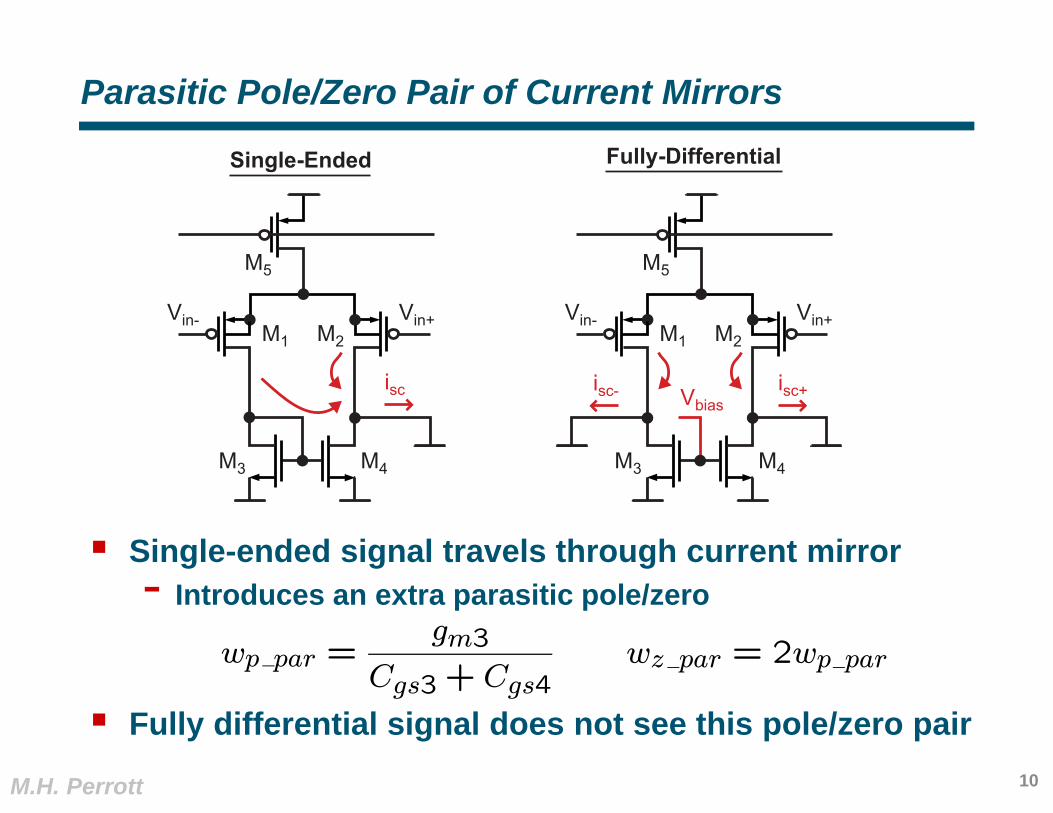
Parasitic Pole/Zero Pair of Current Mirrors

Single-ended signal travels through current mirror- Introduces an extra parasitic pole/zero

Fully differential signal does not see this pole/zero pair10

M1 M2

M4

M5

Vin+Vin-

Vbias

M1 M2

M4

M5

Vin+Vin-

isc

Single-Ended Fully-Differential

M3M3

isc+isc-

wp par =gm3

Cgs3 + Cgs4wz par = 2wp par

M.H. Perrott

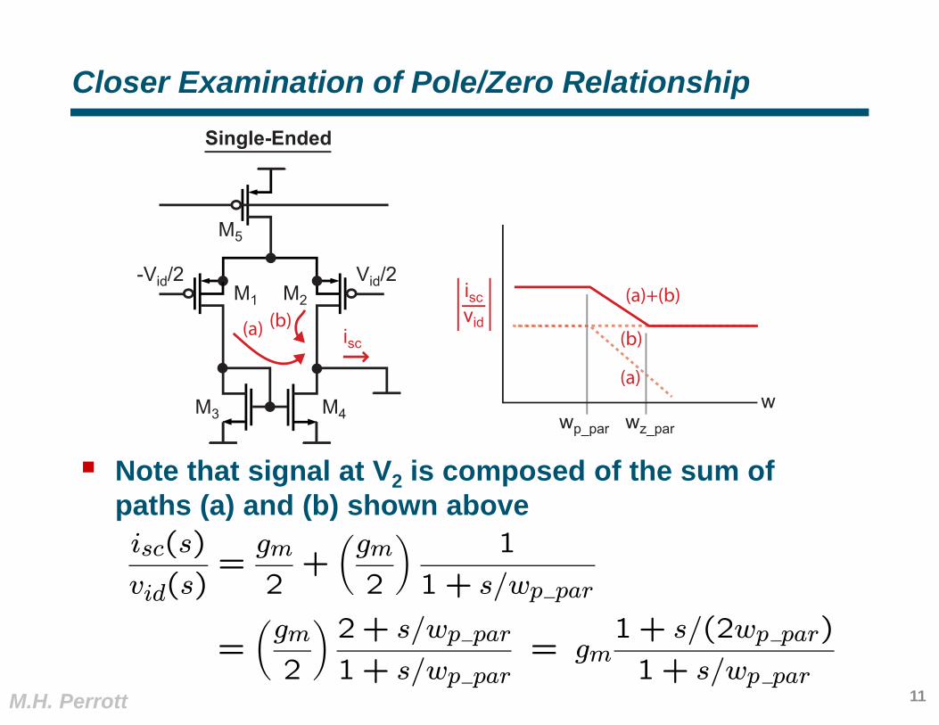
Closer Examination of Pole/Zero Relationship

Note that signal at V2 is composed of the sum of paths (a) and (b) shown above

11

M1 M2

M4

M5

Vid/2-Vid/2

Single-Ended

M3

(a) (b)

(a)

(b)

(a)+(b)

wp_par wz_par

w

iscvid

isc

isc(s)

vid(s)=gm

2+

µgm

2

¶1

1 + s/wp par

=

µgm

2

¶2+ s/wp par

1+ s/wp par= gm

1+ s/(2wp par)

1 + s/wp par

M.H. Perrott

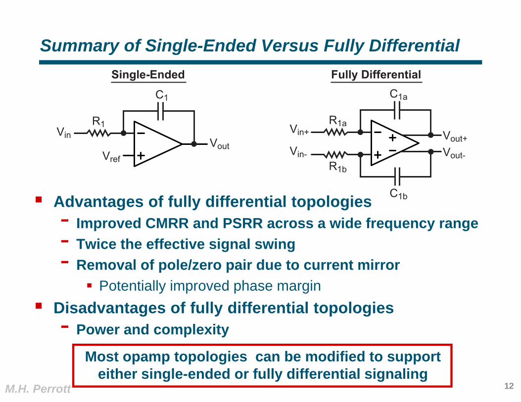
Summary of Single-Ended Versus Fully Differential

Advantages of fully differential topologies- Improved CMRR and PSRR across a wide frequency range- Twice the effective signal swing- Removal of pole/zero pair due to current mirror

Potentially improved phase margin Disadvantages of fully differential topologies

- Power and complexity

12

C1

R1Vin

Vref

Vout

Single-EndedC1a

R1aVin+ Vout+

R1b

Vin- Vout-

C1b

Fully Differential

Most opamp topologies can be modified to supporteither single-ended or fully differential signaling

M.H. Perrott

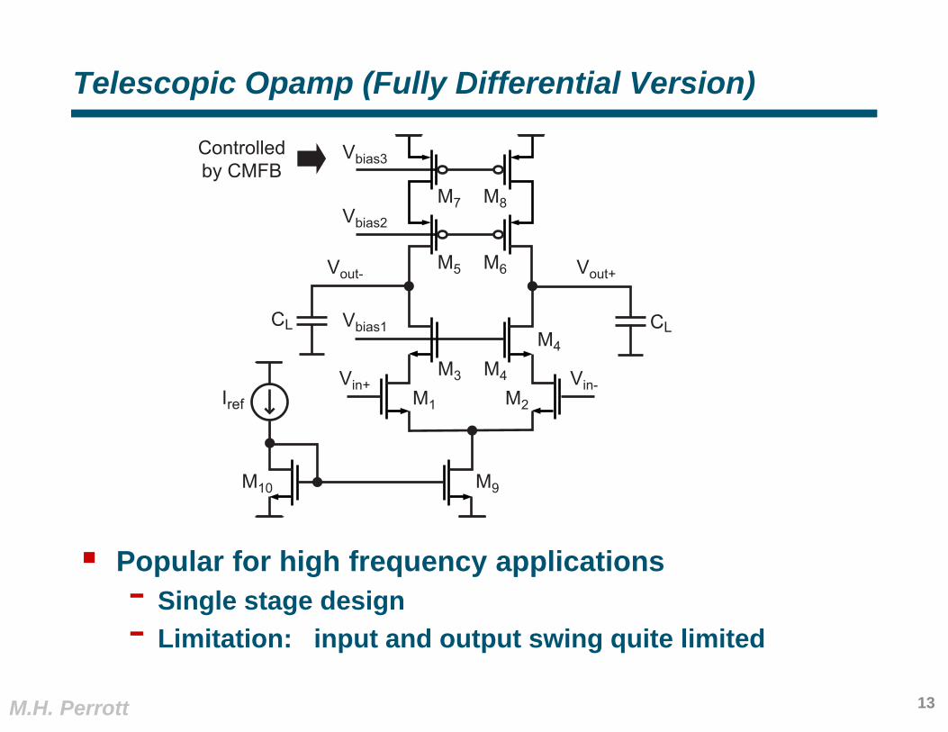
Telescopic Opamp (Fully Differential Version)

Popular for high frequency applications- Single stage design- Limitation: input and output swing quite limited

13

M4

Vin+M3

M1 M2Iref

Vbias1

Vbias2

Vbias3

M4

M5 M6

M7 M8

M9M10

Vin-

CLCL

Vout+Vout-

Controlledby CMFB

M.H. Perrott

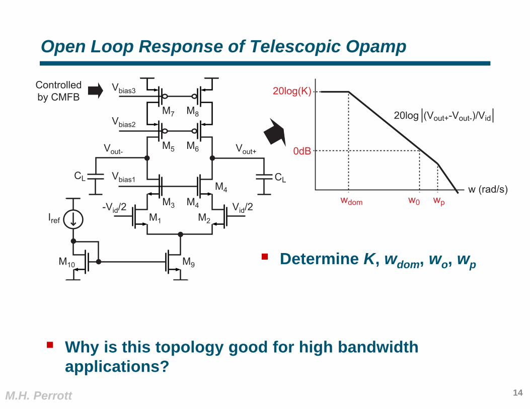
Open Loop Response of Telescopic Opamp

Determine K, wdom, wo, wp

14

M4

M3

M1 M2Iref

Vbias1

Vbias2

Vbias3

M4

M5 M6

M7 M8

M9M10

Vid/2

CLCL

Vout+Vout-

Controlledby CMFB

(Vout+-Vout-)/Vid

w (rad/s)wdom

20log

20log(K)

wp

0dB

w0-Vid/2

Why is this topology good for high bandwidth applications?

M.H. Perrott

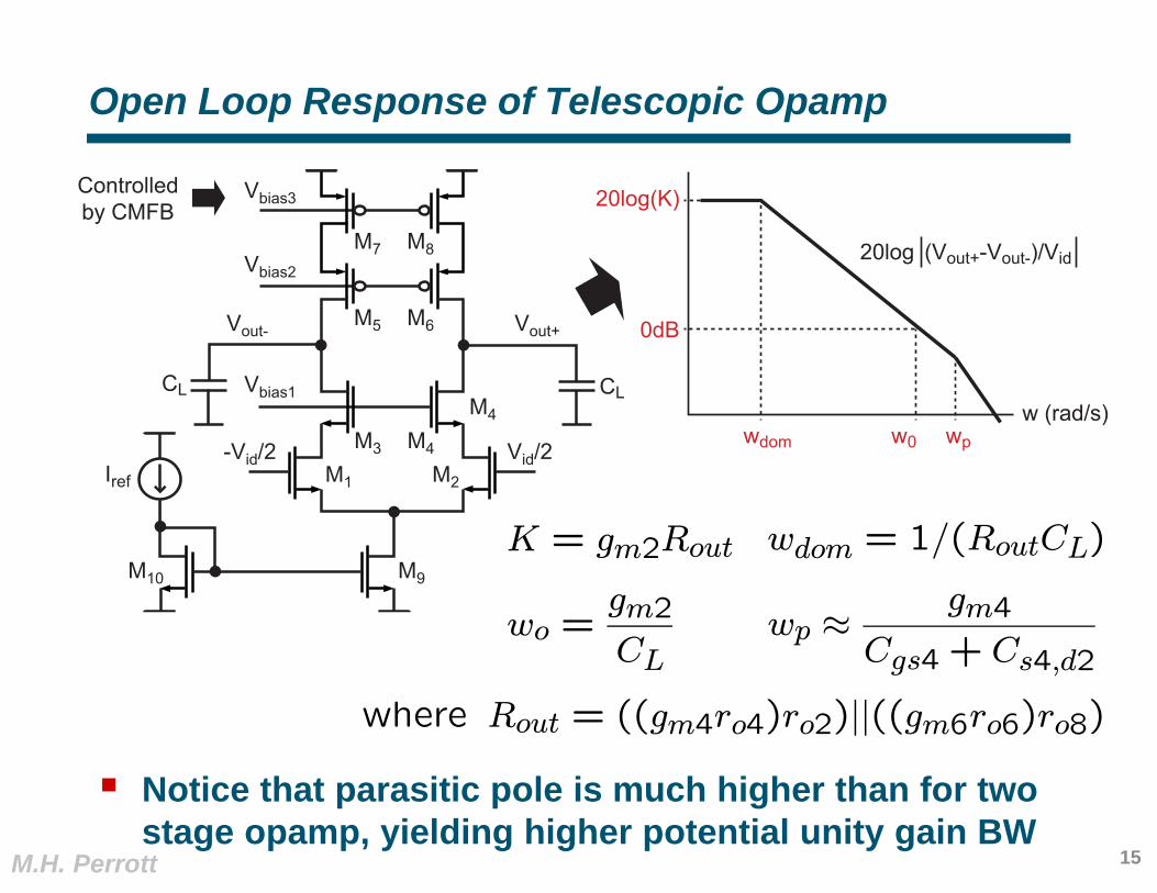
Open Loop Response of Telescopic Opamp

Notice that parasitic pole is much higher than for two stage opamp, yielding higher potential unity gain BW

15

M4

M3

M1 M2Iref

Vbias1

Vbias2

Vbias3

M4

M5 M6

M7 M8

M9M10

Vid/2

CLCL

Vout+Vout-

Controlledby CMFB

(Vout+-Vout-)/Vid

w (rad/s)wdom

20log

20log(K)

wp

0dB

w0-Vid/2

where Rout = ((gm4ro4)ro2)||((gm6ro6)ro8)

wdom = 1/(RoutCL)K = gm2Rout

wo =gm2CL

wp ≈gm4

Cgs4 + Cs4,d2

M.H. Perrott

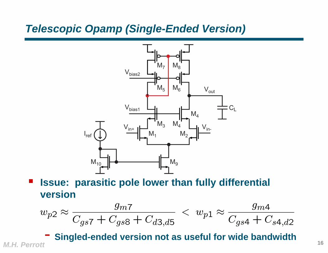
Telescopic Opamp (Single-Ended Version)

Issue: parasitic pole lower than fully differential version

- Singled-ended version not as useful for wide bandwidth16

M4

Vin+M3

M1 M2Iref

Vbias1

Vbias2

M4

M5 M6

M7 M8

M9M10

Vin-

CL

Vout

wp2 ≈gm7

Cgs7 + Cgs8 + Cd3,d5< wp1 ≈

gm4Cgs4 + Cs4,d2

M.H. Perrott

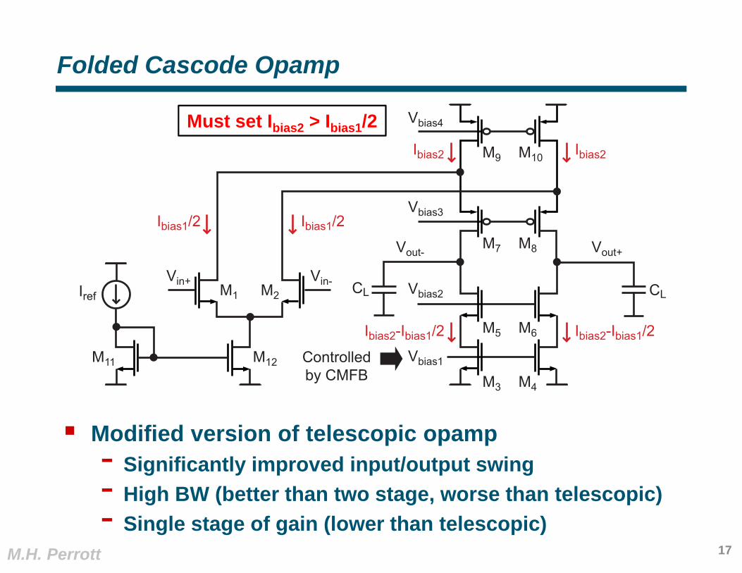
Folded Cascode Opamp

Modified version of telescopic opamp- Significantly improved input/output swing- High BW (better than two stage, worse than telescopic)- Single stage of gain (lower than telescopic)

17

Vbias2

Vbias3

Vbias4

M7 M8

M9 M10

CLCL

Vout+Vout-

Controlledby CMFB

M1 M2Iref

M12M11

Vin-Vin+

Vbias1

M5 M6

M3 M4

Ibias1/2 Ibias1/2

Ibias2 Ibias2

Ibias2-Ibias1/2Ibias2-Ibias1/2

Must set Ibias2 > Ibias1/2

M.H. Perrott

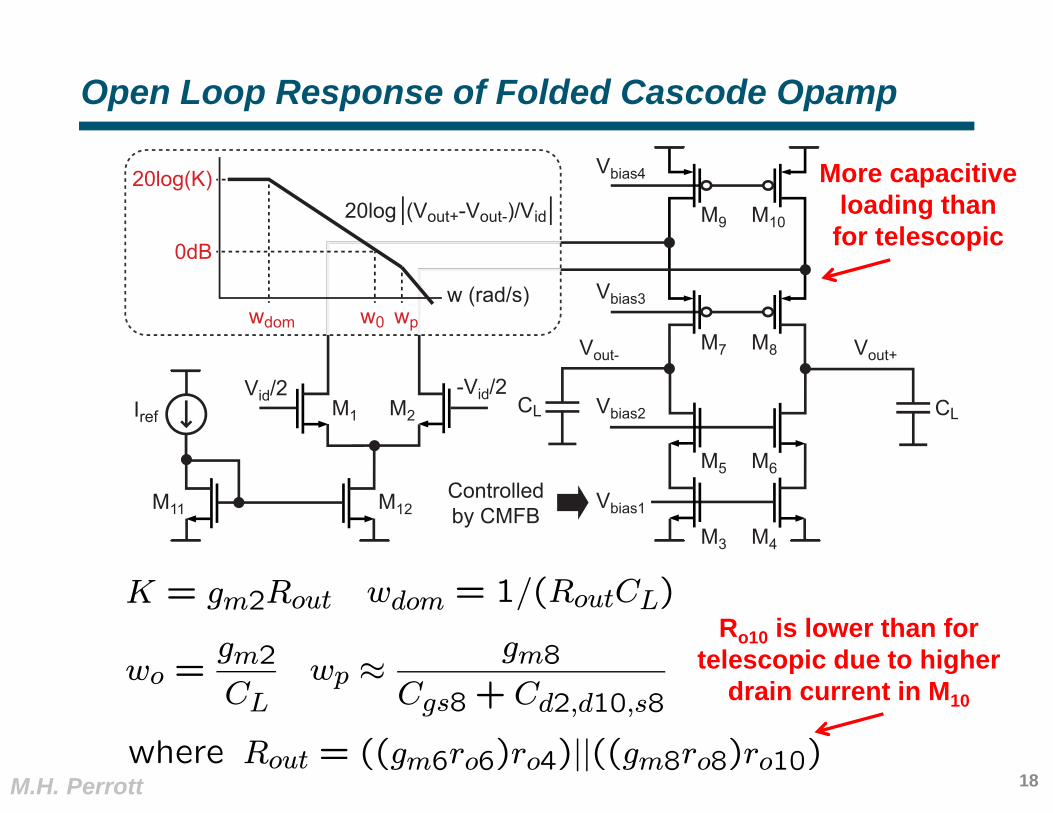
Open Loop Response of Folded Cascode Opamp

18

Vbias2

Vbias3

Vbias4

M7 M8

M9 M10

CLCL

Vout+Vout-

Controlledby CMFB

M1 M2Iref

M12M11

Vid/2

Vbias1

M5 M6

M3 M4

-Vid/2

(Vout+-Vout-)/Vid

w (rad/s)wdom

20log20log(K)

wp

0dB

w0


wdom = 1/(RoutCL)K = gm2Rout

wo =gm2CL

wp ≈gm8

Cgs8 + Cd2,d10,s8

Ro10 is lower than fortelescopic due to higher

drain current in M10

More capacitiveloading than

for telescopic

M.H. Perrott

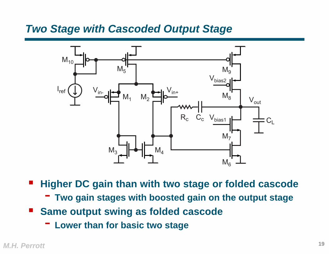
Two Stage with Cascoded Output Stage

Higher DC gain than with two stage or folded cascode- Two gain stages with boosted gain on the output stage

Same output swing as folded cascode- Lower than for basic two stage

19

Vbias2

M8

M9

CL

Vout

Vbias1

M7

M6

IrefM1 M2

M3

M10

CcRc

M4

M5

Vin+Vin-

M.H. Perrott

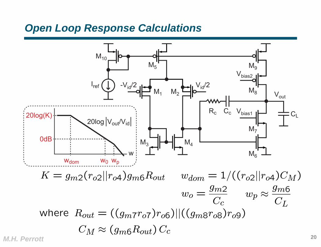
Open Loop Response Calculations

20

Vbias2

M8

M9

CL

Vout

Vbias1

M7

M6

IrefM1 M2

M3

M10

CcRc

M4

M5

Vid/2

Vout/Vid

wwdom

20log20log(K)

wp

0dB

w0

-Vid/2


wdom = 1/((ro2||ro4)CM)K = gm2(ro2||ro4)gm6Routwo =

gm2Cc

wp ≈gm6CL

CM ≈ (gm6Rout)Cc

M.H. Perrott

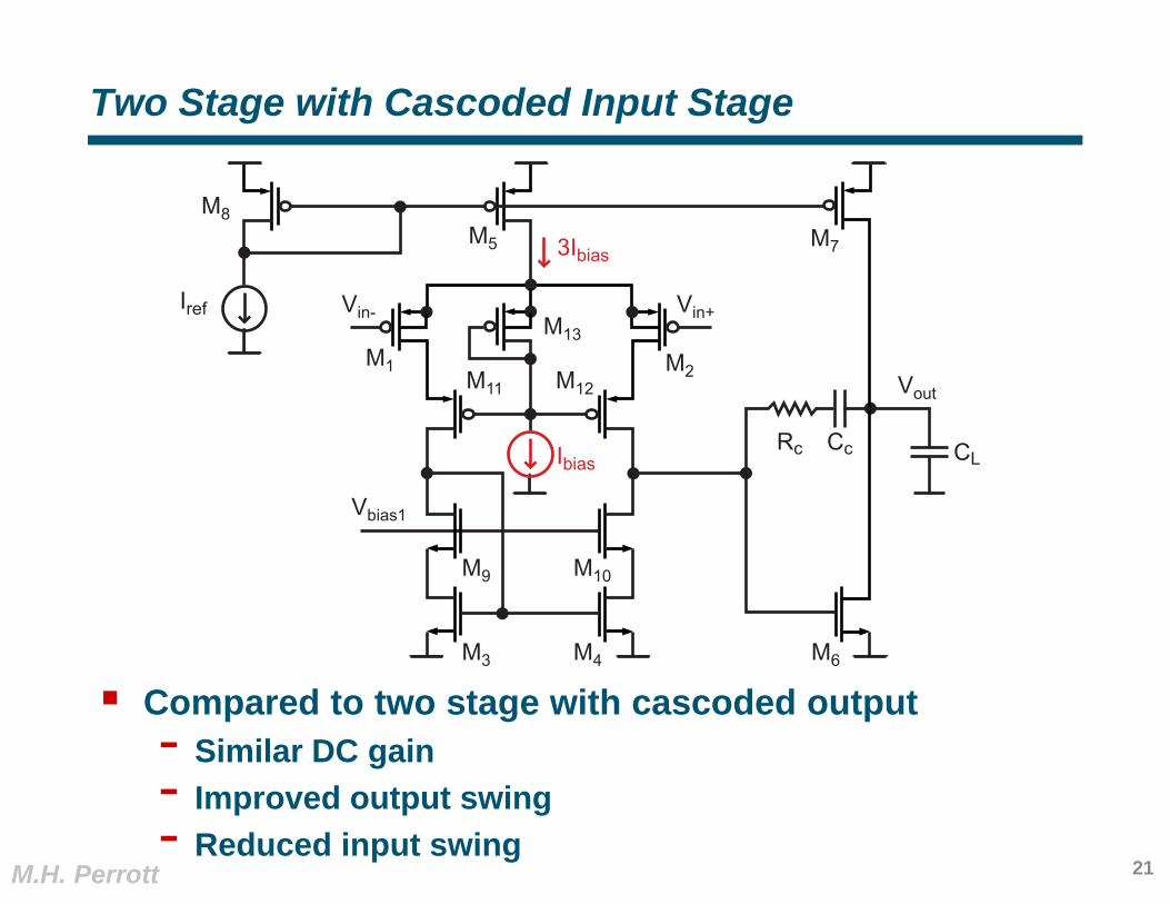
Two Stage with Cascoded Input Stage

Compared to two stage with cascoded output- Similar DC gain- Improved output swing- Reduced input swing

21

M7

CL

Vout

M6

Iref

M1 M2

M8

CcRc

M5

Vin+Vin-

Vbias1

M11 M12

M9 M10

M3 M4

3Ibias

M13

Ibias

M.H. Perrott

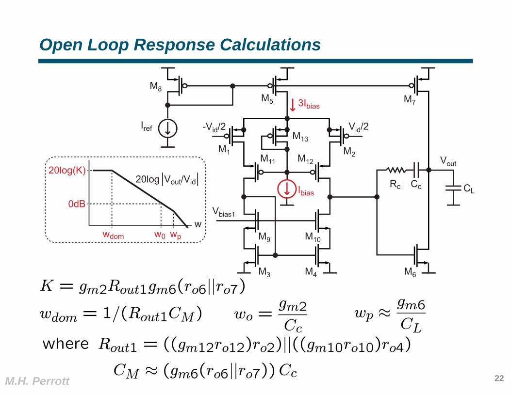
Open Loop Response Calculations

22

M7

CL

Vout

M6

Iref

M1 M2

M8

CcRc

M5

-Vid/2

Vbias1

M11 M12

M9 M10

M3 M4

3Ibias

M13

Ibias

Vout/Vid

wwdom

20log20log(K)

wp

0dB

w0

Vid/2

where Rout1 = ((gm12ro12)ro2)||((gm10ro10)ro4)wdom = 1/(Rout1CM)

K = gm2Rout1gm6(ro6||ro7)wo =

gm2Cc

wp ≈gm6CL

CM ≈ (gm6(ro6||ro7))Cc

M.H. Perrott 23

Summary

Opamp topologies can be configured to process fully differential signals- Provides improved immunity to noise from common-mode

perturbations such as power supply noise- Increases effective signal swing by a factor of two- Carries additional complexity for CMFB and increased

power consumption Integrated opamps are often custom designed for a

given application- Each application places different demands on DC gain,

bandwidth, signal swing, etc.- Opamp topologies considered today include telescopic,

folded cascode, and modified two stage Each carries different tradeoffs on the above specifications

Documents

Advanced Opamp Topologies - CppSim · M.H. Perrott Summary of Single-Ended Versus Fully Differential Advantages of fully differential topologies-Improved CMRR and PSRR across a wide