Advanced Sensor and Dynamics Models with an Application to

1

Advanced Sensor and Dynamics Models with an Application to Sensor Management

Wolfgang Koch German Defence Research Establishment (FGAN e.V.)

Germany

1. Introduction

The methods provided by sensor and data fusion [14] are important tools for fusing large sets of mutually complementary data end efficiently exploiting the sensor systems available. A challenging exploitation technology at the common interface between sensors, command & control systems, and the human decision makers involved, this technology plays a key role in applications with time-critical situations or in situations with a high decision risk, where human deficiencies are to be compensated by automatically or interactively working fusion techniques (compensating decreasing attention in routine situations, focusing the attention on anomalous or rare events, complementing limited memory, reaction, or combination capabilities of human beings). Besides the advantages of reducing the human work load in routine or mass tasks, data fusion from mutually complementary information sources can well produce qualitatively new knowledge that otherwise would remain unrevealed.

A. Providing Elements for Situation Pictures

Sensor and data fusion provides ‘information elements’ for producing near real-time situation pictures, which electronically represent a complex and dynamically evolving overall scenario in the air, on the ground, at sea, or in an urban environment. The concrete operational requirements in a given application define the particular information sources to be fused. A careful analysis of the underlying requirements is thus essential for any fusion system design. Information elements are extracted from currently received sensor data while taking into account the available context knowledge and pre-history. They typically provide answers to questions related to objects of interest such as: Do objects exist at all, and how many of them are in the sensors’ fields of view? Where are they at what time? Where will they be in the future with what probability? How can their overall behavior be characterized? Are anomalies or hints about their possible intentions recognizable? What can be inferred about the classes the objects belong to or even their identities? Are there characteristic interrelations between individual objects? In which regions do they have their origin? What can be said about their possible destinations? Are object flows visible? Where are sources or sinks of traffic? The sensor data to be fused can be inaccurate, incomplete, or ambiguous. Closely-spaced objects are often totally or partially unresolvable. Possibly, the measured object parameters O

pen

Acc

ess

Dat

abas

e w

ww

.inte

chw

eb.o

rg

Source: Sensor and Data Fusion, Book edited by: Dr. ir. Nada Milisavljević, ISBN 978-3-902613-52-3, pp. 490, February 2009, I-Tech, Vienna, Austria

www.intechopen.com

Sensor and Data Fusion

2

are false or corrupted by hostile measures. The context information is in many cases hard to be formalized or even contradictory. These deficiencies of the information to be fused are unavoidable in any real-world application. Therefore, the extraction of ‘information elements’ for situation pictures is by no means trivial.

B. Aspects of Sensor and Data Fusion

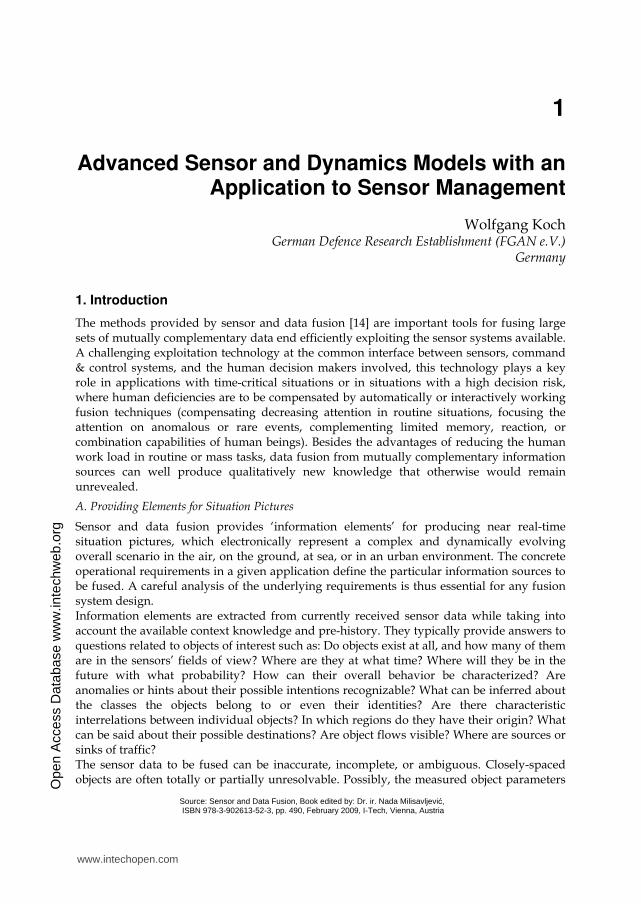
Among the primary technical prerequisites for sensor data and information fusion are communication links with a sufficient bandwidth, small latency, and robustness against failure or jamming. Moreover, the transformation of the sensor data into a common coordinate system requires a precise space-time registration of the sensors, including their mutual alignment. Figure 1 provides an overview of different aspects and their mutual interrelation. The

sensors play a central role and can be located in different ways (collocated, distributed,

mobile) producing measurements of the same or of a different type. Fusion of

heterogeneous sensor data is of particular importance, such as the combination of kinematic

measurements with measured attributes providing information on the classes to which

objects belongs to. In the context of defense and security applications especially, the

distinction between active and passive sensing is important since passive sensors enable

covert surveillance, which does not reveal itself by emitting radiation. Multifunctional

sensor systems offer additional operational modes, thus requiring more intelligent strategies

of sensor management that provide feedback via control or correction commands to the

process of information acquisition. By this the surveillance objectives can often be reached

more efficiently. Context information is given, for example, by available knowledge on the

sensor and object properties, which is often quantitatively described by statistical models.

Context knowledge is also environmental information on roads or topographical occlusions

(GIS: Geographical Information Systems). Seen from a different perspective, context

information, such as road maps, can be extracted from real-time sensor data as well [27].

Militarily relevant context knowledge (e.g. doctrines, planning data, tactics) and human

observer reports (HUMINT: Human Intelligence) is also important information in the fusion

process [4]. The exploitation of context information of any kind can significantly improve

the fusion system performance.

Fig. 1. Sensor data and information fusion for situation pictures: overview of characteristic aspects and their mutual interrelation.

www.intechopen.com


3

The information elements required for producing a timely situation picture are provided by an integrative, spatio-temporal processing of the various pieces of information available, which in themselves often have only limited value for understanding the situation. Essentially, within the fusion process logical cross-references, inherent complementarity, and redundancy are exploited. More concretely speaking, the methods used are characterized by a stochastic approach (estimating relevant state quantities) and a more heuristically defined knowledgebased approach (imitating the actual human behavior when exploiting information). Besides the operational requirements, this more or less coherent methodology is the second building principle, which gives the field of sensor data and information fusion its characteristic shape.

C. Overview of a Generic Tracking System

Among the fusion products, so-called ‘tracks’ are of particular importance. Tracks represent knowledge on relevant state quantities of individual objects, object groups such as convoys and formations, or even large object aggregations (e.g. march columns). The information obtained by ‘tracking’ [6], [2], [22] includes in particular the history of the objects. If possible, a one-toone association between the objects/object groups and the tracks is to be established and has to be preserved as long as possible (track continuity). Quantitative measures describing the quality of this knowledge are important constituents of tracks. The achievable track quality, however, does not only depend on the sensor performance, but also on the operational conditions within the actually considered scenario and the available context knowledge.

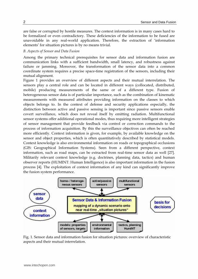
Fig. 2. Generic scheme of functional building blocks within a tracking/fusion system along with its relation to the sensors (centralized configuration, type IV according to O. Drummond).

Figure 2 shows a generic scheme of functional building blocks within a tracking/fusion system along with its relation to the underlying sensors. After passing a detection process, essentially working as a means of data rate reduction, the signal processing provides

www.intechopen.com


4

estimates of parameters characterizing the waveforms received at the sensors’ front ends (e.g. radar antennas). From these estimates sensor reports are created, i.e. measured quantities possibly related to objects of interest, which are the input for the tracking/fusion system. All sensor data that can be associated to existing tracks are used for track maintenance (using, e.g., prediction, filtering, and retrodiction). The remaining data are processed for initiating new tentative tracks (multiple frame track extraction). Association techniques thus play a key role in tracking/fusion applications. Context information in terms of statistical models (sensor performance, object characteristics, object environment) is a prerequisite to track maintenance and initiation. Track confirmation/termination, classification/identification, and fusion of tracks related to the same objects or object groups is part of the track processing. The scheme is completed by a manmachine interface with displaying and interaction functions. Context information can be updated or modified by direct human interaction or by the track processor itself, for example as a consequence of object classification or road map extraction. In the case of multifunctional sensors, feedback exists from the tracking system to the process of sensor data acquisition (sensor management).

D. A Characteristic Application: Sensor Management

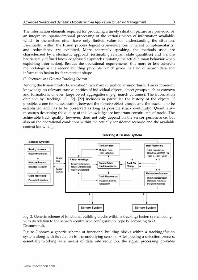
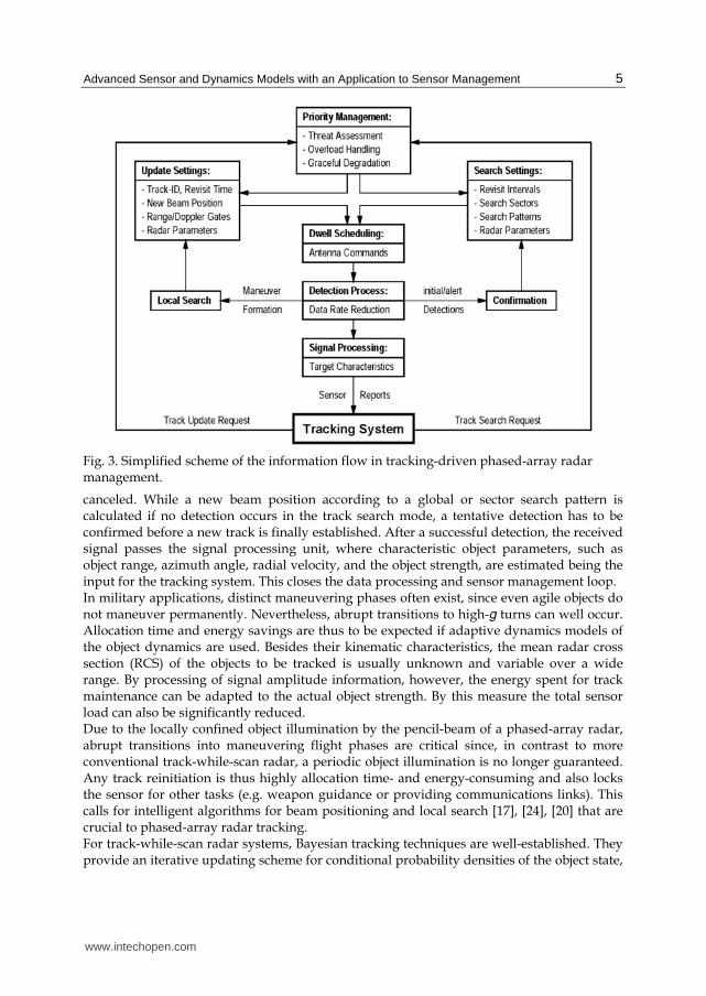
Modern multifunctional agile-beam radar based on phased-array technology is an excellent example for a sensor system that requires sophisticated sensor management algorithms. This is particularly true for multiple object tracking tasks where such systems call for algorithms that efficiently exploit their degrees of freedom, which are variable over a wide range and may be chosen individually for each track. Of special interest are military air situations where both agile objects and objects significantly differing in their radar cross section must be taken into account. Unless properly handled, such situations can be highly allocation time- and energyconsuming. In this context, advanced sensor and dynamics models for combined tracking and sensor management are discussed, i.e. control of data innovation intervals, radar beam positioning, and transmitted energy management. By efficiently exploiting its limited resources, the total surveillance performance of the sensor system can be much improved. Figure 3 shows a simplified scheme illustrating the information flow in tracking-driven phasedarray radar management. The starting point is the tracking system, which generates a request for new sensor information based on the current quality of an already established individual object track or on the requirement of initiating new tracks. We thus distinguish between track update and search requests, which enter into the priority management unit where its rank is evaluated based on the current threat or overload situation, for example, thus enabling graceful system degradation when necessary. For each preparation of a radar system allocation, track-specific radar parameters must be set, such as the calculated radar revisit time and the corresponding radar beam position, rangeand Doppler-gates, or the type of the radar wave forms to be transmitted. Track search requests require the setting of appropriate revisit intervals, search sectors and patterns, and other radar parameters. In the dwell scheduling unit these preparations are transformed into antenna commands, by which the radar sensor is allocated and radar energy transmitted. The received echo signals pass a detection unit. If no detection occurs in the track maintenance mode, a local search procedure is initiated, new radar parameters are set, and a subsequent radar sensor allocation is started with as small a time delay as possible. This local search loop is repeated until either a valid detection is produced or the track is

www.intechopen.com


5

Fig. 3. Simplified scheme of the information flow in tracking-driven phased-array radar management.

canceled. While a new beam position according to a global or sector search pattern is calculated if no detection occurs in the track search mode, a tentative detection has to be confirmed before a new track is finally established. After a successful detection, the received signal passes the signal processing unit, where characteristic object parameters, such as object range, azimuth angle, radial velocity, and the object strength, are estimated being the input for the tracking system. This closes the data processing and sensor management loop. In military applications, distinct maneuvering phases often exist, since even agile objects do not maneuver permanently. Nevertheless, abrupt transitions to high-g turns can well occur. Allocation time and energy savings are thus to be expected if adaptive dynamics models of the object dynamics are used. Besides their kinematic characteristics, the mean radar cross section (RCS) of the objects to be tracked is usually unknown and variable over a wide range. By processing of signal amplitude information, however, the energy spent for track maintenance can be adapted to the actual object strength. By this measure the total sensor load can also be significantly reduced. Due to the locally confined object illumination by the pencil-beam of a phased-array radar, abrupt transitions into maneuvering flight phases are critical since, in contrast to more conventional track-while-scan radar, a periodic object illumination is no longer guaranteed. Any track reinitiation is thus highly allocation time- and energy-consuming and also locks the sensor for other tasks (e.g. weapon guidance or providing communications links). This calls for intelligent algorithms for beam positioning and local search [17], [24], [20] that are crucial to phased-array radar tracking. For track-while-scan radar systems, Bayesian tracking techniques are well-established. They provide an iterative updating scheme for conditional probability densities of the object state,

www.intechopen.com


6

given all sensor data and a priori information available. In those applications data acquisition and tracking are completely decoupled. For phased-array radar, however, the current signal-to-noise ratio of the object (i.e. the detection probability) strongly depends on the correct positioning of the pencil-beam, which is now taken into the responsibility of the tracking system. Sensor control and data processing are thus closely interrelated. This basically local character of the tracking process constitutes the principal difference between phased-array and track-while-scan applications from a tracking point of view. By using suitable sensor models, however, this fact can be incorporated into the Bayesian formalism. The potential of this approach is thus also available for phased-array radar. The more difficult problem of global optimization, taking successive allocations into account, is not addressed here.

2. Sensor and dynamics models in bayesian object tracking

Fusing data produced at different instants of time, i.e. the tracking problem, is typically characterized by uncertainty and ambiguities, which are inherent in the underlying scenario, the object dynamics, and the sensors used. The Bayesian approach provides a well-suited methodology for dealing with many of these phenomena. More concretely speaking, the Bayesian approach provides a processing scheme for dealing with uncertain information (of a particular type), which also allows to make ‘delayed’ decisions if a unique decision cannot be made in a particular data situation. Ambiguities can have different causes: Sensors may produce ambiguous data due to their limited resolution capabilities or due to phenomena such as Doppler blindness in MTI radar (MTI: Moving Target Indicator). Often the objects’ environment is a source of ambiguities itself (dense object situations, residual clutter, man-made noise, unwanted objects). A more indirect type of ambiguities arises from the objects’ behavior (e.g. qualitatively distinct maneuvering phases). Finally, the context knowledge to be exploited can imply problem-inherent ambiguities as well, such as intersections in road maps or ambiguous tactical rules describing the over-all object behavior. The general multiple-object, multiple-sensor tracking task, however, is highly complex and involves sophisticated combinatorial considerations that are beyond the scope of this chapter (see [5], [30] as an introduction). Nevertheless, in many applications, the tracking task can be partitioned into independent sub-problems of (much) less complexity. According to this discussion, we proceed along the following lines.

• Basis: In the course of time, one or several sensors produce measurements of one or more objects of interest. The accumulated sensor data are an example of a ‘time series’. Each object is characterized by its current ‘state’, a vector typically consisting of the current object position, its velocity, and acceleration.

• Objective: Learn as much as possible about the individual object states at each time of interest by analyzing the ‘time series’ created by the sensor data.

• Problem: The sensor information is inaccurate, incomplete, and possibly even ambiguous. Moreover, the objects’ temporal evolution is usually not well-known.

• Approach: Interpret sensor measurements and object state vectors as random variables. Describe by probability density functions (pdfs) what is known about these random variables.

• Solution: Derive iteration formulae for calculating the probability density functions of the state variables and develop a mechanism for initiating the iteration. Derive state estimates from the pdfs along with appropriate quality measures.

www.intechopen.com


7

A. The Key-role of Bayes’ Formula

At particular instants of time denoted by tl, l = 1, ..., k, we consider the set Zl =

of nl measurements related to the object state xl. In case of multiple objects xl is the joint state.

The corresponding time series up to and including tk is recursively defined by k = {Zk, nk,

k-1}. The central question of object tracking is: What can be known about the object states xl

at time instants tl, i.e. for the past (l < k), at present (l = k), and in the future (l > k), by

exploiting the sensor data collected in the times series k? According to the approach previously sketched, the answer is given by the conditional probability density functions

(pdf) p(xl│ k) to be calculated iteratively as a consequence of Bayes’ rule. For l = k, i.e. for object states at the current time tk, we obtain:

(1)

In other words, p(xk│ k) can be calculated from the pdfs p(xk│ k-1) and p(Zk, nk│xk).

p(xk│ k-1) describes, what is known on xk given all past sensor data k-1, i.e. a prediction. Obviously, p(Zk, nk│xk) needs to be known up to a constant factor only. Any function

(2)

produces the same result. Functions of this type are also called likelihood functions and

describe what can be learned from the current sensor output Zk, nk about the object state xk at

this time. This is the reason, why likelihood functions are often also called “sensor models”,

since they mathematically represent the sensor, its measurements and properties, in the data

processing formalism. For well-separated objects, perfect detection, in absence of false

returns, and for bias-free measurements of linear functions Hkxk of the object state with a

Gaussian, white noise measurement error characterized by a covariance matrix Rk, the

likelihood functions are proportional to a Gaussian: ℓ(xk; zk, Hk, Rk) ∝N(zk; Hkxk, Rk).

B. Prediction Update Step

The pdf p(xk│ k-1) in the Equation 1 is a prediction of the knowledge on the object state for

the time tk based on all the measurements received up to and including time tk-1. By writing

this pdf as a marginal density, p(xk│ k-1) = ∫dxk-1 p(xk, xk-1│ k-1), the object state xk-1 at the

previous time tk-1 comes into play yielding:

(3)

The state transition density p(xk│xk-1, k-1) is often called the “object dynamics model” and

mathematically represents the kinematic object properties in the data processing formalism in the same way as the likelihood function represents the sensor(s). 1) Gauss-Markov Dynamics: A Gauss-Markov dynamics, defined by the transition density

(4)

www.intechopen.com


8

is characterized by the modeling parameters Fk│k-1 (evolution matrix), describing the deterministic part of the temporal evolution, and Dk│k-1 (dynamics covariance matrix), characterizing its stochastic part. If we additionally assume that the previous posterior is a Gaussian, given by

(5)

p(xk│ k-1) is also a Gaussian:

(6)

with an expectation vector x k│k-1 and a covariance matrix Pk│k-1 given by:

(7)

(8)

This directly results from a useful product formula for Gaussians1:

(9)

where we used the abbreviations:

(10)

Note that after applying this formula the integration variable xk-1 in the Equation 3 is no longer contained in the first Gaussian of the product. The integration becomes thus trivial as pdfs are normalized. 2) IMM Dynamics Model: In practical applications, it might be uncertain which dynamics model out of a set of possible alternatives is currently in effect. Such cases, e.g. objects characterized by different modes of dynamical behavior, can be handled by multiple dynamics models with a given probability of switching between them (IMM: Interacting Multiple Models, [2], [6] and the literature cited therein). The model transition probabilities are thus part of the modeling assumptions. More strictly speaking, suppose that r models are given and let jk be denoting the dynamics model assumed to be in effect at time tk, the statistical properties of systems with Markovian switching coefficients are summarized by the following equation:

(11)

1Sketch of proof: Interpret N(z; Hx, R)N(x; y, P) as a joint density p(z, x) = p(z│x)p(x). It can

be written as a Gaussian, from which the marginal and conditional densities p(z), p(x│z) can be derived. In the calculations make use of known formulae for the inverse of a partitioned matrix (see [2, p. 22], e.g.). From p(z, x) = p(x│z)p(z) the formula results.

www.intechopen.com


9

(12)

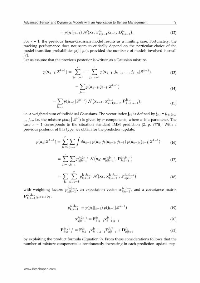
For r = 1, the previous linear-Gaussian model results as a limiting case. Fortunately, the tracking performance does not seem to critically depend on the particular choice of the model transition probabilities p(jk│jk-1), provided the number r of models involved is small [7]. Let us assume that the previous posterior is written as a Gaussian mixture,

(13)

(14)

(15)

i.e. a weighted sum of individual Gaussians. The vector index jk-1 is defined by jk-1 = jk-1, jk-2,

..., jk-n, i.e. the mixture p(xk-1│ k-1) is given by rn components, where n is a parameter. The

case n = 1 corresponds to the situation standard IMM prediction [2, p. ???ff]. With a

previous posterior of this type, we obtain for the prediction update:

(16)

(17)

(18)

with weighting factors

, an expectation vector , and a covariance matrix

given by:

(19)

(20)

(21)

by exploiting the product formula (Equation 9). From these considerations follows that the number of mixture components is continuously increasing in each prediction update step.

www.intechopen.com


10

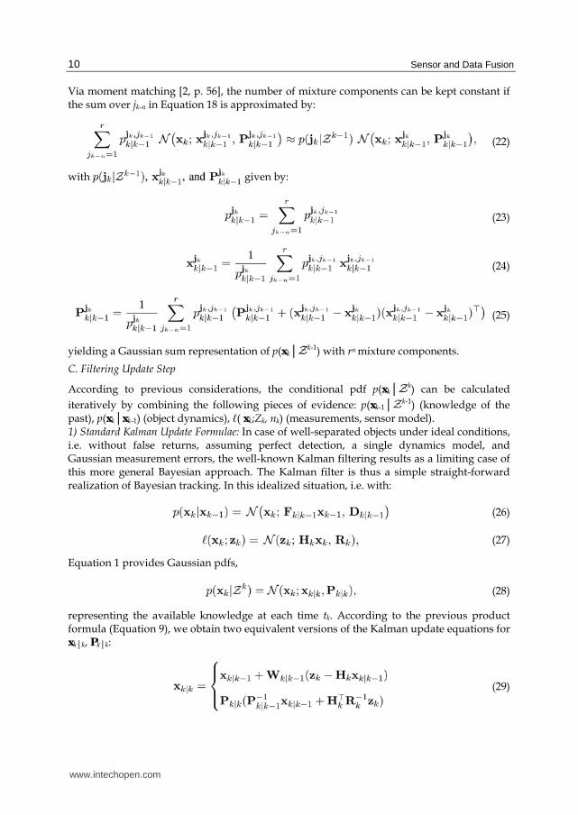
Via moment matching [2, p. 56], the number of mixture components can be kept constant if the sum over jk-n in Equation 18 is approximated by:

(22)

with given by:

(23)

(24)

(25)

yielding a Gaussian sum representation of p(xk│ k-1) with rn mixture components.

C. Filtering Update Step

According to previous considerations, the conditional pdf p(xk│ k) can be calculated

iteratively by combining the following pieces of evidence: p(xk-1│ k-1) (knowledge of the past), p(xk│xk-1) (object dynamics), ℓ( xk;Zk, nk) (measurements, sensor model). 1) Standard Kalman Update Formulae: In case of well-separated objects under ideal conditions, i.e. without false returns, assuming perfect detection, a single dynamics model, and Gaussian measurement errors, the well-known Kalman filtering results as a limiting case of this more general Bayesian approach. The Kalman filter is thus a simple straight-forward realization of Bayesian tracking. In this idealized situation, i.e. with:

(26)

(27)

Equation 1 provides Gaussian pdfs,

(28)

representing the available knowledge at each time tk. According to the previous product formula (Equation 9), we obtain two equivalent versions of the Kalman update equations for xk│k, Pk│k:

(29)

www.intechopen.com


11

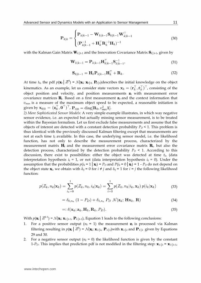
(30)

with the Kalman Gain Matrix Wk│k-1 and the Innovation Covariance Matrix Sk│k-1, given by

(31)

(32)

At time t0, the pdf p(x0│ 0) = N(x0; x0│0, P0│0)describes the initial knowledge on the object

kinematics. As an example, let us consider state vectors , consisting of the

object position and velocity, and position measurements zk with measurement error covariance matrices Rk. Based on a first measurement z0 and the context information that vmax is a measure of the maximum object speed to be expected, a reasonable initiation is

given by , .

2) More Sophisticated Sensor Models: A very simple example illustrates, in which way negative sensor evidence, i.e. an expected but actually missing sensor measurement, is to be treated within the Bayesian formalism. Let us first exclude false measurements and assume that the objects of interest are detected with a constant detection probability PD < 1. This problem is thus identical with the previously discussed Kalman filtering except that measurements are not at each time tk available. In this case, the underlying sensor model, i.e. the likelihood function, has not only to describe the measurement process, characterized by the measurement matrix Hk and the measurement error covariance matrix Rk, but also the detection process, characterized by the detection probability PD < 1. According to this discussion, there exist to possibilities: either the object was detected at time tk, (data interpretation hypothesis ik = 1, or not (data interpretation hypothesis ik = 0). Under the assumption that the probabilities p(ik = 1│xk) = PD and P(ik = 0│xk) = 1 - PD do not depend on the object state xk, we obtain with ij = 0 for i ≠ j and ij = 1 for i = j the following likelihood function:

(33)

(34)

(35)

With p(xk│ k-1) = N(xk; x k│k-1, P k│k-1), Equation 1 leads to the following conclusions:

1. For a positive sensor output (nk = 1) the measurement zk is processed via Kalman

filtering resulting in p(xk│ k) = N(xk; x k│k, P k│k)with x k│k and P k│k given by Equations

29 and 30. 2. For a negative sensor output (nk = 0) the likelihood function is given by the constant

1-PD. This implies that prediction pdf is not modified in the filtering step: x k│k = x k│k-1,

www.intechopen.com


12

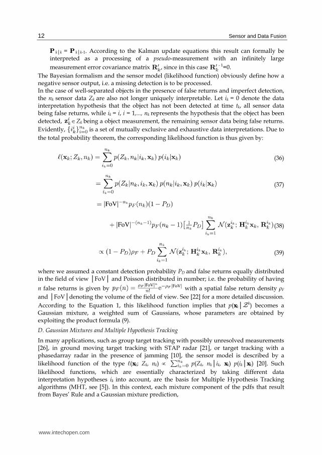
P k│k = P k│k-1. According to the Kalman update equations this result can formally be interpreted as a processing of a pseudo-measurement with an infinitely large

measurement error covariance matrix , since in this case - 1=0.

The Bayesian formalism and the sensor model (likelihood function) obviously define how a negative sensor output, i.e. a missing detection is to be processed. In the case of well-separated objects in the presence of false returns and imperfect detection, the nk sensor data Zk are also not longer uniquely interpretable. Let ik = 0 denote the data interpretation hypothesis that the object has not been detected at time tk, all sensor data being false returns, while ik = i, i = 1,..., nk represents the hypothesis that the object has been

detected, ∈Zk being a object measurement, the remaining sensor data being false returns. Evidently, is a set of mutually exclusive and exhaustive data interpretations. Due to

the total probability theorem, the corresponding likelihood function is thus given by:

(36)

(37)

(38)

(39)

where we assumed a constant detection probability PD and false returns equally distributed in the field of view │FoV│ and Poisson distributed in number; i.e. the probability of having

n false returns is given by with a spatial false return density ρF

and │FoV│denoting the volume of the field of view. See [22] for a more detailed discussion.

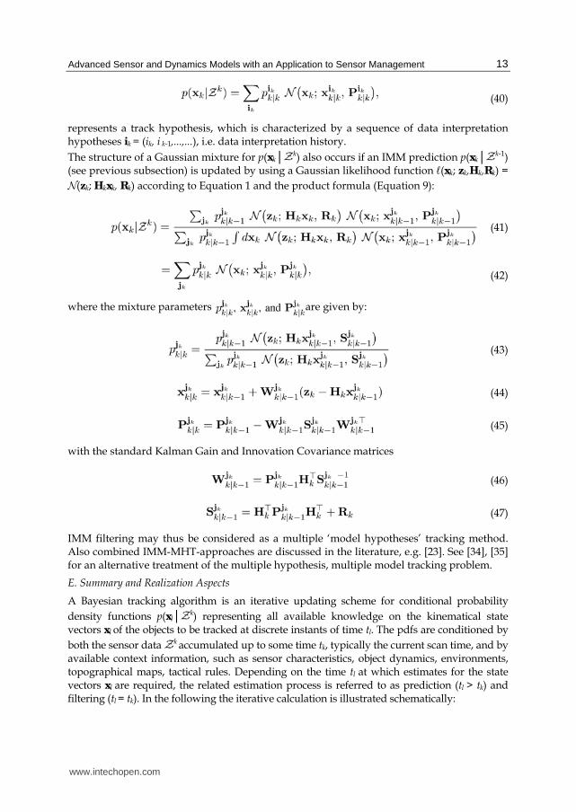
According to the Equation 1, this likelihood function implies that p(xk│ k) becomes a Gaussian mixture, a weighted sum of Gaussians, whose parameters are obtained by exploiting the product formula (9).

D. Gaussian Mixtures and Multiple Hypothesis Tracking

In many applications, such as group target tracking with possibly unresolved measurements [26], in ground moving target tracking with STAP radar [21], or target tracking with a phasedarray radar in the presence of jamming [10], the sensor model is described by a

likelihood function of the type ℓ(xk; Zk, nk) ∝ p(Zk, nk│ik, xk) p(ik│xk) [20]. Such

likelihood functions, which are essentially characterized by taking different data interpretation hypotheses ik into account, are the basis for Multiple Hypothesis Tracking algorithms (MHT, see [5]). In this context, each mixture component of the pdfs that result from Bayes’ Rule and a Gaussian mixture prediction,

www.intechopen.com


13

(40)

represents a track hypothesis, which is characterized by a sequence of data interpretation hypotheses ik = (ik, i k-1,...,...), i.e. data interpretation history.

The structure of a Gaussian mixture for p(xk│ k) also occurs if an IMM prediction p(xk│ k-1) (see previous subsection) is updated by using a Gaussian likelihood function ℓ(xk; zk,Hk,Rk) =

N(zk; Hkxk, Rk) according to Equation 1 and the product formula (Equation 9):

(41)

(42)

where the mixture parameters are given by:

(43)

(44)

(45)

with the standard Kalman Gain and Innovation Covariance matrices

(46)

(47)

IMM filtering may thus be considered as a multiple ‘model hypotheses’ tracking method. Also combined IMM-MHT-approaches are discussed in the literature, e.g. [23]. See [34], [35] for an alternative treatment of the multiple hypothesis, multiple model tracking problem.

E. Summary and Realization Aspects

A Bayesian tracking algorithm is an iterative updating scheme for conditional probability

density functions p(xl│ k) representing all available knowledge on the kinematical state vectors xl of the objects to be tracked at discrete instants of time tl. The pdfs are conditioned by

both the sensor data k accumulated up to some time tk, typically the current scan time, and by

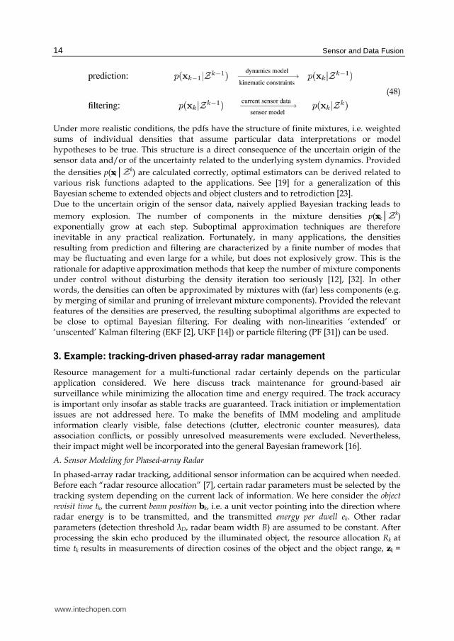
available context information, such as sensor characteristics, object dynamics, environments, topographical maps, tactical rules. Depending on the time tl at which estimates for the state vectors xl are required, the related estimation process is referred to as prediction (tl > tk) and filtering (tl = tk). In the following the iterative calculation is illustrated schematically:

www.intechopen.com


14

(48)

Under more realistic conditions, the pdfs have the structure of finite mixtures, i.e. weighted sums of individual densities that assume particular data interpretations or model hypotheses to be true. This structure is a direct consequence of the uncertain origin of the sensor data and/or of the uncertainty related to the underlying system dynamics. Provided

the densities p(xl│ k) are calculated correctly, optimal estimators can be derived related to various risk functions adapted to the applications. See [19] for a generalization of this Bayesian scheme to extended objects and object clusters and to retrodiction [23]. Due to the uncertain origin of the sensor data, naively applied Bayesian tracking leads to

memory explosion. The number of components in the mixture densities p(xk│ k) exponentially grow at each step. Suboptimal approximation techniques are therefore inevitable in any practical realization. Fortunately, in many applications, the densities resulting from prediction and filtering are characterized by a finite number of modes that may be fluctuating and even large for a while, but does not explosively grow. This is the rationale for adaptive approximation methods that keep the number of mixture components under control without disturbing the density iteration too seriously [12], [32]. In other words, the densities can often be approximated by mixtures with (far) less components (e.g. by merging of similar and pruning of irrelevant mixture components). Provided the relevant features of the densities are preserved, the resulting suboptimal algorithms are expected to be close to optimal Bayesian filtering. For dealing with non-linearities ‘extended’ or ‘unscented’ Kalman filtering (EKF [2], UKF [14]) or particle filtering (PF [31]) can be used.

3. Example: tracking-driven phased-array radar management

Resource management for a multi-functional radar certainly depends on the particular application considered. We here discuss track maintenance for ground-based air surveillance while minimizing the allocation time and energy required. The track accuracy is important only insofar as stable tracks are guaranteed. Track initiation or implementation issues are not addressed here. To make the benefits of IMM modeling and amplitude information clearly visible, false detections (clutter, electronic counter measures), data association conflicts, or possibly unresolved measurements were excluded. Nevertheless, their impact might well be incorporated into the general Bayesian framework [16].

A. Sensor Modeling for Phased-array Radar

In phased-array radar tracking, additional sensor information can be acquired when needed. Before each “radar resource allocation” [7], certain radar parameters must be selected by the tracking system depending on the current lack of information. We here consider the object revisit time tk, the current beam position bk, i.e. a unit vector pointing into the direction where radar energy is to be transmitted, and the transmitted energy per dwell ek. Other radar parameters (detection threshold ┣D, radar beam width B) are assumed to be constant. After processing the skin echo produced by the illuminated object, the resource allocation Rk at time tk results in measurements of direction cosines of the object and the object range, zk =

www.intechopen.com


15

( u k, v k, r k), along with the signal amplitude ak. A single dwell may be insufficient for

object detection and subsequent fine localization. Let denote the number of dwells

needed for a successful detection and the set of the corresponding beam

positions. Each radar allocation is thus characterized by the tuple Rk = (tk,Bk, , ek, zk, ak).

The sequence of successive allocations is denoted by Rk = {Rk,R k-1}.

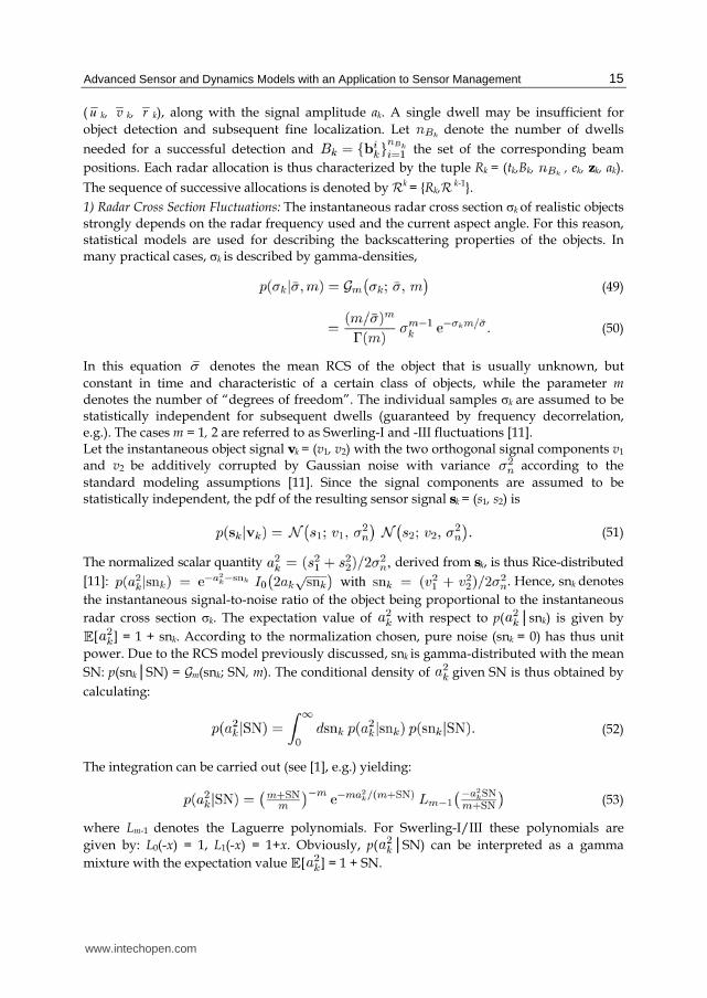
1) Radar Cross Section Fluctuations: The instantaneous radar cross section k of realistic objects strongly depends on the radar frequency used and the current aspect angle. For this reason, statistical models are used for describing the backscattering properties of the objects. In many practical cases, k is described by gamma-densities,

(49)

(50)

In this equation σ denotes the mean RCS of the object that is usually unknown, but

constant in time and characteristic of a certain class of objects, while the parameter m denotes the number of “degrees of freedom”. The individual samples k are assumed to be statistically independent for subsequent dwells (guaranteed by frequency decorrelation, e.g.). The cases m = 1, 2 are referred to as Swerling-I and -III fluctuations [11]. Let the instantaneous object signal vk = (v1, v2) with the two orthogonal signal components v1

and v2 be additively corrupted by Gaussian noise with variance according to the

standard modeling assumptions [11]. Since the signal components are assumed to be statistically independent, the pdf of the resulting sensor signal sk = (s1, s2) is

(51)

The normalized scalar quantity derived from sk, is thus Rice-distributed

[11]: . Hence, snk denotes

the instantaneous signal-to-noise ratio of the object being proportional to the instantaneous

radar cross section k. The expectation value of with respect to p( │snk) is given by

[ ] = 1 + snk. According to the normalization chosen, pure noise (snk = 0) has thus unit

power. Due to the RCS model previously discussed, snk is gamma-distributed with the mean

SN: p(snk│SN) = Gm(snk; SN, m). The conditional density of given SN is thus obtained by

calculating:

(52)

The integration can be carried out (see [1], e.g.) yielding:

(53)

where Lm-1 denotes the Laguerre polynomials. For Swerling-I/III these polynomials are

given by: L0(-x) = 1, L1(-x) = 1+x. Obviously, p( │SN) can be interpreted as a gamma

mixture with the expectation value [ ] = 1 + SN.

www.intechopen.com


16

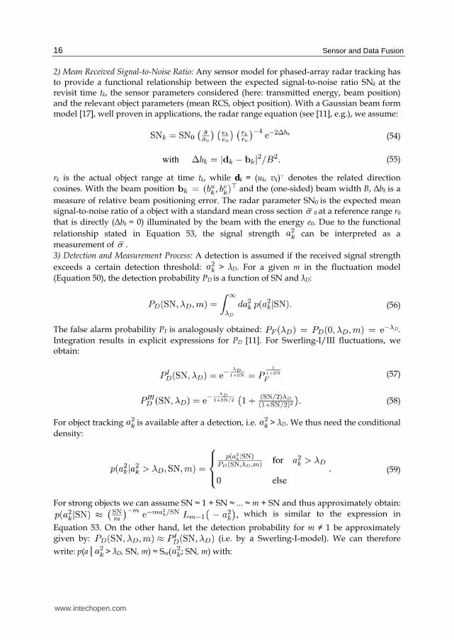
2) Mean Received Signal-to-Noise Ratio: Any sensor model for phased-array radar tracking has to provide a functional relationship between the expected signal-to-noise ratio SNk at the revisit time tk, the sensor parameters considered (here: transmitted energy, beam position) and the relevant object parameters (mean RCS, object position). With a Gaussian beam form model [17], well proven in applications, the radar range equation (see [11], e.g.), we assume:

(54)

(55)

rk is the actual object range at time tk, while dk = (uk, vk)e denotes the related direction

cosines. With the beam position and the (one-sided) beam width B, Δbk is a

measure of relative beam positioning error. The radar parameter SN0 is the expected mean signal-to-noise ratio of a object with a standard mean cross section σ 0 at a reference range r0

that is directly (Δbk = 0) illuminated by the beam with the energy e0. Due to the functional

relationship stated in Equation 53, the signal strength can be interpreted as a

measurement of σ .

3) Detection and Measurement Process: A detection is assumed if the received signal strength

exceeds a certain detection threshold: > ┣D. For a given m in the fluctuation model

(Equation 50), the detection probability PD is a function of SN and ┣D:

(56)

The false alarm probability PF is analogously obtained: .

Integration results in explicit expressions for PD [11]. For Swerling-I/III fluctuations, we obtain:

(57)

(58)

For object tracking is available after a detection, i.e. > ┣D. We thus need the conditional

density:

(59)

For strong objects we can assume SN ≈ 1 + SN ≈ ... ≈ m + SN and thus approximately obtain:

which is similar to the expression in

Equation 53. On the other hand, let the detection probability for m ≠ 1 be approximately

given by: (i.e. by a Swerling-I-model). We can therefore

write: p(a│ > ┣D, SN, m) ≈ Sm( ; SN, m) with:

www.intechopen.com


17

(60)

Let us furthermore assume that monopulse localization after detection result in bias-free measurements of the direction cosines and range with Gaussian measurement errors.

According to [11], the standard deviations depend on the beam width B and the

instantaneous snk in the following manner: Since snk is

unknown, in the last approximation is used as a bias-free estimate of snk ( [ ] = 1 + snk).

The range error is assumed to be Gaussian with a constant standard deviation r. Evidently, this model of the measurement process does not depend on the RCS fluctuation model.

B. Bayesian Tracking Algorithms Revisited

According to the previous discussion, object tracking is an iterative updating scheme for

conditional probability densities p(xk│Rk) that describe the current object state xk given all

available resource allocations Rk and the underlying a priori information in terms of

statistical models. The processing of each new measurement zk via Bayes’ Rule establishes a recursive relation between the densities at two consecutive revisit times (a prediction step followed by filtering).

(61)

with jk = (jk,..., jk-n+1) denoting a particular model history, i.e. a sequence of possible hypotheses

regarding the object dynamics model from a certain observation at time tk-n+1 up to the most

recent measurement at time tk (“n scans back”). In the case of a single dynamics model (r =

1), the prediction densities p(xk│Rk-1) are strictly given by Gaussians (standard Kalman

prediction). For n = 1, p(xk│Rk-1) is approximated by a mixture with r components according

to the r dynamics models used. GPB2 and standard IMM algorithms are possible

realizations of this scheme [3]. For standard IMM, the approximations are made after the

prediction, but before the filtering step, while for GPB2 they are applied after the filtering

step. Hence, GPB2 requires more computational effort. For details see [3].

2) Processing of Signal Strength Information: Let us treat the normalized mean RCS of the

object, sk = σ k/σ 0, as an additional component of the state vector. Since the signal strength

after a detection occurred may be viewed as a measurement of sk, let us consider the

augmented conditional density

(62)

The calculation of p(xk│Rk) was discussed in section 2. For the remaining density p(sk│xk,Rk),

an application of Bayes’ Rule yields up to a normalizing constant:

(63)

www.intechopen.com


18

Let us furthermore assume that p(sk│xk,Rk-1) are given by inverse gamma densities,

(64)

which are defined by:

(65)

where s is the expectation of this density, s = [s] > 0, ┤ a parameter ┤ > 1. For ┤ > 2, the

related variance exists: V[s] = s2/(┤ - 2). This class of densities is invariant under the

successive application of Bayes Rule according to Equation 63, since up to normalization we

obtain:

(66)

(67)

(68)

where the parameters α k, s k, and ┤k are given by:

(69)

(70)

(71)

With reference to sk the density (sk; s k, ┤k) is correctly normalized. Evidently, α k depends

on the object position (α k = α k(rk, uk, vk)). In order to preserve the factorization of p(xk, sk│Rk)

in a normal mixture related to the kinematic properties of the object xk and an inverse gamma density related to its RCS sk, we use the approximation:

(72)

where r k, u k, v k are the MMSE estimates for rk, uk and vk derived from p(xk│Rk). Hence, α k

compensates both the estimated positioning error of the radar beam and the propagation

loss due to the radar equation. Assuming sk to be constant, we have (sk; s k│k-1, ┤k│k)=

-1(sk; s k-1, ┤k│k-1). In principle, a dynamics model describing temporal changes of the

radar cross section might be introduced.

C. Adaptive Bayesian Sensor Management

The tracking results are essential for adaptive radar revisit time control, the selection of the

transmitted radar energy, and the design of intelligent algorithms for local search.

www.intechopen.com


19

1) Adaptive Radar Revisit Time Control: The time tk when a radar allocation Rk should take place is determined by the current lack of information conveniently described [17] by the

error covariance matrix Pk│k-1 of the predicted state estimate xk│k-1. Since p(xk│Rk-1) is a

normal mixture, xk│k-1 and Pk│k-1 are given by:

(73)

(74)

The covariance matrix

of the individual mixture components grow the faster in time

the more often maneuvers are assumed in the corresponding model histories. This has an impact on the total covariance matrix Pk│k-1 according to the corresponding weighting

factors . In addition, Pk│k-1 is “broadened” by the positively definite spread terms

( - xk│k-1) ( - xk│k-1)e. Obviously, the adaptive IMM modeling affects Pk│k-1 in a

rather complicated way. A scalar measure of the information deficit is provided, e.g., by the largest eigenvalue of the covariance matrix of the predicted object direction (in terms of u, v). Let it be denoted by Gk│k-1. A track update is allocated when the Gk│k-1 exceeds a predetermined proportion of the squared radar beam width B:

(75)

The relative track accuracy v0 introduced by this criterion is a measure of the minimum track quality required and a parameter to be optimized. In many practical applications, v0 = 0.3 is a reasonable choice [17]. 2) Transmitted Radar Energy Selection: In view of the tracking system, the sensor performance

is mainly characterized by the signal-to-noise ratio that determines both, the detection

probability and the measurement error. By suitably choosing the transmitted energy per

dwell ek, the expected signal-to-noise ratio SNk│k-1 can be kept constant during tracking.

Besides v0, SNk│k-1 is an additional parameter subject to optimization. Since v0 may be viewed

as a measure of the beam positioning error, the energy ek at time tk is defined by this

condition (Equation 54):

(76)

(77)

By this particular choice, the influence of the radar range equation is compensated (at least for a certain range interval). For the mean radar cross section σ either a worst-case

assumption or estimates from object amplitude information can be used. The track quality v0

also affects the transmitted energy. As a side effect of this choice, the standard deviations of the u, v-measurements are kept constant on an average.

www.intechopen.com


20

3) Bayesian Local Search Procedures: Intelligent algorithms for beam positioning and local search are crucial for IMM-type phased-array tracking. Overly simple strategies may easily destroy the benefits of the adaptive dynamics model, because track loss immediately after a model switch can easily occur. To avoid this phenomenon, we adapt the optimal approach

based on the predicted densities p(xk│Rk-1) proposed in [17] to IMM tracking [24].

1. The beam position of the first dwell at time tk is simply given by the predicted

direction dk│k-1 to be derived from the predicted density function p(xk│Rk-1).

2. If no detection occurs in the first dwell, this very result provides useful information on the target. We thus have to calculate the conditional density of the target state given the

event : ‘no detection at time tk in the direction ’.

3. An application of Bayes’ Rule directly yields:

(78)

up to a normalizing factor. In this expression, the detection probability PD depends on the expected SN (Equation 54) and thus on the current beam and target position bk, dk.

4. The two dimensional density can easily be calculated on a grid. The

beam position for the next dwell is then simply provided by its maximum. 5. This computational scheme for Bayesian local search is repeated until a detection

occurs. Since the maximum of the densities is searched, the

computation of the normalization integral is not required. Numerically efficient realizations are possible.

Alternatively, might be used for calculating the expected SN in a certain

direction bk:

Searching the maximum of SN(bk) results in a different local search strategy. In the examples

considered below, however, no significant performance improvements were observed.

Nevertheless, there might be applications where the maximization of SN(bk) is

advantageous (e.g. for track recovery in case of intermittent operating modes).

This local search scheme exploits ‘negative’ evidence, as also here the lack of an expected

measurement carries information on the current target position. We here in particular

observe a direct impact on adaptive sensor management. Again, the prerequisite for dealing

with negative evidence is an adequate sensor performance model. As in the case of

resolution phenomena (section 2), the processing of negative sensor evidence implies

mixture densities with possibly negative mixture coefficients, i.e. not each mixture

component has a direct probabilistic interpretation. As the mixture coefficients sum up to

one, the overall density nevertheless has a well-defined probabilistic meaning.

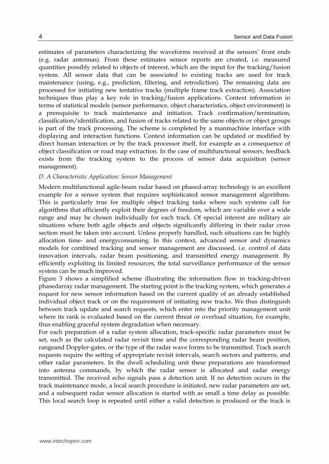
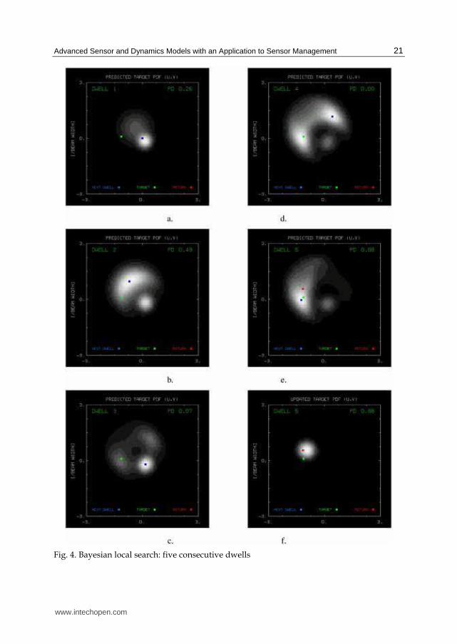
Figure 4 illustrates this scheme of Bayesian local search for a particular example. In Figure

4a the predicted pdf , a mixture density, is shown for some time tk. The target is

expected to be in the bright region with high probability , the true target position being

indicated by a green dot. The blue dot denotes the beam position of the next dwell. The

related detection probability is 26%. However, no detection occurred during the first dwell

www.intechopen.com


21

Fig. 4. Bayesian local search: five consecutive dwells

www.intechopen.com


22

1. We thus calculate the conditional pdf given that event. As visible in

Figure 4b, it differs significantly from . The previous maximum decreased in

height, while the global maximum is at a different location. Again no detection occurred; the

resulting density reflecting the two pieces of ‘negative’ evidence

is shown in Figure 4c. Now the search algorithm decides to look again near

the position at dwell 1. Although wrong in this case, this does not seem to be unreasonable. In addition, two smaller local maxima appear that increase in size as in the next dwell also no detection occurred. According to Figure 4d the next decision is ambiguous. We finally obtain a decision which leads to success. The last picture shows the updated pdf (Figure 4f).

4. Discussion of numerical simulation results

Simulation results provide hints as to what extent the total performance of multiple-object air surveillance by phased-array can be improved by using adaptive techniques for combined tracking and sensor control. The following four questions are addressed: 1. What resource savings (allocation time, energy) can be expected by using adaptive

dynamics models? 2. How should the IMM dynamics modeling be designed (e.g. number of models,

transition matrix)? 3. What energy savings can be expected by exploiting object amplitude information for

sensor control? 4. Why is Bayesian local search important when adaptive dynamics models are used for

revisit time control?

A. Discussion of Simulation Scenarios

In general we follow the parameter and threshold settings recommended in [17]. To exclude

false alarms due to receiver noise, the false alarm probability is PF = 10-4. False returns due to clutter or ECM are not considered. The standard deviation of the measurement errors in object range is r = 100 m, while the the radar beam width is B = 1°. We assume a minimum time interval of 20 ms between consecutive dwells on a particular object and statistically independent signal amplitudes (frequency decorrelation, e.g.). The reference range is set to r0 = 80 km. 1) IMM Modeling Parameters: Antenna coordinates (direction cosines, range) are used also for tracking; non-linearities introduced by these non-Cartesian coordinates are taken into account [16]. In each component uk, vk, rk the state vector is given by position, speed, and acceleration. For the sake of simplicity, we consider a block diagonal system matrix defined by

(79)

(80)

with Δtk = tk – tk-1. The maneuvering capability of the objects is thus characterized by two parameters: maneuver correlation time θ and acceleration width Σ. For r = 2, 3 we consider the parameter sets:

www.intechopen.com


23

• M1 (worst-case model): Σ1 = 60 m/s2, θ1 = 30 s

• M2 (best-case model): Σ2 = 1 m/s2, θ2 = 10 s

• M3 (medium-case model): Σ3 = 30 m/s2, θ3 = 30 s The matrices of the model transition probabilities are given by:

(81)

We observed that the performance does not critically depend on the particular switching

probabilities pij chosen. A detailed mismatch analysis, however, has not been performed. A

track is considered to be lost if more than 50 dwells occur in the local search of if the beam

positioning error Δbk is greater than 3B. We thus permit even a rather extensive local search

that correspondingly burdens the total energy budget. In all simulations considered below

(1000 runs) the relative frequency of track loss is less than 2%.

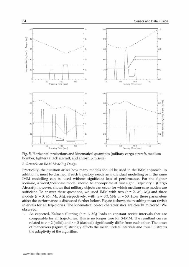
2) Selected Benchmark Trajectories: The horizontal projection of four standard benchmark

trajectories (military cargo aircraft, medium bomber, fighter/attack aircraft, and anti-ship

missile) is shown in Figure 5 along with representative kinematical characteristics such as

acceleration (solid line), range (dashed), height (dotted), and speed (solid). They have been

proposed in [8], [9] and cover a rather wide range of militarily relevant objects. The missile

trajectory might serve to explore the performance limits of the algorithms. In principle,

missiles can execute even stronger maneuvers. It is questionable, however, if for those

objects and their individual missions the dynamics models discussed above remain

applicable. All objects are tracked over a period of 180 s. The RCS fluctuations are described

by a Swerling-III model. The mean cross sections significantly vary from object to object (4.,

2., 1.2, .5 m2).

3) Measures of Performance Considered: The discussion is confined to a few intuitively clear

and simple performance measures obtained by Monte-Carlo simulation (1000 runs). In

general a single performance measure is not sufficient as there may exist applications where

the transmitted energy is the limiting factor, while in a different scenario the number of

radar allocations must be kept low.

The adaptivity becomes visible if the performance is evaluated as a function of the tracking

time that can be compared with the kinematics of the individual trajectories (Figure 5). Here

we used histograms with 100 cells. In particular we considered: the mean revisit intervals,

the mean number of dwells for a successful update, the mean number of sensor allocations

in total required for track maintenance, the mean energy spent for a successful allocation,

the mean energy totally spent for track maintenance, and the mean RCS of the objects

estimated during tracking.

Four tracking filters were compared: worst-case Kalman filter (KF), standard IMM filter

with two or three models, respectively (S-IMM2,3), and IMM-MHT filtering with model

histories of length n = 4. For IMM-MHT with n > 4, the performance characteristics change

only slightly. We thus conclude that n = 4 already provides a good approximation to

optimal filtering (at least for the scenarios considered here). With reference to object

amplitude information we considered three cases: 1) the object RCS σ is known and used

for energy management. 2) The mean RCS σ is unknown and to be estimated during

tracking. 3) A worst-case assumption is used for all objects (σ = 0.5 m2).

www.intechopen.com


24

Fig. 5. Horizontal projections and kinematical quantities (military cargo aircraft, medium bomber, fighter/attack aircraft, and anti-ship missile)

B. Remarks on IMM Modeling Design

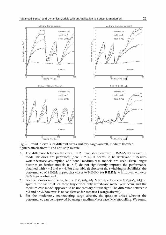
Practically, the question arises how many models should be used in the IMM approach. In addition it must be clarified if each trajectory needs an individual modelling or if the same IMM modelling can be used without significant loss of performance. For the fighter scenario, a worst/best-case model should be appropriate at first sight. Trajectory 1 (Cargo Aircraft), however, shows that military objects can occur for which medium-case models are sufficient. To answer these questions, we used IMM with two (r = 2, M1, M2) and three models (r = 3, M1, M2, M3), respectively, with v0 = 0.3, SNk│k-1 = 50. How these parameters affect the performance is discussed further below. Figure 6 shows the resulting mean revisit intervals for all trajectories. The kinematical object characteristics are clearly mirrored. We observed: 1. As expected, Kalman filtering (r = 1, M1) leads to constant revisit intervals that are

comparable for all trajectories. This is no longer true for S-IMM. The resultant curves related to r = 2 (solid) and r = 3 (dashed) significantly differ from each other. The onset of maneuvers (Figure 5) strongly affects the mean update intervals and thus illustrates the adaptivity of the algorithm.

www.intechopen.com


25

Fig. 6. Revisit intervals for different filters: military cargo aircraft, medium bomber, fighter/attack aircraft, and anti-ship missile

2. The difference between the cases r = 2, 3 vanishes however, if IMM-MHT is used. If model histories are permitted (here n = 4), it seems to be irrelevant if besides worst/bestcase assumption additional medium-case models are used. Even longer histories or further models (r > 3) do not significantly improve the performance obtained with r = 2 and n = 4. For a suitable (!) choice of the switching probabilities, the performance of S-IMM4 approaches closes to B-IMM2; for B-IMM4 no improvement over B-IMM2 was observed.

3. For the bomber and the fighter, S-IMM3 (M1, M2, M3) outperforms S-IMM2 (M1, M2), in spite of the fact that for these trajectories only worst-case maneuvers occur and the medium-case model appeared to be unnecessary at first sight. The difference between r = 2 and r = 3, however, is not as clear as for scenario 1 (cargo aircraft).

4. For the moderately maneuvering cargo aircraft, the question arises whether the performance can be improved by using a medium/best-case IMM modelling. We found

www.intechopen.com


26

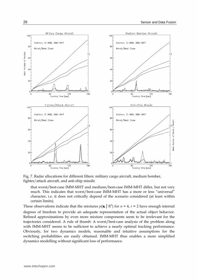
Fig. 7. Radar allocations for different filters: military cargo aircraft, medium bomber, fighter/attack aircraft, and anti-ship missile

that worst/best-case IMM-MHT and medium/best-case IMM-MHT differ, but not very much. This indicates that worst/best-case IMM-MHT has a more or less “universal” character, i.e. it does not critically depend of the scenario considered (at least within certain limits).

These observations indicate that the mixtures p(xk│Rk) for n = 4, r = 2 have enough internal

degrees of freedom to provide an adequate representation of the actual object behavior.

Refined approximations by even more mixture components seem to be irrelevant for the

trajectories considered. A rule of thumb: A worst/best-case analysis of the problem along

with IMM-MHT seems to be sufficient to achieve a nearly optimal tracking performance.

Obviously, for two dynamics models, reasonable and intuitive assumptions for the

switching probabilities are easily obtained. IMM-MHT thus enables a more simplified

dynamics modelling without significant loss of performance.

www.intechopen.com


27

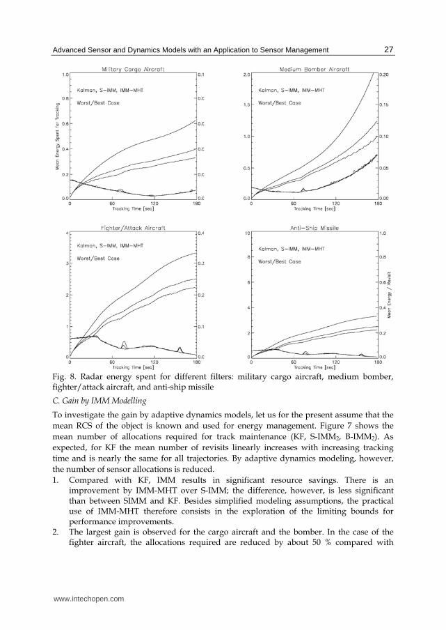
Fig. 8. Radar energy spent for different filters: military cargo aircraft, medium bomber, fighter/attack aircraft, and anti-ship missile

C. Gain by IMM Modelling

To investigate the gain by adaptive dynamics models, let us for the present assume that the

mean RCS of the object is known and used for energy management. Figure 7 shows the

mean number of allocations required for track maintenance (KF, S-IMM2, B-IMM2). As

expected, for KF the mean number of revisits linearly increases with increasing tracking

time and is nearly the same for all trajectories. By adaptive dynamics modeling, however,

the number of sensor allocations is reduced.

1. Compared with KF, IMM results in significant resource savings. There is an improvement by IMM-MHT over S-IMM; the difference, however, is less significant than between SIMM and KF. Besides simplified modeling assumptions, the practical use of IMM-MHT therefore consists in the exploration of the limiting bounds for performance improvements.

2. The largest gain is observed for the cargo aircraft and the bomber. In the case of the fighter aircraft, the allocations required are reduced by about 50 % compared with

www.intechopen.com


28

worstcase Kalman filtering. Even during the 7 g weaving of the missile, some advantages of the IMM modeling can be observed.

Figure 7 shows the mean number of dwells per revisit. Up to peaks corresponding with the onset of maneuvers, it is constant and roughly equal for all filters and trajectories. The more adaptive the filter is, the higher the peaks are, i.e. the larger the revisit intervals can be during inertial flight. The peaks thus indicate that for abrupt maneuvers a local search might be required. This is the price to be paid for increased adaptivity. Evidently, intelligent algorithms for beam positioning and local search are essential for IMM phased-array tracking. These observations are consistent with Figure 8, which shows the mean energy spent for track maintenance (relative units). Besides the object maneuvers, these curves are influenced by the current object range (Figure 5, dotted line). In addition, the mean energy spent per revisit is displayed. Up to characteristic peaks, the energy per revisit is roughly the same for all tracking filters.

D. On the Quality of RCS Estimates

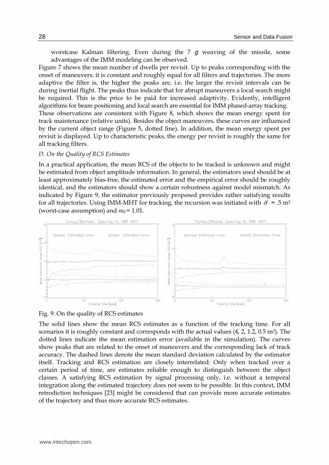
In a practical application, the mean RCS of the objects to be tracked is unknown and might be estimated from object amplitude information. In general, the estimators used should be at least approximately bias-free, the estimated error and the empirical error should be roughly identical, and the estimators should show a certain robustness against model mismatch. As indicated by Figure 9, the estimator previously proposed provides rather satisfying results for all trajectories. Using IMM-MHT for tracking, the recursion was initiated with σ = .5 m2

(worst-case assumption) and m0 = 1.01.

Fig. 9. On the quality of RCS estimates

The solid lines show the mean RCS estimates as a function of the tracking time. For all scenarios it is roughly constant and corresponds with the actual values (4, 2, 1.2, 0.5 m2). The dotted lines indicate the mean estimation error (available in the simulation). The curves show peaks that are related to the onset of maneuvers and the corresponding lack of track accuracy. The dashed lines denote the mean standard deviation calculated by the estimator itself. Tracking and RCS estimation are closely interrelated: Only when tracked over a certain period of time, are estimates reliable enough to distinguish between the object classes. A satisfying RCS estimation by signal processing only, i.e. without a temporal integration along the estimated trajectory does not seem to be possible. In this context, IMM retrodiction techniques [23] might be considered that can provide more accurate estimates of the trajectory and thus more accurate RCS estimates.

www.intechopen.com


29

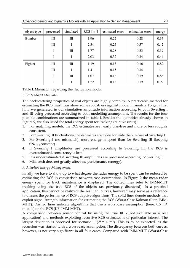
Table I. Mismatch regarding the fluctuation model

E. RCS Model Mismatch

The backscattering properties of real objects are highly complex. A practicable method for estimating the RCS must thus show some robustness against model mismatch. To get a first hint, we generated in our simulation amplitude information according to both Swerling I and III being processed according to both modelling assumptions. The results for the four possible combinations are summarized in table I. Besides the quantities already shown in Figure 9, we also listed the total energy spent for tracking (relative units). 1. For matching models, the RCS estimates are nearly bias-free and more or less roughly

consistent. 2. For Swerling III fluctuations, the estimates are more accurate than in case of Swerling I. 3. For Swerling I (no mismatch), more energy is spent than for Swerling III (keeping

SNk│k-1 constant). 4. If Swerling I amplitudes are processed according to Swerling III, the RCS is

overestimated, consistency is lost. 5. It is underestimated if Swerling III amplitudes are processed according to Swerling I. 6. Mismatch does not greatly affect the performance (energy).

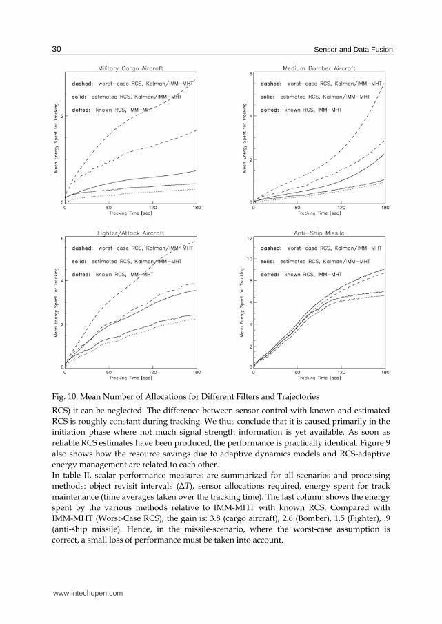
F. Adaptive Energy Management.

Finally we have to show up to what degree the radar energy to be spent can be reduced by estimating the RCS in comparison to worst-case assumptions. In Figure 9 the mean radar energy spent for track maintenance is displayed. The dotted lines refer to IMM-MHT tracking using the true RCS of the objects (as previously discussed). In a practical application, this cannot be realized; the resultant curves, however, may serve as a reference to discuss the performance of RCS-adaptive algorithms. The solid lines denote methods that exploit signal strength information for estimating the RCS (Worst-Case Kalman filter, IMM-MHT). Dashed lines indicate algorithms that use a worst-case assumption (here: 0.5 m2, missile) on the RCS (KF, IMM-MHT). A comparison between sensor control by using the true RCS (not available in a real application) and methods exploiting recursive RCS estimates is of particular interest. The largest deviation is observed for scenario 1 (σ = 4 m2). This is to be expected, as the

recursion was started with a worst-case assumption. The discrepancy between both curves, however, is not very significant in all four cases. Compared with IMM-MHT (Worst-Case

www.intechopen.com


30

Fig. 10. Mean Number of Allocations for Different Filters and Trajectories

RCS) it can be neglected. The difference between sensor control with known and estimated

RCS is roughly constant during tracking. We thus conclude that it is caused primarily in the

initiation phase where not much signal strength information is yet available. As soon as

reliable RCS estimates have been produced, the performance is practically identical. Figure 9

also shows how the resource savings due to adaptive dynamics models and RCS-adaptive

energy management are related to each other.

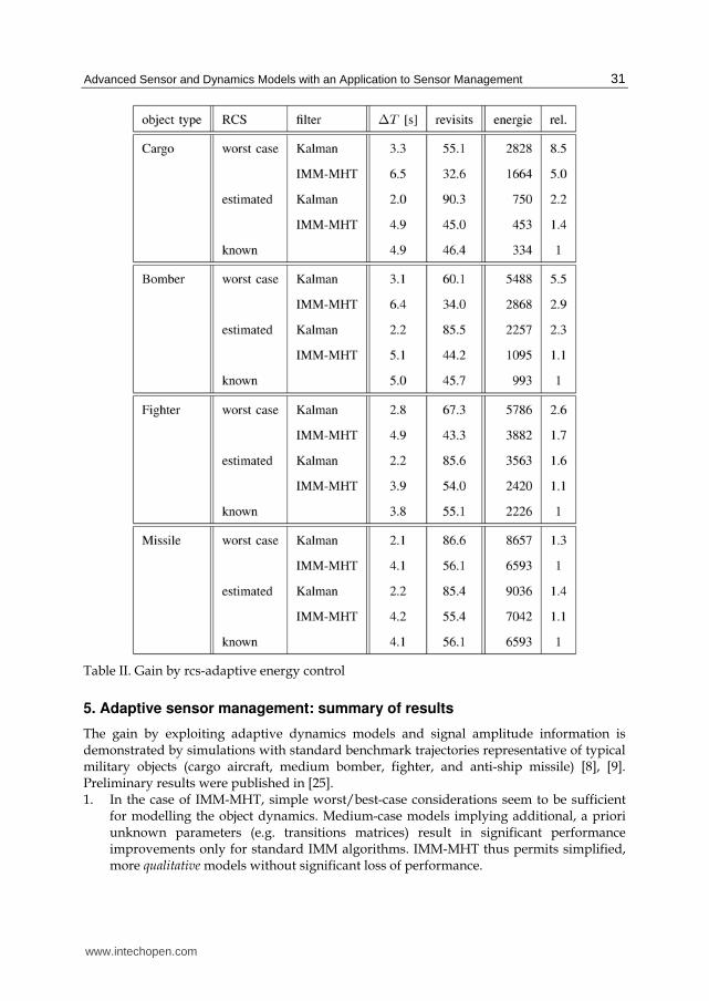
In table II, scalar performance measures are summarized for all scenarios and processing

methods: object revisit intervals (ΔT), sensor allocations required, energy spent for track

maintenance (time averages taken over the tracking time). The last column shows the energy

spent by the various methods relative to IMM-MHT with known RCS. Compared with

IMM-MHT (Worst-Case RCS), the gain is: 3.8 (cargo aircraft), 2.6 (Bomber), 1.5 (Fighter), .9

(anti-ship missile). Hence, in the missile-scenario, where the worst-case assumption is

correct, a small loss of performance must be taken into account.

www.intechopen.com


31

Table II. Gain by rcs-adaptive energy control

5. Adaptive sensor management: summary of results

The gain by exploiting adaptive dynamics models and signal amplitude information is demonstrated by simulations with standard benchmark trajectories representative of typical military objects (cargo aircraft, medium bomber, fighter, and anti-ship missile) [8], [9]. Preliminary results were published in [25]. 1. In the case of IMM-MHT, simple worst/best-case considerations seem to be sufficient

for modelling the object dynamics. Medium-case models implying additional, a priori unknown parameters (e.g. transitions matrices) result in significant performance improvements only for standard IMM algorithms. IMM-MHT thus permits simplified, more qualitative models without significant loss of performance.

www.intechopen.com


32

2. Compared with worst-case Kalman filtering, IMM results in considerable resource savings. The reduction with respect to the number of allocations required and the energy spent for track maintenance is roughly comparable and varies between 50 and 100% depending on the scenario considered. Essentially, the savings are due to longer revisit intervals on an average.

3. IMM-MHT improves on standard IMM algorithms. The difference, however, is less significant than between standard IMM and worst-case Kalman filtering. Besides simplified modelling assumptions, the practical use of IMM-MHT primarily consists in the exploration of the theoretical boundaries that limit the performance improvements achievable by adaptive dynamics models.

4. Due to abrupt maneuvers after a longer inertial flight, IMM-type tracking must necessarily be complemented by efficient Bayesian algorithms for adaptive beam positioning and local search. If used, however, racking process remains highly stable, because all information on the possible dynamical behavior of the objects is taken into account.

5. By processing object amplitude information along the estimated trajectory, the a priori unknown RCS of the objects can (roughly) be estimated. The estimate is approximately bias-free; its variance corresponds with the empirical variance. It is closely related to the tracking process and might provide a contribution to object classification. Within certain limits, the method seems to be rather robust against model mismatch.

6. Compared with worst-case assumptions on the object RCS, significant energy savings can be obtained by exploiting amplitude information. Depending on the scenario considered, the gain is larger than the improvement achievable by adaptive dynamics models. The difference to algorithms that use of the correct object RCS (available in a simulation) is comparatively small and arises mainly in the initiation phase.

6. References

[1] M. Abramowitz and I.A. Segun. Handbook of Mathematical Functions, Dover (1965). [2] Y. Bar-Shalom, X.-R. Li, and T. Kirubarajan. Estimation with Applications to Tracking and

Navigation. Wiley & Sons, 2001. [3] Y. Bar-Shalom and X.-R. Li. Estimation and Tracking: Principles, Techniques, Software,

Boston, MA: Artech House, 1993. [4] J. Biermann. Understanding Military Information Processing - An Approach to Support

Intelligence in Defence and Security. In NATO Advanced Research Workshop on Data Fusion Technologies in Harbour Protection, Tallinn, Estonia, 2005.

[5] S. Blackman. Multiple Hypothesis Methods. In IEEE AES Magazine, 19, 1, p. 41–52, 2004. [6] S. Blackman and R. Populi. Design and Analysis of Modern Tracking Systems. Artech House,

1999. [7] R. J. Dempster, S. Blackman, S. H. Roszkowski, and D. M. Sasaki. IMM/MHT Solution to

Radar and Multisensor Benchmark Tracking Problems. In SPIE 3373, Signal and Data Processing of Small objects (1998).

[8] W. D. Blair, G.A. Watson, T. Kirubarajan, and Y. Bar-Shalom. Benchmark for Radar Resource Allocation and Tracking objects in the Presence of ECM. In IEEE TAES 35, No. 4 (1998).

[9] W. D. Blair, G. A. Watson, and K. W. Kolb. Benchmark Problem for Beam Pointing Control of Phased-Array Radar in the Presence of False Alarms and ECM. In Proceedings 1995 American Control Conference, Seattle WA (1994).

www.intechopen.com


33

[10] W. Blanding, W. Koch, and U. Nickel. Tracking Through Jamming Using ‘Negative’ Information. In Proc. of the 9th International Conference on Information Fusion FUSION 2006, Florence, Italy, July 2006. To appear also in IEEE TAES.

[11] Philip L. Bogler. Radar Principles with Applications to Tracking Systems. John Wiley & Sons (1990).

[12] W. Fleskes and G. van Keuk. On Single Target Tracking in Dense Clutter Environment - Quantitative Results. In Proc. of IEE International Radar Conference RADAR 1987, pp. 130-134.

[13] I. S. Gradshteyn and I. M. Ryzhik. Table of Integrals, Series, and Products, Academic Press (1979).

[14] D. L. Hall and J. Llinas (Eds.). Handbook of Multisensor Data Fusion. CRC Press, 2001. [15] Young-Hun Jung and Sun-Mog Hong. Modelling and Parameter Optimization of Agile

Beam Radar Tracking. In IEEE TAES, vol. 39, no. 1, p.13-33, Jan. 2003. [16] G. van Keuk. Multihypothesis Tracking with Electronically Scanned Radar”. In IEEE

AES 31, No. 3 (1995). [17] G. van Keuk and S. Blackman. On Phased-Array Tracking and Parameter Control. In

IEEE AES 29, No. 1 (1993). [18] T. Kirubarajan, Y. Bar-Shalom, W. D. Blair, and G. A. Watson. IMMPDAF Solution to

Benchmark for Radar Resource Allocation and Tracking Targets in the Presence of ECM”, IEEE AES 35, No. 4 (1998).

[19] W. Koch. A Bayesian Approach to Extended Object and Cluster Tracking using Random Matrices. In IEEE TAES, July 2008.

[20] W. Koch. On Exploiting ’Negative’ Sensor Evidence for object Tracking and Sensor Data Fusion. in Information Fusion, 8(1), 28-39, 2007.

[21] W. Koch. Ground Target Tracking with STAP Radar: Selected Tracking Aspects. Chapter 15 in: R. Klemm (Ed.), The Applications of Space-Time Adaptive Processing, IEE Publishers, 2004.

[22] W. Koch. Target Tracking. Chapter 8 in S. Stergiopoulos (Ed.), Signal Processing Handbook. CRC Press, 2001.

[23] W. Koch. Fixed-Interval Retrodiction Approach to Bayesian IMM-MHT for Maneuvering Multiple Targets. In IEEE TAES, 36, No. 1, (2000).

[24] W. Koch. On Adaptive Parameter Control for Phased-Array Tracking. Signal and Data Processing of Small Targets, SPIE Vol. 3809, pp. 444-455, Denver, USA, July 1999.

[25] W. Koch and G. van Keuk. On Bayesian IMM-Tracking for Phased-Array Radar. In Proc. DGON/ITG International Radar Symposium, IRS ’98, Conference Proceedings, p. 715-723, Mnchen (1998).

[26] W. Koch and G. van Keuk. Multiple Hypothesis Track Maintenance with Possibly Unresolved Measurements. IEEE TAES, 33, No. 3 (1997).

[27] W. Koch, J. Koller, and M. Ulmke. Ground object Tracking and Road Map Extraction. In ISPRS Journal on Photogrammetry & Remote Sensing, 61, 197-208, 2006.

[28] B. F. La Scala and B. Moran. Optimal Target Tracking with Restless Bandits. In Digital Signal Processing, vol. 16, no. 5, p. 479-87, Sept. 2006.

[29] B. F. La Scala, M. Rezaeian, and B. Moran. Optimal Adaptive Waveform Selection for Target Tracking. In Proc. of the 9th International Conference on Information Fusion, FUSION 2006, Florence, Italy, July 2006.

www.intechopen.com


34

[30] R. P. S. Mahler. ”Statistics 101” for Multisensor, Multitarget Data Fusion. In IEEE AES Magazine, 19, 1, p. 53–64, 2004.

[31] B. Ristic and N. Gordon. Beyond Kalman Filtering. Wiley, 2004. [32] D. Salmond. Mixture Reduction Algorithms for Target Tracking in Clutter. In SPIE, vol.

1305, April 1990, pp. 434-445. [33] P. W. Sarunic and R. J. Evans. Adaptive Update Rate Tracking using IMM Nearest

Neighbour Algorithm Incorporating Rapid Re-Looks. In IEE Proc.-Radar, Sonar, Navig., 144, No. 4 (1997)

[34] R. Streit and T. E. Luginbuhl. Probabilistic Multi-Hypothesis Tracking. Naval UnderseaWarfare Center Dahlgren Division, Research Report NUWC-NPT/10/428.

[35] M. Wieneke and W. Koch. The PMHT: Solutions to Some of its Problems. In Proc. of SPIE Signal and Data Processing of Small Targets, San Diego, USA, August 2007. Also submitted to ISIF Journal of Advances in Information Fusion.

www.intechopen.com

Sensor and Data FusionEdited by Nada Milisavljevic

ISBN 978-3-902613-52-3Hard cover, 436 pagesPublisher I-Tech Education and PublishingPublished online 01, February, 2009Published in print edition February, 2009

InTech EuropeUniversity Campus STeP Ri Slavka Krautzeka 83/A 51000 Rijeka, Croatia Phone: +385 (51) 770 447 Fax: +385 (51) 686 166www.intechopen.com

InTech ChinaUnit 405, Office Block, Hotel Equatorial Shanghai No.65, Yan An Road (West), Shanghai, 200040, China

Phone: +86-21-62489820 Fax: +86-21-62489821

Data fusion is a research area that is growing rapidly due to the fact that it provides means for combiningpieces of information coming from different sources/sensors, resulting in ameliorated overall systemperformance (improved decision making, increased detection capabilities, diminished number of false alarms,improved reliability in various situations at hand) with respect to separate sensors/sources. Different datafusion methods have been developed in order to optimize the overall system output in a variety of applicationsfor which data fusion might be useful: security (humanitarian, military), medical diagnosis, environmentalmonitoring, remote sensing, robotics, etc.

How to referenceIn order to correctly reference this scholarly work, feel free to copy and paste the following:

Wolfgang Koch (2009). Advanced Sensor and Dynamics Models with an Application to Sensor Management,Sensor and Data Fusion, Nada Milisavljevic (Ed.), ISBN: 978-3-902613-52-3, InTech, Available from:http://www.intechopen.com/books/sensor_and_data_fusion/advanced_sensor_and_dynamics_models_with_an_application_to_sensor_management

© 2009 The Author(s). Licensee IntechOpen. This chapter is distributedunder the terms of the Creative Commons Attribution-NonCommercial-ShareAlike-3.0 License, which permits use, distribution and reproduction fornon-commercial purposes, provided the original is properly cited andderivative works building on this content are distributed under the samelicense.

https://creativecommons.org/licenses/by-nc-sa/3.0/

Documents

Advanced Sensor and Dynamics Models with an Application to