Embed Size (px)
Citation preview

ILASS Americas, 25th Annual Conference on Liquid Atomization and Spray Systems, Pittsburgh, PA, May 2013
Advances and Challenges in Droplet and Spray Combustion
II. Toward a Unified Theory of Spray and Droplet Aerothermochemistry
H. H. Chiu* and J. S. Huang
**
*Institute of Aeronautics and Astronautics
National Cheng Kung University
Tainan, 701 Taiwan *The University of Illinois at Chicago, USA
**
Department of Mechanical Engineering
Taipei Chengshihi University
Taipei, 112 Taiwan
Abstract
The paper addresses four topics. First theme is the review of the progress and the new developments in spray
combustion focused on the universal spray combustion characteristics. Secondly, we present a theory of low
frequency oscillation induced by the shedding of fuel mass, momentum, vortex and thermal energy from combusting
sprays. The intrinsic sources of this oscillation are characterized by 24 physico-chemical parameters. We present a
series of theorems, describing the mechanisms of the oscillation and identified a family of Strouhal numbers and
their spectra. It is remarkable to conclude with a striking fact that all spray engines are prone to low frequency
oscillation because there are literally infinitely large families of the continuous bands of Strouhal spectra. High
frequency oscillation, in kilo-Hz range, is provoked by acoustic-chemistry inter-coupling and meets the Rayleigh
criterion. We identified 5 major sources of acoustic oscillation. Numerical examples of a series of Strouhal number,
their spectra of low and high frequency and intensity of oscillation are presented. Third topic concerns with the
engine performance optimization for fuel efficiency, minimum pollutant emission. We predicted the conditions of
achieving optimum performance in terms of the group combustion number. Numerical examples of optimization of
various types of spray engines are presented. Fourth subject is the development of the theory of flow separation and
reattachment. We analytically predicted the locations of separation and reattachment and a complete flow structure
in reversed flow regions in various engine components. Numerical sensitivity analysis is presented. These topics
have been the most prized unsolved problems in boundary layer theory, which Goldstein, Stewartson and many
scientists were unable to obtain an exact solution, except approximate solutions since 1930 till present time. The
paper concludes with the areas of future research.
Keywords: Spray combustion, Generalized Strouhal theory, Two-phase chemically reacting flow, Canonical
integration, Bi-characteristic integration.
**
Corresponding author: [email protected]
1. Introduction
The objectives of this paper are to present four fun-
damental themes: the modern canonical theory of spray
combustion, review of spray combustion 1930 to 2013
and two-phase chemically reacting as well as non-
reacting boundary layer fluid mechanics. We focus on
the following topics:
(1) Canonical theory focused on a modern spray
combustion analysis: covering four major types of
gasification mechanisms and two types of
combustion processes, flow field structure as well
as dynamic behavior associated with many natural
frequency behavior that make spray to be
inherently unstable because of the presence of
many spectra of Strouhal number. The theory
covers detailed flow structure, rates of the
interfacial exchange of mass momentum and
energy, and introduction of generalized Strouhal
theory in terms of flow elemental processes in the
immediate upstream, the recirculation zone and the
potential flow region infected by viscous effects
and shape change.
(2) Comprehensive review of spray combustion of
liquid fuel in subcritical and critical state, covering
structure dynamics of combustion and flow,
through a review of major experimental and
analytical works reported to this date to assess the
progress and challenge in droplet and spray
combustion. Optimization of engine performance is
also described.
(3) Modern theory of global boundary layer fluid flow,
addressing on the flow field structure, including,
velocity profiles in the upstream of separation point,
recirculation zone and after recirculation zone,
where the traditional boundary layer theory failed
to predict the flow except by approximate methods.
Theory also provides principle of similitude of
vortices, identification of the family of Strouhal
numbers and theory of spectra for the shedding of
major dynamic and thermo chemical properties,
drag coefficient and the geometrical properties,
including the location of separation and
reattachment points, length and width of
recirculation presented in universal formulas as
function of major parameters,. Flow field structure
of recalculating flow region, which has been one of
the prized unsolved problems that Goldstein and
Stewartson and various scientist in Cambridge and
other nations had actively researched. Impressive
progress has being made for practical application
over the past few centuries. However, majority of
the works are approximate solution and
experimental studies, and did not touch-in the heart
of the problems. Canonical theory is able to
provide an exact axiomatic representation of
Navier-Storkes equation for providing the first-
hand knowledge of the intrinsic behavior of these
flow fields in great depth.
(4) Combustion oscillation in two-phase chemically
reacting flow, which includes flow instability and
oscillation are clarified. In particular, we identified
the dynamic and energetic sources of the low
frequency oscillation due to the various shedding
processes and the acoustic-chemically coupled high
frequency oscillation. These studies reveals striking
facts that the liquid spray combustion has a large
family of Strouhal number continuous spectra,
which make the spray to be inherently highly
unstable thereby makes all the spray engines to
become highly susceptible to non-steady
disturbances in practical application. With all these
various oscillation, due to shedding of various flow
properties will lead to the formation of group wave
of high amplitude and enhanced rate of non-steady
exchange of the energy and momentum with
resonant mechanism, turbulent eddies and flow
expansion due to exothermicity, all of which
enhance the strength of turbulent flow and non-
steady flame oscillation.
(5) An attempt has been made to formulate a method of
the optimization of the combustion efficiency to
enhance the fuel saving and the minimization of
combustion related pollutants in liquid spray
engines which has been traditionally carried out by
trial and error, that is time consuming with high
cost penalty. Present study, based on analytical
formulation aided by numerical analysis, will be
able to determine the optimum conditions for
enhancing fuel efficiency of various spray engines
including, gas-turbine engines, liquid rockets,
hybrid rockets and Diesel engines and provide
practically useful means of designing optimum
atomizer. We also present the partition principle to
quantify the extent of contribution of each
elemental process on the flow structure, shear
stress and necessary condition for flow separation
that excite the instability and resonant oscillation in
spray combustion engines. We found that the
shedding of each property occurs with different
Strohaul number, ST. For example, the Storouhal
number of vortex shedding is different from that of
the mass and energy. Major physic-chemical
parameters affecting the Strohaul number spectra
and the amplitude of oscillation are identified. The
effects of exthermicity on the Strouhal number are
found to be very important compare with non-
reacting flow. All the dynamic phenomena in high
Strouhal number operation in spray combustion are
primary sources of many abnormal flow structures
and flow behavior.
(6) We also successfully established four types of
vaporization in spray combustion, namely, (i)
group combustion of droplets clouds and clusters,
(ii) Boundary stripping gasification which keads to
premixed combustion, which was first suggested by
Sirignano (1999), (iii) Drag force induced loss in
energy affect the rate of vaoporization, and (iv)
Dissipative heating gasification in supersonic
engines.
(7) The study introduces the bi-characteristic
integration, which enable us to integrate Navier-
Storkes equation in both vertical direction which
enable us to treat the flow near and in the separated
flow regions. The theoretical method provides a
series of basic theorems and principles, all of which
will provide an in-depth understanding and a new
approach to predict the fluid phenomena linked
with separation and reattachment and the prediction
of the structure of the reversed flow region in
reacting boundary layer flow and spray combustion
problems.
Major advantages of the canonical theory are the
analytical capability to provide basic physical
interpretation of: how the phenomena and problems
listed above occur in nature? What mechanisms induce
these flow processes, such as oscillation and efficiency
optimization? What is the structure of the reversed flow
region and how many eddies are shed after the flow
separate? In particular, we provide the causality
principles concerning the flow structure, the drag force
and all the interfacial processes and the clarification of
the intrinsic non-steady behavior of the spray or gas
phase combustion in terms of the elemental processes
of the flow field.
2. Combustion and dynamics of liquid sprays.
This section will focuses on the canonical theory of
the fluid dynamics and combustion of liquid fuel sprays
at laminar flow configuration. Turbulent flow theory
can be extended by the similar approach.
2.1 Canonical conservation equations of reacting
flow
The equations governing the flow of a reacting gas
consisting of N-species over a gasifying droplet are
given by the conservation laws in the most general form;
see for example Willams (1984).
Mass continuity:
(2-1)
Momentum conservation:
( ) ( )
∑ (2-2)
Species conservation:
( ) (
) (2-3)
( )
where
(
) (2-4)
(
) (2-5)
(
) (2-6)
[(
)∏ (
)
] (2-7)
Energy conservation :
( ) (
)
(2-8)
where
∑ ( ) (
)
∑ (
)
(2-9)
∫
∑ (
)
(2-10)
∑
∑ (
)
(2-11)
∑
∑ (
)
(2-12)
∫
(2-13)
∑
(2-14)
[ (
) ] ( ) (2-15)
∑ ∑
( ) (2-16)
and is the radiative heat flux.

We have introduced two types of source terms in Eqs.
2-1), (2-3) to (2-5). The first type sources are
represented by the divergence of vector functions,
and , where, and
are vector
fluxes for energy and chemical species. Likewise we
added , where is a scalar potential and the term
where is a tensor of second order.
The liquid phase is assumed to be Newtonian fluid
which obeys the Navier-Stokes equations, similar to
those of the exterior gas phase flow. The
aerothermochemical properties and the transport
properties of fluid are prescribed when the system is
thermodynamically, sub-critical, near critical or
supercritical states. The theory can be specialized to
multi-component liquids, which contain the sources of
various chemical components in the liquid. These
sources are presented by i *
and* . Thus the state
of liquid of interest in spray combustion occurs in three
different categories: (i) pure liquid at subcritical state,
(ii) pure liquid at near, critical and supercritical state,
(iii) multi-component mixture.
Throughout this study, all the properties and the
equations of the interior fluid, which is Newtonian, will
be identified with the superscript *.
2.2 Canonical transformations of flow variables and
constructions of canonical fluxes in and Jform
The canonical formulation, see Chiu (2000), begins
with the introduction of the three types of fluxes,
representing the conventional mass flux, whereas
-and J-fluxes are those canonical fluxes associated
with a scalar property, representing: T, F, and O, where the subscripts T,F, and O refers to temperature,
fuel, and oxidizer, respectively. These two different
canonical fluxes and the mass flux, which will be
introduced later, will be used independently or jointly
to form an appropriate form of canonical equation for
the prediction of the interfacial scalar exchange rates of
interest and the flow structure.
The canonical equations governing -and J-
fluxes are then derived from the Navier-Stokes
equations, in the following section.
2.3 Canonical conservation equation in -formalism
We introduce the flux defined by
(2-17)
The subscript, represents the type of scalar
properties concerned, as described above, and is the
transport property for the molecular transport of the
scalar properties, for example: T, =Cp, T=
C
*,
i=Di In case of turbulent flow, these transport
properties will be replaced by the sum of the transport
properties of molecular and that of turbulent transport
expressions. These properties are spatially and
temporal ariable properties including the constant
valued as special case. is the vector source term
given in table1 for T, F, and O.
(2-18)
(2-19)
where
∑ ( ) (
)
∑ (
)
(2-20)
The flux represents the sum of the rate of the
different type of transport of flux, including convective
transport, conductive transfer of scalar property, , and
the corresponding first type source. For the gaseous
mixture of multi chemical species, Onsager’s reciprocal
relations for thermodynamic irreversible process
induces that temperature gradient gives rise chemical
species diffusion, thermal diffusion effects or
customarily known as Sorrect effect, whereas the
concentration gradient yield heat transfer, Dufour
effects.
The conservation equation of is formulated from
the Navier-Stokes equations, (2-1) to ( 2-5), and is
expressed in the following general form,
( ) ( )
(2-21)
where is the volume-distributed second type source,
related with the property The delta function
represents Twhen Tand 0, when
≠T Quantities and for the conservation
equations of energy and chemical species are readily
identified from the Navier-Stokes equations, see Table
1. For each scalar variable r, t), we introduce a
canonical additive function, Lagrange multiplier,
rst), which is in general a function, including
constant valued properties, of coordinates of the droplet
surface, rS(t,tincluding constant valued
properties,The introduction of Lagrange multiplier is
to provides a mean for determining the a function
rstto satisfythe laws of conservation at the
interface, as discussed shortly.
We define a canonical Navier-Stokes flux, or simply the
“canonical -flux” by the following vector flux,
( ) ( ) (2-22)
where mK0 + is the external source flux.
iK
Thus, we write the following canonical scalar fluxes:
Canonical heat flux:
( ) ⁄ ( )
(2-23)
Canonical fuel species flux:
( ) ( )
(2-24)
Canonical oxidizer species flux:
( ) ( )
(2-25)
where TFando is the for each canonical flux,
respectively.
Alternatively, for the variable transport properties, we
rewrite as follows,
( ) ( ) ( )
(2-26)
The canonical conservation equation for - flux is
formulated by multiplying the mass continuity (2-1) by
canonical additive t), followed by adding the
resulting expression to the Navier-Stokes scalar
conservation equations (2-3) (2-8) respectively. The
equations are given in the following unified expression,
[ ( )] (2-27)
where the distributed source function is
( )
(2-28)
The list of for various properties is listed in
terms of flow variables.
The conservation equation (2-27) is also written, in
short, as
(2-29)
where the source term 1F is given by
[ ( )] ⁄ (2-30)
2.4 Canonical conservation equations in Jform
In parallel to -flux, we define canonical Navier-
Stokes J - flux by,
( ) [ ( )]
( ) (2-31)
Where
( ) (2-32)
As example, we have
( )⁄
(
) ( ) (2-33)
The canonical conservation equation in J-form is
derived from (2-27) as follows
[ ( )]
[
( )]
[ ( )]
(2-34)
We will write the above equation in the following form
(2-35)
where the source term H is,
[
( )]
[ ( )]
[ ( )] (2-36)
2.5 Continuity equation in -form
The continuity equation of the canonical mass flux,
defined by vKm , is
( ) (2-37)
where the source term E is given by
⁄ (2-38)
2.6 Interfacial junction condition of canonical fluxes
The canonical fluxes, which will be introduced
shortly, are the basic vectorial fluxes which play the
major role in the convective, conductive transport of the
fluid properties, and these fluxes satisfy the laws of
conservation and constitute the major role of providing
the interface junction relations on the droplet/body
surface. In particular, the junction relations are used to
inter-relate the exchange rates of the canonical fluxes in
terms of fundamental flow processes governed by the

conservation laws. The meted to predict these eigen
values is the canonical integration of full Navier-
Storkes equation.
2.6.1-flux junction conditions
By apply the similar volume integral and limiting
procedure of pill box for the continuity equation (2-1)
( ) (2-39)
Following the similar procedure used above, we have
the following junction condition,
[ ⁄ ]
[ ⁄ ] [ ] (2-40)
The differential vaporization rate, (M/s minus the
first type mass flux Km is the conserved flux at the
interface,
( ⁄ )
( ⁄ )
(2-41)
It is reminded that (M/s is not a conserved
exchange rate, but the total mass exchange rats is a
conserved quantity. However when Km and Km* are zero,
the vaporization induced mass flux is a conserved
quantity.
( ⁄ ) ( ⁄ ) (2-42)
2.6.2 Junction condition of canonical specie flux
According to Eq. (2-37), the junction condition for i-
th species canonical fluxes is expressed by
( ⁄ ) ( ⁄ ) (2-43)
{ [ ( ⁄ )] ( ⁄ ) }
[( ⁄ )
]
{ [
( ⁄ )]
( ⁄ )
}
[( ⁄ )
] (2-44)
Alternatively we write the above equations in terms of
conservative scalars,
[( ⁄ )
] [(
⁄ )
] ( ⁄ )(
) (2-45)
( ⁄ ) ( ⁄ )
( ⁄ )( ) (2-46)
Since the flux of chemical species are conserved across
the interface
( ⁄ ) ( ⁄ ) (2-47)
hence we get
( ) (2-48)
For fuel species, i=F, we adapt the following Lagrange
multipliers,
[ (
)] (2-49)
For a pure liquid fuel at subcritical state,
io = 0 for all
the species except the fuel, thus the Lagrange
multipliers of all the species, other than fuel, are
(2-50)
where i ≠F.
Finally by summing-up Eq. (2-44) for all the species
conservation equations, we have
{ [ ( ⁄ )] ⁄ }
[( ⁄ )
] [ (
)]
(2-51)
The following identities are used
(2-52)
⁄ (2-53)
(2-54)
{ [ ( ⁄ )] }
[( ⁄ )
] [ (
)]
(2-55)
Thus, we get the following relations for Lagrange
multipliers for chemical species,
[ (
)] (2-56)
[ (
)] (2-57)
2.6.2 Junction Conditions of J –Flux
The junction relation of J-flux is obtained by the
procedure similar to that of the -flux, and is given by
the following two alternative forms
[ ( ⁄ )]
[ ( ⁄ )]
(
) (2-58)
Alternatively, we write,

{ ( ⁄ ) [ ( )] }
{ ( ⁄ ) [ (
)] }
(
) (2-59)
We write in terms of exchange rate per solid angle as
( ⁄ ) ( ⁄ )
(2-60)
( ⁄ )
(
⁄ )
(2-61)
The J-flux junction condition is modulated by the
interfacial flux magnification factor,
(
) ( )⁄ (2-62)
Hence the differential exchange rate is not
continuous at the interface
( ⁄ ) ( ⁄ )
(2-63)
In contrast to the conserved exchange rate,
/s=*/s, we have non-conserved
exchange rate,./s ≠ */s .
2.6.2 Magnification factors of J-vector
The magnification factors for J-vector for the exterior
to interior surface of droplet is given by the following
example,
(
) ( )⁄ (2-64)
(
) ( )⁄ (2-65)
(
) ( )⁄ (2-66)
( ) ( )⁄ (2-67)
wherei = oxidizer and combustion products.
It will be shown later that the magnification factor
represent the extent of the exterior-interior coupling in
convective droplet interface exchange.The strength of
magnification could cause the interior flow influence
the gasification when ST ≠0, however whe ST = 0, the
interior flow does not influence the gasification rate.
3. Modern canonical theory of liquid fuel at sub-
critical, transcritical and supercritical state.
3.1 Universal axiomatic theory of interfacial
exchange and flow structure of a convective droplet.
The canonical theory is built on unique integral
procedure to establish axiomatic representations of
interfacial exchange laws in terms of the eigenvalues
and the flow structure by eigenfunctionals of the
canonical Navier-stokes equations, which govern the
specially defined fluxes of mass and scalar properties or
function of scalar properties. First task is to derive the
conservation equation of these canonical fluxes from
the Navier-Stokes equation, defined as canonical
Navier-Stokes equations. Each term appear in the
canonical equation is termed as elemental processes.
One of the basic advantages of the canonical theory
is the applicability of linear superposition principle of
canonical fluxes, so that the universal laws can be
obtained through appropriate superposition of the fluxes,
which are subjected to their boundary conditions
including properties of the environment far away from
the droplet and the junction conditions for the fluxes
and the scalar properties concerned. We present the
complete mathematical steps leading to the
constructions of the eigenvalues and eigenfunctional for
conserved and or non-conserved scalar fluxes. This
constitutes the first extensive presentation of the
detailed and extended version of the mathematical
formulation of the theory, which was originally given
as a graduate lecture at the Institute of Aeronautics and
Astronautics, National Cheng- Kung University. This
paper will primarily focus on the extension of the
theories of reactive fluid dynamics in turbulent
environment. Brief description of the canonical
theorems and applications to special problems in
droplet combustion have been reported, Chiu and his
co-workers.
3.2 Universal canonical flux representation
, We defined canonical flux vector r,t), as a
general symbol representing basic fluxes J, and ,
as well as the liner combination of theses basic fluxes.
The exchange rates of the flux of conserved scalar
property, ( or those of non-conserved scalars
or a sum of the fluxes of conserved and non-conserved
scalar are treated by a unified mathematical steps.In
order to achieve an universal theory, we define a flux
vector, constructed by a linear superposition of
number of canonical fluxes. For example, we define a
triple canonical flux vector, , by,
(3-1)

where a, b and c are constants. The selection of these
constants depends on the type of scalar flux vector
concerned.
By the definition of each canonical flux, and the
corresponding conservation equation, defined in the
previous ection, the canonical flux vector is found
toobeys the following conservation equation;
( ) (3-2)
where is a distributed source function is the linear
sum of the source functions for the conservation equa-
tions of J, and
( ) (3-3)
where the term is the linear sum of the sorces
appear in three canonical equations. The constants a, b
and c are determined by the type of property exchange
rate under question. For example, exchange of total
energy flux is constructed from a single flux formalism,
i.e., T, T, a=1, b=0, and c=0, the exchange
of a chemical i-th species is formulated fromi ,
i.e., i, However for the gasification rate is
constructed from the two-canonical fluxes J,
a=0 b = 1, c=1, and T,or ForO .
The canonical fluxes, J, and can be
expressed in the following universal form,
( ) ( ) ( )
(3-4)
where the scalar functions f(,and g(,are
defined by each canonical flux as shown later. Thus, all
the canonical flux can be expressed by the sum of
the gradient of scalar potential S and vector function L
(3-5)
3.2.1 Structure of canonical flux:
For a single canonical flux is defined by
(3-6)
where
( ) (3-7)
( ) (3-8)
3.2.2 Mathematical structure of canonical theory
Based on the above discussion, we note that there are
two mathematical structural commonalities of universal
characteristics: all the canonical fluxes are governed by
the canonical conservation equation
(3-9)
and all the canonical fluxes flux is invariably
consists of the sum of the gradient of the scalar
potential S and the effective flux L as
(3-10)
The gradient of scalar function Soriginates from the
gradient induced transport processes, i.e., heat
conduction or mass diffusion, associated with Laplace
operator presents in Navier-Stokes equation.
3.3 Formulation of the law of Interfacial gasification
of a liquid fuel spray Following the canonical integration method we
formulate the gasification rate of a conical spray in
cylindrical co-ordinate.
( ) (3-11)
(3-12)
where canonical J is given by, see Eq. (2-31).
( ) [ ( )]
( ) (3-13)
T JT)=ET HT (3-14)
Apply Gauss integral over the volume for the gas-phase
region, exterior to the spray core and after same
algebraic steps we obtain, the following eigenvalue
expression T for the exterior region of the spray,
T rmr(n.er)rddz rdrs/dt) rddz
[∂(Cp)ln(T∂rln(T∂(Cp)Kmr)](n.er)rddz
r∫∫DTr2drddzcos
(3-15)
The limit of integration is RB > r > rS, 2 L>Z>
0, where RB is the radius of the combustor, rS is the
radius of spray, L is the characteristic length of a body.
Similary for the interior of spray core we have the
following eigenvalue T*
T*= rmr
(n.er)rddz rdrs/dt)
* rddz
[∂(C
*) ln(T
*∂rln(T
∂(
C
*)Kmr
*)](n.er)rddz
r∫∫DT*rdrddzcos
(3-16)

The radial gradient of J-vector obeys the magnification
law,
rdrs/dt)=SC rdrs/dt)*
(3-17)
where the amplification factor SC of J canonical flux.
3.4 Universal law of spray gasification of liquid fuel
spray
By eliminating ∫∫ r rddz and ∫∫ r* rddz
from the above two equations we obtain a gasification
rate of the spray,
∫∫ rdrddz
∫∫(TTT*T
* )drddz (3-18)
wher the interface junction functions Tand T*are
given by,
*
*
*
*,
ss
s
T
ss
s
T
TT
T
TT
T
(3-19)
where Tand T* are the eigenvaue of the exterior and
interior of the spray flow fields respectively. We will
non-dimensionalize the gasification rate by the
following scheme.
u=U1u, v=(D/L)v, r=Dr, t =Shed z=L,
Cp= Cp1Cp (3-20)
We define the Strouhal number, Reynolds number and
the ratio of length to the width of a body, or length to
the width of the wake of R* as follows
ST= D/UShed, ReD =U1D/R*= L/D (3-21)
The eigenvalue T of the exterior field of spray is giv-
en by
T
=[(Cp)L]{ln(r/rS)∫∫T{[(Cp)ln(T+r (Cp)ln(T+rs]}tandd
{ln(r/rS)∫∫∫T{ln(T+∂(Cp)/∂r)
Tr}2dddcos
{ln(r/rS)∫∫∫T{∂[(Cp)ln(T+∂
ln(T+∂[(Cp)/r∂T2dddcos
{ln(r/rS)∫∫∫T{∂[(Cp)ln(T+∂z
ln(T+∂[(Cp)/∂zTz2dddcos
+Kmn0V{ln(r/rS)∫∫∫TKmn2dddcos
2dddz
V{ln(r/rS)∫∫∫TReDPrST/ReDCprPrSTp/
2dddcos
ReDCprPr{ln(r/rS)∫∫∫T(urp/)/T
2dddcos
ReDCprPrT{ln(r/rS)∫∫∫(uzp/z)/T
2dddcos
ReDSTDChem{ln(r/rS)∫∫∫∫TT
2dddcos
ReDPrST{ln(r/rS)∫∫∫T[ln(T)]/
2dddcos
R*{ln(r/rS)∫∫∫Tr
2∂[∂(Cp)r lnT
∂
∂lnT∂(Cp)rr∂TKm ]∂
2dddcos
+R*2
{ln(r/rS)∫∫∫T{[∂(Cp)r[∂lnT∂z
2
∂ln(T∂z)∂(Cp)r∂z)Kmnq]∂z
2dddcos
GVReDSTDVap{ln(r/rS)∫∫∫T∑njmj[(1TiTS)]
/T)2dddcos
+SReDPr{ln(r/rS) ∫∫∫T JT lnT
2dddcos
NDPr{ln(r/rS)∫∫∫T2dddcos
(3-22)
where the source term DT appears in the eigenvalue
expression is given by,
DT/tDp/Dt/TT
T[ln(T)]/t+JT lnT r
2[∂(Cp)r lnT
∂
∂lnT∂(Cp)rr∂TKm ]∂
+{[∂(Cp)r[∂lnT∂z
2
∂ln(T∂(Cp)r∂z)Kmnq]∂z
(3-23)
Likewise, if the interior field is isobaric, non-reacting,
and *C
* are constant, D
*T is given by,
D*T
*ln(
*T )/t+J
*T ln
T
T
m
r2(
*C
*)∂2ln
*T∂(
*C
*)∂2ln
*T∂z
(3-24)
The eigenvalue T* of the interior field of spray is
given by
T*∫∫∫{ReDSTDChem
T
ST
lnT
t}
m}
Cp/C
*)]∫∫∫r2
(*C
*)[∂2ln
*T∂
∂2ln
*T∂z
rdrddz
(3-25)
The burning rate is expressed by
TTT*T
* =TT0T
*T0
*
GV ReDSTDVap∫∫∫∑njmj(1TiTS)dddzcos
+ SReDPr ∫∫∫JT lnT d rddzcos
NDPr∫∫∫d rddzcos
(3-26)

3.4.1 Theorem 1: Total rates of gasification and
combustion of a liquid fuel spray
The total rate of gasification MTotal Gasif. of a spray
given above can be rewritten in term of four major
gasification components,
MTotal Gasification = Mm + MG+ MDrag+ MStrip+ MDissip
(3-27)
(1) Mean gasification rate: Heat diffusion of variable
thermal transport properties of spray. Mm
The mean gasification Mm is induced by the heat
conduction in three dimension space, spatial and time
rate of pressure work and wise variation of the density,
pressure, canonical entropy production rate, and
thermal inertia for exterior and interior of spray.
Mm=[(Cp)L]{ln(r/rS)∫∫T{[(Cp)ln(T+r (Cp)ln(T+rs]}tandd
{ln(r/rS)∫∫∫T{ln(T+∂(Cp)/∂r)Tr}
2ddd cos
{ln(r/rS)∫∫∫T {∂[(Cp) ln(T+∂
ln(T+∂[(Cp)/r∂T2dddcos
{ln(r/rS)∫∫∫T{∂[(Cp)ln(T+∂z
ln(T+∂[(Cp)/ ∂zTz2dddcos
+Kmn0V{ln(r/rS)∫∫∫T Kmn2dddcos
}
2d ddz
V{ln(r/rS)∫∫∫T{ReDPrST/ReDCprPrSTp/
2dddcos
ReDCprPr{ln(r/rS) ∫∫∫T (ur p/)/T}
2dddcos
ReDCprPrT{ln(r/rS)∫∫∫(uzp/z)/T}
2dddcos
ReDPrST{ln(r/rS)∫∫∫T[ln(T)]/}
2dddcos
R*{ln(r/rS)∫∫∫Tr
2∂[∂(Cp)r lnT
∂
∂lnT∂(Cp)rr∂TKm ]∂
2dddcos
+R*2
{ln(r/rS)∫∫∫T{[∂(Cp)r[∂lnT∂z
2
∂ln(T∂z)∂(Cp)r∂z)Kmnq]∂z
2dddcos
dddzcos
ST∫∫∫TlnT
t} m
Cp/C
*)]{∫∫∫r2
(*C
*)[∂2ln
*T∂
∂2ln
*T∂z
2dddcos
(3-28)
(2) Group combustion of a liquid fuel spray MG, Group
combustion and, Chiu number G
Combustion of spray consists of the group
combustion of droplets and the premixed combustion of
the vaporized fuel vapor, the extent of two-type of
combustion in general varies within the location, for
detailed aspect of these two types of combustion see ref.
(), where the ratio of the group combustion versus
premixed combustion along the spray axis is discussed.
Group combustion has four different modes: external
sheath combustion, external group combustion, internal
group combustion and drop wise combustion, see for
example Chiu, Kim, and Croke (1987), Kuo (1986)
Sirignano (1999), and Law (2006) Annamalai (2007)
where G is the spray group ombustion number, N is the
total droplets number in spray,
3.4.2 Theorem 2: Group combustion of liquid fuels
Gasification rate of liquid fuel sprays
The burning rate of a subcritical liquid propellant
spray is extensively affected by the collective
interaction between droplets; The interactions include
(1) Long range interaction; the rate of droplets
gasification is substantially reduced by the shadow
effect of its neighboring droplets such that the
penetration of oxidizer to each droplet is
significantly reduced. This will reduce the overall
combustion rate. The extent of shadow effect is
described by the Group combustion nimbler G,
which describes the ratio of the fuel vapor diffusion
rate to that of oxidizer penetration. This interaction
is effective for droplet system with mean droplet
distance is of the order of several to 19 times of the
driblet size. The droplet burning rate obeys typical
droplet law such as droplet film model, see
Sirignano (1983).
(2) Short range interaction; When the droplet
interdistance is close, say for example interdistance
between droplets is of the order of few to several
times of drop size. Such close interdrop distance
will affects the flow configuration in the vicinity of
droplet and thereby vary the rate of vaporization.
The droplet law obeys the renormalized droplet,
which account for the effect of nearby droplet
disturbance on the vaporization rate. The extent of
the short range interaction depends on the
renormalized droplet number. which was presented
in the First US ILAAA conference by Chiu (1995),
and later by Chiu and Su (1997).
MG=GReDSTDVapln(r/rS)
∫∫∫T∑njmj[(1TiTS)]/T)dddzcos
(3-29)
where G is the group combustion number, and for a
spray, the G, group combustion number, is defined by
G=4ni V(rli/R) Le( 1+0.276Re1/2
Sc1/3
)V (3-30)
where V is the rate of the change of the volume of a
spray, l/ Re is the Reynolds number based on the
drop radius. Le is the Lewis number rl is the radius of
drop and R is that of a spray,

G=4NLe(rl/R)( 1+0.276Rerl1/2
Sc1/3
) (3-31)
N is the total droplet number.
Group combustion modes
Based on the Group combustion theory, there will be
(i) Sheath type group combustion, (ii) External group
combustion mode, (iii)Internal group combustion, and
(iv) Drop wise combustion depending on the magnitude
of G as described by group combustion theory.
The sprays can be classified as
(i) Dilute spray: When the droplet interaction is such
that the long range interaction predominates the spray is
considered too be dilute. rl/R > 10 or G ~ 0.1
(ii) Non-dilute spray: As the short range interaction
predominates the spray is classified as non-dilute. rl/R<
5, The short range interaction occurs in the exit of the
atomizer, where the droplets are not well
dispersed.Single drop theory is no longer applicable.
The correction of the burning rate was proposed by
Chiu and Su (1997).
Droplet drag force work induced combustion of a liquid
fuel spray, Gasification due to the mechanical work due
to droplet drag force MDrag
The mechanical work associated with the loss of
energy due to drag force will affect the gasification rate,
represented by MDrag
MDrag
=NCfDStorkln(r/rS)∫∫T∑njFj (uulk) dddzcos
(3-32)
The drag force effect is produced in a subcritical dense
spray, but is negligibly small for the case of cryogenic
propellants at critical state wherein condensed phase
may not exist.
3.4.3 Theorem 3: Boundary stripping gasification:
MStrip, Sirignano-Chiu number
The boundary layer stripping is induced basically by
the convective transfer of the gradient of canonical
entropy in radial, azimuthal and axial direction induced
gasification accounting for the variable heat conduction.
The gaseous fuel produced will burn as a premixed
flame. Sirignano (1999), is the first to introduce the
concept of boundary layer stripping in cryogenic fuel at
or near critical states by a phenomenological empirical
law given by
MStrip=S∫0∞luldy=2Rlu∞Al(R/2)1/2
(3-33)
A is the non-dimensional interfacial velocity l is a
liquid boundary layer velocity profile, which is a
function of drop size, its relative to the gas and the gas
and liquid properties.
The merit of this concept is useful for the expression
of gasification rate of the liquid fuel in critical state
where the surface tension and the heat of vaporization
rapidly approaches to zero such that the gasification is
dominated by the stripping of the boundary layer. This
is useful practical empirical law, which requires
experimental data to for the formula.
Based on canonical theoretic approach, we find that
the boundary layer stripping is induced basically by the
difference in the convective transfers of the gradient of
canonical entropy, in radial, azimuthal and axial
direction induced gasification accounting for the
variable heat conduction, between the liquid and
gaseous phases, and not simply the effect of convection.
See Eq. (3-35). The symbol S will be termed as the
boundary layer stripping function, or Sirignano-Chiu
function. Chiu formulated the stripping theory based on
Canonical theory, which is derived axiomatically from
exact Navier-Storkes equation.
Boundary stripping number
MStrip= ∫∫∫S{[ln(rs/r)Tur (Cp) ●lnT+Tr]
+ (Cp) [●lnT]2dddzcos
(3-34)
The boundary stripping number S is given by
S=∫∫∫T*ur
(
C
)●lnT
+Trdddzcos
/∫∫∫ln(rs/r)Tur(Cp)●lnT+Tr]
+ (Cp) [●lnT]2 dddzcos
(3-35)
The limit of integration is , 0<r<∞, 0<zL.
The stripping rate is proportional to the difference of a
properly weighted function involving mass flux times
the gradient of canonical entropy lnT of the
interior and exterior of a spray flow fields.
3.4.4 Theorem 4: Dissipative gasification at high-
supersonic and hypersonic viscous reacting flow. ND
In supersonic combustion, which will is used in
hypersonic plane; the viscous dissipation may become
comparable with a fraction of thermal energy
depending on the Mach number. Based on the
gasification formula derived from canonical theory we
have a term, which represent the effect of dissipation
caused gasification, described below it is reminded that
the flow at extremely high speed the flow is turbulent.
The present theorem can be extended to turbulent flow.
We define the dissipation induced gasification MD by
the following expression, obtained from the canonical
theory

ND=Dln(rs/r)∫∫∫Tln(rs/r)drddzcos
(3-36)
where the dissipation coefficient D is given by
D = (a)Q]R
2L (3-37)
where is a geometrical factor of the order of unity. For
Ma=2, we have 40 BTU/sec/unit volume of heat
generation by dissipative heat, is a geometric factor
of spray surface.
3.5 Total combustion rate of a spray;
A spray combusts with two types of burning
processes: Condensed phase combustion represented
primarily by group combustion and the gas-phase
combust premixed/partially premixed type combustion
as follows.
MTotal combust = MG + MGas combust (3-38)
Experimental study by Candel and co-workers (1999)
conducted experiment to determine the flame
configuration result and found that it is in excellent
agreement with the sheath combustion mode.
3.6 Gas-phase combustion
Fuel vapor produced by mean gasification, MM,
boundary stripping MStrip and viscous dissipation MDissip
and influenced by power associated to droplet drag will
combust in the gas-phase in premixed type flame.
MGas combust =Mm +MStrip+ MDrag+ MDissip
ReDSTDChemln(r/rS)
∫∫∫∫TT2dddcos
(3-39)
Hence the total combustion rate is the sum of droplet
group combustion plus premixed flame combustion.
The ratio of condensed phase to gas-phase combustion
is
C = MGas combust/ (NM +NB +NDrag +ND) (3-40)
Presently there is no experimental data for C.
Apparently this fractional value is of basic interest in
atomizer design.
4. Theory of many natural frequency systems in
liquid fuel spray combustion
Propulsion systems, such as aircrafts, gas-turbine
engines, ram-jets, after-burners, adapt bluff body to
stabilize the combustion process in a high-speed free
scream. The recirculation zone behind the stabilizer
contains hot combustion products to ignite the
incoming fuel-oxidizer mixture. The prominent fluid
phenomena in the recirculation zone is the vortex
shedding at a natural frequency of vortex shedding,
which is expressed by the Strouhal number, St given by
D/UShed, where D is the characteristic dimension of the
bluff body, U is /the free stream velocity and Shed, is
the characteristic time of vortex shedding. Vincenc
Strouhal was the first to define the term of Strouhal
number in 1878. Reyleigh, see Reyleigh (1945), is the
first proposed that the Strouhal number is a function of
Reynolds number.
Kovazny(1949) examined the Strouhal number
D/UShed, shedding of regular vortex behind the circular
cylinder for Reynolds number in the range from 40 to
104 .
Roshoko (1954) examined the Strouhal number in
the Reynolds number of 40 to 150 in which classical
von Karman vortex street is formed without turbulence.
The effects of turbulence were studied in the
subsequent studies. Roshoko also found that the
Strouhal number depends also on geometrical
parameters such as blockage effect.
Wliiamson and Roshko (1988) carried out study on
the transition range between the stable and irregular
region and confirmed that there exists a complex
relationship between the Striouhal number and
Reynolds number in the range of 150 to 300.
There are number of pioneering study of Strouhal
number, but none of the study give a complete
understanding of the mechanism and the major flow
processes those determine the Strouhal number,
Furthermore, the studies are all concerned on the
shedding phenomena of vortex from the body. We
suggest that all the major flow variables including the
vortex, velocity components, thermal energy and mass
such as fuel vapor are shed at their unique Strouhal
number. This perception suggests that all the two-phase
chemically reacting flow should exhibit multi-natural
frequency oscillation and with its intrinsic Strouhal
number. This prompts us to develop generalized theory
of Strouhal number of fluid dynamics to determine a
family of the Strouhal numbers, including the shedding
of velocity components, shear stress, vortex, and
species’ and thermal energy.
It appears that many most important features of spray
combustors have been examined by empirically or
numerically to obtain empirical correlations. The
approach, indeed, is useful in practical application but
there is a basic need to gain scientific knowledge to aid
in the understanding of the complex processes to design
flame holder and spray engines wherein the acoustic
excitation is one of the critical design and operation.
The thermo-acoustic instability has been of the great
interest to the design of the reliable combustors. There
has been a traditional theory of thermo acoustic coupled
combustion oscillation since 1970. Both experimental

analytical and numerical studies have been conducted
over the past decades. Present study, addresses to a new
scientific issue of the problems linked with “dynamic
systems with a large number of natural frequencies”.
The many-natural frequency processes occur in both
reacting and non-reacting flow. As we shall discuss in
later sections, all the spray combustion processes, or
any reacting and non-reacting processes, have a large
family of spectra of natural frequency expressed by
Strouhal number, When non-linear system has a large
number of natural frequencies, as we shall explained
earlier, it is not surprising to expect the excitation of a
large number of oscillation at various natural
frequencies, could profoundly lead to excitation of very
complex dynamic behavior. This is further aggravated
by the exothermicity of the combustion, which energize
the flow field with different order of magnitude from
those of non-reacting flow. The problems of many-
frequency systems have not been well understood in the
field of traditional fluid dynamics. In fact this is the
first paper to address on the many-natural frequency
problem in broad area of fluid dynamics. In traditional
fluid dynamics we face the problems of many
frequency but they are usually consist of higher
harmonics, which we know how to treat.
The many-natural frequency problem offers a
distinctly fresh view toward the study of non-steady
problems in fluid dynamics. Some of the basic issues
are listed below.
(1) Number of the family of spectra of natural
frequency and the major physical parameters
affecting the natural frequency. Natural frequency
associated with (i) three velocity components,(ii)
vortex, (iii).thermal energy shedding, (4), mass
shedding from ;liquids sprays, Thus there are
altogether six families of spectra of natural
frequency each family carries almost infinitely
large sub-sets of natural frequency depending on
the magnitude of the parameters.
(2) The nature of the intercoupling between each
family of spectra. For example the coupling of the
velocity component shedding with thermal energy
or mass shedding or vortex... There are literally
many coupling processes which could lead to
different type of oscillation.
(3) The impacts of natural frequency on the major
performance characteristics including: drag force,
heat transfer, vaporization, ignition, development
of flame, vortex-flame interaction, smmetrization
effects, dynamics and transport processes in
recirculation zone.
(4) The identification of the sources and intensity of
thermo acoustic excitation,
(5) Potential information regarding the design of
engines of improved operational and performance
characteristics.
The problems are wide-open, full of intellectual
challenge in the future. This paper presents major basic
results, which are considered to be useful in providing
new approach to the fluid dynamics with universality
and scientific rigor.
4.1 General theory of the natural frequency of
thermo-fluid dynamic processes in liquid fuel spray
All the thermo-fluid processes are inherently non-
steady and when disturbed, hit, struck, plucked,
strummed, the fluid will oscillate at the frequency
known as the natural frequency, which will be
explained shortly later, of the fluid. The unsteadiness
will cause the shedding of fluid properties:, vortex,
mass, specific momentum, i.e., velocity and thermal
energy at its unique b natural frequently, commonly
expressed by Strouhal number, which was first studied
by a pioneer Vincenc Strouhal 1889 who investigated
the relation between the tone of a singing wire and fluid
flow velocity and the sound produced by the wire being
directly related to the vortex shedding frequency. Non-
dimensional analysis led to the definition of what is
known now as Strouhal number. St defined by
ST = fD/u=D/uShed (4-1)
where f, Shed D and U are shedding frequency,
characteristic time for shedding, characteristic
dimension of a body, and free stream velocity. Reyleigh
pointed out that the Strouhal number should be a
function of Reynolds number. The earliest studies of
the vortex shedding process from circular cylinder are
usually attributed to von Karman who observed the
characteristic flow pattern i.e., von Karman vortex
street. Since then many investigations have been made
to determine the functional relation between the
Strouhal numbers with the Reynolds number, as
suggested by Reyleigh. Notably Roshoko obtained a
widely accepted correlation for two different flow
regimes in the following form.
4.2 Empirical coorelations of Strouhal ~ Reynolds
number
Over the past several decades many experimental
measurement of Strouhal number for a vortex shedding
from various bodies immersed in the fluid have been
carried out. Available empirical Strouhal numbers of
vortex shedding from a circular cylinder in steady
single phase non-reacting flow are shown as follows.
4.2.1 Roshoko correlation
Roshoko (1954) obtained a widely accepted
correlation between the Strouhal number and Reynolds
number for two different flow regimes is given by
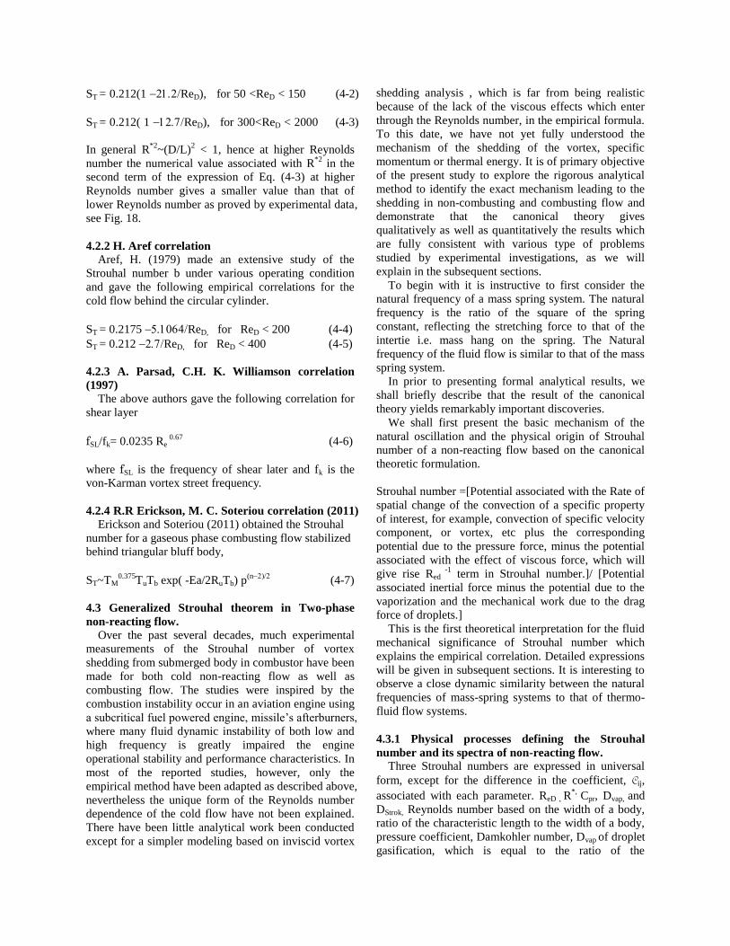
ST = 0.212(1 ReD), for 50 <ReD < 150 (4-2)
ST = 0.212( 1 ReD), for 300<ReD < 2000 (4-3)
In general R*2
~(D/L)2 < 1, hence at higher Reynolds
number the numerical value associated with R*2
in the
second term of the expression of Eq. (4-3) at higher
Reynolds number gives a smaller value than that of
lower Reynolds number as proved by experimental data,
see Fig. 18.
4.2.2 H. Aref correlation
Aref, H. (1979) made an extensive study of the
Strouhal number b under various operating condition
and gave the following empirical correlations for the
cold flow behind the circular cylinder.
ST = 0.2175 ReD, for ReD < 200 (4-4)
ST = 0.212 ReD, for ReD < 400 (4-5)
4.2.3 A. Parsad, C.H. K. Williamson correlation
(1997)
The above authors gave the following correlation for
shear layer
fSL/fk= 0.0235 Re 0.67 (4-6)
where fSL is the frequency of shear later and fk is the
von-Karman vortex street frequency.
4.2.4 R.R Erickson, M. C. Soteriou correlation (2011)
Erickson and Soteriou (2011) obtained the Strouhal
number for a gaseous phase combusting flow stabilized
behind triangular bluff body,
ST~TM0.375
TuTb exp( -Ea/2RuTb) p(n
(4-7)
4.3 Generalized Strouhal theorem in Two-phase
non-reacting flow.
Over the past several decades, much experimental
measurements of the Strouhal number of vortex
shedding from submerged body in combustor have been
made for both cold non-reacting flow as well as
combusting flow. The studies were inspired by the
combustion instability occur in an aviation engine using
a subcritical fuel powered engine, missile’s afterburners,
where many fluid dynamic instability of both low and
high frequency is greatly impaired the engine
operational stability and performance characteristics. In
most of the reported studies, however, only the
empirical method have been adapted as described above,
nevertheless the unique form of the Reynolds number
dependence of the cold flow have not been explained.
There have been little analytical work been conducted
except for a simpler modeling based on inviscid vortex
shedding analysis , which is far from being realistic
because of the lack of the viscous effects which enter
through the Reynolds number, in the empirical formula.
To this date, we have not yet fully understood the
mechanism of the shedding of the vortex, specific
momentum or thermal energy. It is of primary objective
of the present study to explore the rigorous analytical
method to identify the exact mechanism leading to the
shedding in non-combusting and combusting flow and
demonstrate that the canonical theory gives
qualitatively as well as quantitatively the results which
are fully consistent with various type of problems
studied by experimental investigations, as we will
explain in the subsequent sections.
To begin with it is instructive to first consider the
natural frequency of a mass spring system. The natural
frequency is the ratio of the square of the spring
constant, reflecting the stretching force to that of the
intertie i.e. mass hang on the spring. The Natural
frequency of the fluid flow is similar to that of the mass
spring system.
In prior to presenting formal analytical results, we
shall briefly describe that the result of the canonical
theory yields remarkably important discoveries.
We shall first present the basic mechanism of the
natural oscillation and the physical origin of Strouhal
number of a non-reacting flow based on the canonical
theoretic formulation.
Strouhal number =[Potential associated with the Rate of
spatial change of the convection of a specific property
of interest, for example, convection of specific velocity
component, or vortex, etc plus the corresponding
potential due to the pressure force, minus the potential
associated with the effect of viscous force, which will
give rise Red -1
term in Strouhal number.]/ [Potential
associated inertial force minus the potential due to the
vaporization and the mechanical work due to the drag
force of droplets.]
This is the first theoretical interpretation for the fluid
mechanical significance of Strouhal number which
explains the empirical correlation. Detailed expressions
will be given in subsequent sections. It is interesting to
observe a close dynamic similarity between the natural
frequencies of mass-spring systems to that of thermo-
fluid flow systems.
4.3.1 Physical processes defining the Strouhal
number and its spectra of non-reacting flow.
Three Strouhal numbers are expressed in universal
form, except for the difference in the coefficient, Cij,
associated with each parameter. ReD R*,
Cpr, Dvap, and
DStrok, Reynolds number based on the width of a body,
ratio of the characteristic length to the width of a body,
pressure coefficient, Damkohler number, Dvap of droplet
gasification, which is equal to the ratio of the
characteristic time of shedding of shedding of a specific
property of interest, such as vortex to that vaporization
time. DStrok is the ratio of the characteristic time of
shedding of a specific property of interest, such as
vortex to that of droplet relaxation time.
4.3.2 Spectra of Strouhal numbers of interest in two-
phase flow.
The Strouhal spectra of interest in thermo fluid flow.
(i) Strouhal number has been commonly addressed for
vortex shedding.
(ii) In general there are six types of spectra of Strouhal
number: (a) spectra of radial velocity component, (b)
spectra of azimuthal component (c) spectra of axial
velocity component. (d). spectra of thermal energy
shedding (e). spectra of mass shedding, (f). spectra of
chemical reaction at different Damkohler number.
The numerical value of each Strouhal number is
different for a given combustor operating condition.
Since the total number of these spectra of Strouhal
number in two-phase flow becomes exponentially large
such that the fluid is easily get into oscillation for any
given disturbance.
Each oscillation has specific intensity depending on
the parameters entering the Strouhal number.
Additionally for a flame stabilization, bluff body
stabilized flames are susceptible to thermo-acoustic
instability and this provoke further interest in the
combustion instability problem, as we shall discuss in
later section. When fluid oscillation is in resonant state
with the acoustic mode of the combustors natural
frequencies , including lateral, transverse or azimuthal
modes, the oscillation could be in resonant condition,
Furthermore if the oscillation satisfies the Reyleigh
criterion the combustion oscillation will be enhanced
and seriously impair the combustion process. It is
evident the large number of Strouhal spectra is one of
the great concern in combustion oscillation. We shall
discuss all the thermo chemical sources in oscillation
due to chemical-acoustic coupling in later section.
4.3.3 Strouhal number of mass shedding of a liquid
spray
A spray will also shed its mass at its own Strouhal
number, which is different from that of vortex. We
obtain the Strouhal number STM of mass shedding from
spray, STM
STM=ReDMTotal[(Cp)L]}ln(r/rS)∫∫T
{[(Cp)ln(T+r(Cp)ln(T+rs]}tanddz
ln(r/rS)∫∫∫T{ln(T+∂(Cp)/∂r)Tr}
dddzcos
ln(r/rS)∫∫∫T{∂[(Cp)ln(T+∂
ln(T+∂[(Cp)/r∂T
dddzcos
ln(r/rS)∫∫∫T{∂[(Cp)ln(T+∂zln(T+
∂[(Cp)/∂zTzdddzcos
+ln(r/rS)Kmn0V∫∫T Kmndddzcos
ln(r/rS)ReDCprPr∫∫∫T(urp/)/T
dddzcos
ln(r/rS)ReDCprPr∫∫∫T(uzp/z)/T
dddzcos
PrR*ln(r/rS)∫∫∫Tdddzcos
R*ln(r/rS)∫∫∫T
2∂[∂(Cp)rlnT
∂2∂lnT
∂∂(Cp)rr∂
TKm∂
+R*2
ln(r/rS)∫∫∫T {[∂(Cp)r[∂lnT∂z
2
∂ln(T∂z)∂(Cp)r∂z)dddzcos
ln(r/rS)∫∫∫dddzcosdddzcos
ln(r/rS)∫∫∫Kmnq]∂zdddzcosdddzcos
Cp/C
*)][∫∫∫T
r
2(
*C
*)
x∂2ln
*T∂∂
2ln
*T∂z
dddzcos
}
dddzcos
∫∫∫T
*ln(
*T )/tdddzcos
∫∫∫r2(
*C
*)[∂2ln
*T∂
(*C
*)∂2ln
*T∂z
dddzcos
+GReDS+DVapln(r/rS)∫∫∫∑njmj[(1TiTS)]
/T dddzcos
(Group combustion of a spray)
+ReDPrln(r/rS)∫∫∫TJTlnTdddzcos
ReDPr* ∫∫∫T
JT
* lnT
dddzcos
(Boundary layer stripping cpmbustion)
∫∫∫[r2(
*C
*)∂2ln
*T∂
(*C
*)∂2ln
*T∂z
dddzcos
{Pr ln(r/rS)∫∫∫T[/Cprp/dddzcos
ln(r/rS)∫∫∫{T[ln(T)]/dddzcos
+(CfDStork)Pr
ln(r/rS)∫∫∫∑njFj(uulk)]
’dddzcos
DChem Pr∫∫∫{ T
T
’ d ddzcos
Pr* Pr
∫∫∫lnT t}
’ d ddzcos
Pr
DChem∫∫∫{ T
T
’ d ddzcos
Pr∫∫∫T
lnT
t}
’ d ddzcos
(4-7)
We will provide a universal form of Strouhal number
in later section. In this expression we find that there are
major mechanisms that will provoke the mass shedding
at the natural frequency determined by the Strouhal
number. The effects of various convection and
conduction of various flow properties such as velocity
species, canonical entropy, conductive processes due to
viscosity and thermal and mass transport all take place
in three direction, two-phase effects including
vaporization drag force, viscous dissipation all of them
influence the shedding frequency. The intercoupling
among all the shedding processes are immensely
intercoupled. For example, the shdding of the velocity
in axial direction will affect all other shedding

processes. This is typical characteristic of non-linear
intercoupling mechanisms.
4.3.4 Dynamics and aerothermochemical structure
of a spray flow field;
We are concerned with the structure of the flow field
and the thermo-chemical performance characteristics of
practical interest. The flow field structure, including the
distributions of the density, velocity, vortex,
temperature, and the Strouhal number of flow
properties of interest will be examined in cylindrical
coordinate systems.
Continuity equation
∂∂t +●u =∑nj mj (4-8)
where the subscript j stands for the droplets with j-th
size class, and mj is the vaporization rate. The equation
can be rewritten as
∂ln∂t + ∂ln∂ =∑nj mj/∙u (4-9)
The equation can be integrated to give
1 = exp∫exp{t∑nj mj/∙u]}dtd(4-10)
where dudx + vdy
Momentum equation
Momentum equation of two-phase chemically
reacting flow is expressed by
∂u∂t + ∙uv = ∙p +∙∑nj mj (u uli)
∑nj Fj∫vu)injdy (4-11)
Three velocity components are formulated by the
canonical integration method in the following
acxiomatix expressions.
Radial component
Governing equation of the radial velocity component
in cylindrical coordinate is written as
∂(∂ur)/∂r2∂(ur
2)/∂r+ur∂(ur)/∂r+∂(/∂r)∂(ur)/∂r
∂(/∂t)u∂(u)/∂(du2/r+uZ∂(ur)/∂z
∂P∂rr)∂(rrr)/∂r∂(r∂ur)/∂r2r)∂(r/∂r)
∂(rZ)/∂z ∑njmj(uuli)∑njFjvu)inj
(4-12)
4.3.5 Theorem 5: Radial velocity component of a
spray flow field
Integrating the equation and non-dimensionalization
of the result gives the non-dimensional radial velocity
distribution,
u= u)∞
∫{[(∂u/∂(∂)/∂d
Re∫(u
2)(u2)rs]d’
Re∫∫ur∂(u)/∂d d’
ReST∫∫∂(u/∂) d d’
Re∫∫u∂(u)/∂(d d d’
Re∫∫(u2/ d d’
(Re)R* ∫∫[uZ∂(u)/∂z] d d
(CpRe) ∫∫(∂P∂ d d’
∫∫r)∂(r)/∂ ]d d’
∫∫∂(∂u)/∂2 d d
’
∫∫)∂(/∂) d d’
∫∫∂(Z)/∂z d d’
ReDSTDVap∫∫∑[njmj(uuli) d d’
+NCfReDSTDStork
)∫∫NCfReDSTDStork)∑njFjd’d
Re∫vu)injd
(4-13)
where ReD= U1D/R*
= L/D, ST= D/U1Shed, DVap
=Shed/Vap, DStork =Shed/Vap,
and dynamic viscosity at lN= number of
particles, Cf = mean droplet drag coefficient, CP =
pressure coefficient.
4.3.6 Strouhal number of radial velocity component
From the above equation, we obtain the Strouhal
number of radial velocity component of a spray flow
field in the following universal form, which applies to
all the natural frequencies,
STR [STR STR ReD-1
]/ STR(4-14)
where all the coefficients STRJ’s are given by
STR∫(u2)(u
2)rs]d∫∫ur∂(u)/∂dd
’
+∫∫u∂(u)/∂(d d d’∫∫(u
2/ d d
’
R*
∫∫[uZ∂(u)/∂z]d d’Cp ∫∫(∂P∂ d d
’
R*
∫∫[uZ∂(u)/∂z]d d’R
* ∫∫[uZ∂(u)/∂z]d d
’
(4-15)
ST∫{[(∂u/∂(∂/∂du)∞ur)S]
∫∫r)∂(r)/∂]dd’∫∫∂(∂u)/∂2dd’
∫∫)∂(/∂)dd ∫∫∂(Z)/∂z d d’}
(4-16)
STR∫∫∂(u/∂)dd’
∑kDVapk∫∫∑[nkmk (uulk)dd’
NCfkDStorkk)∫∫∑nkFk, dd
(4-17)
From the analytical result we found the following facts;
Strouhal number =[Potential associated with the Rate of
spatial change of the convection of a specific property
of interest, for example, convection of specific velocity
component, or vortex, etc plus the corresponding
potential due to the pressure force, minus the potential

associated with the effect of viscous force, which will
give rise Red -1
term in Strouhal number.]
/[Potential associated inertial force minus the potential
due to the vaporization and the mechanical work due to
the drag force of droplets. ]
This is the first theoretical interpretation for the fluid
mechanical significance of Strouhal number which
explains the empirical correlation. Detailed expressions
will be given in subsequent sections. It is interesting to
observe a close dynamic similarity between the natural
frequencies of mass-spring systems to that of thermo-
fluid flow systems.
4.3.7 Azimuthal velocity component
Momentum equation of azimuthal velocity
(1/r)2[∂2(∂u)/∂∂(u
2)/r∂ur(∂u/∂r
u∂(u/r∂(1/r)uuruz∂(u/∂z
ReST∂(u/∂t)
ReR*-1∂P∂r))[∂()/∂∂(∂u)/∂
r2))[∂(r
2r)/∂
∂(z)/∂z]
∑[njReDSTDVap]njmj(uuli)
NCfReDSTDStork)∑njFj
(4-17)
4.3.8 Theorem 6: Azimuthal velocity distribution By integrating and non-dimensionallizing the
momentum equation gives
u
(u)0∫u∂∂)/∂d
∫∫∫[∂2(∂u)/∂
d
ReD∫∫∫∂(u2)/∂
d
ReD ∫∫∫(ur∂u/∂d
d
+
ReD∫∫∫uur)/d
d
ReD∫∫∫u∂(u/∂d
d
ReD ∫∫[uud
+
ReDR*
∫∫∫uz∂(u/∂zd
d
Cp ReD∫∫∫∂P ∂d
d
∫∫∫∂(
2r)/∂r
d
∫∫[∂()/∂
d
∫∫1/2) ∫∫[∂(∂u)/∂
d
∫∫
2)[(∂ur/∂
d
∫∫ ∂(z)/∂zd
ReDSTDVap∫∫∑[njmj(uuli)
d
+NCfReDSTDStork
)∫∫NCfReDSTDStork)∑njFjd
Re∫vu)injd
(4-18)
4.3.9 Strouhal number for the shedding of the
azimuthal velocity component
From the above equation we formulate the Strouhal
number for the azimuthal velocity component is given
by the universal form,
ST [ST ST ReD-1
]/ ST(4-19)
where all the coefficients are given by STj are given by
STR∫(u2)(u
2)rs]d∫∫ur∂(u)/∂dd
’
+∫∫u∂(u)/∂(d d d’∫∫(u
2/ d d
’
R*
∫∫[uZ∂(u)/∂z]d d’Cp ∫∫(∂P∂ d d
’
R*
∫∫[uZ∂(u)/∂z]d d’R
* ∫∫[uZ∂(u)/∂z]d d
’
(4-20)
ST∫[(∂u/∂(∂/∂du)∞ur)S]
∫∫r)∂(r)/∂]dd’∫∫∂(∂u)/∂2 d d’
∫∫)∂(/∂)dd ∫∫∂(Z)/∂z d d’}
(4-21)
STR∫∫∂(u/∂)dd’
∑kDVapk∫∫∑[nkmk (uulk)dd’
NCfkDStorkk)∫∫∑nkFk, dd
(4-22)
Again the physical mechanism for the Strouhal number
follows the same principle described earlier.
4.3.10 Axial velocity component
4.3.10.1 Momentum equation of axialvelocity Momentum equation for the axial velocity
component is given by
∂(∂uz)/∂z2∂(uz
2)/∂z
=∂(uz/∂t) + uz∂(uz)/∂z +ur∂(uz/∂r)
∂P∂zr)∂(rrz)/∂r+r)∂(rz/∂)
∂(ZZ)/∂z∂ln∂z∂(∂uz∂z)]
(∂∂z)(∂uz)/∂z)vuz)inj
∑[njReDSTDVap]njmj(uzuzi)
NCfReDSTDStork)∑njFjz
(4-22)
Integrating the equation gives the velocity distribution.
uz=z-1uz)Z=0 z
-1RED∫(uz
2)∞(uz
2)z]dz
z-1
RED∫∫uz∂(uz)/∂zdzdz
z-1
RED∫∫ur∂(uz/∂r) dzdz
z-1
Cp RED∫∫∂P∂zdzdz
(R*2
)∫∫)∂(z)/∂] dzdz
+z-1
(R*2
)∫∫[ )∂(z/∂)] dzdz
z-1
(R*2
)∫∫∂(r/∂z)]dzdz
z-1
RED∫∫∂(ZZ)/∂z
∂ln∂z∂(∂uz∂z)]dzdz
z-1
RED R*-1
∫vu)injdz
(4-23)
4.3.10.2 Strouhal number for the shedding of
velocity component in z-direction

The universal form of the Strouhal number is given
by
STZ [STZ STZ ReD-1
]/ STZ(4-24)
where the coefficients are expressed by
STZ0=∫(uz2)∞(uz
2)z]dz∫∫uz∂(uz)/∂zdzdz
∫ur∂(uz/∂) dzdzCp∫∫∂P∂zdzdz
(4-25)
STZ1=[(R*2
)∫∫)∂(z)/∂] dzdz
+ (R*2
)∫∫[ )∂(z/∂)] dzdz
(R*2)∫∫∂(r/∂z)]dzdz∫∫∂(ZZ)/∂z
∂ln∂z∂(∂uz∂z)] dzdz]
z-1RED R*-1∫vu)injdz (4-26)
STZ2=∫∫{∂(uz/∂) dzdz
∫∫∑[njDVap]njmj(uzuzi) dzdz
NCfkDStorkk)∫∫∑nkFk, dd
(4-27)
4.3.11 Vortex distribution in a liquid spray flow field
By formulating the vortex equation in a cylindrical
coordinate and by applying the canonical integration we
obtain an axiomatic representation of the vortex
distribution in a spray flow field,
4.3.12 Theorem 7: Vortex distribution
1ReD
∫uud
ReD∫(∂v∂)ddRe
*2∫∫∂[∂∂
)dd
CPr ReD∫∫(∂P∂)(∂ln∂)ddv
+ ∫∫r)∂(rrz)/∂r]dd+
∫∫r)∂(rz/∂) dd
ReD-1∫∫∂(ZZ)/∂z∂ln∂z∂(∂uz∂z)]] dd
RED R*-1
∫vu)injdz/STZ RED∫∫(∂∂)dd
∑[njjDVap.k ∫∫∑njmj(liz) dd
∑njjDVap.k∫∫[(x∑njm)(uul)dd[njCfjDStork]
∑[njCfjDStork∫∫∑(nkxFk)dd
∑[njCfjDStork∫∫∑njFjz dd
Cf∫∫∑nj[(∂Fj∂)(∂Fj∂)]dd
(4-28)
4.3.12 Theorem 8: Strouhal number for vortex
shedding in a spray flow field
From the above equation we obtain the following
expression of the Strouhal number of vortex shedding
for two-phase chemically reacting flow in universal
form.
ST [ST ST ReD-1
]/ ST(4-29)
ST∫uud∫(∂v∂)dd(4-30)
STReD-1[0]Re
*2∫∫∂[∂∂
)dd]
CPr∫∫
(∂P∂)(∂ln∂)ddv
∫∫r)∂(rrz)/∂r]dd∫∫r)∂(rz/∂)dd
∫∫ ∂(ZZ)/∂z∂ln∂z∂(∂uz∂z)]]dd
(4-31)
ST∫∫(∂∂)dd∑[njjDVap.k ∫∫∑njmj(liz) dd]
∑njjDVap.k∫∫[(x∑njm)(uul)dd[njCfjDStork]
∑[njCfjDStork∫∫∑(nkxFk )dd
∑[njCfjDStork∫∫∑njFjz dd
Cf∫∫∑nj[(∂Fj∂)(∂Fj∂)]dd
jDVap.k∫∫∑nj [(x∑njm)(uul)dd
(4-32)
4.3.13 Experimental validation
There have been number of experimental correlation
of Strouhal number. Some representative experimental
correlations are shown
(1) Strouhal number of vortex shedding Lienhard, 1966, Aehenbach and Heineeke 1981 gave
the following correlation of Strouhal number with
Reynolds number
ST [ST ST ReD-1
]/ ST(4-33)
ST/ ST and ST/ ST for 40<RD< 200
(2) Dynamics of bi-modal vortex shedding;
Chiu’s conjecture Sakamoto, and Kitami (1980) reported that the vortex
shedding from the cylindrical body has two modes. The
regular vortex, Karman vortex as high mode and on the
other hand there is a lower mode vortex shedding
processes. They attributed that the lower mode is
caused by the pulsation of vortex sheet separated from
the surface are in the turbulent wake with progressive
motion respectively. The nature of the progressive
motion was neither qualitatively nor quantitatively
clarified. Review of the literature reveals no well
accepted mechanism for the wakes progressive motion.
However, we have made a quantitative description that
the location of the separation and reattachment points
are oscillating and cause the length of the recirculation
zone to oscillate .see Fig.9 For example we estimated
that the width of the recirculation zone oscillate at the
speed given by Ulw=2DQS RED R*-1
STZlw/Shed .
The periodical change in the separation and
reattachment and the length and the width of the wake
bring out major wake periodic motion. This periodic
motion certainly influences the vortex shedding. The S
shedding of Karman vortex street usually assume that
the wake region is stationary hence we get a clear
undisturbed frequency for the vortex shedding, however
when the wake is in oscillatory motion as described the
frequency of the wake oscillation will certainly
introduce secondary Strouhal number. It is conjectured
the lower mode is the result of the wake oscillation.
This conjecture though physically sound would require
experimental validation. The experimental data of
Strouhal number of vortex shedding shedding from
sphere and other types of bodies by Sakamoto Kitami
(1980), Bearman (1989), Okajima (1982), Reinstra
(1983), Perry etal. (1982), and Sheard etal. (2003) are
shown in Fig.18. These data are quite consistent
qualitatively.
4.3.14 Normalized shear layer frequency
The natural frequency of shear layer fShea /fk is
correlated with that of Karman vortex sheddding
frequency fk. Results indicate that the ratio increases
linearly with logarithm of Reynolds number.
4.3.14.1 Theorem 9: Temperature distribution in
spray flow field By using canonical integration of the energy equation
we obtain the following temperature distribution.
(T+)u
[u)(T+)S
R*-1u
∫∫[∂uz,I T+)∂id
CPrR*-1u
∫∫[(uz∂pi∂)]idd
CPrR*-1u
∫∫[(u∂pr∂idPr∫∫idd
R*-1u
∫{TInjTS)(injvinj,i )]i}d
(PrReu
PrRDu
∫∫∂[(Cp) ∂ T+)∂∂id d
PrRD
R*
u∫∫∂[(Cp) ∂ T+)∂z
2]d d
+u
[(Cp)(Ti+)(Cp)(Ti+)s]i
(4-34)
4.3.14.2 Theorem 10: Strouhal number for thermal
energy shedding
By proper algebraic steps we obtain the Strouhal
number for thermal energy shedding
STTherm=[u)(T+) [u)(T+)S
R*-1∫∫[∂uz,I T+)∂id
CPrR*-1∫∫[(uz∂pi∂)]idd
CPrR*-1∫∫[(u∂pr∂idPr∫∫idd
R*-1∫{TInjTS)(injvinj,i )]i}d
(PrRD
[(Cp)(Ti+)(Cp)(Ti+)s]i
PrRD
∫∫∂[(Cp) ∂ T+)∂∂id d
PrRD
R*
∫∫∂[(Cp) ∂ T+)∂z2]dd
∫∫[∂T+)∂ddCPr∫∫(∂pi∂dd
DChem∫∫dd
DVapV∫∫[∑njmj (1TTS)]idd
CfPr-1
DStork V∫(∑njFj(uul))]idd
(4-35)
Investigation of the Strouhal numbers of three velocity
components, radial, azimuthal and axial direction in
cylindrical coordinate two-phase chemically reacting
flow, can be presented in the following five parametric
Strouhal number.
4.3.14.3 Summary
Strouhal numbers of velocity components
STr=[(C0rC1rRED-1RED
-1 R
*2 C2rC3rCP]
/[( B0r B1rNDVap B2rNCfDStork)]
(4-36)
ST=[(C0CRE-1RED
-1R
*2C2C3CP]
/[( B0B1NDVap B2NCfDStork)]
(4-37)
STZ=[(C0zC1zRED-1R
*2 RED
-1 C2ZC3zCP]
/[( B0zB1zNDVap B2zNCfDStork)]
(4-38)
Strouhal number of vortex shedding
ST=[(C0C1 RED
-1C2 R
*2 RED
-1C3 CP]
/[(B0 B1 NDVap B2 zNCfDStork)]
(4-39)
Strouhal number of thermal energy shedding
STherm=[(C0C1h RED-1C2h R
*2 RED
-1C3h CP]
/[(B0h B1h NDVap B2hNCfDStork)]
(4-40)
4.3.15 Basic dynamic features of Strouhal number 1.
Non-reacting flow
We conclude that all the family of Strouhal number
in two-phase chemically reacting flow can be expressed
by a universal formula. Basic features of Strouhal
numbers are remarkably unique, as shown in the above
equation.
(1) Strohal number of dynamic properties such as
velocity, vortex are characterized by five
parameters, RED R* CP DVap and DStork.
(2) RED represents the ratio of dynamic head to the
viscous force. Reynolds was the first to point this
aspect in 1900.
(3) R* is the ratio of the characteristic length to the
width of the body constitute the “blockage effects”
of the body of the flow field, which in turn affect
the drag force and subsequently the Strouhal
number, West and Apelt (1982), made an extensive
measurement of the effects of blockage of various
aspect ratio of a cylinder.
Blockage effect has been experimentally measured
with following empirical formula.
CDC/CD=1/(1 +CPC)/CP) (4-41)
n2./12)B
2 +(CD/4)B (4-42)
B is the blockage in %. CD is the drag coefficient, CP is
pressure coefficient, and subscript “c” is the corrected
value. The experimental results indicated that for a
body with diameter of 32 mm has the blockage of 25%
and for 41 mm the corresponding B is 16%.
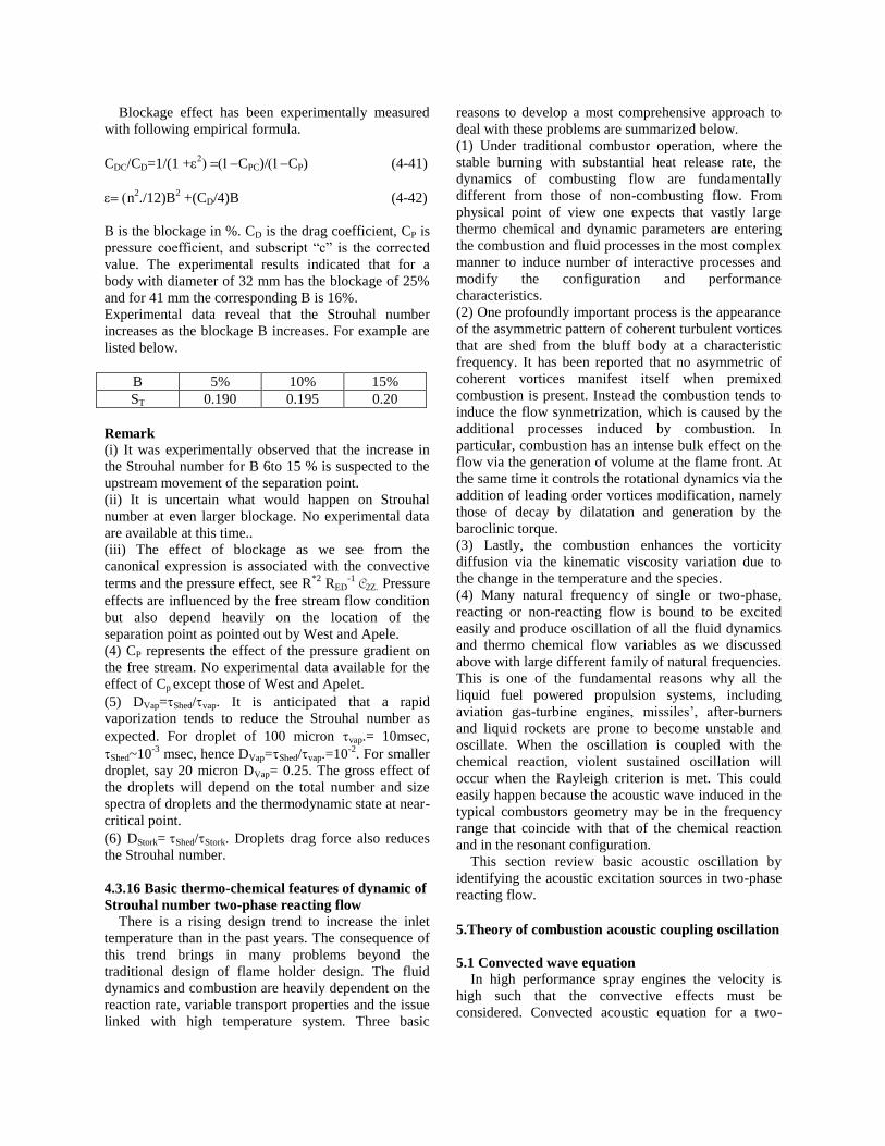
Experimental data reveal that the Strouhal number
increases as the blockage B increases. For example are
listed below.
B 5% 10% 15%
ST 0.190 0.195 0.20
Remark
(i) It was experimentally observed that the increase in
the Strouhal number for B 6to 15 % is suspected to the
upstream movement of the separation point.
(ii) It is uncertain what would happen on Strouhal
number at even larger blockage. No experimental data
are available at this time..
(iii) The effect of blockage as we see from the
canonical expression is associated with the convective
terms and the pressure effect, see R*2
RED-1
C2Z. Pressure
effects are influenced by the free stream flow condition
but also depend heavily on the location of the
separation point as pointed out by West and Apele.
(4) CP represents the effect of the pressure gradient on
the free stream. No experimental data available for the
effect of Cp except those of West and Apelet.
(5) DVap=Shed/vap. It is anticipated that a rapid
vaporization tends to reduce the Strouhal number as
expected. For droplet of 100 micron vap.= 10msec,
Shed~10-3
msec, hence DVap=Shed/vap.=10-2
. For smaller
droplet, say 20 micron DVap= 0.25. The gross effect of
the droplets will depend on the total number and size
spectra of droplets and the thermodynamic state at near-
critical point.
(6) DStork=Shed/Stork. Droplets drag force also reduces
the Strouhal number.
4.3.16 Basic thermo-chemical features of dynamic of
Strouhal number two-phase reacting flow
There is a rising design trend to increase the inlet
temperature than in the past years. The consequence of
this trend brings in many problems beyond the
traditional design of flame holder design. The fluid
dynamics and combustion are heavily dependent on the
reaction rate, variable transport properties and the issue
linked with high temperature system. Three basic
reasons to develop a most comprehensive approach to
deal with these problems are summarized below.
(1) Under traditional combustor operation, where the
stable burning with substantial heat release rate, the
dynamics of combusting flow are fundamentally
different from those of non-combusting flow. From
physical point of view one expects that vastly large
thermo chemical and dynamic parameters are entering
the combustion and fluid processes in the most complex
manner to induce number of interactive processes and
modify the configuration and performance
characteristics.
(2) One profoundly important process is the appearance
of the asymmetric pattern of coherent turbulent vortices
that are shed from the bluff body at a characteristic
frequency. It has been reported that no asymmetric of
coherent vortices manifest itself when premixed
combustion is present. Instead the combustion tends to
induce the flow synmetrization, which is caused by the
additional processes induced by combustion. In
particular, combustion has an intense bulk effect on the
flow via the generation of volume at the flame front. At
the same time it controls the rotational dynamics via the
addition of leading order vortices modification, namely
those of decay by dilatation and generation by the
baroclinic torque.
(3) Lastly, the combustion enhances the vorticity
diffusion via the kinematic viscosity variation due to
the change in the temperature and the species.
(4) Many natural frequency of single or two-phase,
reacting or non-reacting flow is bound to be excited
easily and produce oscillation of all the fluid dynamics
and thermo chemical flow variables as we discussed
above with large different family of natural frequencies.
This is one of the fundamental reasons why all the
liquid fuel powered propulsion systems, including
aviation gas-turbine engines, missiles’, after-burners
and liquid rockets are prone to become unstable and
oscillate. When the oscillation is coupled with the
chemical reaction, violent sustained oscillation will
occur when the Rayleigh criterion is met. This could
easily happen because the acoustic wave induced in the
typical combustors geometry may be in the frequency
range that coincide with that of the chemical reaction
and in the resonant configuration.
This section review basic acoustic oscillation by
identifying the acoustic excitation sources in two-phase
reacting flow.
5.Theory of combustionacoustic coupling oscillation
5.1 Convected wave equation
In high performance spray engines the velocity is
high such that the convective effects must be
considered. Convected acoustic equation for a two-

phase combusting flow was formulated by Chiu and
Summerfield (1974) and is given by
D2[ln(p/p0)Dt
2]∙[af
2 ln(p/p0)]
=∂ui/∂xj)/∂uj/∂xi) +D( ) (5-1)
where
∑ hi )/CpT∑∑xiDai/wiDa)(ui uj)+u
+∙(CpT)Chem=1
+DVapV∫∫[∑njmj (1TTS)]idd
CfPr-1
DStork V∫(∑njFj(uul))]idd
(5-2)
where afis the isentropic speed of sound,L/Q,
DVap=Shed/Vap, DStork=Shed/Stork
Chem=1
=PrSTRDDa Vis the rate of change in the
spray volume. This is the burning rate divided by the
liquid fuel density.
5.2 Major acoustic
( )
D( ) {∑ } YiVihi
RTxiDai/wiDa)(ui uj)+u
+∙(CpT)Chem=1
niFi/Sti(uuli)/Q +invin(Cp)(TTl)in
(5-3)
{∑ hi}Dt= PrSTRDDChem(Chem=1
’Dt
=PrSTReDa Chem=1
{T’/T)]/[1iT)
j]
+ (1/2)[i +T’/T)iI
’/I)]}/Dt
(5-4)
Chem=1
is the steady state reaction rate.’is the non-
dimensional fluctuating reaction rate.
5.3 Chemical-acoustic driving sources: Gas-phase
premixed combustion in spray and/or gaseous fuel
combustion
Chemical reaction driving sorce
We will adapt a one-step chemical reaction rate
expressed by
N
j
j
kj
TR
PX
TR
EBT
100
',
exp
(5-5)
By taking account of the fluctuation in temperature,
pressure and the concentration of species, we obtain the
following rate of the fluctuating reaction for the
gaseous–phase combustion. TSand I0 are Lagrange
multiplier for temperature and j-th chemical spices, and
pressure fluctuation is given by
p’/p=(
’T
’/T) (5-6)
TZ is the temperature expressed in Zeldovich form.
{ {∑ hi}Dt}CHEMp’
=S11TZ’2 (S12 S13TZ
’
’)+S14(TZ
’i
’ (5-7)
S11=(chem)/T)2][1iTZ)
j]} (5-8)
S12=chem) {/TZ)] /[1iT)j
] } (5-9)
S13=chem )(1/2)[( /[T)] } (5-10)
S14=chem) (1/2)[(T)i)]-1
} (5-11)
wherechem) is the steady state reaction rate. 5.4 Liquid fuel combustion evaporation–pressure
coupling for acoustic driving sources
D( ) T’) [(
’T
’/T)]
+DVapV∫∫[∑njmj (1TTS)]i[(’T
’/T)]dd
CfPr-1
DStork V∫(∑njFj(uul))]i[(’T
’/T)]dd
+(invin)’(CpT)in [(
’T
’/T)]
(5-12) 5.5 Two-phase acoustic coupling sources
D( ) DVap V S21vapT’)
2
+ DVap V S22’T
’)+DVap V S23(( ’
)
+DVap V S24 T’)+CfPr
-1DStork V S25
’ (u
’uli
’)
+CfPr-1
DStork V S26T’(u
’ul
’) + S27
’ S28T
’
(5-13)
where S2i are given by
S21= nimi)/T, S22=nimi)(5-14)
S23nimi)’/[1TTS)](5-15)
S24nimi)[1TTS)/T)] (5-16)
S25=niFiQ(5-17)
S26=niFi)’(uuli)/Q(5-18)
S27 = (invin)(CpT)in (5-19)
S28 =(invin) /T (5-20)
We observe that there are three characteristic times
enter in the acoustic driving sources.
(I) Chemical reaction time or Damkohler

number. The magnitude depends on the
type of fuel operating environment,
mixture ratio. In case of premixed flame
in spray, the magnitude of premixed
combustion depends on time and space.
The chemical-acoustic driving gives the
high frequency oscillation of the order of
KHz.
(II) Vaporization time. Here we are talking
about the typical spray evaporation time,
which will be different from that of
single droplet because of the group
effects’
(III) Two-phase relaxation time, which is also
different from that of a single droplet. It is anticipated that the two-phase vaporization, non-
premixed combustion and droplets dynamics create low
frequency oscillation. High frequency flamlet
oscillation can possibly drive the acoustic oscillation. It
conjectured that the pressure oscillation is frequently
provoked by rapid heat shedding to induce local
burning rate, hence of the burning rate oscillation is
sufficiently rapid in flamlets, and acoustic wave may be
triggered.
5.6 Table of the sources of acoustic-two-phase
reacting flow oscillation
Acoustic oscillation in two-phase reacting flow in
driven by the following sources, which are proportional
to the products of two coupled fluctuating variables
listed below.
Coupling
sources
Chemical-
acoustic
Two phase
acoustic
Injection-
acoustic
T’2
S11 S21va 0
’T
’ S12+ S13 S22vap 0
’i
’ S13
T’ 0 S24vap 0
’ 0 S23vap 0
’(u’ ul
’) 0 S25/Sti 0
T’(u’ ul
’) 0 S26/Sti 0
’ 0 0 S27
T’ 0 0 S28
p0 is the reference pressure, a is the frozen speed of
sound,us the viscous dissipation. The equation is a
non-linear and is suitable for the investigation of strong
oscillation, where the non-linear effects are important in
high supersonic and hypersonic flow and explosion
phenomena. Most of the classical analysis employs
linearized approximation to ease the analysis.
In the following analysis we will assume linearized
approach to deal with the acoustic-chemical reaction
coupled acoustic oscillation in a cylindrically shaped
combustor.
5.7 Theory of combustionacoustic coupling for high
frequency oscillation The one step chemical reaction rate is expressed by
’=ST
’/T)]/[1iT)
j]
+(1/2)[i’ +T
’/T )
iI’/I)]
(5-21)
The pressure fluctuation is given by
p’/p=(
’T
’/T) (5-22)
The temperature fluctuation is
T=TQCP (5-23)
TZ is the Zeldovich temperature these two descriptions
will be used for the prediction of chemistry-acoustic
coupling and thereby predicting the Reyleigh criterion
of combustion stability.
We observe that there are three characteristic times
enter in the acoustic driving sources.
(IV) Chemical reaction time or Damkohler
number. The magnitude depends on the
type of fuel operating environment,
mixture ratio. In case of premixed flame
in spray, the magnitude of premixed
combustion depends on time and space.
The chemical-acoustic driving gives the
high frequency oscillation of the order of
KHz.
(V) Vaporization time. Here we are talking
about the typical spray evaporation time,
which will be different from that of
single droplet because of the group
effects’
(VI) Two-phase relaxation time, which is also
different from that of a single droplet. It is anticipated that the two-phase vaporization, non-
premixed combustion and droplets dynamics create low
frequency oscillation. High frequency flamlet
oscillation can possibly drive the acoustic oscillation. It
conjectured that the pressure oscillation is frequently
provoked by rapid heat shedding to induce local
burning rate, hence of the burning rate oscillation is
sufficiently rapid in flamlets, acoustic wave may be
triggered.
6. A review of spray combustion 1930 to 2013

6.1 1930- 1990
Research in spray combustion started in early 1930
by Tanazawa and Nukliyama in Japan on the
characterization of the atomization of liquid, in
particular on the classification of droplet size
distribution produced by various type of atomizer. The
study was actively continued in US notably by Lefebvre,
A.H., 1989, Chigier, N.A. 1981 Chigier, N.A. 1976.
In 1950’s Spalding and Godsave examined the
combustion behavior of a droplet in quiescent
atmosphere and developed a burning rate model. D2 law
was developed to aid in the practical calculation. In this
period much of the studies were focused on various
aspects of single droplet vaporization and combustion
which was continued to cover broad ranged fluid
dynamics and combustion characteristics. Notably by
Sirignano and his associates, see Sirignano 1983 and
1999, for related articles contained in the review and
the book, who developed extensively the droplet theory
including the effects of internal recirculation variable
properties and established a well, accepted film model
which has been widely used in spray calculation. In due
time microgravity experiments were carried out by
Kumagai in Japan who used the falling tower to
simulate the micro-gravity environment to eliminate the
buoyancy effect on the droplet combustion, for the first
time in 1950 This was to be followed by extensive
experimental program by F, William and Dwyer in
falling towers and in space shuttle, to validate the single
droplet theory, Falling tower experiments were to be
continued in Hokkaido Japan and China. The studies
found that the droplet combustion exhibits unsteady
behavior in transient period, and various problems such
as ignition and extinction behavior, While much
physical phenomena have been successfully obtained to
understand the detailed behavior of a droplet,
combustion. However the single droplet theory was
found to be unable to deliver a physically acceptable
combustion process and burning rate of a practical
spray. The theory gives an unreasonably rapid burning
rate, when it is used to predict the overall burning rate
of a spray, even for a dilute spray by several factors
faster than real spray. In order to circumvent this
shortcoming, In 1971, and the following few decades
Chiu and associates further extended the group
combustion model of a droplet cloud of spherical
configuration, to account for the effects of collective
interaction among droplets, and predicted the
combustion behavior. They found that a droplet in
spray does not burn as Spalding theory offered. Instead
the droplets vaporize in the spray to produce a fuel
vapor, which was then diffused outwardly to mix with
air and burn as a large envelope flame wrapping the
droplet cloud. The model was extended to the laminar
flow spray by Chiu and Kim and turbulent spray by
Chiu and Zhou used turbulence model in 1970 to
1980 to examine the combustion behavior and the
combustion modes including external sheath
combustion, external and internal group combustion
and drop wise combustion depending on
The magnitude of the group combustion number,
which describes the intensity of the collective
interaction, is expressed by the ratio of the vaporization
rate to that of oxidizer penetration into the cloud. The
numerical results carried out in a range of Reynolds
number of practical interest were found qualitatively
and quantitatively agree with experimental result. The
first experimental observation of the droplet behavior in
spray was independently carried out by Chigier and
McCreath (1974) who first time reported that the
droplet in a spray does not burn as Spalding and
Godsave described.
Chigier’s experiment (1974) confirmed the result of
the group combustion of many droplet systems
including spray. A most comprehensive experimental
verification of the group combustion in particular the
excitation of four group combustion mode was
validated for the first time by Mistune, Akamatsu, in
1980’s, see for example, Mizutani, Y., Akamatsu, F.,
Katsuki M., Tabata, T., and Nakabe K. (1996), and their
associates in Osaka Japan. attempted to evaluate the
combustion mechanism of each droplet cluster
downstream of the premixed spray flame simultaneous
time-series experiments by using an optical
measurement system consists of laser tomography,
MICRO, and PDA. In addition the group combustion
number of the spray was determined by the
experimental data. The laser image of droplet cluster
and time series data were found to be quite consistent
both temporary and spatially and a correlation existed
between the OH chemiluminescence and the CH band
light emission. The experimental results on the
excitation of various group combustion modes were
found to be in excellent agreement with the result of
group combustion theory. It may be added that the
spray experiment was carried out in Osaka University
by Mizutani, who was the thesis advisor of Akamatsu.
According to Mizutani, whom I met in Japan during my
key note lecture in Nagoya, Mizutani informed me that
he found the spray have a combustion behavior which
is similar to that of diffusion flame, however, Mizutani
was unable to explain the mechanism behind this
behavior. It is my feeling that what Mizutani found
must be the group combustion. This is an interesting
historical episode in the spray combustion. I was
unaware of the Mizutani’s experiment until I met him
in 1980,s well after the development of the group
combustion theory in 1971.In subsequent few decades,
various works on the goup combustion of droplet arrays,
clusters, droplet streams were carried out to examine
the effects of short range interaction of droplets on the

combustion behavior were carried out by Labowsky
(1978), Twardus and Bruzustowski (1977), and
Umemura (1981), on the combustion of droplet pair.
Bellan and her associate (1983) have extensively
studied the droplet cluster with finite sized droplet to
remedy the shortcoming of the point droplet model.
Additionally Sirignano and his associates (see
Sirignano (1999) and the references therein) have
carried a series of numerical simulation of droplets in a
moving stream to examine the detailed fluid dynamic
behaviors including velocity temperature and vortex
distributing to identify the effects of convective motion
and to remedy the traditional potential theory based
results of various studies n made, in which the effects
of rotational motion due to the vortex motion has been
largely ignored. The presence of the vortex and the
wake behind the droplet as well’s the internal
circulation were found to influence the droplet
combustion and micro-fluid flow. Dunn-Rankine
(2011), studied a collection of moving droplets
following one behind the other. Such stream has
sufficient organization and structure to allow detailed
probing by variety of experimental method to study the
effect of collective behavior. Aggaarwal had
extensively studied the ignition of droplets arrays and
sprays since 1980 to 2011 (see Aggaarwal (2011) and
the references cited therein). An impressive study of the
group combustion of coal particles were conducted by
Annamalai, K, (see Annamalai, K and Puri, K. (2007),
and the references therein ) in 1970 to 1990 to aid in the
application of the pulverized coal combustion and
gasification. The group combustion behavior was
qualitatively similar to that of liquid droplets. In
addition to the numerical simulation which were
extensively carried out in many countries including US,
Europe, Russia and Asia, many microgravity
experiment were carried out notably by Hokkaido
University by Ito and his Associates. During 1970
to1990 number of many droplet systems including
droplet array, streams, clusters and sprays have been
carried out. While exact number of papers a is not
known, however, the order of magnitude of the
published articles, technical conference papers and
reports as well as PhD and master thesis is well above
in the ramnge of fe w 103.
6.2 Progress and accomplishments of spray
combustion in 1990-2013
6.2.1 Candel, Lacas, Darahiba and Rolon (1999)
Candel, Lacas, Darahiba and Rolon (1999) conducted
extensive experimental study of spray combustion and
concluded that the group combustion is widespread and
consists a central problem. They found that the flame
structure features a vaporization front and active flame
front separated by a small distance exhibiting external
group combustion behavior in the simple geometry.
They estimated the group combustion number of
various type of configuration, and also indicated the
type of flame configuration in a range of group
combustion number, see Figs. 1 and 2. They found that
the ignition of droplet clouds in hot oxidizer
environment a dense spray, symbolizing group
vaporization reveals the possible ignition regimes and
provides description of the dynamics of the process.
The authors reported that the spray formed in a shear
conical injector fed with liquid x oxygen and gaseous
hydrogen. The flame established in this configuration
has been was examined extensively by with a variety of
optical diagnostics and image processing methods. The
data indicate that a high corrugurated flame
surrounding the dense spray of droplets formed by the
liquid core break-up. The effects of turbulence made
spray flame as a thick shell surrounding the LOX
sprays and oxygen vapor, see Fig. 3.
6.2. 2 Revellion and Vervisch (1999) Revellion and Vervisch (1999), reported a DNS
simulation by accounting the spray vaporization in
turbulent combustion modeling. The authors have
elected the case study limited to the problems observed
in external group combustion around the clusters of
droplet sprays. See Fig. 4. The authors adapted DNS to
simulate a dilute spray for the investigation of the
vaporization terms in the transport equation for Z”2.
Analytical results are utilized to derive an expressi9n
for the conditional mean value. One Droplet Model
(ODM) was compared with the DNS data. The paper
addressed on the turbulent spray combustion. Droplets
of fuel were injected in a two dimensional double wake
configuration and a flame is stabilized on the liquid jet
while simple step reaction process is used. A diffusion
flame develops and its main flame a is attached to the
spray by a triple flame consists of a rich premixed
flame where the droplets are vaporizing and two lean
premixed flame on the both sides of the jets Fig 5. The
vorticity field reveals heat release affects the flow
through gas expansion even at the end of the core of
spray.
The authors reported number of interesting results
including the time evolution of the fluctuation of the Z” 2 and compared the ODM with DNS. The results are
found to be in good agreement. The numerical results
indicated that despite of the large number of physical
parameters embedded in liquid fuel combustion, DNS
emerge as an effective tool to the study of turbulent
spray combustion.
6.2. 3 Pitsch (2006) Recently the Eulerian flamlet model was developed
by Pintsnh (2006). The flamelet equations are
reformulated in as an Eulerian form ,which leads to a
full coupling with the LES solver and thus facilitate the

consideration of the resolved fluctuation of the scalar
dissipation rate in the in the combustion model, see Fig.
6. The results from large eddy simulation of Pitsch
(2002), (solid curves) and the Lagrangian flamelet
model by Barlow and Frank (1998), dashed lines are
compared as show in Fig. 6. Temperature distribution
on the left scalar dissipation on the center and mixture
distribution, conditioned average of temperature, and
mixture fractions of NO, CO and H2 at x/D =30. Judging
from the each distribution one identify that the
combustion is in external group combustion mode, in
full agreement with that of Candel, Lacas, Darahiba and
Rolon (1999) and , Revellion and Vervisch (1999).
6.2.4 Erickson and Soteriou (2011)
When the reactant temperature increases the fluid
dynamic and combustion structure becomes from low
amplitude, broadband coarsely symmetric behavior to a
high amplitude tonal and asymmetric one that is similar
to the corresponding non-reacting flow. These
phenomena are caused by the fact that the reactant
temperature increases (i) the temperature ratio across
than flame is reduced and reduces the extent of
exothermiicity, and (ii) ths flame speed increases
causing the flame to propagate away from the bluff
body wake. In both cases the ability to of the two main
combustion driven fluid dynamic processes, i.e.,
volumetric expansion and barocronic generation to
impact the bluff body generated vortices is reduced.
Reduction in barocronic vorticity enables wake to
survive further downstream and make the flow
susceptible to the wake instability. It is also noted that
as the reactant temperature increases the location of the
onset of the instability moves upstream. At very high
temperature even the near field symmetririzing affects
the volumetric expansion is overwhelmed and
asymmetric vortex heeding is observed at the bluff
body. In this case the flow pattern is different from non-
reacting flow, in that it is susceptible to bifurcations in
vortex sheeding behavior that are linked to the flame
vortex interaction, see Fig. 7.
6.2.5 Sirignano, W.A. (2005)
One of the few analytical studies of turbulent spray
combustion was reported by Sirignano (2005);
traditionally spray flow prediction was used based on
the basis of averaging droplet properties locally
throughout the flo filed. Current LES is to average these
equation once again to filter the short range scale
fluctuation. The paper addresses to the averaged spray
equation: volume averaging process for the two-phase
flow. The paper offers generality to the weighting-
function choice in the averaging and precession to the
definition of the volume over which the averaging is
processed. Paper also reported the evolution equation to
averaging the entropy and averaged vorticity.The
functional relationship amongst the curl of the averaged
gas velocity, the averaged velocity of curl, and the
rotation of the discrete droplets or particles is
formulated. The formalism offers great advantage in
development of the equation for turbulent combustion
with minimum efforts, yet provides good resolution of
the flow structure.
6.2.6 Gueithel E, (2004)
Extensive review of the effects of detailed chemistry
on spray combustion has been reported by Gutheil.
Some of the highlights are summarized below. Figutre
20 reveals the schematic picture of spray model adapted
in the analysis indicating various features. Thermo
chemical structure of n-Heptan/Air spray flame is
shown in Fig. 21. Here we note that the axial
development pattern of spray combustion. Figure 22 is
the axial development of H2/Air spray flame. Notice
the temperature distribution is clearly influenced by the
detailed chemistry. Figure 23 reveals that the LOX/H2
array combusts with an external group combustion
mode as indicated by temperature and species
distributions in radial direction, showing the peaks of
the distribution are far away from the spray centerline.
The effects of mono-dispersed and di-dispersed sprays
on axial development pattern are compared as shown in
Fig. 24. The rates of vaporization and combustion of
LOX/H2 in axial direction is shown in Fig. 25. Note that
the both vaporization and combustion developments are
more rapid than n-Heptane/Air. Apparently the
boundary layer stripping is the overwhelming
vaporization to initiate the premixed combustion
without droplet combustion. Figure 26 reveals the radial
distribution of drop diameter and velocity distribution.
Revealing the spray core region has poor vaporization
indicating the external group combustion is dominating
which is also shown by rapid exothermic expansion in
the flame zone greatly accelerate the gas flow.
7. Canonical theory of two-phase chemically
reacting boundary layer
7.1 Global theorem of velocity field structure and
spectrum of Strouhal numbers for scalar and
vectorial properties shedding in general boundary
layer phenomena
One of the major issues of the Prandtl’s boundary
layer theory is the that the boundary layer theory is
regarded as an isolated flow region, in which the non-
linear inter-coupling of the boundary layer with it’s
adjusting regions such as the wake flow region behind
the boundary layer are ignored and the potential flow
data at the edge of the boundary layer are adapted as the
boundary conditions. In two-phase reacting flow the
effects of the distributed sources of mass, momentum
and energy and the heat release by reaction play the
first order effects on the structure, dynamics and
energetics of the boundary layer and seriously distort
the structural configuration and interfacial exchange
rates. This non-linear interoupling have not been
examined by approximate method, which solve the
solution of each different region and then match the
solutions of each zone. However such reductive method
does not taken into account of the non-linear coupling,
which exists between different zone, despite the fact
that many basic features of the boundary layer flow
have been developed and applied. In addition to this
structural weakness of the reductive analysis, there are
number of major issues in the traditional boundary layer
theory. The objectives of this section are
(1) To develop a synthetic method by which the
non-linear intercoupling of different zone is
incorporated in the global solution of the
boundary layer including the potential region
viscous region and inner region in unified form,
such that the solution will have no problem of
the traditional approach because the present
method takes care of the regional intercouling
automatically. However the global solution
would require heavy numerical method, which
is yet to be developed.
(2) To construct viable method by which the
problems concerning the flow separation and
reattachment and the velocity distribution in the
flow field structure can be obtained analytically.
(3) The boundary layer shedding phenomena play
important in combustion instability in various
propulsion engines. We shall extend the general
theory of natural frequency for a two-phase
chemically reacting flow involving the
shedding of scalar and vectorial properties
The approach is compete and exact, however, the
mathematical structure is far complex despite the great
novelty of the canonical theory is capable of providing
remarkably transparent physical view in describing the
nature and the structure of the flow field. The theory
will offer the guidelines for the completely fresh
approach to the fluid mechanics and combustion
science and engineering.
7.2 Global boundary layer structure with regional
intercoupling.
Method of canonical integration in axial direction
From traditional boundary layer theory we raise the
following issues, such as: When the flow separates?
What is the flow structure in the re-circulating zone
behind the separation point? What is the length and
width of the recirculation zone? What is the magnitude
of the initial, vortex at the instant of its shedding? How
much number of vortices
will be shed in a single shedding cycle? Traditional
boundary layer approximation is invalid and it is unable
to treat these problems. There are many outstanding
works been reported and accomplishments are
impressive. For example:
(1) Development of various analytical methods
including: Transformations in steady state two-
dimensional flow by Doronitsyn-Howarth (1912), Von-
Mises (1927), Crocco (1946). Illingworth-Stewartson
transformation (1964), which developed method of
similar solution and or series expansion, has been used
with empirical data and assumptions to facilitate the
solution.
(2) Over the past century, structure of boundary layer in
the absence or presence of pressure gradient and the
effects of transport properties have been treated by
assuming model fluid, arbitrary Prandtl number, general
fluid, in particular the dependence of viscosity on
temperature. Additionally boundary layer suction and
injection, non-steady flow problems involving vortex
shedding and various fluid mechanical instabilities at
various flow configurations such as wake jets, boundary
layer separation, and reattachments have been
examined and applied in various engineering
applications.
(3) Numerical prediction of the location of the
separation point have been extensively studied by many
early pioneers including by K. Stewartson (1964 ), D.C.
E. Leigh (1955), R.M. Terrill (1960), S. Goldstein
(1948), and Crocco L. (1946). There are classical
analysis and numerical prediction by seminal works of
Pohlhausen (1921), Howarth (1949), Thwaits (1949)
Curle’s method, two-parametr methods, Tani (1954).
Each of them gave numerical values of the location of
the separation point under specific pressure gradients,
as we shall describe later. In later decades, the high
speed flow including shock waves, number of
interesting developments has been reported; Lam, S.H.
(1958). Despite of these extensive investigation on
some selected problems in particular the flow in the
downstream of the separation point are poorly
understood either analytically or semi-
analytically.Tthough some approximate asymptotic
solutions and complete numerical analysis have been
attempted to determine the location of separation point
x0, i.e., (∂u/∂y)w =0, by techniques such as similar
solution, series expansion method, or approximate
method, with the assumption that the velocity assumes
polynomial such as a quadratic equation in y, see for
example Stewartson text book, Despite of the number
of there have been no tangible conclusions regarding
the criteria of the determination of the separation point.
Much of the studies are focused on the numerical
determination of the distance of the separation point
from the leading edge. In so far as the velocity

distribution, is concerned Goldstein attempted to
continue the asymptotic expansion derived from the
derivative of the boundary layer equation with respect
to y valid in x<x0 but found that as contradiction is
obtained almost immediately so that the existence of the
solution upstream apparently preclude its existence
downstream. Reviewing classical literature reveals that
the velocity distribution in the separated region, shown
in Fig. 8 and the necessary and sufficient conditions for
flow separation have not been predicted to establish the
vital knowledge of physical phenomena and the cause
of flow separation and reattachment.
(4) More importantly, it is conjectured that any
formulation, which adapts boundary layer type equation,
or any equation derived from parabolic type equation
such as those used by almost all the authors yield
inadequate marching characteristics, near the separation
and reattachment points, hence the solutions obtained
by such methods are in-appropriate.
(5) Extensive numerical simulations have been made
over the past few decades, thanks to the availability of
high speed computational facilities. However the
numerical solution does not really provides the real
physical understanding of the flow phenomena except
visual images.
(6) Another important aspect of fluid dynamics and
combustion is the inherent difficulties associated with
non-linear equation and the non-linear inter-coupling
between various regions in the vicinity of the boundary
layer, including separated flow region, wake behind the
boundary layer and the potential flow in the outermost
region of the flow with typical size of an emerged body.
In fact such long-range interaction between each sub-
region has not been well formulated in the history of
traditional fluid dynamics. This fluid dynamic inter-
coupling between sub-regions becomes important at
high speed and in particular for chemically reacting
flow, bodies with complex geometry. Lack of such
protocol will lead to error of considerable degree as
well as the lack of understanding of physical nature of
the interacting flow theory. We focus the issue in sec.xx
(7) Lastly, but most importantly, the basic processes
associated with the flow after separation exhibits most
dramatic phenomena of rapidly developing high degree
of unsteadiness with shedding of eddies of all sizes
formed around the point of reattachment, which exhibit
time wise shifting in space. The complexity of the eddy
formation and shifting of the reattachment point is
envisioned by a flow over a cylinder. In practical flow
configuration between the forward stagnation point A
and the rearward stagnation point, there will be a point
P1. Between the oncoming stream and the axis AB, a
secondary eddy is set up behind the cylinder in which
the fluid velocity is of the order of magnitude of the
oncoming fluid. Accordingly B is also a point of
attachment and the secondly boundary layer is needed
to adjust the velocity of slip of the secondary to zero.
The skin friction must vanish at some point P2 and the
secondary eddy breakaway at that point from the
cylinder since otherwise a contradiction is obtained.
Between the secondary eddy and the oncoming stream
third eddy must occur which in turn leads to another
point of breakaway P3.On pursuing this line of thought
that there will be an infinite number of eddies and
separation points. It is reminded that such situation is
plausible for infinitely large Reynolds number. It has
been suggested without proof that the number of eddies
are equal to lnRe. We will show analytically that the
number of eddies are proportional to lnRe,5/2
.. It is also
reminded that the stream function remains regular at the
point of vanishing skin friction.
(8) Some numerical studies indicated that the low
frequency flapping of the shear flow. The recalculating
flow within the separated region is ejected when the
region can no longer sustain the amount of entrained
fluid. This ejection process causes the free shear layer,
a flapping motion which causes the reattachment
position to oscillate around the mean reattachment
position and creating the mean position of the center of
the recirculation zone to shifts periodically. The
magnitude of the mean shift depends on the Reynolds
number.
The objective of this section is to demonstrate that
the nature of the separation and the reattachment of the
re-circulating flow, we can treat these problems by
universally applicable method, including canonical
fluid dynamic theory in conjunction with numerical
analysis.
7.3 Global theory of boundary layer flow
7.3.1 Axiomatic global boundary layer theory
Axiomatic boundary layer theory is built on the base
of axiomatic presentation of the solution of Navier-
Storkes equation, incorporated with canonical
integration, and bi-characteristic integration method
developed over the past years by the writer. Being
axiomatic formalism, the solution is implicit, but exact;
in the sense the theory involves no approximations in
the governing equation and the method of solution.
Such theory offers method of greater scope and
versatility in handling flow problems with complex
configurations and produce useful theoretical guides
pertain to the prediction of the problems and to
establish useful theorems, rules and guides of flow
problems.
In general flow field over a body is divided into
“deep sub-layer”, which covers the flow recirculation
zone in the downstream of the separation point, the
“boundary layer”, which starts at the leading edge flow
over a body and ultimately forms a wake flow behind
the body. Outside of the boundary layer is the “potential

flow” where the viscous effects are less significant by
comparison with viscous induced stresses.
The classification of these zones, shown in Fig. 8,
covers the zone in the upstream of the separation point
followed by the recirculation zone where the vortex
shedding occurs in the reattachment point area. The
boundary layer, which covers the deep sub-layer, is
followed by the wake region behind the body. The
potential flow region covers the remaining flow field
extending outside of the boundary layer. Objectives of
the study are to develop a theory which deals with the
methodology and analytically formulated theorems
pertain to the flow structure, in terms of physical
theorems and guides for the numerical prediction of the
global flow field structure.
7.3.2 Boundary layer separation and reattachment
The occurrence of a singularity at the singularity in
the reacting or non-reacting two-or single phase flow in
boundary layer and its consequent complex downstream
flow pattern completely alter the flow field structure
and dynamics. When the flow separates a recirculation
developed the traditional approximation of
∂(∂u/∂x)/∂x →0 does not hold any more. In fact, in the
transition region, i.e. non-separated to separated region,
the quantity such as ∂(∂u/∂x)/∂x, is of the same order
of magnitude or even greater than, ∂(∂u/∂y)/∂y. It is
striking fact that the thickening of the boundary layer is
not but of the character, the thickening being of the
order of
just upstream of the separation point, and
order of (1) just downstream. For this reason it is
practically impossible to adapt boundary layer equation
upstream where the influence of the recirculation zone
will affect the structure of the upstream boundary layer.
More importantly, the non-linear inter-coupling of the
different regions will become important as the flow
filed is greatly distorted and the potential flow field as
well as boundary layer is now exposed to different
geometrical configuration due to the boundary layer
thickening. These effects have not been taken into
account in the traditional theory, i.e., separated sub-
layer, boundary layer and potential flow region.
Whereas some asymptotic analysis in conjunction with
empirical modeling and the numerical analysis of the
flow separation have been reported in the past half
century, yet a review of the literature suggest that the
existing studies are largely limited to the prediction of
the separation point for a specific pressure distribution.
Despite of all the research efforts, the primary results
are limited to the numerical prediction of the separation
point, which is given by number for special cases
treated. There have been no rigorous general
mathematical criteria describing the necessary and
sufficient conditions for the flow separation point. No
velocity distribution is provided except for some
approximate and numerical methods, which often
oversimplifies the methods of solution. Scientifically
speaking the problem remains is half-solved. Regarding
the velocity distribution in the region in the downstream
of the separation point was attempted by Goldstein to
continue the asymptotic expansion derived from the
equation which was derived by taking the second order
derivative of the boundary lawyer equation, valid in x<
x0 to x> x0, but found that a contradiction is obtained
almost immediately so that the existence of the solution
upstream preclude its existence downstream.
It is interesting to comment on the nature of the flow in
downstream. Experimentally it was observed that the
flow in the downstream of the separation point rapidly
develop a high degree of unsteadiness with eddies of all
sizes being formed.
In this section we introduce the “canonical
integration in axial direction”. The method allows a
valid mathematical approach to integration in stream
wise direction, which is appropriate for the transition
region, i.e. from non-separated to separated regions
layer.
7.3.3 Bi-characteristic integration method: Global
boundary layer structure
In this section, basic synthetic analytical method will
be developed to formulate number of critical items
including: (i) Mathematical method, bi-characteristic
integration method that provides rigorous axial
integration of the solutions by which one can make
accurate and rigorous method to predict boundary layer
structure for both separated and non-separated flows,
covering: velocity and temperature distributions,
locations of the separation point and reattachment point,
vortex shedding and the Strouhal numbers for vortex
shedding, number of eddies shedding at given Reynolds
number, flow structure, velocity and temperature in the
recirculation zone analytically. (ii) Basic theorems,
rules, cause and effects, for the separated or non-
separated flow, structure of the global boundary layer,
including deep sub-layer formed by separation
recirculation zone, main boundary layer in the sense of
Prandtl’s and potential flow. Most impotently these
solutions are obtained by accounting for the non-linear
inter-coupling of different regions, which has not been
considered or poorly studied previously.
7.4 Boundary layer flow structure in the region
upstream of the separation.
The flow field structure in the up-stream and
downstream of the separation point of a boundary layer
has captured immense interest since early 1940. As
mentioned earlier, Goldstein adapted regular boundary
layer formalism to predict the flow field in the
downstream of the separation point but failed to obtain
the solution. This is due to the presence of Goldstein
singularity at separation point and reattachment, where

the values of velocity, the first and second derivatives
vanishes at the singularities Basic difficulty of the
traditional boundary layer equation is incapable to carry
integration in an axial direction and the series
expansion in terms of axial coordinate has poor
convergence characteristic. Although In the present
study, we formulated bi-characteristic integration
method, which permit direct integrate in x-direction as
well as y-direction, as discussed above.
7.4.1 Bi-characteristic integration method for
separated boundary layer flow
Following the canonical integration, we write a
complete Navier-Stokes equation in the vicinity of the
separation point in the following form. Note the leading
terms are those derivatives in axial direction,
∂2(u)∂x
2∂(uu)∂x∂∂x)(∂u∂x)
[(∂ln∂x)(∂u∂x)]
∂[∂u/∂y)]∂y
=u(∂u∂x)∂u∂tv(∂u∂y)∂P∂x
∑nj mj (u uli)
∑njFj
(u/iui)∫{(injvinj uinj)]}dy (7-1)
Observe that the highest derivative is in x-direction,
instead of y–direction. This equation will allow the
axiomatic integration in x-direction, in particular, near
the separation point where the axial derivatives are
comparable or greater than those in y-direction. We will
first consider the boundary layer velocity field in the
upstream of the separation point, where the flow will be
in some finite distance away from the separation point,
say at x =xi, where the skin friction is finite and the
velocity distribution is predicted by, for example
boundary layer equation, however, we observe that in
high speed flow and/or high temperature flow, the non-
linear intercoupling is important and the conventional
boundary layer theory may fails. In order to account for
the fact that the flow is near the separation point and the
intercoupling of various flow regions, we will introduce
the global boundary layer equation in the formulation
described in this section. For the flow in the vicinity of
the separation point, the Navier-Stokes equation is
integrated once in axial direction.
7.4.2 Axial velocity distribution in the boundary
layer between the initial point and the separation
point
By solving for the momentum equation by canonical
integration between arbitrary initial point in the up-
stream of the separation point to the separation point,
SE we get S=SE/D, D is the characteristic scale of the
body, or diameter of a cylinder concerned, we obtain
the location of the separation point measured from
arbitrary selected upstream point, Xi, where velocity
profile is available. Since at the separation
u∞u)∞InSRDR
*
KS
2RDSTR
*2
K
S2RDR
*-1
K+S
2RDR
*
K
S2RDR
*-1CPr
KS
2
K
S2ReDSTDvap R
*2
K
S2ReDSTDStork,m R
*2
K SRD
K
S2RD
-1 R
*3 K S
2RD
-1 R
*-1 K(7-2)
u∞Sep is the free stream velocity at the separation point
and u∞In is the corresponding point at the initial point.
Note that the expression here is not the conventional
solution, which gives the velocity in terms of the
coordinates but, the functional dependence of the
velocity on the elemental processes those determine the
velocity distribution. Thus, we clearly understand how
the axial velocity distribution depends on the physical
processes expressed by the parameters and the shape
functions and therefore their physical interpretation. To
obtain a numerical solution one must depends upon the
numerical integration. However we can easily
appreciate the vast amount of the information we are
interested to examine from this expression.
The shape functions are listed below. u∞Sep is the free
steam velocity at the separation point and u∞In is the
corresponding point at the initial point.
The shape functions are listed below.
K∫i uud(7-3)
K=∫i
[∫∂u∂dd(7-4)
K= ∫i
∫[u(∂u∂)d d(7-5)
K=∫i
∫v(∂u∂)d d (7-6)
K∫i SE
i∫[ [
∂P∂d d(7-7)
K∫i SE
i∫[∂(ln∂) (∂u/∂)]d d(7-8)
K∫i ∫[∑nk mk (u ulk) dd (7-9)
K∫i ∫[∑nj Fj d d(7-10)
K(u/iui) ∫i [d(injvinj uinj)]d (7-11)
K∫i∂∂)(∂u∂)dd (7-12)
K∫i ∫∂[∂u/∂)]∂ dd(7-13)
Flow field velocity distribution is time dependent
because of the shedding of vortex, velocity, temperature.
However the quasi-steady velocity distribution at the
phase angle of ncan be predicted based on the

velocity distribution formula for the upper and lower
branch, provided the initial velocity profile in the
upstream of the separation point. The position of the
vortex centre and some typical streamlines are plotted
for selected Reynolds number, as shown in Figs. 9 and
10. These simulations are valid for laminar flow, only.
Hence the higher Reynolds number profiles are invalid.
7.4.3 Location of separation point S
From the velocity distribution listed above we have
the following secular equation for the separation
distance S
A S2 +B S+ C =0 (7-14)
S= {B( B2AC)
1/2}/2A (7-15)
where we have
A=[RD R*
K RD R*KRDST R
*2KRDR
*CPrK
K∑ReDSTDvap.R*2
K∑ReDSTDStork,R*2
K
RD-1
R*-1
KR*2
K(7-16)
B= RDR*(KRD R
*-1K(7-17)
C=u)in (7-18)
Hence the location of the separation point measured
from a initial point is given by
S= R*2
(KRD R*-1
K+R*2
(KRDR*-1
K
[RDR*
KRDR*KRDSTR
*2KRDR
*CPrK
K∑ReDSTDvap.R*2
K∑ReDSTDStork,
RD-1
R*-1
K RD-1
R*3
K [u)∞]1/2(7-19)
Based on the conventional boundary layer thory R*2
~
RD.
(1) The order of magnitude of the location of the
separation point is RD
(2) The separation point oscillates at the velocity
proportional to REDR*ST
However since SQS is of the order of magnitude of
REDR*, hence the velocity of oscillation is of the order
of RED2ST.
7.4.3 The maximum and minimum distance of the
separation point with respect to reference point The maximum length occurs when the phase angle of
oscillation is at n +
SMax = SQS REDR*2
STZSep] (7-20)
where
Zsep=∫∫(∂u∂Wd dLQS (7-21)
The minimum length occurs when the phase angle of
oscillation is at n +3
SMin=SQSREDR*2
ST∫∫(∂u∂Wd dLQS] (7-22)
W=∫i ∫∂u
’∂ dd/∫i
∫∂u∂ dd(7-23)
The movement of the separation point in one shedding
is
S=2SQS REDR*2
STZSep (7-24)
Hence the velocity of the oscillatory motion of the
separation point,at its natural frequency, is
USep=2LQS REDR*2
STZSep/Shed (7-25)
From the above expressions we make the following
conclusions regarding the basic factors affecting the
distance of the separation point.
K: Large kinetic energy of axial velocity will give-rise
longer distance.
K: Large Strouhal number will cause a greater
difference in the shifting of the separation back and
forth as the phase change.
K: Grater change in the spatial change in the axial
momentum, i.e., rapid axial acceleration will reduce the
location,
K:Rapid upward transport of the velocity strain in
normal direction will increase the location.
K: Favorable pressure gradient will give longer
separation distance.
K: With rapid change in the density in normal
direction coupled with normal velocity strain will give
longer separation distance. This would likely to happen
in chemically reacting flow.
K: Droplet vaporization will increase the distance
proportional to the Damkohler number of vaporization.
K: Droplet drag will increase the distance proportional
to the Damkohler number of droplet relaxation time.
K: Axial injection will increase the distance as
expected.
7.4.4 Theorem 11: Length of recirculation zone
Since the (∂uSep/∂’
)and (∂uSep/∂at at the
separation and reattachment points vanish, we solve the
equation for S
L=[RDK’+K
’{K
’CPrK
’K
’STRD
3/2K
’RDK
’
+∑STDvap.m RD3/2
K’ ∑STDStork,m RD
3/2K
’
RD-1
R*-1
’ RD
-1 R
*3
’ (7-26)
where K’ stands for ∂ K
’/∂
’evaluated at
R*2
=(L/D)2 =RD (7-27)
For a single phase non-injection the length becomes
L = [RD K’{K
’ CPrK
’K
’ST RD
3/2K
’RDK
’
RD-1
R*-1
K’ RD
-1 R
*3K
’(7-28)
The length of recirculation zone is the ratio of the
kinetic energy contained in the recirculation zone to the
(i) rate of momentum change in axial direction K
(ii) the effect of pressure gradient K, note that the
favorable pressure gradient increases the length.
(iii) the rate of spatial change in momentum accounting
for the effects of density variation.
(v) the upward transport of the shear strain, K
(iv) temporal change of the momentum, K
It is interesting to note that both Kand Kare positive,
the length of recirculation zone will increases
approximately proportional to the Reynolds number, as
experimentally observed.
7.5 Bi-characteristic integration method for
separated boundary layer region The flow field structure in the downstream of the
separation point of a boundary layer has captured
immense interest since early 1940. As mentioned earlier,
Goldstein adapted regular boundary layer formalism to
predict the flow field in the downstream of the
separation point but failed to obtain the solution. This is
due to the presence of Goldstein singularity at
separation point and reattachment. Basic difficulty of
the traditional boundary layer equation is incapable to
carry integration in an axial direction and the series
expansion in terms of axial coordinate has poor
convergence characteristic. In the present study, we
formulated bi-characteristic integration method, which
permit direct integrate in x-direction as well as y-
direction, as discussed above.
Following the canonical integration we write a
complete Navier-Stokes equation in the vicinity of the
separation point in the following form. Note the leading
terms are those derivatives in axial direction,
∂2(u)∂x
2∂(uu)∂x∂∂x)(∂u∂x)
[(∂ln∂x)(∂u∂x)]
∂[∂u/∂y)]∂y
=u(∂u∂x)∂u∂tv(∂u∂y)
∂P∂x
∑nj mj (u uli)
∑njFj
(u/iui)∫{(injvinj uinj)]}dy (7-29)
Observe that the highest derivative is in x-direction,
instead of y–direction. This equation will allow the
axiomatic integration in x-direction, in particular, near
the separation point where the axial derivatives are
comparable or greater than those in y-direction. We will
first consider the boundary layer velocity field in the
upstream of the separation point, where the flow will be
in some finite distance away from the separation point,
say at x=xi, where the skin friction is finite and the
velocity distribution is predicted by, for example
boundary layer equation, however, we observe that in
high speed flow and/or high temperature flow, the non-
linear intercoupling is important and the conventional
boundary layer theory may fails. In order to account for
the fact that the flow is near the separation point and the
intercoupling of various flow regions, we will introduce
the global boundary layer equation in the formulation
described in this section. For the flow in the vicinity of
the separation point, the Navier-Stokes equation is
integrated once in axial direction, as follows.
The equation is non-dimensionalized by a list of
reference quantities.
X=LY =Dt= ShedReD= UD/R*= L/D (7-30)
By the method of canonical integration we obtain the
following axiomatic expression of the velocity
distribution
u[∂ln(u)x /(u)xs]∂x= u2 +∫xs
xbF dx + ∫xb
x F dx (7-31)
The point xs is the location of the initial location and xb
is the point where the zero stream line intersect at
coordinate y, the for xb x <xb is the boundary layer
solution, whereas for x > xb the velocity assume that of
the solution of the recirculation zone.
The forcing function, F is given by
F=∫∂u∂tdx ∫v (∂u∂y) dx ∫∂P∂xdx
∫∂(∂(u/∂y)∂ydx∫∑nj Fj dx
∫u∑nj mj ( uulj)dx ∫(injvinj uinj)dy (7-32)
xS is the axial location of the separation point, which is
measured from some reference point in the up-stream of
the separation point. Note that the axial integration is
divided into two segments, first section extend from the
separation point to xb which is the axial location where
the sub-layer intersects with boundary layer at given y-
coordinate.. All the properties in the first region belong
to those of boundary layer field, whereas those appear
in the second segment are those of the recirculation
zone in the deep sub-layer. The functional dependence
of xb on x must be determined in the complete flow
analysis.
The non-linear inter-coupling of the boundary layer,
b, with the deep viscous sub-layer, d, is fully accounted
in the analysis, because we are not separating the region.

Solving the transcendental equation for u, is not simple
because the velocity u appears in the logarithmic term.
The basic advantage of this equation is that it gives
bifurcated two-branch solutions: upper branch solution
u+ and lower branch solutions u
for recirculation flow
field.
7.5.1 Definition: Upper and lower branch in
recirculation zone
We define the curve depicted by the thickness of the
trance of (∂u∂yM)= 0 in the recirculation zone at each x,
as the mean thickness of the recirculation zone DWM.
When y<DWM, we are in the lower branch, and for DWM
< y= DW, where DW is the width of the reticulation zone,
will be defined as the upper branch. Hence the vertical
integration has to be divided into two sectors when
perform the vertical integration of the velocity solution
in recirculation zone.
Thus, for
0 <y< DWM, u = u
(7-33)
DWM < y= DW, u = u
(7-34)
7.5.2 Definition: Forend and backend of the
recirculation zone
We define the point 0<x< xN where xN is the location
where ∂u/∂intersect with the steam line
when
xS<x< xN u =uF (7-35)
xN<x< xR u=uR (7-36)
uF is the velocity of fore end of the recirculation zone
and uR is the velocity of rear end of the recirculation
zone.
7.5.3 Upper and lower branch in recirculation zone
We define the curve depicted by the thickness of the
trance of (∂u∂yM)= 0 in the recirculation zone at each x,
as the mean thickness of the recirculation zone DWM.
When y< DWM, we are in the lower branch, and for
DWM<y= DW, where DW is the width of the reticulation
zone, will be defined as the upper branch. Hence the
vertical integration has to be divided into two sectors
when perform the vertical integration of the velocity
solution in recirculation zone.
Thus, for
0 <y< DWM, u = u
(7-37)
DWM< y= DW, u = u
(7-38)
We define the curve depicted by the thickness of the
trance of (∂u∂yM)= 0 in the recirculation zone at each x,
as the mean thickness of the recirculation zone DWM.
When y< DWM, we are in the lower branch, and for
DWM. < y= DW, where DW is the width of the
reticulation zone, will be defined as the upper branch.
Hence the vertical integration has to be divided into two
sectors when perform the vertical integration of the
velocity solution in recirculation zone.
7.5.4 Remark: Effect of combustion; Fluid
properties exhibit peak value at the flame zone due
to sharp density gradient. Combustion induces thermal energy addition, which
affect the whole velocity and temperature distribution
and heat transfer, however an interesting phenomena
are that the presence of the flame causes a rapid change
in the density and kinematic viscosity gradient have
pronounced effects to produce a sharp rise as function
of the term K and K
K∫i SE
i∫[∂(ln∂) (∂u/∂)]d d (7-39)
K∫i∂∂)(∂u∂)dd (7-40)
This will cause a sharp increase in various flow
variables, for example, the Strouhal number; drag
coefficient, transport properties, power intensity, all
exhibit peak value in the flame region.
7.5.5 Theorem 12: Upper branch velocity
distribution uF in the forend of the reciculation
zone The equation is non-dimensionalized by a list of
reference quantities.
X=LY =Dt= ShedRD= UD/R*= L/D (7-41)
The upper branch solution is given by
uF+=2[∂ln(u)/(u)b]/∂
K{[∂ln(u)/(u)xs]∂ }
(7-42)
where
ReL =UL/andK=∫xsxb
F dx + ∫xbx F dx (7-43)
K RDST R*2∫∂u∂dRD R
*∫u(∂u∂)d
RD R*
L∫v(∂u∂)d CPrRED R*∫[∂P∂d
RD R*-1∫∂(ln∂) (∂u/∂)]d
RD-1
R*3∫i∂∂)(∂u∂)dd

∑ReDSTDvapk R*2
M∫∑nk mk (u ulk) d
∑CfReDSTDStork R*2∫∑nj Fj d
ReD(u/iui)d(injvinj uinj)]
(7-44)
The above expression is an exact solution. However
when the following in-equality is met,
K[∂[ln(u)x/(u)xs]/∂x](7-45)
we obtain the following approximate solution
uF+=2[∂ln(u)/(u)b]/∂K{[∂ln(u)/(u)xs]∂ }
(7-46)
Kis integrated function between S to M, which are the
non-dimensional coordinates of the separation point to
the point on which ∂u/∂x=v=0 on the stream line
The peak of the recirculation zone.
Remark
It is interesting to note that the order of the
magnitude of the upper branch solution u+/U1 is L,
which is of the order of 1/RL.
7.5.6 Theorem 13: Lower branch velocity
distribution uF in the forend of the reciculation zone
Lower branch solution u-
The velocity field uof lower branch is
uF=2[∂ln(u)/(u)b]/∂K{[∂ln(u)/(u)xs]∂}
(7-47)
K1 is given by the same expression with the exception
that the vertical; coordinate is integrated from the
envelope of continuous points of ∂u/∂along axial
direction.
WhenK1[∂ln(u)b/(u)s]∂we have
uF
=K1∂[ln(u)b/(u)s]/∂
(7-48)
K1represents the interaction due to the boundary layer
flow extending in the region from x0 to xb whereas ∫xbx F
dxstands for the interaction within the deep sub-layer,
i.e., separated flow region.The point xb is a function of
x, whereas x0s is the point of separation. The point xb
has to be determined together with the upstream
boundary layer flow field.
Remark
K1is of the order of RL, hence the order of the
magnitude of the lower branch solution is also RL. The
upper and lower branch solutions provide following
information
(i) The upper branch is always a positive valued as the
flow proceeds toward downstream whereas the lower
branch flow is negative valued implying a reversed
flow configuration. Hence the upper and lower branch
solution consist the recirculation flow field.
(ii) A series of stream lines can be constructed from
these equations, ∫udy vdx). Velocity v can be
calculated by standard integration method, which will
not be described here in detail.
(iii) The lower and upper branches meet at point xr,
re-attachment point, where two branches coalesce. We
prove that the velocity gradient at this point is zero i.e.
(∂u/∂y)xr = 0, as follows
Lemma
By differentiating the above equation (7-47) with
respect to y, gives and setting y = 0, we have
∂u /∂y)]xr∂u /∂y)] xs(7-49)
Since ∂u /∂y)] xs =0, hence ∂u
/∂y)] xr 0, Thus,
the skin friction vanishes at the reattachment point as
expected.
7.5.7 Boundary layer reattachment and the
structure of the flow field in rear separated region
Velocity distribution in the reattachment point region
XM<X<XR
The structure of the flow reattachment in rear part of
separated flow region is predicted by similar method,
with the exception of the limit of integration.
Upper branch velocity distribution uR in the rear end of
the reciculation zone Lower branch
uR=1/2{[∂[ln(u)x/(u)xs]/∂x]
[∂[ln(u)x/(u)xs]/∂x]
2
[∂[ln(u)x/(u)xs]/∂x]K2(7-50)
Kis the integrated between xM to xR.
However when the following in-equality is met,
K2[∂[ln(u)x/(u)xs]/∂x](7-51)
we obtain the following approximate solution
uR+=2[∂ln(u)/(u)b]/∂
K{[∂ln(u)/(u)xs]∂ }
(7-52)
Lower branch velocity distribution uR in the rearend of
the reciculation zone
uR
=1/2{[∂[ln(u)x/(u)xs]/∂x]
[∂[ln(u)x/(u)xs]/∂x]
2

[∂[ln(u)x/(u)xs]/∂x]K2(7-53)
WhenK2[∂ln(u)b/(u)s]∂we have
uR
=K2∂[ln(u)b/(u)s]/∂}
(7-54)
Remark
The point xb is a function of x, whereas xs is the point
of separation. The point xs has to be determined
together with the upstream boundary layer flow field.
Examination of these equations suggests these flow
field is similar to the forward separated flow region,
7.5.8 Theorem 14: Principle of similitude of the
initial and mature vortices
Since the spray sheds vortices starting with a initial
vortex, which is generated from the recirculation zone,
and continue to shed until it reaches the mature vortex
at the end of a single shedding cycle, it is interesting to
compare the strength of the initial vortex with that of a
mature vortex. The strength of an initial vortex is
( u+/DW), u
+ is the velocity of the upper branch of the
recirculation zone, and Dw is the width of the zone. The
strength of mature vortex is U1/B, where B, is the
thickness of the boundary layer which is of the order of
magnitude of the radius of a body D. By using the result
obtained in the above section, DW = ALW~RD2
we find
the ratio of the vortices is given by
D/in = (U1/B) /( U+/DW)= RDR
*= RL (7-55)
Hence we established the following principle of
similitude .The ratio of the initial vortex to mature
vortex scales with Reynolds number based on the
characteristic body length.
7.5.9 Number of vortices shedding from the
recirculation zone
Number of eddies that would be shed at the
reattachment point during one shedding period can be
estimated as follows.
By taking the equation of the equation of time
dependent vortex equation, we adapt
∂ /∂t ~ ∂2 /∂x
2 (7-56)
By non-dimensionalizing above expression we have
= t/shed,, x/D and x/d (7-57)
where shed, is the characteristic time for vortex
shedding, D is the length andd is the characteristic of
thickness of sub-layer respectively in the reattachment
region.
We are interested in finding the dependence of the
number of vortices shed in one shedding cycle, thus
1/Shed ∂dln (U/D)/(U+/Dw) where DW=
ALW~RD2
= atand =U
+/DW and at =U1/B, we have
number of eddies sheded at the end is
U1/B ~ U+/DW Dif
-1 (7-58)
U+=D=RD/U1 DW = RD
2 .
Since the thickness of a separated boundary layer is in
the wake is of the order of diameter of the body we
takeB=D, we have predicted that DW= AL.
Taking logarithm of the equation we have
N = 1/ShedU1/B/ U+/DWe
-1~RD
2R
*f(RD) (7-59)
Hence the number of vortex shed in one shedding
cycle for RL = 100 will be of the order of 10. The exact
numerical result gives 6 for example at Reynolds
number 100 the vortex shed from the recirculation zone
is of the order of 10. The numerical analysis conducted
by are shown schematic diagram of a vortex shedding is
shown in Fig. 12. Note that the initial vortex shedding
is followed by 6 vortices to become mature vortex and
then start to repeat the shedding processes, Figre 13
shows the geometrical configuration of the successive
vortex shedding from a cylinder. Note that the vortices
are shed alternatively with opposite sign.
7.5.10 Vortex shedding in high temperature reacting
single phase flow Vortex shedding in a high temperature combusting
flow is reviewed in the above section. On the review of
spray combustion, this study is useful for gas phase and
does not taken into account of the droplets, however the
effects of high temperature on the nature of the
shedding and exothmicity is similar for two cases.
Corollary: Goldstein Singularity
It is known that both the separation and
reattachments are singularities where the velocity, the
first and second derivatives altogether vanish at these
points on the wall. Review of the literature suggest that
there are no exact analytical proof that the second
derivative vanishes at the separation and reattachment
points for both single phase and two-phase reacting or
non-reacting flow, with or without pressure gradient.
We use the present formulation to proof that the second
derivative vanishes at the singularities as follows,
Proof
Since at the separation and reattachment points we
have u=v=(∂u∂)=0, and (∂Ki∂ at the
above expression reduces to
REL∫[v(∂2u∂
)]d
R*2∫[∂(ln∂)(∂
2u/∂
)]d(7-60)
Since the equality holds for two independent
parameters REL= REL R and R*2
, we draw a conclusion
that at the separation and reattachment points the
second derivative must vanish.
7.5.11 The width of a wake region of two-phase
reacting flow D=DW/D
By using the same method used in the prediction of
the recirculation length we derived the secular equation
governing the width of the wake D=DW/D, where DW is
the width of recirculation zone, D is the characteristic
length in vertical direction,
AD2 +BD+ C =0 (7-61)
The width of the wake is given by
D= {B+( B2AC)
1/2}/2A (7-62)
A=[RD R*
K RD R*KRDST R
*2KRDR
*CPrK
K∑ReDSTDvap. R*2
∑nj mj ( uulj)K
∑ReDSTDStork∑nj FiR*2
KRD-1
R*3
KRD-1
R*-1
K
(7-63)
B= RDR*(KRD R
*-1K(7-64)
C=u)∞ (7-65)
D=RD f (RD,CPr STDvap. DStork,) (7-66)
D has a slight deviation from the liner dependence with
the Reynolds number.
7.5.12 Theorem 15: Reynolds number square law of
the width of wake
From section zz we have Dw/LW=R*/D=A, hence
Dw = A, LW ~RL2
(7-67)
This Reynolds number square scaling of the thickness
of the wake compare remarkably well with the result of
Fernberg.
7.5.13 Theorem 16: The maximum and minimum
width of a wake region of two-phase reacting flow
D=DW/D
The maximum value occurs at the phase angle is n
+
DMax = DQS RED R*STZW] (7-68)
Zlw=∫∫(∂u∂Wd d DQS (7-69)
The minimum occurs at the phase angle is n +3
DMin=DQSRED R*-1
ST∫∫(∂u∂Wd dDQS] (7-70)
The change in the length of recirculation zone is
D=2DQS RED RD-1
STZlw (7-71)
The speed of the vertical oscillation at its natural
frequency of the fluid in recirculation zone is
Ulw=2DQS RED R*-1
STZlw/Shed (7-72)
7.5.14 Drag coefficient of a two-phase reacting
boundary layer flow The shear stress distribution in two-phase reacting
boundary layer flow is critical engineering information.
It is expressed by major physical parameters to aid in
the design and control of the fluid low and combustion.
This section is to provide analytical expression to aids
in the establishment of both analytical and empirical
applications
From the velocity solution, we calculate the drag
coefficient as follows. The maximum drag coefficient
CDMax occurs at the phase angle is n +(1/2)
CDMax=CDQS RD-1
R*STZCD] (7-73)
where CDQS is the coefficient at quasi –steady state
oscillation and ZlCD=∫∫(∂u∂Wd dCQS. The
maximum drag coefficient occurs at the phase angle is
n +(3/2)
CMin=CDQS RDR*ST ZCD] (7-74)
The total change in one cycle is
CD=2LQS RD-1
REDR*STZlCD (7-75)
The rate of the change in CD is
CD/=2LQS RDR*STZlCD/Shed (7-76)
Remark
Based on the results of the above expression we draw
the following general conclusion for the drag
coefficient of a boundary layer flow.

(1) For a cylindrical body, the drag force oscillates at
the natural frequency as shown in the above
expression shown in Fig. 13. The time-wise
variation of the drag force and the lift force are
shown in the figures.
(2) The amplitude of an oscillating drag force is equal
to LQS REDR*STZlCD.
(3) Drag coefficient CD decreases as the increase in the
Reynolds number based on the characteristic of a
body, say the diameter of a body, This Reynolds
number dependence has been well accepted by
many experimental data.
(4) The geometry factor, or blocking effect represented
by R*-1
= D/L, the ratio of the width and the length
of the width to the length, of the wake.
(5) The shear stress oscillates with the natural
frequency. Shed
(6) The vaporization and gasification tend to increase
the shear stress, depending on the ratio of the
shading time to the vaporization time. Dvap Rapid
vaporization in supper critical fuels will increase
the drag coefficient.
(7) The droplet drag force will increase the shear stress.
Rapid response time DStork compared with vortex
shedding will increase the drag coefficient. The
drag coefficient obtained for a single phase flow is
in excellent qualitative agreement with the
experimental observation.
(8) It is noted that the drag coefficient is a function of
five parameters RD-1R*ST Dvap and DStork. Hence
we plot the family of the Strouhal number in Fig.
15 and 16.
Theorem 17
The drag coefficient in recirculation zone is
CDmI=∂ u/∂y) W/U1
2= K
{ RD-1
A-STREDR*ST ZlCD]
RD-1
A-∫[∂[u(∂u∂)]∂]d
RD-1
RED
-1 A-∫[∂[v(∂u∂)]∂]d
CPr RD-1
A-∫[∂[
∂P∂∂d
A-∫∂[
∂(ln∂) (∂u/∂)∂]d
∑RD-1
A-STDvapk∫[∂[
∑nk mk (u ulk)]∂] d
∑Cf RD-1
A-STDStork∫[∂[
∑nj Fj] ∂]d
RD-1
R*3∫K d RD
-1 R
*-1∫K d
RD-1
A- (u/iui)injvinj (∂uinj∂)]
(7-77)
The drag coefficient is scaled with RD-1 A-
This scaling is somewhat different form that of the
boundary layer flow. The coefficient decays like Rd-2
indicating much rapid decay with respect Reynolds
number.
7.6 Dynamics of flow over a cylinder
A theory developed to examine the flow structure
and the drag force in the boundary layer flow over a
sphere where the flow separate at the singular point and
reattached at the rearward attachment point.
7.6.1 Theory of natural frequency in two-phase
chemically reacting boundary layer flow:
Strouhal frequency spectra
By solving the momentum equation is a cylindrical
coordinate we predict the Strouhal number of the shed-
ding of the specific momentum u, expressed in the fol-
lowing universal form
STu=[STu0 RD
STu1]/STu2
(7-78)
STu0={∫∫u(∂u∂)d d∫∫v(∂u∂)d d
CPr∫∫[
∂P∂d d∫∫v(∂u∂)d d
CPr∫∫[
∂P∂d d∫∂[∂u/∂)]∂dd
R*3∫i
∫∂[∂u/∂)]∂ dd
R*-1∫i∂∂)(∂u∂)dd(7-79)
STu1= (f)∫uu d
(R
*)∫∫∂ln∂(∂u∂)dd
(fR*)
(u/iui) ∫d(injvinj uinj)] d (7-80)
STu2=∫∂u∂dd∑R*
Dvapk∫∫
∑nk mk (u ulk) d d
∑Cf R*
DStork∫∫
∑nj Fj d d(7-81)
7.6.2 Validation of the analytical result with
experimental measurement Roshko (1954) examined the dependence of the
Strouhal number for the maximum power spectral
density as function of Reynolds number and obtained
the result presented in Figs. 15 and 16, We will test the
validity of the power spectral density by using
(1) Case 1: The maximum Stouhral number for the
maximum power spectral density at the Reynolds
number of 3.68 x 10⁵ is 0.34.
(2) Case 2: For Reynolds number of 7.2x 10⁵
the
corresponding Strouhal number is 0.43.
By adapting the above rule we have
(STMax)1/(STMax)2= [(RD1/2
)1/(RD1/2
)2]/(7-82)
[(K’K
’+K
*’+CPrK
’K
’ K
[(K’K
’+K
*’+CPrK
’K
’ K(7-83)
The shape function ij of the order of unity in general.
By using the data obtained by Bearman (1969), we get
(STMax)1/(STMax)2 =0.51=0.62(7-84)
where the order of magnitude of , in general.
Although the numerical accuracy is yet to be
determined the trend of the Reynolds number
dependence RD1/2
for the Strouhal number for the
maximum power density qualitatively agrees with the
experimental measurements for the currently available
data. From this experimental data we estimate the value
of is 0.823.
7.6.3 Families of spectra of Strouhal number for the
shedding of specific momentum
Spectra are classified based on two different types of
fluid dynamic parameters:
(1) Dynamic properties R*,ReD Cp and UwU1, We shall
assign continuous running parameters n, l,,and as
the running indices’ for dynamic parameters
ReD Re* Cp UwU1
n l I
(2) Thermochemical properties depend on two
thermochemical parameters defined as follows
C GDvapk C fiF8 DStork
b f
Note that all the running indicies, n,l,s,I,b, and f , are
formed by continuous bands.
7.7 Strouhal number of non-steady flow
In quasi-steady oscillation Strouhal number assumes
quasi-steady value, StQS however when the flow is
disturbed at time t, with velocity fluctuation of u’ the
Strouhal number also varies with respect to time. we
can estimate the fluctuating Strouhal number as follows
ST2=∫∞0∂u∂d RDR*ST∫∫(∂u∂Wd d
∑R*
DvapkM∫∫∑nk mk (u ulk) d d
∑Cf R*
DStork∫∫
∑nj Fj d d(7-85)
The maximum value occurs at phase angle of n +
ST2MAX=ST2QS RDR*STZST] (7-86)
where ST2QS is the quasi-steadt state value of ST2
ZST=∫∫(∂u∂Wd dSTQS (7-87)
The minimumvalue occurs at phase angle of n + 3
ST2Min=STQS RDR*STZST] (7-88)
The change in the Strouhal number is
ST=2 STQSRDR*STZST (7-89)
The rate of the change in Strouhal number is
ST//=2 STQSRDR*STZST/Shed (7-90)
7.7.1 Velocity fluctuation This section is to clarify the major parameters
influencing the intensity of the velocity fluctuation
which is one of the basic interests in estimating the
source of the acoustic emission by spray combustion.
u’
u)
’0L
K
’
LRDR*
(K
’K
’+K
*’+CPrK
’K
’
LRDST
K’L
∑ReDSTDvap.mK
’
L
∑ReDSTDStork,mK’RD
-1R
*3K
’RD
-1 R
*-1K
’
(7-91)
K j’is the fluctuating component of
’K j.
The maximum velocity disturbance is
uMax’
u)
’0L
K
’
LRDR*
(K
’K
’+K
*’+CPrK
’K
’
LRDSTQSRDR*STZST]
K
’
L
∑ReDSTDvap.mK’L
∑ReDSTDStork,mK
’
RD-1
R*3
K’ RD
-1 R
*-1K
’
(7-92)
ZST=∫∫(∂u∂Wd dSTQS (7-93)
uMax’ uQS[ 1 RDR
*STZST] (7-94)
uMin’ uQS[ 1 RDR
*STZST](7-95)
Experimental validation of the dependence of the
velocity spectra on the Reynolds number. The
analytical expression indicates that the peak of the
velocity spectra increases with Reynolds number RD
whereas the power density spectra should increases
with RD2. There is a limited data available to verify this
Reynolds number dependency, however the data
obtained by Prasad and Williamson (1997) evidently
indicate that the peak of the velocity spectra shown in
Figs. 15 and 16, indicates the increases in the peak as
the Reynolds number increase.
7.7.2 Intensity of velocity fluctuation. IU
The intensity of velocity fluctuation IU for two-phase
chemically reacting flow is given by the following
expression
IU =<u’()u
’()>
=<[u)
’0L
K
’
LRDR*
(K
’K
’+K
*’+CPrK
’K
’
LRDST
K’L
∑ReDSTDvap.mK
’
L
∑ReDSTDStork,mK’) RD
-1 R
*3K
’

RD-1
R*-1
K’][
u)
’0L
K
’
LRDR*
(K
’K
’+K
*’+CPrK
’K
’
LRDST
K’L
∑ReDSTDvap.mK
’
L
∑ReDSTDStork,mK’ RD
-1 R
*3K
’
RD-1
R*-1
K’)> (7-96)
Above expression reveals that the intensity is a function
of L2, (L
2RDR
* ), (LRDR
*)
2, (LRDST)
2, (LReDSTDvap)
2,.
(LReDSTDStork)2, (L
2RDST), (L
2RD
2R
*ST) , (L2RD
2ST
2Dvap) ,
and (L2ReD2ST
2Dvap).
The above result suggests that the power spectra of a
flow depend on several physical parameters. For a
single phase flow the intensity of velocity fluctuation
spectrum is given by
IU’=<[(
u)
’0L
K
’)
LRDR*
(K
’K
’+K
*’+CPrK
’K
’
LRDST
K’ RD
-1 R
*3K
’
RD-1
R*-1
K’][ <[(
u)
’0L
K
’)
LRDR*
(K
’K
’+K
*’+CPrK
’K
’
LRDST
K’ RD
-1 R
*3K
’ RD
-1 R
*-1K
’]>
(7-97)
The intensity is written as
IU=A(LRDR*)
2B+(LRDST)
2C (LRD
2R
*ST)D (7-98)
It is interesting to note that the velocity spectra reaches
the maximum at the first and second harmonics of the
oscillation and the amplitude increases with respect to
the Reynolds number, see Figs. 15 -17.
7.8 Global theory of boundary layer of reacting and
non-reacting two-phase boundary layer We will present the global theory of boundary layer
of chemically reacting and non-reacting two-phase
boundary layer by providing the mathematical structure
of the global solution of a boundary layer, which
consist of three sub-regions, potential flow, region,
boundary layer and the inner layer. We state that the
objective of this section is not to present numerical or
analytical solutions of global boundary layer per-se, but
rather to reveal how the non-linear coupling of their
zones, should be put in an integrated form. The
complete numerical solution will be extremely complex
because of the axiomatic solution is given in terms of
the integral representation. However, it is possible to
use the solutions obtained in the reductive analysis and
plug them into the axiomatic solution to obtain the first
approximation. Such approach automatically takes care
of the non-linear coupling of the solutions of three
zones. The conventional reductive solution by matching
the three zones does not account for the non-linear
coupling of three zones. This is the major objective of
the present study.
The mass continuity and momentum equation for
Newtonian fluid flow over a two dimensional bodies is
rewritten as
∂∂t + (∂u∂x) + (∂v∂y)=∑njmj (7-99)
Where nj is the local droplet number density and mj is
the gasification rate of a droplet in size j-class
∂u∂t+u(∂u∂x)+v(∂u∂y)
=
∂P∂x+
∂(∂u/∂y∂y+
∂(∂u/∂x)/∂x
∑nj mj (uul )
∑nj Fj ∫ (injvinj uinj)dy
(7-100)
Extension to three-dimensional configuration, such as
cylinder or sphere will be also presented. By the
application of canonical integration and non-
dimensionalization
7.8.1 Bi-characteristic integration: Vertical
integration
7.8.1.1 Theorem 18: Generalized Bernoulli’s
equation for boundary layer flow
Potential flow region
In order to get boundary layer solution accounting for
the intercoupling between three regions; inner layer,
boundary layer and potential region in unified manner
we formulate an axiomatic representation of the global
solution of boundary layer by adapting the complete
Euler equation which is put in the following form,
(∂uv∂y) = (∂u∂y) (∂v∂y)∂u∂t
u(∂u∂x)
∂P∂x
∑nj mj (uul )
∑nj Fj ∫(injvinj uinj)dy
(7-101)
By integrating with respect to xfollowed by non-
dimensionalization gives,
∫(∂uv∂y)dx= ∫(∂uv∂y) dx + ∫(∂u∂y) (∂v∂y) dx
∫∂u∂t (1/2)(u2 u0
2)∫∂P∂x dx
∫∑nj mj (uul ) dx ∫∑nj Fj dx
∫∫(injvinj uinj) dx
(7-102)
7.8.1.2 Theorem 19: Generalized Bernoullis equation
for boundary layer potential flow
Velocity distribution in potential flow region is given
by
u={2{∫0∞(∂uv∂y)d∫0∞(∂uv∂y)d
∫0∞(∂u∂y)(∂v∂y)dSTR*∫0∞∂u∂d

∫0∞∂P∂) d}u0
2)]}
1/2
(7-103)
This is a “Generalized Bernoulli’s equation” applicable
for the viscous flow, which will be used for the line
integral of the rate of the change of momentum, which
is affected by the viscous effect of the boundary layer
and inner layer. It is reminded that the body shape must
be corrected with the presence of boundary layer which
includes the recirculation zone in the separated flow
region.
The global boundary layer flow covers the boundary
layer in the following three regions
(1) Potential flow region over the boundary
layer. (2) Boundary layer flow in the up-stream of
recirculation zone.
(3) Boundary layer flow over the recirculation zone.
(3b) Recirculation zone; Upper and lower branches.
7.9 Boundary layer flow in the down- stream of the
separation point
Global Boundary layer flow
By integrating the Navier-Storkes equation with
respect to y, which extends over four sub-regions,
separated region deep seated inside the boundary layer
extending from the initial point to the downstream,
where it may reattach with the wall, or continue to
merge with wake, and in the outermost potential region
as shown in Fig. 8.The integration has to be carried out
throughout three regions, as follows .By integrating
Navier-Stokes equation in y-direction we get
∂ (u)/∂yuv
= ∫(∂∂y)(∂u∂y)dy∫∂u∂tdy ∫u(∂u∂x) dy
∫∂P∂x dy∫(∂u∂y) (∂ln∂y) dy
∫u∑nj mj (uulj)dy∫∑nj Fj dy
∫(injvinj uinj) dy
(7-104)
Integrating once with respect to y we have
(u)u) ∞{exp[∫(u/dy
∫(1/u)dy∫(∂u∂y)(∂ln∂y) dy
∫(1/u)dy∫(∂u∂y)(∂∂y)dy∫(1/u)dy∫∂u∂tdy
∫(1/u)dy∫u(∂u∂x)dy∫(1/u)dy∫∂P∂x dy
∫(1/u)dy∫u∑nj mj(uulj) dy
∫(1/u)dy∫∑nj Fj dy+∫(1/u)dy(injvinj uinj)}
(7-105)
7.10 Basic definition of global boundary layer
structure
Global boundary layer theory considers the complete
flow field
(1) Deep sub-layer in recirculation zone: When the
flow field is separated, under unfavorable pressure
gradient, boundary layer is separated. The separated
region, which extends from the separation punt to the
re-attachment point, may be totally immersed in the
boundary layer, or continues to grow into viscous wake.
Presence of the deep sub-layer will distort regular
boundary layer configuration. Droplets inside the
recirculation zone will be captured and form droplet
clusters, if the relaxation time is shorter than the
residence time This distorts deep layer structure will
alter the effective configuration near the wake, hence
the boundary layer flow will be distorted as well. Note
that deep layer is intercoupled with boundary layer and
the outer potential flow region.
(2) Boundary layer flow: Overlying the recirculation
zone is the boundary layer, which obeys parabolic
equation. Intercoupling between the boundary layer
flows with the deep-sub layer occurs due to the
presence of the finite sized deep layer that distorts the
flow geometry. Boundary layer is also intercouled with
the potential flow, as discussed later.
(3) Potential flow field: The flow field is affected by
the boundary layer configuration, which make solution
somewhat complicated.
The basic objective is to determine the flow field
structure of the complete flow field of flow over a body,
by accounting for the interaction of a local velocity
field with other regions. In what follow we present the
velocity distribution in the boundary layer in the
upstream of the separation point, where the effect of
singularity has already caused the Prandtl boundary
layer theory inadequate. We will discuss the solution in
this part of the boundary layer.
7.11 Velocity distribution in the boundary layer in
the upstream of the separation point.
The flow region extends
y/B < ∞, xi < x = xS (7-106)
where xi is a chosen initial point in front of the
separation point.
In order to predict the structure of the structure of the
recirculation zone we need to start the calculation from
the upstream located at xi in the vicinity of the
separation point, xs. The initial point is the solution of
the boundary layer w equation but the rate of the
change of the velocity in axial direction becomes non-
neglible.
7.12 Matching of the boundary layer in the up-
stream of the separation point For the flow in the upstream of the separation point,
the Navier-Stokes equation is integrated in axial
direction, as follows

u( )= i/u(i, ) (1/2 RDR*∫[U1
2 ( )
U12(i)]d+(1/2RDR
*∫i[u2()u
2(i)]d
/RDR*2
ST∫id∫(∂u/∂)d
/RDR*∫i d∫(v∂u/∂)d
RD-1
R*3∫i
∫∂[∂u/∂)]∂ dd’
RD-1
R*-1∫i∂∂)(∂u∂)dd
/R*2∫i d∫(
∂w/∂y)d
CReST(DVap/∫id∫[∂
njmj(uulj))∂] d
CReST(DStork)/∫i d∫[∂
njFj) ∂] d
+∫(1/u)d(injvinj uinj)
(7-107)
where, subscript i stands for the initial location,
including the leading edge, U1 is the fee stream velocity.
This equation can be used to predict the axial velocity
distribution. If the finite difference method is to be used,
we can estimate all the velocity derivatives, ∂u(x,
y,t)/∂x , ∂u(x, y,t)/∂y, ∂v(x, y,t)/∂x, and ∂v(x, y,t)/∂y
may be used for forward marching process to [predict
the value for the next computational grid. The velocity
distributions u,and v, predicted by regular boundary
layer solution can be used as initial data and ∂u(x,
y,t)/∂x , ∂u(x, y,t)/∂y, given bellow may be used to
predict the solution extending between xi toward the
separation point.
Velocity component v in y-direction can be
calculated from the continuity equation, as
v = ∫[njmj)(∂/∂t) (∂u/∂x]dy (7-108)
The velocity distribution u and v in the downstream of
xi can be calculated by forward integration with u(x,
y,t), ∂u(x, y,t)/∂y, ∂u(x, y,t)/∂x, and ∂v(x, y,t)/∂y.
∂v(x, y,t)/∂x at xi, as the initial data, however since
the integrand of the equations contain the unknowns
values pertain to point x, hence the prediction
procedure involves iterative schme to obtain a solution
at x. The temperature distribution, which is required for
the prediction of the velocity, can also be calculated. In
order to develop a global theory of boundary layer, we
need to analyze the location of the separation point and
develop a theory of the flow field structure of
recirculation zone, so that the flow structures of the
boundary layer and the recirculation zone can be
developed together with the potential flow field. One of
the crucial step in matching the boundary layer region
with the recirculation zone must be treated for the
upper-branch of the forward part of the recirculation
flow with the overlying boundary layer and the upper-
branch of the reward part of the recirculation flow with
the boundary layer at the hydrodynamic discontinuity
located at the edge of the deep sub-layer of the
dimension r.
Hence the initial conditions for the forward
recirculation region are
u+( x,y=r) = u( x, y=r) (7-109)
v+( x,y=r) = v( x, y=r) for xs < xc (7-110)
dx/u = dy/v or ∫vdx udy) (7-111)
For the rearwd recirculation zone we have
u+( x,y=r) = u( x, y=r) (7-112)
v+( x,y=r) = v( x, y=r) for xs <x < xr (7-113)
dx/u = dy/v or dvdx udy (7-114)
The point act, which is the location where the normal
velocity vanishes on the zero streamline, where
∂∂x)v= 0 which emanates from the separation
point toward re-attachment point. Since the thickness of
the deep sub-layer r where is not known a-priori, it
must be determined by the boundary conditions
assigned above.
7.13 Velocity distribution in the boundary layer in
the downstream of the reattachment point
The region we are concerned is described below
y/Br/D < ∞ xr <x (7-115)
The velocity distribution in the downstream of
reattachment obeys the same equation as that of the
upstream of the separation point. But the recirculation
no longer exists. The initial point is taken at the
reattachment point where the distribution is known
from the upstream profile. By the similar x-axis
marching method in axial direction is obtained and
velocity u is given, except the limit of integration must
be properly selected.
7.14 Potential flow region: Generalized Bernoulli’s
for two-phase chemically reacting flow The axial flow distribution is given by generalized
Bernoulli’s equation.
The normal velocity is expressed by
v = ∫ ∞[(∂/∂t)(∂u/∂x)njmj)]dy (7-116)
(u0/d)v = ∫ ∞[(∂/∂)(∂u/∂)njmj)]d
(7-117)
The boundary conditions are when →∞ u=U1 v
which is automatically satisfied, on the wall we have u
=uw, v=vw. On the interface of the deep layer and

boundary layer, the continuity of velocity and shear
stress are imposed. The potential velocity has to match
with the boundary layer solution all over the boundary
layer and the wake flow.
u( = ub (v( = vb ((7-118)
where u(and v( are the velocity predicted
by potential flow at the edge of boundary layer = ub
(andvb (are those of boundary later
solutions.Additionaly the velocity gradients must be
continuous at the edge of the boundary layer.
The velocity distribution in global boundary layer
flow is expressed by the following form
u /U1=(exp{[Rer∫r
u/)(R1jL1j)]d
({∫r(1/u)’d∫(∂u∂)(∂ln∂)][(R2jL2j)]
’d
(∫r
(1/u)’dr∫[(∂∂ (∂u∂)][(R3jL3j)]
’d
(Dif./Shed)∫r
(1/u)d∫∂u∂[(R4jL4j)]’d
(Rer(r∫r
(1/u)d∫u(∂u∂)[(R5jL5j)]’d
((CpRer(r∫r
(1/u)d∫∂P∂[(R6jL6j)]’d
C DVap)∫r
(1/u)d∫u∑nj mj[(R7jL7j)]’d
(CfiDStork){∫r(1/u)dy∫∑njki(uuli)
[(R8jL8j)]’dRD
-1R
*3{∫r
(1/u)dy∫i
∂[∂u/∂)]
∂[(R9jL9j)]’dd
’
RD-1
R*-1
∫r(1/u)dy∫i∂∂)(∂u∂)
[(R10jL10j)]’dd+(Uw/U1)
2(vinj uinj)d
(7-119)
Hence the velocity distribution is expressed in a general
form
u /U1=({expj RijLij } (7-120)
where all the shape functions RijLij of the global
boundary layer solution are given in the following table.
It is emphasized that the non-linear coupling of three
regions are established in this structured axiomatic
formulation. The solution of each zone obtained can be
directly inserted to obtain the global solution. This will
be left as the area of the future research. The method
can be easily extended to the turbulent flow problems.
7.15 Table of shape factors for velocity distribution
R1jL1j J J =2 J =3
i=1 1 Reb∫b
ru)db
Rer∫r
u/)dr
Rer∫∞b (r)dw
Rer∫r
u/v)dr
i=2 1 ∫br(1/u)’d
∫[(∂u∂)(∂ln∂
)]’d
∫r(1/u)
’d
∫[(∂u∂)(∂ln∂
)]’dr
∫∞b(1/u)’d
∫[(∂u∂)(∂ln∂)
d’
∫r(1/u)’d∫[(∂u
∂)(∂ln∂)]’d
i=3 1 ∫b
r(1/u)’d∫[(∂
∂(∂u∂)]’d
∫r(1/u)
’d∫[(∂
∂(∂u∂)]’dr
∫∞b(1/u)’d∫[(∂∂
)(∂u∂)’d∫r(
1/u)’d∫(∂∂)(∂u
∂)[(∂∂)
(∂u∂)]’d
i=4 1 ∫b
r(1/u)’d∫[(∂u
∂)]’d
∫r(1/u)
’d∫[(∂u
∂)]’dr∫b
r(1/u
)’d∫[(∂u∂)]’d
∫r(1/u)
’d∫[(∂u
∂)]’dr
∫∞b(1/u)’d∫[(∂u∂
)’d∫r(1/u)’d
∫[(∂u∂)]’d
i=5 1 ∫b
r(1/u)’d∫[(u∂
u∂)]’d
∫r(1/u)
’d∫[(u∂
u∂)]’dr
∫∞b(1/u)’d∫[(u∂u
∂)’d∫r(1/u)’
d∫[(u∂u∂)]’d
i=6 1 ∫b
r(1/u)’d∫[
∂P∂]’d∫r
(1/
u)’d∫[(∂P∂]’
∫∞b(1/u)’d∫(∂P
∂)d
∫r(1/u)’d∫(∂
P∂d
i=7 1 ∫b
r(1/u)’d
∫[u
∫r(1/u)
’d
∫[u∑njmjd
∫∞b(1/u)’d∫u∑
njmjd
∫r(1/u)
’d∫[u
∑njmjd
i=8 1 ∫b
r(1/u)’d
∑
njki(uuli)d
∫r(1/u)
’d∫
∑njki(uuli)d
∫∞b(1/u)’d∫∑nj
ki(uuli)d
∫r(1/u)
’d∫∑
njki(uuli)d
i=9 1 ∫ix(injvinjuinj) d
Remark
Spray combustion is diffusion controlled for the
burning of liquid droplets but a premixed type flame,
the chemical kinetic controlled reaction occurs
simultaneously. However, as far as the Strouhal number
expression remains the same, nevertheless it must be
noted that the temperature and density could affect the
magnitude of the Strouhal number. The liquid phase
burning rate depends on the environmental factors as
well as on the operating parameters such as the type of
injection, atomizer geometry, cone angle, flow rate
mixture ratio, and more importantly the burning rate
explicitly depends on the group combustion number,
Reynolds number, Schmidt number, and Prandtl
number. In this expression we did not attempt to
express the boundary stripping and viscous dissipation
induced combustion, they can be integrated by
algebraic manipulation. The spray evaporation and
combustion has unique influence on the resulting
Strouhal number and leading to combustion oscillation
characteristics as described below. If the parameter

CDVap ~10, the Strouhal number will be only 10% of
the non-combusting spray. 0.02. Hence combusting
sprays have a lower frequency oscillation, combustion
roar and rumbling and when they are coupled with
acoustic mode, screeching will be provoked... This is
the reason that all the liquid fuel combusting engines
tend to burn with lower frequencies, except for those
cases involving acoustic interaction, which has higher
frequency associated with high amplitude,, such as
screeching, and explosive combustion. In case of
premixed gas-phase combustion the Strouhal number
will have lower frequency for steady state oscillation.
Transient combustion, accelerated combustion,
explosive combustion must be calculated on the basis of
the time dependent combustion process.
The burning rate of spray can be modeled by the
following semi-empirical formula to facilitate the
calculation. It has been shown that the burning rate
depends on the group combustion number G as follows,
MB =MRef exp{GGOPT)/ GOPT]} (7-121)
where MRef is the reference burring rate, GOPT is the
optimum Group combustion number that yields the
optimum burning rate, is the parameter depends on
the atomizer geometry, environmental conditions and
other parameters. The numerical value must be
determined for a given set of conditions. The burning
rate MB is given in the above section.
(1) Injection-suction series: For rapid vaporization
CDVap)>> 1. This corresponds to the sprays with finer
droplets with optimum group combustion number,
which have rapid vaporization rate compared with sub-
critical liquid fuels. Close examination suggests that the
Strouhal n umber is proportional to(R*2
/ReD) as
described in previous section.
(2) If the parameter C(ShedVap)~10, the Strouhal
number will be 0.02, hence we have low Stouhal
number, slow shedding of the mass.
(3) By changing the value of uw/U1), we obtain a
series of Strouhal number spectrum. In general rapid
vaporization with large amount of injection, the
Strouhal number increases. Since wuw/U1)>
(Uw/U1)2, if( Uw/U1)< 1, hence larger injection will
increase the Strouhal number, the converse is true.
(4) The Strouhal number is greater when wuw/U1)>
(Uw/U1)2, if( Uw/U1)< 1.
5) Larger favorable pressure gradient will result in
larger value of Strouhal number. The converse is true.
(6) Thus for a given vaporization rate, one can construct
3 series of Strouhal number spectra.
By similar token we can construct the following series
of spectrum of Strouhal number for two-phase spray
flow:(a) Rates of injection Strouhal number spectrum,
(b) D/ Strouhal number spectrum, (c) Rate of the
change of pressure gradient,dp/dx.
When the average Storkes number is small such that fi
(Shed.Stork)>> 1, one can construct the Droplet drag
based Strouhal number, similar to that of vaporization
spectrum.
7.16 Vortex dynamics
The vortex distribution in two-phase chemically
reacting flow is governed by the following equation,
derived from Navier-Stokes equation
∂∂t+ u (∂∂x) +v(∂∂y)
=(∂u∂x) +(∂v∂y)] [(∂p∂x)(∂∂y)]/
∂3(∂V∂x)/∂x
3∂[(∂ln∂x)(∂V∂x)]/∂x
∂3[(∂u∂y)/∂y]∂y ∂
2[(∂ln∂x)(∂u∂y)]/∂y
∑(njmj)X(uuli) ∑njmjX(uuli)
(∑nj)XF(∑nj)XF+v)inj
(7-122)
By apply canonical integration and non-dimemsionalze
the equation we have the distribution of the vortex
Theorem: Vortex distribution in two-phase
chemically reacting flow
(L-1
(0 ReDR*∫(V (V0 ] d
+ReDST ∫d∫ ∂∂d
+ ReD R*∫d∫ u(∂∂d
ReD R*∫d∫∂u∂d
R*
∫d∫∂2V∂∂d
+ ReD∫ ∂ln∂)]∂(u∂) d
+CPr ReD R*∫ dy∫[/(∂ln∂) (∂p∂)] d
ReD R*
∫ ∂u∂) d
+R*∫ d∫∂[∂(∂V∂)]/∂
R*∫ d∫∂[(∂ln∂)(∂V∂)]/∂
∫ d∫∂[(∂ln∂)(∂u∂)]/∂
∫ d∫∂[∂(∂u∂)]/∂
∑[njjDVap.k ST∫∫∑njmj(liz) dd
∑njjDVap.kST∫∫[(x∑njm)(uul)dd
CfjDStorkST∫∫∑(nkxFk )dd
CfST∫∫∑nj[(∂Fj∂)(∂Fj∂)] dd
(7-123)
Theorem: Struhal number for Vortex shedding
Strouhal number for vortex shedding is given by the
following universal form
ST0=[ ST0 RD
ST1]/ ST2 (7-124)
ST0=[(LL-1
(0)+{R*∫(V0 ] d
R*∫d∫ u(∂∂dR
*∫d∫∂u∂d
CPr R*∫ dy∫[(∂p∂)(∂ln∂)] d
R*
∫ ∂u∂) d
(7-125)
ST1=R*∫ d∫∂[
∂(∂V∂)]/∂
R*∫ d∫∂[(∂ln∂)(∂V∂)]/∂
R*∫ d∫∂2
(∂u∂)]/∂
R*∫ d∫∂[(∂ln∂)(∂u∂)]/∂
(R*)
(u/iui) ∫d(injvinj inj)] d
(7-126)
STu2=∫∂u∂dd
∑R*
DvapkM∫∫∑nk mk (u ulk) d d
∑Cf R*
DStork∫∫
∑nj Fj d d
(7-127)
7.17 Karman Integral theorem via canonical
integration
Two-phase chemically reacting flow
By integrating the Navier-Storkes equation for a two-
phase chemically reacting flow from y to y→∞, there
yields where the quantities with subscript 1 refers to the
free stream properties.
Remark
we obtain the axiomatic representation of the velocity,
which has the following advantages
u/U1=exp{∫∞yu)
dy{∫∞y∂(u)∂tdy
+∫∞yu)
dy∫∞y[∂(u2)]∂x
∫∞yu)
dyU1[∫∞0(∂∂t)dy
∫∞yu)
dy U1∫∞0[∂(u)∂x]dy}
∫∞yu)
dy(uv)
+∫∞yu)
dy∫∞y∫∞y[U1∂(U1)∂xdy
∫∞yu)
dy∫∞y(∂1U∂t)dy
∫∞yu)
dy∫∞y∂(U12)∂xdy
+ ∫∞yu)
dy U{∫∞0∂∂tdy
∫∞yu)∫∞y∑nj Fjdy∫∞yu)
dy(uus)v)}
(7-128)
where the quantities with subscript 1 refers to the free
stream properties.
∫∞y (∂P/∂x)dy
=∫∞y[1(∂U∂t)dy+∫∞y[U1∂(U1)∂xdy
∫∞y∂(U12)∂xdy
(7-129)
Remark
We obtain the axiomatic representation of the
velocity, which has the following advantages
(1) The expression gives all the elemental processes
affecting the velocity distribution. This is an exact
presentation
(2) The canonical expression gives the partition of
each elemental process contributing the velocity.
Partition principle.
7.18 Strouhal number based on shear stress
The Strouhal number can be expressed in terms of
the wall shear force, the rate of the change of the,
momentum, pressure gradient, vaporization and the
drag force of the condensed phase and the boundary
layer injection. Strouhal number for the shedding of
shear stress is expressed in a unified form
STShea=[STShea0 RD
STShea1]/STShea2 (7-130)
STShea0 = R*∫∞y[∂(U1
2u
2)∂]d
R*
U1∫∞y[∂(U1u)∂]d(7-131)
STShea1 =(∂u/∂)Wu uS) v]Inj (7-132)
STShea2=∫∞
y[∂(u)∂d∑DVap∫∑njmj(uul)d
∑CfDStork∫∑(njFj)d(7-133)
Theorem:Drag coefficient of two-phase chemically
reacting boundary flow Alternatively, we find the shear stress as a function
of Strouhal number, Reynolds number, ratio of the
boundary layer thickness to the length, effects of
vaporization and drag force and wall injection.It is fair
to say that the drag force can be minimized by keeping
Strouhal number to be the minimum. The insects,birds
fishes effectively attempt to keep Strouhal number
small.
CF=(∂u/∂y)0/U12
= RD
{ST∫∞
0[∂(u)∂d
R*
U1∫∞
0[∂(uU1)∂] d}
+ R*∫∞
0∞y[∂(u
2U1
2)∂]d vuuS)iNJ
ST DVapV∫∞0∑njmj(uul) d
ST CfDStorkV∫∞0∑(njFj) d
(7-134)
We have used the drag coefficient expression for a
circular cylinder and predicted the drag coefficient in
the Reynolds number in the range of 50 to 106. The
drag coefficient predicted agrees well with the well
accepted Reynolds number pattern, see Fig. 14. Our
analytical result show that the wake length increases
with respect Reynolds number whereas the width
increases with the square of the Reynolds number.
These Reynolds number dependence are in excellent
agreement with the data reported by Fernberg, hence
the theory is valid for the range of Reynolds number
concerned.

Maximum drag coefficientThe maximum value occurs when the phase angle of
oscillation is n +
CDMax=CDQS RDR*STZCD] (7-135)
where CDQS is the coefficient at quasi–steady state
osciallation and ZlCD=∫∫(∂u∂Wd dCDQS.
Minimum drag coefficient
The minimum drag force occurs when the phase
angle is n +3
CDMin=CDQS RD-R
*STZCD] (7-136)
The total change in the drag coefficient in one cycle of
oscillation is
CD = 2CDQS RDR*STZCD (7-137)
7.19 Aerothermo-chemistry of two-phase chemically
reacting flow.
The energy conservation equation governing two-
phase chemically reacting boundary layer flow is given
by,
∂T +)∂t + ∂u T +)∂x +∂v T+)∂y
=DpDt+∂[(Cp)∂T+)/∂y]/∂y
+∂[(Cp)∂ T+)/∂x]/∂x
+∑njmj[(1T TS )]
∑njFj(uul)[vT TS)]inj
(7-138)
where is is the rate of chemical reaction, is L/Q,
where L is the latent heat of vaporization, is the rate
of viscous dissipation.
By following the canonical integration we integrate
equation from y = 0 to y→∞, and by non-
dimensionalizig the above equation, we have
(T+)u)-1
[u)(T+)]∞
STthermu)-1∫[∂T+)∂d
R*u)
-1∫∂uzT +)∂ d
Pr(Re D)-1u)
-1∫∫∂(Cp)(T+)∂]dd
+Pr(Re D)-1
R*2
∂[(Cp)∂ T+)/∂]/∂]dd
+CPrSTthermu)-1∫∫(∂p∂ d d
CPr R*-1u)
-1∫∫(uz ∂p∂) d d
CPrR*-1u)
-1∫∫(u∂p∂ d d
R*-1u)
-1∫vT TS) d
STthermDChemu)-1∫∫ d d
Re D)-1u)
-1∫∫d d
STSTthermDVapu)-1∫∫ni i [(1TTS)]d d.
CfPr-1
STthermDStorku)-1∫∫(∑njFj(uul)d d
(7-139)
where l/ DVapShed/VapDCh =Shed/Stork.
Theorem:Strouhal number for thermal energy
shedding in two-phase chemically rteacting flow
Strouhal number for the shedding of thermal energy
is given in universal form
SST Therm=[ SST Therm0 RD
SST Therm1]/ SST Therm2 (7-140)
STTherm0={[u)(T+)]∞ [u)(T+)]
R*∫∫∂uzT +)∂ d(7-141)
STTherm1=Pr(Re D)-1u)
-1∫∫∂(Cp)(T+)∂] d d
Pr(Re D)-1
R*2
∂[(Cp)∂ T+)/∂]/∂]d d
CPr R*-1u)
-1∫∫(uz ∂p∂) d d
CPrR*-1u)
-1∫∫(u∂p∂ d d
R*-1u)
-1∫vT TS) d (7-142)
STtherm2={∫∫[∂T+)∂dd
CPr∫∫(∂p∂d dDChem∫∫d d
DVap∫ni i [(1TTS)]d d
CfPr-1
DStork∫(∑njFj(uul)dd(7-143)
DChem, DVap and DStork are the Damkohler numbers for
chemical reaction of gaseous phase and vaporization
and relaxation time for droplets, respectively.
Temperature distribution
The temperature distribution in the reacting boundary
layer is also expressed by the exponential function
described below
(T+/(T1+= exp (ATt + ATs) (7-143)
where ATt is the non-steady elemental processes
ATt=exp{∫∞y(T+Cp∫∞y∂((T+∂t]dy
∫∞y[(T+Cp
dy∫∞y∂p1/∂tdy
∫∞y(T+Cp
dy u∫∞y1(∂U∂t)dy
∫∞y[(T+Cp
dy∫∞y(T1+∫∞0∂∂tdy}
(7-144)
We identify that
(1) Time wise variation of the pressure variation
induces the temperature variation is
∫∞y[(T+Cp
dy∫∞y∂p1/∂tdy
(2) Temporal momentum change at the free stream
contributes to the temperature variation,
∫∞y(T+Cp
dy u∫∞y[1(∂U∂t)dy.
(3) The temporal local thermal energy change,
∫∞y(T+Cp∫∞y[∂((T+∂t]dy

(4) Thelocal changedensity variation,
∫∞y[(T+Cp
dy∫∞y(T1+{∫∞0∂∂tdy
The quasi-steady state distribution is given by
expATs=∫∞y(T+Cp
dy∫∞y[∂(u(T+)]∂xdy
∫∞yCp
(v)dy
∫∞y(T+Cp
dyu∫∞y[U1∂(U1)∂xdy
∫∞y(T+Cp
dy u∫∞y∂(U12)∂xdy
∫∞y(T+Cp
dy∫∞ydy
∫∞y(T+Cp
dy∫∞ydy
(7-145)
Rate of wall heat transfer
The wall heat transfer is calculated as follow,by
setting t=Tw u = uwv =vww at y = 0.
Qw = Cp∂T/∂y)y
={∫∞0[∂T+)∂tdy∫∞0T+∂∂t)dy
+∫∞y[(T+Cp
dy+∫∞0∂p1/∂tdy
+∫∞0[∂(uT+)]∂xdy
T1+dy∫∞0[∂(u)∂x]dy}uw∫∞0[1(∂U∂t)dy
uw∫∞0[U1∂(U1)∂xdy uw∫∞0∂(U12)∂xdy
M/x)(Tw+∫∞0 Cp
(v/wvw) dy
∫∞ydy∫∞ydy}
(7-146)
8. Conclusions
The paper presents the modern canonical theory of
spray combustion, and a review of spray combustion
1990 to 2013 and two-phase chemically reacting as well
as non-reacting boundary layer fluid mechanics. The
first part presents modern spray combustion phenomena
covering four major types of gasification mechanisms
and two types of combustion processes flow field
structure as well as the many natural frequency
behavior which make spray inherently unstable due to
the presence of many spectra of Strouhal number. A.
comprehensive review of spray combustion of liquid
fuel in subcritical and critical state covering structure
dynamics of combustion and flow covers a review of
major works reported to this date to assess the progress
and challenge in the spray combustion. The paper also
presents a review of the traditional boundary layer
theory and propose modern theory of global boundary
layer fluid flow, addressing on the flow field structure,
including, velocity profiles in the upstream of
separation point, recirculation zone and after
recirculation zone, where the traditional boundary layer
theory failed to predict the flow, except by approximate
methods. This study provides many theorems,
corollaries describing flow structure and dynamics of
two-phase reacting flow, including one of the major
categories of boundary layer separation and
reattachment and flow recirculation structure, dynamics
and various dynamic shedding of various flow
properties from the recirculation zone. We identified
that a. theory of many natural frequency developed in
this study stands as one of the major contributions in
spray combustion, in particular with combustion
oscillation in two-phase chemically reacting flow,
which includes flow instability and oscillation are
clarified. In particular, we identified the dynamic and
energetic sources of the low frequency oscillation due
to the various shedding processes and the acoustic-
chemically coupled high frequency oscillation. We
identified a striking fact that the liquid spray
combustion has a large family of Stouhal number
continuous spectra, which make the spray to be
inherently highly un-stable thereby makes all the spray
engines to become highly susceptible to non-steady
disturbances in practical application... With all these
various oscillation, due to shedding of various flow
properties flow field will lead to the formation of group
wave of high amplitude and enhanced rate of non-
steady exchange of the energy and momentum with
resonant mechanism, turbulent eddies and also the
expansion due to exothermicity, will enhance the
strength of turbulent flow and non-steady flame
oscillation. In addition, a method of the optimization of
the combustion efficiency to enhance the fuel saving
and the minimization of combustion related pollutants
in liquid spray engines has been developed traditionally
carried out by trial and error, that is time consuming
with high cost penalty. Present study based on
analytical formulation aided by numerical analysis will
be able to determine the optimum conditions for
enhancing fuel efficiency of various spray engines
including, gas-turbine engines, liquid rockets, hybrid
rockets and Diesel engines and provide practically
useful means of designing optimum atomizer. In
conclusion, the present study will serve as a powerful
analytical method for the real understanding of the
major problem category, when the numerical method is
used in conjunction with the theory. The numerical
method directly built on the present axiomatic
integration method appears to be an alternative
approach to numerical integration because the integral,
method is expected to offer rapid convergence of the
iterative calculation and also the advantages that the
non-linear intercoupling of the solution of various
regimes are automatically built-in in the theory. These
aspects merit the further research and development of
the fluid dynamics and spray combustion.
References
1. Lieuwen, T,C., “Unsteady combustor
physics”.Cambridge University Press 2012

2. Sirignano, W.A., (1999 Fluid Dyanamics and
Transport of Droplets and Sprays. Cambridge
University Press pp264 -267. (1999)
3. Williams, F.A., 1984 Combustion Theory
Benjamin/Cumming; Menlo Park.
4. Chiu, H.H. 2000, Advances and Challenges in
droplets and Sprays Aeothermochemistry. Prog. in
Energy and cCombust Sci.pp381-416 Pergamon
Press.
5. Chiu, Kim and Croke, 1987, Internal Group
Combustion of Liquid droplets. In Procedings of the
19th
cSymposium on ombustion, pp071-80 The
Combustion Institute. Pittsburgh PA
6. Kuo, K.K., 1986, Primciples of Combustion.
J.Wiley
7. Law,C.K., 2006, Combustion Physics. Cambridge
University Press.
8. Annamalai, K, and Puri, K., 2007, Combustion
Science and Engineering., CRC Press.
9. Chiu, H.H., and Su, S.P., 1997, Theory of Droplets
(II). States, Structure and Law of Interacting
droplets, Atomization and Spray, Vol. 7, pp 1-32.
10. Candel, S., Lacas, F., Rarabiha, N., Rolon, C., 1999,
Group combustion in Spray Flame. Multi-Phase
Science and Technology Vol 11 pp1-18.
11. Strouhal , V., 1878, Uber euine besondere Art der
Toneregung, Annalen der Physik und Chemie 5. 0
12. Reyleigh, L., 1945, The Theory of Sound Dover
Publications New York.
13. Kovazny, L.S. G., 1949, Hot Wire Investigation of
the Wake behinf the Cylider at Low Reynolds
numbers Proceedings of the Royal Society of
London, Series A. Mathematical and Physical
sciemces 1934 -1990.
14. Roshoko, A., 1954, On the Development of
Turbulent wakes from Vortex streets. National
Advisory Committee for Aeronautics, NACA Tech
Report 1191.
15. Williamson, C.H. K., and Roshko, A., 1988 , A
Vortex formation in turbulent wake of an oscillating
Cylinder., Journal of Fluid and Structure., 2(4) pp
355-381.
16. Aref, H., 1979, Motion of three vortices Phyisics of
Fluids, 143 pp1-21.
17. Aref, H., 1989, Three vortices motion with zero
total circulation Addendum Journal of Applied
Mathemartics and Phyisics. 40 495-500 .
18. Aref, H., and Stremler, M.A., 1996, On the motion
of t in ahree point vortices in a periodic strip.
Journal of Fluid Mechanics 314 1-215.
19. Parsad,A.,and Williamson, C.H. K., 1997, The
instability of the Shear layer separating from a
Blufff Body, Journal of Fluid Mechanics. 333
pp373-402.
20. Erickson, R.R and M. C.Soteriou M. C., 2011, The
influence of reactant temperature on the dynamics
of bluff body stabilized premixed burner.
Combustion and Flame, 158 pp 2441-2457.
21. Sakamoto, H and Kitami, H., 1980, A study on
vortex shedding from a sphere in a uniform flow.
Transactions of ASME vol112 386-392.
22. Beraman P.W., 1989, On vortex shedding from a
circular cylinder in the critical Reynolds number,
Journal of Fluid mechanics vol 37 pp575-585.
23. Okajima, A., 1982, Strouhal number of rectangular
cylinder, Journal of Fluid mechanics, vol. 37, pp.
379-398.
24. Rienstra, 1983, A small jet flow pipe interaction,
Journal of Soundand vibration, 86-4539-556.
25. Perry A.E., Chong, M.S., Lim, T.T., 1982, The
vortex shedding process behind the two-
dimensional bluff bodies, Journal of Fluid
mechanics, vol. 110, pp. 70-90.
26. Sheard, G.J., Thompson, M.C., Howsigan, K.,
2003, A coupled Landau model describing the
Strouhal Reynolds number in the profile of a three
dimensional circular cylinder, Phyiscs of Fluid,
Vol. 2, pp.68-71.
27. West, G.S. and Apelt, C.J., 1982, The effects of
tunnel blockage of aspect ratio on the mean flow
past a circular cylinder with Reyb nolds number
104 to 105, Journal of Fluid Mechanics, 114, pp.
361- 377.
28. Chiu, H.H., and Summerfield, M., 1974, Theory of
Combustion noise. Astronautics Acta Vol. 1, pp.
967 – 984
29. Chiu, H.H., Plett, E.G.,and Summerfield, M., 1976,
Noise Generated by Duct Combustion systems in
Progress in Aeronautics and ASstronautics Vol.2
pp 249-276.
30. Lefebvre, A.H., 1989, Atomization and Sprays,
Hemisphere: Washington, D.C.
31. Chigier, N.A., 1981, Energy, Combustion and
Environment, McGraw-Hill New York.
32. Chigier, N.A., 1976, The Atomization and burning
of of liquid fuel spray. Prog. Energy Combust Sci.
ser. 2, 97-114.
33. Spalding, D. B., 1951, Combustion of Fuel particle,
Fuel, 30, 121.
34. Godsave, G.A. E., 1953, Burning of fuel droplet in
Proceedings of the 4th
Symposium on Combustion,
pp. 818-830, The Combustion Institute Pittsburgh,
PA
35. Sirignano, W.A., 1983, Fuel droplet vaporization
and spray combustion, Prog. Energy combust sci.,
vol. 9, pp. 291 -322.
36. Chigier, N.A., and McCreath, C.G., 1974,
Combustion of Droplet in Sprays, Astronautical
Acta, vol. 1, pp. 687-710..
37. Chiu, H.H., and Kim, H.Y., 1983, Group
combustion of liquid fuel sprays, AIAA 21st
Aerospace Meeting, Paper number 83-150.

38. Chiu H.H. and Zhou, X.Q., 1983, Turbulent fuel
spray group vaporization and combustion,
AIAA/ASME/SAE 19th
Joint Propulsion
Conference Seattle, Washington, AIAA paper No.
AIAA 83-1323.
39. Mizutani, Y., Akamatsu, F., Katsuki M., Tabata, T.,
and Nakabe K., 1996, Behgell House in
Proceedings of IUTAM Syn mposium on
Mechanics and Combustion of Droplets and
Sprays , Ed. By Chiu, H.H.,and Chigier N.A. ,
Behgell House, N.Y. N.Y.
40. Labowsky, M., and Rosener, D.E., 1978, Group
combustion of droplets in fuel cloud, of Advances
in Chemistry series (Ed. JT, Zung), Americal
Chemical Society, pp. 63-79.
41. Twardus, B.M., and Bruzustowski, T.A., 1977, The
interaction between two burning droplets, Arch,
Proceson Spalania 8, pp.347-358.
42. Umemura , A., Ogawa, A., and Oshiwa , N., 1981a,
Two interaction between two droplets with
different sizes. Combust Flame 43 111-19.
43. Bellan, J., and Cuffel , R., 1983, a theory of non-
dilute spray evaporation based on multiple drop
interaction, Combust Flame, vol. 51, pp 55-67.
44. Dunn-Rankine, D., 2011, Experimental
Developments in Group Combustion of Many-
droplets Stream flames, The First International
Conference in Group combustion of Droplets and
Sprays, pp. 62-78,
45. Aggarwal, S., 2011, Dominant Iginition Models in
Fuel Sprays: Droplet, Cluster and Spray ignition,
The First International Conference in Group
combustion of Droplets and Sprays, pp. 79-96.,
46. Candel,S, Lacas, F., Darahiba, N., and Rolon, C.,
1999, Group combustion in spray flame,
Multiphase Science and Technology, Vol. 11, pp.1-
18.
47. Revellion, J., and Vervisch, L., 1998, Accounting
for spray vaporization in turbulent combustion
modeling Center for Turbulence Research,
Proceedings of the summer program, pp.25-38.
48. Pitsch, H., 2006, Large Eddy Simulation of
Turbulent Combustion, Annu. Rev. Fluid. Mech.,
vol. 38, pp. 433-482.
49. Erickson, R.R., and Soteriou M.C., 2011, The in-
fluence of reactant temperature on the dynamics of
bluff body, Combustion and Flame, vol. 158,
pp.2441-2457.
50. Sirignano, W.A., 2005, Volume averaging for the
analysis of turbulent spray flow, Int. Journal of
Multi-phase Flow, vol. 31, pp.675-705.
51. Gueithel E, 2004, Spray combustion modeling
including Detailed chemistry, Interdiszplinares
Zentrum fur Wisenschafiliches Rechnen,
Universitut Heidelberg Heidelberg Germany.
52. Dorondnitsin, A.A., 1912, Prikl. Mat.i. Mekk, pt6.
53. Howrth, L., 1948, Proc. Roy. Soc. Sec A 16.
54. Von Mises Z. angew., 1927, Math. Mech 7 426.
55. Crocco, L., 1946, Monografie sci aero No 3.
56. Stewartson, K., 1964, The Theory of laminar
boundary layers incompressible fluids, Oxford
Clarendos Press.
57. Leigh., D.C. E., 1955, Proc. Cam.Phil. Soc. 51 320,
58. Terrill, R.M., 1960, Phil. Trans. A. 253. (1960) 55.
59. Goldstein,S., 1948, Quart.J. App.Math. 1. 43.
60. Pohlhausen, E., 1921, Z. angew. Math.. Mech 1.
115.
61. Thwaits, 1949, Aero. Quart. 1. 245.
62. Tani , I., 1954, Aero Sci 21 457.
63. Lam, S.H. and Crocco, 1958, Report 428
Princeton University.
64. Stewartson, K., 1964, The Theory of laminar
boundary layers incompressible fluids, Oxford :
Clarendon Press, pp.126-129.

Fig. 1 Spray combustion diagram. Adapted from Annamalai (1995)
Fig. 2 Droplet Combustion modes, Candel etal .(1999).
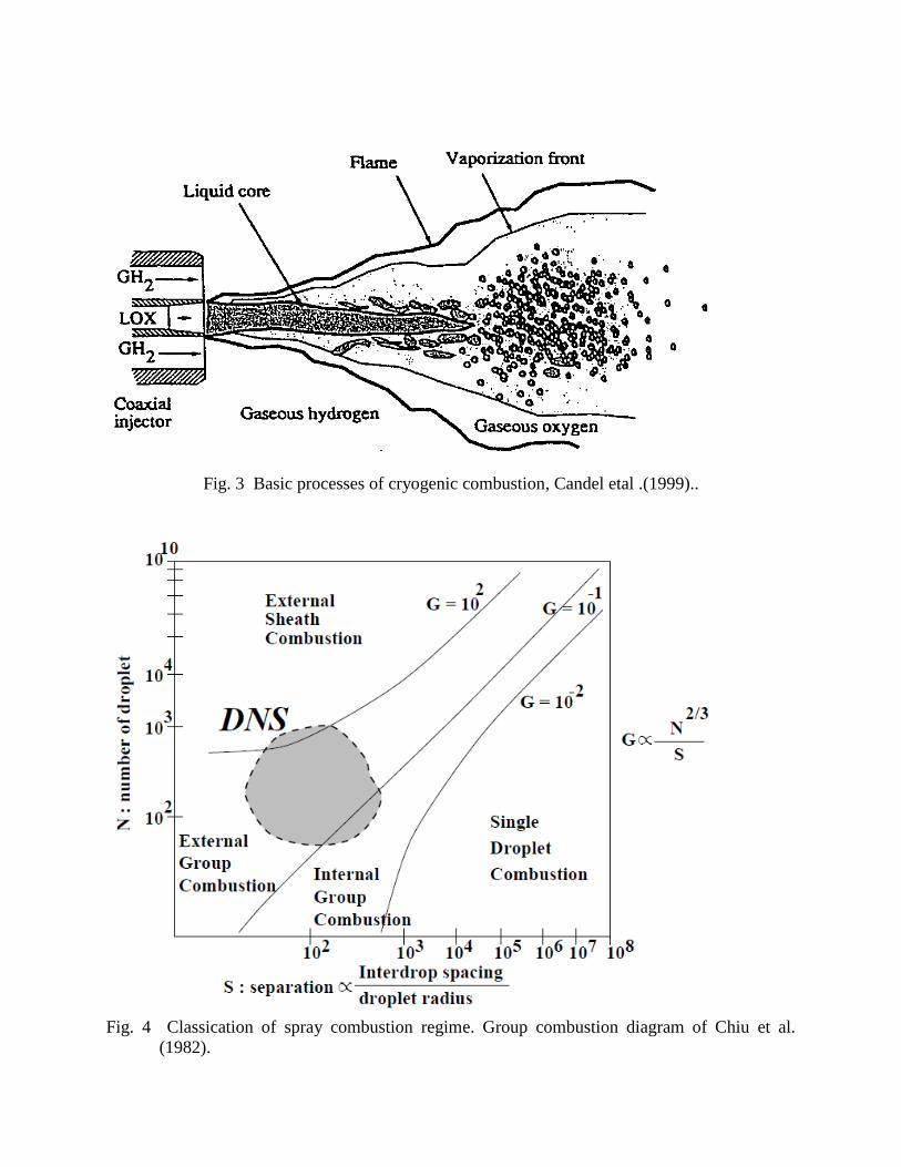
Fig. 3 Basic processes of cryogenic combustion, Candel etal .(1999)..
Fig. 4 Classication of spray combustion regime. Group combustion diagram of Chiu et al.
(1982).
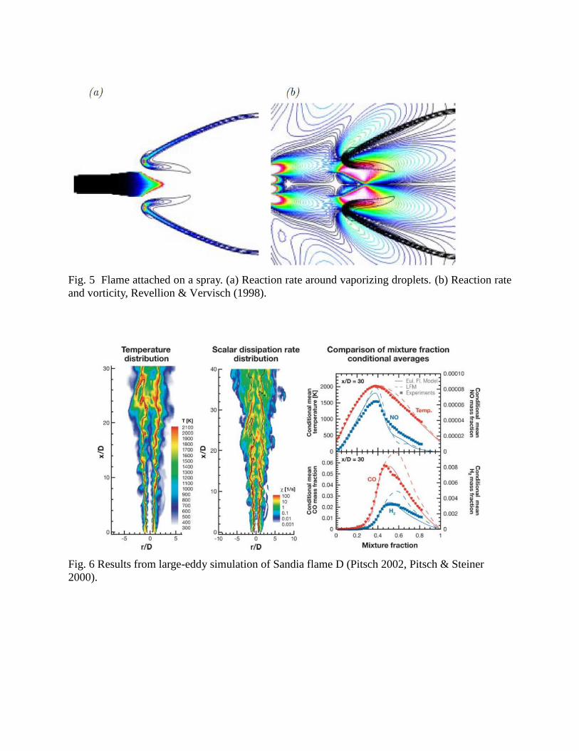
Fig. 5 Flame attached on a spray. (a) Reaction rate around vaporizing droplets. (b) Reaction rate
and vorticity, Revellion & Vervisch (1998).
Fig. 6 Results from large-eddy simulation of Sandia flame D (Pitsch 2002, Pitsch & Steiner
2000).

Fig. 7 Instantaneous and time-averaged flow properties
(Erickson, R.R., and Soteriou M.C., 2011).

Fig. 8 The steady separated flow past a circular cylinder (Grove etal., 1964).

(a)
(b)
Fig. 9 The effect of Reynolds number on the position of the vortex centre.
Re
xvc/rc
101
102
103
104
105
1060
1
2
3
4
Re
yvc/rc
101
102
103
104
105
1060
1
2
3
4

Fig. 10 Streamlines over a circular cylinder.
-0.0010 00.01
0.01
0.01
0.1
0.1
1 1
35
7
X
R
-2 -1 0 1 2 3 40
1
2
Re=50
-0.01-0.0010
00.01
0.010.1
0.11
1
3
57
X
R
-2 -1 0 1 2 3 40
1
2
Re=100
-0.010 -0.010.01
0
-0.001
0.1
-0.1
1 1
35
7
X
R
-2 -1 0 1 2 30
1
2
Re=200
-0.010 -0.010.01
-0.001
-0.001
0.1
-0.1
1 1
35
7
X
R
-2 -1 0 1 2 3 40
1
2
Re=300
-0.010 -0.10.01
-0.001
-0.001
0.1
-0.1
1 1
35
7
XR
-2 -1 0 1 2 3 40
1
2
Re=400
-0.010 -0.10.01
-0.01
-0.001
0.1
-0.1
1 1
35
7
X
R
-2 -1 0 1 2 3 40
1
2
Re=500
-0.010 -0.10.01
-0.01
-0.001
0.1
-0.1
1 1
35
7
X
R
-2 -1 0 1 2 3 40
1
2
Re=600
-0.01
-0.001
-0.001
-0.001
0
0
00.01
0.01
0.010.1
0.11 1
3
5
7
X
R
-2 -1 0 1 2 30
1
2
Re=150

Fig. 11 Schematic ‘threading diagram’ of vortex sheet in a KArmBn vortex street.
(Perry etal, 1982)
Fig. 12 Classical Vortex Shedding Alternately shed opposite signed vortices (Techet, 2004).

Fig. 13 Force time trace during the vortex shedding (Techet, 2004).
Fig. 14 Drag coefficient of a circular cylinder.
Re10
110
210
310
410
510
610-2
10-1
100
101
CD

Fig. 15 Influence of end conditions on velocity spectra in the shear layer.
(Prasad and Williamson, 1997)

Fig. 16 Comparison of s velocity spectra at Re = 2700 (Prasad and Williamson, 1997).

Fig. 17 Spectra of velocity fluctuation behind the circular cylinder.
Fig. 17 Spectra of velocity fluctuation behind the circular cylinder (Bearman, 1969)

Fig. 18 Strouhal vs. Reynolds number for the oscillatory flow cases (Yu and Jaworski).
Fig. 19 Vortex Induced Forces (Techet, 2004).
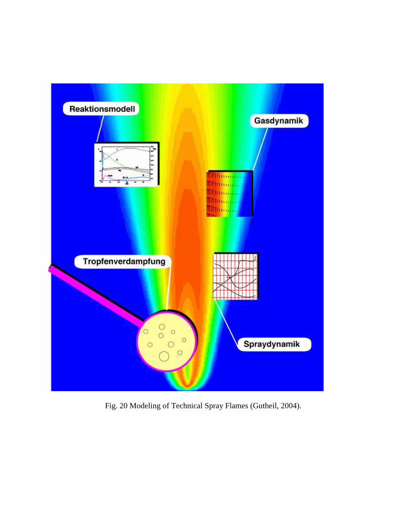
Fig. 20 Modeling of Technical Spray Flames (Gutheil, 2004).

n-Heptane/Air Spray Flame at Atmospheric Pressure
a = 500/s Detailed Chemistry: Solid Lines, Square
One-Step Chemistry: Dashed Lines, Triangles
Fig. 21 Detailed Versus One-Step Chemistry (Gutheil, 2004).

Fig. 22 H2/Air Spray Flame at Atmospheric Pressure (Gutheil, 2004).

Bidisperse monodisperse
Fig. 23 LOX/H2 Spray Flame(a) (Gutheil, 2004).
Bidisperse monodisperse
Fig. 24 LOX/H2 Spray Flame (b) (Gutheil, 2004).

.
Fig. 25 LOX/H2 Spray Flame; Chemical Reaction Rate and Vaporization Rate (Gutheil, 2004).
Fig. 26 Modeling of Turbulent Spray Flames (Gutheil, 2004).