Embed Size (px)
Citation preview

Advances in magnetic resonance imagingusing statistical signal processing
Kelvin Layton
Submitted in total fulfilment of the requirements of the degree of
Doctor of Philosophy
Department of Electrical & Electronic EngineeringTHE UNIVERSITY OF MELBOURNE
Produced on archival quality paper
May, 2013


Abstract
OVER the last 30 years, magnetic resonance imaging (MRI) has revolutioniseddiagnostic radiology by producing anatomical images of remarkable qual-
ity. MRI is often considered the most flexible imaging technique compared to otherimaging modalities and as such, the technology has helped answer fundamentalquestions about the structure and function of the body. Despite these advances,the core technology was developed at time when computer performance was lim-ited, necessitating signal approximations and clever acquisition strategies. Thedramatic increase in computer power available today means the full flexibility ofMRI can be explored.
This thesis adopts a statistical signal processing framework. From this perspec-tive, accurate models of the underlying signal and noise processes are crucial toextract the maximum information available in the measurements. This frameworkis applied to the advancement of two emerging MRI technologies: quantitativeMRI and nonlinear spatial encoding.
Quantitative MRI aims to estimate the underlying parameters contributing toa magnetic resonance signal. Unlike traditional imaging, based on contrast alone,the estimation of physical parameters promises to enhance tissue classification,disease detection and pathology. The present work examines the estimation oftransverse relaxation rates for two cases. Firstly, estimation in the presence ofdistortion due to finite sampling bandwidth is considered. Secondly, estimationof distributions of relaxation rates are considered to model voxels with multiplecomponents. Bayesian techniques are developed that incorporate accurate signalmodels and result in state-of-the-art performance.
The recent advent of nonlinear encoding fields is testament to the flexibilityinherent in MRI. These magnetic encoding fields vary nonlinearly over the field-of-view resulting in an image with spatially varying resolution. A new acquisitionstrategy that exploits this property is developed to produce images with improvedresolution in a user-specified region of interest. This technique has many applica-tions; for example, clinicians could acquire an image with high resolution detailof a brain tumour, beyond that achievable with traditional techniques. The use ofnonlinear fields creates an additional spatial dependence on the image signal-to-noise ratio and a computationally efficient metric is derived to quantity this effect.Such performance metrics are required to design new acquisition schemes thattake advantage of all possible degrees of freedom.
i


Declaration
This is to certify that
1. the thesis comprises only my original work towards the PhD,
2. due acknowledgement has been made in the text to all other material used,
3. the thesis is fewer than 100,000 words in length, exclusive of tables, maps,bibliographies and appendices.
Kelvin Layton
Date
iii

Publications
The work presented in this thesis has produced the following publications andconference presentations.
Journal papers
• Layton, K. J., Morelande, M., Wright, D., Farrell, P. M., Moran, B. and John-son, L. A. “Modelling and estimation of multi-component T2 distributions,”IEEE Transactions on Medical Imaging, 2012, (In press)
• Layton, K. J., Gallichan, D., Testud, F., Cocosco, C. A., Welz, A. M., Barmet, C.,Pruessmann, K. P., Hennig, J. and Zaitsev, M. “Single shot trajectory designfor region-specific imaging using linear and nonlinear magnetic encodingfields,” Magnetic Resonance in Medicine, 2012, (Early view)
• Layton, K. J., Morelande, M., Farrell, P. M., Moran, B. and Johnson, L. A. “Per-formance analysis for magnetic resonance imaging with nonlinear encodingfields,” IEEE Transactions on Medical Imaging, 2012, 31(2), p. 391–404
Refereed conference papers
• Layton, K. J., Morelande, M., Johnson, L. A., Farrell, P. M. and Moran, B. “Im-proved quantification of MRI relaxation rates using Bayesian estimation,”Proceedings of the IEEE Conference on Acoustics, Speech, and Signal Processing,2010, p. 481–484
• Layton, K. J., Johnson, L. A., Farrell, P. M., Moran, B. and Morelande, M.“Estimation of relaxation time distributions in magnetic resonance imaging,”Proceedings of the IEEE Conference on Acoustics, Speech, and Signal Processing,2012, p. 697–700
• Layton, K. J., Morelande, M., Farrell, P. M., Moran, B. and Johnson, L. A.“Adapting magnetic resonance imaging performance using nonlinear encod-ing fields,” Proceedings of the 33rd IEEE Engineering in Medicine and BiologyConference (EMBC), 2011, p. 3740–3743
v
Conference presentations
• Layton, K. J., Morelande, M., Farrell, P. M., Moran, B. and Johnson, L. A. “Animproved algorithm for the estimation of multi-component T2 distributions,”Proceedings of the ISMRM 20th Scientific Meeting and Exhibition, 2012
• Layton, K. J., Gallichan, D., Testud, F., Cocosco, C. A., Welz, A. M., Barmet, C.,Pruessmann, K. P., Hennig, J. and Zaitsev, M. “Region-specific trajectory de-sign for single-shot imaging using linear and nonlinear magnetic encodingfields,” Proceedings of the ISMRM 20th Scientific Meeting and Exhibition, 2012
• Layton, K. J., Morelande, M., Farrell, P. M., Moran, B. and Johnson, L. A. “Aperformance measure for MRI with nonlinear encoding fields,” Proceedingsof the ISMRM 19th Annual Meeting, 2011
• Layton, K. J., Morelande, M., Farrell, P. M., Moran, B. and Johnson, L. A.“Magnetic Resonance Imaging Using Nonlinear Encoding Fields,” The 4thAustralian Workshop on Mathematical and Computational Neuroscience, 2010
• Layton, K. J., Morelande, M., Farrell, P. M., Moran, B. and Johnson, L. A.“Quantum Mechanical Model for Magnetic Resonance Imaging,” The 3rdAustralian Workshop on Mathematical and Computational Neuroscience, 2008
vi

Acknowledgements
I would like to express my gratitude to the people who made this thesis possible.Firstly, I owe many thanks to my supervisors: Mark Morelande, Bill Moran,
Peter Farrell and Leigh Johnson for their endless patience, support and knowledge.Meetings with four enthusiastic supervisors made for many lively and enjoyablediscussions.
I am very grateful for my friends and colleagues at the Department of Electri-cal and Electronic Engineering, the Florey Neuroscience Institutes and the Centrefor Neural Engineering at The University of Melbourne: Michelle Chong, TomClose, Michael Eager, Dean Freestone, Matthieu Gilson, Colin Hales, Amir Jafar-ian, Tania Kameneva, Rob Kerr, Sei Zhen Khong, Isabell Kiral-Kornek, StephanLau, Amanda Ng, Emily O’Brien, Elma O’Sullivan-Greene, Andre Peterson, Mar-tin Spencer, Craig Savage, Evgeni Sergeev, Kyle Slater, Bahman Tahayori, AndreaVarsavsky and David Wright.
Thank you to NICTA for financial support and in particular Natasha Baxter,Domenic Santilli-Centofanti and Tracy Painter for help with conference travel andadministration matters.
I was fortunate to spend two months with the MRI group in Freiburg, whereI learnt a great deal. Thanks to Jürgen Hennig, Sebastian Littin, Hans Weber,Chris Cocosco, Cris Lovell-Smith and Benjamin Zahneisen. I’d especially like tothank Maxim Zaitsev for supervising me during my visit; and Frederik Testudand Daniel Gallichan for considerable and continued help with the nonlinear en-coding work. Thank you to Julian Maclaren and Anna Welz for the loan of theirbikes, which provided me many wonderful memories.
I am also greatly indebted to my friends. Members of Curtain Haus: MitchellLawrence, Bede Moore and Jill Pope for creating a wonderful retreat, particularlyafter days of little progress; Mark Ryan for his confidence and encouragement;Adam Baker for his grammatical and flair; the ‘Fantastic Four’; and members ofmy social sporting teams, The Outsiders, Vege Bacon Burgers and UN United forproviding a welcome distraction and much needed exercise.
I thank my loving parents, Rob and Karen, for the sacrifices they made to giveme a sound educational start and for instilling a self-belief, without which, thisthesis would never have begun. I am thankful for my sisters, Janey, Angie andTiarni for their encouragement and perspective.
Finally, I am eternally grateful to my girlfriend, Nikki, whose unwavering loveand support guided me through this often challenging time.
vii


Contents
1 Introduction 111.1 Introduction to MRI . . . . . . . . . . . . . . . . . . . . . . . . . . . . . 111.2 Motivation . . . . . . . . . . . . . . . . . . . . . . . . . . . . . . . . . . 221.3 Overview of thesis . . . . . . . . . . . . . . . . . . . . . . . . . . . . . 22
I Background 55
2 Physics of magnetic resonance 772.1 Introduction . . . . . . . . . . . . . . . . . . . . . . . . . . . . . . . . . 77
2.1.1 Notation . . . . . . . . . . . . . . . . . . . . . . . . . . . . . . . 882.2 Atomic nuclei and spin . . . . . . . . . . . . . . . . . . . . . . . . . . . 882.3 Spin dynamics . . . . . . . . . . . . . . . . . . . . . . . . . . . . . . . . 99
2.3.1 Classical description . . . . . . . . . . . . . . . . . . . . . . . . 992.3.2 Quantum description . . . . . . . . . . . . . . . . . . . . . . . 1010
2.4 Thermal equilibrium . . . . . . . . . . . . . . . . . . . . . . . . . . . . 14142.4.1 Semi-classical description . . . . . . . . . . . . . . . . . . . . . 15152.4.2 Quantum description . . . . . . . . . . . . . . . . . . . . . . . 1616
2.5 Free precession . . . . . . . . . . . . . . . . . . . . . . . . . . . . . . . 16162.5.1 Classical description . . . . . . . . . . . . . . . . . . . . . . . . 17172.5.2 Quantum description . . . . . . . . . . . . . . . . . . . . . . . 1818
2.6 RF pulse . . . . . . . . . . . . . . . . . . . . . . . . . . . . . . . . . . . 19192.6.1 Classical description . . . . . . . . . . . . . . . . . . . . . . . . 19192.6.2 Quantum description . . . . . . . . . . . . . . . . . . . . . . . 2020
2.7 Relaxation . . . . . . . . . . . . . . . . . . . . . . . . . . . . . . . . . . 21212.7.1 Classical description . . . . . . . . . . . . . . . . . . . . . . . . 21212.7.2 Quantum description . . . . . . . . . . . . . . . . . . . . . . . 2424
2.8 Summary . . . . . . . . . . . . . . . . . . . . . . . . . . . . . . . . . . . 3131
3 Principles of magnetic resonance imaging 33333.1 Introduction . . . . . . . . . . . . . . . . . . . . . . . . . . . . . . . . . 3434
3.1.1 Notation . . . . . . . . . . . . . . . . . . . . . . . . . . . . . . . 35353.2 Signal detection . . . . . . . . . . . . . . . . . . . . . . . . . . . . . . . 35353.3 Signal echoes . . . . . . . . . . . . . . . . . . . . . . . . . . . . . . . . . 3838
3.3.1 Spin echoes and CPMG echoes . . . . . . . . . . . . . . . . . . 38383.3.2 Gradient echoes . . . . . . . . . . . . . . . . . . . . . . . . . . . 4040
3.4 Spatial encoding . . . . . . . . . . . . . . . . . . . . . . . . . . . . . . . 41413.4.1 Slice selection . . . . . . . . . . . . . . . . . . . . . . . . . . . . 42423.4.2 Frequency encoding . . . . . . . . . . . . . . . . . . . . . . . . 43433.4.3 Phase encoding . . . . . . . . . . . . . . . . . . . . . . . . . . . 44443.4.4 k-space . . . . . . . . . . . . . . . . . . . . . . . . . . . . . . . . 4444
3.5 Basic sequences . . . . . . . . . . . . . . . . . . . . . . . . . . . . . . . 4545
ix

3.5.1 Cartesian . . . . . . . . . . . . . . . . . . . . . . . . . . . . . . . 45453.5.2 Radial . . . . . . . . . . . . . . . . . . . . . . . . . . . . . . . . 47473.5.3 EPI . . . . . . . . . . . . . . . . . . . . . . . . . . . . . . . . . . 4949
3.6 Image reconstruction . . . . . . . . . . . . . . . . . . . . . . . . . . . . 50503.6.1 Direct Fourier . . . . . . . . . . . . . . . . . . . . . . . . . . . . 50503.6.2 Gridding . . . . . . . . . . . . . . . . . . . . . . . . . . . . . . . 51513.6.3 Iterative . . . . . . . . . . . . . . . . . . . . . . . . . . . . . . . 5252
3.7 Properties of MRI signals . . . . . . . . . . . . . . . . . . . . . . . . . . 53533.7.1 Signal-to-noise ratio . . . . . . . . . . . . . . . . . . . . . . . . 53533.7.2 Signal processing challenges . . . . . . . . . . . . . . . . . . . 5555
II Quantitative MRI 5757
4 Estimation of relaxation rates in the presence of image distortion 59594.1 Introduction . . . . . . . . . . . . . . . . . . . . . . . . . . . . . . . . . 5959
4.1.1 Notation . . . . . . . . . . . . . . . . . . . . . . . . . . . . . . . 60604.2 Image distortion due to relaxation . . . . . . . . . . . . . . . . . . . . 6161
4.2.1 Spatial filter interpretation . . . . . . . . . . . . . . . . . . . . . 62624.2.2 Filter kernel approximation . . . . . . . . . . . . . . . . . . . . 6666
4.3 Measurement model for relaxation time estimation . . . . . . . . . . . 66664.4 Existing estimation method . . . . . . . . . . . . . . . . . . . . . . . . 6969
4.4.1 Analysis of estimation bias . . . . . . . . . . . . . . . . . . . . 70704.5 Proposed estimation method . . . . . . . . . . . . . . . . . . . . . . . 7171
4.5.1 Algorithm . . . . . . . . . . . . . . . . . . . . . . . . . . . . . . 72724.5.2 Properties of the Bayesian estimation algorithm . . . . . . . . 7373
4.6 Simulations . . . . . . . . . . . . . . . . . . . . . . . . . . . . . . . . . 74744.7 Discussion and conclusion . . . . . . . . . . . . . . . . . . . . . . . . . 7575Appendices . . . . . . . . . . . . . . . . . . . . . . . . . . . . . . . . . . . . 77774.A Introduction to the Dirichlet kernel . . . . . . . . . . . . . . . . . . . . 77774.B Closed form expression for filter kernel . . . . . . . . . . . . . . . . . 78784.C Analysis of estimation bias . . . . . . . . . . . . . . . . . . . . . . . . . 8181
5 Estimation of multi-component relaxation rate distributions 85855.1 Introduction . . . . . . . . . . . . . . . . . . . . . . . . . . . . . . . . . 8585
5.1.1 Notation . . . . . . . . . . . . . . . . . . . . . . . . . . . . . . . 87875.2 Theory . . . . . . . . . . . . . . . . . . . . . . . . . . . . . . . . . . . . 87875.3 Existing approaches . . . . . . . . . . . . . . . . . . . . . . . . . . . . . 9090
5.3.1 Pseudo-continuous model . . . . . . . . . . . . . . . . . . . . . 90905.3.2 Discrete model with unknown locations . . . . . . . . . . . . . 9191
5.4 A novel parametric and continuous model . . . . . . . . . . . . . . . 93935.5 Estimation of continuous distributions . . . . . . . . . . . . . . . . . . 9494
5.5.1 CRLB analysis . . . . . . . . . . . . . . . . . . . . . . . . . . . . 94945.5.2 NNLS and distribution width . . . . . . . . . . . . . . . . . . . 9696
5.6 Proposed estimation algorithm for the discrete model . . . . . . . . . 98985.6.1 Demonstration of algorithm . . . . . . . . . . . . . . . . . . . . 101101
x

5.6.2 Simulations . . . . . . . . . . . . . . . . . . . . . . . . . . . . . 1021025.6.3 Optic nerve experiments . . . . . . . . . . . . . . . . . . . . . . 1051055.6.4 Mouse brain experiments . . . . . . . . . . . . . . . . . . . . . 1071075.6.5 Model selection . . . . . . . . . . . . . . . . . . . . . . . . . . . 111111
5.7 Optimal experiment design . . . . . . . . . . . . . . . . . . . . . . . . 1121125.8 Discussion and conclusion . . . . . . . . . . . . . . . . . . . . . . . . . 115115Appendices . . . . . . . . . . . . . . . . . . . . . . . . . . . . . . . . . . . . 1171175.A Signal model for inverse-gamma mixture . . . . . . . . . . . . . . . . 1171175.B The extended phase graph algorithm . . . . . . . . . . . . . . . . . . . 1171175.C Partial derivatives . . . . . . . . . . . . . . . . . . . . . . . . . . . . . . 120120
III Nonlinear Spatial Encoding 123123
6 Region-specific trajectory design using nonlinear encoding fields 1251256.1 Introduction . . . . . . . . . . . . . . . . . . . . . . . . . . . . . . . . . 125125
6.1.1 Notation . . . . . . . . . . . . . . . . . . . . . . . . . . . . . . . 1271276.2 Theory . . . . . . . . . . . . . . . . . . . . . . . . . . . . . . . . . . . . 127127
6.2.1 Local k-space . . . . . . . . . . . . . . . . . . . . . . . . . . . . 1291296.3 Existing nonlinear encoding techniques . . . . . . . . . . . . . . . . . 130130
6.3.1 Cartesian PatLoc . . . . . . . . . . . . . . . . . . . . . . . . . . 1311316.3.2 O-Space . . . . . . . . . . . . . . . . . . . . . . . . . . . . . . . 1331336.3.3 4D-RIO . . . . . . . . . . . . . . . . . . . . . . . . . . . . . . . . 134134
6.4 Region specific trajectory design . . . . . . . . . . . . . . . . . . . . . 1341346.4.1 Trajectory optimisation . . . . . . . . . . . . . . . . . . . . . . 1351356.4.2 Encoding fields and target regions . . . . . . . . . . . . . . . . 1391396.4.3 Simulations . . . . . . . . . . . . . . . . . . . . . . . . . . . . . 1421426.4.4 Experiments . . . . . . . . . . . . . . . . . . . . . . . . . . . . . 1431436.4.5 Calibration . . . . . . . . . . . . . . . . . . . . . . . . . . . . . . 1441446.4.6 Safety considerations . . . . . . . . . . . . . . . . . . . . . . . . 146146
6.5 Results . . . . . . . . . . . . . . . . . . . . . . . . . . . . . . . . . . . . 1461466.5.1 Trajectory optimisation and simulations . . . . . . . . . . . . . 1461466.5.2 Experiments . . . . . . . . . . . . . . . . . . . . . . . . . . . . . 150150
6.6 Discussion . . . . . . . . . . . . . . . . . . . . . . . . . . . . . . . . . . 1521526.7 Conclusion . . . . . . . . . . . . . . . . . . . . . . . . . . . . . . . . . . 156156
7 Noise performance for imaging with nonlinear encoding fields 1591597.1 Introduction . . . . . . . . . . . . . . . . . . . . . . . . . . . . . . . . . 159159
7.1.1 Notation . . . . . . . . . . . . . . . . . . . . . . . . . . . . . . . 1611617.2 Image reconstruction using frame theory . . . . . . . . . . . . . . . . 162162
7.2.1 Review of frame theory . . . . . . . . . . . . . . . . . . . . . . 1621627.3 Analysis of block-structured encoding schemes . . . . . . . . . . . . . 166166
7.3.1 Reconstruction variance . . . . . . . . . . . . . . . . . . . . . . 1661667.3.2 SENSE imaging . . . . . . . . . . . . . . . . . . . . . . . . . . . 1681687.3.3 PatLoc imaging . . . . . . . . . . . . . . . . . . . . . . . . . . . 172172
7.4 Analysis of arbitrary encoding schemes . . . . . . . . . . . . . . . . . 178178
xi

7.4.1 Approximate reconstruction variance . . . . . . . . . . . . . . 1791797.4.2 O-Space imaging . . . . . . . . . . . . . . . . . . . . . . . . . . 180180
7.5 Simulations . . . . . . . . . . . . . . . . . . . . . . . . . . . . . . . . . 1821827.5.1 Methods . . . . . . . . . . . . . . . . . . . . . . . . . . . . . . . 1821827.5.2 Results . . . . . . . . . . . . . . . . . . . . . . . . . . . . . . . . 184184
7.6 Discussion . . . . . . . . . . . . . . . . . . . . . . . . . . . . . . . . . . 1871877.7 Conclusion . . . . . . . . . . . . . . . . . . . . . . . . . . . . . . . . . . 190190Appendices . . . . . . . . . . . . . . . . . . . . . . . . . . . . . . . . . . . . 1911917.A Basis selection . . . . . . . . . . . . . . . . . . . . . . . . . . . . . . . . 191191
8 Conclusion 1951958.1 Summary of original contributions . . . . . . . . . . . . . . . . . . . . 1951958.2 Future work . . . . . . . . . . . . . . . . . . . . . . . . . . . . . . . . . 197197
8.2.1 Statistical estimation . . . . . . . . . . . . . . . . . . . . . . . . 1971978.2.2 Nonlinear encoding . . . . . . . . . . . . . . . . . . . . . . . . 1981988.2.3 Signal modelling . . . . . . . . . . . . . . . . . . . . . . . . . . 199199
Bibliography 201201
xii

List of Figures
1.1 Schematic of an MRI scanner . . . . . . . . . . . . . . . . . . . . . . . 111.2 Overview of MRI processes and thesis contributions . . . . . . . . . . 33
2.1 Energy levels of a spin-1/2 system in a magnetic field . . . . . . . . . 14142.2 Relaxation in the laboratory frame of reference . . . . . . . . . . . . . 2222
3.1 System overview of an MRI scanner . . . . . . . . . . . . . . . . . . . 34343.2 Formation of a spin echo . . . . . . . . . . . . . . . . . . . . . . . . . . 39393.3 Timing of an RF pulse to generate a spin echo . . . . . . . . . . . . . . 39393.4 CPMG echo generation . . . . . . . . . . . . . . . . . . . . . . . . . . . 40403.5 Timing of gradients to generate a gradient echo . . . . . . . . . . . . . 41413.6 Linear spatial encoding gradients for the three imaging dimensions . 42423.7 Slice selection . . . . . . . . . . . . . . . . . . . . . . . . . . . . . . . . 43433.8 k-space sampling for a Cartesian trajectory . . . . . . . . . . . . . . . 46463.9 Sequence diagram for a Cartesian spin echo trajectory . . . . . . . . . 46463.10 k-space sampling for a radial trajectory . . . . . . . . . . . . . . . . . . 48483.11 Sequence diagram for a radial spin echo trajectory . . . . . . . . . . . 48483.12 k-space sampling for a Cartesian trajectory . . . . . . . . . . . . . . . 49493.13 Sequence diagram for a Cartesian EPI trajectory . . . . . . . . . . . . 5050
4.1 Signal amplitude during data acquisition . . . . . . . . . . . . . . . . 62624.4 Reconstructed images from simulated data using the linear filter
model . . . . . . . . . . . . . . . . . . . . . . . . . . . . . . . . . . . . . 65654.5 Reconstruction MSE for different acquisition times . . . . . . . . . . . 65654.6 Signal amplitude during a spin echo acquisition . . . . . . . . . . . . 68684.7 Magnitude slice through the centre of a two dimensional kernel . . . 69694.8 Theoretical analysis of estimation bias . . . . . . . . . . . . . . . . . . 70704.9 Estimation bias for different acquisition times and effective relax-
ation times . . . . . . . . . . . . . . . . . . . . . . . . . . . . . . . . . . 71714.10 Mean square error for the traditional and proposed estimation algo-
rithms . . . . . . . . . . . . . . . . . . . . . . . . . . . . . . . . . . . . . 74744.11 Mean square error, as acquisition time increases . . . . . . . . . . . . 75754.12 Bias and variance, as acquisition time increases . . . . . . . . . . . . . 76764.13 Dirichlet kernel dependence on the number of measurements . . . . 7777
5.1 Examples of inverse-gamma distributions . . . . . . . . . . . . . . . . 9494
xiii

5.2 Estimation bounds for multi-component parametric distributions . . 96965.3 Distribution width estimation using NNLS . . . . . . . . . . . . . . . 97975.4 Signal from a two component distribution with different widths . . . 98985.5 Demonstration of progressive correction . . . . . . . . . . . . . . . . . 1021025.6 Error in location estimates for different algorithms . . . . . . . . . . . 1041045.7 Error in flip angle estimates for different algorithms . . . . . . . . . . 1041045.8 Experimental and estimated B1 maps . . . . . . . . . . . . . . . . . . . 1061065.9 Single component T2 maps using the Bayesian algorithm . . . . . . . 1061065.10 Multi-component T2 maps using the Bayesian algorithm . . . . . . . 1081085.11 Demonstration of outliers from a gradient-based MLE algorithm . . 1091095.12 Multi-component T2 maps of a mouse brain . . . . . . . . . . . . . . . 1101105.13 Model selection criteria for an optic nerve sample . . . . . . . . . . . 1121125.14 CRLB as a function of the number of echoes . . . . . . . . . . . . . . . 1131135.15 Optimal echo spacing using the CRLB . . . . . . . . . . . . . . . . . . 1141145.16 Diagram of the extended phase graph (EPG) algorithm . . . . . . . . 118118
6.1 Example field shapes used for nonlinear spatial encoding . . . . . . . 1301306.2 Example reconstruction of a Cartesian PatLoc scheme . . . . . . . . . 1321326.3 Waveform vectors used for trajectory design . . . . . . . . . . . . . . 1391396.4 Region of interest for the optimisation schemes . . . . . . . . . . . . . 1401406.5 Gradient waveforms resulting from the optimisation procedure . . . 1471476.6 Simulation results for the optimised encoding schemes . . . . . . . . 1481486.7 Two effective encoding fields for the optimised trajectory . . . . . . . 1501506.8 Reconstruction of a phantom experiment using optimised encoding . 1511516.9 Reconstruction of an in-vivo experiment using optimised encoding . 1531536.10 Comparison of the nominal and measured trajectories . . . . . . . . . 154154
7.1 Block diagonal structure of the frame matrix for SENSE . . . . . . . . 1721727.2 Numerical phantom used for simulation . . . . . . . . . . . . . . . . . 1841847.3 Reconstruction variance of a low resolution O-Space scheme . . . . . 1851857.4 Line profiles of reconstruction variance . . . . . . . . . . . . . . . . . 1851857.5 High resolution performance map for PatLoc and O-space imaging
schemes . . . . . . . . . . . . . . . . . . . . . . . . . . . . . . . . . . . 1861867.6 Reconstruction examples for O-Space and Cartesian PatLoc schemes 188188
xiv

CHAPTER 1
Introduction
1.1 Introduction to MRI
MAGNETIC resonance imaging (MRI) has become an indispensable tool forboth clinical use and fundamental research. The utility of MRI is due to a
combination of factors. Firstly, MRI provides good contrast between different softtissues, which makes it an ideal modality for imaging the human body. Secondly,it is very safe due to the use of non-ionizing radio frequency fields. Other ma-jor imaging modalities such as nuclear medicine and X-ray use ionizing radiation,which can be harmful if exposure is not limited. Another advantage of MRI lies inits flexibility. Techniques such as structural imaging, quantitative MRI, functionalMRI, diffusion weighted imaging and MR angiography all provide complemen-tary information about the structure and function of the body.
The major drawback of MRI is cost. Machines cost millions of dollars to pur-chase and maintain. Figure 1.11.1 illustrates the costly components of an MRI scanner.A large portion of the cost is due the superconducting magnetic that generates themain magnetic field. Adding other components such gradient fields, shim coils,and radio frequency systems, the cost increases further.
A further limitation of MRI is acquisition time. Depending on the application, a
Main magnetShim coils
Gradient coilsRF coils
Figure 1.1: Schematic of an MRI scanner illustrating the main components. Imageadapted from [11]
1

2 Chapter 1. Introduction
scan can last over an hour. This time is limited both by the hardware and physicalconstraints. The patient must lie still in a relatively confined space during theacquisition period, which can be unpleasant. Additionally, patient throughput is apriority for hospitals trying to maximise the benefit of a scanner. For these reasons,decreasing the acquisition time is a topic of ongoing research.
1.2 Motivation
The fundamentals of MRI were developed during a time when computational per-formance was often a limiting factor. Since the 1990s, a dramatic increase in com-puting power has been achieved simultaneously with a large reduction in com-puter cost. This new landscape paves the way for novel acquisition strategies andadvanced processing algorithms in the field of MRI.
An MRI machine consists of many subsystems that interact in complex ways toproduce the final output. Dependent on the application, several of these interac-tions are approximated to simplify the system description and the required com-putation. Whilst these approximations are often adequate to produce high qualityresults, there is still room for improvement. This thesis describes new MRI strate-gies with detailed physical models and advanced processing algorithms necessaryto extract the desired information.
The increased computation, requisite for improved modelling, potentially per-mits two improvements. Firstly, the performance of current systems could be im-proved with a negligible increase in cost. Secondly, and perhaps more promisingly,the same level of performance might be achieved on cheaper systems. These sys-tems could be cheaper for a number of reasons, including a reduced magnetic fieldstrength, reduced field homogeneity and/or nonlinear gradient fields. Recent ap-plications of these types of systems include portable MRI or ultra-low field MRI[22].
1.3 Overview of thesis
This thesis adopts a statistical signal processing framework. Through accuratemodels of the signal and noise processes, this framework provides tools for anal-ysis and allows the maximum amount of information to be extracted from themeasurements. The framework is applied to the emerging MRI technologies ofquantitative MRI and nonlinear spatial encoding. The contributions to these re-search areas touch on a range of subcomponents of the MRI system and applica-tions. Figure 1.21.2 displays a basic schematic for MRI highlighting the contributions

1.3. Overview of thesis 3
Acquisition Protocols
Performance Metrics
Image
Relaxation Parameters
Ch 6
MRI System
Data
Hardware and sequence
Sequence
Physics Ch 2/3
Reconstruction Ch 3
Estimation Ch 4/5
Analysis Ch 7
Hardware
Figure 1.2: Overview of MRI processes and the relevant chapters discussing eachcomponent. Chapters coloured red indicate novel contributions.
made. The thesis is divided into three parts: background, quantitative MRI andnonlinear spatial encoding. Part II contains two chapters that establish the neces-sary background for the remainder of the thesis. Chapter 22 reviews the physicsunderpinning magnetic resonance from both a classical and quantum perspective.While not a strictly novel contribution, the chapter collates numerous sources in amanner not traditionally accessible in MRI literature. Boltzmann statistics are dis-cussed as the mechanism to generate macroscopic magnetisation. The Bloch equa-tion and the Schrödinger equation are presented and are used to derive the spinevolution during precession, excitation, and relaxation. The classical and quan-tum descriptions are presented alongside each other to highlight the similaritiesand provide a deeper understanding of the relevant physics. Chapter 33 presentsthe fundamentals of MRI including signal detection, echo generation, spatial en-coding and image reconstruction. The concept of k-space is introduced and usedto describe common acquisition sequences. Finally, some of the challenges specificto MRI data are discussed from a signal processing perspective.
Part IIII of this thesis includes two novel contributions to quantitative MRI.Chapter 44 examines the problem of relaxation time estimation in the presence oflocalised spatial blurring. The blurring is due to the presence of relaxation dur-ing data acquisition, described by a linear filter as in [33, 44]. This thesis extendsthe model in [44] to include contributions from both transverse relaxation and fieldinhomogeneity. The complete model is used to derive the statistical estimationbias for commonly used estimators. To overcome the issue of bias, the estimationproblem is posed using the detailed signal model and a near optimal Bayesian es-timator is developed. Chapter 55 discusses the problem of estimating a distribution

4 Chapter 1. Introduction
of relaxation times from a single decay curve, first examined in [55]. This diffi-cult problem is analysed from a statistical viewpoint using the Cramér-Rao lowerbound [66]. In light of the analysis, a novel algorithm based on the model proposedin [77, 88] is presented to estimate the main features of the distribution.
Part IIIIII contributes to the emerging field of nonlinear spatial encoding [99, 1010,1111]. Chapter 66 develops a new acquisition strategy that improves the image resolu-tion in a region of interest. The technique uses the notion of local k-space describedin [1212] to exploit the position dependent resolution inherent in nonlinear encodingfields. Chapter 77 provides a framework for image reconstruction with generalisedspatial encoding using the theory of frames [1313]. This framework is used to anal-yse the reconstruction problem for the existing schemes of SENSE [1414], PatLoc [99]and O-Space [1111] and a practical performance metric is developed based on thevariance of the reconstructed pixels.

Part I
Background
5


CHAPTER 2
Physics of magnetic resonance
Contents2.1 Introduction . . . . . . . . . . . . . . . . . . . . . . . . . . . . . . . . . 77
2.1.1 Notation . . . . . . . . . . . . . . . . . . . . . . . . . . . . . . . 882.2 Atomic nuclei and spin . . . . . . . . . . . . . . . . . . . . . . . . . . 882.3 Spin dynamics . . . . . . . . . . . . . . . . . . . . . . . . . . . . . . . 99
2.3.1 Classical description . . . . . . . . . . . . . . . . . . . . . . . . 992.3.2 Quantum description . . . . . . . . . . . . . . . . . . . . . . . 1010
2.4 Thermal equilibrium . . . . . . . . . . . . . . . . . . . . . . . . . . . . 14142.4.1 Semi-classical description . . . . . . . . . . . . . . . . . . . . . 15152.4.2 Quantum description . . . . . . . . . . . . . . . . . . . . . . . 1616
2.5 Free precession . . . . . . . . . . . . . . . . . . . . . . . . . . . . . . . 16162.5.1 Classical description . . . . . . . . . . . . . . . . . . . . . . . . 17172.5.2 Quantum description . . . . . . . . . . . . . . . . . . . . . . . 1818
2.6 RF pulse . . . . . . . . . . . . . . . . . . . . . . . . . . . . . . . . . . . 19192.6.1 Classical description . . . . . . . . . . . . . . . . . . . . . . . . 19192.6.2 Quantum description . . . . . . . . . . . . . . . . . . . . . . . 2020
2.7 Relaxation . . . . . . . . . . . . . . . . . . . . . . . . . . . . . . . . . . 21212.7.1 Classical description . . . . . . . . . . . . . . . . . . . . . . . . 21212.7.2 Quantum description . . . . . . . . . . . . . . . . . . . . . . . 2424
2.8 Summary . . . . . . . . . . . . . . . . . . . . . . . . . . . . . . . . . . . 3131
2.1 Introduction
SPIN is the fundamental property of nuclei that makes MR imaging possible.Understanding the physics describing the behaviour of spins is essential to
accurately model the behaviour of the MR signal. Thus a detailed description ofthe physics describing systems of one or many spins is provided in this chapter.The behaviour is examined from both a classical and quantum perspective to givea deeper understanding of the topics covered. The chapter explores the basics ofspin systems with focus on spin-1/2 systems relevant to MRI. An introduction
7

8 Chapter 2. Physics of magnetic resonance
Table 2.1: Common notation used in Chapter 22
Symbol Quantity Units
Physical constantsKB Boltzmann constant, 1.3807× 10⁻²³ J K−1
h Reduced Planck’s constant, 1.0546× 10⁻³⁴ J sγ Gyromagnetic ratio, 2.6751× 10⁸ (for 1H) rad/s/T
Classical physicsb Magnetic field Tm MagnetisationT1, T2 Longitudinal and transverse relaxation times si, j, k Unit vectors along the x, y and z axesp(ω) Distribution of isochromatsλ Width of Lorentzian distribution
Quantum physicsψ(t) Quantum stateρ Density matrix|α〉, |β〉 EigenstatesH Hamiltonian operatorA Basis operators for Hamiltonian decompositionF(t) Coefficients of Hamiltonian decompositionJ(ω) Spectral density functionsIx, Iy, Iz Spin angular momentum operatorsR Rotation operatorΓ Relaxation operator
to concepts such as thermal equilibrium, precession, RF pulses and relaxation isprovided.
2.1.1 Notation
Table 2.12.1 lists the important quantities and their associated notation used in thischapter. Other notation not listed in this table will be introduced as it is required.
2.2 Atomic nuclei and spin
Matter is made up of atoms which in turn are made up of electrons and nuclei.Nuclei consists of sub-atomic particles such as quarks and gluons. Nuclei havefour physical properties that arise from the properties of these sub-atomic parti-cles: mass, electric charge, magnetic moment and spin. The magnetic moment, µ,
2.3. Spin dynamics 9
is related to the spin, S, by a fundamental symmetry theorem[1515, page 26]. That is,
µ = γS (2.1)
where γ is the gyromagnetic ratio. This means that depending on the sign of γ, thespin angular momentum is either aligned with the magnetic moment, or oppositeit. The gyromagnetic ratio is positive for most magnetic nuclei (including 1H) andnegative for electrons and a few atomic nuclei.
2.3 Spin dynamics
In this section we describe both classical and quantum descriptions of a spin sys-tem. In both cases, the dynamics of the spins is governed by a differential equation:the Bloch equation for a classical description and the Schrödinger equation (or Li-ouville equation) for quantum states.
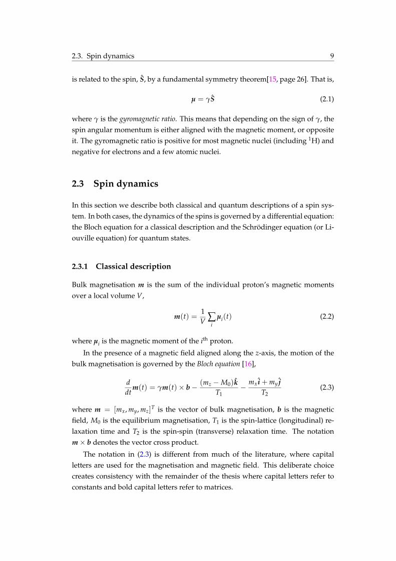
2.3.1 Classical description
Bulk magnetisation m is the sum of the individual proton’s magnetic momentsover a local volume V,
m(t) =1V ∑
iµi(t) (2.2)
where µi is the magnetic moment of the ith proton.
In the presence of a magnetic field aligned along the z-axis, the motion of thebulk magnetisation is governed by the Bloch equation [1616],
ddt
m(t) = γm(t)× b− (mz −M0)kT1
− mx i + my jT2
(2.3)
where m = [mx, my, mz]T is the vector of bulk magnetisation, b is the magneticfield, M0 is the equilibrium magnetisation, T1 is the spin-lattice (longitudinal) re-laxation time and T2 is the spin-spin (transverse) relaxation time. The notationm× b denotes the vector cross product.
The notation in (2.32.3) is different from much of the literature, where capitalletters are used for the magnetisation and magnetic field. This deliberate choicecreates consistency with the remainder of the thesis where capital letters refer toconstants and bold capital letters refer to matrices.

10 Chapter 2. Physics of magnetic resonance
2.3.1.1 Rotating Frame of Reference
A common convention in MRI is to define the main magnetic field along the z-direction such that
b = B0k (2.4)
In this case, a useful tool for analysis is to transform the Bloch equation to a rotat-ing frame of reference where the x-y plane rotates about the z axis at the Larmorfrequency ω0. The Bloch equation in the rotating frame of reference becomes
ddt
m′(t) = γm′(t)× beff −(mz′ −M0)k
′
T1− mx′ i
′+ my′ j
′
T2(2.5)
where beff = b′ + ωrot/γ is the effective field in the rotating frame. The vectorωrot describes the speed and direction of the rotating frame and b′ and m′ arethe magnetic field and magnetisation transformed to the rotating frame. By con-vention, ωrot = −ωk so the reference frame rotates in the same direction as spinprecession. Often throughout this thesis the prime notation is used to indicate therotating frame of reference. To distinguish from the rotating frame of reference, werefer to the static or non-rotating frame as the ‘laboratory’ frame of reference.
2.3.2 Quantum description
The state of a single quantum particle is described by a complex-valued wavefunc-tion, ψ(x, t). In this thesis we consider stationary particles and drop the spatialvariable, x from the notation. For a spin-1/2 particle, there are two eigenstates ofangular momentum along the z-axis called Zeeman eigenstates,
|α〉 =∣∣∣∣12,+
12
⟩; |β〉 =
∣∣∣∣12,−12
⟩(2.6)
where the notation, |I, M〉 specifies the eigenstate using two quantum numbers, Iand M. These eigenstates are useful since an arbitrary state can be described asa linear combination (or superposition) of these basic states. The state |ψ〉 can bewritten as |ψ〉 = cα|α〉+ cβ|β〉 or in vector form
|ψ〉 =[
cα
cβ
](2.7)

2.3. Spin dynamics 11
where the Zeeman eigenstates are written as
|α〉 =[
10
]; |β〉 =
[01
](2.8)
The dynamics of the spin state, |ψ〉, is given by the time-dependent Schrödingerequation. In natural units (scaled by h−1) the equation is
ddt
ψ(t) = −jH ψ(t), (2.9)
where j =√−1. This equation completely describes the evolution of the quantum
states of the particle.
A magnetic resonance experiment is only capable of observing the average ef-fect of all spins in an object. The average state of a spin ensemble is accuratelydescribed using the density matrix. Formally, the density matrix can be defined byconsidering the summation of Ns spins with states, |ψi〉, i = 1, . . . , Ns as follows[1717],
ρ =1
Ns
Ns
∑i=1|ψi〉〈ψi| (2.10)
where 〈ψi| denotes the transpose of |ψi〉. Each state, |ψi〉 can be defined as in (2.72.7)in terms of the Zeeman eigenstates, |α〉 and |β〉 denoting the low and high energystates, respectively. Using this representation, the density matrix can be written asfollows,
ρ =
[cαc∗α cαc∗βcβc∗α cβc∗β
]=
[ραα ραβ
ρβα ρββ
](2.11)
The overbar indicates an average over the ensemble. Diagonal terms (ραα andρββ) are called populations and off-diagonal terms (ραβ and ρβα) are called coherences.They have the following relationships [1717],
ραβ = ρ∗βα (2.12)
ραα + ρββ = 1 (2.13)
A physical interpretation of these quantities is useful to develop some intuition.The population difference represents the net polarisation along the external fielddirection. Thus if ραα − ρββ > 0, the net polarisation is aligned with the externalfield. The presence of non-zero coherences indicates transverse spin magnetisa-

12 Chapter 2. Physics of magnetic resonance
tion, that is a net polarisation perpendicular to the external field, B0.
The system dynamics are governed by the time-dependent Schrödinger equa-tion (2.92.9) from which the Liouville equation for the density operator is derived [1818,page 369]
ddt
ρ(t) = −j[H , ρ(t)] (2.14)
where [A, B] = AB− BA is known as the commutator. Importantly, two operatorsA and B are said to commute if and only if [A, B] = 0.
2.3.2.1 Rotating Frame of Reference
Analogous to the classical rotating frame of reference, the Schrödinger equationcan be transformed to rotating coordinate system [1919]. This reference frame is oftenreferred to as the interaction frame. The system is transformed using the operator,Rz, representing a rotation around the z-axis,
Rz(φ) =
[exp−j 1
2 φ 00 exp+j 1
2 φ
](2.15)
Using this operator, a single spin state is transformed to the rotating frame of ref-erence according to
|ψ〉(t) = Rz(ωreft)|ψ〉(t) (2.16)
where ωref is the frequency of rotation and |ψ〉(t) is the state in the rotating frameof reference. The Hamiltonian in the rotating frame is transformed according to
H = Rz(−ωreft)H Rz(ωreft)−ωref Iz (2.17)
Finally, the Schrödinger equation in the interaction frame is
ddt
ψ(t) = −jH ψ(t) (2.18)
For an ensemble of spins, the density operator in the rotating-frame, ρ, is de-fined as
ρ = |ψ〉〈ψ| (2.19)
where ψ is a single state in the rotating frame (defined in (2.162.16)) and the overbar de-notes an ensemble average. Equivalently, the density operator can be transformed

2.3. Spin dynamics 13
directly using
ρ(t) = Rz(ωreft)ρ(t)Rz(−ωreft) (2.20)
In this frame of reference the Liouville equation becomes
ddt
ρ(t) = −j[H , ρ(t)]. (2.21)
2.3.2.2 Observations
A key feature of quantum mechanics is that it only provides the probabilities ofobserving particular results. Each observation is associated with a Hermitian op-erator and the result of an experimental observation is an eigenvalue of that op-erator. Specifically, the probability of observing the eigenvalue λn for observableoperator, Q, is
Pr(λn) = |〈ξn|ψ〉|2 (2.22)
where |ξn〉 is the eigenvector associated with the eigenvalue λn. Note that if thestate is initially an eigenvector the probability of observing the correspondingeigenvalue is 1.
Although the result of a single observation is undefined prior to the actualmeasurement, the expectation is well defined as
〈Q〉 = 〈ψ|Q|ψ〉 (2.23)
= Tr|ψ〉〈ψ|Q (2.24)
where Tr denotes the matrix trace.
The motivation for using the density operator lies in its ability to describemacroscopic observations. The average outcome from measuring individual spinsof an ensemble is the sum of the expectation values.
Qobs = Tr(|ψ1〉〈ψ1|+ |ψ2〉〈ψ2|+ · · · )Q (2.25)
Substituting the density operator definition in (2.102.10) gives
Qobs = NsTrρQ (2.26)
From this viewpoint, the contribution of each spin to the macroscopic observationis TrρQ.

14 Chapter 2. Physics of magnetic resonance
B0
E
|α〉
|β〉∆E = γhB0
E = 12 γhB0
E = − 12 γhB0
Figure 2.1: The energy levels of a spin-1/2 system in a magnetic field, illustratinglow energy states, |α〉, and high energy states, |β〉. The energy difference, ∆E,between states increases linearly with field strength, B0.
The most useful measurement operators are the spin angular moment opera-tors,
Ix =12
[0 11 0
]; Iy =
12
[0 −jj 0
]; Iz =
12
[1 00 −1
]. (2.27)
The notation of macroscopic observation can be used to relate the bulk mag-netisation vector of the classical description, m = mx i + my j + mzk, to the densitymatrix using
mz = C Tr(ρ Iz)=
12
C(ραα − ρββ) (2.28a)
mx = C Tr(ρ Ix)= C Re(ρβα) (2.28b)
my = C Tr(ρ Iy)= C Im(ρβα) (2.28c)
where the constant, C, is dependent on the thermal equilibrium and the numberof spins, Ns. In Section 2.42.4 we will see how to define the constant in a meaningfulway.
2.4 Thermal equilibrium
At thermal equilibrium, in the presence of an external magnetic field in the z-direction, the spins of a spin-1/2 system are observed in one of two possible ori-entations, spin-up or spin-down.
Spins in different orientations have different energy, a phenomena known asZeeman splitting. The energy difference is ∆E = Eβ − Eα = γhB0. Figure 2.12.1 illus-trates this phenomena and demonstrates that the energy difference is proportionalto the field strength, B0. Spins parallel to the B0 field are in lower energy statethan spins anti-parallel. This creates a population difference between the two spin

2.4. Thermal equilibrium 15
states that is related to the energy difference, ∆E, according to the Boltzmann dis-tribution,
p(α) =exp(−Eα/KBT)
exp(−Eα/KBT) + exp(−Eβ/KBT)(2.29)
p(β) =exp(−Eβ/KBT)
exp(−Eα/KBT) + exp(−Eβ/KBT)(2.30)
Since ∆E KBT the exponentials can be approximated to first order by
exp(− E
KBT
)≈ 1− E
KBT(2.31)
Noting that Eα = − 12 ∆E and Eβ = + 1
2 ∆E, the probabilities can be written as
p(α) ≈ 1 + B/22
; p(β) ≈ 1−B/22
(2.32)
where B denotes the Boltzmann factor, defined as
B ,∆EKBT
=γhB0
KBT. (2.33)
As an example we consider a typical MRI situation. An object is placed in a3 T magnetic field at room temperature, T = 300 K. Substituting these values andthe known physical constants into (2.332.33) results in probabilities such that approx-imately nine in one million protons contribute to the signal. Since the number ofprotons in a typical object is many orders of magnitude greater than one million,this tiny fraction is sufficient to provide high quality magnetic resonance data.
2.4.1 Semi-classical description
Thermal equilibrium can be described from a classical perspective by consideringthe number of up spins, N↑, and the number of down spins, N↓. This is given bythe appropriate fraction of the total number of spins, Ns resulting in a populationdifference of
N↑ − N↓ = Ns (p(α)− p(β)) ≈ NsB
2(2.34)
The spin orientation of an individual proton directly defines the direction ofthe magnetic moment vector according to according to the relation in (2.12.1). Forspin-1/2 systems, the magnetic moment of the ith proton is, µi = ± 1
2 γhk, wherethe sign depends on the orientation of the proton’s spin. The bulk magnetisation
16 Chapter 2. Physics of magnetic resonance
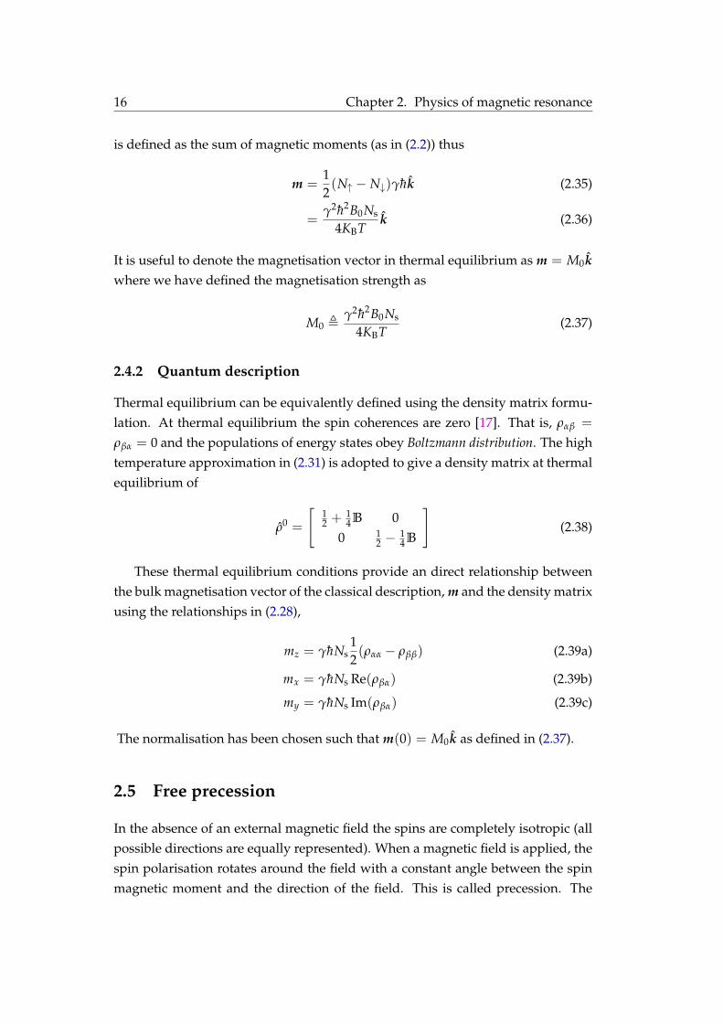
is defined as the sum of magnetic moments (as in (2.22.2)) thus
m =12(N↑ − N↓)γhk (2.35)
=γ2h2B0Ns
4KBTk (2.36)
It is useful to denote the magnetisation vector in thermal equilibrium as m = M0kwhere we have defined the magnetisation strength as
M0 ,γ2h2B0Ns
4KBT(2.37)
2.4.2 Quantum description
Thermal equilibrium can be equivalently defined using the density matrix formu-lation. At thermal equilibrium the spin coherences are zero [1717]. That is, ραβ =
ρβα = 0 and the populations of energy states obey Boltzmann distribution. The hightemperature approximation in (2.312.31) is adopted to give a density matrix at thermalequilibrium of
ρ0 =
[12 +
14 B 0
0 12 − 1
4 B
](2.38)
These thermal equilibrium conditions provide an direct relationship betweenthe bulk magnetisation vector of the classical description, m and the density matrixusing the relationships in (2.282.28),
mz = γhNs12(ραα − ρββ) (2.39a)
mx = γhNs Re(ρβα) (2.39b)
my = γhNs Im(ρβα) (2.39c)
The normalisation has been chosen such that m(0) = M0k as defined in (2.372.37).
2.5 Free precession
In the absence of an external magnetic field the spins are completely isotropic (allpossible directions are equally represented). When a magnetic field is applied, thespin polarisation rotates around the field with a constant angle between the spinmagnetic moment and the direction of the field. This is called precession. The

2.5. Free precession 17
frequency of precession is given by the Larmor frequency, ω0,
ω0 = γB0 (2.40)
where B0 is the magnetic field strength. This section examines this phenomenausing classical and quantum descriptions.
2.5.1 Classical description
The presence of a static magnetic field causes the magnetisation to rotate aroundthe direction of the field, a phenomenon known as precession. To see this, we solvethe Bloch equation for a magnetic field aligned with the z-axis, b = B0k. We ignorerelaxation effects by assuming t T1, T2, which is realistic for short timescales. Inthis case,
ddt
m(t) = γm(t)× b. (2.41)
Given an arbitrary initial condition, m0 = mx(0)i + my(0) j + mz(0)k, the solutionto (2.412.41) is
m(t) = Mxy(0) cos(ω0t + φ0)i + Mxy(0) sin(ω0t + φ0) j + Mz(0)k (2.42)
where Mxy(0) =√
m2x(0) + m2
y(0), ω0 = γB0 and φ0 = arctan(my(0)/mx(0)). Itis often instructive to consider the transverse magnetisation as a complex number,i.e.,
mxy(t) = mx(t) + jmy(t) (2.43)
With this notation the solution can be written as
mxy(t) = Mxy(0)e−j(ω0t+φ0) (2.44a)
mz(t) = Mz(0) (2.44b)
This clearly shows the bulk magnetisation precesses around the external field atthe Larmor frequency ω0 = γB0.
Alternatively, we can use (2.52.5) to describe the magnetisation in a referenceframe rotating at the Larmor frequency. We have b = B0k and ωrot = −γB0kso beff = 0. Neglecting relaxation leads to the condition,
ddt
m′(t) = 0. (2.45)

18 Chapter 2. Physics of magnetic resonance
As expected, the bulk magnetisation is stationary in the rotating frame.
2.5.2 Quantum description
The Hamiltonian in the presence of a static magnetic field B0 along the z-axis isH = ω0 Iz. The Schrödinger equation describing the state evolution is
ddt|ψ〉(t) = −jω0 Iz|ψ〉(t) (2.46)
The solution to this equation is
|ψ〉(t) = exp−jω0t Iz|ψ〉(0) (2.47)
This can be recognised as a rotation about the z-axis and hence it can be describedwith the rotation operator in (2.152.15),
|ψ〉(t) = Rz(ω0t)|ψ〉(0) (2.48)
This means that in the absence of an RF field, the Schrödinger equation impliesthat the spin rotates around the z-axis with frequency ω0.
The Liouville equation can be solved to determine the evolution of the densitymatrix under a static magnetic field. Alternatively, we can use the evolution of asingle state given in (2.482.48) to build the density matrix according to the definitionin (2.102.10). In this case,
ρ(t) = R(ω0t)ρ(0)R(−ω0t) (2.49)
Computing the individual elements of the matrix gives the following set of equa-tions
ραα(t) = ραα(0) (2.50a)
ρββ(t) = ρββ(0) (2.50b)
ραβ(t) = exp−jω0tραβ(0) (2.50c)
ρβα(t) = expjω0tρβα(0) (2.50d)
Ignoring relaxation, we see that the populations of the states remains unchangedand the coherences revolve around the complex plane at the resonant frequencyω0.

2.6. RF pulse 19
2.6 RF pulse
2.6.1 Classical description
When a rotating magnetic field B1(t) is applied perpendicular to the B0 field at theLarmor frequency of the spin system, the effect is to tilt the bulk magnetisationaway from the z-axis. To see this consider a circularly polarised field,
b1(t) = B1(t)
sin(ωrft + φp)i + cos(ωrft + φp) j
(2.51)
where B1(t) is the amplitude envelope, ωrf is the frequency of oscillation and φp isthe initial phase angle.
To analyse the effect of such a pulse, we make the reasonable assumption thatthe RF pulse is short enough such that relaxation effects can be ignored for theduration of the pulse. The rotating frame Bloch equation in (2.52.5) reduces to
∂
∂tm′(t) = γm′(t)× beff (2.52)
where beff = b′ + ωrot/γ. Further, we assume the RF pulse has zero phase andconstant envelope, B1(t) = B1, 0 ≤ t ≤ Tp, The RF pulse in (2.512.51) can be trans-formed to the rotating frame to give, b′1(t) = B1 i. When the resonance condition issatisfied (i.e. ωrf = ω0), and we adopt the Larmor rotating frame (ωrot = −ω0k),the effective magnetic field is
beff = B0k′+ B1 i′ − ω0
γk = B1 i′ (2.53)
The Bloch equation can be easily solved for an initial condition of m′(0) = M0k′
to give
m′(t) = M0sin(ω1t) j′ + cos(ω1t)k′ (2.54)
where ω1 = γB1 is known as the Rabi frequency and represents the rotation speedof the bulk magnetisation away from the z-axis. This equation determines themotion of the bulk magnetisation for the duration of the pulse. At t = Tp the bulkmagnetisation has been rotated about the x′-axis through a flip angle θ = ω1Tp.For more complex envelopes the flip angle is given by
θ =∫ Tp
0γB1(τ)dτ. (2.55)

20 Chapter 2. Physics of magnetic resonance
This equation is valid for on-resonance excitation with a duration sufficiently shortcompared to the relaxation times.
2.6.2 Quantum description
During an RF pulse the spin Hamiltonian is made up of the static HamiltonianH0 and RF Hamiltonian, Hrf(t). Ignoring any off-resonance effects, the completeHamiltonian is given in [2020] as
H (t) = H0 +Hrf (2.56)
= ω0 Iz − γB1cos(ωrft + φp) Ix + sin(ωrft + φp) Iy (2.57)
We transform the system to a reference frame rotating at ωrf about the z-axis.The transformed Hamiltonian is computed using (2.172.17). Simplifying with the“sandwich relationship”, the final Hamiltonian can be expressed as
H = ωoff Iz + ωnut(
Ix cos φp + Iy sin φp)
(2.58)
where ωoff = ω0 − ωrf and ωnut = |γB1|. Note the Hamiltonian in the rotatingframe of reference is independent of time.
When the pulse is applied exactly on resonance (ωoff = 0), the solution to theSchrödinger equation is
|ψ〉(t) = Rφp(ωnutt)|ψ〉(0). (2.59)
This can be recognised as a rotation of the initial state using the general rotationoperator, Rφp(θ) = Rz(φp)Rx(θ)Rz(−φp).
Now consider an on-resonance ‘x-pulse’, where φp = 0. The rotating-framespin Hamiltonian is H = ωnut Ix and the solution is a rotation about the x′-axis.For example, suppose the initial state is the eigenstate |α〉; after time τp = π/(2ωnut)
the spin will be rotated through a flip angle of π/2 given by the equation
|ψ〉(τp) = Rx(π/2)|α〉 (2.60)
The evolution of the density matrix can be derived by averaging the effect ofan RF pulse on individual states evolving according to (2.592.59). The evolution of thedensity operator is
ρ(t) = Rφp(ωnutt)ρ(0)Rωnutt(−ωnutt) (2.61)

2.7. Relaxation 21
After time τp the density matrix has been rotated by angle θ defined in (2.552.55). No-tice that a π pulse inverts the population distribution while a π/2 pulse equalisesthe spin state populations and generates coherences.
2.7 Relaxation
There are two types of relaxation processes in a spin system caused by differentphysical mechanisms: spin-lattice relaxation and spin-spin relaxation.
Spin-lattice relaxation refers to the process by which the spin system exchangesenergy with its external surroundings (or lattice). This is associated with transi-tions from high energy states to low energy states, which affects the populationdifference of the spin states and ultimately the longitudinal magnetisation. Thetime constant T1 is associated with the time required for the spin system to reachthermal equilibrium. For these reasons spin-lattice relaxation is also known as T1
or longitudinal relaxation.
Spin-spin relaxation, on the other hand, involves the spins exchanging energyamong themselves. For example, one spin may cause a second spin to transitionfrom high to low energy states while the first spin transitions from low to highenergy. In this case, the population of states does not change and the longitudinalmagnetisation will not be affected. However, transitions of this type result in a lossof coherence between spin states. This coherence loss manifests as a decrease intransverse magnetisation related to the time constant, T2. This type of relaxation isthus referred to as T2 or transverse relaxation.
This description illuminates the close relationship between the molecular struc-ture of an object and relaxation. Images produced by MRI machines are stronglydependent on the relaxation properties and therefore the underlying structure.The difference between relaxation properties of normal and diseased tissues is of-ten the basis for a diagnosis using MRI. Table 2.22.2 lists some typical values for T1, T2
and M0 for various healthy tissue types at 1.5 T [2121] although the values can varysignificantly depending on the particular experiment (see e.g. [2222]).
In the following section we examine these relaxation processes in more detail.This is important to gain a deeper understanding of the relaxation parameters weestimate in Chapters 44 and 55.
2.7.1 Classical description
Consider the evolution of the magnetisation after an RF pulse has been applied.The main B0 magnetic field is still present along the z-direction. The Bloch equa-

22 Chapter 2. Physics of magnetic resonance
Table 2.2: Typical values of proton density and relaxation time constants, T1 andT2 for biological tissue at 1.5 T. Sourced from [2121].
Tissue Type T1 (ms) T2 (ms) M0
CSF 2400 160 1.0White matter 780 90Gray Matter 900 100Muscle 870 45Liver 500 40Fat 270 80 0.9
0 0.5 1 1.5 2 2.5 3
−1
−0.8
−0.6
−0.4
−0.2
0
0.2
0.4
0.6
0.8
1
t (s)
Magnetisa
tion
mx(t)
m y(t)
|mx y(t)|
m z(t)
(a)
y
z
x
(b)
Figure 2.2: Relaxation viewed in the laboratory frame of reference illustrating (a)(a)the individual components of the magnetisation vector during relaxation and (b)(b)the trajectory of the tip of the magnetisation vector.
tion can be solved in the rotating frame using (2.52.5). Adopting the complex notationin (2.432.43) the solution is
mx′y′(t) = mx′y′(0)e−t/T2 (2.62a)
mz′(t) = M0(1− e−t/T1) + mz′(0)e−t/T1 (2.62b)
where mx′y′(0) and mz′(0) define the magnetisation immediately after the pulse.This solution can easily be interpreted as a decaying transverse magnetisation withtime constant T2, and a recovering longitudinal magnetisation with time constantT1. Figure 2.22.2 illustrates the evolution of the bulk magnetisation for T1 = 1 s andT2 = 500 ms. To emphasise the general behaviour, the system was simulated witha Larmor frequency many orders of magnitude below realistic values.
In addition to these two relaxation processes, spins in the object experience

2.7. Relaxation 23
different local fields due to inhomogeneity and/or applied gradients. The localfield variation leads to spins with a distribution of different precession frequencies.The term isochromat is used to define a group of spins with the same precessionfrequency. In the laboratory frame of reference, the transverse magnetisation froma single isochromat (with Larmor frequency ω) is
mxy(t, ω) = mxy(0)e−t/T2 ejωt (2.63)
The final signal observed is the integration of the relative contributions of all suchisochromats,
mxy(t) =∫
mxy(t, ω)p(ω)dω (2.64)
where p(·) is the distribution of isochromats.
Some intuition can be gained by considering a Lorentzian distribution of theLarmor frequencies,
p(ω) =1π
λ
λ2 + (ω−ω0)2 (2.65)
where ω0 is the centre of the distribution and λ is half-width at half-maximum(HWHM) representing the distribution spread. It should be noted that, despiteits prevalence, there is no physical reason to adopt a Lorentzian distribution. Itis chosen for mathematical convenience. Nonetheless, it is useful to demonstratesome general properties of the free induction decay. In this case, the integral in(2.642.64) can be calculated in closed form using the Fourier transform, F , as follows.
mxy(t) =∫
mxy(0)e−t/T2 ejωt p(ω)dω (2.66)
= mxy(0)e−t/T2
∫ejωt p(ω)dω (2.67)
= mxy(0)e−t/T2(F p)(t) (2.68)
= mxy(0)e−t/T2 e−λte−jω0t (2.69)
This highlights the effect of the distribution on transverse relaxation. Specifically,the frequency distribution adds an additional relaxation component dependent onthe spread of frequencies, λ. A very narrow distribution will result in an ideal T2
decay, while a wide distribution will result in a faster decay. This can also be un-derstood using the notion of dephasing discussed in Chapter 33. For the Lorentziandistribution, both relaxation processes can be aggregated into a single exponential

24 Chapter 2. Physics of magnetic resonance
decay,
mxy(t) = mxy(0)e−t/T∗2 e−jω0t (2.70)
where the time constant T∗2 consists of T2 and T′2 = 1/λ according to
1T∗2
=1T2
+1T′2
(2.71)
2.7.2 Quantum description
At a quantum physics level, relaxation is mostly due to the following mechanisms:1) dipole-dipole coupling, 2) chemical shift anisotropy, 3) spin-rotation interaction.The order listed is the usual order of importance where chemical shift becomesincreasingly important at high field strengths and begins to compete with dipole-dipole coupling.
2.7.2.1 Internal Spin Interactions
The spin angular momentum is affected by the magnetic and electric fields of in-teracting particles in the sample. A single proton undergoes rapid movement andelectromagnetic interactions with neighbouring particles (protons, electrons etc),each of which has its own magnetic moment. This causes tiny fluctuations in themagnetic field experienced by a given proton. The physical interaction mecha-nisms are described below:
Chemical Shift External magnetic field affects magnetism of electrons and they inturn affect the nuclear spin.
Dipole-Dipole Coupling Direct magnetic interactions of nuclear spins with eachother.
J-Coupling Indirect magnetic interactions of nuclear spins, via interactions withelectrons.
Spin-Rotation Interaction Nuclear spins interacting with magnetic fields gener-ated by the rotational motion of the molecules.
Quadrupolar Coupling (for spins > 1/2) Electric interactions of nuclei with sur-rounding electric fields.
For spin-1/2 nuclei dipole-dipole and chemical shift interactions are the strongest[1515]. All these interactions cause fluctuations in the local magnetic field and resultin the relaxation effects described below.

2.7. Relaxation 25
The appropriate Hamiltonian describing these microscopic interactions can beused to derive the evolution of the spin system towards thermal equilibrium, i.e.,relaxation.
2.7.2.2 Integral Form
The complete system Hamiltonian is composed as follows,
H (t) = H0 +H1(t) (2.72)
where H0 is the static Hamiltonian and H1 is the interaction Hamiltonian.The system dynamics are governed by Liouville equation in (2.142.14). To simplify
the calculations, we transform the system to the interaction frame using
ρ(t) = exp+jH0tρ(t) exp−jH0t (2.73)
H1(t) = exp+jH0tH1(t) exp−jH0t (2.74)
The Liouville equation for the combined system in the interaction frame is
ddt
ρ(t) = −j[H1(t), ρ(t)] (2.75)
Integrating this equation by successive approximations up to second order gives
ρ(t) ≈ ρ(0)− j∫ t
0[H1(t′), ρ(0)]dt′ −
∫ t
0dt′∫ t′
0dt′′[H1(t′), [H1(t′′), ρ(0)]] (2.76)
Differentiating (2.762.76) with respect to time gives the ‘integrated to second order’approximation [2323, page 276] and a change of variable (τ = t− t′) gives
ddt
ρ(t) ≈ −j[H1(t), ρ(0)]−∫ t
0dτ[H1(t), [H1(t− τ), ρ(0)]] (2.77)
Since H1(t) is a random operator, (2.772.77) indicates that ρ(t) is also a random opera-tor and the observable behaviour will be described by an average density operatorρ which is described by the above equation averaged over all the random Hamil-tonians H1(t). The average equation is
ddt
ρ(t) ≈ −j[H1(t), ρ(0)]−∫ t
0dτ[H1(t), [H1(t− τ), ρ(0)]] (2.78)
Now the following assumptions are made:
A2.1 H1(t) = 0. Otherwise, we can redefine H0 to include it.

26 Chapter 2. Physics of magnetic resonance
A2.2 We can neglect the correlation between H1(t) and ρ(0) and average themseparately.
A2.3 We can replace ρ(0) by ρ(t) on the right hand side of (2.782.78).
A2.4 We can extend the upper limit of the integral to +∞.
A2.5 All unwritten higher-order terms can be neglected.
These assumptions, justified in [2323, page 282], result in the following evolutionequation,
ddt
ρ(t) = −∫ ∞
0dτ[H1(t), [H1(t− τ), ρ(t)]]. (2.79)
For the sake of brevity, we use the notation ρ(t) to represent the density matrixaveraged over the ensemble. In general, the density matrix in (2.792.79) evolves tozero, since the above theory does not model interactions with the lattice. In thiscase, an adjustment needs to be made for the semi-classical theory where ρ(t) isreplaced by ρ(t)− ρ0 to ensure the system relaxes to the equilibrium state ρ0.
2.7.2.3 Operator Form
We decompose the interaction Hamiltonian, H1(t), as
H1(t) = ∑q
Fq(t)Aq (2.80)
where Fq(t) are random functions of time representing classical stochastic forcesindependent of spin. Aq are operators acting on the variables of the system (thespins). Since Aq is not necessarily Hermitian and H1(t) is required to be Hermi-tian, A−q = Aq† and F−q(t) = Fq∗(t) by convention [2323]. Specific examples ofHamiltonians are described later.
Additionally, the operators Aq are decomposed into basis operators
Aq = ∑p
Aqp (2.81)
where the following relationship is satisfied,
[H0, Aqp] = ω
qp Aq
p (2.82)
Here the eigenoperators Aqp correspond to transitions between different energy
levels of the system, associated with a change in total magnetic quantum number
2.7. Relaxation 27
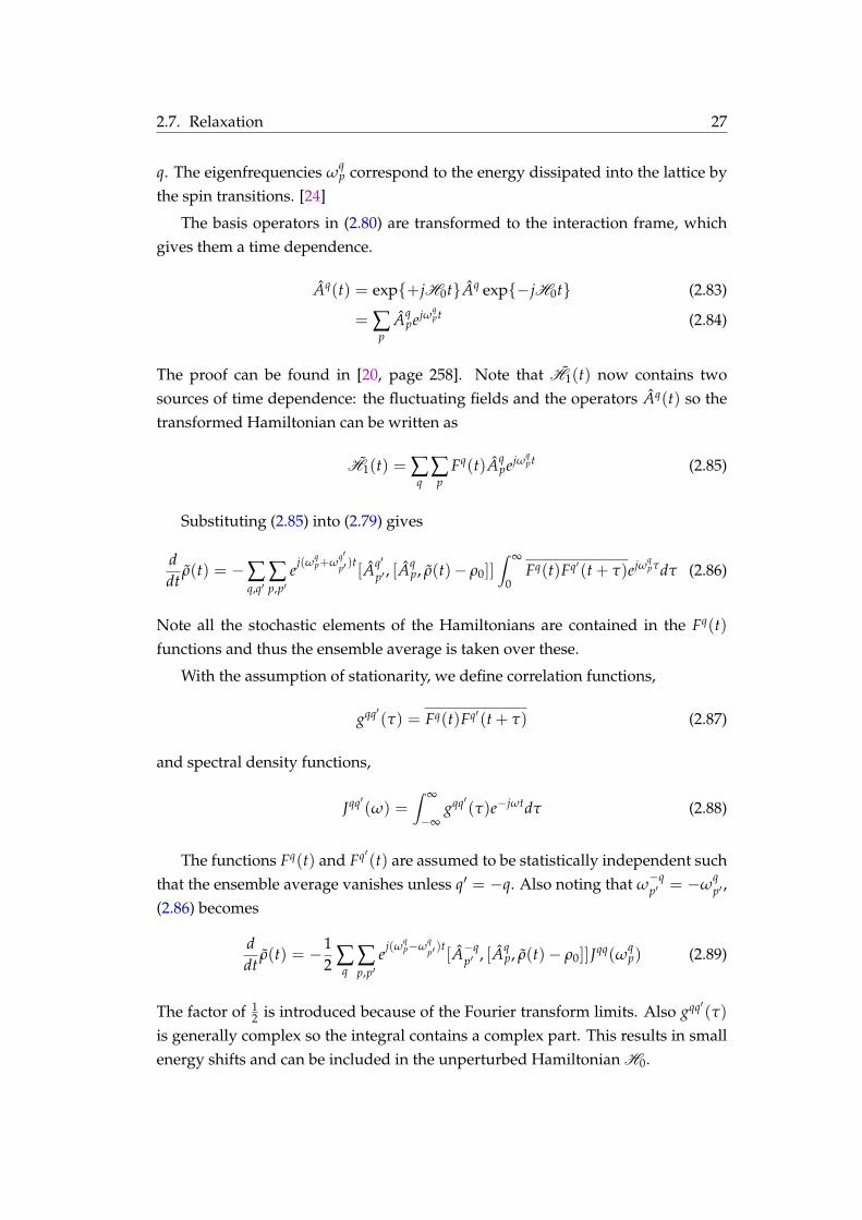
q. The eigenfrequencies ωqp correspond to the energy dissipated into the lattice by
the spin transitions. [2424]
The basis operators in (2.802.80) are transformed to the interaction frame, whichgives them a time dependence.
Aq(t) = exp+jH0tAq exp−jH0t (2.83)
= ∑p
Aqpejωq
pt (2.84)
The proof can be found in [2020, page 258]. Note that H1(t) now contains twosources of time dependence: the fluctuating fields and the operators Aq(t) so thetransformed Hamiltonian can be written as
H1(t) = ∑q
∑p
Fq(t)Aqpejωq
pt (2.85)
Substituting (2.852.85) into (2.792.79) gives
ddt
ρ(t) = −∑q,q′
∑p,p′
ej(ωqp+ω
q′p′ )t[Aq′
p′ , [Aqp, ρ(t)− ρ0]]
∫ ∞
0Fq(t)Fq′(t + τ)ejωq
pτdτ (2.86)
Note all the stochastic elements of the Hamiltonians are contained in the Fq(t)functions and thus the ensemble average is taken over these.
With the assumption of stationarity, we define correlation functions,
gqq′(τ) = Fq(t)Fq′(t + τ) (2.87)
and spectral density functions,
Jqq′(ω) =∫ ∞
−∞gqq′(τ)e−jωtdτ (2.88)
The functions Fq(t) and Fq′(t) are assumed to be statistically independent suchthat the ensemble average vanishes unless q′ = −q. Also noting that ω
−qp′ = −ω
qp′ ,
(2.862.86) becomes
ddt
ρ(t) = −12 ∑
q∑p,p′
ej(ωqp−ω
qp′ )t[A−q
p′ , [Aqp, ρ(t)− ρ0]]Jqq(ω
qp) (2.89)
The factor of 12 is introduced because of the Fourier transform limits. Also gqq′(τ)
is generally complex so the integral contains a complex part. This results in smallenergy shifts and can be included in the unperturbed Hamiltonian H0.

28 Chapter 2. Physics of magnetic resonance
Terms in which |ωqp − ω
qp′ | 0 are nonsecular, i.e., they do not affect the long-
time behaviour of the system because the rapidly oscillating factors ej(ωqp−ω
qp′ )t av-
erage to zero faster than relaxation occurs. If none of the eigenfrequencies are de-generate (more than one eigenoperator associated with a single eigenfrequency),only secular terms in which p = p′ are non-zero. This leads to
ddt
ρ(t) = −∑q
∑p
Jqq(ωqp)[A
−qp , [Aq
p, ρ(t)− ρ0]] (2.90)
Converting (2.902.90) back to the laboratory frame yields the modified Liouville-vonNeuman equation for relaxation,
ddt
ρ(t) = −j[H0, ρ(t)]− Γ (ρ(t)− ρ0) (2.91)
where the relaxation operator is
Γ(ρ) = ∑q
∑p
Jqq(ωqp)[A
−qp , [Aq
p, ρ]] (2.92)
2.7.2.4 Example
We now consider an example where the spins are coupled to a randomly fluctuat-ing lattice. Spin-spin coupling is not considered but a similar analysis could be per-formed for Hamiltonians that model the interactions discussed in the beginning ofthis section. This example serves to demonstrate how macroscopic relaxation rates(T1 and T2) can be derived from the equations of motion with appropriate Hamil-tonians. In our example a simple Hamiltonian is considered,
H1(t) = Fx(t) Ix + Fy(t) Iy + Fz(t) Iz (2.93)
which models random fluctuations of the angular moment operators. It is com-mon to examine the relaxation of the density matrix by explicitly calculating theelements as in [2525]; although, in this example, it is sufficient to following the pro-cedure outlined in Section 2.7.2.32.7.2.3. Noting that Fx, Fy and Fz are statistically inde-pendent we obtain the relaxation operator,
Γ(ρ) = Jxx(ω0)[ Ix, [ Ix, ρ]] + Jyy(ω0)[ Iy, [ Iy, ρ]] + Jzz(0)[ Iz, [ Iz, ρ]] (2.94)
We seek the evolution of the expected value of Ix and Iy representing the trans-verse magnetisation components and Iz representing the longitudinal magnetisa-

2.7. Relaxation 29
tion. The differential equation for the expectation of operator, Q, is
ddt〈Q〉 = d
dtTr(Qρ)= Tr
(ddt
ρ(t)Q)
(2.95)
Inserting the Liouville equation with relaxation derived in (2.912.91) gives,
ddt〈Q〉 = Tr
(−j[H0, ρ]− Γ(ρ)
)Q
(2.96)
We begin with the longitudinal magnetisation and compute 〈 Iz〉. In this casewe use the fact that Tr([H0, ρ]Iz) = 0 to simplify the general equation above to,
ddt〈 Iz〉 = −Tr
(Γ(ρ− ρ0) Iz
)(2.97)
= −Jxx(ω0)Tr([ Ix, [ Ix, ρ− ρ0]] Iz
)− Jyy(ω0)Tr
([ Iy, [ Iy, ρ− ρ0]] Iz
)− Jzz(0)Tr
([ Iz, [ Iz, ρ− ρ0]] Iz
) (2.98)
We let D = ρ− ρ0 and calculate the trace of each term above,
Tr([ Ix, [ Ix, D]] Iz
)= Tr
(( I2
x D + D I2x − 2 IxD Ix) Iz
)(2.99)
=12
Tr(
D Iz)− 2Tr
(D Ix Iz Ix
)(2.100)
=12
Tr(
D Iz)+
12
Tr(
D Iz)
(2.101)
= 〈 Iz〉 − 〈 Iz〉0 (2.102)
where 〈 Iz〉0 is the expected value of the Iz operator at thermal equilibrium. Thecomputations above have exploited the cyclic property of trace, the commutativityof I2
x and Iz and the relation Ix Iz Ix = − Iz/4. Similarly for the second term we have
Tr([ Iy, [ Iy, ρ− ρ0]] Iz
)= 〈 Iz〉 − 〈 Iz〉0 (2.103)
The third term is 0 which can be seen by expanding the commutator similarly tothe first term above. Combining these results gives
ddt〈 Iz〉 = − (Jxx(ω0) + Jyy(ω0))
(〈 Iz〉 − 〈 Iz〉0
)(2.104)
This is related to the classical Bloch time constant, T1, by
1T1
= Jxx(ω0) + Jyy(ω0) (2.105)

30 Chapter 2. Physics of magnetic resonance
Next we calculate the transverse magnetisation given by 〈 Ix〉 and 〈 Iy〉. Unlikethe longitudinal component Ix and Iy do not commute with H0 so the first term in(2.962.96) is not zero.
Tr−j[H0, ρ] Ix
= jω0Tr
([ Iz, ρ] Ix
)(2.106)
= jω0Tr([ Ix, Iz]ρ
)(2.107)
= ω0Tr(
Iyρ)
(2.108)
= ω0〈 Iy〉 (2.109)
The relaxation operator is composed of three terms which are evaluated below,
Tr([ Ix, [ Ix, ρ− ρ0]] Ix
)= 0 (2.110)
Tr([ Iy, [ Iy, ρ− ρ0]] Ix
)= 〈 Ix〉 (2.111)
Tr([ Iz, [ Iz, ρ− ρ0]] Ix
)= 〈 Ix〉 (2.112)
where we assume 〈 Ix〉0 = 0. Combining the results gives a differential equationfor 〈 Ix〉,
ddt〈 Ix〉 = ω0〈 Iy〉+ (Jyy(ω0) + Jzz(0)) 〈 Ix〉 (2.113)
Similar computations for 〈 Iy〉 can be performed.
ddt〈 Iy〉 = −ω0〈 Ix〉+ (Jxx(ω0) + Jzz(0)) 〈 Iy〉 (2.114)
These coupled equations clearly represent precession and relaxation of the trans-verse magnetisation. In this example we assume Jxx(ω0) = Jyy(ω0), which is rea-sonable for microscopic interactions. The relaxation is related to the classical Blochtime constant, T2, by
1T2
= Jyy(ω0) + Jzz(0) (2.115)
The transverse relaxation time is made up of two terms which have differentphysical meanings. The term Jyy(ω0) represents the non-secular contribution. Thisinvolves state transitions that are induced due to random fluctuations in the lat-tice. The frequency of this random fluctuation must match the energy differencebetween states, hence the J(ω0) term. The second term Jzz(0) represents the sec-ular contribution. This does not involve transitions with the lattice (also calledadiabatic relaxation). Instead, the random fluctuations in the z-direction, Fz(t),superimpose on the static B0 field to slightly alter the Larmor frequency of each

2.8. Summary 31
spin. This distribution of Larmor frequencies creates rapid dephasing. In MRI lit-erature, the classical model is often modified by introducing different isochromatsand integrating over a Lorentzian distribution to create the so-called T∗2 . In quan-tum mechanics, the spread is implicitly modelled by the stochastic nature of theinteraction Hamiltonian H1.
As mentioned at the start of this section, the previous analysis could be per-formed for more complicated Hamiltonians to model actual relaxation effects suchas dipole-dipole coupling and chemical shift anisotropy (CSA) relaxation. Onewould then expect physical parameters that define these Hamiltonians to appearin the various differential equations describing the behaviour of the ensemble.Such parameters may include the internuclear distance r, chemical shielding σ
or J-coupling J. We would also expect terms such as Jzz(2ω0) to appear, to modeldouble-quantum transitions. For example, [1515, page 537] states the transverse re-laxation time-constant for dipole-dipole relaxation as
1T2
=
(µ0γ2h4πr3
)2
3J(0) + 5J(ω0) + 2J(2ω0) (2.116)
We can interpret this to mean that T2 is parameterised by four parameters: r, J(0),J(ω0), and J(2ω0), which directly represent the physical parameters of the molec-ular environment.
This example demonstrates the underlying mechanisms of T1 and in particularT2 relaxation time, which is estimated in subsequent chapters of this thesis.
2.8 Summary
The physics behind spin systems and the generation of magnetisation is funda-mental to MRI. This chapter has presented a detailed description using both clas-sical and quantum mechanical theories. Phenomena such as thermal equilibrium,precession, control and relaxation have been described. In will be seen in the re-maining chapters, that accurate models of the spin dynamics is essential for imagereconstruction and advanced parameter estimation.


CHAPTER 3
Principles of magnetic resonanceimaging
Contents3.1 Introduction . . . . . . . . . . . . . . . . . . . . . . . . . . . . . . . . . 3434
3.1.1 Notation . . . . . . . . . . . . . . . . . . . . . . . . . . . . . . . 35353.2 Signal detection . . . . . . . . . . . . . . . . . . . . . . . . . . . . . . . 35353.3 Signal echoes . . . . . . . . . . . . . . . . . . . . . . . . . . . . . . . . 3838
3.3.1 Spin echoes and CPMG echoes . . . . . . . . . . . . . . . . . . 38383.3.2 Gradient echoes . . . . . . . . . . . . . . . . . . . . . . . . . . . 4040
3.4 Spatial encoding . . . . . . . . . . . . . . . . . . . . . . . . . . . . . . 41413.4.1 Slice selection . . . . . . . . . . . . . . . . . . . . . . . . . . . . 42423.4.2 Frequency encoding . . . . . . . . . . . . . . . . . . . . . . . . 43433.4.3 Phase encoding . . . . . . . . . . . . . . . . . . . . . . . . . . . 44443.4.4 k-space . . . . . . . . . . . . . . . . . . . . . . . . . . . . . . . . 4444
3.5 Basic sequences . . . . . . . . . . . . . . . . . . . . . . . . . . . . . . . 45453.5.1 Cartesian . . . . . . . . . . . . . . . . . . . . . . . . . . . . . . . 45453.5.2 Radial . . . . . . . . . . . . . . . . . . . . . . . . . . . . . . . . 47473.5.3 EPI . . . . . . . . . . . . . . . . . . . . . . . . . . . . . . . . . . 4949
3.6 Image reconstruction . . . . . . . . . . . . . . . . . . . . . . . . . . . . 50503.6.1 Direct Fourier . . . . . . . . . . . . . . . . . . . . . . . . . . . . 50503.6.2 Gridding . . . . . . . . . . . . . . . . . . . . . . . . . . . . . . . 51513.6.3 Iterative . . . . . . . . . . . . . . . . . . . . . . . . . . . . . . . 5252
3.7 Properties of MRI signals . . . . . . . . . . . . . . . . . . . . . . . . . 53533.7.1 Signal-to-noise ratio . . . . . . . . . . . . . . . . . . . . . . . . 53533.7.2 Signal processing challenges . . . . . . . . . . . . . . . . . . . 5555
33

34 Chapter 3. Principles of magnetic resonance imaging
3.1 Introduction
A magnetic resonance scanner is composed of many components that worktogether to produce the final image. Figure 3.13.1 illustrates the main compo-
nents of an MRI system. The scanner consists of a main magnet, spatial encodinggradients, an RF pulse generator to control the transmit coils and signal detectionhardware including RF receive coils and analog-to-digital converters.
The main magnet is used to generate a large, static and homogeneous magneticfield. In the presence of this magnetic field, the signal behaves according the phys-ical principles discussed in Chapter 22. The physics of spin systems is fundamentalto the operation of the scanner.
All hardware components are controlled with an acquisition protocol known asa ‘sequence’. The sequence contains a list of instructions and their precise timing;it can be considered the main input into the system.
In general only the transverse magnetisation is detectable so the first step inmost MRI protocols is to excite the spin system to tip the magnetisation into thetransverse plane. As described in the previous chapter, this can be achieved usingan RF pulse tuned to the resonant frequency of the spin system. These pulsesare controlled with RF hardware consisting of a pulse generator, amplifier andtransmit coils.
Spatial information is encoded into the underlying signal using a set of mag-netic fields known as gradients. These encoding gradients modulate the signal ina spatially dependent manner, which is later used to resolve the observed signal toform an image.
Acquisi'on Sequence
MRI System
Spa'al Encoding Gradients
RF Pulse Generator
Signal Detec'on Image Reconstruc'on Spin Physics
Main Magnet
Figure 3.1: Overview of the main components in an MRI machine. The machinecan be viewed as a system that inputs a list of precisely timed instructions (knownas a ‘sequence’) and outputs raw data, which is used to produce the final image.

3.2. Signal detection 35
Table 3.1: Common notation used in Chapter 33
Symbol Quantity Units
Φ Magnetic flux Wbc Coil sensitivitym Magnetisation vectorV Induced voltage Vb z-Component of the magnetic field Tg Gradient vector T/mTp Duration of pulse sτE Echo time sTacq Acquisition time (one readout) sT Sampling period sSNR Signal-to-noise ratioBW Acquisition bandwidth Hz
Signal detection involves analog-to-digital conversion of the voltage receivedon the RF coils. Receive RF coils are either volume coils or surface coils, dependingon the application. Transmit and receive coils can be separate coils or combinedinto a single coil although there are two distinct roles: transmit coils excite thespins and rotate the magnetisation vector and receive coils detect the transversemagnetisation. Finally, the acquired signal is converted to an image, a processknown as image reconstruction.
This chapter introduces the main components and basic principles of MRI. Ad-ditionally, the generation of echoes and the notion of k-space is introduced andused to describe common sequences. Finally, image reconstruction is consideredfrom a general inverse problem perspective. The concepts outlined in this chapterare the foundation of the novel contributions in subsequent chapters of this thesis.
3.1.1 Notation
Table 3.13.1 lists the important symbols used in this chapter. Although the list is notexhaustive, it includes most quantities of interest.
3.2 Signal detection
Signal detection is the process of converting nuclear magnetisation into an electri-cal signal. The voltage induced on an RF receive coil, V(t), is governed by Fara-

36 Chapter 3. Principles of magnetic resonance imaging
day’s law of induction:
V(t) = −dΦB(t)dt
(3.1)
The magnetic flux through a coil is defined as
ΦB(t) =∫
objm(x, t) · c(x)dx (3.2)
where m is the magnetisation and c is the coil sensitivity. Combining (3.13.1) and (3.23.2)gives a received voltage of
V(t) = − ∂
∂t
∫obj
m(x, t) · c(x)dx (3.3)
We adopt the common notation defined in (2.432.43) and let mxy(x, t) = mx(x, t) +jmy(x, t). Since quadrature detection is used we can represent the coil sensitivityvector as
c(x) = c(x)
1j0
(3.4)
The received voltage is demodulated to baseband to extract the underlyingsignal of interest, s(t),
s(t) = V(t)ejω0t (3.5)
= −(
∂
∂t
∫obj
c(x)mxy(x, t)dx)
ejω0t (3.6)
During detection, the transverse magnetisation, mxy, is undergoing precessionand relaxation as described in Chapter 22. The general form is
mxy(x, t) = M0(x)e−j(ω0t+φ0)ejφ(x,t)e−t/T∗2 (x). (3.7)
where M0 is the initial magnetisation strength, φ0 is the initial signal phase, φ(x, t)is the spatial encoding phase and T∗2 is the free induction decay (FID) time. Thisleads to the detected signal,
s(t) = −(
∂
∂t
∫obj
c(x)M0(x)e−j(ω0t+φ0)ejφ(x,t)e−t/T∗2 (x)dx)
ejω0t (3.8)
Simplifications of this general form are possible by making a series of assump-

3.2. Signal detection 37
tions. It is useful to invoke a different set of assumptions for different problemsaddressed in this thesis.
A3.1 The magnetisation precession is much faster than any time-dependent spa-tial encoding, inhomogeneity or relaxation processes. That is, we assume
ω0 ∂φ(x, t)
∂t, ω0
1T∗2 (x)
. (3.9)
In this case,
s(t) ≈ jω0
∫obj
c(x)M0(x)ejφ0 ejφ(x,t)e−t/T∗2 (x)dx (3.10)
Notice the rotating ω0 component is removed by the demodulation.
A3.2 The transverse magnetisation has zero phase initially. This corresponds toan initial bulk magnetisation on the x-axis.
A3.3 The ω0 scaling factor can be considered constant across different experimentsand hence we can arbitrarily set it to unity. Additionally the multiplicationby j creates a global phase shift of π, which we ignore without loss of gener-ality.
A3.4 Signal amplitude is constant during acquisition. In other words, the relax-ation process occurs on a timescale much longer than the time of interest.During acquisition we have
e−t/T∗2 (x) ≈ e−τE/T∗2 (x) (3.11)
Combining assumptions A3.1A3.1 to A3.4A3.4 the received signal can be written as
s(t) ≈∫
objc(x)M0(x)e−τE/T∗2 (x)ejφ(x,t)dx (3.12)
A3.5 The coil sensitivity is uniform and hence set to unity, i.e., c(x) = 1. Neglect-ing receiver phase, this is a reasonable assumption for a birdcage coil [2626].Combining all previous assumptions, A3.1A3.1 to A3.5A3.5, yields,
s(t) ≈∫
objm(x)ejφ(x,t)dx (3.13)
where
m(x) = M0(x)e−τE/T∗2 (x) (3.14)

38 Chapter 3. Principles of magnetic resonance imaging
3.3 Signal echoes
Signal echoes are fundamental to some contrast mechanisms and form the basisof many MR imaging techniques. Due to the local field inhomogeneities or an ap-plied gradient field the imaged object consists of a broad range of isochromats. Thatis, the spins are precessing at different frequencies centred about the resonancefrequency. The distribution of frequencies mean that spins dephase very quicklyrelative to the intrinsic relaxation processes, resulting in rapid signal decay. It ispossible to reverse the dephasing due to inhomogeneity to partially recover thesignal, which is known as an ‘echo’. An echo can be generated in two ways:
Gradient echo The distribution of frequencies is flipped by reversing the appliedgradient field.
Spin echo The spins are rotated 180 using an RF pulse.
These echo generation mechanisms will be described in detail in the followingsections.
3.3.1 Spin echoes and CPMG echoes
The generation of a spin echo was first demonstrated in [2727] and since then, mostMR imaging was performed by generating an echo some time after the initial ex-citation.
Figure 3.23.2 illustrates the generation of a spin echo. Figure 3.2a3.2a shows the bulkmagnetisation at time t = 0, just after a 90 RF pulse. The spins begin to precessat slightly different speeds until τ seconds later when “faster” isochromats have alarger phase as shown in Figure 3.2b3.2b. At time τ a 180 pulse is applied to flip thevectors about the y-axis (Fig. 3.2c3.2c), causing the faster isochromats to lag the slowerones. After another τ seconds, the faster spins will have caught the slower onesand an echo is formed. The signal over the duration τE− Tacq/2 ≤ t ≤ τE + Tacq/2is
s(t) =∫
objM0(x)e−t/T2(x)e−|t−τE|/T′2(x)e−jk(t)·xdx (3.15)
where T′2 captures the width of the off-resonance distribution as described in Chap-ter 22.
The process described by Figures 3.23.2 and 3.33.3 can be repeated by applying atrain of 180 RF pulses spaced 2τ apart. In this case successive echoes will begenerated at times, t = 2τ, 4τ, . . . , 2Neτ. This sequence was first introduced byCarr and Purcell in [2828] and modified by Meiboom and Gill in [2929] and as such

3.3. Signal echoes 39
y
z
x
(a) t = 0
y
z
x
(b) t = τ−
y
z
x
(c) t = τ+
y
z
x
(d) t = 2τ
Figure 3.2: Formation of a spin echo illustrated by two vectors representing dif-ferent isochromats. The ‘fast’ isochromat is indicated in blue and gains a positivephase at time t = τ− relative to the ‘slow’ isochromat in red. After a 180 pulse attime t = τ+ the fast isochromat lags the slow isochromat. An echo is formed whenthe spins have the same phase again at t = 2τ.
90
Signal
RF
e−t/T2
FID
180
τ τ
Figure 3.3: Timing diagram depicting the generation of a spin echo.

40 Chapter 3. Principles of magnetic resonance imaging
90
Signal
RF
e−t/T2FID
180
τ τ
180
τ τ
180
τ τ
180
τ τ
Figure 3.4: Timing diagram illustrating a CPMG sequence.
it is known as the CPMG sequence. Figure 3.43.4 demonstrates the timing of the RFpulses and subsequent echoes. The spin system undergoes spin-spin relaxationwhich represents a loss of coherence that cannot be recovered. As such the echoamplitudes are weighted by e−2τn/T2 . This weighting makes the CPMG sequencevery efficient for estimating the T2 relaxation time from a set of echo amplitudes.The problem of T2 estimation is explored in detail in Chapters 44 and 55.
3.3.2 Gradient echoes
Gradient fields are crucial for spatial encoding and they typically generate signalechoes as a consequence. During free induction decay (FID) the application of agradient field over the sample creates a distribution of isochromats precessing atdifferent frequencies. Analogous to the spin echo case, this distribution causes thespins to dephase and the overall signal decays much faster than the FID relaxation.This dephasing can be recovered by reversing the sign of the applied gradient field.The spins will be rephased after the reversed gradient has been applied for thesame duration as the initial gradient, resulting in an echo. Figure 3.53.5 illustrates thegeneration of a gradient echo.
It is important to note that a gradient echo cannot reverse any dephasing dueto underlying field inhomogeneity. As such, the echo amplitude will be weightedby the signal strength of the FID without gradients. The gradient echo occurs attime τE when the encoding phase φ = 0. Under assumptions A3.1A3.1 to A3.5A3.5, thesignal intensity during the echo is easily derived from (3.133.13) as
s(t) =∫
objM0(x)e−τE/T∗2 (x)ejφ(x,t)dx, (3.16)
which highlights the dependance on T∗2 .

3.4. Spatial encoding 41
α
Signal
RF
g
FIDEffective decay
Figure 3.5: Timing diagram depicting the generation of a gradient echo.
3.4 Spatial encoding
Spatial encoding is the process of encoding the positions of different magnetisa-tion vectors in an object. This encoding enables image reconstruction and is fun-damental to all MRI techniques. The received signal was derived in Section 3.23.2under assumptions A3.1A3.1 to A3.5A3.5. In the general case, spatial encoding is achievedby creating a phase distribution, φ, that is dependent on both time and space.
s(t) =∫
objm(x)ejφ(x,t)dx (3.17)
The phase is related to the encoding magnetic field by
φ(x, t) = −γ∫ t
0b(x, τ)dτ. (3.18)
The encoding field is the superposition of the field generated by each gradient coil.For three linear gradients shown in Figure 3.63.6 the total encoding field is
b(x, t) = gx(t)x + gy(t)y + gz(t)z (3.19)
For simplicity we let g(t) =[gx(t), gy(t), gz(t)
]T, thus the total field can bewritten as
b(x, t) = g(t) · x, (3.20)
where a · b denotes the inner product. Substituting into (3.183.18) the encoding phase

42 Chapter 3. Principles of magnetic resonance imaging
(a) (b) (c)
Figure 3.6: Linear encoding gradients for the three imaging dimensions illustratingthe spatially-varying field offset imposed by each gradient. The maximum field ofeach gradient is given by B = GL/2 where G is the gradient strength (T/m) and Lis the field of view (m).
is related to the gradient waveforms by
φ(x, t) = −γ∫ t
0g(τ)dτ · x. (3.21)
3.4.1 Slice selection
The first step in common two dimensional imaging sequences is to excite a thinslice of the object. This can be achieved by applying a gradient field and frequencyselective RF pulse simultaneously. To select a slice in the x-y plane, the gradientfield b(z) = zGz is first applied. The precession frequency, ω, of spins within theobject becomes dependent on the z-coordinate,
ω(z) = ω0 + γGzz (3.22)
where ω0 is the Larmor frequency due to the main magnetic field, Gz is the mag-nitude of the gradient change and z is the position along the z-axis.
After applying the gradient field the desired spins are excited using a bandlim-ited RF pulse oscillating at the required Larmor frequency. For example, an RFpulse resonating at ω(z1), with a bandwidth of ∆ω will excite a slice of the ob-ject between z = z1 − ∆z/2 and z = z1 + ∆z/2 where ∆z is the slice thickness.Ideally, only spins in this slice will be rotated into the transverse plane and con-tribute to the received signal. In practice, however, the transverse magnetisation

3.4. Spatial encoding 43
z
ω
∆ω
∆z
ω = γzGz
Figure 3.7: Slice selection diagram representing the spatially dependence fre-quency and an example slice.
follows a smooth slice profile and some “leakage” will occur, dependent on theRF pulse shape. Figure 3.73.7 illustrates the position dependent precession frequencyand an example slice excited from a frequency selective RF pulse. Notice that theslice thickness is linearly related to the gradient strength (Gz) and bandwidth (∆w).This procedure can be repeated for different slices to encode the slice dimension.The remaining two dimensions can be encoded using a combination of frequencyand phase encoding discussed below.
3.4.2 Frequency encoding
Frequency encoding is achieved by applying constant gradient over the entire timeinterval,
g(t) = gf, t > 0 (3.23)
The encoding phase in this case is
φ(x, t) = −γ∫ t
0g(τ)dτ · x (3.24)
= −γtgf · x (3.25)
The received signal becomes
s(t) =∫
objm(x)e−jγtgf·xdx (3.26)
The signal can be interpreted as a 1D projection of the object, characterised by thegradient gf. Intuitively, we can obtain different projections by altering the gradientand acquiring the signal again.

44 Chapter 3. Principles of magnetic resonance imaging
3.4.3 Phase encoding
Suppose a gradient field gp is briefly applied to the sample just after the RF pulse.
g(t) =
gp, 0 ≤ t ≤ Tp;
0, otherwise.(3.27)
During the gradient duration (0 ≤ t ≤ Tp) the received signal is frequencyencoded as discussed above. For t > Tp the signal at every point returns to preces-sion at ω0 but has acquired a spatially dependent phase offset of
φ(x) = −γTpgp · x. (3.28)
The acquired signal with phase encoding is
s(t) =∫
objm(x)e−jγTpgp·xdx, t > Tp. (3.29)
Notice the right hand side of (3.293.29) is independent of time but the magnetisationhas been modulated with a phase characterised by the gradient, gp, and the dura-tion, Tp.
3.4.4 k-space
Frequency and phase encoding discussed above can be described in a commonframework using the notion of k-space [3030, 3131]. The key point is to make the fol-lowing substitution,
k(t) = γ∫ t
0g(τ)dτ (3.30)
where γ = γ/2π. The encoding phase in (3.213.21) becomes linear in both k and xwith φ = −2πk · x and the signal is written as
s(k) =∫
objm(x)e−j2πk·xdx (3.31)
This can be recognised as a multi-dimensional Fourier transform, where the spatialfrequency domain is referred to as k-space. The definition in (3.303.30) highlights theimportant relationship between the applied gradient fields and the position in k-space. We can interpret frequency encoding discussed above as moving throughk-space with a constant velocity whereas phase encoding can quickly move the k-space position a short distance. Importantly, different gradient waveforms lead to

3.5. Basic sequences 45
different trajectories through k-space.
3.5 Basic sequences
In this section we examine some common sequences for two dimensional imag-ing. Prior to encoding, a gradient is applied in the z direction in combinationwith a frequency selective RF pulse to excite a slice of spins as described in Sec-tion 3.4.13.4.1. Thus spatial encoding is performed over the remaining two dimensionsand k-space vectors are defined in R2. Sequences are defined by the timing of thegradient systems, RF pulses and the analog-to-digital converter (ADC).
3.5.1 Cartesian
The most common sampling strategies are based on a Cartesian trajectory. Thistype of trajectory starts with phase encoding using constant gradients for an initialperiod, Tp,
g(t) =
[Gx
Gy
], t < Tp (3.32)
Using (3.303.30) the k-space position after time Tp will be kA = γTp [Gx, Gx]T. To
generate an echo a 180 pulse is applied, which inverts the phase of the signal.In terms of k-space, this is equivalent to the position being reflected about theorigin so immediately after the pulse, kB = γTp [−Gx,−Gx]
T. Frequency encodingis achieved by applying a constant gx gradient during readout. This moves thetrajectory along the kx dimension of k-space as displayed in Figure 3.8a3.8a. Duringthe readout period we have,
k(t) = γ
[(t− τE)Gx
GyTp
], |t− τE| < Tacq/2 (3.33)
The ky gradient moment is set up during the initial phase encode and is constantduring readout. The readout gradient, Gx, is constant for all excitations causingrepetitive evolution of the kx coordinate. The process is repeated for different val-ues of Gy to define different horizontal lines across the kx-ky plane as shown inFigure 3.8b3.8b. Figure 3.93.9 displays a sequence diagram for the Cartesian trajectory,which illustrates the timing and function of the different subsystems.
Cartesian trajectories are popular since they are relatively insensitivity to fieldinhomogeneities and gradient nonlinearities [3232]. Further, images are easy to re-

46 Chapter 3. Principles of magnetic resonance imaging
kx
ky
(a)
kx
ky
(b)
Figure 3.8: The k-space sampling pattern for a Cartesian spin echo trajectory illus-trating (a)(a) a single line consisting of a phase encode, refocusing pulse and readout;and (b)(b) the complete sampling pattern from multiple excitations.
90
gz
gx
gy
180
τE
ADC
RF
Figure 3.9: Sequence diagram for a Cartesian spin echo trajectory illustrating asingle excitation, phase encode, refocusing pulse and readout.

3.5. Basic sequences 47
construct using the discrete Fourier transform (DFT) as discussed in Section 3.63.6.
3.5.2 Radial
A simple radial trajectory begins much like the Cartesian trajectory described above.Specifically, a phase encoding gradient is applied such that the k-space position af-ter time Tp will be kA = γTp
[Gx, Gy
]T as described above. A refocusing pulseis applied to move k-space position to kB = −kA. Samples are collected whenthe constant gradients are switched on again in the period τE − Tacq/2 ≤ t ≤τE + Tacq/2. The main difference from a Cartesian trajectory is that both gradi-ents (gx and gy) are applied during the readout. The k-space trajectory during thisperiod is
k(t) = kB + γ(t− (τE − Tacq/2))
[Gx
Gy
], |t− τE| < Tacq/2 (3.34)
The phase encoding defining point kB is only dependent on Gx, Gy and Tp, nottime during the readout. This reveals the important property that phase encodingonly affects the starting point of the k-space trajectory.
With careful selection of the phase encoding duration such that Tp = Tacq/2,we can reparameterise (3.343.34) as
k(t) = C(t− τE)
[cos θ
sin θ
], |t− τE| < Tacq/2 (3.35)
where θ = arctan(Gy/Gx) is the angle of the trajectory and C = γ√
G2x + G2
y de-fines the trajectory speed. This process is illustrated in Figure 3.10a3.10a. Sufficient sam-pling of k-space is achieved by repeating the above process for different angles, θ,by defining appropriate values of Gx and Gy. The complete sampling pattern inshown in Figure 3.10b3.10b. Figure 3.113.11 displays a sequence diagram for the radialtrajectory, which illustrates the timing of the gradient, RF and ADC systems.
Radial sampling in MRI is a direct analog to standard x-ray imaging and conse-quently it inherited a broad range of the prior knowledge concerning image recon-struction. Indeed the first MR images were produced using radial projections [3333].In general, however, the reconstruction algorithm is more complex than Fourier re-construction of Cartesian samples. Another difficulty is that off-resonance effectsdue to field inhomogeneities create blurring along the radial direction whereasFourier imaging is affected by shifts in the readout direction resulting in geomet-ric distortion [3232, 3434, 3535]. Despite these shortcomings, radial imaging remains use-

48 Chapter 3. Principles of magnetic resonance imaging
kx
ky
(a)
kx
ky
(b)
Figure 3.10: The k-space sampling pattern for a radial trajectory illustrating (a)(a) asingle spoke consisting of a phase encode, refocusing pulse and readout; and (b)(b)the complete sampling pattern from multiple excitations.
90
gz
gx
gy
180
τE
ADC
RF
Figure 3.11: Sequence diagram for a radial trajectory illustrating a single excitation,phase encode, refocusing pulse and readout.

3.5. Basic sequences 49
kx
ky
Figure 3.12: The k-space sampling pattern for a Cartesian EPI trajectory illustrat-ing the initial phase encode and rapid trajectory through k-space from a singleexcitation.
ful for specialised applications. Since the readout can start immediately after theslice select gradient, this technique is useful to image tissue with short T2 or T∗2 .Another advantage of radial imaging is the relative insensitivity to subject motionmaking it useful for dynamic imaging applications [3636].
3.5.3 EPI
Echo planar imaging (EPI) was first introduced in [3737] and later modified to pro-duce Cartesian trajectories [3838, 3939]. Although the final sampling trajectory is sim-ilar to the Cartesian spin echo in Figure 3.8b3.8b, the underlying mechanism is dif-ferent. Firstly, the trajectory is acquired with a single excitation and belongs toclass of imaging techniques referred to as “single-shot”. Secondly, the echoes aregenerated by switching the gradient polarity rather than a 180 refocusing pulse.
A simple EPI trajectory is shown in Figure 3.123.12, generated from the sequencediagram in Figure 3.133.13. The trajectory begins by exciting a slice of the object torotate the magnetisation through a flip angle, α. As described above, prephasinggradients are applied to move the trajectory from the centre to the edge of the sam-pled k-space. Next, a series of echoes is generated by rapidly switching the polarityof the readout gradient. This moves the k-space trajectory back and forth along thehorizontal direction. At the end of each line a brief phase encode gradient is ap-plied to move the trajectory a small amount in the vertical direction in preparationfor the next readout line. The final result is a Cartesian k-space sampling patternacquired in under 50 ms, orders of magnitude faster than traditional spin echotechniques [3939]. EPI imaging is insensitive to subject motion since the acquisitionoccurs on a shorter time scale than typical motion [4040]. Disadvantages include anincreased risk of peripheral nerve stimulation due to the rapidly switching gra-

50 Chapter 3. Principles of magnetic resonance imaging
α
gz
gx
gy
ADC
RF
Figure 3.13: Sequence diagram for a Cartesian EPI trajectory illustrating the timingof the single excitation pulse followed by phase encoding and readout gradients.
dients [4141, 4242] and sensitivity to magnetic field inhomogeneity and the associateddephasing [4343].
The EPI trajectory will be important in Chapter 66 and is the basis of our trajec-tory design for higher dimensional encoding schemes.
3.6 Image reconstruction
Image reconstruction is the process of generating an image from the measured MRsignal. In the simplest case, the image reconstruction problem can be described asfollows,
Find m(x)
Given s(ki) =∫
objm(x)e−j2πki ·xdx, ki ∈ K
(3.36)
The difficulty of this problem is revealed when we consider the preceding discus-sion regarding the inherent tradeoffs in MRI data.
The remainder of this section describes some commonly used reconstructionalgorithms.
3.6.1 Direct Fourier
We consider the reconstruction of a 1D function to illustrate the method, althoughthe theory is easily extended to 2D or 3D functions. Fourier reconstruction using

3.6. Image reconstruction 51
the DFT is suitable when samples are collected at a finite number of regularlyspaced k-space locations [4444]. That is,
K = i∆k, −N/2 ≤ i ≤ N/2− 1 (3.37)
Let s[i] = s(i∆k) denote the measurements. A common reconstruction is onethat satisfies the minimum-norm constraint. In this case the image is reconstructedusing a truncated Fourier series,
m(x) = ∆kN/2−1
∑i=−N/2
s[i]ej2πi∆kx, |x| < 1∆k
(3.38)
The reconstructed image function, m(·), is inherently bandlimited due to the trun-cation of its Fourier series. That is, (F m)(k) = 0 for |k| > (N/2)∆k. Nyquistsampling criterion states that this image function can be uniquely recovered fromsamples, m[n] = m(n∆x), provided the pixel size, ∆x, satisfies
∆x ≤ 1N∆k
(3.39)
Sampling (3.383.38) at the Nyquist limit gives,
m[n] = ∆kN/2−1
∑i=−N/2
s[i]ej2πin/N (3.40)
This can be recognised as the DFT of the measurements and as such this techniqueis called the direct DFT reconstruction.
3.6.2 Gridding
Gridding is used when the set K of k-space points are not regularly spaced inCartesian coordinates. A simple approach in this case is to interpolate the mea-sured points into a regular grid and then perform the direct DFT reconstructiondescribed above. Let s(k) be a sum of delta functions weighted by the measure-ments,
s(k) = ∑ki∈K
s(ki)δ(k− ki) (3.41)

52 Chapter 3. Principles of magnetic resonance imaging
These samples are convolved with an interpolation function, C, and sampled atregularly spaced points defined in the set L,
s[i] = (s ∗ C)(ki), ki ∈ L (3.42)
This sequence can now be reconstructed using a DFT.
3.6.3 Iterative
An alternative approach to image reconstruction is to formulate the problem as amatrix inversion. The signal equation is written as
s = Em (3.43)
where s is a vector of measurements, E is the encoding matrix and m is a vector ofunknown magnetisations. This formulation allows us to specify an arbitrary en-coding scheme, which may incorporate multiple receive coils, non-Cartesian tra-jectories or field inhomogeneity correction. Including these features into a Fourierreconstruction is not straightforward.
Reconstruction of a 256× 256 image using fully sampled data from a 32 channelreceive coil array has an encoding matrix with ∼1011 complex-valued elements.For double precision this would require approximately 2200 GB of memory. Inaddition to practical issues concerning memory, a direct inverse requires O(N3)
computations where N = 256× 256. Even with the dramatic increase in comput-ing power of modern computers, a direct matrix inversion of (3.433.43) is infeasiblefor clinical applications. For these reasons we consider two iterative algorithms tosolve (3.433.43). Both methods only require a single row of the encoding matrix at anygiven time and therefore avoid storing entire matrix in memory.
The first algorithm examined is the Kaczmarz iterative projection algorithm[4545] otherwise known as the Algebraic Reconstruction Technique (ART) [4646]. Thealgorithm is described in Algorithm 3.13.1. This method has been proven to convergeto the minimum norm least squares solution for sufficiently small step sizes [4747].Further, it is relatively simple to include prior information into the reconstructionalgorithm. In the case of Gaussian prior and noise distributions, the Kaczmarz al-gorithm converges to a regularised solution equivalent to the Bayesian maximuma posteriori (MAP) estimate [4747].
Another iterative method is the conjugate gradient (CG) algorithm [4848]. This al-gorithm was used in [4949] for reconstruction of parallel imaging data with arbitrarytrajectories. Instead of solving (3.433.43) directly the CG algorithm solves E′s = E′Em.

3.7. Properties of MRI signals 53
Algorithm 3.1: Algebraic Reconstruction TechniqueInput: s – signal, E – encoding matrix, N – number
of measurements, P – number of iterationsParams: λ – step sizeOutput: m – estimate
1 for n← 0, . . . , P do2 for i← 1, . . . , N do3 Assign the ith row of E to ai4
mn+1 ← mn + λsi − 〈ai, mn〉‖ai‖2 a∗i
5 Return estimate: m← mP
The algorithm is described in Algorithm 3.23.2. The algorithm only requires a sin-gle row of the encoding matrix at a time and has been proven to converge to thepseudo-inverse solution in a finite number of iterations [5050].
Both the conjugate gradient algorithm and algebraic reconstruction techniqueare used extensively to reconstruct data resulting from the nonlinear encodingschemes examined in Chapters 77 and 66.
3.7 Properties of MRI signals
The reconstruction algorithms in Section 3.63.6 were developed without consideringmeasurement noise. In reality, measurements are corrupted with thermal noise,which ultimately limits the imaging performance. Indeed the term ‘reconstruction’should perhaps be replaced with ‘estimation’, since we can only extract informa-tion from the measurements up to the level of noise. This section explores some ofthe ramifications of the stochastic nature of the measurements.
3.7.1 Signal-to-noise ratio
The thermal noise variance, σ2thermal, in an imaging experiment is given by the fol-
lowing relationship, first observed by Johnson [5151] and explained by Nyquist [5252],
σ2thermal = 4KB Ts RBW (3.44)
where KB is Boltzmann’s constant, Ts is the system temperature, R is the resistanceand BW is the acquisition bandwidth.

54 Chapter 3. Principles of magnetic resonance imaging
Algorithm 3.2: Conjugate Gradient ReconstructionInput: s – signal, E – encoding matrix, P – number
of iterationsOutput: m – estimate
1 m0 ← 02 p← Es3 r0 ← Es4 for n← 0, . . . , P do5
q← E′Ep
mn+1 ← mn +r∗nrn
p∗qp
rn+1 ← rn −r∗nrn
p∗qq
p← rn+1 +r∗n+1rn+1
r∗nrnp
6 Return estimate: m← mP
The signal strength, s, is proportional to the square of the main magnetic fieldstrength, i.e., s ∝ B2
0. However, it has been found that the resistance in (3.443.44) isfrequency dependent, which results in the relation, R ∝ B0 [5353]. Thus the signal-to-noise ratio (SNR), defined as SNR = s/σthermal, has the following relationship tofield strength [5454],
SNR ∝ B0 (3.45)
The relationships in (3.443.44) and (3.453.45) mean the SNR for Fourier imaging is in-trinsically linked to the acquisition parameters [5353]. In particular,
SNR/voxel ∝B0 ∆x∆y∆z
√Navg√
BWNx Ny Nz
(3.46)
where ∆x, ∆y and ∆z define the voxel dimensions, Nx, Ny and Nz are the numberof voxels in each dimension and Navg is the number of signal averages. SinceBW = 1/Tacq the SNR has the following relationship to the readout parameters,
SNR/voxel ∝ B0 ∆x
√Tacq. (3.47)
The final SNR of an image is further influenced by physiological noise, systematicerrors and reconstruction algorithm.

3.7. Properties of MRI signals 55
3.7.2 Signal processing challenges
The difficulty of many MRI problems is revealed when we consider the ideal so-lution from a users perspective. For both image reconstruction and parameterestimation problems, the user wants:
• fast acquisition times
• high resolution
• high SNR
• no image artifacts or bias
These are conflicting requirements for MRI data. For example, a fast acquisitiontime is often achieved by obtaining fewer measurements. On one hand, acquisitionis limited by the signal relaxation, on other, gradient switching constraints are im-posed due to hardware limitations and safety concerns regarding peripheral nervestimulation. These constraints limit the amount of k-space that can be covered ina fixed time; conversely, reducing the imaging time is achieved with fewer k-spacemeasurements.
Increasing the resolution of the reconstruction is equivalent to seeking a higherdimensional approximation of the underlying function. Processing a very highdimensional signal is difficult, even with the increase in modern computing power.When the number of measurements is limited, this reconstruction requires someform of prior knowledge for stable signal recovery in the presence of noise.
Prior knowledge is used to constrain the reconstruction, which is the basis ofmany state-of-the-art techniques, such as high resolution MR angiography [5555]and dynamic cardiac imaging [5656]. Although helpful, too much emphasis on priorknowledge leads to reconstruction artifacts or bias.
Tradeoffs are pervasive and cannot be avoided. Some typical tradeoffs and aresummarised below:
↑ resolution ⇔ ↑ signal dimension↓ acquisition time ⇔ ↓ number of measurements
↑ SNR ⇔ ↓ resolution↓ bias ⇔ ↓ reconstruction constraints
With this in mind, the ideal requirements above translate to the following sig-nal processing problem: Reconstruct a very large dimensional function from a smallnumber of noisy measurements without any prior knowledge about the function. Clearly,no solution will be adequate for a realistic class of functions. We are forced find acompromise between requirements that is suitable for a particular application.

56 Chapter 3. Principles of magnetic resonance imaging
The difficulty of the problem necessitates the need for accurate signal mod-els that capture the deterministic effects on the measurements. Only with pre-cise models can the desired quantities be distinguished from random noise. Thisestimation-theoretic perspective is adopted for the remainder of this thesis and wewill see that it leads to new techniques that push the boundaries of current MRItechnology.

Part II
Quantitative MRI
57

CHAPTER 4
Estimation of relaxation rates inthe presence of image distortion
Contents4.1 Introduction . . . . . . . . . . . . . . . . . . . . . . . . . . . . . . . . . 5959
4.1.1 Notation . . . . . . . . . . . . . . . . . . . . . . . . . . . . . . . 6060
4.2 Image distortion due to relaxation . . . . . . . . . . . . . . . . . . . . 6161
4.2.1 Spatial filter interpretation . . . . . . . . . . . . . . . . . . . . . 6262
4.2.2 Filter kernel approximation . . . . . . . . . . . . . . . . . . . . 6666
4.3 Measurement model for relaxation time estimation . . . . . . . . . . 6666
4.4 Existing estimation method . . . . . . . . . . . . . . . . . . . . . . . . 6969
4.4.1 Analysis of estimation bias . . . . . . . . . . . . . . . . . . . . 7070
4.5 Proposed estimation method . . . . . . . . . . . . . . . . . . . . . . . 7171
4.5.1 Algorithm . . . . . . . . . . . . . . . . . . . . . . . . . . . . . . 7272
4.5.2 Properties of the Bayesian estimation algorithm . . . . . . . . 7373
4.6 Simulations . . . . . . . . . . . . . . . . . . . . . . . . . . . . . . . . . 7474
4.7 Discussion and conclusion . . . . . . . . . . . . . . . . . . . . . . . . 7575
Appendices . . . . . . . . . . . . . . . . . . . . . . . . . . . . . . . . . . . . 7777
4.A Introduction to the Dirichlet kernel . . . . . . . . . . . . . . . . . . . 7777
4.B Closed form expression for filter kernel . . . . . . . . . . . . . . . . 7878
4.C Analysis of estimation bias . . . . . . . . . . . . . . . . . . . . . . . . 8181
4.1 Introduction
TRADITIONAL MRI generates image contrast dependent on a number of pa-rameters, which may include the longitudinal relaxation time T1, transverse
relaxation time T2, free induction decay time T∗2 or the initial magnetisation M0.In quantitative MRI, the aim is to estimate the values of these parameters at everypoint in the object. The parameter values are useful to determine the underlying
59

60 Chapter 4. Estimation of relaxation rates in the presence of image distortion
structure of the object being imaged, which might not be evident using contrastalone.
In this chapter, we look at estimation of the spin-spin relaxation time, denotedT2. Accurate estimation of T2 values has been important for tissue classification,disease detection and pathology [5757]. The underlying T2 values of brain tissueare of particular interest to study white matter diseases such as multiple sclerosis[5858]. Similar analyses of T∗2 values is used to quantify iron content within tissue tostudy many neurological conditions including Parkinson’s disease and Hunting-ton’s disease (see [5959] for a complete review).
Traditionally, a series of images is acquired after the initial excitation using amulti-echo spin-echo sequence suitable for T2 estimation. A common spin-echosequence for T2 estimation was introduced by Carr and Purcell [2828] and later mod-ified by Meiboom and Gill [2929]. The aptly named CPMG sequence is consideredthe gold standard for T2 estimation.
The T2 relaxation rate for each pixel is conventionally determined by a leastsquares fit of an exponential decay to the image intensities. A simple estimatorsuch as this assumes that the intensity of each pixel depends only on the param-eters at that pixel, and estimates its relaxation time separately [44]. However, theacquisition process used to generate MR images violates this assumption. Signaldecay occurs while samples are being acquired, leading to spatial distortion (blur-ring) of the image across pixels [33]. This distortion leads to statistical bias of thetraditional estimator that can be minimised by acquiring data samples over a smallacquisition period. However, this comes at the expense of increased noise, creatinga trade-off between SNR and bias. In this chapter, we investigate the statistical biasof the traditional estimator and propose a Bayesian estimation algorithm derivedby including the distortion in the signal model.
The chapter is organised as follows: Section 4.24.2 analyses the image distortiondue to signal decay. Section 4.34.3 presents a complete measurement model for relax-ation time estimation incorporating signal distortion. Section 4.44.4 investigates thebias associated with naïve estimators. Section 4.54.5 presents the proposed estimationalgorithm and Section 4.64.6 applies the algorithm to simulated data.
4.1.1 Notation
The important quantities and associated notation used in this chapter are list inTable 4.14.1. Additional notation will be introduced as required.

4.2. Image distortion due to relaxation 61
Table 4.1: Important quantities and notation used in Chapter 44
Symbol Quantity
v, e Noisef (k, x) Relaxation termsh(x, z) Spatial kernelq, i Excitation and time index (k-space)n Echo indexr, p Pixel indexm Initial magnetisationζ1, . . . , ζG Posterior grid pointsw1, . . . , wG Weights of gridded posterior∆G Grid spacingΣ, Λ Noise covariance and prior covariance
4.2 Image distortion due to relaxation
The acquired signal including relaxation (in the absence of measurement noise)was derived in Section 3.33.3 and can be written as
s(k) =∫
m(x) f (k, x)ejk·xdx (4.1)
where k and x denote the k-space and position coordinates, respectively. The quan-tity f (k, x) represents the relaxation component and is a function of both positionand k-space location. For a spin echo sequence it can be written as
f (k(t), x) = e−t/T2(x)e−|t−τE|/T′2(x) (4.2)
The dependence of the k-space trajectory on time has been made explicit by thenotation k(t). As described in Chapter 22, it is useful to define the free inductiondecay time, T∗2 , to describe the aggregate effect of different relaxation processes,
1T∗2
=1T2
+1T′2
(4.3)
The relevant decay curves and the measurement samples are illustrated in Fig-ure 4.14.1. Notice that measurements are collected as the signal undergoes relaxation.
The image used for subsequent estimation is typically reconstructed using thediscrete Fourier transform (DFT). This yields an image, m(·), which, in general, isnot equivalent to the desired image. To analyse this in detail we first derive theDiscrete Time Fourier Transform (DTFT) of the received signal and later sample

62 Chapter 4. Estimation of relaxation rates in the presence of image distortion
0
0.2
0.4
0.6
0.8
1
Effective decay
e−t/T∗
2
SignalAmplitude
Time, tτE
Tacq
Relaxation e−t/T2
Figure 4.1: Signal amplitude of the bulk magnetisation during data acquisition fora spin echo sequence.
it to obtain the image reconstructed from the DFT. Note that ‘time’ in our case isactually a spatial variable.
m(z) = ∑i
s(ki)e−jki ·z (4.4)
We include the expression for s(k) in (4.14.1) to give,
m(z) = ∑i
∫m(x) f (ki, x)ejki ·xe−jki ·zdx (4.5)
=∫
m(x)∑i
f (k, x)ejki ·(x−z)dx (4.6)
In the equations above x and z represent spatial variables while ki, i = 1, . . . , Nare the spatial frequency or k-space samples.
4.2.1 Spatial filter interpretation
We can write (4.64.6) as a filter as follows,
m(z) =∫
m(x)h(x, z)dx (4.7)
where the filter kernel h(x, z) is defined as
h(x, z) = ∑i
f (ki, x)ejki ·(x−z) (4.8)
In this framework, the image is interpreted as a filtered version of the initialmagnetisation m(z) with the linear space-varying filter defined by h(x, z). Ananalysis of the kernel expression in (4.84.8) reveals the close links to the well-known
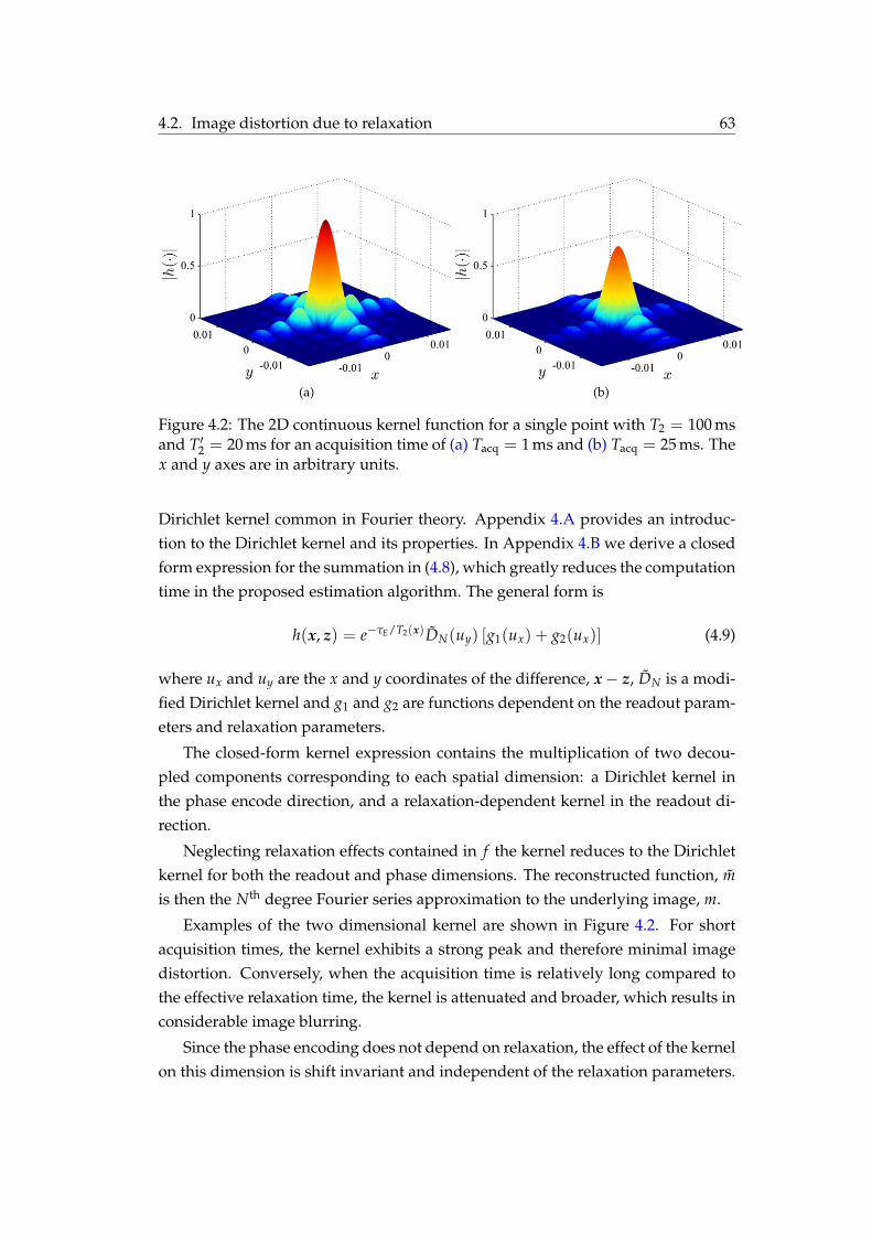
4.2. Image distortion due to relaxation 63
(a) (b)
Figure 4.2: The 2D continuous kernel function for a single point with T2 = 100 msand T′2 = 20 ms for an acquisition time of (a)(a) Tacq = 1 ms and (b)(b) Tacq = 25 ms. Thex and y axes are in arbitrary units.
Dirichlet kernel common in Fourier theory. Appendix 4.A4.A provides an introduc-tion to the Dirichlet kernel and its properties. In Appendix 4.B4.B we derive a closedform expression for the summation in (4.84.8), which greatly reduces the computationtime in the proposed estimation algorithm. The general form is
h(x, z) = e−τE/T2(x)DN(uy) [g1(ux) + g2(ux)] (4.9)
where ux and uy are the x and y coordinates of the difference, x− z, DN is a modi-fied Dirichlet kernel and g1 and g2 are functions dependent on the readout param-eters and relaxation parameters.
The closed-form kernel expression contains the multiplication of two decou-pled components corresponding to each spatial dimension: a Dirichlet kernel inthe phase encode direction, and a relaxation-dependent kernel in the readout di-rection.
Neglecting relaxation effects contained in f the kernel reduces to the Dirichletkernel for both the readout and phase dimensions. The reconstructed function, mis then the Nth degree Fourier series approximation to the underlying image, m.
Examples of the two dimensional kernel are shown in Figure 4.24.2. For shortacquisition times, the kernel exhibits a strong peak and therefore minimal imagedistortion. Conversely, when the acquisition time is relatively long compared tothe effective relaxation time, the kernel is attenuated and broader, which results inconsiderable image blurring.
Since the phase encoding does not depend on relaxation, the effect of the kernelon this dimension is shift invariant and independent of the relaxation parameters.

64 Chapter 4. Estimation of relaxation rates in the presence of image distortion
0
0.2
0.4
0.6
0.8
1
Position (m)
Slice
of|h(x,z)|
−
3LN
−
2LN
−
LN
0 LN
2LN
3LN
Tacq = 1msTacq = 5msTacq = 10msTacq = 15ms
(a)
0
0.2
0.4
0.6
0.8
1
0 NL
Spatial frequency (rad/m)
|H(k)|
Tacq = 1msTacq = 5msTacq = 10msTacq = 15ms
(b)
Figure 4.3: Analysis of the filter kernel for different acquisition times displaying(a)(a) the continuous filter kernel and (b)(b) the corresponding frequency response. Aslice along the readout direction is displayed for T2 = 100 ms and T′2 = 20 ms.
The filter in this direction is a Dirichlet kernel and its effect is well characterised byFourier theory. Conversely the filter kernel along the readout direction is depen-dent on relaxation and creates an additional distortion. The purpose of this sectionis to investigate such a distortion. It is therefore constructive to focus our analysison a 1D slice of the kernel along the readout direction.
We analyse the full kernel expression from a filtering perspective by calculatingthe frequency response of the windowed kernel at a location with T2 = 100 msand T′2 = 20 ms for different sampling rates. Figure 4.34.3 presents the spatial kerneland the corresponding frequency response for different acquisition times. The lowpass nature of the filter is clear whereby the high frequency content is increasinglyattenuated for larger acquisition times. In the spatial domain, attenuation of highfrequencies corresponds to image blurring.
We investigate the low-pass characteristics of the filter by simulating the ac-quisition and reconstruction of a Shepp-Logan numerical phantom [6060]. As theacquisition and sampling time decrease, f (k, x) → e−τE/T2(x), and the image is aweighted M0(·) as in (4.134.13). The effect of a non-zero sampling interval on recon-structed images is investigated in the Figure 4.44.4. To quantify the level of distortion,the mean square error (MSE) between the output image and the true image is plot-ted for different acquisition times as shown in Figure 4.54.5.

4.2. Image distortion due to relaxation 65
(a) Weighted image (b) Tacq = 5ms (c) Tacq = 15ms (d) Tacq = 25ms
Figure 4.4: Reconstructed images (top) and a region-of-interest (bottom) from sim-ulated data using the linear filter model for increasing acquisition times. For longacquisition times considerable image blurring is present.
0 5 10 15 20 25
0
0.2
0.4
0.6
0.8
1
1.2
Echo sampling time (ms)
MSE
(×10
−4)
Figure 4.5: The mean squared error (MSE) of a reconstructed phantom as a func-tion of acquisition time.

66 Chapter 4. Estimation of relaxation rates in the presence of image distortion
4.2.2 Filter kernel approximation
A simple approximation to the kernel function is obtained by introducing two as-sumptions:
A4.1 No relaxation occurs during the sampling of the observations, s(k). This isvalid for Tacq much smaller than the effective decay time. In this case t ≈ τE
and only the peak of the echo is sampled or in terms of the filter kernel,f (k(t), x) ≈ f (k(τE), x).
A4.2 The number of measurements is large such that the Dirichlet kernel approachesa delta function, DN(x) ≈ δ(x).
For spin echo, these two assumptions result in a kernel
h(x, z) = e−τE/T2(z)δ(x− z) (4.10)
Substituting this into the signal model gives,
m(z) =∫
m(x)h(x, z)dx (4.11)
=∫
m(x)e−τE/T2(x)δ(x− z)dx (4.12)
= m(z)e−τE/T2(z) (4.13)
Therefore, with this approximation we reconstruct a spatially weighted versionof the initial magnetisation.
4.3 Measurement model for relaxation time estimation
A reasonable assumption for biological tissues (where T1 > T2) using acquisi-tion sequences with long repetition times, is that the effect of T1 relaxation isnegligible. The unknown parameters depend on the specific imaging paradigm.For spin echo sequences the relevant parameters at the pth object position areθp = [T2(xp), T′2(xp), M0(xp)]T where xp is a point on a Nx × Ny grid over theobject. The vector of all important parameters is
θ = [θT1 , . . . , θT
N ]T, N = Nx × Ny. (4.14)
Estimation of the relaxation parameters is performed by first acquiring a se-quence of M images at different echo times. As discussed in Chapter 33 the CPMG

4.3. Measurement model for relaxation time estimation 67
sequence generates multiple echoes from a single excitation, which allows suchdata to be collected efficiently.
We wish to consider inversion of the signal model in (4.74.7). For this purpose itis useful to approximate the underlying signal by a sum of delta functions,
m(x) ≈∑p
m(xp)δ(x− xp) (4.15)
We also recognise that the DFT used for image reconstruction produces discretesamples of the function, m(·), on the reconstruction grid, z1 . . . , zN . The signalmodel now becomes
m(zr) = ∑p
m(xp)h(xp, zr) (4.16)
The combination of the DFT and basis decomposition of the underlying signalleads to a sampling of the continuous kernel, h(·, ·), at the Fourier frequencies.
We denote the k-space observations corresponding to the nth echo as sn(ki)
where ki is a grid point in 2-D k-space. The measurements can be expressed as,
sn(ki) =N
∑p=1
m(xp) f nθ (ki, xp)ejki ·xp + vn,i. (4.17)
The sequence vn,i is white complex Gaussian noise with variance σ2 and f nθ (k, x)
is the relaxation function, representing the acquisition and relaxation components.
As described in Section 4.24.2, these observations are collected in 2D frequencyspace and distortions occur in image space due to relaxation. We approximatethe integral in (4.14.1) by a summation over the grid used for the parameter vector.Other modifications here are the superscript n denoting the image index and thenotation f n
θ to acknowledge the dependence of the unknown parameters on theimaging kernel. The additive noise has also been explicitly included highlightingthe stochastic nature of the measurements.
The relaxation function takes the form of (4.24.2) with the echo time now depen-dent on the image index, n. Specifically,
f nθ (ki, x) = e−τn/T2(x)e−|ti−τn|/T′2(x) (4.18)
where τn is the echo time and ti is the time after excitation. Figure 4.64.6 shows theacquisition parameters and signal amplitude for a spin echo sequence.
The standard method used to reconstruct the image, mn, is the inverse discrete

68 Chapter 4. Estimation of relaxation rates in the presence of image distortion
0
0.2
0.4
0.6
0.8
1
Effective decay e− t/T ∗
2 where 1T ∗
2= 1
T2+ 1
T ′
2
...
τ1 τ2 τ3
SignalAmplitu
de(×
M0)
T ime, t
Ta c q
T2 Decay e− t/T2
Figure 4.6: Signal amplitude of the bulk magnetisation during data acquisition fora spin echo sequence.
Fourier transform:
mn(zr) =N
∑p=1
m(xp)hnθ(xp, zr) + en,r (4.19)
where zr is a grid point in the output image, and the filter kernel, hnθ(x, z), is de-
fined as
hnθ(x, z) =
N
∑i=1
f nθ (ki, x)ejki ·(x−z). (4.20)
The noise in image domain, en,r, is approximately white complex Gaussian fora sufficiently large N. A closed form for (4.204.20) has been found to simplify cal-culations. In this framework, the reconstructed image is interpreted as a filteredversion of the initial magnetisation, M0(x), with the linear space-varying filter de-fined by the kernel, hn
θ(x, z). This kernel models the spatial distortion in an imageand provides an opportunity to reverse such distortion. Importantly, the kernelis dependent on both the acquisition parameters, (T, Tacq, τn), and the unknownrelaxation parameters, θ. The properties of this kernel and its effect on relaxationtime estimation are examined in detail in subsequent sections of this chapter.
Let yn,r = mn(zr) and denote yn = [yn,1, . . . , yn,N ]T. The observations from
each echo image form a complete measurement vector, y = [yT1 , . . . yT
M]T. Themeasurements are complex, y ∈ CNM, and the parameters are positive and real,θ ∈ [0, ∞)2N . The goal is to find an estimator for T∗2 and as such, M0 is a nuisanceparameter so we find an estimator θ : CNM 7→ [0, ∞)2N .
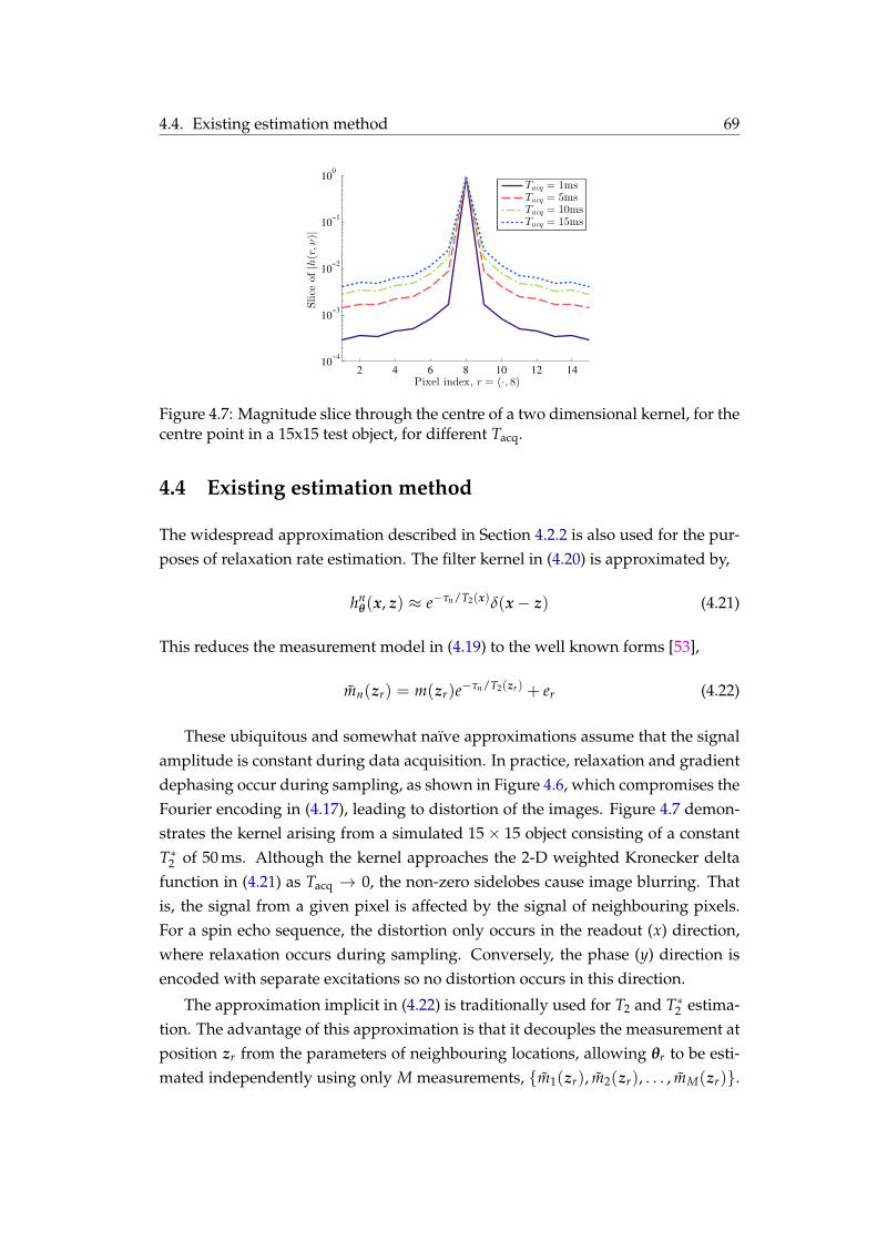
4.4. Existing estimation method 69
2 4 6 8 10 12 1410
−4
10−3
10−2
10−1
100
Pixel index, r = (·, 8)
Slice
of|h(r,ν)|
Tacq = 1msTacq = 5msTacq = 10msTacq = 15ms
Figure 4.7: Magnitude slice through the centre of a two dimensional kernel, for thecentre point in a 15x15 test object, for different Tacq.
4.4 Existing estimation method
The widespread approximation described in Section 4.2.24.2.2 is also used for the pur-poses of relaxation rate estimation. The filter kernel in (4.204.20) is approximated by,
hnθ(x, z) ≈ e−τn/T2(x)δ(x− z) (4.21)
This reduces the measurement model in (4.194.19) to the well known forms [5353],
mn(zr) = m(zr)e−τn/T2(zr) + er (4.22)
These ubiquitous and somewhat naïve approximations assume that the signalamplitude is constant during data acquisition. In practice, relaxation and gradientdephasing occur during sampling, as shown in Figure 4.64.6, which compromises theFourier encoding in (4.174.17), leading to distortion of the images. Figure 4.74.7 demon-strates the kernel arising from a simulated 15× 15 object consisting of a constantT∗2 of 50 ms. Although the kernel approaches the 2-D weighted Kronecker deltafunction in (4.214.21) as Tacq → 0, the non-zero sidelobes cause image blurring. Thatis, the signal from a given pixel is affected by the signal of neighbouring pixels.For a spin echo sequence, the distortion only occurs in the readout (x) direction,where relaxation occurs during sampling. Conversely, the phase (y) direction isencoded with separate excitations so no distortion occurs in this direction.
The approximation implicit in (4.224.22) is traditionally used for T2 and T∗2 estima-tion. The advantage of this approximation is that it decouples the measurement atposition zr from the parameters of neighbouring locations, allowing θr to be esti-mated independently using only M measurements, m1(zr), m2(zr), . . . , mM(zr).
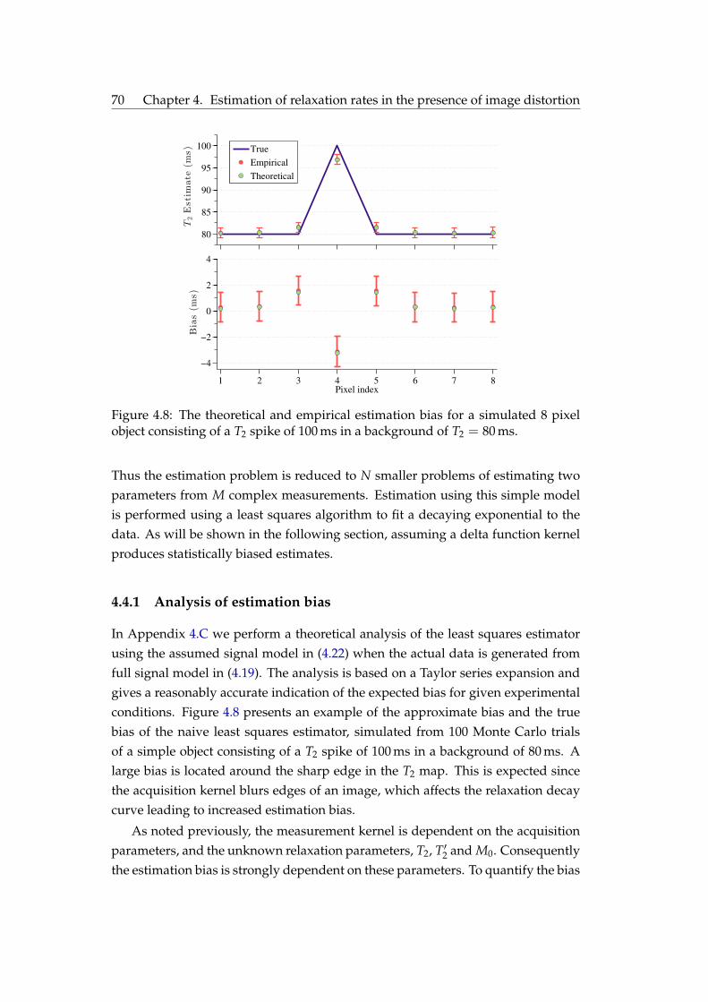
70 Chapter 4. Estimation of relaxation rates in the presence of image distortion
80
85
90
95
100
T2Estimate
(ms)
True
Empirical
Theoretical
1 2 3 4 5 6 7 8
−4
−2
0
2
4
Bias(m
s)
Pixel index
Figure 4.8: The theoretical and empirical estimation bias for a simulated 8 pixelobject consisting of a T2 spike of 100 ms in a background of T2 = 80 ms.
Thus the estimation problem is reduced to N smaller problems of estimating twoparameters from M complex measurements. Estimation using this simple modelis performed using a least squares algorithm to fit a decaying exponential to thedata. As will be shown in the following section, assuming a delta function kernelproduces statistically biased estimates.
4.4.1 Analysis of estimation bias
In Appendix 4.C4.C we perform a theoretical analysis of the least squares estimatorusing the assumed signal model in (4.224.22) when the actual data is generated fromfull signal model in (4.194.19). The analysis is based on a Taylor series expansion andgives a reasonably accurate indication of the expected bias for given experimentalconditions. Figure 4.84.8 presents an example of the approximate bias and the truebias of the naive least squares estimator, simulated from 100 Monte Carlo trialsof a simple object consisting of a T2 spike of 100 ms in a background of 80 ms. Alarge bias is located around the sharp edge in the T2 map. This is expected sincethe acquisition kernel blurs edges of an image, which affects the relaxation decaycurve leading to increased estimation bias.
As noted previously, the measurement kernel is dependent on the acquisitionparameters, and the unknown relaxation parameters, T2, T′2 and M0. Consequentlythe estimation bias is strongly dependent on these parameters. To quantify the bias

4.5. Proposed estimation method 71
T∗
2 (ms)
Tacq(m
s)
1 2 3 4 5 6 7 8 9 10
1
2
3
4
5
6
7
8
9
10
0
2
4
6
8
10
12
14
16
18
20
(%)
(a)T
∗
2 (ms)
Tacq(m
s)
1 2 3 4 5 6 7 8 9 10
1
2
3
4
5
6
7
8
9
10
0
2
4
6
8
10
12
14
16
18
20
(%)
(b)
Figure 4.9: Estimation bias generated from (a)(a) theoretical analysis and (b)(b) 100Monte Carlo trials as a function of the acquisition time Tacq and the effective re-laxation time T∗2 . The simulated 8 pixel object consists of a T2 spike of 100 ms in abackground of T2 = 80 ms.
over a range of situations, we repeat the experiment above for different pairs ofTacq and T∗2 . For each set of parameters we calculate the approximate bias and theempirical bias from 1000 Monte Carlo trials. Figure 4.94.9 shows the resultant bias asa function of Tacq and T∗2 and demonstrates the close match between our analyticalbias and the true bias over a broad range of parameters. Note that some regionsof the aggregate parameter space show near zero bias whereas other regions showsignificant bias. The regions with minimal bias are when Tacq T∗2 , validatingthe assumption made in (4.224.22). However, it will be shown in the next section, that,improved estimates are achievable by acquiring samples with increased SNR andaccounting for the image distortion.
4.5 Proposed estimation method
We propose estimation of relaxation times using the full measurement model in(4.194.19). In contrast to the pixel-independent estimation problems using (4.224.22), inthis case, all the parameters, θ, must be estimated jointly. The joint estimationproblem is substantially more difficult due to the large number of parameters anda simple non-linear least squares algorithm performs poorly and struggles to con-verge to the global minimum. Thus, we propose a Bayesian estimation algorithm.

72 Chapter 4. Estimation of relaxation rates in the presence of image distortion
4.5.1 Algorithm
In Bayesian estimation we aim to find the posterior probability density, π(θ|y).With this density, the minimum mean-squared-error estimate, θ, can be obtainedby evaluating the conditional expectation, θ = Eπ[θ|y]. We cannot compute thisexpectation in closed form so we use Monte Carlo samples from π(θ|y). The prob-lem setup lends itself to a Gibbs sampler [6161] for drawing the posterior samples.A Gibbs sampler is a Markov chain constructed by drawing from conditional dis-tributions such that its invariant distribution is π(θ|y) [6262]. The conditional distri-butions have the form π(θj|θ[¬j], y) where θ[¬j] are the elements in θ excluding thejth element. Bayes’ rules states that
π(θj|y, θ[¬j]) ∝ `(y|θj, θ[¬j])π0(θj|θ[¬j]). (4.23)
We adopt a Gaussian prior for π0(θj|θ[¬j]) defined by π0(θ) = N (θ; θ, Λ), whereθ is the least squares estimate and Λ is a diagonal covariance matrix. In this work,we define Λ with variances of 502 ms for the relaxation times and 0.42 for the initialmagnetisation, noting that the naive least squares estimator will provide a reason-able initial estimate. The signal model in (4.194.19) defines the expected signal as
µn,r(θ) =N
∑p=1
m(xp)hnθ(xp, zr). (4.24)
For µ(θ) = [µ1,1(θ), µ1,2(θ), . . . , µM,N(θ)]T, the likelihood is
`(y|θj, θ[¬j]) = N (y; µ(θj; θ[¬j]), Σ) (4.25)
We assume the measurement noise is white Gaussian and independent, thus Σ =
diag(σ2, . . . , σ2).To draw samples, we approximate π(θj|y, θ[¬j]) by a piecewise uniform dis-
tribution [6363], constructed by evaluating the posterior on an adaptive set of gridpoints, ζ1, . . . , ζG, to obtain weights w1, . . . , wG. Each grid point, ζi, defines a uni-form distribution on the interval [ζi−∆G/2, ζi +∆G/2], denoted U[ζi−∆G/2,ζi+∆G/2],creating a piece-wise continuous distribution across the grid. The grid is adaptivesince it is redefined every iteration. The first point of the grid is chosen to be thecurrent estimate and successive grid points are added in each direction until thecalculated weights are close to zero. Furthermore, the grid spacing, ∆G, is adjustedfrom one iteration to the next to keep the grid size close to a nominal value, de-noted G0.
The algorithm is run for P iterations and samples are collected after P0 itera-

4.5. Proposed estimation method 73
tions to allow the Markov chain to converge [6464]. These samples, θ(t), t = P0, . . . , P,are used to calculate the point estimate, θ = 1
P−P0∑P
t=P0θ(t). The complete algo-
rithm is listed in Algorithm 4.14.1.
Algorithm 4.1: Bayesian Estimation AlgorithmInput: y – observationsOutput: θ – estimateParams: Σ – noise covariance, Λ – prior covariance, P – number of samples,
P0 – Markov chain “burn in”, G0 – desired grid size, ∆0 – initial gridspacing
1 Calculate least squares estimates θ1, . . . , θN .2 θ← [θ1, . . . , θN ]3 ∆G ← ∆04 for t← 1, . . . , P do5 for j← 1, . . . , 2N do6 Set k← 1, ζk ← θj
7 Set wmax = 08 repeat9 Compose: ϑ ← [ζk, θ[¬j]]
10 Calculate: µ(ϑ) from (4.244.24)11 Calculate: wk ← N (y; µ(ϑ), Λ)π0(ζk|θ[¬j])
12 Assign: wmax ← wk if wk > wmax13 Pick next grid point, ζk+1; k← k + 114 until wk < 0.01wmax15 Normalise weights: wk ← wk/ ∑i wi
16 Sample θ(t)j ∼ ∑
gk=1 wkU[ζk−∆/2,ζk+∆/2]
17 Adjust grid spacing, ∆G ← (1 + (G− G0)/G0)∆G
18 Return estimate: θ← 1P−P0
∑Pt=P0
θ(t)
4.5.2 Properties of the Bayesian estimation algorithm
As explained in Section 3.7.13.7.1, the noise variance, σ2, in an MRI experiment is pro-portional to the receiver bandwidth, BW = 1/Tacq. The signal-to-noise ratio of theimaging system is defined as SNR = s/σ where s is the signal amplitude, whichwe assume to be constant. Thus
SNR ∝√
Tacq. (4.26)
As Figure 4.94.9 illustrates, in many practical cases the distortion introduced bythe finite sampling bandwidth (or non-zero acquisition time) is negligible. How-ever, even in these cases, it is possible to obtain a smaller estimation error by se-

74 Chapter 4. Estimation of relaxation rates in the presence of image distortion
10
15
20
25
R2(s
−1 )
True
1 2 3 4 5 6 7 8
10−8
10−6
10−4
Pixel Index
MSE
Naive Estimator
Proposed
Figure 4.10: Comparison of the proposed T2 estimation algorithm and the naïveleast-squares approach showing the true R2 = 1/T2 profile and the mean squareerror for both approaches calculated from 100 noise realisations.
lecting a longer acquisition time and using the proposed estimator to account forthe increased distortion. The increase in Tacq improves the SNR which decreasesthe estimation variance.
4.6 Simulations
The estimation algorithm developed in the previous sections is demonstrated us-ing a CPMG sequence with multiple echoes. We simulate the spin echo sequencewith echo times defined by τn = (4.5 + 3.5(n− 1))ms for n = 1, . . . , M. We useM = 16, and a relatively long Tacq = 5.12 ms, for a numerical object defined in Fig-ure 4.104.10, with T2 features typical of a human brain [6565] and M0 = 1 representing aconstant proton density. The naïve estimator using non-linear least squares on thesimple measurement model in (4.224.22) is compared with the proposed algorithm us-ing the complete model in (4.194.19). The algorithm was run using P = 1100, P0 = 100,Λ = diag(2.5× 10⁻⁵, 10−2, . . . , 2.5× 10⁻⁵, 10−2). The estimation was repeated for100 realisations of noise.
The results are shown in Figure 4.104.10 where the rate, R2 = 1/T2 is displayedfollowing the convention in MRI literature. The Bayesian algorithm has a smallermean-square-error and successfully compensates for the distortion. Figure 4.114.11demonstrates that the estimation error can always be decreased by increasing Tacq
and reaping the benefits of improved SNR whilst counteracting the increase indistortion using the proposed estimator. Conversely, the performance of any algo-rithm that fails to account for the distortion, will degrade as Tacq increases.

4.7. Discussion and conclusion 75
0 1 2 3 4 5
10−7
10−6
10−5
10−4
10−3
Tacq (ms)
MSE
Naive EstimatorProposed
Figure 4.11: Mean square error, as Tacq increases, of the proposed algorithm andthe naïve least-squared estimator. The simulation setup is otherwise the same asused for Figure 4.104.10.
An important implication of these results is revealed by considering the SNRdependencies discussed in Section 3.7.13.7.1. The SNR increases linearly with fieldstrength and the MSE decreases with increasing SNR. Consequently, the same levelof accuracy of current systems can be achieved with a much weaker field strengthand an improved signal model.
Figure 4.124.12 displays the bias and variance of both estimators. This highlightsthat although the variance of the naive estimator deceases with increased SNR dueto longer Tacq, the bias is the dominant source of error. Thus for the naive estimator,the potential improvement from increased SNR is outweighed by the increase inestimation bias.
4.7 Discussion and conclusion
In this chapter, the image distortion introduced by signal relaxation during sam-pling was investigated and modelled with a linear filter. The filter kernel wasexamined in detail, both analytically and through simulation. In the context ofMRI relaxation rate estimation, it was revealed that this distortion leads to statisti-cal bias when the commonly accepted signal model is used. Due to the acquisitionnoise properties, such estimators incur a tradeoff between bias and SNR. We havepresented an algorithm suitable to estimate the transverse relaxation rate from spinecho sequences. The proposed estimator overcomes this tradeoff by accounting forthe distortion in reconstructed images, resulting in improved estimates.
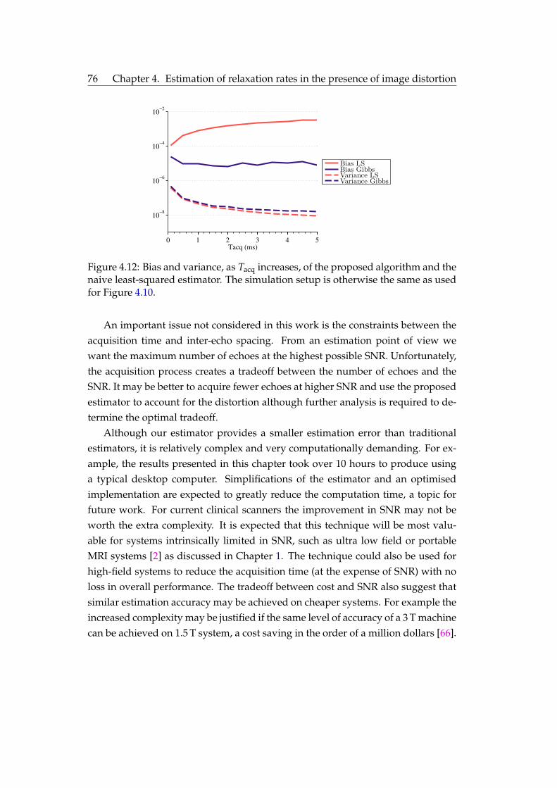
76 Chapter 4. Estimation of relaxation rates in the presence of image distortion
0 1 2 3 4 5
10−8
10−6
10−4
10−2
Tacq (ms)
Bias LSBias GibbsVariance LSVariance Gibbs
Figure 4.12: Bias and variance, as Tacq increases, of the proposed algorithm and thenaive least-squared estimator. The simulation setup is otherwise the same as usedfor Figure 4.104.10.
An important issue not considered in this work is the constraints between theacquisition time and inter-echo spacing. From an estimation point of view wewant the maximum number of echoes at the highest possible SNR. Unfortunately,the acquisition process creates a tradeoff between the number of echoes and theSNR. It may be better to acquire fewer echoes at higher SNR and use the proposedestimator to account for the distortion although further analysis is required to de-termine the optimal tradeoff.
Although our estimator provides a smaller estimation error than traditionalestimators, it is relatively complex and very computationally demanding. For ex-ample, the results presented in this chapter took over 10 hours to produce usinga typical desktop computer. Simplifications of the estimator and an optimisedimplementation are expected to greatly reduce the computation time, a topic forfuture work. For current clinical scanners the improvement in SNR may not beworth the extra complexity. It is expected that this technique will be most valu-able for systems intrinsically limited in SNR, such as ultra low field or portableMRI systems [22] as discussed in Chapter 11. The technique could also be used forhigh-field systems to reduce the acquisition time (at the expense of SNR) with noloss in overall performance. The tradeoff between cost and SNR also suggest thatsimilar estimation accuracy may be achieved on cheaper systems. For example theincreased complexity may be justified if the same level of accuracy of a 3 T machinecan be achieved on 1.5 T system, a cost saving in the order of a million dollars [6666].

4.A. Introduction to the Dirichlet kernel 77
Appendices
4.A Introduction to the Dirichlet kernel
The Dirichlet kernel is defined as
DN(x) :=
N−12
∑k=− N−1
2
ejkx. (4.27)
which assumes symmetric sampling of k. That is, N is odd and k is summed from−N−1
2 to N−12 . In reality, traditional use of the Fast Fourier Transform (FFT) favours
an even number of samples. Furthermore, it is desirable to sample the point k = 0and thus, as pointed out in [5353, Page 240], MRI samples are typically collected fromsampling from −N
2 to N2 − 1 for even N. In this case we have the relationship,
DN(x) = DN−1(x) + e−jN/2x (4.28)
This subtle discrepancy in the definition does not effect the general behaviour ofthe function; it merely adds a linear phase term, consistent our understanding ofthe Fourier sampling in MRI. Fig. 4.134.13 demonstrates the behaviour of DN(x) forincreasing number of measurements. We see that the period is 2π regardless of thenumber of measurements and as N → ∞, the Dirichlet kernel approaches a Diraccomb. For application in MRI, the period of the Dirichlet kernel is modified byscaling the argument by the sampling properties. In (7.417.41), the argument is scaledby Rx∆xWx when x = (nWx, mWy).
−10 −5 0 5 10
−20
0
20
40
60
80
x
DirichletKernel,D
N(x)
N = 64N = 32N = 16
(a)
−0.4 −0.2 0 0.2 0.4 0.6
−20
0
20
40
60
80
x
DirichletKernel,D
N(x)
N = 64N = 32N = 16
(b)
Figure 4.13: The Dirichlet kernel for three measurement sample sizes. (a) demon-strates the fixed period of the kernel while (b) indicates that the kernel approachesa Dirac comb for N → ∞.
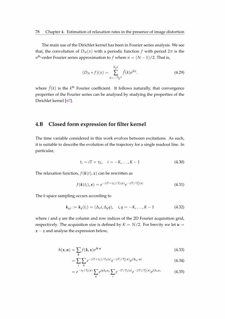
78 Chapter 4. Estimation of relaxation rates in the presence of image distortion
The main use of the Dirichlet kernel has been in Fourier series analysis. We seethat, the convolution of DN(x) with a periodic function f with period 2π is thenth-order Fourier series approximation to f where n = (N − 1)/2. That is,
(DN ∗ f )(x) =N−1
2
∑k=− N−1
2
f (k)ejkx. (4.29)
where f (k) is the kth Fourier coefficient. It follows naturally, that convergenceproperties of the Fourier series can be analysed by studying the properties of theDirichlet kernel [6767].
4.B Closed form expression for filter kernel
The time variable considered in this work evolves between excitations. As such,it is suitable to describe the evolution of the trajectory for a single readout line. Inparticular,
ti = iT + τE, i = −K, . . . , K− 1 (4.30)
The relaxation function, f (k(t), x) can be rewritten as
f (k(ti), x) = e−(iT+τE)/T2(x)e−|iT|/T′2(x) (4.31)
The k-space sampling occurs according to
kq,i := kq(ti) = (∆xi, ∆yq), i, q = −K, . . . , K− 1 (4.32)
where i and q are the column and row indices of the 2D Fourier acquisition grid,respectively. The acquisition size is defined by K = N/2. For brevity we let u =
x− z and analyse the expression below,
h(x, u) = ∑k
f (k, x)ejk·u (4.33)
= ∑i
∑q
e−(iT+τE)/T2(x)e−|iT|/T′2(x)ej(kq,i ·u) (4.34)
= e−τE/T2(x) ∑q
ejq∆yuy ∑i
e−iT/T2(x)e−|iT|/T′2(x)eji∆xux (4.35)
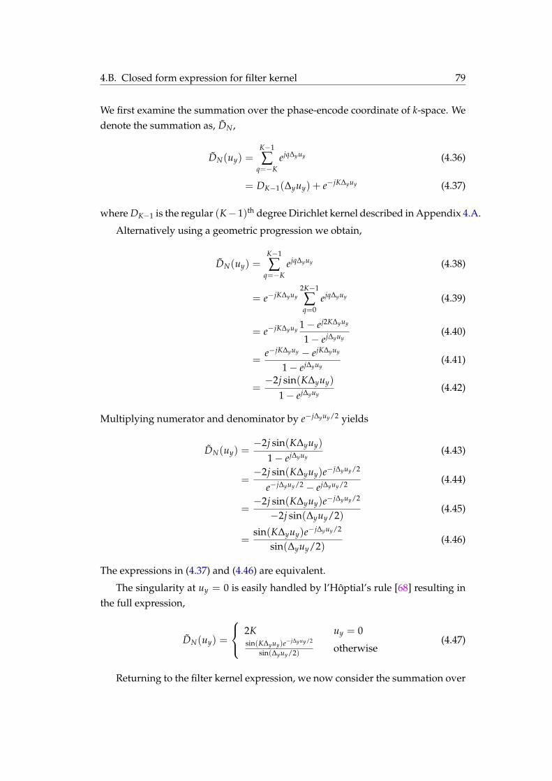
4.B. Closed form expression for filter kernel 79
We first examine the summation over the phase-encode coordinate of k-space. Wedenote the summation as, DN ,
DN(uy) =K−1
∑q=−K
ejq∆yuy (4.36)
= DK−1(∆yuy) + e−jK∆yuy (4.37)
where DK−1 is the regular (K− 1)th degree Dirichlet kernel described in Appendix 4.A4.A.
Alternatively using a geometric progression we obtain,
DN(uy) =K−1
∑q=−K
ejq∆yuy (4.38)
= e−jK∆yuy2K−1
∑q=0
ejq∆yuy (4.39)
= e−jK∆yuy1− ej2K∆yuy
1− ej∆yuy(4.40)
=e−jK∆yuy − ejK∆yuy
1− ej∆yuy(4.41)
=−2j sin(K∆yuy)
1− ej∆yuy(4.42)
Multiplying numerator and denominator by e−j∆yuy/2 yields
DN(uy) =−2j sin(K∆yuy)
1− ej∆yuy(4.43)
=−2j sin(K∆yuy)e−j∆yuy/2
e−j∆yuy/2 − ej∆yuy/2 (4.44)
=−2j sin(K∆yuy)e−j∆yuy/2
−2j sin(∆yuy/2)(4.45)
=sin(K∆yuy)e−j∆yuy/2
sin(∆yuy/2)(4.46)
The expressions in (4.374.37) and (4.464.46) are equivalent.
The singularity at uy = 0 is easily handled by l’Hôptial’s rule [6868] resulting inthe full expression,
DN(uy) =
2K uy = 0sin(K∆yuy)e−j∆yuy/2
sin(∆yuy/2) otherwise(4.47)
Returning to the filter kernel expression, we now consider the summation over

80 Chapter 4. Estimation of relaxation rates in the presence of image distortion
the readout coordinate,
g(ux) =K−1
∑i=−K
e−iT/T2(x)e−|iT|/T′2(x)eji∆xux (4.48)
=−1
∑i=−K
e−iT/T2(x)eiT/T′2(x)eji∆xux +K−1
∑i=0
e−iT/T2(x)e−iT/T′2(x)eji∆xux (4.49)
Now define
1T∗2 (x)
=1
T2(x)+
1T′2(x)
(4.50)
1T−2 (x)
=1
T2(x)− 1
T′2(x)(4.51)
such that g(ux) can be written as
g(ux) =−1
∑i=−K
e−iT/T−2 (x)eji∆xux +K−1
∑i=0
e−iT/T∗2 (x)eji∆xux (4.52)
Consider the first term, which we denote g1,
g1(ux) =−1
∑i=−K
ei(−T/T−2 (x)+j∆xux) (4.53)
= e−K(−T/T−2 (x)+j∆xux)K−1
∑i=0
ei(−T/T−2 (x)+j∆xux) (4.54)
= e−K(−T/T−2 (x)+j∆xux) 1− eK(−T/T−2 (x)+j∆xux)
1− e(−T/T−2 (x)+j∆xux)(4.55)
=−1 + e−K(−T/T−2 (x)+j∆xux)
1− e(−T/T−2 (x)+j∆xux)(4.56)
Similarly for the second term, g2, we get
g2(ux) =K−1
∑i=0
ei(−T/T∗2 (x)+j∆xux) (4.57)
=1− eK(−T/T∗2 (x)+j∆xux)
1− e(−T/T∗2 (x)+j∆xux)(4.58)
We can now write the expression for the filter kernel that does not involve anysummations. That is,
h(x, z) = e−τE/T2(x)DN(uy) [g1(ux) + g2(ux)] (4.59)

4.C. Analysis of estimation bias 81
where ux and uy are the x and y coordinates of the difference, x− z.
4.C Analysis of estimation bias
The least squares estimator minimises the following cost function
f (θ) =M
∑i=1
(yi − gi(θ))2 (4.60)
where gi = me−ti/T2 .
The derivative of the cost function at the least squares estimate will be zero.That is,
J(θ) = ∇θ f (θ)|θ=θ = 0 (4.61)
where∇θ = [∂/∂m, ∂/∂T2]T. Taking the first order Taylor series expansion aroundthe true parameter θ? yields
J(θ) = 0 ≈ J(θ?) + H(θ?)(θ− θ?) (4.62)
where H(θ) = ∇θ∇Tθ f (θ)|θ=θ. The bias is then approximated by
bias = E[θ− θ?
]≈ −E
[H−1(θ?)J(θ?)
](4.63)
In our case,
J(θ) =[
∂ f∂M
∂ f∂T
]T(4.64)
H(θ) =
[∂2 f∂M2
∂2 f∂MT
∂2 f∂TM
∂2 f∂T2
](4.65)
For the sake of brevity we let f ′T = ∂ f∂T , f ′M = ∂ f
∂M , f ′TT = ∂2 f∂T2 , f ′MM = ∂ f
∂M2 ,f ′TM = ∂ f
∂TM . The inverse of the 2× 2 matrix H can be computed explicitly as
H−1(θ) =1
f ′TT(θ) f ′MM(θ)− f ′TM(θ) f ′MT(θ)
[f ′TT(θ) − f ′TM(θ)
− f ′MT(θ) f ′MM(θ)
](4.66)
The relevant derivatives are
f ′V(θ) = −2M
∑i=1
(yi − gi(θ))g′i,V(θ) (4.67)

82 Chapter 4. Estimation of relaxation rates in the presence of image distortion
= −2M
∑i=1
(µt(θ?)− gi(θ))g′i,V(θ)− 2
M
∑i=1
vig′i,V(θ) (4.68)
and
f ′VW(θ) = −2M
∑i=1
[(yi − gi(θ))g′′i,VW(θ)− g′i,W(θ)g′i,V(θ)
](4.69)
= −2M
∑i=1
[(µt(θ
?)− gi(θ))g′′i,VW(θ)− g′i,W(θ)g′i,V(θ)]− 2
M
∑i=1
vig′′i,VW(θ)
(4.70)
where V and W can be different combinations of the variables T and M. The indi-vidual derivatives of g(θ) are
gi(θ) = me−ti/T2 (4.71)
g′i,T(θ) =mti
T22
e−ti/T2 (4.72)
g′i,M(θ) = e−ti/T2 (4.73)
The second derivatives are
g′′i,TT(θ) =−2mti
T32
e−ti/T2 +mt2
i
T42
e−ti/T2 (4.74)
g′′i,MM(θ) = 0 (4.75)
g′′i,TM(θ) = g′′i,MT(θ) =ti
T22
e−ti/T2 (4.76)
The two elements of the matrix multiplication in (4.634.63) are obtained by
biasM = E
[f ′M(θ) f ′TT(θ)− fT(θ) f ′TM(θ)
f ′TT(θ) f ′MM(θ)− f ′TM(θ) f ′MT(θ)
](4.77)
biasT = E
[fT(θ) f ′MM(θ)− fM(θ) f ′MT(θ)
f ′TT(θ) f ′MM(θ)− f ′TM(θ) f ′MT(θ)
](4.78)
Each f ′ factor above is a scalar that can be written in the form αT β + ξv, where α,β, and ξ are deterministic and v is the stochastic noise. Multiplication of two suchfactors gives a quadratic form in v. The desired bias is given by the expectation ofthe ratio of two such forms. The relevant expectation can be written as
E[η
δ
]= E
[a + bTv + vT Avc + dTv + vTBv
](4.79)
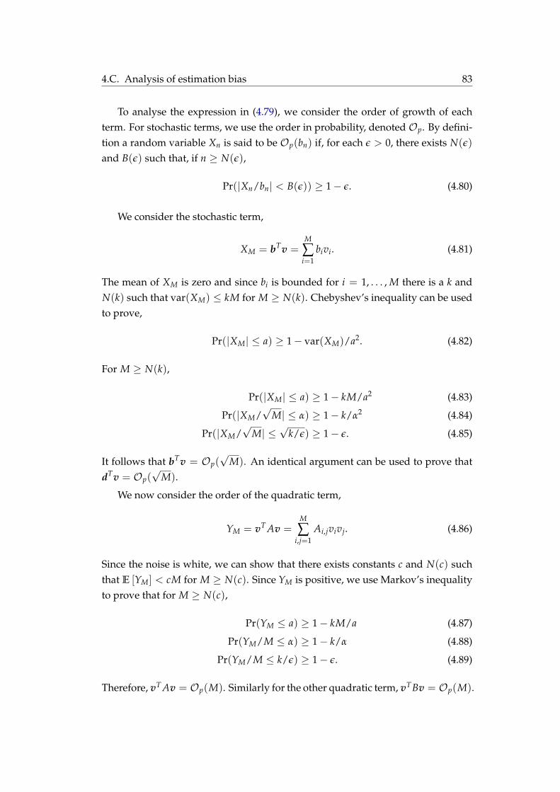
4.C. Analysis of estimation bias 83
To analyse the expression in (4.794.79), we consider the order of growth of eachterm. For stochastic terms, we use the order in probability, denoted Op. By defini-tion a random variable Xn is said to be Op(bn) if, for each ε > 0, there exists N(ε)
and B(ε) such that, if n ≥ N(ε),
Pr(|Xn/bn| < B(ε)) ≥ 1− ε. (4.80)
We consider the stochastic term,
XM = bTv =M
∑i=1
bivi. (4.81)
The mean of XM is zero and since bi is bounded for i = 1, . . . , M there is a k andN(k) such that var(XM) ≤ kM for M ≥ N(k). Chebyshev’s inequality can be usedto prove,
Pr(|XM| ≤ a) ≥ 1− var(XM)/a2. (4.82)
For M ≥ N(k),
Pr(|XM| ≤ a) ≥ 1− kM/a2 (4.83)
Pr(|XM/√
M| ≤ α) ≥ 1− k/α2 (4.84)
Pr(|XM/√
M| ≤√
k/ε) ≥ 1− ε. (4.85)
It follows that bTv = Op(√
M). An identical argument can be used to prove thatdTv = Op(
√M).
We now consider the order of the quadratic term,
YM = vT Av =M
∑i,j=1
Ai,jvivj. (4.86)
Since the noise is white, we can show that there exists constants c and N(c) suchthat E [YM] < cM for M ≥ N(c). Since YM is positive, we use Markov’s inequalityto prove that for M ≥ N(c),
Pr(YM ≤ a) ≥ 1− kM/a (4.87)
Pr(YM/M ≤ α) ≥ 1− k/α (4.88)
Pr(YM/M ≤ k/ε) ≥ 1− ε. (4.89)
Therefore, vT Av = Op(M). Similarly for the other quadratic term, vTBv = Op(M).

84 Chapter 4. Estimation of relaxation rates in the presence of image distortion
The deterministic terms grow quadratically. That is,
a = O(M2) (4.90)
c = O(M2) (4.91)
To analyse the expectation in (4.794.79) we consider the stochastic parts as errorterms. According to the above analysis, the numerator can be written as η =
a(1 + Op(M−1)) and the denominator can be written as δ = c(1 + Op(M−1)).The inverse of the denominator is analysed by a Taylor series expansion resultingin,
δ−1 =(
c(1 +Op(M−1)))−1
(4.92)
=1c
(1 +Op(M−1)
). (4.93)
The expectation in (4.794.79) can now be approximated as
E[η
δ
]≈ a
c+O(M−1). (4.94)
This approximation is used to compute the estimation bias for the initial magneti-sation, M0, and the relaxation time, T2, when the least squares estimator is usedwith the simplified signal model.

CHAPTER 5
Estimation of multi-componentrelaxation rate distributions
Contents5.1 Introduction . . . . . . . . . . . . . . . . . . . . . . . . . . . . . . . . . 8585
5.1.1 Notation . . . . . . . . . . . . . . . . . . . . . . . . . . . . . . . 87875.2 Theory . . . . . . . . . . . . . . . . . . . . . . . . . . . . . . . . . . . . 87875.3 Existing approaches . . . . . . . . . . . . . . . . . . . . . . . . . . . . 9090
5.3.1 Pseudo-continuous model . . . . . . . . . . . . . . . . . . . . . 90905.3.2 Discrete model with unknown locations . . . . . . . . . . . . . 9191
5.4 A novel parametric and continuous model . . . . . . . . . . . . . . . 93935.5 Estimation of continuous distributions . . . . . . . . . . . . . . . . . 9494
5.5.1 CRLB analysis . . . . . . . . . . . . . . . . . . . . . . . . . . . . 94945.5.2 NNLS and distribution width . . . . . . . . . . . . . . . . . . . 9696
5.6 Proposed estimation algorithm for the discrete model . . . . . . . . 98985.6.1 Demonstration of algorithm . . . . . . . . . . . . . . . . . . . . 1011015.6.2 Simulations . . . . . . . . . . . . . . . . . . . . . . . . . . . . . 1021025.6.3 Optic nerve experiments . . . . . . . . . . . . . . . . . . . . . . 1051055.6.4 Mouse brain experiments . . . . . . . . . . . . . . . . . . . . . 1071075.6.5 Model selection . . . . . . . . . . . . . . . . . . . . . . . . . . . 111111
5.7 Optimal experiment design . . . . . . . . . . . . . . . . . . . . . . . . 1121125.8 Discussion and conclusion . . . . . . . . . . . . . . . . . . . . . . . . 115115Appendices . . . . . . . . . . . . . . . . . . . . . . . . . . . . . . . . . . . . 1171175.A Signal model for inverse-gamma mixture . . . . . . . . . . . . . . . 1171175.B The extended phase graph algorithm . . . . . . . . . . . . . . . . . . 1171175.C Partial derivatives . . . . . . . . . . . . . . . . . . . . . . . . . . . . . 120120
5.1 Introduction
IN an ideal environment, spin-spin relaxation can be modelled by a decayingexponential with a characteristic time constant, T2. The previous chapter ex-
amined the accurate estimation of these time constants in the presence of distortion
85

86 Chapter 5. Estimation of multi-component relaxation rate distributions
due to finite sampling bandwidth. The signal model used there cannot always beapplied in practice. Firstly, it was assumed that only a single exponential decaywas present in each voxel. In reality, different spins within a single voxel can in-teract with vastly different molecular environments, leading to a signal decay thatarises from a distribution of T2 values [6969]. Secondly, deviations in the refocusingflip angle due to B1 field inhomogeneity, off-resonance effects or non-uniform sliceprofiles were ignored. These deviations lead to secondary and stimulated echoeswhich modulate the pure exponential decay and result in biased estimation of theunderlying T2 values [7070]. In this chapter, T2 estimation is considered for a signalmodel which incorporates both of these extensions.
Relaxation data for T2 estimation is traditionally acquired using a multi-echospin echo acquisition based on the CPMG sequence described in Section 3.33.3. Thissequence relies on a train of 180 RF pulses to refocus the transverse magnetisa-tion and produce an echo that is weighted by the T2 components. In practice, therefocusing flip angle can deviate considerably from 180. The echo amplitudes re-sulting from non-ideal refocusing pulses can be derived from the extended phasegraph (EPG) algorithm [7171, 7272]. The EPG algorithm tracks the multiple coherencepathways of spins after consecutive periods that model precession, relaxation andrefocusing. In this way, the problematic stimulated echoes can be accounted forusing the improved signal model of the EPG algorithm.
Previous works to estimate T2 distributions can be categorised into two differ-ent approaches, based on the underlying model for distribution. The first approachattempts to model a general continuous distribution. The method of Whittall andMacKay proposed in [55] is to approximate the distribution with a large numberof delta functions at fixed locations and solve the resulting optimisation using thenon-negative least squares (NNLS) algorithm. This technique has been used ex-tensively for T2 distribution estimation, e.g. [7373, 7474, 7575, 7676]. The recent work in [7777]extended the NNLS algorithm to compensate for stimulated echoes arising fromnon-ideal flip angles.
The second approach taken in the literature is to assume the distribution con-sists of a small number of discrete components at unknown locations. A para-metric model for a discrete distribution consisting of three pools was proposedand tested in [77] and [88], respectively. Estimation of the multiple discrete compo-nents was performed using a gradient based optimisation algorithm, equivalentto finding the maximum likelihood estimate (MLE) for additive Gaussian noise.However, in that simulation study, the algorithm was initialised to the true values.In general, the discrete model has proved unreliable when initialised away fromground truth [7878]. Stimulated echo correction for non-ideal refocusing flip angles

5.2. Theory 87
has been applied in [7979] for single component relaxation analysis. In that work agradient based optimisation algorithm was used to jointly estimate the flip angleand T2 value.
This chapter makes two novel contributions. Firstly, we propose a third ap-proach for the modelling of multi-component T2 distributions that is both para-metric and continuous and use it calculate the expected accuracy of the estimateddistributions. To this end, we demonstrate that it is not feasible to reliably estimatethe width of the distribution, albeit we can expect some accuracy in the estimatedlocations of the distribution mass.
In light of this analysis, the second contribution of this work is to extend thediscrete distribution model in [88] to include stimulated echo compensation usingthe EPG algorithm, analogous to [7979] for the single component case. To overcomeproblems of the MLE associated with low SNR and algorithm initialisation, wedevelop a Bayesian algorithm to jointly estimate the parameters of the B1 field andthe weights and locations of the discrete T2 components. A simplified version ofthis algorithm was proposed in [8080] for the case of ideal 180 refocusing pulses.
The chapter is organised as follows. In Section 5.25.2 we present the general signalequation for T2 distribution estimation. In Section 5.35.3 we review the existing ap-proaches to T2 estimation to date and show how all signal expressions derive fromthe same basic equation. We emphasise the inherent assumptions of each model.In Section 5.45.4 we propose a parametric continuous model and in Section 5.55.5 weuse it to calculate bounds on the estimation performance and discuss the limitedinformation available in the measurement. In Section 5.65.6 we present an improvedestimation algorithm for the discrete model and apply it to simulated and experi-mental data. Finally, in Section 5.75.7, we discuss optimising the CPMG sequence forT2 distribution estimation.
5.1.1 Notation
Table 5.15.1 lists the important symbols used in this chapter. The list is not exhaustive,and additional notation will be introduced as it is required.
5.2 Theory
The distribution of relaxation times is observed through the amplitudes of the ac-quired echo signals. In Chapter 44, the focus was on distortion due to finite sam-pling bandwidth, which resulted in pixel blurring modelled with a linear filter.In this chapter, we assume the readout acquisition times are sufficiently small to

88 Chapter 5. Estimation of multi-component relaxation rate distributions
Table 5.1: Common notation used in Chapter 55
Symbol Quantity
f (·) Distribution of relaxation timesgn(·) Relaxation functionM Number of echoestn Echo timeN Number of distribution componentswi Weight of the ith componentτi Relaxation time of the ith componentL NNLS grid sizeA Linear measurement operatorC NNLS regularisation constraintsλ Regularisation weightα, β Gamma distribution parametersν, ρ2 Mean and variance of gamma distributionF Fisher information matrixJ Jacobian matrixγ1, . . . , γP Correction weightsµ0, Ψ0 Mean and covariance of priorK Kalman gainΣ Covariance of noiseχ2 Misfit metricα Flip angleFk Transverse coherence stateZk Longitudinal coherence statex Vector of coherence statesP Relaxation and precession operatorT Excitation operatorE Evolution operatorc Output selection vector

5.2. Theory 89
justify the delta function kernel as described in Section 4.2.24.2.2. In this case, the mea-surements from a pixel are independent and depend only on the properties of thatpixel. The measured MRI signal for a single pixel at the nth echo is described by theintegration of the decaying signals from each contribution within the pixel. Thatis,
sn =∫
f (τ)gn(τ)ejφdτ (5.1)
where f is the unknown distribution of relaxation times, gn is a function describingthe signal amplitude for a given relaxation rate and φ is the signal phase. Noticethe complex nature of the signal, sn ∈ C.
The measurements are noisy samples of the signal described by (5.15.1),
yn = sn + vn, n = 1, . . . , M (5.2)
where vn is complex Gaussian additive noise and M is the number of echoes. Thisnoise model may not be suitable for advanced reconstruction algorithms such asthose used in undersampled parallel imaging. We can derive all existing signalmodels and T2 estimation algorithms from this general form in (5.15.1) and (5.25.2), withdifferent assumptions placed on f , gn and vn.
Traditionally the signal from a single T2 component, measured with a spin echosequence, is described by a decaying exponential. That is,
gn(τ) = e−tn/τ (5.3)
where tn is the echo time and τ is the T2 time constant.
We also consider the effect of B1 inhomogeneity on the signal model. Therepeated application of RF pulses at flip angles other than the ideal 180 causessecondary and stimulated echoes that contribute to the observed signal strength.These echoes can be tracked using the extended phase graph (EPG) algorithm[7171, 7272]. In this case, the signal decay function, gn, includes additional parame-ters for spin-lattice relaxation, T1, and the actual flip angle, α. The distributionof different phase states at the nth echo are stored in a vector, xn. The EPG algo-rithm describes the evolution of this vector via a linear recursive relation, fromwhich the echo amplitudes can be extracted. The algorithm, described in detail inAppendix 5.B5.B, can be summarised as,
xn = E(τ, T1, α)xn−1 (5.4a)
gn = cTxn. (5.4b)

90 Chapter 5. Estimation of multi-component relaxation rate distributions
where the vectors c and xn and the matrix E are defined in Appendix 5.B5.B and thesuperscript T denotes matrix transpose. Non-uniform slice profiles (such as thosein [7979]) can be considered under the same formalism by defining the appropriatefunction gn.
The next section describes different approaches to distribution estimation re-sulting from a chosen form of gn together with a model for the distribution, f .
5.3 Existing approaches
5.3.1 Pseudo-continuous model
The first approach considered is to represent a continuous distribution by valueson a grid over the parameter space. In this case, a large but known sequence of re-laxation times is defined, τ1, . . . , τL, covering a physically plausible range of times.This approximation and subsequent non-negative least squares (NNLS) algorithmwas proposed in [55]. It has been applied extensively for the case of ideal flip an-gles by defining gn as shown in (5.35.3), e.g. [7373, 7474, 7575, 7676]. Mathematically, thedistribution is made up of L delta functions,
f (τ) =L
∑i=1
wiδ(τ − τi). (5.5)
This pseudo-continuous model is considered to be non-parametric due to the min-imal assumptions about the distribution shape.
An extension was proposed in [7777] to account for stimulated echoes arisingfrom non-ideal flip angles. In this case, gn is defined by the EPG algorithm in (5.45.4).
All these works take the magnitude of the measurements and implicitly modelthe phase, φ, as zero. The Rician noise can be approximated as Gaussian for suf-ficiently high SNR [8181]. Alternatively, an unknown offset can be included in thesignal equation in an attempt to correct for any discrepancy [7676].
The signal equation for the pseudo-continuous model is obtained by combin-ing (5.15.1), (5.25.2), (5.45.4) and (5.55.5) to give
yn =L
∑i=1
wign(τi, T1, α) + vn. (5.6)
Given values of T1 and α, the EPG algorithm gives the expected signal contri-bution at a grid point τi. A vector of the measurements, y = [y1, . . . , yM]T andweights, w = [w1, . . . , wL]
T can be constructed and (5.65.6) can be rewritten as the

5.3. Existing approaches 91
matrix equation,
y = Aw + v (5.7)
where A is an M × L matrix with elements, An,i = gn(τi, T1, α). The problem ofestimating the distribution is reduced to estimating the vector of weights, w. Thenumber of measurements is often considerably smaller than the number of weightsto estimate (M < L) and the system is underdetermined. Consequently, a leastsquares estimator that solves (5.75.7) will have poor noise performance. The solutionproposed in [55] is to regularise the optimisation and solve,
minimise ‖y− Aw‖22 + λ‖Cw‖2
2
subject to w > 0(5.8)
where C contains additional constraints (such as smoothness), weighted by theregularisation parameter, λ. This problem can be solved efficiently using the non-negative least squares (NNLS) algorithm and often the term NNLS is used to referto the discrete grid model in (5.55.5) together with the optimisation in (5.85.8). In thischapter, the regularisation parameter, λ, is selected to give a χ2 misfit approxi-mately 1% greater than the minimum misfit (when λ = 0) as in [8282].
It is not practical to estimate T1 directly from the echo data since the signal isonly weakly dependent on the T1 value. For example, a typical two componentdecay curve changes by less than 1% for T1 values above 100 ms. Thus one canconfidently fix T1 = 1 s (as in [7777]) or T1 = ∞ (as in [7979]) with minimal effect onthe estimation results. All results in this chapter assume T1 = 1 s.
The flip angle α is estimated in a separate optimisation stage, which minimisesthe sum of squared errors between the measured and predicted signals, as in [7777].
5.3.2 Discrete model with unknown locations
The approach proposed in [77] assumes the distribution is made up of a small num-ber of discrete components. This assumption is motivated by the nature of bio-logical tissue, which can consist of myelinated water, inter/extra-cellular waterand cerebrospinal fluid (CSF) each with a different relaxation time. Consequently,the distribution is modelled by a small number of weighted delta functions withunknown weights and locations,
f (τ) =N
∑i=1
wiδ(τ − τi). (5.9)

92 Chapter 5. Estimation of multi-component relaxation rate distributions
Two signal equations can be derived depending on whether or not the assumeddecay function gn includes stimulated echoes. The case of ideal 180 pulses yieldsan exponential decay function for each T2 value. The corresponding integral in(5.15.1) becomes
yn = ejφN
∑i=1
wie−tn/τi + vn. (5.10)
To include stimulated echo compensation, the EPG algorithm is employed. Thesignal can still be described by a weighted sum of the decay functions but in thiscase the flip angle must be estimated along with the weights, locations and phase.
yn = ejφN
∑i=1
wign(τi, T1, α) + vn (5.11)
This equation is fundamentally different from the non-parametric form in (5.65.6),since the times τi are unknown and must be estimated along with the weights. Inthis case, the estimation problem is nonlinear, unlike the linear problem in (5.65.6).Accurate estimation with this nonlinear signal model is only viable when the dis-tribution has a small number of modes, i.e., N M. Although the equation in(5.115.11) is a natural extension of [88] and [7979], it has not yet been formally proposedin the literature for T2 distribution estimation.
Typical solutions to the estimation problems above attempt to find the max-imum likelihood estimate (MLE) [66]. Magnitude data is commonly used, whichis modelled by assigning φ = 0, although the idea can be extended to the signalequations in (5.105.10) and (5.115.11). For Gaussian noise with known variance, maximis-ing the likelihood is equivalent to the following optimisation problem,
arg minθ
M
∑n=1
(yn −
N
∑i=1
wign(θ)
)2
(5.12)
where θ is a vector of unknown parameters, depending on the chosen decay func-tion. We will see that even for a simple signal equation, a naive MLE optimisationalgorithm provides unreliable results. Instead, we develop a Bayesian algorithmthat produces near-optimal estimates.
Table 5.25.2 summarises the different signal equations presented in this chapter.It demonstrates that all signal equations are derived from the integral equation in(5.15.1), with different assumptions on the distribution, f and the decay function, gn.

5.4. A novel parametric and continuous model 93
5.4 A novel parametric and continuous model
Neither of the models presented in the previous section can represent a realisticdistribution in a parsimonious way. The discrete grid (NNLS) can model an ar-bitrary continuous distribution given a sufficiently large number of grid points,however a grid does not represent smoothness in a parsimonious way. Althoughsmoothness can be enforced using regularisation, many of the grid points will be-come superfluous. On the other hand, the discrete model with a small numberof unknown locations is a simple parametric model but it cannot model the con-tinuous nature of realistic distributions. In this section we present a third modelfor T2 distributions that is both parametric and continuous. We then analyse theestimation performance of the various models.
The alternative model considered in this chapter is the estimation of a mixtureof parametric distributions. We assume the distribution consists of a small numberof modes, each with an inverse-gamma distribution. The inverse-gamma distribu-tion is particularly well-suited to our problem since: it can approximate a widerange of distributions by appropriate selection of the parameters; it has positivesupport, which is suitable for relaxation times; and it leads to a tractable integra-tion in (5.15.1), important for analysis and the development of efficient estimationalgorithms [66]. The inverse-gamma mixture is given by
f (τ) =N
∑i=1
wiβαi
iΓ(αi)
τ−αi−1e−βi/τ. (5.13)
The three parameters, wi, αi, βi, characterise the weight, location and scale of theith mode, respectively. Figure 5.15.1 illustrates the shape of the inverse-gamma distri-bution for different values of α and β. Importantly, both parameters are requiredto uniquely specify the centre and width of the distribution.
We assume the ideal exponential decay function for gn given in (5.35.3), and to-gether with the inverse-gamma model, this leads to a closed-form signal model.Substituting the parametric form (5.135.13) into the signal model (5.15.1) gives,
yn = ejφN
∑i=1
wi
(βi
tn + βi
)αi
+ vn. (5.14)
See Appendix 5.A5.A for the proof of (5.145.14). Although the ideal exponential decay isused for our analysis, this result can be extended to the EPG algorithm.
Analogous to the discrete model, imposing the inverse-gamma mixture on thedistribution shape reduces the estimation problem to finding 3N parameters. As

94 Chapter 5. Estimation of multi-component relaxation rate distributions
0 50 100 150 200 250 300
0
10
20
30
40
50
60
T 2 (m s)
α = 20 β = 1
α = 50 β = 5
α = 100 β = 20
α = 200 β = 20
Figure 5.1: Examples of inverse-gamma distributions for different values of thelocation parameter, α, and scale parameter, β.
Table 5.2: List of signal models and corresponding assumptions
Name Distribution Model, f gn sn Ref.
NNLSα grid EPG R [7777]Discrete180 discrete exp R [77, 88]Discreteα discrete EPG R/C [7979]Gamma inv gamma mixture exp C
such, this model can be seen as a parametric alternative to NNLS. It is instructiveto consider an alternative parameterisation of each mode in the mixture, specifiedby the mean and variance of the inverse-gamma distribution, given by
νj =βi
αi − 1; ρ2
j =β2
i(αi − 1)2(αi − 2)
. (5.15)
This parametrisation is useful to analyse the fundamental ability to estimate thelocation and spread of the relaxation times.
5.5 Estimation of continuous distributions
5.5.1 CRLB analysis
The minimum variance of an unbiased estimator is given by the Cramér-Rao lowerbound (CRLB) [66]. This bound is often used as a benchmark to assess suboptimalestimation algorithms. In this section, we use the bound more directly to anal-

5.5. Estimation of continuous distributions 95
yse the intrinsic uncertainty in the estimation problems for different distributionmodels. The CRLB reveals the theoretical limit on variance of estimated model pa-rameters for a given experimental setup. Specifically the following bound appliesto the covariance of an unbiased estimator,
cov θ ≥ F−1(θ) (5.16)
where θ denotes an estimator and F is the Fisher information matrix (FIM). TheFIM has elements given by
Fi,j(θ) = E
[(∂
∂θilog `(θ|y)
)(∂
∂θjlog `(θ|y)
)]. (5.17)
where ` is the likelihood function for the given the signal model.
In this work we calculate the CRLB for three different models: the inverse-gamma model in (5.145.14) with unknown location and width parameters; a con-strained inverse gamma model with unknown location and known width; andthe discrete distribution model in (5.105.10). These models are representative of thedifferent approaches to distribution estimation.
The inverse-gamma mixture is ideal to consider the estimation performance interms of the location and width of the unknown distribution components, since itis the only parametric model to incorporate width. To this end, we use the rela-tionships in (5.155.15) to transform the FIM for this model (initially in terms of αi andβi) according to
F(ν, ρ) = JT F(α, β)J (5.18)
where J is the Jacobian matrix of the mapping associated with (5.155.15).
We evaluate the CRLB for an inverse gamma mixture distribution consistingof two modes defined using (5.155.15): a slow mode with location ν1 = 100 ms andwidth ρ1 = 10 ms and a fast mode with location ν2 = 20 ms and width ρ2 = 10 ms.The CRLB for the discrete model signal in (5.105.10) was calculated for two modeswith equivalent locations, τ1 = 100 ms and τ2 = 20 ms. Both models had weights,w1 = 0.7 and w2 = 0.3 for the slow and fast modes, respectively. These valueswere chosen to emulate a voxel with a dominant intra/extra cellular componentand a small myelin water component. The simulated MRI sequence is a multi-echosequence consisting of M = 32 spin echoes with echo times spaced 12 ms apart,i.e. tn = (12n)ms, n = 1, . . . , 32.
Fig. 5.25.2 displays the CRLB for the parameters of the first mode of the multicom-

96 Chapter 5. Estimation of multi-component relaxation rate distributions
101
102
103
0.1
1
10
100
1000
SNR (1/σ)
CRLB
(ms)
width, inv. gammalocation, inv. gammalocation, fixed inv. gammalocation, discrete
Figure 5.2: The estimation bounds for different parametric distributions. TheCRLB for the slow mode parameters is displayed for the width (blue solid line) andlocation (red dashed line) of the inverse gamma model. For comparison, the CRLBof the location parameter of a fixed-width inverse gamma model (green solid line)and discrete model (blue dotted line) are displayed.
ponent distribution using different models. The plot demonstrates that the widthparameter of the inverse gamma model is exceedingly difficult to estimate. For anSNR of 100, the width of the slow mode can only be estimated with a standarddeviation of ∼100 ms, five times greater than the true width parameter. These re-sults also highlight that estimating the location is much harder when the width isunknown.
To achieve useful estimates of the weight, location and width parameters of thedistribution, the SNR would need to be >1000, beyond that achievable in a clinicalsetting. Alternatively we would need to collect in the order of 104 echoes, which iscompletely impractical. Similar plots for the second mode or different parametervalues yield the same conclusions: it is not possible to reliably estimate the widthof the relaxation time distribution. The next section provides empirical evidencethat this result is not specific to an inverse-gamma distribution and holds for thepseudo-continuous model used in NNLS.
5.5.2 NNLS and distribution width
The inability of the available data to provide information about distribution widthis a fundamental property which also affects NNLS. To investigate this further, asignal was simulated from a single component Gaussian distribution with mean

5.5. Estimation of continuous distributions 97
5 10 15 20
0
5
10
15
20
25
Width (ms)
RMSE
(ms)
SNR=50SNR=100SNR=200
(a)
20 40 60 80 100 120 140 160 180
0
20
40
60
80
100
Relaxation time (ms)
T2distribution
TrueNNLS
(b)
Figure 5.3: Demonstration of the ability of NNLS to estimate distribution widthof a single component. The (a)(a) root mean squared error (RMSE) of the width es-timates extracted from NNLS distributions for SNR of 50, 100 and 200, and (b)(b)the true (solid line) and three example distributions (dashed line) estimated fromdifferent noise realisations for SNR of 100.
T2 = 100 ms and five different distribution widths evenly spaced from 2 ms to20 ms. For each signal, independent noise was added and NNLS was performed.The distribution width was extracted by fitting a Gaussian to the generated pseudo-continuous NNLS distributions. This was repeated for 1000 independent noise tri-als to calculate the mean squared error. Fig. 5.3a5.3a displays the root mean squarederror (RMSE) of the width estimates, which demonstrate the NNLS distributionsdo not accurately represent the true distribution width. Three example NNLS dis-tributions are shown in Fig. 5.3b5.3b for a width of 10 ms and SNR of 100. These resultswere produced for a single component distribution and even weaker results areobtained for multicomponent distributions. Although estimation performance im-proves considerably as the SNR increases, the width estimates are not sufficientlyreliable for typical data.
The reason for such poor estimation performance is that a large number ofdistributions will produce very similar measurements. For reasonable noise lev-els, the differences are indistinguishable and we cannot discern the correct modelwidth. For example, Fig. 5.45.4 displays the signal on a log-scale from two-componentgamma distributions with locations, τ1 = 20 ms, τ2 = 100 ms and width parame-ters of 10 ms, 30 ms and the limiting case of a discrete distribution. This figure high-lights the small difference between signals generated from vastly different widthparameters.
Since the measurements do not contain sufficient information to estimate thedistribution width, we must constrain the width estimates or adopt a discrete dis-

98 Chapter 5. Estimation of multi-component relaxation rate distributions
0 100 200 300 400
10−2
10−1
100
time (ms)
Signal
Discreteρ1 = 10ms, ρ2 = 10msρ1 = 30ms, ρ2 = 30ms
Figure 5.4: The noiseless signal (log-scale) generated from a two-component dis-crete distribution and a gamma distribution with widths of 10 ms and 30 ms. Thereis minimal difference between the discrete distribution (solid) and a continuousdistribution with width of 10 ms (dotted). A notable difference is present whenthe width increases threefold to 30 ms (dashed).
tribution model that doesn’t model it. We adopt the latter approach since the CRLBresults in Figure 5.25.2 suggest adverse performance of location estimation when thewidth is unknown. We will see that the discrete distribution is suitable for estimat-ing the main contributions to the signal. Existing estimation techniques using thediscrete distribution model are based on the MLE and have not demonstrated sat-isfactory performance. This motivated the development of a Bayesian algorithm.
5.6 Proposed estimation algorithm for the discrete model
The multicomponent signal model in (5.115.11) does not lend itself well to a simpleestimation algorithm despite the seeming simplicity of the model. The nonlinearrelationship between the parameters and the signal creates a poorly behaved MLEcost function, with local minima and large regions in parameter space where thecost function is essentially flat. These features are problematic for a naive gradient-based optimisation algorithm.
We adopt a Bayesian framework that leads to a numerically robust algorithmand allows us to incorporate prior information about the biological tissue. Thecornerstone equation is Bayes’ rule,
π(θ|y) = `(θ|y)π0(θ)
π(y)(5.19)
where y is a vector of measurements, θ is a vector of unknown parameters, `(·)
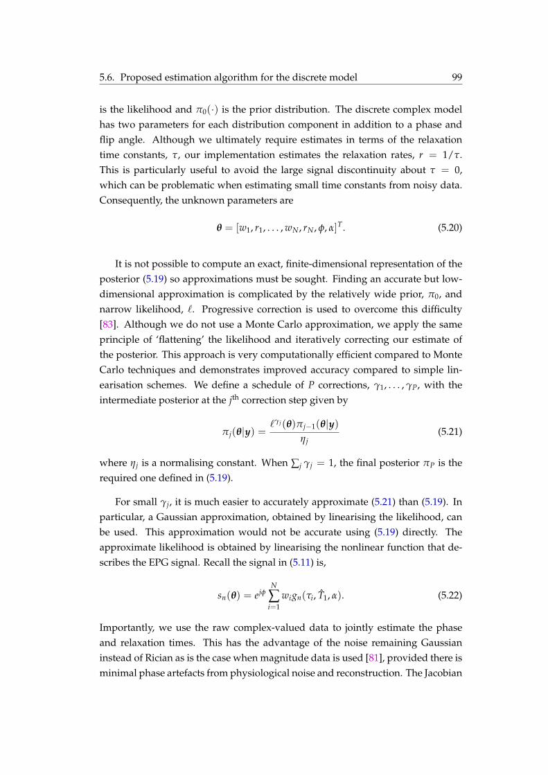
5.6. Proposed estimation algorithm for the discrete model 99
is the likelihood and π0(·) is the prior distribution. The discrete complex modelhas two parameters for each distribution component in addition to a phase andflip angle. Although we ultimately require estimates in terms of the relaxationtime constants, τ, our implementation estimates the relaxation rates, r = 1/τ.This is particularly useful to avoid the large signal discontinuity about τ = 0,which can be problematic when estimating small time constants from noisy data.Consequently, the unknown parameters are
θ = [w1, r1, . . . , wN , rN , φ, α]T. (5.20)
It is not possible to compute an exact, finite-dimensional representation of theposterior (5.195.19) so approximations must be sought. Finding an accurate but low-dimensional approximation is complicated by the relatively wide prior, π0, andnarrow likelihood, `. Progressive correction is used to overcome this difficulty[8383]. Although we do not use a Monte Carlo approximation, we apply the sameprinciple of ‘flattening’ the likelihood and iteratively correcting our estimate ofthe posterior. This approach is very computationally efficient compared to MonteCarlo techniques and demonstrates improved accuracy compared to simple lin-earisation schemes. We define a schedule of P corrections, γ1, . . . , γP, with theintermediate posterior at the jth correction step given by
πj(θ|y) =`γj(θ)πj−1(θ|y)
ηj(5.21)
where ηj is a normalising constant. When ∑j γj = 1, the final posterior πP is therequired one defined in (5.195.19).
For small γj, it is much easier to accurately approximate (5.215.21) than (5.195.19). Inparticular, a Gaussian approximation, obtained by linearising the likelihood, canbe used. This approximation would not be accurate using (5.195.19) directly. Theapproximate likelihood is obtained by linearising the nonlinear function that de-scribes the EPG signal. Recall the signal in (5.115.11) is,
sn(θ) = ejφN
∑i=1
wign(τi, T1, α). (5.22)
Importantly, we use the raw complex-valued data to jointly estimate the phaseand relaxation times. This has the advantage of the noise remaining Gaussianinstead of Rician as is the case when magnitude data is used [8181], provided there isminimal phase artefacts from physiological noise and reconstruction. The Jacobian

100 Chapter 5. Estimation of multi-component relaxation rate distributions
for the signal in (5.225.22) is
J(θ) =
∂s1∂w1
∂s1∂r1
· · · ∂s1∂wN
∂s1∂rN
∂s1∂φ
∂s1∂α
......
. . ....
......
...∂sM∂w1
∂sM∂r1
· · · ∂sM∂wN
∂sM∂rN
∂sM∂φ
∂sM∂α
(5.23)
The partial derivatives can be calculated efficiently using a set of recursive rela-tionships set out in Appendix 5.C5.C.
We adopt a Gaussian prior with mean, µ0, and covariance Ψ0. Further, πj−1 isassumed to be Gaussian with mean µj−1 and covariance matrix Ψj−1. The approx-imate likelihood is
ˆγj(θ) = N(
y; s(µj−1) + J(µj−1)(θ− µj−1), Σ/γj
)(5.24)
where J is the Jacobian in (5.235.23) andN (µ, Σ) denotes a multivariate Gaussian PDFwith mean µ and covariance Σ. In this case, the prior and likelihood are linearand Gaussian at each step. This is the same situation as a Kalman filter and thusthe posterior approximation is a Gaussian with mean and variance given by theKalman filter update equations,
µj = µj−1 + K j(y− s(µj−1)), (5.25a)
Ψj = (I − K j J)Ψj−1 (5.25b)
where I is the identity matrix and K j is the gain at the jth iteration defined as
K j = Ψj−1 J′(JΨj−1 J′ + Σ/γj)−1. (5.26)
Initially, the linearisation will be inaccurate but the likelihood will be wide duedo severe flattening, so the approximation of πj remains accurate. As the algo-rithm progresses, the approximate posterior approaches the true posterior and thelinearisation becomes more accurate. This process is very similar to simulatedannealing [8484] and we will see that the resulting algorithm is very robust to localminima, particularly at low SNR. The final algorithm is described in Algorithm 5.15.1.The algorithm is computationally efficient as matrix inversions can exploit the di-agonal nature of the measurement covariance.

5.6. Proposed estimation algorithm for the discrete model 101
Algorithm 5.1: Estimation Algorithm
Input: Data, y; Covariance, Σ = σ2 I; Prior, µ0, Ψ0; Correction schedule,γ1, . . . , γP
Output: Estimate, µP
1 for j← 1 . . . P do2 Calculate Jacobian, J ← J(µj−1)
3 Calculate gain, K j ← Ψj−1 J′(JΨj−1 J′ + Σ/γj)−1
4 Update mean, µj ← µj−1 + K j(y− s(µj−1))
5 Update covariance, Ψj ← (I − K j J)Ψj−1
5.6.1 Demonstration of algorithm
The operation of this algorithm is demonstrated with an example consisting a sin-gle discrete component with weight, w = 0.7, and relaxation time, τ = 100 ms. Theaim is to estimate these two values from 32 echo measurements spaced 12 ms apart.The prior distribution is relatively wide reflecting minimal knowledge about thetrue parameter values. We test two correction schedules: firstly we perform a sin-gle correction (γ1 = 1, P = 1) equivalent to Bayesian estimation using the standardExtended Kalman Filter equations. The second schedule consists of P = 30 correc-tions, logarithmically spaced between 10−6 and 1, i.e., γi = 106i/29−6, i = 0, . . . , 29and normalised such that ∑j γj = 1. The logarithmic spacing ensures that smallcorrections are made initially, when the linearised approximation can be poor, andprogressively larger corrections are performed as the estimates becomes more ac-curate.
Figure 5.5a5.5a displays error ellipses for the prior and the approximate posteriorderived using the linearised likelihood and a single correction step. The linearisa-tion occurs about the prior mean, which, in this case, is too far from the true pa-rameters to provide an accurate likelihood approximation. The resulting posteriorapproximation is poor and not representative of the true parameters. Figure 5.5b5.5billustrates the progressive corrections from the prior (at 0%) to the posterior (at100%). In this case, the flattening of the likelihood results in small updates to theposterior approximation indicated by the evolution of the error ellipse. The al-gorithm mitigates the difficulties of using a wide prior with a narrow likelihoodfunction and the final posterior approximation is very close to the true parameters.

102 Chapter 5. Estimation of multi-component relaxation rate distributions
0.1 0.2 0.3 0.4 0.5 0.6 0.7 0.8 0.9
0
5
10
15
20
25
30
weight, w
R2
(s−1 )
Prior
Prior mean
Approx posterior
Approx posterior mean
True params
(a)
0.1 0.2 0.3 0.4 0.5 0.6 0.7 0.8 0.9
0
5
10
15
20
25
30
weight, wR
2(s
−1 )
10%
20%
30%
40%
50%
60%
70%
80%
90%
100%
Numberofcorrectionscompleted
(b)
Figure 5.5: Error ellipses for the prior and posterior distributions demonstratingthe proposed algorithm using (a)(a) a single correction and (b)(b) a schedule of 30 cor-rections. The true parameters are marked with a × and the distribution mean isindicated by a •. The colours reflects the number of corrections performed where0% gives the prior and 100% gives the posterior approximation.
5.6.2 Simulations
In this work we define a Gaussian prior for two components with mean
µ0 = [0.7 0.1−1 0.3 0.02−1 0 2π/3]T, (5.27)
and covariance
Ψ0 =
12
1002
0.22
1002
352
352
. (5.28)
Recall the parameter vector in (5.205.20) is composed of weights, relaxation rates, aphase angle and a flip angle. The prior is relatively wide such that the estimationbias is negligible. A similar prior can be created for three or more components.The correction schedule is the same as above and consists of 30 corrections, loga-rithmically spaced between 10−6 and 1 and normalised such that ∑j γj = 1.
To examine the accuracy of different estimation algorithms for varying levelsof SNR, a decay curve was generated from a multicomponent distribution consist-

5.6. Proposed estimation algorithm for the discrete model 103
ing of two discrete modes: a slow component with weight 0.7 and T2 of 100 ms,and a fast component with weight 0.3 and T2 of 20 ms. These general features aretypical of white matter tissue in the cortex. A flip angle of 160 was simulated torepresent a non-ideal B1 field. The signal was calculated from the extended phasegraph (EPG) algorithm to model secondary and stimulated echoes as describedby (5.115.11) and (5.45.4). Simulations consisted of 2000 independent trials where i.i.d.complex noise was added. The phase angle in (5.115.11) was randomly selected eachtrial from a uniform distribution between −π and π to demonstrate that the al-gorithm is insensitive to phase. The relaxation modes were estimated using threeapproaches: a discrete grid model with NNLS including stimulated echo com-pensation, as in [7777]; a discrete model with a gradient based MLE optimisationsimilar to [7979] extended to multiple components; and the discrete model using theproposed Bayesian algorithm. The iterative MLE algorithm was initialised at theprior mean in (5.275.27). To compare the continuous NNLS distributions, componentlocations were extracted using the geometric mean between 0 ms and 40 ms for thefast component and 40 ms and 200 ms for the slow component [7575]. The MSE wascalculated and the process was repeated for 30 SNR values logarithmically spacedbetween 10 and 1000. Average execution times for the three algorithms were cal-culated from all trials.
The ability to estimate a wide range of flip angles was examined by anothersimulation of 2000 trials with an SNR of 300 (as in [7777]) for 30 flip angles evenlyspaced between 60 and 180. The MSE was calculated at each flip angle forthe three algorithms. Fig. 5.65.6 displays the performance of the NNLS algorithm,a gradient based MLE algorithm and the proposed Bayesian algorithm. This plotdemonstrates that the MLE optimisation algorithm achieves the same performanceas the Bayesian algorithm for sufficiently high SNR. This is expected for a suffi-ciently wide prior, when the MLE and MAP estimates converge. However, theMLE algorithm fails to produce reliable estimates at low SNR values, due to anoptimisation cost function that is poorly behaved (it is relatively flat with localminima). NNLS exhibits suboptimal performance, although it achieves reasonableresults across a range of SNR values.
Both the proposed algorithm and NNLS are reasonably robust to flip anglevariations. Fig. 5.75.7 illustrates that the error in the estimated flip angle increaseswith the true flip angle. This can be understood by noting that the derivative of thesignal tends to zero as the flip angle approaches 180. The 8-point NNLS algorithmas implemented in [7777] exhibits elevated error around 80 and 160. This is due tothe algorithm testing only 8 flip angles and using spline interpolation to extractthe minimum sum of squares error. A smooth curve using 64 test angles displays

104 Chapter 5. Estimation of multi-component relaxation rate distributions
101
102
103
10−4
10−3
10−2
10−1
100
SNR (1/σ)
RMSE
(ms)
BayesianMLENNLS
Figure 5.6: The root mean squared error (RMSE) of the estimated T2 componentscalculated at different SNR values for the Bayesian algorithm (solid line), the gra-dient based MLE (dotted line) and NNLS (dashed line).
60 80 100 120 140 160 180
1
2
3
4
5
6
Flip angle (degrees)
RMSE
(×10
−2degrees)
BayesianNNLS 8 pointsNNLS 64 points
Figure 5.7: The RMSE of flip angles estimated from multiecho data with an SNRof 300. The error is plotted against different values of the true flip angle for theBayesian algorithm (solid line) and the NNLS algorithm with 8 (dotted line) and64 (dashed line) interpolation points.

5.6. Proposed estimation algorithm for the discrete model 105
only slightly degraded performance compared to the proposed algorithm. Thismodest gain in performance, however, increases the computation time of NNLSby an order of magnitude.
The Bayesian algorithm proposed above had an average execution time of0.022 s per voxel compared to NNLS with 8-point stimulated echo correction, whichaveraged 0.17 s per voxel. This represents an almost eight-fold improvement.
5.6.3 Optic nerve experiments
All experiments were performed on a 4.7 T Bruker BioSpec small bore MRI scannerfitted with a high performance gradient set. A cryogenically cooled surface coilwas used to improve SNR. A multi-echo CPMG sequence with 24 echoes was runwith a first echo time of 12 ms and an echo spacing of 12 ms. The slice thicknesswas 1 mm for all experiments.
A sample was constructed consisting of agar gel with a sheep optic nerve fixedparallel to the transverse plane. The TR = 2500 ms, FOV = 6.4 mm × 12.8 mmwith a matrix size of 64× 128. B1 field mapping was performed by processing twospin echo images acquired with different excitation flip angles as in [8585]. Data wasprocessed with the proposed algorithm using both the exponential model, whichassumes ideal 180 flip angles; and the EPG model, which jointly estimates theT2 components, weights and B1 map. The algorithms were run for both a singlecomponent distribution and a two component distribution.
The B1 maps for the optic nerve sample are displayed in Fig. 5.85.8. The B1 mapgenerated from the proposed estimation algorithm is consistent with that gener-ated from a low resolution B1 field mapping protocol. The estimated maps are verysimilar for a single component distribution and a two component distribution. Thenature of the surface coil creates a dramatic flip angle inhomogeneity throughoutthe sample, with only a small region exhibiting a flip angle close to the prescribed180. Note that regions above the 180 arc experience a flip angle greater than 180
but are reflected about 180 as this is equivalent in the signal model.
Fig. 5.95.9 presents the single component T2 maps generated with different sig-nal models. Fig. 5.9a5.9a displays the single T2 value estimated using the EPG algo-rithm, which models stimulated echoes resulting from nonideal flip angles. Theestimated T2 value is similar along the length of the optic nerve, despite the largeflip angle variation demonstrated in Fig. 5.85.8. Conversely, Fig. 5.9b5.9b shows the re-sults of an exponential decay model that neglects flip angle inhomogeneity. The T2
maps in this case are overestimated by an increasing amount as the flip angle de-viates from the ideal 180. Figure 5.9c5.9c displays the T2 profiles along a line through

106 Chapter 5. Estimation of multi-component relaxation rate distributions
B1 map (degrees)
30 60 90 120 150 180
(a)
Figure 5.8: The B1 map (left) estimated using a single component model, (middle)estimated using a multi-component model and (right) measured from separatespin echo images.
0
10
20
30
40
50
60
70
80
90
(a)
0
10
20
30
40
50
60
70
80
90
(b)
0 20 40 60 80 100 120 140
0
10
20
30
40
50
60
70
80
90
Sl ice posi tion
T2
T2 EPGT2 EXP
(c)
Figure 5.9: The single component T2 maps (ms) of an optic nerve sample estimatedfrom (a)(a) the extended phase graph (EPG) model and (b)(b) the exponential decaymodel (EXP). Profiles along the dashed lines of the T2 estimates are shown in (c)(c).

5.6. Proposed estimation algorithm for the discrete model 107
the optic nerve. This demonstrates the close match between estimates when theflip angle is close to 180 and the overestimation as the flip angle decreases. Thisresult is consistent with those previously reported in [7777, 7979].
Fig. 5.105.10 presents the multicomponent T2 maps generated with different signalmodels. Fig. 5.10a5.10a displays the two components estimated using the EPG algo-rithm. The estimated T2 values are similar along the length of the optic nerve,despite the large flip angle variation. Conversely, Fig. 5.10b5.10b displays the T2 com-ponents from an exponential decay model that neglects flip angle inhomogeneity.The T2 maps in this case exhibit a large variation along the nerve, with the fastcomponent fitted in an attempt fix the disparity of the first few echo amplitudesresulting from stimulated echoes. T2 profiles along the nerve from both algorithmsis displayed in Figure 5.10c5.10c. As expected the estimates are similar in regions cor-responding to flip angles close to 180. In other regions, however, the model mis-match causes large variation dependent more on the flip angle than the underlyingstructure.
5.6.4 Mouse brain experiments
An ex-vivo mouse brain was scanned with the same 24 echo sequence with TR =
2500 ms, FOV = 15 mm× 15 mm and a matrix size of 192× 192 for an in-planeresolution of 78.1 µm. A single mid-axial slice of 1 mm was acquired. This datawas processed with the proposed algorithm using the EPG model and the NNLSmodification in [7777]. Both algorithms attempt to estimate multicomponent distri-butions and account for stimulated echoes by estimating both the T2 distributionand the B1 map. As described above, T2 values were extracted from the NNLSdistribution using the geometric mean to obtain location estimates of the fast andslow components as in [7575].
To further investigate the reliability of the gradient based MLE algorithm, com-plex noise was added to the mouse data to yield an SNR of 200. This data wasthen processed with the proposed algorithm and a gradient based MLE algorithm.Fig. 5.11a5.11a displays boxplots of the T2 value of the first component for the two al-gorithms. The plots depict the median, first and third quartiles, and values con-sidered outliers. The estimates from the MLE optimisation and the Bayesian algo-rithm are similar, as shown by similar medians and first and third quartiles. How-ever, approximately 6% of the MLE estimates can be considered outliers, manyof which are far away from the true value. These outliers manifest as erroneousspeckled values in the T2 map, as illustrated in Fig. 5.11b5.11b.
Estimation results from the mouse brain data are displayed in Fig. 5.125.12. Estimated

108 Chapter 5. Estimation of multi-component relaxation rate distributions
0
10
20
30
40
50
60
(a)
0
10
20
30
40
50
60
(b)
0 20 40 60 80 100 120 140
0
10
20
30
40
50
60
Slice position
T2
Ts2 EPG
Ts2 EXP
Tf2 EPG
Tf2 EXP
(c)
Figure 5.10: The multicomponent T2 maps (ms) of an optic nerve sample esti-mated from (a)(a) the extended phase graph (EPG) model and (b)(b) the exponentialdecay model (EXP). The left and right sides display the slow and fast components,respectively. Profiles along the dashed lines of the T2 estimates for the differentcomponents are shown in (c)(c).

5.6. Proposed estimation algorithm for the discrete model 109
40
60
80
100
120
140
160
Bayesian MLE
T2estimate
(ms)
(a)
0
10
20
30
40
50
60
70
T2(m
s)
(b)
Figure 5.11: Analysis of outliers from a gradient based optimisation algorithm.(a)(a) displays a summary of the different estimates in the region of interest for theBayesian algorithm and the gradient based MLE algorithm. (b)(b) displays the regionof interest of the mouse brain estimates for the (top) Bayesian and (bottom) MLEalgorithms.
values from the proposed algorithm are shown in the top image of each figure part,while the bottom image displays values extracted from the NNLS distribution. Theweights and times of the slow component (calculated using the geometric meanbetween 40 ms and 200 ms) are displayed in Figs. 5.12a5.12a and 5.12b5.12b, respectively.The Bayesian and NNLS algorithms produce similar T2 maps for this component.Figs. 5.12c5.12c and 5.12d5.12d display the fast component and demonstrate an essentialdifference between the two algorithms. The maps produced by the proposed al-gorithm contain anatomical features such as a decreased T2 below the ventricles,consistent with the presence of white matter. Fast components above 40 ms arenot displayed. NNLS fast T2 maps were calculated between 0 ms and 40 ms andexhibit a relatively constant T2 value. NNLS appears to represent the white matterby increasing the weighting of the relatively constant T2. This is due to the regu-larisation of the NNLS algorithm which decreases the estimation variance at theexpense of increased bias. On the other hand, the proposed algorithm producesa fast component with both an increased weight and a decreased time constant inthe white matter region. It is worthwhile to mention that both algorithms oftenproduce fast component weights close to zero as shown in Fig. 5.12c5.12c. In this case,the T2 estimates of the corresponding voxels are unlikely to be reliable since theyhave minimal contribution to the fitted signal.
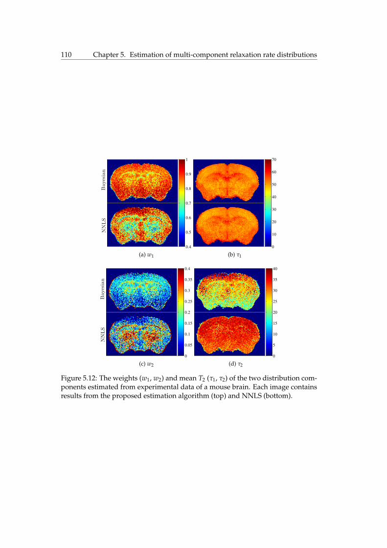
110 Chapter 5. Estimation of multi-component relaxation rate distributions
0.4
0.5
0.6
0.7
0.8
0.9
1
NNLS
Bayesian
(a) w1
0
10
20
30
40
50
60
70
(b) τ1
0
0.05
0.1
0.15
0.2
0.25
0.3
0.35
0.4
NNLS
Bayesian
(c) w2
0
5
10
15
20
25
30
35
40
(d) τ2
Figure 5.12: The weights (w1, w2) and mean T2 (τ1, τ2) of the two distribution com-ponents estimated from experimental data of a mouse brain. Each image containsresults from the proposed estimation algorithm (top) and NNLS (bottom).

5.6. Proposed estimation algorithm for the discrete model 111
5.6.5 Model selection
The algorithm proposed above assumes the number of distribution components isknown. Fitting too few or too many components will result in degraded perfor-mance and this could be considered the main disadvantage of the discrete distri-bution model. For example, the weights of the fast T2 component were estimatedclose to zero in the agar gel region of the optic nerve sample. This is due to thefact that the relaxation curve of the gel is described accurately by a single decayingcomponent. It would be preferable to only fit a single component in this case, asthe second component is simply fit to the noise and has minimal contribution tothe signal. There are many model selection techniques that choose the appropriatemodel order automatically based on a statistical metric, see e.g. [8686, 8787]. A simplemeasure known as the Bayesian Information Criteria (BIC) [8888] is defined as
BIC(M) = −2 ln(`M) + kM ln(M) (5.29)
where `M is maximum value of the likelihood function for model M, kM is thenumber of parameters to fit and M is the number of measurements.
Although this criteria is based on the maximum likelihood estimate (MLE) ofeach candidate model, we use the proposed Bayesian algorithm. Under certainnon-restrictive conditions, the Bayesian estimate asymptotically converges to theMLE [8989]. This justifies the use of the Bayesian estimate in place of the MLE, andthe reliability it provides. We evaluate the BIC at each pixel in the optic nerve datafor two models: a single component model and a two-component model, bothwith stimulated echo correction using the EPG algorithm. In general, the modelwith smallest BIC is preferred as it provides a good tradeoff between model com-plexity and model fit. The BIC difference between the models gives a quantitativemeasure of support for the two models.
Figure 5.135.13 displays the BIC difference between the one and two componentmodels. In the agar gel region of the sample, there is minimal difference betweenthe models suggesting that the data is accurately represented by a single compo-nent. Conversely, the optic nerve displays a large negative difference between theone component and two component model. This provides strong support for a twocomponent model. As the signal strength decreases further away from the surfacecoil, the strength of support for a two component model decreases as the criteriacannot discern between the model and noise. Nonetheless, these results suggestthat automatic model selection techniques such as the BIC may prove useful forthe estimation of multi-component T2 distributions.

112 Chapter 5. Estimation of multi-component relaxation rate distributions
Figure 5.13: (left) Magnitude image of the optic nerve sample acquired with a sur-face coil and (right) the difference between Bayesian Information Criteria metricsbetween the two component model and the one component model. Large negativevalues indicate strong evidence for the two component model.
5.7 Optimal experiment design
This section addresses an often overlooked question: how to optimise the acqui-sition sequence for T2 estimation. Previous work in [9090] considered the joint esti-mation of T1, T2 and M0 and optimised sequence parameters to give the minimumestimation variance. The study was limited to a single component per pixel. Inthis work, we consider sequence optimisation in the context of multicomponentT2 distribution estimation using a CPMG sequence.
The CPMG sequence parameters we can control are the first echo time, t1, echospacing, ∆t, and number of echoes, M. Unfortunately, the optimal selection ofthese parameters depends on the unknown T2 components we wish to estimate.The Cramér-Rao lower bound (CRLB) was calculated in Section 5.5.15.5.1 to analysethe estimation variance for multicomponent T2 distributions. In this section, weemploy the CRLB to select the sequence parameters that give the lowest possiblevariance.
The CRLB is defined by the inverse of the Fisher information matrix (FIM). Ingeneral, the inverse FIM can be written as a function of the unknown T2 compo-nents, θ, and the experimental design parameters, ϑ, denoted F−1(θ; ϑ). Variousoptimisation problems can be defined to find the optimal sequence parameters, ϑ.For example, we may wish to minimise the worst case sum of variances over arange of T2 components. That is,
ϑ = arg minϑ
(maxθ∈Θ
Tr
F−1(θ; ϑ))
(5.30)

5.7. Optimal experiment design 113
10 20 30 40 50 60
0
5
10
15
20
25
30
35
40
45
50
Number of echoes
CRLB
(ms)
T2 = 50 msT2 = 100 msT2 = 200 msT2 = 500 msT2 = 1000 ms
(a)
10 20 30 40 50 60
0
0.005
0.01
0.015
0.02
0.025
0.03
0.035
0.04
0.045
0.05
Number of echoes
Cost
T2 = 50 ms
T2 = 100 ms
T2 = 200 ms
T2 = 500 ms
T2 = 1000 ms
(b)
Figure 5.14: (a)(a) The CRLB displaying a monotonic performance improvement forincreasing number of echoes and (b)(b) a cost function consisting of CRLB and a linearpenalty term for number of echoes. The coloured curves represent different T2values.
where Θ is the set of T2 components that we expect to encounter and Tr denotes thematrix trace (equivalent to the sum of variances). For the present study, we con-sider a simpler problem and aim to determine the optimal sequence for a givenT2 distribution. This problem is equivalent to (5.305.30) when Θ contains a single ele-ment.
The first question we consider is how many echoes to acquire. For this prob-lem we fix the first echo time and inter-echo spacing at 10 ms and optimise overthe number of echoes. We consider a single component distribution with data ac-quired with an SNR of 100. Figure 5.14a5.14a displays the CRLB as a function of thenumber of echoes. The notion that acquiring echoes in the “noise floor” can de-grade T2 estimation is only applicable when magnitude data is used. The perfor-mance of the full model using complex measurements is monotonic in the num-ber of echoes. Although the estimation performance never degrades with extraechoes, the increase in performance tends to zero as the signal becomes noise. Fig-ure 5.14b5.14b illustrates a cost function consisting of the CRLB and a linear penaltyterm for the number of echoes. This penalty term could model practical factorssuch as an increase in the RF power deposition for additional echoes. In this case,the optimal number of echoes is finite and increases as the T2 value increases. Forexample, with our chosen penalty, 10 echoes is optimal to estimate a single compo-nent with T2 = 200 ms while 22 echoes may be preferred to estimate a componentwith T2 = 500 ms. Results will vary strongly depending on the choice of penaltyso care must be taken in selecting an appropriate penalty for a given application.
The second sequence parameter we optimise is the echo spacing. We assume

114 Chapter 5. Estimation of multi-component relaxation rate distributions
0 5 10 15 20 25 30
0
2
4
6
8
10
12
14
16
18
20
Echo spacing (ms)
CRLB
(ms)
(a) (b)
Figure 5.15: (a)(a) The CRLB for different echo spacings for a two component distri-bution with τ1 = 20 ms and τ2 = 100 ms. The optimal spacing is marked with acircle. (b)(b) displays the optimal echo spacing as a function of the two components.A linear fit to this function is displayed as a grid overlay.
the number of echoes is fixed at 32, and we aim to determine the optimal echospacing for different T2 distributions. In this case, we adopt a brute force approachand calculate the optimal spacing for all pairs of T2 components. Figure 5.15a5.15aillustrates this optimisation for a single pair representing a two component distri-bution with τ1 = 20 ms and τ2 = 100 ms. The optimal echo spacing in this casemust trade the estimation accuracy between fast and slow components. The min-imum estimation variance is obtained when the echo spacing is ∼8 ms. We therepeat this optimisation for all practical values of the fast and slow componentsof a multi-component distribution. Figure 5.15b5.15b depicts the optimal echo spacingas a function of the two distribution components. This function is reasonably wellapproximated by a plane shown as a grid overlay. The least squares fitting of thisplane to the optimal function gives the following approximate relationship,
(∆t)opt ≈ 0.1(τ1 + τ2) (5.31)
This relationship is useful to determine the optimal echo spacing (given a total of32 echoes) for accurate estimation of two given T2 components. A similar analysiscould be performed for non-uniform echo spacing although this increases size ofthe parameter space to optimise.
This section has explored two examples of optimal experiment design using theCramér-Rao lower bound as a cost function. This demonstrates that experimentdesign should be considered jointly with the problem of T2 distribution estimation.

5.8. Discussion and conclusion 115
5.8 Discussion and conclusion
The estimation of T2 distributions from CPMG data is a challenging problem. Inthis chapter, we have developed a parametric and continuous model for multi-component T2 distribution analysis and used it to show that it is infeasible to accu-rately estimate the width of a continuous distribution. Instead we have considereda discrete distribution together with the extended phase graph (EPG) algorithm toaccount for nonideal flip angles and the resulting stimulated echoes. We havedemonstrated that a simple gradient-based MLE algorithm is unsuitable in thiscase and developed a Bayesian alternative that exhibits near-optimal performanceeven at very low SNR. The proposed algorithm jointly estimates the weights andlocations of the T2 components as well as the signal phase and refocusing flip an-gle.
It is commonly thought that the regularisation in NNLS produces ‘more real-istic’ distributions, primarily due to the smooth and continuous nature of the re-sulting curves [7777]. In this work, however, we have shown that one cannot reliablyestimate the distribution width, thus a regularised distribution, although continu-ous, is not necessarily closer to the true distribution than a discrete counterpart.
The distributions resulting from the NNLS algorithm have been most useful todate by extracting summary statistics, such as the mean intra/extra-cellular peakand the myelin water fraction [7575]. These measures integrate the distribution andconsequently are only weakly dependent on the estimated width. Our analysisjustifies the use of these statistics, as these features can be reasonably well esti-mated, despite minimal knowledge of the distribution width. However, we haveshown that regularisation can bias the distribution shape of the fast components,leading to a lack of anatomical information in the T2 maps.
One drawback of the discrete multicomponent T2 model is the need to know apriori the number of components. For example, the weights of the fast T2 compo-nent were estimated close to zero in the agar gel region of the optic nerve sample(results not shown). This is due to the fact that the relaxation curve of the gel isdescribed accurately by a single decaying component. It would be preferable toonly fit a single component in this case, as the second component is simply fit tothe noise and has minimal contribution to the signal. Many model order selectiontechniques exist, such as the Akaike or Bayesian information criteria, that choosean appropriate model order based on a statistical metric, see e.g. [8787]. These crite-ria are applicable to MRI signal decay data although this is beyond the scope thisthesis.
In the presence of non-ideal flip angles, the estimated T2 components for a

116 Chapter 5. Estimation of multi-component relaxation rate distributions
discrete distribution with an exponential decay function exhibit more complicatedbehaviour than the single component counterpart. For a single component, theT2 value was increasingly overestimated as the flip angle deviated from 180 asreported in [7979]. In the case when a two component distribution was used, thesecond component is estimated to compensate for the stimulated echoes. Thisresults in a large variation of the second component and relatively small variationof the first component.
The advantage of the discrete distribution model is that the associated estima-tion problem is inherently better conditioned than the NNLS pseudo-continuousgrid model. This reduces the need for regularisation and potentially minimises theestimation bias. The minimal regularisation is apparent in our Bayesian approachsince the prior distribution for the unknown parameters is relatively wide. Addi-tionally, the proposed algorithm requires substantially less computation comparedto both gradient-based optimisation and the NNLS algorithm.
The EPG signal model together with the proposed estimation algorithm makesquantitative multicomponent T2 analysis viable in the presence of large B1 inho-mogeneity, such as those produced from a transceive surface coil.

5.A. Signal model for inverse-gamma mixture 117
Appendices
5.A Signal model for inverse-gamma mixture
The measured signal from a distribution consisting of an inverse-gamma mixtureis derived from the general measurement equation,
yn = ejφ∫ ∞
0f (τ)e−t/τdτ (5.32)
Substituting the inverse gamma mixture gives,
yn = ejφ∫ ∞
0
N
∑i=1
wiβαi
iΓ(αi)
τ−αi−1e−βi/τe−t/τdτ (5.33)
= ejφN
∑i=1
wiβαi
iΓ(αi)
∫ ∞
0τ−αi−1e−(t+βi)/τdτ (5.34)
Let u = (t + βi)/τ. Taking derivatives gives,
dτ = − (t + βi)
u2 du (5.35)
Changing the variable of integration, and noting the new limits of −∞ to 0, gives,
yn = ejφN
∑i=1
wiβαi
iΓ(αi)
∫ 0
−∞
(t + βi
u
)−αi−1
e−u−(t + βi)
u2 du (5.36)
= ejφN
∑i=1
wiβαi
iΓ(αi)
(t + βi)−αi−1(t + βi)
∫ ∞
0uαi−1e−udu (5.37)
= ejφN
∑i=1
wiβαi
i Γ(αi)
(t + βi)αi Γ(αi)(5.38)
= ejφN
∑i=1
wi
(βi
t + βi
)αi
(5.39)
5.B The extended phase graph algorithm
The extended phase graph algorithm is a recursive algorithm that tracks the evo-lution of the phase coherence pathways [7272]. It describes the spin system at agiven time by a distribution over different phase states. There are three types ofstates, F(n)
k (dephasing), F(n)−k (rephasing) and Z(n)
k (longitudinal) for each coher-ence level, k, and echo number, n. After the initial excitation pulse, all the mag-netisation is assumed to be coherent and on the transverse plane so F(0)
0 = 1 and
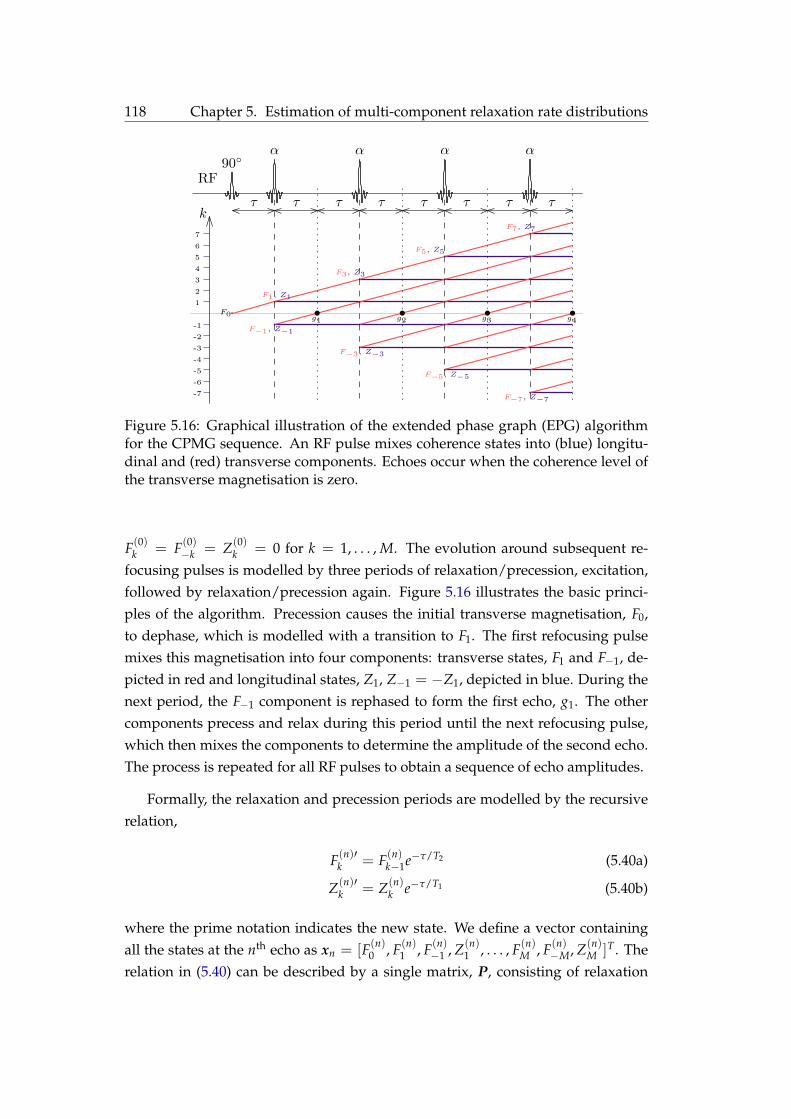
118 Chapter 5. Estimation of multi-component relaxation rate distributions
90
RF
α
τ τ
α
τ τ
α
τ τ
α
τ τk
F0
1
2
3
4
5
6
7
-7
-6
-5
-4
-3
-2
-1g1 g2 g3 g4
F3, Z3
F−3, Z−3
F−1, Z−1
F1, Z1
F5, Z5
F−5, Z−5
F7, Z7
F−7, Z−7
Figure 5.16: Graphical illustration of the extended phase graph (EPG) algorithmfor the CPMG sequence. An RF pulse mixes coherence states into (blue) longitu-dinal and (red) transverse components. Echoes occur when the coherence level ofthe transverse magnetisation is zero.
F(0)k = F(0)
−k = Z(0)k = 0 for k = 1, . . . , M. The evolution around subsequent re-
focusing pulses is modelled by three periods of relaxation/precession, excitation,followed by relaxation/precession again. Figure 5.165.16 illustrates the basic princi-ples of the algorithm. Precession causes the initial transverse magnetisation, F0,to dephase, which is modelled with a transition to F1. The first refocusing pulsemixes this magnetisation into four components: transverse states, F1 and F−1, de-picted in red and longitudinal states, Z1, Z−1 = −Z1, depicted in blue. During thenext period, the F−1 component is rephased to form the first echo, g1. The othercomponents precess and relax during this period until the next refocusing pulse,which then mixes the components to determine the amplitude of the second echo.The process is repeated for all RF pulses to obtain a sequence of echo amplitudes.
Formally, the relaxation and precession periods are modelled by the recursiverelation,
F(n)′k = F(n)
k−1e−τ/T2 (5.40a)
Z(n)′k = Z(n)
k e−τ/T1 (5.40b)
where the prime notation indicates the new state. We define a vector containingall the states at the nth echo as xn = [F(n)
0 , F(n)1 , F(n)
−1 , Z(n)1 , . . . , F(n)
M , F(n)−M, Z(n)
M ]T. Therelation in (5.405.40) can be described by a single matrix, P, consisting of relaxation
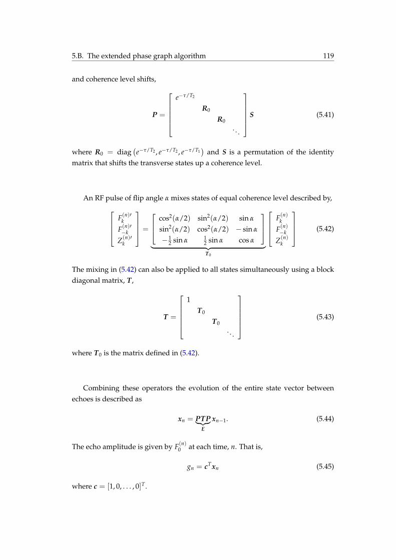
5.B. The extended phase graph algorithm 119
and coherence level shifts,
P =
e−τ/T2
R0
R0. . .
S (5.41)
where R0 = diag(e−τ/T2 , e−τ/T2 , e−τ/T1
)and S is a permutation of the identity
matrix that shifts the transverse states up a coherence level.
An RF pulse of flip angle α mixes states of equal coherence level described by,F(n)′
k
F(n)′−k
Z(n)′k
=
cos2(α/2) sin2(α/2) sin α
sin2(α/2) cos2(α/2) − sin α
− 12 sin α 1
2 sin α cos α
︸ ︷︷ ︸
T0
F(n)
k
F(n)−k
Z(n)k
(5.42)
The mixing in (5.425.42) can also be applied to all states simultaneously using a blockdiagonal matrix, T ,
T =
1
T0
T0. . .
(5.43)
where T0 is the matrix defined in (5.425.42).
Combining these operators the evolution of the entire state vector betweenechoes is described as
xn = PTP︸︷︷︸E
xn−1. (5.44)
The echo amplitude is given by F(n)0 at each time, n. That is,
gn = cTxn (5.45)
where c = [1, 0, . . . , 0]T.

120 Chapter 5. Estimation of multi-component relaxation rate distributions
5.C Partial derivatives
The derivative of the echo amplitude with respect to the unknown parametersis useful for a number of applications including CRLB analysis, gradient descentoptimisation and approximations of the likelihood. As such, an efficient means tocompute the partial derivatives is included here.
The recursion in (5.445.44) is linear in the state vector thus the partial derivativescan also be calculated in a recursive manner. First notice that both xn and E dependon the parameter of interest, θ, so the product rule must be applied,
∂xn
∂θ=
∂E∂θ
xn−1 + E∂xn−1
∂θ. (5.46)
Next we use the decomposition P = P(r1, r2) and T = T(α). The partial derivativeof the matrix elements in E = PTP are
∂E∂α
= P∂T∂α
P, (5.47)
∂E∂r2
=∂P∂r2
TP + PT∂P∂r2
. (5.48)
For convenience we define additional intermediate states x(r)n , x(α)n , z(r)i and z(α)i
to calculate the different terms in (5.465.46)–(5.485.48). We also let P′ = ∂P∂r2
and T ′ = ∂T∂α .
The recursive algorithm is shown in Algorithm 5.25.2. Note that the operators P, P′,T and T ′ can be executed very efficiently using the inherent structure described in(5.405.40) and (5.425.42). The derivatives of the EPG signal are simply the first element ofthe derivatives of the state vector, ∂xn/∂r2 and ∂xn/∂α.

5.C. Partial derivatives 121
Algorithm 5.2: Recursive algorithm for EPG derivativesInput: Relaxation parameters, r1 = 1/T1, r2 = 1/T2; Flip angle, αOutput: Partial derivatives, ∂xn
∂r2and ∂xn
∂α for n = 1, . . . , M1 Calculate matrices, P and T using (5.415.41) and (5.435.43)2 Calculate derivatives, P′ = ∂P
∂r2and T ′ = ∂T
∂α
3 for n← 1 . . . M do// Calculate first term of product rule
4 z(r)n ← PTP′xn−1
5 z(α)n ← PT ′Pxn−1// Calculate second term of product rule
6 x(r)n ← PTP ∂xn−1∂r2
7 x(α)n ← PTP ∂xn−1∂α
// Combine terms for the derivatives
8 ∂xn∂r2← 2z(r)n + x(r)n
9 ∂xn∂α ← z(α)n + x(α)n// Calculate state evolution
10 xn ← PTPxn−1


Part III
Nonlinear Spatial Encoding
123


CHAPTER 6
Region-specific trajectory designusing nonlinear encoding fields
Contents6.1 Introduction . . . . . . . . . . . . . . . . . . . . . . . . . . . . . . . . . 125125
6.1.1 Notation . . . . . . . . . . . . . . . . . . . . . . . . . . . . . . . 127127
6.2 Theory . . . . . . . . . . . . . . . . . . . . . . . . . . . . . . . . . . . . 1271276.2.1 Local k-space . . . . . . . . . . . . . . . . . . . . . . . . . . . . 129129
6.3 Existing nonlinear encoding techniques . . . . . . . . . . . . . . . . 1301306.3.1 Cartesian PatLoc . . . . . . . . . . . . . . . . . . . . . . . . . . 131131
6.3.2 O-Space . . . . . . . . . . . . . . . . . . . . . . . . . . . . . . . 133133
6.3.3 4D-RIO . . . . . . . . . . . . . . . . . . . . . . . . . . . . . . . . 134134
6.4 Region specific trajectory design . . . . . . . . . . . . . . . . . . . . . 1341346.4.1 Trajectory optimisation . . . . . . . . . . . . . . . . . . . . . . 135135
6.4.2 Encoding fields and target regions . . . . . . . . . . . . . . . . 139139
6.4.3 Simulations . . . . . . . . . . . . . . . . . . . . . . . . . . . . . 142142
6.4.4 Experiments . . . . . . . . . . . . . . . . . . . . . . . . . . . . . 143143
6.4.5 Calibration . . . . . . . . . . . . . . . . . . . . . . . . . . . . . . 144144
6.4.6 Safety considerations . . . . . . . . . . . . . . . . . . . . . . . . 146146
6.5 Results . . . . . . . . . . . . . . . . . . . . . . . . . . . . . . . . . . . . 1461466.5.1 Trajectory optimisation and simulations . . . . . . . . . . . . . 146146
6.5.2 Experiments . . . . . . . . . . . . . . . . . . . . . . . . . . . . . 150150
6.6 Discussion . . . . . . . . . . . . . . . . . . . . . . . . . . . . . . . . . . 1521526.7 Conclusion . . . . . . . . . . . . . . . . . . . . . . . . . . . . . . . . . 156156
6.1 Introduction
SPATIAL encoding in MRI is traditionally achieved using magnetic fields withlinear gradients, applied to each of the three spatial dimensions. The linear
gradient fields in these schemes are typically setup to acquire samples of the object
125

126 Chapter 6. Region-specific trajectory design using nonlinear encoding fields
in the Fourier domain, or k-space, as described in Chapter 33. Image reconstruc-tion for this approach is straightforward and based on the inverse discrete Fouriertransform (DFT). This supports one’s intuition regarding the relationship betweensampling parameters and image properties such as SNR and resolution. Impor-tantly, the trade-off between SNR and resolution can be characterised precisely.
Recently, magnetic fields that vary nonlinearly across the field-of-view havebeen proposed to improve on the linear gradient approaches. The concept ofPatLoc (Parallel Imaging Technique using Localized Gradients) uses higher ordernon-bijective encoding fields with the potential to overcome safety limits associ-ated with peripheral nerve stimulation [99]. Similar to conventional SENSE imag-ing, the encoding inherent in the receiver coils is crucial to resolving the ambigu-ity associated with non-bijectivity. For a Cartesian PatLoc acquisition, the use ofambiguous encoding fields together with multiple RF coils provides an attractivealternative for acquisition acceleration compared to traditional undersampling inparallel imaging [1010]. In both cases reduced imaging time is achieved since thenon-bijective encoding leads to a reduced field-of-view, which requires fewer sam-ples for the same resolution. An important feature of a Cartesian PatLoc trajectoryis the spatially varying resolution. Since the quadrupolar fields have a large gra-dient at the periphery of the field-of-view, this region has improved resolution.Conversely, the quadrupolar fields provide no spatial encoding at the centre of thefield-of-view (where the gradient is zero) and the resolution is severely degraded,resulting in pronounced blurring.
O-Space imaging [1111] and Null Space Imaging [9191] use nonlinear fields withthe aim to provide spatial encoding that complements the spatial encoding pro-vided by multiple RF coil sensitivities. O-Space imaging uses a quadratic encod-ing field in conjunction with traditional linear fields. The linear fields translate thequadratic encoding function after each excitation. Consequently, projections areacquired along rings evolving outward from each centre point [1111]. It is purportedthat the improved encoding along the radial direction complements the inherentencoding provided by the receive coils along the azimuthal direction, allowing formuch faster imaging times. Null Space Imaging searches for the optimal encod-ing shapes using a singular value decomposition of the coil sensitivity matrix. Ingeneral the optimal encoding shapes cannot be realised with the available hard-ware, so a least square fit is performed to determine the closest achievable encod-ing shapes to use for projection imaging [9191]. This scheme promises to accelerateimage acquisition even further.
4D-RIO is a new PatLoc encoding strategy that uses linear and nonlinear fieldssimultaneously [1212]. Two out-of-phase radial trajectories are implemented on the

6.2. Theory 127
linear and quadrupolar pairs such that the linear gradient is maximum when thenonlinear gradient is minimum and vise versa. The reconstructed images exhibitrelatively uniform resolution compared to a Cartesian PatLoc trajectory withoutlinear fields.
This chapter develops a novel acquisition strategy that improves the resolutionin a region of interest. The technique uses nonlinear encoding fields; however,in contrast to existing techniques, this is the first method to design the acquisi-tion around the desired resolution. The trajectory design is posed as an optimisa-tion problem, which can be solved numerically, to produce a customised trajectorybased on the specified region of interest.
The chapter is organised as follows. Section 6.26.2 presents the theory of spatialencoding using multiple encoding fields with arbitrary shapes. The theory canbe considered a generalisation of that presented in Section 3.43.4. Section 6.36.3 exam-ines the existing nonlinear encoding strategies of Cartesian PatLoc, O-Space, and4D-RIO. This serves to highlight some basic properties of nonlinear spatial encod-ing. Section 6.46.4 develops a novel acquisition strategy that uses nonlinear encodingfields to enhance the resolution in a user-specified region and Section 6.56.5 verifiesthe technique through simulation and experiments.
6.1.1 Notation
Table 6.16.1 lists the important symbols used in this chapter. Although the list is notexhaustive, it includes most quantities of interest. Notice that the individual ele-ments of some vector quantities can have different units depending if they describea linear or nonlinear encoding field.
6.2 Theory
We assume the availability of Nc receive coils. Neglecting relaxation effects, themagnetic resonance signal for the lth RF coil, sl , was derived in Section 3.23.2,
sl(t) =∫
m(x)cl(x)ejφ(x,t)dx (6.1)
where m(x) is the magnetisation at position x, cl is the sensitivity of coil l and φ isthe spatially dependent encoding phase. The encoding phase is given by
φ(x, t) = −γ∫ t
0b(x, τ)dτ, (6.2)

128 Chapter 6. Region-specific trajectory design using nonlinear encoding fields
Table 6.1: Common notation used in Chapter 66
Units
Symbol Quantity Linear Quadratic
m Magnetisation (image)cl Sensitivity of the lth coilφ Encoding phase rad radg Gradients T/m T/m2
κ Gradient moments rad/m rad/m2
ψ Field shapes m m2
k Local k-space rad/m rad/mk Concatenated k-space trajectories rad/m rad/mktar Concatenated target k-space trajectories rad/m rad/m∇ Vector differential operatorJ Transpose of the Jacobian of ψ mA Local k-space operatorB, C Optimisation constraintsS Selection matrixU Up-sampling matrixf Holomorphic function describing fields
where γ is the gyromagnetic ratio, b(x, t) is the encoding magnetic field, and t = 0denotes the time the excitation pulse is applied. The encoding field is generated bythe contribution of different gradient channels. The case of three linear gradientsdescribed in Section 3.43.4 can be generalised to Ng encoding channels,
b(x, t) =Ng
∑i=1
gi(t)ψi(x) (6.3)
where gi(t) is the gradient waveform proportional to the current applied throughthe coil and ψi(x) is the shape of the encoding field at position x. At a hardwarelevel, the imaging system is controlled by applying a time-varying gradient. Ingeneral, the shape of each field given by ψi is fixed and determined by the coilgeometry. The gradients and field shapes for all channels can be written as vectorsg(t) = [g1(t), . . . , gNg(t)]
T and ψ(x) = [ψ1(x), . . . , ψNg(x)]T. In this notation, theencoding fields is
b(x, t) = g(t) ·ψ(x), (6.4)
where a · b denotes the inner product of two vectors. Notice for the linear caseg(t) = [gx(t), gy(t), gz(t)]T, ψ(x) = [x, y, z]T and (6.46.4) reduces to the linear form in

6.2. Theory 129
(3.203.20). The encoding phase is calculated by integration,
φ(x, t) = −γ∫ t
0g(τ)dτ ·ψ(x) (6.5)
Analogous to the formulation of k-space in Section 3.4.43.4.4, we define the gradientmoments as
κ(t) = γ∫ t
0g(τ)dτ (6.6)
In this case, the encoding phase can be decomposed as [1010],
φ(x, t) = −κ(t) ·ψ(x) (6.7)
The vector κ(t) has a dimension equal to the number of encoding gradients, Ng.Thus in the general case, we refer to κ as a multidimensional trajectory. The gradi-ent moments correspond to traditional k-space for the special case of linear imag-ing (ψ(x) = x). For more general encoding schemes the concept of k-space can begeneralised to the notion of “local k-space”.
6.2.1 Local k-space
It has been shown in [1212, 9292] that the concept of local k-space can be defined in away that is consistent with the traditional notions of k-space for linear imaging.The local k-space at position x is defined as
k(x, t) := −∇φ(x, t). (6.8)
From this perspective, k-space is given by the spatial derivative of the accumulatedphase, which, in the general case, can vary over the image space. Combining (6.76.7)and (6.86.8), the local k-vector field can be written as a linear transformation of thegradient moments, k(x, t) = J(x)κ(t). In this notation, J is defined as the trans-pose of the Jacobian of ψ. For slice-selective imaging where x = (x, y) defines aposition in two dimensions, J(·) is a tensor field defining a 2× Ng matrix at eachpoint. The concept can be easily generalised to three dimensional imaging.
In the special case of linear encoding, the derivative is spatially independentand k(x, t) reduces to the gradient moments, κ(t). This is explained by consideringthe encoding function ψ(x) = [x, y]T which gives J(x) = I2×2 (with I the identitymatrix) and k(t) = κ(t). This highlights the equivalence of the gradient momentsand the conventional k-space trajectory for linear encoding. For nonlinear encod-
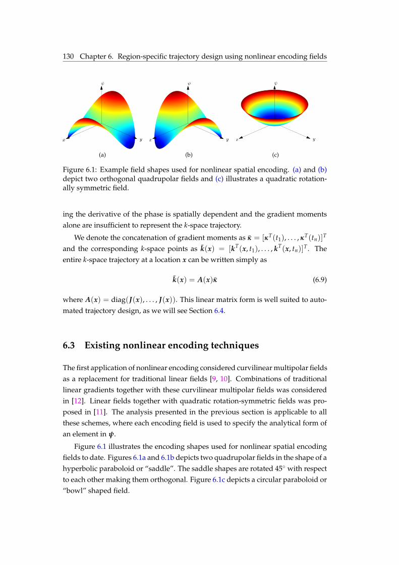
130 Chapter 6. Region-specific trajectory design using nonlinear encoding fields
(a) (b) (c)
Figure 6.1: Example field shapes used for nonlinear spatial encoding. (a)(a) and (b)(b)depict two orthogonal quadrupolar fields and (c)(c) illustrates a quadratic rotation-ally symmetric field.
ing the derivative of the phase is spatially dependent and the gradient momentsalone are insufficient to represent the k-space trajectory.
We denote the concatenation of gradient moments as κ = [κT(t1), . . . , κT(tn)]T
and the corresponding k-space points as k(x) = [kT(x, t1), . . . , kT(x, tn)]T. Theentire k-space trajectory at a location x can be written simply as
k(x) = A(x)κ (6.9)
where A(x) = diag(J(x), . . . , J(x)). This linear matrix form is well suited to auto-mated trajectory design, as we will see Section 6.46.4.
6.3 Existing nonlinear encoding techniques
The first application of nonlinear encoding considered curvilinear multipolar fieldsas a replacement for traditional linear fields [99, 1010]. Combinations of traditionallinear gradients together with these curvilinear multipolar fields was consideredin [1212]. Linear fields together with quadratic rotation-symmetric fields was pro-posed in [1111]. The analysis presented in the previous section is applicable to allthese schemes, where each encoding field is used to specify the analytical form ofan element in ψ.
Figure 6.16.1 illustrates the encoding shapes used for nonlinear spatial encodingfields to date. Figures 6.1a6.1a and 6.1b6.1b depicts two quadrupolar fields in the shape of ahyperbolic paraboloid or “saddle”. The saddle shapes are rotated 45 with respectto each other making them orthogonal. Figure 6.1c6.1c depicts a circular paraboloid or“bowl” shaped field.

6.3. Existing nonlinear encoding techniques 131
6.3.1 Cartesian PatLoc
Perhaps the simplest application of nonlinear spatial encoding is known as Carte-sian PatLoc. In this technique, the linear phase encoding and readout gradientsof a simple Cartesian trajectory are replaced with the quadrupolar fields in Fig-ures 6.1a6.1a and 6.1b6.1b. In the ideal case, these fields can be described by scaling thespherical harmonics. Specifically,
ψa(x) = x2 − y2; ψb(x) = 2xy (6.10)
The vector of field shapes is
ψ(x) =
[x2 − y2
2xy
](6.11)
Since the gradients of the fields are orthogonal at all points (∇ψa · ∇ψb = 0), thetwo fields can be used for frequency and phase encoding, analogous to encod-ing with linear fields. Specifically, the trajectory, κ(t), is given by the Cartesiansequence diagram described in Section 3.5.13.5.1. A detailed analysis of this imagingstrategy will be provided in Chapter 77. In the present discussion we look at someof the basic properties of this scheme.
Simulated data was generated from a checkerboard phantom using a Carte-sian trajectory with 64 phase encode and 64 readout points. Reconstruction wasperformed using the conjugate gradient algorithm described in Section 3.63.6. Twoschemes were simulated: a traditional setup using two linear gradients and thePatLoc setup with orthogonal quadrupolar fields replacing the phase encode andreadout gradients. To visualise the spatial dependence of the encoding, the localk-space trajectory was calculated at points on a 5× 5 grid over the field of view.
Figure 6.26.2 displays the local k-space plots alongside the reconstruction results.Figure 6.2a6.2a displays the local k-space trajectory when linear encoding gradientsare used. In this case, the local k-space reduces to traditional notion of k-spaceand the square sampling pattern characteristic of a Cartesian trajectory is showneverywhere. Figure 6.2b6.2b displays the corresponding reconstruction demonstratinguniform resolution. Figure 6.2c6.2c depicts the local k-space for a Cartesian trajectoryusing the quadrupolar fields in (6.106.10). The spatial dependence of the local k-spaceis evident with a singularity in the center where the gradient of the fields is zeroand extended coverage at the periphery where the gradient is larger than the linearfields. Figure 6.2d6.2d display the corresponding image reconstruction which demon-strates spatially varying resolution. In the center, the resolution is poor with pro-

132 Chapter 6. Region-specific trajectory design using nonlinear encoding fields
(a) (b)
(c) (d)
Figure 6.2: Example of a Cartesian trajectory with nonlinear encoding fields. Thelocal k-space is depicted in (a)(a) for linear fields and (c)(c) for quadrupolar PatLocfields. Reconstructions of a simulated checkerboard phantom are shown in (b)(b)and (d)(d).
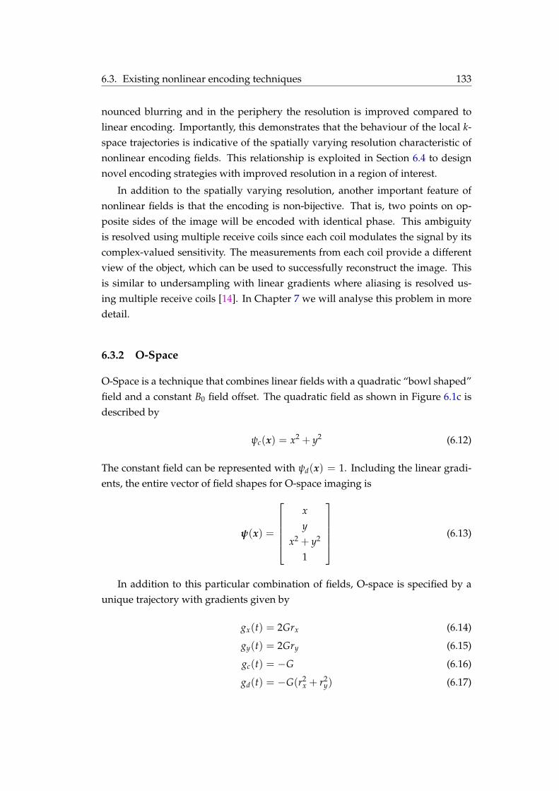
6.3. Existing nonlinear encoding techniques 133
nounced blurring and in the periphery the resolution is improved compared tolinear encoding. Importantly, this demonstrates that the behaviour of the local k-space trajectories is indicative of the spatially varying resolution characteristic ofnonlinear encoding fields. This relationship is exploited in Section 6.46.4 to designnovel encoding strategies with improved resolution in a region of interest.
In addition to the spatially varying resolution, another important feature ofnonlinear fields is that the encoding is non-bijective. That is, two points on op-posite sides of the image will be encoded with identical phase. This ambiguityis resolved using multiple receive coils since each coil modulates the signal by itscomplex-valued sensitivity. The measurements from each coil provide a differentview of the object, which can be used to successfully reconstruct the image. Thisis similar to undersampling with linear gradients where aliasing is resolved us-ing multiple receive coils [1414]. In Chapter 77 we will analyse this problem in moredetail.
6.3.2 O-Space
O-Space is a technique that combines linear fields with a quadratic “bowl shaped”field and a constant B0 field offset. The quadratic field as shown in Figure 6.1c6.1c isdescribed by
ψc(x) = x2 + y2 (6.12)
The constant field can be represented with ψd(x) = 1. Including the linear gradi-ents, the entire vector of field shapes for O-space imaging is
ψ(x) =
xy
x2 + y2
1
(6.13)
In addition to this particular combination of fields, O-space is specified by aunique trajectory with gradients given by
gx(t) = 2Grx (6.14)
gy(t) = 2Gry (6.15)
gc(t) = −G (6.16)
gd(t) = −G(r2x + r2
y) (6.17)

134 Chapter 6. Region-specific trajectory design using nonlinear encoding fields
where rx and ry parameterise the projection11. Different projections are acquired byaltering the values of rx and ry. The entire acquisition can be specified by a set ofvectors, rq = (r(q)x , r(q)y ) for q = 1, . . . , Ne. In this case, the encoding field in (6.46.4)becomes
b(x, t) = G‖x− rq‖2 (6.18)
It is evident that the role of the two linear gradients and the B0 offset is to shiftthe centre of the quadratic field. With this field shape, projections of the objectare obtained along rings expanding outward from the centre point, rq. Indeed, theterm ‘O-space’ was motivated by the circular isocontours of the encoding field. Bytranslating the centre point each projection, all regions obtain some spatial encod-ing and the central singularity in Cartesian PatLoc is avoided.
6.3.3 4D-RIO
Another technique, termed 4D-RIO, simultaneously employs two linear and twoquadrupolar fields for spatial encoding. The fields are specified by the vector,
ψ(x) =
xy
x2 − y2
2xy
(6.19)
The trajectory for this technique is based on two standard radial trajectories usedto drive the linear and quadratic coils. The trajectories are out-of-phase such thatthe gradient waveforms for the nonlinear channels are maximum at times whenthe linear gradients are minimum and vice versa.
6.4 Region specific trajectory design
As demonstrated above, an important consequence of nonlinear encoding fieldsis that the image resolution is spatially varying. The combination of linear andnonlinear encoding fields was examined in [1212] and it was demonstrated that dif-ferent trajectories produce different regions of improved and degraded resolution.A simple forward analysis was presented based on the concept of local k-space,where the resolution can be predicted for a given trajectory. We propose the op-posite; we design a multidimensional trajectory given the required resolution. In
1This is similar to angle parameterising a radial trajectory as discussed in Section 3.5.23.5.2.

6.4. Region specific trajectory design 135
this way, it is possible to design trajectories with improved resolution in a regionof interest.
We define an optimisation problem based on the local k-space trajectory at dif-ferent points within the region of interest. Numerical optimisation of gradientwaveforms has been previously proposed for linear encoding in a range of works,e.g. [9393] and references therein. In our case, the addition of nonlinear encodingmeans that no solution exists that implements our target trajectory at all locationswithin the desired region. Instead, we seek to minimise the difference betweenthe local k-space trajectories and the target trajectory. To increase the clarity of theproposed technique, our target trajectory is based on a simple EPI scheme with noramp-sampling, although more complex trajectories are possible.
To date, nonlinear spatial encoding has only been applied to projection imagingwith multiple excitation pulses. In addition to trajectory design, we demonstratethe first application of nonlinear encoding fields for single-shot imaging. Single-shot imaging is particularly well suited to multidimensional trajectories, wherethe additional encoding gradient channels can overcome the limitations associatedwith fast switching.
6.4.1 Trajectory optimisation
Similar to the global k-space trajectory for linear encoding, the sampling trajectoryof local k-space contains valuable information on properties of the reconstructedimage. In this work, we focus on resolution, as we aim to improve the resolution ina localised region. The global image resolution for linear encoding is determinedby the width of the main lobe of the point spread function, which is inversely pro-portional to the extent of the traditional k-space trajectory. Likewise, for nonlinearencoding, the resolution at a given position is determined by the extent of the localk-space trajectory at that position.
Based on k-space intuition, a trajectory that covers twice the maximum spatialfrequency will produce images with a two-fold improvement in resolution. Ad-ditionally, the trajectory should cover k-space with sufficient uniformity to ensurethe reconstruction is reasonably well conditioned. The assumption here is thatany undersampling resulting from an increased distance between k-space pointscan be resolved using multiple RF coils and the information from the associatedsensitivity maps.
This has close links to traditional parallel imaging where, for a fixed numberof measurements, k-space is undersampled so the maximum spatial frequency isgreater than that achievable by satisfying Nyquist limit. It is well known that this
136 Chapter 6. Region-specific trajectory design using nonlinear encoding fields
undersampling leads to aliasing which can be resolved using information from thecoil sensitivity profiles [1414, 9494]. In our case, a similar situation exists except thatwe aim to control the region where undersampling occurs.
We use the notion of local k-space to define an optimisation problem for tra-jectory design. Specifically, we define a target k-space trajectory for points insidethe region of interest and try to find the gradient moments to achieve this. Fora fixed readout time, conventional single-shot trajectories (such as EPI or spiral)using only linear gradients cover a maximum spatial frequency that is limited bygradient performance and safety considerations. As such, good candidates forthe target trajectory are single-shot trajectories that cover an increased spatial fre-quency. The aim is that additional nonlinear encoding channels can be used toextend the coverage of local k-space (at the expense of undersampling) to improvethe resolution in the desired region.
It is impractical to calculate the local k-space trajectory at every pixel in the re-gion of interest. Instead we calculate the trajectory at a set of control points withinthe region. Since the encoding fields are smooth, the local k-space trajectory willvary smoothly over the imaging region. Thus it is sufficient to specify the desiredtrajectory at a small number of points and find the gradient waveforms that ap-proximately achieve this while satisfying the physical constraints of the scannerhardware. It will be demonstrated in this work that the addition of nonlinear en-coding fields allows the calculation of gradient waveforms that steer the areas ofimproved resolution to the region of interest.
To formulate an optimisation problem we define the target k-space trajectory,ktar, as the concatenation of the target trajectories at each control point. Denotingthe set of control points by zii=1,...,p, the concatenation of the local trajectories ateach point is represented by the single matrix equation,
k = Aκ (6.20)
where
k =
k(z1)
...k(zp)
, A =
A(z1)
...A(zp)
. (6.21)
Ideally, we wish to find a set of gradient moments, κ, such that ktar = Aκ.In the general case, this is not always realisable due to the limited shapes of theencoding fields in ψ and the constraints imposed by safety considerations andhardware performance. Instead we seek to minimise the difference between the

6.4. Region specific trajectory design 137
desired trajectory and the actual trajectory, ‖ktar − Aκ‖, measured with a suitablenorm.
The physical constraints fall under two categories: equality constraints andinequality constraints. The equality constraints concern the initial and final statesof the gradient system. Specifically, the gradient waveforms must be zero at thestart and end of the sequence. It is also assumed that the system is in a resting stateprior to imaging, i.e. g(t) = 0 for t < 0, which means the initial gradient momentis also zero. The equality constraints are summarised as
g(t1) = 0, (6.22a)
g(tn) = 0, (6.22b)
κ(t1) = 0. (6.22c)
The inequality constraints deal with safety and hardware limitations concerningthe maximum gradient amplitude and the gradient slew rate. Constraints of thisform already exist in clinical scanners for linear gradients and the same constraintsshould be applied to additional nonlinear gradients. The gradient amplitude islimited by gmax and the slew rate by smax. These constraints can be written as
|g(t)| ≤ gmax , (6.23a)∣∣∣∣∂g(t)∂t
∣∣∣∣ ≤ smax . (6.23b)
The constraints in (6.226.22) and (6.236.23) are simple linear constraints and using finitedifference approximations for the time derivative, we can write them as Bκ = 0and Cκ ≤ b, respectively. In this work, we only constrain the switching rates ofindividual channels. In future work we plan to adapt the framework to considerthe effect of all channels simultaneously.
We can now define the optimisation as
minimise ‖ktar − Aκ‖subject to Bκ = 0
Cκ ≤ b.
(6.24)
Once the achievable gradient moments are found, the optimal gradient wave-forms are computed using finite differences to generate a waveform suitable forimplementation on the scanner.
Although the optimisation problem in (6.246.24) forms the basis of our trajectorydesign it is not directly applicable for our hardware. The scanner used in this study

138 Chapter 6. Region-specific trajectory design using nonlinear encoding fields
(see “experimental setup” below) requires a gradient waveform sampled every10 µs, known as the gradient raster time. However the ADC can acquire samplesfaster. In our phantom experiments, we set the ADC sampling time to 2.5 µs, sofour data samples are acquired for each gradient raster. Consequently, four localk-space points are also defined every gradient sample. To apply the optimisation,the gradient waveform (or gradient moment) must be related to the local k-space,which is achieved using an up-sampling matrix, U. We define U based on linearinterpolation. For example, an up-sampling matrix by a factor of two is,
U =
0.51
0.5 0.51
0.5. . .
⊗ Iq (6.25)
where ⊗ is the Kronecker product and Iq is the q× q identity matrix representingthe q encoding channels that require up-sampling.
Another consideration for EPI-based trajectories is the end-of-line transitiontime. This extra time after each acquisition line allows the gradient system tochange polarity. Our goal is to design a gradient waveform, g(t), for the entiretrajectory, ensuring the constraints are satisfied at each time point. However, ourobjective is to match only the appropriate portion of the trajectory to the targetk-space. We solve these differing requirements by seeking a complete trajectoryusing a cost function dependent only on the ‘central’ portion. This is implementedusing a rectangular selection matrix, S, which reduces the entire trajectory to thecentral part relevant for optimisation. Specifically,
S =
0 Irow 0 0 0 00 0 0 Irow 0 00 0 0 0 0 Irow
. . .
⊗ Iq (6.26)
where Irow is an identity matrix selecting a single row of the trajectory, the firstcolumn of zeros discards the prephase and subsequent zero columns discard theend-of-line transitions. Figure 6.36.3 illustrates the various waveform vectors and thematrices relating them.
Inclusion of the up-sampling and selection matrices defined in (6.256.25) and (6.266.26),
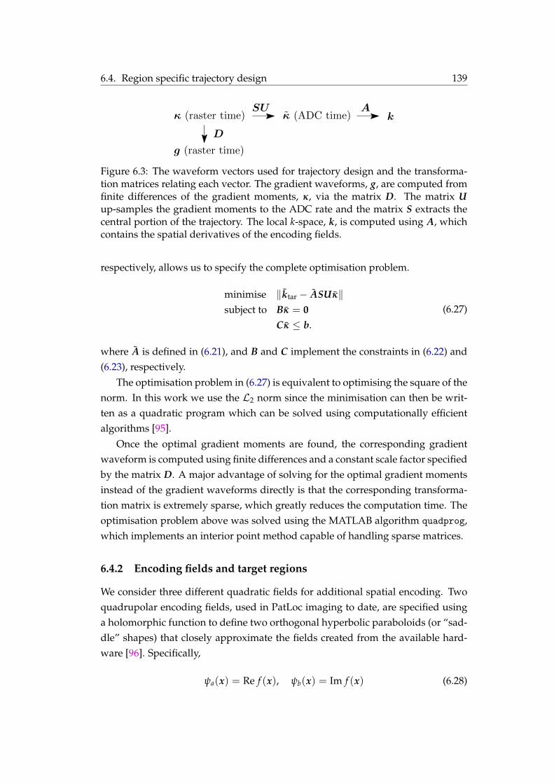
6.4. Region specific trajectory design 139
κ (raster time)
g (raster time)
D
SUκ (ADC time)
Ak
Figure 6.3: The waveform vectors used for trajectory design and the transforma-tion matrices relating each vector. The gradient waveforms, g, are computed fromfinite differences of the gradient moments, κ, via the matrix D. The matrix Uup-samples the gradient moments to the ADC rate and the matrix S extracts thecentral portion of the trajectory. The local k-space, k, is computed using A, whichcontains the spatial derivatives of the encoding fields.
respectively, allows us to specify the complete optimisation problem.
minimise ‖ktar − ASUκ‖subject to Bκ = 0
Cκ ≤ b.
(6.27)
where A is defined in (6.216.21), and B and C implement the constraints in (6.226.22) and(6.236.23), respectively.
The optimisation problem in (6.276.27) is equivalent to optimising the square of thenorm. In this work we use the L2 norm since the minimisation can then be writ-ten as a quadratic program which can be solved using computationally efficientalgorithms [9595].
Once the optimal gradient moments are found, the corresponding gradientwaveform is computed using finite differences and a constant scale factor specifiedby the matrix D. A major advantage of solving for the optimal gradient momentsinstead of the gradient waveforms directly is that the corresponding transforma-tion matrix is extremely sparse, which greatly reduces the computation time. Theoptimisation problem above was solved using the MATLAB algorithm quadprog,which implements an interior point method capable of handling sparse matrices.
6.4.2 Encoding fields and target regions
We consider three different quadratic fields for additional spatial encoding. Twoquadrupolar encoding fields, used in PatLoc imaging to date, are specified usinga holomorphic function to define two orthogonal hyperbolic paraboloids (or “sad-dle” shapes) that closely approximate the fields created from the available hard-ware [9696]. Specifically,
ψa(x) = Re f (x), ψb(x) = Im f (x) (6.28)

140 Chapter 6. Region-specific trajectory design using nonlinear encoding fields
x
y
FOV
z2z1
L
(0, 0)
(L2 ,L2 )
ROI
(a)
x
y
FOV
z2
140
z1
L
(0, 0)
(L2 ,L2 )ROI
(b)
ky
kmaxkmin
kmax
kmin
(c)
Figure 6.4: Field-of-view (FOV), region of interest (ROI) and control points (z1,z2) for (a)(a) the 3-component trajectory and (b)(b) the 4-component trajectory. The lo-cal k-space trajectory at the control points is optimised with respect to the targettrajectory in (c)(c).
where f (x) = (x + iy)2e−iπ/4. The e−iπ/4 factor represents a 22.5 rotation fromthe main axis, consistent with the location of the physical coils. The third quadraticfield is a circular paraboloid (or “bowl” shaped), currently used in O-space imag-ing [1111], represented by the function
ψc(x) = x2 + y2. (6.29)
Although our site does not have hardware to generate this nonlinear encodingfield, other sites have reported on its performance, and therefore this field is stud-ied to demonstrate the generality and broader applicability of the present ap-proach.
With these analytical forms the multidimensional function, ψ, can by specifiedfor any combination of linear and nonlinear fields. Importantly, all physically-realisable fields satisfy Laplace’s equation thus the spatial derivatives are well-defined and the matrix J can be specified. We can then select the control points andtarget trajectory and solve the optimisation problem to generate the appropriategradient waveforms. In this work we consider two regimes illustrated in Fig. 6.46.4:
3-component: Linear & Circular Paraboloid, Right-Sided Enhancement In this setupwe use a combination of two linear gradients and a circular paraboloid fieldto enhance the resolution on the right side of the image. As illustrated inFig. 6.4a6.4a, the region of interest is defined using the control points,
z1 = (L/4, 0), z2 = (L/2, 0) (6.30)

6.4. Region specific trajectory design 141
where L is the field-of-view in both the x and y directions. The encodingfunction and its spatial derivative are
ψ(x) =[
x y x2 + y2]T
, J(x) =
[1 0 2x0 1 2y
]. (6.31)
4-component: Linear & Hyperbolic Paraboloid, Top-Left Enhancement In this regimewe use the two linear gradients and the two PatLoc quadrupolar fields totarget the top-left region of the image. The control points for this regime areshown in Fig. 6.4b6.4b. Specifically,
z1 = ((L/2) cos 140, (L/2) sin 140), z2 = ((L/4) cos 140, (L/4) sin 140).(6.32)
A 140 line of focus is selected to demonstrate the flexibility of the targetregion, beyond the regions naturally selected by the field geometry. The en-coding function and spatial derivative in this case are
ψ(x) =[
x y Re f (x) Im f (x)]T
, (6.33)
J(x) =
[1 0 Re ∂ f
∂x (x) Im ∂ f∂x (x)
0 1 Re ∂ f∂y (y) Im ∂ f
∂y (x)
](6.34)
where ∂ f∂x (x) = 2xe−iπ/4 and ∂ f
∂y (x) = 2ye−iπ/4.
In both regimes the target trajectory is a Cartesian EPI illustrated in Fig. 6.4c6.4c.For a fixed acquisition time, the maximum k-space position of a standard linear-gradient EPI, klin
max, is limited by the gradient and slew constraints. To improvethe resolution, we define the target trajectory to cover twice the maximum spatialfrequency of the linear-only EPI. That is, kmax = 2klin
max. This was chosen to obtainapproximately a two-fold improvement in resolution, based on k-space intuition.We consider slice-selective imaging, where the linear z-gradient is used to excite aslice and the remaining fields are used to encode the 2D image. Thus the trajectorynames ‘3-component’ and ‘4-component’ refer to the number of encoding channelsused to encode two spatial dimensions.
Each regime above specified the region of interest using two control points. Asingle control point creates a simpler optimisation problem although this results inresolution with a larger variation across the region of interest. On the other hand, itis possible to specify more than two control points; however, it was found that thisdid not greatly change the resulting trajectories, due to the fact that the encoding

142 Chapter 6. Region-specific trajectory design using nonlinear encoding fields
fields vary relatively slowly across space.In both cases the target trajectory consisted of 64 lines with 64 samples each
line. For safety considerations the maximum gradient, gmax, for the linear chan-nels was set to a conservative 22 mT/m. This is the minimum strength requiredto implement a standard EPI in the given time. The maximum gradient for thenonlinear channels was set to 115 mT/m2, which was conservatively chosen to be15% below the limits of our current hardware. The maximum slew rate, smax, wasset to 170 T/m/s for the linear channels and 772 T/m2/s for the nonlinear chan-nels, which leads to equivalent dB/dt at the edge of the field-of-view. To meetthe slew rate constraints, extra time must be allocated to allow the gradients tosafely change polarity after each line. We refer to this time as the ‘end-of-line tran-sition’. Additionally, a prephase time is needed to initially move the trajectoryfrom the centre of k-space to the corner of the acquisition grid. In these exper-iments a prephase time of 640 µs and end-of-line transition time of 360 µs wasallocated. These relatively long transition times were chosen to prevent ramp-sampling, which simplifies the presentation of our method. The total duration ofthe single-shot trajectories was 44.16 ms.
6.4.3 Simulations
All simulations were conducted using MATLAB (The Mathworks, Natick, MA).Given the trajectory, κopt, resulting from the optimisation, the corresponding localk-space at the point xi was computed using
k(xi) = A(xi)SUκopt. (6.35)
To visualise the local k-space over the entire field-of-view, a 5× 5 grid of locationswas defined and the local k-space of each location is plotted on an equivalent grid.
The local resolution of each trajectory was determined by calculating the widthof the point spread function (PSF). The PSF was approximated by back-projectingmeasurements simulated from a single source pixel (similar to calculating a row ofE′E where E is the encoding matrix). The accuracy of this approach was verifiedat eight points around the field of view by calculating the full PSF using conju-gate gradient reconstruction. Good quantitative agreement was found betweenour approximation and the full PSF. The width of the 2D PSF was quantified in thex and y directions by integrating the absolute value of the PSF along a horizontalor vertical line centred at the source pixel. Since the height of the PSF is indepen-dent of pixel location (neglecting coil sensitivities), the sum provides a measureof width. The maximum width over both directions was chosen as a measure of

6.4. Region specific trajectory design 143
resolution. This was repeated for each pixel to build a quantitative map of theresolution.
Simulated measurements were created from the designed trajectories using adiscrete approximation of the signal model in (6.16.1). The coil sensitivities of eightRF coils were simulated in the magnetostatic approximation of the Biot-Savart lawfor single coil loops arranged concentrically around the field-of-view. The encod-ing phase, φ, was calculated using the optimal trajectory and the encoding func-tion ψ defined analytically as the appropriate combination of linear fields (x, y)and quadratic fields (ψa, ψb, ψc given by (6.286.28) and (6.296.29)).
The magnetisation, m, was defined by a numerical phantom, which consistedof a checkerboard pattern multiplied by a circular mask and filtered using a Ham-ming window to remove the very high spatial frequencies. This phantom wasgenerated at a significantly higher resolution (512 × 512) compared to the finalreconstructed images (128× 128), to increase the accuracy of the discrete approx-imation used to simulate the integral in (6.16.1). Finally, independent complex noisewas added with zero mean and a standard deviation equal to 5% of the mean sig-nal intensity, identical to previous studies [1212]. Images were reconstructed usingthe iterative conjugate-gradient method described in Section 3.63.6.
6.4.4 Experiments
In vivo and phantom experiments were conducted on a 3 T clinical imaging sys-tem (MAGNETOM, Trio Tim, Siemens Healthcare, Erlangen, Germany) fitted witha custom-built gradient insert-coil. The insert-coil generates two fields which ap-proximate a hyperbolic paraboloid where one field is rotated 45 with respect tothe other to create two orthogonal encoding fields. These encoding fields havebeen previously described in [9797].
The coils for each quadrupolar field can be driven with currents up to 80 Ausing additional high-performance gradient amplifiers. The scanner architecturewas modified to control both the linear gradient coils and the PatLoc gradient coils,which allows us to simultaneously and independently drive the five encoding gra-dients. A Siemens head coil, used in the PET-MR scanner, was fitted inside the gra-dient insert and contained a single RF coil used for excitation and an eight channelcoil array for receiving.
This hardware cannot generate a circular paraboloid shaped field so only the 4-component regime is tested experimentally. Thus after the slice selection gradient,the remaining two linear and two quadrupolar fields are driven simultaneously toencode the two dimensional slice. To achieve this, an existing MRI sequence for

144 Chapter 6. Region-specific trajectory design using nonlinear encoding fields
single-shot three-dimensional encoding was modified for our purposes. Impor-tantly, the sequence allows us to specify arbitrary gradient waveforms for each ofthe five encoding channels.
The phantom used in experiments is a 190 mm diameter plastic cylinder con-taining approximately 130 thin Plexiglas tubes (with diameter ∼4 mm) parallel tothe longitudinal axis of the cylinder. The cylinder and tubes were filled with waterdoped with nickel sulfate and sodium chloride to give suitable contrast.
All acquisitions had a field-of-view of 220 mm and images were reconstructedto a 128× 128 grid using the conjugate gradient algorithm described in Section 3.63.6.The trajectories had an effective TE ≈ 21.8 ms, which is half the readout duration.A single ADC event was used throughout the single-shot readout, all samples ofwhich were included in the image reconstruction. The data were sampled withan ADC dwell time of 2.5 µs and 5 µs for the phantom and in vivo experiments,respectively. The ADC sampling rate must be high enough to capture the largestpossible phase change between consecutive readout points. If the sampling rate istoo low, the local frequency may be outside the acquisition bandwidth and the sig-nal from these regions will be attenuated by the scanner’s anti-aliasing filter. Theslice thickness was 2 mm for phantom experiments and 3 mm for in vivo experi-ments. Thin slices were chosen to minimise signal dropouts due to through-planedephasing [9898].
6.4.5 Calibration
As the single-shot trajectories become shorter and the hardware limits of the gra-dient coils are approached, the actual trajectory can deviate significantly from thedesired trajectory [9999]. These deviations originate from many sources includingeddy currents, thermal drifts, hardware delays and concomitant fields. Withoutadequate correction, these inaccuracies can cause blurring, geometric distortionsor ghosting in reconstructed images [100100]. The problems have been partially ad-dressed by characterising the eddy-currents [101101], measuring the k-space trajectory[9999] and by correcting for distortions due to concomitant fields [102102]. In recentyears, the magnetic field has been monitored by measuring the signal from fieldprobes [103103, 104104, 105105, 106106, 107107, 108108] and fitting the signal phase to a model of thefield evolution. This paradigm was used to successfully reconstruct images frome.g. spiral trajectories [104104, 106106] or echo-planar imaging [106106] in the presence ofundesirable field perturbations. In [108108], the field evolution was modelled by realsolid harmonics up to third order to account for higher order field perturbationsin diffusion imaging. In this work where a custom-built nonlinear gradient coil

6.4. Region specific trajectory design 145
insert is used, the problem of gradient field deviations is even more pronounced.In order to calibrate the simultaneously applied gradient waveforms from the lin-ear and the nonlinear gradient coils, a field camera with 16 field probes is used[105105, 108108, 109109].
Reconstruction of the experimental data requires accurate estimates of the RFsensitivity maps cl(·), trajectory κ(·) and gradient shapes ψ(·). In this work wemeasure the effective trajectories using a ‘field camera’ constructed with 16 1Hfield probes [105105, 106106, 108108]. The field probes were placed approximately equidis-tant around the surface of a sphere with a radius of 9 cm. The probes were excitedusing a separate transmit chain, similar to [110110], consisting of a signal generator(N5181A, Agilent, Santa Clara, CA, USA), a power amplifier (75A400, AmplifierResearch, Souderton, PA, USA) and a power splitter (MITEQ-ESTONIA, Estonia).The separate transmit chain was controlled via the optical trigger from the scan-ner. The inserted RF coil and the eight channel head coil array were kept in thegradient coil and connected to a coil test-bench for detuning and grounding dur-ing the trajectory calibration measurements. The field probes were excited with arectangular RF pulse of 5 µs duration and the resulting signal was sampled withan ADC dwell time of 2.5 µs. This setup is based on work in [105105, 108108, 110110] and hasbeen previously used in [109109] to characterise the PatLoc gradients.
The encoding phase evolution was modelled with 16 real valued spherical har-monics up to 3rd order. The 16 basis functions define the vector of field shapesψ. The 16 corresponding coefficients were fit to the probe measurements using astandard least squares algorithm [106106] to define the trajectory κ (referred to as the‘measured trajectory’). In this way we obtain a very accurate estimate of the actualencoding phase at each time point. With our current hardware setup we measuredthe trajectory in a separate scan.
For comparison purposes, we also reconstructed images using the ‘nominaltrajectory’ and encoding field shapes obtained using data from a custom 8 echoGRE sequence (128× 128, 5 mm slice thickness, 220 mm field-of-view, 4 ms echospacing) used previously in [111111]. The field mapping was performed on the im-aged object immediately prior to acquisition. The nominal trajectory was obtainedby adding a 0.6 µs delay to the linear channels and a 5.3 µs delay to the nonlinearchannels of the optimised trajectory. The time delays were estimated empiricallyin order to reconstruct the best possible image. For both the measured and nomi-nal reconstructions, the RF sensitivities were estimated using an adaptive methodbased on a stochastic formulation of the matched filter, as in [112112], with data fromthe first echo of the field mapping sequence.

146 Chapter 6. Region-specific trajectory design using nonlinear encoding fields
6.4.6 Safety considerations
In vivo experiments were performed on a healthy volunteer after suitable IRB ap-proval was obtained. Since this was the first application of single-shot imagingusing linear and nonlinear fields simultaneously, it was important to address po-tential safety issues. The safety of the gradient-insert coil for traditional PatLocimaging has been described in [113113]. The implementation of single-shot imagingbrings an increased risk of peripheral nerve stimulation (PNS) due to the rapidlyswitching linear and nonlinear gradients. To mitigate the risk the gradient wave-forms were initially implemented at 40% of the desired strength, which reducesthe slew rates by the same factor [114114]. This ensured the maximum magnitude ofdB/dt was below 20 T/s throughout the region covering the subject’s body. Theamplitudes were then increased in 10% increments, each time confirming with thevolunteer that no PNS was experienced.
A further safety consideration was the elevated acoustic noise generated fromthe custom gradient-insert. Previous experiments in [113113, 114114] reported a soundpressure level (SPL) above regulatory guidelines for a gradient switching frequencybetween 480–650 Hz. A Fourier analysis of the optimised trajectories in this chap-ter indicated a dominant frequency of ∼750 Hz, well above the problematic fre-quencies. After measuring the SPL of the sequence with a calibrated microphone,the risk of auditory damage was deemed negligible with the use of suitable earplugs.
6.5 Results
6.5.1 Trajectory optimisation and simulations
The gradient waveforms for the 3-component and 4-component encoding schemeswere calculated from the optimisation procedure described above. Figure 6.56.5 dis-plays the 3-component and 4-component gradient waveforms necessary to en-hance the desired regions of the image. Since the target trajectory is an under-sampled EPI trajectory (Fig. 6.4c6.4c), the waveforms are similar to a conventional EPIsequence. Most noticeable are the constant gradients during readout lines andblips of gy between lines.
The local k-space trajectories for the linear, 3-component and 4-component en-coding regimes are plotted in Fig. 6.66.6, together with the simulation results. Thelocal k-space trajectories in Figs. 6.6d6.6d and 6.6g6.6g appear ‘skewed’ and are not exactlyequal to the target trajectory in the desired regions due to the gradient constraintsand nonlinear encoding fields. However, the optimised local k-space trajectoriesretain the desired features: the samples are regularly spaced and have increased

6.5. Results 147
0.5 1 1.5 2 2.5
0
1
ADC
time (ms)
−20
0
20
gx
−1
0
1
gy
−100
0
100
gc
(a)
0.5 1 1.5 2 2.5
0
1
ADC
time (ms)
−200
20
gx
−202
gy
−200
20
ga
−1000
100
gb
(b)
Figure 6.5: The gradient waveforms using (a)(a) 3-component encoding with twolinear and one quadratic and (b)(b) 4-component encoding using two linear and twoquadrupolar fields. The linear waveforms (gx, gy) are in units of mT/m whereasthe nonlinear waveforms (ga, gb, gc) are in units of mT/m2 reflecting the quadraticnature of the corresponding fields over the spatial dimension. The plots displaythe first few milliseconds after the pre-phasing.
coverage. The fine details of the checkerboard phantom are completely blurredout for conventional linear encoding as shown in Fig. 6.6c6.6c. The blurring occurs be-cause the hardware and safety constraints imposed for single-shot imaging limitthe k-space extent achievable in a fixed acquisition time. The addition of extranonlinear encoding channels allows us to increase the boundaries of the local k-space trajectory in the regions we are interested in, effectively increasing the reso-lution in those parts of the image. This is demonstrated in the simulation resultsof Figs. 6.6f6.6f and 6.6i6.6i where the checkerboard details can be shown in the desiredregions, i.e., the right side for the 3-component encoding and top-left corner forthe 4-component encoding scheme.
Some intuition about the gradient waveforms resulting from the optimisationcan be gained by considering the local k-space equation. For example, the k-spacefor the 3-component trajectory is given by,
k(x, t) =
[kx(x, t)ky(x, t)
]=
[κx(t) + κc(t)xκy(t) + κc(t)y
]. (6.36)
During a readout line we must move the x-coordinate of the local k-space trajec-tory from −kmax to kmax in a relatively short time. Once the linear channel, κx(t),is at maximum strength the additional term of κc(t)x is crucial. The right side ofthe image is represented by x > 0, thus to enhance the k-space coverage in this re-

148 Chapter 6. Region-specific trajectory design using nonlinear encoding fields
(a)
0
0.1
0.2
0.3
0.4
0.5
0.6
0.7
0.8
0.9
1
(b) (c)
(d)
0
0.1
0.2
0.3
0.4
0.5
0.6
0.7
0.8
0.9
1
(e) (f)
(g)
0
0.1
0.2
0.3
0.4
0.5
0.6
0.7
0.8
0.9
1
(h) (i)
Figure 6.6: The (left) local k-space, (middle) estimated PSF width and (right) simu-lated reconstructions of a numerical checkerboard phantom for different gradientwaveforms. The linear, 3-component and 4-component encoding schemes are pre-sented in the top, middle and bottom rows, respectively.

6.5. Results 149
gion we require positive values of κc(t) during a left-to-right readout and negativevalues during a right-to-left readout line. This explains why the correspondinggradient waveform gc(t) follows the waveform of the x-coordinate, gx(t). Thisanalysis also suggests that to enhance the left side of the image, we can simply flipthe quadratic channel waveform by applying −gc(t) instead.
More subtle behaviour is observed in the y-coordinate, ky(x, t). In this case, weare interested in the transition between readout lines and the appropriate gradientwaveforms to increment the trajectory by a small amount. The gradient waveformbetween the end of readout line, τ1 and the beginning of the next, τ2 is symmetricabout the time axis, so the corresponding gradient moment after this period iszero,
κc(t) =∫ τ2
τ1
gc(τ)dτ = 0. (6.37)
Thus ky(x, t) = κy(t) is only dependent on the y-gradient, which is not limitedby amplitude or switching constraints for our simple target trajectory. Similarly,the local k-space extent in the y direction is not a function of position, unlike thex direction described above.
Another interpretation of the results is available by noting that during the read-out the gradient waveforms of the additional channels are proportional to the lin-ear readout gradient. This means the ‘readout’ encoding fields (all fields except ψy)can be replaced by an effective field, which is a linear combination of the encodingfields. To elucidate this point we consider the 4-component gradient waveformsin Fig. 6.5b6.5b. During the readout periods the gradient moments are related by con-stants λ and η such that κa(t) = λκx(t) and κb(t) = ηκx(t). According to (6.76.7), thephase can be written as
φ(x, t) = κx(t) (ψx(x) + λψa(x) + ηψb(x))︸ ︷︷ ︸ψeff(x)
+κy(t)ψy(x). (6.38)
We see that, in this case, the 4-component encoding is equivalent to traditional2D encoding with a different readout field given by the effective encoding fieldψeff(x). Figure 6.76.7 illustrates the two effective encoding fields of the 4-componenttrajectory in Fig. 6.5b6.5b. The effective readout field in Fig. 6.7a6.7a has maximum gra-dient in the region of interest demonstrated by a narrow distance of neighbouringcontours and length of the arrows representing the spatial gradient. The gradientis also maximally orthogonal to the phase encoding gradient in Fig. 6.7b6.7b in theregion of interest.
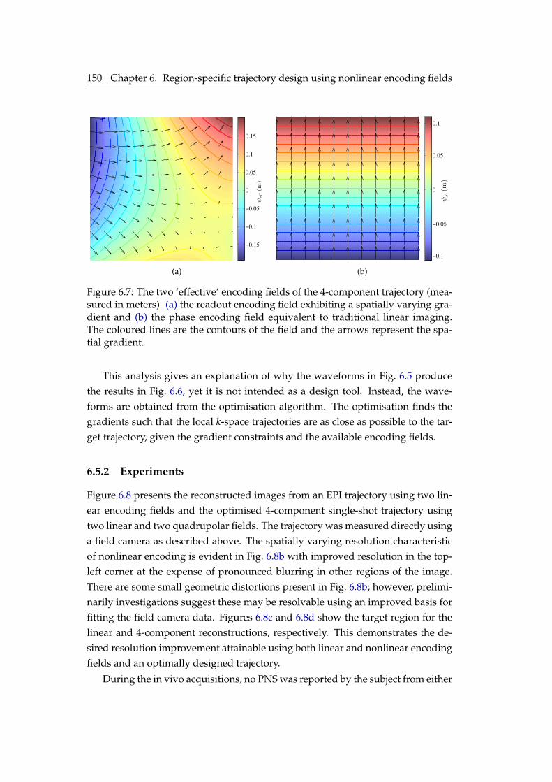
150 Chapter 6. Region-specific trajectory design using nonlinear encoding fields
−0.15
−0.1
−0.05
0
0.05
0.1
0.15
ψeff(m
)
(a)
−0.1
−0.05
0
0.05
0.1
ψy(m
)
(b)
Figure 6.7: The two ‘effective’ encoding fields of the 4-component trajectory (mea-sured in meters). (a)(a) the readout encoding field exhibiting a spatially varying gra-dient and (b)(b) the phase encoding field equivalent to traditional linear imaging.The coloured lines are the contours of the field and the arrows represent the spa-tial gradient.
This analysis gives an explanation of why the waveforms in Fig. 6.56.5 producethe results in Fig. 6.66.6, yet it is not intended as a design tool. Instead, the wave-forms are obtained from the optimisation algorithm. The optimisation finds thegradients such that the local k-space trajectories are as close as possible to the tar-get trajectory, given the gradient constraints and the available encoding fields.
6.5.2 Experiments
Figure 6.86.8 presents the reconstructed images from an EPI trajectory using two lin-ear encoding fields and the optimised 4-component single-shot trajectory usingtwo linear and two quadrupolar fields. The trajectory was measured directly usinga field camera as described above. The spatially varying resolution characteristicof nonlinear encoding is evident in Fig. 6.8b6.8b with improved resolution in the top-left corner at the expense of pronounced blurring in other regions of the image.There are some small geometric distortions present in Fig. 6.8b6.8b; however, prelimi-narily investigations suggest these may be resolvable using an improved basis forfitting the field camera data. Figures 6.8c6.8c and 6.8d6.8d show the target region for thelinear and 4-component reconstructions, respectively. This demonstrates the de-sired resolution improvement attainable using both linear and nonlinear encodingfields and an optimally designed trajectory.
During the in vivo acquisitions, no PNS was reported by the subject from either

6.5. Results 151
(a) (b)
(c) (d)
Figure 6.8: Reconstructions of a phantom experiment from (a)(a) the linear EPI trajec-tory and (b)(b) the optimised 4-component single-shot trajectory. The 4-componenttrajectory has been designed to provide improved resolution in the top-left regionof the image. The target region is magnified in (c)(c) and (d)(d).

152 Chapter 6. Region-specific trajectory design using nonlinear encoding fields
the linear-only or 4-component trajectories. Figure 6.96.9 displays the in vivo images,acquired using linear EPI and the optimised 4-component trajectory. The recon-structed image from the 4-component trajectory has a spatially varying resolutionas predicted by the simulation results. As with the phantom images, the resolu-tion is visibly enhanced in the desired region (Fig. 6.9d6.9d) compared to a standardEPI using only linear gradients (Fig. 6.9c6.9c). All the in vivo and phantom imageshave little geometric distortion or ghosting due to accurate knowledge of the tra-jectories, which were measured using the field monitoring device. However, thereis a small checkerboard-like artifact present in the in-vivo image. This may be dueto small residual errors in the calibration data. The images acquired using the 4-component trajectory also exhibit an elevated noise level within the target region,which reflects the usual trade-off between resolution and SNR.
Figure 6.106.10 demonstrates the importance of using the field monitoring deviceto measure the trajectory. Figure 6.10a6.10a displays the 16 spherical harmonic coef-ficients used to define the encoding phase during the first 30 ms of the optimisedsingle-shot trajectory. For a comparable display, the coefficients are scaled to repre-sent the accumulated phase from each component at the edge of the field-of-view.As expected, the dominant components are the first order components x and y (κ1
and κ2, respectively) describing the linear gradients and the second order com-ponents xy and x2 − y2 (κ4 and κ8, respectively) representing the two hyperbolicparaboloid encoding fields. To illustrate an example of the differences betweenthe nominal 4-component and the measured 16-component trajectories, Fig. 6.10b6.10bshows the initial rows of the resulting local k-space trajectories calculated at thefirst optimisation control point, ( L
2 cos 140, L2 sin 140). The higher-order terms of
the 16-component trajectory lead to a significant difference between the measuredand nominal local k-space trajectories. In particular, the drift in the vertical direc-tion is visible after only 8 rows of the trajectory, and is significantly worse by theend of the readout. Figure 6.10c6.10c displays a reconstructed image from the in vivodata using the nominal 4-component trajectory. The difference between the nom-inal and actual trajectories leads to significant artifacts and geometric distortioncompared to Fig. 6.9b6.9b, which was reconstructed using the measured trajectories.
6.6 Discussion
We have developed a method for automated design of multidimensional single-shot trajectories that improves the imaging resolution in a region of interest. Theuse of additional encoding fields allowed us to overcome physical constraints con-cerning the rapid switching necessary for single-shot imaging.

6.6. Discussion 153
(a) (b)
(c) (d)
Figure 6.9: Reconstructions of a healthy brain from (a)(a) the linear EPI trajectoryand (b)(b) the optimised 4-component single-shot trajectory. The region of interest ismagnified in (c)(c) and (d)(d).

154 Chapter 6. Region-specific trajectory design using nonlinear encoding fields
−200
0
200
−200
0
200
−200
0
200
0 5 10 15 20 25 30
−200
0
200
t (ms)
κ0
κ1
κ2
κ3
κ4
κ5
κ6
κ7
κ8
κ9
κ10
κ11
κ12
κ13
κ14
κ15
(rad)
(rad)
(rad)
(rad)
(a)
−4 −2 0 2 4
1.4
1.5
1.6
1.7
1.8
1.9
klocalx (×103 rad/m)
kloca
ly
(×10
3rad/m
)
measured 16-componentnominal 4-component
(b) (c)
Figure 6.10: A comparison of the nominal and measured trajectories. (a)(a) the 16measured spherical harmonic coefficients, converted to the phase contributions (inradians) at a radius of L/2 from the centre; (b)(b) the first 8 rows of the local k-spacetrajectory at the first optimisation control point, z1, derived using the nominal4-component trajectory and the measured 16-component trajectory; (c)(c) the recon-struction of the in vivo data using the nominal 4-component trajectory, for com-parison with the measured trajectory reconstruction in Fig. 6.9b6.9b.

6.6. Discussion 155
The reconstructed images in this chapter have similarities to those presented inprevious PatLoc literature. Images from a traditional Cartesian PatLoc trajectoryusing two orthogonal quadrupolar fields exhibit improved resolution at the pe-riphery at the expense of pronounced blurring in the central region, where the lo-cal encoding gradient tends to zero [1010]. The “Dual Cartesian” trajectory presentedin [1212] shifts the blurred region by simultaneously applying linear and nonlineargradients. As required, the images presented in this chapter also exhibit regionswith improved and degraded resolution; however, their locations are chosen priorto trajectory design. It is important to note that the region of improved resolutioncan be steered to other areas of the field-of-view, beyond what was demonstratedabove. In general, improvement can be expected for any region towards the pe-riphery, where these particular nonlinear fields are known to provide resolutionenhancement.
The target trajectory used in this study was a simple EPI trajectory with a gen-erous end-of-line transition time. This produced simple waveforms and allowedan analytical analysis of the results. However, the optimisation technique couldalso be applied to an EPI trajectory with ramp-sampling, allowing for a muchshorter end-of-line transition [4040]. In this case, the optimisation will trade offbetween increasing local k-space extent and compensating for the non-uniformsampling under the ramp. Additionally, the phase encode blips are often slew-rate limited and thus, analogous to the readout, the optimisation would includegradient moments from the nonlinear channels during the blip. This is a topic offollow-up studies.
A 16-channel field camera was used to measure the actual encoding trajectory,including higher order terms, in order to account for hardware imperfections, con-comitant fields and eddy currents. A similar 16-channel field camera based on thesame field sensors was used in [108108] to minimise geometric distortion in diffusion-weighted images. In this work, where fast-switching trajectories drive both linearand nonlinear gradients, the field camera was necessary to prevent severe artifactsin the reconstructed images.
The design framework, based on the definition of local k-space, is applicable toany set of encoding fields. For example, the method can be applied when the an-alytical form of the encoding field shapes is not known or difficult to characterise,such as [115115]. In this general case, it is sufficient to find a suitable set of basis func-tions that can accurately approximate the field shapes. Once this basis is chosen,the spatial derivatives can be computed and the appropriate optimisation problemcan be defined.
The general trajectory design method proposed in this chapter is also applica-

156 Chapter 6. Region-specific trajectory design using nonlinear encoding fields
ble to imaging with multiple excitations. The simplest modification would be toalter the slew rate constraints such that they only apply during each readout pe-riod. Since there is sufficient time between echoes, we can build up the necessarygradient moment prior to the next readout. Another technique is to parameterisethe k-space trajectory to restrict the possible gradient moments, e.g. by the angledefining a spoke in a radial trajectory. This can be included in the optimisation sothat we solve for the set of parameters instead of the trajectory directly.
An important problem is the likelihood of peripheral nerve stimulation (PNS)of the designed trajectories. In principle, a global resolution improvement is possi-ble using a linear gradient coil insert and each channel could be switched indepen-dently to overcome the hardware constraints, as demonstrated in [116116]. However,large rapid field changes would be present across the entire volume, increasingthe risk of PNS [117117]. On the other hand, an optimised nonlinear field trajectorywould only apply large field changes over local regions, which may reduce therisk of nerve stimulation. Although we can prove that the time derivative of theBz field is reduced, a complete investigation of this proposition would require acomputational model for PNS risk including the influence of other switched fieldcomponents (Bx, By) on the entire body [4242]. The optimisation framework couldbe adapted to include such a model though this is beyond the scope of this thesis.Analysing this risk, however, will become increasingly important as the maximumgradient and slew rates are increased beyond the conservative values used in thiswork.
The spatially varying resolution characteristic of nonlinear encoding fields leadsto an additional spatial dependence on the SNR and a trade-off exists between thetwo quantities. Indeed, the reconstructed images exhibited an increased noise levelin regions with improved local resolution. It may be desirable in future work toinclude a noise metric, e.g. [118118], into the optimisation algorithm such that a trajec-tory could be designed satisfying both resolution and SNR requirements, althoughthe computational requirements may become prohibitive in this case.
The inherent resolution/SNR trade-off suggests the current framework is mostuseful for acquisition schemes limited primarily by resolution, such as single-shotimaging. As such, this technique is readily applicable to functional MRI studiesconcerning a particular anatomical region of the brain.
6.7 Conclusion
In this chapter, we have developed an automated procedure to create single-shotmultidimensional trajectories that improve the resolution in a region of interest.

6.7. Conclusion 157
The use of linear and nonlinear encoding fields creates an additional degree offreedom that is used to steer the local resolution improvement. We have validatedour technique in simulations as well as phantom and in vivo experiments for ahardware configuration consisting of two linear and two quadrupolar fields. Acustom-built field camera was used to measure the actual trajectories, which wasnecessary to minimise artifacts in the reconstructed images.


CHAPTER 7
Noise performance for imagingwith nonlinear encoding fields
Contents7.1 Introduction . . . . . . . . . . . . . . . . . . . . . . . . . . . . . . . . . 159159
7.1.1 Notation . . . . . . . . . . . . . . . . . . . . . . . . . . . . . . . 161161
7.2 Image reconstruction using frame theory . . . . . . . . . . . . . . . . 1621627.2.1 Review of frame theory . . . . . . . . . . . . . . . . . . . . . . 162162
7.3 Analysis of block-structured encoding schemes . . . . . . . . . . . . 1661667.3.1 Reconstruction variance . . . . . . . . . . . . . . . . . . . . . . 166166
7.3.2 SENSE imaging . . . . . . . . . . . . . . . . . . . . . . . . . . . 168168
7.3.3 PatLoc imaging . . . . . . . . . . . . . . . . . . . . . . . . . . . 172172
7.4 Analysis of arbitrary encoding schemes . . . . . . . . . . . . . . . . 1781787.4.1 Approximate reconstruction variance . . . . . . . . . . . . . . 179179
7.4.2 O-Space imaging . . . . . . . . . . . . . . . . . . . . . . . . . . 180180
7.5 Simulations . . . . . . . . . . . . . . . . . . . . . . . . . . . . . . . . . 1821827.5.1 Methods . . . . . . . . . . . . . . . . . . . . . . . . . . . . . . . 182182
7.5.2 Results . . . . . . . . . . . . . . . . . . . . . . . . . . . . . . . . 184184
7.6 Discussion . . . . . . . . . . . . . . . . . . . . . . . . . . . . . . . . . . 1871877.7 Conclusion . . . . . . . . . . . . . . . . . . . . . . . . . . . . . . . . . 190190Appendices . . . . . . . . . . . . . . . . . . . . . . . . . . . . . . . . . . . . 1911917.A Basis selection . . . . . . . . . . . . . . . . . . . . . . . . . . . . . . . . 191191
7.1 Introduction
NONLINEAR spatial encoding has the potential to improve current imagingtechnologies by removing the linearity constraint on the gradient coils. These
novel schemes require a characterisation of the imaging performance using quan-titative metrics for resolution and noise. The previous chapter focused on the spa-tially varying resolution inherent in encoding with nonlinear fields. In this chapter,
159

160 Chapter 7. Noise performance for imaging with nonlinear encoding fields
we examine the noise properties of images reconstructed from nonlinear spatialencoding schemes.
In principle, analysis of the linear reconstruction employed by nonlinear en-coding schemes is straightforward and the pixel covariance matrix is easily de-fined. The difficulty lies in computing this covariance for the large matrices asso-ciated with practical image resolutions. Fourier imaging and its variations possessa structure that can be exploited to simplify the computation. For example, thenoise performance for traditional parallel imaging techniques such as SENSE [1414]and GRAPPA [9494] has been well quantified, using the familiar g-factor [1414, 119119]. In[1010], it was shown that PatLoc is a generalisation of SENSE for nonlinear fields andthus inherits the analytical results concerning the SNR and g-factor, with a correc-tion for the nonlinear field. However, the computation is intractable for arbitraryencoding schemes, such as O-space, 4D-RIO, Null Space Imaging, and the opti-mised schemes of Chapter 66. This motivates the development of an approximatemetric. As the tractability of SENSE and PatLoc is due to the inherent structureof the encoding schemes, we categorise these schemes as “block-structured encod-ing schemes”. Although the term PatLoc can refer to class of imaging schemes (asin [1212]), in this chapter we use the term exclusively for the PatLoc scheme with aCartesian trajectory described in Section 6.3.16.3.1.
In this chapter, we present a natural unification of block-structured and arbi-trary encoding schemes by considering frames in the object space. Frame theoryhas primarily been used to analyse the windowed Fourier transform and wavelets.See [1313, 120120] for an introduction to this field. In the context of MRI, frames havebeen used to derive an SNR expression for schemes that use RF pulse encodingtechniques in conjunction with linear encoding gradients [121121]. Additionally, the“generalised point spread function” in [122122] is described by a frame operator, al-though this was not explicitly mentioned in the paper, using it to assess differentRF excitation schemes.
In this work, we apply the theory of frames to develop an analysis frameworkapplicable to any MRI encoding scheme. Imaging performance is often measuredby the image SNR, which ultimately depends on the variance of the reconstructedpixels. We derive an expression for the variance, which includes the previousresults for SENSE and PatLoc while offering a novel understanding. Further-more, we provide a viable means to analyse the performance of general encodingschemes which we demonstrate using O-space as a case study.
The chapter is organised as follows. In Section 7.27.2 we review frame theory inthe MRI context. In Section 7.37.3 we derive an expression for the pixel variance andapply it to the block-structured encoding schemes of SENSE and PatLoc to gain

7.1. Introduction 161
a novel perspective on these techniques. In Section 7.47.4 we use our framework toderive an approximation for the variance of the reconstructed pixels and apply itto O-space imaging. Finally, in Section 7.57.5 we demonstrate the wide applicabilityof our metric and present a quantitative comparison of PatLoc and O-space.
7.1.1 Notation
Table 7.17.1 lists the important symbols used in this chapter. Although the list isnot exhaustive, it includes the majority of quantities. Additional notation will beintroduced as it is required.
Table 7.1: Common notation used in Chapter 77
Symbol Quantity
Measurementsm Magnetisationyl,q,i Measurements indexed by coil, echo and time sampleNc, Ne, Nt Number of coils, excitations, time samplescl Coil sensitivityφq,i Encoding phase distributionψ Vector of field shapesβl,q,i Encoding functionb(x, t) Encoding magnetic field
Frame theoryf Function to reconstructΦj, Φj Frame elements, dual frame elementsA, B Frame boundsT, T Analysis operator (continuous and discrete)T∗, T ′ Synthesis operator (continuous and discrete)S, S Frame operator (continuous and discrete)F, F Reconstruction operator (continuous and discrete)χ, ξ, ζ Pixel bases
AnalysisDN Dirichlet kernelΓ Weight matrix to whiten noiseΣ Measurement covarianced Volumetric correction factorD Diagonal matrix of correction factorsC Coil sensitivity matrixF Fourier transformκ, κ Coil kernelsh(u, u′) Block structure kernelXn Variance approximation

162 Chapter 7. Noise performance for imaging with nonlinear encoding fields
7.2 Image reconstruction using frame theory
As described in Section 6.26.2, the general form of an acquired MRI signal is an in-tegral transform of the underlying magnetisation. Ignoring relaxation effects thesignal equation is
sl(t) =∫
m(x)cl(x)e−jφ(x,t)dx. (7.1)
where cl is the coil sensitivity of the lth coil, φ is the accumulated phase distributionand m is unknown magnetisation.
In general, the signal is acquired over a number of RF excitations, each of whichresets the phase distribution. Additionally, measurements are collected at discretetime points, denoted ti. We introduce the notation φq,i(x) which represents thephase distribution for the qth excitation and ith time point. The discrete measure-ments, denoted yl,q,i, can be viewed as inner products on the space of functions,
yl,q,i = 〈m, βl,q,i〉, (7.2)
where there is an index for each coil, l, echo, q, and time, i. The encoding functions,βl,q,i are given by
βl,q,i(x) = cl(x)ejφq,i(x). (7.3)
The reconstruction problem is to estimate the object, m(·), from a set of pro-jections yl,q,i. From this perspective, the reconstruction problem lends itself to aframe theoretic formulation. Frame theory provides a performance analysis andoptimal reconstruction algorithm for a function observed through a sequence ofprojections, exactly the situation constructed in MRI. This formulation underscoresthe idea that the MRI reconstruction problem exists within a broader mathemat-ical context. Such abstraction may lead to further advances in the field of imagereconstruction.
7.2.1 Review of frame theory
We proceed with a brief introduction to frame theory followed by a matrix formu-lation that is readily applied to the discretised objects used for MRI reconstruction.For a more rigourous and detailed account consult, for example, [1313].
Frame theory is concerned with functions, f , belonging to a Hilbert space, V .In the context of MRI, f is the unknown magnetisation and V is the space of phys-

7.2. Image reconstruction using frame theory 163
ically plausible magnetisation distributions.
By definition, a set of functions, Φjj∈I , in a space, V , defined over a countableset, I , is a frame if there exists constants, 0 < A ≤ B < ∞ such that for all f ∈ V ,
A‖ f ‖2 ≤ ∑j∈I|〈 f , Φj〉|2 ≤ B‖ f ‖2 (7.4)
where A and B are the lower and upper frame bounds, respectively. We refer to thefunctions Φjj∈I as frame elements. The frame bounds reflect the robustness ofthe frame elements to perturbations, e.g. additive random noise on the projections.If A = B = 1 and ‖Φj‖ = 1, ∀j ∈ I , then Φjj∈I is an orthonormal basis. Inthis sense, the frame elements can be thought of as a generalised basis. The setI can be infinite for theoretical analysis although it is typically finite for practicalapplications.
In most applications, we obtain measurements (or frame coefficients) of an un-known function via the analysis operator, T : V → CM where M is the number offrame elements. The operator is defined as
T f = 〈 f , Φj〉j∈I . (7.5)
Similarly, we define the synthesis operator T∗ : CM → V as
T∗yjj∈I = ∑j∈I
yjΦj(x), (7.6)
which transforms the sequence of coefficients, yjj∈I , into a function in V . Noticethat T∗ is the adjoint of T. The frame operator S : V → V is the composition,S = T∗ T or
(S f )(x) = ∑j∈I〈 f , Φj〉Φj. (7.7)
If the functions, Φjj∈I , form a frame by satisfying the frame condition in(7.47.4), we can reconstruct any function from a sequence of noiseless transform coef-ficients as
f = ∑j∈I〈 f , Φj〉Φj = ∑
j∈I〈 f , Φj〉Φj, (7.8)
where Φjj∈I is the dual frame with the functions given by
Φj = S−1Φj. (7.9)

164 Chapter 7. Noise performance for imaging with nonlinear encoding fields
The relationship in (7.87.8) is exact and valid as long as (7.47.4) is satisfied. Note theduality in (7.87.8) in the sense that either Φj or Φj can be used for decompositionwith the other used for reconstruction. Adopting the convention of measuringwith the frame elements, Φjj∈I , and reconstructing with the dual, we can use(7.87.8) to define the reconstruction operator, F : CM → V as the composition,
F = S−1 T∗. (7.10)
In MRI the unknown function is the object’s magnetisation, i.e. f = m andthe operator in (7.107.10) would be used to reconstruct the magnetisation, m, from asequence of measurements, yl,q,i. The theory informs us that if the frame el-ements satisfy the frame condition in (7.47.4) then reconstruction is possible usingthe dual frame. Hence, it is desirable to find a frame in the two or three di-mensional object space using encoding functions realisable in the magnetic reso-nance setting. For MRI it is useful to consider frame elements Φl,q,i indexed bycoil, echo, and time sample. The results above are readily applicable to theseframe elements by considering indices from the set of tuples, I = (l, q, i) ∈[1, . . . , Nc]× [1, . . . , Ne]× [1, . . . , Nt], where Nc, Ne and Nt denote the number ofcoils, echoes and time samples, respectively.
In practice, we can only acquire a finite number of measurements so recon-struction of an arbitrary continuous function is impossible. Consequently, we areforced to restrict the space of functions by discretising the unknown functions intopixels. For this purpose we select a pixel basis, χn(x)N
n=1, so the object can berepresented by a linear combination of the functions, χn(x). For example, imagescan be represented using a rectangular basis where χn(x) = rectW(x− xn) for pixelwidth W. Mathematically, the basis is used to define a subspace, U , representingthe space of allowable functions,
U =
f ∈ V : f (x) =
N
∑n=1
fnχn(x)
. (7.11)
In this space, the problem of reconstructing an arbitrary object is transformed tothe problem of estimating a set of coefficients, fn.
Since a function f ∈ U is entirely described by the coefficients, f1, . . . , fN , thesubspace U is isomorphic to CN . Therefore the analysis operator, T, acting onfunctions in U can be considered as a mapping from CN to CM and thus admits amatrix representation, T . The corresponding matrix has elements given by
T(l,q,i),n = 〈χn, Φl,q,i〉. (7.12)
7.2. Image reconstruction using frame theory 165
The synthesis operator in this subspace, T∗ : CM → U , also has a matrix represen-tation,
T∗n,(l,q,i) = 〈Φl,q,i, χn〉. (7.13)
This can be represented as T ′, where T ′ is the conjugate transpose of the T definedby (7.127.12).
The frame operator in the discrete subspace is S : U → U , defined by thecomposition S = T∗ T. Equivalently this operator is represented as a matrix,called the frame matrix, defined by the equation,
S = T ′T (7.14)
A common example is when T is a full-rank matrix with orthonormal columns(such as a DFT matrix). In this case, the inverse is given by T ′ and the framematrix S is equal to the identity matrix.
The reconstruction operator using the dual frame in (7.107.10) simplifies to theMoore-Penrose pseudoinverse of the discrete analysis operator, T ,
F = S−1T ′ = (T ′T)−1T ′. (7.15)
When we select the frame elements to be the encoding functions used in MRI,Φl,q,i = βl,q,i, the analysis matrix in (7.127.12) becomes the standard encoding matrix[1414],
E(l,q,i),n = 〈χn, βl,q,i〉 (7.16)
In this case the measurements yl,q,i correspond to the frame coefficients.
An interesting question, given little attention in the literature, is how to choosethe pixel basis, χnN
n=1. The pixel basis must satisfy two conflicting requirements;firstly, the basis should lead to simple computation of the frame matrix and itsinverse, and secondly the basis should be able to accurately approximate the truefunctions. The Dirac delta distribution is ubiquitous since it satisfies the require-ment of simple computation. A rectangular basis potentially better represents thefunctions. Appendix 7.A7.A compares the two choices and shows that the differencein the final reconstructions for Fourier encoding is O(N−5/2) where N is the num-ber of pixels. This confirms the common notion that Dirac distributions sufficientlyapproximate the functions if the pixel grid is fine enough.

166 Chapter 7. Noise performance for imaging with nonlinear encoding fields
7.3 Analysis of block-structured encoding schemes
The impact of stochastic noise in the measurements must be considered for prac-tical applications of the presented theory. In the frame literature, reconstructionusing the dual frame has been shown to give the minimum mean-square error(MMSE) estimate, with global performance given by the lower frame bound [120120].However, exact quantification in terms of the variance of each pixel is desirablefor MRI applications. In this section we relate the pixel-wise variance to the frameoperator and apply the theory to the block-structured encoding schemes of SENSEand PatLoc.
7.3.1 Reconstruction variance
The signal model in (7.27.2) is modified to include additive noise,
yl,q,i = 〈m, βl,q,i〉+ vl,q,i. (7.17)
A discretised object can be represented by the vector, f = [ f1, . . . , fN ]T, where the
elements are fn = 〈χn, m〉. We construct the vectors, y = [y1,1,1, . . . , yNc,Ne,Nt ]T and
v = [v1,1,1, . . . , vNc,Ne,Nt ]T so (7.177.17) can be written as the matrix equation,
y = E f + v. (7.18)
The noise is complex Gaussian distributed, v ∼ N (0, Σ) for a general covariancematrix Σ. The size of Σ is NcNeNt × NcNeNt.
We desire a frame operator that adequately models the covariance so we con-sider the general case where the frame elements are a linear combination of encod-ing functions,
Φl,q,i = ∑l′,q′,i′
Γ(l,q,i),(l′,q′,i′)βl′,q′,i′ . (7.19)
This leads to frame coefficients that are a linear combination of the MRI measure-ments. Let Γ be a matrix of weights with elements Γ(l,q,i),(l′,q′,i′); the coefficients canbe defined by the matrix equation, η = Γy, with
η ∼ N (ΓE f , ΓΣΓ′). (7.20)
The analysis operator is T = ΓE and recall the frame matrix is S = T ′T . Thereconstructed function coefficients are given by f = Fη, where F is the reconstruc-

7.3. Analysis of block-structured encoding schemes 167
tion operator in (7.157.15). The covariance, X, of the reconstructed coefficients is
X = FΓΣΓ′F ′ (7.21)
= (T ′T)−1T ′ΓΣΓ′T(T ′T)−1 (7.22)
Since Σ is a covariance matrix, it is conjugate symmetric and thus the followingdecomposition is well defined, Σ−1 = Σ−1/2Σ−1/2. The main result of this sectionis that selecting the set of weights to be
Γ(l,q,i),(l′,q′,i′) = [Σ−1/2](l,q,i),(l′,q′,i′) (7.23)
yields
X = S−1 (7.24)
This equation reveals the close link between the frame elements, frame operator,and the resulting covariance. Importantly, the relationship is applicable for anynoise covariance, by the appropriate selection of the weighting matrix.
When the condition in (7.237.23) is satisfied, the frame matrix can be written interms of the discretised encoding functions as
S = E′Σ−1E (7.25)
In terms of the matrix elements we have,
Sn,m = ∑l,q,i
∑l′,q′,i′〈βl,q,i, χn〉Σ−1
(l,q,i),(l′,q′,i′)〈χm, βl′,q′,i′〉. (7.26)
This process of transforming the measurements is the same as ‘noise whitening’ inlinear estimation theory [66].
For white noise, Σ = σ2I, and the pixel variance is a scalar multiple of thatobtained by adopting an identity weighting matrix. In this case, the frame ele-ments are simply the MRI encoding functions. For correlated noise, the selectionof transformation weights, ensures the frame operator captures the properties ofthe reconstruction covariance. This is useful to analyse the noise performance ofexisting parallel imaging schemes, where noise is correlated between receive chan-nels [1414].
In the remainder of this section we apply our analysis to the existing imagingschemes of SENSE and PatLoc. The analysis of SENSE confirms the well-knownresults concerning SNR and coil sensitivities. Our analysis of PatLoc demonstrates

168 Chapter 7. Noise performance for imaging with nonlinear encoding fields
its relationship to SENSE as described in [1010]. For both techniques we presentthe existing analysis reported in the literature and our analysis using frame the-ory. The intention here is to provide a novel perspective on the workings of theseschemes.
7.3.2 SENSE imaging
SENSE imaging is a type of Fourier imaging and thus there is a linear relationshipbetween the phase and position, φq,i(x) = −2πkq,i · x as described in Section 3.4.43.4.4.The main feature of SENSE is that the encoding functions include the sensitivitiesfrom multiple coils,
βl,q,i(x) = cl(x)ej2πkq,i ·x. (7.27)
The quantity kq,i defines the position in spatial frequency space, k-space, as de-scribed in Section 3.4.43.4.4. Measurements are collected for a set of k-space coordinates(the trajectory), parameterised by time sample i and excitation number q. The gra-dients are changed after each excitation, defining the direction of the line throughk-space, which is then traversed as time evolves.
For faster acquisition, one can undersample by integer factors Rx and Ry inthe x and y directions, respectively. This reduces the number of measurementsby a factor of R = RxRy. Practically, only undersampling in the phase directionis useful to reduce imaging time since the sampling time in the readout directionis negligible. Nonetheless, our analysis is kept general to cover the case of 3DFourier imaging with two phase encode directions [123123]. We collect Nk = NtNe
measurements per coil with Nt = Nx/Rx, Ne = Ny/Ry. Given a field-of-viewof Lx × Ly, the maximum frequency, kmax
x = Nx/Lx, kmaxy = Ny/Ly is unchanged
by the undersampling, indicating the fundamental resolution is not affected. Themeasurements are collected at frequency points, kq,i = (i∆x, q∆y) where ∆x =
Rx∆x = Rx/Lx and likewise ∆y = Ry∆y.
7.3.2.1 Existing analysis of SENSE
The standard SENSE analysis originally presented in [1414] proceeds by adoptingthe delta distribution as the pixel basis and analysing the corresponding matrixequation for the measurement vector. Identical to (7.187.18) we have,
y = E f + v (7.28)

7.3. Analysis of block-structured encoding schemes 169
where v ∼ N (0, Σ) and E(l,q,i),n = cl(xn)e−j2πkq,i ·xn . The optimal reconstructionmatrix was proved to be [1414]
F = (E′Σ−1E)−1E′Σ−1. (7.29)
It is observed that for a given pixel centred at xp = (xp, yp), the group of aliasedpixels due to undersampling is given by the set,
Pp =(xp + nLx/Rx, yp + mLy/Ry) :
n ∈ [0, . . . , Rx − 1], m ∈ [0, . . . , Ry − 1] (7.30)
The problem of reconstruction is reduced to resolving this small set of pixels.We denote the R× 1 vector of coefficients for the aliased pixels as f (p). After per-forming an inverse DFT, this group of aliased pixels are related by
η = C(p) f (p) (7.31)
where C(p) is an Nc × R matrix with elements C(p)ln = cl(xn). The folding matrix,
C(p), highlights the crucial role of the coil sensitivities in successfully estimatingthe function coefficients. This structure is also revealed in the calculation of thereconstruction covariance matrix,
X = FΣF ′ (7.32)
=1
NtNe(E′Σ−1E)−1 (7.33)
Exploiting the block structure of E and Σ [1414], the noise matrix can be defined foreach group of aliased pixels,
X(p) =1
NtNe(C(p)′Σ(p)−1
C(p))−1 (7.34)
which involves the inversion of a small R× R matrix. The well-known g-factor isderived by considering the ratio of SNRs for the reduced and full acquisitions. Apixel is now indexed as (r, p) indicating the pixel and aliased group, respectively.For notational simplicity, the superscript (p) is dropped in the following g-factorequations. For full acquisition the covariance is denoted X and Nt = Nx, Ne = Ny.

170 Chapter 7. Noise performance for imaging with nonlinear encoding fields
Assuming that the signal strength is constant,
SNRfullr,p
SNRredr,p
=
√Xr,r√Xr,r
=√
R
√[(C′Σ−1C)−1]r,r√[(C′Σ−1C)−1]r,r
(7.35)
The case of full Fourier encoding yields a C that is an Nc × 1 column vector. Inthis situation there is no aliasing so our blocks contain only a single pixel and C isidentical to the nth column of the C matrix. Thus,
1Xr,r
= [C′Σ−1C]r,r (7.36)
Finally, the ratio of SNRs is expressed as
SNRfullr,p
SNRredr,p
=√
R√[C′Σ−1C]r,r[(C′Σ−1C)−1]r,r (7.37)
From this, the g-factor is defined as
gr,p =√[C′Σ−1C]r,r[(C′Σ−1C)−1]r,r (7.38)
Recall C and Σ are indexed by the aliased block, p, and the pair (r, p) is needed toindex a pixel.
7.3.2.2 Frame analysis of SENSE
The g-factor analysis above emerges naturally from the frame matrix, which em-phasises the source of the block structure. Central to this analysis is the periodicsinc, also known as the Dirichlet kernel, DN(x), defined as
DN(x) :=(N−1)/2
∑k=−(N−1)/2
ejkx. (7.39)
This definition can be obtained by taking the Discrete Time Fourier Transform(DTFT) of a rectangular window with length N. See Appendix 4.A4.A for a briefintroduction to the Dirichlet kernel and its properties. In this work, we will seethat the block structure in SENSE is revealed by evaluating the Dirichlet kernel.
The pixel covariance is calculated from the frame matrix as explained in Sec-tion 7.3.17.3.1. As such, we select frame elements as a linear combination of the SENSEencoding functions according to the ‘noise whitening’ condition in (7.237.23). In thiscase, the frame matrix elements are given by (7.267.26). Additionally, the noise in a

7.3. Analysis of block-structured encoding schemes 171
parallel MRI experiment is correlated between channels, not between frequencysamples or echoes, thus Σ−1
(l,q,i),(l′,q′,i′) = δq,q′δi,i′Σ−1l,l′ . This reduces the matrix ele-
ments to
Sn,m = ∑l,l′
c∗l (xn)Σ−1l,l′ cl′(xm)∑
q,iej2πkq,i ·(xn−xm) (7.40)
= κ(xn, xm)DNt(2πRx∆x(xn − xm) · i)×DNe(2πRy∆y(xn − xm) · j)
(7.41)
where i = (1, 0), j = (0, 1) and κ is the noise-adjusted coil kernel given by
κ(xn, xm) = ∑l,l′
c∗l (xn)Σ−1l,l′ cl′(xm). (7.42)
This coil kernel arises from the use of multiple receiver coils with spatially varyingsensitivities.
In our application, the undersampling means that the Dirichlet kernel in the xand y directions will have a period of Lx/Rx and Ly/Ry, respectively, so R pointswill not be resolved by Fourier encoding alone. The additional encoding comesfrom the coil kernel, κ(x, x′), which resolves the ambiguity.
A key to SENSE imaging is the careful selection of the pixel size, Wx ×Wy, andsampling spacing, ∆x, ∆y such that ∆xWx = 1/Nt and ∆yWy = 1/Ne. In this case,the Dirichlet kernels evaluate to
DNt(2πRx∆x(xn − xm) · i) =
Nt, xn, xm ∈ P (x)p ;
0, otherwise.(7.43)
and
DNe(2πRy∆y(xn − xm) · j) =
Ne, xn, xm ∈ P (y)p ;
0, otherwise.(7.44)
The sets P (x)p and P (y)
p are all points aliased onto the point xp in the x and y direc-tions, respectively, such that Pp = P (x)
p ∩ P (y)p . Thus,
Sn,m =
NtNeκ(xn, xm), xn, xm ∈ Pp;0, otherwise.
(7.45)
Furthermore, if the basis, χnNn=1, is ordered according to the groups in Pp then S

172 Chapter 7. Noise performance for imaging with nonlinear encoding fields
S =
S(p) = NtNe
S(1)
S(NR
)
p = 1
p = NR
C(p)′ Σ(p)−1C(p)
r = 1 R· · ·
r′ = 1
r′ = R
.
.
.
r = 1 R
l = 1
l = Nc
· · ·
.
.
.
l = 1 Nc· · ·
r = 1
r = R
.
.
.
l = 1 Nc· · ·
Figure 7.1: The block diagonal structure of the frame matrix, S. Each block repre-sents a group of aliased pixels and depends on the number of measurements, thecoil sensitivities and the measurement noise covariance.
will have a block diagonal structure with blocks given by,
S(p) = NtNeC(p)′Σ(p)−1C(p). (7.46)
The structure of the frame matrix given by (7.467.46) is illustrated in Fig. 7.17.1.
Inversion of the block diagonal frame operator is achieved by inversion of theindividual blocks. Thus,
X(p) =1
NtNe(C(p)′Σ(p)−1
C(p))−1, (7.47)
identical to (7.347.34). The expression for g-factor follows as in (7.387.38).
This perspective emphasises the role of the Dirichlet kernel in Fourier encod-ing. The kernel explains the source of aliasing at its most fundamental level andprovides an intuition into the structure of the system. Evaluation of the kernelsreveals the block structure exactly as we expect with our prior understanding ofaliasing. In both the existing analysis and our frame-based analysis, the structureof the system is exploited to derive the g-factor.
7.3.3 PatLoc imaging
Understanding of the PatLoc imaging technique described in Section 6.3.16.3.1 can alsobenefit from analysis in terms of the frame matrix. In this section we again showboth the previously published analysis in [1010] and our frame-based approach. Pat-

7.3. Analysis of block-structured encoding schemes 173
Loc employs nonlinear non-bijective fields, and similar to SENSE imaging, theadditional encoding provided by the receive coils is crucial to resolving the non-bijectivity.
The phase function for general imaging schemes is described by (6.76.7). Introduc-ing indices for the qth excitation and ith time point the accumulated phase can bewritten as φq,i(x) = κq,i ·ψ(x), where ψ is the nonlinear and non-bijective mappingassociated with the spatial encoding magnetic fields. The corresponding encodingfunctions are
βl,q,i(x) = cl(x)ejκq,i ·ψ(x). (7.48)
7.3.3.1 Existing analysis of PatLoc
The existing PatLoc analysis in [1010] showed that PatLoc can be thought of as anextension of SENSE for nonlinear fields. Consequently, the noise analysis can beperformed identically to the SENSE analysis in [1414] discussed earlier and similarresults are reported concerning the SNR and g-factor. This is elaborated below.
The PatLoc analysis involves the selection of a pixel basis, χn, for the dis-cretisation of the encoding operator according to (7.167.16).
E(l,q,i),n =∫V
χn(x)β∗l,q,i(x)dx (7.49)
=∫V
χn(x)cl(x)e−jκq,i ·ψ(x)dx (7.50)
The non-bijective nature of ψ is handled by splitting the imaging region into Rbijective regions V1, . . . ,VR such that V =
⋃Rr=1 Vr. Let ψk(x) = ψ|Vk , i.e. the
function restricted to the subregion Vk. A basis element, χr,p, is now indexed asa pixel p within bijective region, r. This allows for a change of variable in theintegration u = ψ(x) and a new space, known as the encoding space,W = ψ(Vk),is naturally defined. Specifically,
E(l,q,i),(r,p) =R
∑k=1
∫Vk
χr,p(x)cl(x)e−jκq,i ·ψ(x)dx (7.51)
=R
∑k=1
∫W
χkr,p(u)c
kl (u)d
k(u)e−jκq,i ·udu (7.52)
where the transformed functions are
ckl (u) = cl((ψ
k)−1(u)), (7.53)
χkr,p(u) = χr,p((ψ
k)−1(u)), (7.54)

174 Chapter 7. Noise performance for imaging with nonlinear encoding fields
and the volumetric correction factor is
dk(u) = |det(Dψ)(z)|−1z=(ψk)−1(u)
. (7.55)
Notice that the correction factor, dk, is the inverse of the Jacobian determinant forthe mapping to the curvilinear coordinate system.
With this change of variable, the basis χr,p(x) = δ(ψr(x)− up) is adopted so
χkr,p(u) = δ(ψr((ψk)−1(u))− up) (7.56)
= δk,sδ(u− up) (7.57)
which simplifies the analysis matrix to
E(l,q,i),(r,p) = crl (up)dr(up)e−jκq,i ·up . (7.58)
Further structure can be imposed on the analysis operator by selecting the pixelgrid, up, so the encoding functions form a Discrete Fourier Transform. That is,
E = F CD, (7.59)
where F = diag(F , . . . ,F ) contains Nc separate DFT blocks, C contains the coilsensitivities and D is a diagonal matrix containing information on the field struc-ture, dk(up).
The relationship to SENSE imaging is established by transforming the unknowncoefficients to “encoding space” using m = D f . Denoting E = F C, the measure-ment model is written as,
y = Em + v (7.60)
which is identical to the SENSE model in (7.287.28). Hence, the optimal reconstructionof m is obtained by applying the SENSE reconstruction matrix in (7.297.29) (with E re-placed by E). Following this, the inverse transformation, f = D−1m, is applied togive the final coefficients. The covariance matrix for f inherits the block-diagonalstructure from SENSE where the blocks are given by
X(p) =1
NtNeD−1(C′Σ−1C)−1D−1. (7.61)

7.3. Analysis of block-structured encoding schemes 175
Considering the diagonal elements of a block, we obtain an SNR expression of
SNRPatLocr,p
SNRlinearr,p
=dr(up)√
R gr,p(7.62)
where gr,p is the standard g-factor calculated for groups of ambiguous pixels.
It should also be noted that the ‘volumetric correction factor’ presented in thisanalysis is very similar to the ‘density compensation factor’ in the field of nonuni-form k-space sampling e.g. [124124]. Both cases are concerned with compensatingfor nonuniform samples, the former involves non-uniform samples in the imagedomain whereas the latter is concerned with nonuniform samples in the spatialfrequency domain.
The analysis above emphasises the role of the weights, dr(up), and correspond-ing matrix, D, in calculating the reconstruction variance. The SENSE-like natureof PatLoc is revealed in the expressions for covariance and SNR where dr(up) cap-tures the non-linearity and appropriately modifies the existing SENSE equations.
7.3.3.2 Frame analysis of PatLoc
We derive the PatLoc SNR results using the frame matrix with emphasis on theselection of the discretisation basis. We will see that a normalised basis is more ap-propriate to reveal the inherent block structure of PatLoc. To achieve this we viewthe problem of image reconstruction from a signal processing perspective, wherethe role of the basis is explicit. Specifically, a basis χn is selected for discretisa-tion and reconstruction; however, a different basis ζn(x) = rectWn(x− xn) is usedto display the discretised function. Notice in the general case the pixel width, Wn,can vary between pixels.
Our aim is to display the function m(x), a piecewise constant approximation tothe true function, decomposed using ζn(x) as,
m(x) ≈ m(x) = ∑n
mn rectWn
(x− xn). (7.63)
The reconstruction basis, χn(x), is used to decompose the function as
m(x) ≈ f (x) = ∑n
fnχn(x). (7.64)
This basis reduces the measurement equation to a linear matrix equation in (7.187.18),which can be solved numerically for the basis coefficients, f1, . . . , fN.
In general, there is a mismatch between the reconstructed coefficients, fn,

176 Chapter 7. Noise performance for imaging with nonlinear encoding fields
and the desired pixel values, mn. To compensate for this mismatch we considerthe area of the nth basis function, defined as
an :=∫
χn(x)dx. (7.65)
Since the coefficient, fn, represents the weight of the nth pixel basis, the quantityfnan is the weight of a pixel basis scaled to unit area. Finally, to convert from aweighted pixel with unit area, to the function height, mn, we divide by the pixelwidth. Thus,
mn =an
Wnfn. (7.66)
We now apply this result to PatLoc reconstruction. Contrary to the existinganalysis, we use a normalised basis, which is standard convention in signal pro-cessing literature. Normalised in this context means the integral of a basis elementis unity. The chosen basis naturally separates the SENSE-like structure from thenonlinear effects.
As described above we can partition the object space into its bijective regionsand define a reconstruction basis indexed by region, r, and pixel position, p. Anormalised, non-uniform basis that elicits a desirable structure in the frame matrixis
ξr,p(x) =1
dr(up)δ(ψr(x)− up). (7.67)
In this case, the area of the basis functions is unity i.e. ar,p = 1. We apply this basisto the calculation of the frame matrix, S, and note that the covariance matrix forparallel imaging has the structure, Σ−1
(l,q,i),(l′,q′,i′) = δq,q′δi,i′Σ−1l,l′ , as described earlier.
The frame matrix in (7.267.26) simplifies to
S(r,p),(r′,p′) = κ(r,r′)(up′ , up)h(up′ , up). (7.68)
The coil kernel is
κ(r,r′)(up′ , up) = ∑l,l′
cs′l (up′)Σ−1
l,l′ crl′(up) (7.69)
and
h(u, u′) = DNt(∆x(u− u′) · i)DNe(∆y(u− u′) · j), (7.70)

7.3. Analysis of block-structured encoding schemes 177
where DN(x) is the Dirichlet kernel defined in (7.397.39).
The chosen pixel basis suggests a natural ordering of the pixels so S is block-diagonal. The matrix is indexed by p, the block of aliased pixels and r, the pixelindex within a block. The samples are acquired according to the pixel grid, up, sothe Fourier encoding is exact in the encoding space and
h(up′ , up) = NtNeδp,p′ . (7.71)
Thus a block of S is defined when p = p′,
S(p)(r,r′) := S(r,p),(r′,p) = NtNeκ(r,r′)(up, up). (7.72)
Let xr,p = (ψr)−1(up) denote the non-uniform pixel positions. The elements ofthe pth block are
S(p)(r,r′) = NtNe ∑
l,l′c∗l′(xr,p)Σ−1
l,l′ cl(xr′,p) (7.73)
In matrix notation, S(p) = (NtNe)C′Σ−1C. This frame matrix is identical to theSENSE equivalent in (7.467.46).
The theory derived earlier shows that noise performance can be directly calcu-lated from the frame matrix,
X(p) = S(p)−1(7.74)
=1
NtNe(C′Σ−1C)−1 (7.75)
This covariance is identical to SENSE and contains no nonlinear adjustment, asexpected since PatLoc is a generalisation of SENSE.
The nonlinear effects enter into the system by relating the basis coefficients,fr,p, with the pixel coefficients, mr,p. Recall the pixel area is ar,p = 1 and the pixelwidth is Wr,p = dr(up)Wu where Wu is the pixel width in encoding space. Withoutloss of generality, we set Wu = 1 and by virtue of (7.667.66),
mr,p =fr,p
dr(up). (7.76)
As a result, the covariance of the pixel values, X(p), is related to the covariance ofthe basis coefficients, X(p), by
X(p)= D−1X(p)D−1 (7.77)

178 Chapter 7. Noise performance for imaging with nonlinear encoding fields
=1
NtNeD−1(C′Σ−1C)−1D−1 (7.78)
which is identical to (7.617.61) and the resulting SNR ratio is identical to (7.627.62).
Here we gain a different perspective on the PatLoc reconstruction problem. Onone hand, we can adopt the unnormalised basis, which results in a variance expres-sion that directly includes the nonlinearity. Alternatively, we can use a normalisedbasis that provides the desired matrix structure with the nonlinearity entering theequations in an intuitive way: a transformation between the reconstruction basisand the display basis. The transformation given in (7.767.76) also reveals the trade-off between resolution and SNR. Specifically, the variance is scaled by the inversesquare of the pixel size (given by dr).
It should also be noted that (7.617.61) or (7.787.78) is the variance of the nonuniformpixel values and usually these are interpolated to a regular grid prior to display.This interpolation modifies the variance of the final pixels and a rigourous noiseanalysis should include the effect of this interpolation. Although this discrepancycan be minimised by careful selection of the interpolation grid, this point has notbeen highlighted in the PatLoc literature.
7.4 Analysis of arbitrary encoding schemes
As demonstrated above, there is an intrinsic relationship between resolution andSNR. This relationship becomes increasingly difficult to characterise for arbitrarynonlinear encoding schemes. Although a detailed investigation of the trade-offbetween SNR and resolution is beyond the scope of this thesis, it is worthwhileto note that the frame matrix can also be used to estimate the local resolution. InChapter 66 we approximated the point spread function by extracting rows of E′E,equivalent to the frame matrix when the noise covariance is the identity matrix. Weadopted a similar approach in [125125] to define simple metric related to the width ofthe point spread function. In this chapter, we restrict our attention to calculatingthe variance from the frame matrix.
The analyses in the previous sections exploited inherent structure in the en-coding schemes to simplify the calculation of SNR, which depends on the pixelcovariance. This may not be possible for arbitrary encoding schemes so we seekan alternative metric. Consequently we require a performance metric that: 1) re-flects the variance of the reconstructed pixels, 2) is valid for arbitrary encodingfields, and 3) is computationally efficient in terms of time and memory.

7.4. Analysis of arbitrary encoding schemes 179
7.4.1 Approximate reconstruction variance
The pixel covariance is exactly specified by the inverse of the frame matrix, asstated in (7.247.24). The pixel variance is obtained by extracting the diagonal elementsof the covariance matrix. This is not a feasible performance metric since the inverseis difficult to compute in the general case. In this section, we propose a perfor-mance metric using a series expansion of the matrix inverse. The resulting metricis a second-order approximation to the variance, which is simple to compute.
To this end, we exploit the fact that, for most practical imaging schemes, theframe matrix is approximately diagonal. For example, in standard Fourier imag-ing the matrix is exactly diagonal and the only distortion is due to the truncationeffects associated with the projection operator. The approximate diagonal natureof the frame matrix, S, suggests a decomposition of the matrix into its diagonalpart, Λ, and off-diagonal part, Z, such that Z = S− Λ. We take the Taylor seriesof S−1 about the matrix S = Λ to obtain the expansion
S−1 =∞
∑n=0
(−Λ−1Z)nΛ−1. (7.79)
If ‖Λ−1Z‖ < 1 then the series will converge, where ‖ · ‖ denotes some matrixnorm, e.g. the induced L2 norm. The zeroth, first, and second order approxima-tions are
S−10 = Λ−1 (7.80)
S−11 = Λ−1 −Λ−1ZΛ−1 (7.81)
S−12 = Λ−1 −Λ−1ZΛ−1 + Λ−1ZΛ−1ZΛ−1 (7.82)
By definition, Λ is diagonal so Λ−1 is easily computed by inverting the non-zerodiagonal elements. This leads to approximations that can be efficiently computed.If we consider the diagonal elements of S−1 then we notice that
diag(Λ−1ZΛ−1) = 0 (7.83)
so we need to use the second order approximation in (7.827.82) for useful results.
The computation is further reduced since the diagonal components can be cal-culated individually as follows. Let zn,m denote the elements of Z and zm denotethe mth column of Z. The diagonal elements of Λ−1 are λn, n = 1, . . . , N, whichonly depend on the coil sensitivities and noise covariance. The final performance

180 Chapter 7. Noise performance for imaging with nonlinear encoding fields
metric, Xn, is obtained by extracting the diagonal elements of S−12 ,
Xn := [S−12 ]nn (7.84)
= λn + λ2nz′nΛ−1zn (7.85)
= λn
(1 + λn
N
∑m=1
z2n,mλm
)(7.86)
which can be calculated row by row, in O(N), without the need to calculate orstore the large matrix, S. Since there are N rows to calculate the overall cost isO(N2).
When ‖Λ−1Z‖ > 1 the series will not converge so the approximation is nolonger suitable. This can happen for schemes with a wide point spread functionor very few echoes, causing a reduction in the diagonal dominance of the framematrix. In this case, we can take the Taylor series of S−1 about a different matrix,Ω, such that the condition for convergence is satisfied, i.e., ‖Ω−1Y‖ < 1 withY = S − Ω. To retain the computational efficiency of the expansion, we mustchoose an Ω that is easily inverted. For example, a tridiagonal, block-diagonal orgeneral sparse matrix has this property. This generalisation will be considered infuture work.
The metric defined by (7.867.86) satisfies all of our requirements; it is relativelyeasy to compute, applicable to general encoding schemes and reflects the varianceof individual pixels.
We now apply our frame analysis to O-space [1111], a recent imaging techniquewhose performance has not been rigourously analysed like SENSE or PatLoc. InSection 7.57.5 we apply the approximate variance metric to an O-space imaging schemeto produce a high resolution variance map. In this case, direct inversion of theframe matrix is impractical and no alternative analysis exists.
7.4.2 O-Space imaging
O-Space imaging was described in Section 6.3.26.3.2. The technique uses a nonlinearencoding field to achieve rapid imaging times [1111]. The encoding field for thisscheme has a quadratic shape with its centre translated after every echo. The en-coding field for O-space is defined in (6.186.18) as
bq(x, t) = bq(x) = G‖x− rq‖2 (7.87)
where G is the field strength and rq is an echo-dependent centre point. The en-coding field is constant during readout thus the phase functions are φq,i(x) =

7.4. Analysis of arbitrary encoding schemes 181
−γG‖x− rq‖2ti. The corresponding encoding functions are
βl,q,i(x) = cl(x)ejγG‖x−rq‖2ti . (7.88)
This is fundamentally different from PatLoc since a Jacobian (such as that in(7.557.55)) cannot be defined for O-space imaging, since it is not a mapping betweentwo (Cartesian) coordinates and two (curvilinear) coordinates. This precludes ananalysis similar to that of the PatLoc paper [1010].
The global performance of O-space was previously examined for a numericalphantom to determine the optimal placement of the centre points [126126]. In thatwork, full reconstruction was performed and the reconstruction error was calcu-lated. The analysis did not, however, capture the local properties of the reconstruc-tion error. Furthermore, it is only valid for the single phantom considered. Theframe-oriented approach developed in this chapter overcomes these limitations.
7.4.2.1 Frame analysis of O-Space
We use the frame matrix to analyse the O-space imaging technique. The framematrix elements are given by (7.267.26) with a measurement covariance of the form,
Σ−1(l,q,i),(l′,q′,i′) = δq,q′δi,i′Σ−1
l,l′ (7.89)
Furthermore, the result of Appendix 7.A7.A justifies the use of the ideal delta func-tions, χi(x) = δ(x− xi), thus the elements of the frame matrix are
Sn,m = ∑l,l′
c∗l′(xn)Σ−1l,l′ cl(xm)∑
q,iejγ(bq(xn)−bq(xm))ti (7.90)
= κ(xn, xm)∑q
DNt(γτs(bq(xn)− bq(xm))) (7.91)
where κ(xn, xm) is the coil kernel defined in (7.427.42) and bq is the O-space encodingfield defined in (7.877.87). We assume regular sampling during readout with samplingperiod, τs, such that ti = iτs. This allows us to remove the temporal summationin (7.907.90), resulting in the simplified expression (7.917.91). This simplification can beapplied whenever the encoding field is constant during readout and the time sam-ples are regularly spaced. It could therefore be used to simplify the frame matrixfor other nonlinear schemes such as 4D-RIO [1212] or Null Space Imaging [9191].
For O-space, the points where the encoding Dirichlet kernel is maximum are

182 Chapter 7. Noise performance for imaging with nonlinear encoding fields
given by bq(xn)− bq(xm) = 0 which implies that
‖xn − rm‖2 = ‖xp − rq‖2. (7.92)
This is the equation for a circle, centred at rq with radius ‖xn − rm‖. Thus the nth
row of the frame matrix, S, is approximately given by the sum of all circles passingthrough the point xn, with centres rq, weighted by the coil kernel, κ(xn, xm). Moreprecisely, the circles will have ringing defined by the Dirichlet kernel in (7.917.91),which depends on the readout sampling parameters, τs and Nt. Furthermore, fornon-symmetric sampling the circles will be complex-valued. This complicated ge-ometry means the structure of the frame matrix S is difficult to exploit when cal-culating the reconstruction covariance, leading to an impractical matrix inversion.
An interesting alternative is to exploit to the fact that the frame matrix containsmany small elements, particularly in the sidelobes of the circles defined above.Thus a sparse approximation can be obtained by thresholding the frame matrix,which could then be inverted using numerically efficient algorithms that take ad-vantage of the sparsity. This is equivalent to [127127], where the encoding matrix wasreplaced by a sparse approximation, by transforming it using a Discrete FourierTransform and then applying a threshold.
Since our goal is to quantify the reconstruction performance as accurately aspossible, we use the series expansion in (7.867.86) of the frame matrix given by (7.917.91) toapproximate the pixel variance. The results of Section 7.57.5 demonstrate the efficacyof this approximation through simulation examples.
7.5 Simulations
The power of the proposed performance metric is demonstrated using O-spaceimaging as a case study. As detailed above, O-space exhibits a structure that is dif-ficult to handle unlike the schemes of SENSE and PatLoc. In the latter cases, pre-cise and computationally efficient expressions for the variance of the reconstructedpixels can be derived as explained in Section 7.37.3. No such expressions can be de-rived for O-space imaging and the advantage of our performance metric becomesapparent. In particular, the metric allows for the first quantitative comparison ofthe local noise performance of O-space and PatLoc.
7.5.1 Methods
Three simulations were conducted to demonstrate the utility of the metric devel-oped in Section 7.47.4. Firstly, the accuracy of the metric was verified for a low-

7.5. Simulations 183
resolution O-space imaging regime. The setup was comparable to the originalimplementation of O-space, which utilises the shim coil to provide a quadratic en-coding field [1111]. As such, the field gradient was limited to 600 Hz/cm2, whichis the maximum field produced by the Z2 shim coil of a 4.7 T Bruker small borescanner. The field-of-view was set to 4 cm. Eight coils were placed concentricallyaround the field-of-view with sensitivities simulated by the magnetostatic limit ofthe Biot-Savart equation. The acquisition consisted of 32 echoes, each generatedwith a unique encoding field. The encoding fields for O-space are defined by theircentre points, which were arranged in concentric rings with radii 0.8 cm and 1.6 cmas well as a single centre point at the origin. The arrangement is similar to [1111]. Thesampling parameters were Tacq = 50 ms, Nt = 64. The final image size was 32× 32.The low resolution image means the true variance of the individual pixels can becalculated by matrix inversion of the frame matrix as in (7.247.24). This was comparedto the metric in (7.867.86) and the percentage error was calculated to evaluate the ac-curacy of the second order approximation. The metric was further validated bycalculating the empirical variance of each reconstructed pixel over 500 simulatedacquisitions. Each acquisition was simulated with O-space encoding of a uniformdisk phantom with different realisations of Gaussian noise added.
The second simulation compared the local performance of O-space and PatLocimaging schemes using the theory developed in Sections 7.37.3 and 7.47.4. The final im-age for both schemes was 256× 256. Two PatLoc imaging schemes were examinedthat consisted of orthogonal quadrupolar encoding fields with undersampling byfactors of 2 and 4 in the phase-encoding direction. This produces net accelerationfactors of 4 and 8 compared to traditional Fourier imaging. The sampling parame-ters were chosen according to Nyquist criteria for combined PatLoc-SENSE acqui-sition [1010]. The non-rectangular field-of-view was chosen to entirely encompassthe object. Two time-equivalent O-space schemes were defined consisting of 64and 32 echoes representing “acceleration factors” of 4 and 8, respectively. Techni-cally speaking, the acceleration factor for an O-space scheme is difficult to definesince any loss of resolution is not included. Nonetheless, we use the term to definethe number of echoes. The number of time samples was Nt = 512. The coil loca-tions and all other parameters were identical to the low-resolution protocol above.The variance of the reconstructed pixels for the PatLoc schemes were calculatedexactly by inverting small matrices as in (7.617.61). The O-space schemes do not pos-sess an exploitable structure so matrix inversion is impractical; instead we use themetric in (7.867.86) to approximate the variance.
Thirdly, nonlinear encoding was simulated using the PatLoc and O-space schemeswith acquisition parameters defined above. These nonlinear encoding schemes

184 Chapter 7. Noise performance for imaging with nonlinear encoding fields
Figure 7.2: The numerical phantom used for simulations, taken from a T1 weightedacquisition of a healthy brain.
were simulated using the numerical phantom in Fig. 7.27.2, which was obtained byimaging a healthy cortex using a standard sequence with linear gradients. In thesesimulations, the image intensity of the phantom is used to represent the object’smagnetisation. Reconstructed images for O-space and PatLoc were generated fromthis simulated data to provide concrete examples of our performance analysis. ThePatLoc image was reconstructed according to the Cartesian PatLoc reconstructionalgorithm described in [1010]. The O-space image was reconstructed using the Al-gebraic Reconstruction Technique (or Kaczmarz algorithm [4545]) as in the originalO-space implementation [1111]. The images were reconstructed using data simu-lated from the brain phantom.
7.5.2 Results
Figure 7.37.3 displays performance maps of the low-resolution O-space imaging regime.The true variance is displayed in Fig. 7.3a7.3a and the second order approximationmetric in Fig. 7.3b7.3b. The absolute difference for each pixel between the two metricswas calculated and the mean of this difference was ∼2%, which demonstrates theclose match between the proposed metric and the true variance. The empiricalvariance of 500 reconstructions with independent noise realisations is presentedin Fig. 7.3c7.3c, which shows a variance map consistent with the theoretical analysis.Figure 7.47.4 plots line profiles through the centre of the performance maps for thelow-resolution O-Space scheme in Fig. 7.37.3. Good quantitate agreement betweenthe variance measures is demonstrated, which reflects the usefulness of the pro-posed approximate variance metric.
Fig. 7.57.5 displays the performance of PatLoc and O-space imaging schemes fordifferent acceleration factors. The PatLoc performance for four-fold and eight-foldacceleration are shown in Figures 7.5a7.5a and 7.5b7.5b, respectively. The O-space perfor-mance for equivalent acceleration factors is illustrated in Fig. 7.5c7.5c and 7.5d7.5d. The

7.5. Simulations 185
0
0.5
1
1.5
2
2.5
x 10−3
(a)
0
0.5
1
1.5
2
2.5
x 10−3
(b)
0
0.5
1
1.5
2
2.5
x 10−3
(c)
Figure 7.3: The (a)(a) actual, (b)(b) approximate and (c)(c) empirical variance of a low-resolution O-space imaging scheme.
5 10 15 20 25 30
0.5
1
1.5
2
2.5
3x 10
−3
Pixel index
Var
iance
Actual
Approximate
Empirical
Figure 7.4: Profiles along vertical lines through the centre of the performance mapsin Fig. 7.37.3. The actual (solid line), approximate (dashed line) and empirical (dottedline) variance demonstrate good agreement.

186 Chapter 7. Noise performance for imaging with nonlinear encoding fields
0.5
1
1.5
2
2.5
x 10−5
(a)
0
0.05
0.1
0.15
0.2
0.25
(b)
2
4
6
8
10x 10
−4
(c)
0.5
1
1.5
2
2.5
3
x 10−3
(d)
Figure 7.5: A high resolution variance map for PatLoc and O-space imagingschemes. The PatLoc maps in (a)(a) and (b)(b) were calculated from the variance ob-tained in Eq. (7.617.61) for accelerations factors of 4 and 8, respectively. The O-spacemaps in (c)(c) and (d)(d) we calculated using our performance metric in Eq. (7.867.86) forequivalent acceleration factors. Notice the different scales in each sub-figure.

7.6. Discussion 187
metric displayed is an approximation to the pixel variance as defined in (7.867.86).Notice the different scales of each performance map. PatLoc imaging for modestacceleration exhibits low reconstruction variance in the central region of the im-age. This corresponds to the region where the resolution is poor indicated by alarge effective pixel size. The usual trade-off exists between resolution and SNR.An acceleration factor of 8 leads to a large increase of the pixel variance, indicatingthe transition from an overdetermined system to a square system of equations. Inthis case the inversion in (7.757.75) becomes ill-conditioned, resulting in pixels withlarge variance.The O-space scheme produces images with increased variance to-wards the centre of the image, reflecting the loss of encoding provided by the coilprofiles. The performance of O-space imaging exhibits a gradual decline for in-creasing acceleration factors. Although this was demonstrated though simulatedreconstructions in [1111], our metric quantifies the noise performance, based on atheoretical analysis. Importantly, the metric is valid irrespective of the object beingimaged.
Fig. 7.67.6 presents the reconstruction results from PatLoc and O-space imagingregimes with acceleration factors of R = 4 and R = 8. The PatLoc images inFig. 7.6a7.6a and 7.6b7.6b exhibit an obvious loss of resolution towards the centre. Thelarge effective pixel size in the centre blurs out both the object features and thenoise. Consequently, these regions have low variance as predicted by the metricmaps in Fig. 7.57.5. On the other hand, the O-space images in Fig. 7.6c7.6c and 7.6d7.6d havenoise spread across the image, with more uniform resolution. It should be noted,however, that the resolution of O-space at the periphery is lower than PatLoc, andit degrades significantly with increasing acceleration factor. This degradation ofresolution in O-space imaging is traded for only a modest increase in reconstruc-tion variance from R = 4 to R = 8. The PatLoc examples maintain a fixed (butspatially-varying) resolution for increasing acceleration, which results in a largeincrease in pixel variance at R = 8. These results highlight that the developedmetric is useful to predict the noise performance of nonlinear imaging schemes.However, noise performance alone is not sufficient to completely characterise theimaging performance and the spatially-varying resolution must also be consid-ered.
7.6 Discussion
In addition to deriving a suitable performance metric, the frame oriented approachprovides insight into a particular encoding scheme. We have demonstrated thatthe frame operator for PatLoc elucidates the fundamental source of aliasing, de-
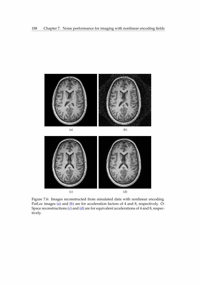
188 Chapter 7. Noise performance for imaging with nonlinear encoding fields
(a) (b)
(c) (d)
Figure 7.6: Images reconstructed from simulated data with nonlinear encoding.PatLoc images (a)(a) and (b)(b) are for acceleration factors of 4 and 8, respectively. O-Space reconstructions (c)(c) and (d)(d) are for equivalent accelerations of 4 and 8, respec-tively.

7.6. Discussion 189
fined by the Dirichlet kernel. PatLoc imposes a structure on the frame operator bythe careful selection of a nonuniformly spaced pixel basis. The structure allows foran exact performance analysis and a simple reconstruction algorithm, which aresignificant advantages of this scheme. The difficulty lies in displaying the nonuni-form pixels and often the pixel values are interpolated to a regular grid. This inter-polation reflects a loss in the fundamental resolution of the final pixels displayed.Regions with low variance may have large bias due to interpolation, which resultsin significant image blurring. On the other hand, O-space exhibits a relatively uni-form variance map, but suffers from a loss of resolution for increasing acceleration.Thus using variance as the sole metric will fail to capture the true imaging perfor-mance. In other words, the variance is necessary but not sufficient to quantify theperformance of nonlinear encoding schemes. A complete characterisation of theperformance of nonlinear encoding schemes must jointly examine the SNR andthe spatially-dependent resolution. It is foreseeable that a hybrid of variance andresolution metrics may prove the most useful for assessment. This is the directionof our current work.
The metric presented in this chapter does not capture the tradeoff betweenvariance and resolution, and will be of limited use for encoding schemes withlarge variation in resolution. These schemes require an appropriate pixel basis toimprove the conditioning of the reconstruction problem. This basis is naturallydefined for Cartesian PatLoc and is based on the Jacobian of the nonlinear map-ping associated with the encoding fields. For arbitrary schemes such as those inChapter 66, no such Jacobian can be defined. In this case, a direct reconstruction of auniform pixel basis will amplify noise in regions with minimal encoding, since theinherent pixel resolution is not compensated for. In reality, the reconstruction isregularised and the proposed metric no longer valid. However, for schemes suchas O-space, which have a relatively constant resolution, the metric is an effectivemeasure of the reconstruction variance.
The development of nonlinear imaging schemes has revealed the need to con-sider both the encoding fields and the coil sensitivities jointly in designing newstate-of-the-art imaging techniques. In additional to this encoding, spatial encod-ing can be provided by tailored RF excitation profiles which excite a different sub-set of spins every echo [122122]. In principle, the framework presented in this chapteris readily applicable to the performance analysis of schemes that utilise a combi-nation of nonlinear fields, multiple receive coils and tailored RF excitation.

190 Chapter 7. Noise performance for imaging with nonlinear encoding fields
7.7 Conclusion
In this chapter, we have developed a framework to analyse the noise performanceof imaging schemes with general nonlinear encoding fields. Each scheme is uniquelydefined by the spatial encoding functions which have a contribution from the accu-mulated phase function and the coil sensitivity. The encoding functions for a givenscheme define an associated frame operator, from which performance metrics arederived. Highly structured schemes such as SENSE and PatLoc exhibit a structurein the frame operator that can be exploited to provide the closed form performancemetrics reported in the literature. For arbitrary schemes such as O-space, the frameoperator can be used to define a tractable and intuitive noise metric based on thecovariance of the reconstructed pixels. We demonstrated the utility of this compu-tationally efficient performance metric through simulation examples.
The continued advancement of MRI relies on the ability to quantitatively assessnew techniques as they are created. The development of suitable performancemetrics, such as those presented in this chapter, will help guide designers to findoptimised imaging schemes that utilise all possible degrees of freedom.

7.A. Basis selection 191
Appendices
7.A Basis selection
The finite dimensional representation of the frame operator, described in Section 7.27.2,was developed using a pixel basis. We now turn our attention to the precise defi-nition of this basis. The basis should be capable of accurately representing the truefunction while allowing efficient computation of the encoding matrix in (7.167.16).Two common bases are the rectangular basis ζp(x) = 1
W rectW(x − xp) and theDirac delta basis χp(x) = δ(x− xp). The rectangular basis is more realistic whilethe delta basis is better for computation. In this section we calculate the differencebetween these two bases for simple linear encoding. We quantify the difference inthe reconstructed pixels between the delta basis and rectangular basis.
This investigation uses a one dimensional object with linear encoding to ex-amine the differences between the bases although the analysis can be extended tohigher dimensions and more complicated encoding schemes. The phase functionwe use for demonstration is
φi(x) = kix (7.93)
where ki is selected so the encoding functions, Φq,i, are the Fourier basis. Addi-tionally, an ideal volume coil is assumed such that cl(x) = 1. The measurementsare given by
yi =∫
m(x)e−jkixdx (7.94)
This equation is discretised with both χp and ζp. This is equivalent to makingone of the following approximations,
m(x) ≈ f (x) = ∑j
f jχj(x) = ∑j
f jδ(x− xj) (7.95)
m(x) ≈ g(x) = ∑j
gjζ j(x) = ∑j
gj1
W rectW
(x− xj) (7.96)
We denote the vector containing the coefficients of the delta basis approxima-tion as f = [ f1, . . . , fN ]
′. Likewise, the coefficient vector for the rectangular basisis g = [g1, . . . , gN ]
′ and the measurement vector is y = [y1, . . . , yNt ]′. Applying the
approximations above the measurement equation can be written as two different

192 Chapter 7. Noise performance for imaging with nonlinear encoding fields
matrix equations, depending on our choice of basis.
y = HE f (7.97)
y = GEg (7.98)
where Ei,n = e−jkixn is the Fourier matrix and the elements of the diagonalweighting matrices, H and G, are calculated by
αn =∫
χ(x)e−jknxdx (7.99)
which is the Fourier transform of the basis shape. This results in
H = diag(t1, . . . , tNt); ti = 1, i = 1, . . . , Nt (7.100)
G = diag(τ1, . . . , τNt); τi = sinc(Wki), i = 1, . . . , Nt (7.101)
We assume that both systems of equations can be inverted and note that E−1 =1n E′. Given the measurement vector, y, the reconstructed coefficients for both sys-tems are
f = E−1H−1y (7.102)
g = E−1G−1y (7.103)
These coefficients are displayed as image pixels in the reconstructed image;thus we are interested in the difference between both sets of coefficients. We cal-culate ‖ f − g‖ and use the fact that, ‖E−1y‖ = 1√
n‖y‖,
f − g = E−1(H−1 −G−1)y (7.104)
‖ f − g‖ = 1√n‖(H−1 −G−1)y‖ (7.105)
We consider y with elements defined by the continuous integral in (7.947.94) andassume that ki = (i − Nt/2)∆k where the frequency spacing, ∆k, is fixed (deter-mined from the reciprocal of the FOV). Furthermore, we assume that the Fouriertransform of m(x) has support in the interval [−Ω/2, Ω/2]. Denote K = Ω
∆kas the
number of non-zero measurements. Thus,
‖(H−1 −G−1)y‖22 = ‖ΥK(H−1 −G−1)y‖2
2 (7.106)
≤ ‖ΥK(H−1 −G−1)‖22 ‖y‖2
2 (7.107)
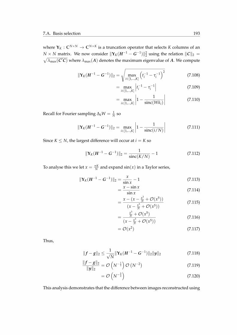
7.A. Basis selection 193
where ΥK : CN×N → CN×K is a truncation operator that selects K columns of anN × N matrix. We now consider ‖ΥK(H−1 − G−1)‖2
2 using the relation ‖C‖2 =√λmax(C′C) where λmax(A) denotes the maximum eigenvalue of A. We compute
‖ΥK(H−1 −G−1)‖2 =
√max
i∈[1,...,K]
(t−1i − τ−1
i
)2(7.108)
= maxi∈[1,...,K]
∣∣∣t−1i − τ−1
i
∣∣∣ (7.109)
= maxi∈[1,...,K]
∣∣∣∣1− 1sinc(Wki)
∣∣∣∣ (7.110)
Recall for Fourier sampling ∆kW = 1N so
‖ΥK(H−1 −G−1)‖2 = maxi∈[1,...,K]
∣∣∣∣1− 1sinc(i/N)
∣∣∣∣ (7.111)
Since K ≤ N, the largest difference will occur at i = K so
‖ΥK(H−1 −G−1)‖2 =1
sinc(K/N)− 1 (7.112)
To analyse this we let x = πKN and expand sin(x) in a Taylor series,
‖ΥK(H−1 −G−1)‖2 =x
sin x− 1 (7.113)
=x− sin x
sin x(7.114)
=x− (x− x3
3! +O(x5))
(x− x3
3! +O(x5))(7.115)
=x3
3! +O(x5)
(x− x3
3! +O(x5))(7.116)
= O(x2) (7.117)
Thus,
‖ f − g‖2 ≤1√N‖ΥK(H−1 −G−1)‖2‖y‖2 (7.118)
‖ f − g‖2
‖y‖2= O
(N−
12
)O(
N−2) (7.119)
= O(
N−52
)(7.120)
This analysis demonstrates that the difference between images reconstructed using

194 Chapter 7. Noise performance for imaging with nonlinear encoding fields
a delta basis and rectangular basis decays rapidly for increasing N. In other words,the difference between the delta basis and rectangular basis is negligible for a finelyspaced pixel grid. Although this is well accepted in the research community, arigourous analysis such as above has to the best of our knowledge, not appearedin the literature.

CHAPTER 8
Conclusion
THE fundamental aim of MRI is to non-invasively determine the detailed struc-ture and function of a human body. This information is used for the diagnosis
and treatment of patients as well as fundamental neuroscience and pathology. Tosatisfy all these applications, ideally MRI would be able to classify tissue, detectand localise diseases, and map different functions of the brain.
This ambitious goal is challenging for a multitude of reasons. The structure ofthe body is made up of an enormous number of atoms. MRI is only sensitive toatoms with a particular spin. Further, these spins are not directly observable; mea-surements only represent the average behaviour of the relevant spins. To makematters worse, the number of measurements is severely limited due to physicalconstraints, hardware constraints and safety constraints. Reasonably, one can ex-pect that limited information will be attainable from the measurements of such asystem.
The saving grace of MRI is also its main limitation – the ability to improveone property of the system at the expense of another. These tradeoffs are eitherinherent in the physical principles or imposed by the engineer.
The overarching conclusion of this thesis is the following. In order to maximisethe performance of MRI for a specific application, one must jointly consider accurate signalmodels, algorithm design and acquisition strategies.
Although this statement is intuitive, the results in this thesis highlight severalareas where performance improvements can be made by following this principle.
8.1 Summary of original contributions
Chapter 44 examined the tradeoff in Fourier reconstruction between SNR (relatedto sampling bandwidth) and image distortion. In the context of the estimation oftransverse relaxation times, this translates to a tradeoff between bias and variance.A detailed analysis of the estimation problem revealed that the bias is often sub-stantial when a simplified signal model is assumed. To overcome this, the estima-tion problem was reposed using an accurate signal model, which incorporates theimage distortion. A Bayesian algorithm was developed using the improved signal
195

196 Chapter 8. Conclusion
model to overcome the bias/variance tradeoff. Improved results were demon-strated at the expense of increased algorithm complexity and computation time.
Chapter 55 analysed the problem of estimating a distribution of relaxation times,which is more representative of the underlying structure than the assumption of aunique discrete component. However, it was shown that the accurate estimationof some properties of this distribution is infeasible due to the spin averaging. Itwas concluded from the results that although the location of the distribution com-ponents can be accurately estimated, the distribution width cannot be determinedfrom typical measurements. Current state-of-the art techniques employ regularisa-tion to improve the estimation results although this can unfavourably bias the dis-tribution shape. This highlights the important point that one should not attemptto extract more information than is available in the measurements. The alternativeproposed in this thesis is to estimate the locations of the distribution mass, assum-ing a width of zero. This assumption is justified since the width has minimal effecton the measurements; indeed this is the same reason the width cannot be esti-mated. The resulting estimation problem was cast in a Bayesian framework, fromwhich a computationally efficient and reliable algorithm was developed. The algo-rithm exhibits near-optimal performance and improves on the currently availabletechniques.
Chapter 66 delved into the emerging field of nonlinear spatial encoding. Aunique property of these techniques is that, unlike linear encoding, the fundamen-tal resolution is spatially varying. This create both challenges and opportunities.A novel acquisition strategy was developed to improve the image resolution in auser-specified region. The technique uses nonlinear encoding fields together withthe design of optimal gradient waveforms. In this way the spatially varying res-olution inherent in nonlinear fields is exploited to improve the spatial encodingin the region of interest. The result is an image with enhanced resolution in thedesired region at the expense of pronounced blurring in other regions. This directtradeoff is useful for applications that are only interested in a particular region.This is often the case for brain imaging as practitioners may be focused on the re-gion surrounding a brain tumour, or on the function of sub-cortical structures suchas the hippocampus. Another application is cardiac imaging where the acquisitioncould be designed to optimally encode the heart region.
Chapter 77 revisited the basic image reconstruction problem applicable for en-coding with nonlinear fields. The image reconstruction problem was recast usingframe theory to provide a novel perspective on the noise properties of existingtechniques. The source of aliasing and noise amplification for these techniqueswas elucidated using the Dirichlet kernel. Additionally, a computationally effi-

8.2. Future work 197
cient and intuitive noise metric was developed, based on an approximation of thereconstructed pixel covariance. This novel metric is applicable to general encodingschemes that use any combination of linear and nonlinear fields.
The work in this thesis underscores the importance of rigourously analysingthe signals obtained from MRI experiments. The accuracy of estimated biologicalparameters was examined in Chapters 44 and 55. In both chapters, an initial analysislead to an improved signal model and estimation algorithm. The spatially varyingresolution inherent in nonlinear encoding fields was investigated in Chapter 66,which lead to novel acquisition strategies. Finally, the noise variance associatedwith image reconstruction of general encoding schemes was explored in Chapter 77,which we anticipate will be useful to evaluate emerging new techniques.
8.2 Future work
Although impressive performance is achievable with modern MRI technology,there are many opportunities for further enhancements. This thesis has demon-strated several specific improvements that can be made to current state-of-the-arttechniques. Additionally, this work has confirmed that detailed signal analysis canlead to new insights and the development of novel techniques. This paradigm canalso serve as a roadmap for future development.
8.2.1 Statistical estimation
The statistical estimation algorithms developed in this thesis are most useful forsituations with low SNR. In this case, improved signal models and computation-ally demanding algorithms are required to extract the maximum amount of in-formation available from the noisy measurements. Future research could applysimilar algorithms to the recent applications of portable MRI and ultra-low fieldimaging, since these operate at inherently low SNR. The increased computationand complexity is mitigated by the dramatic increasing in computing performancein recent years. This, coupled with a reduction in hardware cost, makes the appli-cation of advanced estimation algorithms feasible.
Further research can be conducted into the estimation algorithms developedin this thesis. Improvements to the computational performance of the Gibbs sam-pling algorithm of Chapter 44 is required to make this technique feasible in a clinicalsetting. For example, the spatial variation of T2 could be modelled with a Markovrandom field to capture the local similarities of biological tissue. This prior in-formation would improve the sampling performance of the estimation algorithm.

198 Chapter 8. Conclusion
The progressive correction technique in Chapter 55 would benefit from a theoreticalanalysis and proof that the posterior density approximation approaches the opti-mal density. In principle, diffusion weighting could also be added to the CPMGsequence and incorporated into the signal model, in order to distinguish the ex-change component of the T2 model.
8.2.2 Nonlinear encoding
Nonlinear spatial encoding is still a relatively new idea and future research cantake a number of directions. Generalised encoding with multiple gradient chan-nels incorporating linear and nonlinear fields adds degrees of freedom to the de-sign of acquisition strategies. How to best utilise the extra degrees of freedom fora given application remains an open question. The optimisation in Chapter 66 isbased on the single criteria of local k-space trajectories. Other factors such as noiseperformance, receive coil geometries, and acquisition speed may be incorporatedinto gradient waveform design.
A detailed investigation into peripheral nerve stimulation is required to verifythe hypothesis that nonlinear encoding can reduce the risk of nerve stimulation.Although it is challenging to incorporate all factors that lead to peripheral nervestimulation, such a study will be necessary prior to the clinical adoption of nonlin-ear encoding.
Chapter 77 analyses the SNR of general nonlinear encoding schemes. The per-formance metric developed, although useful, is not perfect. The covariance ap-proximation relies on a diagonally dominant frame matrix, which neglects thestructure of the off-diagonal terms. An ideal noise analysis would consider all thenuances of the encoding scheme, without having to compute the entire covariancematrix.
In addition to noise performance, further research is required into the resolu-tion of nonlinear encoding schemes. Currently, resolution metrics are based onthe point spread function which depends on the reconstruction choice. A met-ric that depends only on the encoding scheme would be useful to determine thefundamental resolvability of neighbouring features in the presence of noise. Anal-ogous to the Cramér-Rao lower bound, an ideal resolution metric would providea benchmark for reconstruction algorithms, not depend on them.
A complete characterisation of the imaging performance of nonlinear encod-ing schemes requires a joint analysis of both noise and resolution. A metric thatcombines both quantities would prove useful. The mean squared error naturallycombines the quantities of bias and variance into a single performance metric and
8.2. Future work 199
is often used to benchmark different techniques. The prevalence of this error met-ric suggests that researchers working on nonlinear encoding could benefit from ananalogous metric that combines SNR and resolution.
8.2.3 Signal modelling
There are signal dependencies other than those addressed in this thesis that areoften not modelled. These include magnetic susceptibility, diffusion, blood flowand partial volume effects to name just a few. Simple assumptions about theseprocesses causes a mismatch between the assumed signal model and the actualmeasurements. This is often referred to as ‘systematic error’ in MRI literature or‘model uncertainty’ in signal processing literature. The mismatch is problematicfor image reconstruction and leads to non-convergent algorithms or ill-definedartifacts. This problem could be alleviated by incorporating these effects into theappropriate signal model and reconstruction algorithm.
Further research is needed to quantify the effect of model uncertainty on im-age reconstruction and parameter estimation. As the boundaries of performanceare pushed and more information is extracted from noisy measurements, clini-cians will need measures of certainty in order to completely trust the images andparameter maps that are produce from an MRI scanner.


Bibliography
[1] M. Poole, Improved equipment and techniques for dynamic shimming in high field MRI.PhD thesis, The University of Nottingham, 2007. (Cited on page 11.)
[2] A. Macovski and S. Conolly, “Novel approaches to low-cost MRI,” Magnetic Reso-nance in Medicine, vol. 30, no. 2, pp. 221–230, 1993. (Cited on pages 22 and 7676.)
[3] J. P. Mugler and J. R. Brookeman, “The optimum data sampling period for maximumsignal-to-noise ratio in MR imaging,” Reviews of magnetic resonance in medicine, vol. 3,no. 1, pp. 1–51, 1988. (Cited on pages 33 and 6060.)
[4] E. M. Haacke, “The effects of finite sampling in spin-echo or field-echo magneticresonance imaging,” Magnetic Resonance in Medicine, vol. 4, no. 5, pp. 407–421, 1987.(Cited on pages 33 and 6060.)
[5] K. P. Whittall and A. L. MacKay, “Quantitative interpretation of NMR relaxationdata,” Journal of Magnetic Resonance (1969), vol. 84, no. 1, pp. 134–152, 1989. (Citedon pages 44, 8686, 9090 and 9191.)
[6] S. M. Kay, Fundamentals of statistical signal processing: Estimation theory. Prentice-Hall,1993. (Cited on pages 44, 9292, 9393, 9494 and 167167.)
[7] J. L. Lancaster, T. Andrews, L. J. Hardies, S. Dodd, and P. T. Fox, “Three-pool modelof white matter,” Journal of Magnetic Resonance Imaging, vol. 17, no. 1, pp. 1–10, 2003.(Cited on pages 44, 8686, 9191 and 9494.)
[8] T. Andrews, J. L. Lancaster, S. J. Dodd, C. Contreras-Sesvold, and P. T. Fox, “Testingthe three-pool white matter model adapted for use with T2 relaxometry,” MagneticResonance in Medicine, vol. 54, no. 2, pp. 449–454, 2005. (Cited on pages 44, 8686, 8787, 9292and 9494.)
[9] J. Hennig, A. Welz, G. Schultz, J. Korvink, Z. Liu, O. Speck, and M. Zaitsev, “Parallelimaging in non-bijective, curvilinear magnetic field gradients: A concept study,”Magnetic Resonance Materials in Physics, Biology and Medicine, vol. 21, pp. 5–14, 2008.(Cited on pages 44, 126126 and 130130.)
[10] G. Schultz, P. Ullmann, H. Lehr, A. Welz, J. Hennig, and M. Zaitsev, “Reconstruc-tion of MRI data encoded with arbitrarily shaped, curvilinear, nonbijective magneticfields,” Magnetic Resonance in Medicine, vol. 64, no. 5, pp. 1390–1403, 2010. (Cited onpages 44, 126126, 129129, 130130, 155155, 160160, 168168, 172172, 173173, 181181, 183183 and 184184.)
[11] J. P. Stockmann, P. A. Ciris, G. Galiana, L. Tam, and R. T. Constable, “O-space imag-ing: Highly efficient parallel imaging using second-order nonlinear fields as encod-ing gradients with no phase encoding,” Magnetic Resonance in Medicine, vol. 64, no. 2,pp. 447–456, 2010. (Cited on pages 44, 126126, 130130, 140140, 180180, 183183, 184184 and 187187.)
201

202 Bibliography
[12] D. Gallichan, C. A. Cocosco, A. Dewdney, G. Schultz, A. Welz, J. Hennig, and M. Za-itsev, “Simultaneously driven linear and nonlinear spatial encoding fields in MRI,”Magnetic Resonance in Medicine, vol. 65, no. 3, pp. 702–714, 2011. (Cited on pages 44,126126, 129129, 130130, 134134, 143143, 155155, 160160 and 181181.)
[13] O. Christensen, Frames and bases: An introductory course. Birkhäuser, 2008. (Cited onpages 44, 160160 and 162162.)
[14] K. Pruessmann, M. Weiger, M. Scheidegger, and P. Boesiger, “SENSE: sensitivityencoding for fast MRI,” Magnetic Resonance in Medicine, vol. 42, no. 5, pp. 952–962,1999. (Cited on pages 44, 133133, 136136, 160160, 165165, 167167, 168168, 169169 and 173173.)
[15] M. H. Levitt, Spin dynamics: basics of nuclear magnetic resonance. John Wiley and Sons,2001. (Cited on pages 99, 2424 and 3131.)
[16] F. Bloch, “Nuclear induction,” Physics Review, vol. 70, pp. 460–473, 1946. (Cited onpage 99.)
[17] K. Blum, Density matrix theory and applications. Plenum Press, second ed., 1996. (Citedon pages 1111 and 1616.)
[18] E. Merzbacher, Quantum mechanics. John Wiley and Sons, third ed., 2004. (Cited onpage 1212.)
[19] I. I. Rabi, N. F. Ramsey, and J. Schwinger, “Use of rotating coordinates in magneticresonance problems,” Rev. Mod. Phys., vol. 26, pp. 167–171, Apr 1954. (Cited onpage 1212.)
[20] J. Cavanagh, W. J. Fairbrother, A. G. Palmer, III, and N. J. Skelton, Protein NMRspectroscopy, principles and practice. Academic Press, 1996. (Cited on pages 2020 and 2727.)
[21] J. T. Bushberg, J. A. Seibert, E. M. Leidholdt, and J. M. Boone, The essential physicsof medical imaging. Lippincott Williams and Wilkins, second ed., 2002. (Cited onpages 2121 and 2222.)
[22] P. A. Bottomley, T. H. Foster, R. E. Argersinger, and L. M. Pfeifer, “A review of nor-mal tissue hydrogen NMR relaxation times and relaxation mechanisms from 1–100MHz: dependence on tissue type, NMR frequency, temperature, species, excision,and age,” Medical Physics, vol. 11, pp. 425–448, 1984. (Cited on page 2121.)
[23] A. Abragam, The principles of nuclear magnetism. London: Oxford University Press,1961. (Cited on pages 2525 and 2626.)
[24] P. Luginbühl and K. Wüthrich, “Semi-classical nuclear spin relaxation theory revis-ited for use with biological macromolecules,” Progress in Nuclear Magnetic ResonanceSpectroscopy, vol. 40, no. 3, pp. 199–247, 2002. (Cited on page 2727.)
[25] A. G. Redfield, “On the theory of relaxation processes,” IBM J. Res. Dev, vol. 1,pp. 19–31, 1957. (Cited on page 2828.)

Bibliography 203
[26] M. Alecci, C. M. Collins, M. B. Smith, and P. Jezzard, “Radio frequency magneticfield mapping of a 3 Tesla birdcage coil: Experimental and theoretical dependenceon sample properties,” Magnetic Resonance in Medicine, vol. 46, no. 2, pp. 379–385,2001. (Cited on page 3737.)
[27] E. L. Hahn, “Spin echoes,” Physical Review, vol. 80, pp. 580–594, 1950. (Cited onpage 3838.)
[28] H. Y. Carr and E. M. Purcell, “Effects of diffusion on free precession in nuclear mag-netic resonance experiments,” Phys. Rev., vol. 94, pp. 630–638, May 1954. (Cited onpages 3838 and 6060.)
[29] S. Meiboom and D. Gill, “Modified spin-echo method for measuring nuclear relax-ation times,” Review of Scientific Instruments, vol. 29, no. 8, pp. 688–691, 1958. (Citedon pages 3838 and 6060.)
[30] S. Ljunggren, “A simple graphical representation of Fourier-based imaging meth-ods,” Journal of Magnetic Resonance, vol. 54, pp. 338–343, 1983. (Cited on page 4444.)
[31] D. B. Twieg, “The k-trajectory formulation of the NMR imaging process with appli-cations in analysis and synthesis of imaging methods,” Medical Physics, vol. 10, no. 5,pp. 610–621, 1983. Times Cited: 154. (Cited on page 4444.)
[32] M. L. Lauzon and B. K. Rutt, “Effects of polar sampling in k-space,” Magnetic Reso-nance in Medicine, vol. 36, no. 6, pp. 940–949, 1996. (Cited on pages 4545 and 4747.)
[33] P. Lauterbur, “Image formation by induced local interactions: examples employingnuclear magnetic resonance,” Nature, vol. 242, no. 5394, pp. 190–191, 1973. (Cited onpage 4747.)
[34] M. O’Donnell and W. A. Edelstein, “NMR imaging in the presence of magnetic fieldinhomogeneities and gradient field nonlinearities,” Medical Physics, vol. 12, pp. 20–26, 1985. (Cited on page 4747.)
[35] J. R. Reichenbach, R. Venkatesan, D. A. Yablonskiy, M. R. Thompson, S. Lai, andE. M. Haacke, “Theory and application of static field inhomogeneity effects ingradient-echo imaging,” Journal of Magnetic Resonance Imaging, vol. 7, no. 2, pp. 266–279, 1997. (Cited on page 4747.)
[36] K. Scheffler and J. Hennig, “Reduced circular field-of-view imaging,” Magnetic Res-onance in Medicine, vol. 40, no. 3, pp. 474–480, 1998. (Cited on page 4949.)
[37] P. Mansfield, A. A. Maudsley, and T. Bains, “Fast scan proton density imaging byNMR,” Journal of Physics E: Scientific Instruments, vol. 9, no. 4, pp. 271–278, 1976.(Cited on page 4949.)
[38] I. L. Pykett and R. R. Rzedzian, “Instant images of the body by magnetic resonance,”Magnetic Resonance in Medicine, vol. 5, no. 6, pp. 563–571, 1987. (Cited on page 4949.)

204 Bibliography
[39] M. S. Cohen and R. M. Weisskoff, “Ultra-fast imaging,” Magnetic Resonance Imaging,vol. 9, no. 1, pp. 1–37, 1991. (Cited on page 4949.)
[40] C. P. Davis, G. C. Mckinnon, J. F. Debatin, and G. K. Schulthess, “Ultra-high-speedMR imaging,” European Radiology, vol. 6, pp. 297–311, 1996. (Cited on pages 4949and 155155.)
[41] J. A. Den Boer, J. D. Bourland, J. A. Nyenhuis, C. L. Ham, J. M. Engels, F. X. Hebrank,G. Frese, and D. J. Schaefer, “Comparison of the threshold for peripheral nerve stim-ulation during gradient switching in whole body MR systems,” Journal of MagneticResonance Imaging, vol. 15, no. 5, pp. 520–525, 2002. (Cited on page 5050.)
[42] P. P. M. So, M. A. Stuchly, and J. A. Nyenhuis, “Peripheral nerve stimulation bygradient switching fields in magnetic resonance imaging,” Biomedical Engineering,IEEE Transactions on, vol. 51, no. 11, pp. 1907–1914, 2004. (Cited on pages 5050 and 156156.)
[43] H. Zeng and R. T. Constable, “Image distortion correction in EPI: Comparison offield mapping with point spread function mapping,” Magnetic Resonance in Medicine,vol. 48, no. 1, pp. 137–146, 2002. (Cited on page 5050.)
[44] Z. P. Liang and P. C. Lauterbur, Principles of magnetic resonance imaging: a signal pro-cessing perspective. IEEE Press, 2000. (Cited on page 5151.)
[45] S. Kaczmarz, “Angenäherte auflösung von systemen linearer gleichungen,” Bull. Int.Acad. Polon. Sci. A, vol. 35, pp. 355–357, 1937. (Cited on pages 5252 and 184184.)
[46] R. Gordon, R. Bender, and G. T. Herman, “Algebraic Reconstruction Techniques(ART) for three-dimensional electron microscopy and X-ray photography,” Journalof Theoretical Biology, vol. 29, no. 3, pp. 471–481, 1970. (Cited on page 5252.)
[47] G. T. Herman, Fundamentals of computerized tomography: Image reconstruction from pro-jections. Springer, second ed., 2009. (Cited on page 5252.)
[48] M. Hestenes and E. Stiefel, “Methods of conjugate gradients for solving linear sys-tems,” Journal of Research of the National Bureau of Standards, vol. 49, no. 6, pp. 409–436,1952. (Cited on page 5252.)
[49] K. Pruessmann, M. Weiger, P. Börnert, and P. Boesiger, “Advances in sensitivity en-coding with arbitrary k-space trajectories,” Magnetic Resonance in Medicine, vol. 46,no. 4, pp. 638–651, 2001. (Cited on page 5252.)
[50] Luenberger, Introduction to linear and nonlinear programming. Kluwer Academic Pub-lishers, second ed., 2003. (Cited on page 5353.)
[51] J. Johnson, “Thermal agitation of electricity in conductors,” Physical Review, vol. 32,no. 1, pp. 97–109, 1928. (Cited on page 5353.)
[52] H. Nyquist, “Thermal agitation of electric charge in conductors,” Physical Review,vol. 32, no. 1, pp. 110–113, 1928. (Cited on page 5353.)

Bibliography 205
[53] E. M. Haacke, R. W. Brown, M. R. Thompson, and R. Venkatesan, Magnetic resonanceimaging: Physical principles and sequence design. John Wiley and Sons, 1999. (Cited onpages 5454, 6969 and 7777.)
[54] W. A. Edelstein, G. H. Glover, C. J. Hardy, and R. W. Redington, “The intrinsicsignal-to-noise ratio in NMR imaging,” Magnetic Resonance in Medicine, vol. 3, no. 4,pp. 604–618, 1986. (Cited on page 5454.)
[55] C. R. Haider, H. H. Hu, N. G. Campeau, J. Huston, and S. J. Riederer, “3D hightemporal and spatial resolution contrast-enhanced MR angiography of the wholebrain,” Magnetic Resonance in Medicine, vol. 60, no. 3, pp. 749–760, 2008. (Cited onpage 5555.)
[56] J. Tsao, P. Boesiger, and K. P. Pruessmann, “k-t BLAST and k-t SENSE: Dynamic MRIwith high frame rate exploiting spatiotemporal correlations,” Magnetic Resonance inMedicine, vol. 50, no. 5, pp. 1031–1042, 2003. (Cited on page 5555.)
[57] I. R. Levesque and G. B. Pike, “Characterizing healthy and diseased white matterusing quantitative magnetization transfer and multicomponent T2 relaxometry: Aunified view via a four-pool model,” Magnetic Resonance in Medicine, vol. 62, no. 6,pp. 1487–1496, 2009. (Cited on page 6060.)
[58] A. L. MacKay, I. M. Vavasour, A. Rauscher, S. H. Kolind, B. MÃd’dler, G. R. W.Moore, A. L. Traboulsee, D. K. B. Li, and C. Laule, “MR relaxation in multiple scle-rosis,” Neuroimaging Clinics of North America, vol. 19, no. 1, pp. 1–26, 2009. (Cited onpage 6060.)
[59] G. Bartzokis, T. Tishler, P. Lu, P. Villablanca, L. Altshuler, M. Carter, D. Huang, N. Ed-wards, and J. Mintz, “Brain ferritin iron may influence age- and gender-related risksof neurodegeneration,” Neurobiology of Aging, vol. 28, no. 3, pp. 414–423, 2007. (Citedon page 6060.)
[60] L. A. Shepp and B. F. Logan, “The fourier reconstruction of a head section,” NuclearScience, IEEE Transactions on, vol. 21, no. 3, pp. 21–43, 1974. (Cited on page 6464.)
[61] S. Geman and D. Geman, “Stochastic relaxation, Gibbs distributions, and thebayesian restoration of images,” IEEE Transactions on Pattern Analysis and MachineIntelligence, vol. PAMI-6, no. 6, pp. 721–741, 1984. (Cited on page 7272.)
[62] A. Smith and G. Roberts, “Bayesian computation via the Gibbs sampler and relatedMarkov chain Monte Carlo methods,” Journal of the Royal Statistical Society. Series B(Methodological), vol. 55, no. 1, pp. 3–23, 1993. (Cited on page 7272.)
[63] C. Ritter and M. Tanner, “Facilitating the Gibbs sampler: the Gibbs stopper and thegriddy-Gibbs sampler,” J. Amer. Statistical Assoc., vol. 87, no. 419, pp. 861–868, 1992.(Cited on page 7272.)

206 Bibliography
[64] J. S. Lui, Monte Carlo Strategies in Scientific Computing. Springer, 2008. (Cited onpage 7373.)
[65] K. Uludag, B. Müller-Bierl, and K. Ugurbil, “An integrative model for neuronalactivity-induced signal changes for gradient and spin echo functional imaging,”NeuroImage, vol. 48, pp. 150–165, 2009. (Cited on page 7474.)
[66] D. Price, I. Delakis, C. Renaud, and R. Dickinson, “MRI scanners: a buyer’s guide.”(Cited on page 7676.)
[67] P. Bloomfield, Fourier analysis of time series: an introduction. John Wiley & Sons, 2000.(Cited on page 7878.)
[68] M. Abramowitz and I. A. Stegun, Handbook of mathematical functions with formulas,graphs, and mathematical tables. Dover, 1964. (Cited on page 7979.)
[69] A. MacKay, C. Laule, I. Vavasour, T. Bjarnason, S. Kolind, and B. Mädler, “Insightsinto brain microstructure from the T2 distributions,” Magnetic Resonance Imaging,vol. 24, no. 4, pp. 515–525, 2006. (Cited on page 8686.)
[70] C. Poon and R. Henkelman, “Practical T2 quantitation for clinical applications,”Journal of Magnetic Resonance Imaging, vol. 2, no. 5, pp. 541–553, 1992. (Cited onpage 8686.)
[71] J. Hennig, “Multiecho imaging sequences with low refocusing flip angles,” J MagnReson, vol. 78, no. 3, pp. 397–407, 1988. (Cited on pages 8686 and 8989.)
[72] J. Hennig, “Echoes–how to generate, recognize, use or avoid them in MR-imagingsequences. Part I: Fundamental and not so fundamental properties of spin echoes,”Concepts in Magnetic Resonance, vol. 3, no. 3, pp. 125–143, 1991. (Cited on pages 8686,8989 and 117117.)
[73] G. J. Stanisz, E. E. Odrobina, J. Pun, M. Escaravage, S. J. Graham, M. J. Bronskill, andR. M. Henkelman, “T1, T2 relaxation and magnetization transfer in tissue at 3T,”Magnetic Resonance in Medicine, vol. 54, no. 3, pp. 507–512, 2005. (Cited on pages 8686and 9090.)
[74] A. Mackay, K. Whittall, J. Adler, D. Li, D. Paty, and D. Graeb, “In vivo visualizationof myelin water in brain by magnetic resonance,” Magnetic Resonance in Medicine,vol. 31, no. 6, pp. 673–677, 1994. (Cited on pages 8686 and 9090.)
[75] K. Whittall, A. Mackay, D. Graeb, R. Nugent, D. Li, and D. Paty, “In vivo mea-surement of T2 distributions and water contents in normal human brain,” MagneticResonance in Medicine, vol. 37, no. 1, pp. 34–43, 1997. (Cited on pages 8686, 9090, 103103, 107107and 115115.)
[76] S. Zheng and Y. Xia, “On the measurement of multi-component T2 relaxation incartilage by MR spectroscopy and imaging,” Magnetic Resonance Imaging, vol. 28,no. 4, pp. 537–545, 2010. (Cited on pages 8686 and 9090.)

Bibliography 207
[77] T. Prasloski, B. Mädler, Q.-S. Xiang, A. MacKay, and C. Jones, “Applications ofstimulated echo correction to multicomponent T2 analysis,” Magnetic Resonance inMedicine, 2011. (in press). (Cited on pages 8686, 9090, 9191, 9494, 103103, 107107 and 115115.)
[78] K. J. Layton, M. Morelande, P. M. Farrell, B. Moran, and L. A. Johnston, “An im-proved algorithm for the estimation of multi-component T2 distributions,” in Pro-ceedings of the ISMRM 20th Scientific Meeting and Exhibition, (Melbourne), p. 2395,2012. (Cited on page 8686.)
[79] R. M. Lebel and A. H. Wilman, “Transverse relaxometry with stimulated echo com-pensation,” Magnetic Resonance in Medicine, vol. 64, no. 4, pp. 1005–1014, 2010. (Citedon pages 8787, 9090, 9191, 9292, 9494, 103103, 107107 and 116116.)
[80] K. J. Layton, L. A. Johnston, P. M. Farrell, B. Moran, and M. Morelande, “Estimationof relaxation time distributions in magnetic resonance imaging,” in Proceedings of theIEEE Conference on Acoustics, Speech, and Signal Processing, pp. 697–700, 2012. (Citedon page 8787.)
[81] J. Sijbers and A. J. Den Dekker, “Maximum likelihood estimation of signal amplitudeand noise variance from MR data,” Magnetic Resonance in Medicine, vol. 51, no. 3,pp. 586–594, 2004. (Cited on pages 9090 and 9999.)
[82] S. J. Graham, P. L. Stanchev, and M. J. Bronskill, “Criteria for analysis of multicom-ponent tissue T2 relaxation data,” Magnetic Resonance in Medicine, vol. 35, no. 3,pp. 370–378, 1996. (Cited on page 9191.)
[83] N. Oudjane and C. Musso, “Progressive correction for regularized particle filters,” inProceedings of the Third International Conference on Information Fusion, vol. 2, pp. 10–17,2002. (Cited on page 9999.)
[84] S. Kirkpatrick, C. D. Gelatt, and M. P. Vecchi, “Optimization by simulated anneal-ing,” Science, vol. 220, no. 4598, pp. 671–680, 1983. (Cited on page 100100.)
[85] J. Wang, M. Qiu, Q. X. Yang, M. B. Smith, and R. T. Constable, “Measurement andcorrection of transmitter and receiver induced nonuniformities in vivo,” MagneticResonance in Medicine, vol. 53, no. 2, pp. 408–417, 2005. (Cited on page 105105.)
[86] H. Akaike, “A new look at the statistical model identification,” IEEE Transactions onAutomatic Control, vol. 19, no. 6, pp. 716–723, 1974. (Cited on page 111111.)
[87] K. P. Burnham and D. R. Anderson, Model selection and multimodel inference: a practicalinformation-theoretic approach. Springer, 2nd ed., 2002. (Cited on pages 111111 and 115115.)
[88] G. Schwarz, “Estimating the dimension of a model,” The Annals of Statistics, vol. 6,no. 2, pp. 461–464, 1978. (Cited on page 111111.)
[89] M. T. Chao, “The asymptotic behavior of Bayes’ estimators,” The Annals of Mathe-matical Statistics, vol. 41, no. 2, pp. 601–608, 1970. (Cited on page 111111.)

208 Bibliography
[90] H. Iwaoka, T. Hirata, and H. Matsuura, “Optimal pulse sequences for magnetic reso-nance imaging-computing accurate T1, T2, and proton density images,” IEEE Trans-actions on Medical Imaging, vol. 6, pp. 360–369, dec. 1987. (Cited on page 112112.)
[91] L. Tam, J. P. Stockmann, and R. T. Constable, “Null space imaging: a novel gradientencoding strategy for highly efficient parallel imaging,” in Proceedings of the ISMRM18th Annual Meeting, (Stockholm), p. 2868, 2010. (Cited on pages 126126 and 181181.)
[92] D. Noll, “Rapid MR image acquisition in the presence of background gradients,” inBiomedical Imaging, 2002. Proceedings. 2002 IEEE International Symposium on, pp. 725–728, 2002. (Cited on page 129129.)
[93] B. A. Hargreaves, D. G. Nishimura, and S. M. Conolly, “Time-optimal multidimen-sional gradient waveform design for rapid imaging,” Magnetic Resonance in Medicine,vol. 51, no. 1, pp. 81–92, 2004. (Cited on page 135135.)
[94] M. Griswold, P. Jakob, R. Heidemann, M. Nittka, V. Jellus, J. Wang, B. Kiefer, andA. Haase, “Generalized autocalibrating partially parallel acquisitions (GRAPPA),”Magnetic Resonance in Medicine, vol. 47, no. 6, pp. 1202–1210, 2002. (Cited onpages 136136 and 160160.)
[95] S. Boyd and L. Vandenberghe, Convex Optimization. Cambridge University Press,2009. (Cited on page 139139.)
[96] G. Schultz, A. Welz, J. Hennig, and M. Zaitsev, “Generalized two-dimensional or-thogonal spatial encoding fields,” in Proceedings of the ISMRM 16th Annual Meeting,p. 2992, 2008. (Cited on page 139139.)
[97] A. M. Welz, M. Zaitsev, F. Jia, Z. Liu, J. Korvink, H. Schmidt, H. Lehr, H. Post,A. Dewney, and J. Hennig, “Development of a non-shielded PatLoc gradient insertfor human head imaging,” in Proceedings of the ISMRM 17th Scientific Meeting andExhibition, p. 3073, 2009. (Cited on page 143143.)
[98] O. Speck, J. Stadler, and M. Zaitsev, “High resolution single-shot EPI at 7T,” MagneticResonance Materials in Physics, Biology and Medicine, vol. 21, pp. 73–86, 2008. (Citedon page 144144.)
[99] J. H. Duyn, Y. Yang, J. A. Frank, and J. W. van der Veen, “Simple correction methodfor k-space trajectory deviations in MRI,” Journal of Magnetic Resonance, vol. 132,no. 1, pp. 150–153, 1998. (Cited on page 144144.)
[100] D. Norris and J. Hutchison, “Concomitant magnetic field gradients and their ef-fects on imaging at low magnetic field strengths,” Magnetic Resonance Imaging, vol. 8,no. 1, pp. 33–37, 1990. (Cited on page 144144.)
[101] P. Jezzard, A. S. Barnett, and C. Pierpaoli, “Characterization of and correction foreddy current artifacts in echo planar diffusion imaging,” Magnetic Resonance inMedicine, vol. 39, no. 5, pp. 801–812, 1998. (Cited on page 144144.)

Bibliography 209
[102] K. F. King, A. Ganin, X. J. Zhou, and M. A. Bernstein, “Concomitant gradient fieldeffects in spiral scans,” Magnetic Resonance in Medicine, vol. 41, no. 1, pp. 103–112,1999. (Cited on page 144144.)
[103] N. D. Zanche, C. Barmet, J. A. Nordmeyer-Massner, and K. P. Pruessmann, “NMRprobes for measuring magnetic fields and field dynamics in MR systems,” MagnReson Med, vol. 60, pp. 176–186, Jul 2008. (Cited on page 144144.)
[104] P. Sipilä, D. Lange, S. Lechner, W. Löw, P. Gross, M. Baller, G. Wachutka, andF. Wiesinger, “Robust, susceptibility-matched NMR probes for compensation ofmagnetic field imperfections in magnetic resonance imaging (MRI),” Sensors and Ac-tuators A: Physical, vol. 145–146, pp. 139–146, 2008. (Cited on page 144144.)
[105] C. Barmet, B. J. Wilm, M. Pavan, and K. P. Pruessmann, “A third-order field camerawith microsecond resolution for MR system diagnostics,” in Proceedings ISMRM,17th Scientific Meeting and Exhibition, (Honolulu), p. 781, 2009. (Cited on pages 144144and 145145.)
[106] C. Barmet, N. D. Zanche, and K. P. Pruessmann, “Spatiotemporal magnetic fieldmonitoring for MR,” Magnetic Resonance in Medicine, vol. 60, no. 1, pp. 187–197, 2008.(Cited on pages 144144 and 145145.)
[107] H. Han, R. P. MacGregor, and B. J. Balcom, “Pure phase encode magnetic field gra-dient monitor,” Journal of Magnetic Resonance, vol. 201, pp. 212–217, Dec 2009. (Citedon page 144144.)
[108] B. J. Wilm, C. Barmet, M. Pavan, and K. P. Pruessmann, “Higher order reconstructionfor MRI in the presence of spatiotemporal field perturbations,” Magnetic Resonancein Medicine, vol. 65, no. 6, pp. 1690–1701, 2011. (Cited on pages 144144, 145145 and 155155.)
[109] F. Testud, D. Gallichan, C. Barmet, J. Vannesjö, A. M. Welz, C. A. Cocosco, K. PrÃijss-mann, J. Hennig, and M. Zaitsev, “Characterization of PatLoc gradient with a fieldcamera,” in Proceedings of the ISMRM 20th Scientific Meeting and Exhibition, (Mel-bourne), p. 2598, 2012. (Cited on page 145145.)
[110] C. Barmet, N. De Zanche, B. J. Wilm, and K. P. Pruessmann, “A transmit/receive sys-tem for magnetic field monitoring of in vivo MRI,” Magnetic Resonance in Medicine,vol. 62, no. 1, pp. 269–276, 2009. (Cited on page 145145.)
[111] D. Gallichan, C. Cocosco, G. Schultz, H. Weber, A. Welz, J. Hennig, and M. Zaitsev,“Practical considerations for in vivo MRI with higher dimensional spatial encod-ing,” Magnetic Resonance Materials in Physics, Biology and Medicine, 2012. (early view).(Cited on page 145145.)
[112] D. O. Walsh, A. F. Gmitro, and M. W. Marcellin, “Adaptive reconstruction of phasedarray MR imagery,” Magnetic Resonance in Medicine, vol. 43, no. 5, pp. 682–690, 2000.(Cited on page 145145.)

210 Bibliography
[113] C. Cocosco, A. Dewdney, P. Dietz, M. Semmler, A. Welz, D. Gallichan, H. Weber,G. Schultz, J. Hennig, and M. Zaitsev, “Safety considerations for a PatLoc gradi-ent insert coil for human head imaging,” in Proceedings of the ISMRM 18th ScientificMeeting and Exhibition, (Stockholm), p. 3946, 2010. (Cited on page 146146.)
[114] C. A. Cocosco, D. Gallichan, A. J. Dewdney, G. Schultz, A. M. Welz, W. R. Witschey,H. Weber, J. Hennig, and M. Zaitsev, “First in-vivo results with a PatLoc gradient in-sert coil for human head imaging,” in Proceedings of the ISMRM 19th Scientific Meetingand Exhibition, (Montreal), p. 714, 2011. (Cited on page 146146.)
[115] S. Littin, A. M. Welz, D. Gallichan, G. Schultz, C. A. Cocosco, J. Hennig, W. DeBoer,and M. Zaitsev, “Planar gradient system for imaging with non-linear gradients,” inProceedings of the ISMRM 19th Annual Meeting, (Montreal), p. 1837, 2011. (Cited onpage 155155.)
[116] D. L. Parker, K. C. Goodrich, J. R. Hadley, S.-E. Kim, S. M. Moon, B. A. Chronik,U. Fontius, and F. Schmitt, “Magnetic resonance imaging with composite (dual)gradients,” Concepts in Magnetic Resonance Part B: Magnetic Resonance Engineering,vol. 35B, no. 2, pp. 89–97, 2009. (Cited on page 156156.)
[117] D. J. Schaefer, J. D. Bourland, and J. A. Nyenhuis, “Review of patient safety in time-varying gradient fields,” Journal of Magnetic Resonance Imaging, vol. 12, no. 1, pp. 20–29, 2000. (Cited on page 156156.)
[118] K. J. Layton, M. Morelande, P. M. Farrell, B. Moran, and L. A. Johnston, “Perfor-mance analysis for magnetic resonance imaging with nonlinear encoding fields,”IEEE Transactions on Medical Imaging, vol. 31, pp. 391–404, feb. 2012. (Cited onpage 156156.)
[119] F. A. Breuer, S. A. Kannengiesser, M. Blaimer, N. Seiberlich, P. M. Jakob, and M. A.Griswold, “General formulation for quantitative g-factor calculation in GRAPPAreconstructions,” Magnetic Resonance in Medicine, vol. 62, no. 3, pp. 739–746, 2009.(Cited on page 160160.)
[120] S. Mallat, A wavelet tour of signal processing. Academic Press, 1999. (Cited onpages 160160 and 166166.)
[121] Z. Xu and A. Chan, “Encoding with frames in MRI and analysis of the signal-to-noise ratio,” IEEE Transactions on Medical Imaging, vol. 21, no. 4, pp. 332–342, 2002.(Cited on page 160160.)
[122] L. Panych, “Theoretical comparison of Fourier and wavelet encoding in magneticresonance imaging,” IEEE Transactions on Medical Imaging, vol. 15, no. 2, pp. 141–153, 1996. (Cited on pages 160160 and 189189.)
[123] M. Weiger, K. Pruessmann, and P. Boesiger, “2D SENSE for faster 3D MRI,” MagneticResonance Materials in Physics, Biology and Medicine, vol. 14, pp. 10–19, 2002. (Citedon page 168168.)
Bibliography 211
[124] R. D. Hoge, R. K. Kwan, and G. B. Pike, “Density compensation functions for spiralMRI,” Magnetic Resonance in Medicine, vol. 38, no. 1, pp. 117–128, 1997. (Cited onpage 175175.)
[125] K. Layton, M. Morelande, P. Farrell, B. Moran, and L. Johnston, “A performancemeasure for MRI with nonlinear encoding fields,” in Proceedings of the ISMRM 19thAnnual Meeting, (Montreal), p. 482, 2011. (Cited on page 178178.)
[126] P. A. Ciris, J. P. Stockmann, L. Tam, and R. T. Constable, “O-space imaging: tailoringencoding gradients to coil profiles for highly accelerated imaging,” in Proceedings ofthe ISMRM 17th Annual Meeting, (Honolulu), p. 4556, 2009. (Cited on page 181181.)
[127] G. Schultz, D. Gallichan, M. Reisert, M. Zaitsev, and J. Hennig, “Fast image recon-struction for generalized projection imaging,” in Proceedings of the ISMRM 19th An-nual Meeting, (Montreal), p. 2868, 2011. (Cited on page 182182.)

Minerva Access is the Institutional Repository of The University of Melbourne
Author/s:
LAYTON, KELVIN
Title:
Advances in magnetic resonance imaging using statistical signal processing
Date:
2013
Citation:
Layton, K. (2013). Advances in magnetic resonance imaging using statistical signal
processing. PhD thesis, Department of Electrical and Electronic Engineering, The University
of Melbourne.
Persistent Link:
http://hdl.handle.net/11343/38106
File Description:
Advances in magnetic resonance imaging using statistical signal processing
Terms and Conditions:
Terms and Conditions: Copyright in works deposited in Minerva Access is retained by the
copyright owner. The work may not be altered without permission from the copyright owner.
Readers may only download, print and save electronic copies of whole works for their own
personal non-commercial use. Any use that exceeds these limits requires permission from
the copyright owner. Attribution is essential when quoting or paraphrasing from these works.