Advancesensit

1 1 Slide

Slide

© 2005 Thomson/South-Western© 2005 Thomson/South-Western

Slides Prepared bySlides Prepared by

JOHN S. LOUCKSJOHN S. LOUCKSST. EDWARD’S UNIVERSITYST. EDWARD’S UNIVERSITY

2 2 Slide

Slide


Chapter 3 Chapter 3 Linear Programming: Sensitivity Analysis Linear Programming: Sensitivity Analysis

and Interpretation of Solutionand Interpretation of Solution

Introduction to Sensitivity AnalysisIntroduction to Sensitivity Analysis Graphical Sensitivity AnalysisGraphical Sensitivity Analysis Sensitivity Analysis: Computer SolutionSensitivity Analysis: Computer Solution Simultaneous ChangesSimultaneous Changes

3 3 Slide

Slide


Standard Computer OutputStandard Computer Output

Software packages such as Software packages such as The Management The Management ScientistScientist and and

Microsoft ExcelMicrosoft Excel provide the following LP provide the following LP information:information:

Information about the objective function:Information about the objective function:• its optimal valueits optimal value• coefficient ranges (ranges of optimality)coefficient ranges (ranges of optimality)

Information about the decision variables:Information about the decision variables:• their optimal valuestheir optimal values• their reduced coststheir reduced costs

Information about the constraints:Information about the constraints:• the amount of slack or surplusthe amount of slack or surplus• the dual pricesthe dual prices• right-hand side ranges (ranges of feasibility)right-hand side ranges (ranges of feasibility)

4 4 Slide

Slide


Standard Computer OutputStandard Computer Output

In the previous chapter we discussed:In the previous chapter we discussed:

• objective function valueobjective function value

• values of the decision variablesvalues of the decision variables

• reduced costsreduced costs

• slack/surplusslack/surplus In this chapter we will discuss:In this chapter we will discuss:

• changes in the coefficients of the objective changes in the coefficients of the objective functionfunction

• changes in the right-hand side value of a changes in the right-hand side value of a constraintconstraint

5 5 Slide

Slide


Sensitivity AnalysisSensitivity Analysis

Sensitivity analysisSensitivity analysis (or post-optimality (or post-optimality analysis) is used to determine how the optimal analysis) is used to determine how the optimal solution is affected by changes, within solution is affected by changes, within specified ranges, in:specified ranges, in:

• the objective function coefficientsthe objective function coefficients

• the right-hand side (RHS) valuesthe right-hand side (RHS) values Sensitivity analysis is important to the Sensitivity analysis is important to the

manager who must operate in a dynamic manager who must operate in a dynamic environment with imprecise estimates of the environment with imprecise estimates of the coefficients. coefficients.

Sensitivity analysis allows him to ask certain Sensitivity analysis allows him to ask certain what-ifwhat-if questionsquestions about the problem. about the problem.

6 6 Slide

Slide


Objective Function CoefficientsObjective Function Coefficients

The The range of optimalityrange of optimality for each coefficient for each coefficient provides the range of values over which the provides the range of values over which the current solution will remain optimal.current solution will remain optimal.

Managers should focus on those objective Managers should focus on those objective coefficients that have a narrow range of coefficients that have a narrow range of optimality and coefficients near the endpoints optimality and coefficients near the endpoints of the range.of the range.

7 7 Slide

Slide


Right-Hand SidesRight-Hand Sides

The The improvementimprovement in the value of the optimal in the value of the optimal solution per unit solution per unit increaseincrease in the right-hand in the right-hand side is called the side is called the shadow priceshadow price..

The The range of feasibilityrange of feasibility is the range over which is the range over which the shadow price is applicable.the shadow price is applicable.

As the RHS increases, other constraints will As the RHS increases, other constraints will become binding and limit the change in the become binding and limit the change in the value of the objective function.value of the objective function.

8 8 Slide

Slide


Olympic Bike is introducing two new Olympic Bike is introducing two new lightweightlightweight

bicycle frames, the Deluxe and the Professional, bicycle frames, the Deluxe and the Professional, to beto be

made from special aluminum andmade from special aluminum and

steel alloys. The anticipated unitsteel alloys. The anticipated unit

profits are $10 for the Deluxeprofits are $10 for the Deluxe

and $15 for the Professional.and $15 for the Professional.

The number of pounds ofThe number of pounds of

each alloy needed pereach alloy needed per

frame is summarized on the next slide. frame is summarized on the next slide.

Example : Olympic Bike Co.Example : Olympic Bike Co.

9 9 Slide

Slide


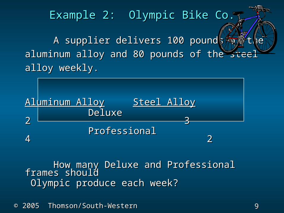
A supplier delivers 100 pounds of theA supplier delivers 100 pounds of the

aluminum alloy and 80 pounds of the steelaluminum alloy and 80 pounds of the steel

alloy weekly. alloy weekly.

Aluminum AlloyAluminum Alloy Steel AlloySteel Alloy

Deluxe Deluxe 2 2 3 3

Professional 4 Professional 4 22

How many Deluxe and Professional frames How many Deluxe and Professional frames shouldshould Olympic produce each week?Olympic produce each week?

Example 2: Olympic Bike Co.Example 2: Olympic Bike Co.

10 10 Slide

Slide



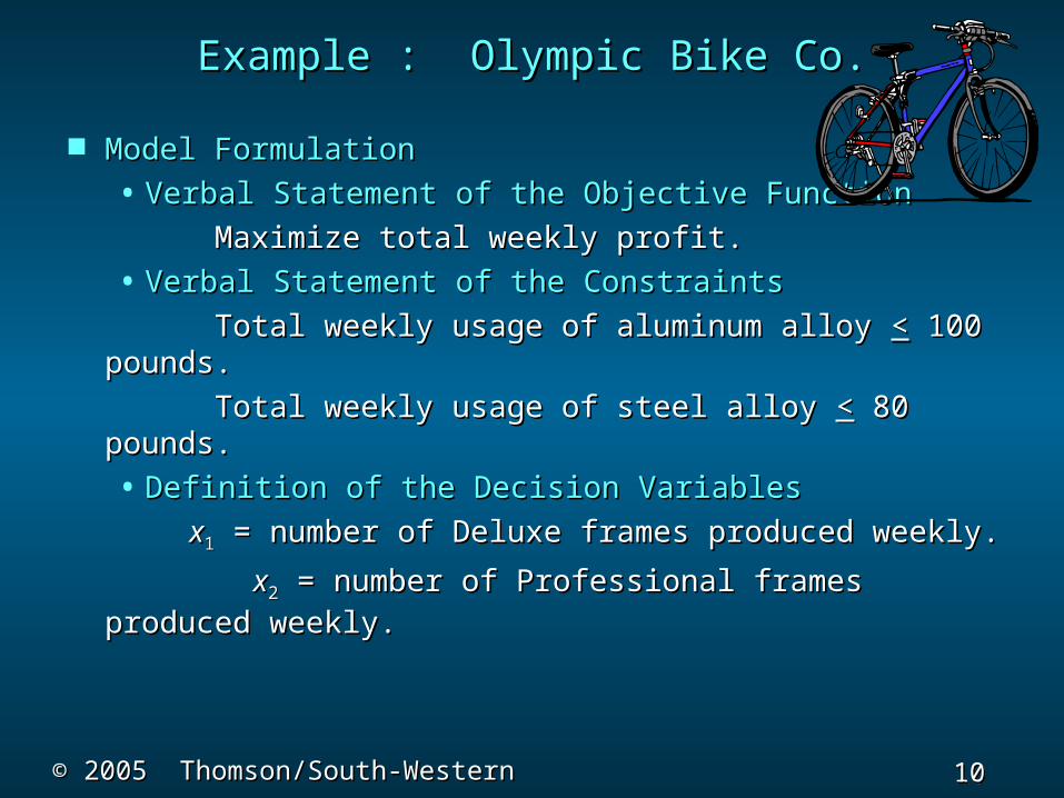
Model FormulationModel Formulation

• Verbal Statement of the Objective FunctionVerbal Statement of the Objective Function

Maximize total weekly profit.Maximize total weekly profit.

• Verbal Statement of the ConstraintsVerbal Statement of the Constraints

Total weekly usage of aluminum alloy Total weekly usage of aluminum alloy << 100 100 pounds.pounds.

Total weekly usage of steel alloy Total weekly usage of steel alloy << 80 pounds. 80 pounds.

• Definition of the Decision VariablesDefinition of the Decision Variables

xx11 = number of Deluxe frames produced weekly. = number of Deluxe frames produced weekly.

xx22 = number of Professional frames produced = number of Professional frames produced weekly.weekly.

11 11 Slide

Slide



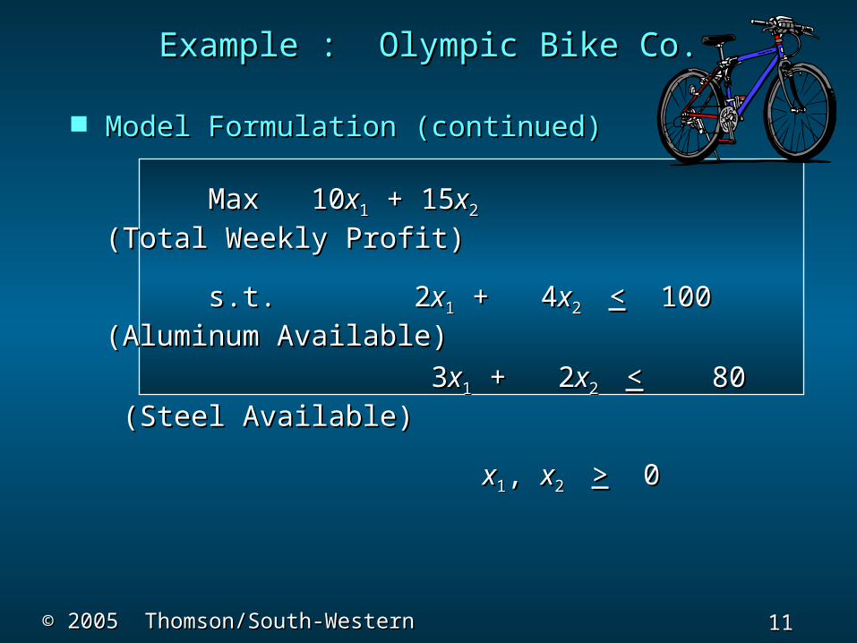
Model Formulation (continued)Model Formulation (continued)

Max 10Max 10xx11 + 15 + 15xx22 (Total (Total Weekly Profit) Weekly Profit)

s.t. 2s.t. 2xx11 + 4 + 4xx2 2 << 100 (Aluminum 100 (Aluminum Available)Available)

33xx11 + 2 + 2xx2 2 << 80 (Steel 80 (Steel Available)Available)

xx11, , xx2 2 >> 0 0

12 12 Slide

Slide



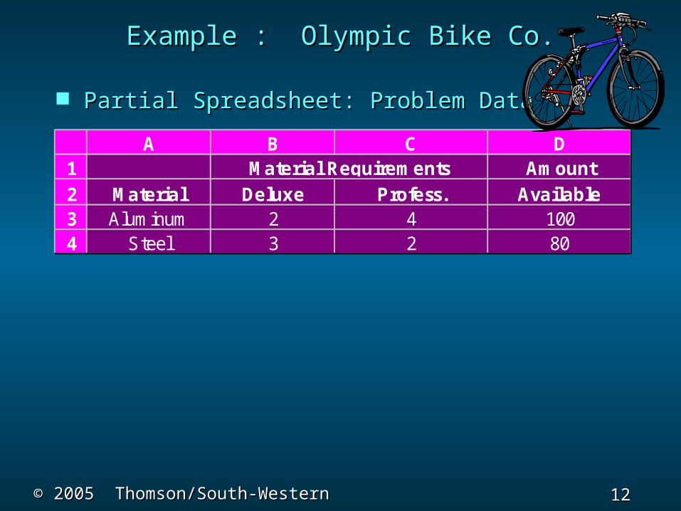
Partial Spreadsheet: Problem DataPartial Spreadsheet: Problem Data

A B C D1 Amount2 Material Deluxe Profess. Available3 Aluminum 2 4 1004 Steel 3 2 80

Material RequirementsA B C D

1 Amount2 Material Deluxe Profess. Available3 Aluminum 2 4 1004 Steel 3 2 80

Material Requirements

13 13 Slide

Slide



Partial Spreadsheet Showing SolutionPartial Spreadsheet Showing Solution

A B C D67 Deluxe Professional8 Bikes Made 15 17.5009

10 412.5001112 Constraints Amount Used Amount Avail.13 Aluminum 100 <= 10014 Steel 80 <= 80

Decision Variables

Maximized Total Profit

A B C D67 Deluxe Professional8 Bikes Made 15 17.5009

10 412.5001112 Constraints Amount Used Amount Avail.13 Aluminum 100 <= 10014 Steel 80 <= 80

Decision Variables

Maximized Total Profit

14 14 Slide

Slide



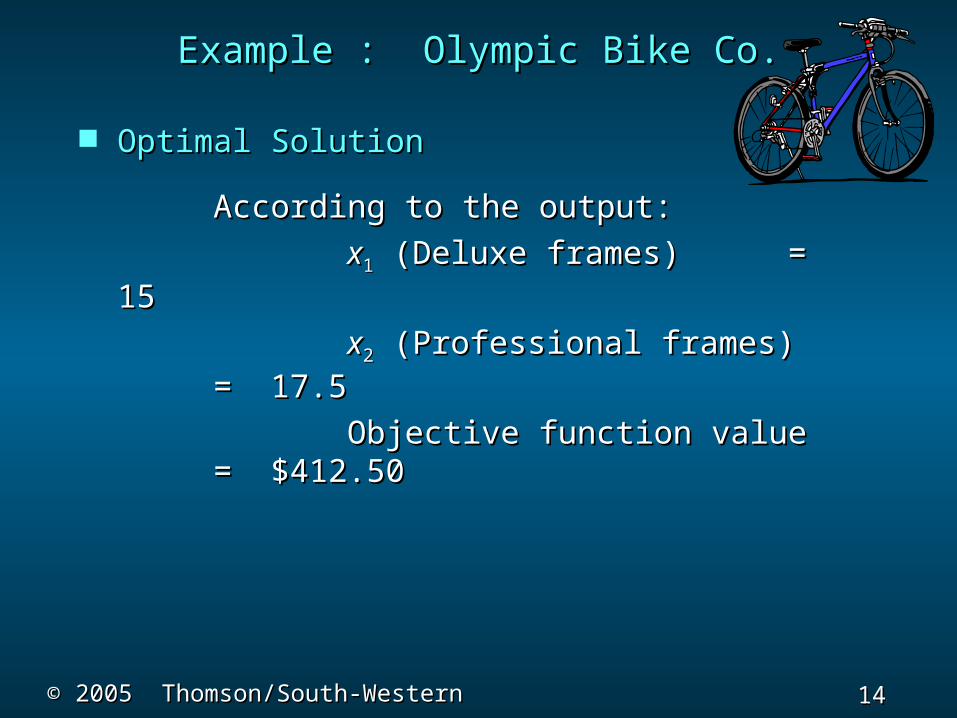
Optimal SolutionOptimal Solution

According to the output:According to the output:

xx11 (Deluxe frames) (Deluxe frames) = 15= 15

xx22 (Professional frames) (Professional frames) = = 17.517.5

Objective function value Objective function value = = $412.50$412.50

15 15 Slide

Slide



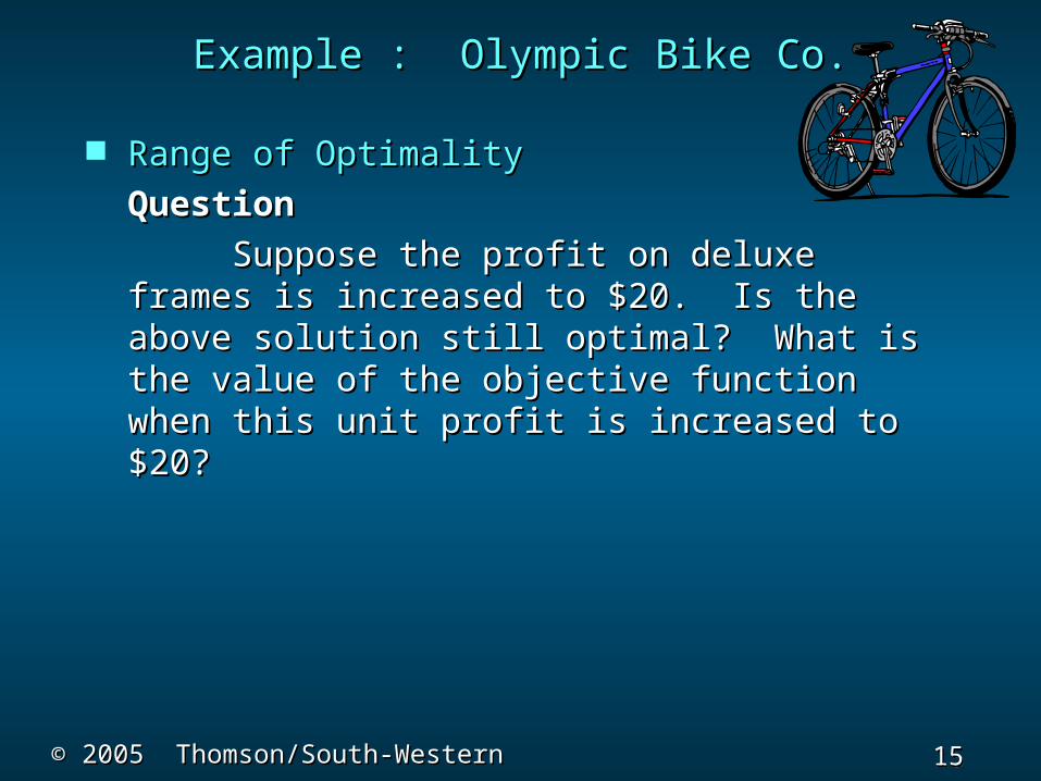
Range of OptimalityRange of Optimality

QuestionQuestion

Suppose the profit on deluxe frames is Suppose the profit on deluxe frames is increased to $20. Is the above solution still increased to $20. Is the above solution still optimal? What is the value of the objective optimal? What is the value of the objective function when this unit profit is increased to function when this unit profit is increased to $20?$20?

16 16 Slide

Slide



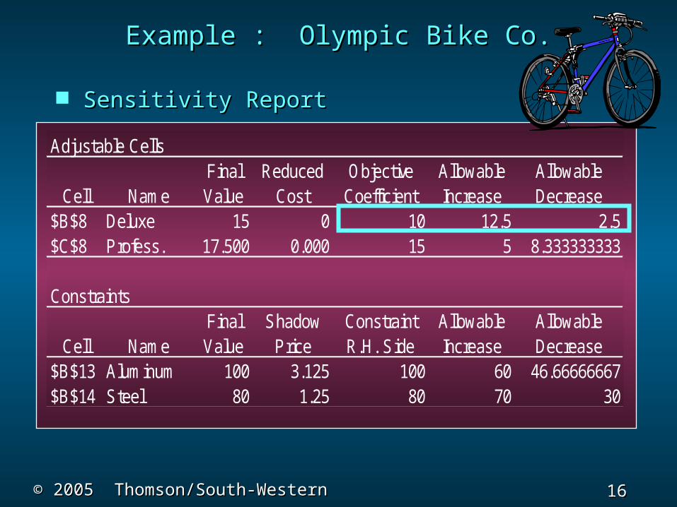
Sensitivity ReportSensitivity Report

Adjustable CellsFinal Reduced Objective Allowable Allowable

Cell Name Value Cost Coefficient Increase Decrease$B$8 Deluxe 15 0 10 12.5 2.5$C$8 Profess. 17.500 0.000 15 5 8.333333333

ConstraintsFinal Shadow Constraint Allowable Allowable

Cell Name Value Price R.H. Side Increase Decrease$B$13 Aluminum 100 3.125 100 60 46.66666667$B$14 Steel 80 1.25 80 70 30

17 17 Slide

Slide




AnswerAnswer

The output states that the solution The output states that the solution remains optimal as long as the objective remains optimal as long as the objective function coefficient of function coefficient of xx11 is between 7.5 and is between 7.5 and

22.5. Since 20 is within this range, the optimal 22.5. Since 20 is within this range, the optimal solution will not change. The optimal profit will solution will not change. The optimal profit will change: 20change: 20xx11 + 15 + 15xx22 = 20(15) + 15(17.5) = = 20(15) + 15(17.5) =

$562.50.$562.50.

18 18 Slide

Slide




QuestionQuestion

If the unit profit on deluxe frames were If the unit profit on deluxe frames were $6 instead of $10, would the optimal solution $6 instead of $10, would the optimal solution change?change?

19 19 Slide

Slide




Adjustable CellsFinal Reduced Objective Allowable Allowable

Cell Name Value Cost Coefficient Increase Decrease$B$8 Deluxe 15 0 10 12.5 2.5$C$8 Profess. 17.500 0.000 15 5 8.33333333

ConstraintsFinal Shadow Constraint Allowable Allowable

Cell Name Value Price R.H. Side Increase Decrease$B$13 Aluminum 100 3.125 100 60 46.66666667$B$14 Steel 80 1.25 80 70 30

20 20 Slide

Slide



AnswerAnswer

The output states that the solution The output states that the solution remains optimal as long as the objective remains optimal as long as the objective function coefficient of function coefficient of xx11 is between 7.5 and is between 7.5 and

22.5. Since 6 is outside this range, the optimal 22.5. Since 6 is outside this range, the optimal solution would change.solution would change.


21 21 Slide

Slide


End of Chapter 3End of Chapter 3

Documents

Advancesensit