Embed Size (px)
Citation preview

AERODYNAMIC ANDAEROACOUSTIC ANALYSIS OF
COUNTER ROTATINGOPEN ROTORS
A thesis submitted to the University of Manchester
for the degree of Doctor of Philosophy
in the Faculty of Science and Engineering
2020
Dale A. Smith
School of EngineeringDepartment of Mechanical Aerospace and Civil Engineering
Contents
Abstract 10
Declaration 11
Copyright 12
Acknowledgements 13
Publications 14
Nomenclature 15
1 Introduction 21
1.1 Description of CROR . . . . . . . . . . . . . . . . . . . . . . . . . . . . . . 21
1.2 Literature Survey . . . . . . . . . . . . . . . . . . . . . . . . . . . . . . . . 23
1.2.1 Blade Sweep . . . . . . . . . . . . . . . . . . . . . . . . . . . . . . . 23
1.2.2 Rotor Trim . . . . . . . . . . . . . . . . . . . . . . . . . . . . . . . . 25
1.2.3 Geometry Modifications . . . . . . . . . . . . . . . . . . . . . . . . 26
1.2.4 CROR Optimisation . . . . . . . . . . . . . . . . . . . . . . . . . . 33
1.2.5 Fore Rotor Trailing Edge Blowing . . . . . . . . . . . . . . . . . . 35
1.2.6 Installation and Shielding . . . . . . . . . . . . . . . . . . . . . . . 35
1.2.7 Summary . . . . . . . . . . . . . . . . . . . . . . . . . . . . . . . . 41
1.3 Objectives of the Thesis . . . . . . . . . . . . . . . . . . . . . . . . . . . . 41
1.4 Thesis Structure . . . . . . . . . . . . . . . . . . . . . . . . . . . . . . . . . 41
2 Aerodynamic Modelling 43
2.1 Low-Order Aerodynamic Modelling . . . . . . . . . . . . . . . . . . . . . 43
2.1.1 Blade Element Momentum Theory . . . . . . . . . . . . . . . . . . 44
2.1.2 Extension to Counter Rotating Open Rotors . . . . . . . . . . . . 47
2.1.3 Rotor-Rotor Interactions . . . . . . . . . . . . . . . . . . . . . . . . 53
2.1.4 2D Aerodynamics . . . . . . . . . . . . . . . . . . . . . . . . . . . 55
2

2.1.5 Model Corrections . . . . . . . . . . . . . . . . . . . . . . . . . . . 55
2.1.6 Rotor Trim . . . . . . . . . . . . . . . . . . . . . . . . . . . . . . . . 56
2.1.7 Model Validation . . . . . . . . . . . . . . . . . . . . . . . . . . . . 57
2.1.8 Sensitivity Analysis . . . . . . . . . . . . . . . . . . . . . . . . . . 63
2.2 High-Order Aerodynamic Modelling . . . . . . . . . . . . . . . . . . . . 70
2.2.1 The Governing Equations . . . . . . . . . . . . . . . . . . . . . . . 70
2.2.2 The HMB3 Solver . . . . . . . . . . . . . . . . . . . . . . . . . . . . 71
2.2.3 Turbulence Closure . . . . . . . . . . . . . . . . . . . . . . . . . . . 73
2.2.4 Meshing Strategy . . . . . . . . . . . . . . . . . . . . . . . . . . . . 75
2.2.5 Model Validation . . . . . . . . . . . . . . . . . . . . . . . . . . . . 87
2.2.6 HMB execution . . . . . . . . . . . . . . . . . . . . . . . . . . . . . 93
2.3 Summary . . . . . . . . . . . . . . . . . . . . . . . . . . . . . . . . . . . . . 94
3 Aeroacoustic Modelling 95
3.1 Rotor Noise Sources . . . . . . . . . . . . . . . . . . . . . . . . . . . . . . 95
3.2 Noise Metrics . . . . . . . . . . . . . . . . . . . . . . . . . . . . . . . . . . 98
3.3 Low-Order Noise Modelling . . . . . . . . . . . . . . . . . . . . . . . . . . 100
3.3.1 Model Validation . . . . . . . . . . . . . . . . . . . . . . . . . . . . 105
3.3.2 Sensitivity Analysis . . . . . . . . . . . . . . . . . . . . . . . . . . 108
3.4 High-Order Noise Modelling . . . . . . . . . . . . . . . . . . . . . . . . . 114
3.4.1 Farassat 1A Code . . . . . . . . . . . . . . . . . . . . . . . . . . . . 114
3.4.2 Model Validation . . . . . . . . . . . . . . . . . . . . . . . . . . . . 116
3.4.3 Effect of Turbulence Model . . . . . . . . . . . . . . . . . . . . . . 118
3.5 Summary . . . . . . . . . . . . . . . . . . . . . . . . . . . . . . . . . . . . . 120
4 A Parametric Study of CROR Noise 121
4.1 Blade Count Investigation . . . . . . . . . . . . . . . . . . . . . . . . . . . 121
4.2 Tip Speed Investigation . . . . . . . . . . . . . . . . . . . . . . . . . . . . 124
4.3 Combined Blade Count and Tip Speed Investigation . . . . . . . . . . . 126
4.4 Open Rotor Optimisation . . . . . . . . . . . . . . . . . . . . . . . . . . . 128
4.4.1 Optimisation Routine . . . . . . . . . . . . . . . . . . . . . . . . . 128
4.4.2 CROR design - Civil Aviation . . . . . . . . . . . . . . . . . . . . . 132
4.4.3 CROR design - General Aviation . . . . . . . . . . . . . . . . . . . 136
4.5 Summary . . . . . . . . . . . . . . . . . . . . . . . . . . . . . . . . . . . . . 139
5 CROR Noise Reduction — Low-Order Analysis 141
5.1 Description of Proposed Configurations . . . . . . . . . . . . . . . . . . . 141
5.2 Locked-Fore Rotor . . . . . . . . . . . . . . . . . . . . . . . . . . . . . . . 144
5.3 Locked-Aft Rotor . . . . . . . . . . . . . . . . . . . . . . . . . . . . . . . . 147
3

5.3.1 Folded Aft Rotor . . . . . . . . . . . . . . . . . . . . . . . . . . . . 1505.3.2 Increased Fore Radius . . . . . . . . . . . . . . . . . . . . . . . . . 151
5.4 Summary . . . . . . . . . . . . . . . . . . . . . . . . . . . . . . . . . . . . . 154
6 CROR Noise Reduction — High-Order Analysis 1556.1 Description of Test Cases . . . . . . . . . . . . . . . . . . . . . . . . . . . . 1556.2 Aerodynamic Analysis . . . . . . . . . . . . . . . . . . . . . . . . . . . . . 1576.3 Aeroacoustic Analysis . . . . . . . . . . . . . . . . . . . . . . . . . . . . . 1676.4 Summary . . . . . . . . . . . . . . . . . . . . . . . . . . . . . . . . . . . . . 175
7 Conclusions and Future Work 1767.1 Conclusions . . . . . . . . . . . . . . . . . . . . . . . . . . . . . . . . . . . 1767.2 Future Work . . . . . . . . . . . . . . . . . . . . . . . . . . . . . . . . . . . 179
A Appendix A - Broadband Noise 180A.1 Trailing-Edge Source . . . . . . . . . . . . . . . . . . . . . . . . . . . . . . 180A.2 Rotor-Rotor Interaction Source . . . . . . . . . . . . . . . . . . . . . . . . 181
Bibliography 184
Word Count (excluding Bibliography, Appendices, Contents, Copyright statement,Declaration): ∼ 39,670
4

List of Tables
2.1 CROR velocity components. . . . . . . . . . . . . . . . . . . . . . . . . . . . 492.2 DLR CROR performance computed using CFD and BEMT model. . . . . . . 622.3 Comparison of works employing Chimera technique for CROR analysis 762.4 Background grid refinement parameters. . . . . . . . . . . . . . . . . . . . . . 812.5 Computed loads for each background grid. . . . . . . . . . . . . . . . . . . . . 822.6 Chimera grid refinement parameters. . . . . . . . . . . . . . . . . . . . . . . . 842.7 Computed loads for Chimera each grid. . . . . . . . . . . . . . . . . . . . . . 85
4.1 CROR design parameters for parametric noise study. . . . . . . . . . . . . . . 1224.2 Operating point parameters. . . . . . . . . . . . . . . . . . . . . . . . . . . . 1224.3 Optimisation design objectives and free variables . . . . . . . . . . . . . . . . 1324.4 Upper and lower limits of free variables for optimisation cases I and II. . . . . 1334.5 Upper and lower limits of free variables for optimisation case III. . . . . . . . . 1334.6 Take-off and Cruise operating parameters. . . . . . . . . . . . . . . . . . . . . 1334.7 Civil aviation optimisation. . . . . . . . . . . . . . . . . . . . . . . . . . . . . 1344.8 Upper and lower limits of free variables for optimisation cases I and II. . . . . 1374.9 Upper and lower limits of free variables for optimisation case III. . . . . . . . . 1374.10 Take-off and cruise operating parameters. . . . . . . . . . . . . . . . . . . . . 1374.11 General aviation optimisation. . . . . . . . . . . . . . . . . . . . . . . . . . . 138
5.1 Operating point parameters. . . . . . . . . . . . . . . . . . . . . . . . . . . . 1435.2 Rotor design parameters. . . . . . . . . . . . . . . . . . . . . . . . . . . . . . 144
6.1 Rotor design parameters. . . . . . . . . . . . . . . . . . . . . . . . . . . . . . 1566.2 Fore and aft rotor setting angles for each configuration. . . . . . . . . . . . . . 1596.3 Computed thrust for each configuration. Target thrust = 6 kN. . . . . . . . . 1596.4 Computed torque and efficiency of each configuration. . . . . . . . . . . . . . 1606.5 Noise levels for each configuration. . . . . . . . . . . . . . . . . . . . . . . . . 168
5

List of Figures
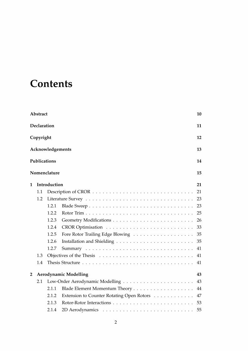
1.1 CROR concepts of the 1980s under flight testing. . . . . . . . . . . . . . . . . 22
1.2 Modern CROR concepts under testing as part of the EU CleanSky SAGEproject [17]. . . . . . . . . . . . . . . . . . . . . . . . . . . . . . . . . . . . . 23
1.3 Three rotors tested in the NASA Lewis tunnel to investigate sweep, fromRef. [23]. . . . . . . . . . . . . . . . . . . . . . . . . . . . . . . . . . . . . . 24
1.4 Iso-surface of Q-criterion showing tip vortex interaction. . . . . . . . . . . . . 26
1.5 Comparison of clipped (F7/A3) and unclipped (F7/A7) CROR directivities,adapted from Ref. [36] . . . . . . . . . . . . . . . . . . . . . . . . . . . . . . 27
1.6 Effect of axial spacing on rotor alone and interaction tones. Adapted fromRef. [34]. . . . . . . . . . . . . . . . . . . . . . . . . . . . . . . . . . . . . . 28
1.7 Cause of increased noise with increased spacing at cruise Mach numbers.Adapted from Ref. [39]. . . . . . . . . . . . . . . . . . . . . . . . . . . . . . . 29
1.8 Protuberance placed on CROR fore rotor, from Ref. [43]. . . . . . . . . . . . . 30
1.9 Airbus AI-PX7 CROR with trailing-edge serrations on the fore rotor, fromRef [50]. . . . . . . . . . . . . . . . . . . . . . . . . . . . . . . . . . . . . . . 31
1.10 Blade geometry and hub configurations studied by Barakos & Johnson andChirico, Barakos & Bown, from Ref. [53]. . . . . . . . . . . . . . . . . . . . . 32
1.11 Optimised CROR designs identified by Grasso et al., blue shows optimisedgeometry against the grey baseline. Adapted from Ref. [58]. . . . . . . . . . . 34
1.12 Full aircraft installation configuration studied by Stuermer, from Ref [67]. . . 36
1.13 Clean Sky WENEMOR project scale aircraft and some of the configurationsstudied, from Ref [80]. . . . . . . . . . . . . . . . . . . . . . . . . . . . . . . 40
2.1 Representation of propeller disc in momentum theory. . . . . . . . . . . . . . 44
2.2 Velocity and force components acting on a blade element. . . . . . . . . . . . . 45
2.3 Momentum theory schematic for CROR. . . . . . . . . . . . . . . . . . . . . 47
2.4 CROR velocity triangles. . . . . . . . . . . . . . . . . . . . . . . . . . . . . . 51
2.5 Workflow for solving CROR BEMT equations. . . . . . . . . . . . . . . . . . 54
2.6 Definition of CROR fore and aft rotor setting angles and rotation senses. . . . 56
2.7 Implemented rotor trimming routine. . . . . . . . . . . . . . . . . . . . . 57
6

2.8 SR2 spanwise geometry. . . . . . . . . . . . . . . . . . . . . . . . . . . . . . 582.9 Comparison of SR2 thrust coefficient. . . . . . . . . . . . . . . . . . . . . . . 582.10 Location of probes and CROR reference frame. . . . . . . . . . . . . . . . . . 592.11 SR2 Axial comparison. . . . . . . . . . . . . . . . . . . . . . . . . . . . . . . 602.12 SR2 Tangential comparison. . . . . . . . . . . . . . . . . . . . . . . . . . . . 612.13 DLR advanced CROR concept (adapted from Ref. [72]) . . . . . . . . . . . . . 612.14 Details of the Rolls-Royce Rig-140 CROR (adapted from Ref. [108]). . . . . . 632.15 Comparison of Rig-140 data at cruise. . . . . . . . . . . . . . . . . . . . . . . 642.16 Discretisation sensitivity analysis. . . . . . . . . . . . . . . . . . . . . . . . . 652.17 Effect of chord data on CROR performance. . . . . . . . . . . . . . . . . . . . 662.18 Detailed performance effect of changes in rotor chord. . . . . . . . . . . . . . . 662.19 Effect of aerodynamic data on CROR performance. . . . . . . . . . . . . . . . 682.20 Effect of aerodynamic data at constant advance ratio. . . . . . . . . . . . . . . 682.21 Effect of aerodynamic data across a range of advance ratios. . . . . . . . . . . 692.22 Chimera localisation . . . . . . . . . . . . . . . . . . . . . . . . . . . . . . . 762.23 Background grid topology. . . . . . . . . . . . . . . . . . . . . . . . . . . . . 782.24 Background grid topology. . . . . . . . . . . . . . . . . . . . . . . . . . . . . 792.25 Blade topology and grid. . . . . . . . . . . . . . . . . . . . . . . . . . . . . . 802.26 Assembled surface grids (every second cell shown). . . . . . . . . . . . . . . . 812.27 Velocity profile comparison for three mesh densities 1R downstream of the rotor. 832.28 Velocity profile comparison for three mesh densities 2R downstream of the rotor. 832.29 Axial velocity along the normal direction from blade suction and pressure
surfaces for medium and fine Chimera grids. Located approximately at 0.75Rat the blade mid-chord with the distance normalised by blade tip chord. . . . . 85
2.30 Comparison of skin friction coefficient for medium and fine Chimera grids. . . 862.31 CFD and experimental normalised axial velocity. . . . . . . . . . . . . . . . . 882.32 CFD and experimental normalised tangential velocity. . . . . . . . . . . . . . 892.33 CFD and experimental normalised radial velocity. . . . . . . . . . . . . . . . 902.34 Normalised axial velocity for each turbulence model. . . . . . . . . . . . . . . 922.35 Normalised tangential velocity for each turbulence model. . . . . . . . . . . . 922.36 Normalised radial velocity for each turbulence model. . . . . . . . . . . . . . . 93
3.1 CROR noise sources. . . . . . . . . . . . . . . . . . . . . . . . . . . . . . . . 963.2 Rotor steady noise characteristics (adapted from [21]). . . . . . . . . . . . . . 963.3 Rotor steady noise characteristics (adapted from [21]). . . . . . . . . . . . . . 973.4 CROR interactions resulting in unsteady loading. . . . . . . . . . . . . . . . 983.5 A-weighting frequency gain. . . . . . . . . . . . . . . . . . . . . . . . . . . . 1003.6 Definition of Observer location. . . . . . . . . . . . . . . . . . . . . . . . . . 1033.7 SRP noise prediction. . . . . . . . . . . . . . . . . . . . . . . . . . . . . . . . 106
7

3.8 Microphone locations for CROR noise validation, adapted from Ref. [164]. . . 107
3.9 Comparison of computed and reported SPL values for SR2 CROR. . . . . . . 107
3.10 Effect of blade thickness on thickness noise. . . . . . . . . . . . . . . . . . . . 109
3.11 Effect of Rotational speed. . . . . . . . . . . . . . . . . . . . . . . . . . . . . 109
3.12 Effect of steady aerodynamic component on peak and EPNL noise levels. . . . 111
3.13 Effect of the unsteady loading component of CROR noise. . . . . . . . . . . . 111
3.14 Harmonic components for steady and unsteady aerodynamics at overhead po-sition, θ = 90. . . . . . . . . . . . . . . . . . . . . . . . . . . . . . . . . . . 112
3.15 Effect of time discretisation. . . . . . . . . . . . . . . . . . . . . . . . . . . . 114
3.16 Blade discretisation for aeroacoustic analysis. . . . . . . . . . . . . . . . . . . 116
3.17 Validation of the high-order noise model for azimuthally averaged polar direc-tivities. . . . . . . . . . . . . . . . . . . . . . . . . . . . . . . . . . . . . . . 117
3.18 Effect of turbulence closure on CROR flyover noise for the noise validation case.119
4.1 Blade counts giving lowest EPNL for all operating points. . . . . . . . . . . . 123
4.2 Blade counts giving highest EPNL for all operating points. . . . . . . . . . . . 124
4.3 Effect of tip speed on the EPNL of the 8×5 combinations at all operating points.125
4.4 Effect of tip speed with increasing aft blade count. . . . . . . . . . . . . . . . . 126
4.5 Effect of tip speed with increasing fore blade count. . . . . . . . . . . . . . . . 127
4.6 Operation of a Genetic Algorithm. . . . . . . . . . . . . . . . . . . . . . . . . 129
4.7 Bernstein polynomial components represented analogously to Pascal’s triangle. 132
4.8 Effect of population size on minimum object value. . . . . . . . . . . . . . . . 134
4.9 Spanwise geometry of optimised civil aviation designs. . . . . . . . . . . . . . 135
4.10 CAD representations of the optimised civil aviation designs. . . . . . . . . . . 136
4.11 Spanwise geometry of optimised general aviation designs. . . . . . . . . . . . 139
4.12 CAD representations of optimised general aviation CROR. . . . . . . . . . . . 140
5.1 Multi-configuration CROR concepts. . . . . . . . . . . . . . . . . . . . . . . 142
5.2 Comparison of noise between baseline CROR and a CROR with locked-foreblade row. CROR is the baseline configuration and inop the locked-rotor con-figuration. . . . . . . . . . . . . . . . . . . . . . . . . . . . . . . . . . . . . . 145
5.3 Comparison of noise between baseline CROR and a CROR with locked-aftblade row. CROR is the baseline configuration and inop the locked-rotor con-figuration. . . . . . . . . . . . . . . . . . . . . . . . . . . . . . . . . . . . . . 148
5.4 EPNL of baseline operative CROR and a CROR with a locked blade row.CROR is the baseline configuration and inop the locked-rotor configuration. . 149
5.5 Comparison of total noise locked-aft and folded-aft rotors for take-off conditions.151
5.6 Effect of increasing radius on locked-aft and baseline CROR configurations. . . 152
8

5.7 Difference in noise between locked-aft and operative CROR for increasingradius for the 6× 4 combination. . . . . . . . . . . . . . . . . . . . . . . . . 153
6.1 Baseline and inoperative configurations. . . . . . . . . . . . . . . . . . . . . . 1566.2 Convergance monitors for CFD simulations (initial transients cropped to show
final periodicity). . . . . . . . . . . . . . . . . . . . . . . . . . . . . . . . . . 1586.3 Azimuthal velocity profiles time-averaged over a single rotation. Vre f is the
reference velocity, equivalent to M = 0.2. . . . . . . . . . . . . . . . . . . . . 1616.4 Computed rotor axial force for each configuration over a single revolution. . . 1616.5 Harmonic content of axial force of operative rotor for each configuration. Note
the axis scale in each sub-figure. . . . . . . . . . . . . . . . . . . . . . . . . . 1636.6 Azimuthal variation of axial velocity x = g
2 downstream the fore rotor. . . . . 1646.7 Azimuthal variation of axial velocity x = g
2 upstream the fore rotor. . . . . . . 1646.8 Contours of axial velocity with iso-surfaces of Q-criterion, Q = 0.2 for each
configuration. . . . . . . . . . . . . . . . . . . . . . . . . . . . . . . . . . . . 1656.9 Microphone locations for aeroacoustic analysis (note: positions not to scale
and not every point shown). . . . . . . . . . . . . . . . . . . . . . . . . . . . 1676.10 A-weighted SPL computed for each configuration. . . . . . . . . . . . . . . . 1686.11 Noise components of the baseline configuration. . . . . . . . . . . . . . . . . . 1696.12 Rotor noise contributions for locked-rotor configurations. . . . . . . . . . . . . 1706.13 Azimuthal directivity of baseline and SRP configuration. . . . . . . . . . . . . 1716.14 Azimuthal directivity of rotor components for locked-rotor configurations. . . . 1726.15 Harmonic components of baseline and SRP configurations at the overhead
position. . . . . . . . . . . . . . . . . . . . . . . . . . . . . . . . . . . . . . . 1736.16 Harmonic components of locked-rotor configurations at the overhead position. . 174
9

Abstract
Due to their potential to significantly reduce aircraft emissions, there is a renewedinterest in Counter Rotating Open Rotors (CROR). However, there are concerns sur-rounding their noise emissions. In an effort to address this, the present work focuseson developing and applying numerical tools to study noise-reducing strategies forCROR. In particular, the work is primarily focussed on the application to generalaviation aircraft.
A number of low-order tools have been developed in order to consider a large de-sign space. The low-order tools are used to undertake a CROR design study utilisingan optimisation routine. A number of CROR designs were identified that successfullyreduced noise at take-off whilst simultaneously meeting a number of other additionaldesign constraints.
A number of novel CROR configurations are proposed to reduce noise in theterminal area. Firstly, it is proposed to lock either the fore or the aft rotor duringtake-off, climb-out and approach conditions, with the operative rotor delivering thetotal thrust. During cruise, the locked rotor is restarted to realise the high efficiencyof the CROR. It is hypothesised that locking a blade row will reduce the interactioncomponent that dominates the CROR noise footprint in the terminal area.
The low-order design tools are first used to investigate the potential of the novelconfigurations over a wide design space. The low-order models identified a numberof blade count combinations offering reductions in noise relative to a baseline CROR.
High-order simulations were subsequently carried out to support these predic-tions. uRANS CFD, coupled to an acoustic solver, was used to confirm the potentialof the proposed concepts. In particular, noise reductions of ∼ 3.6 dB(A) were ob-served for the locked-fore configurations, whilst the locked-aft configuration offered∼ 7.9 dB(A) reductions relative to a baseline configuration. These noise reductionscame at the cost of ∼ 5% penalty in efficiency during take-off. However, the cruiseefficiency remains unchanged.
10

Declaration
No portion of the work referred to in this thesis has beensubmitted in support of an application for another degreeor qualification of this or any other university or other in-stitute of learning.
11

Copyright
i. The author of this thesis (including any appendices and/or schedules to thisthesis) owns certain copyright or related rights in it (the “Copyright”) and s/hehas given The University of Manchester certain rights to use such Copyright,including for administrative purposes.
ii. Copies of this thesis, either in full or in extracts and whether in hard or elec-tronic copy, may be made only in accordance with the Copyright, Designs andPatents Act 1988 (as amended) and regulations issued under it or, where appro-priate, in accordance with licensing agreements which the University has fromtime to time. This page must form part of any such copies made.
iii. The ownership of certain Copyright, patents, designs, trade marks and other in-tellectual property (the “Intellectual Property”) and any reproductions of copy-right works in the thesis, for example graphs and tables (“Reproductions”),which may be described in this thesis, may not be owned by the author and maybe owned by third parties. Such Intellectual Property and Reproductions cannotand must not be made available for use without the prior written permission ofthe owner(s) of the relevant Intellectual Property and/or Reproductions.
iv. Further information on the conditions under which disclosure, publication andcommercialisation of this thesis, the Copyright and any Intellectual Propertyand/or Reproductions described in it may take place is available in the Univer-sity IP Policy (see http://documents.manchester.ac.uk/DocuInfo.aspx?DocID=24420), in any relevant Thesis restriction declarations deposited in the Uni-versity Library, The University Library’s regulations (see http://www.library.
manchester.ac.uk/about/regulations/) and in The University’s policy on pre-sentation of Theses
12

Acknowledgements
I would firstly like to thank Mr Mike Newton for the financial support that hasallowed me to carry out the work presented within the thesis. I would like to thankmy supervisor Dr Filippone for the support in getting me this far. I would liketo acknowledge the assistance given by Research IT, and the use of the HPC Pool.Furthermore, I would also like to acknowledge the use of EPCC’s Cirrus HPC serviceand the N8 regional HPC service. Finally, I wish to thank Prof. Barakos and themembers of the CFD laboratory at the University of Glasgow for the use of the HMB3solver for the present work.
13

Publications
Journal Papers
D. A. Smith, A. Filippone, N. Bojdo, “Noise Reduction of a Counter Rotating OpenRotor Through a Locked Blade Row”, Aerospace Science and Technology, 105637, 2019.D. A. Smith, A. Filippone, G. N. Barakos, “Acoustic Analysis of Counter RotatingOpen Rotors with a Locked Blade Row”, AIAA Journal, 2020.
Papers in Conference Proceedings
D. A. Smith, A. Filippone, N. Bojdo, “Low-Order Multidisciplinary Optimisation ofCounter-Rotating Open Rotors”, Proceedings of the European Rotorcraft Forum, 18-21September 2018, Delft, The Netherlands.D. A. Smith, A. Filippone, G. N. Barakos, “High-Order Modelling of Open Rotors”,Proceedings of the MACE PGR Conference, 26 March 2019, Manchester UK,D. A. Smith, A. Filippone, N. Bojdo, “A Parametric Study of Open Rotor Noise”,Proceedings of the 25th AIAA/CEAS Aeroacoustics Conference, 20-23 May 2019, Delft, TheNetherlands.
Presentations without Proceedings
D. A. Smith, A. Filippone, “Counter Rotating Open Rotors for General Aviation”, UKVertical Lift Network Annual Technical Workshop, 22-23 May 2017D. A. Smith, A. Filippone, G. N. Barakos, “Aerodynamics of an Open Rotor with aLocked Blade Row”, UK Vertical Lift Network Annual Technical Workshop, 08-09 April2019
14

Nomenclature
Abbreviations
BEM Boundary Element Method
BEMT Blade Element Momentum Theory
BET Blade Element Theory
BPF Blade Passage Frequency =NΩ2π
CAA Computational AeroAcoustics
CFD Computational Fluid Dynamics
CROR Counter Rotating Open Rotors
EPNL Effective Perceived Noise Level
SPL Sound Pressure Level
SRP Single Rotation Propeller
Roman Symbols
A Blade element area [m2]
c Blade element chord [m]
c0 Speed of sound [m/s]
cd Blade element drag coefficient [-]
cl Blade element lift coefficient [-]
Ca Blade element axial force coefficient [-]
Cn Blade element normal force coefficient [-]
CP Rotor power coefficient = Pρn3D5 [-]
15

CQ Rotor torque coefficient = Qρn2D5 [-]
CT Rotor thrust coefficient = Tρn2D4 [-]
D Rotor diameter [m]
D Drag acoustic source term [-]
e Specific energy of fluid element [J/kg]
E Total energy (per unit volume) of fluid element [J/m3]
f Frequency [Hz]
fD Chordwise drag coefficient distribution [-]
fL Chordwise lift coefficient distribution [-]
fT Chordwise thickness distribution [-]
Fc Centrifugal force [N]
FFFi, FFFv Invsicid/viscous flux vectors [-]
FT Prandtl’s tip/hub loss factor [-]
g Axial spacing between rotors [m]
GA A-weighting filter gain [-]
j Complex variable,√−1 [-]
J Rotor advance ratio = V∞nD [-]
Jν(Z) Bessel function of order ν and argument Z [-]
k1,k2 Harmonics [-]
kx,ky Chordwise wave numbers representing non-compactness [-]
lre f Reference length [m]
` Turbulent length scale [m]
LA A-weighted SPL [dB]
L Lift acoustic source term [-]
m Mass [kg]
16

m Mass flow rate [kg/s]
M∞ Free-stream Mach number = V∞/c0, [-]
Mt Tip Mach number = ΩR/c0, [-]
Mr Relative Mach number = Vr/c0, [-]
n Rotational frequency [Hz]
nnn Unit normal [-]
N Rotor blade count [-]
p Pressure of fluid element [N/m2]
pre f Reference pressure = 2× 10⁻⁵ [N/m2]
p′ Acoustic pressure [N/m2]
P Rotor power [W]
q Heat flux [W/m2]
Q Rotor torque [N ·m]
r Rotor radius [m]
rx,ry,rz Observer location in x,y, and z cartesian system [m]
R Rotor tip radius [m]
R Magnitude of radiation vector [m]
RRR Vector of flux residuals [-]
Re Reyolds number = ρVre f lre fµ [-]
S Shape function [-]
SSS Source term [-]
Sij Strain rate tensor [m/s]
Spp Far-field broadband noise spectrum [Pa2/Hz]
t Time [s]
tc Thickness to chord ratio [-]
17

T Rotor thrust, Fluid temperature [N],[K]
T Thickness acoustic source term [-]
u,v,w Cartesian velocity component [m/s]
Un, Vn, Wn Normalised cartesian velocity component = (U,V,W)/Vre f [-]
V∞ Free stream velocity [m/s]
V Volume of fluid domain [m3]
V– Cell volume [m3]
Vre f Reference velocity [m/s]
WWW Vector of conserved variables [-]
y+ Non-dimensional wall-distance [-]
z Normalised rotor radius = r/R [-]
Greek Symbols
α Local angle of attack [rad]
β Blade setting angle [rad]
γ+,γ− Pitch gains [-]
δ Relative error [-]
δij Kronecker delta [-]
ε Blade lean angle [rad]
ζ,ζt Computed thrust/torque and required value [N],[N ·m]
η Propulsive efficiency [-]
Θ Angle between unit radiation and normal vectors. [rad]
θ Observer polar angle [rad]
κ Interference coefficient [-]
λ Blade sweep angle [rad]
µ Dynamic viscosity [Ns/m2]
18
ν Induced velocity component [m/s]
ρ Working fluid density [kg/m3]
σ Rotor solidity [-]
σij Viscous stress tensor [N/m]
ϕ Blade azimuth angle [rad]
φ Local inflow angle, observer aziumth angle [rad], [rad]
φε Phase angle due to blade lean [-], [rad]
φλ Phase angle due to blade sweep [-], [rad]
ΨD Fourier transformed chordwise distribution of drag [-]
ΨL Fourier transformed chordwise distribution of lift [-]
ΨT Fourier transformed chordwise distribution of thickness [-]
Ω Rotor rotational speed [rad/s]
Subscripts
[·]h Hub component
[·]i Self-induced component
[·]max Maximum value
[·]mi Mutually-induced component
[·]r Relative component
[·]t Tip component
[·]x Axial component
[·]θ Tangential component
[·]∞ Free-stream component
[·].75 Component at 75% rotor span
[·]1,2 Fore/aft rotor
19

“Wha kens perhaps yet but the warld shall seeThae glorius day when folk shall learn to flee:When, by the powers of steam, to onywhere,Ships will be biggit that can sail i’ the airWi’a as great ease as on the waters nowThey sail, an’ carry heavy burdens too.”
Andrew Scott, 1826
20

Chapter 1
Introduction
The first chapter of this thesis introduces the Counter Rotating Open Rotor (CROR)concept, its benefits and current challenges. A literature survey has been carried outto identify the state-of-the-art in tackling these challenges from which the basis ofthe present work has been formed. A description of the motivations follows before asummary of the work carried out is presented.
1.1 Description of CROR
With increasing environmental pressure on the aviation industry, there has been arenewed interest in the CROR concept of late. The CROR comprises two blade rowsrotating in opposite directions around a common shaft. The renewed interest comesas a consequence of the increased efficiency relative to turbofan technologies [1, 2,3, 4]. The improved efficiency results from the counter-rotation of the aft rotor as itremoves the residual swirl imparted onto the flow by the fore rotor. Additionally,without the drag of a duct and a higher by-pass ratio, the CROR performance isfurther improved.
The CROR concept and its benefits have been studied since the early days ofaviation (see, e.g. Ref. [5, 6]). However, the oil crisis of the 1980s perhaps saw themost significant developments in CROR technology with a period of intense researchaimed at delivering a commercial engine [7]. CROR development in this period re-sulted in two concepts to the flight test stage, Figure 1.1, see Ref. [8, 9]. However,with a number of technical issues still to overcome and a drop in oil prices, CRORdevelopment was subsequently scaled back, and a commercial engine was never pro-duced.
With an increasing awareness of aviation’s environmental impact, the CROR con-cept has once again come to light. The CROR concept has been the focus of intenseresearch over the past decade, with current efforts focussed on addressing a number
21

22 CHAPTER 1. INTRODUCTION
of challenges to make the CROR commercially realisable. Figure 1.2 shows state-of-the-art concepts currently under testing.
(a) General Electric UnDucted Fan, adapted from [10] (b) Pratt & Whitney/Allison GearedOpen Rotor, adapted from [11]
Figure 1.1: CROR concepts of the 1980s under flight testing.
Whilst general aviation aircraft (light propeller-driven aircraft with a maximumtake-off mass < 8,618 kg) may not have such a significant environmental impact ascivil aircraft, there is increasing focus on reducing their emissions [12, 13]. Further-more, while the endeavours of most current CROR research remains focussed oncivil aviation aircraft, the use of CROR in general aviation is receiving attention froma number of general aviation engine manufacturers [14]. Despite the difference inaircraft class, there is a great deal of commonality between the underlying physicsof the CROR in each case. Furthermore, there will be overlap in the challenges andtheir solutions between applications to both classes of aircraft.
The increasing environmental pressures have also inspired further propulsionconcepts. In particular, there is a great deal of interest in electrifying flight, eitherfully or intermediately, in a hybrid configuration. The use of two combined pow-erplants lends itself naturally to CROR applications. Hybridisation may be morepromising for general aviation class aircraft where the power requirements are per-haps more realisable with the current state-of-the-art or near-future hybrid technolo-gies. Not only does hybridisation offer even greater reductions in emissions, but theindependent control also offers greater safety during the take-off segment.
Despite the promise of increased efficiency, there remains a number of technicalissues to overcome before the adoption of the CROR as a conventional propulsionsystem. For example, installation and aircraft integration, certification and noise allpresent challenges for the modern CROR [15, 16]. Furthermore, these challenges arenot necessarily commensurate with increases in efficiency. The work presented inthis thesis is concerned with the challenges surrounding CROR noise. In particular,

1.2. LITERATURE SURVEY 23
the focus is on developing tools to evaluate CROR designs and novel concepts thatoffer reduced CROR noise without significantly affecting performance. The currentwork primarily deals with general aviation. However, the methods used and theconclusions drawn are not exclusively limited to this class of aircraft.
(a) (b)
Figure 1.2: Modern CROR concepts under testing as part of the EU CleanSky SAGEproject [17].
1.2 Literature Survey
The previous section has identified that noise remains a pertinent issue for CROR.In this section, the open literature is reviewed, bringing together current knowledgeand concepts related to the reduction of CROR noise. The aim of this is, therefore,to identify the most significant noise source and hence the area to explore to signifi-cantly reduce CROR noise. The literature survey is divided into several sub-sections,grouping the various noise-reducing concepts or technologies.
A number of studies have identified several general principles for the designof low-noise CROR [15, 18, 19, 20]. These design philosophies include increasedaxial spacing, aft rotor clipping and blade sweep, to name but a few. However,the main focus is on reducing the interaction source. To proceed, a number of theseconcepts are further explored in addition to discussing some more advanced conceptsto reduce CROR noise.
1.2.1 Blade Sweep
For rotors with transonic tip speeds, introducing blade sweep is a well-knownmethod for reducing rotor noise [21]. For lower tip speeds, the effect of sweep isless significant. Noise reductions due to sweep comprise two sources. Firstly, sweephas the effect of reducing the relative Mach number along the span (analogous to

24 CHAPTER 1. INTRODUCTION
swept wings), and hence reducing the strength of the quadrupole source. Secondly,sweeping back successive blade elements results in a de-phasing effect between bladesections [18].
Experimental studies have demonstrated significant noise reduction by the use ofblade sweep for high tip speeds. For example, Dittmar, Jeracki & Blaha [22] comparedthe unswept SR2 with the swept SR1-M and SR3 rotor blades up to supersonic tipspeeds in the NASA Lewis 8× 6 ft wind tunnel. Figure 1.3 shows the three rotorswith progressively increasing levels of sweep. The authors demonstrated that bothswept rotors offered significant noise reductions compared to the SR2 rotor, with theSR3, the most highly swept, offering the most substantial reductions in noise. Thesame conclusions were made by Dittmar [23] using the numerical acoustic model ofFarassat [24, 25, 26].
Figure 1.3: Three rotors tested in the NASA Lewis tunnel to investigate sweep, fromRef. [23].
With regards to CROR, blade sweep will have the same effect for the self-noise ofeach rotor. However, sweep may also affect the interaction between blade rows, inparticular, the wake and tip vortex development. Simonich, McCormick & Lavrich [27]carried out an experimental investigation on the interaction of a swept stationaryvane upstream of a rotating blade. For the case of the aft-swept vane, the leading-edge vortex∗ moved outboard towards the tip, coalescing with the tip vortex andresulting in a greater interaction component. On the other hand, for the forward-swept vane, the leading-edge vortex moved inboard and remained distinct from thetip vortex, resulting in a reduced interaction component compared to the aft-sweptvane.
∗The high loading at take-off conditions results in separation at some spanwise location along theleading-edge. This separated flow subsequently reattaches along the chord creating an area of highrecirculation and is known as a leading-edge vortex.

1.2. LITERATURE SURVEY 25
While blade sweep may be used to reduce rotor noise, it must be carefully con-sidered when applied to CROR for its effect on the interaction noise component.Furthermore, the benefits of sweep are only realised for high tip speeds. Therefore,in the case of general aviation CROR, sweep perhaps may not be of great importancewith regards to noise reduction.
1.2.2 Rotor Trim
It is possible to trim a CROR to meet the thrust or torque requirements of a givenflight condition with a combination of fore and aft rotor speed and setting angles.Therefore, there is more than one combination of rotor speed and setting angle todeliver the required thrust. In addition to delivering the aircraft thrust or torque, thegiven combination must also satisfy low-noise requirements.
Zachariadis & Hall [28] investigated changes to setting angles and rotor speedto improve CROR efficiency and noise at take-off conditions. For the given configu-ration, the authors found that the baseline trim settings resulted in a highly loadedfore rotor with flow separation in some regions. The setting angles were reduced todecrease the high incidence, while the rotor speed was increased to maintain the re-quired thrust. The new trim settings resulted in improved aerodynamic performance.While the increased rotational speed increased self-noise, the improved aerodynamicperformance reduced the interaction noise and subsequently, the total CROR noise.
In addition to controlling the self-noise, the rotor speed has a significant effect onthe interaction noise. Aside from the aerodynamic effects on the interaction noise, therotor speed can affect the acoustic interaction [29, 30]. The acoustic interaction is theconstructive and destructive addition of the acoustic pressure signals from fore andaft rotors. Therefore, careful control of rotor speed may result in greater destructiveaddition and hence lower total noise. However, this has to be balanced with theresulting aerodynamic effects.
CROR can be trimmed to meet the aircraft requirements by a number of configu-rations: equal torque ratio, Q2
Q1= 1, equal thrust ratio, T2
T1= 1, or unequal thrust and
unequal torque ratios. Delattre & Falissard [31] investigated the aerodynamic andaeroacoustic effects of fore and aft rotor torque ratio. A total thrust was maintainedby adjusting blade setting angles. Delattre & Falissard found that an increase intorque ratio resulted in a reduction in the emitted SPL across polar directivities. Theincrease in torque ratio resulted in a reduction in the fore rotor loading and hence itscorresponding wake deficit. Therefore, the interaction with the rear row was reducedand resulted in a lower interaction noise component. The total noise was reduceddue to the significance of the interaction component at take-off. An overall increasein propulsive efficiency also accompanied the reduction in noise.

26 CHAPTER 1. INTRODUCTION
The method of trimming the CROR rotors to deliver the required aircraft thrustor torque has been found to have a significant effect on the resulting noise. Therefore,optimisation of setting angles and rotational speeds can ensure reduced noise whilstsatisfying the aircraft loading requirements.
1.2.3 Geometry Modifications
Aft Rotor Clipping
As the tip vortex from the fore rotor is trailed backwards, it impinges on the aft ro-tor, Figure 1.4. This interaction results in an unsteady loading component and henceunsteady noise source on the aft row. Clipping, the reduction of the aft rotor radius,can reduce CROR noise by minimising the tip vortex interaction. The vena-contractaof the tip vortex can be estimated to determine the level of clipping required. How-ever, the behaviour of the tip vortex will change as a result of loading and non-axialflight. Therefore, across all operating points, the properties of the tip vortex must bewell understood. Clipping the aft rotor results in a reduced blade area. Increasingthe chord or rotational speed can be used to offset the increased loading.
Figure 1.4: Iso-surface of Q-criterion showing tip vortex interaction.
Peters & Spakovszky [32] attempted to isolate the various interaction noise sourcesnumerically. By considering the noise from the aft rotor in the 90-100% span region,the tip vortex interaction component was isolated. Peters & Spakovszky found thatthe tip vortex interaction component could be as important as the viscous wake com-ponent. It was also subsequently shown that a redesigned CROR with a reducedaft rotor (amongst other design changes) resulted in reduced noise and a significantreduction in the tip vortex interaction component.

1.2. LITERATURE SURVEY 27
Using the NASA Lewis 9 × 15 ft anechoic wind tunnel, Woodward [33] inves-tigated the acoustic performance of an advanced CROR design (F7/A7) at take-offconditions. In a subsequent analysis of a similar design with a 25% reduced aftrotor radius, Woodward & Gordon [34] investigated the effects of clipping. The au-thors found a considerable reduction in noise with the clipped aft rotor. Dittmar& Stang [35] conducted a similar experiment at cruise conditions. Dittmar & Stangalso found that clipping was successful in reducing CROR noise at cruise. Noise re-ductions resulted from a reduction of aft tip speed in addition to a reduction in theinteraction tones as the aft rotor was below the vena-contracta of the fore rotor tipvortex.
Majjigi, Uenishi & Gliebe [36], observing the significant noise reduction achievedwhen clipping the aft rotor, Figure 1.5, noted the importance of accounting for the tipvortex interaction component when numerically modelling CROR interaction noise.From experimental and empirical results, Majjigi, Uenishi & Gliebe developed a tipvortex interaction model that was able to capture the effects of clipping and tip vortexinteraction. This problem has been tackled by a number of authors, including morerecently by Kingan & Self [37] and Quaglia et al. [38].
Observer Angle [deg]
SP
L [
dB
]
60 80 100 120 14085
90
95
100
105
110
No ClippingClipping
Figure 1.5: Comparison of clipped (F7/A3) and unclipped (F7/A7) CROR directivities,adapted from Ref. [36]
Clipping of the aft rotor has been identified as a method for reducing the interac-tion of the fore tip vortex and the aft rotor, and hence the resulting interaction noise.However, the properties of the tip vortex at all flight conditions must be understoodto ensure the rotor has sufficient clipping to realise its benefits.

28 CHAPTER 1. INTRODUCTION
Axial Spacing
Both potential and wake interactions decay with increasing distance. Therefore,the axial spacing between blade rows is an important design consideration. As theaxial distance increases, the viscous wake from the fore rotor has a greater time tomix, resulting in a weaker wake with a lower velocity deficit. The result of thisweaker wake is a reduction in the interaction noise source [19].
The effect of axial spacing was studied experimentally by Woodward [33] at take-off conditions. Woodward found that increasing the axial spacing had a positiveimpact, resulting in a reduction of the noise. Woodward & Gordon [34] performeda similar study with a clipped aft rotor. Comparing their study with that of Wood-ward [33], the authors found that the clipped rotor was more sensitive to changes inaxial distance. Figure 1.6 compares the results from both studies to demonstrate this.The unclipped rotor is affected by both the tip vortices and viscous wake of the forerotor. On the other hand, the clipped rotor is only affected by the viscous wake. Theincreased sensitivity of the clipped rotor results from the fact that the viscous wakedecays more rapidly than the tip vortex.
Axial Spacing, g/D1 []
SP
L [
dB
]
0.15 0.2 0.25110
115
120
125
130
135
F7/A3F7/A7
BPF1
BPF2
BPF1+BPF
2
2BPF1+BPF
2
Figure 1.6: Effect of axial spacing on rotor alone and interaction tones. Adapted fromRef. [34].
Dittmar [39] studied the effects of spacing in the NASA Lewis 8 × 6 ft tunnelfor a CROR blade pair at cruise conditions and observed some interesting results.Whilst the expected trends were observed for a wind tunnel speed of Mach 0.8, theexpected trends were not observed for the reduced tunnel speeds of Mach 0.76 andMach 0.72. For each wind tunnel speed, the setting angle was fixed. Therefore, thereduced speed resulted in an increased inflow angle and hence a greater loading on

1.2. LITERATURE SURVEY 29
each blade. As a result, the wake contraction is greater, and the tip vortex has agreater impact area on the aft row. Despite the weakening due to increased axialspacing, the increased effect of the tip vortex interaction resulted in increased noiselevels. This mechanism is demonstrated in Figure 1.7. The variation in conclusionsfound with increasing spacing demonstrates the complex interaction found in CROR.Furthermore, it highlights the coupling of clipping and axial spacing.
(a) M = 0.8
(b) M = 0.76
(c) M = 0.72
Figure 1.7: Cause of increased noise with increased spacing at cruise Mach numbers.Adapted from Ref. [39].
While the axial spacing has a significant effect on the wake and tip vortex inter-action, it may also be important for the potential interactions. Parry [40] and Parry &Crighton [41] found that potential interactions were the dominant interaction sourcewhen predicting the noise of the Fairey Gannet aircraft. The low blade count of theFairy Gannet CROR blade pair suggests the potential interactions will be significantfor general aviation class aircraft. Similarly to the wake components, the potentialinteractions will decay with increasing axial spacing. Therefore, increased spacingshould also reduce the potential interaction noise source.
In the development of modern CROR designs, there has been a focus on increasedspacing to reduce CROR noise. For example, Peters & Spakovszky [32] describedthe use of increased spacing (amongst other measures) to reduce both wake andpotential interaction noise sources of an advanced CROR design. In describing the

30 CHAPTER 1. INTRODUCTION
collaborative design of a modern CROR, Van Zante [4] described the noise-reducingbenefit of increased axial spacing. However, Van Zante also discussed the need tooptimise this spacing. Increasing the spacing results in the tip vortex being allowedto contract more before meeting the aft rotor, and may result in impingement withthe aft rotor. The optimisation of spacing, taking into account the aft clipping, wasalso discussed by Khalid et al. [42].
It has been established that increasing the axial spacing may be beneficial in re-ducing both potential and wake interaction noise sources. However, the increasedspacing may result in a greater tip vortex interaction. Furthermore, aerodynamicperformance or installation restrictions may limit the axial spacing.
Blade Shape Modifications
In an attempt to reduce the wake interaction noise, Delattre & Falissard [43] andDelattre et al. [44] investigated the effect of placing a small protuberance on theleading-edge of the fore rotor of the Onera HTC5 CROR [45]. The concept aimedto modify the wake structure from the fore rotor and reduce its impact on the aftrotor. Using the Onera elsA CFD solver [46, 47, 48], Delattre & Falissard and Delattreet al. performed a numerical analysis of a CROR with a fore blade modified witha small protuberance at the 80% span location, Figure 1.8. The authors found thatthe protuberance had a minimal impact on the CROR performance at take-off andpractically no effect at cruise conditions.
Figure 1.8: Protuberance placed on CROR fore rotor, from Ref. [43].
The noise produced by each configuration at take-off conditions was studiedbased on the aerodynamic computations. The authors found that the modified CRORhad reduced noise levels for upstream and downstream (from the overhead position)polar directivities. Additionally, the protuberance also caused a reduction in thedominant interaction harmonics.
The observed noise reduction due to the protuberance arises due to a weakeningof the tip vortex. Considering the unmodified configuration, the high loading of the
1.2. LITERATURE SURVEY 31
fore rotor results in the formation of a leading-edge vortex [28, 49]. The small pro-tuberance acts to prevent the merging of the leading-edge vortex with the tip vortex,resulting in two weaker co-rotating vortices leaving the fore row. The interaction ofthe two weaker vortices results in a reduced interaction with the aft rotor and hence,a reduction in noise.
While Delattre & Falissard [43] and Delattre et al. [44] did not investigate theacoustic effects of the protuberance at cruise, due to the leading-edge vortex beingweaker under cruise conditions, it is hypothesised that this concept would have littleimpact on the noise during cruise conditions.
Recall that control of the leading-edge vortex has also been discussed by Simonic,McCormick & Lavrich [27], however, in terms of blade sweep. Forward or backwardsweep was found to move the leading-edge vortex inboard or outboard respectively.Additionally, Khalid et al. [42] discussed additional camber and modified thicknessto prevent the roll-up of the leading-edge vortex.
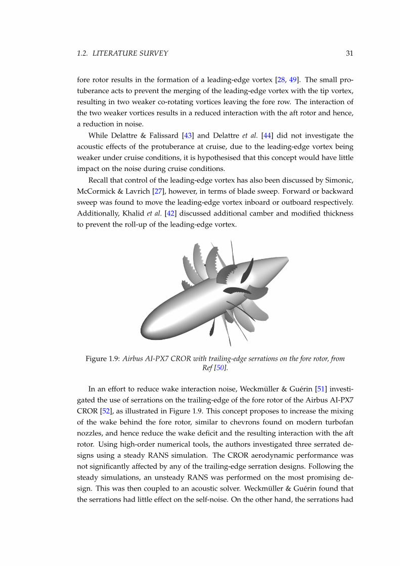
Figure 1.9: Airbus AI-PX7 CROR with trailing-edge serrations on the fore rotor, fromRef [50].
In an effort to reduce wake interaction noise, Weckmuller & Guerin [51] investi-gated the use of serrations on the trailing-edge of the fore rotor of the Airbus AI-PX7CROR [52], as illustrated in Figure 1.9. This concept proposes to increase the mixingof the wake behind the fore rotor, similar to chevrons found on modern turbofannozzles, and hence reduce the wake deficit and the resulting interaction with the aftrotor. Using high-order numerical tools, the authors investigated three serrated de-signs using a steady RANS simulation. The CROR aerodynamic performance wasnot significantly affected by any of the trailing-edge serration designs. Following thesteady simulations, an unsteady RANS was performed on the most promising de-sign. This was then coupled to an acoustic solver. Weckmuller & Guerin found thatthe serrations had little effect on the self-noise. On the other hand, the serrations had

32 CHAPTER 1. INTRODUCTION
a greater benefit with increasing frequency. An OASPL reduction of 0.2 dB resulted.The authors argued that the poor overall reduction was a result of the weaker thanexpected mixing process and the dominance of the tip vortex interaction cloudingany noise reductions resulting from the serrations [3].
Jaron et al. [50] later revisited the serrated blade concept. To identify a design withgreater noise reductions in terms of serration count and depth, Jaron et al. utilisedan evolutionary optimisation routine. Using a steady RANS approach coupled to anacoustic solver, Jaron et al. found a design offering up to 1 dB gains over the baselineAirbus AI-PX7 CROR with little impact on the aerodynamic performance. However,the design was on the border of the optimiser limits of serration depth, suggesting adesign with lower noise may exist.
While the use of serrations on the fore rotor trailing-edge was shown to offerreduced noise compared to a baseline, the manufacturing complexity of such a designmust be further considered against the acoustic benefit. Furthermore, the conceptshould be experimentally studied to verify its performance.
Barakos & Johnson [53] studied a number of blade and hub concepts. In partic-ular, three concepts were studied: (i) a staggered blade concept, where every secondblade was axially displaced aft-wards; (ii) an unequally spaced concept, where bladesare azimuthally unequally spaced; (iii) blades with an off-loaded tip, increased pitchwith a reduced twist at the tip. These concepts are illustrated in Figure 1.10.
(a) Staggered rotor, baseline isgiven in pink, staggered in purple
(b) Unequally spaced, baseline inpink, unequally spaced in blue
(c) Off-loaded tip, baseline in red,off-loaded shown in green
Figure 1.10: Blade geometry and hub configurations studied by Barakos & Johnson andChirico, Barakos & Bown, from Ref. [53].
Barakos & Johnson used the HMB CFD solver to compare the three concepts toa baseline design. From the CFD computations, the near-field acoustic impact ofeach configuration was compared. The authors found that there was no significant

1.2. LITERATURE SURVEY 33
difference in the aerodynamic performance between each configuration. The off-loaded tip configuration reduced noise levels considerably. On the other hand, thestaggered and unequally spaced concepts were shown to introduce sub-harmonics,spreading the tones over a greater range of frequencies and thus changing the soundquality. Nonetheless, the overall sound energy increased compared to the baseline.
This study was later extended by Chirico, Barakos & Bown [54], considering theeffects of these configurations on interior cabin noise. The authors observed similartrends to those reported by Barakos & Johnson [53]. However, the differences betweenthe three configurations reduced with respect to the cabin noise predictions.
The studies performed on the blade and hub configurations have shown that theoff-loaded tip can reduce the resulting noise. On the other hand, the alternativehub configurations showed higher sound energy. The authors studied these conceptsfor near-field and cabin noise. However, it would be interesting to explore thesefurther in the far-field to investigate their community noise impacts. Furthermore,the predictions were made for a Single Rotation Propeller (SRP) and would, therefore,require further analysis for CROR applications.
1.2.4 CROR Optimisation
Increases in computational power have allowed for the development of optimisa-tion routines employing high-fidelity analysis tools. To this end, a number of workshave utilised optimisation tools to target designs towards low-noise while satisfying,amongst others, aircraft thrust and propulsive efficiency requirements.
Lepot et al. [55] and Schnell et al. [56] described the CROR optimisation investi-gated by a number of agencies in the framework of the European DREAM project.The works described the optimisation of a modern CROR based on maximising effi-ciency at the top of climb whilst simultaneously minimising take-off noise. In addi-tion to this, geometrical and structural constraints had to be satisfied. The optimisa-tion utilised an evolutionary algorithm coupled to a steady RANS solver to identifypromising designs. Pseudo-acoustic criteria, namely mean-flow properties of the forerotor wake, were used to evaluate the fitness in terms of noise. The most promisingdesigns were then further studied with unsteady RANS simulations coupled to anacoustic solver. The optimisation identified a design that could reduce noise overmost of the polar directivity at take-off while also meeting the design constraints.The authors noted that the structural constraints were the most limiting to the de-sign. Additionally, the staggering, leading- and trailing-edge profiles and spanwiseloading were reported to have the most significant impact on the optimisation.
Villar, Lindblad & Andersson [57] used an Evolutionary Algorithm to optimisethe efficiency of a CROR at the top of climb. The performance of each design was

34 CHAPTER 1. INTRODUCTION
evaluated from CFD simulations. However, to reduce the number of CFD evaluations,a meta-modelling approach was used. The optimisation, based on aerofoil parametri-sation, identified a design with improved performance relative to the baseline. Whilstthis work does not consider the aeroacoustic impact of the CROR, the meta-modelapproach presents an interesting methodology to reduce the computational cost ofoptimisation studies utilising high-order tools.
Grasso et al. [58] performed a multi-disciplinary, multi-objective optimisation of aCROR. An Evolutionary Algorithm, coupled to a meta-model to decrease computa-tional cost by reducing the number of executions of the numerical models, was usedto identify high performing designs that maximised isentropic efficiency while re-ducing sound power level. Optimisations were carried out on blade profile shape aswell as spanwise sweep and lean. The optimisation was also subject to structural con-straints. RANS CFD, coupled to an analytical acoustic code, was used to compute theaerodynamic performance and tonal and broadband noise sources. The authors iden-tified a number of promising designs along the Pareto front. However, aerodynamicand aeroacoustic objectives were found to be competing. Figure 1.11 compares thedesigns giving the highest efficiency and lowest noise. Low-noise designs resultedfrom increased spacing and reduced chord to reduce the wake deficit. Low-noisedesigns also featured sweep and lean to de-phase radial contributions. Sweep andlean were also used on the high-efficiency designs bringing the blade tips together.
(a) Design identified with highest efficiency (b) Design identified with lowest noise
Figure 1.11: Optimised CROR designs identified by Grasso et al., blue shows optimisedgeometry against the grey baseline. Adapted from Ref. [58].
The use of optimisation routines has shown the ability to identify CROR designswith reduced noise. However, the objective of low-noise is not commensurate withthe objective of high-efficiency. The studies found in the open-literature used a com-bination of high-order methods. However, restraints on computational cost required
1.2. LITERATURE SURVEY 35
simplifications of the physics (the use of steady simulations for an inherently un-steady problem), or limitations on the design space. On the other hand, the use ofmeta-models seems a promising method for reducing the computational cost. De-spite all this, optimisation of the CROR design shows the potential to design a CRORwith low-noise whilst simultaneously meeting further design constraints.
1.2.5 Fore Rotor Trailing Edge Blowing
Further to the use of passive concepts to reduce CROR noise, active concepts havealso demonstrated potential noise reductions. Akkermans, Stuermer & Delfs [59, 60,61] performed a numerical investigation on the ability of trailing-edge blowing toreduce CROR noise at take-off. The concept aims at reducing the wake deficit fromthe fore rotor, and hence the interaction with the aft row, by the injection of airalong the trailing-edge across the blade span. Whilst the concept was shown to makea significant impact in reducing the wake deficit while maintaining aerodynamicperformance, it was unsuccessful in reducing CROR noise. Insufficient clipping of theaft rotor resulted in tip vortex interaction dominating the noise emissions. Therefore,any gains from the trailing-edge blowing, which does not impact the tip vortex, werenot realised.
A later numerical study by Akkermens, Stuermer & Delfs [62, 63] realised thenoise benefits of the trailing-edge blowing concept using an aft rotor with increasedclipping. Again, the trailing-edge blowing significantly reduced the wake deficit atminimal aerodynamic cost (in fact an efficiency gain was observed for the fore rotor).The use of trailing-edge blowing resulted in reduced noise levels across most polardirectivities. The noise reductions resulted from a more pronounced effect on the in-teraction tones, in contrast to the minimal impact it had on the self-tones. Comparedto the study by Akkermans, Stuermer & Delfs, the removal of the tip vortex interac-tion component allowed the noise reduction to be more easily observed. A reductionof 1 dB was demonstrated at the overhead position, whilst up- and downstream di-rectivities showed a maximum of 5 dB reduction relative to the baseline.
To date, only numerical studies have investigated the trailing-edge blowing con-cept. Therefore, the predicted noise reductions need to be experimentally verified.Furthermore, as the mass flow of air will likely be taken as bleed from the engine,the cost in terms of additional fuel consumption must be well understood.
1.2.6 Installation and Shielding
Installation of a rotor on an aircraft can present a vastly distorted flowfield incomparison to the uniform inflow of the idealised isolated case. For example, in-stallation at incidence and boundary layer ingestion both introduce some distortion

36 CHAPTER 1. INTRODUCTION
to the flow. In particular, pylon installation has received significant attention withregards to CROR installation. In pylon mounted rotors, where the pylon is upstreamof the rotor (which is the typical configuration of modern CROR), the wake from thepylon results in periodic changes in incidence and hence a periodic loading on therotor. This unsteady loading then results in an unsteady noise source. The result-ing noise is analogous of stator-rotor interactions, with the upstream stator havinga single blade. The resulting noise will be of mode ν = k2 − k1N1 and of frequencyk1N1n1, where k1 and k2 are all integers, n1 is the rotor rotational frequency and N1 isthe fore rotor blade count. The noise will, therefore, generate tones at the front rotorBlade Passage Frequency (BPF)†.
The installation effects of pylon mounted CROR has been studied by a number ofauthors. Stuermer & Yin [64], using the DLR TAU CFD code [65] and APSIM acousticcode [66], studied the installation effects of a pylon mounted 10× 8 CROR‡ at bothtake-off and cruise conditions. Stuermer & Yin observed that at cruise, the pylon hada significant impact on the rotor alone tones of both fore and aft rotors, resulting inincreased noise levels in the up- and downstream directions. At take-off, the effectwas less pronounced on the aft rotor. The unsteady loading due to the pylon resultedin greater noise levels for the fore rotor tones (equivalent to the pylon interactiontones) in the upstream direction. At both conditions, the pylon was observed to havea minimal impact on the rotor interaction tones.
Figure 1.12: Full aircraft installation configuration studied by Stuermer, from Ref [67].
In a later study, Stuermer [67] compared experimental and numerical studies
†This result can be achieved with reference to the acoustic modelling section below (§3.3), in partic-ular by setting Ω2 = 0 and N2 = 1 in Equation (3.12).
‡This notation specifies fore and aft blade counts, i.e. N1 × N2 and is used throughout the thesis.

1.2. LITERATURE SURVEY 37
of isolated, semi-isolated (pylon only) and full-installation (full aircraft) CROR, Fig-ure 1.12. Stuermer found that the DLR TAU CFD solver was able to predict the aero-dynamic performance and the resulting noise directivity trends relatively well. How-ever, for the full aircraft simulations, there were notable over-predictions of OASPL inthe up- and downstream directions. Stuermer attributed the discrepancy to the fail-ure to account for the scattering effect of the fuselage. The impact of full installationwas additional unsteady noise sources. These unsteady sources were more promi-nent for the fore rotor, resulting in increased noise levels in the upstream direction.
Kleinert et al. [68] presented a numerical study of installation effects of a pylonmounted CROR. In particular, the authors investigated a pusher configuration at twopylon spacings and a tractor configuration. Kleinert et al. again observed the acous-tically detrimental impact of the CROR installation. Comparing the pusher config-urations of differing spacing, the authors noted a reduced impact on the increasedspacing configuration. For both tractor and pusher configurations, the presence ofthe pylon had a negligible effect on the CROR interaction tones. In the pusher con-figuration, the pylon wake had a more significant impact on the fore rotor, increasingfore rotor tone levels, particularly in the upstream direction.
On the other hand, for the tractor configuration, the downstream pylon had agreater impact on the aft row, increasing the aft rotor tones in the downstream di-rection. Stagnation of the flow at the pylon leading-edge resulted in unsteady effectson the aft row due to the proximity of the downstream pylon. These unsteady com-ponents increased the unsteady noise at the aft rotor tones. However, increasing thepylon spacing can reduce its effects.
The installation of the CROR has shown to have a significant impact on noiseemissions. Trailing-edge blowing has been proposed to address the installation effectsof pylon mounted configurations. In particular, slats in the trailing-edge of the pyloninject a mass flow of air to reduce the velocity deficit caused by the pylon wake.
In an experimental investigation, Gentry Jr., Booth Jr. & Takallu [69] comparedthe performance of an SRP mounted behind a pylon with and without pylon blow-ing. The authors found that pylon blowing was successful in reducing the velocitydeficit in the pylon wake. Furthermore, only a minor impact on the aerodynamicperformance of the SRP resulted from the blowing.
Shivashankara, Johnson & Cuthberston [70] experimentally investigated the acous-tic effects of pylon installation of a CROR. The authors observed that the pylon had anegligible impact on the interaction tones, but was more significant for the self-tones.The presence of the pylon resulted in as much as a 12 dB increase in the fore rotortones. The authors further studied the impact of pylon blowing. The decrease of thewake deficit due to pylon blowing resulted in a reduction in the rotor tones to levels

38 CHAPTER 1. INTRODUCTION
comparable with the isolated CROR case.
Ricourd et al. [71] likewise performed an experimental investigation to determinethe potential acoustic benefit of pylon blowing on installed CROR. Ricourd et al. againobserved that the presence of the pylon had little impact on the interaction tones,but increased the fore rotor tones. Studying the spectral content of the noise, theauthors observed that in addition to reducing the pylon interaction tones to a levelcomparable to the isolated case, pylon blowing could also lower in the broadbandcomponent.
Stuermer, Yin & Akkermans [72] discussed DLR’s efforts in investigating pylontrailing-edge blowing. The authors set out to investigate the potential benefits ofpylon blowing applied to a modern CROR at take-off conditions. The numericalstudy demonstrated the ability of pylon blowing to reduce the wake deficit of thepylon. Additionally, the injection of the additional mass flow of air was found tohave no significant impact on the thrust or propulsive efficiency. The numericalstudy again showed the primary effect of pylon blowing was a reduction in the forerotor tones. Stuermer, Yin & Akkermans demonstrated that the use of pylon blowingresulted in a minor benefit in OASPL, with the most significant reductions observedin the upstream direction.
Whilst pylon blowing has shown the potential to alleviate the impacts of instal-lation at the source, the use of aircraft shielding has been proposed by a number ofauthors to reduce noise at the observer.
Kingan, Powles & Self [73] and Kingan & Sureshkumar [74] presented theoreticalmodels to account for centrebody scattering when computing the noise of CROR,with the centrebody assumed to be an infinitely long cylinder. In both works, theauthors found that scattering from the hub contribution had a significant effect onthe resulting noise emissions. Furthermore, Kingan & Sureshkumar found that thisscattering could be reduced by acoustically lining the CROR centrebody.
Lummer et al. [75] presented a Boundary Element Method (BEM) coupled with aCROR noise model to compute the effect of shielding and reflection from a CROR.Lummer et al. demonstrated that the aircraft tail was effective in shielding the noisefrom the CROR. However, due to the reflection from the tailplane, the unshieldedside of the CROR saw an amplification of the acoustic pressure. While the CRORmodel generally matched experimental data, the reflection model was not validated.
In a similar study, Sanders et al. [76] presented a BEM to compute the installationeffects where the noise was calculated based on uRANS CFD simulations. Comparingthe numerical and experimental data of the isolated CROR, Sanders et al. notedsignificant discrepancies. Sanders et al. attributed the differences to the acousticreflections within the wind tunnel, which were not accounted for in the free-field

1.2. LITERATURE SURVEY 39
conditions of the simulation. A further study by Sanders et al. [77] supported thishypothesis with BEM calculations to account for the effects of the wind tunnel walls.
Guo & Thomas [78] presented a parametric experimental study on the impactof shielding of CROR noise from a hybrid-wing-body with various vertical tail andacoustic liner configurations. The authors found that the blended-wing-body waseffective in shielding the CROR noise in the flyover plane but not so effective in thesideline plane. However, the introduction of a vertical tail improved the shieldingin the sideline plane. The authors also noted the difference in shielding behavioursof the fore rotor, aft rotor and interaction tones, resulting from differences in theirdirectivity and coherence.
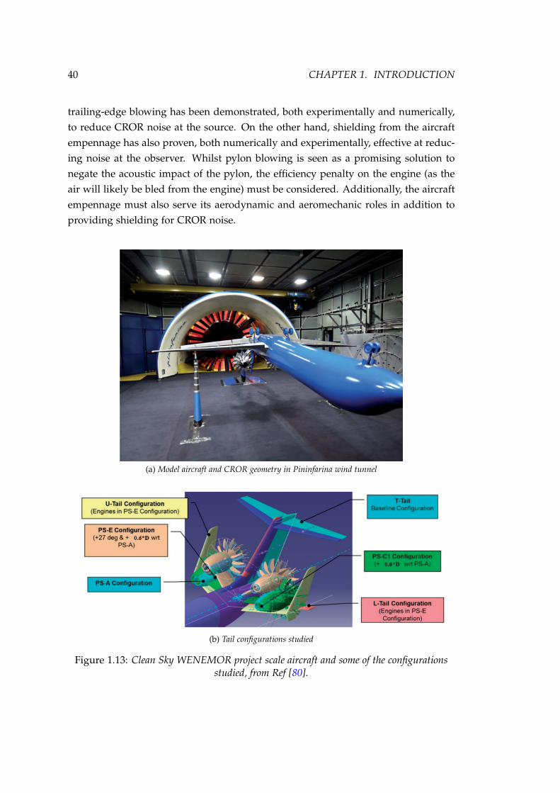
In the frame of the Clean Sky WENEMOR project [79], extensive numerical andexperimental investigations were carried out investigating installation effects of mod-ern CROR. The project tested a large number of CROR configurations and aircraftconfigurations, including U-, L- and T-tail configurations, the angle of the CRORmounting pylon and engine-wing distance, to name but a few. Figure 1.13 illustratesthe experimental facilities and the range of installation configurations consideredwithin the project.
Sanders et al. [77] detailed some of the numerical contributions to the WENEMORproject, whilst Kennedy, Eret & Bennet [80] reported on some of the experimentalwork within the project. In both experimental and numerical studies, the L- and U-tail configurations (i.e. where there is a horizontal surface below the CROR) generallyresulted in greater reductions in ground noise. Furthermore, the angled tailplaneoffered more significant noise reductions than the horizontal counterpart. However,due to the different shielding behaviours of the alone- and interaction-tones, no singleconfiguration offered noise reductions across all frequencies.
Durrwachter, Keßler & Kramer [81] presented a numerical tool-chain for assessingthe installation effects of a CROR. Using uRANS CFD data to inform an acousticsolver coupled to a BEM to compute the acoustic shielding of aircraft surfaces, theauthors investigated a number of aircraft configurations, namely T-, U- and L-tail.The authors used the EPNL metric, computed from simulated certification flyoverpoints, to compare each configuration. Therefore, the results can be more realisticallyused to gauge the relative benefit of each case. The shielding in the lateral directionshowed marginal benefits due to the symmetry of the configuration (i.e. two CROReither side of the tail-plane). In the flyover case, the L- and U-tail configurationsshowed the most significant reduction in noise.
Modern CROR are typically proposed to be pylon mounted to the airframe. How-ever, the presence of the pylon upstream of the fore rotor results in an unsteady inflowand hence a further unsteady noise source occurring at harmonics of fore BPF. Pylon
40 CHAPTER 1. INTRODUCTION
trailing-edge blowing has been demonstrated, both experimentally and numerically,to reduce CROR noise at the source. On the other hand, shielding from the aircraftempennage has also proven, both numerically and experimentally, effective at reduc-ing noise at the observer. Whilst pylon blowing is seen as a promising solution tonegate the acoustic impact of the pylon, the efficiency penalty on the engine (as theair will likely be bled from the engine) must be considered. Additionally, the aircraftempennage must also serve its aerodynamic and aeromechanic roles in addition toproviding shielding for CROR noise.
(a) Model aircraft and CROR geometry in Pininfarina wind tunnel
(b) Tail configurations studied
Figure 1.13: Clean Sky WENEMOR project scale aircraft and some of the configurationsstudied, from Ref [80].

1.3. OBJECTIVES OF THE THESIS 41
1.2.7 Summary
A survey of the open literature has been undertaken to bring together currentCROR noise-reducing concepts and the methodologies used for their analysis. Theliterature survey has identified that targeting the interaction component offers thegreatest potential for reducing CROR noise. Novel configurations have shown theability to reduce the interaction component. Additionally, optimisation methods havealso demonstrated the ability to reduce the interaction source. However, the literaturereview has shown that the use of high-order models within optimisation tools arestill currently limited by computational resources, e.g. the use of steady models foran inherently unsteady problem and a limited design space. As a result, there ispresently scope to identify further noise-reducing concepts using a range of low- andhigh-order methodologies.
1.3 Objectives of the Thesis
The main aim of this work is to develop a low-order tool-chain for the analysis ofCROR and to use this tool, supported by high-fidelity analysis, to identify potentialnoise reductions for CROR. To this end, the work presented in the thesis comprisesthe following objectives:
1. Develop and validate a low-order, multi-disciplinary CROR design tool.
2. Demonstrate the use of the design tool to identify high-performing CROR de-signs for general aviation aircraft.
3. Use the low-order CROR design tool to investigate a number of novel configu-rations for reducing CROR noise in the terminal area.
4. Perform high-order aerodynamic analysis to investigate the noise sources ofthese novel concepts.
5. Use coupled high-order aerodynamic-aeroacoustic tools to substantiate the ca-pabilities of the novel concepts.
1.4 Thesis Structure
The thesis is divided into eight chapters and proceeds as follows:
Chapter 2 is divided into two parts, presenting the low- and high-order aerodynamicmodels used in the analyses. Validation and a sensitivity analysis is presented forboth.

42 CHAPTER 1. INTRODUCTION
Chapter 3 is divided into three parts. First, CROR aeroacoustics is described withan introduction to the main noise sources. Following this, both low- and high-orderaeroacoustic models are described with an accompanying validation and sensitivityanalysis for each.
Chapter 4 focuses on the low-order structural model. Following the development ofthe model, a sensitivity analysis is presented.
Chapter 5 presents a parametric study of CROR noise, investigating the effect ofblade count and tip speed. A design study based on optimisation is then described.
Chapter 6 investigates a number of novel noise-reducing CROR concepts using thepresented low-order design tools.
Chapter 7 further investigates the novel noise-reducing CROR concepts. However,the described high-order tools are utilised to confirm the conclusions made in theprevious chapter and provide greater insight into the noise generating mechanisms.
Chapter 8 provides the main conclusions of the work and a number of recommenda-tions for future work.

Chapter 2
Aerodynamic Modelling
Aerodynamics, in the current context of CROR, is the interaction between air (theworking fluid), and the rotor blades. By studying this interaction, it is possible toestimate the performance of the CROR. In particular, how efficient the rotor bladesconvert their supplied power (from the engine), into useful power, i.e. thrust to propelthe aircraft (multiplied by the aircraft forward speed). Furthermore, the analysis ofall other aspects of the CROR analysis, e.g. noise or structural, relies on the CRORaerodynamics.
This chapter presents two approaches to studying the aerodynamics of CROR.Firstly, a low-order approach is described, whereby Blade Element Momentum The-ory (BEMT) is extended for CROR applications. The low-order method, while limitedin the detail of physics, is suitable for preliminary design studies due to its low com-putational cost. On the other hand, using a CFD solver, a high-order approach is alsotaken. Whilst more computationally expensive, the high-order analysis allows for amore in-depth analysis of the aerodynamics of the CROR.
2.1 Low-Order Aerodynamic Modelling
Low-order models are those that provide reduced physical insight for low com-putational cost. Whilst low-order models may not be appropriate for a detailed de-sign or for understanding the underlying physics of a problem; they are sufficientfor parametric and preliminary design studies. To this end, a low-order model tocompute the aerodynamic performance of CROR has been developed. This modelaims to provide sufficient details of the performance such that changes to the CRORconfiguration may be assessed.
In this section, BEMT is extended to CROR. The theory of the model is presented,followed by a validation and sensitivity study to verify the abilities and limitationsof the given model.
43

44 CHAPTER 2. AERODYNAMIC MODELLING
2.1.1 Blade Element Momentum Theory
Blade Element Momentum Theory (BEMT) combines the simplicity of Momen-tum Theory and the ability of Blade Element Theory to represent a greater geometricdetail to give a robust and reliable solution methodology for propeller and rotoranalysis.
Momentum Theory
The momentum theory of Froude [82] and Rankine [83] has been used extensivelyfor the analysis of rotary wings, including marine and aircraft propellers, helicoptersand wind turbines. Due to its low computational cost, its simplicity and the factthat little input data is required, momentum theory has been a popular method forobtaining first-order approximations of rotary-wing performance since its initial de-velopment.
Momentum theory, also known as actuator disc theory, models the propeller/ro-tor as a planar rotating disc with surrounding stream tube, Figure 2.1. Momentumtheory assumes that there is no flux through the stream tube and that the flow isincompressible and inviscid. Despite the assumption of constant velocity throughthe disc, there exists a pressure discontinuity through the disc. This discontinuityresults in a flow acceleration with accompanying contraction of the streamtube aft ofthe disc.
Figure 2.1: Representation of propeller disc in momentum theory.
The momentum theory formulation is well documented throughout the literature(see, e.g. [84, 85]), and, therefore, its development is unwarranted here. To accountfor variable inflow and wake rotation, the elemental form of momentum theory isused. The thrust and torque produced over a differential area, dA, of the disc aregiven by:
dT = 2ρ(V∞ + νix)νix dA, (2.1)

2.1. LOW-ORDER AERODYNAMIC MODELLING 45
anddQ = ρrνiθ
(V∞ + νix) dA. (2.2)
Where νix and νiθare the self induced axial and tangential velocities respectively. The
elemental area, dA, is given by∗:
dA = r dr dψ. (2.3)
Considering axisymmetric loading and using the annular formulation where dA =
2πrdr the thrust and torque are:
dT = 4πρr(V∞ + νix)νix dr, (2.4)
dQ = 2πρr2νiθ(V∞ + νix) dr. (2.5)
Blade Element Theory
Figure 2.2: Velocity and force components acting on a blade element.
Blade Element Theory (BET) is based on the discretisation of the rotor blade intoa number of discrete radial elements. The two-dimensional sectional aerodynamicsof each section is computed in isolation and are then integrated along the span togive the total rotor loads. BET requires more input data and can, therefore, providegreater detail than momentum theory for negligible additional computational cost.
Considering the velocity components at the blade element, Figure 2.2, the thrustand torque at each element are given by:
dT =12
FT NρVrel2Cacdr, (2.6)
∗The total area would be given by: A =∫ 2π
0
∫ Rrh
r dr dψ.

46 CHAPTER 2. AERODYNAMIC MODELLING
dQ =12
FT NρVrel2Cncrdr. (2.7)
Where Vrel is the relative velocity component to the blade element and from Fig-ure 2.2, is given by:
Vrel =
√Vx
2 + Vθ2 =
√(V∞ + νix)
2 + (Ωr− νiθ)2. (2.8)
The axial and normal force coefficient, Ca and Cn, are related to the local 2D aerody-namic coefficients by: [
Ca
Cn
]=
[cosφ −sinφ
sinφ cosφ
][cl
cd
]. (2.9)
The aerodynamic coefficients, cl and cd are approximated from simple aerodynamicmodels for rotary wings [86] or taken from look-up tables for a given aerofoil sectionand angle of attack. The local angle of attack is related to the inflow angle and thelocal setting angle:
α = β− φ, (2.10)
with the inflow angle φ:
φ = tan−1(
Vx
Vθ
)= tan−1
(V∞ + νix
Ωr− νiθ
). (2.11)
Finally, FT is the Prandtl correction factor [87, 88] (though Glauert’s modified versionof the tip correction is more commonly used [89]). This correction accounts for thezero loading at the blade hub and tip due to 3D effects. This simple correction iscomputed from the local blade radius and inflow angle:
fh =N (r− rh)
2r sinφ,
Fh =2cos−1 (e− fh
)π
,
ft =N (R− r)
2r sinφ,
Ft =2cos−1 (e− ft
)π
,
FT = FhFt.
(2.12)
Combined Blade Element Momentum Theory
Both momentum and blade element theories are combined to give a unified set ofequations that provide a robust and reliable numerical scheme for computing rotorperformance. From an initial guess of the induced velocities, BET is used to compute

2.1. LOW-ORDER AERODYNAMIC MODELLING 47
the initial rotor performance. Combining the momentum and blade element theoryequations, and recasting in terms of the induced velocities:
νix =dT|BET
4πρr(V∞ + νix), (2.13)
νiθ=
dQ|BET
2πρr2(V∞ + νix), (2.14)
an iterative solution methodology can be used to obtain the induced velocities andthe blade loading.
2.1.2 Extension to Counter Rotating Open Rotors
The analysis of CROR presents a complex problem. Due to the mutual interactionbetween both blade rows, in its current form, the BEMT is unsuitable to performanalysis of CROR. Therefore, to account for the interaction between blade rows, bothmomentum and blade element theories have been extended.
Momentum Theory
The extension of momentum theory to the CROR case requires the considerationof a number of additional velocity components. In addition to the self-induced com-ponents, there now exists ‘mutually-induced’ components. These mutually-inducedcomponents are introduced to account for the interaction each rotor has on the other.To proceed, Figure 2.3 shows a schematic of the updated momentum theory problem.
g
D1
D2
g/2
1
2
3
5
4
g/2
x
z
Figure 2.3: Momentum theory schematic for CROR.
The velocity components at each location in the domain comprise both self- andmutually-induced components. Mutually induced components are the product of the

48 CHAPTER 2. AERODYNAMIC MODELLING
self-induced component and an ‘interference’ coefficient. Thus, for each rotor:
νmix1 = κx21 νix2 ;
νmix2 = κx12 νix1 ;
νmiθ1 = κθ21 νiθ2 ;
νmiθ2 = κθ12 νiθ1 .
(2.15)
Where, e.g. νmix1 characterises the effect of the axial velocity of the aft rotor acting onthe fore rotor. With analogous definitions for the other terms.
The interference coefficients characterise the propagation of the self-induced termsin the direction of the opposing rotor. Beaumier [90] gives the following descriptionand values of these interference coefficients:
• κx12 ∈ [1 : 2]; the induced velocity approaches two far downstream and is equalto one at the rotor disc;
• κx21 ∈ [0 : 1]; the induced velocity is zero far upstream and equal to one at thedisc;
• κθ12 ≈ 2; the induced swirl quickly approaches 2 behind the disc;
• κθ21 ≈ 0; the swirl from the aft rotor does not propagate upstream.
To characterise the effect of spacing between the two blade rows, the following inter-ference coefficients are introduced:
κx12 =( x
D+ 1)
,
κx21 =(
1− xD
),
κθ12 =
(( xD
)1/4+ 1)
,
κθ21 = 0,
(2.16)
where x is the axial location of interest, e.g. for the velocity component at location3, this would take a value of g/2, with g the spacing between blade rows. Theseterms have been developed from results from classical momentum theory and thedescription given by Beaumier. From the interference coefficients, the velocity com-ponents at each location in the domain, Figure 2.3, can be computed, as summarisedin Table 2.1. Note that the far downstream position has been assumed to correspondto one diameter downstream (From classical momentum theory, this is the locationwhere the induced velocity is approximately twice that at the disc [91]).

2.1. LOW-ORDER AERODYNAMIC MODELLING 49
Table 2.1: CROR velocity components.
Component Axial (U) Tangential (V)1 V∞ 02 V∞ + νix1
+ νix2κx21(g) νiθ1
− νiθ2κθ21(g)
3 V∞ + νix1κx12
( g2
)+ νix2
κx21
( g2
)νiθ1
κθ12
( g2
)− νiθ2
κθ21
( g2
)4 V∞ + νix1
κx12(g) + νix2νiθ1
κθ21(g)− νiθ2
5 V∞ + νix1κx12(2R) + νix2
κx21(2R) νiθ1κθ12(2R)− νiθ2
κθ21(2R)
From the velocity components, the thrust and torque from each rotor can be com-puted. The total thrust is given by the change in axial momentum within the stream-tube. Hence,
T = m (U5 −U1) (2.17)
The total thrust is also given by the sum of the thrust from each rotor:
T = T1 + T2, (2.18)
The individual components can be approximated as:
T1 = m1(U3 −U1), (2.19)
andT2 = m2(U5 −U3). (2.20)
However, as U3 does not represent the far downstream and far upstream locationsfor the fore and aft rotors respectively, the above equations are not strictly true. Nev-ertheless, these expressions are required in order to approximate the contributionsfrom each rotor. Note that the expression for the total thrust remains true.
The thrust from each rotor can also be computed by considering the pressurejump over rotor, T = A∆p. This requires a similar assumption that the pressure inthe midplane between the rotors is equal to the ambient value. Again, whilst this isnot an accurate representation it is sufficient for approximating the individual rotorcontributions.
Returning to the momentum theory derivation and expanding the velocity termsfor the fore rotor and considering the thrust of an annular element:
dT1 =(
V∞ + νix1κx12
( g2
)+ νix2
κx21
( g2
)−V∞
)dm1. (2.21)

50 CHAPTER 2. AERODYNAMIC MODELLING
The mass flow rate through the fore rotor is expressed as:
dm1 = ρU1dA1
= 2πρr1
(V∞ + νix1
+ νix2κx21(g)
)dr1.
(2.22)
Hence, the elemental thrust produced by the fore rotor is expressed as:
dT1 = 2πρr1
(V∞ + νix1
+ νix2κx21(g)
)(νix1
κx12
( g2
)+ νix2
κx21
( g2
))dr1. (2.23)
Similarly, expanding the velocity terms for the aft rotor:
dT2 =[(
V∞ + νix1κx12(2R) + νix2
κx21(2R))−(
V∞ + νix1κx12
( g2
)+ νix2
κx21
( g2
))]dm2. (2.24)
The mass flow rate through the aft rotor is given by:
dm2 = ρU4dA2
= 2πρr2
(V∞ + νix1
κx12(g) + νix2
)dr2.
(2.25)
The elemental thrust from the aft rotor is then:
dT2 = 2πρr2
(V∞ + νix1
κx12(g) + νix2
)[νix1
(κx12(2R)− κx12
( g2
))+ νix2
(κx12(2R)− κx21
( g2
))]dr2. (2.26)
The torque produced by the CROR will be given by the change in angular mo-mentum through the streamtube. For the fore rotor, the torque is:
dQ1 = V2r1dm1. (2.27)
Substituting the mass flow rate and expanding the velocity term:
dQ1 = 2πρr12(
V∞ + νix1+ νix2
κx21(g))(
νiθ1− νiθ2
κθ21(g))
dr1. (2.28)
Similarly, for the aft rotor, the elemental torque is given by:
dQ2 = V4r2dm2. (2.29)
Again, expanding the velocity term and substituting the mass flow term:
dQ2 = 2πρr22(
V∞ + νix1κx12(g) + νix2
)(νiθ1
κθ21(g)− νiθ2
)dr2 (2.30)

2.1. LOW-ORDER AERODYNAMIC MODELLING 51
Note, the torque from each rotor will be in opposite directions and will, therefore,have a cancelling effect.
Blade Element Theory
Figure 2.4: CROR velocity triangles.
The extension of BET to application to CROR only requires that the velocity tri-angles are updated. The velocity triangles for a CROR configuration are shown inFigure 2.4. The relative velocity of each radial element then becomes:
Vrel =
√Vx
2 + Vθ2 =
√(V∞ + νix + νmix)
2 + (Ωr− νiθ+ νmiθ
)2 . (2.31)
The inflow angle is now given by:
φ = tan−1(
V∞ + νix + νmix
Ωr− νiθ+ νmiθ
). (2.32)
These are then used to compute the sectional aerodynamics and thus the thrust andtorque of each rotor using the equations above for the isolated rotor.
Combined Blade Element Momentum Theory
Similarly to the case of the isolated rotor, the momentum and blade element the-ories are combined. However, as the performance of both rotors is now stronglycoupled, a more robust solution methodology is required to solve for the rotor per-formance.
Similarly to the case of the isolated rotor, an initial guess of the induced velocities

52 CHAPTER 2. AERODYNAMIC MODELLING
is first made, i.e.:ν(0) =
(ν(0)ix1
,ν(0)ix2,ν(0)iθ1
,ν(0)iθ2
)(2.33)
The loading of each rotor is then computed using this initial guess. Following this,the blade element and momentum theory equations are combined and results in asystem of non-linear equations of the form [FFF(xxx)] = [0]:
dT1|BET − dT1|MT(νix1 ,νix2,νiθ1
,νiθ2) = 0,
dT2|BET − dT2|MT(νix1 ,νix2,νiθ1
,νiθ2) = 0,
dP1|BET − dP1|MT(νix1 ,νix2,νiθ1
,νiθ2) = 0,
dP2|BET − dP2|MT(νix1 ,νix2,νiθ1
,νiθ2) = 0.
(2.34)
To solve this system of equations, Newton’s method is used. Newton’s methodcan be easily programmed and can provide quadratic convergence (when close to thesolution). Extended to a system of non-linear equations, it is generally given by [92]:
νiνiνi(k) = νiνiνi
(k−1) − JJJ(νiνiνi(k−1))−1FFF(νiνiνi
(k−1)). (2.35)
Where FFF is a vector containing the set non-linear equations; k is the iteration counter;and JJJ is the Jacobian matrix. The Jacobian matrix is the matrix of first-order partial
derivatives, i.e.∂Fi
∂νj. In this case, the Jacobian can be solved analytically. However, in
practice, it was solved numerically using a finite differencing scheme. In particular,forward differencing was used:
(∂FFF(νννi)
∂x
)(k)
=FFF(νννi)
(k+1) − FFF(νννi)(k)
∆x+O(x) (2.36)
The use of higher-order differencing, e.g. central differences, in addition toRichardson extrapolation [93], was also investigated. However, these higher-orderapproximations showed no significant effect on the computed Jacobian or inducedvelocities. Therefore, given the additional computational cost, they were not used.
For cases where the initial guess is far from the solution, Newton’s method willconverge very slowly. For generic CROR geometries and operating point, a reason-able initial guess may not be first obvious. To overcome this, and to improve therobustness of the numerical method, the Levenberg-Marquardt algorithm [94, 95] wasimplemented to solve the BEMT system of equations.
Newton’s method is fundamentally based on the evaluation of the search direc-tion, dk, which from Equations (2.35) is JJJ(ννν(k)i )−1FFF(ννν(k)i ). The Levenberg-Marquardtalgorithm provides a more robust evaluation of the search direction, not failing when
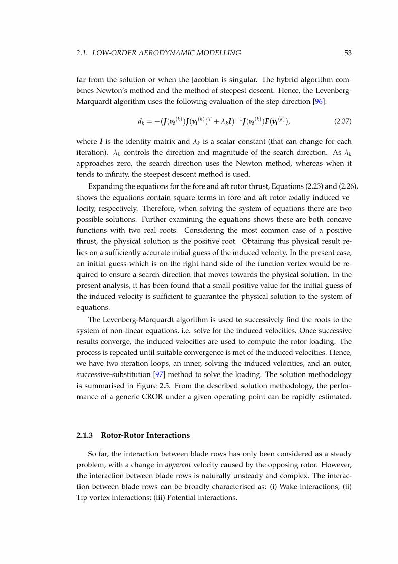
2.1. LOW-ORDER AERODYNAMIC MODELLING 53
far from the solution or when the Jacobian is singular. The hybrid algorithm com-bines Newton’s method and the method of steepest descent. Hence, the Levenberg-Marquardt algorithm uses the following evaluation of the step direction [96]:
dk = −(JJJ(νiνiνi(k))JJJ(νiνiνi
(k))T + λkIII)−1JJJ(νiνiνi(k))FFF(νiνiνi
(k)), (2.37)
where III is the identity matrix and λk is a scalar constant (that can change for eachiteration). λk controls the direction and magnitude of the search direction. As λk
approaches zero, the search direction uses the Newton method, whereas when ittends to infinity, the steepest descent method is used.
Expanding the equations for the fore and aft rotor thrust, Equations (2.23) and (2.26),shows the equations contain square terms in fore and aft rotor axially induced ve-locity, respectively. Therefore, when solving the system of equations there are twopossible solutions. Further examining the equations shows these are both concavefunctions with two real roots. Considering the most common case of a positivethrust, the physical solution is the positive root. Obtaining this physical result re-lies on a sufficiently accurate initial guess of the induced velocity. In the present case,an initial guess which is on the right hand side of the function vertex would be re-quired to ensure a search direction that moves towards the physical solution. In thepresent analysis, it has been found that a small positive value for the initial guess ofthe induced velocity is sufficient to guarantee the physical solution to the system ofequations.
The Levenberg-Marquardt algorithm is used to successively find the roots to thesystem of non-linear equations, i.e. solve for the induced velocities. Once successiveresults converge, the induced velocities are used to compute the rotor loading. Theprocess is repeated until suitable convergence is met of the induced velocities. Hence,we have two iteration loops, an inner, solving the induced velocities, and an outer,successive-substitution [97] method to solve the loading. The solution methodologyis summarised in Figure 2.5. From the described solution methodology, the perfor-mance of a generic CROR under a given operating point can be rapidly estimated.
2.1.3 Rotor-Rotor Interactions
So far, the interaction between blade rows has only been considered as a steadyproblem, with a change in apparent velocity caused by the opposing rotor. However,the interaction between blade rows is naturally unsteady and complex. The interac-tion between blade rows can be broadly characterised as: (i) Wake interactions; (ii)Tip vortex interactions; (iii) Potential interactions.
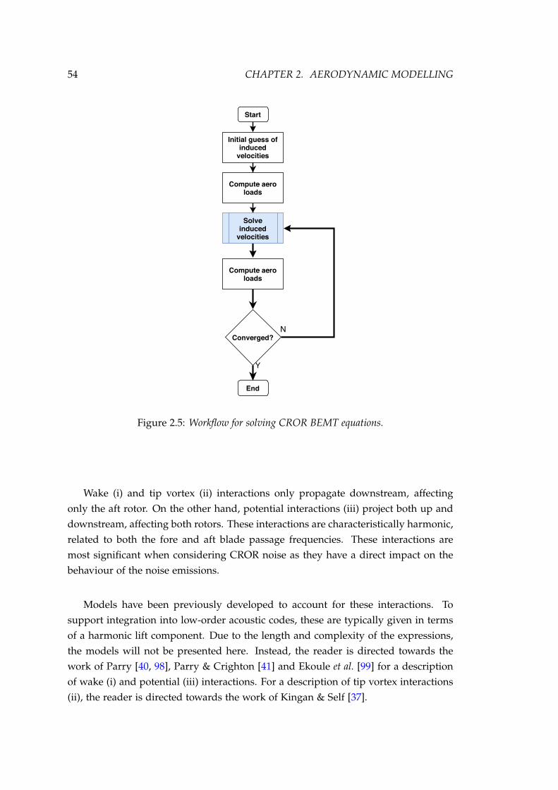
54 CHAPTER 2. AERODYNAMIC MODELLING
Start
Initial guess ofinduced
velocities
Compute aeroloads
Compute aeroloads
End
Converged?
Solveinduced
velocities
Y
N
Figure 2.5: Workflow for solving CROR BEMT equations.
Wake (i) and tip vortex (ii) interactions only propagate downstream, affectingonly the aft rotor. On the other hand, potential interactions (iii) project both up anddownstream, affecting both rotors. These interactions are characteristically harmonic,related to both the fore and aft blade passage frequencies. These interactions aremost significant when considering CROR noise as they have a direct impact on thebehaviour of the noise emissions.
Models have been previously developed to account for these interactions. Tosupport integration into low-order acoustic codes, these are typically given in termsof a harmonic lift component. Due to the length and complexity of the expressions,the models will not be presented here. Instead, the reader is directed towards thework of Parry [40, 98], Parry & Crighton [41] and Ekoule et al. [99] for a descriptionof wake (i) and potential (iii) interactions. For a description of tip vortex interactions(ii), the reader is directed towards the work of Kingan & Self [37].

2.1. LOW-ORDER AERODYNAMIC MODELLING 55
2.1.4 2D Aerodynamics
To compute the total rotor loads, the BEMT method relies on the aerodynamicproperties of each radial element along the span. The aerodynamic properties mustbe known for a range of angles of attack for each aerofoil at each radial element.
In the present work, the aerodynamic data comes from a number of sources. Forexample, a look-up table has been generated for the NACA-65 aerofoil family fromthe experimental data of Abbot & von Doenhoff [100]. Collation of the experimentaldata results in a database of aerodynamic properties for NACA-65 aerofoils account-ing for thickness, camber and angle of attack. A database for the NACA-16 familywas also constructed, however, using a 2D aerofoil code. The aerodynamic propertiesat each radial element are then interpolated from the look-up table.
The small changes in thickness and camber, combined with the changes in theangle of attack along the span, when interpolated from the look-up tables, typicallyresults in a non-continuous distribution along the span. This discontinuity tends tomake the convergence of the BEMT more difficult. However, this difficulty may beovercome by smoothing the solution along the span.
Another data source is to use some aerodynamic approximations to the aerofoilbehaviour. From thin aerofoil theory, the lift coefficient is approximated. The drag co-efficient, on the other hand, is computed from the method presented by Bailey [101]for calculating the aerodynamics of a lifting rotor. Whilst this data has a greaternumber of assumptions about the flow, it does not suffer the same numerical prob-lems of the look-up tables. Furthermore, they are less computationally expensive. Aswill be demonstrated later, these approximations also provide sufficient accuracy inpredicting the rotor performance.
2.1.5 Model Corrections
To improve the capabilities and minimise the limitations of the CROR aerody-namic analysis, a number of corrections can be added. For example, the Karmen-Tsien compressibility correction and a drag divergence model [102] can be usedto account for the effects of higher Mach numbers. Modern civil aviation CRORtypically feature high blade count designs; therefore, a cascade correction can beused to account for the interaction that will occur between blades towards the bladeroot [103]. The Prandtl tip correction was used included to account for 3D effects.The simple model presented by Stepniewski & Keys [104] was used to compute theradius of contraction to account for the effects of streamtube contraction. Outsidethis radius, no effects of mutual interaction were accounted for. The aerofoil data,both approximations and look-up tables are appropriate only in a range of anglesof attack. Leishmann [105] suggest a sinusoidal profile to lift and drag coefficients

56 CHAPTER 2. AERODYNAMIC MODELLING
to extend the 2D aerodynamics to ±180, thus extending the range of the aerofoildatabase.
2.1.6 Rotor Trim
The analysis of rotor blades typically requires the matching of thrust or torque tocompare rotor performance. Similarly, the operation of rotor blades requires a giventhrust or torque to be delivered to meet the aircraft requirements. The rotor blade canbe trimmed to provide the required thrust by either varying the blade setting angleor the rotor rotational speed. Figure 2.6 defines the setting angles and direction ofrotation of each rotor used in the analysis.
Figure 2.6: Definition of CROR fore and aft rotor setting angles and rotation senses.
To trim the rotor blades, either the blade setting angle or rotor rotational speedwas successively altered until the thrust or torque produced was within a given tol-erance of the required value. To aid convergence to the required value, the change insetting angle or rotor rotational speed was computed according to:
∆ = ∆ + γ+|ζ − ζT|, ζ < ζT
∆ = ∆− γ−|ζ − ζT|, ζ > ζT(2.38)
∆ represents either blade setting angle (β) or rotor speed (Ω); ζ is the computedthrust or torque, and ζT the corresponding required value; γ+ and γ− are numer-ical gains. For trimming by setting angle, these gains are of the order 10−5, whilstwhen trimming by rotational speed, these are of the order 10−2. To avoid a solutionoscillating about a given value, it is recommended to have different values of γ+ andγ−.
The CROR trimming procedure comprises two iterative loops. The first loopadjusts either rotational speed or setting angle of the the aft rotor (depending on

2.1. LOW-ORDER AERODYNAMIC MODELLING 57
input specification). Once the aft rotor has met the trim requirements, the seconditerative loop adjust the fore rotor. After each adjustment of fore rotor rotationalspeed or setting angle, the aft rotor trim is then re-evaluated. The procedure isdemonstrated in Figure 2.7. The procedure implemented only allows for adjustmentsin either setting angle or rotational speed. Whilst one is varied, the other is heldconstant. This avoids issues surrounding multiple solutions to the trim variable.
Start
Compute Aero
Loads
Aft rotor trimmed?
Fore rotor trimmed?
End
Adjust aftsetting angle
or rotational speed
Adjust foresetting angle
or rotational speed
Y
Y
N
N
Figure 2.7: Implemented rotor trimming routine.
2.1.7 Model Validation
To verify the BEMT predictions, the CROR aerodynamic model has been com-pared against a number of available experimental and numerical data. Whilst CRORdata is scarce, a number of performance data have been obtained to perform thevalidation. These data sets cover a range of configurations and operating points.
SR2 CROR
The BEMT model is first compared against the experimental work presented byDunham et al. [106]. Both flowfield and thrust coefficient data were obtained for a

58 CHAPTER 2. AERODYNAMIC MODELLING
0.409 m diameter CROR of SR2 design [107]. The SR2 is a straight-bladed propellerfrom the NASA Advanced Turboprop Project [7], used as a baseline for investigationsinto the effect of sweep. The spanwise geometry of the SR2 propeller is presented inFigure 2.8.
r/R
c/D
[-]
t/c
[-]
Tw
ist
[ra
d]
Cld
[-]
0.2 0.4 0.6 0.8 1
0.06
0.08
0.1
0.12
0.14
0.16
0
0.02
0.04
0.06
0.08
0.1
0.12
0.14
0.16
0.18
0.6
0.7
0.8
0.9
1
1.1
1.2
-0.2
-0.15
-0.1
-0.05
0
0.05
0.1
0.15
0.2c/D
t/c
Twist
Cld
Figure 2.8: SR2 spanwise geometry.
Figure 2.9 compares the thrust coefficient computed using the BEMT model andthe experimental data obtained by Dunham et al. [106] for 4 × 4 and 8 × 8 CRORconfigurations. Results are compared over a range of advance ratios at a fore and aftblade setting angle of β.75 = 40.3.
Advance Ratio, J []
Th
rus
t C
oe
ffic
ien
t, C
T [
]
0.8 1 1.2 1.4 1.6 1.8
0.2
0.4
0.6
0.8
1
1.2
1.4
N1 = N
2 = 4
N1 = N
2 = 8
BEMTEXP
Figure 2.9: Comparison of SR2 thrust coefficient.
Figure 2.9 shows that for both configurations, the thrust coefficient is generallywell predicted. For the 8× 8 configuration, the thrust coefficient is predicted wellover the entire range of advance ratios. On the other hand, for the 4× 4 configuration,

2.1. LOW-ORDER AERODYNAMIC MODELLING 59
the thrust coefficient is predicted well for J ≤ 1.4; beyond this, there is a significantdiscrepancy between the reported and computed data. This region of advance ratioresults in a reduced angle of attack. At the extremes, this results in a negative angle ofattack at some areas along the span. The discrepancy, therefore, may result from thepoor aerodynamic resolution at low angles of attack. However, as the data presentedby Dunham et al. did not include an analysis of errors, it is difficult to isolate thesources of the discrepancy.
The flowfield of a 4 × 4 CROR operating at an advance ratio of J = 1.21 wascomputed by Dunham et al. using laser velocimetry. The rotational speed of bothrotors were assumed equal and their value computed from an assumed free-streamvelocity (within a reported range of speeds). Three components of velocity weretaken at a number of axial planes, Figure 2.10, and averaged over a minute.
(a) Location of velocimetry recording points (b) Velocity components
Figure 2.10: Location of probes and CROR reference frame.
Figures 2.11 and 2.12 compare the axial and tangential velocity components fromthe BEMT method and those reported by Dunham et al. The BEMT model neglectsthe radial flow and is, therefore, not compared with the published data. Figure 2.11shows that the BEMT model has generally predicted the axial velocity profile wellas it travels downstream. Whilst the downstream aft rotor location is generally wellpredicted, the upstream, downstream fore rotor and far downstream locations showa discrepancy with the experimental data. The maximum discrepancy between theBEMT model and experimental data was found at the far downstream location andcorresponded to ∼ 10%. Given the agreement with experimental data for the thrustcoefficient at the current advance ratio, a better agreement would be expected forthe flowfield. Therefore, the observed discrepancy may be due to the combination
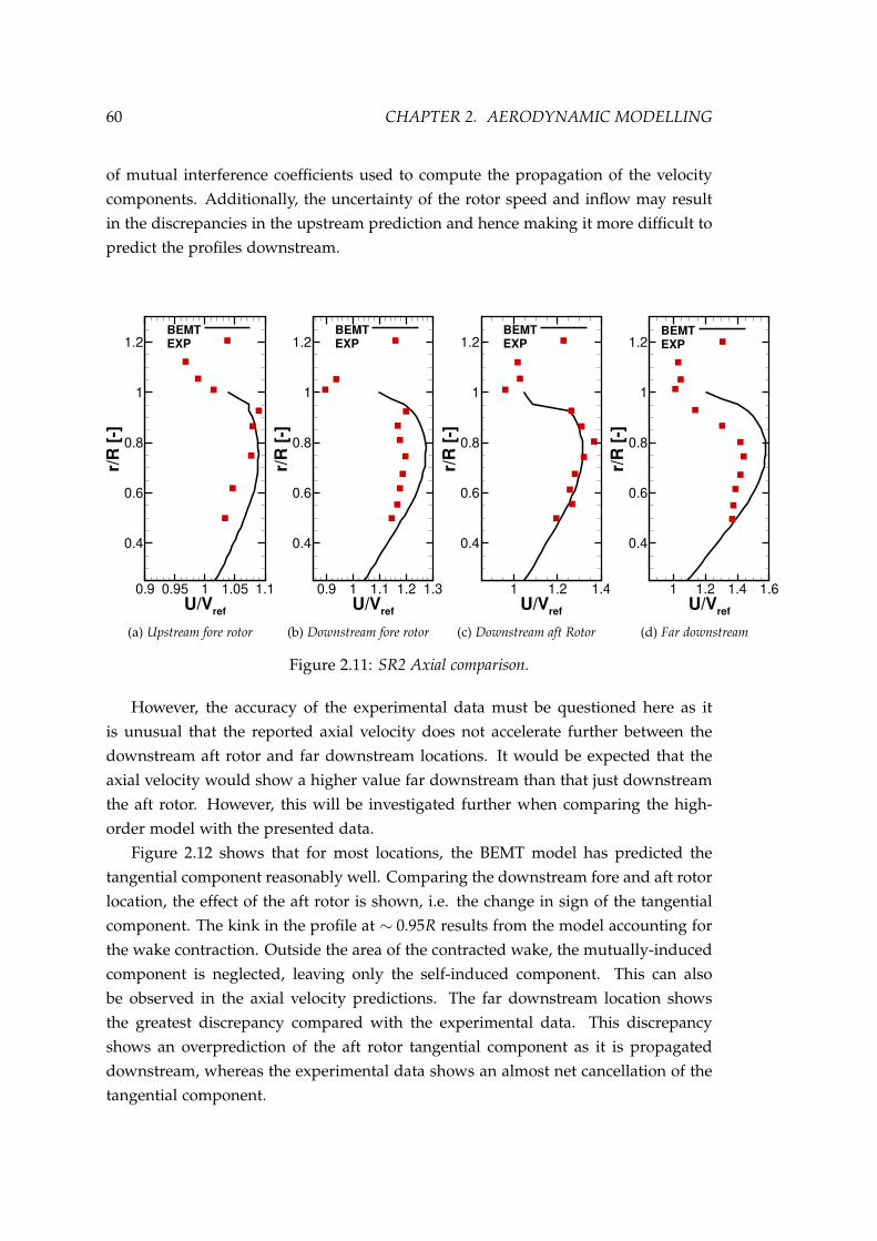
60 CHAPTER 2. AERODYNAMIC MODELLING
of mutual interference coefficients used to compute the propagation of the velocitycomponents. Additionally, the uncertainty of the rotor speed and inflow may resultin the discrepancies in the upstream prediction and hence making it more difficult topredict the profiles downstream.
U/Vref
r/R
[]
0.9 0.95 1 1.05 1.1
0.4
0.6
0.8
1
1.2
BEMTEXP
(a) Upstream fore rotor
U/Vref
r/R
[]
0.9 1 1.1 1.2 1.3
0.4
0.6
0.8
1
1.2
BEMTEXP
(b) Downstream fore rotor
U/Vref
r/R
[]
1 1.2 1.4
0.4
0.6
0.8
1
1.2
BEMTEXP
(c) Downstream aft Rotor
U/Vref
r/R
[]
1 1.2 1.4 1.6
0.4
0.6
0.8
1
1.2BEMTEXP
(d) Far downstream
Figure 2.11: SR2 Axial comparison.
However, the accuracy of the experimental data must be questioned here as itis unusual that the reported axial velocity does not accelerate further between thedownstream aft rotor and far downstream locations. It would be expected that theaxial velocity would show a higher value far downstream than that just downstreamthe aft rotor. However, this will be investigated further when comparing the high-order model with the presented data.
Figure 2.12 shows that for most locations, the BEMT model has predicted thetangential component reasonably well. Comparing the downstream fore and aft rotorlocation, the effect of the aft rotor is shown, i.e. the change in sign of the tangentialcomponent. The kink in the profile at ∼ 0.95R results from the model accounting forthe wake contraction. Outside the area of the contracted wake, the mutually-inducedcomponent is neglected, leaving only the self-induced component. This can alsobe observed in the axial velocity predictions. The far downstream location showsthe greatest discrepancy compared with the experimental data. This discrepancyshows an overprediction of the aft rotor tangential component as it is propagateddownstream, whereas the experimental data shows an almost net cancellation of thetangential component.
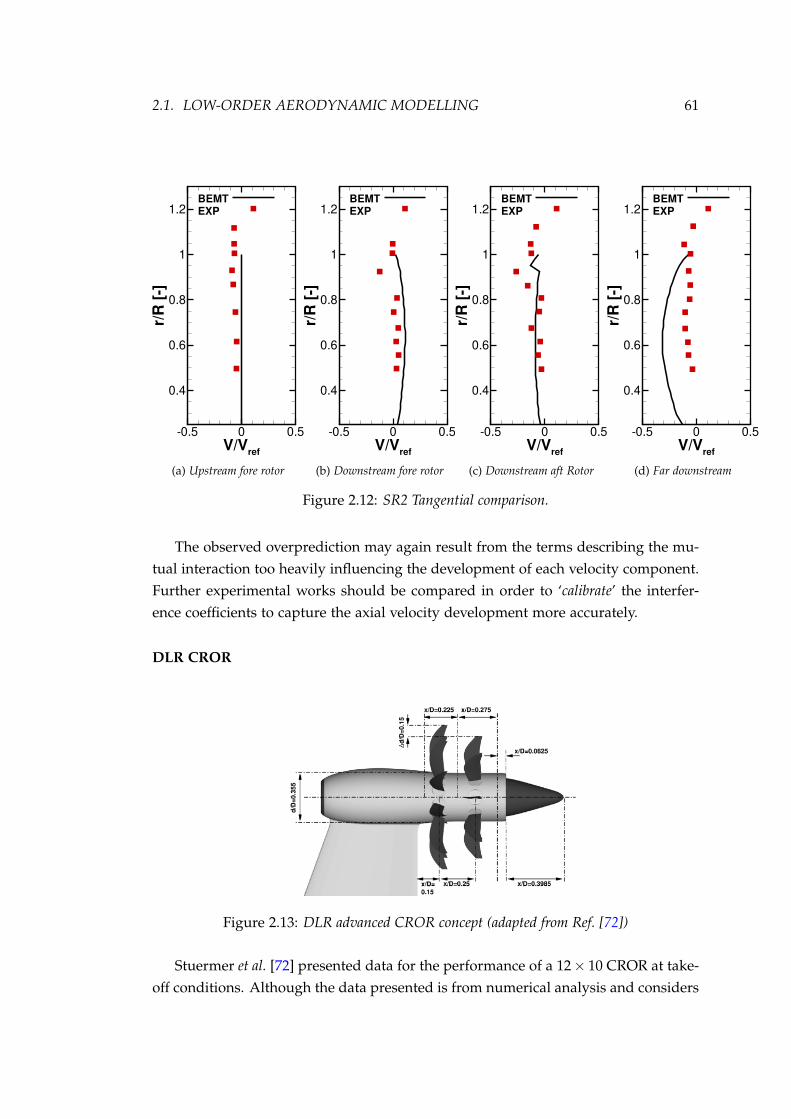
2.1. LOW-ORDER AERODYNAMIC MODELLING 61
V/Vref
r/R
[]
0.5 0 0.5
0.4
0.6
0.8
1
1.2BEMTEXP
(a) Upstream fore rotor
V/Vref
r/R
[]
0.5 0 0.5
0.4
0.6
0.8
1
1.2BEMTEXP
(b) Downstream fore rotor
V/Vref
r/R
[]
0.5 0 0.5
0.4
0.6
0.8
1
1.2BEMTEXP
(c) Downstream aft Rotor
V/Vref
r/R
[]
0.5 0 0.5
0.4
0.6
0.8
1
1.2BEMTEXP
(d) Far downstream
Figure 2.12: SR2 Tangential comparison.
The observed overprediction may again result from the terms describing the mu-tual interaction too heavily influencing the development of each velocity component.Further experimental works should be compared in order to ‘calibrate’ the interfer-ence coefficients to capture the axial velocity development more accurately.
DLR CROR
Figure 2.13: DLR advanced CROR concept (adapted from Ref. [72])
Stuermer et al. [72] presented data for the performance of a 12× 10 CROR at take-off conditions. Although the data presented is from numerical analysis and considers

62 CHAPTER 2. AERODYNAMIC MODELLING
only a single point, it useful to test the model against as it represents a modern andadvanced CROR design. Figure 2.13 shows the CROR configurations studied byStuermer et al. The data presented is also useful as it presents individual blade loadsin addition to setting angles. To compare the results, the BEMT model was trimmedto match the reported thrust coefficient with both rotors rotating at the reported 1100rev/min.
Table 2.2 compares the computed loading coefficients and blade setting anglescalculated using the BEMT model and the DLR-TAU CFD solver. Table 2.2 illustratesthat when trimmed to the same thrust coefficient, the BEMT model is able to predictrelatively well fore and aft power coefficients. The BEMT model is shown to matchwell the corresponding setting angle required to trim the rotor.
The aft rotor shows an ∼ 4% disagreement in resulting power coefficient. This dis-agreement may arise due to an overprediction of the mutually induced component.An increased axial component will result in an increased inflow angle, requiring anincreased setting angle to deliver the same angle of attack to provide the requiredthrust. Table 2.2 also shows the increased setting angle required.
Table 2.2: DLR CROR performance computed using CFD and BEMT model.
CT1[-] CT2[-] CP1[-] CP2[-] β1.75 [] β2.75 [
]BEMT 0.3915 0.2882 0.5804 0.4835 35.08 45.62DLR 0.3915 0.2883 0.5793 0.4647 34.85 41.40∆ [%] 0 0.035 0.190 3.97 0.657 9.70
Rig-140 CROR
Zachariadis & Hall [108] presented both numerical and experimental data for theRolls-Royce Rig-140 CROR. Rolls-Royce developed the Rig-140 CROR for investiga-tions into the viability of CROR in the 1980s. This case is considered highly usefulas the CROR has a number of design features of modern CROR whilst also havingexperimental data available to compare with. Rig-140 is shown in Figure 2.14.
The Rig-140 model is a 7 × 7 CROR with straight blades. Whilst the detailedblade geometry remains proprietary, Zachariadis and Hall provided sufficient detail,Figure 2.14, to compare with the BEMT model. Whilst the detail is sufficient forBEMT analysis, there is insufficient detail to compare using high-order methods.
As reported by Zachariadis & Hall [108], thrust and power coefficient changesresulted from changes in the rotational speed at a constant setting angle. Therefore,this was replicated in order to compare the BEMT model. The range of advance ratiosand hence rotor speeds were worked back from the combination of thrust and power

2.1. LOW-ORDER AERODYNAMIC MODELLING 63
(a) Rig-140 (b) Rig-140 spanwise geometry
Figure 2.14: Details of the Rolls-Royce Rig-140 CROR (adapted from Ref. [108]).
coefficient and power coefficient and efficiency plots, i.e. from the expression: η =
JCT/CP. Whilst this does not necessarily replicate the test conditions, in particularunequal rotor speeds, it is acceptable here in order to make a comparison given thelack of available data.
Figure 2.15 compares the total thrust and power coefficients for the range of ad-vance ratios computed using the BEMT model and the CFD and experimental resultsreported by Zachariadis & Hall at cruise conditions.
The BEMT model is seen to compare very well with both experimental and CFDresults up to ∼ CP = 3, beyond this range, the BEMT diverges from the experimentalresults but agrees well with the CFD results up to ∼ CP = 4. The source of dis-agreement is not immediately apparent as thrust and power results are not isolated.Isolating the disagreement is further complicated by the likely difference in rotorspeeds. The disagreement between CFD and experimental data is reported to bewith deflections of the physical blades under operation not captured using CFD.These deflections are also not captured in the BEMT model and likely one of the rea-sons for the disagreement. Furthermore, no analysis of the experimental errors wasreported, making it yet more difficult to identify the sources of error with the BEMTmodel.
2.1.8 Sensitivity Analysis
To validate the predictions of the BEMT model, it has been compared against anumber of numerical and experimental data sets. The validation showed that while
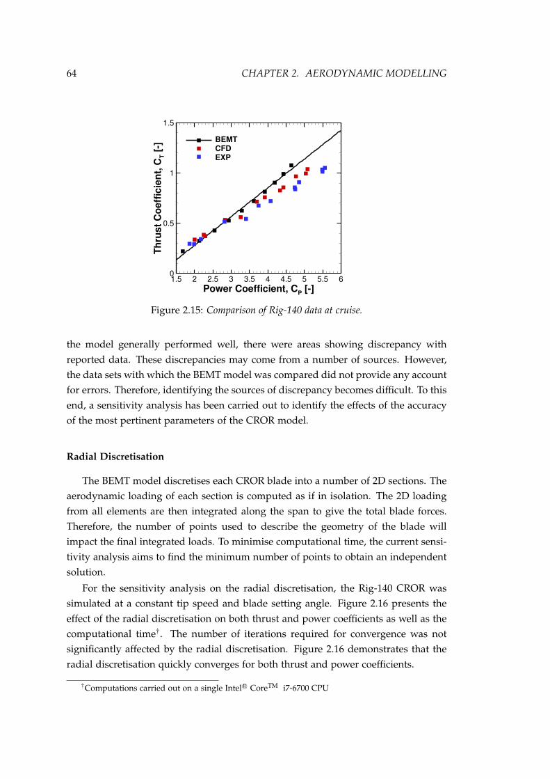
64 CHAPTER 2. AERODYNAMIC MODELLING
Power Coefficient, CP []
Th
rus
t C
oe
ffic
ien
t, C
T [
]
1.5 2 2.5 3 3.5 4 4.5 5 5.5 60
0.5
1
1.5
BEMTCFDEXP
Figure 2.15: Comparison of Rig-140 data at cruise.
the model generally performed well, there were areas showing discrepancy withreported data. These discrepancies may come from a number of sources. However,the data sets with which the BEMT model was compared did not provide any accountfor errors. Therefore, identifying the sources of discrepancy becomes difficult. To thisend, a sensitivity analysis has been carried out to identify the effects of the accuracyof the most pertinent parameters of the CROR model.
Radial Discretisation
The BEMT model discretises each CROR blade into a number of 2D sections. Theaerodynamic loading of each section is computed as if in isolation. The 2D loadingfrom all elements are then integrated along the span to give the total blade forces.Therefore, the number of points used to describe the geometry of the blade willimpact the final integrated loads. To minimise computational time, the current sensi-tivity analysis aims to find the minimum number of points to obtain an independentsolution.
For the sensitivity analysis on the radial discretisation, the Rig-140 CROR wassimulated at a constant tip speed and blade setting angle. Figure 2.16 presents theeffect of the radial discretisation on both thrust and power coefficients as well as thecomputational time†. The number of iterations required for convergence was notsignificantly affected by the radial discretisation. Figure 2.16 demonstrates that theradial discretisation quickly converges for both thrust and power coefficients.
†Computations carried out on a single Intel R© CoreTM i7-6700 CPU
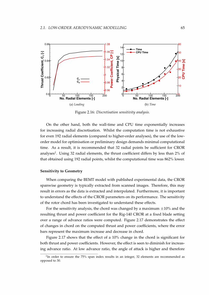
2.1. LOW-ORDER AERODYNAMIC MODELLING 65
No. Radial Elements []
Th
rus
t C
oe
ffic
ien
t, C
T [
]
Po
we
r C
oe
ffic
ien
t, C
P [
]
0 50 100 150 2000.6
0.62
0.64
0.66
0.96
0.98
1
1.02
1.04
1.06
1.08
CT
CP
(a) Loading
No. Radial Elements []
Ph
ys
ica
l T
ime
[s
]
CP
U T
ime
[s
]
0 50 100 150 2000
2
4
6
8
10
12
14
0
10
20
30
40
50
60
TimeCPU Time
(b) Time
Figure 2.16: Discretisation sensitivity analysis.
On the other hand, both the wall-time and CPU time exponentially increasesfor increasing radial discretisation. Whilst the computation time is not exhaustivefor even 192 radial elements (compared to higher-order analyses), the use of the low-order model for optimisation or preliminary design demands minimal computationaltime. As a result, it is recommended that 32 radial points be sufficient for CRORanalyses‡. Using 32 radial elements, the thrust coefficient differs by less than 2% ofthat obtained using 192 radial points, whilst the computational time was 862% lower.
Sensitivity to Geometry
When comparing the BEMT model with published experimental data, the CRORspanwise geometry is typically extracted from scanned images. Therefore, this mayresult in errors as the data is extracted and interpolated. Furthermore, it is importantto understand the effects of the CROR parameters on its performance. The sensitivityof the rotor chord has been investigated to understand these effects.
For the sensitivity analysis, the chord was changed by a maximum ±10% and theresulting thrust and power coefficient for the Rig-140 CROR at a fixed blade settingover a range of advance ratios were computed. Figure 2.17 demonstrates the effectof changes in chord on the computed thrust and power coefficients, where the errorbars represent the maximum increase and decrease in chord.
Figure 2.17 shows that the effect of a 10% change in the chord is significant forboth thrust and power coefficients. However, the effect is seen to diminish for increas-ing advance ratio. At low advance ratio, the angle of attack is higher and therefore
‡In order to ensure the 75% span index results in an integer, 32 elements are recommended asopposed to 30.

66 CHAPTER 2. AERODYNAMIC MODELLING
Advance Ratio, J []
Th
rus
t C
oe
ffic
ien
t, C
T [
]
Po
we
r C
oe
ffic
ien
t, C
P [
]
3 3.5 4 4.5 5
0.2
0.4
0.6
0.8
1
1.2
1.4
1
1.5
2
2.5
3
3.5
4
4.5
5
CT
CP
Figure 2.17: Effect of chord data on CROR performance.
more critical to design changes.
To investigate further, Figure 2.18a shows the effect of changes in the chord ata constant advance ratio. Figure 2.18a shows that the effect of chord changes areslightly more important for the power coefficient. It is also observed that both thrustand power coefficient respond linearly to the changes in the chord. This result isexpected given the blade element equations describing the loading terms. A 10%change in the chord is shown to have ∼ 5% and ∼ 6% change in thrust and powercoefficients, respectively — not insignificant. However, in terms of capturing thereported geometry, chord changes are unlikely to be this large.
∆c [%]
∆C
T,
∆C
P [%
]
10 5 0 5 10
6
4
2
0
2
4
6 CT
CP
J = 4
(a) Constant advance ratioAdvance Ratio, J []
∆C
T,
∆C
P [%
]
3.2 3.6 4 4.4 4.81.5
2
2.5
3
3.5
CT
CP
∆c = 6%
(b) Constant chord
Figure 2.18: Detailed performance effect of changes in rotor chord.

2.1. LOW-ORDER AERODYNAMIC MODELLING 67
Figure 2.18b presents the effect of a constant chord change over a range of ad-vance ratios. Figure 2.18b highlights the diminishing effect of the chord at higheradvance ratios. It is shown that the thrust coefficient diminishes much more quicklyfor increasing advance ratio.
With respect to the SR2 validation, which showed the most considerable discrep-ancy at the higher advance ratios, it is unlikely that the inaccuracies of the capturedgeometry are to blame for the disagreement.
Sensitivity to Aerodynamic Data
The CROR BEMT model requires 2D sectional aerodynamic data to compute therotor loads. The developed model can take this sectional data from either look-uptables for a given aerofoil section or from a linear approximation (§2.1.4).
Data taken from look-up tables populated with experimental data will have twoprimary sources of limitations. Firstly, the data will be for isolated aerofoils, notaccounting for 3D effects and interaction with other radial sections. Secondly, thedata is linearly interpolated from the table. The relationship with the given parametermay not be linearly dependent, and hence the interpolation will result in incorrectvalues.
For data taken from aerofoil aerodynamic codes or the linear approximations, theinherent approximations will result in inaccuracies in the resulting aerodynamics. Tothis end, a sensitivity analysis has been performed to investigate the effects of smallchanges in 2D aerodynamic data. For the study, the Rig-140 CROR was studied ata fixed setting angle over a range of advance ratios with linear aerodynamics usedto represent the sectional loads. In each case, the lift and drag coefficients wereindependently altered by ±10%.
Figure 2.19 demonstrates the effect of lift and drag coefficients on the resultingtotal CROR thrust and power coefficients over a range of advance ratios. Figure 2.19shows that, compared to the drag coefficient, the changes in the lift coefficient hasa greater impact on both thrust and power coefficients over the entire advance ratiorange. However, in both cases, their effect diminishes with increasing advance ratio.As described previously, this is due to the increased angle of attack at low advanceratios being more critical to design changes.
To investigate the effects of aerodynamic coefficients further, Figure 2.20 presentsthe change in thrust and power coefficient at a single advanced ratio for ±10% changein the aerodynamic coefficient.
Figure 2.20a shows that the effect of the lift coefficient is similar for both thrustand power coefficients. For increasing lift coefficient, both thrust and power coef-ficients linearly increase. A maximum ±5% change is observed for the maximum

68 CHAPTER 2. AERODYNAMIC MODELLING
Advance Ratio, J []
Th
rus
t C
oe
ffic
ien
t, C
T [
]
Po
we
r C
oe
ffic
ien
t, C
P [
]3.5 4 4.5
0.2
0.4
0.6
0.8
1
1.2
1.4
1
1.5
2
2.5
3
3.5
4
4.5
5
CT
CP
(a) Lift coefficientAdvance Ratio, J []
Th
rus
t C
oe
ffic
ien
t, C
T [
]
Po
we
r C
oe
ffic
ien
t, C
P [
]
3.5 4 4.50.2
0.4
0.6
0.8
1
1.2
1.4
1
1.5
2
2.5
3
3.5
4
4.5
5
CT
CP
(b) Drag coefficient
Figure 2.19: Effect of aerodynamic data on CROR performance.
∆cl [%]
∆C
T,
∆C
P [%
]
10 5 0 5 10
5
0
5
CT
CP
J = 4
(a) Lift coefficient
∆cl [%]
∆C
T,
∆C
P [%
]
10 5 0 5 102
1
0
1
2
CT
CP
J = 4
(b) Drag coefficient
Figure 2.20: Effect of aerodynamic data at constant advance ratio.
changes in lift coefficient. For the drag coefficient, Figure 2.20b shows that it has agreater effect on the thrust coefficient, with a negligible effect on the power coefficientat this advance ratio. However, the maximum change now observed is < 1% for themaximum changes in the drag coefficient.
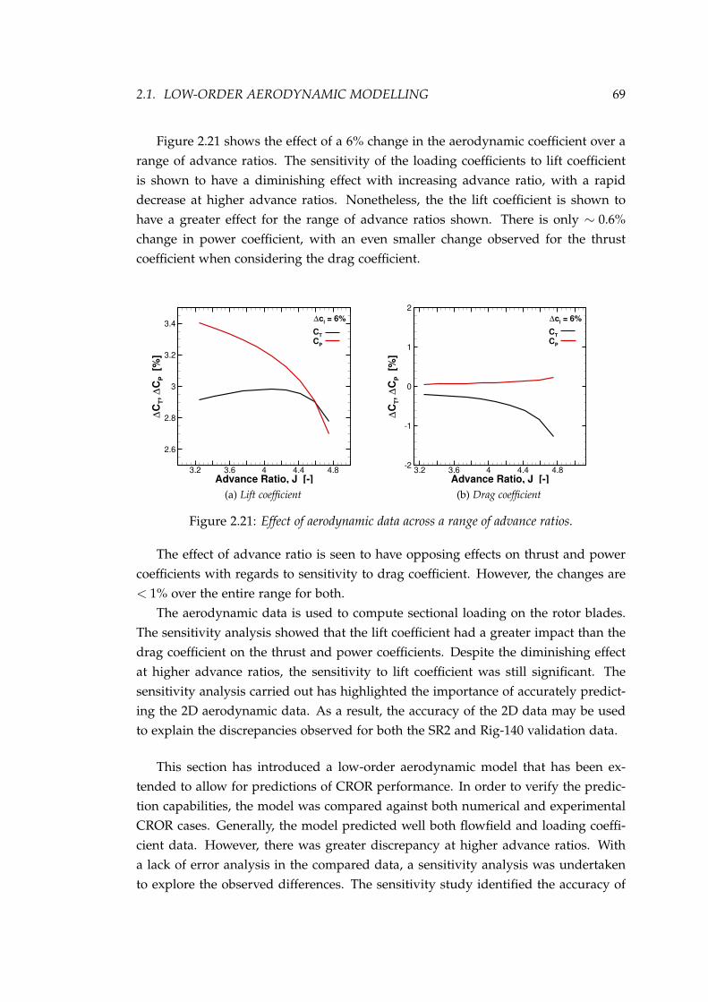
2.1. LOW-ORDER AERODYNAMIC MODELLING 69
Figure 2.21 shows the effect of a 6% change in the aerodynamic coefficient over arange of advance ratios. The sensitivity of the loading coefficients to lift coefficientis shown to have a diminishing effect with increasing advance ratio, with a rapiddecrease at higher advance ratios. Nonetheless, the the lift coefficient is shown tohave a greater effect for the range of advance ratios shown. There is only ∼ 0.6%change in power coefficient, with an even smaller change observed for the thrustcoefficient when considering the drag coefficient.
Advance Ratio, J []
∆C
T,
∆C
P [%
]
3.2 3.6 4 4.4 4.8
2.6
2.8
3
3.2
3.4
CT
CP
∆cl = 6%
(a) Lift coefficientAdvance Ratio, J []
∆C
T,
∆C
P [%
]
3.2 3.6 4 4.4 4.82
1
0
1
2
CT
CP
∆cl = 6%
(b) Drag coefficient
Figure 2.21: Effect of aerodynamic data across a range of advance ratios.
The effect of advance ratio is seen to have opposing effects on thrust and powercoefficients with regards to sensitivity to drag coefficient. However, the changes are< 1% over the entire range for both.
The aerodynamic data is used to compute sectional loading on the rotor blades.The sensitivity analysis showed that the lift coefficient had a greater impact than thedrag coefficient on the thrust and power coefficients. Despite the diminishing effectat higher advance ratios, the sensitivity to lift coefficient was still significant. Thesensitivity analysis carried out has highlighted the importance of accurately predict-ing the 2D aerodynamic data. As a result, the accuracy of the 2D data may be usedto explain the discrepancies observed for both the SR2 and Rig-140 validation data.
This section has introduced a low-order aerodynamic model that has been ex-tended to allow for predictions of CROR performance. In order to verify the predic-tion capabilities, the model was compared against both numerical and experimentalCROR cases. Generally, the model predicted well both flowfield and loading coeffi-cient data. However, there was greater discrepancy at higher advance ratios. Witha lack of error analysis in the compared data, a sensitivity analysis was undertakento explore the observed differences. The sensitivity study identified the accuracy of

70 CHAPTER 2. AERODYNAMIC MODELLING
aerodynamic data to be the most significant factor in explaining the discrepancies.
2.2 High-Order Aerodynamic Modelling
To gain a greater understanding of the complex aerodynamics of CROR, andin particular, better understand the aerodynamic noise generating mechanisms, ahigh-fidelity analysis is required. To this end, this section presents a high-orderCFD methodology for studying CROR aerodynamics. The governing equations arefirst briefly presented before the CFD solver, mesh requirements and limitations arediscussed. Flowfield predictions are compared against experimental data in additionto a mesh refinement and turbulence study are presented to verify the performanceof the CFD solver and the methodology.
2.2.1 The Governing Equations
Rotor flows are characterised as being viscous, compressible, highly turbulentand are often unsteady in nature. Therefore, a detailed analysis of the rotor flowfieldpresents a complex problem. The flow is governed by the Navier-Stokes equations.These equations define the conservation of mass, momentum and energy within thefluid domain, and to close the system, the two thermodynamic equations of state.
Continuity describes the conservation of mass within the flow. In conservativeform, the Navier-Stokes equations are written in a Cartesian system as:
Continuity:∂ρ
∂t+
∂(ρui)
∂xi= 0. (2.39)
Momentum:
∂(ρui)
∂t+
∂(ρuiuj)
∂xj= ρ fi −
∂p∂xi
+∂σij
∂xj, (2.40)
where the left-hand side represents the convective terms. The first term of the right-hand side describes the body forces. The remaining two terms represent the pressuregradient and σij, the viscous stress tensor. Applying Stoke’s hypothesis and assuminga Newtonian fluid:
σij = 2µ
[Sij −
13
δij∂uk
∂xk
]. (2.41)
With, µ the molecular viscosity and δij, the Kronecker delta function. Sij is the strain-rate tensor, given by:
Sij =12
(∂ui
∂xj+
∂uj
∂xi
). (2.42)

2.2. HIGH-ORDER AERODYNAMIC MODELLING 71
Energy:
∂(ρE)∂t
+∂(ujρE)
∂xj=
∂
∂xj
[ui(−pδij + σij)− qj
]+ ρui fi. (2.43)
E is the total energy of the fluid per unit mass and is defined as:
E =
[e +
12
uiui
], (2.44)
e is the specific internal energy and 12 uiui is the unit mass kinetic energy. qi is the the
heat flux vector, and using Fourier’s law is given by:
qj = −kT∂T∂xj
. (2.45)
Here, kT is the thermal conductivity and T is the fluid temperature. Viscosity iscalculated using Sutherland’s law:
µ = µre f
(T
Tre f
)3/2 Tre f + TSuth
T + TSuth. (2.46)
The system of equations is closed assuming an ideal gas to relate the pressure anddensity:
p = ρRT, (2.47)
where R is the specific gas constant of dry air, R = 287 J/kgK.
2.2.2 The HMB3 Solver
The HMB3 solver [109, 110] was used to carry out the CFD simulations in thepresent work. In order to begin solving the Navier-Stokes equations, some work isfirst required in order to make them more suitable for programming.
The HMB3 solver uses the conservative form of the governing equations. TheNavier-Stokes equations are written in conservative form, allowing for a more conve-nient form where continuity, momentum and energy equations to be combined intoa single expression:
∂WWW∂t
+∂(FFFi + FFFv)
∂x+
∂(GGGi +GGGv)
∂y+
∂(HHHi + HHHv)
∂z= SSS (2.48)
where, WWW is the vector of conservative variables:
WWW = (ρ,ρu,ρv,ρw,ρE)T (2.49)

72 CHAPTER 2. AERODYNAMIC MODELLING
ρ is the fluid density and u, v and w are the three components of velocity. FFF, GGG andHHH are the x-, y-, and z-components of the flux vectors. The inviscid components,denoted by [·]i are:
Fi =(ρ, ρu2 + p, ρuv, ρuw, u(ρE + p)
)T,
Gi =(ρ, ρuv, ρv2 + p, ρvw, v(ρE + p)
)T,
Hi =(ρ, ρuw, ρvw, ρw2 + p, w(ρE + p)
)T.
(2.50)
The viscous components, denoted by [·]v are:
Fv =(0, σxx, σxy, σxz, uσxx + vσxy + wσxz + qx
)T
Gv =(0, σxu, σuy, σuz, uσxu + vσuy + wσuz + qu
)T
Hc =(0, σxz, σyz, σzz, uσxz + vσyz + wσzz + qz
)T
(2.51)
SSS is a source term. For simulations assuming a rotating frame of reference (e.g. anisolated rotor in forward flight), the grid is fixed in the frame of reference of the rotor,and the source term represents the inertial effects due to the rotation of the referenceframe. In particular, SSS = [0,−ρωωω × uhuhuh,0]T. ωωω and uhuhuh are respectively the rotationalvector, and local velocity field in rotor reference frame. For simulations not assuminga rotating reference frame, this source term is set to zero, i.e. SSS = 0.
The governing equations can be non-dimensionalised to further improve pro-gramming simplicity. The above equations are non-dimensionalised with the fun-damental units of measure: length, mass, time, and temperature. To obtain thenon-dimensional form of the equations, the HMB solver requires only four refer-ence variables: length, density, velocity and temperature. Non-dimensional variablesare obtained through:
xi =x∗i
Lre f, ρ =
ρ∗
ρre f, ui =
u∗iUre f
, T =T∗
Tre f. (2.52)
Where the reference variables are problem dependant. The remaining problem vari-ables can be obtained from the four reference variables:
t =Ure f
Lre ft∗, p =
p∗
ρre f RTre f, µ =
µ∗
µ(Tre f ), e =
e∗
Ure f2 , k =
µ(Tre f )
ρre f Lre f Ure f3 k∗. (2.53)
where, t is time; p is pressure; µ is the viscosity; e the internal energy; and k thekinetic energy. R is the ideal gas constant.

2.2. HIGH-ORDER AERODYNAMIC MODELLING 73
The HMB3 solver solves the Unsteady Reynolds Averaged form of the Navier-Stokes equations in dimensionless, integral form using the arbitrary Lagrangian Eu-lerian [111] formulation for time dependant domains with moving boundaries:
ddt
∫V(t)
WWWdV +∫
∂V(t)(FFFi(WWW)− FFFv(WWW)) · nnn dSSS = SSS. (2.54)
V(t) is the time dependant control volume, with ∂V(t) its boundary. The HMB solverdiscretises the Navier-Stokes equations using a cell-centred finite volume approachon a multi-block grid. This is done on a curvilinear coordinate system, and leads tothe following set of equations to solve:
ddt
(WWW i,j,kV– i,j,k) + RRRi,j,k = 0. (2.55)
WWW i,j,k is the vector of conserved variables of each cell, with V– i,j,k the cell volume. RRRi,j,k
is the vector of flux residuals.
Osher’s upwind scheme [112] is used to evaluate convective fluxes due to its sta-bility, robustness and accuracy. Second-order finite differencing is employed to dis-cretise the viscous fluxes. The MUSCL variable extrapolation method [113] is used inorder to provide second-order accuracy in space. A van Albada limiter [114] is usedin areas of high-pressure gradients to remove spurious oscillations. An implicit dualtime-stepping method is employed to perform time integration in order to achievefast convergence [115]. The resulting system of linear equations are solved usingthe generalised conjugate gradient method with a BILU factorisation [116] as a pre-conditioner. Boundary conditions are applied using ghost cells on the exterior of thecomputational domain. In the far-field, ghost cells take the value of the free-stream.For solid bodies, the no-slip condition is set for viscous flows, whilst for Euler flows,the value is extrapolated from the interior (i.e. zero normal velocity).
2.2.3 Turbulence Closure
In order to compute the flow for most practical engineering applications, i.e. tur-bulent and of high Reynolds number, a large number of length and time scales mustbe resolved. A very fine, and hence large grid is therefore required to solve theflow field. This approach of completely resolving all scales is known as Direct Nu-merical Simulation (DNS). However, resolving the entire flowfield is computationallydemanding. The computational requirements of DNS make it unfeasible for most ap-plications and more so for rotor flows. Therefore, to proceed, some of the fluctuatingturbulent flow must be modelled in order to obtain a flow solution for reasonablecomputational cost. A large number of turbulence models have been developed with

74 CHAPTER 2. AERODYNAMIC MODELLING
the Reynolds Averaged form of the Navier-Stokes equations to make obtaining asolution more practicable.
The HMB3 solver offers a number of RANS turbulence models to close the viscousstress tensor. In particular, the k-ω [117], k-ω SST [118] turbulence models have beenused in this work.
The k-ω model, first devised by Wilcox in 1988 [117], is a Reynolds averagingmodel that has seen wide application in aerospace due to its superior performancein the near-wall region, adverse pressure gradients and strongly separated flows.However, a disadvantage of the model is its sensitivity to the free-stream boundaryconditions. The k-ε model [119] on the other hand, does not suffer the same freestream dependence and as a result, the k-ω and k-ε models have been blended byMenter [118] to give the k-ω SST model. The blending is done such that the k-ωmodel is used in the near-wall region, whilst the k-ε is used in the outer region.Hence, the k-ω SST combines the advantages of both k-ω and k-ε models.
By modelling all turbulent scales, the RANS approach offers an attractive solutionfor solving turbulent problems. However, RANS formulations have a number of dis-advantages, e.g. they can be too diffusive on coarse grids and are unable to provideunsteady data. As discussed previously, resolving all turbulent scales is too costly.A step between the two extremes of modelling and resolving is Large Eddy Simu-lations (LES). LES resolves those scales larger than the grid cells, with those smallerwith a sub-grid model, resulting in reduced modelling uncertainties. However, theLES itself can still be computationally expensive, requiring a fine spatial and tempo-ral resolution. Notwithstanding, LES can become affordable when coupled to RANSby using LES where required and RANS where it is reliable and accurate.
The Scale Adaptive Simulation (SAS) [120] is an improved uRANS approach thatcan provide LES like behaviour. The SAS model is a scale resolving approach basedon introducing a second mechanical length scale (the von-karman length scale). Byadjusting the turbulence length scale depending on the flow conditions, the SASmodel balances the modelled and resolved regions, resulting in an improved uRANSapproach. The SAS formulation has been implemented in the HMB3 solver by cou-pling with the SST model [121]. The SAS model differs from the SST model only bythe introduction of an additional source term, QSAS. The reader is directed towardsRef. [122] for more details on the SAS implementation within the HMB solver.
The SAS model has been used within this work and compared to the RANS turbu-lence models. Both aerodynamic and aeroacoustic predictions have been comparedin order to verify its performance based on the additional computational cost for thespecific work presented within this thesis.

2.2. HIGH-ORDER AERODYNAMIC MODELLING 75
2.2.4 Meshing Strategy
In order to solve the system of equations describing the CROR flowfield, thedomain has to be discretised into a suitable computational grid. For the HMB3solver, this consists of multi-block structured grids. Furthermore, solving unsteadyrotor problems requires a method to account for the relative motion of the blades.HMB3 supports two methods, the sliding plane method [123], and the Chimeramethod [124]. Due to the simplicity offered for mesh generation and blade settingchanges, the Chimera method was used throughout this work.
Chimera Method
The Chimera method works with overlapping and non-matching grids that areindependently generated. The overlapping grids exchange field variables by interpo-lating between grid layers based on a defined hierarchy of grid levels. In the HMB3solver, an interpolation search is performed. This search or localisation identifies gridblocks that potentially overlap. It then identifies cells that need to be interpolated andtheir interpolees based on a defined hierarchy, as well as calculating the interpolationweights. For overlapping regions, holes are cut in the grid so that field variables areonly computed on one of the grid layers. The result of this localisation is illustratedin Figure 2.22. Green cells are computational cells; dark blue represents the solidholes or solid bodies, here the rotor blade; light blue represents overlapping cells;yellow highlights cells flagged for interpolation; and red the fringe cells - the lastlayer of computational cells. Further details of the Chimera implementation withinHMB3 can be found in Ref. [124].
The Chimera method offers a number of benefits besides the ability to accountfor the relative motion of the rotor blades. Firstly, it allows for the rotor grids tobe generated independently, simplifying the mesh generation process. Additionally,where blade setting angles are required to be changed, the Chimera components canbe rotated without regenerating the mesh. Furthermore, for CROR geometry withlarge blade counts, only a single blade need to be meshed, the others are obtained bycopying the first grid.
Whilst the Chimera technique offers a number of benefits, it also has a number oflimitations in its current implementation. For example, at least two cells are requiredfor interpolation, limiting the maximum rotor time step. Also, it is not currentlypossible to overlap the Chimera grid with solid bodies. Therefore, a small gap willexist between the rotor root and the spinner surface. However, if the hub region isunimportant, this can be acceptable.
The Chimera method has been successfully applied to CROR flows by a numberof authors [48, 125, 126, 127, 128, 129]. Table 2.3 describes the Chimera grids used

76 CHAPTER 2. AERODYNAMIC MODELLING
Figure 2.22: Chimera localisation
in a number of these studies. Table 2.3 highlights the large cell counts required tocapture the CROR flow physics. Note the first two studies performed aeroacousticsimulations, and hence the cell counts are considerably larger.
Table 2.3: Comparison of works employing Chimera technique for CROR analysis
Work Cells per Blade (106) Background Cells (106) CROR
Boisard et al. [48] 4.5 80 12x10Busch et al. [127] 5.6 25 9x7
Sturmer et al. [128] 2.0 19 10x8Stuermer and Yin [126] 1.5 N/A 8x8
Spatial and Temporal Discretisation
The use of the Chimera technique has the benefit that background and Chimeragrid components are generated independently. However, when generating bothgrids, to reduce numerical errors in the area of the rotors, it is desired to have asimilar cell size in both grids.

2.2. HIGH-ORDER AERODYNAMIC MODELLING 77
Implementation of the Chimera technique requires at least two cells for interpo-lation. This requirement, therefore, constrains both the azimuthal step size and thebackground azimuthal grid resolution to ensure there are enough interpolation cellsas the rotor grids rotate. This is further complicated by the constraint on the grid andstep size from acoustic criteria.
For near-field noise simulations, the frequency resolution is dictated by the gridspacing, with fine grids required for a high-frequency resolution. This constraintis removed as we only consider far-field noise. Considering a rotor with angularfrequency n [rev/s], the sampling frequency of the CFD simulation is governed bythe azimuthal step size ∆ψ:
fsamp =360n∆ψ
(2.56)
from Nyquist’s theorem [130], the maximum resolved frequency is computed accord-ing to:
fmax =180n∆ψ
(2.57)
Therefore, when generating a grid for aeroacoustic simulations, the Chimera gridsmust satisfy both grid and acoustic constraints. For the simulations carried out inthis work, an azimuthal step size of ∆ψ = 0.5 was used. This step size resultedin a maximum frequency resolution of around 6 kHz for a rotor rotating at a 1,000[rev/min] as was the baseline case. This step size also satisfied the interpolationconstraints.
Mesh Generation
The computational grid for the CROR simulations comprised a stationary back-ground grid and N1 + N2 Chimera blade grids. The CROR simulations carried outin this work all employed the SR2 [107] blade grid with a simplified spinner assem-bly. Therefore, a single grid has been generated which is scaled depending on thecomputational case.
The background grid consists of the spinner and free-field. A simplified spinnerhas been used to reduce the complexity of the mesh. The spinner is modelled onthe SR2 spinner used in the work of Dunham et al. [106], however, it is extended fardownstream to simplify the grid.
Only a quarter of the background grid is generated, exploiting the symmetryof the model. It is then copied around the azimuth to give the full grid. For thebackground topology, an O-grid is employed in the azimuthal direction and an H-grid used in the meridional plane. The topology of the quarter background grid isshown in Figure 2.23.

78 CHAPTER 2. AERODYNAMIC MODELLING
(a) Isometric view (b) Frontal view
(c) Meridional view, also showing grid extent
Figure 2.23: Background grid topology.
The grid is extended 6.5R upstream, 15R downstream, and 6R in the radial di-rection (Figure 2.23), far enough to ensure no recirculation in the computational do-main. These locations were chosen based on previous rotor simulations using theHMB solver [122] and from CROR simulations found in the literature [48, 127]. Thegrid was refined in the rotor and near wake regions and coarsened towards the far-field in the axial and radial directions. Equally spaced cells were used around theazimuth. Refinement of the grid in the near-wall region of the spinner was used toensure y+ ≤ 1. The background mesh is shown in frontal and meridional views inFigure 2.24. The quarter background grid was constructed of 352 blocks.
For the CROR analysis, both fore and aft rotors were of SR2 design, Figure 2.8.Therefore, using the Chimera technique, the grid for only a single blade is con-structed. For the fore row, it is rotated to the required setting angle and copied

2.2. HIGH-ORDER AERODYNAMIC MODELLING 79
to give the full blade count. For the aft row, it is first mirrored about the y-axis beforere-pitching and copying.
The rotor blade grid was created using a C-H topology. The blade topology isshown in Figure 2.25. The grid was refined towards the blade surface, and the huband tip gap regions to ensure y+ ≤ 1. Each Chimera grid comprised 86 blocks
The independent grid components are combined using a HMB grid utility to con-struct the full grid. Figure 2.26 shows the assembled surface grids. Orange representsthe spinner surface; red and blue represent the fore and aft blade grids respectively;the black outlines show the Chimera boundaries for each blade grid.
(a) Frontal view
(b) Meridional view
Figure 2.24: Background grid topology.

80 CHAPTER 2. AERODYNAMIC MODELLING
Recall that in the current implementation of the Chimera technique, a small gapwill exist between the rotor root and the spinner. The whole grid is scaled to give a tipchord equal to one. The scaling required between the different cases studied is thencarried out in the post-processing. Blade setting angles for each case are estimatedusing the BEMT model described.
Figure 2.25: Blade topology and grid.
Grid Refinement Study
In order to ensure the CFD simulations were grid-independent, a grid refinementstudy has been performed. The grid refinement study is composed of two parts.Firstly, a study of the background grid and secondly, a study of the Chimera grid.Due to the large grid sizes required for CROR simulations, the grid study has beenconducted for a single rotor. However, the results should be applicable to the fullgrid of the CROR case.
For the background grid study, three grids have been generated. These have beendesignated ‘coarse’, ‘medium’ and ‘fine’, representing their relative cell counts. Thegrid study has been concentrated on the area of the rotor blade and the near wakeregion. The area of refinement for the background grid study was from hub to 1.25Rin the radial direction, and from -0.85R to 2R in the axial direction. The azimuth wasequally refined due to the equal spacing. The refinements for each area for each gridare presented in Table 2.4. The cell count is equal in all other areas of each grid.
Using the medium Chimera grid (detailed below) steady single rotor simulationswere performed for each grid. Table 2.5 presents the computed pressure and viscous

2.2. HIGH-ORDER AERODYNAMIC MODELLING 81
Figure 2.26: Assembled surface grids (every second cell shown).
components of the normalised axial forces (note the change of reference frame forthe steady simulation), and total thrust coefficient. Also shown in Table 2.5 is thedifference in total thrust coefficient relative to the fine grid. Note: following thesteady rotor implementation in HMB3, the pressure and viscous force coefficients arefirst converted to the helicopter thrust coefficient according to:
CTH = CTz + Cτz
σ
πR/c=
T12 ρ (ΩR)2 A
, (2.58)
before being converted to the propeller definition which is used throughout thiswork:
CTprop =T
ρn2D4 = CTH
π3
8. (2.59)
Table 2.4: Background grid refinement parameters.
Mesh Axial Azimuth Radial Total cells (106)Coarse 271 182 76 6.57
Medium 339 218 116 13.4Fine 409 250 140 20.6

82 CHAPTER 2. AERODYNAMIC MODELLING
Table 2.5: Computed loads for each background grid.
Mesh CTz Cτz CT ∆CTf ine %Coarse −0.1073 0.2464 0.4024 1.452
Medium −0.1067 0.2560 0.3994 0.721Fine −0.1059 0.2522 0.3966 −
Table 2.5 shows that the refinement of the background grid has had little effect onthe total thrust coefficient computed. The increase in cell count from 7 to 21 millioncells has resulted in a < 1.5% difference in thrust coefficient relative to the finest grid.
The refinement of the background grid is shown to have only a small impact onthe total loading. The flowfield downstream is next studied for each grid refinementin order to better asses the grid independence.
Figures 2.27 and 2.28 respectively present the three components of normalisedvelocity§, 1R and 2R downstream of the rotor pitch change axis. Figure 2.27 showsthat for both axial and tangential components the profiles of the medium and finegrids practically overlay one another. However, for the radial component, there is adiscrepancy between the two at the locations of peak deficit. Whilst for the axial andtangential components, the coarse grid generally follows the fine and medium girds,there is an even greater discrepancy for the radial component.
§The velocity components presented are normalised with respect to the steady rotor formulation.

2.2. HIGH-ORDER AERODYNAMIC MODELLING 83
Un []
r/R
[]
0 0.1 0.2
0.4
0.6
0.8
1
1.2 CoarseMediumFine
(a) Axial component.
Vn []
r/R
[]
0 0.1 0.2
0.4
0.6
0.8
1
1.2 CoarseMediumFine
(b) Tangential component.
Wn []
r/R
[]
0.15 0.1 0.05 0
0.4
0.6
0.8
1
1.2 CoarseMediumFine
(c) Radial component.
Figure 2.27: Velocity profile comparison for three mesh densities 1R downstream of the rotor.
Un []
r/R
[]
0 0.2
0.4
0.6
0.8
1
1.2
CoarseMediumFine
(a) Axial component.
Vn []
r/R
[]
0 0.1 0.2
0.4
0.6
0.8
1
1.2
CoarseMediumFine
(b) Tangential component.
Wn []
r/R
[]
0.1 0 0.1 0.2
0.4
0.6
0.8
1
1.2
CoarseMediumFine
(c) Radial component.
Figure 2.28: Velocity profile comparison for three mesh densities 2R downstream of the rotor.
Considering 2R downstream, Figure 2.28, for all three components, the mediumand fine grids agree very well. Again the coarse grid, whilst generally showing a

84 CHAPTER 2. AERODYNAMIC MODELLING
similar profile, departs in magnitude with the two other grids.Given the small change in computed thrust coefficient, in addition to the small
changes in flowfield velocity as the grid was refined, the finest grid was considered tobe mesh independent, i.e. further refinement would not yield differing results. Theuse of the coarse background grid was ruled out on two parts, it differed too greatlyrelative to the fine grid, and when used for CROR did not meet the interpolationcriteria. While the medium grid showed discrepancy when comparing radial com-ponent, it matched well with the finest grid in both axial and tangential components.Given the additional computational time of the finer grid, which will only escalatewhen considering a full CROR grid, the medium grid was used for the subsequentCROR simulations. Despite the fine grid being mesh independent, the use of themedium grid is justified from the point of view that the reduction in computationalcost is more beneficial than the penalty of a slight loss of accuracy. Additionally, thecell count of the medium grid is itself quite high when compared with other authors,Table 2.3.
The second element of the grid study is concerned with the Chimera componentof the grid. The Chimera grid studies were carried out on the medium backgroundgrid. Due to the constraints on the Chimera grid component, two Chimera grids weregenerated, designated medium and fine to represent their relative cell counts.
Refinement for the Chimera grid component was simultaneously carried out nor-mal to the blade, along the blade span and around the aerofoil section. The refine-ments for each area for each grid are presented in Table 2.6.
Table 2.6: Chimera grid refinement parameters.
Mesh Aerofoil Normal Spanwise Total cells (106)Medium 360 61 229 6.6
Fine 408 75 245 9.6
The constraints with the current implementation of the Chimera technique presentssome difficulty when performing a grid study. A coarser grid than the medium isdifficult to achieve whilst retaining the required number of interpolee cells. Similarly,a greater grid refinement would be wasted effort as the interpolation is still done onthe same background grid, i.e. interpolation would be onto a coarser grid.
The loading computed for simulation using each grid is presented in Table 2.7.The refinement of the Chimera grid has shown a negligible effect on the computedtotal thrust coefficient. The viscous component shows a greater difference. However,the difference was found to be less than 1%.

2.2. HIGH-ORDER AERODYNAMIC MODELLING 85
Table 2.7: Computed loads for Chimera each grid.
Mesh CTz Cτz CT ∆CTf ine %Medium −0.1067 0.2560 0.3994 0.0759
Fine −0.1068 0.2577 0.3997 −
To further evaluate the two grids, Figure 2.29 compares the velocity profile at themid-chord position located at the 75% span position in the normal direction on bothsuction and pressure surfaces of the two grids. Note that the distance from the bladesurface is normalised by the tip chord. Comparing the two profiles again shows verygood agreement between the two cases, where the profiles for both grids practicallyoverlap. Note the small kink in the suction surface profile at approximately 0.6 unitsalong the normal results from the transition form Chimera to background grid.
Axial Velocity [m/s]
Dis
tan
ce
Alo
ng
No
rma
l [
]
0 20 40 60 800
0.2
0.4
0.6
0.8
1
SuctionPressure
MediumFine
Figure 2.29: Axial velocity along the normal direction from blade suction and pressuresurfaces for medium and fine Chimera grids. Located approximately at 0.75R at the blade
mid-chord with the distance normalised by blade tip chord.
The Chimera grid refinement will have the greatest effect in the vicinity or on therotor blade. To evaluate the Chimera grids without concerning the previous com-ments regarding the interpolation onto a coarser grid, the computed blade skin fric-tion coefficient is compared. Figure 2.30 shows the computed skin friction coefficientfor each grid at three radial blade locations.
Comparing the skin friction coefficient computed for each grid at all three radiallocations shows that the medium grid profile closely follows that of the fine grid.Over most of the profile, the two profiles practically overlap. However, there are a

86 CHAPTER 2. AERODYNAMIC MODELLING
number of locations where the two cases differ. In particular, there are differences inthe regions of peak skin friction. However, these differences are relatively small.
Xn []
Cf [
]
1 0.5 0 0.5 10
0.05
0.1
MediumFine
(a) 0.25R
Xn []
Cf [
]
1 0.5 0 0.5 10
0.02
0.04 MediumFine
(b) 0.5R
Xn []
Cf [
]
1 0.5 0 0.5 10
0.01
MediumFine
(c) 0.75R
Figure 2.30: Comparison of skin friction coefficient for medium and fine Chimera grids.
The Chimera refinement study has shown that there is generally good agreementin a number of variables comparing the two grids. Firstly, a negligible change intotal loading for both grids was found. Secondly, comparing the axial velocity in thenormal direction from the blade surface showed very good agreement between bothgrids. Finally, comparing skin friction coefficient around the blade surface at a num-ber of spanwise locations showed very small differences in skin friction coefficient asthe grid has been refined from medium to fine. The greatest difference was found inthe locations of peak skin friction, however the differences were found to be relativelysmall. Therefore, due to the close agreement between the two grids, the proceeding
2.2. HIGH-ORDER AERODYNAMIC MODELLING 87
analysis will utilise the medium Chimera grid. The use of the medium grid, de-spite the small differences in compared variables is justified from the point of viewof computational cost. In particular, the savings in computational cost (which willsignificantly increase for the CROR case, i.e. eight blades as opposed to one here),are considered more important than the small differences observed in the grid study.Furthermore, the medium grid itself has a comparatively high cell count, Table 2.3.
A grid study has been performed on both background and Chimera grid compo-nents. In both studies, the medium grid was chosen for the proceeding CROR simu-lations. This decision came as a result of loading and flowfield predictions (relativeto the finest grid) and considerations of computational cost.
2.2.5 Model Validation
The HMB3 solver has been validated for a wide range of complex flow cases (e.g.see Refs. [109, 131, 132]). However, to verify the ability of the solver to predict theperformance of CROR, it has been compared against available experimental data. Inparticular, it has been compared with the work of Dunham et al. [106]. The datapresented by Dunham et al. has been described previously for the validation of theBEMT model. While the quality of the reported data is not known and no errorshave been discussed by Dunham et al., it remains the only source of open data (tothe author’s knowledge) that provides sufficient detail for CFD analysis. Therefore,unlike the low-order models, the Rig-140 or DLR data cannot be compared with asdetailed section geometry is not provided.
The CROR flowfield computed by the HMB3 solver is compared with the three-component laser velocimetry measurements presented by Dunham et al. at an ad-vance ratio of J = 1.21. Figure 2.10 shows the axial planes corresponding to thelocations where three velocity components have been recorded. For the CFD simu-lation, numerical probes have been placed in the grid cell-centres nearest to those ofthe experiment. Whilst the data presented by Dunham et al. were time-averaged over1-minute, the CFD data have been time-averaged over a single rotor revolution. Fur-thermore, for the comparison of the velocity components, the CROR CFD simulationhas been trimmed to within ∼ 3.5% of the reported thrust coefficient. As Dunham etal. only provided a range of tunnel speeds, i.e. no precise value of inflow velocity wasgiven, a value was assumed within this range. This was required in order to set therotational speed, computed from the reported advance ratio. As a result, the oper-ating conditions chosen represent an uncertainty in the validation. Figures 2.31, 2.32and 2.33 respectively compare the axial, tangential and radial velocity componentsobtained experimentally with those predicted by the HMB3 solver.
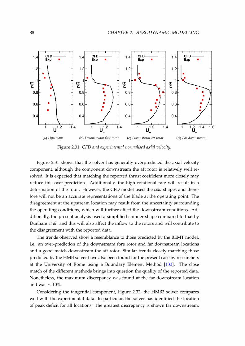
88 CHAPTER 2. AERODYNAMIC MODELLING
Un
r/R
1 1.2 1.4
0.4
0.6
0.8
1
1.2
1.4 CFDExp
(a) Upstream
Un
r/R
1 1.2 1.4
0.4
0.6
0.8
1
1.2
1.4 CFDExp
(b) Downstream fore rotor
Un
r/R
1 1.2 1.4
0.4
0.6
0.8
1
1.2
1.4 CFDExp
(c) Downstram aft rotor
Un
r/R
1 1.2 1.4 1.6
0.4
0.6
0.8
1
1.2
1.4 CFDExp
(d) Far downstream
Figure 2.31: CFD and experimental normalised axial velocity.
Figure 2.31 shows that the solver has generally overpredicted the axial velocitycomponent, although the component downstream the aft rotor is relatively well re-solved. It is expected that matching the reported thrust coefficient more closely mayreduce this over-prediction. Additionally, the high rotational rate will result in adeformation of the rotor. However, the CFD model used the cold shapes and there-fore will not be an accurate representations of the blade at the operating point. Thedisagreement at the upstream location may result from the uncertainty surroundingthe operating conditions, which will further affect the downstream conditions. Ad-ditionally, the present analysis used a simplified spinner shape compared to that byDunham et al. and this will also affect the inflow to the rotors and will contribute tothe disagreement with the reported data.
The trends observed show a resemblance to those predicted by the BEMT model,i.e. an over-prediction of the downstream fore rotor and far downstream locationsand a good match downstream the aft rotor. Similar trends closely matching thosepredicted by the HMB solver have also been found for the present case by researchersat the University of Rome using a Boundary Element Method [133]. The closematch of the different methods brings into question the quality of the reported data.Nonetheless, the maximum discrepancy was found at the far downstream locationand was ∼ 10%.
Considering the tangential component, Figure 2.32, the HMB3 solver compareswell with the experimental data. In particular, the solver has identified the locationof peak deficit for all locations. The greatest discrepancy is shown far downstream,

2.2. HIGH-ORDER AERODYNAMIC MODELLING 89
where the solver has predicted an almost cancellation of the tangential component,which is not demonstrated in the reported data. This disagreement may be attributedto the current matching to the reported loading and the difference in hot and coldrotor shapes.
Vn
r/R
0.2 0 0.2
0.4
0.6
0.8
1
1.2
1.4 CFDExp
(a) Upstream
Vn
r/R
0.2 0 0.2
0.4
0.6
0.8
1
1.2
1.4 CFDExp
(b) Downstream fore rotor
Vn
r/R
0.2 0 0.2
0.4
0.6
0.8
1
1.2
1.4 CFDExp
(c) Downstram aft rotor
Vn
r/R
0.2 0 0.2
0.4
0.6
0.8
1
1.2
1.4 CFDExp
(d) Far downstream
Figure 2.32: CFD and experimental normalised tangential velocity.
Finally, the radial component, Figure 2.33, is considered. Note that no upstreamradial component was presented by Dunham et al.. The HMB3 solver has again beenable to identify the location of peak deficit. However, there is a difference in thecompared magnitude of this deficit. Furthermore, the experimental data shows areduced radial component inboard of the tip vortex in comparison to the predictedvalues. Far downstream the computed results show a deficit in the near-hub region,likely a result from the hub gap. This deficit is not a physical solution and is known apriori due to the requirements of the Chimera implementation. This area is, therefore,neglected.
A validation study has been undertaken to verify the prediction capability of theHMB3 CFD solver. Upon comparison, the solver is generally capable of predictingthe velocity components and their development through the rotors and downstream.However, a number of discrepancies were observed. These discrepancies may beattributed to the unmatched loading and the fact that the cold rotor shape was mod-elled and uncertainties surrounding the inflow. Furthermore, the discrepancies ob-served may be further attributed to the unknown accuracy of the reported data. Theclose agreement between the HMB and a number of additional methods further sup-port this. Nevertheless, the HMB solver has been able to identify key features of the

90 CHAPTER 2. AERODYNAMIC MODELLING
CROR flowfield not possible with the low-order analysis.
Wn
r/R
0.4 0.2 0 0.2
0.4
0.6
0.8
1
1.2
1.4 CFDExp
(a) Downstream fore rotor
Wn
r/R
0.4 0.2 0 0.2
0.4
0.6
0.8
1
1.2
1.4 CFDExp
(b) Downstram aft rotor
Wn
r/R
0.2 0 0.2
0.4
0.6
0.8
1
1.2
1.4 CFDExp
(c) Far downstream
Figure 2.33: CFD and experimental normalised radial velocity.
Turbulence Performance
CROR flow is naturally highly turbulent, with high levels of vorticity in the rotorwake. The HMB3 solver offers a range of turbulence closures when solving theflowfield §2.2.3. Therefore, in order to asses the effect of turbulent model choice onthe CROR flowfield predictions, a turbulence study has been performed.
For the turbulence study, the k-ω, k-ω-SST and SST-SAS models have been used inthe prediction of the CROR flowfield. In particular, the turbulence models are com-pared for the validation test case. The experimental data presented no information onthe turbulent properties of the setup. In particular, it is unclear whether a trip devicewas use to trigger a fully turbulent boundary layer across the blade. Therefore, giventhe complexity of predicting transition, and the lack of information on the transitionbehaviour of this complex case, no transition turbulence models have been used inthis work. However, this may be an important feature for future analysis where moredetails of transition behaviour is available.
To compare the turbulence models, the flowfield upstream, downstream the forerotor, downstream the aft rotor and far downstream have been studied. Figures 2.34, 2.35and 2.36 respectively show the radial variation in the three components of velocityfor each turbulence model.
Comparing the axial component, Figure 2.34 shows that, with the exception of

2.2. HIGH-ORDER AERODYNAMIC MODELLING 91
far downstream, all three turbulence models predict very similar velocity profiles atall axial locations. For the far downstream location, the SST and k-ω models closelymatch in predicted profile. However, the SAS model predicts a higher peak velocityand a greater wake contraction. However, this increases the discrepancy with theexperimental data.
The tangential velocity comparisons, Figure 2.35, shows very close agreementbetween all models. All three models closely match in magnitude and location of thepeak deficit.
Comparison of the radial component, Figure 2.36, shows the most significantdifference between the three models. All models agree in the upstream direction,predicting no influence of the rotors on the upstream direction. In the downstreamfore and downstream aft locations, the models agree very well in the region of thepeak deficit. However, the magnitude of the peak deficit differs between the RANSmodels and the SAS. While the k − ω and SST models predict similar deficits, theSAS model shows a reduced deficit. Further investigation showed an increased eddyviscosity ratio and modelled turbulent kinetic energy for the RANS models. In thefar downstream region, the SAS model varies more significantly from the two RANSbased models.
A turbulence study has been carried out to investigate the performance of threeturbulence models implemented within the HMB solver. The results indicate thatthe RANS approaches followed the experimental trends more closely. Nonetheless,the differences predicted by the SAS approach were only small. The small differ-ences suggest that the SAS model mostly behaved like the RANS models and onlyhad small areas where the additional source term QSAS was activated. The acousticimpact of the three turbulence models will be further assessed in a later chapter inorder to inform the most suitable choice for the CROR analysis.

92 CHAPTER 2. AERODYNAMIC MODELLING
Un []
r/R
[]
0.9 1 1.1 1.2 1.30.2
0.4
0.6
0.8
1
1.2
1.4kωSSTSAS
(a) Upstream
Un []
r/R
[]
1 1.2 1.40.2
0.4
0.6
0.8
1
1.2
1.4kωSSTSAS
(b) Downstream fore rotor
Un []
r/R
[]
1 1.2 1.40.2
0.4
0.6
0.8
1
1.2
1.4kωSSTSAS
(c) Downstream aft rotor
Un []
r/R
[]
1 1.2 1.4 1.60.2
0.4
0.6
0.8
1
1.2
1.4kωSSTSAS
(d) Far downstream
Figure 2.34: Normalised axial velocity for each turbulence model.
Vn []
r/R
[]
0.2 0 0.20.2
0.4
0.6
0.8
1
1.2
1.4kωSSTSAS
(a) Upstream
Vn []
r/R
[]
0.2 0 0.20.2
0.4
0.6
0.8
1
1.2
1.4kωSSTSAS
(b) Downstream fore rotor
Vn []
r/R
[]
0.2 0 0.20.2
0.4
0.6
0.8
1
1.2
1.4kωSSTSAS
(c) Downstream aft rotor
Vn []
r/R
[]
0.2 0 0.20.2
0.4
0.6
0.8
1
1.2
1.4kωSSTSAS
(d) Far downstream
Figure 2.35: Normalised tangential velocity for each turbulence model.

2.2. HIGH-ORDER AERODYNAMIC MODELLING 93
Wn []
r/R
[]
0.1 0 0.10.2
0.4
0.6
0.8
1
1.2
1.4kωSSTSAS
(a) Upstream
Wn []
r/R
[]
0.2 00.2
0.4
0.6
0.8
1
1.2
1.4kωSSTSAS
(b) Downstream fore rotor
Wn []
r/R
[]
0.2 00.2
0.4
0.6
0.8
1
1.2
1.4kωSSTSAS
(c) Downstream aft rotor
Wn []
r/R
[]
0 0.20.2
0.4
0.6
0.8
1
1.2
1.4kωSSTSAS
(d) Far downstream
Figure 2.36: Normalised radial velocity for each turbulence model.
2.2.6 HMB execution
With the large grid sizes required to compute the CROR flowfield, High-PerformanceComputing (HPC) resources were required to execute the HMB3 solver. Throughoutthe project, a number of HPC resources have been used. In particular, the ManchesterHPC pool [134], the Tier 2 Cirrus HPC [135] and the former N8 Polaris HPC facil-ity [136] were all utilised for running CROR simulations. Simulations were typicallycarried out on 500-540 cores. Due to the grid configuration (cell count per block),further cores would achieve no reduction in computing time.
To avoid high gradients in the initial stages of the unsteady simulations, the ro-tational speed is gradually increased from zero to the required speed over a singlerotation. Furthermore, a coarser temporal resolution is used in the first two revo-lutions before being reduced to the required value. At least 4 rotor rotations wererequired to obtain statistical time-invariance of the flow variables, after which flow-field data were recorded over a further complete rotor revolution.
This sub-section has introduced a high-order approach for computing CROR aero-dynamic performance. The governing equations of fluid flow have been introducedin terms of the HMB3 CFD solver. Furthermore, pre-processing requirements forthe particular case of CROR has also been introduced. The solver has been shownto agree relatively well with reported data. Both mesh independence and turbu-lence modelling have been studied to verify the solvers performance further. The

94 CHAPTER 2. AERODYNAMIC MODELLING
high-order approach offers greater detail of the flow-physics in comparison to thelow-order models, thus allowing for a greater understanding of the underlying noisegenerating mechanisms.
2.3 Summary
This section has introduced both low- and high-order modelling techniques forthe analysis of CROR aerodynamic performance. Both methodologies were com-pared against available experimental data, showing sufficient accuracy for the workcarried out in the thesis. Furthermore, a sensitivity analysis was carried out for eachapproach to verify their respective predictions further and understand the pertinentpreprocessing procedures and input data.
The low-order models, while not suitable for a detailed understanding of theflow-physics, are extremely useful as a design tool due to their low computationalcost. On the other hand, the high-order models are not yet suitable as design toolsdue to their onerous computational cost. However, they remain important to betterunderstand the flow features and improve existing models.

Chapter 3
Aeroacoustic Modelling
The most significant component of aircraft noise is that due to the propulsionsystem, and this is especially true for propeller-driven aircraft. In an effort to in-vestigate the aeroacoustic emissions of propellers, this chapter presents both low-and high-order strategies for computing propeller and CROR noise. A descriptionof the various noise sources which contribute to rotor noise is first introduced. Fol-lowing this, both low- and high-order modelling of CROR noise is discussed. Bothmethodologies are accompanied by a validation and sensitivity study.
3.1 Rotor Noise Sources
The theory of propeller noise was first investigated by Lynam and Webb [137].However, the advancements of Gutin [138] are perhaps of the greatest significance.Gutin presented a theoretical development of the noise due to the rotating forcesproduced by the propeller and was shown to agree reasonably well with experimentalpredictions [139]. Significant advancements in the theory and understanding of thenoise sources have since been made. It is the work of Lighthill [140] however, forwhich most modern aeroacoustic models are based [141]. The work of Lighthillhas been developed further by Ffowcs Williams and Hawkings [142] to allow foreasier numerical implementation of the noise sources, particularly for the case here ofpropellers. The Ffowcs Williams Hawkings equations form the basis of most modernrotor noise codes for both low- and high-order methods.
CROR noise poses a complex problem; it is highly tonal with significant noisein all directions over a wide frequency range. CROR noise comprises a number ofsources. These sources are summarised in Figure 3.1.
95

96 CHAPTER 3. AEROACOUSTIC MODELLING
CROR-Noise
Steady Loading(Tonal) Broadband
Thickness Loading
UnsteadyLoading
Non-Linear (quadrupole)
PotentialInteractions Wake Inteactions
Trailing Edge R-R Interaction
Figure 3.1: CROR noise sources.
Tonal Noise
Tonal noise is harmonic in nature, i.e. it is periodic. In the time domain, it canbe represented by a constant rate pulse. For a rotor with N blades and rotationalfrequency n, the tonal noise will appear as a peak at the fundamental Blade PassageFrequency, BPF = nN, in the frequency domain. The noise will then linearly decreaseat integers of the BPF. Characteristic time and frequency responses of steady noiseare shown in Figure 3.2.
Figure 3.2: Rotor steady noise characteristics (adapted from [21]).
Steady noise sources are typically grouped as thickness noise and loading noise.Thickness noise results from the volume displacement of the fluid as the rotor rotates.The resulting noise is proportional to the blade volume, with the frequency responsecharacterised by the aerofoil shape [21] and can be represented as a monopole source.
Loading noise results from the pressure field caused by the aerodynamic loadingas the rotor rotates. The loading source can be represented by a dipole. The loadingcontribution is proportional to the lift and drag (or thrust and torque) produced bythe blade. For low-speed conditions, the loading terms typically dominate e.g. take-off. For increasing speeds, the thickness terms become more important, e.g. duringcruise.

3.1. ROTOR NOISE SOURCES 97
Quadrupole Noise
For low to moderate speeds, the steady sources are linear. However, as the flowover the rotor becomes transonic, the noise becomes non-linear, and instead of actingon the blade surface, the volume around the blade needs to be considered. Thisnon-linear noise can be characterised as a quadrupole source. Modelling of thequadrupole source requires properties of the transonic flow. However, for generalaviation propellers, where the tip speed remains low, the quadrupole source is unim-portant.
Broadband Noise
Broadband noise results from the random turbulent fluctuations throughout theflow. For a rotor, there are two sources of broadband noise [21]. Firstly, leading-edge broadband noise results from the ingestion of turbulent flow by the rotor. Themagnitude of the resulting noise is proportional to the level of turbulence in the flow.This may result from natural turbulence of the flow or for example, from an upstreampylon. This source of broadband noise is also important in the case of CROR, wherethe aft rotor interacts with the turbulent flow created by the fore rotor [143].
Trailing-edge broadband noise is the second source of rotor broadband noise. Theturbulent boundary layer present for most rotors will result in a fluctuation in loadsthat terminate at the blade trailing edge. The resulting noise is dependant on theproperties of the rotor boundary layer. Figure 3.3 presents typical broadband noiseresponses in both time and frequency domains.
Figure 3.3: Rotor steady noise characteristics (adapted from [21]).
Unsteady Loading Noise
Non-axial flight, interaction with an upstream disturbance and rotor installationall give rise to unsteady loading noise. The unsteady loading on the rotor contributesto noise at the rotor harmonics. Furthermore, the circumferential directivity is no

98 CHAPTER 3. AEROACOUSTIC MODELLING
longer axisymmetric and now appears as a number of lobes. The number of lobes isproportional to the order or frequency of the unsteady loading.
For CROR, the interaction between fore and aft rotors results in periodic loadingon both rotors and, therefore, unsteady loading noise. Figure 3.4 shows the CROR in-teraction mechanisms that result in unsteady loading noise. Unsteady loading noisecan be a significant source for the CROR, typically dominating for low-speed opera-tions (e.g. take-off and climb-out) [144].
Figure 3.4: CROR interactions resulting in unsteady loading.
The unsteady aerodynamic loading on each rotor will be periodic with respect tothe opposing rotor. As a result of the periodic loading, the CROR noise spectrum willconsist of the rotor alone tones occurring at BPF1 and BPF2 and the so-called interac-tion tones: k1n1N1± k2n2N2 (∀k1,k2,∈Z), i.e. the sum and difference tones. The CRORfrequency spectrum, unlike the rapid decay seen for isolated rotors, is characterisedby high amplitudes across the spectrum. Furthermore, during flyover scenarios, theCROR is shown to produce high noise levels near the axis of rotation, unlike the iso-lated rotor, which rapidly decays away from the rotor plane. The unsteady loadingsource is, therefore, an important source that cannot be neglected when consideringCROR noise.
3.2 Noise Metrics
Whilst sound represents the physical pressure perturbations in the flow, noisedescribes the perception of this sound by the human ear [145] (although both aretypically used interchangeably). Therefore, due to the subjective nature of noise,it can be difficult to quantify. As a result of this, a number of metrics have beendeveloped to account for various properties of the sound. In this section, a number

3.2. NOISE METRICS 99
of common metrics which have been used throughout this work are introduced.
The human ear is able to perceive a large dynamic range, It can generally detectsound pressures in the range of 20 µPa→ 200 Pa [146]. Given the large range inacoustic pressure, it is typical to work on a logarithmic scale. As a result, the SoundPressure Level (SPL) is defined:
SPL = 20log10(p/pre f ), (3.1)
where pre f is taken as 20µPa and represents the threshold of human hearing. The earis capable of discerning ±1 dB, whilst ±10dB results in a noticeable difference in thesound level. As the scale is logarithmic, a doubling of the sound pressure results ina ∼ 6 dB difference in sound level [147].
Noise is typically recorded and analysed as a signal (over a period of time), asopposed to a single event. Therefore, the sound pressure level of the signal is givenby:
SPL = 20log10(prms/pre f ), (3.2)
prms is the root-mean-squared of the pressure signal.
The human ear can also perceive a large frequency range from around 20 Hz→20 kHz. However, it is not equally sensitive to all frequencies [148]. As a result, it istypical to employ some weighting to a noise signal. The A-weighting is commonlyused for environmental measurements. However, it is also used in the certificationof general aviation Aircraft (light propeller-driven aircraft with a maximum take-off mass < 8,618 kg) [149]. The A-weighting is applied to account for the relativeperception across frequencies of the ear (i.e. it is less sensitive for low-frequencies). A-weighting is graphically shown in Figure 3.5. The A-weighted SPL can be computedaccording to [150]:
LA( f ) = SPL( f ) + 20log10(GA( f )) + 2 dB(A), (3.3)
where GA is the filter gain:
GA( f ) =121942 f 4
(20.62 + f 2)(107.72 + f 2)12 (737.92 + f 2)
12 (121942 + f 2)
(3.4)
For larger commercial aircraft, the EPNL metric is used for noise certification [151].The EPNL is a weighted, integral metric. It is corrected for the tonal content of thesignal and can account for the duration and loudness of the sound. The computationof the EPNL is a cumbersome exercise. Therefore, the reader is directed towardsRefs. [145, 147] which detail the required process. The EPNL is a single number

100 CHAPTER 3. AEROACOUSTIC MODELLING
representing the noise over a single aircraft operation, it is calculated from flyovermeasurement and cannot be directly measured.
Frequency, f [Hz]
GA(f
) [
dB
]
101
102
103
104
60
50
40
30
20
10
0
10
AWeighting
Figure 3.5: A-weighting frequency gain.
3.3 Low-Order Noise Modelling
There is a wide range of theories for describing rotor noise. To be used as asuitable design tool, the theory must provide sufficient physical detail at a low com-putational cost. To this end, this section introduces the low-order noise model whichhas been used throughout this work.
Steady Noise
To unify the various noise sources and unsteady loading terms, the analysisthroughout this work utilises a frequency domain approach. Many authors havepreviously reported the expression for the steady noise of an isolated rotor [152, 153,40, 21]. The acoustic pressure at observer location xxx and time t due to the rotor is
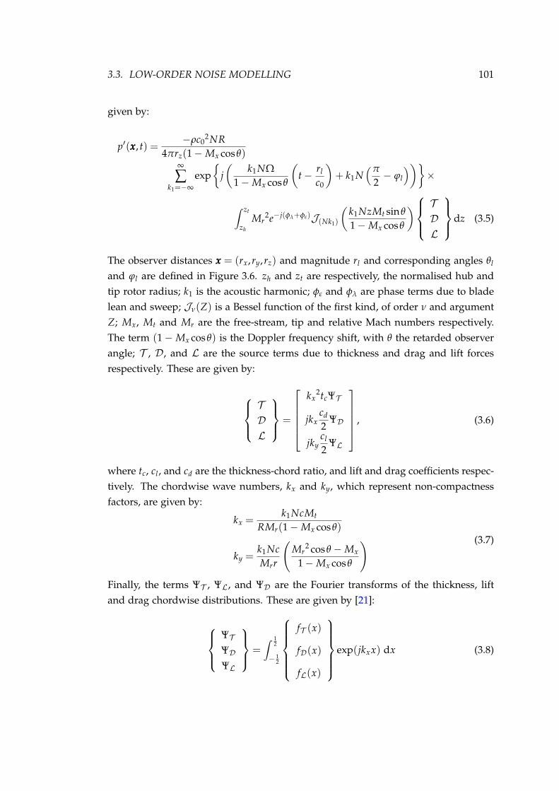
3.3. LOW-ORDER NOISE MODELLING 101
given by:
p′(xxx, t) =−ρc0
2NR4πrz(1−Mx cosθ)
∞
∑k1=−∞
exp
j(
k1NΩ1−Mx cosθ
(t− rl
c0
)+ k1N
(π
2− ϕl
))×
∫ zt
zh
Mr2e−j(φλ+φε)J(Nk1)
(k1NzMt sinθ
1−Mx cosθ
)TDL
dz (3.5)
The observer distances xxx = (rx,ry,rz) and magnitude rl and corresponding angles θl
and ϕl are defined in Figure 3.6. zh and zt are respectively, the normalised hub andtip rotor radius; k1 is the acoustic harmonic; φε and φλ are phase terms due to bladelean and sweep; Jν(Z) is a Bessel function of the first kind, of order ν and argumentZ; Mx, Mt and Mr are the free-stream, tip and relative Mach numbers respectively.The term (1−Mx cosθ) is the Doppler frequency shift, with θ the retarded observerangle; T , D, and L are the source terms due to thickness and drag and lift forcesrespectively. These are given by:
TDL
=
kx
2tcΨT
jkxcd
2ΨD
jkycl
2ΨL
, (3.6)
where tc, cl , and cd are the thickness-chord ratio, and lift and drag coefficients respec-tively. The chordwise wave numbers, kx and ky, which represent non-compactnessfactors, are given by:
kx =k1NcMt
RMr(1−Mx cosθ)
ky =k1NcMrr
(Mr
2 cosθ −Mx
1−Mx cosθ
) (3.7)
Finally, the terms ΨT , ΨL, and ΨD are the Fourier transforms of the thickness, liftand drag chordwise distributions. These are given by [21]:
ΨTΨDΨL
=∫ 1
2
− 12
fT (x)
fD(x)
fL(x)
exp(jkxx) dx (3.8)

102 CHAPTER 3. AEROACOUSTIC MODELLING
where, fT (x), fD(x), and fL(x), describe the thickness and loading distributionsalong the blade section chord. As the chordwise loading is not available from theBEMT approach, an analytical expression assuming a uniform loading distributioncan be used [21]:
fD(x) = 1
fL(x) = 1
−1
2≤ x ≤ 1
2(3.9)
which gives:
ΨL = ΨD =
1 (kx = 0)
2kx
sin(
kx
2
)(kx 6= 0)
(3.10)
The assumption of uniform loading should be sufficient for the rotors consideredthroughout this work [18].
Studying the above expression gives some preliminary insight into the behaviourof rotor noise. The first exponential term in Equation (3.5) describes the propertiesof the radiating sound field. The term rl/c0 − t indicates the acoustic waves willpropagate radially outwards at sound speed, c0 [21]. The term k1Nϕl illustrates thatpeak noise will be heard at frequencies of k1N Ω
2π , i.e. at multiples of BPF. It alsoshows that circumferential directivity, which will rotate with the propeller at it’sangular velocity, will have lobes proportional to k1N. The terms to the right of theintegral consist of the source terms, T , D, and L, and the Bessel function. This Besselfunction characterises the radiation efficiency of the acoustic pressure [29]. Where theBessel function decays more rapidly for increasing order, ν. The source terms affectthe magnitude of the acoustic pressure.
Further insight can be gained by carrying out a dimensional analysis of the aboveexpression for the rotor noise dependence on the local blade velocity. Firstly theexponential terms are neglected Following this, the Bessel function term can also beneglected as for subsonic flows (as considered here) the argument will be less thanthe order. This leaves the following expression:
p′ ∝−ρc0
2NR4πrz(1−Mx cosθ)
Mr2
TDL
(3.11)
Expanding the source terms for all components, including the wave numbers revealsthat the thickness and drag components have a dependence of Mr
2 whilst the liftcomponent has the dependence of Mr
3 (due to the additional Mach number term inky). For the thickness and loading terms these are the classical velocity relations formonopole and dipole sources respectively [154, 155].
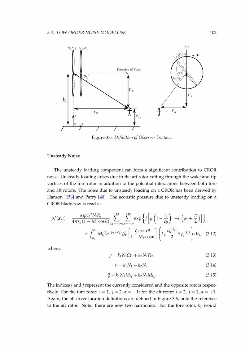
3.3. LOW-ORDER NOISE MODELLING 103
x
z
Aft
2
N2, 2 N1, 1
Figure 3.6: Definition of Observer location.
Unsteady Noise
The unsteady loading component can form a significant contribution to CRORnoise. Unsteady loading arises due to the aft rotor cutting through the wake and tipvortices of the fore rotor in addition to the potential interactions between both foreand aft rotors. The noise due to unsteady loading on a CROR has been derived byHanson [156] and Parry [40]. The acoustic pressure due to unsteady loading on aCROR blade row is read as:
pi′(xxx, t) =
αjρc02NiRi
4πrz (1−Mx cosθ)
+∞
∑k1=−∞
+∞
∑k2=−∞
exp
j[
µ
(t− rl
c0
)+ν(
ϕl +π
2
)]×∫ zti
zhi
Mri2ej(φλ+φε)Jν
[ξzi sinθ
1−Mx cosθ
]kyi
cli(k j)
2ΨLi
(k j)
dzi, (3.12)
where,µ = k1N1Ω1 + k2N2Ω2, (3.13)
ν = k1N1 − k2N2, (3.14)
ξ = k1N1Mt1 + k2N2Mt2 . (3.15)
The indices i and j represent the currently considered and the opposite rotors respec-tively. For the fore rotor: i = 1, j = 2, α = −1; for the aft rotor: i = 2, j = 1, α = +1.Again, the observer location definitions are defined in Figure 3.6, note the referenceto the aft rotor. Note: there are now two harmonics. For the fore rotor, k1 would
104 CHAPTER 3. AEROACOUSTIC MODELLING
be the acoustic harmonic, whilst k2 would be the loading harmonic. With the oppo-site being true when considering the aft rotor. The non-dimensional wave numbers(again characterising non-compactness) are, in this case, given by:
kxi =ci
Ri Mri
[ξ
1−Mx cosθ− k jNj(Mt1 + Mt2)
], (3.16)
kyi =−αci
Ri Mri
[ξMti zi cosθ
1−Mx cosθ+ α
νMx
zi
]. (3.17)
Quadrupole Noise
When the relative velocity of the rotor blade approaches transonic speeds, the lin-ear loading terms become non-linear. This can be represented as a quadrupole source.To model this source requires details of transonic flow perturbations. Obtaining thesedetails can be computationally expensive and as a result, would be out of the scopeof a low-order analysis. Furthermore, in this work, the focus is on general aviationaircraft, where even during cruise, the rotors do not reach transonic speeds. As aresult of this, the quadrupole term is not modelled in the present work. However, fora more in-depth review of the quadrupole source as well as modelling strategies, thereader is directed towards the works of Hanson & Fink [157] and Parry [158].
Broadband Noise
Broadband noise is typically characterised as being lower in amplitude than thetonal component. However, whilst the tonal component is significant at a few dis-tinct harmonics, the broadband component is distributed across the whole frequencyspectrum. It has also been shown that in some cases the broadband component canbe as important as the tonal contribution for CROR [159].
Due to the nature of broadband noise, i.e. it is based on turbulent, and hence, ran-dom fluctuations, it can be difficult to compute. As discussed previously for CROR,there are two components of the broadband noise, the leading-edge component (dueto rotor-rotor interaction) and the trailing-edge component. The equations describ-ing the broadband component are typically exhaustive, containing many terms, inparticular those describing the aerodynamic behaviour of the turbulent flow. As aresult, the equations are fully described in Appendix A. Only the leading equationsare shown here.
There are a number of models to compute the trailing-edge broadband compo-nent. The model described by Magliozzi et al. [21] is simple to use and is relativelyaccurate at predicting the broadband noise due to scattering of the turbulent bound-ary layer [147]. The model described by Magliozzi et al. is based on the work of

3.3. LOW-ORDER NOISE MODELLING 105
Amiet [160] on broadband noise on a flat plate. From Magliozzi et al. the far-fieldnoise spectrum is read as:
Spp(xxx,ω) =
(ωbz
2πc0σ2
)2
ly(ω)s|L|2Sqq(ω,0), (3.18)
The second component of broadband noise from a CROR arises due to the tur-bulent interaction as the aft row interacts with the wake of the fore row. This isdescribed as rotor-rotor broadband interaction noise. For the analysis, the modelpresented by Kingan [161] is used. This model is an updated model based on theoriginal work of Blandeau [162].
From Kingan, the time-averaged rotor-rotor broadband pressure spectrum is givenby:
SppRR(xxx,ω) =∞
∑k1=−∞
∞
∑k2=−∞
2πN2
(4πRe)2(1−M cosθ)2
∫ Rt
Rh
(πVr2
ln(2)
)(ρN1b1/2
r cosα1
)2
G(kb)2S2J 2
n
(κr sinθ
1−M cosθ
)×
Φ(2)ww(KX2 eeeX2)|ΨL(KX2 ,0,ω− nΩ2,kc)|2dr. (3.19)
Recall, the above equations are fully presented in Appendix A. The equations for thecomputation of the broadband source are given in a strip formulation. In particular,the equations are computed for each observer location for a given frequency andblade span discretisation. Therefore, it is convenient to code them in a matrix formto reduce the computational cost.
3.3.1 Model Validation
In order to verify the prediction of the CROR noise model, it should be comparedagainst a number of experimental data sets. Despite the scarcity of data in the openliterature, a small number of sources have been found with which to compare theCROR code. The code is first compared against the case of an isolated rotor beforeconsidering a CROR cases.
SR2 SRP
Block [163] investigated the noise from an isolated 4 bladed SRP at two operatingpoints. The first case considers the rotor at a setting angle of 20.6o rotating at 120rev/s. In the second case, the rotor is at a setting angle of 12.7o, rotating at 168 rev/s.In both cases, the freestream velocity is ∼30 m/s. Figure 3.7 compares the reported

106 CHAPTER 3. AEROACOUSTIC MODELLING
and computed Overall Sound Pressure Level (OASPL) for the two SRP operatingcases.
Polar Angle, θ [deg]
OA
SP
L [
dB
]
50 100 15060
70
80
90
100
ModelExp
(a) β.75 = 20.6, n = 120 rev/s
Polar Angle, θ [deg]
OA
SP
L [
dB
]
50 100 15080
90
100
110
ModelExp
(b) β.75 = 12.7, n = 168 rev/s
Figure 3.7: SRP noise prediction.
Figure 3.7 demonstrates that the acoustic model predicts well the OASPL of theSRP in both cases. There are some discrepancies towards the extremes of the ob-server angles. However, this was also found in numerical comparisons by Block [163]and is described as possibly being caused by nacelle diffraction as the polar angleapproaches the rotor axis.
SR2 CROR
Directivity trends for a 0.409 m 4× 4 scale CROR have been presented by Block [164].With both rotors rotating at n∼ 192 rev/s, Block presented trends up to the third har-monic of BPF. The CROR noise was measured at a number of azimuthal and polarangles, Figure 3.8. However, the data was presented as polar directivities, havingbeen averaged over the azimuthal component. To match the reported data, this aver-aging was done according to:
SPL(θ, f ) = 10log
(1m
m
∑i=1
10SPL(θ,ψi , f )
10
)(3.20)
where m is the number of azimuthal microphone positions, here 22.Figure 3.9 compares the OASPL and SPL of the first three harmonics reported by
Block [164] and those obtained using CROR noise model.

3.3. LOW-ORDER NOISE MODELLING 107
Figure 3.8: Microphone locations for CROR noise validation, adapted from Ref. [164].
Polar Angle, θ [deg]
OA
SP
L [
dB
]
50 100 150
80
90
100
110
120
HFWHExp
(a) OASPL
Polar Angle, θ [deg]
SP
L [
dB
]
50 100 150
80
90
100
110
120
HFWHExp
(b) BPF1
Polar Angle, θ [deg]
SP
L [
dB
]
50 100 150
80
90
100
110
120
HFWHExp
(c) BPF2
Polar Angle, θ [deg]
SP
L [
dB
]
50 100 150
80
90
100
110
120
HFWHExp
(d) BPF3
Figure 3.9: Comparison of computed and reported SPL values for SR2 CROR.
Figure 3.9 shows that the OASPL has been very well captured by the CROR noisemodel over the entire directivity. The first harmonic of BPF is relatively well capturedover the directivity. However, there is a slight discrepancy in the upstream direction.The second and third harmonics are not captured so well. There is good agreement

108 CHAPTER 3. AEROACOUSTIC MODELLING
in the overhead position, owing to the steady component. However, moving up-or downstream, there is a significant difference between the predicted and reporteddata. The reduced levels in the up- and downstream directions predicted by thenoise model suggest the unsteady interaction has not been captured so well. Thissuggests a deficiency in the aerodynamic interaction model. As the polar directivitiesare averaged over the azimuthal component, the discrepancies are more difficult toattribute. Nonetheless, the OASPL has been predicted very well and given the factthat the total noise is the useful component for the present analysis, the model haspredicted the CROR noise to a sufficient level of accuracy for the current work.
3.3.2 Sensitivity Analysis
In order to validate the CROR noise model, it has been compared against availableexperimental data. A sensitivity analysis has been undertaken to investigate potentialsources of the discrepancy. Furthermore, the sensitivity analysis will demonstratethe effect of small changes in various parameters on various noise sources. Thesensitivity analysis has been carried out on 3m diameter SRP and CROR rotatingat 1,000 rev/min, representing the characteristics of the rotors used in the analysisthroughout this work.
Rotor Thickness
The rotor blade thickness, or more precisely the blade volume, is the source ofrotor thickness noise. The thickness of the blade has been varied by ±10% to investi-gate the sensitivity of this noise source. This should also indicate if small differencesin thickness, e.g. from extracting the geometry will propagate to a large difference inthickness noise.
Figure 3.10 demonstrates the effect of rotor thickness on the resulting peak noiselevel of the thickness noise source. The relative velocity of the rotor throughoutthe sensitivity analysis is below transonic speeds and constant. The peak thicknessnoise is shown to vary by a maximum of ∼ ±0.9dB over the blade thickness rangetested. The characteristic parabolic arc representing a flyover was found to translatevertically for variations in blade thickness.
Extraction of the spanwise geometry may result in errors when representing thegeometry. However, these are likely to be small. Figure 3.10 demonstrates that theresulting change in SPL is therefore small and accuracy of the thickness should notbe a concern so long as the thickness of the section is accurate to a few per cent.

3.3. LOW-ORDER NOISE MODELLING 109
∆tc [%]
Th
ick
ne
ss
No
ise
, ∆
SP
Lt [d
B]
10 5 0 5 101
0.5
0
0.5
1
Figure 3.10: Effect of blade thickness on thickness noise.
Rotor Speed
The rotational speed of the rotor is known to have a significant effect on theresulting noise emission of the rotor. To quantify this effect, Figure 3.11 presents thechange in SPL of thickness and loading sources as well as the EPNL due to differencesin rotational speed. The investigation is carried out with the rotor delivering the samethrust for each rotational speed.
∆Ω [%]
∆S
PL
[d
B]
∆E
PN
L [
dB
]
10 5 0 5 10
4
2
0
2
4
5
0
5SPLSPL
tSPL
lEPNL
Figure 3.11: Effect of Rotational speed.
Figure 3.11 shows that the rotational speed has a greater effect on the thickness

110 CHAPTER 3. AEROACOUSTIC MODELLING
component than the loading component. For the loading component, the change inrotational speed will also affect the sectional loading (to keep the total blade thrustconstant) and hence will also affect the resulting noise source. Due to the dominanceof the loading component for the current case, the large change in the thicknesscontribution is not seen in the total noise changes. Nonetheless, the total noise isseen to change by more than 2 dB for a 10% change in rotational speed. Figure 3.11also shows that using an integral metric, here, EPNL, can change by as much as 5 dBfor a 10% change in rotational speed. Comparing the trends of thickness and loadingnoise, it is shown that they do not follow the relations: SPLT ∝ U4 and SPLL ∝ U6.However, these relations cannot be easily seen as the relative velocity varies alongthe blade span, and the effect of rotational velocity is compared here. For the loadingcomponent, it is further complicated as the source strength of each spanwise locationalso varies.
The analysis of the sensitivity of the rotor rotational speed has shown that theresulting noise is highly sensitive to the rotor rotational speed. The effect of rotationalspeed will be more important when the thickness component will dominate, e.g.during cruise. Therefore, for accurate noise prediction, the rotational speed must beprecisely replicated.
Accuracy of Aerodynamic data
The aerodynamic data used to trim the rotor is taken from 2D look-up tables orfrom linear approximations. To this end, it is important to understand the effects ofthe aerodynamic data on the resulting noise emissions. Given that the expression forthe loading noise is of the same form as the thickness component, it is expected tohave a similar response to changes in thickness. This response is shown in Figure 3.12,where the changes in peak SPL are shown for changes in the rotor lift coefficient foran isolated SRP. As the loading noise is dominant here, it is also possible to show theeffect on the integral metric, EPNL.
The response shows that the noise is directly proportional to the source strength,here cl . The same response was found for the drag coefficient. The EPNL also showsa dependency on the rotor aerodynamics. For both metrics, the maximum differenceis ∼ 1dB for the maximum changes in lift coefficient. While this does not seem like alarge change, a 1 dB change is equivalent to a ∼ 15% change in the acoustic pressure.Therefore, the accuracy of the aerodynamic predictions may have a significant impacton the resulting noise predictions.
CROR noise introduces an additional loading source — the noise due to un-steady loading. Therefore, the sensitivity of CROR noise to this source is investigated.The sensitivity analysis is applied by increasing/decreasing the unsteady component

3.3. LOW-ORDER NOISE MODELLING 111
equally across all harmonics. Figure 3.13 presents the effect of the harmonic loadingcomponent on the resulting noise of fore and aft rotors. The error bars represent amaximum change in the unsteady component of ±10%. The steady component isalso presented for reference.
∆cl [%]
∆S
PL
[d
B]
∆E
PN
L [
dB
]
10 5 0 5 101
0.5
0
0.5
1
1
0
1
SPLEPNL
Figure 3.12: Effect of steady aerodynamic component on peak and EPNL noise levels.
Polar Angle, θ [deg]
SP
L [
dB
]
50 100 15030
40
50
60UnsteadySteady
(a) Fore rotor
Polar Angle, θ [deg]
SP
L [
dB
]
50 100 15030
40
50
60UnsteadySteady
(b) Aft rotor
Figure 3.13: Effect of the unsteady loading component of CROR noise.
For both fore and aft rotors, Figure 3.13 shows that the importance of includingthe unsteady component as it has a significant effect on the resulting flyover profile.Figure 3.13 also demonstrates that the overhead position is dominated by the steady

112 CHAPTER 3. AEROACOUSTIC MODELLING
component of the noise, with both fore and aft unsteady components demonstratinglittle deviation from the steady component at this position.
It is shown that the greatest deviation in SPL is found near the axis of rotation.For the fore rotor, the greatest deviation is on the upstream side, whilst for the aftrotor, this is on the downstream side. The high SPL near the axis of rotation, whichis demonstrated for the aft rotor, is characteristic of CROR noise. Figure 3.13 suggesta maximum deviation of around 1dB for a ±10% change in the unsteady loading.Even with the lower bound, the profile still retains its characteristic shape.
To investigate the unsteady loading further, Figure 3.14 compares the effect ofunsteady loading changes for increasing harmonics of BPF at the overhead position(θ = 90). Figure 3.14 shows that the steady component rapidly decays, for the firstthree harmonics, this is also true for the unsteady component. However, for bothfore and aft rotors, the SPL then increases for increasing harmonics. As this is forthe overhead position, the steady component is dominant, as demonstrated by equalvalues of the steady and unsteady cases at the first harmonic. For positions awayfrom the rotor plane, the unsteady component is found to increase further for higherharmonics.
Harmonic of BPF []
SP
L [
dB
]
2 4 6 8 1020
25
30
35
40
45
50
55
60Unsteady Steady
(a) Fore rotor
Harmonic of BPF []
SP
L [
dB
]
2 4 6 8 1020
25
30
35
40
45
50
55
60Unsteady Steady
(b) Aft rotor
Figure 3.14: Harmonic components for steady and unsteady aerodynamics at overheadposition, θ = 90.
The maximum deviation for the unsteady component is around 1dB for the max-imum ±10% change in the unsteady component. This difference does not change theoverall trends observed but may become significant when integrating across the spec-trum. Furthermore, the results have demonstrated that the accuracy of the unsteady

3.3. LOW-ORDER NOISE MODELLING 113
component has a significant impact on the resulting noise.
Overall, the sensitivity analysis of the unsteady loading component has demon-strated that and equal change in the harmonics resulted in a significant change in SPLalong the flyover. Therefore, this may be a cause for an underprediction observed forthe second and third harmonics in the validation cases.
Time Discretisation
The equations presented above require a discretisation of time for computationof the rotor noise. This discretisation results in a complete rotor revolution beingdivided into a number of time or azimuth steps. The resulting time step dictates howmany points are used to describe the time signal or the sampling frequency of thenoise and the maximum frequency that can be resolved. Therefore, the choice of timediscretisation is problem dependant.
Ideally, the greatest time discretisation should be used to resolve the highest fre-quencies, or at least up to the upper range of audible frequencies. However, this isoften not possible whilst minimising computational cost. As a result, a sensitivityanalysis of the time discretisation has been undertaken. The case of a SRP at take-offconditions (M = 0.2, Ω = 1,000 rev/min) has been simulated as this is representativeof the analysis throughout this thesis. A SRP has been used to reduce the number ofresulting variables (i.e. the noise of a single rotor as opposed to two).
Figure 3.15 demonstrates the effect of increasing time discretisation on the result-ing EPNL and maximum A-weighted SPL in a simulated constant-altitude flyover.These metrics have been used as they operate on amplitudes within frequency bandsand are, therefore, much more greatly affected by the frequency resolution. Fig-ure 3.15 shows that for an increasing number of time points, the resulting EPNL andLAmax rapidly converge to a final value. While the noise metrics rapidly converge,the resulting computational time exponentially increases. Therefore, a compromiseon acceptable accuracy and computational time must be made. From the sensitivityanalysis, a time discretisation of 1,000 points was chosen. The use of 1,000 pointsresults in a difference of only 0.28 dB from the converged value obtained using 5,000time points whilst reducing the computational time by 123%∗. Whilst using 5,000points does not represent a significant computational time itself, the objective of thelow-order models is to minimise the computational cost. Furthermore, the use of1,000 points results in ∼ 8,000Hz to be resolved, > 100 times the BPF, which is muchmore than is interesting.
∗Computations carried out on a single Intel R© CoreTM i7-6700 CPU

114 CHAPTER 3. AEROACOUSTIC MODELLING
Time Discretisation
EP
NL
[d
B]
LA
ma
x [
dB
]
101
102
103
104
105
106
40
44
48
52
33
35
37
39
41
EPNLLA
max
(a) Computed noise
Time DiscretisationT
CP
U [
s]
Tw
all [
s]
101
102
103
104
105
10610
1
100
101
102
103
102
101
100
101
102
TCPU
T
wall
(b) Computation time
Figure 3.15: Effect of time discretisation.
3.4 High-Order Noise Modelling
A high-order aeroacoustic analysis is performed based on detailed flow-field datafrom high-order aerodynamic tools. Therefore, the modelling should be able to cap-ture a greater detail of the flow physics and the resulting noise emissions.
Two approaches are available to utilise CFD data for CROR noise predictions.Either a porous surface or a solid-surface formulation can be used. A comparisonof the two approaches is described in Ref. [165]. A solid-surface formulation is usedthroughout this work.
3.4.1 Farassat 1A Code
The Farassat 1A formulation [153] of the original Ffowcs Williams-Hawking equa-tion [142] was implemented to calculate rotor noise based on blade surface pressurescomputed form uRANS CFD simulations using the HMB solver. The Farassat formu-lation is given by a summation of thickness and loading contributions:
p′(xxx, t) = pL′(xxx, t) + pT
′(xxx, t) (3.21)

3.4. HIGH-ORDER NOISE MODELLING 115
where,
4πpT′(xxx, t) = ρc0
∫f=0
[Mn
R(1−Mr)2 +Mn Mr
R(1−Mr)3
]ret
dS+
ρc0
∫f=0
[c0Mn(Mr −M2)
R2(1−Mr)3
]ret
dS (3.22)
and
4πpL′(xxx, t) =
∫f=0
[pS cosΘ
c0R(1−Mr)2 +Mr pS cosΘR(1−Mr)3
]ret
dS+∫f=0
[pS(cosΘ−Mn)
R2(1−Mr)2 +pS cosΘ(Mr −M2)
R2(1−Mr)3
]ret
dS (3.23)
Note that the quadrupole source has been neglected in the present work. The 1R
terms in both thickness and loading terms represent the far-field component, whilethe 1
R2 terms describe the near-field components.
M is the Mach number, with subscripts r and n representing the Mach numberin radiation and normal direction respectively, with r and n the unit radiation andnormal vectors respectively. Θ is the angle between the normal and radiation vectors.R is the magnitude of the radiation vector, r. Finally, pS is the pressure on the bladesurface, S.
Blade surface pressure is extracted at each time step to compute the noise. Eachblade is discretised into a number of panels from which the surface pressure is ex-tracted and appended to an input file. From the local panel velocities and surfacepressures, the acoustic pressure can be calculated for each radial and chordwise po-sition on the blade. The source-dominant implementation of the Farassat formulationis used in the present work. In the source-dominant approach, the acoustic pressureis solved at a selected source time. The sound will then reach the observer at a time,t = τ + r/c0. This approach will result in unequally spaced observer time for eachsource. Therefore, an observer time is chosen and each source is interpolated ontothis time. In the present work the upper and lower limits of the observer time werecomputed according to:
t1 = 0.5(min(R) + max(R))/c0
t2 = t1 +2π
Ω
(3.24)
The lower value was chosen to account for as many of the sources within the observertime array. However, it was necessary to extend the source time at the lower andupper extremes in order to ensure all sources could be interpolated onto the observer

116 CHAPTER 3. AEROACOUSTIC MODELLING
time. Whilst the source-dominant formulation requires the need for interpolation andadditional source time points, it avoids the need to solve backwards for the sourcetime required in the observer dominant formulation. Following interpolation ontothe observer time, sources can be integrated to give the total acoustic pressure of therotor blade.
The Farassat implementation only calculates the tonal component and does notaccount for the broadband component. However, to consider the broadband com-ponent would require significant additional computational resources. Furthermore,the low-order analysis suggested the tonal component was more significant in thepresent case.
Figure 3.16 presents a typical blade discretisation used for the noise analysis. Theblade discretisation is biased towards the blade tip where the greatest loading andhence noise source is located.
Figure 3.16: Blade discretisation for aeroacoustic analysis.
The implementation of the Chimera technique in the blade mesh generation doesnot allow for overlap between grids. Therefore, the resulting hub gap will produce ahub vortex which will impinge on the aft rotor and introduce a further noise source.This may be addressed by starting the blade dissection further along the span. Thiscan be justified as the hub source is likely weak in comparison with the rest of theblade.
3.4.2 Model Validation
To verify the ability of the Farassat noise code to predict CROR noise, it has alsobeen compared against the noise measurements of Block [164]. The HMB3 solver,

3.4. HIGH-ORDER NOISE MODELLING 117
with the k-ω SST closure, was used to simulate the 4 × 4 SR2 CROR. A temporalresolution of 0.5 per step was used in the computation. Blade surface pressures werethen extracted and the resulting acoustic pressure calculated using the noise code.The CFD simulation was carried out using the medium Chimera and backgroundgrids previously discussed.
Comparisons are made for azimuthally averaged SPL up to the third harmonic ofBPF, with the averaging done according to Equation (3.20). The noise was computedat observer locations corresponding to the physical microphones shown in Figure 3.8.
Figure 3.17 compares the values obtained using the Farrassat noise code and thosereported by Block [164].
Polar Angle, θ [deg]
OA
SP
L [
dB
]
50 100 150
90
100
110
120
HFWHBEMTEXP
(a) OASPL
Polar Angle, θ [deg]
SP
L [
dB
]
50 100 150
90
100
110
120 HFWHBEMTEXP
(b) BPF1
Polar Angle, θ [deg]
SP
L [
dB
]
50 100 150
90
100
110
120 HFWHBEMTEXP
(c) BPF2
Polar Angle, θ [deg]
SP
L [
dB
]
50 100 150
90
100
110
120 HFWHBEMTEXP
(d) BPF3
Figure 3.17: Validation of the high-order noise model for azimuthally averaged polardirectivities.
The Farassat implementation is shown to agree very well with the reported datafor the OASPL over the entire directivity range. The first harmonic also shows verygood agreement. However, there is a notable discrepancy in the downstream regionwhere the numerical model has over predicted the SPL. This suggests an overpre-diction of the aft rotor interactions (from the fore row) which will propagate in thedownstream direction. The second harmonic is predicted well over most of the di-rectivity with a slight disagreement near the rotor plane. Finally, the third harmonicis generally underpredicted across the entire directivity range. The predicted noise
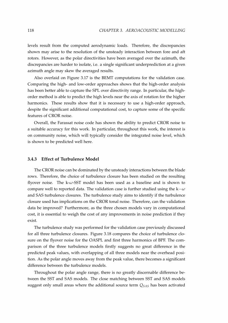
118 CHAPTER 3. AEROACOUSTIC MODELLING
levels result from the computed aerodynamic loads. Therefore, the discrepanciesshown may arise to the resolution of the unsteady interaction between fore and aftrotors. However, as the polar directivities have been averaged over the azimuth, thediscrepancies are harder to isolate, i.e. a single significant underprediction at a givenazimuth angle may skew the averaged results.
Also overlaid on Figure 3.17 is the BEMT computations for the validation case.Comparing the high- and low-order approaches shows that the high-order analysishas been better able to capture the SPL over directivity range. In particular, the high-order method is able to predict the high levels near the axis of rotation for the higherharmonics. These results show that it is necessary to use a high-order approach,despite the significant additional computational cost, to capture some of the specificfeatures of CROR noise.
Overall, the Farassat noise code has shown the ability to predict CROR noise toa suitable accuracy for this work. In particular, throughout this work, the interest ison community noise, which will typically consider the integrated noise level, whichis shown to be predicted well here.
3.4.3 Effect of Turbulence Model
The CROR noise can be dominated by the unsteady interactions between the bladerows. Therefore, the choice of turbulence closure has been studied on the resultingflyover noise. The k-ω-SST model has been used as a baseline and is shown tocompare well to reported data. The validation case is further studied using the k−ω
and SAS turbulence closures. The turbulence study aims to identify if the turbulenceclosure used has implications on the CROR tonal noise. Therefore, can the validationdata be improved? Furthermore, as the three chosen models vary in computationalcost, it is essential to weigh the cost of any improvements in noise prediction if theyexist.
The turbulence study was performed for the validation case previously discussedfor all three turbulence closures. Figure 3.18 compares the choice of turbulence clo-sure on the flyover noise for the OASPL and first three harmonics of BPF. The com-parison of the three turbulence models firstly suggests no great difference in thepredicted peak values, with overlapping of all three models near the overhead posi-tion. As the polar angle moves away from the peak value, there becomes a significantdifference between the turbulence models.
Throughout the polar angle range, there is no greatly discernable difference be-tween the SST and SAS models. The close matching between SST and SAS modelssuggest only small areas where the additional source term QSAS has been activated

3.4. HIGH-ORDER NOISE MODELLING 119
within the SAS model. The k-ω model shows the greatest difference. The most sig-nificant difference is observed near the axis of rotation. This area is dominated by theinteraction between fore and aft rotors and suggests an increased prediction in theunsteady loading components using the k-ω model.
Comparing the trends of the k-ω with the reported data suggests an even greaterdiscrepancy than the SST for the OASPL and first two harmonics of BPF. The k-ωmodel does, however, show improvements for the third harmonic. As a result ofthe improved prediction of the OASPL using the SST model and the reduced costin comparison to the SAS model, the SST turbulence closure is used throughoutthis work in the analysis of CROR noise. In this work, the emphasis is placed oncommunity noise and, therefore, if the interest should be shifted towards a specificnoise component, the turbulence should again be studied to understand its effects onthe resulting source of interest.
Polar Angle, θ [deg]
OA
SP
L [
dB
]
50 100 150
100
110
120
kωSSTSAS
(a) OASPL
Polar Angle, θ [deg]
SP
L [
dB
]
50 100 150
100
110
120kωSSTSAS
(b) BPF1
Polar Angle, θ [deg]
SP
L [
dB
]
50 100 150
100
110
120kωSSTSAS
(c) BPF2
Polar Angle, θ [deg]
SP
L [
dB
]
50 100 150
100
110
120kωSSTSAS
(d) BPF3
Figure 3.18: Effect of turbulence closure on CROR flyover noise for the noise validation case.

120 CHAPTER 3. AEROACOUSTIC MODELLING
3.5 Summary
In this chapter, both low- and high-order methods for the computation of CRORnoise has been presented. Both models were compared against experimental data forCROR noise and showed sufficient agreement to use them for future analysis. Whilstthe low-order model is perhaps only suitable for comparing overall sound levels, itslow computation time makes it ideal as a preliminary design tool. On the other hand,the high-order tool allows for a more in-depth analysis of the noise sources. However,this comes at the cost of a considerably higher computational cost.

Chapter 4
A Parametric Study of CROR Noise
The renewed interest in CROR for next-generation aircraft, in addition to therapid expanse of eVTOL concepts utilising CROR configurations, demands designtools that can accommodate new configurations and large design spaces. In order tomeet this demand, an objective of the present work is to develop a multi-disciplinaryCROR design tool. To accommodate the large design space and the need to evaluatemany design configurations, low-order models have been utilised. In this chapter,the low-order models that have been previously discussed are coupled to develop apreliminary CROR design and analysis tool.
One of the concerns surrounding the integration of CROR configurations is theirnoise emissions. Therefore, design choices for future configurations must focus onnoise reductions and the parameters that affect this. Furthermore, efficiencies in anumber of areas may have to be sacrificed to accommodate reductions in noise. Tothis end, this chapter will first present a parametric study of the two major designfeatures controlling the noise emissions — the blade count and the rotational speed.Following this, the low-order models are coupled to an optimisation routine to de-velop the design tool. Whilst the parametric study has been carried out for a civilaviation sized aircraft, designs are studied for both general and civil aviation classaircraft.
4.1 Blade Count Investigation
The rotor blade count is a significant design choice. Whilst from a performanceand structural perspective, it determines the loading required by each blade to de-liver the total thrust, the choice of blade count also has a significant impact on theresulting noise emissions. Relative to the SRP the additional blade row of the CRORfurther complicates the design process as fore and aft blade count directly affect the
121

122 CHAPTER 4. A PARAMETRIC STUDY OF CROR NOISE
aerodynamic and acoustic interactions. Due to these further complications, the ef-fect of blade count is studied on the resulting CROR noise emissions for a simulatedflyover.
Changes in rotor blade count will affect both the thickness and loading sourcesas both rotor volume and blade loading change. Therefore, to isolate the effectsof differing blade counts, the solidity, σ = Nc/2πR, is held constant. The solidityis maintained by scaling the blade chord and maintaining the spacing-chord ratio.This constraint ensures that the required loading per blade unit area is constant (i.e.
QNA = const.) for all cases and the changes in noise due to blade count result fromacoustic criteria only.
Table 4.1 shows the rotor design parameters used throughout the analysis. TheSR2 geometry [107] was used for all cases. The analysis is carried for civil aviationclass aircraft, which typically utilise large blade count designs [7]. As a result, thedesign values were chosen to be representative of this size of aircraft [52, 72].
Table 4.1: CROR design parameters for parametric noise study.
Parameter σ R1 = R2 [m] g/DValue 0.37 2.13 0.25
The analysis was carried out at take-off, climb-out and approach conditions.These are the most critical phases of flight for aircraft noise evaluation. Table 4.2shows the open rotor operating characteristics at each of these flight conditions. Thetip speed of both rotors are equal at Mt = 0.6, and for each case, the rotors weretrimmed to deliver the same torque. For each case, there is, therefore, a difference indelivered thrust. However, designing for a given torque ratio allows for an appropri-ate design of the gearbox or power turbine to deliver the required torque ratio.
Table 4.2: Operating point parameters.
Operating point Take-off Climb-out ApproachAltitude [feet] 1,000 1,000 1,000Mach Number 0.2 0.3 0.3
CQ/σ 1.02 1.08 0.467
Due to the highly directive nature of CROR noise and in line with civil aviationnoise certification [151], the EPNL metric was used to characterise the CROR noisefor the analysis. A flyover was simulated by placing an array of microphones 1,000 ft(304.8 m) below the CROR to compute the EPNL. The CROR was considered in axialflight throughout the analysis.

4.1. BLADE COUNT INVESTIGATION 123
For the investigation of blade count, a number of fore and aft blade count com-binations are considered. In particular, fore blade counts from eight to fourteen, i.e.N1 ∈Z | 8≤ N1 ≤ 14 and aft blade counts of N2 = N1± 3 are studied. In the analy-sis, cases with equal blade counts are not considered as these are known to generatehigh noise levels due to the simultaneous blade passages [2]. Hence, for the bladecount study, 42 blade count combinations for each operating point are studied.
Due to the large number of blade count configurations studied, only those pro-ducing the lowest and highest EPNL values are presented. Figure 4.1 shows the tencombinations producing the lowest EPNL for all three operating conditions, whilstFigure 4.2 shows those producing the ten highest EPNL values.
N1xN2
EP
NL
[d
B]
12x1
5
12x1
3
12x1
4
12x1
1
11x1
2
10x1
1
11x1
3
11x1
0
10x1
3
11x1
4
45 45
50 50
55 55
60 60
65 65
70 70
(a) Take-offN1xN2
EP
NL
[d
B]
12x1
5
12x1
3
12x1
4
12x1
1
11x1
2
10x1
1
11x1
3
11x1
0
10x1
3
11x1
4
45 45
50 50
55 55
60 60
65 65
70 70
(b) Climb
N1xN2
EP
NL
[d
B]
12x1
3
12x1
5
12x1
4
11x1
2
12x1
1
11x1
3
10x1
1
11x1
4
10x1
3
11x1
0
45 45
50 50
55 55
60 60
65 65
70 70
(c) Approach
Figure 4.1: Blade counts giving lowest EPNL for all operating points.
Figure 4.1 shows that combinations with the highest blade counts produce thelowest computed noise. Conversely, Figure 4.2 shows that the greatest noise is pro-duced by combinations with the lowest blade counts. This trend is in line with thetrends observed by Parry & Vianello [2]. At take-off conditions, there is a differenceof ∼ 35 EPNLdB between the lowest and highest computed blade count combina-tions, illustrating the significant impact blade count has. Recall, the present analysisis from acoustic criteria only and other performance measures would be consideredin the design process.
Comparing the effects of operating point in both Figures 4.1 and 4.2, shows thatthe trend are generally comparable across all operating points. This similarity results

124 CHAPTER 4. A PARAMETRIC STUDY OF CROR NOISE
from the importance of the loading source across all three operating points.
Figures 4.1 and 4.2 also show there is not a consistent increase or decrease innoise with blade count, i.e. at take-off while the 8× 5 produces the highest EPNL,the 10× 7 produces the second-highest, not the 8× 6 as would be expected. Thisresults from the complex interactions between the blade row, i.e. both potential andwake interactions. This illustrates the significance of accounting for the interactioncomponent. Furthermore, it highlights the importance of studying the effect of bladecount for CROR. For SRP, the results would be obvious, with CROR, the interactionadds an additional layer of complexity.
Whilst high blade counts result in low noise, the use of a large number of bladeshas to be weighed against practical issues such as installation as well as ensuringsuitable aerodynamic performance.
N1xN2
EP
NL
[d
B]
8x5
10x7
9x6
8x6
9x7
8x7
8x1
1
9x1
2
11x8
8x1
0
65 65
70 70
75 75
80 80
85 85
90 90
(a) Take-off
N1xN2
EP
NL
[d
B]
8x5
10x7
8x6
9x6
9x7
8x7
8x1
1
11x8
9x1
2
12x9
65 65
70 70
75 75
80 80
85 85
90 90
(b) Climb
N1xN2
EP
NL
[d
B]
8x5
8x6
10x7
9x6
9x7
8x7
8x1
1
8x1
0
11x8
10x8
65 65
70 70
75 75
80 80
85 85
90 90
(c) Approach
Figure 4.2: Blade counts giving highest EPNL for all operating points.
4.2 Tip Speed Investigation
Similarly to the blade count, the rotor tip speed is a critical rotor design choice.The tip speed has a significant effect on a number of CROR parameters, includingthe rotor loading, rotor stress, and importantly the resulting noise. Again, the use

4.2. TIP SPEED INVESTIGATION 125
of two rotors further complicates the design choice. As a result, fore and aft tipspeed combinations are investigated. Tip speed combinations are first studied for thecombination producing the greatest EPNL, namely the 8× 5 configuration.
Tip Mach number combinations between 0.5-0.7 are investigated for each rotor,for take-off, climb-out and approach conditions (Table 4.2). The CROR parameters inTable 4.1 are again used throughout the analysis.
Mt1xMt2
EP
NL
[d
B]
0.5
x0.5
0.5
x0.6
0.5
x0.7
0.6
x0.5
0.6
x0.6
0.6
x0.7
0.7
x0.5
0.7
x0.6
0.7
x0.7
65 65
70 70
75 75
80 80
85 85
90 90
(a) Take-off
Mt1xMt2
EP
NL
[d
B]
0.5
x0.5
0.5
x0.6
0.5
x0.7
0.6
x0.5
0.6
x0.6
0.6
x0.7
0.7
x0.5
0.7
x0.6
0.7
x0.7
65 65
70 70
75 75
80 80
85 85
90 90
(b) Climb
Mt1xMt2
EP
NL
[d
B]
0.5
x0.5
0.5
x0.6
0.5
x0.7
0.6
x0.5
0.6
x0.6
0.6
x0.7
0.7
x0.5
0.7
x0.6
0.7
x0.7
65 65
70 70
75 75
80 80
85 85
90 90
(c) Approach
Figure 4.3: Effect of tip speed on the EPNL of the 8×5 combinations at all operating points.
Fig. 4.3 shows the computed EPNL over the range of tip speeds for each oper-ating point for the 8× 5 combination. The results demonstrate that the computedEPNL generally increases for increasing fore and aft tip speed. The largest EPNLwas computed when Mt1 = Mt2 = 0.7 across all operating points. On the other hand,the lowest EPNL was computed for the tip speed combination, Mt1 = 0.6, Mt2 = 0.5,which is contrary to the expected case of Mt1 = Mt2 = 0.5. However, the differencebetween the two is not significant and results from small differences in the bladeloading∗. Whilst reductions in tip speed are shown to reduce the computed EPNL,this lower limit is constrained by the ability to trim at the given rotational speed.
Comparing the operating point, the trends are comparable across take-off, climb-out and approach conditions. In each configuration, the general trend of increased
∗Small differences in loading are expected between cases as the aerodynamic code trims to therequired loading within a given tolerance.

126 CHAPTER 4. A PARAMETRIC STUDY OF CROR NOISE
noise for increased rotational speed is observed. However, the increase in tip speedappears more sensitive for the aft rotor. This will result from the dominance of theaft rotor due to the interaction component for this case.
4.3 Combined Blade Count and Tip Speed Investigation
The previous two sections have demonstrated that both tip speed and blade counthave a significant effect on the computed CROR noise and, therefore, are importantdesign parameters. As a result, the combined effect of blade count and tip speedon the resulting EPNL is studied. For the analysis, tip speed combinations betweenMach 0.5-0.7 are investigated for various blade count combinations. Due to the largeparameter range, the analysis is carried out for take-off conditions (Table 4.2) only.
Figure 4.4 shows the effect of tip speed with increasing aft blade count. Theresults demonstrate the strong coupling between bade count, tip speed and the com-puted CROR noise. The lowest computed EPNL is found for the lowest tip speedcombination and highest blade count combination.
Mt1xMt2
EP
NL
[d
B]
0.5
x0.5
0.5
x0.6
0.5
x0.7
0.6
x0.5
0.6
x0.6
0.6
x0.7
0.7
x0.5
0.7
x0.6
0.7
x0.7
60 60
65 65
70 70
75 75
80 80
85 85
90 90
(a) N1 = 8, N2 = 9
Mt1xMt2
EP
NL
[d
B]
0.5
x0.5
0.5
x0.6
0.5
x0.7
0.6
x0.5
0.6
x0.6
0.6
x0.7
0.7
x0.5
0.7
x0.6
0.7
x0.7
60 60
65 65
70 70
75 75
80 80
85 85
90 90
(b) N1 = 8, N2 = 10
Mt1xMt2
EP
NL
[d
B]
0.5
x0.5
0.5
x0.6
0.5
x0.7
0.6
x0.5
0.6
x0.6
0.6
x0.7
0.7
x0.5
0.7
x0.6
0.7
x0.7
60 60
65 65
70 70
75 75
80 80
85 85
90 90
(c) N1 = 8, N2 = 11
Figure 4.4: Effect of tip speed with increasing aft blade count.
Figure 4.5 shows the effect of tip speed with increasing fore blade count. Again,the trend of increased EPNL for increasing tip speed is observed. The lowest noise is

4.3. COMBINED BLADE COUNT AND TIP SPEED INVESTIGATION 127
achieved with the lowest tip speeds and greatest blade counts.
Mt1xMt2
EP
NL
[d
B]
0.5
x0.5
0.5
x0.6
0.5
x0.7
0.6
x0.5
0.6
x0.6
0.6
x0.7
0.7
x0.5
0.7
x0.6
0.7
x0.7
60 60
65 65
70 70
75 75
80 80
85 85
90 90
(a) N1 = 9, N2 = 8
Mt1xMt2
EP
NL
[d
B]
0.5
x0.5
0.5
x0.6
0.5
x0.7
0.6
x0.5
0.6
x0.6
0.6
x0.7
0.7
x0.5
0.7
x0.6
0.7
x0.7
60 60
65 65
70 70
75 75
80 80
85 85
90 90
(b) N1 = 10, N2 = 8
Mt1xMt2
EP
NL
[d
B]
0.5
x0.5
0.5
x0.6
0.5
x0.7
0.6
x0.5
0.6
x0.6
0.6
x0.7
0.7
x0.5
0.7
x0.6
0.7
x0.7
60 60
65 65
70 70
75 75
80 80
85 85
90 90
(c) N1 = 11, N2 = 8
Figure 4.5: Effect of tip speed with increasing fore blade count.
Comparing the two cases presented (increasing aft blade count and increasingfore blade count), shows generally that the computed EPNL levels are similar foropposing pairs (e.g. 8× 9,0.5× 0.6 against 9× 8,0.6× 0.5). These comparable levelsshows the importance of both fore and aft rotors to the total noise emissions. Forcomparable blade pairs, the greatest noise is achieved when the rotor with the lowestblade count has the higher tip speed. For example, comparing 8× 9 and 9× 8 con-figurations at Mt1 = 0.5, Mt2 = 0.6, the 9× 8 combination has the highest computedEPNL due to the combination of reduced blade count and increased tip speed. Theresults again show that when the tip speed reaches Mt = 0.7, there is a sharp rise inEPNL for all cases. Whilst the present study has highlighted the complexity of simul-taneously considering the effect of both tip speed and blade count on the resultingCROR noise, the general approach of increasing blade count and reducing tip speedcan be used to reduce noise.
The present study has so far considered only tip speed and blade count. Thestudy highlighted the complex relationship between these two design choices andthe difficulty of comparing designs. Therefore, introducing further design choiceswill only serve to increase the complexity. As a result, a more sophisticated approach
128 CHAPTER 4. A PARAMETRIC STUDY OF CROR NOISE
to considering a greater design space is required.
4.4 Open Rotor Optimisation
4.4.1 Optimisation Routine
Optimisation is the process of finding the set of input parameters (constrainedor unconstrained), that give the best global performance for a given objective (orobjectives). As a design tool, optimisation should allow for an efficient search of thedesign space to locate those parameters that give the greatest performance relative tothe design goal(s) while simultaneously meeting the constraints of the design.
In the context of this work, optimisation has been used to identify CROR geome-tries and configurations that maximise the CROR performance based on a number ofmetrics.
Mathematically, optimisation is the minimisation of a given function. As a result,the earliest optimisation methodologies were gradient-based, e.g. secant method,method of steepest descent, etc. These methodologies are easy to code and computa-tionally inexpensive. However, for large problems, or where the input function is noteasily differentiable, as is the case here, these methods are unsuitable.
Increasing computational power allowed for the development of non-gradientbased methods. For example, Monte Carlo methods. These methods get around theissues of large and complex problems. However, they randomly search the designspace in search of the minima, and can, therefore, be computationally expensive [166].
Population-based optimisation routines are another breed of non-gradient basedmethod. These again can handle large and complex design problems. However, theyuse a defined set of ‘rules’ to drive towards the minima. This approach results inan efficient search for the best performing design. For example, the Particle SwarmOptimisation (PSO) [167] mimics the social behaviour of flocking birds. The particlesfly through the design space while their performance is recorded and updated suchthat all particles follow the paths of the high performing particles. However, if thePSO discovers a local minima, it is typically unable to move from the local to theglobal minima — a disadvantage of this method.
Evolutionary Algorithms form another branch of population-based methods. Inparticular, the Genetic Algorithm mimics the behaviour of natural selection [168, 169].High performing individuals are bred together to successively improve individualsperformance. Due to a number of the GA operations, the global minima may not befound, or it may take some time for it to be bred back into the population. However,the Genetic Algorithm is a robust method that has the ability to handle complex prob-lems, considering a large design space efficiently. To this end, the Genetic Algorithm

4.4. OPEN ROTOR OPTIMISATION 129
was used in the development of the CROR design tool.
The operation of the Genetic Algorithm is presented in Figure 4.6. An initialpopulation of Chromosomes, a data set containing the free parameters (known asPhenotypes), are first generated. The performance (or fitness) of each Chromosomeis evaluated relative to the design goals. Upon evaluation, using processes borrowedfrom evolutionary theory (crossover, mutation, re-insertion), chromosomes are matedto produce a new generation of off-spring. The fittest individuals make it throughsuccessive generations, whilst the least-fit die-off (survival of the fittest). The processis repeated until stopping criteria is met, i.e. the global minimum is found.
Figure 4.6: Operation of a Genetic Algorithm.
Constraint Handling
Every design is subject to constraints. For example, in the present work, thedesign aims to minimise noise. However, this is subject to providing sufficient thrust

130 CHAPTER 4. A PARAMETRIC STUDY OF CROR NOISE
to the aircraft. Also of particular concern is the structural performance of the rotorblade due to design changes. In the present work, a simple beam bending modelis employed to enforce structural constraints [170, 171, 172, 173]. In particular, thecomputed root stress is weighed against material yield stress.
In order to enforce design constraints, penalty functions were utilised. For exam-ple, if a set of input parameters resulted in a design that was particularly close to theyield stress of the material, the design was penalised. This penalty was in the form ofsetting a very low fitness value to ensure it did not progress to the next generation.
Penalty functions were also used to ensure the design stayed within the abilities ofthe models used. For example, designs were not considered when tip Mach numbersexceeded M = 0.75 as no quadrupole noise sources were considered in the noiseanalysis.
Extension to Multiple Objectives
Almost all engineering problems are required to satisfy multiple design goals, e.g.high aerodynamic performance whilst minimising noise. Furthermore, the compet-ing objectives are not necessarily commensurable. Often improvements in one arealead to losses in another. Extending the optimisation to handle multiple objectivesallows for finding a set of solutions that satisfy all design goals without degradingperformance in a single objective.
To handle multiple objectives, the weighted sum approach [174] was used through-out this work. In this approach, objectives are defined within a single objective func-tion and their corresponding performance metrics weighted together to give a singleperformance metric.
The weighted sum approach is easy to implement and computationally efficient [175].The use of the weighted sum approach requires careful consideration of the problemto ensure variables are weighted appropriately. However, this may benefit a designwhere one objective may be valued more than another, so long as the other objectivegives an adequate performance. Additionally, one has to ensure that all objectives aresuitably normalised to ensure slight deviations in a single objective does not domi-nate the overall weighted fitness.
Rotor Geometry Parametrisation
Parametrisation is required to ensure that the spanwise geometry (e.g. chord,twist, etc.), is physically possible, realistic, and to some extent, manufacturable.Parametrisation ensures erratic variations in geometry are not generated and limitsthe number of points of inflexion (changes in directions) of the geometrical propertyalong the span. From an optimisation context, parametrisation is also useful in that it

4.4. OPEN ROTOR OPTIMISATION 131
can significantly reduce the number of free parameters describing the geometry overthe blade span.
The method of Kulfan [176] and Kulfan & Bussoletti [177] was used for parametri-sation of the spanwise varying geometry components. The method proposed uses aclass function/shape function transformation based on Bernstein polynomials to en-sure smooth variations in parametrised geometry. The component shape functiontakes the following form [176]:
Si(ψ) = Ki,nψi(1− ψ)n−i. (4.1)
Where n is the order of the Bernstein polynomial, and i, a counter of this. ψ representsthe area in which the geometrical feature varies (e.g. here, blade span). Ki,n is thebinomial coefficient, given by:
Ki,n =
(ni
)=
n!i!(n− i)!
(4.2)
The individual terms of the Bernstein polynomial are analogous to Pascal’s triangle,as shown in Figure 4.7. For each nth order of Bernstein polynomial, there is n + 1terms required to describe the polynomial. The overall shape function used to repre-sent the geometry component, ζ, at each blade element j, using an nth order Bernsteinpolynomial is then:
Sj = ζmax
n
∑i=0
ζiSi (4.3)
Where ζi ∈ [0 : 1] represents the polynomial values from the optimiser, and ζmax is themaximum value that the geometrical feature can have. Using the chord distributionto illustrate, the blade element chord at each jth blade element using a third-orderBernstein polynomial is then:
cj = cmax
n
∑i=0
ciSi (4.4)
Which upon expansions is:
cj = cmax ·[
c0
( rR
)3+ 3c1
(1− r
R
)( rR
)2+ 3c2
(1− r
R
)2( rR
)+ c3
(1− r
R
)](4.5)
With cmax set by the user and c0 - c3 given by the optimiser, the full spanwise variationof chord can be calculated. This approach reduces the number of free variables fromm spanwise points to only four plus one for the maximum value.
The class/shape function approach allows for a smooth and well-behaved repre-sentation of the spanwise geometry to be quickly and easily generated using only

132 CHAPTER 4. A PARAMETRIC STUDY OF CROR NOISE
a small number of control points. However, using Bernstein polynomials, the con-trol points are evenly spaced along the span. Therefore, this method is not suitablewhere more control would be required in certain areas, e.g. near the location ofpeak loading. This can be overcome using another parametrisation technique, e.g. B-splines. Nonetheless, the present parametrisation is suitable for the present purposesof demonstrating the capability of the optimisation routine.
Figure 4.7: Bernstein polynomial components represented analogously to Pascal’s triangle.
4.4.2 CROR design - Civil Aviation
A Genetic Algorithm optimisation routine [178, 179] was used to perform a pre-liminary design study for a civil aviation class aircraft. Three designs cases wereconsidered, as summarised in Table 4.3. Case I builds on the previous parametricstudy, aiming to find the combination of blade counts and tip speeds that resultin minimum noise. Case II also seeks to find the optimal combination of fore andaft blade count and tips speeds. However, the analysis is extended by consideringthe multiple objectives of minimum take-off noise and maximum cruise efficiency.Case III builds on case I by expanding the design space. The noise was characterisedusing the EPNL metric.
Table 4.3: Optimisation design objectives and free variables
Case Free-variables ObjectiveI N1, N2, Mt1 , Mt2 Take-off NoiseII N1, N2, Mt1 , Mt2 Take-off Noise, cruise efficiencyIII All Take-off Noise
In the analysis of cases I and II, a CROR of 2.125 m fore and aft radius describedby the SR2 geometry [107], Figure 2.8, was used. The upper and lower limits of blade

4.4. OPEN ROTOR OPTIMISATION 133
count and tip speed are presented in Table 4.4Case III considers a greater design space for the minimisation of take-off noise.
In particular, the design space is opened to include tip radius, chord and twist dis-tribution, and axial spacing. The upper and lower limits of the design variables arelisted in Table 4.5. Third-order Bernstein polynomials describe chord and twist dis-tributions. The values presented indicate their minimum and maximum values.
Table 4.4: Upper and lower limits of free variables for optimisation cases I and II.
Variable Lower UpperN1, N2, [−] 8 15Mt1 , Mt2, [−] 0.3 0.6
Table 4.5: Upper and lower limits of free variables for optimisation case III.
Variable Lower UpperN1, N2, [−] 8 15
Mt1 , Mt2 , [−] 0.2 0.6R1 = R2 [m] 1 2.5
c1/R1, c2/R2 [−] 0.25 1.25β1, β2 [] 0 90g/R, [−] 0.25 1
The designs are evaluated at take-off (cases I and III), and take-off and cruise con-ditions (case II). Table 4.6 presents the operating parameters describing the conditionsfor each.
Table 4.6: Take-off and Cruise operating parameters.
Variable Take-off CruiseAltitude [ft] 1,000 36,000
M∞ [-] 0.2 0.7Treq [kN] 80 40
If the population size of the Genetic Algorithm is too small, the design space maynot be fully explored. To this end, the effect of population size on the minimumobjective value was studied for case I. This study should identify the minimum pop-ulation size to obtain an independent solution. A range of population sizes from 10to 500 individuals was studied. Figure 4.8 compares the minimum objective valueobtained across the range of population sizes. Figure 4.8 shows that minimum ob-jective value tends towards a final value as the population size increases. As the
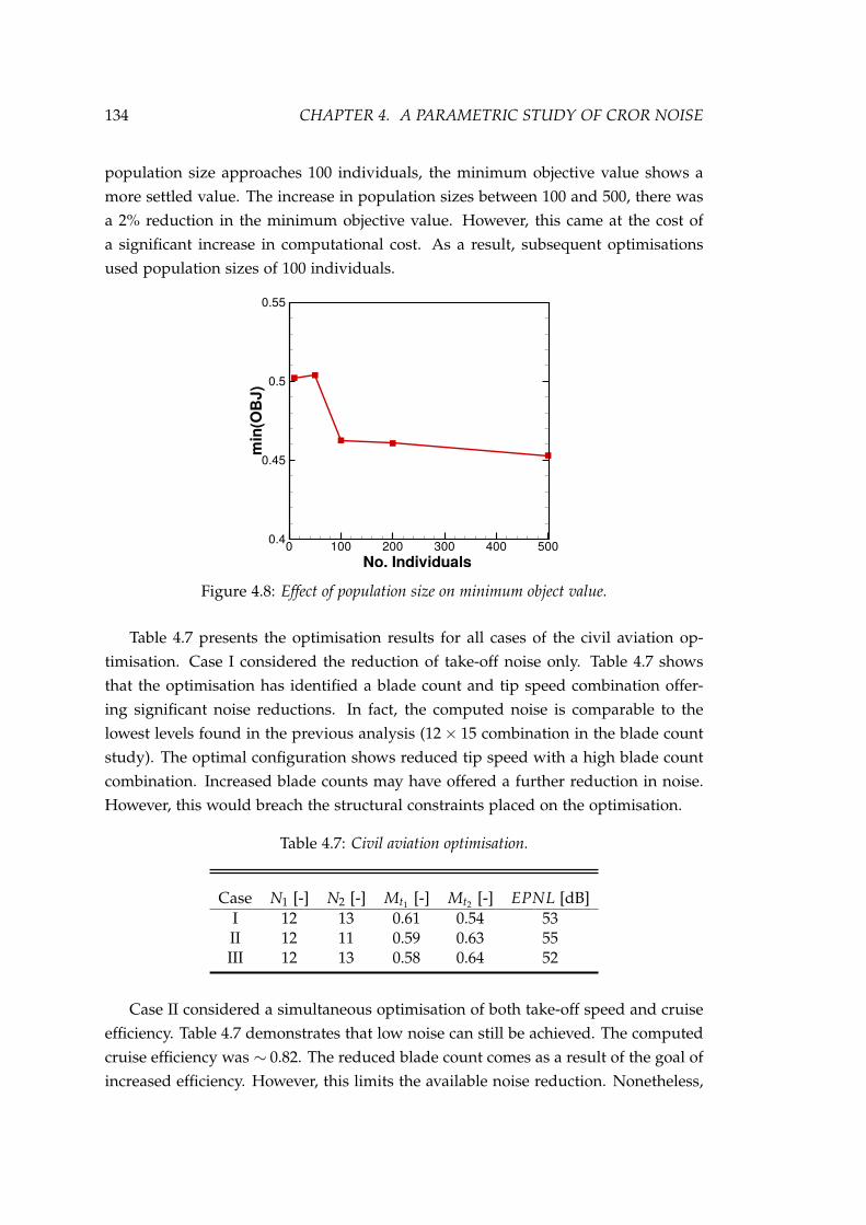
134 CHAPTER 4. A PARAMETRIC STUDY OF CROR NOISE
population size approaches 100 individuals, the minimum objective value shows amore settled value. The increase in population sizes between 100 and 500, there wasa 2% reduction in the minimum objective value. However, this came at the cost ofa significant increase in computational cost. As a result, subsequent optimisationsused population sizes of 100 individuals.
min
(OB
J)
0 100 200 300 400 5000.4
0.45
0.5
0.55
No. Individuals
Figure 4.8: Effect of population size on minimum object value.
Table 4.7 presents the optimisation results for all cases of the civil aviation op-timisation. Case I considered the reduction of take-off noise only. Table 4.7 showsthat the optimisation has identified a blade count and tip speed combination offer-ing significant noise reductions. In fact, the computed noise is comparable to thelowest levels found in the previous analysis (12× 15 combination in the blade countstudy). The optimal configuration shows reduced tip speed with a high blade countcombination. Increased blade counts may have offered a further reduction in noise.However, this would breach the structural constraints placed on the optimisation.
Table 4.7: Civil aviation optimisation.
Case N1 [-] N2 [-] Mt1 [-] Mt2 [-] EPNL [dB]I 12 13 0.61 0.54 53II 12 11 0.59 0.63 55III 12 13 0.58 0.64 52
Case II considered a simultaneous optimisation of both take-off speed and cruiseefficiency. Table 4.7 demonstrates that low noise can still be achieved. The computedcruise efficiency was ∼ 0.82. The reduced blade count comes as a result of the goal ofincreased efficiency. However, this limits the available noise reduction. Nonetheless,

4.4. OPEN ROTOR OPTIMISATION 135
this case demonstrates the potential for CROR design for multiple design goals andconstraints. No sweep was included in the optimisation. However, its inclusionwould be expected to improve the efficiency in cruise through a reduction of therelative Mach number along the span.
Finally, case III builds on case I by expanding the design space, including variationin radius and spanwise geometry. Table 4.7 shows that the increased design space hasallowed for a more significant reduction in noise. It is interesting to note, however,that the same blade count as case I has been retained. On the other hand, there is alarge variation in tip speed, particularly for the aft rotor. Furthermore, the optimiseddesign showed a reduced radius of R1 = R2 = 1.72 m. Again, the optimisation waslimited by the structural constraints imposed.
To explore case III further, Figure 4.9 compares the optimised twist and chorddistributions with the SR2 baseline. Both fore and aft optimised rotors show a reduc-ing chord for increasing radius, as opposed to the almost constant chord (before asudden reduction near the tip) for the baseline SR2 case. The inner rotor section ofthe optimised aft rotor has a reduced chord relative to the fore. However, near thetip area, where loading is greatest, the aft rotor has an increased chord.
r/R []
Ch
ord
(c
/D)
[]
0.4 0.6 0.8 1
0.06
0.08
0.1
0.12
0.14
FOREAFT
SR2Optimised
(a) Chord distribution
r/R []
Tw
ist
[d
eg
]
0.4 0.6 0.8 15
0
5
10
15
20
25
30
35
SR2ForeAft
(b) Twist distribution
Figure 4.9: Spanwise geometry of optimised civil aviation designs.
Comparing the twist distributions, both optimised and baseline distributionsshow similar trends. However, the optimised designs show a reduced twist overmost of the span. As a result, an increased setting angle is required to maintain load-ing, with the chord and twist distributions giving a more optimal loading distribution

136 CHAPTER 4. A PARAMETRIC STUDY OF CROR NOISE
along the span.
To illustrate the designs obtained for each case, Figure 4.10 presents CAD repre-sentations for each optimisation case.
(a) Case I (b) Case II
(c) Case III
Figure 4.10: CAD representations of the optimised civil aviation designs.
4.4.3 CROR design - General Aviation
In line with the current work, a design study has also been carried out for ageneral aviation class aircraft. Following a similar route to the civil aviation design,three cases are again considered, Table 4.3. However, the design variables have beenadjusted for the general aviation case. Furthermore, the LAmax metric is now used tocharacterise the noise of each design. Table 4.8 details the upper and lower limits of

4.4. OPEN ROTOR OPTIMISATION 137
blade count and tip speed for cases I and II. Meanwhile, Table 4.9 details the lowerand upper limits for design variable for case III.
Table 4.8: Upper and lower limits of free variables for optimisation cases I and II.
Variable Lower UpperN1, N2, [−] 3 7Mt1 , Mt2, [−] 0.3 0.6
Table 4.9: Upper and lower limits of free variables for optimisation case III.
Variable Lower UpperN1, N2, [−] 3 7
Mt1 , Mt2 , [−] 0.2 0.6R1 = R2 [m] 0.75 2
c1/R1, c2/R2 [−] 0.25 1.25β1, β2 [] 0 90g/R, [−] 0.25 1
The operating parameters for take-off and cruise also differ for the general avia-tion case. Table 4.10 details the operating parameters for the general aviation analysis.
Table 4.10: Take-off and cruise operating parameters.
Variable Take-off CruiseAltitude [ft] 1,000 25,000
M∞ 0.2 0.45Treq [kN] 6 3
In order to better quantify the optimised designs they are compared against abaseline design. A 4× 4 CROR of 1.5 m radius with Mt1 = Mt2 = 0.46 of SR2 designis used here as the baseline design. The baseline design was computed to have a take-off noise of LAmax = 56.4 dB(A) and cruise efficiency of ηcruise = 0.84 [-]. Table 4.11presents the resulting designs for the three optimisation cases considered.
All three optimisation cases demonstrate reduced take-off noise levels relative tothe baseline configuration. Furthermore, the cruise efficiency of case II shows im-proved levels relative to the baseline. Relative to the civil aviation case noise reduc-tions are more substantial. The high thrust loading of the civil aviation case provedto be quite demanding and is thought to be the reason for the difference in noisereduction relative to the general aviation case.

138 CHAPTER 4. A PARAMETRIC STUDY OF CROR NOISE
Table 4.11: General aviation optimisation.
Case N1 [-] N2 [-] Mt1 [-] Mt2 [-] LAmax [dB] ηcruise [-]I 6 5 0.383 0.355 46.3 -II 4 3 0.437 0.434 50.7 0.856III 7 4 0.299 0.329 42.8 -
For case I, a noise reduction of∼ 10dB(A) has been achieved with high fore and aftblade counts and reduced tip speeds, as demonstrated by the parametric study. Thefore rotor has an increased blade count relative to the aft rotor. The increased bladecount serves to reduce blade loading and reduce interaction and hence noise sourceon the aft rotor. Further noise reduction may be achieved with increased blade countsand reduced tip speeds. However, this is constrained by the structural requirementsimposed on the design. Whilst the additional weight and mechanical complexityof high blade counts were not considered here, they may play an important role inresulting designs.
For case II, the optimisation routine has identified a design that has simultane-ously reduced noise at take-off and improved cruise efficiency. Efficiency gains of∼ 1.6% were observed compared to the baseline. This result was achieved with areduced blade count. However, this reduced blade count has limited noise reduc-tion in comparison with a design for noise only. Along the Pareto front, designswith reduced noise or increased efficiency were observed. However, the identifieddesign had the lowest weighted objective value. This optimisation case highlights thecompeting objectives of CROR noise and efficiency.
A noise reduction at take-off is also achieved for case III with increased bladecount and reduced tip speed. The increase in design space has allowed for an in-creased fore blade count and further reduced tip speed to be achieved before meetingthe design constraints. Opening up the design space has offered an ∼ 13.6 dB noisereduction relative to the baseline configuration and offers the greatest reduction ofall configurations.
Figure 4.11 compares the spanwise geometry of the baseline SR2 and optimisedcase III design. Immediately obvious is the large chord on the optimised aft rotor,resulting from the reduced blade count. Otherwise, the general shape is comparableto the SR2 baseline. Similarly, the twist distribution for the optimised case is fairlysimilar to the SR2 for both fore and aft rotor, with the exception of an increased twistnear the root.
To illustrate the results from the optimisation design study, Figure 4.12 presentsa CAD representation of the computed designs for each optimisation case.

4.5. SUMMARY 139
r/R []
Ch
ord
[m
]
0.4 0.6 0.8 10
0.05
0.1
0.15
0.2
0.25
0.3
0.35
0.4
0.45
0.5
Fore optAft optSR2
(a) Chord distribution
r/R []
Tw
ist
[de
g]
0.2 0.4 0.6 0.8 110
0
10
20
30
Fore optAft optSR2
(b) Twist distribution
Figure 4.11: Spanwise geometry of optimised general aviation designs.
Low-order design tools have been coupled to an optimisation routine to investi-gate low-noise CROR designs for both civil and general aviation class aircraft. Thedesign tool successfully identified low-noise designs. A structural model was usedto apply design constraints and was found to limit the available noise reductions.A multiobjective design for low noise and high efficiency identified the competingnature of both objectives. However, designs must be further evaluated over the rangeof aircraft flight envelope to ensure it can deliver the required thrust and satisfactoryperformance for the range of operating conditions. These additional constraints canbe added into the optimisation routine or tested separately. Overall, optimisationis a useful design tool able to account for various design constraints and objectives.Furthermore, optimisation has met the objective of reducing CROR noise.
4.5 Summary
This chapter has presented a parametric study of CROR noise. The parametricstudy has identified that low-noise can be achieved through high blade counts andlow tip speeds. However, the study also identified a more complex relation whensimultaneously considering both tip speed and blade count. This complexity is com-pounded for CROR due to the additional blade row. As a result of this complexrelation, an optimisation routine has been coupled to the low-order models to de-velop a design tool to perform a design study of low-noise CROR. Carrying out

140 CHAPTER 4. A PARAMETRIC STUDY OF CROR NOISE
design studies of both civil and general aviation class aircraft resulted in reducednoise designs. These designs featured large blade counts and reduced tip speeds.However, further noise reductions were constrained by the structural requirements.A multi-objective optimisation highlighted that low-noise and high cruise efficiencyas competing objectives.
(a) Case I (b) Case II
(c) Case III
Figure 4.12: CAD representations of optimised general aviation CROR.

Chapter 5
CROR Noise Reduction —Low-Order Analysis∗
Whilst CROR can offer significant efficiency savings over conventional propulsionsystems, there are concerns surrounding their noise emissions. These concerns maybe addressed by studying novel concepts aimed at reducing CROR noise. However,to retain viability, these noise reductions must not significantly impact the cruiseefficiency of the CROR. In this chapter, the low-order design tools developed withinthis work are used to investigate a number of novel CROR configurations aimedat reducing noise. Whilst low-order models may not be suitable for detailed andhigh accuracy design, they provide a suitable platform for investigating the effectsof different designs and configurations. Furthermore, the use of low-order modelsallows for a large design space to be considered over a wide operating range. Thischapter investigates a large number of blade count configurations to demonstratepreliminary viability of a number of concepts.
5.1 Description of Proposed Configurations
The novel configurations that have been proposed focus on a variable configura-tion CROR where a single blade row is locked, with the operative rotor providingthe required thrust for the given aircraft manoeuvre. It is proposed to operate witha locked blade row during take-off, climb-out and approach conditions to reduceCROR community noise. Both rotors are operated at their design point during cruiseto retain the high CROR efficiency.
As detailed in Figure 5.1, the analysis considers the following configurations:
∗The work presented in this chapter is published in: D. A. Smith et al. “Noise Reduction of a CounterRotating Open Rotor Through a Locked Blade Row”, Aerospace Science and Technology, 98, 105637, 2020
141
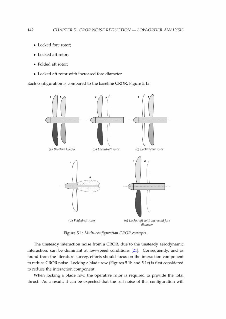
142 CHAPTER 5. CROR NOISE REDUCTION — LOW-ORDER ANALYSIS
• Locked fore rotor;
• Locked aft rotor;
• Folded aft rotor;
• Locked aft rotor with increased fore diameter.
Each configuration is compared to the baseline CROR, Figure 5.1a.
F A
(a) Baseline CROR
F A
(b) Locked-aft rotor
F A
(c) Locked-fore rotor
F
A
(d) Folded-aft rotor
F A
(e) Locked-aft with increased forediameter
Figure 5.1: Multi-configuration CROR concepts.
The unsteady interaction noise from a CROR, due to the unsteady aerodynamicinteraction, can be dominant at low-speed conditions [21]. Consequently, and asfound from the literature survey, efforts should focus on the interaction componentto reduce CROR noise. Locking a blade row (Figures 5.1b and 5.1c) is first consideredto reduce the interaction component.
When locking a blade row, the operative rotor is required to provide the totalthrust. As a result, it can be expected that the self-noise of this configuration will

5.1. DESCRIPTION OF PROPOSED CONFIGURATIONS 143
increase. When locking a blade row, there will still exist an unsteady interactioncomponent of the noise. However, this will be weaker than the fully operative CRORconfiguration. Therefore, to prove the viability of the locked row configurations, thereduction in the interaction component must reduce sufficiently to negate the increasein self-noise.
In an attempt to further reduce interaction noise, the locked-aft rotor is foldedbackwards, Figure 5.1d. Whilst there will again be an increase in the self-noise, theinteraction component should now be eliminated. During cruise, the aft rotor isunfolded and operated at design conditions. The folding is controlled by a joint atthe blade root. The folding rotor is only considered from an acoustic point of view,and detailed mechanical design is not undertaken. This is justified as there are anumber of works considering a folding rotor for distributed propulsion concepts,e.g. see Refs. [180, 181]. The folded rotor concept will have a behaviour similar tothat of the SRP. As a result, it is modelled as such throughout the analysis.
The noise gains of the locked rotor concepts are limited by the increase in self-noise as the operative rotor takes on the full thrust requirements. The effect of in-creasing fore radius with a locked aft rotor is studied to investigate the possible noisereduction of unloading the operative rotor. For increasing fore radius, tip speed ismaintained by reducing the rotational speed.
In order to investigate the noise-reducing capabilities of the outlined concepts, athorough analysis considering a large design and operating space must be consid-ered. The use of low-order models affords such an exhaustive analysis which wouldbe otherwise unaffordable with other numerical tools. The analysis is considered forthe terminal areas, namely take-off, climb-out and approach conditions. Table 5.1presents the details of these flight conditions. The values shown were computed forthe Beechcraft 350i aircraft using the FLIGHT aircraft performance software [147, 182]to represent a general aviation class aircraft for which the analysis was performed.
Table 5.1: Operating point parameters.
Operating point Take-off Climb ApproachAltitude [ft] 1,000 1,000 1,000
Mx [-] 0.2 0.3 0.3CT [-] 0.30 0.19 0.092
The aerodynamic performance and the resulting noise was computed for a rangeof blade count configurations from 4 to 6 on the fore rotor and 3 to 7 on the aft rotor.These blade count combinations were chosen as representative of modern propeller-driven general aviation aircraft. To isolate the effects of increasing blade count and toensure a physical geometry as the blade count increases, the blade chord is scaled to

144 CHAPTER 5. CROR NOISE REDUCTION — LOW-ORDER ANALYSIS
ensure constant solidity. Therefore, the differences in computed noise level are fromacoustic criteria only.
The viability of each concept is determined based on comparisons of computednoise against the baseline configuration. In line with general aviation certification,the maximum A-weighted SPL (LAmax) noise metric is used throughout the analy-sis [149]. Certification procedures require a single microphone measurement at thesecond segment of take-off. The aircraft altitude at which the measurement is taken isdependent on the aircraft performance. Therefore, to generalise and to allow for com-parisons with climb-out and approach segments, a constant 1,000 ft (304.8m) flyoveris simulated. Furthermore, a constant flyover allows for the CROR to be consideredin steady level flight.
During the simulated flyover, only CROR sources are considered, i.e. the CRORis in isolation with no other aircraft sources accounted for. Considering the CRORin isolation is required so that the gains or losses of the current concepts can becompared. Furthermore, it is not envisaged that aircraft sources are likely to differbetween installations of the proposed CROR concepts.
Following the operating requirements outlined in Table 5.1, a generic tractorCROR has been designed for the analysis. The CROR utilises the SR2 geometry [107],Figure 2.8. Further rotor design parameters are presented in Table 5.2. Clippingof the aft rotor is typically employed in CROR to minimise tip vortex interactionnoise [32, 37]. However, in order to compare both fore-locked and aft-locked rotors,no clipping has been employed. For example, a clipped aft rotor may have an in-creased loading and therefore, would be disadvantaged when comparing to the forerotor with reduced loading. Future designs using a locked-rotor configuration maybe optimised to reduce tip vortex interaction noise through clipping.
Table 5.2: Rotor design parameters.
Parameter σ R1 = R2 [m] rh/R g/R MTValue 0.36 1.5 0.24 0.4 0.46
5.2 Locked-Fore Rotor
The locked-fore configuration is first considered. In the locked-fore configura-tion, the fore rotor is locked and trimmed to minimise torque, while the aft rotoris trimmed to deliver the thrust required by the aircraft plus that to overcome thecomputed drag of the locked row. The primary noise source from this configurationwill be the self-noise of the baseline rotor and the interaction noise of the aft rotoroperating in the wake and potential field of the locked-fore rotor.

5.2. LOCKED-FORE ROTOR 145
Figure 5.2 compares the computed LAmax for each blade count combination ateach operating point calculated for the operative baseline and locked-fore configura-tions. Despite differences in absolute level, Figure 5.2 shows that the computed trendsfor each blade count combination are consistent across all three operating conditions.These comparable trends result from the dominance of the loading source at theseparticular conditions. It is understood during approach conditions that other aircraftnoise sources may dominate the emitted sound field. However, this is not consideredhere as the interest is purely in comparing the different CROR configurations.
(a) Take-off (b) Climb-out
(c) Approach
Figure 5.2: Comparison of noise between baseline CROR and a CROR with locked-foreblade row. CROR is the baseline configuration and inop the locked-rotor configuration.
To proceed with a discussion of the results, it is worthwhile to briefly describethe noise sources and what is being compared. CROR noise is known to be highlydirective; typical flyovers are characterised by a peak near the rotor plane due to theself-noise and high values near the axis of rotation due to the unsteady interactions.In the analysis, comparisons are made using the LAmax metric. Therefore, compar-isons are likely to be between those values near the rotor plane, i.e. the self-noise.

146 CHAPTER 5. CROR NOISE REDUCTION — LOW-ORDER ANALYSIS
From Equation (3.12), in particular the integral term, the acoustic pressure is pro-portional to the product of some amplitude (the part containing the thickness orloading terms, although the loading will dominate here), and a radiation efficiency(the part containing the Bessel function). For both baseline and inoperative configu-rations, the steady loading source (giving rise to self-noise) will radiate with the sameefficiency (i.e. k1 = 0 for the aft rotor, k2 = 0 for the fore rotor). Furthermore, as thesolidity is held constant for increasing blade counts, the loading per unit blade areawill also remain constant. As a result, for a given configuration, differences in noisewill be from acoustic criteria due to changes in blade count. Differences in noiselevel observed between the two configurations will also arise due to the differencesin loading between the two configurations, i.e. delivered by a single or two bladerows. Differences will also arise due to the specific blade count combination of thebaseline configuration due to acoustic interactions.
The reasoning for the observed differences is evidenced with reference to Fig-ure 5.2. For example, computed noise levels are comparable for equal aft blade counts(the operative row). When considering the baseline configuration, computed noiselevels are observed to be similar between opposite blade pairs, for example, the 5× 4and 4× 5 combinations. This similarity is only valid here as the rotors are equallyloaded and operating at the same rotational speed.
Considering the baseline operative configuration, Figure 5.2 demonstrates a noisereduction for increases in both fore and aft blade counts. The exception to this occursfor equal blade count combinations, where the acoustic interaction (the constructiveaddition of fore and aft signals), results in increased sound level. This agrees with theresults of §4.1. For the locked-fore configuration, it is shown that the computed noisedecreases for increasing aft blade count (i.e. the operative row). Throughout theanalysis, it was observed that the locked rotor produced a negligible contributionto the total noise. The result of equal blade counts is an increased noise of thebaseline configuration over the locked-aft configuration. However, this may resultin unsuitably high levels during cruise and must, therefore, be carefully assessedover the whole flight envelope.
With the exception of the 6× 7 blade count combination, Figure 5.2 shows thatthe locked-fore combination is generally computed to produce less noise than thebaseline configuration when N2 > N1. This reduction is seen to increase as the dif-ference in blade count increases. Investigating the noise sources further, it was foundthat both fore and aft rotors of the baseline configuration produce less noise than thelocked-fore configuration. However, the addition of their pressure signals results ina greater noise level.
With a reduction of around 3 dB(A), the lock-fore configuration with a 4× 6 blade

5.3. LOCKED-AFT ROTOR 147
count showed the greatest reductions against the baseline configuration. However,the 6× 7 baseline configuration showed the lowest computed noise levels across alloperating points. Nonetheless, the fore-locked configuration has demonstrated noisereductions relative to the baseline CROR whilst maintaining the required aircraftthrust. The current case used an unoptimised CROR that has been scaled to ensureequal loading across the blade count investigation. Therefore, an optimised designsized appropriately may offer more significant reductions in noise compared to thosedemonstrated here.
5.3 Locked-Aft Rotor
The locked-aft configuration comprises an operative fore rotor trimmed to deliverthe required thrust and a locked aft rotor trimmed to minimise torque. In this con-figuration, the noise will be dominated by the self-noise of the operative fore rotor.The unsteady potential interactions, resulting in unsteady noise, will also contributeto the total noise. The interaction of the fore wake with the stationary aft row willresult in unsteady noise being produced by the locked row.
Figure 5.3 compares the computed LAmax for baseline and locked-aft CROR con-figurations for the range of blade count combinations over the three operating points.Similarly to the lock-fore analysis, Figure 5.3 demonstrates that the computed trendsare consistent over the three operating conditions. Again, this is due to the dom-inance of the loading source at these particular operating points. Similarly to thelocked-fore study, the approach conditions show the lowest noise levels.
The sources of difference in computed noise level, in this case, will be as de-scribed previously for the locked-fore analysis. Figure 5.3 shows that the computedLAmax is comparable across fore blade counts. These comparable levels result fromthe requirement of constant solidity to ensure differences in noise level arise fromacoustic criteria only. In addition to the effects of blade count, recall that differencesin noise is also due to differences in loading, i.e. load split between one or two bladerows. To this end, the increased noise of the locked-aft configuration when N1 = 4results in greater computed noise than the operative configuration. As the fore bladecount increases, the locked-aft configuration begins to demonstrate noise reductions.Therefore, the locked-aft configuration shows reduced noise compared to the base-line configuration when N2 ≤ N1. In each case, the noise of the individual rotorsof the operative configuration is computed to produce less noise than the locked-aftconfiguration. It is again, the acoustic interaction that results in increased noise lev-els. As the aft blade count increases and N2 > N1 the reduction in noise of the CRORconfiguration is such that the addition of the acoustic pressure of fore and aft rows

148 CHAPTER 5. CROR NOISE REDUCTION — LOW-ORDER ANALYSIS
drops below that of the locked-aft configuration. The analysis found that the lockedrotor of the locked-aft configuration produced a negligible contribution to the totalnoise.
(a) Take-off (b) Climb-out
(c) Approach
Figure 5.3: Comparison of noise between baseline CROR and a CROR with locked-aft bladerow. CROR is the baseline configuration and inop the locked-rotor configuration.
The lowest predicted noise level was again observed for the 6 × 7 case of thebaseline configuration. However, the locked-aft presented a number of blade countsoffering noise reductions. The 5× 3 combination demonstrated the most significantreductions relative to the operative configuration of ∼ 3 dB(A) at take-off. Thesereductions can be further widened by increasing the fore blade count relative to theaft. This is the opposite conclusion found for the locked-fore configuration.
Comparing the locked-fore and locked-aft configurations show that the computednoise of the locked-aft configuration is marginally higher than the locked-fore config-uration. Note, comparisons are made for opposing blade pairs, i.e. 4× 6 comparedwith the 6 × 4 blade count. Under further inspection, this result arises from thecomputed aerodynamic performance. Locking the fore rotor was found to have an

5.3. LOCKED-AFT ROTOR 149
aerodynamic benefit, with the computed induced velocity component lowering theinflow and hence required blade setting angle to deliver the required thrust. On theother hand, the locked-aft rotor did not benefit from the operative rotor, and thereforethe locked-aft configuration had a poorer aerodynamic performance.
In line with general aviation certification [149], the LAmax noise metric has so farbeen used throughout the analysis. However, due to the highly directive nature ofCROR noise, it is perhaps not the most suitable metric in which to compare the var-ious configurations. Due to the properties of the EPNL metric (§3.2), it is perhapsmore suited for the CROR analysis. To this end, using the same constant 1,000 ft(304.8 m) flyover, the EPNL has been computed for operative and locked-row config-urations at the take-off conditions. Figure 5.4 compares the computed EPNL of thebaseline and locked-rotor configurations for the range of blade counts.
(a) Locked-fore (b) Locked-aft
Figure 5.4: EPNL of baseline operative CROR and a CROR with a locked blade row. CRORis the baseline configuration and inop the locked-rotor configuration.
Using the EPNL metric will make isolating the noise differences between configu-rations more difficult. The steady components will again be important. However, theinteraction components are now better represented with the noise metric. The steadytones will again radiate with the same efficiency across configurations. Additionally,there are a number of interaction harmonics that will radiate very efficiently alongthe rotor axis (ν = N1k1 + N2k2 = 0) for all configurations. However, the amplitudeswill differ as the loading changes for each configuration.
Figure 5.4 presents similar trends for both locked-fore and locked-aft configura-tions as when the LAmax metric is used. However, the differences between oper-ative and inoperative configurations now appear wider. Therefore, the use of theEPNL metric has not highlighted further combinations demonstrating noise reduc-tions. However, its use, and hence the inclusion of interaction components (i.e. thosenot near the plane of rotation) result in greater differences between inoperative and

150 CHAPTER 5. CROR NOISE REDUCTION — LOW-ORDER ANALYSIS
baseline configurations. Locking the fore rotor results in a maximum reduction of ∼ 4EPNLdB with a 4× 6 blade count. When the aft row is locked, a maximum reductionof ∼ 6 EPNLdB can be achieved with a 5× 3 blade count. Again, the lowest noise isachieved with the operative configuration utilising 6× 7 blade count.
Whilst locking the aft rotor was found to offer noise reductions for a number ofblade counts, these reductions came at the cost of a ∼ 5% reduction in efficiency. Nev-ertheless, the take-off, climb-out and approach conditions are comparatively shortsegments relative to the cruise segment and, therefore, this penalty may be justifiableas the cruise efficiency is retained when using the proposed concepts.
5.3.1 Folded Aft Rotor
In an effort to further reduce the interaction noise, the effect of folding the locked-aft rotor backwards is studied, Figure 5.1d. In the folded-aft configuration, the aftrotor is locked and folded backwards in the terminal area. In cruise conditions, itis unfolded and operated at the design point. The folded rotor should eliminate theinteraction component of the CROR noise. Furthermore, compared to the locked-aftcase, the inoperative rotor drag is eliminated and hence reduces the loading demandsand the subsequent loading source of the operative fore rotor.
The folded-aft rotor is modelled as an isolated SRP. The SRP is trimmed to deliverthe required thrust and the flyover simulated in order to compute the LAmax. In or-der to evaluate the performance of the folded-aft configuration, Figure 5.5 comparesthe computed LAmax of the locked-aft and folded-aft configurations at take-off condi-tions. Figure 5.5 demonstrates that the folded aft rotor concept is computed to offersignificant noise reductions in comparison to the locked-aft configuration across allblade counts. The reduction in noise results from a number of sources. Firstly, thecontribution of the unsteady interaction between the locked and operative rotor isnot present in the folded configuration. In the unfolded configuration, the presenceof the locked-aft rotor increases the loading demands on the operative rotor. Thisincreased loading arises from the increased drag due to the presence of the aft rotor.Furthermore, it was found that the presence of the locked-aft rotor induced a veloc-ity on the fore rotor such that an increased setting angle was required to achieve thetarget thrust. These additional loading components are eliminated by folding the aftrotor. When N1 = 4, a maximum reduction of ∼ 10 dB(A) was computed when thelocked-aft rotor was folded backwards.

5.3. LOCKED-AFT ROTOR 151
Figure 5.5: Comparison of total noise locked-aft and folded-aft rotors for take-off conditions.
Across all blade counts, significant noise reductions are observed. Comparingthe computed noise of the folded-rotor with the baseline also demonstrates noisereductions across all blade counts. Nonetheless, the additional complexity and massof the folding mechanism must be weighed against the presented benefits. However,as the aft rotor will be used only for cruise, it can be designed independently of anytake-off requirements.
5.3.2 Increased Fore Radius
When either fore or aft rotor is locked, noise reductions are limited by the in-crease in self-noise as the operative rotor now provides the total required thrust.Therefore, to reduce this loading component, the effect of increasing the fore radiusof the locked-aft configuration is studied. For increasing radius, the tip speed ismaintained by reducing the rotational speed. Noise reductions will primarily arisedue to reduced blade element loading and the reduced rotation rate. Furthermore,the increased rotor radius will have a similar effect as clipping the aft rotor radius byreducing the tip vortex interaction with the aft rotor.
The fore rotor radius is increased by a maximum of 30% for the range of fore andaft blade count combinations at the take-off operating point. Figure 5.6 comparesthe computed LAmax for both baseline and aft-locked configurations with increasedfore radius at the take-off operating point. Figure 5.6 demonstrates a computednoise reduction for both configurations relative to no increase in fore tip radius, seeFigure 5.3a.
Considering the baseline configuration, for cases where the aft rotor noise domi-nates, in particular, N2 > N1, the impact of increasing fore tip radius has a negligibleeffect. Comparing the effects of increasing tip radius shows there is not a linear effect

152 CHAPTER 5. CROR NOISE REDUCTION — LOW-ORDER ANALYSIS
on the computed noise for both configurations. This result is believed to arise fromthe trade-off between the reduction in rotational speed to maintain the tip speed andthe resulting required increase in setting angle. Nonetheless, there are a number ofblade counts that demonstrate increased reductions when the fore rotor tip radius isincreased.
As the fore rotor radius increases, there are a number of additional parametersthat further complicate the changes in noise. Firstly, as the tip radius increases, thetorque ratio of the operative configuration will reduce, and this is known to have animportant role on the resulting noise [31]. Additionally, the effect of unloading isexpected to be more significant for the locked-aft configuration. As the fore row ofthe operative configuration produces only half of the required loading, in comparisonto the total loading produced by the operative row of the locked-aft configuration,the operative configuration will be less sensitive to changes in loading.
(a) ∆R1 = 10% (b) ∆R1 = 20%
(c) ∆R1 = 30%
Figure 5.6: Effect of increasing radius on locked-aft and baseline CROR configurations.

5.3. LOCKED-AFT ROTOR 153
The increase in fore radius, nonetheless, offers increased reductions for the locked-aft configuration over the baseline configuration. To further demonstrate this point,Figure 5.7 presents the computed noise reduction of the locked aft configuration with6× 4 blade count over the operative configuration for a range of increasing tip radii.Note that the negative value corresponds to reduced noise relative to the operativeconfiguration. Figure 5.7 demonstrates that a noise reduction of up to ∼ 8 dB(A) canbe achieved with the maximum increased radius of 30%. Additional noise reduc-tions will also result from a reduction in the tip vortex interaction noise as the radiusincreases.
Figure 5.7: Difference in noise between locked-aft and operative CROR for increasing radiusfor the 6× 4 combination.
As the tip radius is increased, the resulting computed propulsive efficiency wasfound to reduce significantly. For a 10% increase in radius, a drop in efficiency of∼ 10% resulted. This efficiency drop results from a move away from the optimal lift-drag ratio as the radius increases and the rotational rate is reduced, the inflow angleto rotor will change. This is an important point, particularly as the aircraft transitionsto cruise. The difference between take-off and cruise design points now widens asthe fore rotor is designed for a much higher loading during take-off compared to itsbaseline configuration counterpart.
Increasing the fore radius was utilised in order to reduce the loading of the op-erative row of the locked-aft configuration. For a number of configurations, thisdemonstrated further reductions than the baseline locked-aft configuration. How-ever, the reduction in noise was also accompanied by a significant drop in propulsiveefficiency. However, it may be possible to alleviate the efficiency reduction by opti-misation of the design. Furthermore, the lowest noise was achieved by an operativeCROR configuration with increased tip radius.
154 CHAPTER 5. CROR NOISE REDUCTION — LOW-ORDER ANALYSIS
5.4 Summary
In this section, low-order models have been used to investigate the noise-reducingpotential of a number of novel CROR configurations. In particular, the concept oflocking a blade row has been studied to reduce CROR interaction noise. The analysisshowed that the concepts could successfully reduce noise for a number of CRORdesigns. A maximum reduction of ∼ 3 dB(A) when either fore or aft rotor is lockedwas observed for take-off conditions. It was also found that further reductions couldbe achieved by folding the aft rotor or increasing the fore rotor radius of the locked-aft concept at selected blade counts. Nonetheless, the lowest noise was observed fora high blade count baseline CROR. However, the use of a high blade count must beweighed against the additional mass and the aerodynamic implications. Therefore,future work should consider an optimisation of the novel CROR configurations ina multidisciplinary approach. Furthermore, the low-order models can only provideindicative results and must be further verified.

Chapter 6
CROR Noise Reduction —High-Order Analysis∗
The previous chapter (§5) indicated that for selected blade counts, CROR noisecould be reduced in the terminal area by locking a blade row. The locked row isoperated at design speed during cruise to retain the high propulsive efficiency of theCROR. The previous analysis highlighted the potential of the locked-rotor conceptutilising low-order models. Therefore, these findings must be further investigatedwith models providing a higher fidelity representation of the physics. The aim ofthis section is then to study the noise-reducing potential of the locked rotor conceptutilising high-order models. Furthermore, the use of high-order models will providea greater description and insight into the noise sources of the locked-rotor concept.
6.1 Description of Test Cases
Four configurations are studied: (i) operative CROR (baseline); (ii) locked-foreCROR; (iii) locked-aft CROR; (iv) an isolated single rotation rotor (SRP). These con-figurations are illustrated in Figure 6.1. The baseline and locked rotor configurationshave N1 = N2 = 4 rotor blades, whilst the SRP has N = 4 rotor blades. The SRP maybe likened to the folded aft rotor studied previously.
All configurations are of SR2 design, Figure 2.8. Pertinent design features areoutlined in Table 6.1. Note: the design differs from the previous low-order analysisas the current rotors do not have to be scaled in order to compare a large variationin blade count. Despite the fact that clipping has been identified as a design solutionto reduce CROR noise (§1.2), it is not utilised here in order to better compare the
∗The work presented in this chapter is published in: D. A. Smith et al. “Acoustic Analysis ofCounter-Rotating Open Rotors with a Locked Blade Row”, AIAA Journal, 2020.
155

156 CHAPTER 6. CROR NOISE REDUCTION — HIGH-ORDER ANALYSIS
configurations. In particular, when comparing locked-fore and locked-aft configura-tions, it is important that the rotors have similar loading such that one configurationis not acoustically biased. This is achieved by utilising the same design for all config-urations. Nonetheless, future designs could utilise clipping to further reduce noise.
Table 6.1: Rotor design parameters.
Parameter R1 = R2 [m] rh/R g/R MTValue 1.5 0.24 0.4 0.46
The analysis was carried out at take-off conditions. In particular, the free-streamMach number was M∞ = 0.2, take-off thrust, T = 6 kN. The configurations weresimulated in steady level flight at an altitude of h = 1,000 ft (304.8 m). These valuesare used to be representative of a general aviation class aircraft.
(a) Operative CROR (b) SRP
(c) Locked-fore CROR (d) Locked-aft CROR
Figure 6.1: Baseline and inoperative configurations.

6.2. AERODYNAMIC ANALYSIS 157
6.2 Aerodynamic Analysis
The HMB solver was used to perform the high-order CFD analysis for each con-figuration. The medium background and Chimera grids described in § 2.2.4 were usedfor each computation. In addition, each simulation utilised the k-ω SST turbulenceclosure. The HMB3 solver adopts a non-dimensional approach. To return to physicalflow properties, a Reynolds number, based on tip chord of Re = 7.34e + 5 was usedto simulate the described take-off properties.
Unsteady simulations, i.e. those for the baseline and locked-rotor configurations,required at least four rotations to give time-invariance of flow variables. A final rev-olution was subsequently computed from which flow variables were extracted. Theunsteady simulations used a time step corresponding to 0.5 for which blade surfacepressure data were extracted. The SRP configuration utilised a steady simulation.Convergence was monitored using a number of metrics. These included trackingresiduals at each time-step and monitoring surface loads and flow variables at eachtime step using numerical probes placed at a number of locations within the flow-field. Convergence was met when loads and flow variables showed a periodic solu-tion. Figure 6.2 demonstrates a number of the convergence monitors for the baselineconfiguration. Namely axial pressure and viscous blade forces, and flowfield densityat a location downstream of the fore rotor. The convergence monitors show that aftersome initial large transient fluctuations, the solution converges to a periodic variationin each variable. There is a slight fluctuation located ∼ 4500 iterations. This changeresults from varying fore and aft rotor setting angles to adjust the thrust closer to thetarget value. Following this sudden fluctuation, the variables quickly returned to aperiodic value.
The flowfield and surface data were extracted over the final rotation for post-processing. The data extracted is used to perform an aerodynamic analysis of eachconfiguration. This analysis compares the aerodynamic performance of each config-uration, allowing for any aerodynamic benefits or penalties to be weighed againstany corresponding changes to the noise with reference to the baseline configuration.The aerodynamic analysis also allows for greater insight into the noise generatingmechanisms that drive the differences in noise between each configuration.
Whilst the locked-rotor concept is concerned with reducing CROR noise, it mustalso provide the required thrust for the aircraft. For the take-off condition consideredhere, the required thrust was computed as T = 6 kN. The initial setting angles foreach configuration were computed using the BEMT aerodynamic tool. The operativeconfiguration was trimmed with an equal thrust split, whilst the SRP configurationand the operative rotor of the locked-rotor configurations were trimmed to deliver thefull required thrust. Table 6.2 details the setting angles used for each configuration.

158 CHAPTER 6. CROR NOISE REDUCTION — HIGH-ORDER ANALYSIS
Iterations []
Cp
x [
]
0 2000 4000 6000
20
0
(a) Axial pressure force
Iterations []
Cτx [
]
0 2000 4000 6000
0
4
(b) Axial visocus force
Iterations []
ρ/ρ
ref [
]
0 2000 4000 60000.98
1
1.02
(c) Normalised density
Figure 6.2: Convergance monitors for CFD simulations (initial transients cropped to showfinal periodicity).
The locked-aft and baseline configurations required slight adjustments during theCFD computations. Table 6.3 presents the computed thrust for each configuration.
All configurations are within 5% of the target thrust. These could be trimmedcloser to the required value with finer adjustment of the setting angle. However, thiswould require significant additional computational cost and withal the current valuesare sufficiently close to compare the aerodynamic and aeroacoustic performance ofeach configuration. For example considering the SRP configuration, using the BEMTtool, a 5% change in thrust resulted in < 0.5 [dB] change in peak noise level.

6.2. AERODYNAMIC ANALYSIS 159
Table 6.2: Fore and aft rotor setting angles for each configuration.
Configuration β1.75 [] β2.75 [
]Baseline 33.0 32.7
Locked-fore 83.2 37.2Locked-aft 36.8 83.4
SRP 37.8 -
Table 6.3: Computed thrust for each configuration. Target thrust = 6 kN.
Case T1[kN] T2 [kN] T1 + T2 [kN] ∆Target [%]Baseline 3.05 3.06 6.11 +1.89
Locked-fore −0.145 6.34 6.14 +2.37Locked-aft 5.94 −0.01 5.85 −2.56
SRP 6.30 - 6.30 +4.83
Table 6.3 shows that the baseline configuration has an almost equal thrust ratio,i.e. T2
T1∼ 1. Considering the locked-rotor configurations, the operative rotors have all
shown the capability to provide the required thrust for the aircraft. Concurrently, thelocked rotor for all configurations produces minimal levels of negative thrust.
Whereas the operative rotor of the locked-rotor configurations was trimmed todeliver the total thrust, the locked rotor was trimmed to minimise torque. Table 6.4presents the computed torque for each configuration. The baseline configurationshows a torque ratio of almost unity, i.e. Q2
Q1∼ 1. Although the design was for
equal thrust, the equal torque will result from a high efficiency of the configuration.The locked rotor of the locked-fore configuration has been successfully trimmed toa sufficiently small value. On the other hand, the locked rotor of the locked-aft con-figuration produces a significant torque value. This torque results from the inducedswirl from the fore rotor impacting on the aft rotor. Therefore, this indicates thatthe BEMT model has underpredicted this component. This torque may be reducedby adjusting the rotor setting angle. However, this torque reduction will have to beweighed against resulting negative thrust.
The operative rotors of all locked-row configurations, in addition to the SRP con-figuration, produce a torque of similar magnitude to the absolute sum of both base-line rotors. Despite this high torque reaction, the value is well within the limits of theengine†.
†The torque reaction is within the limits of the engine used by the aircraft modelled to obtain thethrust requirements.

160 CHAPTER 6. CROR NOISE REDUCTION — HIGH-ORDER ANALYSIS
Table 6.4: Computed torque and efficiency of each configuration.
Case Q1 [kNm] Q2 [kNm] η [-]Baseline −2.50 2.49 0.794
Locked-fore 0.233 5.55 0.739Locked-aft −5.22 1.55 0.737
SRP −5.44 - 0.750
Table 6.4 also shows the computed efficiency, where the efficiency was computedaccording to:
η =V∞ (T1 + T2)
Ω1Q1 + Ω2Q2. (6.1)
The baseline configuration is shown to have the highest efficiency of all configu-rations. The locked-rotor configurations show a reduced efficiency relative to thebaseline.
One source of improved efficiency of the CROR arises due to the counter-rotationof the aft rotor as the angular momentum from the fore rotor is transformed intouseful axial momentum. In particular, the counter-rotation of the aft rotor inducesa tangential velocity in the opposite sense from the fore rotor, resulting in a partialcancellation of the tangential velocity downstream. Figure 6.3 shows the computedtime-averaged normalised tangential velocity far downstream of all configurations.The baseline configuration is shown to result in an almost complete cancellation ofthe downstream tangential component. This cancellation is in contrast to all otherconfigurations which show significant downstream tangential components.
Locked-fore and locked-aft configurations have downstream components oppo-site in direction due to the opposing sense of their operative rotors. Consideringthe locked-aft configuration, the induced tangential component from the fore rotorwill pass over the stationary aft row, and this interaction is seen to impact the result-ing downstream profile. The reduction of the tangential component in the inboardsections demonstrates that the aft rotor may be adjusted to act as an outlet guidevane and reduce the tangential component further. Conversely, the fore rotor of thelocked-fore configurations may be used as an inlet guide vane. However, these con-figurations would require some further study.
The mutual interactions between CROR blade rows result in unsteady loadingand hence, an unsteady acoustic sources across both rotors. Figure 6.4 presents thecomputed axial force produced by each operative blade row over a single rotation forbaseline and locked-row configurations.

6.2. AERODYNAMIC ANALYSIS 161
V/Vref
[]
r/R
[]
0.2 0.1 0 0.1 0.2
0.6
1
1.4BaselineSRP
(a) Baseline and SRP
V/Vref
[]
r/R
[]
0.2 0.1 0 0.1 0.2
0.6
1
1.4 LockedForeLockedAft
(b) Locked-rotor
Figure 6.3: Azimuthal velocity profiles time-averaged over a single rotation. Vre f is thereference velocity, equivalent to M = 0.2.
ψ [deg]
Fx [N
]
0 60 120 180 240 300 360
2600
2800
3000
3200
3400
FORE
AFT
(a) Baseline CROR
ψ [deg]
Fx [N
]
0 60 120 180 240 300 3605600
5800
6000
6200
6400
6600
6800LockedForeLockedAft
(b) Operative rotor loads for locked-fore and locked-aftconfigurations
Figure 6.4: Computed rotor axial force for each configuration over a single revolution.

162 CHAPTER 6. CROR NOISE REDUCTION — HIGH-ORDER ANALYSIS
The axial force of fore and aft rotors of the baseline configuration shows an 8-peaksinusoidal response about a mean value. This response results from the simultaneousblade passage of fore and aft blades. In the current case where N1 = N2 = 4 andΩ1 = Ω2, fore and aft blades are coincident every 45. The aft rotor shows a phaseshift of ∼ 15 relative to the fore rotor. The interaction with the fore wake, whichmeets the aft rotor at a time shortly following the blade passage, leads to this phaseshift. The similar amplitudes in the axial force response suggest that both upstreamand downstream interactions are equally important in the present case.
The locked-fore and locked-aft configurations show a 4-peak response around amean value. In these cases, with a locked rotor, simultaneous blade passages willoccur only four times per revolution, i.e. every 90. The locked-aft configurationshows a sinusoidal response. On the other hand, the locked-fore configuration has amore impulsive response. This response comes as a result of the interaction with thefore wake, as the fore rotor is locked, the wake will traverse in the axial direction onlyand, therefore, will only interact with the aft row intermittently as it cuts through thediscrete wake.
The axial force responses shown for each configuration suggests that the inter-actions will be more significant for the equal blade count configurations. To in-vestigate these interactions, the harmonic component of the axial force is studied.Figure 6.5 compares the harmonic content of the axial force for the operative rotor ofeach configuration. Note that axes have been scaled between sub-figures to highlightthe magnitude for each configuration. The baseline configuration shows the high-est force amplitude. The spectra for the baseline configuration peaks at the secondfundamental harmonic, with the largest values shown for subsequent even valuesof the BPF. The baseline configuration shows comparable amplitudes between foreand aft rotors. This similarity highlights that both up- and downstream interactionsare important. The importance of both components has previously been shown forthe Fairey Gannet aircraft [40, 41] which may be representative of general aviationpropeller design.
When either fore or aft rotor is locked, Figure 6.5 demonstrates that the amplitudeof each harmonic is substantially reduced compared to the baseline configuration.The locked-rotor configurations display an almost continuous decay of amplitudewith increasing harmonic. The interaction with the stationary upstream row of equalblade count results in interaction at each BPF. With the exception of the fundamen-tal harmonic, the locked-fore configuration shows consistently higher amplitudesthan the locked-aft counterpart. This increased amplitude suggests the downstreamwake and potential interactions are stronger than those travelling upstream from thelocked-aft rotor.

6.2. AERODYNAMIC ANALYSIS 163
Frequency, F [Hz]
k1BPF []
Fx [
N]
0 200 400 600
1 3 5 7 9
0
50
100
150
200
250
300
ForeAft
(a) Baseline CROR
Frequency, F [Hz]
k1BPF []
Fx [
N]
0 200 400 600
1 3 5 7 9
0
20
40
60
80
100
120
140LockedforeLockedaft
(b) Operative rotor loads for locked-fore and loacked-aftconfigurations
Figure 6.5: Harmonic content of axial force of operative rotor for each configuration. Notethe axis scale in each sub-figure.
Studying the harmonic content of the axial force from each configuration has in-dicated that the strongest interactions will occur for the fully operative configuration.The interactions are reduced in amplitude for the locked-rotor configuration.
The unsteady interactions between fore and aft rows may be further studied byconsidering the wake behaviour between the blade rows. Figure 6.6 compares thecomputed axial velocity variation around the azimuth at a location corresponding tothe 75% blade span in the radial direction and the mid-plane between both rotors inthe axial direction. The SRP configuration is also shown at a distance equivalent tothe mid-plane between fore and aft rotors, i.e. g
2 . All configurations show a periodicwake pattern about a mean value. The locked-rotor configurations demonstrate thegreatest velocity deficit. However, increasing the blade count of the operative rotorreduces the amplitude of this deficit.
It is interesting to note the periodic behaviour of the locked-fore configurationdespite the measurement plane being upstream the aft rotor. These observationsdemonstrate the significance of the upstream influence of the potential interactionsfrom the operative rotor.
To demonstrate the effect of the upstream interaction, Figure 6.7 compares theazimuthal profiles, a half-spacing ( g
2 ) upstream of the fore rotor at the 75% spanlocation. Firstly, the locked-fore configuration show minimal influence. However, thesinusoidal pattern corresponding to the aft blade count and the accelerated velocity

164 CHAPTER 6. CROR NOISE REDUCTION — HIGH-ORDER ANALYSIS
component relative to the free-stream shows the impact of the operative aft rotor evenfor this increased upstream location.
Despite the increased loading of the SRP configuration, the baseline configurationdemonstrates an increased amplitude. This increased amplitude will result from theaddition of contributions from both fore and aft rotors.
Analysing the locked-aft configuration, the amplitudes are higher than that ofthe SRP configuration, despite delivering the same loading. Therefore, this furthersuggests the locked blade row does contribute to the unsteady interactions.
Overall, analysis of the velocity profiles has highlighted the importance of theupstream interactions for all configurations.
Without clipping the aft rotor, the tip vortex of the fore rotor can impinge on theaft rotor, resulting in a significant increase in the radiated noise [37]. While clippinghas been demonstrated to reduce CROR noise (see §1.2), it has not been used in thecurrent analysis in order to compare fore and aft rows like-for-like. Nonetheless, itremains important to understand the tip vortex interaction source. To visualise thetip vortices, Figure 6.8 shows iso-surfaces of Q-criterion [183] for each configuration,where Q = 0.2 for each. The use of Q-criterion shows the vortical structures areresolved well for all configurations.
ψ [deg]
U/V
ref
0 60 120 180 240 300 360
0.8
1
1.2
BaselineSRP
(a) Baseline and SRP
ψ [deg]
U/V
ref
0 60 120 180 240 300 360
0.8
1
1.2
LockedForeLockedAft
(b) Locked-fore and locked-aft
Figure 6.6: Azimuthal variation of axial velocity x = g2 downstream the fore rotor.
ψ [deg]
U/V
ref
0 60 120 180 240 300 3601
1.1BaselineSRP
(a) Baseline and SRP
ψ [deg]
U/V
ref
0 60 120 180 240 300 3601
1.05
1.1
LockedForeLockedAft
(b) Locked-fore and locked-aft
Figure 6.7: Azimuthal variation of axial velocity x = g2 upstream the fore rotor.

6.2. AERODYNAMIC ANALYSIS 165
(a) Baseline CROR (b) SRP
(c) 4× 4 locked-fore CROR (d) 4× 4 locked-aft CROR
Figure 6.8: Contours of axial velocity with iso-surfaces of Q-criterion, Q = 0.2 for eachconfiguration.
166 CHAPTER 6. CROR NOISE REDUCTION — HIGH-ORDER ANALYSIS
The current implementation of the Chimera technique requires a small gap be-tween the rotor and spinner. This hub-gap results in unphysical hub-vortices. Thesehub-vortices are seen for the SRP and locked-rotor configurations where the bladeloading is higher. These hub vortices may have an impact on the acoustic emissions.However, these are unphysical flow features and can be neglected by considering thenoise sources from a more outboard position along the blade. This is justified as it isnot anticipated that the hub section will be a significant noise source.
The tip vortices of the SRP and locked-rotor configurations show a greater widththan the baseline configuration. Furthermore, as the vortices of the SRP and locked-rotor configuration are resolved to further downstream, indicates their greater strength.This increased strength is a result of their increased loading.
Considering the baseline configuration, the interaction of the fore tip vorticeswith the aft row is clearly visible. Following the interaction with the rear row, the tipvortex then collides with the tip vortex from the aft row. This secondary interactionmay add a further contribution to the CROR noise.
Despite the blade row being stationary, a tip vortex emanates from the fore bladesof the locked-fore configuration. However, the non-rotation results in the tip vorticestravelling only axially aft wards. They then interact with the rear row in both cases.Additionally, the fore tip vortices are also seen to interact with the tip vortices of theaft row. However, the fore rotor is very weakly loaded. Therefore, the tip vorticeswill be of lower strength. Furthermore, the reduced loading will result in reducedwake contraction and will, therefore, interact with a more outboard portion of the aftrow in comparison with the baseline configuration.
The tip vortex from the fore rotor of the locked-aft configurations is observedto impinge on the stationary aft rotor. However, as the rotor is not heavily loaded,it may not be such a significant noise source in comparison to the operative rotorloading and thickness sources.
The presented aerodynamic analysis has highlighted the performance of all con-figurations. In particular, the ability of the locked-rotor configurations to deliver therequired thrust, albeit with an efficiency penalty relative to the baseline, has beenshown. Furthermore, analysis of some aerodynamic features unique to CROR hasdemonstrated a number of unsteady interaction noise sources. Notably, the equalimportance of both up- and downstream interactions have been demonstrated.

6.3. AEROACOUSTIC ANALYSIS 167
6.3 Aeroacoustic Analysis
Aeroacoustic simulations were carried out for all configurations. The Farassat-1A formulation was implemented to compute the tonal noise of each configurationat a range of observer locations. Broadband sources were not computed due to theadditional grid and computational requirements. In addition, the low-order analysisindicated that the tonal component was most significant for the present configura-tions. Surface pressure, computed using the HMB solver, in addition to the bladegeometry, were used as inputs into the Farassat-1A noise code to calculate the tonalnoise.
A time resolution resulting from 0.5 azimuthal steps was used in each simulation.This discretisation resulted in a maximum resolved frequency of ∼ 6 kHz. For eachconfiguration, both polar and azimuthal directivities are investigated. An array of 51numerical microphones, evenly spaced between θ = 10 and θ = 170 located 1,000 ft(304.8 m) below the CROR are used to simulate a constant altitude flyover. A ringof 180 evenly spaced numerical microphones are placed around the CROR to studythe azimuthal directivity. The microphones are located at the mid-point betweenboth rotors, 10 diameters from the centre of rotation. The position of the numericalmicrophones and definition of polar angle are illustrated in Figure 6.9.
θ
Figure 6.9: Microphone locations for aeroacoustic analysis (note: positions not to scale andnot every point shown).
The objective of locking a blade row in the terminal area is to reduce CROR noise.Figure 6.10 compares the total computed A-weighted SPL for each configuration forthe 1,000 ft simulated flyover. The computation reveals that the baseline CROR pro-duces the highest noise levels over the entire directivity. Locking either fore or aftblade row, whilst maintaining the required thrust, is shown to reduce these noise lev-els. The SRP is computed to produce the overall lowest noise levels, with significant
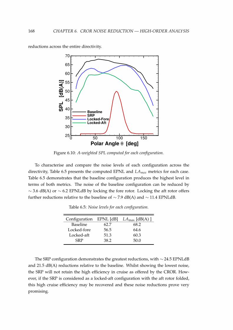
168 CHAPTER 6. CROR NOISE REDUCTION — HIGH-ORDER ANALYSIS
reductions across the entire directivity.
Polar Angle θ [deg]
SP
L
[dB
(A)]
0 50 100 15025
30
35
40
45
50
55
60
65
70
BaselineSRPLocked-ForeLocked-Aft
Figure 6.10: A-weighted SPL computed for each configuration.
To characterise and compare the noise levels of each configuration across thedirectivity, Table 6.5 presents the computed EPNL and LAmax metrics for each case.Table 6.5 demonstrates that the baseline configuration produces the highest level interms of both metrics. The noise of the baseline configuration can be reduced by∼ 3.6 dB(A) or ∼ 6.2 EPNLdB by locking the fore rotor. Locking the aft rotor offersfurther reductions relative to the baseline of ∼ 7.9 dB(A) and ∼ 11.4 EPNLdB.
Table 6.5: Noise levels for each configuration.
Configuration EPNL [dB] LAmax [dB(A) ]Baseline 62.7 68.2
Locked-fore 56.5 64.6Locked-aft 51.3 60.3
SRP 38.2 50.0
The SRP configuration demonstrates the greatest reductions, with ∼ 24.5 EPNLdBand 21.5 dB(A) reductions relative to the baseline. Whilst showing the lowest noise,the SRP will not retain the high efficiency in cruise as offered by the CROR. How-ever, if the SRP is considered as a locked-aft configuration with the aft rotor folded,this high cruise efficiency may be recovered and these noise reductions prove verypromising.

6.3. AEROACOUSTIC ANALYSIS 169
The components of each configuration are further studied to investigate the sourcesof the different noise level between each configuration. Therefore, to proceed, Fig-ure 6.11 presents the noise sources for the baseline configuration. From Figure 6.11a,it can firstly be observed that both fore and aft rotors retain high SPL values acrossthe polar directivity, highlighting the significance of the interaction component onboth rotors. The high contribution from both fore and aft rotors across the directivityfurther verifies the importance of both up and downstream interactions in the presentcase. Due to the equal rotational speed and blade count of fore and aft rotors, it isnot possible to extract the interaction component. However, the pressure derivativeterm of the Farassat loading source identifies the contribution due to unsteady load-ing. Furthermore, the equal loading of both rotors would suggest a similar level ofself-noise. Therefore, the observed differences will result from the interactions foreach blade row.
Figure 6.11b compares the loading and thickness contributions for the baselineconfiguration. The thickness contribution is shown to have a negligible contributionto the total noise across the entire directivity. This was found to be the case for allconfigurations, with the loading contribution dominating over the whole directivity.The thickness component would be expected to be more important as the relativevelocity of the rotors is increased.
Polar Angle θ [deg]
SP
L [
dB
(A)]
0 50 100 150
30
40
50
60
70
TotalForeAft
(a) Fore and aft rotor contributions
Polar Angle θ [deg]
SP
L [
dB
(A)]
0 50 100 150
30
40
50
60
70
TotalLoadingThickness
(b) Thickness and loading contributions
Figure 6.11: Noise components of the baseline configuration.
Figure 6.12 compares the contributions from fore and aft rotors for both locked-rotor configurations. For the locked-fore configuration, Figure 6.12a, with the excep-tion of the area near the rotor plane, the locked rotor makes a negligible contributionto the total noise. However, as the directivity approaches the rotor plane, the peak

170 CHAPTER 6. CROR NOISE REDUCTION — HIGH-ORDER ANALYSIS
levels of the locked rotor contribute significantly to the overall noise. The high noiselevels of the aft rotor across the directivity is indicative of the importance of the in-teraction from the locked fore rotor. In particular, the wake and potential interactionsfrom the stationary upstream blades.
Figure 6.12b compares the fore and aft contributions of the locked-aft configura-tion. It is interesting to note that in the locked-aft configurations, the locked rotor nowplays a more significant part in the total noise over a greater range of directivities.These similar levels result from sources. Firstly, relative to the locked-fore config-uration, the component of the locked rotor is increased. This increase arises fromthe downstream interactions from the operative fore rotor and is identified from thepressure derivative term in the Farassat formulation of the loading noise. Therefore,the interactions on the locked rotor are greater for the locked-aft configurations thanthe locked-fore configurations.
Secondly, relative to the locked-fore configuration, the operative rotor noise re-duces. The cause of this again relates to the interaction. In this case, the upstreaminteractions of the locked rotor are weaker. Therefore, it can be said that concerningthe locked rotor, the downstream interactions are more significant than the upstreaminteractions. These points highlight the importance of considering the design of thelocked rotor, something that was not observed when utilising the low-order models.
Polar Angle θ [deg]
SP
L [
dB
(A)]
0 50 100 150
30
40
50
60
70
TotalForeAft
(a) Locked-Fore
Polar Angle θ [deg]
SP
L [
dB
(A)]
0 50 100 150
30
40
50
60
70
TotalForeAft
(b) Locked-aft
Figure 6.12: Rotor noise contributions for locked-rotor configurations.
The significant levels of the locked rotors for both configurations can also bedescribed from the use of the A-weighting. Without weighting the operative rotor isthe dominant source over all observer angles. The locked rotor is less impacted by the

6.3. AEROACOUSTIC ANALYSIS 171
A-weighting due to higher levels at higher frequencies. The reductions in SPL of theoperative rotor due to the weighting therefore reduces its noise to levels comparableto the locked rotor, as observed in the figures above.
The azimuthal directivity is studied to investigate the noise of each configurationfurther. Figure 6.13 presents the computed azimuthal directivities of the baselineand SRP configurations. The A-weighting masked a number of the interesting fea-tures present for the current configurations. Therefore, to retain these features, theunweighted SPL is presented. Additionally, the scales have been adapted for eachconfiguration to highlight some of these features.
Figure 6.13a compares the contributions of fore and aft rotors for the baselineconfiguration. Both fore and aft rotors show an 8-peak response around the azimuth,owing to the simultaneous blade passage of this configuration. The peaks of the foreand aft directivities correspond to the peak loading, as shown in Figure 6.4a. Due tothe higher noise levels of the fore rotor, the total noise shows an 8-peak directivitypattern with peaks corresponding to those of the fore rotor.
Figure 6.13b demonstrates the continuous and symmetrical directivity pattern ofthe SRP configuration. This continuous pattern results from the steady assumptionsmade during the aerodynamic analysis.
ψ [deg]
SPL [dB]
0
30
60
90
120
150
180
210
240
270
300
330
90
TotalForeAft
(a) Baseline CROR
ψ [deg]
SPL [dB]
0
30
60
90
120
150
180
210
240
270
300
330
60 70 80 90
(b) SRP
Figure 6.13: Azimuthal directivity of baseline and SRP configuration.
Figure 6.14 compares the computed azimuthal directivity for the locked-rotorconfigurations. Figure 6.14a shows that over most angles, the noise of the locked-foreconfiguration is dominated by the operative aft rotor. The locked rotor shows aninteresting pattern around the azimuth formed of 4 distinctive peaks each composed

172 CHAPTER 6. CROR NOISE REDUCTION — HIGH-ORDER ANALYSIS
of two sub-peaks. These features arise from dominance of the contributions from thesecond and third harmonic components. Whilst the first harmonic component has a4 lobed pattern around the azimuth, the second and third harmonics show 8 lobesaround the azimuth. Additionally, the second and third harmonics show peak valuesgreater than that of the first harmonic. With the peaks of the first harmonic aligningwith every second trough of the second and third harmonics and the troughs of thefirst harmonic aligning with the troughs of every other trough of the second and thirdharmonics, the resulting trend shows the two sub-peaks followed by a large trough.
Figure 6.14b presents the azimuthal directivities of the locked-aft configuration.The fore rotor of the locked-aft configuration dominates the total noise over the entiredirectivity, not previously observed using the A-weighting. Whilst the locked rotorshows a negligible contribution to the overall noise, it presents an interesting 8-peakpattern around the azimuth, with peaks occurring every ∼ 45. This 8-peak patternarises due to the interaction with the potential field and wake from the fore rotor.
The analysis of the azimuthal directivity of all configurations has highlighted theinteractions between fore and aft rotors and their contributions to the total noise arenow also more clearly shown. In addition to this, the importance of the locked rotorcontribution is highlighted without the use of the A-weighting.
ψ [deg]
SPL [dB]
0
30
60
90
120
150
180
210
240
270
300
330
80 90
TotalForeAft
(a) Locked-fore
ψ [deg]
SPL [dB]
0
30
60
90
120
150
180
210
240
270
300
330
70 80 90
TotalForeAft
(b) Locked-aft
Figure 6.14: Azimuthal directivity of rotor components for locked-rotor configurations.
To study the interaction components further, the final element under investigationis the harmonic content of the sound. For this analysis, the frequency response ofall configurations is studied at the overhead position from the simulated flyover.Figure 6.15 compares the computed SPL up to the tenth harmonic of BPF for the

6.3. AEROACOUSTIC ANALYSIS 173
baseline and SRP configurations.Figure 6.15a shows high total SPL values across the harmonics for both fore and
aft rotors. The equal blade count and rotational rates of fore and aft rotors of thebaseline configuration mean that it is not possible to extract the interaction tones.However, the high values observed at higher harmonics indicate the importance ofthe interactions. Fore and aft rotors produce similar levels at the fundamental har-monic, resulting from similar self-noise. As the harmonics increase, the fore rotorhas the greatest contribution to the total noise for most harmonics. These increasedlevels at the higher harmonics further support the previous analysis showing the im-portance of the upstream interactions. Here, however, the increased values suggestthat in the present case, the upstream component is more significant than those trav-elling downstream. The high levels observed for increasing harmonics is contrary tothe almost continuous decay found for the isolated SRP configuration, Figure 6.15b.
Harmonic of BPF
SP
L [
dB
]
2 4 6 8 100
20
40
60
80TotalForeAft
(a) Baseline
Harmonic of BPF
SP
L [
dB
]
2 4 6 8 100
20
40
60
80
(b) SRP
Figure 6.15: Harmonic components of baseline and SRP configurations at the overheadposition.
Figure 6.16 compares the harmonic content of the locked-rotor configurations atthe overhead position. For the locked-fore configuration, Figure 6.16a shows that atthe overhead position the total SPL at each harmonic is generally not dominated byeither fore or aft (or operative or locked) rotor, but in fact, is comprised of significantcontributions from both rotors. The high values for both fore and aft rotors forincreasing harmonics is indicative of the importance of the interaction for both rotors.This fact also further highlights the importance of the contribution of the locked rotor.
Figure 6.16b compares the harmonic content of the locked-aft configurations at

174 CHAPTER 6. CROR NOISE REDUCTION — HIGH-ORDER ANALYSIS
the overhead position. For the locked-aft configuration, the fundamental and secondharmonic of BPF is dominated by the contribution from the operative rotor. However,as the harmonic increases, the locked rotor makes the most significant contributionfor the majority of harmonics. These high levels for the locked rotor result from theinteraction with the wake and potential field from the operative upstream rotor.
Comparing locked-fore and locked-aft configurations further, it is generally ob-served that the locked rotor of the locked-aft configuration has higher noise levelsdue to being in the wake of the upstream operative rotor. On the other hand, theoperative rotor of the locked-fore configuration generally shows higher levels due tobeing in the wake of the stationary upstream row. As a result, in the case of thelocked-rotor configurations, the downstream interactions are more important thanthose travelling upstream.
Harmonic of BPF
SP
L [
dB
]
2 4 6 8 100
20
40
60
80TotalForeAft
(a) Locked-fore
Harmonic of BPF
SP
L [
dB
]
2 4 6 8 100
20
40
60
80TotalForeAft
(b) Locked-aft
Figure 6.16: Harmonic components of locked-rotor configurations at the overhead position.
An acoustic analysis of the locked-rotor concept has been carried out. To quantifythe performance of the novel configurations, they have been compared with a base-line CROR (both rotors running). It was found that the lowest noise was achievedwith the locked-aft configuration. However, it could be reduced further when foldedback (as modelled by an isolated SRP). The analysis demonstrated the importance ofthe locked-rotor noise contribution, the significance of which was not generally ob-served in the low-order analysis and suggests a deficiency of the model. The lockedrotor was found to have a significant contribution across a number of harmonics anddirectivities. The analysis was carried out on a design of equal fore and aft blade

6.4. SUMMARY 175
count and therefore does not represent the most acoustically optimal configuration.As a result, future work should consider more acoustically optimal designs, e.g. un-equal blade count and rotor speeds.
6.4 Summary
The previous chapter identified the potential of the locked-rotor concept to re-duce CROR noise. In an attempt to further verify this potential, this chapter aimedat utilising high-order tools to investigate the novel concept. Firstly, an aerodynamicanalysis was carried out to ensure that each configuration could provide the requiredthrust. Each configuration could successfully deliver the required thrust with a smallpenalty in efficiency. Additionally, the locked-aft configuration was found to producea significant torque from the locked rotor. Further analysis is required to determinethe impact on performance to reduce this. A detailed study of the rotor loads high-lighted the equal importance of both up and downstream interactions.
An acoustic analysis further demonstrated the ability of the locked rotor conceptsto reduce CROR noise, with locked-fore and locked-aft configurations offering gainsof ∼ 3.6 and ∼ 7.9 dB(A) respectively. The lowest noise was, however, observed forthe SRP, with gains of ∼ 21.5 dB(A). The SRP does not meet the objectives of thesame cruise performance. However, if this is taken as the folded rotor concept, theresults are extremely positive. The analysis highlighted the importance of modellingthe locked rotor contribution, with further analysis required on reducing the contri-bution from the locked rotor. Additionally, the analysis should be extended to a moreacoustically optimal design to investigate further noise reductions for existing high-performing designs using the proposed concept. Furthermore, the present investi-gation, whilst confirming the low-order predictions, is only numerical. Therefore, tofully verify the noise-reducing potential of the proposed concepts, an experimentalstudy is required. Nonetheless, the present numerical analyses prove promising forthe reduction of CROR noise.

Chapter 7
Conclusions and Future Work
Increasing environmental pressures have resulted in a renewed interest in theCROR concept. However, amongst others, noise remains a pertinent issue for theCROR. A literature review identified that optimisation may be a useful resource toincorporate low-noise within the design. Additionally, the literature review foundthat the interaction noise component offered the greatest potential for noise reduc-tion. To this end, this thesis details the work carried out to develop and utilise nu-merical tools to investigate a number of novel configurations to reduce CROR noisefor general aviation aircraft.
The chapter proceeds by outlining the main conclusions of the presented work.Following this, a number of recommendations for future work are discussed.
7.1 Conclusions
There are a number of conclusions from the work presented within this thesis.These conclusions reflect the objectives outlined in the opening chapter of the thesis:
1. Develop a low-order, multi-disciplinary CROR design toolA number of low-order numerical tools for the analysis of CROR have been devel-
oped. Firstly, a BEMT model has been extended for the analysis of CROR. Secondly,an acoustic model to compute CROR noise has been implemented. The model iscoupled with the aerodynamic model and is capable of computing the important un-steady loading source. Validation and sensitivity studies for both aerodynamic andaeroacoustic models proved their ability to match reported data relatively well.
The models are coupled together in the form of a single design and analysis tool.The low execution time and the ability of the model to predict the required perfor-mance indicates this to be a useful preliminary design tool for CROR.
176

7.1. CONCLUSIONS 177
2. Demonstrate the use of the design tool to identify high-performing CROR de-signs for general aviation aircraft.
The low-order models have been implemented within a Genetic Algorithm op-timisation routine to incorporate low-noise into the design of a CROR for generalaviation.
The optimisation routine identified a number of designs with reduced noise rel-ative to a baseline configuration for three different design objectives. The optimisa-tion study found that low noise was achieved with large blade counts and reducedtip speeds. A multi-objective design considering take-off noise and cruise efficiencyidentified that these two objectives were competing. Nonetheless, a design with re-duced noise and increased efficiency was identified. Comparable results were alsofound when applying the design to civil aviation class aircraft.
Therefore, the coupling of the low-order models to an optimisation routine couldsuccessfully identify designs of low-noise. This result further highlights the ability ofthe preliminary design tools.
3. Use the low-order CROR design tool to investigate a number of novel configu-rations for reducing CROR noise in the terminal area.
The low-order design tools have been used to investigate the potential to reduceCROR noise using a novel multi-configuration CROR. In an effort to reduce the inter-action component, it is proposed to lock either fore or aft rotor in the terminal area.During cruise, the locked rotor is operated at design conditions to retain the highCROR efficiency. Investigating a large number of blade counts, locking either fore oraft rotor resulted in a maximum noise reduction of ∼ 3 dB(A) relative to the baselineconfiguration at take-off conditions. However, these came at the cost of ∼ 5% penaltyin efficiency. Furthermore, the lowest noise was obtained using a blade count of 6× 7for the baseline configuration.
Further noise reductions were sought by folding the locked-aft rotor backwardsand thus eliminating any interaction component. The folded-aft configuration of-fered further noise reductions of ∼ 10 dB(A). Additionally, offloading the operativerotor was considered by increasing the tip radius. The increased radius configura-tion demonstrated an ∼ 8 dB(A) reduction relative to a baseline with the same tipextension. Further gains would be envisioned from a reduction of the tip vortexcomponent.
Overall, the novel configurations proposed demonstrated significant noise reduc-tions relative to the baseline for a number of blade count combinations. These re-ductions prove promising for this preliminary analysis. However, these reductionsmust be further verified. Furthermore, the analysis considered these concepts from

178 CHAPTER 7. CONCLUSIONS AND FUTURE WORK
an acoustic point of view only and did not account for such things as the mechan-ical complexity, aerodynamic performance, etc. which must inevitably be weighedagainst the noise reductions.
4. Perform high-order aerodynamic analysis to investigate the noise sources ofthese novel concepts.
uRANS CFD simulations, using the HMB3 solver, were carried out on the base-line CROR configuration in addition to a number of locked-rotor configurations. Theanalysis confirmed the ability of the locked-rotor configurations to deliver the re-quired thrust. Furthermore, this was demonstrated to be delivered for a ∼ 5% ef-ficiency penalty. Additionally, the locked-aft configuration showed a large torquereaction for the locked rotor which must be further studied.
The aerodynamic analysis highlighted the importance of the interaction betweenblade rows. In particular, the equal importance of up- and downstream interactionsfor the operative rotors. The analysis suggested that the downstream interactions ofa locked rotor were stronger than those travelling upstream. As a result, fluctuatingloads on the operative rotor were higher on the locked-fore configuration. On theother hand, the fluctuating loads on the locked rotor were higher for the locked-aft configuration. The analysis also suggested that tip vortex interaction may be asignificant source for all configurations.
5. Use coupled high-order aerodynamic-aeroacoustic tools to verify the capabilitiesof the novel concepts.
Unsteady blade surface pressure from the CFD computations was used as input toan acoustic solver based on the Farassat 1A formulation to calculate the tonal noise ofeach configuration. The acoustic solver firstly confirmed the noise-reducing capabil-ities of the locked-rotor configuration. The locked-fore configuration demonstratednoise reductions of ∼ 3.5 dB(A), while the locked-aft showed reductions of ∼ 6.5dB(A) relative to the baseline configuration. Noise reductions were more significantfor the SRP, ∼ 17db(A). However, The SRP does not offer the required high cruiseperformance. Nonetheless, if this is representative of the folded-aft concept, it showspromising results. The acoustic analysis also highlighted an interesting observationthat the locked rotor can in fact make a significant contribution to the total noise.
Whilst noise reductions have been observed, the analysis presented here is purelynumerical, and an experimental study is required to verify the predictions. Fur-thermore, the present analysis was carried out for equal blade count and rotationalspeeds which perhaps does not represent the most acoustically optimal configura-tion. Therefore, to better quantify the potential of the proposed concept, additionalCROR configurations should be considered.

7.2. FUTURE WORK 179
To conclude, the aim of this thesis was to investigate a number of concepts toreduce CROR noise in the terminal area whilst retaining high efficiency. The conceptsproposed demonstrated the ability to reduce CROR noise through a reduction in theinteraction component. This resulted in an efficiency loss. However, this loss does notimpact the cruise segment and is, therefore, deemed acceptable. Hence, the presentedwork has, through the development and use of a number of numerical tools, met theobjectives set out at the beginning of the thesis.
7.2 Future Work
Whilst the present work has met the outlined objectives and investigated the abil-ity of a number of concepts to reduce CROR noise, there are a number of limitationsand areas of future work. In this section, recommendations for future work are de-scribed.
Firstly, while the low-order analysis identified a number of blade count combina-tions that offered noise reductions when either fore or aft row was locked. Ultimatelythough, the lowest noise was obtained for the baseline configuration. However, thiswas obtained from 6× 7 blades and may not be feasible for a general aviation classaircraft. Furthermore, the analysis was from an acoustic point of view only. There-fore, it would be interesting to use the optimisation routine to investigate furthernoise gains of the locked-rotor concepts from a multi-disciplinary approach.
The high-order analysis presented a number of interesting results. For example,the importance of the noise of the locked rotor was identified. Furthermore, theconfigurations considered were not acoustically optimal, e.g. equal blade counts, noclipping, etc. Therefore, further configurations should be studied to further realisethe potential of the proposed locked-rotor configurations. In particular, the effect ofthe blade count on the locked rotor should be further studied using the high-orderanalysis. This would give greater insight into the role of the locked rotor in the totalnoise generation and may support the development of the low-order models withhigh-order data.
Finally, the noise reductions found throughout the analysis have been from nu-merical analysis only. Therefore, these should be studied in experimentally to provethe noise reductions and the effect on CROR performance.

Appendix A
Appendix A - Broadband Noise
This supplementary section provides greater detail on the equations describingthe broadband noise sources. The equations presented here contain a large num-ber of terms. Therefore, to avoid adding an exhaustive list of further terms to thenomenclature, additional terms used in this section are described where used.
A.1 Trailing-Edge Source
The model described by Magliozzi [21] was used to compute the trailing-edgebroadband noise. Recall, from §3.3, the trailing-edge broadband noise is given by:
Spp(xxx,ω) =
(ωbz
2πc0σ2
)2
ly(ω)s|L|2Sqq(ω,0), (3.18)
where, ω is the radian frequency, ω = 2π f ; b and s are the semichord and semispan,respectively. ly is the spanwise correlation length, approximated as:
ly ≈2.1Uc
ω, (A.1)
with Uc the convection velocity. Returning to Equation (3.18), σ =√
x2 + β2z2 is thePradntl-Glauert transformed distance to the trailing-edge, with β = 1−M2. L is thegeneralised lift, given as:
|L|2 = (1 + Mc −M)Dσ4
z2Mcrl2Kx
2 , (A.2)
where the directivity factor, D is:
D =2cos2(θ/2)
[1− (M−Mc)cos(θ)]2(1−M cosθ)(A.3)
180
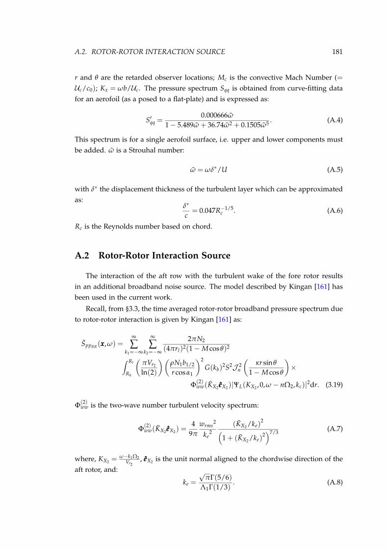
A.2. ROTOR-ROTOR INTERACTION SOURCE 181
r and θ are the retarded observer locations; Mc is the convective Mach Number (=Uc/c0); Kx = ωb/Uc. The pressure spectrum Sqq is obtained from curve-fitting datafor an aerofoil (as a posed to a flat-plate) and is expressed as:
S′qq =0.000666ω
1− 5.489ω + 36.74ω2 + 0.1505ω5 . (A.4)
This spectrum is for a single aerofoil surface, i.e. upper and lower components mustbe added. ω is a Strouhal number:
ω = ωδ∗/U (A.5)
with δ∗ the displacement thickness of the turbulent layer which can be approximatedas:
δ∗
c= 0.047R−1/5
c . (A.6)
Rc is the Reynolds number based on chord.
A.2 Rotor-Rotor Interaction Source
The interaction of the aft row with the turbulent wake of the fore rotor resultsin an additional broadband noise source. The model described by Kingan [161] hasbeen used in the current work.
Recall, from §3.3, the time averaged rotor-rotor broadband pressure spectrum dueto rotor-rotor interaction is given by Kingan [161] as:
SppRR(xxx,ω) =∞
∑k1=−∞
∞
∑k2=−∞
2πN2
(4πrl)2(1−M cosθ)2
∫ Rt
Rh
(πVr2
ln(2)
)(ρN1b1/2
r cosα1
)2
G(kb)2S2J 2
n
(κr sinθ
1−M cosθ
)×
Φ(2)ww(KX2 eeeX2)|ΨL(KX2 ,0,ω− nΩ2,kc)|2dr. (3.19)
Φ(2)ww is the two-wave number turbulent velocity spectrum:
Φ(2)ww(KX2 eeeX2) =
49π
wrms2
ke2
(KX2 /ke)2(
1 + (KX2 /ke)2)7/3 (A.7)
where, KX2 =ω−k1Ω2
Vr2, eeeX2 is the unit normal aligned to the chordwise direction of the
aft rotor, and:
ke =
√πΓ(5/6)
Λ1Γ(1/3). (A.8)

182 APPENDIX A. APPENDIX A - BROADBAND NOISE
Λ1 is the integral lengthscale, Λ1 ∼ 0.42b 12
and Γ(·) is the Gamma function (See p.255of Ref. [97]). b 1
2is the wake half width:
b 12= 0.25
√cd1 c1Lw (A.9)
with cd1 , c1 and Lw the fore drag coefficient, fore chord, and Lw = (g− c22 cos β2)/cos β1
is the wake helical length, where g, β1 and β2 are the axial rotor spacing and fore andaft setting angles respectively.
As estimated from Blandeau [162], wrms ∼ 0.404ude f ; where, ude f is the wake cen-treline velocity deficit:
ude f = 2Vr1
√cd1 c1 ln(2)
πLw(A.10)
Returning to Equation (3.19),
G(kb) = exp
− kb
2
4ln(2)
, (A.11)
is the normalised Fourier coefficient for the wavenumber kb,
kb =k2N1b 1
2
r cos β1. (A.12)
S is defined as:S =
c2
2
[κ cosθl sin β2
1−M cosθl− k1 cos β2
r
](A.13)
where κ = ω/c0, and J is the Bessel function.
Finally, ΨL is the acoustically weighted lift function. The lift function is computedaccording to the frequency of the gust, for low frequency gusts, i.e.: |σ|Mr2
βr22 < π
4 ,
ΨL(KX2 ,0,ω,kc) =1
βr2
S(
σ
β2r2
)exp
j
σ
βr2
f (Mr2)
[J0(η
′)− jJ1(η′)]
. (A.14)
For high frequency gusts, i.e.: |σ|Mr2βr2
2 > π4
ΨL(KX2 ,0,ω,kc) =
√2µ′
expjkc + jσπ (1 + Mr2)
12 (jσ)
12
E∗[√
4µ′
π
]. (A.15)
where:βr2 =
√1 = Mr2
2,
f (Mr2) = (1− βr2) ln(Mr2) + βr2 ln(1 + βr2)− ln(2)

A.2. ROTOR-ROTOR INTERACTION SOURCE 183
σ = 0.5KX2 c2
S is the Sears’ function:S =
1jx[K0(jx) + K1 jx]
. (A.16)
η′ and µ′ are given by:
η′ =σMr2
2
βr2
− kc,
µ′ =σMr2
1 + Mr2
+ kc
(A.17)
kc is:
kc =c2
2
[κ cosθl cosφ2
1−M cosθl+
nr2
sinφ2
]. (A.18)

Bibliography
[1] L. H. Smith, “Unducted Fan Aerodynamic Design,” Journal of Turbomachinery,vol. 109, 1987. doi: 10.1115/1.3262108
[2] A. B. Parry and S. Vianello, “A project study of open rotor noise,” InternationalJournal of Aeroacoustics, vol. 11, no. 2, pp. 247–258, 2012. doi: 10.1260/1475-472X.11.2.247
[3] S. Guerin, R. Schnell, and R. G. Becker, “Performance prediction and progresstowards multi-disciplinary design of contra-rotating open rotors,” AeronauticalJournal, vol. 118, no. 1208, pp. 1159–1179, 2014. doi: 10.1017/S0001924000009830
[4] D. E. Van Zante, F. Collier, A. Orton, S. A. Khalid, J. P. Wojno, and T. H.Wood, “Progress in open rotor propulsors: The FAA/GE/NASA open rotortest campaign,” Aeronautical Journal, vol. 118, no. 1208, pp. 1181–1213, 2014.doi: 10.1017/S0001924000009842
[5] F. W. Lanchester, “Investigation of the Efficiency of Reverse Rotating Propellersin Tandem,” British ARC RM No. 540, 1918.
[6] F. Lanchester, “Contra-Props,” Flight Magazine, pp. 418–419, 1941.
[7] R. D. Hager and D. Vrabel, “Advanced Turboprop Project,” NASA SP-495, 1988.
[8] B. S. Gatzen and C. N. Reynolds, “Single Rotation and Counter Rotation Prop-Fan Propulsion System Technologies.” in Congress of the International Council ofthe Aeronautical Sciences, vol. 2, 1984. ISBN 0915928892 (ISBN) pp. 708–717.
[9] J. Godston and C. N. Reynolds, “Future prop-fans - Tractor or pusher,” in AIAA21st Joint Propulsion Conference, 1985. doi: 10.2514/6.1985-1189
[10] A. F. El-Sayed, Fundamentals of Aircraft and Rocket Propulsion. London: Springer-Verlag, 2016. ISBN 9781447167969
[11] V. M. Moores, “Pratt Whitney considers geared open rotorconcept,” 2007. [Online]. Available: https://www.flightglobal.com/pratt-and-whitney-considers-geared-open-rotor-concept/74840.article
184
BIBLIOGRAPHY 185
[12] Commission of the European Communities, “An Agenda for Sustainable Fu-ture in General and Business Aviation - Communication from the Commis-sion,” 2007.
[13] Council of the European Union, “Council Conclusions on the Commissioncommunication on an agenda for sustainable future in general and businessaviation,” in 2861st Transport, Telecommunications and Energy Council Meeting,Luxembourg, 2008.
[14] M. Newton, “Private Communication,” 2017.
[15] D. E. Van Zante, “Progress in Open Rotor Research: A U.S. Perspective,” inASME Turbo Expo 2015, Montreal, Canada, 2015. doi: 10.1115/GT2015-42203.ISBN 9780791856628 pp. 1–14.
[16] N. Peake and A. B. Parry, “Modern Challenges Facing Turbomachinery Aeroa-coustics,” Annual Review of Fluid Mechanics, vol. 44, no. 1, pp. 227–248, 2012.doi: 10.1146/annurev-fluid-120710-101231
[17] European Comission, “Sustainable and Green Engines (SAGE)— Clean Sky.” [Online]. Available: http://www.cleansky.eu/sustainable-and-green-engines-sage
[18] D. B. Hanson, “Influence of Propeller Design Parameters on Far-Field Har-monic Noise in Forward Flight,” AIAA Journal, vol. 18, no. 11, pp. 1313–1319,1980. doi: 10.2514/3.50887
[19] J. H. Dittmar, “Some Design Philosophy for Reducing the Community Noise ofAdvanced Counter- Rotation Propellers,” NASA TM 87099, 1985.
[20] C. Hall, A. Zachariadis, T. Brandvik, and N. Sohoni, “How to Improve OpenRotor Aerodynamics at Cruise and Take-Off,” Aeronautical Journal, vol. 118, no.1208, pp. 1103–1123, 2014. doi: 10.1017/S0001924000009805
[21] B. Magliozzi, D. B. Hanson, and R. K. Amiet, “Propeller and Propfan Noise,”NASA Langley Research Center, Aeroacoustics of Flight Vehicles: Theory and Practice.Volume 1: Noise Sources, 1991.
[22] J. H. Dittmar, R. J. Jeracki, and B. J. Blaha, Tone Noise of Three Supersonic HelicalTip Speed Propellers in a Wind Tunnel, 1980. ISBN 1979001766
[23] J. H. Dittmar, “A Comparison Between an Existing Propeller Noise Theory andWind Tunnel Data,” NASA TM 81519, 1980.

186 BIBLIOGRAPHY
[24] F. Farassat and G. P. Succi, “Theory of Noise Generation From Moving BodiesWith and Application to Helicopter Rotors,” NASA TR R-451, 1975.
[25] F. Farassat, “Discontinuities in aerodynamics and aeroacoustics: The conceptand applications of generalized derivatives,” Journal of Sound and Vibration,vol. 55, no. 2, pp. 165–193, 1977. doi: 10.1016/0022-460X(77)90593-4
[26] F. Farassat, C. E. K. Morris Jr, and P. A. Nystrom, “A comparison of linearacoustic theory with experimental noise data for a small-scale hovering rotor,”in American Institute of Aeronautics and Astronautics 5th Aeroacoustics Conference,1979.
[27] J. C. Simonich, D. C. McCormick, and P. L. Lavrich, “Role of leading-edgevortex flows in prop-fan interaction noise,” Journal of Aircraft, vol. 30, no. 2, pp.255–261, 1993. doi: 10.2514/3.48274
[28] A. Zachariadis, C. Hall, and A. B. Parry, “Contrarotating Open Rotor Operationfor Improved Aerodynamics and Noise at Takeoff,” Journal of Turbomachinery,vol. 135, 2013. doi: 10.1115/1.4006778
[29] D. B. Hanson, “Noise of Counter-Rotation Propellers with Non-SynchronousRotors,” Journal of Aircraft, vol. 22, no. 12, pp. 1097–1099, 1985.doi: 10.2514/3.45173
[30] C. K. W. Tam, M. Salikuddin, and D. B. Hanson, “Acoustic Interference ofCounter-Rotating Propellers,” Journal of Sound and Vibration, vol. 124, no. 2, pp.357–366, 1988.
[31] G. Delattre and F. Falissard, “Influence of Torque Ratio on Counter-RotatingOpen-Rotor Interaction Noise,” AIAA Journal, vol. 53, no. 9, pp. 2726–2738,2015. doi: 10.2514/1.J053797
[32] A. Peters and Z. S. Spakovszky, “Rotor Interaction Noise in Counter-RotatingPropfan Propulsion Systems,” Journal of Turbomachinery, vol. 134, no. 1, pp.2821–2834, 2010. doi: 10.1115/GT2010-22554
[33] R. P. Woodward, “Noise of a Model High Speed Counterrotation Propeller atSimulated Takeoff/Approach Conditions (F7/A7),” NASA TM 100206, 1987.
[34] R. P. Woodward and E. B. Gordon, “Noise of a Model Counterrotation PropellerWith Reduced Aft Rotor Diameter and Simulated Takeoff/Approach Condi-tions (F7/A3).” in 26th Aerospace Sciences Meeting, 1988. doi: 10.2514/6.1988-263.ISSN 04999320

BIBLIOGRAPHY 187
[35] J. H. Dittmar and D. B. Stang, “Reduction of the noise of a model counterrota-tion propeller at cruise by reducing the aft propeller diameter,” The Journal ofthe Acoustical Society of America, vol. 81, no. S1, 1987. doi: 10.1121/1.2024493
[36] R. K. Majjigi, K. Uenishi, and P. R. Gliebe, “An Investigation of CounterrotatingTip Vortex Interaction,” NASA CR 185135, 1989.
[37] M. J. Kingan and R. H. Self, “Counter-Rotation Propeller Tip Vortex InteractionNoise,” in 15th AIAA/CEAS Aeroacoustics Conference (30th AIAA AeroacousticsConference), 2009. doi: 10.2514/6.2009-3135. ISBN 978-1-60086-967-9
[38] M. E. Quaglia, T. Leonard, S. Moreau, and M. Roger, “A 3D analytical modelfor orthogonal blade-vortex interaction noise,” Journal of Sound and Vibration,vol. 399, pp. 104–123, 2017. doi: 10.1016/j.jsv.2017.03.023
[39] J. H. Dittmar, “The Effect of Front-to-Rear Propeller Spacing on the InteractionNoise of a Model Counterrotation Propeller at Cruise Conditions,” NASA TM100121, 1987.
[40] A. B. Parry, “Theoretical Prediction of Counter-Rotating Propeller Noise,” PhDThesis, University of Leeds, 1988.
[41] A. B. Parry and D. G. Crighton, “Asymptotic theory of propeller noise. I -Subsonic single-rotation propeller,” AIAA Journal, vol. 27, no. 9, pp. 1184–1190,1989. doi: 10.2514/3.10244
[42] S. A. Khalid, J. P. Wojno, A. Breeze-Stringfellow, D. P. Lurie, T. H. Wood,K. Ramakrishnan, and U. Paliath, “Open rotor designs for low noise andhigh efficiency,” Proceedings of the ASME Turbo Expo, vol. 6 C, pp. 1–14, 2013.doi: 10.1115/GT2013-94736
[43] G. Delattre and F. Falissard, “Aerodynamic and acoustic impacts of a singleprotuberance placed on the leading edge of the front blades of an open rotor,”48th International Symposium of Applied Aerodynamics of Small Bodies and Details,2013.
[44] G. Delattre, F. Falissard, L. Vion, and L. Jacquin, “Open rotor interaction noisereduction through front rotor wake modification,” International Journal of Aeroa-coustics, vol. 15, no. 1-2, pp. 207–227, 2016. doi: 10.1177/1475472X16643461
[45] P. Gardarein, “Calculs aerodynamiques des helices rapides transsoniques,” in28 eme Colloque d’Aerodynamique Appliquee, Saint-Louis, France, 1991.

188 BIBLIOGRAPHY
[46] L. Cambier, “Status of the elsA CFD Software for Flow Simulation and Multi-disciplinary Applications,” in 46th AIAA Aerospace Sciences Meeting and Exhibit,Reno, Nevada, 2008.
[47] L. Cambier, S. Heib, and S. Plot, “The Onera elsA CFD software: input fromresearch and feedback from industry,” Mechanics & Industry, vol. 14, no. 3, pp.159–174, 2013. doi: 10.1051/meca/2013056
[48] R. Boisard, G. Delattre, and F. Falissard, “Computational Fluid Dynamics as aSupport to Counter-Rotating Open-Rotor Wind-Tunnel Test Analysis,” Journalof Aircraft, vol. 51, no. 2, pp. 614–628, 2014. doi: 10.2514/1.C032348
[49] L. Vion, G. Delattre, F. Falissard, and L. Jacquin, “Counter-Rotating OpenRotor (CROR): Flow Physics and Simulation,” in 20eme Congres Francais deMecaniqueais de Mecanique, Besancon, 2011.
[50] R. Jaron, A. Moreau, S. Guerin, and R. Schnell, “Optimization of trailing-edge serrations to reduce open-rotor tonal interaction noise,” Journal of Flu-ids Engineering, Transactions of the ASME, vol. 140, no. 2, pp. 1–8, 2018.doi: 10.1115/1.4037981
[51] C. Weckmuller and S. Guerin, “On the influence of trailing-edge serrationson open-rotor tonal noise,” in 18th AIAA/CEAS Aeroacoustics Conference, 2012.doi: 10.2514/6.2012-2124
[52] C. A. Negulescu, “Airbus AI-PX7 CROR Design Features and Aerodynam-ics,” SAE International Journal of Aerospace, vol. 6, no. 2, pp. 626–642, 2013.doi: 10.4271/2013-01-2245
[53] G. N. Barakos and C. S. Johnson, “Acoustic comparison of propellers,”International Journal of Aeroacoustics, vol. 15, no. 6-7, pp. 575–594, 2016.doi: 10.1177/1475472X16659214
[54] G. Chirico, G. N. Barakos, and N. Bown, “Numerical aeroacoustic analysis ofpropeller designs,” Aeronautical Journal, vol. 122, no. 1248, pp. 283–315, 2018.doi: 10.1017/aer.2017.123
[55] I. Lepot, M. Leborgne, R. Schnell, J. Yin, G. Delattre, F. Falissard, and J. Tal-botec, “Aero-Mechanical Optimization of a Contra-Rotating Open Rotor andAssessment of its Aerodynamic and Acoustic Characteristics,” Proceedings ofthe Institution of Mechanical Engineers Part a-Journal of Power and Energy, vol. 225,no. A7, pp. 850–863, 2011. doi: 10.1177/0957650911413695

BIBLIOGRAPHY 189
[56] R. Schnell, J. Yin, C. Voss, and E. Nicke, “Assessment and Optimization of theAerodynamic and Acoustic Characteristics of a Counter Rotating Open Rotor,”Journal of Turbomachinery, vol. 134, no. 6, 2012. doi: 10.1115/1.4006285
[57] G. Montero Villar, D. Lindblad, and N. Andersson, “Multi-Objective Optimiza-tion of a Counter Rotating Open Rotor using Evolutionary Algorithms,” 2018Multidisciplinary Analysis and Optimization Conference, 2018. doi: 10.2514/6.2018-2929
[58] G. Grasso, S. Moreau, J. Christophe, and C. Schram, “Multi-disciplinary opti-mization of a contra-rotating fan,” International Journal of Aeroacoustics, vol. 17,no. 6-8, pp. 655–686, 2018. doi: 10.1177/1475472X18789000
[59] R. A. D. Akkermans, A. Stuermer, and J. W. Delfs, “Assessment of Front-RotorTrailing-Edge-Blowing for the Reduction of Open Rotor Noise Emissions,” in19th AIAA/CEAS Aeroacoustics Conference, 2013. doi: 10.2514/6.2013-2200
[60] A. Sturmer and R. A. D. Akkermans, “Multidisciplinary analysis of CRORpropulsion systems: DLR activities in the JTI SFWA project,” CEAS AeronauticalJournal, vol. 5, no. 3, pp. 265–277, 2014. doi: 10.1007/s13272-014-0105-4
[61] A. Stuermer, R. A. D. Akkermans, and J. W. Delfs, “Assessment of front rotortrailing edge blowing for the reduction of open rotor interaction noise,” inNotes on Numerical Fluid Mechanics and Multidisciplinary Design, 2014, vol. 124,pp. 609–618.
[62] R. A. Akkermans, A. W. Stuermer, and J. Delfs, “Active Flow Control for In-teraction Noise Reduction of Contra-Rotating Open Rotors,” in 49th AIAA/AS-ME/SAE/ASEE Joint Propulsion Conference. Reston, Virginia: American Instituteof Aeronautics and Astronautics, jul 2013. doi: 10.2514/6.2013-3799. ISBN 978-1-62410-222-6
[63] R. A. D. Akkermans, A. Stuermer, and J. W. Delfs, “Active Flow Control forInteraction Noise Reduction of Contra-Rotating Open Rotors,” AIAA Journal,vol. 54, no. 4, pp. 1413–1423, 2016. doi: 10.2514/1.J053756
[64] A. Stuermer and J. Yin, “Aerodynamic and Aeroacoustic Installation Effectsfor Pusher-Configuration CROR Propulsion Systems,” in 28th AIAA AppliedAerodynamics Conference, 2010. doi: 10.2514/6.2010-4235
[65] T. Gerhold, “Overview of the Hybrid RANS Code TAU,” Kroll N., FassbenderJ.K. (eds) MEGAFLOW - Numerical Flow Simulation for Aircraft Design. Notes on

190 BIBLIOGRAPHY
Numerical Fluid Mechanics and Multidisciplinary Design (NNFM), vol. 89, pp. 81–92, 2006. doi: 10.1007/3-540-32382-1˙5
[66] J. Yin and J. Delfs, “Improvement of DLR Rotor Aeroacoustic Code (APSIM)and its Validation with Analytic Solution,” in 29th European Rotorcraft Forum,Friedrichshafen, Germany, 2003.
[67] A. Stuermer, “Validation of uRANS-simulations of contra-rotating open rotor-powered aircraft at take-off conditions,” AIAA Aerospace Sciences Meeting, 2018,no. 210059, 2018. doi: 10.2514/6.2018-1265
[68] J. Kleinert, L. Durrwachter, M. Keßler, and E. Kramer, “Aeroacoustics of High-Fidelity URANS Simulations of a Model Contra-Rotating Open Rotor withMounting Pylon,” 2018 AIAA/CEAS Aeroacoustics Conference, pp. 1–17, 2018.doi: 10.2514/6.2018-4082
[69] G. L. Gentry Jr., E. R. Booth Jr., and M. A. Takallu, “Effect of Pylon Wake Withand Without Pylon Blowing on Propeller Thrust,” NASA TM 4162, 1990.
[70] B. Shivashankara, D. Johnson, and R. Cuthberston, “Installation Effect onCounter Rotation Propeller Noise S,” in AIAA 13th Aeroacoustics Conference,1990. doi: 10.2514/6.1990-4023
[71] J. Ricouard, E. Julliard, M. Omais, V. Regnier, A. B. Parry, and S. Baralon,“Installation Effects on Contra-Rotating Open Rotor Noise,” 16th AIAA/CEASAeroacoustics Conference, no. August 2015, pp. 1–8, 2010. doi: 10.2514/6.2010-3795
[72] A. Stuermer, J. Yin, and R. Akkermans, “Progress in aerodynamic and aeroa-coustic integration of CROR propulsion systems,” Aeronautical Journal, vol. 118,no. 1208, pp. 1137–1158, 2014. doi: 10.1017/S0001924000009829
[73] M. J. Kingan, C. Powles, and R. H. Self, “Effect of Centerbody Scatter-ing on Advanced Open-Rotor Noise,” AIAA JOURNAL, vol. 48, no. 5, 2010.doi: 10.2514/1.44659
[74] M. J. Kingan and P. Sureshkumar, “Open rotor centrebody scatter-ing,” Journal of Sound and Vibration, vol. 333, no. 2, pp. 418–433, 2014.doi: 10.1016/j.jsv.2013.08.010
[75] M. Lummer, C. Richter, C. Proeber, and J. Delfs, “Validation of a Model forOpen Rotor Noise Predictions and Calculation of Shielding Effects using a FastBEM,” 19th AIAA/CEAS Aeroacoustics Conference, 2013. doi: 10.2514/6.2013-2096

BIBLIOGRAPHY 191
[76] L. Sanders, D. C. Mincu, W. Denis, P. L. Vitagliano, M. Minervino, J. Kennedy,P. Eret, and G. Bennett, “A coupling of computational methods for CRORinstallation effects,” in 20th AIAA/CEAS Aeroacoustics Conference AIAA, 2014.doi: 10.2514/6.2014-3190. ISBN 9781624102851
[77] L. Sanders, D. C. Mincu, P. L. Vitagliano, M. Minervino, J. Kennedy, and G. Ben-nett, “Prediction of the acoustic shielding by aircraft empennage for contra-rotating open rotors,” International Journal of Aeroacoustics, vol. 16, no. 7-8, pp.626–648, 2017. doi: 10.1177/1475472X17734334
[78] Y. Guo and R. H. Thomas, “Experimental study on open rotor noise shieldingby hybrid-wing-body aircraft,” AIAA Journal, vol. 54, no. 1, pp. 242–253, 2016.doi: 10.2514/1.J054243
[79] European Commission, “Final Report Summary - WENEMOR,” 2020. [Online].Available: https://cordis.europa.eu/project/id/278419/reporting
[80] J. Kennedy, P. Eret, and G. J. Bennett, “A parametric study of airframeeffects on the noise emission from installed contra-rotating open rotors,”International Journal of Aeroacoustics, vol. 17(6–8) 62, pp. 624–654, 2018.doi: 10.1177/1475472X18789003
[81] L. Durrwachter, M. Keßler, and E. Kramer, “Numerical Assessment of Open-Rotor Noise Shielding with a Coupled Approach,” AIAA Journal, vol. 57, no. 5,pp. 1930–1940, 2019. doi: 10.2514/1.j057531
[82] R. Froude, “On the part played in propulsion by differences of fluid pressure,”13th Session of the Institution of Naval Architects, vol. 30, pp. 390–405, 1889.
[83] W. J. M. Rankine, “On the Mechanical Priciples of the Action of Propellers,”Transactions of the Institution of Naval Architects, vol. 6, pp. 1–18, 1865.
[84] H. Glauert, The elements of airfoil and airscrew theory, 2nd ed. Cambridge Uni-versity Press, 1926. ISBN 9788578110796
[85] P. M. Sforza, “Propellers,” Theory of Aerospace Propulsion, pp. 409–437, 2012.doi: 10.1016/B978-1-85617-912-6.00010-4
[86] R. D. Harrington, “Full-Scale-Tunnel Investigation of the Static-Thrust Perfor-mance of a Coaxial Helicopter Rotor,” NACA TN 2318, 1951.
[87] A. Betz, “Schraubenpropeller mit geringstem Energieverlust. Mit einem Zusatzvon L. Prandtl,” Nachrichten von der Gesellschaft der Wissenschaften zu Gottingen,Mathematisch-Physikalische Klasse, vol. Bd. 3, pp. 193–217, 1919.
192 BIBLIOGRAPHY
[88] L. Prandtl, “Appliction of Hydrodynamics to Modern Aeronautics,” NACAReport No. 116, Tech. Rep., 1921.
[89] H. Glauert, “Airplane Propellers,” in Aerodynamic Theory. Berlin, Heidelberg:Springer Berlin Heidelberg, 1935, pp. 169–360. ISBN 9783642896309
[90] P. Beaumier, “A Low Order Method for Co-Axial Propeller and Rotor Perfor-mance Prediction,” 29th Congrees of the International Council of the Aerautical Sci-ences (ICAS 2014), 2014.
[91] B. W. McCormick, Aerodynamics of V/STOL Flight. London Academic Press,1967.
[92] R. L. Burden and J. D. Faires, “Numerical Solutions of Nonlinear Systems ofEquaitons,” in Numerical Analysis, 9th ed. Cengage Learning, Brooks/Cole,2010, pp. 629–669.
[93] S. C. Chapra, “Numerical Differentiation,” in Applied Numerical Methods withMATLAB for Engineers and Scientists, 3rd ed. McGraw-Hill Education, 2012,pp. 521–546.
[94] K. Levenberg, “A Method for the Solution of Certain Non-Linear Problems inLeast Squares,” Quarterly of Applied Mathematics, vol. 2, no. 2, pp. 164–168, 1944.
[95] D. W. Marquardt, “AN ALGORITHM FOR LEAST-SQUARES ESTIMA-TION OF NONLINEAR PARAMETERS,” Journal of the society for In-dustrial and Applied Mathematics, vol. 11, no. 2, pp. 431–441, 1963.doi: 10.1017/CBO9781107415324.004
[96] J. J. More, “The Levenberg-Marquardt Algorithm: Implementation and The-ory,” in Lecture Notes in Mathematics 630. Springer Verlag, 1977, pp. 105–116.
[97] M. Abramowitz and I. A. Stegun, Handbook of Mathematical Functions, 10th ed.Washington D.C: National Bureau of Standards, 1964.
[98] A. B. Parry, “Modular Prediction Scheme for Blade Row InteractionNoise,” Journal of Propulsion and Power, vol. 13, no. 3, pp. 334–341, 1997.doi: 10.2514/2.5186
[99] C. M. Ekoule, A. McAlpine, A. B. Parry, M. J. Kingan, and N. Sohoni, “De-velopment of a Hybrid Method for the Prediction of Advanced Open RotorTone Noise,” 23rd AIAA/CEAS Aeroacoustics Conference, no. June, pp. 1–15, 2017.doi: 10.2514/6.2017-3870

BIBLIOGRAPHY 193
[100] I. H. Abott and A. E. von Doenhoff, Theory of Wing Sections Including a Summaryof Airfoil Data. Dover Publications, 1959.
[101] F. J. Bailey, “A Simplified Theoretical Method of Determining the Characteris-tics of a Lifting Rotor in Forward Flight,” NACA Report No. 716, 1941.
[102] A. Filippone, “Rapid Estimation of Airfoil Aerodynamics for Helicopter Ro-tors,” Journal of Aircraft, vol. 45, no. 4, pp. 1468–1472, 2008. doi: 10.2514/1.35560
[103] T. A. Egolf, O. L. Anderson, D. E. Edwards, and A. J. Landgrebe, “Analysisfor high speed propeller-nacelle aerodynamic performance prediction: VolumeII-user’s manual,” NASA Contractor Report 4199, no. 4199, 1988.
[104] W. Z. Stepniewski and C. N. Keys, “Vortex Theory,” in Rotary-Wing Aerodynam-ics, 2nd ed., 1979, ch. 4, pp. 141–232.
[105] J. G. Leishman, “Aerodynamics of Rotor Aerofoils,” in Principles of HelicopterAerodynamics, 2nd ed., 2006, pp. 347–422.
[106] D. M. Dunham, C. L. Gentry, and P. L. Coe, “Low-Speed Wind-Tunnel Tests ofSingle- and Counter-Rotation Propellers,” NASA TM-87656, 1986.
[107] R. J. Jeracki, D. C. Mikkelson, and B. J. Blaha, “Wind Tunnel Performance ofFour Energy Efficient Propellers Designed for Mach 0.8 Cruise,” NASA TM-79124, 1979. doi: 10.4271/790573
[108] A. Zachariadis and C. Hall, “Application of a Navier–Stokes Solver to theStudy of Open Rotor Aerodynamics,” Journal of Turbomachinery, vol. 133, 2011.doi: 10.1115/1.4001246
[109] G. Barakos, R. Steijl, K. Badcock, and A. Brocklehurst, “Development of CFDCapability for Full Helicopter Engineering Analysis,” 31st European RotorcraftForum, 2005.
[110] R. Steijl, G. Barakos, and K. Badcock, “A Framework for CFD Analysis of Heli-copter Rotors in Hover and Forward Flight.” International Journal for NumericalMethods in Fluids, vol. 51, no. 8, pp. 819–847, 2006. doi: 10.1002/fld.1086
[111] C. Hirt, A. Amsden, and J. Cook, “An Arbitrary Lagrangian-Eulerian Com-puting Method for All Flow Speeds,” Journal of Computational Physics, vol. 135,no. 2, pp. 203–216, 1997. doi: 10.1006/jcph.1997.5702

194 BIBLIOGRAPHY
[112] S. Osher and S. Chakravarthy, “Upwind schemes and boundary conditionswith applications to Euler equations in general geometries,” Journal of Computa-tional Physics, vol. 50, no. 3, pp. 447–481, 1983. doi: 10.1016/0021-9991(83)90106-7
[113] B. van Leer, “Towards the ultimate conservative difference scheme. V. A second-order sequel to Godunov’s method,” Journal of Computational Physics, vol. 32,no. 1, pp. 101–136, 1979. doi: 10.1016/0021-9991(79)90145-1
[114] G. D. van Albada, B. van Leer, and W. W. Roberts Jr., “A Comparative Study ofComputational Methods in Cosmic Gas Dynamics,” Astronomy and Astrophysics,vol. 108, no. 1, pp. 76–84, 1982. doi: 10.1007/978-3-642-60543-7˙6
[115] A. Jameson, “Time dependent calculations using multigrid, with applicationsto unsteady flows past airfoils and wings,” 10th Computational Fluid DynamicsConference, 1991, 1991. doi: 10.2514/6.1991-1596
[116] O. Axelsson, Iterative Solution Methods. Cambridge University Press, 1994.
[117] D. C. Wilcox, “Reassessment of the Scale-Determining Equation for AdvancedTurbulence Models,” AIAA Journal, vol. 26, no. 11, pp. 1299–1310, 1988.doi: 10.2514/3.10041
[118] F. R. Menter, “Two-equation eddy-viscosity turbulence models for engi-neering applications,” AIAA Journal, vol. 32, no. 8, pp. 1598–1605, 1994.doi: 10.2514/3.12149
[119] B. Launder and D. Spalding, “The Numerical Computation of TurbulentFlows,” Computer Methods in Applied Mechanics and Engineering, vol. 3, no. 2,pp. 269–289, 1974. doi: 10.1016/0045-7825(74)90029-2
[120] F. R. Menter, M. Kuntz, and R. Bender, “A Scale-Adaptive Simulation Model forTurbulent Flow Predictions,” in 41st Aerospace Science Meeting & Exhibit, 2003.doi: 10.2514/6.2003-767
[121] F. R. Menter and Y. Egorov, “The scale-adaptive simulation method for un-steady turbulent flow predictions. part 1: Theory and model description,” Flow,Turbulence and Combustion, vol. 85, no. 1, pp. 113–138, 2010. doi: 10.1007/s10494-010-9264-5
[122] G. Chirico, “Aeroacoustic Simulation of Modern Propellers,” PhD Thesis, Uni-versity of Glasgow, 2018.

BIBLIOGRAPHY 195
[123] R. Steijl and G. Barakos, “Sliding Mesh Algorithm for CFD Analysis of Heli-copter Rotor–Fuselage Aerodynamics,” International Journal for Numerical Meth-ods in Fluids, no. October 2007, pp. 601–629, 2008. doi: 10.1002/fld
[124] M. Jarkowski, M. A. Woodgate, G. N. Barakos, and J. Rokicki, “Towards Con-sistent Overset Mesh Methods for Rotorcraft CFD,” International Journal for Nu-merical Methods in Fluids, vol. 74, pp. 543–576, 2014. doi: 10.1002/fld.3861
[125] C. Marquez and S. Steiner, “Analysis of a CROR Propulsion System at HighAngle of Attack and at Low Speed Flight Conditions,” in 13th ONERA-DLRAerospace Symposium, 2013, pp. 1–10.
[126] A. Stuermer and J. Yin, “Aerodynamic and Aeroacoustic Analysis of Contra-Rotating Open Rotor Propulsion Systems at Low-Speed Flight Conditions,”Notes on Numerical Fluid Mechanics and Multidisciplinary Design, vol. 112, pp.481–488, 2010. doi: 10.1007/978-3-642-14243-7˙59
[127] E. R. Busch, M. Keßler, and E. Kramer, “Numerical Investigation of Counter-Rotating Open Rotor Noise Emissions in Different Flight Conditions,” in ASMETurbo Expo, 2012. doi: 10.1115/GT2012-68625
[128] A. Sturmer, C. O. Marquez Gutierrez, E. W. M. Roosenboom, A. Schroder,R. Geisler, D. Pallek, J. Agoc, and K. Neitzke, “Experimental and NumericalInvestigation of a Contra Rotating Open-Rotor Flowfield,” Journal of Aircraft,vol. 49, no. 6, pp. 1868–1877, 2012. doi: 10.2514/1.C031698
[129] S. Bechet, C. A. Negulescu, V. Chapin, and F. Simont, “Integration of CFDTools in Aerodynamic Design of Contra-Rotating Propeller Blades,” CEAS Air& Space Conference, pp. 24–28, 2011.
[130] A. J. Jerri, “The Shannon Sampling Theorem-Its Various Extensions and Appli-cations: A Tutorial Review,” Proceedings of the IEEE, vol. 65, no. 11, pp. 1565–1596, 1977. doi: 10.1109/PROC.1977.10771
[131] G. Chirico, G. N. Barakos, and N. Bown, “Computational Aeroacoustic Analy-sis of Propeller Installation Effects,” 43rd European Rotorcraft Forum, 2017.
[132] A. Jimenez-Garcia, G. N. Barakos, and S. Gates, “Tiltrotor CFD Part I- Validation,” Aeronautical Journal, vol. 121, no. 1239, pp. 577–610, 2017.doi: 10.1017/aer.2017.17
[133] C. Poggi, “Private Communication,” p. May, 2020.

196 BIBLIOGRAPHY
[134] Research IT - University of Manchester, “The HPC Pool.” [Online]. Available:http://ri.itservices.manchester.ac.uk/csf3/hpc-pool/
[135] “Cirrus UK National Tier-2 HPC Service at EPCC.” [Online]. Available:http://www.cirrus.ac.uk/.
[136] N8 Research Partnership, “N8 High Performance Computing.” [Online].Available: https://n8hpc.org.uk/
[137] E. J. H. Lynam and H. A. Webb, “The Emission of Sound by Airscrews,” Reportsand Memoranda 624 Aeronautical Research Comittee., 1919.
[138] L. Gutin, “On the sound field of a rotating propeller,” p. 22, 1948.
[139] E. Jack and D. W. Kurtz, “A Review of Aerodynamic Noise From Propellers,Rotors, and Lift Fans,” NASA TR 32-1462, 1970.
[140] M. J. Lighthill, “On Sound Generated Aerodynamically,” Proceedings of the RoyalSociety of London. A. 211, pp. 564–587, 1952. doi: 10.1098/rspa.1952.0060
[141] M. Carley, “Propeller Noise Fields,” Journal of Sound and Vibration, vol. 233,no. 2, pp. 255–277, 2000. doi: 10.1006/jsvi.1999.2797
[142] J. E. Ffowcs Williams and D. L. Hawkings, “Sound Generation by Turbulenceand Surfaces in Arbitrary Motion,” Philosophical Transactions of the Royal SocietyA: Mathematical, Physical and Engineering Sciences, vol. 264, no. 1151, pp. 321–342,1969. doi: 10.1098/rsta.1969.0031
[143] V. P. Blandeau and P. F. Joseph, “Broadband Noise Due to Rotor-Wake/RotorInteraction in Contra-Rotating Open Rotors,” AIAA Journal, vol. 48, no. 11, pp.2674–2686, 2010. doi: 10.2514/1.J050566
[144] Y. Colin, B. Caruelle, and A. B. Parry, “Computational strategy for predictingCROR noise at low-speed Part III: investigation of noise radiation with theFfowcs Williams-Hawkings analogy,” AIAA Aeroacoustics Conference, no. June,pp. 4–6, 2012. doi: doi:10.2514/6.2012-2221
[145] M. J. T. Smith, Aircraft Noise. Cambridge University Press, 2004.
[146] M. A. Breazeale and M. McPherson, “Physical Acoustics,” in Springer Handbookof Acoustics, T. D. Rossing, Ed., 2007, pp. 207–238.
[147] A. Filippone, “Aircraft Noise: Noise Sources,” in Advanced Aircraft Flight Per-formance. Cambridge University Press, 2012, pp. 470–532. ISBN 9781139161893
BIBLIOGRAPHY 197
[148] T. Bose, Aerodynamic Noise, 2013, vol. 7. ISBN 978-1-4614-5018-4
[149] International Civil Aviation Organization, “CHAPTER 10. Propeller-drivenaeroplanes not exceeding 8 618 kg,” in ICAO Annex 16: Environmental ProtectionVolume 1 - Aircraft Noise, 2011.
[150] British Standards Institution, “BS EN 61672-1:2013,” 2013. [Online].Available: https://bsol.bsigroup.com/Bibliographic/BibliographicInfoData/000000000030208586
[151] International Civil Aviation Organization, “Chapter 4: Subsonic Jet Aero-planes,” in ICAO Annex 16: Environmental Protection Volume 1 - Aircraft Noise,2011.
[152] D. B. Hanson, “Helicoidal Surface Theory for Harmonic Noise of Pro-pellers in the Far Field,” AIAA Journal, vol. 18, no. 10, pp. 1213–1220, 1980.doi: 10.2514/3.50873
[153] F. Farassat, “Linear Acoustic Formulas for Calculation of Rotating BladeNoise,” AIAA Journal, vol. 19, no. 9, pp. 1122–1130, 1981. doi: 10.2514/3.60051
[154] M. V. Lowson, “Basic Mechanisms of Noise Generation By Helicopters, VSTOLAircraft and Ground Effect Machines,” Journal of Sound and Vibration, vol. 3,no. 3, pp. 454–466, 1966.
[155] D. Brown and J. B. Ollerhead, “Propeller Noise at Low Tip Speeds,” Wyle Labo-ratories, WR-71-9, 1971.
[156] D. B. Hanson, “Noise of counter-rotation propellers,” Journal of Aircraft, vol. 22,no. 7, pp. 609–617, 1985. doi: 10.2514/3.45173
[157] D. B. Hanson and M. R. Fink, “The importance of quadrupole sources in pre-diction of transonic tip speed propeller noise,” Journal of Sound and Vibration,vol. 62, no. 1, pp. 19–38, 1979. doi: 10.1016/0022-460X(79)90554-6
[158] A. B. Parry, “The Effect of Blade Sweep on the Reduction and Enhancement ofSupersonic Propeller Noise,” Journal of Fluid Mechanics, vol. 293, no. 1995, pp.181–206, 1995. doi: 10.1017/S0022112095001686
[159] A. B. Parry, M. Kingan, and B. J. Tester, “Relative importance of open rotor toneand broadband noise sources,” 17th AIAA/CEAS Aeroacoustics Conference 2011(32nd AIAA Aeroacoustics Conference), 2011. doi: 10.2514/6.2011-2763
198 BIBLIOGRAPHY
[160] R. K. Amiet, “Noise due to turbulent flow past a trailing edge,” Journal of Soundand Vibration, vol. 47, no. 3, pp. 387–393, 1976. doi: 10.1016/0022-460X(76)90948-2
[161] M. J. Kingan, “Open Rotor Broadband Interaction Noise,” Journal of Sound andVibration, vol. 332, no. 17, pp. 3956–3970, 2013. doi: 10.1016/j.jsv.2013.03.014
[162] V. Blandeau, “Aerodynamic Broadband Noise from Contra-Rotating Open Ro-tors,” Ph.D. dissertation, University of Southampton. ISBN 016070555X 2011.
[163] P. J. W. Block, “Noise radiation patterns of counter-rotation and unsteadilyloaded single-rotation propellers,” Journal of Aircraft, vol. 22, no. 9, pp. 776–783,1985. doi: 10.2514/3.45201
[164] P. J. W. Block, R. J. Klatte, and P. M. Druez, “Counter-Rotating Propeller NoiseDirectivity and Trends,” in AIAA 10th Aeroacoustics Conference, Seattle, Wash-ington, 1986. doi: 10.2514/6.1986-1927
[165] A. Stuermer and J. Yin, “Low-Speed Aerodynamics and Aeroacoustics of CRORPropulsion Systems,” 15th AIAA/CEAS Aeroacoustics Conference (30th AIAAAeroacoustics Conference), 2009. doi: 10.2514/6.2009-3134
[166] C. Burger, “Propeller Performance Analysis and Multidisciplinary Optimiza-tion using a Genetic Algorithm,” Ph.D. dissertation, Auburn University.
[167] J. Kennedy and R. Eberhart, “Particle Swarm Optimization,” in IEEEInternational Conference on Neural Networks, Perth, Australia, 1995.doi: 10.1109/ICNN.1995.488968. ISBN 0-7803-2768-3. ISSN 10070214 pp.1942–1945.
[168] K. Holland and H. John, Adaptation in Natural and Artificial Systems. Ann Arbor:University of Michigan Press, 1975. ISBN 0262581116
[169] D. E. Goldberg, Genetic Algorithms in Search, Optimization, and Machine Learning.Reading, Massachusetts: Addison-Wesly Publishing Company, Inc., 1989. ISBN0201157675
[170] W. C. Young and R. G. Budynas, Roark’s Formulas for Stress and Strain, 7th ed.McGraw-Hill, 2002. ISBN 9781405189774
[171] W. B. Morgan, “An Approximate Method of Obtaining Stress in a PropellerBlade,” DTMB-919. DAVID TAYLOR MODEL BASIN WASHINGTON DC, 1954.doi: 10.1109/MILCOM.2006.302399

BIBLIOGRAPHY 199
[172] K. E. Schoenherr, “Formulation of propeller blade strength,” in The Society ofNaval Architects and Marine Engineers, 1963, pp. 81–119.
[173] B. Epps, J. Ketcham, and C. Chryssostomidis, “Propeller Blade StressEstimates Using Lifting Line Theory,” Proceedings of the 2010 Conferenceon Grand Challenges in Modeling & Simulation, pp. 442–447, 2010.[Online]. Available: http://openprop.mit.edu/$\sim$openprop/wiki/images/d/d5/Epps GCMS10 manuscript.pdf%5Cnpapers3://publication/uuid/9A6DF7CE-8004-43E6-BEDD-2F02860F6EDB
[174] W. Jakob, M. Gorges-Schleuter, and C. Blume, “Application of GA to Task Plan-ning and Learning,” in Parallel Problem Solving from Nature, 2nd Workshop, 1992,pp. 291–300.
[175] A. Konak, D. W. Coit, and A. E. Smith, “Multi-objective optimization usinggenetic algorithms: A tutorial,” Reliability Engineering and System Safety, vol. 91,no. 9, pp. 992–1007, 2006. doi: 10.1016/j.ress.2005.11.018
[176] B. M. Kulfan, “Universal Parametric Geometry Representation Method,” Jour-nal of Aircraft, vol. 45, no. 1, pp. 142–158, 2008. doi: 10.2514/1.29958
[177] B. M. Kulfan and J. E. Bussoletti, “”Fundamental” Parameteric Geometry Rep-resentations for Aircraft Component Shapes,” 11th AIAA/ISSMO Multidisci-plinary Analysis and Optimization Conference, 2006. doi: 10.2514/6.2006-6948
[178] A. J. Chipperfield, P. J. Fleming, and C. M. Fonseca, “Genetic Algorithm Toolsfor Control System Engineering,” in Adaptive Computing in Engineering Designand Control, 1994.
[179] A. J. Chipperfield, “The MATLAB Genetic Algorithm Toolbox,” inIEE Colloquium on Applied Control Techniques Using MATLAB, 1995.doi: 10.1049/ic:19950061. ISSN 09633308
[180] B. L. Litherland, M. D. Patterson, J. M. Derlaga, and N. K. Borer, “A methodfor designing conforming folding propellers,” 17th AIAA Aviation Technology,Integration, and Operations Conference, 2017, 2017. doi: 10.2514/6.2017-3781
[181] B. L. Litherland and J. M. Derlaga, “A Performance Analysis of Folding Confor-mal Propeller Blade Designs,” AIAA Aviation Forum, no. June, pp. 1–14, 2019.doi: 10.2514/6.2019-3676
[182] A. Filippone and Z. Mohamed-Kassim, “Multi-disciplinary simulation ofpropeller-turboprop aircraft flight,” Aeronautical Journal, vol. 116, no. 1184, pp.985–1014, 2012. doi: 10.1017/S0001924000007454

200 BIBLIOGRAPHY
[183] G. Haller, “An objective definition of a vortex,” Journal of Fluid Mechanics, vol.525, 2005. doi: 10.1017/S0022112004002526