Aerodynamic Optimization Trade Study of a Box-Wing Aircraft

for Challenges in the Design of Joined Wings Special Session

Aerodynamic Optimization Trade Studyof a Box-Wing Aircraft Configuration

Hugo Gagnon∗ and David W. Zingg†Institute for Aerospace Studies, University of Toronto, Toronto, Ontario, M3H 5T6, Canada

This study investigates the aerodynamic trade-offs of a box-wing aircraft configuration using high-fidelityaerodynamic optimization. A total of five optimization studies are conducted, where each study extends theprevious one by progressively adding a combination of design variables and constraints. Examples of designvariables include wing twist and sectional shape; examples of constraints include trim and stability require-ments. In all cases the objective is to minimize inviscid drag at a prescribed lift and a Mach number of 0.78.Aerodynamic functionals are evaluated based on the discrete solution of the Euler equations, which are tightlycoupled with an adjoint methodology incorporating a gradient-based optimizer. For each study an equivalentconventional tube-and-wing baseline is similarly optimized in order to enable direct comparisons. It is foundthat the transonic box-wing aircraft considered here, whose height-to-span ratio is about 0.2, produces up to43% less induced drag than its conventional counterpart. This larger than expected benefit is attributed tothe unique capability of the box wing to redistribute its optimal lift distribution with almost no performancedegradation. The impact of nonlinear aerodynamics on the box wing is explored further through a series ofsubsonic optimization studies.

Nomenclatureb wing spanc root chordCL lift coefficiente span efficiencyℎ wing vertical extentL, D lift and drag (half geometry)Mx,My bending and pitching moments (half geometry)M∞ freestream Mach numberq∞ freestream dynamic pressureR corner fillet radiusS reference areaW weightx, y, z chordwise, spanwise, and vertical coordinates� angle of attack�, �V normalized wing semi-span and vertical coordinatesAcronymsBW Box Wingcg center of gravitynp neutral pointTW Tube-and-Wing

∗Ph.D. Candidate and AIAA Student Member†Professor andDirector, Tier 1 Canada Research Chair in Computational Aerodynamics and Environmentally FriendlyAircraft Design, J. Armand

Bombardier Foundation Chair in Aerospace Flight, AIAA Associate Fellow

1 of 16American Institute of Aeronautics and Astronautics

I. IntroductionIn a 1924 NACA report, Ludwig Prandtl reasoned that a biplane joined by end plates corresponds to a solution of

minimum induced drag for a fixed lift, span, and vertical extent.1 He called this solution the “Best Wing System”. Inthe same report Prandtl also gives an approximate procedure with which to estimate the span efficiency of such box-wing systems. For example, for a height-to-span (ℎ∕b) ratio of 0.3, an optimally-loaded box wing should only generate60% of the induced drag of a monoplane of the same span and lift. A 24% overall drag reduction (60% of 40%, theproportion of induced drag on a typical aircraft at cruise2) of the current worldwide aircraft fleet would not only savethe industry billions of U.S. dollars every year, but also significantly reduce fuel consumption and hence help mitigateclimate change.3 Yet, to this day, 91 years after Prandtl’s discovery, no commercial box-wing aircraft has ever beenbuilt.

One of the first attempts to adapt the box-wing design to a transonic transport was initiated at Lockheed in the early1970s, first byMiranda,4 then by Lange et al.5 While Miranda successfully retrieved the expected induced drag savingspredicted by linear theory, the ensuing feasibility study of Lange et al. on a Mach 0.95 “boxplane” uncovered a seriesof unforeseen problems. Chief among these was the appearance of both symmetric and antisymmetric instabilities wellbelow the target flutter speed. At that time the adopted design solution comprised a gull-like inboard section on therear-mounted swept-forward upper wing (thus permitting the installation of a V-tail), and a root-chord extension on theforward-mounted swept-back lower wing (thus permitting a lighter structure). Still, Lange et al. concluded that no rampweight reduction over a conventional baseline could be achieved, and that the boxplane might only be advantageous atlower Mach numbers (for which case the flutter speed requirement would not be as stringent).

More recently, the “PrandtlPlane” of Frediani6 has revived the box-wing configuration as a viable alternative tothe ubiquitous tube-and-wing, not just for potential commercial applications, but also for personal use.7 Analogousto Lange et al.,5 his solution to dominate early flutter onset is to use twin-fins that are maximally distanced apart,8implying wider than usual aft fuselage cross-sections. According to a related study, see Ref. 9, it is also possible tobuild a metallic box wing that is aeroelastically stable and that has roughly the same wing weight to maximum take-offweight ratio (Wwing∕MTOW) as a conventional wing, provided the wing box is carefully designed. Examples of designguidelines include reinforcing the cross-section flanges in the out-of-plane axis while weakening the other direction.Similar guidelines were also given by Wolkovitch,10 who, working on the joined winga, added that the effective beamdepth of such systems is primarily determined by airfoil chord rather than thickness. Other studies that focus on thestructural implications of box wings include Refs. 11 and 12.

Assuming the structural challenges associated with the design of box wings are surmountable, questions relatedto practical aerodynamics are still open-ended. First, for a fixed span, even though the wetted area of a box wing isexactly the same as a conventional wing-plus-tail configuration, the local Reynolds numbers will, on average, be halved,resulting in a total friction drag on the box wing higher than on the conventional wing-plus-tail. Second, joined and boxwings alike have been observed to exhibit nose-down characteristics at moderate angles of attack (owing to the frontwing stalling first, thus reducing the downwash on the rear wing, which in turn causes an increase of the pitch-downmoment contribution of the rear wing).10 While desirable for safety reasons, this reflex mechanism can severely limitthe maximum attainable lift. As noted by Addoms and Spaid,13 “biplane configurations must employ airfoils havingsubstantially different camber from those of competitive monoplanes”. Although the present study does not accountfor flow separation, it does account for the flow curvature induced by the neighboring wings.

The objectives of this work are 1) to gain a better understanding of the aerodynamic trade-offs involved in thedesign of box wings by conducting a series of high-fidelity aerodynamic shape optimization trade studies of increasingcomplexity, and 2) to compare, on the basis of absolute inviscid pressure drag at transonic speeds, the optimized boxwing (BW) against a similarly optimized conventional tube-and-wing (TW). While our models do not account forstructures, we do ensure that all designs have, for example, sufficient internal volume and thickness-to-chord ratios.Our hope is that, by including nonlinear effects as captured by the Euler equations, subtle yet important trends willarise as a result of the optimizations that are otherwise undetectable by commonly used low-fidelity models.14

The remainder of this paper proceeds by first introducing the chosen BW and reference TW aircraft configurationsin Section II.A, after which the optimization problems are formulated in Section II.B. Section II.C briefly reviewsthe methodology, including the shape parameterization and control techniques employed for the aerodynamic shapeoptimization studies of Section III. Section III also contains a preliminary study investigating the effect of the target liftand ℎ∕b ratio on the span efficiency and force distribution of a NACA-0012 BW geometry at subsonic speed. Finally,conclusions and future work are discussed in Section IV.

aIn this paper a distinction between joined and box wings is made; whereas a box wing has vertical fins attaching its lower and upper wings attheir tip, a joined wing has no such tip fins and thus appears diamond-shaped from both the front and top views.


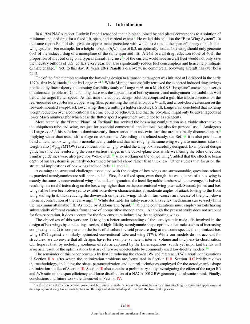
(a) box wing (BW) (b) tube-and-wing (TW)Figure 1: Outer mold line of the BW and reference TW regional jets.

II. Problem Setup and MethodologyII.A. Initial GeometryThe BW aircraft studied in this work is intended to perform a regional mission consisting of carrying 100 passengersand 3 crew members over 926 km (∼ 500 nm) at Mach 0.78 and an altitude of 10.5 km (∼ 35,000 ft). The referenceTW aircraft is the Bombardier CRJ1000 NextGen.15 The initial outer mold line geometries of both configurations areshown in Fig. 1. Compared to the TW, the BW has wider fuselage cross-sections which allows for the installation ofthe structurally efficient twin-fins mentioned in Section I. The wider fuselage also allows for a 3-2 seating arrangement(as opposed to 2-2 for the TW); hence, for the same capacity the BW is also shorter: 34.31m compared to 38.77m forthe TW. For a given wing span and sweep, the shorter fuselage allows the longitudinal spread of the top and bottomwings to be increased without resorting to overly swept-back tip fins. Maximizing the distance between the two wingshelps keep the center of gravity in the middle which improves elevator effectiveness.6

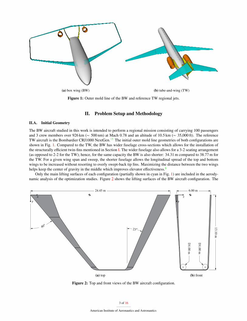
Only the main lifting surfaces of each configuration (partially shown in cyan in Fig. 1) are included in the aerody-namic analysis of the optimization studies. Figure 2 shows the lifting surfaces of the BW aircraft configuration. The

24.45 m

(a) top

13.10 m

6.00 m

D1.00 m

D1.00 m

(b) frontFigure 2: Top and front views of the BW aircraft configuration.


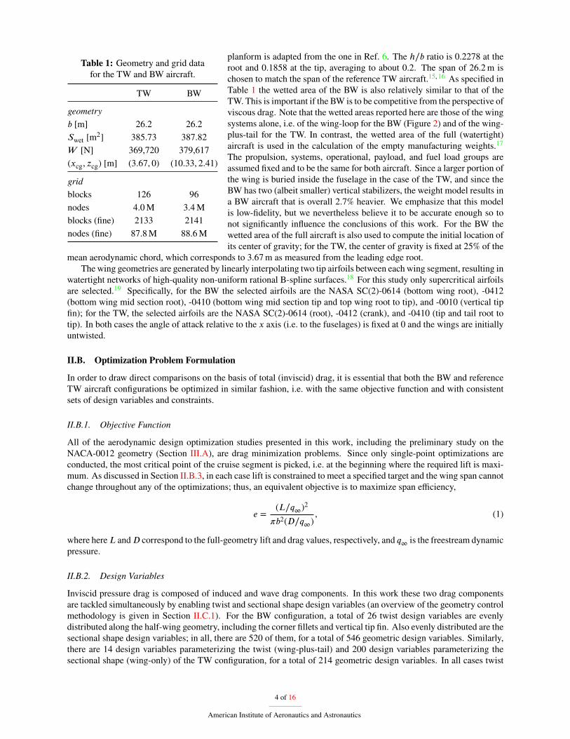
Table 1: Geometry and grid datafor the TW and BW aircraft.

TW BWgeometryb [m] 26.2 26.2Swet [m2] 385.73 387.82W [N] 369,720 379,617(xcg, zcg) [m] (3.67, 0) (10.33, 2.41)gridblocks 126 96nodes 4.0M 3.4Mblocks (fine) 2133 2141nodes (fine) 87.8M 88.6M

planform is adapted from the one in Ref. 6. The ℎ∕b ratio is 0.2278 at theroot and 0.1858 at the tip, averaging to about 0.2. The span of 26.2m ischosen to match the span of the reference TW aircraft.15,16 As specified inTable 1 the wetted area of the BW is also relatively similar to that of theTW. This is important if the BW is to be competitive from the perspective ofviscous drag. Note that the wetted areas reported here are those of the wingsystems alone, i.e. of the wing-loop for the BW (Figure 2) and of the wing-plus-tail for the TW. In contrast, the wetted area of the full (watertight)aircraft is used in the calculation of the empty manufacturing weights.17The propulsion, systems, operational, payload, and fuel load groups areassumed fixed and to be the same for both aircraft. Since a larger portion ofthe wing is buried inside the fuselage in the case of the TW, and since theBW has two (albeit smaller) vertical stabilizers, the weight model results ina BW aircraft that is overall 2.7% heavier. We emphasize that this modelis low-fidelity, but we nevertheless believe it to be accurate enough so tonot significantly influence the conclusions of this work. For the BW thewetted area of the full aircraft is also used to compute the initial location ofits center of gravity; for the TW, the center of gravity is fixed at 25% of the

mean aerodynamic chord, which corresponds to 3.67m as measured from the leading edge root.The wing geometries are generated by linearly interpolating two tip airfoils between each wing segment, resulting in

watertight networks of high-quality non-uniform rational B-spline surfaces.18 For this study only supercritical airfoilsare selected.19 Specifically, for the BW the selected airfoils are the NASA SC(2)-0614 (bottom wing root), -0412(bottom wing mid section root), -0410 (bottom wing mid section tip and top wing root to tip), and -0010 (vertical tipfin); for the TW, the selected airfoils are the NASA SC(2)-0614 (root), -0412 (crank), and -0410 (tip and tail root totip). In both cases the angle of attack relative to the x axis (i.e. to the fuselages) is fixed at 0 and the wings are initiallyuntwisted.

II.B. Optimization Problem FormulationIn order to draw direct comparisons on the basis of total (inviscid) drag, it is essential that both the BW and referenceTW aircraft configurations be optimized in similar fashion, i.e. with the same objective function and with consistentsets of design variables and constraints.

II.B.1. Objective Function

All of the aerodynamic design optimization studies presented in this work, including the preliminary study on theNACA-0012 geometry (Section III.A), are drag minimization problems. Since only single-point optimizations areconducted, the most critical point of the cruise segment is picked, i.e. at the beginning where the required lift is maxi-mum. As discussed in Section II.B.3, in each case lift is constrained to meet a specified target and the wing span cannotchange throughout any of the optimizations; thus, an equivalent objective is to maximize span efficiency,

e =(L∕q∞)2

�b2(D∕q∞), (1)

where hereL andD correspond to the full-geometry lift and drag values, respectively, and q∞ is the freestream dynamicpressure.

II.B.2. Design Variables

Inviscid pressure drag is composed of induced and wave drag components. In this work these two drag componentsare tackled simultaneously by enabling twist and sectional shape design variables (an overview of the geometry controlmethodology is given in Section II.C.1). For the BW configuration, a total of 26 twist design variables are evenlydistributed along the half-wing geometry, including the corner fillets and vertical tip fin. Also evenly distributed are thesectional shape design variables; in all, there are 520 of them, for a total of 546 geometric design variables. Similarly,there are 14 design variables parameterizing the twist (wing-plus-tail) and 200 design variables parameterizing thesectional shape (wing-only) of the TW configuration, for a total of 214 geometric design variables. In all cases twist


is applied about the leading edge of the wing segments. For both configurations the twist design variables include theangle of incidence (relative to the x axis) of the wings’ root sections.

For Study 5 only (Section III.F) the leading-edge sweep angles of the top and bottom wings are design variables.The same design variables control the sweep of the tip fin while maintaining smooth corner fillets.

Finally, given the conceptual nature of the design problem and in particular the low-fidelity of the weight andbalance model, the longitudinal location of the center of gravity, xcg, can also be chosen as a design variable. Whendoing so it is however important to enforce a proper longitudinal stability constraint, as discussed next.

II.B.3. Constraints

A high-fidelity aerodynamic optimization problem must be carefully constrained in order to retrieve realistic shapes.For example, if unconstrained, a single-point Euler-based optimization would result in wings with minimal internalvolume and razor-thin leading edges. To address the first difficulty, an internal volume inequality constraint with alower bound of 95% of the initial value is enforced for all cases. To address the second difficulty, the wing sections areconstrained to maintain at least 60% of their original thickness at any chordwise location. For example, a wing sectionthat is initially 10% thick cannot become less than 6% thick. Finally, twist is linearly interpolated between the two tipsections of any given wing segment, a measure that reduces the development of overly wavy surfaces in the spanwisedirection and that fortunately has a minimal impact on drag.

As already mentioned in Section II.B.1, lift is constrained to a target value for all drag minimization studies. Thetarget value is set to be equal to the aircraft weight at the beginning of the cruise segment. For the half-geometry BWaircraft this value corresponds to L∕q∞ = 19.6m2. When comparing the performance of different aircraft configura-tions it is also important that each configuration be trimmed at its design point. This is achieved here by constrainingthe optimizer to achieve a pitching moment,My, of 0 about the center of gravity. However, if the location of the centerof gravity is poorly chosen, then a configuration may be overly penalized from this trim constraint. Activating xcg as adesign variable can help, but if such is the case then additional preventive measures must also be taken, otherwise theoptimizer will simply move xcg such that the constraint is satisfied. In general, moving the center of gravity aft reduceslongitudinal stability, hence there is a trade-off between xcg, trim, and stability. In this work we constrain longitudinalstability by forcing the center of gravity to remain at least 5% of the root-chord length ahead of the neutral point, xnp,i.e.

xnp − xcg = −(My∕q∞)�(L∕q∞)�

≥ 0.05c, (2)

where the � subscript denotes the partial derivative with respect to the angle of attack. FollowingMader andMartins,20these partials are evaluated using a first-order finite-difference approximation. Round-off errors can be minimized bychoosing a relatively large step size (0.001◦) while keeping the truncation errors within acceptable bounds, since boththe pitching moment and lift are relatively linear in � for the flow regimes considered here.

The coupling between the aerodynamic and structural forces is strong in wing design, especially in the case ofthe BW due to its unique snap-buckling and post-critical patterns.12 While a full aerostructural shape optimization21is beyond the scope of this work, here we consider the center-plane bending moment as a surrogate for a structuralmodel.22 Specifically, the x-directional moment, Mx, about the center of gravity is constrained to be no more than80% of the bending moment generated by the same configuration optimized without a bending moment constraint.For example, in the case of the TW, the lower bound is 80% of the bending moment generated by an elliptical liftdistribution. Note that unlike the TW case, the vertical location of the center of gravity, zcg, of the BW cannot beneglected since the tip fin can generate significant side-forces. An alternative would be to apply the bending momentconstraint to the top and bottom wings separately, although at the time of writing it is unclear if this approach wouldbe preferable.

II.C. Optimization AlgorithmThe objective function, design variables, and constraints described in Section II.B are computed by state-of-the-art op-timization software collectively known as Jetstream. Many of the core components of the methodology are thoroughlydescribed and verified in Ref. 23; thus, only a brief summary is given here.

II.C.1. Geometry Parameterization and Mesh Movement

The twist, sectional shape, and planform design variables are handled by a geometry control system built around free-form and axial deformation.24 Whereas the free-form deformation volumes (modeled as B-spline volumes) are effective


at local control such as twist and sectional shape changes, the axial curves (also modeled with B-spline technology)are effective at global control such as planform changes. In general each wing segment, including the corner fillets andvertical tip fin of the BW, is assigned a single free-form deformation volume that stretches between the wing segment’stip sections. The same free-form deformation volumes are positioned such that they overlap at the tip sections. Sinceall free-form deformation volumes are linear in the vertical directionb and cubic in the other two directions, the overallwing shape is thus parameterized by piecewise-cubic polynomials in the chordwise and spanwise directions.

Following an update in the geometric design variables, the computational grid that surrounds the geometry mustalso deform. This is accomplished by an efficient two-level approach that models the grid as a linear elastic solid.23,24

II.C.2. Flow Solver

With the computational grid conforming to the deformed geometry, the aerodynamic functionals are evaluated basedon the solution of the steady Euler equations, discretized here with second-order accurate finite-difference operators.The solution in the vicinity of shocks is stabilized by a pressure sensor mechanism involving both fourth- and second-difference scalar dissipation. The vector of nonlinear residuals is converged to a relative tolerance of 10−12 by anefficient parallel Newton-Krylov solver. Further details regarding the flow solver are available in Ref. 25.

Basic information on the size of the computational grids used for the optimization studies is given in Table 1. Whilethe coarse grids are fine enough for the optimizer to capture the physics and thus correctly shape the geometry, they arenevertheless too coarse to accurately predict drag. Therefore, we perform flow analyses on fine grids before and afteroptimization.

II.C.3. Optimizer

Jetstream relies on the gradient-based package SNOPT26 to drive the optimization process. SNOPT uses sequentialquadratic programming and is capable of handling thousands of design variables and constraints. To achieve deep con-vergence it is however necessary that the gradients of the functionals with respect to the design variables be accuratelydefined. For nonlinear constraints that do not depend on the flow, such as the internal volume, the gradients are mostlyhand-differentiated. Otherwise, they are computed through the discrete-adjoint method.23,24

III. Aerodynamic Design Optimization StudiesWe now present five drag minimization studies that investigate the effect of particular combinations of design

variables and constraints on the aerodynamic performance of the transonic BW configuration. A summary of eachstudy is given in Table 2. In each case an equivalent set of design variables and constraints is used to optimize thereference TW configuration. This is with the exception of Study 5, for which the sweep design variables are onlyactivated on the BW configuration. For all other cases the planform of both configurations is fixed due to the absenceof off-design, structural, and viscous models.

Sections III.B to III.F are each assigned one optimization study. In order to gain insight and confidence we firstpresent a preliminary study on a simple NACA-0012 BW geometry. A similar study is proposed as benchmark to the2015 AIAA Aerodynamic Design Optimization Discussion Groupc.27

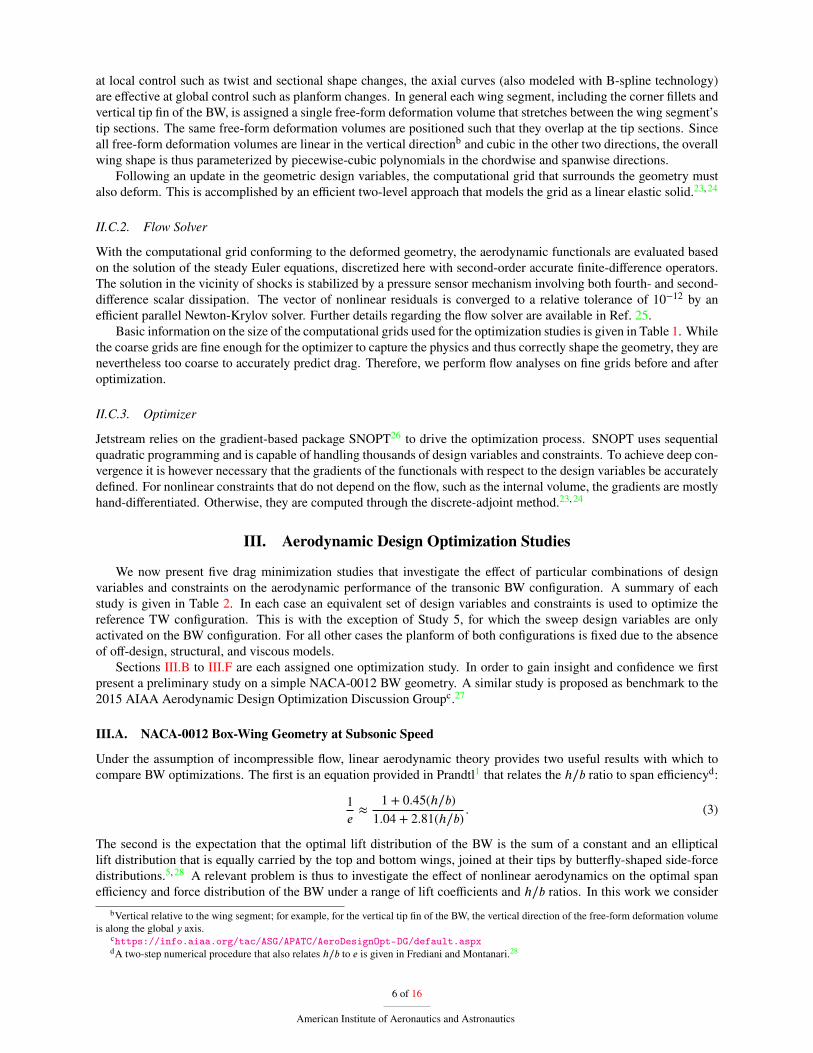
III.A. NACA-0012 Box-Wing Geometry at Subsonic SpeedUnder the assumption of incompressible flow, linear aerodynamic theory provides two useful results with which tocompare BW optimizations. The first is an equation provided in Prandtl1 that relates the ℎ∕b ratio to span efficiencyd:

1e≈

1 + 0.45(ℎ∕b)1.04 + 2.81(ℎ∕b)

. (3)

The second is the expectation that the optimal lift distribution of the BW is the sum of a constant and an ellipticallift distribution that is equally carried by the top and bottom wings, joined at their tips by butterfly-shaped side-forcedistributions.5,28 A relevant problem is thus to investigate the effect of nonlinear aerodynamics on the optimal spanefficiency and force distribution of the BW under a range of lift coefficients and ℎ∕b ratios. In this work we consider

bVertical relative to the wing segment; for example, for the vertical tip fin of the BW, the vertical direction of the free-form deformation volumeis along the global y axis.

chttps://info.aiaa.org/tac/ASG/APATC/AeroDesignOpt-DG/default.aspxdA two-step numerical procedure that also relates ℎ∕b to e is given in Frediani and Montanari.28


https://info.aiaa.org/tac/ASG/APATC/AeroDesignOpt-DG/default.aspx

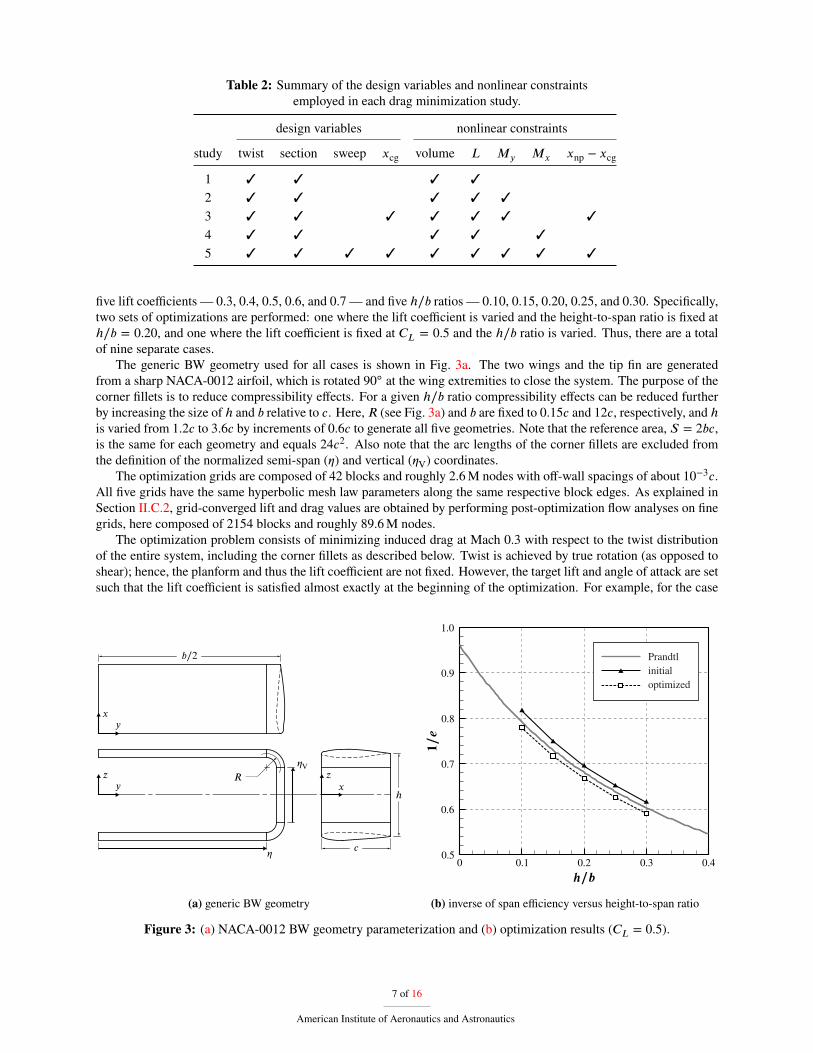
Table 2: Summary of the design variables and nonlinear constraintsemployed in each drag minimization study.

design variables nonlinear constraintsstudy twist section sweep xcg volume L My Mx xnp − xcg1 ✓ ✓ ✓ ✓

2 ✓ ✓ ✓ ✓ ✓

3 ✓ ✓ ✓ ✓ ✓ ✓ ✓

4 ✓ ✓ ✓ ✓ ✓

5 ✓ ✓ ✓ ✓ ✓ ✓ ✓ ✓ ✓

five lift coefficients — 0.3, 0.4, 0.5, 0.6, and 0.7 — and five ℎ∕b ratios — 0.10, 0.15, 0.20, 0.25, and 0.30. Specifically,two sets of optimizations are performed: one where the lift coefficient is varied and the height-to-span ratio is fixed atℎ∕b = 0.20, and one where the lift coefficient is fixed at CL = 0.5 and the ℎ∕b ratio is varied. Thus, there are a totalof nine separate cases.

The generic BW geometry used for all cases is shown in Fig. 3a. The two wings and the tip fin are generatedfrom a sharp NACA-0012 airfoil, which is rotated 90◦ at the wing extremities to close the system. The purpose of thecorner fillets is to reduce compressibility effects. For a given ℎ∕b ratio compressibility effects can be reduced furtherby increasing the size of ℎ and b relative to c. Here,R (see Fig. 3a) and b are fixed to 0.15c and 12c, respectively, and ℎis varied from 1.2c to 3.6c by increments of 0.6c to generate all five geometries. Note that the reference area, S = 2bc,is the same for each geometry and equals 24c2. Also note that the arc lengths of the corner fillets are excluded fromthe definition of the normalized semi-span (�) and vertical (�V) coordinates.The optimization grids are composed of 42 blocks and roughly 2.6M nodes with off-wall spacings of about 10−3c.All five grids have the same hyperbolic mesh law parameters along the same respective block edges. As explained inSection II.C.2, grid-converged lift and drag values are obtained by performing post-optimization flow analyses on finegrids, here composed of 2154 blocks and roughly 89.6M nodes.

The optimization problem consists of minimizing induced drag at Mach 0.3 with respect to the twist distributionof the entire system, including the corner fillets as described below. Twist is achieved by true rotation (as opposed toshear); hence, the planform and thus the lift coefficient are not fixed. However, the target lift and angle of attack are setsuch that the lift coefficient is satisfied almost exactly at the beginning of the optimization. For example, for the case

(a) generic BW geometry

Prandtl

optimizedinitial

(b) inverse of span efficiency versus height-to-span ratioFigure 3: (a) NACA-0012 BW geometry parameterization and (b) optimization results (CL = 0.5).


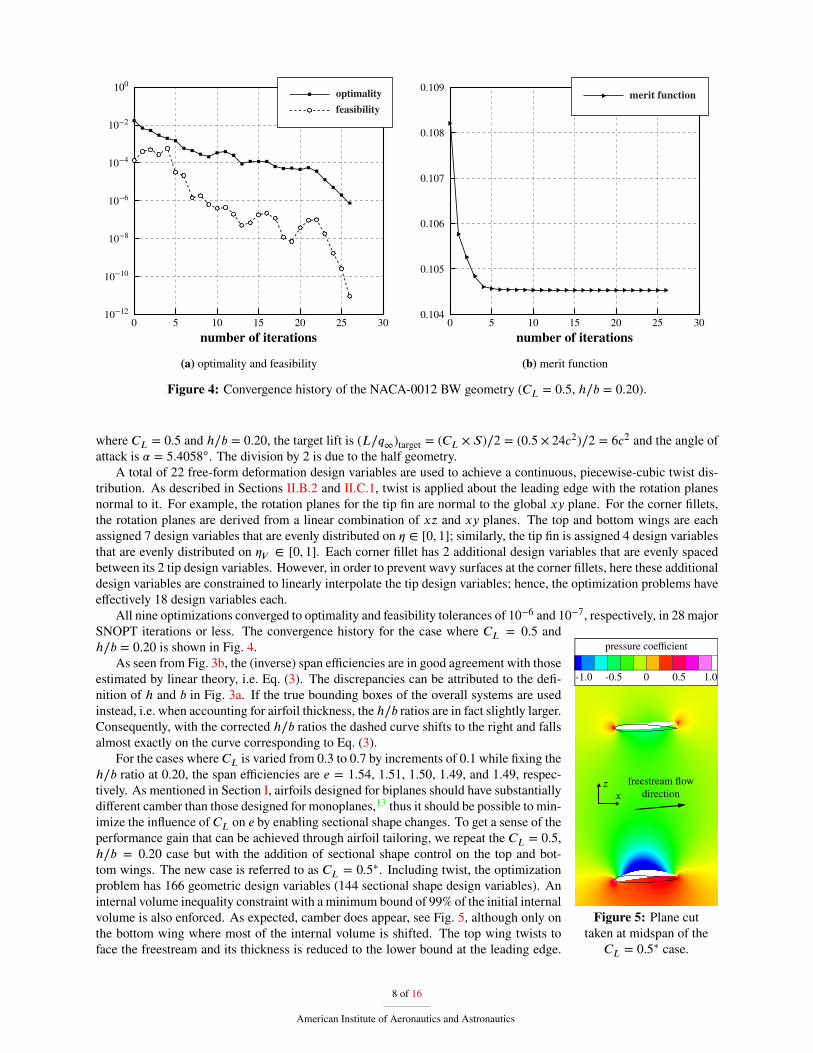
optimalityfeasibility

0 5 10 15 20 25 30number of iterations

(a) optimality and feasibility

0 5 10 15 20 25 300.104

0.105

0.106

0.107

0.108

0.109

number of iterations

merit function

(b) merit functionFigure 4: Convergence history of the NACA-0012 BW geometry (CL = 0.5, ℎ∕b = 0.20).

where CL = 0.5 and ℎ∕b = 0.20, the target lift is (L∕q∞)target = (CL × S)∕2 = (0.5 × 24c2)∕2 = 6c2 and the angle ofattack is � = 5.4058◦. The division by 2 is due to the half geometry.A total of 22 free-form deformation design variables are used to achieve a continuous, piecewise-cubic twist dis-

tribution. As described in Sections II.B.2 and II.C.1, twist is applied about the leading edge with the rotation planesnormal to it. For example, the rotation planes for the tip fin are normal to the global xy plane. For the corner fillets,the rotation planes are derived from a linear combination of xz and xy planes. The top and bottom wings are eachassigned 7 design variables that are evenly distributed on � ∈ [0, 1]; similarly, the tip fin is assigned 4 design variablesthat are evenly distributed on �V ∈ [0, 1]. Each corner fillet has 2 additional design variables that are evenly spacedbetween its 2 tip design variables. However, in order to prevent wavy surfaces at the corner fillets, here these additionaldesign variables are constrained to linearly interpolate the tip design variables; hence, the optimization problems haveeffectively 18 design variables each.

All nine optimizations converged to optimality and feasibility tolerances of 10−6 and 10−7, respectively, in 28 major

-1.0 -0.5 0 0.5 1.0

pressure coefficient

freestream flowdirection

Figure 5: Plane cuttaken at midspan of the

CL = 0.5∗ case.

SNOPT iterations or less. The convergence history for the case where CL = 0.5 andℎ∕b = 0.20 is shown in Fig. 4.

As seen from Fig. 3b, the (inverse) span efficiencies are in good agreement with thoseestimated by linear theory, i.e. Eq. (3). The discrepancies can be attributed to the defi-nition of ℎ and b in Fig. 3a. If the true bounding boxes of the overall systems are usedinstead, i.e. when accounting for airfoil thickness, the ℎ∕b ratios are in fact slightly larger.Consequently, with the corrected ℎ∕b ratios the dashed curve shifts to the right and fallsalmost exactly on the curve corresponding to Eq. (3).

For the cases where CL is varied from 0.3 to 0.7 by increments of 0.1 while fixing theℎ∕b ratio at 0.20, the span efficiencies are e = 1.54, 1.51, 1.50, 1.49, and 1.49, respec-tively. As mentioned in Section I, airfoils designed for biplanes should have substantiallydifferent camber than those designed for monoplanes,13 thus it should be possible to min-imize the influence of CL on e by enabling sectional shape changes. To get a sense of theperformance gain that can be achieved through airfoil tailoring, we repeat the CL = 0.5,ℎ∕b = 0.20 case but with the addition of sectional shape control on the top and bot-tom wings. The new case is referred to as CL = 0.5∗. Including twist, the optimizationproblem has 166 geometric design variables (144 sectional shape design variables). Aninternal volume inequality constraint with a minimum bound of 99% of the initial internalvolume is also enforced. As expected, camber does appear, see Fig. 5, although only onthe bottom wing where most of the internal volume is shifted. The top wing twists toface the freestream and its thickness is reduced to the lower bound at the leading edge.


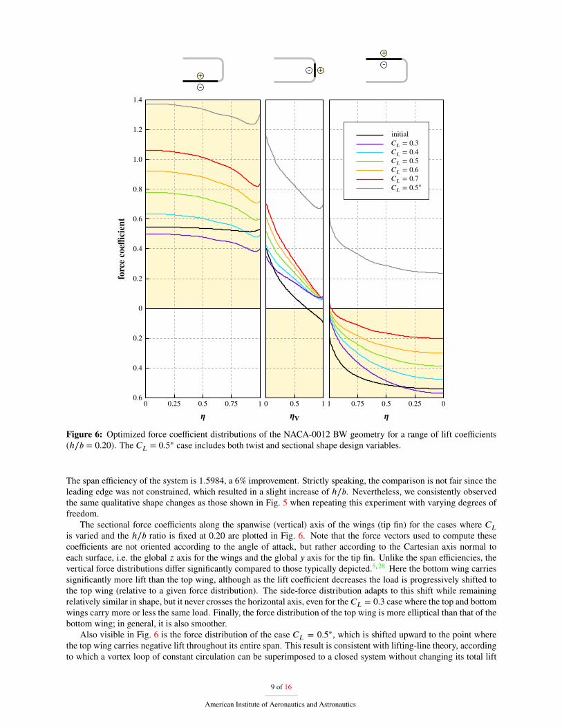
1.4

0

0.6 0 1 0 1 1 00.25 0.5 0.75 0.5 0.75 0.5 0.25

0.4

0.2

0.2

0.4

0.6

0.8

1.0

1.2fo

rce c

oeffi

cient

initial

Figure 6: Optimized force coefficient distributions of the NACA-0012 BW geometry for a range of lift coefficients(ℎ∕b = 0.20). The CL = 0.5∗ case includes both twist and sectional shape design variables.

The span efficiency of the system is 1.5984, a 6% improvement. Strictly speaking, the comparison is not fair since theleading edge was not constrained, which resulted in a slight increase of ℎ∕b. Nevertheless, we consistently observedthe same qualitative shape changes as those shown in Fig. 5 when repeating this experiment with varying degrees offreedom.

The sectional force coefficients along the spanwise (vertical) axis of the wings (tip fin) for the cases where CLis varied and the ℎ∕b ratio is fixed at 0.20 are plotted in Fig. 6. Note that the force vectors used to compute thesecoefficients are not oriented according to the angle of attack, but rather according to the Cartesian axis normal toeach surface, i.e. the global z axis for the wings and the global y axis for the tip fin. Unlike the span efficiencies, thevertical force distributions differ significantly compared to those typically depicted.5,28 Here the bottom wing carriessignificantly more lift than the top wing, although as the lift coefficient decreases the load is progressively shifted tothe top wing (relative to a given force distribution). The side-force distribution adapts to this shift while remainingrelatively similar in shape, but it never crosses the horizontal axis, even for the CL = 0.3 case where the top and bottomwings carry more or less the same load. Finally, the force distribution of the top wing is more elliptical than that of thebottom wing; in general, it is also smoother.

Also visible in Fig. 6 is the force distribution of the case CL = 0.5∗, which is shifted upward to the point wherethe top wing carries negative lift throughout its entire span. This result is consistent with lifting-line theory, accordingto which a vortex loop of constant circulation can be superimposed to a closed system without changing its total lift


bottom wingtip fintop wing

twist

(deg

rees

)

twist (degrees)

0 0.25 0.5 0.75 1 0

0.25

0.5

0.75

1

-3

-1.5

0

1.5

3-3 -1.5 0 1.5 3

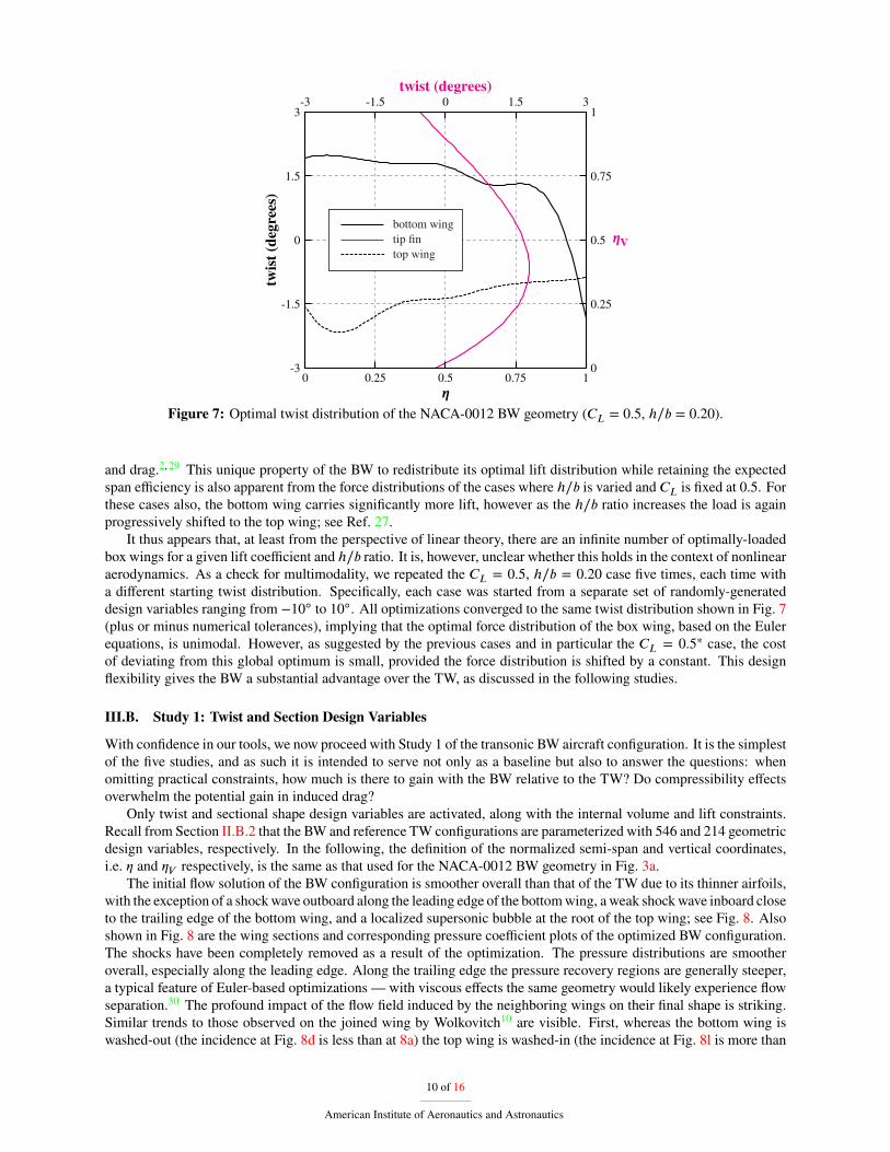
Figure 7: Optimal twist distribution of the NACA-0012 BW geometry (CL = 0.5, ℎ∕b = 0.20).

and drag.2,29 This unique property of the BW to redistribute its optimal lift distribution while retaining the expectedspan efficiency is also apparent from the force distributions of the cases where ℎ∕b is varied and CL is fixed at 0.5. Forthese cases also, the bottom wing carries significantly more lift, however as the ℎ∕b ratio increases the load is againprogressively shifted to the top wing; see Ref. 27.

It thus appears that, at least from the perspective of linear theory, there are an infinite number of optimally-loadedbox wings for a given lift coefficient and ℎ∕b ratio. It is, however, unclear whether this holds in the context of nonlinearaerodynamics. As a check for multimodality, we repeated the CL = 0.5, ℎ∕b = 0.20 case five times, each time witha different starting twist distribution. Specifically, each case was started from a separate set of randomly-generateddesign variables ranging from −10◦ to 10◦. All optimizations converged to the same twist distribution shown in Fig. 7(plus or minus numerical tolerances), implying that the optimal force distribution of the box wing, based on the Eulerequations, is unimodal. However, as suggested by the previous cases and in particular the CL = 0.5∗ case, the costof deviating from this global optimum is small, provided the force distribution is shifted by a constant. This designflexibility gives the BW a substantial advantage over the TW, as discussed in the following studies.

III.B. Study 1: Twist and Section Design VariablesWith confidence in our tools, we now proceed with Study 1 of the transonic BW aircraft configuration. It is the simplestof the five studies, and as such it is intended to serve not only as a baseline but also to answer the questions: whenomitting practical constraints, how much is there to gain with the BW relative to the TW? Do compressibility effectsoverwhelm the potential gain in induced drag?

Only twist and sectional shape design variables are activated, along with the internal volume and lift constraints.Recall from Section II.B.2 that the BW and reference TW configurations are parameterized with 546 and 214 geometricdesign variables, respectively. In the following, the definition of the normalized semi-span and vertical coordinates,i.e. � and �V respectively, is the same as that used for the NACA-0012 BW geometry in Fig. 3a.

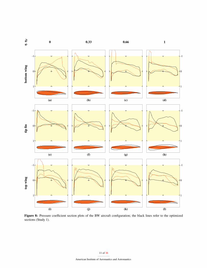
The initial flow solution of the BW configuration is smoother overall than that of the TW due to its thinner airfoils,with the exception of a shockwave outboard along the leading edge of the bottomwing, aweak shockwave inboard closeto the trailing edge of the bottom wing, and a localized supersonic bubble at the root of the top wing; see Fig. 8. Alsoshown in Fig. 8 are the wing sections and corresponding pressure coefficient plots of the optimized BW configuration.The shocks have been completely removed as a result of the optimization. The pressure distributions are smootheroverall, especially along the leading edge. Along the trailing edge the pressure recovery regions are generally steeper,a typical feature of Euler-based optimizations — with viscous effects the same geometry would likely experience flowseparation.30 The profound impact of the flow field induced by the neighboring wings on their final shape is striking.Similar trends to those observed on the joined wing by Wolkovitch10 are visible. First, whereas the bottom wing iswashed-out (the incidence at Fig. 8d is less than at 8a) the top wing is washed-in (the incidence at Fig. 8l is more than


�,� V 0 0.33 0.66 1

botto

mwing

-1

0

1

(a) (b) (c)

-1

0

1

(d)

tipfin

-1

0

1

(e) (f) (g)

-1

0

1

(h)

topwing

-1

0

1

(i) (j) (k)

-1

0

1

(l)

Figure 8: Pressure coefficient section plots of the BW aircraft configuration; the black lines refer to the optimizedsections (Study 1).


0.5

0.2

0.5 0 1 0 1 1 00.25 0.5 0.75 0.5 0.75 0.5 0.25

0.4

0.3

0.1

0

0.1

0.2

0.3

0.4fo

rce c

oeffi

cient

initialstudy 1study 2study 3study 4study 5

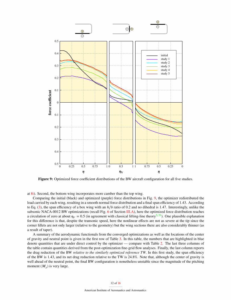
Figure 9: Optimized force coefficient distributions of the BW aircraft configuration for all five studies.

at 8i). Second, the bottom wing incorporates more camber than the top wing.Comparing the initial (black) and optimized (purple) force distributions in Fig. 9, the optimizer redistributed the

load carried by each wing, resulting in a smooth normal force distribution and a final span efficiency of 1.43. Accordingto Eq. (3), the span efficiency of a box wing with an ℎ∕b ratio of 0.2 and no dihedral is 1.47. Interestingly, unlike thesubsonic NACA-0012 BW optimizations (recall Fig. 6 of Section III.A), here the optimized force distribution reachesa circulation of zero at about �V = 0.5 (in agreement with classical lifting-line theory5,28). One plausible explanationfor this difference is that, despite the transonic speed, here the nonlinear effects are not as severe at the tip since thecorner fillets are not only larger (relative to the geometry) but the wing sections there are also considerably thinner (asa result of taper).

A summary of the aerodynamic functionals from the converged optimizations as well as the locations of the centerof gravity and neutral point is given in the first row of Table 3. In this table, the numbers that are highlighted in bluedenote quantities that are under direct control by the optimizer — compare with Table 2. The last three columns ofthe table contain quantities derived from the post-optimization fine-grid flow analyses. Finally, the last column reportsthe drag reduction of the BW relative to the similarly optimized reference TW. In this first study, the span efficiencyof the BW is 1.43, and its net drag reduction relative to the TW is 24.8%. Note that, although the center of gravity iswell ahead of the neutral point, the final BW configuration is nonetheless unstable since the magnitude of the pitchingmoment (My) is very large.


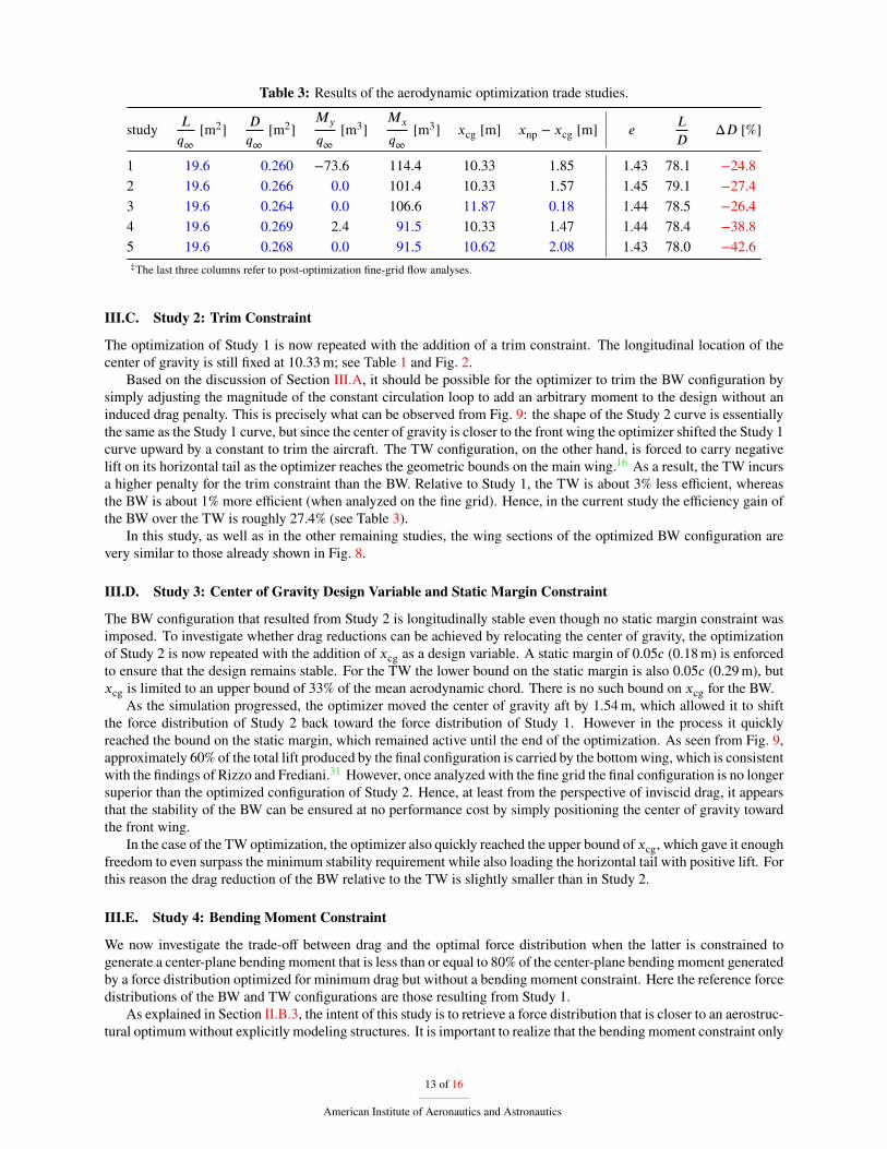
Table 3: Results of the aerodynamic optimization trade studies.

study Lq∞

[m2] Dq∞

[m2] My

q∞[m3] Mx

q∞[m3] xcg [m] xnp − xcg [m] e L

DΔD [%]

1 19.6 0.260 −73.6 114.4 10.33 1.85 1.43 78.1 −24.82 19.6 0.266 0.0 101.4 10.33 1.57 1.45 79.1 −27.43 19.6 0.264 0.0 106.6 11.87 0.18 1.44 78.5 −26.44 19.6 0.269 2.4 91.5 10.33 1.47 1.44 78.4 −38.85 19.6 0.268 0.0 91.5 10.62 2.08 1.43 78.0 −42.6‡The last three columns refer to post-optimization fine-grid flow analyses.

III.C. Study 2: Trim ConstraintThe optimization of Study 1 is now repeated with the addition of a trim constraint. The longitudinal location of thecenter of gravity is still fixed at 10.33m; see Table 1 and Fig. 2.

Based on the discussion of Section III.A, it should be possible for the optimizer to trim the BW configuration bysimply adjusting the magnitude of the constant circulation loop to add an arbitrary moment to the design without aninduced drag penalty. This is precisely what can be observed from Fig. 9: the shape of the Study 2 curve is essentiallythe same as the Study 1 curve, but since the center of gravity is closer to the front wing the optimizer shifted the Study 1curve upward by a constant to trim the aircraft. The TW configuration, on the other hand, is forced to carry negativelift on its horizontal tail as the optimizer reaches the geometric bounds on the main wing.16 As a result, the TW incursa higher penalty for the trim constraint than the BW. Relative to Study 1, the TW is about 3% less efficient, whereasthe BW is about 1% more efficient (when analyzed on the fine grid). Hence, in the current study the efficiency gain ofthe BW over the TW is roughly 27.4% (see Table 3).

In this study, as well as in the other remaining studies, the wing sections of the optimized BW configuration arevery similar to those already shown in Fig. 8.

III.D. Study 3: Center of Gravity Design Variable and Static Margin ConstraintThe BW configuration that resulted from Study 2 is longitudinally stable even though no static margin constraint wasimposed. To investigate whether drag reductions can be achieved by relocating the center of gravity, the optimizationof Study 2 is now repeated with the addition of xcg as a design variable. A static margin of 0.05c (0.18m) is enforcedto ensure that the design remains stable. For the TW the lower bound on the static margin is also 0.05c (0.29m), butxcg is limited to an upper bound of 33% of the mean aerodynamic chord. There is no such bound on xcg for the BW.

As the simulation progressed, the optimizer moved the center of gravity aft by 1.54m, which allowed it to shiftthe force distribution of Study 2 back toward the force distribution of Study 1. However in the process it quicklyreached the bound on the static margin, which remained active until the end of the optimization. As seen from Fig. 9,approximately 60% of the total lift produced by the final configuration is carried by the bottomwing, which is consistentwith the findings of Rizzo and Frediani.31 However, once analyzed with the fine grid the final configuration is no longersuperior than the optimized configuration of Study 2. Hence, at least from the perspective of inviscid drag, it appearsthat the stability of the BW can be ensured at no performance cost by simply positioning the center of gravity towardthe front wing.

In the case of the TW optimization, the optimizer also quickly reached the upper bound of xcg, which gave it enoughfreedom to even surpass the minimum stability requirement while also loading the horizontal tail with positive lift. Forthis reason the drag reduction of the BW relative to the TW is slightly smaller than in Study 2.

III.E. Study 4: Bending Moment ConstraintWe now investigate the trade-off between drag and the optimal force distribution when the latter is constrained togenerate a center-plane bending moment that is less than or equal to 80% of the center-plane bending moment generatedby a force distribution optimized for minimum drag but without a bending moment constraint. Here the reference forcedistributions of the BW and TW configurations are those resulting from Study 1.

As explained in Section II.B.3, the intent of this study is to retrieve a force distribution that is closer to an aerostruc-tural optimumwithout explicitly modeling structures. It is important to realize that the bending moment constraint only


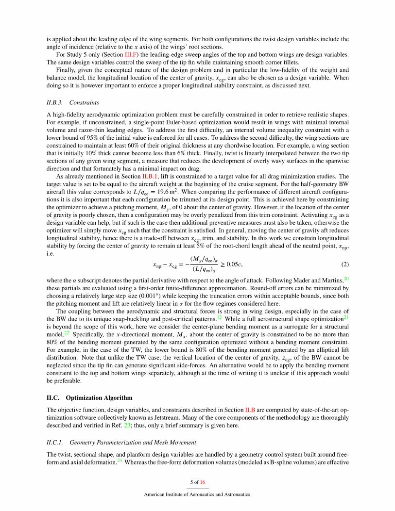
Y

ZX

normalizedvertical (Z)componentof momentum

(a) initialY

ZX

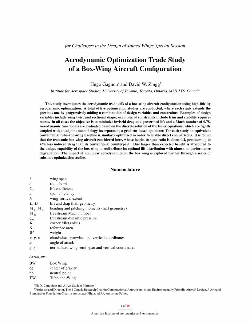
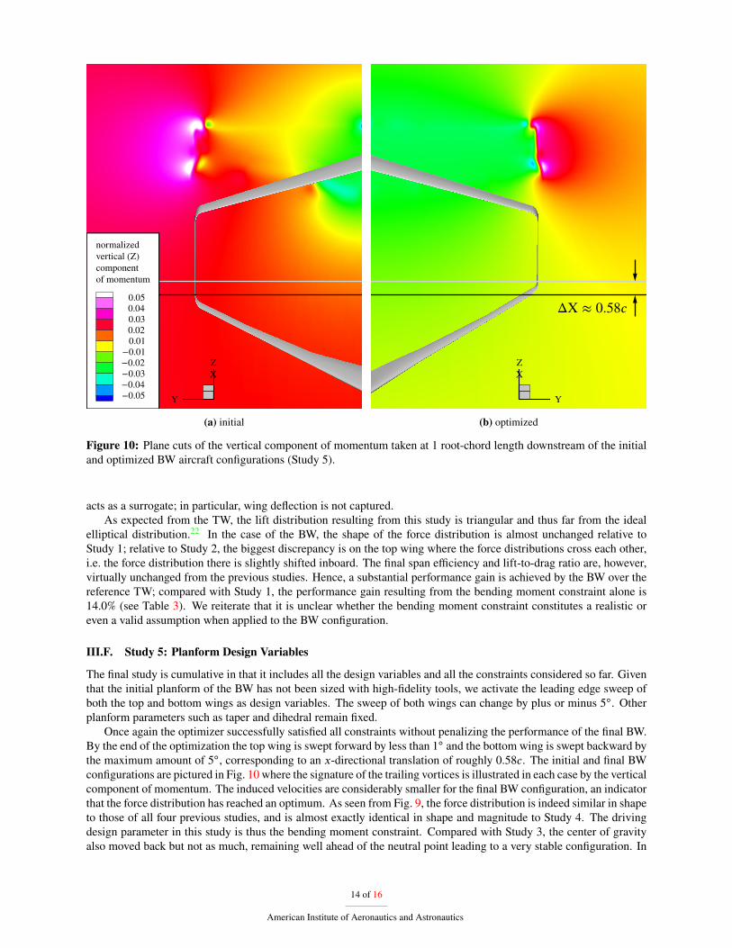
(b) optimizedFigure 10: Plane cuts of the vertical component of momentum taken at 1 root-chord length downstream of the initialand optimized BW aircraft configurations (Study 5).

acts as a surrogate; in particular, wing deflection is not captured.As expected from the TW, the lift distribution resulting from this study is triangular and thus far from the ideal

elliptical distribution.22 In the case of the BW, the shape of the force distribution is almost unchanged relative toStudy 1; relative to Study 2, the biggest discrepancy is on the top wing where the force distributions cross each other,i.e. the force distribution there is slightly shifted inboard. The final span efficiency and lift-to-drag ratio are, however,virtually unchanged from the previous studies. Hence, a substantial performance gain is achieved by the BW over thereference TW; compared with Study 1, the performance gain resulting from the bending moment constraint alone is14.0% (see Table 3). We reiterate that it is unclear whether the bending moment constraint constitutes a realistic oreven a valid assumption when applied to the BW configuration.

III.F. Study 5: Planform Design VariablesThe final study is cumulative in that it includes all the design variables and all the constraints considered so far. Giventhat the initial planform of the BW has not been sized with high-fidelity tools, we activate the leading edge sweep ofboth the top and bottom wings as design variables. The sweep of both wings can change by plus or minus 5◦. Otherplanform parameters such as taper and dihedral remain fixed.

Once again the optimizer successfully satisfied all constraints without penalizing the performance of the final BW.By the end of the optimization the top wing is swept forward by less than 1◦ and the bottom wing is swept backward bythe maximum amount of 5◦, corresponding to an x-directional translation of roughly 0.58c. The initial and final BWconfigurations are pictured in Fig. 10 where the signature of the trailing vortices is illustrated in each case by the verticalcomponent of momentum. The induced velocities are considerably smaller for the final BW configuration, an indicatorthat the force distribution has reached an optimum. As seen from Fig. 9, the force distribution is indeed similar in shapeto those of all four previous studies, and is almost exactly identical in shape and magnitude to Study 4. The drivingdesign parameter in this study is thus the bending moment constraint. Compared with Study 3, the center of gravityalso moved back but not as much, remaining well ahead of the neutral point leading to a very stable configuration. In


the case of reference TW, the optimizer could also satisfy all constraints but at the expense of producing 42.6% moredrag than the BW.

IV. Conclusions and Future WorkThis work studied the aerodynamic trade-offs of a transonic box-wing regional jet configuration using high-fidelity

computational fluid dynamics and optimization.The influence of nonlinear physics on the aerodynamics of the box wing was first investigated by optimizing a

simple NACA-0012 box-wing geometry at subsonic speed under a range of lift coefficients and height-to-span ratios.While the resulting span efficiencies are in excellent agreement with those estimated by linear theory, the optimal forcedistributions do not correspond to those typically depicted. In particular, the circulation of an optimally-loaded boxwing does not necessarily reach zero at midheight of the vertical tip fins. Rather, the optimal force distribution is uniqueto each combination of lift coefficient and height-to-span ratio. That being said, as remarked in Kroo,2 it is possible toshift the optimal force distribution of the box wing by a constant circulation loop with minimal impact on drag. Thisfeature is central to the transonic trade studies that follow.

Five transonic studies were conducted, where each study was subject to a different combination of twist, section,sweep, and balance design variables, as well as volume, lift, trim, bendingmoment, and stability constraints. Equivalentstudies were conducted on a reference tube-and-wing configuration. On the basis of inviscid pressure drag, the boxwing considered here is up to 42.6% more efficient than the tube-and-wing. Roughly 2.6% and 14.0% of this gainresults from the imposition of a trim and bending moment constraints, respectively. In each case the efficiency gain isattributable to the unique capability of the box wing to shift its optimal lift distribution in order to meet the specifiedconstraints but without degrading its efficiency. The box wing also appears to be remarkably stable relative to thetube-and-wing, which is desirable for safety reasons.

We stress that the drag reductions reported here are based on inviscid simulations, and that the implications of thebendingmoment constraint as a surrogate for a structural model are unknown in the context of a box-wing configuration.Further, many other important issues remain to be studied. For example, even though the box wing studied here has thesame span and wetted area as the reference tube-and-wing configuration, its viscous drag is expected to be larger due toits shorter chords (unless laminar flow technology is assumed, in which case the box wing could be favored). Finally,and more importantly, if the box wing is to ever become the future of commercial transport, its wing structure must beat least as light as that of a tube-and-wing while being stiff enough to address the many concerns over its undesirableaeroelastic characteristics such as early flutter onset.

AcknowledgmentsWe are thankful for the financial support provided by the Ontario Graduate Scholarship in conjunction with the

University of Toronto. Computations were performed on the General Purpose Cluster supercomputer at the SciNetHigh Performance Computing Consortium.


References1Prandtl, L., “Induced Drag of Multiplanes,” Tech. rep., NACA TN-182, March 1924.2Kroo, I., “Drag Due to Lift: Concepts for Prediction and Reduction,” Annual Review of Fluid Mechanics, Vol. 33, January 2001, pp. 587–617.3Lee, D. S., Pitari, G., Grewe, V., Gierens, K., Penner, J. E., Petzold, A., Prather, M. J., Schumann, U., Bais, A., Berntsen, T., Iachetti, D.,

Lim, L. L., and Sausen, R., “Transport Impacts on Atmosphere and Climate: Aviation,” Atmospheric Environment, Vol. 44, No. 37, December 2010,pp. 4678–4734.

4Miranda, L. R., “Boxplane Configuration – Conceptual Analysis and Initial Experimental Verification,” Tech. rep., Lockheed-CaliforniaCompany LR-25180, March 1972.

5Lange, R. H., Cahill, J. F., Bradley, E. S., Eudaily, R. R., Jenness, C. M., and MacWilkinson, D. G., “Feasibility Study of the TransonicBiplane Concept for Transport Aircraft Application,” Tech. rep., NASA CR-132462, Lockheed-Georgia Company, June 1974.

6Frediani, A., “The Prandtl Wing,” Innovative Configurations and Advanced Concepts for Future Civil Transport Aircraft, edited by E. Toren-beek and H. Deconinck, VKI Lecture Series, von Karman Institute for Fluid Dynamics, June 2005.

7Frediani, A. and Cipolla, V., “The PrandtlPlane Configuration: Overview on Possible Applications to Civil Aviation,” Variational Anal-ysis and Aerospace Engineering: Mathematical Challenges for Aerospace Design, edited by G. Buttazzo and A. Frediani, Vol. 66 of SpringerOptimization and Its Applications, Springer US, 2012, pp. 179–210.

8Divoux, N. and Frediani, A., “The Lifting System of a PrandtlPlane, Part 2: Preliminary Study on Flutter Characteristics,” VariationalAnalysis and Aerospace Engineering: Mathematical Challenges for Aerospace Design, edited by G. Buttazzo and A. Frediani, Vol. 66 of SpringerOptimization and Its Applications, Springer US, 2012, pp. 235–267.

9Dal Canto, D., Frediani, A., Ghiringhelli, G. L., and Terraneo, M., “The Lifting System of a PrandtlPlane, Part 1: Design and Analysis ofa Light Alloy Structural Solution,” Variational Analysis and Aerospace Engineering: Mathematical Challenges for Aerospace Design, edited byG. Buttazzo and A. Frediani, Vol. 66 of Springer Optimization and Its Applications, Springer US, 2012, pp. 211–234.

10Wolkovitch, J., “The Joined Wing: an Overview,” Journal of Aircraft, Vol. 23, No. 3, March 1986, pp. 161–178.11Frediani, A., Quattrone, F., and Contini, F., “The Lifting System of a PrandtlPlane, Part 3: Structures Made in Composites,” Variational

Analysis and Aerospace Engineering: Mathematical Challenges for Aerospace Design, edited by G. Buttazzo and A. Frediani, Vol. 66 of SpringerOptimization and Its Applications, Springer US, 2012, pp. 269–288.

12Demasi, L., Cavallaro, R., and Razón, A. M., “Postcritical Analysis of PrandtlPlane Joined-Wing Configurations,” AIAA Journal, Vol. 51,No. 1, January 2013, pp. 161–177.

13Addoms, R. B. and Spaid, F. W., “Aerodynamic Design of High-Performance Biplane Wings,” Journal of Aircraft, Vol. 12, No. 8, August1975, pp. 629–630.

14Munk, M. M., “The Minimum Induced Drag of Aerofoils,” Tech. rep., NACA TR-121, January 1921.15Bombardier Inc., “CRJ NEXTGEN,” Online, November 2014,

http://commercialaircraft.bombardier.com/en/crj.html.16Gagnon, H. and Zingg, D. W., “High-Fidelity Aerodynamic Shape Optimization of Unconventional Aircraft Through Axial Deformation,

AIAA Paper 2014-0908,” 52nd Aerospace Sciences Meeting, National Harbor, Maryland, January 2014.17Raymer, D. P., Aircraft Design: A Conceptual Approach, AIAA Education Series, AIAA, 5th ed., 2012.18Gagnon, H. and Zingg, D. W., “Geometry Generation of Complex Unconventional Aircraft with Application to High-Fidelity Aerodynamic

Shape Optimization, AIAA Paper 2013-2850,” 21st AIAA Computational Fluid Dynamics Conference, San Diego, California, June 2013.19Whitcomb, R. T., “Review of NASA Supercritical Airfoils,” 9th Congress of the International Council of the Aeronautical Sciences, Haifa,

Isreal, August 1974.20Mader, C. A. and Martins, J. R. R. A., “Stability-Constrained Aerodynamic Shape Optimization of Flying Wings,” Journal of Aircraft,

Vol. 50, No. 5, September–October 2013, pp. 5.21Zhang, Z. J., Khosravi, S., and Zingg, D. W., “High-Fidelity Aerostructural Optimization with Integrated Geometry Parameterization and

Mesh Movement,” 56th AIAA/ASCE/AHS/ASC Structures, Structural Dynamics, and Materials Conference, Kissimmee, Florida, January 2015.22Jones, R. T., “The Spanwise Distribution of Lift for Minimum Induced Drag of Wings Having a Given Lift and a Given Bending Moment,”

Tech. rep., NACA TN-2249, Ames Aeronautical Laboratory, December 1950.23Hicken, J. E. and Zingg, D. W., “Aerodynamic Optimization Algorithm with Integrated Geometry Parameterization and Mesh Movement,”

AIAA Journal, Vol. 48, No. 2, February 2010, pp. 400–413.24Gagnon, H. and Zingg, D. W., “Two-Level Free-Form and Axial Deformation for Exploratory Aerodynamic Shape Optimization,” AIAA

Journal, accepted, 2014.25Hicken, J. E. and Zingg, D. W., “Parallel Newton-Krylov Solver for the Euler Equations Discretized Using Simultaneous-Approximation

Terms,” AIAA Journal, Vol. 46, No. 11, November 2008, pp. 2273–2786.26Gill, P. E., Murray, W., and Saunders, M. A., “SNOPT: An SQPAlgorithm for Large-Scale Constrained Optimization,” SIAMReview, Vol. 47,

No. 1, 2005, pp. 99–131.27Lee, C., Koo, D., Telidetzki, K., Buckley, H., Gagnon, H., and Zingg, D. W., “Aerodynamic Shape Optimization of Benchmark Problems

Using Jetstream,” 53rd AIAA Aerospace Sciences Meeting, Kissimmee, Florida, January 2015.28Frediani, A. and Montanari, G., “Best Wing System: an Exact Solution of the Prandtl’s Problem,” Variational Analysis and Aerospace

Engineering, edited by G. Buttazzo and A. Frediani, Vol. 33 of Springer Optimization and Its Applications, Springer New York, 2009, pp. 183–211.29Demasi, L., Dipace, A., Monegato, G., and Cavallaro, R., “Invariant Formulation for the Minimum Induced Drag Conditions of Nonplanar

Wing Systems,” AIAA Journal, Vol. 52, No. 10, October 2014, pp. 2223–2240.30Osusky, L. and Zingg, D. W., “Application of an Efficient Newton-Krylov Algorithm for Aerodynamic Shape Optimization Based on the

Reynolds-Averaged Navier-Stokes Equations, AIAA Paper 2013-2584,” 21st AIAA Computational Fluid Dynamics Conference, San Diego, Cali-fornia, June 2013.

31Rizzo, E. and Frediani, A., “Application of Optimisation Algorithms to Aircraft Aerodynamics,” Variational Analysis and Aerospace Engi-neering, edited by G. Buttazzo and A. Frediani, Vol. 33 of Springer Optimization and Its Applications, Springer New York, 2009, pp. 419–446.


http://commercialaircraft.bombardier.com/en/crj.html

Documents

Aerodynamic Optimization Trade Study of a Box-Wing Aircraft