AGAPE 09Spring School

Fixed Parameter and Exact Algorithms

Lozari, Corsica (France)May 25-29 2009

Table of contents

Michael Fellows

Notes on Parameterized Complexity

Fedor Fomin

Gridology

Fabrizio Grandoni

A Measure & Conquer Approach for the Analysis of ExactAlgorithms

Thore Husfeldt

A Taxonomic Introduction to Exact Algorithms

Petteri Kaski

Linear and bilinear transformations for moderately exponentialalgorithms

Dieter Kratsch

Branching Algorithms

Daniel Marx

FPT algorithmic techniques

Saket Saurabh

Kernel : Lower and Upper Bounds

Mike Fellows

Notes on ParameterizedComplexity

AGAPE 2009

Notes on Parameterized Complexity

Mike Fellows

University of Newcastle, Australiamichael.fellows@cs.newcastle.edu.au

Abstract. These notes cover two presentations:(1) A general overview and introduction to the field.(2) Parameterized intractability and complexity classes.

1 Introduction to Parameterized Complexity

1.1 Two Forms of Fixed-Parameter Complexity

Many natural computational problems are defined on input consisting of variousinformation, for example, many graph problems are defined as having inputconsisting of a graph G = (V, E) and a positive integer k. Consider the followingwell-known problems:Vertex CoverInput: A graph G = (V, E) and a positive integer k.Question: Does G have a vertex cover of size at most k? (A vertex cover is a setof vertices V ′ ⊆ V such that for every edge uv ∈ E, u ∈ V ′ or v ∈ V ′ (or both).)

Dominating SetInput: A graph G = (V, E) and a positive integer k.Question: Does G have a dominating set of size at most k? (A dominating set isa set of vertices V ′ ⊆ V such that ∀u ∈ V : u ∈ N [v] for some v ∈ V ′.)

Although both problems are NP-complete, the input parameter k contributesto the complexity of these two problems in two qualitatively different ways.

1. There is a simple bounded search tree algorithm for Vertex Cover thatruns in time O(2kn)

2. The best known algorithm for Dominating Set is basically just the bruteforce algorithm of trying all k-subsets. For a graph on n vertices this approachhas a running time of O(nk+1).

(Easy) Exercise: What is the search tree algorithm for Vertex Cover referedto above?

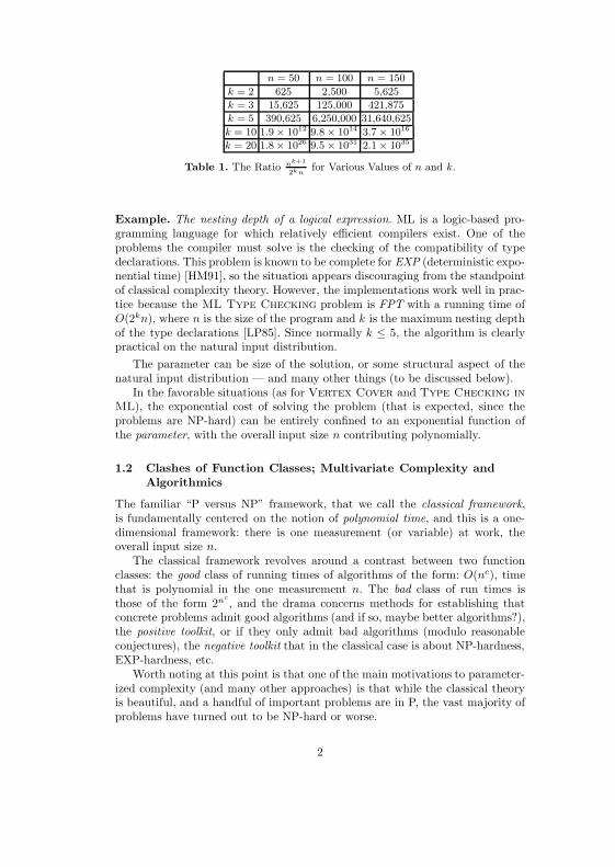
The table below shows the contrast between these two kinds of complexity.In these two example problems, the parameter is the size of the solution being

sought. But a parameter that affects the compexity of a problem can be manythings.

n = 50 n = 100 n = 150

k = 2 625 2,500 5,625

k = 3 15,625 125,000 421,875

k = 5 390,625 6,250,000 31,640,625

k = 10 1.9× 1012 9.8× 1014 3.7× 1016

k = 20 1.8× 1026 9.5× 1031 2.1× 1035

Table 1. The Ratio nk+1

2knfor Various Values of n and k.

Example. The nesting depth of a logical expression. ML is a logic-based pro-gramming language for which relatively efficient compilers exist. One of theproblems the compiler must solve is the checking of the compatibility of typedeclarations. This problem is known to be complete for EXP (deterministic expo-nential time) [HM91], so the situation appears discouraging from the standpointof classical complexity theory. However, the implementations work well in prac-tice because the ML Type Checking problem is FPT with a running time ofO(2kn), where n is the size of the program and k is the maximum nesting depthof the type declarations [LP85]. Since normally k ≤ 5, the algorithm is clearlypractical on the natural input distribution.

The parameter can be size of the solution, or some structural aspect of thenatural input distribution — and many other things (to be discussed below).

In the favorable situations (as for Vertex Cover and Type Checking inML), the exponential cost of solving the problem (that is expected, since theproblems are NP-hard) can be entirely confined to an exponential function ofthe parameter, with the overall input size n contributing polynomially.

1.2 Clashes of Function Classes; Multivariate Complexity andAlgorithmics

The familiar “P versus NP” framework, that we call the classical framework,is fundamentally centered on the notion of polynomial time, and this is a one-dimensional framework: there is one measurement (or variable) at work, theoverall input size n.

The classical framework revolves around a contrast between two functionclasses: the good class of running times of algorithms of the form: O(nc), timethat is polynomial in the one measurement n. The bad class of run times isthose of the form 2nc

, and the drama concerns methods for establishing thatconcrete problems admit good algorithms (and if so, maybe better algorithms?),the positive toolkit, or if they only admit bad algorithms (modulo reasonableconjectures), the negative toolkit that in the classical case is about NP-hardness,EXP-hardness, etc.

Worth noting at this point is that one of the main motivations to parameter-ized complexity (and many other approaches) is that while the classical theoryis beautiful, and a handful of important problems are in P, the vast majority ofproblems have turned out to be NP-hard or worse.

2

Parameterized complexity is basically a two-dimensional sequel, based sim-ilarly on a contrast between two function classes in a two-dimensional setting,where in addition to the overall input size n, we have a second measurement(or variable) that captures something else significant that affects computationalcomplexity (and the opportunities for efficient algorithm design), the parameterk (that might be solution size, or something structural about typical inputs, ...or many other things).

How do we formalize this?

Definition 1. A parameterized language L is a subset L ⊆ Σ∗ × Σ∗. If L is aparameterized language and (x, k) ∈ L then we will refer to x as the main part,and refer to k as the parameter.

A parameter may be non-numerical, and it can also represent an aggregateof various parts or structural properties of the input.

Definition 2. A parameterized language L is multiplicatively fixed-parametertractable if it can be determined in time f(k)q(n) whether (x, k) ∈ L, where|x| = n, q(n) is a polynomial in n, and f is a function (unrestricted).

Definition 3. A parameterized language L is additively fixed-parameter tractableif it can be determined in time f(k) + q(n) whether (x, k) ∈ L, where |x| = n,q(n) is a polynomial in n, and f is a function (unrestricted).

(Easy) Exercise. Show that a parameterized language is additively fixed-parameter tractable if and only if it is multiplicatively fixed-parameter tractable.This emphasizes how cleanly fixed-parameter tractability isolates the computa-tional difficulty in the complexity contribution of the parameter.

The following definition provides us with a place to put all those problemsthat are “solvable in polynomial time for fixed k” without making the centraldistinction about whether this “fixed k” is ending up in the exponent or not (aswith the brute force algorithm for Dominating Set).

Definition 4. A parameterized language L belongs to the class XP if it can bedetermined in time f(k)ng(k) whether (x, k) ∈ L, where |x| = n, with f and gbeing unrestricted functions.

Is it possible that FPT = XP ? This is one of the few structural questionsconcerning parameterized complexity that currently has an answer [DF98].

Theorem 1. FPT is a proper subset of XP.

Summarizing the main point: parameterized complexity is about a naturalbivariate generalization of the P versus NP drama. This inevitably leads to twotoolkits: the positive toolkit of FPT methods (that Daniel Marx will lectureabout), and the negative toolkit that basically provides a parameterized analogof Cook’s Theorem, and methods for showing when fixed-parameter tractablealgorithms for parameterized problems are not possible (modulo reasonable as-sumptions).

There is a larger context captured by the reasonable question that is oftenasked:

3

If Parameterized Complexity is the natural two-dimensional sequel to Pversus NP, then what is the three-dimensional sequel?

Nobody currently knows the answer. Ideally, one would like to have a fullymultivariate perspective on complexity analysis and algorithm design that meetsthe following criteria:• In dimension 1, you get the (basic) P versus NP drama.• In dimension 2, you get the (productive) FPT versus XP drama.• In all dimensions, you have concrete problems where the contrasting outcomesare natural and consequential, and the theory is routinely doable.

Open research problem. Is there such a fully multivariate mathematicalperspective?

Introducing (at least one) secondary variable k beyond the overall input sizen allows us to ask many new and interesting questions that cannot be askedin any mathematically natural way in the classical framework. Much of thisinteresting traction is based on the various ways that parameterization can bedeployed.

1.3 Parameters Can Be Many Things

There are many ways that parameters arise naturally, for example:• The size of a database query. Normally the size of the database is huge, butfrequently queries are small. If n is the size of a relational database, and k is thesize of the query, then answering the query (Model Checking) can be solvedtrivially in time O(nk). It is known that this problem is unlikely to be FPT[DFT96,PY97] because it is hard for W [1], the parameterized analog of NP-hardness. However, if the parameter is the size of the query and the treewidthof the database, then the problem is fixed-parameter tractable [Gr01b].• The number of species in an evolutionary tree. Frequently this parameter isin a range of k ≤ 50. The PHYLIP computational biology server includes analgorithm which solves the Steiner Problem in Hypercubes in order tocompute possible evolutionary trees based on (binary) character information.The exponential heuristic algorithm that is used is in fact an FPT algorithmwhen the parameter is the number of species.• The number of variables or clauses in a logical formula, or the number ofsteps in a deductive procedure. Determining whether at least k clauses of a CNFformula F are satisfiable is FPT with a running time of O(|F |+1.381kk2) [BR99].Since at least half of the m clauses of F can always be satisfied, a more naturalparameterization is to ask if at least m/2 + k clauses can be satisfied — this isFPT with a running time of O(|F |+ 6.92kk2) [BR99]. Implementations indicatethat these algorithms are quite practical [GN00].• The number of moves in a game, or the number of steps in a planning problem.While most game problems are PSPACE-complete classically, it is known thatsome are FPT and others are likely not to be FPT (because they are hardfor W [1]), when parameterized by the number of moves of a winning strategy

4

[ADF95]. The size n of the input game description usually governs the numberof possible moves at any step, so there is a trivial O(nk) algorithm that justexamines the k-step game trees exhaustively.

• The number of facilities to be located. Determining whether a planar graphhas a dominating set of size at most k is fixed-parameter tractable by an algo-rithm with a running time of O(8kn) based on kernelization and search trees.By different methods, an FPT running time of O(336

√k)n can also be proved.

• An unrelated parameter. The input to a problem might come with “extrainformation” because of the way the input arises. For example, we might bepresented with an input graph G together with a k-vertex dominating set in G,and be required to compute an optimal bandwidth layout. Whether this problemis FPT is open.

• The amount of “dirt” in the input or output for a problem. In the MaximumAgreement Subtree (MAST) problem we are presented with a collectionof evolutionary trees trees for a set X of species. These might be obtained bystudying different gene families, for example. Because of errors in the data, thetrees might not be isomorphic, and the problem is to compute the largest possiblesubtree on which they do agree. Parameterized by the number of species thatneed to be deleted to achieve agreement, the MAST problem is FPT by analgorithm having a running time of O(2.27k + rn3) where r is the number oftrees and n is the number of species [NR01].

• The “robustness” of a solution to a problem, or the distance to a solution.For example, given a solution of the Minimum Spanning Tree problem in anedge-weighted graph, we can ask if the cost of the solution is robust under allincreases in the edge costs, where the parameter is the total amount of costincreases.

• The distance to an improved solution. Local search is a mainstay of heuristicalgorithm design. The basic idea is that one maintains a current solution, anditerates the process of moving to a neighboring “better” solution. A neighboringsolution is usually defined as one that is a single step away according to somesmall edit operation between solutions. The following problem is completelygeneral for these situations, and could potentially provide a valuable subroutinefor “speeding up” local search:

k-Speed Up for Local SearchInput: A solution S, k.Parameter: kOutput: The best solution S′ that is within k edit operations of S.

• The goodness of an approximation. If we consider the problem of producingsolutions whose value is within a factor of (1 + ε) of optimal, then we are imme-diately confronted with a natural parameter k = 1/ε. Many of the recent PTASresults for various problems have running times with 1/ε in the exponent of thepolynomial. Since polynomial exponents larger than 3 are not practical, this isa crucial parameter to consider.

5

It is obvious that the practical world is full of concrete problems governedby parameters of all kinds that are bounded in small or moderate ranges. If wecan design algorithms with running times like 2kn for these problems, then wemay have something really useful.

1.4 Kernelization: Another View of FPT

Preprocessing is a practical computing strategy with a lot of power on real worldinput distributions, as shown by the following example.Example: Weihe’s Train Problem

Weihe describes a problem concerning the train systems of Europe [Wei98].Consider a bipartite graph G = (V, E) where V is bipartitioned into two sets S(stations) and T (trains), and where an edge represents that a train t stops ata station s. The relevant graphs are huge, on the order of 10,000 vertices. Theproblem is to compute a minimum number of stations S′ ⊆ S such that everytrain stops at a station in S′. This is a special case of the Hitting Set problem,and is therefore NP-complete.

However, the following two reduction rules can be applied to simplify (pre-process) the input to the problem. In describing these rules, let N (s) denote theset of trains that stop at station s, and let N (t) denote the set of stations atwhich the train t stops.

1. If N (s) ⊆ N (s′) then delete s.2. If N (t) ⊆ N (t′) then delete t′.

Applications of these reduction rules cascade, preserving at each step enoughinformation to obtain an optimal solution. Weihe found that, remarkably, thesetwo simple reduction rules were strong enough to “digest” the original, hugeinput graph into a problem kernel consisting of disjoint components of size atmost 50 — small enough to allow the problem to be solved optimally by bruteforce.

The following is an equivalent definition of FPT [DFS99].

Definition 5. A parameterized language L is kernelizable if there is there is aparameterized transformation of L to itself, and a function g (unrestricted) thatsatisfies:

1. the running time of the transformation of (x, k) into (x′, k′), where |x| = n,is bounded by a polynomial q(n, k) (so that in fact this is a polynomial-time transformation of L to itself, considered classically, although with theadditional structure of a parameterized reduction),

2. k′ ≤ k, and3. |x′| ≤ g(k).

Lemma 1. A parameterized language L is fixed-parameter tractable if and onlyif it is kernelizable.

6

The proof of this is essentially the solution to the second exercise above.The kernelization point of view about FPT has become a major enterprise

all in itself, that will be covered in the lecture by Saket Saurabh.There are several points to be noted about kernelization that lead to impor-

tant research directions:

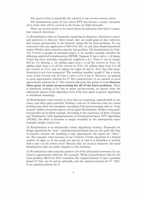
(1) Kernelization rules are frequently surprising in character, laborious to prove,and nontrivial to discover. Once found, they are small gems of data reductionthat remain permanently in the heuristic design file for hard problems. No oneconcerned with any application of Hitting Set on real data should henceforthneglect Weihe’s data reduction rules for this problem. The kernelization for Ver-tex Cover to graphs of minimum degree 4, for another example, includes thefollowing nontrivial transformation [DFS99]. Suppose G has a vertex x of degree3 that has three mutually nonadjacent neighbors a, b, c. Then G can be simpli-fied by: (1) deleting x, (2) adding edges from c to all the vertices in N (a), (3)adding edges from a to all the vertices in N (b), (3) adding edges from b to allthe vertices in N (c), and (4) adding the edges ab and bc. Note that this trans-formation is not even symmetric! The resulting (smaller) graph G′ has a vertexcover of size k if and only if G has a vertex cover of size k. Moreover, an optimalor good approximate solution for G′ lifts constructively to an optimal or goodapproximate solution for G. The research direction this points to is to discoverthese gems of smart preprocessing for all of the hard problems. Thereis absolutely nothing to be lost in smart pre-processing, no matter what thesubsequent phases of the algorithm (even if the next phase is genetic algorithmsor simulated annealing).

(2) Kernelization rules cascade in ways that are surprising, unpredictable in ad-vance, and often quite powerful. Finding a rich set of reduction rules for a hardproblem may allow the synergistic cascading of the pre-processing rules to “wraparound” hidden structural aspects of real input distributions. Weihe’s train prob-lem provides an excellent example. According to the experience of Alber, Grammand Niedermeier with implementations of kernelization-based FPT algorithms[AGN01], the effort to kernelize is amply rewarded by the subsequently expo-nentially smaller search tree.

(3) Kernelization is an intrinsically robust algorithmic strategy. Frequently wedesign algorithms for “pure” combinatorial problems that are not quite like thatin practice, because the modeling is only approximate, the inputs are “dirty”,etc. For example, what becomes of our Vertex Cover algorithm if a limitednumber of edges uv in the graph are special, in that it is forbidden to includeboth u and v in the vertex cover? Because they are local in character, the usualkernelization rules are easily adapted to this situation.

(4) Kernelization rules normally preserve all of the information necessary for op-timal or approximate solutions. For example, Weihe’s kernelization rules for thetrain problem (Hitting Set) transform the original instance G into a problemkernel G′ that can be solved optimally, and the optimal solution for G′ “lifts”to an optimal solution for G.

7

The importance of pre-processing in heuristic design is not a new idea.Cheeseman et al. have previously pointed to its importance in the context ofartificial intelligence algorithms [CKT91]. What parameterized complexity con-tributes is a richer theoretical context for this basic element of practical algo-rithm design. Further research directions include potential methods for mecha-nizing the discovery and/or verification of reduction rules, and data structuresand implementation strategies for efficient kernelization pre-processing.

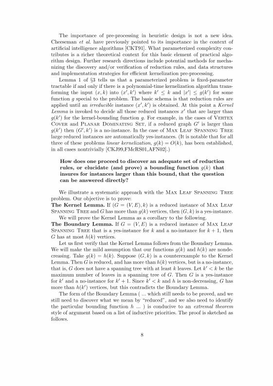
Lemma 1 of §3 tells us that a parameterized problem is fixed-parametertractable if and only if there is a polynomial-time kernelization algorithm trans-forming the input (x, k) into (x′, k′) where k′ ≤ k and |x′| ≤ g(k′) for somefunction g special to the problem. The basic schema is that reduction rules areapplied until an irreducible instance (x′, k′) is obtained. At this point a KernelLemma is invoked to decide all those reduced instances x′ that are larger thang(k′) for the kernel-bounding function g. For example, in the cases of VertexCover and Planar Dominating Set, if a reduced graph G′ is larger thang(k′) then (G′, k′) is a no-instance. In the case of Max Leaf Spanning Treelarge reduced instances are automatically yes-instances. (It is notable that for allthree of these problems linear kernelization, g(k) = O(k), has been established,in all cases nontrivially [CKJ99,FMcRS01,AFN02].)

How does one proceed to discover an adequate set of reductionrules, or elucidate (and prove) a bounding function g(k) thatinsures for instances larger than this bound, that the questioncan be answered directly?

We illustrate a systematic approach with the Max Leaf Spanning Treeproblem. Our objective is to prove:The Kernel Lemma. If (G = (V, E), k) is a reduced instance of Max LeafSpanning Tree and G has more than g(k) vertices, then (G, k) is a yes-instance.

We will prove the Kernel Lemma as a corollary to the following.The Boundary Lemma. If G = (V, E) is a reduced instance of Max LeafSpanning Tree that is a yes-instance for k and a no-instance for k + 1, thenG has at most h(k) vertices.

Let us first verify that the Kernel Lemma follows from the Boundary Lemma.We will make the mild assumption that our functions g(k) and h(k) are nonde-creasing. Take g(k) = h(k). Suppose (G, k) is a counterexample to the KernelLemma. Then G is reduced, and has more than h(k) vertices, but is a no-instance,that is, G does not have a spanning tree with at least k leaves. Let k′ < k be themaximum number of leaves in a spanning tree of G. Then G is a yes-instancefor k′ and a no-instance for k′ + 1. Since k′ < k and h is non-decreasing, G hasmore than h(k′) vertices, but this contradicts the Boundary Lemma.

The form of the Boundary Lemma ( ... which still needs to be proved, and westill need to discover what we mean by “reduced”, and we also need to identifythe particular bounding function h ... ) is conducive to an extremal theoremstyle of argument based on a list of inductive priorities. The proof is sketched asfollows.

8

Sketch Proof of the Boundary Lemma. The proof is by minimum coun-terexample. If there is any counterexample, then we can take G to be one thatsatisfies:(1) G is reduced.(2) G is connected and has more than h(k) vertices.(3) G is a no-instance for k + 1.(4) G is a yes-instance for k, as witnessed by an t-rooted tree subgraph T of Gthat has k leaves. (We do not assume that T is spanning. Note that if T has kleaves then it can be extended to a spanning tree with at least as many leaves.)(5) G is a counterexample where T has a minimum possible number of vertices.(6) Among all of the G, T satisfying (1-5), T has a maximum possible numberof internal vertices that are adjacent to a leaf of T .(7) Among all of the G, T satisfying (1-6), the quantity

∑l∈L d(t, l) is minimized,

where L is the set of leaves of T and d(t, l) is the distance in T to the “root”vertex t.Then we argue for a contradiction.Comment. The point of all this is to set up a framework for argument that willallow us to see what reduction rules are needed, and what g(k) can be achieved.In essence we are setting up a (possibly elaborate, in the spirit of extremal graphtheory) argument by minimum counterexample — and using this as a discoveryprocess for the FPT algorithm design. The witness structure T of condition (4)gives us a way of “coordinatizing” the situation — giving us some structure towork with in our inductive argument. How this strucuture is used will becomeclear as we proceed.

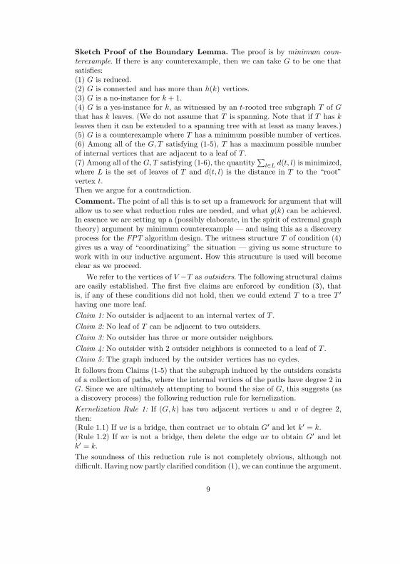
We refer to the vertices of V −T as outsiders. The following structural claimsare easily established. The first five claims are enforced by condition (3), thatis, if any of these conditions did not hold, then we could extend T to a tree T ′

having one more leaf.Claim 1: No outsider is adjacent to an internal vertex of T .Claim 2: No leaf of T can be adjacent to two outsiders.Claim 3: No outsider has three or more outsider neighbors.Claim 4: No outsider with 2 outsider neighbors is connected to a leaf of T .Claim 5: The graph induced by the outsider vertices has no cycles.It follows from Claims (1-5) that the subgraph induced by the outsiders consistsof a collection of paths, where the internal vertices of the paths have degree 2 inG. Since we are ultimately attempting to bound the size of G, this suggests (asa discovery process) the following reduction rule for kernelization.Kernelization Rule 1: If (G, k) has two adjacent vertices u and v of degree 2,then:(Rule 1.1) If uv is a bridge, then contract uv to obtain G′ and let k′ = k.(Rule 1.2) If uv is not a bridge, then delete the edge uv to obtain G′ and letk′ = k.The soundness of this reduction rule is not completely obvious, although notdifficult. Having now partly clarified condition (1), we can continue the argument.

9

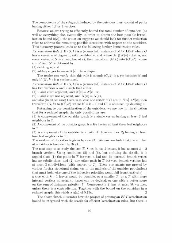
The components of the subgraph induced by the outsiders must consist of pathshaving either 1,2 or 3 vertices.

Because we are trying to efficiently bound the total number of outsiders (aswell as everything else, eventually, in order to obtain the best possible kernel-ization bound h(k)), the situation suggests we should look for further reductionrules to address the remaining possible situations with respect to the outsiders.This discovery process leads us to the following further kernelization rules.Kernelization Rule 2: If (G, k) is a (connected) instance of Max Leaf where Ghas a vertex u of degree 1, with neighbor v, and where ∃x /∈ N (v) (that is, notevery vertex of G is a neighbor of v), then transform (G, k) into (G′, k′), wherek = k′ and G′ is obtained by:(1) deleting u, and(2) adding edges to make N [v] into a clique.

The reader can verify that this rule is sound: (G, k) is a yes-instance if andonly if (G′, k′) is a yes-instance.Kernelization Rule 3: If (G, k) is a (connected) instance of Max Leaf where Ghas two vertices u and v such that either:(1) u and v are adjacent, and N [u] = N [v], or(2) u and v are not adjacent, and N (u) = N (v),and also (in either case) there is at least one vertex of G not in N [u]∪N [v], thentransform (G, k) to (G′, k′) where k′ = k − 1 and G′ is obtained by deleting u.

Returning to our consideration of the outsiders, we are now in the situationthat for a reduced graph, the only possibilities are:(1) A component of the outsider graph is a single vertex having at least 2 leafneighbors in T .(2) A component of the outsider graph is a K2 having at least three leaf neighborsin T .(3) A component of the outsider is a path of three vertices P3 having at leastfour leaf neighbors in T .The weakest of the ratios is given by case (3). We can conclude that the numberof outsiders is bounded by 3k/4.The next step is to study the tree T . Since it has k leaves, it has at most k − 2branch vertices. Using conditions (5) and (6), but omitting the details, it isargued that: (1) the paths in T between a leaf and its parental branch vertexhas no subdivisions, and (2) any other path in T between branch vertices hasat most 3 subdivisions (with respect to T ). These statements are proved byvarious further structural claims (as in the analysis of the outsider population)that must hold, else one of the inductive priorities would fail (constructively) —a tree with k + 1 leaves would be possible, or a smaller T , or a T with moreinternal vertices adjacent to leaves can be devised, or one with a better scoreon the sum-of-distances priority (7). Consequently T has at most 5k vertices,unless there is a contradiction. Together with the bound on the outsiders in areduced graph, this yields a g(k) of 5.75k. ut

The above sketch illustrates how the project of proving an FPT kernelizationbound is integrated with the search for efficient kernelization rules. But there is

10

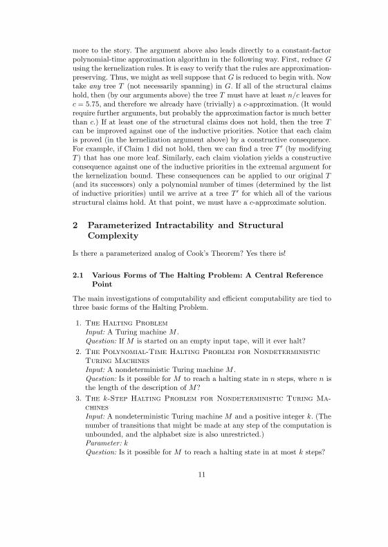
more to the story. The argument above also leads directly to a constant-factorpolynomial-time approximation algorithm in the following way. First, reduce Gusing the kernelization rules. It is easy to verify that the rules are approximation-preserving. Thus, we might as well suppose that G is reduced to begin with. Nowtake any tree T (not necessarily spanning) in G. If all of the structural claimshold, then (by our arguments above) the tree T must have at least n/c leaves forc = 5.75, and therefore we already have (trivially) a c-approximation. (It wouldrequire further arguments, but probably the approximation factor is much betterthan c.) If at least one of the structural claims does not hold, then the tree Tcan be improved against one of the inductive priorities. Notice that each claimis proved (in the kernelization argument above) by a constructive consequence.For example, if Claim 1 did not hold, then we can find a tree T ′ (by modifyingT ) that has one more leaf. Similarly, each claim violation yields a constructiveconsequence against one of the inductive priorities in the extremal argument forthe kernelization bound. These consequences can be applied to our original T(and its successors) only a polynomial number of times (determined by the listof inductive priorities) until we arrive at a tree T ′ for which all of the variousstructural claims hold. At that point, we must have a c-approximate solution.

2 Parameterized Intractability and StructuralComplexity

Is there a parameterized analog of Cook’s Theorem? Yes there is!

2.1 Various Forms of The Halting Problem: A Central ReferencePoint

The main investigations of computability and efficient computability are tied tothree basic forms of the Halting Problem.

1. The Halting ProblemInput: A Turing machine M .Question: If M is started on an empty input tape, will it ever halt?

2. The Polynomial-Time Halting Problem for NondeterministicTuring MachinesInput: A nondeterministic Turing machine M .Question: Is it possible for M to reach a halting state in n steps, where n isthe length of the description of M?

3. The k-Step Halting Problem for Nondeterministic Turing Ma-chinesInput: A nondeterministic Turing machine M and a positive integer k. (Thenumber of transitions that might be made at any step of the computation isunbounded, and the alphabet size is also unrestricted.)Parameter: kQuestion: Is it possible for M to reach a halting state in at most k steps?

11

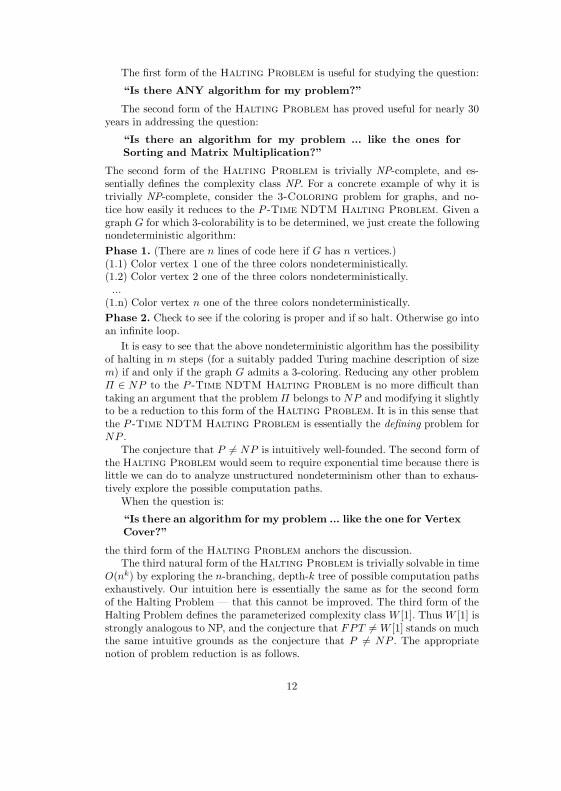
The first form of the Halting Problem is useful for studying the question:

“Is there ANY algorithm for my problem?”

The second form of the Halting Problem has proved useful for nearly 30years in addressing the question:

“Is there an algorithm for my problem ... like the ones forSorting and Matrix Multiplication?”

The second form of the Halting Problem is trivially NP-complete, and es-sentially defines the complexity class NP. For a concrete example of why it istrivially NP-complete, consider the 3-Coloring problem for graphs, and no-tice how easily it reduces to the P -Time NDTM Halting Problem. Given agraph G for which 3-colorability is to be determined, we just create the followingnondeterministic algorithm:Phase 1. (There are n lines of code here if G has n vertices.)(1.1) Color vertex 1 one of the three colors nondeterministically.(1.2) Color vertex 2 one of the three colors nondeterministically....

(1.n) Color vertex n one of the three colors nondeterministically.Phase 2. Check to see if the coloring is proper and if so halt. Otherwise go intoan infinite loop.

It is easy to see that the above nondeterministic algorithm has the possibilityof halting in m steps (for a suitably padded Turing machine description of sizem) if and only if the graph G admits a 3-coloring. Reducing any other problemΠ ∈ NP to the P -Time NDTM Halting Problem is no more difficult thantaking an argument that the problem Π belongs to NP and modifying it slightlyto be a reduction to this form of the Halting Problem. It is in this sense thatthe P -Time NDTM Halting Problem is essentially the defining problem forNP .

The conjecture that P 6= NP is intuitively well-founded. The second form ofthe Halting Problem would seem to require exponential time because there islittle we can do to analyze unstructured nondeterminism other than to exhaus-tively explore the possible computation paths.

When the question is:

“Is there an algorithm for my problem ... like the one for VertexCover?”

the third form of the Halting Problem anchors the discussion.The third natural form of the Halting Problem is trivially solvable in time

O(nk) by exploring the n-branching, depth-k tree of possible computation pathsexhaustively. Our intuition here is essentially the same as for the second formof the Halting Problem — that this cannot be improved. The third form of theHalting Problem defines the parameterized complexity class W [1]. Thus W [1] isstrongly analogous to NP, and the conjecture that FPT 6= W [1] stands on muchthe same intuitive grounds as the conjecture that P 6= NP . The appropriatenotion of problem reduction is as follows.

12

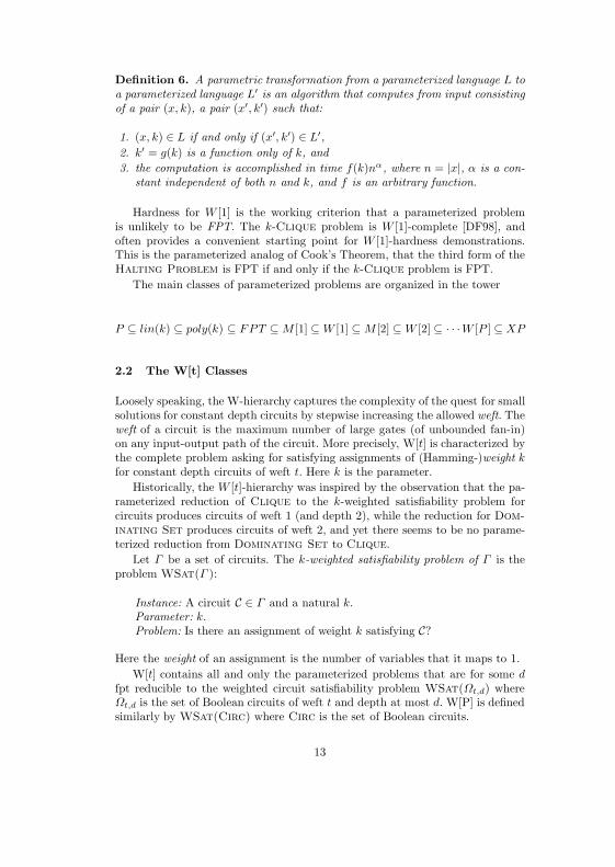
Definition 6. A parametric transformation from a parameterized language L toa parameterized language L′ is an algorithm that computes from input consistingof a pair (x, k), a pair (x′, k′) such that:

1. (x, k) ∈ L if and only if (x′, k′) ∈ L′,2. k′ = g(k) is a function only of k, and3. the computation is accomplished in time f(k)nα, where n = |x|, α is a con-

stant independent of both n and k, and f is an arbitrary function.

Hardness for W [1] is the working criterion that a parameterized problemis unlikely to be FPT. The k-Clique problem is W [1]-complete [DF98], andoften provides a convenient starting point for W [1]-hardness demonstrations.This is the parameterized analog of Cook’s Theorem, that the third form of theHalting Problem is FPT if and only if the k-Clique problem is FPT.

The main classes of parameterized problems are organized in the tower

P ⊆ lin(k) ⊆ poly(k) ⊆ FPT ⊆ M [1] ⊆ W [1] ⊆ M [2] ⊆ W [2] ⊆ · · ·W [P ] ⊆ XP

2.2 The W[t] Classes

Loosely speaking, the W-hierarchy captures the complexity of the quest for smallsolutions for constant depth circuits by stepwise increasing the allowed weft. Theweft of a circuit is the maximum number of large gates (of unbounded fan-in)on any input-output path of the circuit. More precisely, W[t] is characterized bythe complete problem asking for satisfying assignments of (Hamming-)weight kfor constant depth circuits of weft t. Here k is the parameter.

Historically, the W [t]-hierarchy was inspired by the observation that the pa-rameterized reduction of Clique to the k-weighted satisfiability problem forcircuits produces circuits of weft 1 (and depth 2), while the reduction for Dom-inating Set produces circuits of weft 2, and yet there seems to be no parame-terized reduction from Dominating Set to Clique.

Let Γ be a set of circuits. The k-weighted satisfiability problem of Γ is theproblem WSat(Γ ):

Instance: A circuit C ∈ Γ and a natural k.Parameter: k.Problem: Is there an assignment of weight k satisfying C?

Here the weight of an assignment is the number of variables that it maps to 1.W[t] contains all and only the parameterized problems that are for some d

fpt reducible to the weighted circuit satisfiability problem WSat(Ωt,d) whereΩt,d is the set of Boolean circuits of weft t and depth at most d. W[P] is definedsimilarly by WSat(Circ) where Circ is the set of Boolean circuits.

13

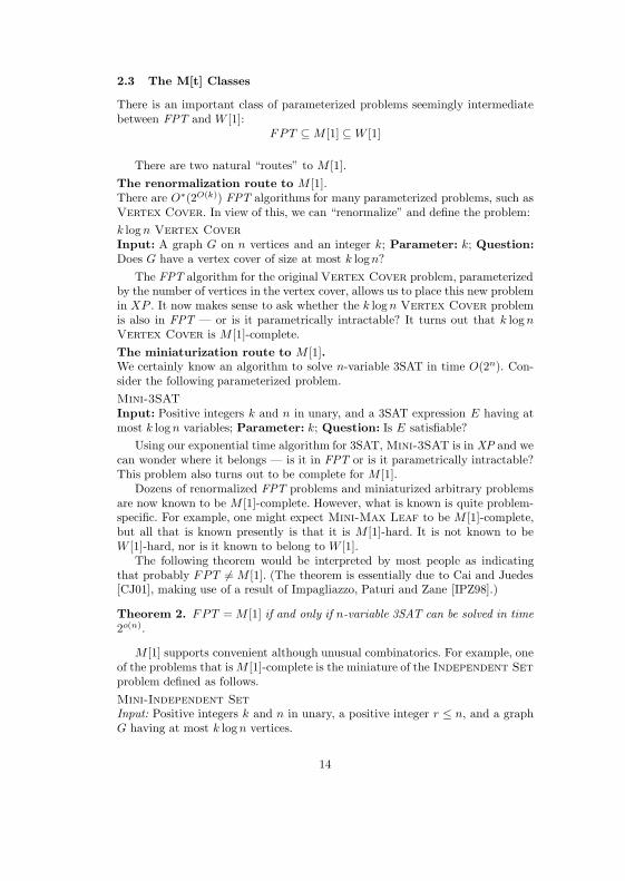
2.3 The M[t] Classes

There is an important class of parameterized problems seemingly intermediatebetween FPT and W [1]:

FPT ⊆ M [1] ⊆ W [1]

There are two natural “routes” to M [1].The renormalization route to M [1].There are O∗(2O(k)) FPT algorithms for many parameterized problems, such asVertex Cover. In view of this, we can “renormalize” and define the problem:k log n Vertex CoverInput: A graph G on n vertices and an integer k; Parameter: k; Question:Does G have a vertex cover of size at most k logn?

The FPT algorithm for the original Vertex Cover problem, parameterizedby the number of vertices in the vertex cover, allows us to place this new problemin XP . It now makes sense to ask whether the k log n Vertex Cover problemis also in FPT — or is it parametrically intractable? It turns out that k log nVertex Cover is M [1]-complete.The miniaturization route to M [1].We certainly know an algorithm to solve n-variable 3SAT in time O(2n). Con-sider the following parameterized problem.Mini-3SATInput: Positive integers k and n in unary, and a 3SAT expression E having atmost k log n variables; Parameter: k; Question: Is E satisfiable?

Using our exponential time algorithm for 3SAT, Mini-3SAT is in XP and wecan wonder where it belongs — is it in FPT or is it parametrically intractable?This problem also turns out to be complete for M [1].

Dozens of renormalized FPT problems and miniaturized arbitrary problemsare now known to be M [1]-complete. However, what is known is quite problem-specific. For example, one might expect Mini-Max Leaf to be M [1]-complete,but all that is known presently is that it is M [1]-hard. It is not known to beW [1]-hard, nor is it known to belong to W [1].

The following theorem would be interpreted by most people as indicatingthat probably FPT 6= M [1]. (The theorem is essentially due to Cai and Juedes[CJ01], making use of a result of Impagliazzo, Paturi and Zane [IPZ98].)

Theorem 2. FPT = M [1] if and only if n-variable 3SAT can be solved in time2o(n).

M [1] supports convenient although unusual combinatorics. For example, oneof the problems that is M [1]-complete is the miniature of the Independent Setproblem defined as follows.Mini-Independent SetInput: Positive integers k and n in unary, a positive integer r ≤ n, and a graphG having at most k log n vertices.

14

Parameter: kQuestion: Does G have an independent set of size at least r?

Theorem 3. There is an FPT reduction from Mini-Independent Set to ordi-nary parameterized Independent Set (parameterized by the number of verticesin the independent set).

Proof. Let G = (V, E) be the miniature, for which we wish to determine whetherG has an independent set of size r. Here, of course, |V | ≤ k logn and we mayregard the vertices of G as organized in k blocks V1, ..., Vk of size log n. Wenow employ a simple but useful counting trick that can be used when reducingminiatures to “normal” parameterized problems. Our reduction is a Turing re-duction, with one branch for each possible way of writing r as a sum of k terms,r = r1 + · · · + rk, where each ri is bounded by logn. The reader can verifythat (log n)k is an FPT function, and thus that there are an allowed number ofbranches. A branch represents a commitment to choose ri vertices from block Vi

(for each i) to be in the independent set.We now produce (for a given branch of the Turing reduction) a graph G′

that has an independent set of size k if and only if the miniature G has anindependent set of size r, distributed as indicated by the commitment madeon that branch. The graph G′ consists of k cliques, together with some edgesbetween these cliques. The ith clique consists of vertices in 1:1 correspondencewith the subsets of Vi of size ri. An edge connects a vertex x in the ith cliqueand a vertex y in the jth clique if and only if there is a vertex u in the subsetSx ⊆ Vi represented by x, and a vertex v in the subset Sy ⊆ Vj represented byy, such that uv ∈ E. Verification is straightforward.

The theorem above shows that M [1] is contained in W [1].Cai and Juedes [CJ01] proved the following, opening up a broad program of

studying the optimality of FPT algorithms.

Theorem 4. If FPT 6= M [1] then there cannot be an FPT algorithm for thegeneral Vertex Cover problem with a parameter function of the form f(k) =2o(k), and there cannot be an FPT algorithm for the Planar Vertex Cover

problem with a parameter function of the form f(k) = 2o(√

k).

It has previously been known that Planar Dominating Set, parameter-ized by the number n of vertices in the graph can be solved optimally in timeO∗(2O(

√n)) by using the Lipton-Tarjan Planar Separator Theorem. Combining

the lower bound theorem of Cai-Juedes with the linear kernelization result ofAlber et al. [AFN02] shows that this cannot be improved to O∗(2o(

√n)) unless

FPT = M [1].

2.4 An Example of a W [1]-hardness Reduction

We take as our example, how parameterized complexity can be used to studythe complexity of approximation. Approximation immediately concerns a fun-damental parameter: k = 1/ε, the goodness of the approximation.

15

To illustrate the issue, consider the following more-or-less random sample ofrecent PTAS results:

– The PTAS for the Euclidean TSP due to Arora [Ar96] has a running timeof around O(n3000/ε). Thus for a 20% error, we have a “polynomial-time”algorithm that runs in time O(n15000).

– The PTAS for the Multiple Knapsack problem due to Chekuri and Khanna[CK00] has a running time of O(n12(log(1/ε)/ε8)). Thus for a 20% error we havea polynomial-time algorithm that runs in time O(n9375000).

– The PTAS for the Minimum Cost Routing Spanning Tree problem dueto Wu, Lancia, Banfna, Chao, Ravi and Tang [WLBCRT98] has a runningtime of O(n2d2/εe−2). For a 20% error, we thus have a running time of O(n18).

– The PTAS for the Unbounded Batch Scheduling problem due to Deng,Feng, Zhang and Zhu [DFZZ01] has a running time of O(n5 log1+ε(1+(1/ε))).Thus for a 20% error we have an O(n50) polynomial-time algorithm.

– The PTAS for Two-Vehicle Scheduling on a Path due to Karuno andNagamochi [KN01] has a running time of O(n8(1+(2/ε))); thus O(n88) for a20% error.

– The PTAS for the Maximum Subforest Problem due to Shamir andTsur [ST98] has a running time of O(n221/ε−1). For a 20% error we thushave a “polynomial” running time of O(n958267391).

– The PTAS for the Maximum Indendent Set problem on geometric graphsdue to Erlebach, Jansen and Seidel [EJS01] has a running time ofO(n(4/π)(1/ε2+2)2(1/ε2+1)2). Thus for a 20% error we have a running time ofO(n532804).

– The PTAS for the Class-Constrained Packing Problem due to Shachnaiand Tamir [ST00] has a running time (for 3 colors) of O(n64/ε+(log(1/ε)/ε8)).Thus for a 20% error (for 3 colors) we have a running time of O(n1021570).

– The PTAS for the problem of Base Station Positioning in UMTS Net-works due to Galota, Glasser, Reith and Vollmer [GGRV01] has a runningtime of O(n25/ε2), and thus O(n627) time for a 20% error.

– The PTAS for the General Multiprocessor Job Scheduling Problemdue to Chen and Miranda [CM99] runs in time O(n(3mm!)(m/ε)+1

) for m ma-chines. Thus for 4 machines with a 20% error we have an algorithm that runsin time O(n100000000000000000000000000000000000000000000000000000000000000000000)or so.

Since polynomial-time algorithms with exponent greater than 3 are generallynot very practical, the following question would seem to be important.

Can we get the k = 1/ε out of the exponent?

The following definition captures the essential issue.

Definition 7. An optimization problem Π has an efficient P -time approxima-tion scheme (EPTAS) if it can be approximated to a goodness of (1+ε) of optimalin time f(k)nc where c is a constant and k = 1/ε.

16

In 1997, Arora gave an EPTAS for the Euclidean TSP [Ar97].The following easy but important connection between parameterized com-

plexity and approximation was first proved by Bazgan [Baz95,CT97].

Theorem 5. Suppose that Πopt is an optimization problem, and that Πparam

is the corresponding parameterized problem, where the parameter is the value ofan optimal solution. Then Πparam is fixed-parameter tractable if Πopt has anefficient PTAS.

Applying Bazgan’s Theorem is not necessarily difficult — we will sketch herea recent example. Khanna and Motwani introduced three planar logic problemsin an interesting effort to give a general explanation of PTAS-approximability.Their suggestion is that “hidden planar structure” in the logic of an optimizationproblem is what allows PTASs to be developed [KM96]. They gave examples ofoptimization problems known to have PTASs, problems having nothing to dowith graphs, that could nevertheless be reduced to these planar logic problems.The PTASs for the planar logic problems thus “explain” the PTASs for theseother problems. Here is one of their three general planar logic optimization prob-lems.Planar TMINInput: A collection of Boolean formulas in sum-of-products form, with all literalspositive, where the associated bipartite graph is planar (this graph has a vertexfor each formula and a vertex for each variable, and an edge between two suchvertices if the variable occurs in the formula).Output: A truth assignment of minimum weight (i.e., a minimum number ofvariables set to true) that satisfies all the formulas.

The following theorem is from joint work with Cai, Juedes and Rosamond[CFJR01].

Theorem 6. Planar TMIN is hard for W [1] and therefore does not have anEPTAS unless FPT = W [1].

Proof. We show that Clique is parameterized reducible to Planar TMINwith the parameter being the weight of a truth assignment. Since Clique isW[1]-complete, it will follow that the parameterized form of Planar TMIN isW[1]-hard.

To begin, let 〈G, k〉 be an instance of Clique. Assume that G has n vertices.From G and k, we will construct a collection C of FOFs (sum-of-products for-mulas) over f(k) blocks of n variables. C will contain at most 2f(k) FOFs andthe incidence graph of C will be planar. Moreover, each minterm in each FOFwill contain at most 4 variables. The collection C is constructed so that G hasa clique of size k if and only if C has a weight f(k) satisfying assignment withexactly one variable set to true in each block of n variables. Here we have thatf(k) = O(k4).

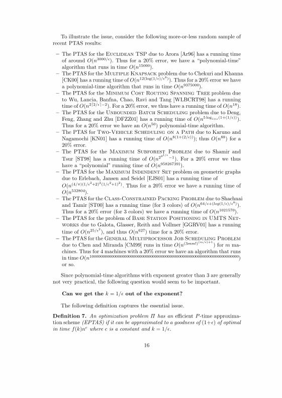
To maintain planarity in the incidence graph for C, we ensure that each blockof n variables appears in at most 2 FOFs. If this condition is maintained, thenwe can draw each block of n variables as follows.

17

v3

v2

v1

vn

FOFFOF

We describe the construction in two stages. In the first stage, we use k blocksof n variables and a collection C′ of k(k−1)/2+k FOFs. In a weight k satisfyingassignment for C′, exactly one variable vi, j in each block of variables bi =[vi,1, . . . , vi,n] will be set to true. We interpret this event as “vertex j is the ithvertex in the clique of size k.” The k(k−1)/2+k FOFs are described as follows.

For each 1 ≤ i ≤ k, let fi be the FOFn∨

j=1

vi,j. This FOF ensures that at least

one variable in bi is set to true. For each pair 1 ≤ i < j ≤ k, let fi,j be the FOF∨(u,v)∈E

vi,uvj,v. Each FOF fi,j ensures that there is an edge in G between the

ith vertex the clique and the jth vertex in the clique.

It is somewhat straightforward to show that C′ = f1, . . . , fk, f1,2, . . . , fk−1,khas a weight k satisfying assignment if and only if G has a clique of size k. To seethis, notice that any weight k satisfying assignment for C′ must satisfy exactly1 variable in each block bi. Each first order formula fi,j ensures that there isan edge between the ith vertex in the potential clique and the jth vertex in thepotential clique. Notice also that, since we assume that G does not contain edgesof the form (u, u), the FOF fi,j also ensures that the ith vertex in the potentialclique is not the jth vertex in the potential clique. This completes the first stage.

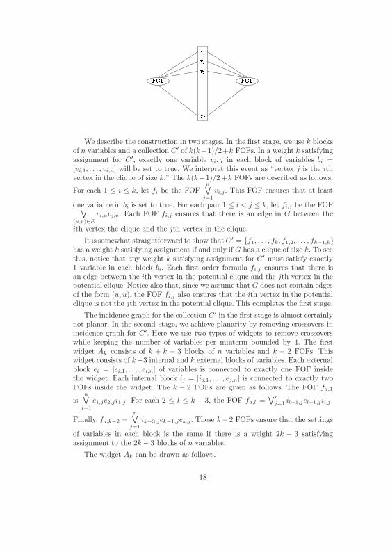
The incidence graph for the collection C′ in the first stage is almost certainlynot planar. In the second stage, we achieve planarity by removing crossovers inincidence graph for C′. Here we use two types of widgets to remove crossoverswhile keeping the number of variables per minterm bounded by 4. The firstwidget Ak consists of k + k − 3 blocks of n variables and k − 2 FOFs. Thiswidget consists of k−3 internal and k external blocks of variables. Each externalblock ei = [ei,1, . . . , ei,n] of variables is connected to exactly one FOF insidethe widget. Each internal block ij = [ij,1, . . . , ej,n] is connected to exactly twoFOFs inside the widget. The k − 2 FOFs are given as follows. The FOF fa,1

isn∨

j=1

e1,je2,ji1,j. For each 2 ≤ l ≤ k − 3, the FOF fa,l =∨n

j=1 il−1,jel+1,j il,j .

Finally, fa,k−2 =n∨

j=1ik−3,jek−1,jek,j. These k− 2 FOFs ensure that the settings

of variables in each block is the same if there is a weight 2k − 3 satisfyingassignment to the 2k− 3 blocks of n variables.

The widget Ak can be drawn as follows.

18

fa;k3.........

.........

fa;1 fa;2 fa;k2

............

e1 e2 e3 ek1 ek

ik3i2i1

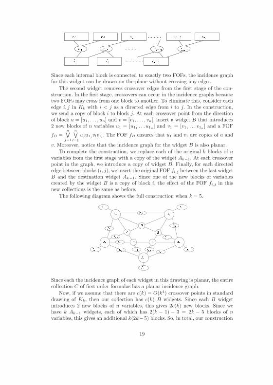
Since each internal block is connected to exactly two FOFs, the incidence graphfor this widget can be drawn on the plane without crossing any edges.

The second widget removes crossover edges from the first stage of the con-struction. In the first stage, crossovers can occur in the incidence graphs becausetwo FOFs may cross from one block to another. To eliminate this, consider eachedge i, j in Kk with i < j as a directed edge from i to j. In the construction,we send a copy of block i to block j. At each crossover point from the directionof block u = [u1, . . . , un] and v = [v1, . . . , vn], insert a widget B that introduces2 new blocks of n variables u1 = [u11 . . .u1n ] and v1 = [v11 . . . v1n ] and a FOF

fB =n∨

j=1

n∨l=1

uju1jvlv1l . The FOF fB ensures that u1 and v1 are copies of u and

v. Moreover, notice that the incidence graph for the widget B is also planar.To complete the construction, we replace each of the original k blocks of n

variables from the first stage with a copy of the widget Ak−1. At each crossoverpoint in the graph, we introduce a copy of widget B. Finally, for each directededge between blocks (i, j), we insert the original FOF fi,j between the last widgetB and the destination widget Ak−1. Since one of the new blocks of variablescreated by the widget B is a copy of block i, the effect of the FOF fi,j in thisnew collections is the same as before.

The following diagram shows the full construction when k = 5.

f1;2

f1;4 f2;4

f3;4

f2;3

f1;5

f2;5

f3;5

f4;5

B

B

B

BB

A5

A5 A5

A5A5

f1;3

f1 f2

f3

f4

f5

Since each the incidence graph of each widget in this drawing is planar, the entirecollection C of first order formulas has a planar incidence graph.

Now, if we assume that there are c(k) = O(k4) crossover points in standarddrawing of Kk, then our collection has c(k) B widgets. Since each B widgetintroduces 2 new blocks of n variables, this gives 2c(k) new blocks. Since wehave k Ak−1 widgets, each of which has 2(k − 1) − 3 = 2k − 5 blocks of nvariables, this gives an additional k(2k−5) blocks. So, in total, our construction

19

has f(k) = 2c(k) + 2k2 − 5k = O(k4) blocks of n variables. Note also that thereare g(k) = k(k − 1)/2 + k(k − 2) + c(k) = O(k4) FOFs in the collection C.

As shown in our construction C has a weight f(k) satisfying assignment (i.e.,each block has exactly one variable set to true) if and only if the original graph Ghas a clique of size k. Since the incidence graph of C is planar and each mintermin each FOF contains at most four variables, it follows that this construction isa parameterized reduction as claimed. ut

In a similar manner the other two planar logic problems defined by Khannaand Motwani can also be shown to be W [1]-hard.

3 Recommended Books and Articles

Parameterized Complexity – R. Downey and M. Fellows, Springer, 1999.Parameterized Complexity Theory – J. Flum and M. Grohe, Springer, 2006.Invitation to Fixed Parameter Algorithms – R. Niedermeier, Oxford Univ. Press,2006.The Computer Journal, 2008, Numbers 1 and 3 – a double special issue of surveysof various aspects and application areas of parameterized complexity.

References

[ADF95] K. Abrahamson, R. Downey and M. Fellows, “Fixed Parameter Tractabilityand Completeness IV: On Completeness for W [P ] and PSPACE Analogs,” Annalsof Pure and Applied Logic 73 (1995), 235–276.

[AFN01] J. Alber, H. Fernau and R. Niedermeier, “Parameterized Complexity: Expo-nential Speed-Up for Planar Graph Problems,” in: Proceedings of ICALP 2001,Crete, Greece, Lecture Notes in Computer Science vol. 2076 (2001), 261-272.

[AFN02] J. Alber, M. Fellows and R. Niedermeier, “Efficient Data Reduction for Dom-inating Set: A Linear Problem Kernel for the Planar Case,” to appear in theProceedings of Scandinavian Workshop on Algorithms and Theory (SWAT 2002),Springer-Verlag, Lecture Notes in Computer Science, 2002.

[AGN01] J. Alber, J. Gramm and R. Niedermeier, “Faster Exact Algorithms for HardProblems: A Parameterized Point of View,” Discrete Mathematics 229 (2001), 3–27.

[Ar96] S. Arora, “Polynomial Time Approximation Schemes for Euclidean TSP andOther Geometric Problems,” In: Proceedings of the 37th IEEE Symposium on Foun-dations of Computer Science, 1996, pp. 2–12.

[Ar97] S. Arora, “Nearly Linear Time Approximation Schemes for Euclidean TSP andOther Geometric Problems,” Proc. 38th Annual IEEE Symposium on the Founda-tions of Computing (FOCS’97), IEEE Press (1997), 554-563.

[Baz95] C. Bazgan, “Schemas d’approximation et complexite parametree,” Rapportde stage de DEA d’Informatique a Orsay, 1995.

[BR99] N. Bansal and V. Raman, “Upper Bounds for MaxSat: Further Improved,”Proc. 10th International Symposium on Algorithms and Computation (ISAAC ’99),Springer-Verlag, Lecture Notes in Computer Science 1741 (1999), 247–258.

20

[CFJR01] Liming Cai, M. Fellows, D. Juedes and F. Rosamond, “Efficient Polynomial-Time Approximation Schemes for Problems on Planar Structures: Upper andLower Bounds,” manuscript, 2001.

[CJ01] L. Cai and D. Juedes. “On the Existence of Subexponential ParameterizedAlgorithms,” manuscript, 2001. Revised version of the paper, “Subexponential Pa-rameterized Algorithms Collapse the W-Hierarchy,” in: Proceedings 28th ICALP,Springer-Verlag LNCS 2076 (2001), 273–284.

[CK00] C. Chekuri and S. Khanna, “A PTAS for the Multiple Knapsack Problem,”Proceedings of the ACM-SIAM Symposium on Discrete Algorithms (SODA 2000),pp. 213-222.

[CKJ99] J. Chen, I.A. Kanj and W. Jia, “Vertex Cover: Further Observations andFurther Improvements,” Proceedings of the 25th International Workshop on Graph-Theoretic Concepts in Computer Science (WG’99), Lecture Notes in ComputerScience 1665 (1999), 313–324.

[CKT91] P. Cheeseman, B. Kanefsky and W. Taylor, “Where the Really Hard Prob-lems Are,” Proc. 12th International Joint Conference on Artificial Intelligence(1991), 331-337.

[CM99] J. Chen and A. Miranda, “A Polynomial-Time Approximation Scheme forGeneral Multiprocessor Scheduling,” Proc. ACM Symposium on Theory of Com-puting (STOC ’99), ACM Press (1999), 418–427.

[CS97] Leizhen Cai and B. Schieber, “A Linear Time Algorithm for Computing theIntersection of All Odd Cycles in a Graph,” Discrete Applied Math. 73 (1997),27-34.

[CT97] M. Cesati and L. Trevisan, “On the Efficiency of Polynomial Time Approxi-mation Schemes,” Information Processing Letters 64 (1997), 165–171.

[CW95] M. Cesati and H. T. Wareham, “Parameterized Complexity Analysis in RobotMotion Planning,” Proceedings 25th IEEE Intl. Conf. on Systems, Man and Cy-bernetics: Volume 1, IEEE Press, Los Alamitos, CA (1995), 880-885.

[DF98] R. G. Downey and M. R. Fellows, Parameterized Complexity, Springer-Verlag,1998.

[DFS99] R. G. Downey, M. R. Fellows and U. Stege, “Parameterized Complexity: AFramework for Systematically Confronting Computational Intractability.” In: Con-temporary Trends in Discrete Mathematics, (R. Graham, J. Kratochvıl, J. Nesetriland F. Roberts, eds.), Proceedings of the DIMACS-DIMATIA Workshop, Prague,1997, AMS-DIMACS Series in Discrete Mathematics and Theoretical ComputerScience, vol. 49 (1999), 49–99.

[DFT96] R. G. Downey, M. Fellows and U. Taylor, “The Parameterized Complexityof Relational Database Queries and an Improved Characterization of W [1],” in:Combinatorics, Complexity and Logic: Proceedings of DMTCS’96, Springer-Verlag(1997), 194–213.

[DFZZ01] X. Deng, H. Feng, P. Zhang and H. Zhu, “A Polynomial Time Approxima-tion Scheme for Minimizing Total Completion Time of Unbounded Batch Schedul-ing,” Proc. 12th International Symposium on Algorithms and Computation (ISAAC’01), Springer-Verlag, Lecture Notes in Computer Science 2223 (2001), 26–35.

[EJS01] T. Erlebach, K. Jansen and E. Seidel, “Polynomial Time ApproximationSchemes for Geometric Graphs,” Proc. ACM Symposium on Discrete Algorithms(SODA’01), 2001, pp. 671–679.

[FG01] J. Flum and M. Grohe, “Describing Parameterized Complexity Classes,”manuscript, 2001.

21

[FMcRS01] M. Fellows, C. McCartin, F. Rosamond and U. Stege, “Trees with Few andMany Leaves,” manuscript, full version of the paper: “Coordinatized kernels andcatalytic reductions: An improved FPT algorithm for max leaf spanning tree andother problems,” Proceedings of the 20th FST TCS Conference, New Delhi, India,Lecture Notes in Computer Science vol. 1974, Springer Verlag (2000), 240-251.

[GGRV01] M. Galota, C. Glasser, S. Reith and H. Vollmer, “A Polynomial Time Ap-proximation Scheme for Base Station Positioning in UMTS Networks,” Proc. Dis-crete Algorithms and Methods for Mobile Computing and Communication, 2001.

[GN00] J. Gramm and R. Niedermeier, “Faster Exact Algorithms for Max2Sat,” Proc.4th Italian Conference on Algorithms and Complexity, Springer-Verlag, LectureNotes in Computer Science 1767 (2000), 174–186.

[Gr01a] M. Grohe, “Generalized Model-Checking Problems for First-Order Logic,”Proc. STACS 2001, Springer-Verlag LNCS vol. 2001 (2001), 12–26.

[Gr01b] M. Grohe, “The Parameterized Complexity of Database Queries,” Proc. PODS2001, ACM Press (2001), 82–92.

[GSS01] G. Gottlob, F. Scarcello and M. Sideri, “Fixed Parameter Complexity in AIand Nonmonotonic Reasoning,” to appear in The Artificial Intelligence Journal.Conference version in: Proc. of the 5th International Conference on Logic Pro-gramming and Nonmonotonic Reasoning (LPNMR’99), vol. 1730 of Lecture Notesin Artificial Intelligence (1999), 1–18.

[HM91] F. Henglein and H. G. Mairson, “The Complexity of Type Inference for Higher-Order Typed Lambda Calculi.” In Proc. Symp. on Principles of ProgrammingLanguages (POPL) (1991), 119-130.

[IPZ98] R. Impagliazzo, R. Paturi and F. Zane. “Which Problems Have Strongly Expo-nential Complexity?” Proceedings of the 39th Annual Symposium on Foundationsof Computer Science (FOCS’1998), 653–663.

[KM96] S. Khanna and R. Motwani, “Towards a Syntactic Characterization of PTAS,”in: Proc. STOC 1996, ACM Press (1996), 329–337.

[KN01] Y. Karuno and H. Nagamochi, “A Polynomial Time Approximation Schemefor the Multi-vehicle Scheduling Problem on a Path with Release and HandlingTimes,” Proc. 12th International Symposium on Algorithms and Computation(ISAAC ’01), Springer-Verlag, Lecture Notes in Computer Science 2223 (2001),36–47.

[KR00] S. Khot and V. Raman, ‘Parameterized Complexity of Finding Subgraphs withHereditary properties’, Proceedings of the Sixth Annual International Computingand Combinatorics Conference (COCOON 2000) July 2000, Sydney, Australia,Lecture Notes in Computer Science, Springer Verlag 1858 (2000) 137-147.

[LP85] O. Lichtenstein and A. Pneuli. “Checking That Finite-State Concurrents Pro-grams Satisfy Their Linear Specification.” In: Proceedings of the 12th ACM Sym-posium on Principles of Programming Languages (1985), 97–107.

[MR99] M. Mahajan and V. Raman, “Parameterizing Above Guaranteed Values:MaxSat and MaxCut,” J. Algorithms 31 (1999), 335-354.

[NR01] R. Niedermeier and P. Rossmanith, “An Efficient Fixed Parameter Algorithmfor 3-Hitting Set,” Journal of Discrete Algorithms 2(1), 2001.

[NSS98] A. Natanzon, R. Shamir and R. Sharan, “A Polynomial-Time Approxima-tion Algorithm for Minimum Fill-In,” Proc. ACM Symposium on the Theory ofComputing (STOC’98), ACM Press (1998), 41–47.

[PY97] C. Papadimitriou and M. Yannakakis, “On the Complexity of DatabaseQueries,” Proc. ACM Symp. on Principles of Database Systems (1997), 12–19.

22

[ST98] R. Shamir and D. Tzur, “The Maximum Subforest Problem: Approxima-tion and Exact Algorithms,” Proc. ACM Symposium on Discrete Algorithms(SODA’98), ACM Press (1998), 394–399.

[ST00] H. Shachnai and T. Tamir, “Polynomial Time Approximation Schemes forClass-Constrained Packing Problems,” Proc. APPROX 2000.

[St00] U. Stege, “Resolving Conflicts in Problems in Computational Biochemistry,”Ph.D. dissertation, ETH, 2000.

[Wei98] K. Weihe, “Covering Trains by Stations, or the Power of Data Reduction,”Proc. ALEX’98 (1998), 1–8.

[Wei00] K. Weihe, “On the Differences Between ‘Practical’ and ‘Applied’ (invited pa-per),” Proc. WAE 2000, Springer-Verlag, Lecture Notes in Computer Science 1982(2001), 1–10.

[WLBCRT98] B. Wu, G. Lancia, V. Bafna, K-M. Chao, R. Ravi and C. Tang, “APolynomial Time Approximation Scheme for Minimum Routing Cost SpanningTrees,” Proc. SODA ’98, 1998, pp. 21–32.

23

Fedor Fomin

Gridology

Gridology

Fed

orV

.Fom

in

Dep

artmen

tofIn

formatics,

University

ofB

ergen

,N

orway

AG

APE

2009

Exam

ple:T

hecity

ofBergen

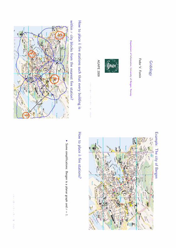
How

toplace

kfire

stationssuch

thatevery

buildingis

within

rcity

blocks

fromthe

nearestfire

station?

How

toplace

kfire

stations?

Som

esim

plifi

cations:

Bergen

isa

plan

argrap

han

dr=1.

How

toplace

kfire

stations?

Som

esim

plifi

cations:

Bergen

isa

plan

argrap

han

dr=1.

T

here

isa

linear

kernel

O(k)

fordom

inatin

gset

onplan

ar

graph,so2

O(k

)nO

(1)

algorithm

ispossib

le

How

toplace

kfire

stations?

Som

esim

plifi

cations:

Bergen

isa

plan

argrap

han

dr=1.

T

here

isa

linear

kernel

O(k)

fordom

inatin

gset

onplan

ar

graph,so2

O(k

)nO

(1)

algorithm

ispossib

le

W

esh

owhow

toget

subexp

onen

tial2 √kn

O(1

)algorith

ms.

How

toplace

kfire

stations?

Som

esim

plifi

cations:

Bergen

isa

plan

argrap

han

dr=1.

T

here

isa

linear

kernel

O(k)

fordom

inatin

gset

onplan

ar

graph,so2

O(k

)nO

(1)

algorithm

ispossib

le

W

esh

owhow

toget

subexp

onen

tial2 √kn

O(1

)algorith

ms.

T

he

idea

works

evenw

hen

Bergen

has

more

complicated

structu

re,like

embed

ded

ona

surface

ofbou

nded

genus,

or

excludin

gsom

efixed

graph

asa

min

or;it

works

forevery

fixed

r≥1,

and

form

any

other

problem

s

Outline

ofthe

tutorial

Fram

ework

forparam

eterizedalgorith

ms:

combin

atorial

bou

nds

+dyn

amic

programm

ing

Com

bin

atorialbou

nds

viaG

raph

Min

orth

eorems

B

idim

ension

ality

D

ynam

icprogram

min

gw

hich

uses

graph

structu

re

Catalan

structu

res

Graph

Minors

The

framew

orkexp

loitsth

estru

cture

ofgrap

hclasses

that

exclude

some

graph

asa

min

or

Min

ors

and

contra

ctions

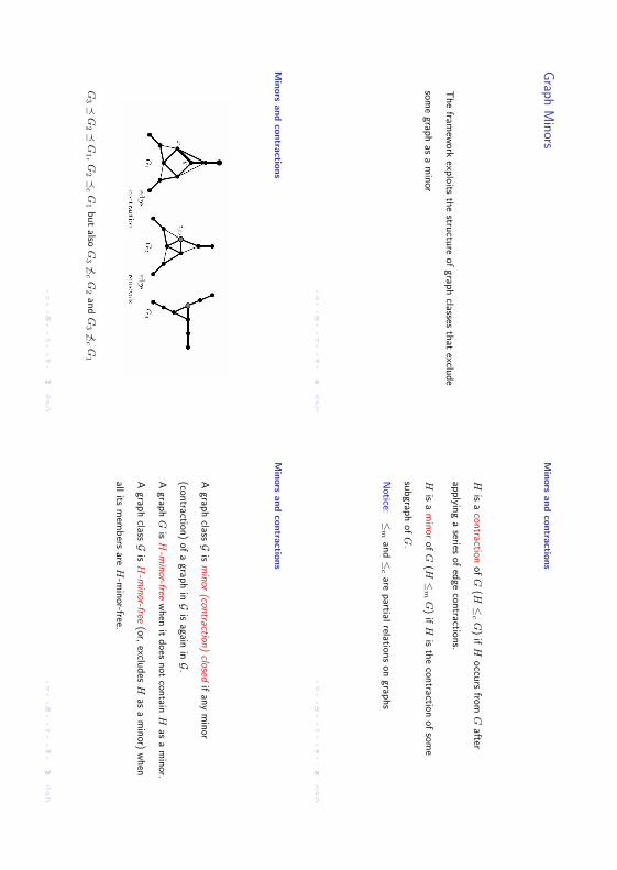
His

acon

tractionof

G(H

≤cG

)if

Hoccu

rsfrom

Gafter

applyin

ga

seriesof

edge

contraction

s.

His

am

inor

ofG

(H≤

mG

)if

His

the

contraction

ofsom

e

subgrap

hof

G.

Notice:

≤m

and≤

care

partial

relations

ongrap

hs

Min

ors

and

contra

ctions

G3

G2

G1 ,

G2

cG

1but

alsoG

3 6cG

2an

dG

3 6cG

1

Min

ors

and

contra

ctions

Agrap

hclassG

ism

inor

(contraction

)closed

ifan

ym

inor

(contraction

)of

agrap

hinG

isagain

inG.

Agrap

hG

isH

-min

or-freew

hen

itdoes

not

contain

Has

am

inor.

Agrap

hclassG

isH

-min

or-free(or,

excludes

Has

am

inor)

when

allits

mem

bers

areH

-min

or-free.

Exam

plesof

H-m

inor-freeclasses

Forests:

K3

O

uterp

lanar

Grap

hs:

K2,3 ,

K4

Plan

arG

raphs:

K3,3 ,

K5

Lin

k-freeG

raphs:

7grap

hs

(X-Y

transform

ations

ofK

6 )

G

raphs

ofth

eprojective

plan

e:103

graphs

Graph

Minor

theorem

Rob

ertson&

Seym

our

(1986–2004):

Theorem

(Grap

hs

Min

orT

heorem

)

Grap

hs

arewell-q

uasi-ord

eredby

the

min

orrelation≤

m.

Con

sequen

ce:every

min

orclosed

graph

classGhas

afinite

set

ofm

inim

alexclu

ded

min

ors.

Graph

Minor

theorem

Grap

hs

Min

orT

heorem

isnot

used

inou

rtu

torial.H

owever,w

e

need

tools

createdby

Rob

erston-S

eymou

rin

order

toprof

this

theorem

.

Main

tool:

Branch

Decom

positions

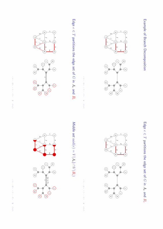
Defi

nition

Abran

chdecom

position

ofa

graph

G=(V

,E)

isa

tuple(T

,µ)

where

T

isa

treew

ithdegree

3for

allin

ternal

nodes.

µ

isa

bijection

betw

eenth

eleaves

ofT

and

E(G).

Exam

pleof

Branch

Decom

position

8

46

13

ab

fg

cd

m

hi

jk

l

j

l

bm

k g

c

ad

fhi

c5

7

2

Edge

e∈T

partitionsthe

edgeset

ofG

inA

eand

Be

8

46

13

ab

fg

cd

m

hi

jk

l

j

l

bm

k g

c

ad

fhi

c5

7

2

Edge

e∈T

partitionsthe

edgeset

ofG

inA

eand

Be

8

46

13

ab

fg

cd

m

hi

jk

l

j

l

bm

k g

c

ad

fhi

ec

5

7

2

Middle

setm

id(e)

=V

(Ae )∩

V(B

e )

8

46

13

ab

fg

cd

m

hi

jk

l

j

l

bm

k g2,5

,7

c

ad

fhi

ec

5

7

2

Branchw

idth

T

he

wid

thof

abran

chdecom

position

ismax

e∈T |m

id(e)|.

T

he

branch

wid

thof

agrap

hG

isth

em

inim

um

wid

thover

all

branch

decom

position

sof

G.

Exercises

W

hat

isth

ebran

chw

idth

ofa

tree?

Com

plete

graph

onn

vertices?

(ℓ×

ℓ)-grid?

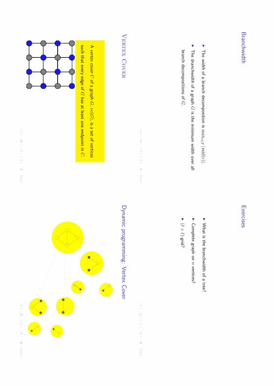
Vertex

Cover

Avertex

coverC

ofa

graph

G,vc(G

),is

aset

ofvertices

such

that

everyed

geof

Ghas

atleast

one

endpoin

tin

C.

Dynam

icprogram

ming:

Vertex

Cover

Dynam

icprogram

ming:

Vertex

Cover

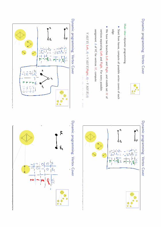
Main

idea—

dyn

amic

programm

ing.

Start

fromleaves,

compute

allpossib

levertex

coversof

each

edge

W

ehave

two

branch

esLeft

and

Righ

t,an

dm

iddle

setM

of

verticessep

arating

Left

and

Righ

t.For

everypossib

le

assignm

ent

Aof

VC

forvertices

M,com

pute

VA

LU

E(

Left,A

)+

VA

LU

E(R

ight,A

)−V

AL

UE(A)

Dynam

icprogram

ming:

Vertex

Cover

Dynam

icprogram

ming:

Vertex

Cover

Dynam

icprogram

ming:

Vertex

Cover

Dynam

icprogram

ming:

Vertex

Cover

Dynam

icprogram

ming:

Vertex

Cover

Dynam

icprogram

ming:

Vertex

Cover

Dynam

icprogram

ming:

Vertex

Cover

Let

ℓ=

bw(G)

and

m=|E(G)|.

Runnin

gtim

e:size

ofevery

table

form

iddle

setis

O(2

ℓ).

To

compute

anew

table:

O(2

2ℓ)

N

um

ber

ofstep

sO(m

)

Total

runnin

gtim

e:O(2

2ℓm).

Dynam

icprogram

ming:

Vertex

Cover

Exercise

Try

toim

proveth

eru

nnin

gtim

e,say

toO(2

1.5

ℓm).

Grid

Theorem

Theorem

(Rob

ertson,Seym

our&

Thom

as,1994)

Let

ℓ≥1

be

anin

teger.Every

plan

argrap

hof

branch

wid

th≥4ℓ

contain

sℓ

asa

min

or.

Grid

Theorem

:Sketch

ofthe

proof

The

proof

isbased

onM

enger’s

Theorem

Theorem

(Menger

1927)

Let

Gbe

afinite

undirected

graph

and

xan

dy

two

non

adjacen

t

vertices.T

he

sizeof

the

min

imum

vertexcu

tfor

xan

dy

(the

min

imum

num

ber

ofvertices

whose

removal

discon

nects

xan

dy)

iseq

ual

toth

em

aximum

num

ber

ofpairw

isevertex-d

isjoint

path

s

fromx

toy.

Grid

Theorem

:Sketch

ofthe

proof

Let

Gbe

aplan

egrap

hth

athas

no(ℓ×

ℓ)-gridas

am

inor.

WE

ST

NO

RT

H

SOU

TH

EA

ST

Grid

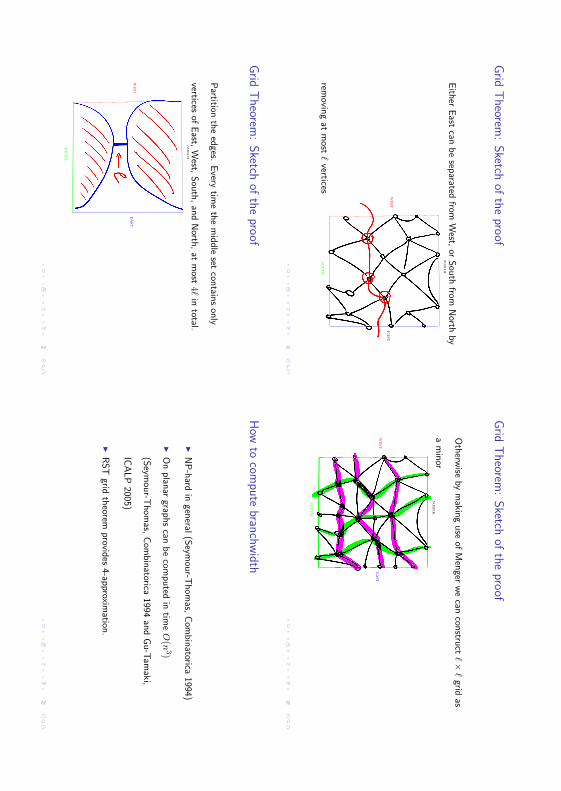
Theorem

:Sketch

ofthe

proof

Eith

erEast

canbe

separated

fromW

est,or

Sou

thfrom

North

by

removin

gat

most

ℓvertices

WE

ST

NO

RT

H

SOU

TH

EA

ST

Grid

Theorem

:Sketch

ofthe

proof

Oth

erwise

bym

aking

use

ofM

enger

we

cancon

struct

ℓ×ℓ

gridas

am

inor

WE

ST

NO

RT

H

SOU

TH

EA

ST

SOU

TH

Grid

Theorem

:Sketch

ofthe

proof

Partition

the

edges.

Every

time

the

mid

dle

setcon

tains

only

verticesof

East,

West,

Sou

th,an

dN

orth,at

most

4ℓ

intotal.

WE

ST

NO

RT

H

SOU

TH

EA

ST

How

tocom

putebranchw

idth

N

P-h

ardin

general

(Seym

our-T

hom

as,Com

bin

atorica1994)

O

nplan

argrap

hs

canbe

computed

intim

eO(n

3)

(Seym

our-T

hom

as,Com

bin

atorica1994

and

Gu-T

amaki,

ICA

LP

2005)

RST

gridth

eoremprovid

es4-ap

proximation

.

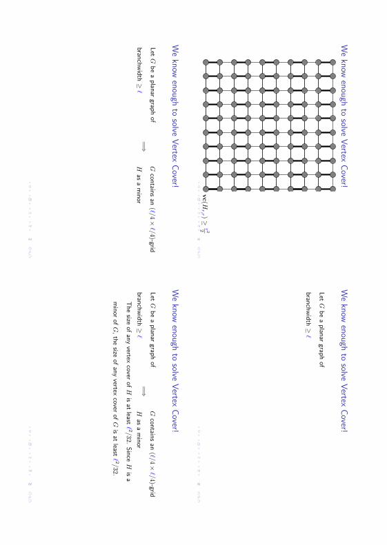
We

knowenough

tosolve

Vertex

Cover!

vc(Hr,r )≥

r22

We

knowenough

tosolve

Vertex

Cover!

Let

Gbe

aplan

argrap

hof

branch

wid

th≥ℓ

We

knowenough

tosolve

Vertex

Cover!

Let

Gbe

aplan

argrap

hof

branch

wid

th≥ℓ

=⇒G

contain

san

(ℓ/4×ℓ/4)-grid

Has

am

inor

We

knowenough

tosolve

Vertex

Cover!

Let

Gbe

aplan

argrap

hof

branch

wid

th≥ℓ

=⇒G

contain

san

(ℓ/4×ℓ/4)-grid

Has

am

inor

The

sizeof

any

vertexcover

ofH

isat

leastℓ2/32.

Sin

ceH

isa

min

orof

G,th

esize

ofan

yvertex

coverof

Gis

atleast

ℓ2/32.

We

knowenough

tosolve

Vertex

Cover!

Let

Gbe

aplan

argrap

hof

branch

wid

th≥ℓ

=⇒G

contain

san

(ℓ/4×ℓ/4)-grid

Has

am

inor

The

sizeof

any

vertexcover

ofH

isat

leastℓ2/32.

Sin

ceH

isa

min

orof

G,th

esize

ofan

yvertex

coverof

Gis

atleast

ℓ2/32.

WIN

/WIN

Ifk

<ℓ2/32,

we

say“N

O”

Ifk≥

ℓ2/32,

then

we

do

DP

intim

e

O(2

2ℓm)=

O(2

O( √

k)m).

Challenges

to

disc

uss

H

owto

generalize

the

idea

towork

foroth

erparam

eters?

D

oes

not

work

forD

omin

ating

Set.

Why?

Is

plan

arityessen

tial?

D

ynam

icprogram

min

g.D

oes

MSO

Lhelp

shere?

Param

eters

Aparam

eterP

isan

yfu

nction

map

pin

ggrap

hs

tonon

negative

integers.

The

param

eterizedprob

lemasso

ciatedw

ithP

asks,for

some

fixed

k,w

heth

erfor

agiven

graph

G,P(G)≤

k(for

min

imization

)an

dP(G)≥

k(for

maxim

izationprob

lem).

We

say

that

aparam

eterP

isclosed

under

taking

ofm

inors/con

tractions

(or,briefl

y,m

inor/con

tractionclosed

)if

forevery

graph

H,H

G

/H

cG

implies

that

P(H

)≤P(G).

Examples

of

parameters:

k-V

ertex

Cover

Avertex

coverC

ofa

graph

G,vc(G

),is

aset

ofvertices

such

that

everyed

geof

Ghas

atleast

one

endpoin

tin

C.

The

k-V

ertex

Cover

problem

isto

decid

e,given

a

graph

Gan

da

positive

integer

k,w

heth

erG

has

avertex

coverof

sizek.

k-V

ertex

Cover

k-V

ertex

Cover

isclosed

under

taking

min

ors.

Examples

of

parameters:

k-D

omin

atin

gse

t

Adom

inatin

gset

Dof

agrap

hG

isa

setof

verticessu

ch

that

everyvertex

outsid

eD

isad

jacent

toa

vertexof

D.

The

k-D

omin

atin

gSet

problem

isto

decid

e,given

a

graph

Gan

da

positive

integer

k,w

heth

erG

has

a

dom

inatin

gset

ofsize

k.

k-D

omin

atin

gse

t

k-D

omin

atin

gse

tis

not

closedunder

taking

min

ors.H

owever,

itis

closedunder

contraction

ofed

ges.

(Not

exactlyrelated

tothis

tutorialbut

worth

tobe

mentioned)

By

Rob

ertson-S

eymou

rth

eory,every

min

orclosed

param

eter

problem

isFPT

.

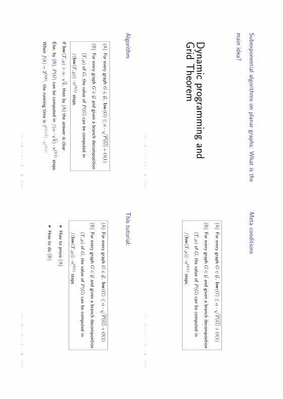
Sub

exponential

algorithms

onplanar

graphs:W

hatis

the

main

idea?

Dynam

icprogram

ming

andG

ridT

heorem

Meta

conditions

(A)

For

everygrap

hG∈G,

bw(G)≤

α· √P(G)+

O(1)

(B)

For

everygrap

hG∈G

and

givena

branch

decom

position

(T,µ)

ofG

,th

evalu

eof

P(G)

canbe

computed

in

f(bw(T

,µ))·nO

(1)

steps.

Algorithm

(A)

For

everygrap

hG∈G,

bw(G)≤

α· √P(G)+

O(1)

(B)

For

everygrap

hG∈G

and

givena

branch

decom

position

(T,µ)

ofG

,th

evalu

eof

P(G)

canbe

computed

in

f(bw(T

,µ))·nO

(1)

steps.

Ifbw(T

,µ)>

α· √k,th

enby

(A)

the

answ

eris

clear

Else,

by(B

),P(G)

canbe

computed

inf(α· √

k)·nO

(1)

steps.

When

f(k)=2

O(k

),th

eru

nnin

gtim

eis2

O( √

k)·

nO

(1)

This

tutorial:

(A)

For

everygrap

hG∈G,

bw(G)≤

α· √P(G)+

O(1)

(B)

For

everygrap

hG∈G

and

givena

branch

decom

position

(T,µ)

ofG

,th

evalu

eof

P(G)

canbe

computed

in

f(bw(T

,µ))·nO

(1)

steps

H

owto

prove(A

)

H

owto

do

(B)

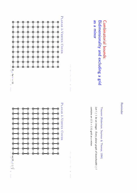
Com

binatorialbounds:

Bidim

ensionalityand

excludinga

gridas

am

inor

Rem

inder

Theorem

(Rob

ertson,Seym

our&

Thom

as,1994)

Let

ℓ≥1

be

anin

teger.Every

plan

argrap

hof

branch

wid

th≥ℓ

contain

san

(ℓ/4×ℓ/4)-grid

asa

min

or.

Planar

k-V

ertex

Cover

Hr,r

forr=10

Planar

k-V

ertex

Cover

vc(Hr,r )≥

r22

Planar

k-V

ertex

Cover

Let

Gbe

aplan

argrap

hof

branch

wid

th≥ℓ

Planar

k-V

ertex

Cover

Let

Gbe

aplan

argrap

hof

branch

wid

th≥ℓ

=⇒G

contain

san

(ℓ/4×ℓ/4)-grid

Has

am

inor

Planar

k-V

ertex

Cover

Let

Gbe

aplan

argrap

hof

branch

wid

th≥ℓ

=⇒G

contain

san

(ℓ/4×ℓ/4)-grid

Has

am

inor

The

sizeof

any

vertexcover

ofH

isat

leastℓ2/32.

Sin

ceH

isa

min

orof

G,th

esize

ofan

yvertex

coverof

Gis

atleast

ℓ2/32.

Planar

k-V

ertex

Cover

Let

Gbe

aplan

argrap

hof

branch

wid

th≥ℓ

=⇒G

contain

san

(ℓ/4×ℓ/4)-grid

Has

am

inor

The

sizeof

any

vertexcover

ofH

isat

leastℓ2/32.

Sin

ceH

isa

min

orof

G,th

esize

ofan

yvertex

coverof

Gis

atleast

ℓ2/32.

Con

clusion

:Prop

erty(A

)hold

sfor

α=4 √

2,i.e.

bw(G)≤

4 √2 √

vc(G).

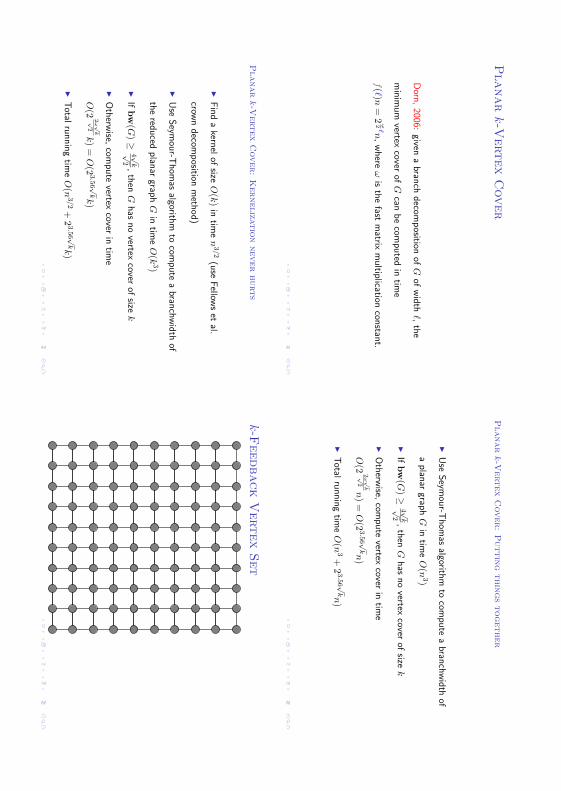
Planar

k-V

ertex

Cover

Dorn

,2006:

givena

branch

decom

position

ofG

ofw

idth

ℓ,th

e

min

imum

vertexcover

ofG

canbe

computed

intim

e

f(ℓ)n=2

ω2ℓn

,w

here

ωis

the

fastm

atrixm

ultip

licationcon

stant.

Planar

k-V

ertex

Cover:

Puttin

gthin

gs

together

U

seSeym

our-T

hom

asalgorith

mto

compute

abran

chw

idth

of

aplan

argrap

hG

intim

eO(n

3)

If

bw(G)≥

4 √k

√2

,th

enG

has

no

vertexcover

ofsize

k

O

therw

ise,com

pute

vertexcover

intim

e

O(2

2ω √

k√

2n)

=O(2

3.5

6 √kn)

Total

runnin

gtim

eO(n

3+23.5

6 √kn)

Planar

k-V

ertex

Cover:

Kerneliz

atio

nnever

hurts

Fin

da

kernel

ofsize

O(k)

intim

en

3/2

(use

Fellow

set

al.

crown

decom

position

meth

od)

U

seSeym

our-T

hom

asalgorith

mto

compute

abran

chw

idth

of

the

reduced

plan

argrap

hG

intim

eO(k

3)

If

bw(G)≥

4 √k

√2

,th

enG

has

no

vertexcover

ofsize

k

O

therw

ise,com

pute

vertexcover

intim

e

O(2

2ω √

k√

2k)=

O(2

3.5

6 √kk)

Total

runnin

gtim

eO(n

3/2+23.5

6 √kk)

k-F

eedback

Vertex

Set

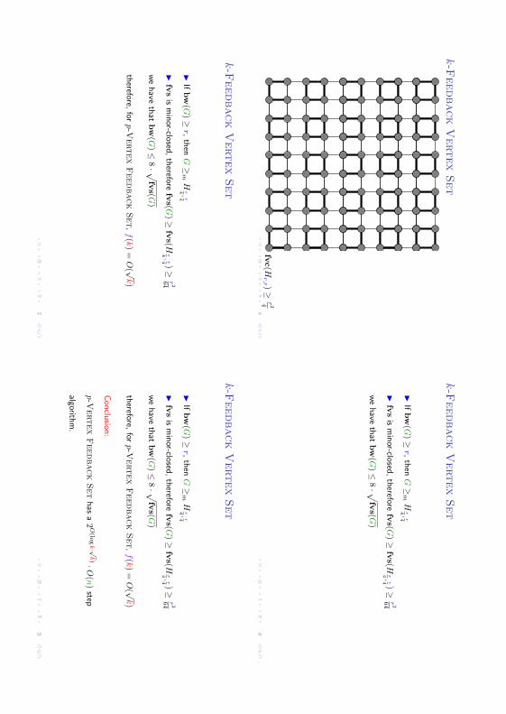
k-F

eedback

Vertex

Set

fvc(Hr,r )≥

r24

k-F

eedback

Vertex

Set

If

bw(G)≥

r,th

enG≥

mH

r4,r4

fv

sis

min

or-closed,th

ereforefv

s(G)≥

fvs(H

r4,r4 )≥

r2

64

we

have

that

bw(G)≤

8· √fv

s(G)

k-F

eedback

Vertex

Set

If

bw(G)≥

r,th

enG≥

mH

r4,r4

fv

sis

min

or-closed,th

ereforefv

s(G)≥

fvs(H

r4,r4 )≥

r2

64

we

have

that

bw(G)≤

8· √fv

s(G)

therefore,

forp-V

ertex

Feedback

Set,f(k)

=O( √

k)

k-F

eedback

Vertex

Set

If

bw(G)≥

r,th

enG≥

mH

r4,r4

fv

sis

min

or-closed,th

ereforefv

s(G)≥

fvs(H

r4,r4 )≥

r2

64

we

have

that

bw(G)≤

8· √fv

s(G)

therefore,

forp-V

ertex

Feedback

Set,f(k)

=O( √

k)

Con

clusion

:

p-V

ertex

Feedback

Set

has

a2

O(lo

gk· √

k)·O

( n)step

algorithm

.

Planar

k-D

omin

atin

gSet

Can

we

proceed

byth

esam

eargu

men

tsw

ithPlanar

k-D

omin

atin

gSet?

Planar

k-D

omin

atin

gSet

Can

we

proceed

byth

esam

eargu

men

tsw

ithPlanar

k-D

omin

atin

gSet?

Oop

s!H

ereis

aprob

lem!

Dom

inatin

gset

isnot

min

orclosed

!

Planar

k-D

omin

atin

gSet

Can

we

proceed

byth

esam

eargu

men

tsw

ithPlanar

k-D

omin

atin

gSet?

Oop

s!H

ereis

aprob

lem!

Dom

inatin

gset

isnot

min

orclosed

!

How

ever,dom

inatin

gset

isclosed

under

contraction

Planar

k-D

omin

atin

gSet

Hr,r

forr=10

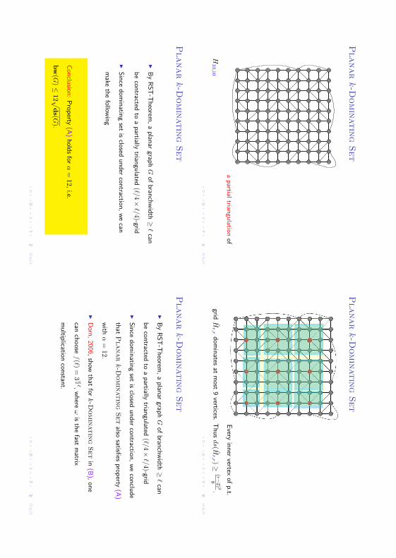
Planar

k-D

omin

atin

gSet

apartial

triangu

lationof

H10,1

0

Planar

k-D

omin

atin

gSet

Every

inner

vertexof

p.t.

gridH

r,r

dom

inates

atm

ost9

vertices.T

hus

ds(H

r,r )≥

(r−2)2

9.

Planar

k-D

omin

atin

gSet

B

yRST

-Theorem

,a

plan

argrap

hG

ofbran

chw

idth≥

ℓcan

be

contracted

toa

partially

triangu

lated(ℓ/4×

ℓ/4)-grid

Sin

cedom

inatin

gset

isclosed

under

contraction

,we

can

make

the

followin

g

Con

clusion

:Prop

erty(A

)hold

sfor

α=12,

i.e.

bw(G)≤

12 √ds(G

).

Planar

k-D

omin

atin

gSet

B

yRST

-Theorem

,a

plan

argrap

hG

ofbran

chw

idth≥

ℓcan

be

contracted

toa

partially

triangu

lated(ℓ/4×

ℓ/4)-grid

Sin

cedom

inatin

gset

isclosed

under

contraction

,we

conclu

de

that

Planar

k-D

omin

atin

gSet

alsosatisfi

esprop

erty(A

)

with

α=12.

D

orn,2006,

show

that

fork-D

omin

atin

gSet

in(B

),on

e

canch

oose

f(ℓ)=3

ω2ℓ,

where

ωis

the

fastm

atrix

multip

licationcon

stant.

Planar

k-D

omin

atin

gSet

B

yRST

-Theorem

,a

plan

argrap

hG

ofbran

chw

idth≥

ℓcan

be

contracted

toa

partially

triangu

lated(ℓ/4×

ℓ/4)-grid

Sin

cedom

inatin

gset

isclosed

under

contraction

,we

conclu

de

that

Planar

k-D

omin

atin

gSet

alsosatisfi

esprop

erty(A

)

with

α=12.

D

orn,2006,

show

that

fork-D

omin

atin

gSet

in(B

),on

e

canch

oose

f(ℓ)=3

ω2ℓ,

where

ωis

the

fastm

atrix

multip

licationcon

stant.

Con

clusion

:Planar

k-D

omin

atin

gSet

canbe

solvedin

time

O(n

3+222.6 √

kn)

Bidim

ensionality:T

hem

ainidea

Ifth

egrap

hparam

eteris

closedunder

taking

min

orsor

contraction

s,th

eon

lyth

ing

need

edfor

the

proof

branch

wid

th/p

arameter

bou

nd

isto

understan

dhow

this

param

eter

beh

aveson

a(p

artiallytrian

gulated

)grid

.

Bidim

ensionality:D

emaine,

FF,H

ajiaghayi,T

hilikos,2005

Defi

nition

Aparam

eterP

ism

inor

bid

imen

sional

with

den

sityδ

if

1.P

isclosed

under

taking

ofm

inors,

and

2.for

the(r×

r)-gridR

,P(R)=(δr)

2+

o((δr)2).

Bidim

ensionality:D

emaine,

FF,H

ajiaghayi,T

hilikos,2005

Defi

nition

Aparam

eterP

iscalled

contraction

bid

imen

sional

with

den

sityδ

if

1.P

isclosed

under

contraction

s,

2.for

any

partially

triangu

lated(r×

r)-gridR

,

P(R)=(δ

Rr)

2+

o((δRr)

2),an

d

3.δ

isth

esm

allestδR

amon

gall

paritally

triangu

lated

(r×r)-grid

s.

Bidim

ensionality

Lem

ma

IfP

isa

bid

imen

sional

param

eterw

ithden

sityδ

then

Psatisfi

es

property

(A)

forα=4/δ,

onplan

argrap

hs.

Pro

of.

Let

Rbe

an(r×

r)-grid.

P(R)≥

(δRr)

2.

IfG

contain

sR

asa

min

or,th

enbw(G)≤

4r≤

4/δ √P(G).

Exam

plesof

bidimensional

problems

Vertex

cover

Dom

inatin

gSet

Indep

enden

tSet

(k,r)-cen

ter

Feed

back

Vertex

Set

Min

imum

Maxim

alM

atchin

g

Plan

arG

raph

TSP

Lon

gestPath

...

How

toextend

bidimensionality

tom

oregeneral

graph

classes?

W

eneed

excludin

ggrid

theorem

s(su

fficien

tfor

min

orclosed

param

eters)

For

contraction

closedparam

eterswe

have

tobe

more

careful

Bounded

genusgraphs:

Dem

aine,FF,H

ajiaghayi,T

hilikos,

2005Theorem

IfG

isa

graph

ofgen

us

atm

ostγ

with

branch

wid

thm

oreth

anr,

then

Gcon

tains

a(r/4(γ

+1)×

r/4(γ+1))-grid

asa

min

or.

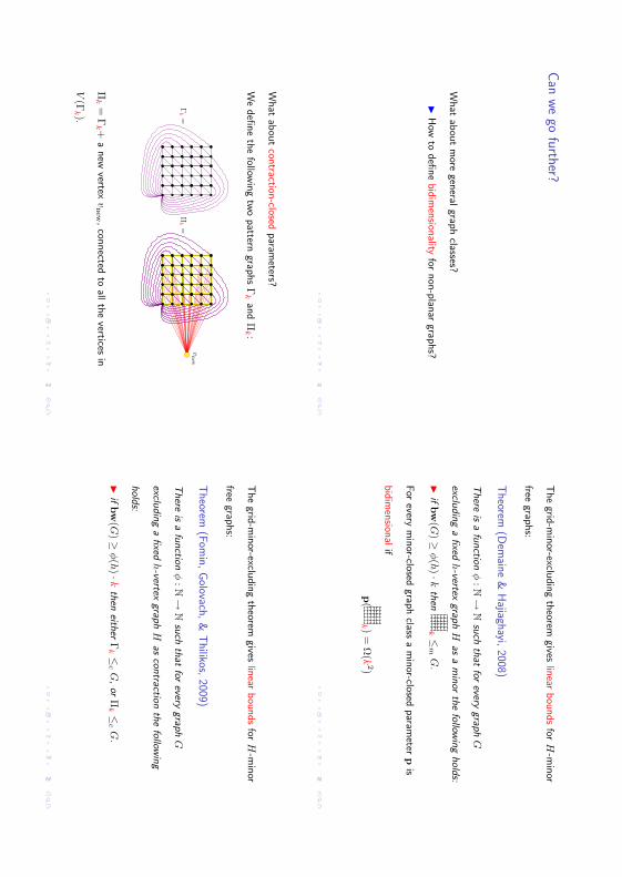
Can

we

gofurther?

What

abou

tm

oregen

eralgrap

hclasses?

H

owto

defi

ne

bid

imen

sionality

fornon

-plan

argrap

hs?

The

grid-m

inor-exclu

din

gth

eoremgives

linear

bou

nds

forH

-min

or

freegrap

hs:

Theorem

(Dem

aine&

Hajiaghayi,

2008)

There

isa

function

φ:N

→N

such

that

forevery

graph

G

excludin

ga

fixed

h-vertex

graph

Has

am

inor

the

followin

ghold

s:

if

bw(G)≥

φ(h)·k

then

k ≤m

G.

For

everym

inor-closed

graph

classa

min

or-closedparam

eterp

is

bid

imen

sional

if

p(

k )=Ω(k

2)

What

abou

tcon

traction-closed

param

eters?

We

defi

ne

the

followin

gtw

opattern

graphsΓ

kan

dΠ

k :

Πk

=Γ

k=

vnew

Πk=Γ

k +a

new

vertexvnew

,con

nected

toall

the

verticesin

V(Γ

k ).

The

grid-m

inor-exclu

din

gth

eoremgives

linear

bou

nds

forH

-min

or

freegrap

hs:

Theorem

(Fom

in,G

olovach,&

Thilikos,

2009)

There

isa

function

φ:N

→N

such

that

forevery

graph

G

excludin

ga

fixed

h-vertex

graph

Has

contraction

the

followin

g

hold

s:

if

bw(G)≥

φ(h)·k

then

eitherΓ

k ≤cG

,orΠ

k ≤cG

.

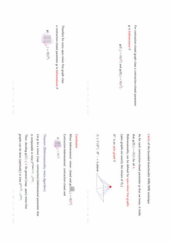
For

contraction

-closedgrap

hclass

acon

traction-closed

param

eter

pis

bid

imen

sional

if

p(Γ

k )=Ω(k

2)an

dp(Π

k )=Ω(k

2).

Lim

itsof

the

bou

nded

branch

wid

thW

IN/W

INtech

niq

ue

As

foreach

contraction

-closedparam

eterp

that

we

know

,it

hold

s

that

p(Π

k )=

O(1)

forall

k,

Bid

imen

sionality

canbe

defi

ned

forap

ex-min

orfree

graphs

(apex

graphs

areexactly

the

min

orsofΠ

k )

H∗

isan

apex

graph

if

∃v∈

V(H

∗):H∗−

vis

plan

ar

Therefore

forevery

apex-m

inor

freegrap

hclass

acon

traction-closed

param

eterp

isbid

imen

sional

if

p(

k )=

Ω(k

2)

Conclusion

Min

orbid

imen

sional:

min

or-closed

and

p(

k )=Ω(k

2)

Con

traction-b

idim

ension

al:con

traction-closed

and

p(

k )=

Ω(k

2)

Theorem

(Bidim

ensionalitym

eta-algorithm)

Let

pbe

am

inor

(resp.

contraction

)-bid

imen

sional

param

eterth

at

iscom

putab

lein

time2

O(b

w( G

))·n

O(1

).

Then

,decid

ing

p(G)≤

kfor

general

(resp.

apex)

min

or-free

graphs

canbe

don

e(op

timally)

intim

e2

O( √

k)· n

O(1

).

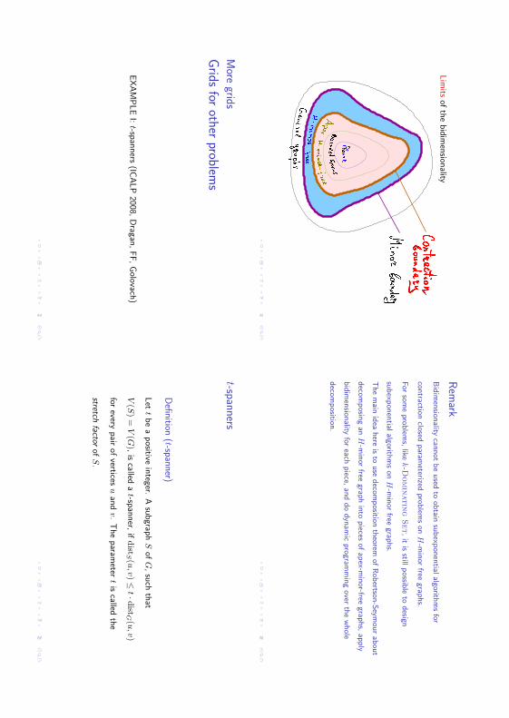
Lim

itsof

the

bid

imen

sionality

Rem

ark

Bid

imen

sionality

cannot

be

used

toob

tainsu

bexp

onen

tialalgorith

ms

for

contraction

closedparam

eterizedprob

lems

onH

-min

orfree

graphs.

For

some

problem

s,like

k-D

omin

atin

gSet,it

isstill

possib

leto

design

subexp

onen

tialalgorith

ms

onH

-min

orfree

graphs.

The

main

idea

here

isto

use

decom

position

theorem

ofRob

ertson-S

eymou

rab

out

decom

posin

gan

H-m

inor

freegrap

hin

topieces

ofap

ex-min

or-freegrap

hs,

apply

bid

imen

sionality

foreach

piece,

and

do

dyn

amic

programm

ing

overth

ew

hole

decom

position

.

More

grids

Grids

forother

problems

EX

AM

PLE

I:t-sp

anners

(ICA

LP

2008,D

ragan,FF,G

olovach)

t-spanners

Defi

nition(t-spanner)

Let

tbe

apositive

integer.

Asu

bgrap

hS

ofG

,su

chth

at

V(S)=

V(G),

iscalled

at-sp

anner,

ifdist

S (u,v)≤

t·distG(u

,v)

forevery

pair

ofvertices

uan

dv.

The

param

etert

iscalled

the

stretchfactor

ofS

.

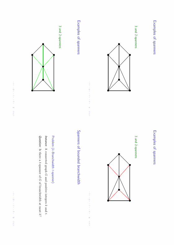
Exam

plesof

spanners

3and

2-spanners

Exam

plesof

spanners

3and

2-spanners

Exam

plesof

spanners

3and

2-spanners

Spanners

ofbounded

branchwidth

Problem

(k-B

ranchwidth

t-spanner)

Instan

ce:Aconnected

graphGand

positiveintegers

kand

t.

Question

:Isthere

at-spanner

ofGofbranchw

idthatmost

k?

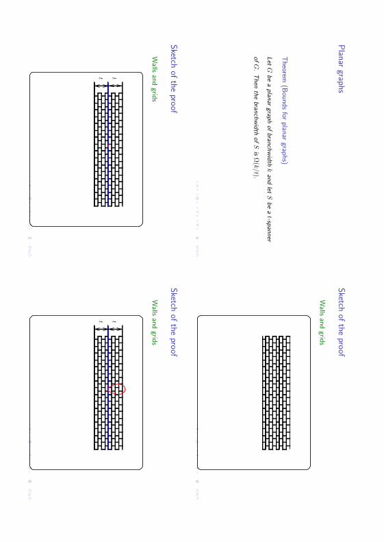
Planar

graphs

Theorem

(Bounds

forplanar

graphs)

Let

Gbe

aplan

argrap

hof

branch

wid

thk

and

letS

be

at-sp

anner

ofG

.T

hen

the

branch

wid

thof

SisΩ(k

/t).

Sketch

ofthe

proof

Walls

andgrids

Sketch

ofthe

proof

Walls

andgrids

tt

Sketch

ofthe

proof

Walls

andgrids

tt

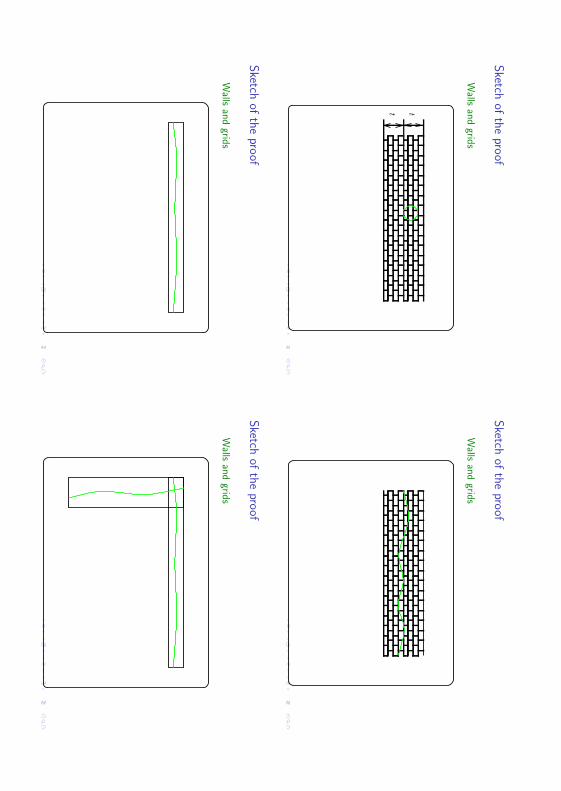
Sketch

ofthe

proof

Walls

andgrids

tt

Sketch

ofthe

proof

Walls

andgrids

Sketch

ofthe

proof

Walls

andgrids

Sketch

ofthe

proof

Walls

andgrids

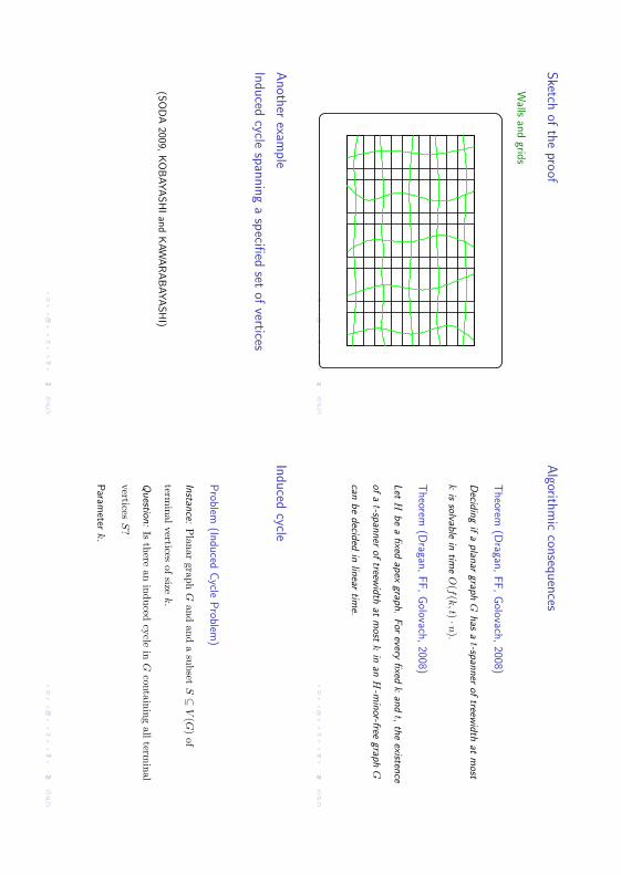
Sketch

ofthe

proof

Walls

andgrids

Algorithm

icconsequences

Theorem

(Dragan,

FF,G

olovach,2008)

Decid

ing

ifa

plan

argrap

hG

has

at-sp

anner

oftreew

idth

atm

ost

kis

solvable

intim

eO(f(k

,t)·n).

Theorem

(Dragan,

FF,G

olovach,2008)

Let

Hbe

afixed

apex

graph.

For

everyfixed

kan

dt,

the

existence

ofa

t-span

ner

oftreew

idth

atm

ostk

inan

H-m

inor-free

graph

G

canbe

decid

edin

linear

time.

Another

example

Inducedcycle

spanninga

specifi

edset

ofvertices

(SO

DA

2009,KO

BAYA

SH

Ian

dK

AW

ARA

BAYA

SH

I)

Inducedcycle

Problem

(InducedCycle

Problem

)

Instan

ce:Planar

graphGand

andasubset

S⊆

V(G)of

terminal

verticesofsize

k.

Question

:Isthere

aninduced

cyclein

Gcontaining

allterm

inal

verticesS?

Param

eterk.

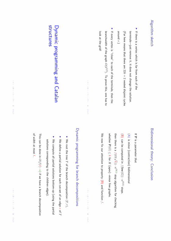
Algorithm

sketch

If

there

isa

vertexw

hich

isfar

fromeach

ofth

e

termin

als—ju

strem

oveit,

itdoes

not

chan

geth

esolu

tion.

(Far

here

mean

sth

atth

ereare

22k+2

nested

disjoin

tcycles

around

v.)

If

everyvertex

is“close”

toeach

ofth

eterm

inals,

then

the

branch

wid

thof

the

graph

O(k

3/2).

To

proveth

is,on

ehas

to

look

atth

egrid

!

Bidim

ensionaltheory:

Conclusion

IfP

isa

param

eterth

at

(A)

ism

inor

(contraction

)bid

imen

sional

(B)

canbe

computed

inf(b

w(G))·n

O(1

)step

s.

then

there

isa

f(O( √

k))·n

O( 1

)step

algorithm

forch

ecking

wheth

erP(G)≤

kfor

H(ap

ex)-m

inor

freegrap

hs.

We

now

fix

our

attention

toprop

erty(B

)an

dfu

nction

f.

Dynam

icprogram

ming

andCatalan

structures

Dynam

icprogram

ming

forbranch

decompositions

W

ero

otth

etree

Tof

the

branch

decom

position

(T,τ),

W

edefi

ne

apartial

solution

foreach

cut-set

ofan

edge

eof

T

W

ecom

pute

allpartial

solution

sbottom

-up

(usin

gth

epartial

solution

scorresp

ondin

gto

the

child

rened

ges).

This

canbe

don

ein

O(f( ℓ)·n)

ifwe

have

abran

chdecom

position

ofw

idth

atm

ostℓ.

Dynam

icprogram

ming

forbranch

decompositions

W

ero

otth

etree

Tof

the

branch

decom

position

(T,τ),

W

edefi

ne

apartial

solution

foreach

cut-set

ofan

edge

eof

T

W

ecom

pute

allpartial

solution

sbottom

-up

(usin

gth

epartial

solution

scorresp

ondin

gto

the

child

rened

ges).

This

canbe

don

ein

O(f( ℓ)·n)

ifwe

have

abran

chdecom

position

ofw

idth

atm

ostℓ.

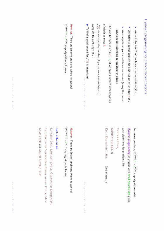
f( ℓ)dep

ends

onth

enum

ber

ofpartial

solution

swe

have

to

compute

foreach

edge

ofT

.

To

find

ago

od

bou

nd

forf(ℓ)

isim

portan

t!

For

man

yprob

lems,2

O(b

w(G

))· nO

(1)

stepalgorith

ms

exist.

Dyn

amic

programm

ing

ongrap

hs

with

small

branch

wid

thgives

such

algorithm

sfor

problem

slike

Vertex

Cover,

Domin

atin

gSet,or

Edge

Domin

atin

gSet,

(and

others...)

How

ever:T

here

are(m

any)

problem

sw

here

no

general

2O

(bw

(G))· n

O(1

)step

algorithm

iskn

own.

How

ever:T

here

are(m

any)

problem

sw

here

no

general

2O

(bw

(G))· n

O(1

)step

algorithm

iskn

own.

Such

problem

sare

Longest

Path,Longest

Cycle,C

onnected

Domin

atin

g

Set,Feedback

Vertex

Set,H

amilt

onia

nC

ycle,M

ax

Leaf

Tree

and

Graph

Metric

TSP

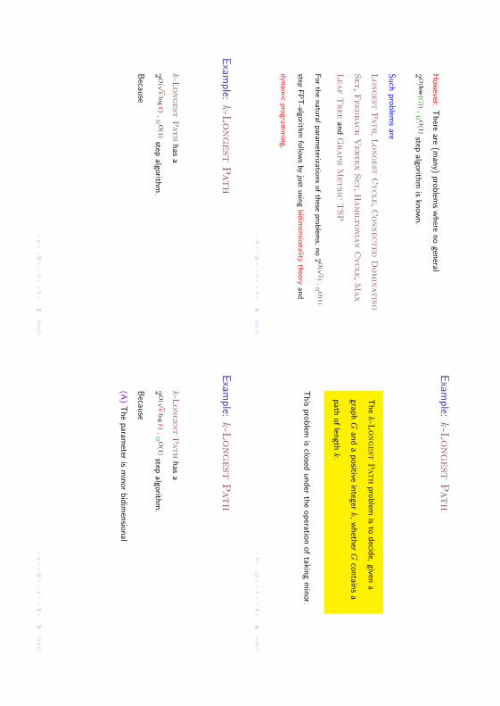
How

ever:T

here

are(m

any)

problem

sw

here

no

general

2O

(bw

(G))·n

O(1

)step

algorithm

iskn

own.

Such

problem

sare

Longest

Path,Longest

Cycle,C

onnected

Domin

atin

g

Set,Feedback

Vertex

Set,H

amilt

onia

nC

ycle,M

ax

Leaf

Tree

and

Graph

Metric

TSP

For

the

natu

ralparam

eterizations

ofth

eseprob

lems,

no2

O( √

k)·

nO

(1)

stepFPT

-algorithm

follows

byju

stusin

gbid

imen

sionality

theory

and

dyn

amic

programm

ing.

Exam

ple:k-L

ongest

Path

The

k-L

ongest

Path

problem

isto

decid

e,given

a

graph

Gan

da

positive

integer

k,w

heth

erG

contain

sa

path

oflen

gthk.

This

problem

isclosed

under

the

operation

oftakin

gm

inor.

Exam

ple:k-L

ongest

Path

k-L

ongest

Path

has

a

2O

( √k·lo

gk)·n

O(1

)step

algorithm

.

Becau

se

Exam

ple:k-L

ongest

Path

k-L

ongest

Path

has

a

2O

( √k·lo

gk)·n

O(1

)step

algorithm

.

Becau

se

(A)

The

param

eteris

min

orbid

imen

sional

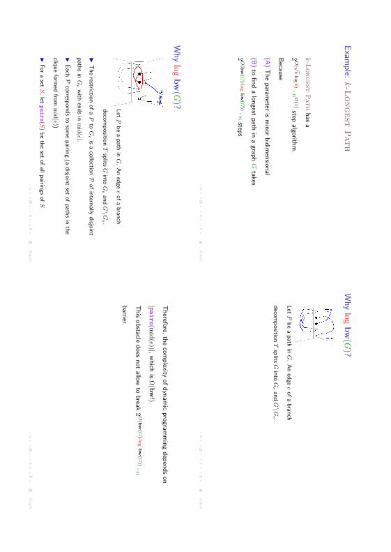
Exam

ple:k-L

ongest

Path

k-L

ongest

Path

has

a

2O

( √k·lo

gk)· n

O(1

)step

algorithm

.

Becau

se

(A)

The

param

eteris

min

orbid

imen

sional

(B)

tofind

alon

gestpath

ina

graph

Gtakes

2O

(bw

(G)·lo

gbw

(G))·

nstep

s

Why

logbw

(G)?

Let

Pbe

apath

inG

.A

ned

gee

ofa

branch

decom

position

Tsp

litsG

into

Ge

and

G\G

e .

Why

logbw

(G)?

Let

Pbe

apath

inG

.A

ned

gee

ofa

branch

decom

position

Tsp

litsG

into

Ge

and

G\G

e .

T

he

restrictionof

aP

toG

eis

acollectionP

ofin

ternally

disjoin

t

path

sin

Ge

with

ends

inmid(e).

EachP

correspon

ds

tosom

epairin

g(a

disjoin

tset

ofpath

sin

the

clique

formed

frommid(e))

For

aset

S,let

pairs(S

)be

the

setof

allpairin

gsof

S

Therefore,

the

complexity

ofdyn

amic

programm

ing

dep

ends

on

|pairs(m

id(e))|,w

hich

isΩ(b

w!).

This

obstacle

does

not

allowto

break2

O(b

w(G

)·log

bw

(G))·

n

barrier.

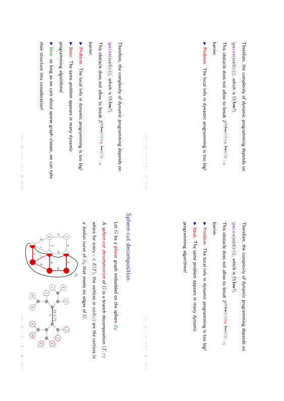
Therefore,

the

complexity

ofdyn

amic

programm

ing

dep

ends

on

|pairs(m

id(e))|,w

hich

isΩ(b

w!).

This

obstacle

does

not

allowto

break2

O(b

w(G

)·log

bw

(G))·

n

barrier.

Prob

lem:

The

local

info

indyn

amic

programm

ing

isto

obig!

Therefore,

the

complexity

ofdyn

amic

programm

ing

dep

ends

on

|pairs(m

id(e))|,w

hich

isΩ(b

w!).

This

obstacle

does

not

allowto

break2

O(b

w(G

)·log

bw

(G))·

n

barrier.

Prob

lem:

The

local

info

indyn

amic

programm

ing

isto

obig!

Issu

e:T

he

same

problem

appears

inm

any

dyn

amic

programm

ing

algorithm

s!

Therefore,

the

complexity

ofdyn

amic

programm

ing

dep

ends

on

|pairs(m

id(e))|,w

hich

isΩ(b

w!).

This

obstacle

does

not

allowto

break2

O(b

w(G

)·log

bw

(G))·

n

barrier.

Prob

lem:

The

local

info

indyn

amic

programm

ing

isto

obig!

Issu

e:T

he

same

problem

appears

inm

any

dyn

amic

programm

ing

algorithm

s!

Id

ea:as

long

aswe

careab

out

sparse

graph

classes,we

cantake

their

structu

rein

tocon

sideration

!

Sphere-cut

decomposition

Let

Gbe

aplan

argrap

hem

bed

ded

onth

esp

hereS

0

Asp

here-cu

tdecom

position

ofG

isa

branch

decom

position

(T,τ)

where

forevery

e∈E(T),

the

verticesinmid(e)

areth

evertices

in

aJord

ancu

rveofS

0th

atm

eetsno

edges

ofG

.

j

l

bm

k g2,5

,7

c

ad

fhi

ec

8

46

13

ab

fg

cd

m

hi

jk

l 5

7

2

Oe

Seym

our-Thom

as1994,

Dorn-P

enninkx-Bodlaender-F

F

2005Theorem

Every

plan

argrap

hG

ofbran

chw

idth

ℓhas

asp

here-cu

t

decom

position

ofw

idth

ℓ.T

his

decom

position

canbe

constru

cted

inO( n

3)step

s.

For

doin

gdyn

amic

programm

ing

ona

sphere

cut

decom

position

(T,τ)

ofw

idth

ℓwe

defi

ne,

forevery

e∈E(T)

the

set

pairs(m

id(e))be

the

setof

allpairin

gsofmid(e)

For

doin

gdyn

amic

programm

ing

ona

sphere

cut

decom

position

(T, τ)

ofw

idth

ℓwe

defi

ne,

forevery

e∈E(T)

the

set

pairs(m

id(e))be

the

setof

allpairin

gsofmid(e)

The

“usu

al”bou

nd

onth

esize

ofpairs(m

id(e))is2

O(ℓ·lo

gℓ)

For

doin

gdyn

amic

programm

ing

ona

sphere

cut

decom

position

(T, τ)

ofw

idth

ℓwe

defi

ne,

forevery

e∈E(T)

the

set

pairs(m

id(e))be

the

setof

allpairin

gsofmid(e)

The

“usu

al”bou

nd

onth

esize

ofpairs(m

id(e))is2

O(ℓ·lo

gℓ)

How

ever,we

now

have

that

1:th

evertices

ofmid(e)

layon

the

bou

ndary

ofa

disk

and

2:th

epairin

gscan

not

be

crossing

becau

seof

plan

arity.

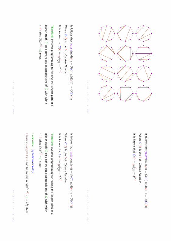
Itfollow

sth

atpairs(m

id(e))=

O(C(|m

id(e)|))=

O(C(ℓ))

Where

C(ℓ)

isth

eℓ-th

Catalan

Num

ber.

Itis

know

nth

atC(ℓ)∼

4ℓ

ℓ3/2 √

π=2

O(ℓ)

Itfollow

sth

atpairs(m

id(e))=

O(C(|m

id(e)|))=

O(C(ℓ))

Where

C(ℓ)

isth

eℓ-th

Catalan

Num

ber.

Itis

know

nth

atC(ℓ)∼

4ℓ

ℓ3/2 √

π=2

O(ℓ)

Therefore:

dyn

amic

programm

ing

forfindin

gth

elon

gestpath

ofa

plan

argrap

hG

ona

sphere

cut

decom

position

sof

Gw

ithw

idth

≤ℓ

takesO(2

O(ℓ)·

n)step

s.

Itfollow

sth

atpairs(m

id(e))=

O(C(|m

id(e)|))=

O(C(ℓ))

Where

C(ℓ)

isth

eℓ-th

Catalan

Num

ber.

Itis

know

nth

atC(ℓ)∼

4ℓ

ℓ3/2 √

π=2

O(ℓ)

Therefore:

dyn

amic

programm

ing

forfindin

gth

elon

gestpath

ofa

plan

argrap

hG

ona

sphere

cut

decom

position

sof

Gw

ithw

idth

≤ℓ

takesO(2

O(ℓ)·

n)step

s.

Con

clusion

:[by

bid

imen

sionality]

Plan

ark-L

ongest

Path

canbe

solvedin

O(2

O( √

k)·

n+

n3)

steps

T

he

same

hold

sfor

severaloth

erprob

lems

where

anan

alogue

of

pairs(m

id(e))can

be

defi

ned

forcon

trolling

the

sizeof

the

tables

in

dyn

amic

programm

ing.

T

he

same

hold

sfor

severaloth

erprob

lems

where

anan

alogue

of

pairs(m

id(e))can

be

defi

ned

forcon

trolling

the

sizeof

the

tables

in

dyn

amic

programm

ing.

Like

that

one

candesign

2O

( √k)· n

O(1

)step

algorithm

sfor

param

eterizedplan

arversion

sof

Cycle

Cover,Path

Cover,

Longest

Cycle,C

onnected

Domin

atin

gSet,Feedback

Vertex

Set,H

amilt

onia

nC

ycle,G

raph

Metric

TSP

,M

ax

Leaf

Tree,etc.

How

touse

Catalan

structurein

non-planargraphs?

We

sayth

atbran

chdecom

position

(T,τ)

ofw

idth

ℓhas

the

Catalan

Stru

cture

fork-L

ongest

Path

if

∀e∈

E(T

)pairs(m

id(e))=2

O(ℓ)

How

touse

Catalan

structurein

non-planargraphs?

We

sayth

atbran

chdecom

position

(T,τ)

ofw

idth

ℓhas

the

Catalan

Stru

cture

fork-L

ongest

Path

if

∀e∈

E(T

)pairs(m

id(e))=2

O(ℓ)

W

ehave

seenth

at,for

plan

argrap

hs,

one

cancon

struct

a

branch

decom

position

with

the

Catalan

structu

refor

the

k-L

ongest

Path

problem

.

Dorn-F

F-T

hilikos2008

Theorem

For

any

H-m

inor

freegrap

hclassG

there

isa

constan

tcH

(dep

endin

gon

lyon

H)

such

that

the

followin

ghold

s:For

every

graph

G∈G

and

any

positive

integer

w,it

ispossib

leto

constru

ct

acH·n

O(1

)-stepalgorith

mth

atou

tputs

either

1.a

correctrep

ortth

atbw(G)

>w

or

2.a

branch

decom

position

(T,τ)

with

the

Catalan

structu

rean

d

ofw

idth

cH·w

.

Consequences:

For

H-m

inor

freegrap

hs,

one

cancon

struct

analgorith

mth

at

solvesth

ek-L

ongest

Path

problem

in2

O( √

k)·

nO

(1)

steps.

Consequences:

For

H-m

inor

freegrap

hs,

one

cancon

struct

analgorith

mth

at

solvesth

ek-L

ongest

Path

problem

in2

O( √

k)·

nO

(1)

steps.

U

sing

the

same

result

one

canalso

solve,for

H-m

inor

free

graphs,

in2

O( √

k)·

nO

(1)

steps,

the

the

standard

param

eterization

ofLongest

Cycle,an

dC

ycle/Path

Cover,param

eterized

either

byth

etotal

length

ofth

ecycles/p

aths

orth

enum

ber

ofth

e

cycles/path

s.

By

applyin

gm

odifi

cations

itis

possib

leto

defi

ne

anan

alogue

of

Catalan

Stru

cture

property

foroth

erprob

lems

likeFeedback

Vertex

Set,C

onnected

Domin

atin

gSet,an

dM

ax

Leaf

Tree

Pro

ofidea:

againG

raphM

inors

[Rob

ertsonan

dSeym

our

–G

M16]:

any

H-m

inor

freegrap

hcan

rough

lybe

obtain

edby

iden

tifying

ina

tree-likeway

small

cliques

ofa

collectionof

compon

ents

that

arealm

ostem

bed

dab

leon

bou

nded

genus

surfaces.

Pro

ofidea:

againG

raphM

inors

[Rob

ertsonan

dSeym

our

–G

M16]:

any

H-m

inor

freegrap

hcan

rough

lybe

obtain

edby

iden

tifying

ina

tree-likeway

small

cliques

ofa

collectionof

compon

ents

that

arealm

ostem

bed

dab

leon

bou

nded

genus

surfaces.

Pro

ofid

ea:W

econ

struct

an“alm

ost”-plan

arizing

with

certain

topological

properties,

able

tored

uce

the

high

genus

“almost”-em

bed

din

gsto

plan

aron

esw

here

the

plan

arizing

vertices

are“alm

ost”-cyclicallyarran

gedin

the

plain

.

Inth

eplan

e,we

use

sphere

cut

decom

position

s,th

atperm

itto

enco

de

collections

ofpath

sth

atm

aypass

throu

gha

separator

asnon

crossing

pairin

gsof

the

verticesof

acycle.

Inth

eplan

e,we

use

sphere

cut

decom

position

s,th

atperm

itto

enco

de

collections

ofpath

sth

atm

aypass

throu

gha

separator

asnon

crossing

pairin

gsof

the

verticesof

acycle.

T

his

provides

the

so-calledCatalan

structu

reof

the

decom

position

and

perm

itsus

tosu

itably

bou

nd

the

ways

apath

may

crossits

separators.

Inth

eplan

e,we

use

sphere

cut

decom

position

s,th

atperm

itto

enco

de

collections

ofpath

sth

atm

aypass

throu

gha

separator

asnon

crossing

pairin

gsof

the

verticesof

acycle.

T

his

provides

the

so-calledCatalan

structu

reof

the

decom

position

and

perm

itsus

tosu

itably

bou

nd

the

ways

apath

may

crossits

separators.

T

his

decom

position

isused

tobuild

adecom

position

onth

ein

itial

almost

embed

dib

legrap

h(follow

ing

the

tree-likeway

these

compon

ents

arelin

kedtogeth

er).

Open

problems

I

Low

erbou

nds

ondyn

amic

programm

ing

overbran

chw

idth

.Is

it

possib

leto

prove(u

pto

some

conjectu

rein

complexity

theory)

that

Lon

gestPath

ongrap

hs

ofbran

chw

idth

ℓcan

not

be

solvedin

2o(ℓ

log

ℓ)m?

Open

problems

I

Low

erbou

nds

ondyn

amic

programm

ing

overbran

chw

idth

.Is

it

possib

leto

prove(u

pto

some

conjectu

rein

complexity

theory)

that

Lon

gestPath

ongrap

hs

ofbran

chw

idth

ℓcan

not

be

solvedin

2o(ℓ

log

ℓ)m?

Can

Vertex

Cover

be

solvedfaster

than

2ℓn

O(1

)?

Open

problems

II

When

applyin

gou

rtech

niq

ue

ondiff

erent

problem

swe

defi

ne,

for

eachon

eof

them

,an

appropriate

analogu

eof

pairs

and

prove

that

italso

satisfies

the

Catalan

structu

reprop

erty(i.e.

isbou

nded

by2

O(|m

id(e)|)).

Open

problems

II

When

applyin

gou

rtech

niq

ue

ondiff

erent

problem

swe

defi

ne,

for

eachon

eof

them

,an

appropriate

analogu

eof

pairs

and

prove

that

italso

satisfies

the

Catalan

structu

reprop

erty(i.e.

isbou

nded

by2

O(|m

id(e)|)).

It

isch

allengin

gto

find

aclassifi

cationcriterion

(logicalor

combin

atorial)for

the

problem

sth

atare

amen

able

toth

is

approach

.

Open

problems

III

Suffi

cient

condition

:B

idim

ension

ality(p

lus

fastdyn

amic

programm

ing)

yields

subexp

onen

tialparam

eterizedalgorith

m.

Open

problems

III

Suffi

cient

condition

:B

idim

ension

ality(p

lus

fastdyn

amic

programm

ing)

yields

subexp

onen

tialparam

eterizedalgorith

m.

What

areth

enecessary

condition

s?

Rem

ark:Every

problem

onplan

argrap

hs

forw

hich

we

know

subexp

onen

tialparam

eterizedalgorith

mis

either

bid

imen

sional,

or

canbe

reduced

toa

bid

imen

sional

problem

.

Open

problems

IV

Bran

chw

idth

:Polyn

omial

time

algorithm

forgrap

hs

ofbou

nded

genus?

H-m

inor

freegrap

hs?

Further

reading.Sub

exponential

algorithms

and

bidimensionality

J.A

lber,H

.L.B

odlaender,H

.Fernau,T

.K

loks,

and

R.N

iedermeie

r,Fixed

param

eteralgorith

ms

for

dom

inatin

gset

and

relatedprob

lems

onplan

argrap

hs,

Algorith

mica,

33(2002),

pp.461–493.

E.D

.D

emain

e,F.V

.Fomin

,M

.H

ajia

ghayi,

and

D.M

.T

hil

ikos,

Subexp

onen

tialparam

eterizedalgorith

ms

ongrap

hs

ofbou

nded

genus

and

H-m

inor-free

graphs,

Journ

al

ofth

eACM

,52

(2005),pp.866–893.

Further

reading.Catalan

structuresand

dynamic

programm

ing

F.D

orn,E.Pennin

kx,H

.B

odlaender,and

F.V

.

Fomin

,Effi

cient

exactalgorith

ms

onplan

argrap

hs:

Exp

loiting

sphere

cut

branch

decom

position

s,Pro

ceedin

gsof

the

13th

Annual

Europ

eanSym

posiu

mon

Algorith

ms

(ESA

2005),

vol.3669

ofLN

CS,Sprin

ger,2005,

pp.95–106.

F.D

orn,F.V

.Fomin

,and

D.M

.T

hil

ikos,

Catalan

structu

resan

ddyn

amic

programm

ing

onH

-min

or-freegrap

hs,

inPro

ceedin

gsof

the

19thA

nnual

ACM

-SIA

MSym

posiu

mon

Discrete

Algorith

ms

(SO

DA

2008),ACM

-SIA

M,pp.631–640.

Further

reading.Surveys

E.D

emain

eand

M.H

ajia

ghayi,

The

bid

imen

sionality

theory

and

itsalgorith

mic

application

s,T

he

Com

puter

Journ

al,

(2007),pp.332–337.

F.D

orn,F.V

.Fomin

,and

D.M

.T

hil

ikos,

Subexp

onen

tialparam

eterizedalgorith

ms,

Com

puter

Scien

ce

Review

,2

(2008),pp.29–39.

Fabrizio Grandoni

A Measure & ConquerApproach for the Analysis of

Exact Algorithms

A Measure & Conquer Approach for theAnalysis of Exact Algorithms

Fabrizio Grandoni∗

May 19, 2009

1 Introduction

The aim of exact algorithms is to exactly solve NP-hard problems in the smallest possible(exponential) worst-case running time. This field dates back to the sixties and seventies,and it has started to attract a growing interest in the last two decades. There are severalexplanations to the increasing interest in exact algorithms:

• There are certain applications that require exact solutions of NP-hard problems, al-though this might only be possible for moderate input sizes. This holds in particularfor NP-complete decision problems.

• Approximation algorithms are not always satisfactory. Various problems are hard toapproximate. For example, maximum independent set is hard to approximate withinO(n1−ε), for any constant ε > 0, unless P = NP [25].

• A reduction of the base of the exponential running time, say from O(2n) to O(1.9n),increases the size of the instances solvable within a given amount of time by a constantmultiplicative factor; running a given exponential algorithm on a faster computer canenlarge the mentioned size only by a (small) additive factor.

• The design and analysis of exact algorithms leads to a better understanding of NP-hardproblems and initiates interesting new combinatorial and algorithmic challenges.

1.1 Branch & Reduce algorithms

One of the major techniques in the design of exact algorithms is Branch & Reduce, whichtraces back to the paper of Davis and Putnam [5] (see also [4]). A typical Branch & Reducealgorithm for a given problem P works as follows. If P is a base instance, the problems is solveddirectly in polynomial time. Otherwise the algorithm transforms the problem by applying aset of polynomial-time reduction rules. Then it branches, in polynomial-time, on two or moresubproblems P1, . . . ,Ph, according to a proper set of branching rules. Such subproblems aresolved recursively, and the partial solutions obtained are eventually combined, in polynomialtime, to get a solution for P.

∗Dipartimento di Informatica, Sistemi e Produzione, Universita di Roma Tor Vergata, via del Politecnico1, 00133 Roma, Italy, grandoni@disp.uniroma2.it.

1

Branch & Reduce algorithms are usually analyzed with the bounded search tree technique.Suppose we wish to find a time bound for a problem of size n. Assume that the depth of thesearch tree is polynomially bounded (which is trivially true in most cases). It is sufficient tobound the maximum number P (n) of base instances generated by the algorithm: the runningtime will be O∗(P (n))1. If P is a base instance, trivially P (n) = 1. Otherwise, consider apossible branching step b, generating subproblems Pb

1, . . . ,Pbh(b), and let n − δb

j < n be thesize of subproblem Pb

j . The vector δb = (δb1, . . . , δ

bh(b)) is sometimes called branching vector.

It follows that

P (n) ≤h(b)∑j=1

P (n− δbj).

Consider function

f b(x) = 1−h(b)∑j=1

x−δbj .

This function has a unique positive root λb = bf(δb) (branching factor of δb). Branchingfactors can be easily computed numerically (see Appendix A). It turns out that P (n) ≤ λn,where λ = maxbλb.

We say that a branching vector δ dominates a branching vector δ′ if δ ≤ δ′, i.e. δ iscomponent-wise not larger than δ′. It is not hard to see that, when δ ≤ δ′, bf(δ) ≥ bf(δ′).Hence, with respect to the running time analysis, it is sufficient to consider a dominating setof branching vectors. In other words, each time we replace the branching vector of a feasiblebranching with a branching vector dominating it, we obtain a pessimistic estimate of therunning time. These properties will be extensively used in these notes.

1.2 Measure & Conquer

Branch & Reduce algorithms have been used for more than 40 years to solve NP-hard prob-lems. The fastest known such algorithms are often very complicated. Typically, they consistof a long list of non-trivial branching and reduction rules, and are designed by means of along and tedious case distinction. Despite that, the analytical tools available are still far fromproducing tight worst-case running time bounds for this kind of algorithms.

In these notes we present an improved analytical tool, that we called Measure & Conquer.In the standard analysis, n is both the measure used in the analysis and the quantity interms of which the final time bound is expressed. However, one is free to use any, possiblysophisticated, measure m in the analysis, provided that m ≤ f(n) for some known functionf . This way, one achieves a time bound of the kind O∗(λm) = O∗(λf(n)), which is in thedesired form. The idea behind Measure & Conquer is focusing on the choice of the measure.In fact, a more sophisticated measure may capture phenomena which standard measures arenot able to exploit, and hence lead to a tighter analysis of a given algorithm.

We apply Measure & Conquer to a toy algorithm mis for MIS. According to a standardanalysis, the running time of this algorithm is O∗(1.33n). Thanks to a better measure, weprove that the same algorithm has indeed running time O∗(1.26n). This result shows thata good choice of the measure can have a tremendous impact on the time bounds achievable,

1Throughout this paper we use a modified big-Oh notation that suppresses all polynomially bounded factors.For functions f and g we write f(n) = O∗(g(n)) if f(n) = O(g(n)poly(n)), where poly(n) is a polynomial.Also while speaking about graph problems, we use n to denote the number of nodes in the graph.

2

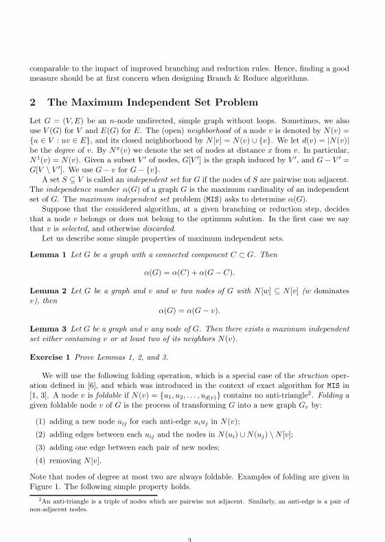
comparable to the impact of improved branching and reduction rules. Hence, finding a goodmeasure should be at first concern when designing Branch & Reduce algorithms.

2 The Maximum Independent Set Problem

Let G = (V,E) be an n-node undirected, simple graph without loops. Sometimes, we alsouse V (G) for V and E(G) for E. The (open) neighborhood of a node v is denoted by N(v) =u ∈ V : uv ∈ E, and its closed neighborhood by N [v] = N(v) ∪ v. We let d(v) = |N(v)|be the degree of v. By Nx(v) we denote the set of nodes at distance x from v. In particular,N1(v) = N(v). Given a subset V ′ of nodes, G[V ′] is the graph induced by V ′, and G− V ′ =G[V \ V ′]. We use G− v for G− v.

A set S ⊆ V is called an independent set for G if the nodes of S are pairwise non adjacent.The independence number α(G) of a graph G is the maximum cardinality of an independentset of G. The maximum independent set problem (MIS) asks to determine α(G).

Suppose that the considered algorithm, at a given branching or reduction step, decidesthat a node v belongs or does not belong to the optimum solution. In the first case we saythat v is selected, and otherwise discarded.

Let us describe some simple properties of maximum independent sets.

Lemma 1 Let G be a graph with a connected component C ⊂ G. Then

α(G) = α(C) + α(G − C).

Lemma 2 Let G be a graph and v and w two nodes of G with N [w] ⊆ N [v] (w dominatesv), then

α(G) = α(G − v).

Lemma 3 Let G be a graph and v any node of G. Then there exists a maximum independentset either containing v or at least two of its neighbors N(v).

Exercise 1 Prove Lemmas 1, 2, and 3.

We will use the following folding operation, which is a special case of the struction oper-ation defined in [6], and which was introduced in the context of exact algorithm for MIS in[1, 3]. A node v is foldable if N(v) = u1, u2, . . . , ud(v) contains no anti-triangle2. Folding agiven foldable node v of G is the process of transforming G into a new graph Gv by:

(1) adding a new node uij for each anti-edge uiuj in N(v);

(2) adding edges between each uij and the nodes in N(ui) ∪N(uj) \N [v];

(3) adding one edge between each pair of new nodes;

(4) removing N [v].

Note that nodes of degree at most two are always foldable. Examples of folding are given inFigure 1. The following simple property holds.

2An anti-triangle is a triple of nodes which are pairwise not adjacent. Similarly, an anti-edge is a pair ofnon-adjacent nodes.

3

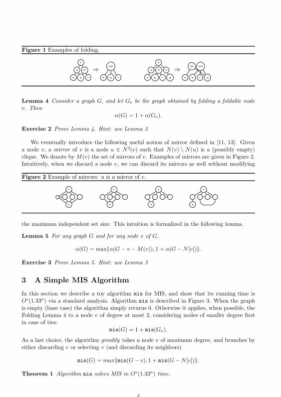
Figure 1 Examples of folding.

v

u w

a b c

⇒ uw

a b c

v

u w z

a b c d

⇒ uz wz

a b c d

Lemma 4 Consider a graph G, and let Gv be the graph obtained by folding a foldable nodev. Then

α(G) = 1 + α(Gv).

Exercise 2 Prove Lemma 4. Hint: use Lemma 3

We eventually introduce the following useful notion of mirror defined in [11, 13]. Givena node v, a mirror of v is a node u ∈ N2(v) such that N(v) \ N(u) is a (possibly empty)clique. We denote by M(v) the set of mirrors of v. Examples of mirrors are given in Figure 2.Intuitively, when we discard a node v, we can discard its mirrors as well without modifying

Figure 2 Example of mirrors: u is a mirror of v.

v

u

v

u

v

u

v

u

the maximum independent set size. This intuition is formalized in the following lemma.

Lemma 5 For any graph G and for any node v of G,

α(G) = maxα(G − v −M(v)), 1 + α(G−N [v]).

Exercise 3 Prove Lemma 5. Hint: use Lemma 3

3 A Simple MIS Algorithm

In this section we describe a toy algorithm mis for MIS, and show that its running time isO∗(1.33n) via a standard analysis. Algorithm mis is described in Figure 3. When the graphis empty (base case) the algorithm simply returns 0. Otherwise it applies, when possible, theFolding Lemma 4 to a node v of degree at most 2, considering nodes of smaller degree firstin case of ties:

mis(G) = 1 + mis(Gv).

As a last choice, the algorithm greedily takes a node v of maximum degree, and branches byeither discarding v or selecting v (and discarding its neighbors)

mis(G) = maxmis(G− v), 1 + mis(G−N [v]).

Theorem 1 Algorithm mis solves MIS in O∗(1.33n) time.

4

Figure 3 Algorithm mis for the maximum independent set problem.

int mis(G) if (G = ∅) return 0; //Base case//FoldingTake v of minimum degreeif (d(v) ≤ 2) return 1 + mis(Gv);//“Greedy” branchingTake v of maximum degree;return max mis(G− v), 1 + mis(G−N [v]) ;

Proof. Let P (n) be the number of base instances generated by the algorithm to solvean instance of size n. The depth of the recursion is O(n) since in each step the number ofnodes decreases at least by one. Moreover, the algorithm takes polynomial time, excludingthe time needed for the recursive calls. It follows that the running time of the algorithm isO(P (n)nO(1)) = O∗(P (n)).

We next show by induction that P (n) ≤ λn for λ < 1.33. In the base case n = 0 andP (0) = 1 ≤ λ0 for every λ > 0. When the algorithm folds a node, the number of nodesdecreases at least by one. Hence, for every λ ≥ 1,

P (n) ≤ P (n− 1) ≤ λn−1 ≤ λn.

When the algorithm branches at a node v with d(v) ≥ 4, in one subproblem it removes 1node (i.e. v), and in the other it removes 1 + d(v) ≥ 5 nodes (i.e. N [v]). Let λ1 = bf(1, 5) =1.32 . . . < 1.33 be the positive root of 1− x−1 − x−5. For λ ≥ λ1 we obtain

P (n) ≤ P (n− 1) + P (n− 5) ≤ λn−1 + λn−5 ≤ λn.

Otherwise, the algorithm branches at a node v of degree exactly 3, hence removing either1 or 4 nodes. However, in the first case a node of degree 2 is folded afterwards, with theremoval of at least 2 more nodes. Let λ2 = bf(3, 4) = 1.22 . . . < 1.23 be the positive root of1− x−3 − x−4. For λ ≥ λ2,

P (n) ≤ P (n− 3) + P (n− 4) ≤ λn−3 + λn−4 ≤ λn.

The claim follows. The time bound above is the best one can achieve via a standard analysis. We will see howa non-standard analysis can provide much better time bounds.

4 A Refined Analysis via Measure & Conquer

The classical approach to improve on mis would be designing refined branching and reductionrules. In particular, one tries to improve on the tight recurrences. We next show how to geta much better time bound thanks to a better measure of subproblems size (without changing

5

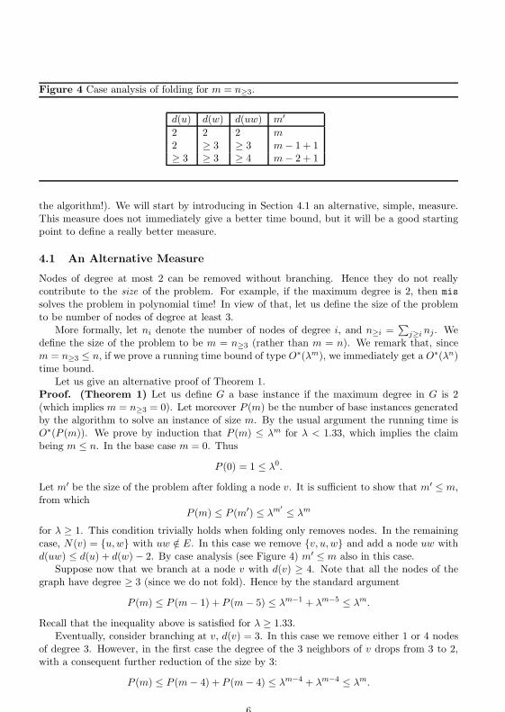
Figure 4 Case analysis of folding for m = n≥3.

d(u) d(w) d(uw) m′

2 2 2 m2 ≥ 3 ≥ 3 m− 1 + 1≥ 3 ≥ 3 ≥ 4 m− 2 + 1

the algorithm!). We will start by introducing in Section 4.1 an alternative, simple, measure.This measure does not immediately give a better time bound, but it will be a good startingpoint to define a really better measure.

4.1 An Alternative Measure

Nodes of degree at most 2 can be removed without branching. Hence they do not reallycontribute to the size of the problem. For example, if the maximum degree is 2, then missolves the problem in polynomial time! In view of that, let us define the size of the problemto be number of nodes of degree at least 3.

More formally, let ni denote the number of nodes of degree i, and n≥i =∑

j≥i nj. Wedefine the size of the problem to be m = n≥3 (rather than m = n). We remark that, sincem = n≥3 ≤ n, if we prove a running time bound of type O∗(λm), we immediately get a O∗(λn)time bound.

Let us give an alternative proof of Theorem 1.Proof. (Theorem 1) Let us define G a base instance if the maximum degree in G is 2(which implies m = n≥3 = 0). Let moreover P (m) be the number of base instances generatedby the algorithm to solve an instance of size m. By the usual argument the running time isO∗(P (m)). We prove by induction that P (m) ≤ λm for λ < 1.33, which implies the claimbeing m ≤ n. In the base case m = 0. Thus

P (0) = 1 ≤ λ0.

Let m′ be the size of the problem after folding a node v. It is sufficient to show that m′ ≤ m,from which

P (m) ≤ P (m′) ≤ λm′ ≤ λm

for λ ≥ 1. This condition trivially holds when folding only removes nodes. In the remainingcase, N(v) = u,w with uw /∈ E. In this case we remove v, u,w and add a node uw withd(uw) ≤ d(u) + d(w) − 2. By case analysis (see Figure 4) m′ ≤ m also in this case.

Suppose now that we branch at a node v with d(v) ≥ 4. Note that all the nodes of thegraph have degree ≥ 3 (since we do not fold). Hence by the standard argument

P (m) ≤ P (m− 1) + P (m− 5) ≤ λm−1 + λm−5 ≤ λm.

Recall that the inequality above is satisfied for λ ≥ 1.33.Eventually, consider branching at v, d(v) = 3. In this case we remove either 1 or 4 nodes

of degree 3. However, in the first case the degree of the 3 neighbors of v drops from 3 to 2,with a consequent further reduction of the size by 3:

P (m) ≤ P (m− 4) + P (m− 4) ≤ λm−4 + λm−4 ≤ λm.

6

The inequality above is satisfied for λ ≥ bf(4, 4) = 1.18 . . .. The claim follows.

4.2 A Better Measure

When we branch at a node of large degree, we decrement by 1 the degree of many othernodes. This is beneficial on long term, since we can remove nodes of degree at most 2 withoutbranching. We are not exploiting this fact to its full extent in the current analysis.

An idea is then to attribute a larger weight ωi ≤ 1 to nodes v of larger degree i, andlet the size of the problem be the sum of node sizes. This way, when the degree of a nodedecreases, the size of the problem decreases as well. More formally, for a constant ω ∈ (0, 1]to be fixed later, we let

ωi =

0 if i ≤ 2;ω if i = 3;1 otherwise.

We also use ω(v) for ωd(v). The size m = m(G) of graph G = (V,E) is

m =∑v∈V

w(v) = ω · n3 + n≥4.

Thanks to this new measure of subproblems size, we are able to refine the analysis of mis.

Theorem 2 Algorithm mis solves MIS in O∗(1.29n) time.

Proof. With the usual notation, let us show that P (m) ≤ λm for λ < 1.29. In the basecase m = 0, and thus

P (0) = 1 ≤ λ0.

In case of folding of node v, let m′ = m(Gv) be the size of the corresponding subproblem.Also in this case it is sufficient to show that m′ ≤ m. This condition is satisfied when nodesare only removed (being the weight increasing with the degree). The unique remaining caseis N(v) = u,w, with u and w not adjacent. In this case we remove v, u,w, and add anode uw with d(uw) ≤ d(u) + d(w)− 2. Hence it is sufficient to show that

ω(v) + ω(u) + ω(w)− ω(uw) = ω(u) + ω(w) − ω(uw) ≥ 0.

By a simple case analysis (see Figure 5), it follows that this condition holds for ω ≥ 0.5.Consider now the case of branching at a node v, d(v) ≥ 5. Let di be the degree of the ith

neighbor of v (which thus has weight ωdi). Then

P (m) ≤ P (m− ωd(v) −d(v)∑i=1

(ωdi− ωdi−1)) + P (m− ωd(v) −

d(v)∑i=1

ωdi)

≤ P (m− 1−5∑

i=1

(ωdi− ωdi−1)) + P (s− 1−

5∑i=1

ωdi).

Observe that we can replace di ≥ 6 with di = 5. In fact in both cases ωdi= 1 and ωdi

−ωdi−1 =0. Hence we can assume di ∈ 3, 4, 5. This is crucial to obtain a finite number of recurrences!We obtain the following set of recurrences

P (m) ≤ P (m− 1− t3(ω − 0)− t4(1− ω)− t5(1− 1)) + P (m− 1− t3 ω − t4 − t5),

7

Figure 5 Case analysis of folding for m = ωn3 + n≥4.

d(u) d(w) d(uw) ω(u) + ω(w)− ω(uw) ≥ 02 2 2 0 + 0− 0 ≥ 02 3 3 0 + ω − ω ≥ 02 ≥ 4 ≥ 4 0 + 1− 1 ≥ 03 3 4 ω + ω − 1 ≥ 03 ≥ 4 ≥ 4 ω + 1− 1 ≥ 0≥ 4 ≥ 4 ≥ 4 1 + 1− 1 ≥ 0

where t3, t4, and t5 are non-negative integers satisfying t3 + t4 + t5 = 5. (Intuitively, ti is thenumber of neighbors of v of degree i).

Consider now branching at a node v, d(v) = 4. By a similar argument (with di ∈ 3, 4),we obtain

P (m) ≤

P (m− 1− 4 · ω − 0 · (1− ω)) + P (m− 1− 4 · ω − 0 · 1)P (m− 1− 3 · ω − 1 · (1− ω)) + P (m− 1− 3 · ω − 1 · 1)P (m− 1− 2 · ω − 2 · (1− ω)) + P (m− 1− 2 · ω − 2 · 1)P (m− 1− 1 · ω − 3 · (1− ω)) + P (m− 1− 1 · ω − 3 · 1)P (m− 1− 0 · ω − 4 · (1− ω)) + P (m− 1− 0 · ω − 4 · 1)

Consider eventually branching at a node v, d(v) = 3. By an analogous argument (withω(v) = ω3 = ω and di = 3)

P (m) ≤ P (m− ω − 3ω) + P (m− ω − 3ω).

For every ω ∈ [1/2, 1], the set of recurrences above provides an upper bound λ(ω) onλ. Our goal is minimizing λ(ω) (hence getting a better time bound). Via exhaustive searchover a grid of values for ω we obtained λ(0.7) < 1.29 (see Appendix B for a C++ programcomputing it). The claim follows.

4.3 An Even Better Measure

We can extend the analysis from previous section to larger degrees. For example, we mightlet the weight ωi associated to degree-i nodes be:

ωi =

0 if i ≤ 2;ω if i = 3;ω′ if i = 4;1 otherwise.

Here ω and ω′ are two proper constants, with 0 < ω ≤ ω′ ≤ 1. Using this measure, and ananalysis similar to the one from previous section, it is not hard to prove the following result(see Appendix C for a C++ program optimizing the weights).

8

Theorem 3 Algorithm mis solves MIS in O∗(1.26n) time.

Exercise 4 Prove the theorem above. Hint: ω = 0.750 and ω′ = 0.951.

Exercise 5 What happens if we set ω5 = ω′′ for a further weight ω′ ≤ ω′′ ≤ 1? Do you seeany pattern?

Exercise 6 Design a better algorithm for MIS, possibly using the other mentioned reduc-tion rules (mirroring etc.). Analyze this algorithm in the standard way and via Measure &Conquer.

Exercise 7 Can you see an alternative, promising measure for MIS?

5 Lower bounds

Despite the big improvements in the running time bounds, it might be that our refined analysisis still far from being tight. Hence, it is natural to ask for (exponential) lower bounds. Noticethat we are concerned with lower bounds on the complexity of a particular algorithm, andnot with lower bounds on the complexity of an algorithmic problem. A lower bound may givean idea of how far the analysis is from being tight.

In this section we prove a Ω(2n/4) lower bound on the running time of mis. The largegap between the upper and lower bound for mis suggests the possibility that the analysis ofthat algorithm can be further refined (possibly by measuring the size of the subproblems ina further refined way).

Theorem 4 The running time of mis is Ω(2n/4) = Ω(1.18n).

Proof. Consider the graph Gk consisting of k = n/4 copies of a 4-clique (see Figure 6).We let P (k) be the number of subproblems generated by mis to solve MIS on Gk. Considerany clique C = a, b, c, d ∈ Gk. The algorithm might branch at a. In the subproblem wherea is discarded, the algorithm removes b, c, and d via folding. In the other subproblem thealgorithm removes N [a] = a, b, c, d. Hence in both cases C is deleted from the graph, leavingan instance Gk−1 which is solved recursively. We thus obtain the following recurrences:

P (k) ≥

2P (k − 1) if k ≥ 1;1 if k = 0.

We can conclude that P (k) ≥ 2k = 2n/4.

Exercise 8 Find a larger lower bound on the running time of mis. Hint: Ω(3n/6) = Ω(1.20n),maybe better.

Exercise 9 Consider the variant of mis where the algorithm, after the base case, brancheson connected components when possible. Can you find a good lower bound on the runningtime of this modified algorithm?

Remark 1 Typically finding lower bounds on connected graphs is much more complicated.

9

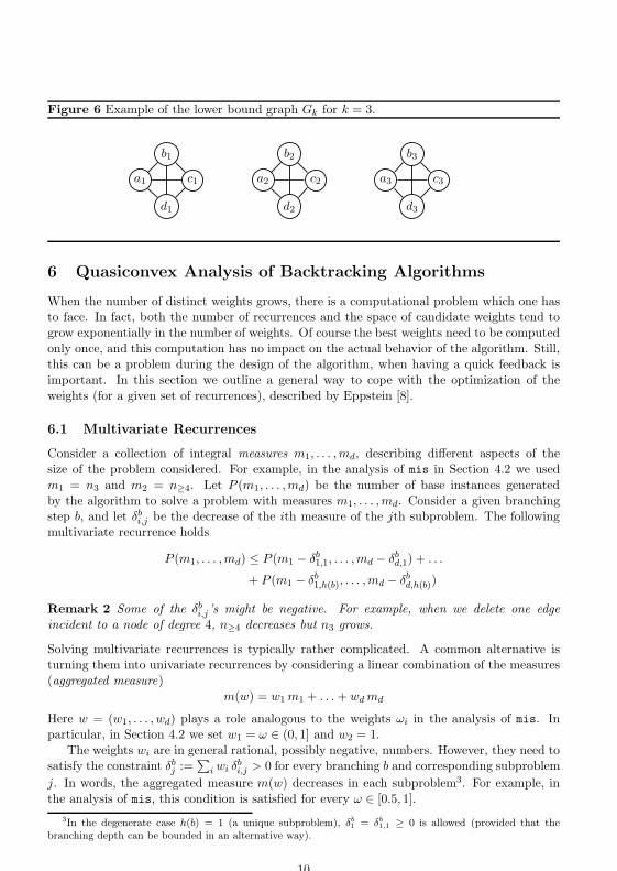
Figure 6 Example of the lower bound graph Gk for k = 3.

a1

b1

c1

d1

a2

b2

c2

d2

a3

b3

c3

d3

6 Quasiconvex Analysis of Backtracking Algorithms

When the number of distinct weights grows, there is a computational problem which one hasto face. In fact, both the number of recurrences and the space of candidate weights tend togrow exponentially in the number of weights. Of course the best weights need to be computedonly once, and this computation has no impact on the actual behavior of the algorithm. Still,this can be a problem during the design of the algorithm, when having a quick feedback isimportant. In this section we outline a general way to cope with the optimization of theweights (for a given set of recurrences), described by Eppstein [8].

6.1 Multivariate Recurrences

Consider a collection of integral measures m1, . . . ,md, describing different aspects of thesize of the problem considered. For example, in the analysis of mis in Section 4.2 we usedm1 = n3 and m2 = n≥4. Let P (m1, . . . ,md) be the number of base instances generatedby the algorithm to solve a problem with measures m1, . . . ,md. Consider a given branchingstep b, and let δb

i,j be the decrease of the ith measure of the jth subproblem. The followingmultivariate recurrence holds

P (m1, . . . ,md) ≤ P (m1 − δb1,1, . . . ,md − δb

d,1) + . . .

+ P (m1 − δb1,h(b), . . . ,md − δb

d,h(b))

Remark 2 Some of the δbi,j ’s might be negative. For example, when we delete one edge

incident to a node of degree 4, n≥4 decreases but n3 grows.

Solving multivariate recurrences is typically rather complicated. A common alternative isturning them into univariate recurrences by considering a linear combination of the measures(aggregated measure)

m(w) = w1 m1 + . . . + wd md

Here w = (w1, . . . , wd) plays a role analogous to the weights ωi in the analysis of mis. Inparticular, in Section 4.2 we set w1 = ω ∈ (0, 1] and w2 = 1.

The weights wi are in general rational, possibly negative, numbers. However, they need tosatisfy the constraint δb

j :=∑

i wi δbi,j > 0 for every branching b and corresponding subproblem

j. In words, the aggregated measure m(w) decreases in each subproblem3. For example, inthe analysis of mis, this condition is satisfied for every ω ∈ [0.5, 1].

3In the degenerate case h(b) = 1 (a unique subproblem), δb1 = δb

1,1 ≥ 0 is allowed (provided that thebranching depth can be bounded in an alternative way).

10

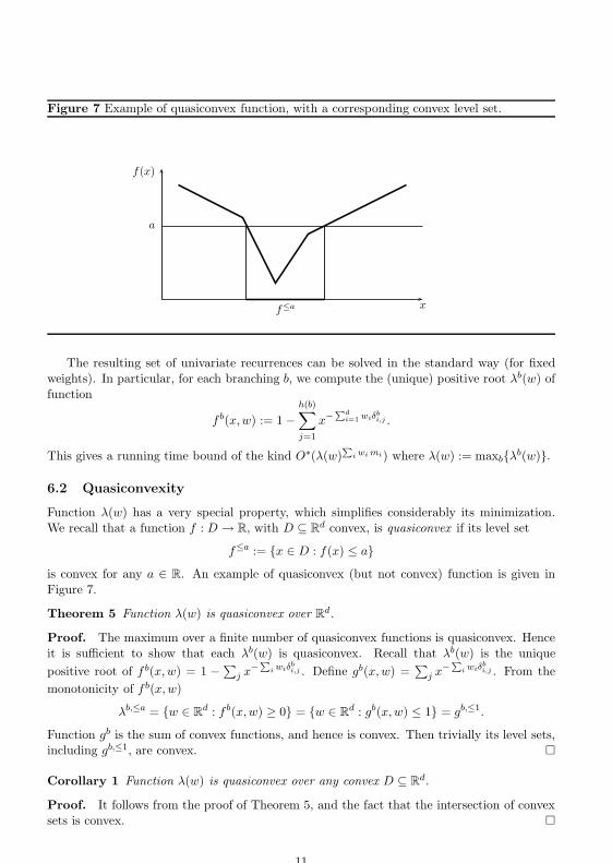
Figure 7 Example of quasiconvex function, with a corresponding convex level set.

f(x)

x

a

f≤a

The resulting set of univariate recurrences can be solved in the standard way (for fixedweights). In particular, for each branching b, we compute the (unique) positive root λb(w) offunction

f b(x,w) := 1−h(b)∑j=1

x−Pd

i=1 wiδbi,j .

This gives a running time bound of the kind O∗(λ(w)P

i wi mi) where λ(w) := maxbλb(w).

6.2 Quasiconvexity

Function λ(w) has a very special property, which simplifies considerably its minimization.We recall that a function f : D → R, with D ⊆ Rd convex, is quasiconvex if its level set

f≤a := x ∈ D : f(x) ≤ ais convex for any a ∈ R. An example of quasiconvex (but not convex) function is given inFigure 7.

Theorem 5 Function λ(w) is quasiconvex over Rd.

Proof. The maximum over a finite number of quasiconvex functions is quasiconvex. Henceit is sufficient to show that each λb(w) is quasiconvex. Recall that λb(w) is the uniquepositive root of f b(x,w) = 1 − ∑

j x−P

i wiδbi,j . Define gb(x,w) =

∑j x−

Pi wiδ

bi,j . From the

monotonicity of f b(x,w)

λb,≤a = w ∈ Rd : f b(x,w) ≥ 0 = w ∈ Rd : gb(x,w) ≤ 1 = gb,≤1.

Function gb is the sum of convex functions, and hence is convex. Then trivially its level sets,including gb,≤1, are convex.

Corollary 1 Function λ(w) is quasiconvex over any convex D ⊆ Rd.

Proof. It follows from the proof of Theorem 5, and the fact that the intersection of convexsets is convex.

11

6.3 Applications to Measure & Conquer

We can use Theorem 5 to optimize the weights in a much faster way with respect to exhaustivegrid search. Suppose we define a set of linear constraints on the weights such that:

(a) the size of each subproblem does not increase;

(b) m(w) ≤ n, where n is a standard measure for the problem.

This gives a convex domain of weights w. On that domain we can compute the minimumvalue λ(w) of the quasiconvex function λ(w). The resulting running time is O∗(λ(w)n).

There are known techniques to find efficiently the minimum of a quasi-convex function (seee.g. [8]). We successfully applied [12, 13, 14] the following, very fast and easy to implement,approach based on randomized local search (in simulated annealing style):

• We start from any feasible initial value w;

• We add to w a random vector ∆ w in a given range [−∆,∆]d;

• If the resulting w′ is feasible and gives λ(w′) ≤ λ(w), we set w = w′;

• We iterate the process, reducing the value of ∆ if no improvement is achieved for a largenumber of steps;

• The process halts when ∆ drops below a given value ∆′.

Appendix D contains a C++ program applying this method to the optimization of the weightsin the analysis of Section 4.3.

Remark 3 The local search algorithm above does not guarantee closeness to the optimalλ(w). However it is accurate in practice. More important, it always provides feasible upperbounds on the running time.

7 Other Examples of Measure & Conquer

In this section we briefly describe other (more or less explicit) applications of the Measure &Conquer approach.

The first non-trivial algorithm for the minimum dominating set problem (MDS) is basedon Measure & Conquer [17, 18]4. The basic idea is developing an algorithm for the minimumset cover problem (MSC). This algorithm is analyzed by measuring the size of the subproblemsin terms of the sum of the number n of sets and number m of elements. The resulting runningtime is O∗(1.381n+m). The size of the MSC formulation of a MDS instance on n nodes is 2n.It follows that MDS can be solved in O∗(1.3812n) = O∗(1.803n) time. The same algorithmis re-analyzed in [10, 13], using a refined measure which assigns different weights to sets ofdifferent size and elements of different frequency. This way the time bound is refined toO∗(1.527n), an impressive improvement.

A similar, but more complex measure is used in [12] to develop the first better-than-trivialalgorithm for the connected version of MDS, where the dominating set is required to induce aconnected graph. Here, besides cardinalities and frequencies, the measure takes into accountthe local connectivity properties of the original graph.

4In the same year, slower but better-than-trivial algorithms for MDS were independently developed in[15, 22].

12

In a paper on 3-coloring and related problems [2], Beigel and Eppstein consider a reductionto constraint satisfaction, and measure the size of the constraint satisfaction problem witha linear combination of the number of variables with three and four values in their domain,respectively. A more sophisticated measure is introduced by Eppstein in the context of cubic-TSP [7]: let F be a given set of forced edges, that is edges that we assume belonging to theoptimum solution. For an input cubic graph G = (V,E), the author measures the size ofthe problem in terms of |V | − |F | − |C|, where C is the set of 4-cycles which form connectedcomponents of G− F .

Gupta et al. [19] used Measure & Conquer while analyzing exact algorithms for findingmaximal induced subgraphs of fixed node degree. Razgon [23], using a non-standard measure,derived the first non-trivial algorithm breaking the O∗(2n) barrier for the feedback vertex setproblem (see also [9]). Kowalik [20] used Measure & Conquer in his branching algorithm forthe edge coloring problem. The analysis of Gasper-Liedloff’s algorithm for the independentdominating set problem in [16] is based on Measure & Conquer. Another example is thepaper by Kratsch and Liedloff on the minimum dominating clique problem [21]. We are alsoaware of a number of other (still unpublished) papers using the same kind of approach.

Measure & Conquer can be used also as a tool to prove tighter combinatorial bounds.For example, using this kind of approach and the same measure which is mentioned abovefor MDS, Fomin et al. [14] proved that the number of minimal dominating sets in a graphis O∗(1.721n). Based on this result, they also derived the first non-trivial exact algorithmsfor the domatic number problem and for the minimum-weight dominating set problem. Thebounds on the number of minimal feedback vertex sets (or maximal induced forests) obtainedin [9] are also based on Measure & Conquer.

Of course, a non-standard measure can be used to design better algorithms in the standardway: one considers the tight recurrences for a given algorithm (and measure), and tries todesign better branching and reduction rules for the corresponding cases. A very recent workby van Rooij and Bodlaender goes in this direction [24].

References

[1] R. Beigel. Finding maximum independent sets in sparse and general graphs. In ACM-SIAM Symposium on Discrete Algorithms (SODA), pages 856–857, 1999.

[2] R. Beigel and D. Eppstein. 3-coloring in time O(1.3289n). Journal of Algorithms,54(2):168–204, 2005.

[3] J. Chen, I. Kanj, and W. Jia. Vertex cover: further observations and further improve-ments. Journal of Algorithms, 41:280–301, 2001.

[4] M. Davis, G. Logemann, and D. Loveland. A machine program for theorem-proving.Communications of the Association for Computing Machinery, 5:394–397, 1962.

[5] M. Davis and H. Putnam. A computing procedure for quantification theory. Journal ofthe Association for Computing Machinery, 7:201–215, 1960.

[6] C. Ebenegger, P. L. Hammer, and D. de Werra. Pseudo-boolean functions and stabilityof graphs. Annals of Discrete Mathematics, 19:83–98, 1984.

13

[7] D. Eppstein. The Traveling Salesman Problem for Cubic Graphs. Journal of GraphAlgorithms and Applications, 11(1):61–81, 2007.

[8] D. Eppstein. Quasiconvex analysis of backtracking algorithms. ACM Transactions onAlgorithms, 2(4):492–509, 2006.

[9] F. V. Fomin, S. Gaspers, A. V. Pyatkin, and I. Razgon. On the Minimum FeedbackVertex Set Problem: Exact and Enumeration Algorithms. Algorithmica, 52(2):293–307,2008.

[10] F. V. Fomin, F. Grandoni, and D. Kratsch. Measure and conquer: domination - a casestudy. In International Colloquium on Automata, Languages and Programming (ICALP),pages 191–203, 2005.

[11] F. V. Fomin, F. Grandoni, and D. Kratsch. Measure and conquer: a simple O(20.288 n)independent set algorithm. In ACM-SIAM Symposium on Discrete Algorithms (SODA),pages 18–25, 2006.

[12] F. V. Fomin, F. Grandoni, and D. Kratsch. Solving connected dominating set faster than2n. Algorithmica, 52(2):153–166, 2008.

[13] F. V. Fomin, F. Grandoni, and D. Kratsch. A Measure & Conquer Approach for theAnalysis of Exact Algorithms. To appear in Journal of the ACM.

[14] F. V. Fomin, F. Grandoni, A. Pyatkin, and A. Stepanov. Combinatorial bounds viameasure and conquer: Bounding minimal dominating sets and applications. ACM Trans-actions on Algorithms, 5(1): 2008.

[15] F. V. Fomin, D. Kratsch, and G. J. Woeginger. Exact (exponential) algorithms for thedominating set problem. In International Workshop on Graph-Theoretic Concepts inComputer Science (WG), pages 199–210, 2004.

[16] S. Gaspers and M. Liedloff. A branch-and-reduce algorithm for finding a minimumindependent dominating set in graphs. In Graph-Theoretic Concepts in Computer Science(WG), pages 78–89, 2006.

[17] F. Grandoni. Exact Algorithms for Hard Graph Problems. PhD thesis, Universita diRoma “Tor Vergata”, Roma, Italy, Mar. 2004.

[18] F. Grandoni. A note on the complexity of minimum dominating set. Journal of DiscreteAlgorithms, 4(2):209–214, 2006.

[19] S. Gupta, V. Raman, and S. Saurabh. Fast exponential algorithms for maximum -regularinduced subgraph problems. In Foundations of Software Technology and TheoreticalComputer Science (FSTTCS), pages 139–151. 2006.

[20] L. Kowalik. Improved edge-coloring with three colors. In Graph-Theoretic Concepts inComputer Science (WG), pages 90–101. 2006.

[21] D. Kratsch and M. Liedloff. An exact algorithm for the minimum dominating cliqueproblem. Theoretical Computer Science, 385(1-3):226–240, 2007.

14

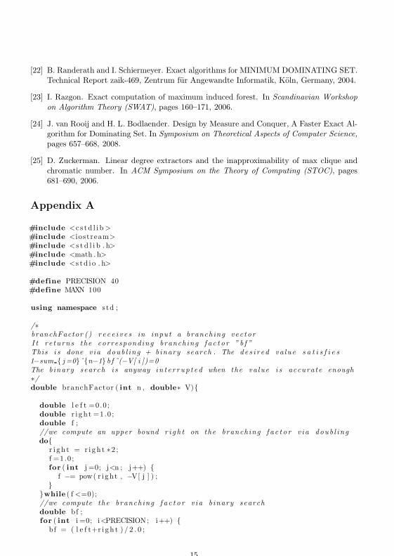
[22] B. Randerath and I. Schiermeyer. Exact algorithms for MINIMUM DOMINATING SET.Technical Report zaik-469, Zentrum fur Angewandte Informatik, Koln, Germany, 2004.

[23] I. Razgon. Exact computation of maximum induced forest. In Scandinavian Workshopon Algorithm Theory (SWAT), pages 160–171, 2006.

[24] J. van Rooij and H. L. Bodlaender. Design by Measure and Conquer, A Faster Exact Al-gorithm for Dominating Set. In Symposium on Theoretical Aspects of Computer Science,pages 657–668, 2008.

[25] D. Zuckerman. Linear degree extractors and the inapproximability of max clique andchromatic number. In ACM Symposium on the Theory of Computing (STOC), pages681–690, 2006.

Appendix A

#include <c s td l i b >#include <iostream>#include <s t d l i b . h>#include <math . h>#include <s td i o . h>

#define PRECISION 40#define MAXN 100

using namespace s td ;

/∗branchFactor ( ) r e c e i v e s in input a branching vec t orI t r e tu rns the corresponding branching f a c t o r ” b f ”This i s done v ia doub l ing + binary search . The de s i r e d va lu e s a t i s f i e s1−sum j =0ˆn−1 b f ˆ(−V[ i ])=0The binary search i s anyway in t e r r u p t e d when the va lu e i s accurate enough∗/double branchFactor ( int n , double∗ V)

double l e f t =0.0 ;double r i g h t =1.0 ;double f ;//we compute an upper bound r i g h t on the branching f a c t o r v ia doub l ingdo

r i g h t = r i g h t ∗2 ;f =1.0 ;for ( int j =0; j<n ; j++)

f −= pow( r i ght , −V[ j ] ) ;

while ( f <=0);//we compute the branching f a c t o r v ia b inary searchdouble bf ;for ( int i =0; i<PRECISION; i++)

bf = ( l e f t+r i g h t ) / 2 . 0 ;

15

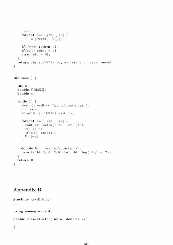
f =1.0 ;for ( int j =0; j<n ; j++)

f −= pow( bf , −V[ j ] ) ;i f ( f==0) return bf ;i f ( f >0) r i g h t = bf ;else l e f t = bf ;

return r i g h t ; // t h i s way we return an upper bound

int main ( )

int n ;double V[MAXN] ;double d ;

while (1 ) cout << endl << ”# o f branchings : ” ;c in >> n ;i f (n<=0 | | n>MAXN) e x i t ( 1 ) ;

for ( int i =0; i<n ; i++) cout << ” de l t a ( ” << i << ” ) : ” ;c in >> d ;i f (d<0) e x i t ( 1 ) ;V[ i ]=d ;

double bf = branchFactor (n , V) ;p r i n t f ( ” bf=%.8 f (%.8 f )\n” , bf , l o g ( bf )/ l og ( 2 ) ) ;

return 0 ;

Appendix B

#include <s t d l i b . h>. . .

using namespace s td ;

double branchFactor ( int n , double∗ V). . .

16

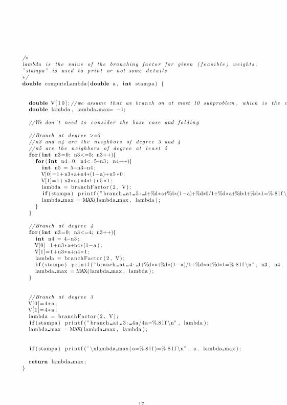
/∗lambda i s the va lu e o f the branching f a c t o r f o r g iven ( f e a s i b l e ) we igh t s .”stampa” i s used to p r in t or not some d e t a i l s∗/double computeLambda(double a , int stampa )

double V[ 1 0 ] ; //we assume t ha t we branch on at most 10 subproblem , which i s the case heredouble lambda , lambda max= −1;

//We don ’ t need to cons ider the base case and f o l d i n g

//Branch at degree >=5//n3 and n4 are the ne ighbor s o f degree 3 and 4//n5 are the ne ighbor s o f degree at l e a s t 5for ( int n3=0; n3<=5; n3++)

for ( int n4=0; n4<=5−n3 ; n4++)int n5 = 5−n3−n4 ;V[0]=1+n3∗a+n4∗(1−a)+n5 ∗0 ;V[1]=1+n3∗a+n4∗1+n5 ∗1 ;lambda = branchFactor (2 , V) ;i f ( stampa ) p r i n t f ( ”branch at 5 : 1+%d∗a+%d∗(1−a)+%d∗0/1+%d∗a+%d∗1+%d∗1=%.8 l f \n” , n3 ,lambda max = MAX( lambda max , lambda ) ;

//Branch at degree 4for ( int n3=0; n3<=4; n3++)

int n4 = 4−n3 ;V[0]=1+n3∗a+n4∗(1−a ) ;V[1]=1+n3∗a+n4 ∗1 ;lambda = branchFactor (2 , V) ;i f ( stampa ) p r i n t f ( ”branch at 4 : 1+%d∗a+%d∗(1−a)/1+%d∗a+%d∗1=%.8 l f \n” , n3 , n4 , n3 , n4 ,lambda max = MAX( lambda max , lambda ) ;

//Branch at degree 3V[0]=4∗a ;V[1 ]=4∗a ;lambda = branchFactor (2 , V) ;i f ( stampa ) p r i n t f ( ”branch at 3 : 4a/4a=%.8 l f \n” , lambda ) ;lambda max = MAX( lambda max , lambda ) ;

i f ( stampa ) p r i n t f ( ”\nlambda max ( a=%.8 l f )=%.8 l f \n” , a , lambda max ) ;

return lambda max ;

17

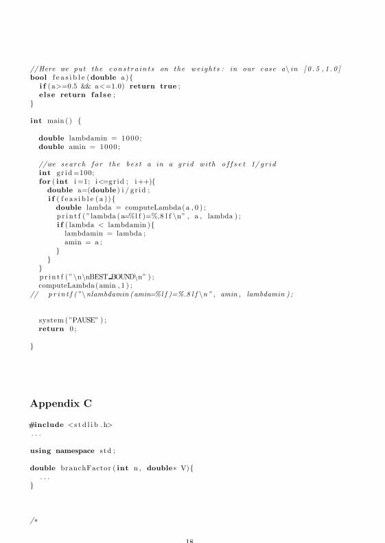
//Here we put the con s t r a in t s on the we igh t s : in our case a\ in [ 0 . 5 , 1 . 0 ]bool f e a s i b l e (double a )

i f ( a>=0.5 && a<=1.0) return true ;else return fa l se ;

int main ( )

double lambdamin = 1000 ;double amin = 1000 ;

//we search f o r the b e s t a in a g r i d wi th o f f s e t 1/ g r i dint g r id =100;for ( int i =1; i<=gr id ; i++)

double a=(double ) i / g r id ;i f ( f e a s i b l e ( a ) )

double lambda = computeLambda(a , 0 ) ;p r i n t f ( ”lambda ( a=%l f )=%.8 l f \n” , a , lambda ) ;i f ( lambda < lambdamin )

lambdamin = lambda ;amin = a ;

p r i n t f ( ”\n\nBEST BOUND\n” ) ;computeLambda(amin , 1 ) ;

// p r i n t f (”\nlambdamin (amin=%l f )=%.8 l f \n” , amin , lambdamin ) ;

system ( ”PAUSE” ) ;return 0 ;

Appendix C

#include <s t d l i b . h>. . .

using namespace s td ;

double branchFactor ( int n , double∗ V). . .

/∗

18

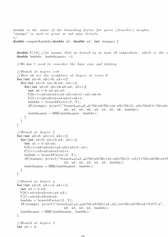
lambda i s the va lu e o f the branching f a c t o r f o r g iven ( f e a s i b l e ) we igh t s .”stampa” i s used to p r in t or not some d e t a i l s∗/double computeLambda(double a3 , double a4 , int stampa )

double V[ 1 0 ] ; //we assume t ha t we branch on at most 10 subproblem , which i s the case heredouble lambda , lambda max= −1;

//We don ’ t need to cons ider the base case and f o l d i n g

//Branch at degree >=6//Here n6 are the ne ighbor s o f degree at l e a s t 6for ( int n3=0; n3<=6; n3++)

for ( int n4=0; n4<=6−n3 ; n4++)for ( int n5=0; n5<=6−n3−n4 ; n5++)

int n6 = 6−n3−n4−n5 ;V[0]=1+n3∗a3+n4∗( a4−a3)+n5∗(1−a4)+n6 ∗0 ;V[1]=1+n3∗a3+n4∗a4+n5∗1+n6 ∗1 ;lambda = branchFactor (2 , V) ;i f ( stampa ) p r i n t f ( ”branch at 6 : 1+%d∗a3+%d∗( a4−a3)+%d∗(1−a4)+%d∗0/1+%d∗a3+%d∗a4+%d

n3 , n4 , n5 , n6 , n3 , n4 , n5 , n6 , lambda ) ;lambda max = MAX( lambda max , lambda ) ;

//Branch at degree 5for ( int n3=0; n3<=5; n3++)

for ( int n4=0; n4<=5−n3 ; n4++)int n5 = 5−n3−n4 ;V[0]=1+n3∗a3+n4 ∗( a4−a3)+n5∗(1−a4 ) ;V[1]=1+n3∗a3+n4∗a4+n5 ∗1 ;lambda = branchFactor (2 , V) ;i f ( stampa ) p r i n t f ( ”branch at 5 : 1+%d∗a3+%d∗( a4−a3)+%d∗(1−a4)/1+%d∗a3+%d∗a4+%d∗1=%.8

n3 , n4 , n5 , n3 , n4 , n5 , lambda ) ;lambda max = MAX( lambda max , lambda ) ;

//Branch at degree 4for ( int n3=0; n3<=4; n3++)

int n4 = 4−n3 ;V[0 ]= a4+n3∗a3+n4∗( a4−a3 ) ;V[1 ]= a4+n3∗a3+n4∗a4 ;lambda = branchFactor (2 , V) ;i f ( stampa ) p r i n t f ( ”branch at 4 : a4+%d∗a3+%d∗( a4−a3 )/ a4+%d∗a3+%d∗a4=%.8 l f \n” ,

n3 , n4 , n3 , n4 , lambda ) ;lambda max = MAX( lambda max , lambda ) ;

//Branch at degree 3int n3 = 3 ;

19

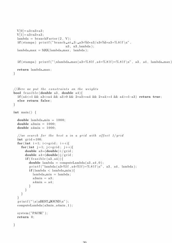
V[0]= a3+n3∗a3 ;V[1 ]= a3+n3∗a3 ;lambda = branchFactor (2 , V) ;i f ( stampa ) p r i n t f ( ”branch at 3 : a3+%d∗a3/a3+%d∗a3=%.8 l f \n” ,

n3 , n3 , lambda ) ;lambda max = MAX( lambda max , lambda ) ;

i f ( stampa ) p r i n t f ( ”\nlambda max ( a3=%.8 l f , a4=%.8 l f )=%.8 l f \n” , a3 , a4 , lambda max ) ;

return lambda max ;

//Here we put the con s t r a in t s on the we igh t sbool f e a s i b l e (double a3 , double a4 )

i f ( a4<=1 && a3<=a4 && a3>0 && 2∗a3>=a4 && 2∗a4>=1 && a4>=1−a3 ) return true ;else return fa l se ;

int main ( )

double lambda min = 1000 ;double a3min = 1000 ;double a4min = 1000 ;

//we search f o r the b e s t a in a g r i d wi th o f f s e t 1/ g r i dint g r id =100;for ( int i =1; i<=gr id ; i++)

for ( int j =1; j<=gr id ; j++)double a3=(double ) i / g r id ;double a4=(double ) j / g r id ;i f ( f e a s i b l e ( a3 , a4 ) )

double lambda = computeLambda( a3 , a4 , 0 ) ;p r i n t f ( ” lambda ( a3=%l f , a4=%l f )=%.8 l f \n” , a3 , a4 , lambda ) ;i f ( lambda < lambda min )

lambda min = lambda ;a3min = a3 ;a4min = a4 ;

p r i n t f ( ”\n\nBEST BOUND\n” ) ;computeLambda( a3min , a4min , 1 ) ;

system ( ”PAUSE” ) ;return 0 ;

20

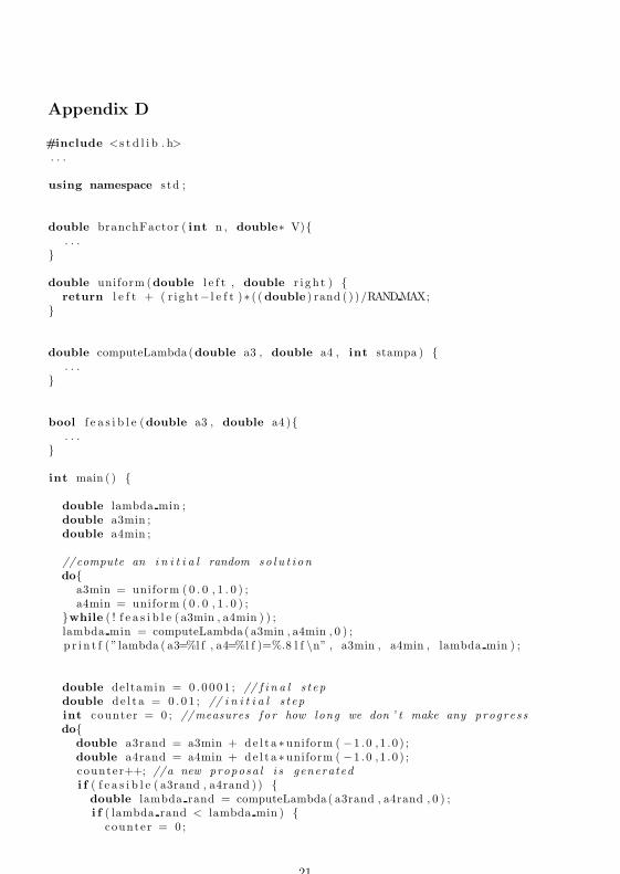
Appendix D

#include <s t d l i b . h>. . .

using namespace s td ;

double branchFactor ( int n , double∗ V). . .

double uniform (double l e f t , double r i g h t ) return l e f t + ( r i ght− l e f t )∗ ( ( double ) rand ( ) ) /RANDMAX;

double computeLambda(double a3 , double a4 , int stampa ) . . .

bool f e a s i b l e (double a3 , double a4 ). . .

int main ( )

double lambda min ;double a3min ;double a4min ;

//compute an i n i t i a l random s o l u t i o ndo

a3min = uniform ( 0 . 0 , 1 . 0 ) ;a4min = uniform ( 0 . 0 , 1 . 0 ) ;

while ( ! f e a s i b l e ( a3min , a4min ) ) ;lambda min = computeLambda ( a3min , a4min , 0 ) ;p r i n t f ( ” lambda ( a3=%l f , a4=%l f )=%.8 l f \n” , a3min , a4min , lambda min ) ;

double deltamin = 0 . 0 0 0 1 ; // f i n a l s t epdouble de l t a = 0 . 0 1 ; // i n i t i a l s t epint counter = 0 ; //measures f o r how long we don ’ t make any progre s sdo

double a3rand = a3min + de l t a ∗uniform ( −1 .0 , 1 . 0 ) ;double a4rand = a4min + de l t a ∗uniform ( −1 .0 , 1 . 0 ) ;counter++; //a new proposa l i s generatedi f ( f e a s i b l e ( a3rand , a4rand ) )

double lambda rand = computeLambda( a3rand , a4rand , 0 ) ;i f ( lambda rand < lambda min )

counter = 0 ;

21

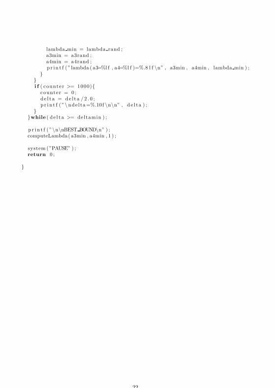
lambda min = lambda rand ;a3min = a3rand ;a4min = a4rand ;p r i n t f ( ” lambda ( a3=%l f , a4=%l f )=%.8 l f \n” , a3min , a4min , lambda min ) ;

i f ( counter >= 1000)

counter = 0 ;d e l t a = de l t a / 2 . 0 ;p r i n t f ( ”\ nde l ta =%.10 f \n\n” , d e l t a ) ;

while ( d e l t a >= deltamin ) ;

p r i n t f ( ”\n\nBEST BOUND\n” ) ;computeLambda( a3min , a4min , 1 ) ;

system ( ”PAUSE” ) ;return 0 ;

22

Thore Husfeldt

A Taxonomic Introductionto Exact Algorithms

A Taxonomic Introduction to Exact Algorithms

Thore Husfeldt

Lecture notes for AGAPE 2009 Spring School on Fixed Parameter andExact Algorithms, May 25-29 2009, Lozari, Corsica (France).1

This document attempts to survey techniques that appear in exact,exponential-time algorithmics using the taxonomy developed by Lev-itin. The purpose is to force the exposition to adopt an alternative per-spective over previous surveys, and to form an opinion of the flexibilityof Levitin’s framework. I have made no attempt to be comprehensive.

1Alpha release from 19 maj 2009. Errors are to be expected, and there are no references. Proceedwith caution.

1

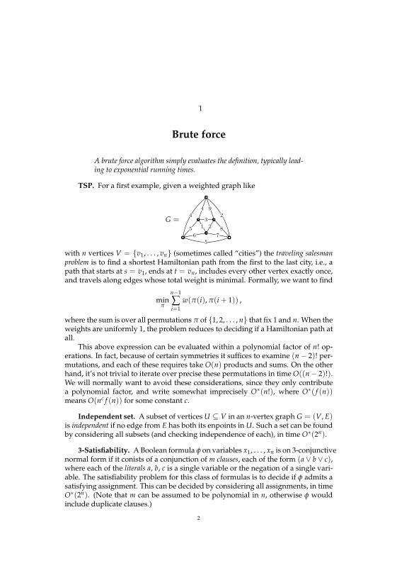
1

Brute force

A brute force algorithm simply evaluates the definition, typically lead-ing to exponential running times.

TSP. For a first example, given a weighted graph like

G =1 2

3

4

5

6 7

8

9

4

5

2

with n vertices V = v1, . . . , vn (sometimes called “cities”) the traveling salesmanproblem is to find a shortest Hamiltonian path from the first to the last city, i.e., apath that starts at s = v1, ends at t = vn, includes every other vertex exactly once,and travels along edges whose total weight is minimal. Formally, we want to find

minπ

n−1

∑i=1

w(π(i), π(i + 1)) ,

where the sum is over all permutations π of 1, 2, . . . , n that fix 1 and n. When theweights are uniformly 1, the problem reduces to deciding if a Hamiltonian path atall.

This above expression can be evaluated within a polynomial factor of n! op-erations. In fact, because of certain symmetries it suffices to examine (n− 2)! per-mutations, and each of these requires take O(n) products and sums. On the otherhand, it’s not trivial to iterate over precise these permutations in time O((n− 2)!).We will normally want to avoid these considerations, since they only contributea polynomial factor, and write somewhat imprecisely O∗(n!), where O∗( f (n))means O(nc f (n)) for some constant c.

Independent set. A subset of vertices U ⊆ V in an n-vertex graph G = (V, E)is independent if no edge from E has both its enpoints in U. Such a set can be foundby considering all subsets (and checking independence of each), in time O∗(2n).

3-Satisfiability. A Boolean formula φ on variables x1, . . . , xn is on 3-conjunctivenormal form if it conists of a conjunction of m clauses, each of the form (a ∨ b ∨ c),where each of the literals a, b, c is a single variable or the negation of a single vari-able. The satisfiability problem for this class of formulas is to decide if φ admits asatisfying assignment. This can be decided by considering all assignments, in timeO∗(2n). (Note that m can be assumed to be polynomial in n, otherwise φ wouldinclude duplicate clauses.)

2

1. BRUTE FORCE 3

FIGURE 1. A bipartite graph and 2 of its 3 perfect matchings.

Perfect matchings. A perfect matching in a graph G = (V, E) is an edge subsetM ⊆ E that includes every vertex as an endpoint exactly once; in other words

|M| = 12 |V|

⋃M = V.

In fact, famously, a matching can be found in polynomial time, so we are inter-ested in the counting version of this problem: how many perfect matchings doesG admit? From the definition, this still takes O∗(2m) time.

We will look at this problem for bipartite graphs as well as for general graphs.

These are all difficult problems, typically hard for NP or # P, so we cannotexpect to devise algorithms that run in polynomial time. Instead, we will improvethe exponential running time. For example, for some problems we will find vertex-exponential time algorithms, i.e., algorithms with running time exp(O(n)) insteadof exp(O(m)) or O∗(n!) O∗(nn). Other algorithms will improve the base of theexponent, for example from O∗(2n) to O(1.732n).

2

Greedy

A greedy algorithm does “the obvious thing” for a given ordering, thehard part is figuring out which ordering. A canonical example isinterval scheduling.

In exponential time, we can consider all orderings. This leads torunning times around n! and is seldom better than brute force, so thisclass of algorithms does not seem to play a role in exponential timealgorithmics. An important exception is given as an exercise.

4

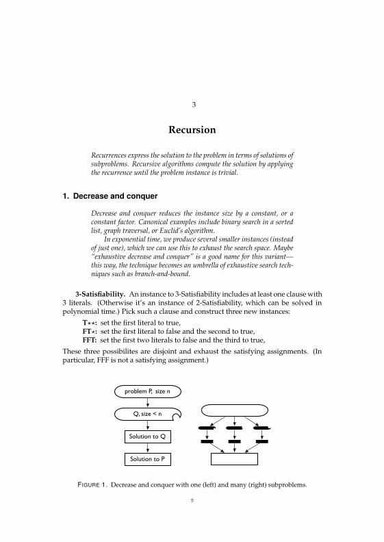
3

Recursion

Recurrences express the solution to the problem in terms of solutions ofsubproblems. Recursive algorithms compute the solution by applyingthe recurrence until the problem instance is trivial.

1. Decrease and conquer

Decrease and conquer reduces the instance size by a constant, or aconstant factor. Canonical examples include binary search in a sortedlist, graph traversal, or Euclid’s algorithm.

In exponential time, we produce several smaller instances (insteadof just one), which we can use this to exhaust the search space. Maybe“exhaustive decrease and conquer” is a good name for this variant—this way, the technique becomes an umbrella of exhaustive search tech-niques such as branch-and-bound.

3-Satisfiability. An instance to 3-Satisfiability includes at least one clause with3 literals. (Otherwise it’s an instance of 2-Satisfiability, which can be solved inpolynomial time.) Pick such a clause and construct three new instances:

T??: set the first literal to true,FT?: set the first literal to false and the second to true,FFT: set the first two literals to false and the third to true,

These three possibilites are disjoint and exhaust the satisfying assignments. (Inparticular, FFF is not a satisfying assignment.)

Q, size < n

problem P, size n

Solution to Q

Solution to P

FIGURE 1. Decrease and conquer with one (left) and many (right) subproblems.

5

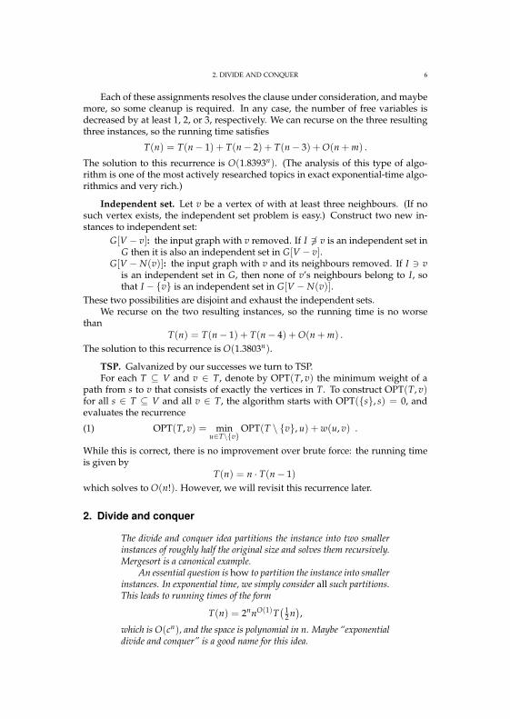
2. DIVIDE AND CONQUER 6

Each of these assignments resolves the clause under consideration, and maybemore, so some cleanup is required. In any case, the number of free variables isdecreased by at least 1, 2, or 3, respectively. We can recurse on the three resultingthree instances, so the running time satisfies

T(n) = T(n− 1) + T(n− 2) + T(n− 3) + O(n + m) .

The solution to this recurrence is O(1.8393n). (The analysis of this type of algo-rithm is one of the most actively researched topics in exact exponential-time algo-rithmics and very rich.)

Independent set. Let v be a vertex of with at least three neighbours. (If nosuch vertex exists, the independent set problem is easy.) Construct two new in-stances to independent set:

G[V − v]: the input graph with v removed. If I 63 v is an independent set inG then it is also an independent set in G[V − v].

G[V − N(v)]: the input graph with v and its neighbours removed. If I 3 vis an independent set in G, then none of v’s neighbours belong to I, sothat I − v is an independent set in G[V − N(v)].

These two possibilities are disjoint and exhaust the independent sets.We recurse on the two resulting instances, so the running time is no worse

thanT(n) = T(n− 1) + T(n− 4) + O(n + m) .

The solution to this recurrence is O(1.3803n).

TSP. Galvanized by our successes we turn to TSP.For each T ⊆ V and v ∈ T, denote by OPT(T, v) the minimum weight of a

path from s to v that consists of exactly the vertices in T. To construct OPT(T, v)for all s ∈ T ⊆ V and all v ∈ T, the algorithm starts with OPT(s, s) = 0, andevaluates the recurrence

(1) OPT(T, v) = minu∈T\v

OPT(T \ v, u) + w(u, v) .

While this is correct, there is no improvement over brute force: the running timeis given by

T(n) = n · T(n− 1)which solves to O(n!). However, we will revisit this recurrence later.

2. Divide and conquer

The divide and conquer idea partitions the instance into two smallerinstances of roughly half the original size and solves them recursively.Mergesort is a canonical example.

An essential question is how to partition the instance into smallerinstances. In exponential time, we simply consider all such partitions.This leads to running times of the form

T(n) = 2nnO(1)T( 1

2 n),

which is O(cn), and the space is polynomial in n. Maybe “exponentialdivide and conquer” is a good name for this idea.

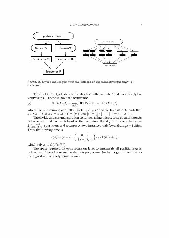
2. DIVIDE AND CONQUER 7

problem P, size n

Q, size n/2 R, size n/2

Solution to Q Solution to R

Solution to P

problem P, size n

Solution to P

...

...

FIGURE 2. Divide and conquer with one (left) and an exponential number (right) ofdivisions.

TSP. Let OPT(U, s, t) denote the shortest path from s to t that uses exactly thevertives in U. Then we have the recurrence

(2) OPT(U, s, t) = minm,S,T

OPT(S, s, m) + OPT(T, m, t) ,

where the minimum is over all subsets S, T ⊆ U and vertices m ∈ U such thats ∈ S, t ∈ T, S ∪ T = U, S ∩ T = m, and |S| = b 1

2 nc+ 1, |T| = n− |S|+ 1.The divide and conquer solution continues using this recurrence until the sets

U become trivial. At each level of the recursion, the algorithm considers (n −2)( n−2d(n−2)/2e) partitions and recurses on two instances with fewer than 1

2 n + 1 cities.Thus, the running time is

T(n) = (n− 2) ·(

n− 2d(n− 2)/2e

)· 2 · T(n/2 + 1) ,

which solves to O(4nnlog n).The space required on each recursion level to enumerate all partitionings is

polynomial. Since the recursion depth is polynomial (in fact, logarithmic) in n, sothe algorithm uses polynomial space.

4

Transformation

Transformations compute a problem by computing a different problemin its stead.

1. Moebius inversion

For a function f on subsets define

g(X) = ∑Y⊆X

f (Y) .

Thenf (X) = ∑

Y⊆X(−1)|X\Y|g(Y) .

This result is called Moebius inversion, or, in a special case, the principle of inclusion–exclusion. For a proof see Dr. Kaski’s presentation.

TSP. We’ll do Hamiltonian path, because the idea stands cleaner.For X ⊆ V with s, t ∈ X, let g(X) denote the number of walks of length n

from s to t using only vertices from X. (A walk can use the same vertex manytimes, or once, or not at all.) Although it is not obvious, g(X) can be computed inpolynomial time for each X ⊆ V; the value is given in row s and column t of An,where A is the adjacency matrix of G[X].

Now, let f (X) denote the number of walks of length n from s to t that useexactly the vertices from X. In particular, f (V) is the number of Hamiltonianpaths from s to t. By Moebius inversion,

f (V) = ∑Y⊆V

(−1)|V\Y|g(Y) .

so the number of Hamiltonian paths can be counted in time O∗(2n) and polyno-mial space.

To make this work for TSP, we need to handle every total distance separately,details omitted.

Perfect matchings. For Y ⊆ V Let f (Y) denote the number of ways of pick-ing 1

2 n edges using exactly the vertices in Y (all of them); the number of perfectmatchings is then given by f (V). For a moment, let g(Y) denote the number ofways of picking 1

2 n edges using only the vertices in Y (but not necessarily all ofthem). Then, by Moebius inversion

f (V) = ∑Y⊆V

(−1)|V\Y|g(Y) .

8

2. FINDING TRIANGLES 9

Since g(Y) is easy to compute for given Y, we can count the number of perfectmatchings in time O∗(2n).

For bipartite graphs, we can do slightly better. So, let V = L ∪ R with |L| =|R| = 1

2 n and assume all edges have an endpoint in L and an enpoint in R. Now,for Y ⊆ R (rather than Y ⊆ V), let g(Y) denote the number of ways of picking12 n edges using all the vertices in L and some of the vertices in Y, and let f (Y)denote the number of ways of picking 1

2 n edges using all the vertices in L and allthe vertices in Y. Then

f (V) = ∑Y⊆R

(−1)|R\Y|g(Y) ,

in particular, the sum has only 2n/2 terms. For each Y ⊆ R, the value g(Y) is easyenough to compute: if vertex vi ∈ L has di neighbours in R then

g(Y) = d1 · · · dn/2 .

Thus, the total running time is O∗(2n/2) = O(1.732n). See fig. 1 for an example.In fact, this is a famous results in combinatorics, the Ryser formula for the per-

manent, often expressed in terms of a 01-matrix A of dimension k× k as

(3) per A = ∑Y⊆1,...,k

(−1)k−|Y| k

∏i=1

∑j∈Y

Aij.

The connection is that A is the upper right quarter of the adjacency matrix of G.

2. Finding triangles

The number of triangles of undirected d-vertex graph T is given by

16 tr A3 ,

where A denotes the adjacency matrix of T and tr, the trace, is the sum of thediagonal entries. To see this, observe that the ith diagonal entry counts the numberof paths of length 3 from the ith vertex to itself, and each triangle contributes six-fold to such entries (once for every corner, and once for every direction).

To compute A3 = A · A · A we need two matrix multiplications, which takestime O(dω), ω < 3 (see Dr. Kaski’s presentation).

Independent set. We want to find an independent set of size k in G = (V, E),and now we assume for simplicity that 3 divides k.

Construct G′ = (V′, E′), where each vertex v ∈ V′ corresponds to an inde-pendent set in G of size 1

3 k. Two vertices are joined by an edge uv ∈ E′ if theircorresponding sets form an independent set of size 2

3 k. The crucial feature is thata triangle in G′ corresponds to an independent set of size k in G. The graph G′ has( n

k/3) ≤ nk/3 vertices, so the whole algorithm takes time O∗(nωk/3), rather than theobvious (n

k).

2. FINDING TRIANGLES 10

sign + − − − +

X = ∅ 1 2 3 1, 3

1

2

3

4

5

6

7

8

9

10

11

12

FIGURE 1. The input graph has threeperfect matchings, in columns 1, 5, and 12.The first row shows all 12 = 3 · 2 · 2 ways tomap the left vertices to the right. Every rowof the table shows the mappings that avoidvarious vertex subsets X, drawn as . Weomit the rows whose contribution is zero,like X = 1, 2, X = 2, 3 andX = 1, 2, 3. Of particular interest iscolumn 8, which is subtracted twice andlater added again. The entire calculation is12− 4− 2− 4 + 1 + 0 + 0− 0, with isindeed 3.

Perfect matchings. The next example is somewhat more intricate, and usesboth transformations from this section.

We return to perfect matchings, but now in regular graphs. Let G[n = r; m =k] denote the number of induced subgraphs of G with r vertices and k edges. Forsuch a graph, the number of ways to pick 1

2 n edges is kn/2, so we can rewrite

f (V) = ∑Y⊆V

(−1)|V\Y|g(Y) =m

∑k=1

n

∑r=2

(−1)rG[n = r; m = k]kn/2 .

Thus, we have reduced the problem to computing G[n = r; m = k] for given r andk, and we’ll now do this faster than in the obvious 2n iterations.

2. FINDING TRIANGLES 11

We are tempted to do the following: Construct a graph T where every vertexcorresponds to a subgraph of G induced by a vertex subset U ⊆ V with 1

3 r verticesand 1

6 k edges. Two vertices in T are joined by an edge if there are 16 k edges between

their corresponding vertex subsets. Then we would like to argue that every trian-gle in T corresponds to an induced subgraph of G with r edges and k edges. This,of course, doesn’t quite work because (1) the three vertex subsets might overlapand (2) the edges do not necessarily partition into such six equal-sized families.Once identified, these problems are easily adressed.

The construction is as follows. Partition the vertices of G into three sets V0, V1,and V2 of equal size, assuming 3 divides n for readability. Our plan is to build alarge tripartite graph T whose vertices correspond to induced subgraphs of G thatare entirely contained in one the Vi.

Some notation: An induced subraph of G has r1 vertices in V1, k1 edges withboth endpoints in V1, and k12 edges between V1 and V2. Define r2, r3, k2 , k3,k23, and k13 similarly. We will solve the problem of computing G[n = r; m =k] separately for each choice of these parameters such that r1 + r2 + r3 = r andk1 + k2 + k3 + k12 + k23 + k13 = k. We can crudely bound the number of such newproblems by n3 + m6, i.e., a polynomial in the input size.

The tripartite graph T is now defined as follows: There is a vertex for everyinduced subgraph G[U], provided that U is entirely contained in one of the Vi, andcontains exactly ri vertices and ki edges. An edge joins the vertices correspondingto Ui ⊆ Vi and Uj ⊆ Vj if i 6= j and there are exactly kij edges between Ui and Uj

in G. The graph T has at most 3 · 2n/3 vertices and 3 · 22n/3 edges. Every trianglein T uniquely corresponds to an induced subgraph G[U1 ∪U2 ∪U3] in G with theparameters described in the previous paragraph.

The total running time is O∗(nωk/3) = (1.732n).

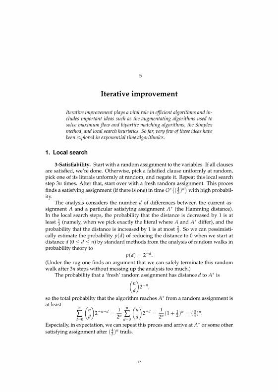
5

Iterative improvement

Iterative improvement plays a vital role in efficient algorithms and in-cludes important ideas such as the augmentating algorithms used tosolve maximum flow and bipartite matching algorithms, the Simplexmethod, and local search heuristics. So far, very few of these ideas havebeen explored in exponential time algorithmics.

1. Local search

3-Satisfiability. Start with a random assignment to the variables. If all clausesare satisfied, we’re done. Otherwise, pick a falsified clause uniformly at random,pick one of its literals unformly at random, and negate it. Repeat this local searchstep 3n times. After that, start over with a fresh random assignment. This procesfinds a satisfying assignment (if there is one) in time O∗

(( 4

3 )n)with high probabil-ity.

The analysis considers the number d of differences between the current as-signment A and a particular satisfying assignment A∗ (the Hamming distance).In the local search steps, the probability that the distance is decreased by 1 is atleast 1

3 (namely, when we pick exactly the literal where A and A∗ differ), and theprobability that the distance is increased by 1 is at most 2

3 . So we can pessimisti-cally estimate the probability p(d) of reducing the distance to 0 when we start atdistance d (0 ≤ d ≤ n) by standard methods from the analysis of random walks inprobability theory to

p(d) = 2−d.(Under the rug one finds an argument that we can safely terminate this randomwalk after 3n steps without messing up the analysis too much.)

The probability that a ‘fresh’ random assignment has distance d to A∗ is(nd

)2−n,

so the total probabilty that the algorithm reaches A∗ from a random assignment isat least

n

∑d=0

(nd

)2−n−d =

12n

n

∑d=0

(nd

)2−d =

12n (1 + 1

2 )n = ( 34 )n.

Especially, in expectation, we can repeat this proces and arrive at A∗ or some othersatisfying assignment after ( 4

3 )n trails.

12

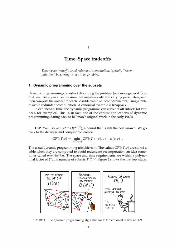
6

Time–Space tradeoffs

Time–space tradeoffs avoid redundant computation, typically “recom-putation,” by storing values in large tables.

1. Dynamic programming over the subsets

Dynamic programming consists of describing the problem (or a more general formof it) recursively in an expression that involves only few varying parameters, andthen compute the answer for each possible value of these parameters, using a tableto avoid redundant computation. A canonical example is Knapsack.

In exponential time, the dynamic programme can consider all subsets (of ver-tices, for example). This is, in fact, one of the earliest applications of dynamicprogramming, dating back to Bellman’s original work in the early 1960s.

TSP. We’ll solve TSP in O(2nn2), a bound that is still the best known. We goback to the decrease and conquer recurrence

OPT(T, v) = minu∈T\v

OPT(T \ v, u) + w(u, v) .

The usual dynamic programming trick kicks in: The values OPT(T, v) are stored atable when they are computed to avoid redundant recomputation, an idea some-times called memoisation. The space and time requirements are within a polyno-mial factor of 2n, the number of subsets T ⊆ V. Figure 2 shows the first few steps.

FIGURE 1. The dynamic programming algorithm for TSP mentioned in xkcd nr. 399.

13

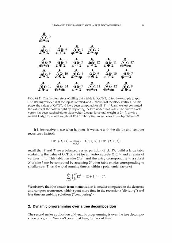
2. DYNAMIC PROGRAMMING OVER A TREE DECOMPOSITION 14

0

4 9 4 2

9 5 7 12 11 17

9 10 9 9 10 7

10 14 7 11 12 9

FIGURE 2. The first few steps of filling out a table for OPT(T, v) for the example graph.The starting vertex s is at the top, v is circled, and T consists of the black vertices. At thisstage, the values of OPT(T, v) have been computed for all |T| ≤ 3, and we just computedthe value 9 at the bottom right by inspecting the two underlined cases. The “new” blackvertex has been reached either via a weight 2 edge, for a total weight of 2 + 7, or via aweight 1 edge for a total weight of 12 + 1. The optimum value for this subproblem is 9.

It is instructive to see what happens if we start with the divide and conquerrecurrence instead:

OPT(U, s, t) = minm,S,T

OPT(S, s, m) + OPT(T, m, t) ;

recall that S and T are a balanced vertex partition of U. We build a large tablecontaining the value of OPT(X, u, v) for all vertex subsets X ⊆ V and all pairs ofvertives u, v. This table has size 2nn2, and the entry corresponding to a subsetX of size k can be computed by accessing 2k other table entries corresponding tosmaller sets. Thus, the total running time is within a polynomial factor of

n

∑k=0

(nk

)2k = (2 + 1)n = 3n.

We observe that the benefit from memoisation is smaller compared to the decreaseand conquer recurrence, which spent more time in the recursion (“dividing”) andless time assembling solutions (“conquering”).

2. Dynamic programming over a tree decomposition

The second major application of dynamic programming is over the tree decompo-sition of a graph. We don’t cover that here, for lack of time.

5. FAST MATRIX MULTIPLICATION 15

3. Meet in the middle

TSP. If the input graph is 4-regular (i.e., every vertex has exactly 4 neigh-bours), it makes sense to enumerate the different Hamiltonian paths by makingone of three choices at every vertex, for a total of at most O∗(3n) paths, instead ofconsidering the O∗(n!) different permutations. Of course, the dynamic program-ming solution is still faster, but we can do even better using a different time–spacetrade-off.

We turn again to the “divide and conquer” recurrence,

OPT(U, s, t) = minm,S,T

OPT(S, s, m) + OPT(T, m, t) .

This time we evaluate it by building a table for all choices of m and T 3 t with|T| = n− b 1

2 nc. No recursion is involved, we brutally check all paths from m tot of length |T|, in time O∗(3n/2). After this table is completed we iterate over allchoices of S 3 s with |S| = b 1

2 nc+ 1 the same way, using 3n/2 iterations. For eachS and m we check our dictionary for the entry corresponding to m and V − T.

It is instructive to compare this idea to the dynamic programming approach.There, we used the recurrence relation at every level. Here, we use it only at thetop. In particular, the meet-in-the-middle idea is qualitatively different from theconcept of using memoisation to save some overlapping recursive invocations.

4. Fast Transforms

→ Dr. Kaski

5. Fast Matrix multiplication

→ Dr. Kaski

7

Exercises

An graph can be k-coloured if each vertex can be coloured with one of k differ-ent colours such that no edge connects vertices of the same colour.

This set of exercises asks you do solve the k-colouring problem in various waysfor a graph with n vertices and m edges

Exercise 1. Using brute force, in time O∗(nk).

Exercise 2. Using a greedy algorithm, in time O∗(n!).

Exercise 3. Using decrease-and-conquer, in time in time O∗(((1 +√

5)/2)n+m).Hint: That’s the solution to the “Finonacci” recurrence T(s) = T(s− 1) + T(s− 2).

Exercise 4. Using divide-and-conquer, in time O∗(9n).

Exercise 5. Using Moebius inversion, in time O∗(3n). Hint: ∑ni=0 (n

i )2i = (2 + 1)n.

Exercise 6. Using dynamic programming over the subsets, in time O∗(3n).

Exercise 7. Using Yates’s algorithm and Moebius inversion, in time O∗(2n).

16

Petteri Kaski

Linear and bilineartransformations for

moderately exponentialalgorithms

LINEAR AND BILINEAR TRANSFORMATIONSFOR MODERATELY EXPONENTIAL ALGORITHMS

(LECTURE NOTES FOR AGAPE 09)

PETTERI KASKI

1. Introduction

Many basic tasks in algebra can be reduced to the problem of evaluating a setof linear or bilinear forms over a ring R (for example, over the integers).

In the linear case, the task is to evaluate

(1) yi =n∑j=1

aijxj for 1 ≤ i ≤ m,

where the aij are coefficients in R, and the xj are elements of R given as input.In the bilinear case, the task is to evaluate

(2) zi =n∑j=1

s∑k=1

bijkxjyk for 1 ≤ i ≤ m,

where the bijk are coefficients in R, and the xj and yk are elements of R given asinput.

Here the coefficients aij and bijk are understood to be static (that is, part ofthe problem definition) and not part of the formal input. Put otherwise, (1) isessentially the task of multiplying a given vector with an implicit m × n matrix,and (2) asks us to evaluate a bilinear product of given two vectors. For example,taking the average 1

n

∑nj=1 xj reduces to (1) with m = 1, and the inner product∑n

j=1 xjyj reduces (2) with m = 1 and n = s.

Exercise 1. Express the task of multiplying two complex numbers, x1 + x2= andy1 + y2=, as the task of evaluating a set of two bilinear forms.

Exercise 2. Express the task of multiplying two polynomials of degrees p and q,respectively, as the task of evaluating a set of p+ q + 1 bilinear forms.

Exercise 3. Express the task of multiplying two matrices of sizes p× q and q × r,respectively, as the task of evaluating a set of p · r bilinear forms.

In this lecture we study algorithms based on “faster-than-obvious” evaluationstrategies for specific linear and bilinear transformations. Our measure of efficiencyin this setting is the number of basic arithmetic operations in the ring R.

Exercise 4. The obvious way to multiply two complex numbers requires four realmultiplications:

(x1 + x2=)(y1 + y2=) = x1y1 − x2y2 + (x1y2 + y1x2)=.Show that three real multiplications suffice.

1

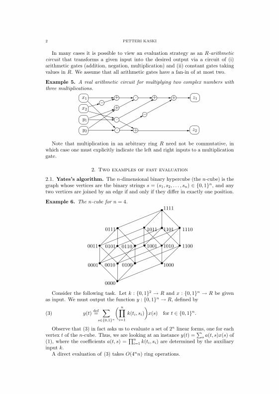
2 PETTERI KASKI

In many cases it is possible to view an evaluation strategy as an R-arithmeticcircuit that transforms a given input into the desired output via a circuit of (i)arithmetic gates (addition, negation, multiplication) and (ii) constant gates takingvalues in R. We assume that all arithmetic gates have a fan-in of at most two.

Example 5. A real arithmetic circuit for multiplying two complex numbers withthree multiplications.

+

+

··

· +

+

x1

x2

y1

y2

+ z1

z2

−

−

Note that multiplication in an arbitrary ring R need not be commutative, inwhich case one must explicitly indicate the left and right inputs to a multiplicationgate.

2. Two examples of fast evaluation

2.1. Yates’s algorithm. The n-dimensional binary hypercube (the n-cube) is thegraph whose vertices are the binary strings s = (s1, s2, . . . , sn) ∈ 0, 1n, and anytwo vertices are joined by an edge if and only if they differ in exactly one position.

Example 6. The n-cube for n = 4.

0001

1001

1000

1111

1010 1100

11101011 1101

0110

01000010

0000

0101

0111

0011

Consider the following task. Let k : 0, 12 → R and x : 0, 1n → R be givenas input. We must output the function y : 0, 1n → R, defined by

(3) y(t) def=∑

s∈0,1n

( n∏i=1

k(ti, si))x(s) for t ∈ 0, 1n.

Observe that (3) in fact asks us to evaluate a set of 2n linear forms, one for eachvertex t of the n-cube. Thus, we are looking at an instance y(t) =

∑s a(t, s)x(s) of

(1), where the coefficients a(t, s) =∏ni=1 k(ti, si) are determined by the auxiliary

input k.A direct evaluation of (3) takes O(4nn) ring operations.

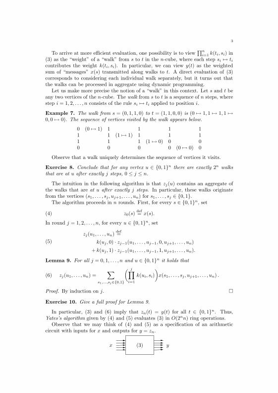
3

To arrive at more efficient evaluation, one possibility is to view∏ni=1 k(ti, si) in

(3) as the “weight” of a “walk” from s to t in the n-cube, where each step si 7→ ticontributes the weight k(ti, si). In particular, we can view y(t) as the weightedsum of “messages” x(s) transmitted along walks to t. A direct evaluation of (3)corresponds to considering each individual walk separately, but it turns out thatthe walks can be processed in aggregate using dynamic programming.

Let us make more precise the notion of a “walk” in this context. Let s and t beany two vertices of the n-cube. The walk from s to t is a sequence of n steps, wherestep i = 1, 2, . . . , n consists of the rule si 7→ ti applied to position i.

Example 7. The walk from s = (0, 1, 1, 0) to t = (1, 1, 0, 0) is (0 7→ 1, 1 7→ 1, 1 7→0, 0 7→ 0). The sequence of vertices visited by the walk appears below.

0 (0 7→ 1) 1 1 1 11 1 (1 7→ 1) 1 1 11 1 1 (1 7→ 0) 0 00 0 0 0 (0 7→ 0) 0

Observe that a walk uniquely determines the sequence of vertices it visits.

Exercise 8. Conclude that for any vertex u ∈ 0, 1n there are exactly 2n walksthat are at u after exactly j steps, 0 ≤ j ≤ n.

The intuition in the following algorithm is that zj(u) contains an aggregate ofthe walks that are at u after exactly j steps. In particular, these walks originatefrom the vertices (s1, . . . , sj , uj+1, . . . , un) for s1, . . . , sj ∈ 0, 1.

The algorithm proceeds in n rounds. First, for every s ∈ 0, 1n, set

(4) z0(s) def= x(s).

In round j = 1, 2, . . . , n, for every u ∈ 0, 1n, set

zj(u1, . . . , un) def=

k(uj , 0) · zj−1(u1, . . . , uj−1, 0, uj+1, . . . , un)

+ k(uj , 1) · zj−1(u1, . . . , uj−1, 1, uj+1, . . . , un).

(5)

Lemma 9. For all j = 0, 1, . . . , n and u ∈ 0, 1n it holds that

(6) zj(u1, . . . , un) =∑

s1,...,sj∈0,1

( j∏i=1

k(ui, si))x(s1, . . . , sj , uj+1, . . . , un) .

Proof. By induction on j.

Exercise 10. Give a full proof for Lemma 9.

In particular, (3) and (6) imply that zn(t) = y(t) for all t ∈ 0, 1n. Thus,Yates’s algorithm given by (4) and (5) evaluates (3) in O(2nn) ring operations.

Observe that we may think of (4) and (5) as a specification of an arithmeticcircuit with inputs for x and outputs for y = zn.

(3)x y

4 PETTERI KASKI

Exercise 11. Draw Yates’s algorithm as an arithmetic circuit when n = 3 andk(0, 0) = 1, k(1, 0) = 1, k(0, 1) = 0, k(1, 1) = 1.

Exercise 12. Let A and B be m×n and p×q matrices, respectively. The Kroneckerproduct A⊗B is the mp× nq matrix defined by

A⊗B def=

a11B a12B · · · a1nBa21B a22B · · · a2nB

......

. . ....

am1B am2B · · · amnB

.Express (3) as a matrix–vector product, where the matrix is obtained via Kroneckerproducts. Using this representation, design a recursive version of Yates’s algorithm.

Exercise 13. Extend Yates’s algorithm to evaluate sums of the formy(t1, . . . , tn) =m1−1∑s1=0

m2−1∑s2=0

· · ·mn−1∑sn=0

k1(t1, . . . , tn, s1)k2(t2, . . . , tn, s2) · · · kn(tn, sn)x(s1, . . . , sn)

where ti = 0, 1, . . . ,mi − 1 for i = 1, 2, . . . n.

Exercise 14. Consider the one-dimensional discrete Fourier transform for a se-quence x(0), x(1), . . . , x(2n − 1) of length 2n:

y(t) =2n−1∑s=0

exp(

2π=st2n

)x(s) for t = 0, 1, . . . , 2n − 1.

Reduce to the form in the previous exercise.

2.2. Strassen’s algorithm. How many multiplications does it take to multiplytwo 2× 2 matrices? A direct evaluation takes 8 multiplications:

X =[a bc d

], Y =

[e fg h

], XY =

[ae+ bg af + bhce+ dg cf + dh

].

However, as was discovered by Strassen in 1968, 7 multiplications suffice:

XY =[q5 + q4 − q2 + q6 q1 + q2

q3 + q4 q1 + q5 − q3 − q7],

where

q1 = a(f − h) , q5 = (a+ d)(e+ h) ,

q2 = (a+ b)h , q6 = (b− d)(g + h) ,

q3 = (c+ d)e , q7 = (a− c)(e+ f) ,

q4 = d(g − e) .Exercise 15. Express Strassen’s formula as an arithmetic circuit with three levelsof gates (addition, multiplication, addition).

Now, suppose we want to multiply two n × n matrices, X and Y . Assuming nis even (if not, insert a row and column of 0s to both matrices), we can partitionX and Y each into four dn/2e × dn/2e submatrices

X =[A BC D

], Y =

[E FG H

]

5

whereby the product XY can be expressed in similarly partitioned form as

XY =[AE +BG AF +BHCE +DG CF +DH

].

Deja vu? Indeed, Strassen’s discovery tells us how to compute the matrix productXY using only 7 multiplications of dn/2e×dn/2e matrices! By recursion, we obtainthat two n× n matrices can be multiplied in

(7) T (n) = 7T (dn/2e) +O(n2)

arithmetic operations, that is, T (n) = O(nlog2 7) = O(n2.81). Computing directlyfrom the definition takes Θ(n3) operations.

Can one do better than O(n2.81)? Put otherwise, for which exponents α dothere exist algorithms such that one can multiply n × n matrices in time O(nα)?Obviously α ≥ 2. Let ω be the greatest lower bound for such exponents α. We saythat ω is the exponent of matrix multiplication. Currently the best upper bound isω ≤ 2.376 (see §5.3), but many conjecture that ω = 2.

3. Transformations on the subset lattice

Let U = 1, 2, . . . , n and denote by 2U the set of all subsets of U . The basic setoperations (A∪B, A∩B, A\B, . . .) on 2U induce natural bilinear transformationson functions f : 2U → R. We study two such transformations, the union productand the disjoint union product.

3.1. The union product. Let f : 2U → R and g : 2U → R. Define the unionproduct f ∪ g : 2U → R by

(8) (f ∪ g)(S) def=∑

A∪B=S

f(A)g(B) for S ⊆ U,

where the sum is understood to range over all pairs A,B ⊆ U such that A∪B = S.Observe that (8) is an instance of (2).

Exercise 16. (f ∪ g) ∪ h = f ∪ (g ∪ h).

Exercise 17. (f1 ∪ f2 ∪ · · · ∪ fk)(S) =∑A1∪A2∪···∪Ak=S f1(A1)f2(A2) · · · fk(Ak).

Exercise 18. For a given S ⊆ U , how many pairs (A,B) are there such thatA ∪B = S? Given f and g as input, how many arithmetic operations does it taketo compute f ∪ g directly from the definition?

3.2. Moebius inversion. The principle of Moebius inversion states that any finitepartially ordered set (X,≤) has a pair of mutually inverse linear transformations,the zeta transform and the Moebius transform, for manipulating functions f : X →R. In particular, this applies to (2U ,⊆), and will reduce f ∪ g into a pointwiseproduct amenable for fast evaluation.

Lemma 19. A finite nonempty set has equally many subsets of even and odd size.

Proof. Let x ∈ U . Partition the subsets of U into pairs by associating S ⊆ U \ xwith S ∪ x. Exactly one set in each pair has even (odd) size.

Exercise 20. Give an algebraic proof for Lemma 19. Hint: the Binomial Theorem(x+ y)n =

∑ni=0

(ni

)xiyn−i.

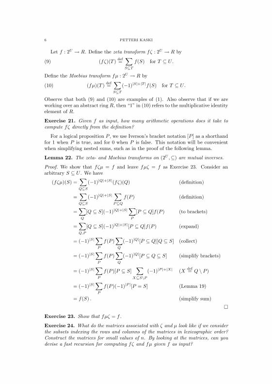
6 PETTERI KASKI

Let f : 2U → R. Define the zeta transform fζ : 2U → R by

(9) (fζ)(T ) def=∑S⊆T

f(S) for T ⊆ U.

Define the Moebius transform fµ : 2U → R by

(10) (fµ)(T ) def=∑S⊆T

(−1)|S|+|T |f(S) for T ⊆ U.

Observe that both (9) and (10) are examples of (1). Also observe that if we areworking over an abstract ring R, then “1” in (10) refers to the multiplicative identityelement of R.

Exercise 21. Given f as input, how many arithmetic operations does it take tocompute fζ directly from the definition?

For a logical proposition P , we use Iverson’s bracket notation [P ] as a shorthandfor 1 when P is true, and for 0 when P is false. This notation will be convenientwhen simplifying nested sums, such as in the proof of the following lemma.

Lemma 22. The zeta- and Moebius transforms on (2U ,⊆) are mutual inverses.

Proof. We show that fζµ = f and leave fµζ = f as Exercise 23. Consider anarbitrary S ⊆ U . We have

(fζµ)(S) =∑Q⊆S

(−1)|Q|+|S|(fζ)(Q) (definition)

=∑Q⊆S

(−1)|Q|+|S|∑P⊆Q

f(P ) (definition)

=∑Q

[Q ⊆ S](−1)|Q|+|S|∑P

[P ⊆ Q]f(P ) (to brackets)

=∑Q,P

[Q ⊆ S](−1)|Q|+|S|[P ⊆ Q]f(P ) (expand)

= (−1)|S|∑P

f(P )∑Q

(−1)|Q|[P ⊆ Q][Q ⊆ S] (collect)

= (−1)|S|∑P

f(P )∑Q

(−1)|Q|[P ⊆ Q ⊆ S] (simplify brackets)

= (−1)|S|∑P

f(P )[P ⊆ S]∑

X⊆S\P(−1)|P |+|X| (X def= Q \ P )

= (−1)|S|∑P

f(P )(−1)|P |[P = S] (Lemma 19)

= f(S) . (simplify sum)

Exercise 23. Show that fµζ = f .

Exercise 24. What do the matrices associated with ζ and µ look like if we considerthe subsets indexing the rows and columns of the matrices in lexicographic order?Construct the matrices for small values of n. By looking at the matrices, can youdevise a fast recursion for computing fζ and fµ given f as input?

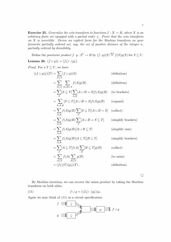
7

Exercise 25. Generalize the zeta transform to functions f : X → R, where X is anarbitrary finite set equipped with a partial order ≤. Prove that the zeta transformon X is invertible. Derive an explicit form for the Moebius transform on yourfavourite partially ordered set, say, the set of positive divisors of the integer n,partially ordered by divisibility.

Define the pointwise product f · g : 2U → R by (f · g)(S) def= f(S)g(S) for S ⊆ U .

Lemma 26. (f ∪ g)ζ = (fζ) · (gζ).

Proof. For a T ⊆ U , we have

((f ∪ g)ζ)(T ) =∑S⊆T

(f ∪ g)(S) (definition)

=∑S⊆T

∑A∪B=S

f(A)g(B) (definition)

=∑S

[S ⊆ T ]∑A,B

[A ∪B = S]f(A)g(B) (to brackets)

=∑S,A,B

[S ⊆ T ][A ∪B = S]f(A)g(B) (expand)

=∑A,B

f(A)g(B)∑S

[S ⊆ T ][A ∪B = S] (collect)

=∑A,B

f(A)g(B)∑S

[A ∪B = S ⊆ T ] (simplify brackets)

=∑A,B

f(A)g(B)[A ∪B ⊆ T ] (simplify sum)

=∑A,B

f(A)g(B)[A ⊆ T ][B ⊆ T ] (simplify brackets)

=∑A

[A ⊆ T ]f(A)∑B

[B ⊆ T ]g(B) (collect)

=∑A⊆T

f(A)∑B⊆T

g(B) (to sums)

= (fζ)(T )(gζ)(T ) . (definition)

By Moebius inversion, we can recover the union product by taking the Moebiustransform on both sides:

(11) f ∪ g = ((fζ) · (gζ))µ .

Again we may think of (11) as a circuit specification:

f ∪ gµ

f ζ

g ζ

·

8 PETTERI KASKI

Exercise 27. (f1 ∪ f2 ∪ · · · ∪ fk)ζ = (f1ζ) · (f2ζ) · . . . · (fkζ).

Exercise 28. How many operations does it take to directly evaluate the right-handside of f ∪ f ∪ · · · ∪ f︸ ︷︷ ︸

k terms

= (fζ)·kµ ? What if we only want (f ∪ f ∪ · · · ∪ f)(U)?

3.3. Disjoint union product (subset convolution). Let us consider a variantof the union product where we require the unions A ∪ B = S to be disjoint, thatis, that A ∩B = ∅ must also hold.

For brevity, let us write A·∪ B = S as a shorthand for A∪B = S and A∩B = ∅.

More generally, let us write A1

·∪ A2

·∪ · · · ·∪ Ak = S for A1 ∪ A2 ∪ · · · ∪ Ak = Sand Ai ∩Aj = ∅ for all 1 ≤ i < j ≤ k.

Define the disjoint union product f·∪ g : 2U → R by

(12) (f·∪ g)(S) def=

∑A·∪B=S

f(A)g(B) for S ⊆ U.

The union product is also called the subset convolution because of the “convolution-like” equivalent form

(f·∪ g)(S) =

∑T⊆S

f(T )g(S \ T ) .

Again observe that (12) is an instance of (2).

Exercise 29. (f·∪ g)

·∪ h = f·∪ (g

·∪ h).

Exercise 30. (f1·∪ f2

·∪ · · · ·∪ fk)(S) =∑A1·∪A2

·∪··· ·∪Ak=Sf1(A1)f2(A2) · · · fk(Ak).

Exercise 31. Given f and g as input, how many arithmetic operations does it taketo compute f

·∪ g directly using the convolution form?

Let us now reduce f·∪ g via “polynomial extension” to the union product. The

following fact will provide the crux of the argument.

Lemma 32. For A,B, S ⊆ U we have A ∪ B = S and A ∩ B = ∅ if and only ifA ∪B = S and |A|+ |B| = |S|.

Let w be a polynomial indeterminate, and denote by R〈w〉 the associated univari-ate polynomial ring with coefficients in R. For a polynomial p =

∑i aiw

i ∈ R〈w〉,denote by wjp the coefficient of the monomial wj in p, that is, wjp = aj .

Exercise 33. Can we use an R-arithmetic circuit to simulate an R〈w〉-arithmeticcircuit? What if we introduce an R〈w〉-arithmetic gate wj that takes as inputa polynomial and outputs (as a polynomial of degree zero) the coefficient of themonomial wj for a constant j?

Exercise 34. Can we replace computations with explicit polynomials by compu-tations with evaluations of such polynomials in sufficiently many distinct pointsw = w0, w1, . . . , wd to enable recovery of the polynomial coefficients (as necessary)via interpolation? Can we interpolate in an arbitrary ring?

Let us now proceed with the reduction. Suppose we are given f : 2U → Rand g : 2U → R as input. Define f 〈w〉 : 2U → R〈w〉 and g〈w〉 : 2U → R〈w〉 byf 〈w〉(S) = f(S)w|S| and g〈w〉(S) = g(S)w|S| for S ⊆ U .

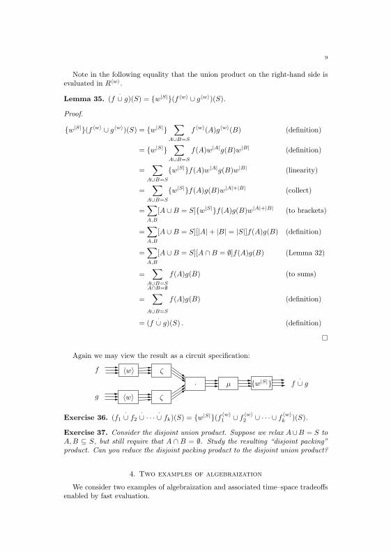
9

Note in the following equality that the union product on the right-hand side isevaluated in R〈w〉.

Lemma 35. (f·∪ g)(S) = w|S|(f 〈w〉 ∪ g〈w〉)(S).

Proof.

w|S|(f 〈w〉 ∪ g〈w〉)(S) = w|S|∑

A∪B=S

f 〈w〉(A)g〈w〉(B) (definition)

= w|S|∑

A∪B=S

f(A)w|A|g(B)w|B| (definition)

=∑

A∪B=S

w|S|f(A)w|A|g(B)w|B| (linearity)

=∑

A∪B=S

w|S|f(A)g(B)w|A|+|B| (collect)

=∑A,B

[A ∪B = S]w|S|f(A)g(B)w|A|+|B| (to brackets)

=∑A,B

[A ∪B = S][|A|+ |B| = |S|]f(A)g(B) (definition)

=∑A,B

[A ∪B = S][A ∩B = ∅]f(A)g(B) (Lemma 32)

=∑

A∪B=SA∩B=∅

f(A)g(B) (to sums)

=∑

A·∪B=S

f(A)g(B) (definition)

= (f·∪ g)(S) . (definition)

Again we may view the result as a circuit specification:

w|S|ζ

ζ

〈w〉

〈w〉g

f

µ· f·∪ g

Exercise 36. (f1·∪ f2

·∪ · · · ·∪ fk)(S) = w|S|(f 〈w〉1 ∪ f 〈w〉2 ∪ · · · ∪ f 〈w〉k )(S).

Exercise 37. Consider the disjoint union product. Suppose we relax A∪B = S toA,B ⊆ S, but still require that A ∩ B = ∅. Study the resulting “disjoint packing”product. Can you reduce the disjoint packing product to the disjoint union product?

4. Two examples of algebraization

We consider two examples of algebraization and associated time–space tradeoffsenabled by fast evaluation.

10 PETTERI KASKI

4.1. Graph coloring. Let G be an undirected loopless graph with vertex set V .A set I ⊆ V is independent in G if no two vertices in I are joined by an edge ofG. We say that G is k-colorable if there exist independent sets I1, I2, . . . , Ik suchthat I1

·∪ I2·∪ · · · ·∪ Ik = V . Such an ordered tuple (I1, I2, . . . , Ik) is a (proper)

k-coloring of G. Indeed, the intuition is that the vertices in Ii have “color” i; acoloring is proper if and only if the ends of every edge have distinct colors.

The k-coloring problem asks, given a graph G and a positive integer k as input,whether G has a proper k-coloring.

4.2. Algebraizing graph coloring. Denote by Z the ring of integers. Let f :2V → Z be the indicator function for independent sets in G, that is, f(I) =[I is independent in G] for I ⊆ V . Note that f is implicitly defined by the inputG.

The number of distinct proper k-colorings of G is, by an iterated application ofthe disjoint union product,

(13)∑

I1·∪I2·∪··· ·∪Ik=V

f(I1)f(I2) · · · f(Ik) = w|V |((f 〈w〉ζ)·kµ)(V ) .

Assuming that |V | = n and k = O(n), a direct evaluation of the right-hand sideof (13) requires O∗(3n) time and O∗(1) space, where O∗(·) hides a multiplicativefactor polynomial in n.

4.3. A time-space tradeoff via fast Moebius inversion. The evaluation ofproduct forms such as (13) can be expedited if sufficient space is available.

Lemma 38. The zeta transform on the subset lattice can be computed in O(2nn)ring operations given space for O(2n) ring elements.

Proof. Recall that we assume U = 1, 2, . . . , n. Identify S ⊆ U with the binarystring s = (s1, s2, . . . , sn) ∈ 0, 1n by i ∈ S if and only if si = 1 for 1 ≤ i ≤ n.In particular, we have [S ⊆ T ] =

∏ni=1[si ≤ ti]. Thus, Yates’s algorithm with

x(s) ← f(S) and k(b, a) ← [a ≤ b] in (3) uses O(2nn) ring operations to compute(fζ)(T ) = y(t) for all T ⊆ U . Storage for O(2n) ring elements suffices because zjdepends only on zj−1 in (5).

Exercise 39. Show that the Moebius transform admits a similar tradeoff.

Theorem 40. The union product can be computed in O(2nn) ring operations givenspace for O(2n) ring elements.

Proof. We take advantage of (11) and Lemma 38. Given f and g as input, computefζ and gζ, take the pointwise product (fζ) · (gζ), and finally compute the Moebiustransform ((fζ) · (gζ))µ to obtain f ∪ g. Each of the three steps takes O(2nn)operations.

Exercise 41. Show that the disjoint union product can be computed in O(2nn2)ring operations given space for O(2n) ring elements.

Thus, given O∗(2n) space, we can solve graph coloring in O∗(2n) time by evalu-ating the right-hand side of (13).

Exercise 42. Can you give other examples of natural “partitioning problems” thatcan be solved using product forms such as (13)?

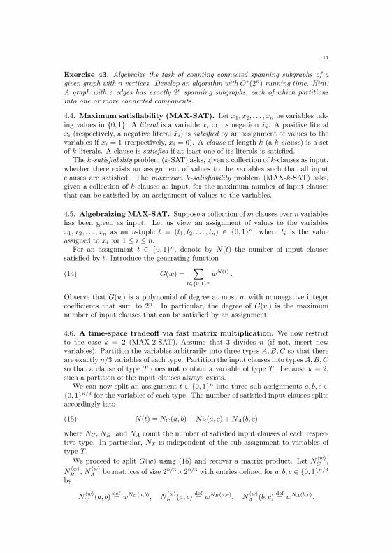
11

Exercise 43. Algebraize the task of counting connected spanning subgraphs of agiven graph with n vertices. Develop an algorithm with O∗(2n) running time. Hint:A graph with e edges has exactly 2e spanning subgraphs, each of which partitionsinto one or more connected components.

4.4. Maximum satisfiability (MAX-SAT). Let x1, x2, . . . , xn be variables tak-ing values in 0, 1. A literal is a variable xi or its negation xi. A positive literalxi (respectively, a negative literal xi) is satisfied by an assignment of values to thevariables if xi = 1 (respectively, xi = 0). A clause of length k (a k-clause) is a setof k literals. A clause is satisfied if at least one of its literals is satisfied.

The k-satisfiability problem (k-SAT) asks, given a collection of k-clauses as input,whether there exists an assignment of values to the variables such that all inputclauses are satisfied. The maximum k-satisfiability problem (MAX-k-SAT) asks,given a collection of k-clauses as input, for the maximum number of input clausesthat can be satisfied by an assignment of values to the variables.

4.5. Algebraizing MAX-SAT. Suppose a collection of m clauses over n variableshas been given as input. Let us view an assignment of values to the variablesx1, x2, . . . , xn as an n-tuple t = (t1, t2, . . . , tn) ∈ 0, 1n, where ti is the valueassigned to xi for 1 ≤ i ≤ n.

For an assignment t ∈ 0, 1n, denote by N(t) the number of input clausessatisfied by t. Introduce the generating function

(14) G(w) =∑

t∈0,1n

wN(t) .

Observe that G(w) is a polynomial of degree at most m with nonnegative integercoefficients that sum to 2n. In particular, the degree of G(w) is the maximumnumber of input clauses that can be satisfied by an assignment.

4.6. A time-space tradeoff via fast matrix multiplication. We now restrictto the case k = 2 (MAX-2-SAT). Assume that 3 divides n (if not, insert newvariables). Partition the variables arbitrarily into three types A,B,C so that thereare exactly n/3 variables of each type. Partition the input clauses into types A,B,Cso that a clause of type T does not contain a variable of type T . Because k = 2,such a partition of the input clauses always exists.

We can now split an assignment t ∈ 0, 1n into three sub-assignments a, b, c ∈0, 1n/3 for the variables of each type. The number of satisfied input clauses splitsaccordingly into

(15) N(t) = NC(a, b) +NB(a, c) +NA(b, c)

where NC , NB , and NA count the number of satisfied input clauses of each respec-tive type. In particular, NT is independent of the sub-assignment to variables oftype T .

We proceed to split G(w) using (15) and recover a matrix product. Let N 〈w〉C ,N〈w〉B , N 〈w〉A be matrices of size 2n/3×2n/3 with entries defined for a, b, c ∈ 0, 1n/3

by

N〈w〉C (a, b) def= wNC(a,b), N

〈w〉B (a, c) def= wNB(a,c), N

〈w〉A (b, c) def= wNA(b,c).

12 PETTERI KASKI

We now have

G(w) =∑a,b,c

wNC(a,b)+NB(a,c)+NA(b,c) (split to types)

=∑a,b,c

wNC(a,b)wNB(a,c)wNA(b,c) (expand)

=∑a,c

wNB(a,c)∑b

wNC(a,b)wNA(b,c) (collect)(16)

=∑a,c

N〈w〉B (a, c)

∑b

N〈w〉C (a, b)N 〈w〉A (b, c) (in matrix form)

=∑a,c

N〈w〉B (a, c)

(N〈w〉C N

〈w〉A

)(a, c). (to matrix product)

A trivial algorithm for MAX-2-SAT runs in O∗(2n) time and O∗(1) space. Using(16), we can now trade space for time by first constructing the matrices N 〈w〉C , N 〈w〉B ,N〈w〉A and then using fast matrix multiplication to determine the product N 〈w〉C N

〈w〉A

in O((2n/3)ω+ε) ring operations for any fixed ε > 0, which leads to O∗(2(ω+ε)n/3)time and O∗(22n/3) space for MAX-2-SAT.

Exercise 44. Observe that one can carry out the computations in (16) with evalu-ations of the generating function G(w) at m+1 distinct points w = w0, w1, . . . , wm,and then recover G(w) via interpolation.

5. Further exercises and remarks

5.1. Transforms on the subset lattice. The following exercises develop andrelate to each other some further transformations on the subset lattice.

Define the up-zeta transform fζ ′ : 2U → R by

fζ ′(T ) def=∑T⊆S

f(S) for T ⊆ U .

Define the up-Moebius transform fµ′ : 2U → R by

fµ′(T ) def=∑T⊆S

(−1)|S|+|T |f(S) for T ⊆ U .

Exercise 45. Observe that in matrix form we obtain ζ ′ from ζ by taking the trans-pose. Similarly for µ′ and µ.

Define the complement transform fκ : 2U → R by

(fκ)(S) def= f(U \ S) for S ⊆ U.Define the odd-negation transform fσ : 2U → R by

(fσ)(S) def= (−1)|S|f(S) for S ⊆ U.Exercise 46. ζ ′ = κζκ, µ′ = κµκ, µ = σζσ, ζ = σµσ.

Exercise 47. ζ ′µ = ζκσ, ζµ′ = ζ ′σκ, µ′ζ = µσκ, µζ ′ = µ′κσ.

Exercise 48. Present a natural definition for δ def= ζκ. Show that δ = ζ ′σζ.

13

Exercise 49. Define the intersection product f ∩ g : 2U → R by (f ∩ g)(S) def=∑A∩B=S f(A)g(B) for S ⊆ U . Show that (f ∩ g)κ = (fκ)∪ (fκ). Take the up-zeta

transform of f ∩ g and simplify to a pointwise product. Establish (f ∩ g) ∩ h =f ∩ (g ∩ h).

Exercise 50. Define the difference product f \ g : 2U → R by (f \ g)(S) def=∑A\B=S f(A)g(B) for S ⊆ U . Show that f \ g = f ∩ (gκ).

Exercise 51. Define the Walsh–Hadamard transform (the Fourier transform onthe n-cube) fφ : 2U → R by (fφ)(S) def=

∑T (−1)|S∩T |f(T ) for S ⊆ U . Show that

fφ2 = 2nf . Is φ invertible if R is an arbitrary ring?

Exercise 52. For A,B ⊆ U , define the symmetric difference A⊕ B def= (A \ B) ∪(B \A). Define the symmetric difference product f ⊕ g : 2U → R by (f ⊕ g)(S) def=∑A⊕B=S f(A)g(B) for S ⊆ U . Show that (f ⊕ g)φ = (fφ) · (gφ). Establish

(f ⊕ g)⊕ h = f ⊕ (g ⊕ h).

Exercise 53. Reduce the disjoint union product to the symmetric difference prod-uct.

Exercise 54. Let f : 2U → R and k : 2U → R. Define the k-intersection transformfτ∩k : 2U → R by (fτ∩k )(S) =

∑T k(S ∩ T )f(T ) for S ⊆ U . Show that fτ∩k =

((kµ) · (fζ ′))ζ.

Exercise 55. Observe that φ reduces to τ∩k for a specific k. Simplify the pointwiseproduct form of the k-intersection product when k is 1 on sets of size j, and 0elsewhere.

Exercise 56. Define similar k-union, k-difference, and k-symmetric differencetransforms. Reduce each to a pointwise product form.

Exercise 57. Are all the transforms in this section computable in O∗(2n) ringoperations given space for O∗(2n) ring elements?

5.2. Trimming. This section investigates “trimming” of transforms on 2U whenthe input and output are restricted to subsets of 2U .

Our first objective is a “closure trimming lemma” for fast Moebius inversion.Let F ⊆ 2U . Denote by ↑F the up-closure of F, that is, the set consisting of

the sets in F and all their supersets in 2U . Denote by ↓F the down-closure of F,that is, the set consisting of the sets in F and all their subsets in 2U . Define theelementwise complement of F by U\F def= U\S : S ∈ F.Exercise 58. U\↑F = ↓U\F, U\↓F = ↑U\F.

Lemma 59. There exist algorithms that, given E ⊆ 2U and F ⊆ 2U as input,construct an R-arithmetic circuit with input gates for f : F → R and output gatesthat evaluate to any of fζ : E → R, fζ ′ : E → R, fµ : E → R, or fµ′ : E → R,with construction time any of O∗(|↑E|+ |↑F|), O∗(|↑E|+ |↓F|), O∗(|↓E|+ |↑F|), orO∗(|↓E|+ |↓F|).

Proof. Because µ = σζσ and µ′ = σζ ′σ, it suffices to consider ζ and ζ ′ only.Because ζ ′ = κζκ, it suffices to consider ζ only. To evaluate fζ : E→ R it sufficesto consider f : ↓E→ R because f outside ↓E does not affect fζ in E.

14 PETTERI KASKI

Time O∗(|↓E| + |F|). Consider Yates’s algorithm with k(0, 0) = 1, k(0, 1) = 0,k(1, 0) = 1, and k(1, 1) = 1, that is, the output is the zeta transform of the input.In this case any walk in the n-cube that has a 1 7→ 0 step has weight 0 becausek(0, 1) = 0. Thus, such walks may be discarded. Furthermore, all walks to verticesin E that do not have a 1 7→ 0 step traverse only vertices in ↓E. Thus, Yates’salgorithm in fact specifies an R-arithmetic circuit of size O(n|↓E|) with inputs andoutputs indexed by ↓E. The construction is completed by connecting the inputs inF with corresponding input gates in the zeta circuit; any inputs to the zeta circuitnot in F are forced to 0.

Time O∗(|E| + |↑F|). Observe that fζ vanishes outside ↑F. Furthermore, allwalks to ↑F from F stay within ↑F. Restrict Yates to ↑F and output 0 outside ↑F.

Time O∗(|↑E| + |↓F|). Observe that ζ = ζ ′σζκ. Let us develop the right-handside into a sequential circuit by “meeting in the middle.”

F ζ ′ σ ζ κ E

Starting from the left, given the inputs at F, we have that the output of ζ ′ vanishesoutside ↓F. Starting from the right, the outputs at E require input at U\E forκ. Thus, we require input for ζ at ↓U\E to evaluate the outputs at U\E. Theodd-negation layer σ thus requires input and output at ↓U\E. We now connectthe outputs of the left part with the corresponding inputs of the right part at(↓F)∩ (↓U\E), and force any remaining inputs of the right part to 0. Observe that↓U\E = U\↑E and that |U\↑E| = |↑E|. Exercise 60. Open problem: Can one evaluate fζ : E→ R for given E,F ⊆ 2U andf : F → R using an R-arithmetic circuit of size O∗(|↑E|+ |F|) or O∗(|E|+ |↓F|)?

Let us sketch an application of Lemma 59 in counting long paths in graphs.Recalling Exercise 49, consider the intersection product f ∩ g : E → R for givenf : F → R and g : G→ R. We have

f ∩ g = ((fζ ′) · (gζ ′))µ′.Observe that (fζ ′) · (gζ ′) vanishes outside (↓F) ∩ (↓G). Thus, Lemma 59 impliesthat we can evaluate f ∩ g in O∗(|↓E|+ |↓F|+ |↓G|) ring operations, given space forO∗(|↓E|+ |↓F|+ |↓G|) ring elements. In particular, letting E = ∅, we can evaluatethe sum

(17) (f ∩ g)(∅) =∑

A∈F,B∈GA∩B=∅

f(A)g(B)

in O∗(|↓F|+ |↓G|) ring operations, given space for O∗(|↓F|+ |↓G|) ring elements.Now consider an undirected graph G with vertex set V , |V | = n. Suppose we

want to compute the number of (s, t)-paths of length k for given G, 1 ≤ k ≤ n− 1,and distinct s, t ∈ V . (The length of a path is the number of edges in it.) Forsimplicity, we assume that k is even.

Observe that every (s, t)-path of even length k has a unique midpoint v ∈ V \s, t that splits the path into two halves of equal length; that is, into an (s, v)-pathand a (v, t)-path, both of length k/2.

We proceed to “count in halves” via (17). Let v ∈ V \ s, t and U = V \ v.Let fv(A) be the number of (s, v)-paths in G with vertex set A∪v, and let gv(B)be the number of (v, t)-paths in G with vertex set B ∪ v.

15

Exercise 61. Design a dynamic programming algorithm that computes fv :(Uk/2

)→Z and gv :

(Uk/2

)→ Z in time O∗((nk/2

)).

It now follows from (17) that we can count in time and space O∗((nk/2

)) the

number of (s, t)-paths of length k in G, that is,∑v∈V \s,t

∑A,B∈(V \v

k/2 )A∩B=∅

fv(A)gv(B).

5.3. Bibliography. Donald Knuth’s The Art of Computer Programming (Vol-ume 2: Seminumerical Algorithms, 3rd ed., Addison–Wesley, 1998) gives a com-prehensive introduction to arithmetic algorithms. More specialized texts includeComputational Complexity of Algebraic and Numeric Problems by A. Borodin andI. Munro (Elsevier, 1975), Polynomial and Matrix Computations by D. Bini andV. Y. Pan (Volume 1: Fundamental algorithms, Birkhauser, 1994), and Alge-braic Complexity Theory by P. Burgisser, M. Clausen, and M. Amin Shokrollahi(Springer, 1997).

Strassen’s algorithm appears in [V. Strassen, Numer. Math. 13 (1969) 354–356].Yates’s algorithm is due to F. Yates [The Design and Analysis of Factorial Exper-iments, Imperial Bureau of Soil Sciences, Harpenden 1937]. Currently the asymp-totically fastest algorithm for matrix multiplication is due to D. Coppersmith andS. Winograd [J. Symbolic Comp. 9 (1990) 251–280].

An introductory text covering basic combinatorial techniques such as Moebiusinversion is A Course in Combinatorics by J. H. van Lint and R. M. Wilson (Cam-bridge University Press, 1992).

The union product (in a dual form) together with fast Moebius inversion wasintroduced in [R. Kennes, IEEE Transactions on Systems, Man, and Cybernetics22 (1991) 201–223]. The disjoint union product was introduced in A. Bjorklund,T. Husfeldt, P. Kaski, and M. Koivisto [Proc. 39th ACM Symposium on Theory ofComputing, 2007, 67–74].

A. Bjorklund, T. Husfeldt, and M. Koivisto [SIAM J. Comput., to appear; seealso Proc. 47th IEEE Symposium on Foundations of Computer Science, 2006, 575–582 and 583–590] discovered that graph coloring and other partitioning problemscan be solved in time O∗(2n) using inclusion–exclusion. Algebraization of MAX-2-CSP via matrix multiplication is due to R. Williams [Theoret. Comput.Sci. 348(2005) 357–365] and M. Koivisto [Inform. Proc. Lett. 98 (2006) 22–24].

The closure trimming lemma (Lemma 59) is an unpublished extension of resultsin A. Bjorklund, T. Husfeldt, P. Kaski, and M. Koivisto [Proc. 25th Annual Sympo-sium on Theoretical Aspects of Computer Science, 2008, 85–96]. The k-intersectiontransform in Exercise 54 is an unpublished slightly stronger version of results inA. Bjorklund, T. Husfeldt, P. Kaski, and M. Koivisto [arXiv:0809.2489]. The ap-plication to counting paths in graphs is from A. Bjorklund, T. Husfeldt, P. Kaski,and M. Koivisto [arXiv:0904.3093]; see [arXiv:0904.3251] for an application to eval-uation of permanents.

Helsinki Institute for Information Technology HIIT, University of Helsinki, De-partment of Computer Science, P.O. Box 68, 00014 University of Helsinki, Finland

E-mail address: petteri.kaski@cs.helsinki.fi

Dieter Kratsch

Branching algorithms

Branching Algorithms

Dieter Kratsch

Abstract

We provide an introduction to the design and analysis of moder-ately exponential-time branching algorithms via the study of a col-lection of such algorithms among them algorithms for Maximum In-dependent Set, SAT and 3-SAT. The tools for simple running timeanalysis are presented. The limits of such an analysis including lowerbounds for the worst-case running time of some particular branchingalgorithms are discussed. Some exercices are given.

Contents

1. Introduction

• The first Independent Set Algorithm

• Basic notions and rules

2. Independent Set

• The second Independent Set Algorithm

• The third Independent Set Algorithm

3. SAT and 3-SAT

• Davis Putnam algorithm

• Monien Speckenmeyer algorithm

4. Worst-case running time and Lower Bounds

5. Memorization

6. Branch & Recharge

7. Exercices

8. Recommended Books and Articles

1

1 A First Independent Set Algorithm

We first study a simple branching algorithm for the Maximum IndependentSet algorithm. The algorithm uses the standard branching rule in MIS algo-rithms. ”For every vertex v there is a maximum independent set containingv, or there is a maximum independent set not containing v.” Note that whendeciding that v is in the independent set then all its neighbors cannot be init and thus they can be deleted safely. Therefore we may write the standardbranching rule of the IS problem, that can be applied to any vertex v, asfollows:

mis(G) = max(1 + mis(G−N [v]),mis(G − v)).

The algorithm applies this rule to any vertex v of degree at most three inthe current graph as long as this is possible. The recursion is stopped whenthe current graph has maximum degree two, i.e. it is a union of cycles andpaths. In such a graph a maximum independent set can be computed inpolynomial time.

It is not difficult to see that this algorithm is correct and indeed re-turns the size of a maximum independent set of the input graph. Usuallycorrectness of branching algorithms is not hard to see (if not obvious).

How shall one estimate the overall running time of such a branchingalgorithm? There is a well-established procedure for such an analysis that isbased on using linear recurrences. For our algorithm let T (n) be the largestnumber of leaves (graphs of maximum degree two) of an input graph on nvertices for which the polynomial time algorithm is called. Then the runningtime of the algorithm is O∗(T (n)). The branching rule implies

T (n) ≤ T (n− 1) + T (n− d(v) − 1) ≤ T (n− 1) + T (n− 4).

Thus we shall say that our branching rule has branching vector (1, d(v)+1)and the worst case is achieved if d(v) = 3. The corresponding branchingvector is (1, 4).

It is knwon that all basic solutions of such a linear recurrence are of theform αn where α is a root of the polynomial

xn = xn−1 + xn−4.

Since we want to upper bound the running time we are interested in thelargest solution of the characteristic polynomial. Fortunately it is knownthat this is always the unique positive real root of the polynomial. Usingsome system like Maple, Mathematica, Matlab etc. we obtain that ouralgorithm has running time O∗(1.3803n).

This analysis does not seem to take into account what the algorithm isreally doing. Somehow with this tool we can analyze branching algorithmswithout understanding well what happens during an execution. But canthis really provide the worst-case running time?

2

2 Fundamental Notions and Tools

We set up the scenario of a typical (moderately exponential time) branchingalgorithm.

Such an algorithm consists of a collection of reduction rules and branch-ing rules. There are also halting rules and it needs to be specified which ruleto apply on a particular instance. A reduction rule simplifies an instance(without branching). A branching rule recursively calls subproblems of theinstance. The correctness of a branching algorithm follows from the correct-ness of all its reduction and branching rules (which in many cases is easy tosee).

Search trees are very useful to illustrate an execution of a branchingalgorithm and to facilitate the time analysis of a branching algorithm. Asearch tree of an execution of a branching algorithm is obtained as follows:assign the root node of the search to the input of the problem; recursivelyassign a child to a node for each smaller instance reached by applying abranching rule to the instance of the node. Note that we do not assign achild to a node when an reduction rule is applied. Hence as long as thealgorithm applies reduction rules to an instance the instance simplifies butthe instance corresponds to the same node of the search tree.

What is the running time of a particular execution of the algorithmon an input instance? To obtain an easy answer, we assume that duringits execution the running time of the algorithm corresponding to one nodeis polynomial. Under this assumption, that is satisfied for all branchingalgorithms to be presented, the running time of an execution is equal to thenumber of nodes of the corresponding search tree up to a polynomial factor.

Thus analysing the worst-case running time of a branching algorithmmeans to determine the maximum number of nodes in a search tree corre-sponding to the execution of the algorithm on an input of size n, where n ise.g. the number of vertices of a graph, the number of variables of a booleanformula.

The time analysis of branching algorithms is based on upper boundingthe number of leaves of a search tree of an input of size n. Let T (n) be themaximum number of leaves on any search tree of an input of size n. Noweach branching rule is analyzed separately and finally we use the worst-casetime over all branching rules as upper bound of the running time of thealgorithm.

Let b be a branching rule of the algorithm to be analyzed. Consider anapplication of b to any instance of size n. Suppose it branches into r ≥ 2subproblems of size at most n− t1, n− t2, . . . , n− tr, for all instances of sizen ≥ maxti : i = 1, 2, . . . r. Then we call b = (t1, t2, . . . tr) the branchingvector of branching rule b. Hence

T (n) ≤ T (n− t1) + T (n− t2) + · · · + T (n− tr).

3

It is known that the largest solution of any linear recurrence obtained by abranching algorithm is the unique positive real root of

xn − xn−t1 − xn−t2 − · · · − xn−tr = 0.

Sometimes this root is called the branching factor of branching vector b.Having computed the branching factors αi for every branching vector bi

we simply take the largest base αi to achieve an upper bound of the runningtime: α = maxi αi. Then T (n) = O∗(αn) and the running time of thebranching algorithm is O∗(αn).

3 The Second Independent Set algorithm

The algorithm consists of one branching rule which is based on the factthat if I is a maximal independent set of G, then if v is not in I, then atleast one of the neighbors is in I. This is because otherwise I ∪ v wouldbe an independent set, which contradicts the maximality of I. Hence thealgorithm picks a vertex of minimum degree and for each vertex from itsclosed neighborhood it recursively computes a maximal independent set ofthe current graph.

1 int mis(G = (V,E)) 2 if(|V | = 0) return 0;3 choose a vertex v of minimum degree in G4 return 1 + maxmis(G−N [y]) : y ∈ N [v];5

To analyze the running time let G be the input graph of a subproblem.Suppose the algorithm branches on a vertex v of minimum degree d(v). Lety1, y2, . . . yd(v) be the neighbors of v in G. Thus for solving the subproblemG the algorithm recursively solves the subproblems G−N [x], G−N [y1], . . .,G−N [yd(v)]. Hence we obtain immediately the recurrence

T (n) ≤ T (n− d(v) − 1) +d(v)∑i=1

T (n− d(yi)− 1).

Since the algorithm is branching on a vertex of minimum degree, we have:for all i = 1, 2, . . . , d(v), d(v) ≤ d(vi), n − d(vi)− 1 ≤ n − d(v) − 1 and, bythe monotonicity of T , T (n− d(vi)− 1) ≤ T (n− d(v)− 1). Consequently

T (n) ≤ T (n− d(v) − 1) +d(v)∑i=1

T (n− d(v) − 1) ≤ (d(v) + 1)T (n − d(v)− 1)

4

Taking s = d(v) + 1, we establish the recurrence T (s) ≤ s T (n − s), whichhas the solution T (s) = sn/s. Since this function has its maximum value forintegral s when s = 3, we obtain T (n) ≤ 3n/3. Hence the running time ofthe algorithm is O∗(3n/3).

To mention some features of the algorithm. Any set of vertices selectedfor an independent set in a leave of the search tree is a maximal independentset of the input graph; and each maximal independent set corresponds toat least one leaf of the search tree. Thus the algorithm can be used toenumerate all maximal independent sets of a graph in time O∗(3n/3), andhence a graph on n vertices has O∗(3n/3) maximal independent sets. Thisprovides a new and simpler proof the well-known combinatorial theorem ofMoon and Moser. Since the bound is tight we also obtain that the worst-caserunning time of the algorithm is Θ∗(3n/3).

4 The Third Independent Set algorithm

We discuss various fundamental ideas of branching algorithms for the inde-pendent set problem and use them to construct a Third Independent Setalgorithm.

The first one is a reduction rule called domination rule.

Lemma 1. Let G = (V,E) be a graph, let v and w be adjacent vertices ofG such that N [v] ⊆ N [w]. Then

α(G) = α(G− w).

Proof. We have to prove that G has a maximum independent set not con-taining w. Let I be a maximum independent set of G such that w ∈ I.Since w ∈ I no neighbor of v except w belongs to I. Hence I − w + v isan independent set of G, and thus a maximum independent set of G notcontaining w.

Now let us study the branching rules of our algorithm. The standardbranching has already been discussed:

α(G) = max(α(G −N [v]), α(G − v)).

Lemma 2. Let G = (V,E) be a graph and let v be a vertex of G. If nomaximum independent set of G contains v then every maximum independentset of G contains at least two vertices of N(v).

Proof. Every maximum independent set of G is also a maximum indepen-dent set of G− v. Suppose there is a maximum independent set I of G− vcontaining at most one vertex of N(v). If I contains no vertex of N [v] then

5

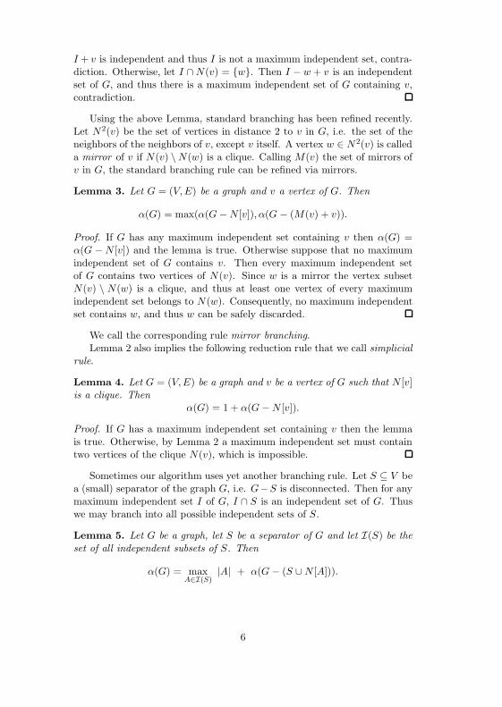
I + v is independent and thus I is not a maximum independent set, contra-diction. Otherwise, let I ∩N(v) = w. Then I − w + v is an independentset of G, and thus there is a maximum independent set of G containing v,contradiction.

Using the above Lemma, standard branching has been refined recently.Let N2(v) be the set of vertices in distance 2 to v in G, i.e. the set of theneighbors of the neighbors of v, except v itself. A vertex w ∈ N2(v) is calleda mirror of v if N(v) \N(w) is a clique. Calling M(v) the set of mirrors ofv in G, the standard branching rule can be refined via mirrors.

Lemma 3. Let G = (V,E) be a graph and v a vertex of G. Then

α(G) = max(α(G−N [v]), α(G − (M(v) + v)).

Proof. If G has any maximum independent set containing v then α(G) =α(G −N [v]) and the lemma is true. Otherwise suppose that no maximumindependent set of G contains v. Then every maximum independent setof G contains two vertices of N(v). Since w is a mirror the vertex subsetN(v) \ N(w) is a clique, and thus at least one vertex of every maximumindependent set belongs to N(w). Consequently, no maximum independentset contains w, and thus w can be safely discarded.

We call the corresponding rule mirror branching.Lemma 2 also implies the following reduction rule that we call simplicial

rule.

Lemma 4. Let G = (V,E) be a graph and v be a vertex of G such that N [v]is a clique. Then

α(G) = 1 + α(G−N [v]).

Proof. If G has a maximum independent set containing v then the lemmais true. Otherwise, by Lemma 2 a maximum independent set must containtwo vertices of the clique N(v), which is impossible.

Sometimes our algorithm uses yet another branching rule. Let S ⊆ V bea (small) separator of the graph G, i.e. G−S is disconnected. Then for anymaximum independent set I of G, I ∩ S is an independent set of G. Thuswe may branch into all possible independent sets of S.

Lemma 5. Let G be a graph, let S be a separator of G and let I(S) be theset of all independent subsets of S. Then

α(G) = maxA∈I(S)

|A| + α(G − (S ∪N [A])).

6

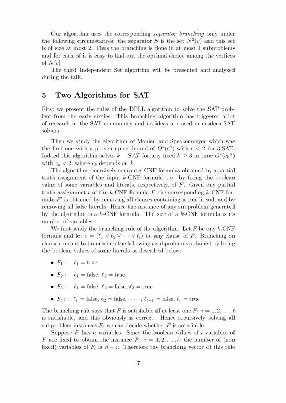
Our algorithm uses the corresponding separator branching only underthe following circumstances: the separator S is the set N2(v) and this setis of size at most 2. Thus the branching is done in at most 4 subproblemsand for each of it is easy to find out the optimal choice among the verticesof N [v].

The third Independent Set algorithm will be presented and analyzedduring the talk.

5 Two Algorithms for SAT

First we present the rules of the DPLL algorithm to solve the SAT prob-lem from the early sixties. This branching algorithm has triggered a lotof research in the SAT community and its ideas are used in modern SATsolvers.

Then we study the algorithm of Monien and Speckenmeyer which wasthe first one with a proven upper bound of O∗(cn) with c < 2 for 3-SAT.Indeed this algorithm solves k − SAT for any fixed k ≥ 3 in time O∗(ck

n)with ck < 2, where ck depends on k.

The algorithm recursively computes CNF formulas obtained by a partialtruth assignment of the input k-CNF formula, i.e. by fixing the booleanvalue of some variables and literals, respectively, of F . Given any partialtruth assignment t of the k-CNF formula F the corresponding k-CNF for-mula F ′ is obtained by removing all clauses containing a true literal, and byremoving all false literals. Hence the instance of any subproblem generatedby the algorithm is a k-CNF formula. The size of a k-CNF formula is itsnumber of variables.

We first study the branching rule of the algorithm. Let F be any k-CNFformula and let c = (1 ∨ 2 ∨ · · · ∨ t) be any clause of F . Branching onclause c means to branch into the following t subproblems obtained by fixingthe boolean values of some literals as described below:

• F1 : 1 = true

• F2 : 1 = false, 2 = true

• F3 : 1 = false, 2 = false, 3 = true

• Ft : 1 = false, 2 = false, · · · , t−1 = false, t = true

The branching rule says that F is satisfiable iff at least one Fi, i = 1, 2, . . . , tis satisfiable, and this obviously is correct. Hence recursively solving allsubproblem instances Fi we can decide whether F is satisfiable.

Suppose F has n variables. Since the boolean values of i variables ofF are fixed to obtain the instance Fi, i = 1, 2, . . . , t, the number of (nonfixed) variables of Fi is n − i. Therefore the branching vector of this rule

7

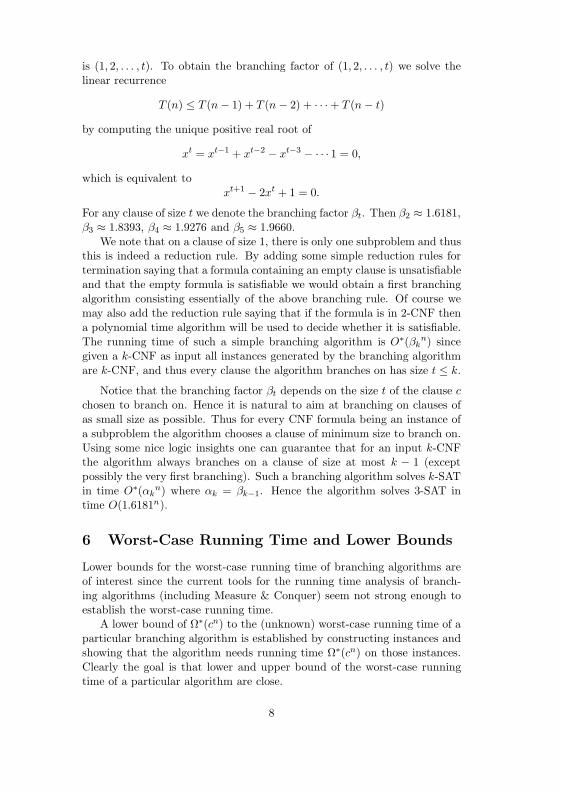
is (1, 2, . . . , t). To obtain the branching factor of (1, 2, . . . , t) we solve thelinear recurrence

T (n) ≤ T (n− 1) + T (n− 2) + · · ·+ T (n− t)

by computing the unique positive real root of

xt = xt−1 + xt−2 − xt−3 − · · · 1 = 0,

which is equivalent toxt+1 − 2xt + 1 = 0.

For any clause of size t we denote the branching factor βt. Then β2 ≈ 1.6181,β3 ≈ 1.8393, β4 ≈ 1.9276 and β5 ≈ 1.9660.

We note that on a clause of size 1, there is only one subproblem and thusthis is indeed a reduction rule. By adding some simple reduction rules fortermination saying that a formula containing an empty clause is unsatisfiableand that the empty formula is satisfiable we would obtain a first branchingalgorithm consisting essentially of the above branching rule. Of course wemay also add the reduction rule saying that if the formula is in 2-CNF thena polynomial time algorithm will be used to decide whether it is satisfiable.The running time of such a simple branching algorithm is O∗(βk

n) sincegiven a k-CNF as input all instances generated by the branching algorithmare k-CNF, and thus every clause the algorithm branches on has size t ≤ k.

Notice that the branching factor βt depends on the size t of the clause cchosen to branch on. Hence it is natural to aim at branching on clauses ofas small size as possible. Thus for every CNF formula being an instance ofa subproblem the algorithm chooses a clause of minimum size to branch on.Using some nice logic insights one can guarantee that for an input k-CNFthe algorithm always branches on a clause of size at most k − 1 (exceptpossibly the very first branching). Such a branching algorithm solves k-SATin time O∗(αk

n) where αk = βk−1. Hence the algorithm solves 3-SAT intime O(1.6181n).

6 Worst-Case Running Time and Lower Bounds

Lower bounds for the worst-case running time of branching algorithms areof interest since the current tools for the running time analysis of branch-ing algorithms (including Measure & Conquer) seem not strong enough toestablish the worst-case running time.

A lower bound of Ω∗(cn) to the (unknown) worst-case running time of aparticular branching algorithm is established by constructing instances andshowing that the algorithm needs running time Ω∗(cn) on those instances.Clearly the goal is that lower and upper bound of the worst-case runningtime of a particular algorithm are close.

8

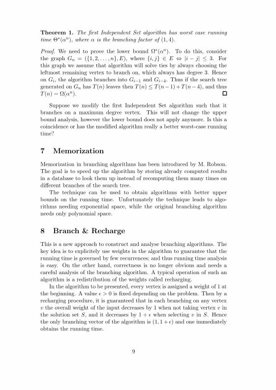
Theorem 1. The first Independent Set algorithm has worst case runningtime Θ∗(αn), where α is the branching factor of (1, 4).

Proof. We need to prove the lower bound Ω∗(αn). To do this, considerthe graph Gn = (1, 2, . . . , n, E), where i, j ∈ E ⇔ |i − j| ≤ 3. Forthis graph we assume that algorithm will solve ties by always choosing theleftmost remaining vertex to branch on, which always has degree 3. Henceon Gi, the algorithm branches into Gi−1 and Gi−4. Thus if the search treegenerated on Gn has T (n) leaves then T (n) ≤ T (n−1)+T (n−4), and thusT (n) = Ω(αn).

Suppose we modify the first Independent Set algorithm such that itbranches on a maximum degree vertex. This will not change the upperbound analysis, however the lower bound does not apply anymore. Is this acoincidence or has the modified algorithm really a better worst-case runningtime?

7 Memorization

Memorization in branching algorithms has been introduced by M. Robson.The goal is to speed up the algorithm by storing already computed resultsin a database to look them up instead of recomputing them many times ondifferent branches of the search tree.

The technique can be used to obtain algorithms with better upperbounds on the running time. Unfortunately the technique leads to algo-rithms needing exponential space, while the original branching algorithmneeds only polynomial space.

8 Branch & Recharge

This is a new approach to construct and analyse branching algorithms. Thekey idea is to explicitely use weights in the algorithm to guarantee that therunning time is governed by few recurrences; and thus running time analysisis easy. On the other hand, correctness is no longer obvious and needs acareful analysis of the branching algorithm. A typical operation of such analgorithm is a redistribution of the weights called recharging.

In the algorithm to be presented, every vertex is assigned a weight of 1 atthe beginning. A value ε > 0 is fixed depending on the problem. Then by arecharging procedure, it is guaranteed that in each branching on any vertexv the overall weight of the input decreases by 1 when not taking vertex v inthe solution set S, and it decreases by 1 + ε when selecting v in S. Hencethe only branching vector of the algorithm is (1, 1+ ε) and one immediatelyobtains the running time.

9

Exercices

The exercices are ordered from easy ones to research problems.

1. The HAMILTONIAN CIRCUIT problem can be solved in time O∗(2n) viadynamic programming or inclusion-exclusion. Construct a O∗(3m/3) branch-ing algorithm deciding whether a graph has a hamiltonian circuit, where mis the number of edges.

2. Let G = (V, E) be a bicolored graph, i.e. its vertices are either red or blue.Construct and analyze branching algorithms that for input G, k1, k2 decidewhether the bicolored graph G has an independent set I with k1 red and k2

blue vertices. What is the best running time you can establish?

3. Construct a branching algorithm for the 3-COLORING problem, i.e. forgiven graph G it decides whether G is 3-colorable. The running time shouldbe O∗(3n/3) or even O∗(cn) for some c < 1.4.

4. Construct a branching algorithm for the DOMINATING SET problem ongraphs of maximum degree 3.

5. Is the following statement true for all graphs G. If w is a mirror of v andthere is a maximum independent set of G not containing v, then there is amaximum independent set containing neither v nor w.

6. Modify the first IS algorithm such that it always branches on a maximumdegree vertex. Provide a lower bound. What is the worst-case running timeof this algorithm?

7. Construct a O∗(1.49n) branching algorithm to solve 3-SAT.

References

[1] T.H. Cormen, C.E. Leiserson, R.L. Rivest, C. Stein, Introduction to Algo-rithms, MIT Press, 2001.

[2] J. Kleinberg, E. Tardos, Algorithm Design, Addison-Wesley, 2005.

[3] R.L. Graham, D.E. Knuth, O. Patashnik Concrete Mathematics, Addison-Wesley, 1989.

[4] R. Beigel and D. Eppstein. 3-coloring in time O(1.3289n). Journal of Algo-rithms 54:168–204, 2005.

[5] M. Davis, H. Putnam. A computing procedure for quantification theory. J.ACM 7:201–215, 1960.

[6] D. Eppstein. The traveling salesman problem for cubic graphs. In Workshopon Algorithms and Data Structures (WADS), pages 307–318, 2003.

[7] F. V. Fomin, S. Gaspers, and A. V. Pyatkin. Finding a minimum feedback ver-tex set in time O(1.7548n), in Proceedings of the 2nd International Workshopon Parameterized and Exact Computation (IWPEC 2006), Springer LNCSvol. 4169, pp. 184–191.

10

[8] F. V. Fomin, P. Golovach, D. Kratsch, J. Kratochvil and M. Liedloff. Branchand Recharge: Exact algorithms for generalized domination. Proceedings ofWADS 2007, Springer, 2007, LNCS 4619, pp. 508–519.

[9] F. V. Fomin, F. Grandoni, D. Kratsch. Some new techniques in design andanalysis of exact (exponential) algorithms. Bulletin of the EATCS 87:47–77,2005.

[10] F. V. Fomin, F. Grandoni, D. Kratsch. Measure and Conquer: A SimpleO(20.288 n) Independent Set Algorithm. Proceedings of SODA 2006, ACM andSIAM, 2006, pp. 508–519.

[11] K. Iwama. Worst-case upper bounds for k-SAT. Bulletin of the EATCS 82:61–71, 2004.

[12] K. Iwama and S. Tamaki. Improved upper bounds for 3-SAT. Proceedings ofSODA 2004, ACM and SIAM, 2004, p. 328.

[13] B. Monien, E. Speckenmeyer. Solving satisfiability in less than 2n steps. Dis-crete Appl. Math. 10: 287–295, 1985.

[14] I. Razgon. Exact computation of maximum induced forest. Proceedings of the10th Scandinavian Workshop on Algorithm Theory (SWAT 2006). SpringerLNCS vol. 4059, p. 160-171.

[15] J. M. Robson. Algorithms for maximum independent sets. Journal of Algo-rithms 7(3):425–440, 1986.

[16] R. Tarjan and A. Trojanowski. Finding a maximum independent set. SIAMJournal on Computing, 6(3):537–546, 1977.

[17] G. J. Woeginger. Exact algorithms for NP-hard problems: A survey. Combi-natorial Optimization – Eureka, You Shrink, Springer LNCS vol. 2570, 2003,pp. 185–207.

[18] G. J. Woeginger. Space and time complexity of exact algorithms: Someopen problems. Proceedings of the 1st International Workshop on Param-eterized and Exact Computation (IWPEC 2004), Springer LNCS vol. 3162,2004, pp. 281–290.

[19] G. J. Woeginger. Open problems around exact algorithms. Discrete AppliedMathematics, 156:397–405, 2008.

11

Daniel Marx

FPT algorithmic techniques

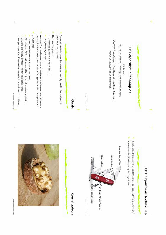
FP

Talg

orith

mic

techn

iqu

es

DánielM

arx

BudapestU

niversityofTechnology

andE

conomics,H

ungary

AG

AP

E’09

Spring

Schoolon

Fixed

Param

eterand

ExactA

lgorithms

May

25-26,2009,Lozari,Corsica

(France)

FP

Talgorithm

ictechniques

–p.1/97

FP

Talg

orith

mic

techn

iqu

es

Significantadvances

inthe

past20years

orso

(especiallyin

recentyears).

Pow

erfultoolboxfor

designingF

PT

algorithms:Iterative

com

pressio

nTreew

idth

Bo

un

ded

Search

Tree

Grap

hM

ino

rsT

heo

remC

olo

rco

din

g

Kern

elization

FP

Talgorithm

ictechniques

–p.2/97

Go

als

Dem

onstratetechniques

thatwere

successfullyused

inthe

analysisof

parameterized

problems.

There

aretw

ogoals:

Determ

inequickly

ifaproblem

isF

PT.

Design

fastalgorithms.

Warning:

The

resultspresented

forparticular

problems

arenotnecessarily

thebestknow

nresults

orthe

mostusefulapproaches

forthese

problems.

Conventions:

Unless

notedotherw

ise,k

isthe

parameter.

O∗

notation:O∗(f

(k))

means

O(f

(k)·

nc)

forsom

econstant

c.

Citations

arem

ostlyom

itted(only

forclassicalresults).

We

glossover

thedifference

between

decisionand

searchproblem

s.

FP

Talgorithm

ictechniques

–p.3/97

Kern

elization

FP

Talgorithm

ictechniques

–p.4/97

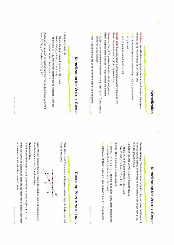
Kern

elization

Defi

nitio

n:

Kern

elization

isa

polynomial-tim

etransform

ationthatm

apsan

instance(I

,k)

toan

instance(I′,

k′)

suchthat

(I,k)

isa

yes-instanceifand

onlyif(I′,

k′)

isa

yes-instance,

k′≤

k,and

|I′|≤

f(k

)for

some

functionf(k′).

Sim

ple

fact:Ifa

problemhas

akernelization

algorithm,then

itisF

PT.

Pro

of:

Solve

theinstance

(I′,

k′)

bybrute

force.

Co

nverse:E

veryF

PT

problemhas

akernelization

algorithm.

Pro

of:

Suppose

thereis

anf(k

)nc

algorithmfor

theproblem

.

Iff(k

)≤n

,thensolve

theinstance

intim

ef(k

)nc≤

nc+

1,andoutputa

trivialyes-or

no-instance.

Ifn

<f(k

),thenw

eare

done:a

kernelofsizef(k

)is

obtained.F

PT

algorithmic

techniques–

p.5/97

Kern

elization

for

VE

RT

EX

CO

VE

R

Gen

eralstrategy:

We

devisea

listofreductionrules,and

showthatifnone

of

therules

canbe

appliedand

thesize

oftheinstance

isstilllarger

thanf(k

),then

theansw

eris

trivial.

Reduction

rulesfor

VE

RT

EX

CO

VE

Rinstance

(G,k):

Ru

le1:

Ifv

isan

isolatedvertex⇒

(G\

v,k)

Ru

le2:

Ifd(v

)>

k⇒

(G\

v,k−

1)

IfneitherR

ule1

norR

ule2

canbe

applied:

If|V(G

)|>

k(k

+1)⇒

There

isno

solution(every

vertexshould

bethe

neighborofatleastone

vertexofthe

cover).

Otherw

ise,|V(G

)|≤k(k

+1)

andw

ehave

ak(k

+1)

vertexkernel.

FP

Talgorithm

ictechniques

–p.6/97

Kern

elization

for

VE

RT

EX

CO

VE

R

Letusadd

athird

rule:

Ru

le1:

Ifv

isan

isolatedvertex⇒

(G\

v,k)

Ru

le2:

Ifd(v

)>

k⇒

(G\

v,k−

1)

Ru

le3:

Ifd(v

)=

1,then

we

canassum

ethatits

neighboru

isin

the

solution⇒(G\

(u∪

v),

k−

1).

Ifnoneofthe

rulescan

beapplied,then

everyvertex

hasdegree

atleast2

.N

ow|E

(G)|≤

k2

implies|V

(G)|≤

k2.

FP

Talgorithm

ictechniques

–p.7/97

CO

VE

RIN

GP

OIN

TS

WIT

HL

INE

S

Task:G

ivena

setP

ofn

pointsin

theplane

andan

integerk

,findk

linesthat

coverallthe

points.

No

te:W

ecan

assume

thateveryline

ofthesolution

coversatleast2

points,

thusthere

areatm

ostn

2candidate

lines.

Red

uctio

nR

ule:

Ifacandidate

linecovers

aset

Sofm

orethan

kpoints⇒

(P\

S,k−

1).

Ifthisrule

cannotbeapplied

andthere

arestillm

orethan

k2

points,thenthere

isno

solution⇒K

ernelwith

atmost

k2

points.F

PT

algorithmic

techniques–

p.8/97

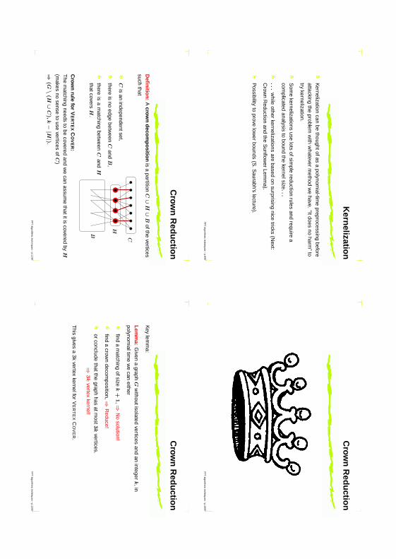
Kern

elization

Kernelization

canbe

thoughtofasa

polynomial-tim

epreprocessing

before

attackingthe

problemw

ithw

hateverm

ethodw

ehave.

“Itdoesno

harm”

totry

kernelization.

Som

ekernelizations

uselots

ofsimple

reductionrules

andrequire

a

complicated

analysisto

boundthe

kernelsize...

...

while

otherkernelizations

arebased

onsurprising

nicetricks

(Next:

Crow

nR

eductionand

theS

unflower

Lemm

a).

Possibility

toprove

lower

bounds(S

.Saurabh’s

lecture).

FP

Talgorithm

ictechniques

–p.9/97

Crow

nR

edu

ction

FP

Talgorithm

ictechniques

–p.10/97

Crow

nR

edu

ction

Defi

nitio

n:

Acro

wn

deco

mp

ositio

nis

apartition

C∪

H∪

Bofthe

vertices

suchthat

Cis

anindependentset,

thereis

noedge

between

Cand

B,

thereis

am

atchingbetw

eenC

andH

thatcoversH

.B

C

H

Cro

wn

rule

for

VE

RT

EX

CO

VE

R:

The

matching

needsto

becovered

andw

ecan

assume

thatitiscovered

byH

(makes

nosense

touse

verticesof

C)

⇒(G\

(H∪

C),

k−|H|).

FP

Talgorithm

ictechniques

–p.11/97

Crow

nR

edu

ction

Key

lemm

a:

Lem

ma:

Given

agraph

Gw

ithoutisolatedvertices

andan

integerk

,in

polynomialtim

ew

ecan

either

finda

matching

ofsizek

+1

,⇒N

osolution!

finda

crown

decomposition,⇒

Reduce!

orconclude

thatthegraph

hasatm

ost3k

vertices.⇒

3k

vertexkernel!

This

givesa

3kvertex

kernelforV

ER

TE

XC

OV

ER

.

FP

Talgorithm

ictechniques

–p.12/97

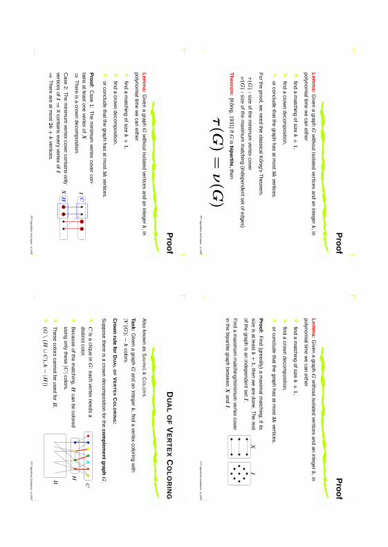
Pro

of

Lem

ma:

Given

agraph

Gw

ithoutisolatedvertices

andan

integerk

,in

polynomialtim

ew

ecan

either

finda

matching

ofsizek

+1

,

finda

crown

decomposition,

orconclude

thatthegraph

hasatm

ost3k

vertices.

For

theproof,w

eneed

theclassicalK

onig’sT

heorem.

τ(G

):

sizeofthe

minim

umvertex

coverν(G

):

sizeofthe

maxim

umm

atching(independentsetofedges)

Th

eorem

:[K

onig,1931]IfG

isb

ipartite,then

τ(G

)=

ν(G

)F

PT

algorithmic

techniques–

p.13/97

Pro

of

Lem

ma:

Given

agraph

Gw

ithoutisolatedvertices

andan

integerk

,in

polynomialtim

ew

ecan

either

finda

matching

ofsizek

+1

,

finda

crown

decomposition,

orconclude

thatthegraph

hasatm

ost3k

vertices.

Pro

of:

Find

(greedily)a

maxim

almatching;

ifits

sizeis

atleastk

+1

,thenw

eare

done.T

herest

ofthegraph

isan

independentsetI

.

Find

am

aximum

matching/m

inimum

vertexcover

inthe

bipartitegraph

between

Xand

I.

IX

FP

Talgorithm

ictechniques

–p.14/97

Pro

of

Lem

ma:

Given

agraph

Gw

ithoutisolatedvertices

andan

integerk

,in

polynomialtim

ew

ecan

either

finda

matching

ofsizek

+1

,

finda

crown

decomposition,

orconclude

thatthegraph

hasatm

ost3k

vertices.

Pro

of:

Case

1:T

hem

inimum

vertexcover

con-

tainsatleastone

vertexof

X

⇒T

hereis

acrow

ndecom

position.

Case

2:T

hem

inimum

vertexcover

containsonly

verticesof

I⇒Itcontains

everyvertex

ofI

⇒T

hereare

atmost

2k

+k

vertices.

CHX I

FP

Talgorithm

ictechniques

–p.14/97

DU

AL

OF

VE

RT

EX

CO

LO

RIN

G

Also

known

asS

AV

ING

kC

OL

OR

S.

Task:G

ivena

graphG

andan

integerk

,finda

vertexcoloring

with

|V(G

)|−k

colors.

Cro

wn

rule

for

DU

AL

OF

VE

RT

EX

CO

LO

RIN

G:

Suppose

thereis

acrow

ndecom

positionfor

theco

mp

lemen

tg

raph

G.

Cis

aclique

inG

:each

vertexneeds

a

distinctcolor.

Because

ofthem

atching,H

canbe

colored

usingonly

these|C|

colors.

These

colorscannotbe

usedfor

B.

(G\

(H∪

C),

k−|H|)

B

C

H

FP

Talgorithm

ictechniques

–p.15/97

Crow

nR

edu

ction

for

DU

AL

OF

VE

RT

EX

CO

LO

RIN

G

Use

thekey

lemm

afor

thecom

plement

Gof

G:

Lem

ma:

Given

agraph

Gw

ithoutisolatedvertices

andan

integerk

,inpolynom

ialtime

we

caneither

finda

matching

ofsizek

+1

,⇒Y

ES

:we

cansave

kcolors!

finda

crown

decomposition,⇒

Reduce!

orconclude

thatthegraph

hasatm

ost3k

vertices.

⇒3k

vertexkernel!

This

givesa

3kvertex

kernelforD

UA

LO

FV

ER

TE

XC

OL

OR

ING

.

FP

Talgorithm

ictechniques

–p.16/97

Su

nfl

ower

Lem

ma

FP

Talgorithm

ictechniques

–p.17/97

Su

nfl

ower

lemm

a

Defi

nitio

n:

Sets

S1 ,

S2 ,

...,

Sk

forma

sun

flo

wer

ifthesets

Si \

(S1 ∩

S2 ∩

···∩S

k)

aredisjoint.

petalscenter

Lem

ma:

[Erdos

andR

ado,1960]Ifthesize

ofasetsystem

isgreater

than

(p−

1)

d·d!

anditcontains

onlysets

ofsizeatm

ostd

,thenthe

systemcontains

asunflow

erw

ithp

petals.F

urthermore,in

thiscase

sucha

sunflower

canbe

foundin

polynomialtim

e.

FP

Talgorithm

ictechniques

–p.18/97

Su

nfl

owers

and

d-H

ITT

ING

SE

T

d-H

ITT

ING

SE

T:G

ivena

collectionSofsets

ofsizeatm

ostd

andan

integer

k,find

aset

Sof

kelem

entsthatintersects

everysetofS

.

petalscenter

Red

uctio

nR

ule:

Ifk

+1

setsform

asunflow

er,thenrem

ovethese

setsfrom

Sand

addthe

centerC

toS(S

doesnothitone

ofthepetals,thus

ithasto

hit

thecenter).

Iftherule

cannotbeapplied,then

thereare

atmost

kd·

d!=

O(k

d)

sets.

FP

Talgorithm

ictechniques

–p.19/97

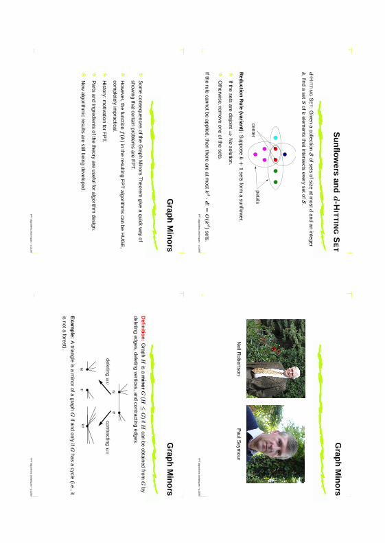
Su

nfl

owers

and

d-H

ITT

ING

SE

T

d-H

ITT

ING

SE

T:G

ivena

collectionSofsets

ofsizeatm

ostd

andan

integer

k,find

aset

Sof

kelem

entsthatintersects

everysetofS

.

petalscenter

Red

uctio

nR

ule

(variant):

Suppose

k+

1sets

forma

sunflower.

Ifthesets

aredisjoint⇒

No

solution.

Otherw

ise,remove

oneofthe

sets.

Iftherule

cannotbeapplied,then

thereare

atmost

kd·

d!=

O(k

d)

sets.F

PT

algorithmic

techniques–

p.19/97

Grap

hM

ino

rs

NeilR

obertsonP

aulSeym

ourFP

Talgorithm

ictechniques

–p.20/97

Grap

hM

ino

rs

Som

econsequences

oftheG

raphM

inorsT

heoremgive

aquick

way

of

showing

thatcertainproblem

sare

FP

T.

How

ever,thefunction

f(k

)in

theresulting

FP

Talgorithm

scan

beH

UG

E,

completely

impractical.

History:

motivation

forF

PT.

Parts

andingredients

ofthetheory

areusefulfor

algorithmdesign.

New

algorithmic

resultsare

stillbeingdeveloped.

FP

Talgorithm

ictechniques

–p.21/97

Grap

hM

ino

rs

Defi

nitio

n:

Graph

His

am

ino

rG

(H≤

G)

ifH

canbe

obtainedfrom

Gby

deletingedges,deleting

vertices,andcontracting

edges.

deletingu

v

w

u

u

v

v

contractingu

v

Exam

ple:

Atriangle

isa

minor

ofagraph

Gifand

onlyif

Ghas

acycle

(i.e.,it

isnota

forest).

FP

Talgorithm

ictechniques

–p.22/97

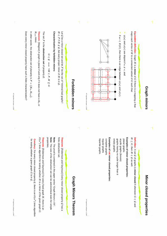
Grap

hm

ino

rs

Eq

uivalen

td

efin

ition

:G

raphH

isa

min

or

ofG

ifthereis

am

appingφ

that

maps

eachvertex

ofH

toa

connectedsubsetof

Gsuch

that

φ(u

)and

φ(v

)are

disjointifu6=

v,and

ifu

v∈

E(G

),thenthere

isan

edgebetw

eenφ(u

)and

φ(v

).

2

76

54

31

77

46

5

7 6 32

14

5

675

FP

Talgorithm

ictechniques

–p.23/97

Min

or

closed

pro

perties

Defi

nitio

n:

AsetG

ofgraphsis

min

or

closed

ifwhenever

G∈G

and

H≤

G,then

H∈G

asw

ell.

Exam

ples

of

min

or

closed

pro

perties:

planargraphs

acyclicgraphs

(forests)

graphshaving

nocycle

longerthan

k

empty

graphs

Exam

ples

of

no

tm

ino

rclo

sedp

rop

erties:com

pletegraphs

regulargraphs

bipartitegraphs

FP

Talgorithm

ictechniques

–p.24/97

Fo

rbid

den

min

ors

LetGbe

am

inorclosed

setandletF

bethe

setof“minim

albadgraphs”:

H∈F

ifH6∈G

,buteveryproper

minor

ofH

isinG

.

Ch

aracterization

byfo

rbid

den

min

ors:

G∈G⇐⇒

∀H∈F

,H6≤

G

The

setFis

theo

bstru

ction

setofpropertyG

.

Th

eorem

:[W

agner]Agraph

isplanar

ifandonly

ifitdoesnothave

aK

5or

K3

,3m

inor.

Inother

words:

theobstruction

setofplanarityisF

=K

5,K

3,3

.

Does

everym

inorclosed

propertyhave

sucha

finitecharacterization?

FP

Talgorithm

ictechniques

–p.25/97

Grap

hM

ino

rsT

heo

rem

Th

eorem

:[R

obertsonand

Seym

our]Every

minor

closedpropertyG

hasa

finiteobstruction

set.

No

te:T

heproofis

containedin

thepaper

series“G

raphM

inorsI–X

X”.

No

te:T

hesize

oftheobstruction

setcanbe

astronomicaleven

forsim

pleproperties.

Th

eorem

:[R

obertsonand

Seym

our]For

everyfixed

graphH

,thereis

an

O(n

3)

time

algorithmfor

testingw

hetherH

isa

minor

ofthegiven

graphG

.

Co

rollary:

Forevery

minorclosed

propertyG,there

isan

O(n

3)

time

algorithmfor

testingw

hethera

givengraph

Gis

inG.

FP

Talgorithm

ictechniques

–p.26/97

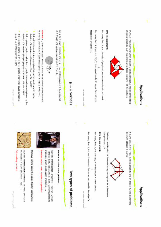
Ap

plicatio

ns

PL

AN

AR

FA

CE

CO

VE

R:

Given

agraph

Gand

aninteger

k,find

anem

bedding

ofplanargraph

Gsuch

thatthereare

kfaces

thatcoverallthe

vertices.

On

elin

earg

um

ent:

For

everyfixed

k,the

classGk

ofgraphsofyes-instances

ism

inorclosed.

⇓F

orevery

fixedk

,thereis

aO

(n3)

time

algorithmfor

PL

AN

AR

FA

CE

CO

VE

R.

No

te:non-uniform

FP

T.

FP

Talgorithm

ictechniques

–p.27/97

Ap

plicatio

ns

k-L

EA

FS

PA

NN

ING

TR

EE

:G

ivena

graphG

andan

integerk

,finda

spanning

treew

ithat

leastk

leaves.

Technicalmodification:

Isthere

sucha

spanningtree

foratleastone

componentof

G?

On

elin

earg

um

ent:

For

everyfixed

k,the

classGk

ofno-instancesis

minor

closed.

⇓F

orevery

fixedk

,k

-LE

AF

SP

AN

NIN

GT

RE

Ecan

besolved

intim

eO

(n3).

FP

Talgorithm

ictechniques

–p.28/97

G+

kvertices

LetGbe

agraph

property,andletG

+kv

containgraph

Gifthere

isa

set

S⊆

V(G

)of

kvertices

suchthat

G\

S∈G

.

S

Lem

ma:

IfGis

minor

closed,thenG+

kv

ism

inorclosed

forevery

fixedk

.⇒

Finding

thesm

allestk

suchthata

givengraph

isinG

+kv

isF

PT.

IfG=

forests⇒G

+kv

=graphs

thatcanbe

made

acyclicby

thedeletion

ofk

vertices⇒F

EE

DB

AC

KV

ER

TE

XS

ET

isF

PT.

IfG=

planargraphs⇒

G+

kv

=graphs

thatcanbe

made

planarby

the

deletionof

kvertices

(k-apex

graphs)⇒k

-AP

EX

GR

AP

His

FP

T.

IfG=

empty

graphs⇒G

+kv

=graphs

with

vertexcover

number

atm

ostk⇒

VE

RT

EX

CO

VE

Ris

FP

T.F

PT

algorithmic

techniques–

p.29/97

Two

types

of

pro

blem

s

We

have

toso

lveso

me

pro

blem

s.

Typicallym

inim

ization

problems:

VE

RT

EX

CO

VE

R,

HIT

TIN

GS

ET,

DO

MIN

AT

ING

SE

T,covering/stabbing

problems,graph

modification

problems,

...

Bounded

searchtrees,iterative

compression

We

have

tofi

nd

som

ethin

gn

iceh

idd

enso

mew

here.

Typicallym

aximizatio

nproblem

s:k

-PA

TH

,D

ISJO

INT

TR

IAN

GL

ES,

k-L

EA

FS

PA

NN

ING

TR

EE,

...

Color

coding,matroids

FP

Talgorithm

ictechniques

–p.30/97

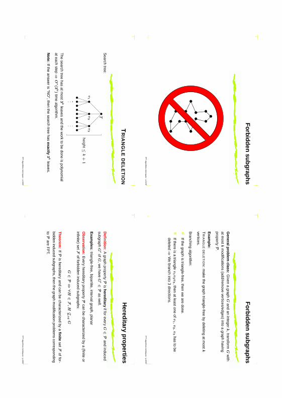
Fo

rbid

den

sub

grap

hs

FP

Talgorithm

ictechniques

–p.31/97

Fo

rbid

den

sub

grap

hs

Gen

eralpro

blem

class:G

ivena

graphG

andan

integerk

,transformG

with

atmost

km

odifications(add/rem

ovevertices/edges)

intoa

graphhaving

propertyP.

Exam

ple:

TR

IAN

GL

ED

EL

ET

ION

:m

akethe

graphtriangle-free

bydeleting

atmost

k

vertices.

Branching

algorithm:

Ifthegraph

istriangle-free,then

we

aredone.

Ifthereis

atriangle

v1v2v3 ,then

atleastoneof

v1 ,

v2 ,

v3

hasto

be

deleted⇒W

ebranch

into3

directions.

FP

Talgorithm

ictechniques

–p.32/97

TR

IAN

GL

ED

EL

ET

ION

Search

tree:

height≤k

+1

v2

T

v1

v3

The

searchtree

hasatm

ost3

kleaves

andthe

work

tobe

doneis

polynomial

ateachstep⇒

O∗(3

k)

time

algorithm.

No

te:Ifthe

answer

is“N

O”,then

thesearch

treehas

exactly3

kleaves.

FP

Talgorithm

ictechniques

–p.33/97

Hered

itaryp

rop

erties

Defi

nitio

n:

Agraph

propertyPis

hered

itaryiffor

everyG∈P

andinduced

subgraphG′

ofG

,we

haveG′∈

Pas

well.

Exam

ples:

triangle-free,bipartite,intervalgraph,planar

Ob

servation

:E

veryhereditary

propertyPcan

becharacterized

bya

(finiteor

infinite)setF

offorbiddeninduced

subgraphs:

G∈P⇔∀H∈F

,H6⊆

indG

Th

eorem

:IfP

ishereditary

andcan

becharacterized

bya

fin

itesetF

offor-

biddeninduced

subgraphs,thenthe

graphm

odificationproblem

scorresponding

toPare

FP

T.

FP

Talgorithm

ictechniques

–p.34/97

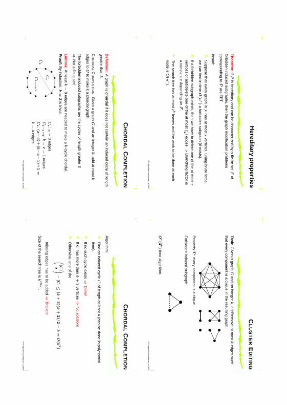
Hered

itaryp

rop

erties

Th

eorem

:IfP

ishereditary

andcan

becharacterized

bya

fin

itesetF

of

forbiddeninduced

subgraphs,thenthe

graphm

odificationproblem

scorresponding

toPare

FP

T.

Pro

of:

Suppose

thateverygraph

inFhas

atmost

rvertices.

Using

bruteforce,

we

canfind

intim

eO

(nr)

aforbidden

subgraph(ifexists).

Ifaforbidden

subgraphexists,then

we

haveto

deleteone

oftheatm

ostr

verticesor

add/deleteone

oftheatm

ost (r2 )

edges⇒B

ranchingfactor

is

aconstant

cdepending

onF.

The

searchtree

hasatm

ostc

kleaves

andthe

work

tobe

doneateach

nodeis

O(n

r).

FP

Talgorithm

ictechniques

–p.35/97

CL

US

TE

RE

DIT

ING

Task:G

ivena

graphG

andan

integerk

,add/remove

atmost

kedges

such

thateverycom

ponentisa

cliquein

theresulting

graph.

PropertyP

:every

componentis

aclique.

Forbidden

inducedsubgraph:

O∗(3

k)

time

algorithm.

FP

Talgorithm

ictechniques

–p.36/97

CH

OR

DA

LC

OM

PL

ET

ION

Defi

nitio

n:

Agraph

isch

ord

alifitdoesnotcontain

aninduced

cycleoflength

greaterthan

3.

CH

OR

DA

LC

OM

PL

ET

ION

:G

ivena

graphG

andan

integerk

,addatm

ostk

edgesto

Gto

make

itachordalgraph.

The

forbiddeninduced

subgraphsare

thecycles

oflengthgreater

3

⇒N

otafinite

set!

Lem

ma:

Atleast

k−

3edges

areneeded

tom

akea

k-cycle

chordal.

Pro

of:

By

induction.k

=3

istrivial.

Ck

Ck−

x+

2

Cx

Cx

:x−

3edges

Ck−

x+

2 :k−

x−

1edges

Ck :

(x−3)+

(k−x−

1)+

1=

k−

3edges

FP

Talgorithm

ictechniques

–p.37/97

CH

OR

DA

LC

OM

PL

ET

ION

Algorithm

:

Find

aninduced

cycleC

oflengthatleast4

(canbe

donein

polynomial

time).

Ifnosuch

cycleexists⇒

Done!

IfC

hasm

orethan

k+

3vertices⇒

No

solution!

Otherw

ise,oneofthe

(|C|2 )−|C|≤

(k+

3)(k

+2)/

2−k

=O

(k2)

missing

edgeshas

tobe

added ⇒B

ranch!

Size

ofthesearch

treeis

kO

(k).

FP

Talgorithm

ictechniques

–p.38/97

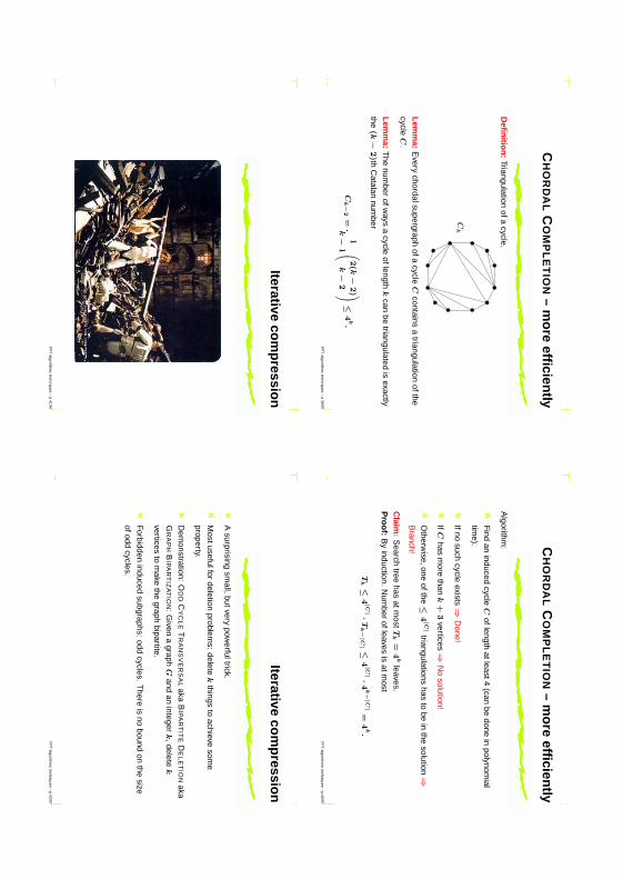
CH

OR

DA

LC

OM

PL

ET

ION

–m

ore

efficien

tly

Defi

nitio

n:

Triangulationofa

cycle.

Ck

Lem

ma:

Every

chordalsupergraphofa

cycleC

containsa

triangulationofthe

cycleC

.

Lem

ma:

The

number

ofways

acycle

oflengthk

canbe

triangulatedis

exactly

the(k−

2)th

Catalan

number

Ck−

2=

1

k−

1 (2(k−

2)

k−

2 )≤

4k.

FP

Talgorithm

ictechniques

–p.39/97

CH

OR

DA

LC

OM

PL

ET

ION

–m

ore

efficien

tly

Algorithm

:

Find

aninduced

cycleC

oflengthatleast4

(canbe

donein

polynomial

time).

Ifnosuch

cycleexists⇒

Done!

IfC

hasm

orethan

k+

3vertices⇒

No

solution!

Otherw

ise,oneofthe≤

4|C|

triangulationshas

tobe

inthe

solution⇒B

ranch!

Claim

:S

earchtree

hasatm

ostT

k=

4k

leaves.

Pro

of:

By

induction.N

umber

ofleavesis

atmost

Tk≤

4|C|·

Tk−|C| ≤

4|C|·

4k−|C|=

4k.

FP

Talgorithm

ictechniques

–p.40/97

Iterativeco

mp

ression

FP

Talgorithm

ictechniques

–p.41/97

Iterativeco

mp

ression

Asurprising

small,butvery

powerfultrick.

Mostusefulfor

deletionproblem

s:delete

kthings

toachieve

some

property.

Dem

onstration:O

DD

CY

CL

ET

RA

NS

VE

RS

AL

akaB

IPA

RT

ITE

DE

LE

TIO

Naka

GR

AP

HB

IPA

RT

IZA

TIO

N:

Given

agraph

Gand

aninteger

k,delete

k

verticesto

make

thegraph

bipartite.

Forbidden

inducedsubgraphs:

oddcycles.

There

isno

boundon

thesize

ofoddcycles.

FP

Talgorithm

ictechniques

–p.42/97

BIP

AR

TIT

ED

EL

ET

ION

Solution

basedon

iterativecom

pression:

Step

1:S

olvethe

ann

otated

pro

blem

forbipartite

graphs:

Given

abipartite

graphG

,two

setsB

,W⊆

V(G

),andan

integer

k,find

aset

Sofatm

ostk

verticessuch

thatG\

Shas

a2-coloring

where

B\

Sis

blackand

W\

Sis

white.

Step

2:S

olvethe

com

pressio

np

rob

lemfor

generalgraphs:

Given

agraph

G,an

integerk

,anda

setS′

ofk

+1

verticessuch

thatG\

S′

isbipartite,find

aset

Sof

kvertices

suchthat

G\

Sis

bipartite.

Step

3:A

pplythe

magic

ofiterativecom

pression...

FP

Talgorithm

ictechniques

–p.43/97

Step

1:T

he

ann

otated

pro

blem

Given

abipartite

graphG

,two

setsB

,W⊆

V(G

),andan

integerk

,finda

setS

ofatmost

kvertices

suchthat

G\

Shas

a2-coloring

where

B\

Sis

blackand

W\

Sis

white.

W

B0

W0

B

C

CR

R

Find

anarbitrary

2-coloring(B

0,W

0)

ofG

.C

:=(B

0 ∩W

)∪(W

0 ∩B

)should

changecolor,w

hile

R:=

(B0 ∩

B)∪

(W0 ∩

W)

shouldrem

ainthe

same

color.

Lem

ma:

G\

Shas

therequired

2-coloringifand

onlyif

Sseparates

Cand

R,i.e.,no

componentof

G\

Scontains

verticesfrom

bothC\

Sand

R\

S.

FP

Talgorithm

ictechniques

–p.44/97

Step

1:T

he

ann

otated

pro

blem

Lem

ma:

G\

Shas

therequired

2-coloringifand

onlyif

Sseparates

Cand

R,i.e.,no

componentof

G\

Scontains

verticesfrom

bothC\

Sand

R\

S.

Pro

of:

⇒In

a2-coloring

ofG\

S,each

vertexeither

remained

thesam

ecolor

or

changedcolor.

Adjacentvertices

dothe

same,thus

everycom

ponenteitherchanged

orrem

ained.

⇐F

lipthe

coloringofthose

components

ofG\

Sthatcontain

verticesfrom

C\

S.

No

vertexof

Ris

flipped.

Alg

orith

m:

Using

max-flow

min-cuttechniques,w

ecan

checkifthere

isa

set

Sthatseparates

Cand

R.

Itcanbe

donein

time

O(k|E

(G)|)

usingk

iterationsofthe

Ford-F

ulkersonalgorithm

.

FP

Talgorithm

ictechniques

–p.45/97

Step

2:T

he

com

pressio

np

rob

lem

Given

agraph

G,an

integerk

,anda

setS′

ofk

+1

verticessuch

thatG\

S′

isbipartite,find

aset

Sof

kvertices

suchthat

G\

Sis

bipartite.

BW

S′

blackw

hitedeleted

Branch

into3

k+

1cases:

eachvertex

ofS′

iseither

black,white,or

deleted.Trivialcheck:

noedge

between

two

blackor

two

white

vertices.

Neighbors

oftheblack

verticesin

S′

shouldbe

white

andthe

neighborsofthe

white

verticesin

S′

shouldbe

black.

FP

Talgorithm

ictechniques

–p.46/97

Step

3:Iterative

com

pressio

n

How

dow

egeta

solutionofsize

k+

1?

We

getitforfree!

LetV

(G)=v1,...,v

n and

letG

ibe

thegraph

inducedby

v1,...,v

i .

For

everyi,w

efind

aset

Si

ofsizek

suchthat

Gi \

Si

isbipartite.

For

Gk ,the

setS

k=v1,...,v

k is

atrivialsolution.

IfS

i−1

isknow

n,thenS

i−1 ∪

v

i is

asetofsize

k+

1w

hosedeletion

makes

Gi

bipartite⇒W

ecan

usethe

compression

algorithmto

finda

suitableS

iin

time

O(3

k·k|E

(Gi )|).

FP

Talgorithm

ictechniques

–p.47/97

Step

3:Iterative

Co

mp

ression

Bipartite-D

eletion(G

,k)

1.S

k=v1,...,v

k 2.

fori:=

k+

1to

n

3.Invariant:

Gi−

1 \S

i−1

isbipartite.

4.C

allCom

pression(G

i ,S

i−1 ∪

v

i )

5.Ifthe

answer

is“N

O”⇒

return“N

O”

6.Ifthe

answer

isa

setX⇒

Si:=

X

7.R

eturnthe

setS

n

Ru

nn

ing

time:

thecom

pressionalgorithm

iscalled

ntim

esand

everything

elsecan

bedone

inlinear

time

⇒O

(3k·

k|V(G

)|·|E(G

)|)tim

ealgorithm

.

FP

Talgorithm

ictechniques

–p.48/97

Co

lor

cod

ing

FP

Talgorithm

ictechniques

–p.49/97

Co

lor

cod

ing

Works

bestwhen

we

needto

ensurethata

smallnum

berof“things”

are

disjoint.

We

demonstrate

itontw

oproblem

s:

Find

ans-t

pathoflength

exactlyk

.

Find

kvertex-disjointtriangles

ina

graph.

Random

izedalgorithm

,butcanbe

derandomized

usinga

standard

technique.

Very

robusttechnique,we

canuse

itasan

“openingstep”

when

investigatinga

newproblem

.

FP

Talgorithm

ictechniques

–p.50/97

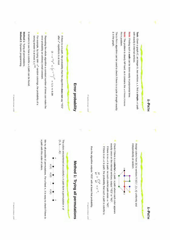
k-P

AT

H

Task:G

ivena

graphG

,aninteger

k,tw

overtices

s,t,find

asim

ple

s-tpath

with

exactlyk

internalvertices.

No

te:F

indingsuch

aw

alkcan

bedone

easilyin

polynomialtim

e.

No

te:T

heproblem

isclearly

NP

-hard,asitcontains

thes-t

HA

MILT

ON

IAN

PA

TH

problem.

The

k-P

AT

Halgorithm

canbe

usedto

checkifthere

isa

cycleoflength

exactlyk

inthe

graph.

FP

Talgorithm

ictechniques

–p.51/97

k-P

AT

H

Assign

colorsfrom

[k]

tovertices

V(G

)\s,t

uniformly

and

independentlyatrandom

.

ts

Check

ifthereis

aco

lorfu

ls-t

path:a

pathw

hereeach

colorappears

exactlyonce

onthe

internalvertices;output“YE

S”

or“N

O”.

Ifthereis

nos-t

k-path:

nosuch

colorfulpathexists⇒

“NO

”.

Ifthereis

ans-t

k-path:

theprobability

thatsucha

pathis

colorfulis

k!

kk

>(

ke)

k

kk

=e−

k,

thusthe

algorithmoutputs

“YE

S”

with

atleastthatprobability.F

PT

algorithmic

techniques–

p.52/97

Erro

rp

rob

ability

Ifthereis

ak

-path,theprobability

thatthealgorithm

do

esn

ot

say“Y

ES

”

aftere

krepetitions

isatm

ost

(1−e−

k)

ek

< (e−

e −k )

ek

=1/e≈

0.3

8

Repeating

thew

holealgorithm

aconstantnum

beroftim

escan

make

the

errorprobability

anarbitrary

smallconstant.

For

example,by

trying100·

ek

randomcolorings,the

probabilityofa

wrong

answer

isatm

ost1/e100.

Itremains

tosee

howa

colorfuls-t

pathcan

befound.

Meth

od

1:Trying

allpermutations.

Meth

od

2:D

ynamic

programm

ing.

FP

Talgorithm

ictechniques

–p.53/97

Meth

od

1:Tryin

gallp

ermu

tation

s

The

colorsencountered

ona

colorfuls-t

pathform

aperm

utationπ

of

1,2,...,k

:

st

π(k

)...

π(2

)π(1

)

We

tryallpossible

k!

permutations.

For

afixed

π,itis

easyto

checkifthere

is

apath

with

thisorder

ofcolors.

FP

Talgorithm

ictechniques

–p.54/97

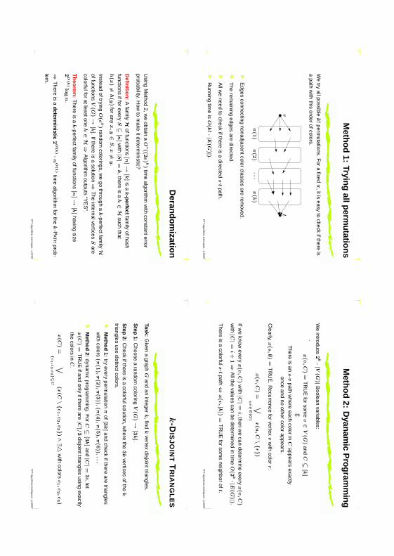
Meth

od

1:Tryin

gallp

ermu

tation

s

We

tryallpossible

k!

permutations.

For

afixed

π,itis

easyto

checkifthere

is

apath

with

thisorder

ofcolors.

st

π(1

)π(2

)...

π(k

)

Edges

connectingnonadjacentcolor

classesare

removed.

The

remaining

edgesare

directed.

Allw

eneed

tocheck

ifthereis

adirected

s-tpath.

Running

time

isO

(k!·|E

(G)|).

FP

Talgorithm

ictechniques

–p.55/97

Meth

od

2:D

yanam

icP

rog

ramm

ing

We

introduce2

k·|V(G

)|B

ooleanvariables:

x(v

,C

)=

TR

UE

forsom

ev∈

V(G

)and

C⊆

[k]

mT

hereis

ans-v

pathw

hereeach

colorin

Cappears

exactly

onceand

noother

colorappears.

Clearly,

x(s

,∅)=

TR

UE

.R

ecurrencefor

vertexv

with

colorr

:

x(v

,C

)=

∨uv∈

E(G

)

x(u

,C\

r)

Ifwe

knowevery

x(v

,C

)w

ith|C|=

i,thenw

ecan

determine

everyx(v

,C

)

with|C

|=

i+

1⇒A

llthevalues

canbe

determined

intim

eO

(2k·|E

(G)|).

There

isa

colorfuls-t

path⇔x(v

,[k

])=

TR

UE

forsom

eneighbor

oft.

FP

Talgorithm

ictechniques

–p.56/97

Deran

do

mizatio

n

Using

Method

2,we

obtaina

O∗((2

e)

k)

time

algorithmw

ithconstanterror

probability.H

owto

make

itdeterministic?

Defi

nitio

n:

Afam

ilyHoffunctions

[n]→

[k]

isa

k-p

erfectfam

ilyofhash

functionsiffor

everyS⊆

[n]

with|S|

=k

,thereis

ah∈H

suchthat

h(x

)6=h(y

)for

anyx

,y∈

S,x6=

y.

Insteadoftrying

O(e

k)

randomcolorings,w

ego

througha

k-perfectfam

ilyHoffunctions

V(G

)→[k

].Ifthere

isa

solution⇒T

heinternalvertices

Sare

colorfulforatleastone

h∈H⇒

Algorithm

outputs“Y

ES

”.

Th

eorem

:T

hereis

ak

-perfectfamily

offunctions[n

]→[k

]having

size2

O(k)lo

gn

.

⇒T

hereis

ad

etermin

istic2

O(k)·

nO

(1)

time

algorithmfor

thek

-PA

TH

prob-

lem.

FP

Talgorithm

ictechniques

–p.57/97

k-D

ISJ

OIN

TT

RIA

NG

LE

S

Task:G

ivena

graphG

andan

integerk

,findk

vertexdisjointtriangles.

Step

1:C

hoosea

randomcoloring

V(G

)→[3

k].

Step

2:C

heckifthere

isa

colorfulsolution,where

the3k

verticesofthe

k

trianglesuse

distinctcolors.

Meth

od

1:try

everyperm

utationπ

of[3

k]

andcheck

ifthereare

triangles

with

colors(π

(1),

π(2

),π(3

)),(π

(4),

π(5

),π(6

)),...

Meth

od

2:dynam

icprogram

ming.

For

C⊆

[3k]

and|C|=

3i,let

x(C

)=

TR

UE

ifandonly

ifthereare|C

|/3

disjointtrianglesusing

exactly

thecolors

inC

.

x(C

)=

∨

c1

,c2

,c3 ⊆

C

(x(C\

c1,c2,c3

)∧∃

with

colorsc1,c2,c3)

FP

Talgorithm

ictechniques

–p.58/97

k-D

ISJ

OIN

TT

RIA

NG

LE

S

Step

3:C

olorfulsolutionexists

with

probabilityatleast

e−

3k,w

hichis

alow

er

boundon

theprobability

ofacorrectansw

er.

Ru

nn

ing

time:

constanterrorprobability

aftere3

krepetitions⇒

runningtim

eis

O∗((2

e)3

k)

(usingM

ethod2).

Deran

do

mizatio

n:3k

-perfectfamily

offunctionsinstead

ofrandomcoloring.

Running

time

is2

O(k)·

nO

(1).

FP

Talgorithm

ictechniques

–p.59/97

Co

lor

cod

ing

We

haveseen

thatcolorcoding

canbe

usedto

findpaths,cycles

oflengthk

,

ora

setofk

disjointtriangles.

Whatother

structurescan

befound

efficientlyw

iththis

technique?

The

keyis

treewidth:

Th

eorem

:G

iventw

ograph

H,G

,itcanbe

decidedif

His

asubgraph

ofG

in

time

2O

(|V(H

)|)·|V(G

)| O(w

),where

wis

thetreew

idthof

G.

Thus

ifH

belongsto

aclass

ofgraphsw

ithbounded

treewidth,then

the

subgraphproblem

isF

PT.

FP

Talgorithm

ictechniques

–p.60/97

Matro

idT

heo

ry

FP

Talgorithm

ictechniques

–p.61/97

Matro

idT

heo

ry

Matroids:

aclassicalsubjectofcom

binatorialoptimization.

Matroids

lurkbehind

matching,flow

,spanningtree,and

some

linear

algebraproblem

s.

AgeneralF

PT

resultthatcanbe

usedto

showthatsom

econcrete

problems

areF

PT.

FP

Talgorithm

ictechniques

–p.62/97

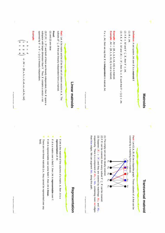
Matro

ids

Defi

nitio

n:

Asetsystem

Mover

Eis

am

atroid

if

(1)∅∈M

.

(2)If

X∈

Mand

Y⊆

X,then

Y∈M

.

(3)If

X,Y∈

Mand|X

|>|Y|,then∃

e∈

Xsuch

thatY∪e∈M

.

Exam

ple:M

=∅

,1,2,3,12,13

isa

matroid.

Exam

ple:M

=∅

,1,2,12,3

isnota

matroid.

Ifx∈M

,thenw

esay

thatX

isin

dep

end

ent

inm

atroidM.

FP

Talgorithm

ictechniques

–p.63/97

Transversalm

atroid

Fact:Let

G(A

,B

;E

)be

abipartite

graph.T

hosesubsets

ofA

thatcanbe

coveredby

am

atchingform

am

atroid.b3

a1

b4

b5

a2

a3

a4

a5

b1

b2

(1)T

heem

ptysetcan

beclearly

covered.

(2)If

Xcan

becovered,then

everysubset

Y⊆

Xcan

becovered.

(3)S

uppose|X|

>|Y|

andthey

arecovered

bym

atchingsM

Xand

MY

,

respectively.T

hereis

acom

ponentof

MX∪

MY

containingm

orered

edges

thanblue

edges.W

ecan

augment

MY

alongthis

path.

FP

Talgorithm

ictechniques

–p.64/97

Lin

earm

atroid

s

Fact:Let

Abe

matrix

andlet

Ebe

thesetofcolum

nvectors

inA

.T

he

subsetsE′⊆

Ethatare

linearlyindependentform

am

atroid.

Pro

of:

(1)and

(2)are

clear.

(3)If|X

|>|Y|

andboth

ofthemare

linearlyindependent,then

Xspans

asubspace

with

largerdim

ensionthan

Y.

Thus

Xcontains

avector

vnot

spannedby

Y⇒

Y∪v

islinearly

independent.

Exam

ple:

ab

cd

1

02

3

01

46

⇒M

=∅

,a,b,c,d,ab,ac,ad,bc,bd

FP

Talgorithm

ictechniques

–p.65/97

Rep

resentatio

n

IfMis

them

atroidofthe

columns

ofam

atrixA

,thenA

isa

represen

tation

ofM

.

IfA

isa

matrix

overa

fieldF

,thenMis

represen

table

overF.

IfMis

representableover

some

fieldF

,thenMis

linear.

There

arenon-linear

matroids

(i.e.,theycannotbe

representedover

any

field).

FP

Talgorithm

ictechniques

–p.66/97

Transversalm

atroid

sare

linear

Fact:Let

G(A

,B

;E

)be

abipartite

graph.T

hosesubsets

ofA

thatcanbe

coveredby

am

atchingform

alinear

matroid.

a1

b5

b4

b3

b2

b1

a5

a4

a3

a2

a1

a2

a3

a4

a5

b1

b2

b3

b4

b5

?0

00

0

??

00

0

0?

0?

0

?0

??

?

00

0?

?

C

onstructthebipartite

adjacencym

atrix:if

ai

andb

jare

neighbors,thenthe

i-thelem

entofrowj

isa

randominteger

between

1and

N.

Elem

entscan

bem

atched⇒T

hedeterm

inantis

nonzerow

ithhigh

probability

(Schw

artz-Zippel)

FP

Talgorithm

ictechniques

–p.67/97

FP

Tresu

lt

Main

result:

LetMbe

alinear

matroid

overE

,givenby

arepresentation

A.

LetSbe

acollection

ofsubsetsof

E,each

ofsizeatm

ostℓ.

Itcanbe

decidedin

randomized

time

f(k

,ℓ)·

nO

(1)

whetherM

hasan

independentsetthatis

theunion

ofk

disjointsetsfrom

S.

Imm

ediate

app

lication

:k

-DIS

JOIN

TT

RIA

NG

LE

Sis

(randomized)

FP

T(letS

bethe

setofalltrianglesin

thegraph).

Two

notsoobvious

applications:

RE

LIA

BL

ET

ER

MIN

AL

S

AS

SIG

NM

EN

TW

ITH

CO

UP

LE

S

FP

Talgorithm

ictechniques

–p.68/97

RE

LIA

BL

ET

ER

MIN

AL

S

LetD

bea

directedgraph

with

asource

vertexs

anda

subsetT

ofvertices.

Task:S

electk

terminals

t1,...,tk∈

T,and

ℓpaths

froms

toeach

ti

suchthatthese

k·ℓ

pathsare

pairwise

internallyvertex

disjoint.

sT

k=

2,ℓ

=3

Th

eorem

:T

heproblem

canbe

solvedin

randomized

time

f(k

,ℓ)·

nO

(1).

FP

Talgorithm

ictechniques

–p.69/97

RE

LIA

BL

ET

ER

MIN

AL

S

Atechnicaltrick:

replaceeach

t∈T

with

ℓcopies,and

replaces

with

aset

S

ofk·ℓ

copies.

ST

k=

2,ℓ

=3

Now

ifaterm

inalt

isselected,then

we

shouldconnectthe

ℓcopies

oft

with

ℓ

differentverticesof

S.

Fact:[P

erfect]LetD

bea

directedgraph

andS

asubsetofvertices.

Those

subsetsX

thatcanbe

reachedfrom

Sby

disjointpathsform

am

atroid.

FP

Talgorithm

ictechniques

–p.70/97

RE

LIA

BL

ET

ER

MIN

AL

S

Fact:[P

erfect]LetD

bea

directedgraph

andS

asubsetofvertices.

Those

subsetsX

thatcanbe

reachedfrom

Sby

disjointpathsform

am

atroid.

The

problemis

equivalenttofinding

kblocks

whose

unionis

independentin

thism

atroid⇒W

ecan

solveitin

randomized

time

f(k

,ℓ)·

nO

(1).

The

matroid

isactually

atransversalm

atroidof

anappropriately

definedbipar-

titegraph,hence

itislinear

andw

ecan

constructarepresentation

forit.

FP

Talgorithm

ictechniques

–p.71/97

AS

SIG

NM

EN

TW

ITH

CO

UP

LE

S

Task:A

ssignpeople

tojobs

(bipartitem

atching).

How

ever,thesetofpeople

includescouples

andthe

mem

bersofa

couplecannotbe

assignedindependently

(say,theyw

anttobe

inthe

same

town).

Task:G

iven

asetofsingles

anda

listofsuitablejobs

foreach

single,

asetofcouples

anda

listofsuitablepairs

ofjobsfor

eachcouple,

assigna

jobto

eachsingle

anda

pairofjobs

toeach

couple.

Th

eorem

:A

SS

IGN

ME

NT

WIT

HC

OU

PL

ES

israndom

izedF

PT

parameterized

bythe

number

kofcouples.

FP

Talgorithm

ictechniques

–p.72/97

AS

SIG

NM

EN

TW

ITH

CO

UP

LE

S

J:

jobs,S

:singles,

C:

couples

LetX⊆

Jbe

inMifand

onlyif

Shas

am

atchingw

ithJ\

X.

Lem

ma:M

ism

atroid.

LetM′

bethe

matroid

overJ∪

Csuch

thatX∈M

′⇔X∩

J∈M

.

C

J

For

eachcouple

c∈C

andsuitable

pairj1,j2

,addtriple

c,j1,j2

toS.

The

kcouples

andallthe

singlescan

bea

assigneda

job

mT

hereare

kdisjointtriples

inSw

hoseunion

isindependentinM

′

FP

Talgorithm

ictechniques

–p.73/97

Cu

tp

rob

lems

FP

Talgorithm

ictechniques

–p.74/97

MU

LTIW

AY

CU

T

Task:G

ivena

graphG

,aset

Tofvertices,and

aninteger

k,find

aset

Sofat

most

kedges

thatseparatesT

(eachcom

ponentofG\

Scontains

atmost

onevertex

ofT

).

Polynom

ialfor|T|=

2,butN

P-hard

for|T|=

3.

Th

eorem

:M

ULT

IWA

YC

UT

isF

PT

parameterized

byk

.

S

YX

δ(R

):setofedges

leavingR

λ(X

,Y

):m

inimum

number

ofedgesin

an(X

,Y

)-separator

FP

Talgorithm

ictechniques

–p.75/97

Su

bm

od

ularity

Fact:T

hefunction

δis

sub

mo

du

lar:for

arbitrarysets

A,B

,

|δ(A

)|+|δ

(B)|≥

|δ(A∩

B)|

+|δ

(A∪

B)|

Pro

of:

Determ

ineseparately

thecontribution

ofthedifferenttypes

ofedges.

BA

FP

Talgorithm

ictechniques

–p.76/97

Su

bm

od

ularity

Co

nseq

uen

ce:T

hereis

aunique

maxim

alR

max ⊇

Xsuch

thatδ(R

max )

isan

(X,Y

)-separatorofsize

λ(X

,Y

).

Pro

of:

LetR

1,R

2 ⊇X

betw

osets

suchthat

δ(R

1),

δ(R

2)

are(X

,Y

)-separatorsofsize

λ:=

λ(X

,Y

).

R2

R1

YX

|δ(R

1)|

+|δ

(R2)|

≥|δ

(R1 ∩

R2)|

+|δ

(R1 ∪

R2)|

λλ

≥λ

⇒|δ

(R1 ∪

R2)|≤

λ

No

te:A

nalogousresultholds

fora

uniquem

inimal

Rm

in .F

PT

algorithmic

techniques–

p.77/97

MU

LTIW

AY

CU

T

Intu

ition

:C

onsidera

t∈T

.A

subsetofthesolution

separatest

andT\

t.

t

There

arem

anysuch

separators.

Buta

separatorfarther

fromt

andcloser

toT\

tseem

sto

bem

oreuseful.

FP

Talgorithm

ictechniques

–p.78/97

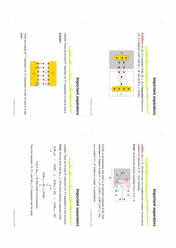
Imp

ortan

tsep

arators

Defi

nitio

n:

An

(X,Y

)-separatorδ(R

)(R⊇

X)

isim

po

rtant

ifthereis

no

(X,Y

)-separatorδ(R

′)w

ithR⊂

R′

and|δ(R

′)|≤|δ

(R)|.

XY

FP

Talgorithm

ictechniques

–p.79/97

Imp

ortan

tsep

arators

Lem

ma:

Lett∈

T.

The

MU

LTIW

AY

CU

Tproblem

hasa

solutionS

suchthat

S

containsan

important

(t,T\

t)-separator.

Pro

of:

LetR

bethe

verticesreachable

fromt

inG\

S.

t

Rv

u

R′

Ifδ(R

)is

notimportant,then

thereis

anim

portantseparatorδ(R

′)that

dominates

it.R

eplaceS

with

S′:=

(S\

δ(R

))∪δ(R

′)(|S

′|≤|S|).

Au

-vpath

inG\

S′

implies

au

-tpath,a

contradiction.F

PT

algorithmic

techniques–

p.80/97

Imp

ortan

tsep

arators

Lem

ma:

There

areatm

ost4

kim

portant(X

,Y

)-separatorsofsize

atmost

k.

Exam

ple:

X Y

k/2

12

There

areexactly

2k

/2

important

(X,Y

)-separatorsof

sizeat

most

kin

this

graph.

FP

Talgorithm

ictechniques

–p.81/97

Imp

ortan

tsep

arators

Lem

ma:

There

areatm

ost4

kim

portant(X

,Y

)-separatorsofsize

atmost

k.

Pro

of:

Firstw

eshow

thatR

max ⊆

Rfor

everyim

portantseparatorδ(R

).

|δ(R

max )|

+|δ

(R)|

≥|δ

(Rm

ax ∩R

)|+

|δ(R

max ∪

R)|

λ≥

λ

⇓|δ

(Rm

ax ∪R

)|≤|δ

(R)|

⇓If

R6=

Rm

ax ∪R

,thenδ(R

)is

notimportant.

Thus

theim

portant(X

,Y

)-and

(Rm

ax ,Y

)-separatorsare

thesam

e.

FP

Talgorithm

ictechniques

–p.82/97

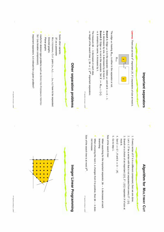
Imp

ortan

tsep

arators

Lem

ma:

There

areatm

ost4

kim

portant(X

,Y

)-separatorsofsize

atmost

k.

XY

Rm

ax

vu

The

edgeu

vleaving

Rm

axis

eitherin

theseparator

ornot.

Bran

ch1:

Edge

uv

isin

theseparator.

Delete

uv

andset

k:=

k−

1.

⇒k

decreasesby

one,λ

decreasesby

atmost

1.

Bran

ch2:

Edge

uv

isnotin

theseparator.

Set

X:=

Rm

ax ∪v

.⇒

krem

ainsthe

same,

λincreases

by1

.

The

measure

2k−

λdecreases

ineach

step.

⇒H

eightofthesearch

tree≤2k⇒≤

22

kim

portantseparators.

FP

Talgorithm

ictechniques

–p.83/97

Alg

orith

mfo

rM

ULT

IWA

YC

UT

1.Ifevery

vertexof

Tis

ina

differentcomponent,then

we

aredone.

2.Let

t∈T

bea

vertexw

iththatis

notseparatedfrom

everyT\

t.

3.B

ranchon

achoice

ofanim

portant(

t,T\

t)

separatorS

ofsizeat

most

k.

4.S

etG

:=G\

Sand

k:=

k−|S|.

5.G

oto

step1.

Size

ofthesearch

tree:

When

searchingfor

theim

portantseparator,2k−

λdecreases

ateachbranching.

When

choosingthe

nextt,

λchanges

from0

topositive,thus

2k−

λdoes

notincrease.

Size

ofthesearch

treeis

atmost

22

k.F

PT

algorithmic

techniques–

p.84/97

Oth

ersep

aration

pro

blem

s

Som

eother

variants:

|T|as

aparam

eter

MU

LTIT

ER

MIN

AL

CU

T:pairs

(s1,t1),

...,

(sℓ ,

tℓ )

haveto

beseparated.

Directed

graphs

Planar

graphs

Usefulfor

deletion-typeproblem

ssuch

asD

IRE

CT

ED

FE

ED

BA

CK

VE

RT

EX

SE

T(via

iterativecom

pression).

Importantseparators:

isitrelevantfor

agiven

problem?

FP

Talgorithm

ictechniques

–p.85/97

Integ

erL

inear

Pro

gram

min

g

FP

Talgorithm

ictechniques

–p.86/97

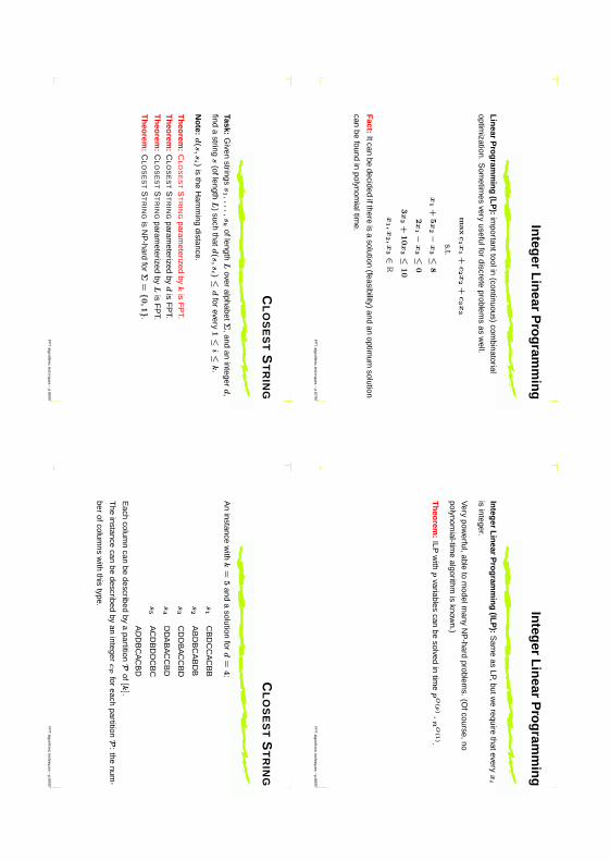
Integ

erL

inear

Pro

gram

min

g

Lin

earP

rog

ramm

ing

(LP

):im

portanttoolin(continuous)

combinatorial

optimization.

Som

etimes

veryusefulfor

discreteproblem

sas

well.

max

c1x

1+

c2x

2+

c3x

3

s.t.

x1+

5x

2 −x

3 ≤8

2x

1 −x

3 ≤0

3x

2+

10x

3 ≤10

x1,x

2,x

3 ∈R

Fact:Itcan

bedecided

ifthereis

asolution

(feasibility)and

anoptim

umsolution

canbe

foundin

polynomialtim

e.

FP

Talgorithm

ictechniques

–p.87/97

Integ

erL

inear

Pro

gram

min

g

Integ

erL

inear

Pro

gram

min

g(IL

P):

Sam

eas

LP,butwe

requirethatevery

xi

isinteger.

Very

powerful,able

tom

odelmany

NP

-hardproblem

s.(O

fcourse,no

polynomial-tim

ealgorithm

isknow

n.)

Th

eorem

:ILP

with

pvariables

canbe

solvedin

time

pO

(p)·

nO

(1).

FP

Talgorithm

ictechniques

–p.88/97

CL

OS

ES

TS

TR

ING

Task:G

ivenstrings

s1 ,

...,

sk

oflengthL

overalphabet

Σ,and

aninteger

d,

finda

strings

(oflengthL

)such

thatd(s

,s

i )≤d

forevery

1≤

i≤k

.

No

te:d(s

,s

i )is

theH

amm

ingdistance.

Th

eorem

:C

LO

SE

ST

ST

RIN

Gparam

eterizedby

kis

FP

T.

Th

eorem

:C

LO

SE

ST

ST

RIN

Gparam

eterizedby

dis

FP

T.T

heo

rem:

CL

OS

ES

TS

TR

ING

parameterized

byL

isF

PT.

Th

eorem

:C

LO

SE

ST

ST

RIN

Gis

NP

-hardfor

Σ=0,1

.

FP

Talgorithm

ictechniques

–p.89/97

CL

OS

ES

TS

TR

ING

An

instancew

ithk

=5

anda

solutionfor

d=

4:

s1

CB

DC

CA

CB

B

s2

AB

DB

CA

BD

B

s3

CD

DB

AC

CB

D

s4

DD

AB

AC

CB

D

s5

AC

DB

DD

CB

C

AD

DB

CA

CB

D

Each

column

canbe

describedby

apartitionP

of[k

].

The

instancecan

bedescribed

byan

integercP

foreach

partitionP:

thenum

-

berofcolum

nsw

iththis

type.

FP

Talgorithm

ictechniques

–p.90/97

CL

OS

ES

TS

TR

ING

Each

column

canbe

describedby

apartitionP

of[k

].

The

instancecan

bedescribed

byan

integercP

foreach

partitionP:

thenum

berofcolum

nsw

iththis

type.

Describ

ing

aso

lutio

n:

IfC

isa

classofP

,letxP

,Cbe

thenum

beroftypeP

columns

where

thesolution

agreesw

ithclass

C.

There

isa

solutioniffthe

following

ILPhas

afeasible

solution:∑C∈P

xP

,C≤

cP∀

partitionP∑i6∈

C,C∈P

xP

,C≤

d∀1≤

i≤k

xP

,C≥

0∀P

,C

Num

berofvariables

is≤B

(k)·

k,w

hereB

(k)

isthe

no.ofpartitionsof

[k]

⇒T

heILP

algorithmsolves

theproblem

intim

ef(k

)·n

O(1).

FP

Talgorithm

ictechniques

–p.91/97

ST

EIN

ER

TR

EE

FP

Talgorithm

ictechniques

–p.92/97

ST

EIN

ER

TR

EE

Task:G

ivena

graphG

with

weighted

edgesand

aset

Sof

kvertices,find

a

treeT

ofminim

umw

eightthatcontainsS

.

Know

nto

beN

P-hard.

For

fixedk

,we

cansolve

itinpolynom

ialtime:

we

can

guessthe

Steiner

pointsand

thew

aythey

areconnected.

Th

eorem

:S

TE

INE

RT

RE

Eis

FP

Tparam

eterizedby

k=|S|.

FP

Talgorithm

ictechniques

–p.93/97

ST

EIN

ER

TR

EE

Solution

bydynam

icprogram

ming.

For

v∈

V(G

)and

X⊆

S,

c(v

,X

):=

minim

umcostofa

Steiner

treeof

Xthatcontains

v

d(u

,v):=

distanceof

uand

v

Recu

rrence

relation

:

c(v

,X

)=

min

u∈

V(G

)

∅⊂X′⊂

X

c(u

,X′\

u)+

c(u

,(X\

X′)\

u)+

d(u

,v)

FP

Talgorithm

ictechniques

–p.94/97

ST

EIN

ER

TR

EE

Recu

rrence

relation

:

c(v

,X

)=

min

u∈

V(G

)

∅⊂X′⊂

X

c(u

,X′\

u)+

c(u

,(X\

X′)\

u)+

d(u

,v)

≤:

Atree

T1

realizingc(u

,X′\

u),

atree

T2

realizingc(u

,(X\

X′)\

u),and

thepath

uv

givesa

(supersetofa)Steiner

treeof

Xcontaining

v.

v

T2

T1

uFP

Talgorithm

ictechniques

–p.95/97

ST

EIN

ER

TR

EE

Recu

rrence

relation

:

c(v

,X

)=

min

u∈

V(G

)

∅⊂X′⊂

X

c(u

,X′\

u)+

c(u

,(X\

X′)\

u)+

d(u

,v)

≥:

Suppose

Trealizes

c(v

,X

),letT′

be

them

inimum

subtreecontaining

X.

Letu

bea

vertexof

T′

closesttov

.If|X

|>

1,

thenthere

isa

component

Cof

T\

uthat

containsa

subset∅⊂

X′⊂

Xof

termi-

nals.T

husT

isthe

disjointunionofa

treecontaining

X′\

uand

u,a

treecontaining

(X\

X′)\

uand

u,and

thepath

uv

.v

T1

T2

uFP

Talgorithm

ictechniques

–p.95/97

ST

EIN

ER

TR

EE

Recu

rrence

relation

:

c(v

,X

)=

min

u∈

V(G

)

∅⊂X′⊂

X

c(u

,X′\

u)+

c(u

,(X\

u)\

X′)

+d(u

,v)

Ru

nn

ing

time:

2k|V

(G)|

variablesc(v

,X

),determine

themin

increasingorder

of|X|.

Variable

c(v

,X

)can

bedeterm

inedby

considering2|X|

cases.Totalnum

ber

ofcasesto

consider:

∑X⊆

T

2|X|=

k∑i=

1 (ki )

2i≤

(1+

2)

k=

3k.

Running

time

isO∗(3

k).

No

te:R

unningtim

ecan

bereduced

toO∗(2

k)

with

clevertechniques.

FP

Talgorithm

ictechniques

–p.96/97

Co

nclu

sion

s

Many

nicetechniques

inventedso

far—

andprobably

many

more

tocom

e.

Asingle

techniquem

ightprovidethe

keyfor

severalproblems.

How

tofind

newtechniques?

By

attackingthe

openproblem

s!

Needed:

flexible,highlyexpressive

problems.

Solve

otherproblem

sby

reductionto

theseproblem

s.

Courcelle’s

Theorem

The

matroid

result

2S

AT

DE

LE

TIO

N:

givena

2SAT

formula

andan

integerk

,deletek

clausesto

make

itsatisfiable

ConstraintS

atisfactionP

roblems

FP

Talgorithm

ictechniques

–p.97/97

Saket Saurabh

Kernel : Lower and UpperBounds

Kernel: Lower and Upper Bounds

Daniel Lokshtanov∗ Saket Saurabh∗

May 21, 2009

Abstract

Through this lecture note we try to provide a portal into the emerging filed of ker-nelization. We exhibit through examples various tools to prove both lower and upperbounds on the kernel sizes.

1 Introduction

Preprocessing (data reduction or kernelization) as a strategy of coping with hard problems isuniversally used in almost every implementation. The history of preprocessing, like applyingreduction rules to simplify truth functions, can be traced back to the 1950’s [16]. A naturalquestion in this regard is how to measure the quality of preprocessing rules proposed for aspecific problem. For a long time the mathematical analysis of polynomial time preprocess-ing algorithms was neglected. The basic reason for this anomaly was that if we start withan instance I of an NP-hard problem and can show that in polynomial time we can replacethis with an equivalent instance I ′ with |I ′| < |I| then that would imply P=NP in classi-cal complexity. The situation changed drastically with advent of parameterized complexity.Combining tools from parameterized complexity and classical complexity it has become pos-sible to derive upper and lower bounds on the sizes of reduced instances, or so called kernels.Importance of preprocessing and the mathematical challenges it poses is beautifully expressedin the following quote by Fellows.

It has become clear, however, that far from being trivial and uninteresting, thatpre-processing has unexpected practical power for real world input distributions,and is mathematically a much deeper subject than has generally been understood.

Working View Point on Kernel: In parameterized complexity each problem instancecomes with a parameter k and the parameterized problem is said to admit a polynomialkernel if there is a polynomial time algorithm (the degree of polynomial is independent ofk), called a kernelization algorithm, that reduces the input instance down to an instancewith size bounded by a polynomial p(k) in k, while preserving the answer. This reducedinstance is called a p(k) kernel for the problem. If p(k) = O(k), then we call it a linearkernel. Kernelization has been extensively studied in the realm of parameterized complexity,

∗Department of Infomatics, University of Bergen, Norway. daniello|saket.saurabh@ii.uib.no.

1

resulting in polynomial kernels for a variety of problems. Notable examples include a 2k-sized vertex kernel for Vertex Cover [6], a 355k kernel for Dominating Set on planargraphs [1], which later was improved to a 67k kernel [5], and an O(k2) kernel for Feedback

Vertex Set [18] parameterized by the solution size.

2 Basic Definitions

A parameterized problem L is a subset of Σ∗×N for some finite alphabet Σ. An instance ofa parameterized problem consists of (x, k), where k is called the parameter. A central notionin parameterized complexity is fixed parameter tractability (FPT) which means for a giveninstance (x, k) solvability in time f(k) · p(|x|), where f is an arbitrary function of k and p

is a polynomial in the input size. The notions of kernelization and composition are formallydefined as follows.

Definition 1. A kernelization algorithm, or in short, a kernel for a parameterized problemQ ⊆ Σ∗ × N is an algorithm that, given (x, k) ∈ Σ∗ × N, outputs in time polynomial in|x| + k a pair (x′, k′) ∈ Σ∗ × N such that (a) (x, k) ∈ Q if and only if (x′, k′) ∈ Q and (b)|x′|+k′ ≤ g(k), where g is an arbitrary computable function. The function g is referred to asthe size of the kernel. If g is a polynomial function then we say that Q admits a polynomialkernel.

We close with some definitions from graph theory. Let G = (V,E) be a graph. For avertex v in G, we write NG(v) to denote the set of v’s neighbors in G, and we write degG(v)to denote the degree of v, that is, the number of v’s neighbors in G. If it is clear fromthe context which graph is meant, we write N(v) and deg(v), respectively, for short. Agraph G′ = (V ′, E′) is a subgraph of G if V ′ ⊆ V and E′ ⊆ E. The subgraph G′ is calledan induced subgraph of G if E′ = u, v ∈ E | u, v ∈ V ′, in this case, G′ is also called thesubgraph induced by V ′ and denoted with G[V ′]. A vertex v dominates a vertex u if u ∈ N(v).

3 Upper Bound Machinery

We illustrate the method of kernelization using the parameterized version of Max3Sat wheregiven a boolean 3-CNF formula and an integer parameter k, we would like to know whetherthere is an assignment to the variables that satisfies at least k of the clauses. Our otherexamples in this Section include a kernel for d-Hitting Set using the Sunflower Lemma, a4k sized kernel for Vertex Cover using crown decomposition and a 2k kernel for (Edge)

Clique Cover.

3.1 Max3Sat

Let F be a given boolean CNF 3-SAT formula with n variables and m clauses. t is well knownthat in any boolean CNF formula, there is an assignment that satisfies at least half of theclauses (given any assignment that doesn’t satisfy half the clauses, its bitwise complementwill). So if the parameter k is less than m/2, then there is an assignment to the variablesthat satisfies at least k of the clauses. Otherwise, m ≤ 2k, and so n ≤ 6k.

2

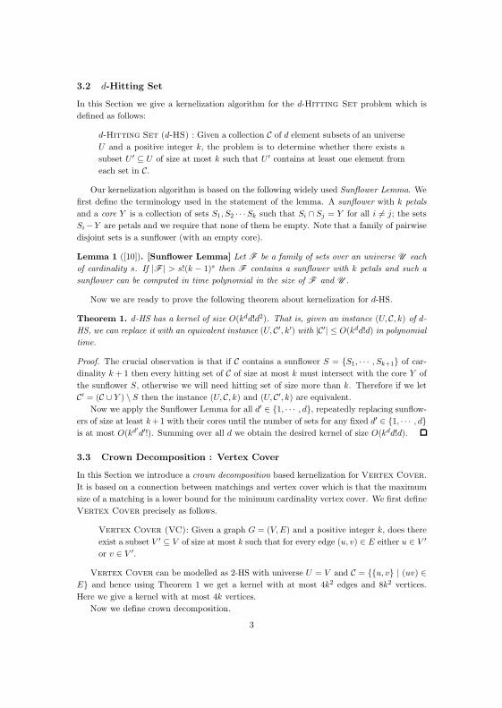
3.2 d-Hitting Set

In this Section we give a kernelization algorithm for the d-Hitting Set problem which isdefined as follows:

d-Hitting Set (d-HS) : Given a collection C of d element subsets of an universeU and a positive integer k, the problem is to determine whether there exists asubset U ′ ⊆ U of size at most k such that U ′ contains at least one element fromeach set in C.

Our kernelization algorithm is based on the following widely used Sunflower Lemma. Wefirst define the terminology used in the statement of the lemma. A sunflower with k petalsand a core Y is a collection of sets S1, S2 · · ·Sk such that Si ∩ Sj = Y for all i 6= j; the setsSi−Y are petals and we require that none of them be empty. Note that a family of pairwisedisjoint sets is a sunflower (with an empty core).

Lemma 1 ([10]). [Sunflower Lemma] Let F be a family of sets over an universe U eachof cardinality s. If |F | > s!(k − 1)s then F contains a sunflower with k petals and such asunflower can be computed in time polynomial in the size of F and U .

Now we are ready to prove the following theorem about kernelization for d-HS.

Theorem 1. d-HS has a kernel of size O(kdd!d2). That is, given an instance (U, C, k) of d-HS, we can replace it with an equivalent instance (U, C′, k′) with |C′| ≤ O(kdd!d) in polynomialtime.

Proof. The crucial observation is that if C contains a sunflower S = S1, · · · , Sk+1 of car-dinality k + 1 then every hitting set of C of size at most k must intersect with the core Y ofthe sunflower S, otherwise we will need hitting set of size more than k. Therefore if we letC′ = (C ∪ Y ) \ S then the instance (U, C, k) and (U, C′, k) are equivalent.

Now we apply the Sunflower Lemma for all d′ ∈ 1, · · · , d, repeatedly replacing sunflow-ers of size at least k +1 with their cores until the number of sets for any fixed d′ ∈ 1, · · · , dis at most O(kd′d′!). Summing over all d we obtain the desired kernel of size O(kdd!d).

3.3 Crown Decomposition : Vertex Cover

In this Section we introduce a crown decomposition based kernelization for Vertex Cover.It is based on a connection between matchings and vertex cover which is that the maximumsize of a matching is a lower bound for the minimum cardinality vertex cover. We first defineVertex Cover precisely as follows.

Vertex Cover (VC): Given a graph G = (V,E) and a positive integer k, does thereexist a subset V ′ ⊆ V of size at most k such that for every edge (u, v) ∈ E either u ∈ V ′

or v ∈ V ′.

Vertex Cover can be modelled as 2-HS with universe U = V and C = u, v | (uv) ∈E and hence using Theorem 1 we get a kernel with at most 4k2 edges and 8k2 vertices.Here we give a kernel with at most 4k vertices.

Now we define crown decomposition.

3

Definition 2. A crown decomposition of a graph G = (V,E) is a partitioning of V as C, H

and R, where C and H are nonempty and the partition satisfies the following properties.

1. C is an independent set.

2. There are no edges between vertices of C and R, that is N [C] ∩R = ∅.3. Let E′ be the set of edges between vertices of C and H. Then E′ contains a matching

of size |H|, that is the bipartite subgraph G′ = (C ∪H,E′) has a matching saturatingall the vertices of H.

We need the following lemma by Chor et. al. [7] which makes it possible to find a crowndecomposition efficiently.

Lemma 2. If a graph G = (V,E) has an independent set I ⊆ V such that |N(I)| < |I|, thena crown decomposition (C,H,R) of G such that C ⊆ I can be found in time O(m+n), givenG and I.

The crown-decomposition gives us a global method to reduce the instance size. Its im-portance is evident from the following simple lemma.

Lemma 3. Let (C,H,R) be a crown decomposition of a graph G = (V,E). Then G has avertex cover of size k if and only if G′ = G[R] has a vertex cover of size k′ = k − |H|.Proof. Suppose G has a vertex cover V ′ of size k in G. Now, we have a matching of size |H|between C and H that saturates every vertex of H. Thus |V ′∩ (H ∪C)| ≥ |H|, as any vertexcover must pick one vertex form each of the matching edge. Hence the number of vertices inV ′ covering the edges not incident to H ∪C is at most k − |H|, proving one direction of theresult.

For the other direction, it is enough to observe that if V ′′ is a vertex cover of size k− |H|for G′ then V ′′ ∪H is a vertex cover of size k for G.

Theorem 2. Vertex Cover has a kernel of size 4k.

Proof. Given an input graph G = (V,E) and a positive integer k, we do as follows. Wefirst find a maximal matching M of G. Let V (M) be the set of endpoints of edges in M .Now if |V (M)| > 2k, we answer NO and stop as any vertex cover must contain at least onevertex from each of the matching edges and hence has size more than k. Now we distinguishtwo cases based on the size of |V − V (M)|. If |V − V (M)| ≤ 2k, then we stop as we haveobtained a kernel of size at most 4k. Else |V − V (M)| > 2k. In this case we have found anindependent set I = V − V (M) such that |N(I)| ≤ |V (M)| < |I| and hence we can applyLemma 2 to obtain a crown decomposition (C,H,R) of G. Given a crown decomposition(C,H,R), we apply Lemma 3 and obtain a smaller instance for a vertex cover with G′ = G[R]and parameter k′ = k− |H|. Now we repeat the above procedure with this reduced instanceuntil either we get a NO answer or we have |V − V (M)| ≤ 2k resulting in a kernel of size4k.

The bound obtained on the kernel for Vertex Cover in Theorem 2 can be furtherimproved to 2k with much more sophisticated use of crown decomposition. An alternatemethod to obtain a 2k size kernel for Vertex Cover is through a Linear Programmingformulation of Vertex Cover. See [10] and [15] for further details on Linear Programmingbased kernelization of Vertex Cover.

4

3.4 Clique Cover

Unfortunately, not all known problem kernels are shown to have polynomial size. Here, wepresent some data reduction results with exponential-size kernels. Clearly, it is a pressingchallenge to find out whether these bounds can be improved to polynomial ones.

In this section, we study the (Edge) Clique Cover problem, where the input consistsof an undirected graph G = (V,E) and a nonnegative integer k and the question is whetherthere is a set of at most k cliques in G such that each edge in E has both its endpoints in atleast one of the selected cliques.

Given an n-vertex and m-edge graph G, we use N(v) to denote the neighborhood ofvertex v in G, namely, N(v) := u | u, v ∈ E. The closed neighborhood of vertex v,denoted by N [v], is equal to N(v) ∪ v.

We formulate data reduction rules for a generalized version of (Edge) Clique Cover

in which already some edges may be marked as “covered”. Then, the question is to find aclique cover of size k that covers all uncovered edges. We apply the following data reductionrules [14]:1. Remove isolated vertices and vertices that are only adjacent to covered edges.2. If an uncovered edge u, v is contained in exactly one maximal clique C, that is, if the

common neighbors of u and v induce a clique, then add C to the solution, mark its edgesas covered, and decrease k by one.

3. If there is an edge u, v whose endpoints have exactly the same closed neighborhood, thatis, N [u] = N [v], then mark all edges incident to u as covered. To reconstruct a solutionfor the non-reduced instance, add u to every clique containing v.The correctness of the rules is easy to prove. To show the following problem kernel, only

the first and third rule are needed.

Theorem 3 ([14]). (Edge) Clique Cover admits a problem kernel with at most 2k ver-tices.

Proof. Consider any graph G = (V,E) with more than 2k vertices that has a clique cover C1, . . . , Ck

of size k. We assign to each vertex v ∈ V a binary vector bv of length k where bit i, 1 ≤ i ≤ k,is set to 1 iff v is contained in clique Ci. Since there are only 2k possible vectors, there mustbe u 6= v ∈ V with bu = bv. If bu and bv are zero, the first rule applies; otherwise, u and v

are contained in the same cliques. This means that u and v are connected and share thesame neighborhood, and thus the third rule applies.

4 Lower Bound Machinery

It is easy to see that if a decidable problem admits an f(k) kernel for some function f , thenthe problem is FPT. Interestingly, the converse also holds, that is, if a problem is FPT thenit admits an f(k) kernel for some function f [15]. The proof of this fact is quite simple, andwe present it here.

Fact 1 (Folklore, [15]). If a parameterized problem Π is FPT then Π admits an f(k) kernelfor some function f .

5

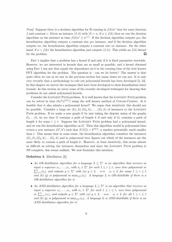
Proof. Suppose there is a decision algorithm for Π running in f(k)nc time for some functionf and constant c. Given an instance (I, k) with |I| = n, if n ≥ f(k) then we run the decisionalgorithm on the instance in time f(k)nc ≤ nc+1. If the decision algorithm outputs yes, thekernelization algorithm outputs a constant size yes instance, and if the decision algorithmoutputs no, the kernelization algorithm outputs a constant size no instance. On the otherhand, if n < f(k) the kernelization algorithm just outputs (I, k). This yields an f(k) kernelfor the problem.

Fact 1 implies that a problem has a kernel if and only if it is fixed parameter tractable.However, we are interested in kernels that are as small as possible, and a kernel obtainedusing Fact 1 has size that equals the dependence on k in the running time of the best knownFPT algorithm for the problem. The question is - can we do better? The answer is thatquite often we can as we saw in the previous section but many times we can not. It is onlyvery recently that a methodology to rule out polynomial kernels has been developed [3, 12].In this chapter we survey the tecniques that have been developed to show kernelization lowerbounds. In this section we suvey some of the recently developed techniques for showing thatproblems do not admit polynomial kernels.

Consider the Longest Path problem. It is well known that the Longest Path problemcan be solved in time O(cknO(1)) using the well known method of Color-Coding. Is itfeasible that it also admits a polynomial kernel? We argue that intuitively this should notbe possible. Consider a large set (G1, k), (G2, k), . . . , (Gt, k) of instances to the Longest

Path problem. If we make a new graph G by just taking the disjoint union of the graphsG1 . . . Gt we see that G contains a path of length k if and only if Gi contains a path oflength k for some i ≤ t. Suppose the Longest Path problem had a polynomial kernel,and we ran the kernelization algorithm on G. Then this algorithm would in polynomial timereturn a new instance (G′, k′) such that |V (G)| = kO(1), a number potentially much smallerthan t. This means that in some sense, the kernelization algorithm considers the instances(G1, k), (G2, k) . . . (Gt, k) and in polynomial time figures out which of the instances are themost likely to contain a path of length k. However, at least intuitively, this seems almostas difficult as solving the instances themselves and since the Longest Path problem isNP-complete, this seems unlikely. We now formalize this intuition.

Definition 3. [Distillation [3]]

• An OR-distillation algorithm for a language L ⊆ Σ∗ is an algorithm that receives asinput a sequence x1, . . . , xt, with xi ∈ Σ∗ for each 1 ≤ i ≤ t, uses time polynomial in∑t

i=1 |xi|, and outputs y ∈ Σ∗ with (a) y ∈ L ⇐⇒ xi ∈ L for some 1 ≤ i ≤ t

and (b) |y| is polynomial in maxi≤t |xi|. A language L is OR-distillable if there is aOR-distillation algorithm for it.

• An AND-distillation algorithm for a language L ⊆ Σ∗ is an algorithm that receives asinput a sequence x1, . . . , xt, with xi ∈ Σ∗ for each 1 ≤ i ≤ t, uses time polynomialin

∑ti=1 |xi|, and outputs y ∈ Σ∗ with (a) y ∈ L ⇐⇒ xi ∈ L for all 1 ≤ i ≤ t

and (b) |y| is polynomial in maxi≤t |xi|. A language L is AND-distillable if there is anAND-distillation algorithm for it.

6

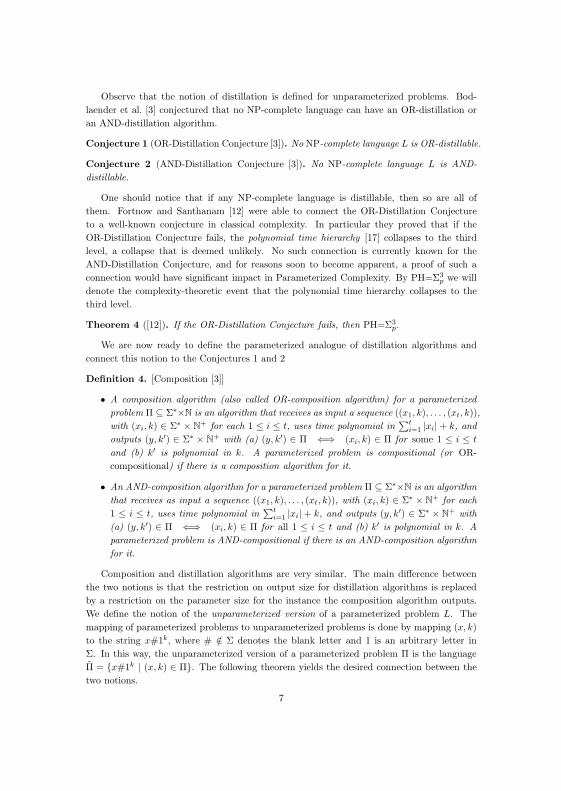
Observe that the notion of distillation is defined for unparameterized problems. Bod-laender et al. [3] conjectured that no NP-complete language can have an OR-distillation oran AND-distillation algorithm.

Conjecture 1 (OR-Distillation Conjecture [3]). No NP-complete language L is OR-distillable.

Conjecture 2 (AND-Distillation Conjecture [3]). No NP-complete language L is AND-distillable.

One should notice that if any NP-complete language is distillable, then so are all ofthem. Fortnow and Santhanam [12] were able to connect the OR-Distillation Conjectureto a well-known conjecture in classical complexity. In particular they proved that if theOR-Distillation Conjecture fails, the polynomial time hierarchy [17] collapses to the thirdlevel, a collapse that is deemed unlikely. No such connection is currently known for theAND-Distillation Conjecture, and for reasons soon to become apparent, a proof of such aconnection would have significant impact in Parameterized Complexity. By PH=Σ3

p we willdenote the complexity-theoretic event that the polynomial time hierarchy collapses to thethird level.

Theorem 4 ([12]). If the OR-Distillation Conjecture fails, then PH=Σ3p.

We are now ready to define the parameterized analogue of distillation algorithms andconnect this notion to the Conjectures 1 and 2

Definition 4. [Composition [3]]

• A composition algorithm (also called OR-composition algorithm) for a parameterizedproblem Π ⊆ Σ∗×N is an algorithm that receives as input a sequence ((x1, k), . . . , (xt, k)),with (xi, k) ∈ Σ∗ × N+ for each 1 ≤ i ≤ t, uses time polynomial in

∑ti=1 |xi| + k, and

outputs (y, k′) ∈ Σ∗ × N+ with (a) (y, k′) ∈ Π ⇐⇒ (xi, k) ∈ Π for some 1 ≤ i ≤ t

and (b) k′ is polynomial in k. A parameterized problem is compositional (or OR-compositional) if there is a composition algorithm for it.

• An AND-composition algorithm for a parameterized problem Π ⊆ Σ∗×N is an algorithmthat receives as input a sequence ((x1, k), . . . , (xt, k)), with (xi, k) ∈ Σ∗ × N+ for each1 ≤ i ≤ t, uses time polynomial in

∑ti=1 |xi| + k, and outputs (y, k′) ∈ Σ∗ × N+ with

(a) (y, k′) ∈ Π ⇐⇒ (xi, k) ∈ Π for all 1 ≤ i ≤ t and (b) k′ is polynomial in k. Aparameterized problem is AND-compositional if there is an AND-composition algorithmfor it.

Composition and distillation algorithms are very similar. The main difference betweenthe two notions is that the restriction on output size for distillation algorithms is replacedby a restriction on the parameter size for the instance the composition algorithm outputs.We define the notion of the unparameterized version of a parameterized problem L. Themapping of parameterized problems to unparameterized problems is done by mapping (x, k)to the string x#1k, where # /∈ Σ denotes the blank letter and 1 is an arbitrary letter inΣ. In this way, the unparameterized version of a parameterized problem Π is the languageΠ = x#1k | (x, k) ∈ Π. The following theorem yields the desired connection between thetwo notions.

7

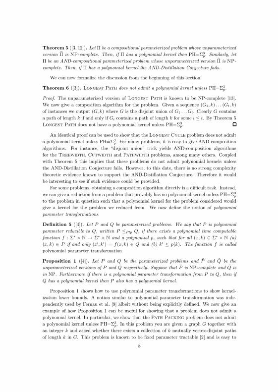
Theorem 5 ([3, 12]). Let Π be a compositional parameterized problem whose unparameterizedversion Π is NP-complete. Then, if Π has a polynomial kernel then PH=Σ3

p. Similarly, letΠ be an AND-compositional parameterized problem whose unparameterized version Π is NP-complete. Then, if Π has a polynomial kernel the AND-Distillation Conjecture fails.

We can now formalize the discussion from the beginning of this section.

Theorem 6 ([3]). Longest Path does not admit a polynomial kernel unless PH=Σ3p.

Proof. The unparameterized version of Longest Path is known to be NP-complete [13].We now give a composition algorithm for the problem. Given a sequence (G1, k) . . . (Gt, k)of instances we output (G, k) where G is the disjoint union of G1 . . . Gt. Clearly G containsa path of length k if and only if Gi contains a path of length k for some i ≤ t. By Theorem 5Longest Path does not have a polynomial kernel unless PH=Σ3

p.

An identical proof can be used to show that the Longest Cycle problem does not admita polynomial kernel unless PH=Σ3

p. For many problems, it is easy to give AND-compositionalgorithms. For instance, the “disjoint union” trick yields AND-composition algorithmsfor the Treewidth, Cutwidth and Pathwidth problems, among many others. Coupledwith Theorem 5 this implies that these problems do not admit polynomial kernels unlessthe AND-Distillation Conjecture fails. However, to this date, there is no strong complexitytheoretic evidence known to support the AND-Distillation Conjecture. Therefore it wouldbe interesting to see if such evidence could be provided.

For some problems, obtaining a composition algorithm directly is a difficult task. Instead,we can give a reduction from a problem that provably has no polynomial kernel unless PH=Σ3

p

to the problem in question such that a polynomial kernel for the problem considered wouldgive a kernel for the problem we reduced from. We now define the notion of polynomialparameter transformations.

Definition 5 ([4]). Let P and Q be parameterized problems. We say that P is polynomialparameter reducible to Q, written P ≤Ptp Q, if there exists a polynomial time computablefunction f : Σ∗ × N → Σ∗ × N and a polynomial p, such that for all (x, k) ∈ Σ∗ × N (a)(x, k) ∈ P if and only (x′, k′) = f(x, k) ∈ Q and (b) k′ ≤ p(k). The function f is calledpolynomial parameter transformation.

Proposition 1 ([4]). Let P and Q be the parameterized problems and P and Q be theunparameterized versions of P and Q respectively. Suppose that P is NP-complete and Q isin NP. Furthermore if there is a polynomial parameter transformation from P to Q, then ifQ has a polynomial kernel then P also has a polynomial kernel.

Proposition 1 shows how to use polynomial parameter transformations to show kernel-ization lower bounds. A notion similar to polynomial parameter transformation was inde-pendently used by Fernau et al. [9] albeit without being explicitly defined. We now give anexample of how Proposition 1 can be useful for showing that a problem does not admit apolynomial kernel. In particular, we show that the Path Packing problem does not admita polynomial kernel unless PH=Σ3

p. In this problem you are given a graph G together withan integer k and asked whether there exists a collection of k mutually vertex-disjoint pathsof length k in G. This problem is known to be fixed parameter tractable [2] and is easy to

8

see that for this problem the “disjoint union” trick discussed earlier does not directly apply.Thus we resort to polynomial parameter transformations.

Theorem 7. Path Packing does not admit a polynomial kernel unless PH=Σ3p.

Proof. We give a polynomial parameter transformation from the Longest Path problem.Given an instance (G, k) to Longest Path we construct a graph G′ from G by adding k−1vertex disjoint paths of length k. Now G contains a path of length k if and only if G′ containsk paths of length k. This concludes the proof.

Now we give several non-trivial applications of this framework developed by Bodlaender etal. [3] and Fortnow and Santhanam [12]. In particular we describe a “cookbook” for showingkernelization lower bounds using explicit identification. We then apply this cookbook to showthat a wide variety of problems do not admit polynomial kernels. To show that a problemdoes not admit a polynomial size kernel we go through the following steps.

1. Find a suitable parameterization of the problem considered. Quite often parameteri-zations that impose extra structure make it easier to give a composition algorithm.

2. Define a suitable colored version of the problem. This is in order to get more controlover how solutions to problem instances can look.

3. Show that the colored version of the problem is NP-complete.

4. Give a polynomial parameter transformation from the colored to the uncolored version.This will imply that if the uncolored version has a polynomial kernel then so doesthe colored version. Hence kernelization lower bounds for the colored version directlytransfer to the original problem.

5. Show that the colored version parameterized by k is solvable in time 2kc · nO(1) for afixed constant c.

6. Finally, show that the colored version is compositional and thus has no polynomialkernel. To do so, proceed as follows.

(a) If the number of instances in the input to the composition algorithm is at least 2kc

then running the parameterized algorithm on each instance takes time polynomialin input size. This automatically yields a composition algorithm.

(b) If the number of instances is less than 2kc, every instance receives an unique

identifier. Notice that in order to uniquely code the identifiers (ID) of all instances,kc bits per instance is sufficient. The IDs are coded either as an integer, or as asubset of a poly(k) sized set.

(c) Use the coding power provided by colors and IDs to complete the compositionalgorithm.

In the following sections we show how to apply this approach to show incompressibility andkernelization lower bounds for a variety of problems.

9

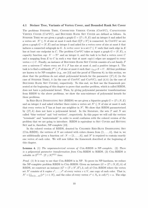
4.1 Steiner Tree, Variants of Vertex Cover, and Bounded Rank Set Cover

The problems Steiner Tree, Connected Vertex Cover (ConVC), Capacitated

Vertex Cover (CapVC), and Bounded Rank Set Cover are defined as follows. InSteiner Tree we are given a graph a graph G = (T ∪N,E) and an integer k and asked fora vertex set N ′ ⊆ N of size at most k such that G[T ∪N ′] is connected. In ConVC we aregiven a graph G = (V,E) and an integer k and asked for a vertex cover of size at most k thatinduces a connected subgraph in G. A vertex cover is a set C ⊆ V such that each edge in E

has at least one endpoint in C. The problem CapVC takes as input a graph G = (V,E), acapacity function cap : V → N+ and an integer k, and the task is to find a vertex cover C

and a mapping from E to C in such a way that at most cap(v) edges are mapped to everyvertex v ∈ C. Finally, an instance of Bounded Rank Set Cover consists of a set family Fover a universe U where every set S ∈ F has size at most d, and a positive integer k. Thetask is to find a subfamily F ′ ⊆ F of size at most k such that ∪S∈F ′S = U . All four problemsare known to be NP-complete (e.g., see [13] and the proof of Theorem 8); in this section, weshow that the problems do not admit polynomial kernels for the parameter (|T |, k) (in thecase of Steiner Tree), k (in the case of ConVC and CapVC), and (d, k) (in the case ofBounded Rank Set Cover), respectively. To this end, we first use the framework pre-sented at the beginning of this chapter to prove that another problem, which is called RBDS,does not have a polynomial kernel. Then, by giving polynomial parameter transformationsfrom RBDS to the above problems, we show the non-existence of polynomial kernels forthese problems.

In Red-Blue Dominating Set (RBDS) we are given a bipartite graph G = (T ∪N,E)and an integer k and asked whether there exists a vertex set N ′ ⊆ N of size at most k suchthat every vertex in T has at least one neighbor in N ′. We show that RBDS parameterizedby (|T |, k) does not have a polynomial kernel. In the literature, the sets T and N arecalled “blue vertices” and “red vertices”, respectively. In this paper we will call the vertices“terminals” and “nonterminals” in order to avoid confusion with the colored version of theproblem that we are going to introduce. RBDS is equivalent to Set Cover and Hitting

Set and is, therefore, NP-complete [13].In the colored version of RBDS, denoted by Colored Red-Blue Dominating Set

(Col-RBDS), the vertices of N are colored with colors chosen from 1, . . . , k, that is, weare additionally given a function col : N → 1, . . . , k, and N ′ is required to contain exactlyone vertex of each color. We will now follow the framework described at the beginning ofthis chapter.

Lemma 4. (1) The unparameterized version of Col-RBDS is NP-complete. (2) Thereis a polynomial parameter transformation from Col-RBDS to RBDS. (3) Col-RBDS issolvable in 2|T |+k · |T ∪N |O(1) time.

Proof. (1) It is easy to see that Col-RBDS is in NP. To prove its NP-hardness, we reducethe NP-complete problem RBDS to Col-RBDS: Given an instance (G = (T ∪N,E), k) ofRBDS, we construct an instance (G′ = (T ∪N ′, E′), k, col) of Col-RBDS where the vertexset N ′ consists of k copies v1, . . . , vk of every vertex v ∈ V , one copy of each color. That is,N ′ =

⋃a∈1,...,kva | v ∈ N, and the color of every vertex va ∈ Na is col(va) = a. The edge

10

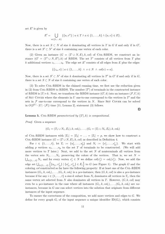
set E′ is given by

E′ =⋃

a∈1,...,ku, va | u ∈ T ∧ a ∈ 1, . . . , k ∧ u, v ∈ E .

Now, there is a set S ⊂ N of size k dominating all vertices in T in G if and only if in G′,there is a set S′ ⊂ N ′ of size k containing one vertex of each color.

(2) Given an instance (G = (T ∪ N,E), k, col) of Col-RBDS, we construct an in-stance (G′ = (T ′ ∪ N,E′), k) of RBDS. The set T ′ consists of all vertices from T plusk additional vertices z1, . . . , zk. The edge set E′ consists of all edges from E plus the edges

za, v | a ∈ 1, . . . , k ∧ v ∈ N ∧ col(v) = a.

Now, there is a set S′ ⊂ N ′ of size k dominating all vertices in T ′ in G′ if and only if in G,there is a set S ⊂ N of size k containing one vertex of each color.

(3) To solve Col-RBDS in the claimed running time, we first use the reduction givenin (2) from Col-RBDS to RBDS. The number |T ′| of terminals in the constructed instanceof RBDS is |T |+k. Next, we transform the RBDS instance (G′, k) into an instance (F , U, k)of Set Cover where the elements in U one-to-one correspond to the vertices in T ′ and thesets in F one-to-one correspond to the vertices in N . Since Set Cover can be solvedin O(2|U | · |U | · |F|) time [11, Lemma 2], statement (3) follows.

Lemma 5. Col-RBDS parameterized by (|T |, k) is compositional.

Proof. Given a sequence

(G1 = (T1 ∪N1, E1), k, col1), . . . , (Gt = (Tt ∪Nt, Et), k, colt)

of Col-RBDS instances with |T1| = |T2| = . . . = |Tt| = p, we show how to construct aCol-RBDS instance (G = (T ∪N,E), k, col) as described in Definition 4.

For i ∈ 1, . . . , t, let Ti := ui1, . . . , u

ip and Ni := vi

1, . . . , viqi. We start with

adding p vertices u1, . . . , up to the set T of terminals to be constructed. (We will addmore vertices to T later.) Next, we add to the set N of nonterminals all vertices fromthe vertex sets N1, . . . , Nt, preserving the colors of the vertices. That is, we set N =⋃

i∈1,...,t Ni, and for every vertex vij ∈ N we define col(vi

j) = coli(vij). Now, we add the

edge set⋃

i∈1,...,tuj1 , v

ij2 | ui

j1, vi

j2 ∈ Ei

to G (see Figure 1). The graph G and the

coloring col constructed so far have the following property: If at least one of the Col-RBDS

instances (G1, k, col1), . . . , (Gt, k, colt) is a yes-instance, then (G, k, col) is also a yes-instancebecause if for any i ∈ 1, . . . , t a size-k subset from Ni dominates all vertices in Ti, then thesame vertex set selected from N also dominates all vertices in T . However, (G, k, col) mayeven be a yes-instance in the case where all instances (G1, k, col1), . . . , (Gt, k, colt) are no-instances, because in G one can select vertices into the solution that originate from differentinstances of the input sequence.

To ensure the correctness of the composition, we add more vertices and edges to G. Wedefine for every graph Gi of the input sequence a unique identifier ID(Gi), which consists

11

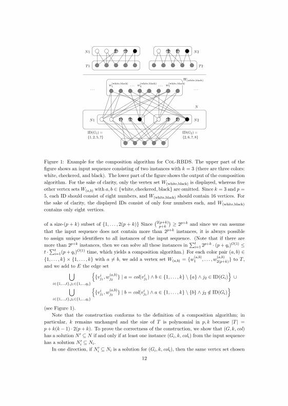
N1

N1

T 1

N2

N2

T 2

W(white,black)

. . .. . .w

(white,black)1 . . . w

(white,black)4 . . . w

(white,black)7

ID(G1) =1, 2, 5, 7

ID(G2) =2, 6, 7, 8

N

Figure 1: Example for the composition algorithm for Col-RBDS. The upper part of thefigure shows an input sequence consisting of two instances with k = 3 (there are three colors:white, checkered, and black). The lower part of the figure shows the output of the compositionalgorithm. For the sake of clarity, only the vertex set W(white,black) is displayed, whereas fiveother vertex sets W(a,b) with a, b ∈ white, checkered,black are omitted. Since k = 3 and p =5, each ID should consist of eight numbers, and W(white,black) should contain 16 vertices. Forthe sake of clarity, the displayed IDs consist of only four numbers each, and W(white,black)

contains only eight vertices.

of a size-(p + k) subset of 1, . . . , 2(p + k) Since(2(p+k)

p+k

) ≥ 2p+k and since we can assumethat the input sequence does not contain more than 2p+k instances, it is always possibleto assign unique identifiers to all instances of the input sequence. (Note that if there aremore than 2p+k instances, then we can solve all these instances in

∑ti=1 2p+k · (p + qi)O(1) ≤

t ·∑ti=1(p + qi)O(1) time, which yields a composition algorithm.) For each color pair (a, b) ∈

1, . . . , k × 1, . . . , k with a 6= b, we add a vertex set W(a,b) = w(a,b)1 , . . . , w

(a,b)2(p+k) to T ,

and we add to E the edge set⋃i∈1,...,t,j1∈1,...,qi

vi

j1 , w(a,b)j2

| a = col(vij1) ∧ b ∈ 1, . . . , k \ a ∧ j2 ∈ ID(Gi)

∪

⋃i∈1,...,t,j1∈1,...,qi

vi

j1 , w(a,b)j2

| b = col(vij1) ∧ a ∈ 1, . . . , k \ b ∧ j2 /∈ ID(Gi)

(see Figure 1).

Note that the construction conforms to the definition of a composition algorithm; inparticular, k remains unchanged and the size of T is polynomial in p, k because |T | =p + k(k− 1) · 2(p + k). To prove the correctness of the construction, we show that (G, k, col)has a solution N ′ ⊆ N if and only if at least one instance (Gi, k, coli) from the input sequencehas a solution N ′

i ⊆ Ni.In one direction, if N ′

i ⊆ Ni is a solution for (Gi, k, coli), then the same vertex set chosen

12

from N forms a solution for (G, k, col). To see this, first note that the vertices from T

are dominated by the chosen vertices. Moreover, for every color pair (a, b) ∈ 1, . . . , k ×1, . . . , k with a 6= b, each vertex from W(a,b) is either connected to all vertices v from Ni

with col(v) = a or to all vertices v from Ni with col(v) = b. Since N ′i contains one vertex of

each color class from Ni, each vertex in W(a,b) is dominated by a vertex from N chosen intothe solution.

In the other direction, to show that any solution N ′ ⊆ N for (G, k, col) is a solutionfor at least one instance (Gi, k, coli), we prove that N ′ cannot contain vertices originatingfrom different instances of the input sequence. To this end, note that each two verticesin N ′ must have different colors. Assume, for the sake of a contradiction, that N ′ containsa vertex vi1

j1with col(vi1

j1) = a originating from the instance (Gi1 , k, coli1) and a vertex vi2

j2

with col(vi2j2

) = b originating from a different instance (Gi2 , k, coli2). Due to the constructionof the IDs, we have ID(Gi1)\ ID(Gi2) 6= ∅ and ID(Gi2)\ ID(Gi1) 6= ∅. This implies that thereare vertices in W(a,b) (namely, all vertices w

(a,b)j with j ∈ ID(Gi2) \ ID(Gi1)) and vertices

in W(b,a) (namely, all vertices w(b,a)j with j ∈ ID(Gi1) \ ID(Gi2)) that are neither adjacent

to vi1j1

nor to vi2j2

. Therefore, N ′ does not dominate all vertices from T , which is a contradictionto the fact that N ′ is a solution for (G, k, col).

Theorem 8. ([8]) Red-Blue Dominating Set and Steiner Tree, both parameterizedby (|T |, k), Connected Vertex Cover and Capacitated Vertex Cover, both param-eterized by k, and Bounded Rank Set Cover, parameterized by (k, d), do not admitpolynomial kernels unless PH = Σ3

p.

Proof. For RBDS the statement of the theorem follows directly by Theorem 5 together withLemmata 4 and 5.

To show that the statement is true for the other four problems, we give polynomialparameter transformations from RBDS to each of them—due to Proposition 1, this sufficesto prove the statement. Let (G = (T ∪ N,E), k) be an instance of RBDS. To transform itinto an instance (G′ = (T ′ ∪ N,E′), k) of Steiner Tree, define T ′ = T ∪ u where u isa new vertex and let E′ = E ∪ u, vi | vi ∈ N. It is easy to see that every solution forSteiner Tree on (G′, k) one-to-one corresponds to a solution for RBDS on (G, k).

To transform (G, k) into an instance (G′′ = (V ′′, E′′), k′′) of ConVC, first construct thegraph G′ = (T ′ ∪ N,E′) as described above. The graph G′′ is then obtained from G′ byattaching a leaf to every vertex in T ′. Now, G′′ has a connected vertex cover of size k′′ =|T ′| + k = |T | + 1 + k iff G′ has a steiner tree containing k vertices from N iff all verticesfrom T can be dominated in G by k vertices from N .

Next, we describe how to transform (G, k) into an instance (G′′′ = (V ′′′, E′′′), cap, k′′′)of CapVC. First, for each vertex ui ∈ T , add a clique to G′′′ that contains four ver-tices u0

i , u1i , u

2i , u

3i . Second, for each vertex vi ∈ N , add a vertex v′′′i to G′′′. Finally, for

each edge ui, vj ∈ E with ui ∈ T and vj ∈ N , add the edge u0i , v

′′′j to G′′′. The capacities

of the vertices are defined as follows: For each vertex ui ∈ T , the vertices u1i , u

2i , u

3i ∈ V ′′′

have capacity 1 and the vertex u0i ∈ V ′′′ has capacity degG′′′(u0

i ) − 1. Each vertex v′′′i hascapacity degG′′′(v′′′i ). Clearly, in order to cover the edges of the size-4 cliques inserted for thevertices of T , every capacitated vertex cover for G′′′ must contain all vertices u0

i , u1i , u

2i , u

3i .

Moreover, since the capacity of each vertex u0i is too small to cover all edges incident to u0

i ,

13

at least one neighbor v′′′j of u0i must be selected into every capacitated vertex cover for G′′′.

Therefore, it is not hard to see that G′′′ has a capacitated vertex cover of size k′′′ = 4 · |T |+k

iff all vertices from T can be dominated in G by k vertices from N .Finally, to transform (G, k) into an instance (F , U, k) of Bounded Rank Set Cover,

add one element ei to U for every vertex ui ∈ T . For every vertex vj ∈ N , add one set ei |ui, vj ∈ E to F . The correctness of the construction is obvious, and since |U | = |T |, everyset in F contains at most d = |T | elements.

References

[1] Jochen Alber, Michael R. Fellows, and Rolf Niedermeier. Polynomial-time data reduc-tion for dominating set. J. ACM, 51(3):363–384, 2004.

[2] Noga Alon, Raphael Yuster, and Uri Zwick. Color-coding. J. Assoc. Comput. Mach.,42(4):844–856, 1995.

[3] Hans L. Bodlaender, Rodney G. Downey, Michael R. Fellows, and Danny Hermelin. Onproblems without polynomial kernels. In Proc. 35th ICALP, volume 5125 of LNCS,pages 563–574. Springer, 2008.

[4] Hans L. Bodlaender, Stephan Thomasse, and Anders Yeo. Analysis of data reduction:Transformations give evidence for non-existence of polynomial kernels. Technical Re-port UU-CS-2008-030, Department of Information and Computing Sciences, UtrechtUniversity, 2008.

[5] Jianer Chen, Henning Fernau, Iyad A. Kanj, and Ge Xia. Parametric duality andkernelization: Lower bounds and upper bounds on kernel size. In Proc. 22nd STACS,volume 3404 of LNCS, pages 269–280. Springer, 2005.

[6] Jianer Chen, Iyad A. Kanj, and Weijia Jia. Vertex Cover: Further observations andfurther improvements. J. Algorithms, 41(2):280–301, 2001.

[7] Benny Chor, Mike Fellows, and David W. Juedes. Linear kernels in linear time, or howto save k colors in o(n2) steps. In Proc. 30th WG, volume 3353 of LNCS, pages 257–269.Springer, 2004.

[8] Michael Dom, Daniel Lokshtanov, and Saket Saurabh. Incompressibility through Colorsand IDs. In Proc. 36th ICALP, To appear.

[9] Henning Fernau, Fedor V. Fomin, Daniel Lokshtanov, Daniel Raible, Saket Saurabh,and Yngve Villanger. Kernel(s) for problems with no kernel: On out-trees with manyleaves. In Proc. 26th STACS, pages 421–432.

[10] J. Flum and M. Grohe. Parameterized Complexity Theory (Texts in Theoretical Com-puter Science. An EATCS Series). Springer-Verlag New York, Inc., Secaucus, NJ, USA,2006.

14

[11] Fedor V. Fomin, Dieter Kratsch, and Gerhard J. Woeginger. Exact (exponential) algo-rithms for the dominating set problem. In Proc. 30th WG, volume 3353 of LNCS, pages245–256. Springer, 2004.

[12] Lance Fortnow and Rahul Santhanam. Infeasibility of instance compression and succinctPCPs for NP. In Proc. 40th STOC, pages 133–142. ACM Press, 2008.

[13] Michael R. Garey and David S. Johnson. Computers and Intractability: A Guide to theTheory of NP-Completeness. Freeman, 1979.

[14] J. Gramm, J. Guo, F. Huffner, and R. Niedermeier. Data reduction, exact, and heuristicalgorithms for Clique Cover. In Proc. 8th ACM-SIAM ALENEX, pages 86–94. ACM-SIAM, 2006. Long version to appear in The ACM Journal of Experimental Algorithmics.

[15] Rolf Niedermeier. An Invitation to Fixed-Parameter Algorithms. Oxford UniversityPress, 2006.

[16] W. V. Quine. The problem of simplifying truth functions. Amer. Math. Monthly,59:521–531, 1952.

[17] Larry J. Stockmeyer. The polynomial-time hierarchy. Theor. Comput. Sci., 3(1):1–22,1976.

[18] Stephan Thomasse. A quadratic kernel for feedback vertex set. In Proc. 20th SODA,pages 115–119. ACM/SIAM, 2009.

15