Aggregate Risk and the Choice between Cash and Lines · PDF fileAggregate Risk and the Choice between Cash and Lines of Credit VIRAL V. ACHARYA, HEITOR ALMEIDA, and, MURILLO CAMPELLO

Aggregate Risk and the Choice between Cash and Lines of Credit

VIRAL V. ACHARYA, HEITOR ALMEIDA, and, MURILLO CAMPELLO *

First draft: September 2009; This draft: June 2012

Abstract

We model corporate liquidity policy and show that aggregate risk exposure is a key determinant ofhow firms choose between cash and bank credit lines. Banks create liquidity for firms by pooling theiridiosyncratic risks. As a result, firms with high aggregate risk find it costly to get credit lines and optfor cash in spite of higher opportunity costs and liquidity premium. Likewise, in times when aggregaterisk is high, firms rely more on cash than on credit lines. We verify these predictions empirically.Cross-sectional analyses show that firms with high exposure to systematic risk have a higher ratio ofcash to credit lines and face higher costs on their lines. Time-series analyses show that firms’ cashreserves rise in times of high aggregate volatility and in such times credit lines initiations fall, theirspreads widen, and maturities shorten. Also consistent with the mechanism in the model, we find thatexposure to undrawn credit lines increases bank-specific risks in times of high aggregate volatility.

Key words: Bank lines of credit, cash holdings, liquidity management, systematic risk, loan spreads, loan

maturity, asset beta.

JEL classification: G21, G31, G32, E22, E5.

*Viral V. Acharya is with NYU-Stern, CEPR, ECGI, and NBER. Heitor Almeida is with University of Illinois,and NBER. Murillo Campello is with Cornell University, and NBER. Our paper benefited from comments from

Peter Tufano (editor), an anonymous referee, Hui Chen, Ran Duchin and Robert McDonald (discussants), and

Rene Stulz, as well as seminar participants at the 2010 AEA meetings, 2010 WFA meetings, DePaul University,

ESSEC, Emory University, MIT, Moody’s/NYU Stern 2010 Credit Risk Conference, New York University,

Northwestern University, UCLA, University of Illinois, Vienna University of Economics and Business, Yale

University, University of Southern California and UCSD. We thank Florin Vasvari and Anurag Gupta for

help with the data on lines of credit, and Michael Roberts and Florin Vasvari for matching these data with

COMPUSTAT. Farhang Farazmand, Fabrício D’Almeida, Igor Cunha, Rustom Irani, Hanh Le, Ping Liu, and

Quoc Nguyen provided excellent research assistance. We are also grateful to Jaewon Choi for sharing his data

on firm betas, and to Thomas Philippon and Ran Duchin for sharing their programs to compute asset and

financing gap betas.

Aggregate Risk and the Choice between Cash and Lines of Credit

Abstract

We model corporate liquidity policy and show that aggregate risk exposure is a key determinant ofhow firms choose between cash and bank credit lines. Banks create liquidity for firms by pooling theiridiosyncratic risks. As a result, firms with high aggregate risk find it costly to get credit lines and optfor cash in spite of higher opportunity costs and liquidity premium. Likewise, in times when aggregaterisk is high, firms rely more on cash than on credit lines. We verify these predictions empirically.Cross-sectional analyses show that firms with high exposure to systematic risk have a higher ratio ofcash to credit lines and face higher costs on their lines. Time-series analyses show that firms’ cashreserves rise in times of high aggregate volatility and in such times credit lines initiations fall, theirspreads widen, and maturities shorten. Also consistent with the mechanism in the model, we find thatexposure to undrawn credit lines increases bank-specific risks in times of high aggregate volatility.




“A Federal Reserve survey earlier this year found that about one-third of U.S. banks have tightened their

standards on loans they make to businesses of all sizes. And about 45% of banks told the Fed that they are

charging more for credit lines to large and midsize companies. Banks such as Citigroup Inc., which has been

battered by billions of dollars in write-downs and other losses, are especially likely to play hardball, resisting

pleas for more credit or pushing borrowers to pay more for loan modifications.”

– The Wall Street Journal, March 8, 2008

How do firms manage their liquidity needs? This question has become increasingly important for

both academic research and corporate finance in practice. Survey evidence indicates that liquidity

management tools such as cash and credit lines are essential components of a firm’s financial pol-

icy (see Lins, Servaes, and Tufano (2010) and Campello, Giambona, Graham, and Harvey (2010)).

Consistent with the evidence from surveys, a number of studies show that the funding of invest-

ment opportunities is a key determinant of corporate cash policy (e.g., Opler, Pinkowitz, Stulz, and

Williamson (1999), Almeida, Campello, and Weisbach (2004, 2009), and Duchin (2009)). Recent

work also shows that bank lines of credit have become an important source of firm financing (Sufi

(2009), Disatnik, Duchin, and Schmidt (2010)). The evidence further suggests that credit lines

played a crucial role in the liquidity management of firms during the recent credit crisis (Ivashina

and Scharfstein (2010)).

In contrast to the growing empirical literature, there is limited theoretical work on the rea-

sons why firms may use “pre-committed” sources of funds (such as cash or credit lines) to manage

1

their liquidity needs. In principle, a firm can use other sources of funding for long-term liquidity

management, such as future operating cash flows or proceeds from debt issuances. However, these

alternatives expose the firm to additional risks because their availability depends on firm perfor-

mance. Holmstrom and Tirole (1997, 1998), for example, show that relying on future issuance of

external claims is insufficient to provide liquidity for firms that face costly external financing. Simi-

larly, Acharya, Almeida, and Campello (2007) show that cash holdings dominate spare debt capacity

for financially constrained firms that have their financing needs concentrated in states of the world

where cash flows are low. Notably, these models of liquidity insurance are silent on the trade-offs

between cash and credit lines.1

This paper attempts to fill this gap in the liquidity management literature. Building on Holm-

strom and Tirole (1998) and Tirole (2006), we develop a model of the trade-offs firms face when

choosing between holding cash and securing a credit line. The key insight of our argument is that a

firm’s exposure to aggregate risks – its “beta” – is a fundamental determinant of liquidity choices.

The intuition is straightforward. In the presence of a liquidity premium (e.g., a low return on cash

holdings), firms find it costly to hold cash. Firms may instead manage their liquidity needs using

bank credit lines, which do not require them to hold liquid assets. Under a credit line agreement,

the bank provides the firm with funds when the firm faces a liquidity shortfall. In exchange, the

bank collects payments from the firm in states of the world in which the firm does not need the

funds under the line (e.g., commitment fees). The credit line can thus be seen as an insurance

contract. Provided that the bank can offer this insurance at “actuarially fair” terms, lines of credit

will dominate cash holdings in corporate liquidity management.

The drawback of credit lines, however, is that banks may not be able to provide liquidity in-

surance for all firms in the economy at all times. Consider, for example, a situation in which a

large fraction of the corporate sector is hit by a liquidity shock. In this state of the world, banks

might become unable to guarantee liquidity since the demand for funds under the outstanding lines

(drawdowns) may exceed the supply of funds coming from healthy firms. In other words, the ability

of the banking sector to meet corporate liquidity needs depends on the extent to which firms are

subject to correlated (systematic) liquidity shocks. Aggregate risk thus creates a cost to credit lines.

We explore this trade-off between aggregate risk and liquidity premia to derive optimal corporate

liquidity policy. We do this in an equilibrium model in which firms are heterogeneous with respect

to their exposure to aggregate risks (firms have different betas). We show that while low beta firms

manage their liquidity through bank credit lines, high beta firms optimally choose to hold cash,

despite the liquidity premium. Because the banking sector manages primarily idiosyncratic risk, it

1A recent paper by Bolton, Chen, and Wang (2011) introduces both cash and credit lines in a dynamic investment

framework with costly external finance. In their model, the size of the credit line facility is given exogenously, thus

they do not analyze the ex-ante trade-off between cash and credit lines (see also DeMarzo and Fishman (2007)).

2

can provide liquidity for low beta firms even in bad states of the world. In equilibrium, low beta

firms therefore face better contractual terms when initiating credit lines, demand more lines, and

hold less cash in equilibrium. On the flip side, high beta firms face worse contractual terms, demand

less lines, and hold more cash. This logic suggests that firms’ exposure to systematic risks increases

the demand for cash and reduces the demand for credit lines. In a similar fashion, when there is an

increase in aggregate risk there is greater aggregate reliance on cash relative to credit lines.

In addition to this basic result, the model generates a number of insights on liquidity manage-

ment. These, in turn, motivate our empirical analysis. First, the model suggests that exposure to

risks that are systematic to the banking industry should affect corporate liquidity policy. In par-

ticular, firms that are more sensitive to banking industry downturns should be more likely to hold

cash for liquidity management. Second, the trade-off between cash and credit lines should be more

important for firms that find it more costly to raise external capital. Third, the effect of aggregate

risk exposure on liquidity policy should be stronger for firms that have high aggregate risk, as these

firms have the strongest impact on bank liquidity constraints. Fourth, lines of credit should be more

expensive for firms with greater aggregate risk and in times of higher aggregate volatility.

We test these cross-sectional and time-series implications using data from the 1987—2008 pe-

riod.2 For the cross-sectional analysis, we use two alternative data sources to construct proxies for

the availability of credit lines. Our first sample is drawn from the LPC-DealScan database. These

data allow us to construct a large sample of credit line initiations. The LPC-DealScan data, however,

have two limitations. First, they are largely based on syndicated loans, thus biased towards large

deals (consequently large firms). Second, they do not reveal the extent to which existing lines have

been used (drawdowns). To overcome these issues, we also use an alternative sample that contains

detailed information on the credit lines initiated and used by a random sample of 300 firms between

1996 and 2003. These data are drawn from Sufi (2009). Using both LPC-DealScan and Sufi’s data

sets, we measure the fraction of corporate liquidity that is provided by lines of credit as the ratio of

total credit lines to the sum of total credit lines plus cash. For short, we call this variable LC-to-Cash

ratio. While some firms may have higher demand for total liquidity due to variables such as better

investment opportunities, the LC-to-Cash ratio isolates the relative usage of lines of credit versus

cash in corporate liquidity management.

Our main hypothesis is that a firm’s exposure to aggregate risk should be negatively related to

its LC-to-Cash ratio. In the model, the relevant aggregate risk is the correlation of a firm’s financing

needs with those of other firms in the economy. While this could suggest using a “cash flow beta,”

note that cash flow-based measures are slow-moving and available only at low frequency. Under the

2To be precise, we use a panel dataset to test the model’s cross-sectional implications. However most of the

variation in our proxies for firm-level systematic risk exposure is cross-sectional in nature.

3

assumption that a firm’s financing needs go up when its stock return falls, the relevant beta is the

traditional beta of the firm with respect to the overall stock market. Accordingly, we employ a stan-

dard stock market-based beta as our baseline measure of risk exposure. For robustness, however, we

also use cash flow-based betas.3 To test the prediction that a firm’s exposure to banking sector’s risk

should influence the firm’s liquidity policy, we measure “bank beta” as the beta of a firm’s returns

with respect to the banking sector aggregate return.

Our market-based measures of beta are asset (i.e., unlevered) betas. While equity betas are easy

to compute using stock price data, they are mechanically related to leverage (high leverage firms

will tend to have larger betas). Since greater reliance on credit lines will typically increase the firm’s

leverage, the “mechanical” leverage effect may bias our estimates. To overcome this problem, we

unlever equity betas by using a Merton-KMV-type model for firm value, or alternatively we compute

betas using data on firm asset returns (from Choi (2009)). We also tease out the relative importance

of systematic and idiosyncratic risk for corporate liquidity policy, by decomposing total asset risk

on its systematic and idiosyncratic components.

We test the theory’s cross-sectional implications by relating systematic risk exposure to LC-to-

Cash ratios. In a nutshell, all of our tests lead to a similar conclusion: exposure to systematic risk

has a statistically and economically significant impact on the fraction of corporate liquidity that is

provided by credit lines. Using the LPC-DealScan sample, for example, we find that an increase in

beta from 0.8 to 1.5 (this is less than a one-standard deviation change in beta) decreases a firm’s

reliance on credit lines by 0.06 (approximately 15% of the standard deviation and 20% of the sample

average value of LC-to-Cash). We also find that the systematic component of asset variance has a

negative and significant effect on the LC-to-Cash ratio. These findings support our theory’s predic-

tions. Notably, the inferences we draw hold across both the larger LPC-DealScan dataset and the

smaller, more detailed data constructed by Sufi (both for total and unused credit lines).

The negative relation between systematic risk exposure and LC-to-Cash holds for all different

proxies of betas that we employ, including Choi’s (2009) asset-return based betas, betas that are

unlevered using net rather than gross debt (to account for a possible effect of cash on asset betas),

equity (levered) betas, and cash flow-based betas. The results also hold for “bank betas” (suggesting

that firms that are more sensitive to banking industry downturns are more likely to hold cash for

liquidity management) and “tail betas” (suggesting that a firm’s sensitivity to market downturns af-

fects corporate liquidity policy). These estimates agree with our theory and imply a strong economic

relation between exposure to aggregate risk and liquidity management.

In additional tests, we sort firms according to observable proxies of financing constraints to study

3In addition, we employ a “tail beta” that uses data from the days with the worst returns in the year to compute beta

(cf. Acharya, Pedersen, Philippon, and Richardson (2010)). This beta proxy captures the idea that a firm’s exposure

to systematic risks matters mostly on the downside (because a firm may need liquidity when other firms face problems).

4

whether the effect of beta on LC-to-Cash is driven by firms that are likely to be constrained. As

predicted by our model, the relation between beta and the use of credit lines only holds in samples

of likely constrained firms (e.g., across small and low payout firms). When we sort firms in “high

beta” and “low beta” groups, we find that the effect of beta on the LC-to-Cash ratio is significantly

stronger in the sample of high beta firms (consistent with our story). Finally, we study the relation

between firms’ beta and the fees and spreads that they commit to pay on bank lines of credit. We

find that high beta firms pay significantly higher fees on their undrawn balances, and also higher

spreads when drawing on their credit lines. This is direct evidence that it is more costly for banks

to provide liquidity insurance for aggregate risky firms.

Next, we examine our model’s time-series implications. These tests gauge aggregate risk using

VIX, the implied volatility of the stock market index returns from options data. VIX captures

both aggregate volatility as well as the financial sector’s appetite to bear that risk. In addition,

we examine whether expected volatility in the banking sector drives time-series variation in corpo-

rate liquidity policy. Given limited historical data on implied volatility for the banking sector, we

construct Bank VIX, the expected banking sector volatility, using a GARCH model.

Controlling for real GDP growth and flight-to-quality effects (see Gatev and Strahan (2005)), we

find that an increase in VIX and/or Bank VIX reduces credit line initiations and raises firms’ cash

reserves (Figure 4 provides a visual illustration). The maturity of credit lines shrinks as aggregate

volatility rises, and new credit lines become more expensive in those times (see Figure 5). We confirm

that these effects are not due to an overall increase in the cost of debt by showing that firms’ debt

issuances are not affected by VIX. In other words, the negative impact of VIX on new debt operates

through availability of lines of credit. These results point out that an increase in aggregate risk in

the economy is an important limitation of bank-provided liquidity insurance to firms.

Finally, we provide evidence for the mechanism that drives corporate liquidity choices in our

model. The model suggests that an increase in aggregate risk in the economy creates liquidity risk

for banks that are exposed to undrawn corporate credit lines. Thus, banks increase the cost of

credit lines for aggregate risky firms, which in turn move towards cash holdings. Nevertheless, a

possible alternative interpretation for the results is related to the risk of covenant violations (as in

Sufi (2009)). For example, if firms are more likely to violate covenants in times when aggregate risk

is high, then “high beta” firms may move to cash holdings not because of banks’ liquidity constraint

as in our model, but because of the risk of covenant violations.

In order to disentangle these two stories, we devise a direct test of the prediction that aggregate

risk exposure tightens banks’ liquidity constraints through a credit line channel. The link between

credit line exposure and bank risk has been studied by Gatev, Schuermann, and Strahan (2009).

They find that bank risk, as measured by stock return volatility, increases with unused credit lines

5

that the bank has agreed to extend to the corporate sector. The mechanism in our model would

then suggest that the impact of credit line exposure on bank risk should increase during periods

of high aggregate risk. We test and confirm this prediction using bank-level data (taken from “call

reports”). In addition, we examine the hypothesis that covenant violations (or credit line revocations

conditional on violations) increase during periods of high aggregate volatility (or for firms with high

aggregate risk exposure). Our results suggest that aggregate risk does not increase the sensitivity

of covenant violations to profitability shocks. In addition, the effect of covenant violations on credit

line revocations is largely independent of firms’ aggregate risk exposures.4 These results provide

additional evidence that the link between liquidity management and aggregate risk uncovered in our

tests indeed due to the effect of aggregate risk on banks’ liquidity constraints.

Our work has connections with recent literature that discusses firms’ liquidity choices and it is

important that we highlight our contributions. Relative to Sufi (2009), our contribution is to show

that the (largely idiosyncratic) risk of covenant violations is not the only type of risk that affects

firms’ choice between cash and credit lines. Firms’ exposure to aggregate risk, and the ensuing ef-

fects on banks’ liquidity constraints are also key forces that drive corporate liquidity policy. Relative

to the growing new literature on firms’ choices between credit lines and cash (e.g., Lins, Servaes,

and Tufano (2010), Campello, Giambona, Graham, and Harvey (2010), and Disatnik, Duchin, and

Schmidt (2010)), we are the first to advance and test a full-fledged theory explaining how corporate

exposure to aggregate risk drives their liquidity management. We also provide a novel assessment of

the importance of financial intermediary risk to the choice between cash and lines. In fact, papers in

the cash—credit line choice generally abstract from connections between the macroeconomy, banks,

and firms when examining liquidity management.5 We believe our paper represents a step forward in

establishing a theoretical framework describing these connections and in showing how they operate.

Understanding and characterizing these links should be of interest for future research, especially

around important episodes such as financial crises.

The paper is organized as follows. In the next section, we develop our model and derive its empir-

ical implications. We present the empirical tests in Section II.. Section III. offers concluding remarks.

I. Model

Our model is based on Holmstrom and Tirole (1998) and Tirole (2006), who consider the role

of aggregate risk in affecting corporate liquidity policy. We introduce firm heterogeneity in their

4Since a credit line is a loan commitment, it may not be easy for the bank to revoke access to the line once it is

initiated. In order for the bank to revoke access, the firm must be in violation of a covenant. Given that covenant

violations are unrelated to systematic risk after controlling for firm profitability (as the evidence in this paper suggests),

banks do not revoke access simply because aggregate risk is high.5Exceptions are papers written on the 2008-9 crisis, such as Campello, Giambona, Graham, and Harvey (2010)

and Ivashina and Scharfstein (2010).

6

framework to analyze the trade-offs between cash and credit lines.

The economy has a unit mass of firms. Each firm has access to an investment project that requires

fixed investment I at date 0. The investment opportunity also requires an additional investment at

date 1, of uncertain size. This additional investment represents the firms’ liquidity need at date 1. We

assume that the date-1 investment need can be either equal to ρ, with probability λ, or 0, with prob-

ability (1−λ). There is no discounting and everyone is risk-neutral, so that the discount factor is one.Firms are symmetric in all aspects, with one important exception. They differ in the extent to

which their liquidity shocks are correlated with each other. A fraction θ of the firms has perfectly

correlated liquidity shocks; that is, they all either have a date-1 investment need, or not. We call

these firms systematic firms. The other fraction of firms (1− θ) has independent investment needs;

that is, the probability that a firm needs ρ is independent of whether other firms need ρ or 0. These

are the non-systematic firms. We can think of this set up as one in which an aggregate state realizes

first. The realized state then determines whether or not systematic firms have liquidity shocks.

We refer to states as follows. We let the aggregate state in which systematic firms have a liquidity

shock be denoted by λθ. Similarly, (1− λθ) is the state in which systematic firms have no liquidity

demand. After the realization of this aggregate state, non-systematic firms learn whether they have

liquidity shocks. The state in which non-systematic firms do get a shock is denoted as λ and the

other state as (1−λ). Note that the likelihood of both λ and λθ states is λ. In other words, to avoidadditional notation, we denote states by their probability, but single out the state in which systematic

firms are all hit by a liquidity shock with the superscript θ. The set up is summarized in Figure 1.

− Figure 1 about here −

A firm will only continue its date-0 investment until date 2 if it can meet the date-1 liquidity

need. If the liquidity need is not met, then the firm is liquidated and the project produces a cash

flow equal to zero. If the firm continues, the investment produces a date-2 cash flow R which obtains

with probability p. With probability 1 − p, the investment produces nothing. The probability ofsuccess depends on the input of specific human capital by the firms’ managers. If the managers

exert high effort, the probability of success is equal to pG. Otherwise, the probability is pB, but the

managers consume a private benefit equal to B. While the cash flow R is verifiable, the managerial

effort and the private benefit are not verifiable and contractible. Because of the moral hazard due

this private benefit, managers must keep a high enough stake in the project to be induced to exert

effort. We assume that the investment is negative NPV if the managers do not exert effort, implying

the following incentive constraint: pGRM ≥ pBRM + B, or RM ≥ B∆p, where RM is the managers’

compensation and ∆p = pG − pB. This moral hazard problem implies that the firms’ cash flows

7

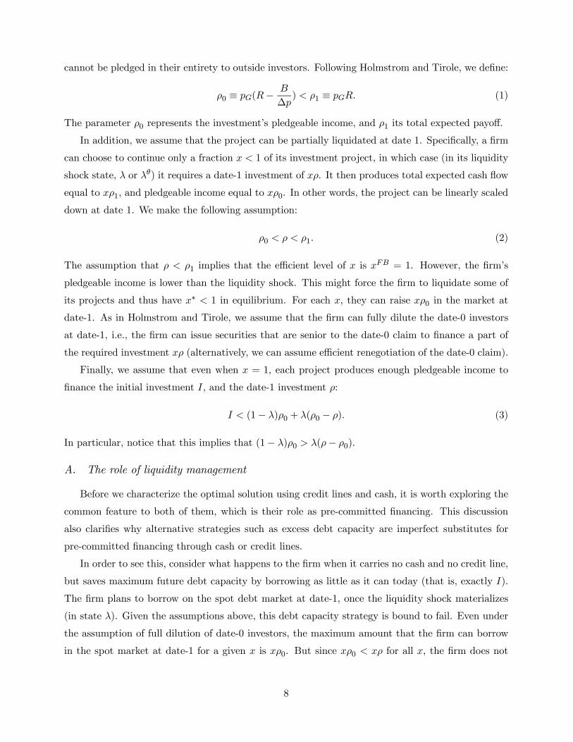
cannot be pledged in their entirety to outside investors. Following Holmstrom and Tirole, we define:

ρ0 ≡ pG(R−B

∆p) < ρ1 ≡ pGR. (1)

The parameter ρ0 represents the investment’s pledgeable income, and ρ1 its total expected payoff.

In addition, we assume that the project can be partially liquidated at date 1. Specifically, a firm

can choose to continue only a fraction x < 1 of its investment project, in which case (in its liquidity

shock state, λ or λθ) it requires a date-1 investment of xρ. It then produces total expected cash flow

equal to xρ1, and pledgeable income equal to xρ0. In other words, the project can be linearly scaled

down at date 1. We make the following assumption:

ρ0 < ρ < ρ1. (2)

The assumption that ρ < ρ1 implies that the efficient level of x is xFB = 1. However, the firm’s

pledgeable income is lower than the liquidity shock. This might force the firm to liquidate some of

its projects and thus have x∗ < 1 in equilibrium. For each x, they can raise xρ0 in the market at

date-1. As in Holmstrom and Tirole, we assume that the firm can fully dilute the date-0 investors

at date-1, i.e., the firm can issue securities that are senior to the date-0 claim to finance a part of

the required investment xρ (alternatively, we can assume efficient renegotiation of the date-0 claim).

Finally, we assume that even when x = 1, each project produces enough pledgeable income to

finance the initial investment I, and the date-1 investment ρ:

I < (1− λ)ρ0 + λ(ρ0 − ρ). (3)

In particular, notice that this implies that (1− λ)ρ0 > λ(ρ− ρ0).

A. The role of liquidity management

Before we characterize the optimal solution using credit lines and cash, it is worth exploring the

common feature to both of them, which is their role as pre-committed financing. This discussion

also clarifies why alternative strategies such as excess debt capacity are imperfect substitutes for

pre-committed financing through cash or credit lines.

In order to see this, consider what happens to the firm when it carries no cash and no credit line,

but saves maximum future debt capacity by borrowing as little as it can today (that is, exactly I).

The firm plans to borrow on the spot debt market at date-1, once the liquidity shock materializes

(in state λ). Given the assumptions above, this debt capacity strategy is bound to fail. Even under

the assumption of full dilution of date-0 investors, the maximum amount that the firm can borrow

in the spot market at date-1 for a given x is xρ0. But since xρ0 < xρ for all x, the firm does not

8

have enough funds to pay for the liquidity shock, and must liquidate the project. In other words, in

the absence of cash and/or a credit line, x∗ = 0.

The problem with this “wait and see” strategy is that it does not generate enough debt capacity

in future liquidity states, while at the same time wasting debt capacity in states of the world with no

liquidity shock. Notice that in the no-liquidity-shock state (state 1− λ), the firm has debt capacity

equal to ρ0, but no required investments. In this context, the role of corporate liquidity policy (that

is, cash and credit lines) is to transfer financing capacity from the good to the bad state of the world.

The firm accomplishes this transfer using cash by borrowing more than I at date 0, and promising a

larger payment to investors in the good future state of the world, state 1−λ. The firm accomplishesthis transfer using credit lines by paying a commitment fee to banks in future good states of the

world, in exchange for the right to borrow in the bad state of the world. The difference between

standard debt issuance and a credit line is that the latter is pre-committed, while the former must

be contracted on the spot market (thus creating potential liquidity problems).

B. Solution using credit lines

We assume that the economy has a single, large intermediary who will manage liquidity for all

firms (“the bank”) by offering lines of credit. The credit line works as follows. The firm commits to

making a payment to the bank in states of the world in which liquidity is not needed. We denote

this payment (“commitment fee”) by y. In return, the bank commits to lending to the firm at a

pre-specified interest rate, up to a maximum limit. We denote the maximum size of the line by w.

In addition, the bank lends enough money (I) to the firms at date 0 so that they can start their

projects, in exchange for a promised date-2 debt payment D.

To fix ideas, let us imagine for now that firms have zero cash holdings. In the next section we

will allow firms to both hold cash, and also open bank credit lines.

In order for the credit line to allow firms to invest up to amount x in state λ, it must be that:

w(x) ≥ x(ρ− ρ0). (4)

In return, in state (1−λ), the financial intermediary can receive up to the firm’s pledgeable income,

either through the date-1 commitment fee y, or through the date-2 payment D. We thus have the

budget constraint:

y + pGD ≤ ρ0. (5)

The intermediary’s break even constraint is:

I + λx(ρ− ρ0) ≤ (1− λ)ρ0. (6)

9

Finally, the firm’s payoff is:

U(x) = (1− λ)ρ1 + λ(ρ1 − ρ)x− I. (7)

Given assumption (3), equation (6) will be satisfied by x = 1, and thus the credit line allows firms

to achieve the first-best investment policy.

The potential problem with the credit line is adequacy of bank liquidity. To provide liquidity for

the entire corporate sector, the intermediary must have enough available funds in all states of the

world. Since a fraction θ of firms will always demand liquidity in the same state, it is possible that

the intermediary will run out of funds in the bad aggregate state. In order to see this, notice that

in order obtain x = 1 in state λθ, the following inequality must be obeyed:

(1− θ)(1− λ)ρ0 ≥ [θ + (1− θ)λ] (ρ− ρ0). (8)

The left-hand side represents the total pledgeable income that the intermediary has in that state,

coming from the non-systematic firms that do not have liquidity needs. The right-hand side rep-

resents the economy’s total liquidity needs, from the systematic firms and from the fraction of

non-systematic firms that have liquidity needs. Clearly, from (3) there will be a θmax > 0, such that

this condition is met for all θ < θmax. This leads to an intuitive result:

PROPOSITION 1 The intermediary solution with lines of credit achieves the first-best investment

policy if and only if systematic risk is sufficiently low (θ < θmax), where θmax =ρ0−λρ(1−λ)ρ .

C. The choice between cash and credit lines

We now allow firms to hold both cash and open credit lines, and analyze the properties of the

equilibria that obtain for different parameter values. Analyzing this trade-off constitutes the most

important and novel theoretical contribution of our paper.

Firms’ optimization problem. To characterize the equilibria, we introduce some notation. We

let Lθ (alternatively, L1−θ) represent the cash demand by systematic (non-systematic) firms. Simi-

larly, xθ (x1−θ) represents the investment level that systematic (non-systematic) firms can achieve in

equilibrium. In addition, the credit line contracts that are offered by the bank can also differ across

firm types. That is, we assume that a firm’s type is observable by the bank at the time of contract-

ing. Thus, (Dθ, wθ, yθ) represents the contract offered to systematic firms, and (D1−θ, w1−θ, y1−θ)

represents the contract offered to non-systematic firms. For now, we assume that the bank cannot

itself carry cash and explain later why this is in fact the equilibrium outcome in the model.

As in Holmstrom and Tirole (1998), we assume that there is a supply Ls of a liquid and safe asset

(such as treasury bonds) that the firm can buy at date-0 and hold until date-1 to implement a given

10

cash policy L. This asset trades at a price equal to q at date 0. In the absence of a liquidity premium,

this safe asset should have a price equal to q = 1. The price q will be determined in equilibrium in

our model, and in some cases may be greater than one. If so, then holding cash is costly for the firm.

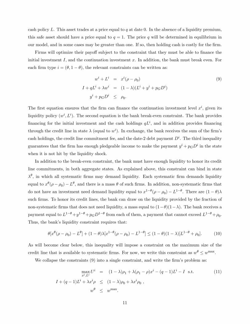
Firms will optimize their payoff subject to the constraint that they must be able to finance the

initial investment I, and the continuation investment x. In addition, the bank must break even. For

each firm type i = (θ, 1− θ), the relevant constraints can be written as:

wi + Li = xi(ρ− ρ0) (9)

I + qLi + λwi = (1− λ)(Li + yi + pGDi)

yi + pGDi ≤ ρ0.

The first equation ensures that the firm can finance the continuation investment level xi, given its

liquidity policy (wi, Li). The second equation is the bank break-even constraint. The bank provides

financing for the initial investment and the cash holdings qLi, and in addition provides financing

through the credit line in state λ (equal to wi). In exchange, the bank receives the sum of the firm’s

cash holdings, the credit line commitment fee, and the date-2 debt payment Di. The third inequality

guarantees that the firm has enough pledgeable income to make the payment yi+ pGDi in the state

when it is not hit by the liquidity shock.

In addition to the break-even constraint, the bank must have enough liquidity to honor its credit

line commitments, in both aggregate states. As explained above, this constraint can bind in state

λθ, in which all systematic firms may demand liquidity. Each systematic firm demands liquidity

equal to xθ(ρ− ρ0)−Lθ, and there is a mass θ of such firms. In addition, non-systematic firms thatdo not have an investment need demand liquidity equal to x1−θ(ρ− ρ0)− L1−θ. There are (1− θ)λ

such firms. To honor its credit lines, the bank can draw on the liquidity provided by the fraction of

non-systematic firms that does not need liquidity, a mass equal to (1−θ)(1−λ). The bank receives apayment equal to L1−θ+y1−θ+pGD1−θ from each of them, a payment that cannot exceed L1−θ+ρ0.

Thus, the bank’s liquidity constraint requires that:

θ[xθ(ρ− ρ0)− Lθ] + (1− θ)λ[x1−θ(ρ− ρ0)− L1−θ] ≤ (1− θ)(1− λ)[L1−θ + ρ0]. (10)

As will become clear below, this inequality will impose a constraint on the maximum size of the

credit line that is available to systematic firms. For now, we write this constraint as wθ ≤ wmax.We collapse the constraints (9) into a single constraint, and write the firm’s problem as:

maxxi,Li

U i = (1− λ)ρ1 + λ(ρ1 − ρ)xi − (q − 1)Li − I s.t. (11)

I + (q − 1)Li + λxiρ ≤ (1− λ)ρ0 + λxiρ0 ,

wθ ≤ wmax.

11

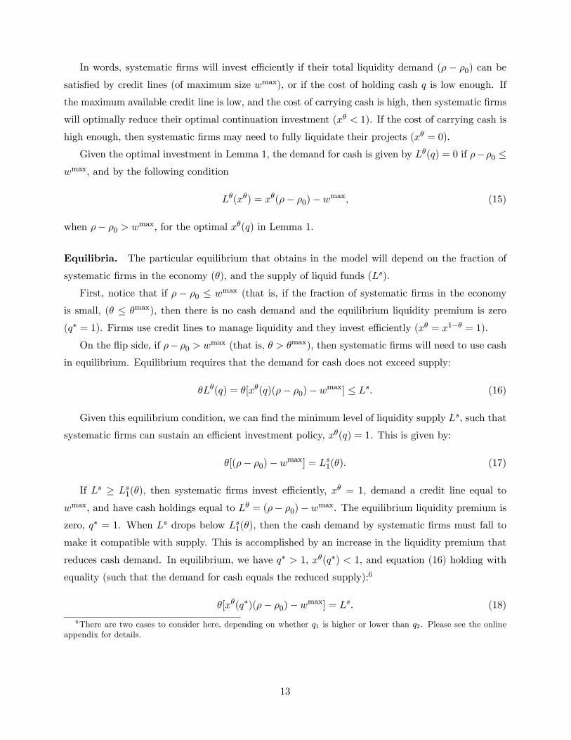
This problem determines firms’ optimal cash holdings and continuation investment, which are

a function of the liquidity premium, Li(q) and xi(q). In equilibrium, the total demand from cash

coming from systematic and non-systematic firms cannot exceed the supply of liquid funds:

θLθ(q) + (1− θ)L1−θ(q) ≤ Ls. (12)

This condition determines the cost of holding cash, q. We denote the equilibrium price by q∗.

Optimal firm policies. The first point to notice is that non-systematic firms will never find it

optimal to hold cash. In the optimization problem (11), firms’ payoffs decrease with cash holdings

Li if q∗ > 1, and they are independent of Li if q∗ = 1. Thus, the only situation in which a firm

might find it optimal to hold cash is when the constraint xθ(ρ − ρ0) − Lθ ≤ wmax is binding. Butthis constraint can only bind for systematic firms. Notice also that if Li = 0 the solution of the

optimization problem (11) is xi = 1 (the efficient investment policy). Thus, non-systematic firms

always invest optimally, x1−θ = 1.

Given that non-systematic firms use credit lines to manage liquidity and invest optimally, we can

rewrite constraint (10) as:

xθ(ρ− ρ0)− Lθ ≤ (1− θ)(ρ0 − λρ)

θ≡ wmax.

This expression gives the maximum size of the credit line for systematic firms, wmax. The term

(1− θ)(ρ0−λρ) represents the total amount of excess liquidity that is available from non-systematic

firms in state λθ. By equation (3), this is positive. The bank can then allocate this excess liquidity

to the fraction θ of firms that are systematic.

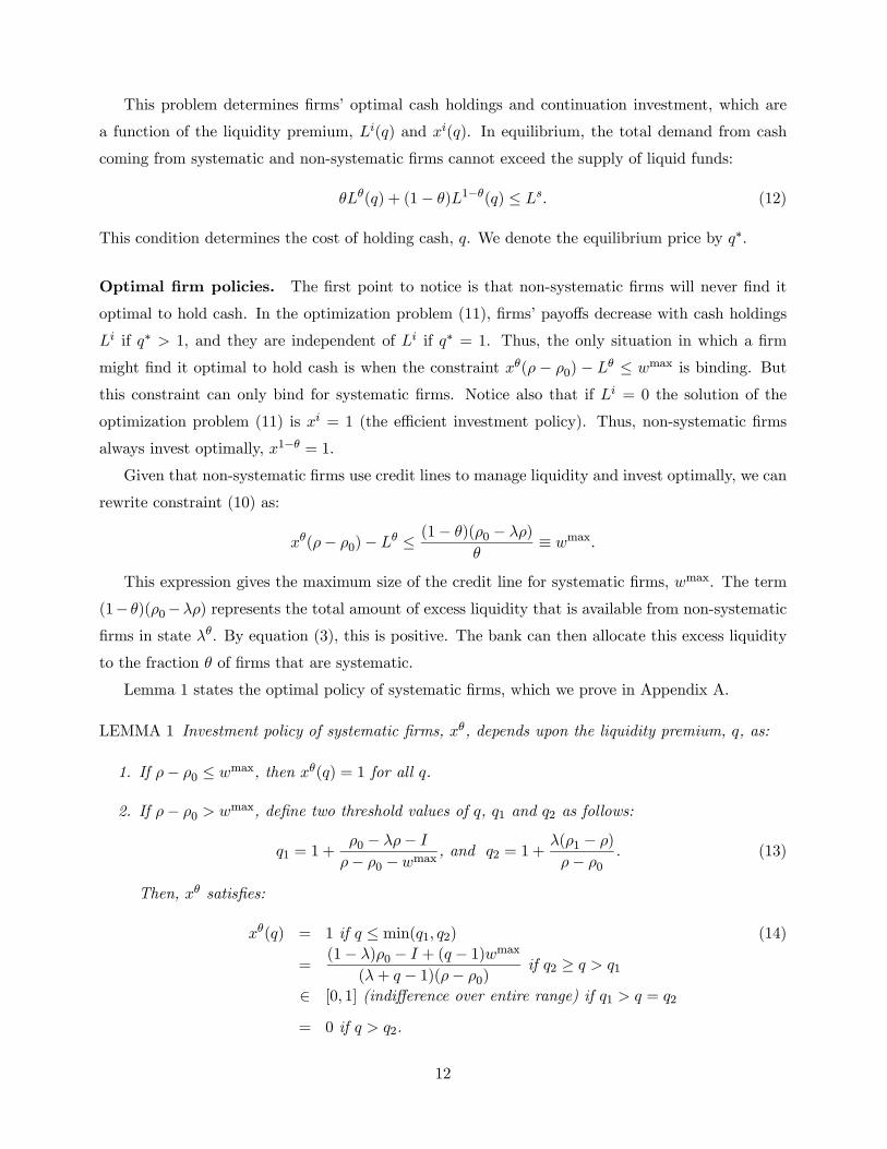
Lemma 1 states the optimal policy of systematic firms, which we prove in Appendix A.

LEMMA 1 Investment policy of systematic firms, xθ, depends upon the liquidity premium, q, as:

1. If ρ− ρ0 ≤ wmax, then xθ(q) = 1 for all q.

2. If ρ− ρ0 > wmax, define two threshold values of q, q1 and q2 as follows:

q1 = 1 +ρ0 − λρ− I

ρ− ρ0 −wmax, and q2 = 1 +

λ(ρ1 − ρ)

ρ− ρ0. (13)

Then, xθ satisfies:

xθ(q) = 1 if q ≤ min(q1, q2) (14)

=(1− λ)ρ0 − I + (q − 1)wmax

(λ+ q − 1)(ρ− ρ0)if q2 ≥ q > q1

∈ [0, 1] (indifference over entire range) if q1 > q = q2

= 0 if q > q2.

12

In words, systematic firms will invest efficiently if their total liquidity demand (ρ − ρ0) can be

satisfied by credit lines (of maximum size wmax), or if the cost of holding cash q is low enough. If

the maximum available credit line is low, and the cost of carrying cash is high, then systematic firms

will optimally reduce their optimal continuation investment (xθ < 1). If the cost of carrying cash is

high enough, then systematic firms may need to fully liquidate their projects (xθ = 0).

Given the optimal investment in Lemma 1, the demand for cash is given by Lθ(q) = 0 if ρ−ρ0 ≤wmax, and by the following condition

Lθ(xθ) = xθ(ρ− ρ0)− wmax, (15)

when ρ− ρ0 > wmax, for the optimal xθ(q) in Lemma 1.

Equilibria. The particular equilibrium that obtains in the model will depend on the fraction of

systematic firms in the economy (θ), and the supply of liquid funds (Ls).

First, notice that if ρ − ρ0 ≤ wmax (that is, if the fraction of systematic firms in the economyis small, (θ ≤ θmax), then there is no cash demand and the equilibrium liquidity premium is zero

(q∗ = 1). Firms use credit lines to manage liquidity and they invest efficiently (xθ = x1−θ = 1).

On the flip side, if ρ− ρ0 > wmax (that is, θ > θmax), then systematic firms will need to use cash

in equilibrium. Equilibrium requires that the demand for cash does not exceed supply:

θLθ(q) = θ[xθ(q)(ρ− ρ0)− wmax] ≤ Ls. (16)

Given this equilibrium condition, we can find the minimum level of liquidity supply Ls, such that

systematic firms can sustain an efficient investment policy, xθ(q) = 1. This is given by:

θ[(ρ− ρ0)− wmax] = Ls1(θ). (17)

If Ls ≥ Ls1(θ), then systematic firms invest efficiently, xθ = 1, demand a credit line equal to

wmax, and have cash holdings equal to Lθ = (ρ− ρ0)− wmax. The equilibrium liquidity premium is

zero, q∗ = 1. When Ls drops below Ls1(θ), then the cash demand by systematic firms must fall to

make it compatible with supply. This is accomplished by an increase in the liquidity premium that

reduces cash demand. In equilibrium, we have q∗ > 1, xθ(q∗) < 1, and equation (16) holding with

equality (such that the demand for cash equals the reduced supply):6

θ[xθ(q∗)(ρ− ρ0)−wmax] = Ls. (18)

6There are two cases to consider here, depending on whether q1 is higher or lower than q2. Please see the online

appendix for details.

13

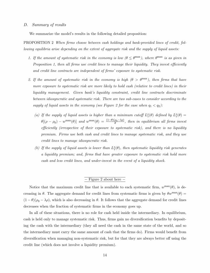
D. Summary of results

We summarize the model’s results in the following detailed proposition:

PROPOSITION 2 When firms choose between cash holdings and bank-provided lines of credit, fol-

lowing equilibria arise depending on the extent of aggregate risk and the supply of liquid assets:

1. If the amount of systematic risk in the economy is low (θ ≤ θmax), where θmax is as given in

Proposition 1, then all firms use credit lines to manage their liquidity. They invest efficiently

and credit line contracts are independent of firms’ exposure to systematic risk.

2. If the amount of systematic risk in the economy is high (θ > θmax), then firms that have

more exposure to systematic risk are more likely to hold cash (relative to credit lines) in their

liquidity management. Given bank’s liquidity constraint, credit line contracts discriminate

between idiosyncratic and systematic risk. There are two sub-cases to consider according to the

supply of liquid assets in the economy (see Figure 2 for the case when q1 < q2):

(a) If the supply of liquid assets is higher than a minimum cutoff Ls1(θ) defined by Ls1(θ) =

θ[(ρ − ρ0) − wmax(θ)] and wmax(θ) = (1−θ)(ρ0−λρ)θ

, then in equilibrium all firms invest

efficiently (irrespective of their exposure to systematic risk), and there is no liquidity

premium. Firms use both cash and credit lines to manage systematic risk, and they use

credit lines to manage idiosyncratic risk.

(b) If the supply of liquid assets is lower than Ls1(θ), then systematic liquidity risk generates

a liquidity premium; and, firms that have greater exposure to systematic risk hold more

cash and less credit lines, and under-invest in the event of a liquidity shock.

− Figure 2 about here −Notice that the maximum credit line that is available to each systematic firm, wmax(θ), is de-

creasing in θ. The aggregate demand for credit lines from systematic firms is given by θwmax(θ) =

(1− θ)(ρ0 − λρ), which is also decreasing in θ. It follows that the aggregate demand for credit lines

decreases when the fraction of systematic firms in the economy goes up.

In all of these situations, there is no role for cash held inside the intermediary. In equilibrium,

cash is held only to manage systematic risk. Thus, firms gain no diversification benefits by deposit-

ing the cash with the intermediary (they all need the cash in the same state of the world, and so

the intermediary must carry the same amount of cash that the firms do). Firms would benefit from

diversification when managing non-systematic risk, but for that they are always better off using the

credit line (which does not involve a liquidity premium).

14

E. Empirical implications

The model generates the following implications, which we examine in the next section:

(1) An increase in a firm’s exposure to systematic risk increases its propensity to use cash re-

serves for corporate liquidity management, relative to bank-provided lines of credit. We test this

prediction by relating the fraction of total corporate liquidity that is held in the form of credit lines

to proxies for a firm’s systematic risk exposure (e.g., beta).

(2) A firm’s exposure to risks that are systematic to the banking industry is particularly important

for the determination of its liquidity policy. In the model, bank systematic risk has a one-to-one

relation with firm systematic risk, given that there is only one source of risk in the economy (firms’

liquidity shock). However, one might imagine that in reality banks face other sources of system-

atic risk (coming, for example, from consumers’ liquidity demand) and that firms are differentially

exposed to such risks. Accordingly, a “firm-bank asset beta” should also drive corporate liquidity

policy. Firms that are more sensitive to banking industry downturns should be more likely to hold

cash for liquidity management.

(3) The trade-off between cash and credit lines is more important for firms that find it more

costly to raise external capital. In the absence of financing constraints, there is no role for corporate

liquidity policy, thus the choice between cash and credit lines becomes irrelevant. We test this model

implication by sorting firms according to observable proxies for financing constraints, and examining

whether the effect of systematic risk exposure on the choice between cash and credit lines is driven

by firms that are likely to be financially constrained.

(4) The effect of systematic risk exposure on corporate liquidity policy should be greater among

firms with high systematic risk. In the model, the effect of systematic risk on corporate liquidity

policy is non-linear (convex). If aggregate risk exposure is low (for example, if θ is low, then the

bank’s liquidity constraint does not bind, and thus variation in systematic risk exposure does not

matter. After θ reaches the threshold level θmax, further increases in aggregate risk exposure tighten

the bank’s liquidity constraint and thus forces firms to switch to cash holdings. We test this im-

plication by examining whether the effect of aggregate risk exposure (beta) on liquidity policy is

concentrated among firms with high systematic risk exposure (e.g., beta).7

(5) Firms with higher systematic risk exposure should face worse contractual terms when raising

bank credit lines. In the model, if the amount of systematic risk in the economy is high, then the

7Strictly speaking, in the model the variable θ captures the amount of systematic risk in the economy as a whole.

In addition, the model only allows for two types of firms (systematic and idiosyncratic). However, a similar implication

would hold in a version of the model in which firms varied continuously with respect to their aggregate risk exposure.

Low beta firms create little liquidity risk for the bank, and thus there would be a cutoff below which all firms would

have access to cheap credit lines. Only high beta firms would be driven out of bank credit lines, and more so the

greater the value of beta.

15

bank’s liquidity constraint requires that credit line contracts discriminate between idiosyncratic and

systematic risk. Systematic firms should face worse contractual terms since they are the ones that

drive the bank’s liquidity constraint. We test this implication by relating asset beta to credit line

spreads and fees, after controlling for firm characteristics and other credit line contractual terms.

(6) An increase in the amount of systematic risk in the economy increases firms’ reliance on cash

and reduces their reliance on credit lines for liquidity management. The model shows that when

economy-wide aggregate risk is low, firms can manage their liquidity using only credit lines because

the banking sector can provide them at actuarially fair terms. When aggregate risk increases beyond

a certain level, firms must shift away from credit lines and towards cash so that the banking sector’s

liquidity constraint is satisfied.8 In addition, the greater is the amount of systematic risk in the

economy, the lower is the amount of liquidity that is provided by bank credit lines. We test this

implication by examining how aggregate cash holdings and credit line initiations change with VIX,

the implied volatility of the stock market index returns from options data. In addition, and similarly

to Implication 2 above, we also examine whether “Bank VIX ”, a measure we compute of the expected

volatility in the banking sector, drives time-series variation in corporate liquidity policy.

(7) An increase in the amount of systematic risk in the economy worsens firms’ contractual

terms when raising bank credit lines. We test this implication by examining how credit line spreads

and maturities change with changes in economy-wide risk (VIX ) and banking sector (Bank VIX )

aggregate risk.9

II. Empirical tests

A. Data

We use two alternative sources to construct our line of credit data. Our first sample (which

we call LPC Sample) is drawn from LPC-DealScan. These data allow us to construct a large sam-

ple of credit line initiations. We note, however, that the LPC-DealScan data have two potential

drawbacks. First, they are mostly based on syndicated loans, thus are potentially biased towards

large deals and consequently towards large firms. Second, they do not allow us to measure line of

credit drawdowns (the fraction of existing lines that has been used in the past). To overcome these

issues, we also construct an alternative sample that contains detailed information on the credit lines

initiated and used by a random sample of 300 COMPUSTAT firms. These data are provided by

8In section C.3., we provide evidence that exposure to undrawn corporate credit lines increases bank stock return

volatility in times of high aggregate risk. This result is consistent with the mechanism suggested by the model, whereby

credit line exposure poses risks to banks when corporate liquidity shocks become correlated.9Our model has the additional empirical implication that the liquidity risk premium is higher when there is an

economic downturn since in such times there is greater aggregate risk and lines of credit become more expensive. This

is similar to the result of Eisfeldt and Rampini (2009), but in their model, the effect arises from the fact that firms’

cash flows are lower in economic downturns and they are less naturally hedged against future liquidity needs.

16

Amir Sufi on his website and were used on Sufi (2009). We call this sample Random Sample. Using

these data reduces the sample size for our tests. In particular, since this sample only contains seven

years (1996-2003), in our time-series tests we use only LPC sample. We regard these two samples

as providing complementary information on the usage of credit lines for the purposes of this paper.

The data construction criteria are described in detail in Appendix B.

B. Variable definitions

Our main variables of interest are described below. All of our control variables in tests are as in

Sufi (2009). Detailed description of the variables is in Appendices C, D and E.

Line of credit data. When using Random Sample, we measure the fraction of total corporate

liquidity that is provided by credit lines for firm i in year t using the ratios of both total and unused

credit lines to the sum of credit lines plus cash. As discussed by Sufi, while some firms may have

higher demand for total liquidity due to better investment opportunities, these LC-to-Cash ratios

should isolate the relative usage of lines of credit versus cash in corporate liquidity management.

When using LPC Sample, we construct a proxy for line of credit usage in the following way.

For each firm-quarter, we measure credit line availability at date t by summing all existing credit

lines that have not yet matured (Total LC). We convert these firm-quarter measures into firm-year

measures by computing the average value of Total LC in each year. We then measure the fraction

of corporate liquidity that is provided by lines of credit by computing the ratio of Total LC to the

sum of Total LC plus cash.

In addition, to examine the time-series impact of systematic risk on liquidity management we

construct aggregate changes in credit lines and cash, scaled by assets (LC Initiationt and Change

in Casht). These ratios capture the economy’s total demand for cash and credit lines in a given

year, scaled by total assets.

Data on betas and variances. We measure firms’ exposure to systematic risk using asset (unlev-

ered) betas.10 While equity betas are easy to compute using stock price data, they are mechanically

related to leverage: high leverage firms will tend to have larger betas. Because greater reliance on

credit lines will typically increase the firm’s leverage, the leverage effect would then bias our esti-

mates of the effect of betas on corporate liquidity management. Nonetheless, we also present results

using standard equity betas (Beta Equity).

We unlever equity betas in two alternative ways. First, we use a Merton-KMV type model to

unlever Betas (Beta KMV ), and total asset volatility (Var KMV ). Second, we use Choi (2009) betas

10Similar to the COMPUSTAT data items, all measures of beta described below are winsorized at a 5% level.

17

and asset variance (denoted Beta Asset and Var Asset). Because of data availability, we use Beta

KMV as our benchmark measure of beta, but we verify that the results are robust to the use of this

alternative unlevering method.

One potential concern with theses beta measures is that they may be mechanically influenced

by a firm’s cash holdings. Since corporate cash holdings are typically held in the form of riskless

securities, high cash firms could have lower asset betas. Thus, we also compute KMV-type asset

betas that are unlevered using net debt (e.g., debt minus cash) rather than gross debt. We call this

variable Beta Cash, which is computed at the level of the industry to mitigate endogeneity. We also

compute a firm’s “bank beta” (which we call Beta Bank) to test the model’s implication that a firm’s

exposure to banking sector’s risks should influence the firm’s liquidity policy. In the model, a firm’s

exposure to systematic risks matters mostly on the downside (because a firm may need liquidity

when other firms are likely to be in trouble). To capture a firm’s exposure to large negative shocks,

we follow Acharya, Pedersen, Philippon, and Richardson (2010) and compute the firm’s Beta Tail.

All of the betas described above are computed using market prices. As discussed in the intro-

duction, using market data is desirable because of their high frequency, and because they also reflect

a firm’s financing capacity that is tied to its long-run prospects. However, the model’s argument

is based on the correlation between a firm’s liquidity needs, and the liquidity need for the overall

economy (which affects the banking sector’s ability to provide liquidity). While market-based betas

should capture this correlation, it is desirable to verify whether a beta that is based more directly on

cash flows and financing needs also contains information about firm’s choices between cash and credit

lines. In order to do this, we compute two alternative beta proxies (Beta Gap and Beta Cash Flow).

Decomposing total risk into idiosyncratic and systematic components. In addition to

using asset and cash flow betas to measure systematic risk exposure, we alternatively use a measure of

systematic risk which is computed by decomposing total asset risk on its systematic and idiosyncratic

components. Using the Merton-KMV betas and variances, the systematic component for firm j at

time t can be estimated as:

SysV ar KMVj,t = (Beta KMVj,t)2 × V ar KMVt, (19)

where V ar KMVt is the unlevered variance of the market. We compute V ar KMVt as the value-

weighted average of firm-level asset variances, Var KMV j,t. The systematic component is essentially

the variance of asset returns that is explained by the market. Given this formula, the idiosyncratic

component can be computed as total asset variance V ar KMVj,t minus SysV ar KMVj,t.

Notice that since idiosyncratic variance is a function of total and systematic variance, we do

not need to include it separately in the corporate liquidity regressions. Rather, we experiment with

18

specifications in which we include both total and systematic variance (or beta) in the regressions

explaining corporate liquidity.

Addressing measurement error. A common shortcoming of the measures of systematic risk we

constructed is that they are noisy and subject to measurement error. This problem can be ame-

liorated by adopting a strategy dealing with classical errors-in-variables. We follow the standard

Griliches and Hausman (1986) approach to measurement problem and instrument the endogenous

variable (e.g., our beta proxies) with lags of itself. We experimented with alternative lag struc-

tures and chose a parsimonious form that satisfies the restriction conditions needed to validate the

approach.11 Throughout the analysis, we report auxiliary statistics that speak to the relevance

(first-stage F -tests) and validity (Hansen’s J -stats) of our instrumental variables regressions.

Time-series variables. We proxy for the extent of aggregate risk in the economy by using V IX

(the implied volatility on S&P 500 index options). VIX captures both aggregate volatility, as well

as the financial sector’s appetite to bear that risk. We also add other macroeconomic variables to

our tests, including the commercial paper—Treasury spread (Gatev and Strahan (2005)) to capture

the possibility that funds may flow to the banking sector in times of high aggregate volatility, and

real GDP growth to capture general economic conditions.

In addition, we proxy for the extent of aggregate risk in the banking sector by computing Bank

V IX (the expected volatility on an index of bank stock returns). Since there are no available his-

torical data on implied volatility for an aggregate bank equity index, we compute expected volatility

using a GARCH (1,1) model and the Fama-French index of bank stock returns. The online appendix

details the procedure that we use.

C. Empirical tests and results

Summary statistics. We start by summarizing our data in Table 1. Panel A reports summary

statistics for the LPC-DealScan sample (for firm-years in which Beta KMV data are available), and

Panel B uses Sufi’s sample. Notice that the size of the sample in Panel A is much larger, and that

the data for Beta Asset are available only for approximately one third of the firm-years for which

Beta KMV data are available. As expected, the average values of asset betas are very close to each

other, with average values close to one. The two alternative measures of variance also appear to

be very close to each other. The spread and fee data are available at the deal-level, and thus the

number of observations reflect the number of different credit line deals in our sample.

− Table 1 about here −11An alternative way to address measurement error is to compute betas at a “portfolio,” rather than at a firm-level.

We explore this idea as well, using industry betas rather than firm-level betas in some specifications below.

19

Comparing Panel A and Panel B, notice that the distribution for most of the variables is very sim-

ilar across the two samples. The main difference between the two samples is that the LPC-DealScan

data is biased towards large firms (as discussed above). For example, median assets are equal to

270 million in LPC Sample, and 116 million in Random Sample. Consistent with this difference,

the firms in LPC Sample are also older, and have higher average Qs and EBITDA volatility. The

measure of line of credit availability in LPC Sample (LC-to-Cash) is lower than those in Random

Sample (Total LC-to-Cash and Unused LC-to-Cash). For example, the average value of LC-to-Cash

in LPC Sample is 0.33, while the average value of Total LC-to-Cash is 0.51. This difference reflects

the fact that LPC-DealScan may fail to report some credit lines that are available in Sufi’s data,

though it could also reflect the different sample compositions.

In Table 2, we examine the correlation among the different betas that we use in this study. We

also include the asset variance proxies (Var KMV, Var Asset, and SysVar KMV ). Not surprisingly,

all the beta proxies that are based on asset return data are highly correlated. The lowest correlations

are those between the cash flow-based betas (Beta Gap and Beta Cash Flow) and the asset-return

based betas (approximately 0.10). The correlations among the other betas (all of them based on

asset return data) hover between 0.3 and 0.9.

− Table 2 about here −

To examine the effect of aggregate risk on the choice between cash and credit lines, we perform

a number of different sets of tests. We describe these tests in turn.

C.1. Firm-level regressions

Our benchmark empirical specification closely follows of Sufi (2009). We expand his specification

by including our measure of systematic risk:

LC-to-Cashi,t = α+ β1BetaKMV i,t + β2 ln(Age)i,t + β3(Profitability)i,t−1 (20)

+β4Sizei,t−1 + β5Qi,t−1 + β6Networthi,t−1 + β7IndSalesV olj,t

+β8ProfitV oli,t +Xt

Y eart + ²i,t,

where Year absorbs time-specific effects, respectively. Our theory predicts that the coefficient β1

should be negative. We also run the same regression replacing Beta KMV with our other proxies

for a firm’s exposure to systematic and idiosyncratic risks (see Section B.). And we use different

proxies for LC-to-Cash, which are based both on LPC-DealScan and Sufi’s data. We also include

industry dummies (following Sufi we use 1-digit SIC industry dummies) and the variance measures

that are based on stock and asset returns (Var KMV and Var Asset).

20

The results for the KMV-Merton betas and variances, and LPC-DealScan data are presented in

Table 3. In column (1), we replicate Sufi’s (2009) results (see his Table 3). Just like Sufi, we find

that profitable, large, low Q, low net worth, low cash flow volatility firms are more likely to use bank

credit lines. The fact that we can replicate Sufi’s results is important, given that our dependent

variable is not as precisely measured as that in Sufi. In column (2), we introduce asset variance (Var

KMV ) in the model. Var KMV is negatively correlated with the LC-to-Cash ratio, and it drives out

the significance of Sufi’s profit volatility variable. This finding suggests that Var KMV is a better

measure of total risk than the profit volatility variable used by Sufi.


Next, we introduce our measures of systematic risk in the regressions. The coefficient on Beta

KMV in column (3) suggests that systematic risk is negatively related to the LC-to-Cash ratio. The

size of the coefficient implies that a one-standard deviation increase in asset beta (approximately 1)

decreases firm’s reliance on credit lines by approximately 0.08 (about 20% of the standard deviation

of the LC-to-Cash variable). In column (4) we use SysVar KMV in the regressions rather than Beta

KMV. The results again suggest that systematic risk exposure is negative correlated to the LC-to-

Cash ratio. Finally, in column (5) we report a specification that includes both Beta KMV and Var

KMV together in the same regressions. The coefficient on Beta KMV drops to approximately 0.06

and continues to be statistically significant (p-value equal to 1.78). The coefficient on Var KMV

remains negative but is not statistically significant.

Table 4 uses Sufi’s (2009) measures of LC-to-Cash rather than LPC-DealScan data. In columns

(1) to (4) we use Total LC-to-Cash, and in columns (5) to (8) we use Unused LC-to-Cash. Columns

(1) and (5) replicate the results in Sufi’s Table 3. Notice that the coefficients are virtually identical

to those in Sufi. We then introduce our KMV-based proxies for total, and aggregate risk exposures.

As in Table 3, the evidence suggests that systematic risk exposure is negatively correlated with the

use of credit lines. We reach this conclusion both when we use Beta KMV (columns (2) and (6)) and

SysVar KMV (columns (3) and (7)) to proxy for systematic risk exposure. In addition, aggregate

risk exposure continues to be significantly related to the LC-to-Cash ratio after controlling for Var

KMV (columns (4) and (8)). These results suggest that the cross-sectional relationship between sys-

tematic risk exposure and liquidity management is economically significant and robust to different

ways of computing exposure to systematic risk and reliance on credit lines.12

− Table 4 about here −12 In our model, both cash and credit lines are used by the firm to hedge liquidity shocks. This raises the question

of whether derivatives-based hedging would affect our results. We believe this is unlikely for a couple of reasons.

First, notice that the use of derivatives and other forms of hedging should be reflected in the betas that we observe.

Second, while derivatives hedging is only feasible in certain industries (such as those that are commodity-intensive),

our results hold across and within industries, for a broad set of industries.

21

It is important that we consider the validity of our instrumental variables approach to the mis-

measurement problem. The first statistic we consider in this examination is the first-stage exclusion

F -tests for our set of instruments. Their associated p-values are all lower to 1% (confirming the

explanatory power of our instruments). We also examine the validity of the exclusion restrictions

associated with our set of instruments. We do this using Hansen’s (1982) J -test statistic for overiden-

tifying restrictions. The p-values associated with Hansen’s test statistic are reported in the last row

of Tables 3 and 4. We generally find high p-values (particularly when using Sufi’s sample in Table 4).

These reported statistics suggest that we do not reject the joint null hypothesis that our instruments

are uncorrelated with the error term in the leverage regression and the model is well-specified.

Table 5 replaces Beta KMV with our alternative beta measures using the LPC-Deal Scan sam-

ple.13 The results in the first column of Table 5 suggest that the results reported in Table 3 are robust

to the method used to unlever betas. Beta Asset (which is based directly on asset return data) has

a similar relation to liquidity policy as that uncovered in Table 2. The economic magnitude of the

coefficient on Beta Asset is in fact larger than that reported in Table 2. Using industry-level cash-

adjusted betas, Beta Cash, also produces similar results (column (2)). In column (3), we show that a

firm’s exposure to banking sector risks (Beta Bank) affects liquidity policy in a way that is consistent

with the theory. The coefficients are also economically significant. Specifically, a one-standard devi-

ation increase in Beta Bank (which is equal to 0.7) decreases LC-to-Cash by 0.21, which is half of the

standard deviation of the LC-to-Cash variable. Column (4) shows that a firm’s exposure to tail risks

is also correlated with liquidity policy. Firms which tend to do poorly during market downturns have

a significantly lower LC-to-Cash ratio. In column (5), we use equity (levered) betas instead of asset

betas. The coefficient on beta is comparable to the similar specification in Table 3 (which is in column

(3)), though somewhat smaller. Thus, adjusting for the leverage effect increases the effect of beta

on the LC-to-Cash ratio (as expected). However, even the equity beta shows a negative relation to

the fraction of credit lines used in liquidity management. Columns (6) and (7) replace market-based

beta measures with cash flow-based betas computed at the industry level (Beta Gap and Beta Cash

Flow). Consistent with the theory, cash flow betas are significantly related to the LC-to-Cash ratio,

though economic significance is smaller than for the market measures.14 Finally, in column (8) we

use value-weighted industry betas rather than firm-level betas in the regression. Using industry betas

is an alternative way to address the possibility that firm-level betas are measured with error. Thus,

in column (6) we do not instrument betas with the first two lags (as we do in the other columns).

13We obtain similar results when using Sufi’s sample (see the internet appendix).14The coefficient in column (7), for example, suggests that a one-standard deviation increase in Beta Gap decreases

LC-to-Cash by approximately 1.5%.

22

The results again suggest a significant relation between asset beta and the LC-to-Cash ratio.


The regressions on Tables 3 and 4 suggest that total risk is not robustly related to corporate

liquidity policy, after introducing proxies for systematic risk exposure (such as Beta KMV ). In other

words, firms’ idiosyncratic or non-systematic risk is not robustly related to cross-sectional variation

in liquidity policy. This result may appear to contradict the results in Sufi (2009), who suggests that

riskier firms should shy away from credit lines due to the risk of covenant violations. However, Sufi

(2009) also shows that the level of profitability proxies for the risk of covenant violations and credit

line revocations. In particular, the level of profitability is the key variable that predicts covenant

violations (as shown in Sufi’s Table 6). The results above are consistent with Sufi’s profitability

results, since the level of profitability in our results too is positively related to the LC-Cash ratio,

particularly so in the LPC sample (Tables 3 and 5), suggesting that the risk of credit line revocation

is being captured by variation in the level of profitability, rather than non-systematic risk.

Sorting firms according to proxies for financing constraints and beta. One of the implica-

tions of the model in Section I. is that the choice between cash and credit lines should be most relevant

for firms that are financially constrained (Implication 3). This line of argument suggests that the

relation that we find above should be driven by firms that find it more costly to raise external funds.

In addition, the theory suggests that the effect of systematic risk exposure on corporate liquidity

policy should primarily arise among firms with high systematic risk (Implication 4). In this section

we attempt to test both implications. We follow prior studies (e.g., Almeida, Campello and Weisbach

(2004)) in using three alternative schemes to partition our sample in order to test Implication 3:

(1) We rank firms based on their payout ratio and assign to the financially constrained (uncon-

strained) group those firms in the bottom (top) three deciles of the annual payout distribution.

(2) We rank firms based on their asset size, and assign to the financially constrained (uncon-

strained) group those firms in the bottom (top) three deciles of the size distribution. The argument

for size as a good observable measure of financial constraints is that small firms are typically young,

less well known, and thus more vulnerable to credit imperfections.

(3) We rank firms based on whether they have bond and commercial paper ratings. A firm is

deemed to be constrained if it has neither a bond nor a commercial paper rating. it is unconstrained

if it has both a bond and a commercial paper rating.

To test Implication 4, we partition the sample into two groups. “High Beta” firms are those that

have beta greater than one. “Low Beta” firms are those that have beta less than one (the average

value of Beta KMV according to Table 1).

23

We repeat the regressions performed above, but now separately for financially constrained and

unconstrained subsamples and for Low Beta and High Beta sub-samples. To measure systematic

risk, we use both Beta KMV and Beta Tail (which measures firms’ exposure to tail risks).

Table 6 presents the results we obtain. Panel A presents results for Beta KMV, and Panel B

shows the Beta Tail results. Results for the other beta proxies are generally similar, and are pre-

sented in the internet appendix. The first six columns in Panel A show that the negative relation

between systematic risk and the usage of credit lines obtains only in the constrained samples. The

coefficient on Beta KMV for the constrained samples is negative and significant for the small and

low payout samples, but is insignificant for large, high payout, and rated firms. Column (5) shows

that the coefficient is negative but not significant for non-rated firms (t-stat of 1.47). The coeffi-

cients are also significantly different across constrained and unconstrained samples, with exception

of the ratings sorting. The p-values from Wald tests that the coefficients are significantly different

from each other range from 0.198 (ratings sorting) to 0.005 (payout sorting). Panel B shows similar

results for the Beta Tail variable. The main differences are that the coefficient on Beta Tail for

the non-rated sub-sample is now significantly negative (t-stat of −4.56), while the coefficient for thehigh-payout sample is now negative and significant. However, even for the payout sorting there is

(weak) evidence that the coefficient is larger for the constrained sample. The p-value from a Wald

test that the coefficient for the low payout sample is different from that for the high payout sample

is 0.104. The p-values are higher for the ratings (p-value of 0.037) and the size sortings (p-value of

0.003), indicating that the coefficient on Beta for constrained samples is indeed more negative than

that for unconstrained samples. These results are consistent with Implication 3.


Columns (7) and (8) of each Panel show that the negative relationship between beta and the

LC-Cash ratio is much stronger in the sample of firms with high exposure to aggregate risk. When

using Beta KMV, the negative coefficient on beta obtains only in the High Beta sample. The coef-

ficient is negative and significant for the Low Beta sample when using Beta Tail, but its magnitude

is substantially smaller than the coefficient that obtains in the High Beta sample. The p-value from

a Wald test that the coefficients on Beta Tail are different from each other is 0.024, indicating that

the coefficients are statiscally distinguishable from each other. These results support Implication 4.

The non-linearity of the relationship between beta and the LC-Cash ratio can also be illustrated

with a graph. In Figure 3, we sort the sample into quintiles based on the average value for Beta

KMV for each firm during the entire sample period. Then, we calculate the average value of the

LC-Cash ratio in each of these quintiles of beta. Figure 3 shows that the average LC-Cash ratio

barely changes as one moves from the first to the third quintile of Beta (the average LC-Cash ratio

24

in the first three quintiles is approximately 0.35). However, the average ratio in the highest quintile

drops to less than 0.2. This figure gives a visual illustration that the effect of beta on the LC-Cash

ratio is concentrated among firms with high exposure to systematic risk (Implication 4 of the theory).


Asset beta and the cost of credit lines. The empirical findings so far all suggest that firms

with high aggregate risk exposure hold more cash relative to lines of credit. This effect arises in our

theoretical model since firms with greater aggregate risk exposure face a higher cost of bank lines

of credit. We perform an additional test to further investigate this channel. Specifically, we provide

evidence on the relation between all-in drawn spreads and undrawn fees paid by firms on their credit

lines, and systematic risk. To do this, we regress the average annual spreads and fees paid by firm

i in deals initiated in year t,15 on systematic risk proxies and controls. We control for the size of

credit line facilities raised in year t scaled by assets (LCi,t

Assetsi,t), and the level of the LIBOR in the

quarter when the credit line was raised.16 Our empirical model has the following form:

Costi,t=μ0 + μ1Betai,t + μ2(LCi,t

Assetsi,t) + μ3LIBORi,t +μ4Xi,t +

Xt

Y eart + ²i,t, (21)

where X is the vector of firm characteristics used in equation (20). We use both All-in drawn spread

and Undrawn fee as alternative dependent variables to measure the cost of credit lines. We focus on

a set of three risk proxies (namely, Beta KMV, Beta Tail, and SysVar KMV ), and present results

for the other proxies in the internet appendix.

Our findings are presented in Table 7. The coefficients on systematic risk proxies in columns

(1) to (3) suggest that All-in drawn spread is higher for firms with greater exposure to systematic

risk (though statistical significance for the coefficient on Beta KMV is weaker).17 For example,

the coefficient estimate of 10 on SysVar KMV indicates that a one-standard deviation change in

systematic risk exposure (equal to 0.018 according to Table 1) is associated with an increase of 18

basis points on credit line spreads (approximately 16% of the standard deviation in All-in drawn

spread). Columns (4) through (6) show similar results for Undrawn fee. The evidence suggests that

an increase of one standard deviation in systematic risk exposure increases undrawn fees by 6 basis

points, 35% of the standard deviation reported in Table 1. These results provide evidence that firms

with high exposure to systematic risk face worse contractual terms when initiating credit lines.

− Table 7 about here −15This annual average is weighted by the amount raised in each credit line deal.16The data on LIBOR refers to the level of LIBOR in the quarter in which firm i initiates the credit line. We

annualize this variable by computing the facility size-weighted, firm-year average (LIBORi,t). Notice that since firms

initiate credit lines in different quarters, this proxy varies both over time and across firms.17We obtain generally similar results for the other systematic risk proxies (see the internet appendix).

25

C.2. Time-series tests

In this section, we examine the time-series implications of the model. The model suggests that an

increase in aggregate risk makes it more difficult for the banking sector to provide new credit lines.

Accordingly, high aggregate risk should be associated with lower credit line initiations, and worse

terms for new credit lines (for example, higher spreads and shorter maturities). In response, firms

should attempt to build up cash reserves. The model also suggests that both economy-wide and

banking sector risk should matter for corporate liquidity policy. We examine these dynamics in turn.

We focus first on the impact of aggregate risk on credit line initiations and changes in cash hold-

ings (defined in equation (38) in the appendix). To do so, we run the following time-series SURmodel:

LCInitiationt = ς0 + ς1V IXt−1 + ς2TimeTrendt + ς3Controlst−1 +$t (22)

Change in Casht = γ0 + γ1V IXt−1 + γ2Time Trendt + γ3Controlst−1 + υt.

To allow for variation in our tests, in some specifications we replace V IX (a measure of economy-wide

aggregate risk) with Bank V IX (expected volatility of banking sector equity returns).18 We also

include both volatility measures together in the regressions in some specifications. Our model would

suggest that ς1 < 0, and γ1 > 0. The control variables are the 3-month commercial paper—Treasury

spread and real GDP growth. Previous banking literature suggests that during crises, banks expe-

rience an inflow of deposits coming from the commercial paper market. This effect, in turn, helps

them honor their loan commitments (e.g., Gatev and Strahan (2005)). Banks’ increased ability to

honor their commitments during bad times may then counteract the effect of V IX on corporate

liquidity management. As shown by Gatev and Strahan, this inflow effect tends to happen in times

when the spread of commercial paper over Treasury rates is high. Real GDP growth captures general

economic conditions and investment opportunities. We lag both V IX and the control variables one

period, since it may take time for macroeconomic conditions to affect corporate liquidity manage-

ment variables. Also, corporate variable may be measured at different times of the year based on

fiscal-year ends.

Before reporting the results, we examine the relation between V IX, LC Initiation, and Change

in Cash in a simple plot. Figure 4 shows a clear negative correlation between VIX and credit line

initiations in our sample period. The correlation between V IX and changes in cash is less clear, but

there seems to be a positive correlation throughout the sample period.


Table 8 reports the regression outputs. The results for credit lines are presented in Panel A,

and those for cash are in Panel B (recall that each equation is estimated using a SUR procedure).

18The correlation between V IX and Bank V IX in our time-series data is equal to 0.39.

26

Column (1) shows that the negative relation between V IX and LC Initiation is statistically sig-

nificant. The coefficient on V IX suggests that a one-standard deviation increase in V IX (which is

equal to 0.07) decreases LC Initiation by approximately 0.7 standard deviations of that variable.

This effect is economically relevant. In addition, V IX has a positive relation with aggregate change

in cash holdings. The coefficient on Panel B suggests that a one-standard deviation in V IX in-

creases aggregate cash holdings by 0.43 standard deviations of that variable. Column (2) suggests

that Bank V IX also has a negative relation with LC Initiation. However, the coefficient on the

cash regression is virtually zero. When we include both V IX and Bank V IX together in the same

regression (see column (3)), we find that both are negatively related to LC Initiation, suggesting

that banking sector matters for credit line provision, over and above economy-wide aggregate risk.

This result supports the implications of our model.


One potential issue with the results above is that the right-hand side variables are simple aggre-

gates (see equation (38)). In particular, these results leave open the possibility that contemporaneous

changes in other firm-level variables may affect our inferences. In order to address this possibility,

in columns (4) to (6) we use the average residual value of firm-level cash holdings and credit line

initiations to compute our aggregate quantities. The firm-level residual values are computed using

the same explanatory variables as in equation (20) (excluding year effects and Beta). Columns (4)

through (6) show that our results become even stronger after this change in the specification. While

the relation between V IX, LC Initiation, and Change in Cash is robust to this modification (col-

umn (4)), column (5) shows that Bank V IX is now positively correlated with Change in Cash. In

addition, column (6) suggests that both V IX and Bank V IX seem to matter for corporate liquidity

policy in the way suggested by our theory.19

Table 8 suggests that in times of high aggregate risk, new credit line initiations decrease and

cash holdings increase. Thus, firms appear to be substituting cash holdings for credit lines when

aggregate risk is high. This pattern is consistent with our model, which predicts that the banking

sector’s ability to provide new credit lines decreases when aggregate risk is high. However, there are

other explanations for the correlations depicted in Table 8. For example, even though we control

for GDP growth, it is possible that V IX is capturing general economic conditions, which reduce

investment opportunities and firms’ demand for new credit lines. Second, it is possible that aggre-

gate risk increases the cost of debt for corporations, causing firms to reduce demand for any type of

19We also performed tests of joint significance for V IX and Bank V IX in the regressions depicted in columns (3)

and (6), both for credit line initiations and cash (Panels A and B). In all cases we reject the hypothesis that the

coefficients on V IX and Bank V IX are jointly equal to zero (the highest p-value that we obtain is approximately

0.03, in the cash regression in column (3)).

27

debt (including credit lines).20 It is thus important that we perform tests that are designed to help

counter these alternative explanations and provide additional support for our model.

To address the possibility that the results in Table 8 capture a decrease in overall demand for

credit and liquidity in the economy, we examine aggregate changes in credit line contractual terms

(spreads and maturities). The idea is as follows. If the reduction in credit line initiations reflects

a decline in demand that is caused by poor investment opportunities, then we would expect the

spreads on new credit lines to decrease as well (as the economy moves along the supply curve, and

adjusts to the reduction in credit line demand). On the other hand, if the underlying cause for the

decline in observed initiations is as suggested by our model, then we would expect credit line spreads

to increase following an increase in VIX. In addition, according to our model, we would also expect

other contractual terms such as credit line maturities to become tighter (e.g., shorter maturities).

We examine the relation between V IX, Bank V IX, and credit line terms in the four first

columns of Table 9. To do so, we measure the average credit line maturity and all-in drawn spread

(weighted by the size of the credit line facility) in each year of our sample. We then estimate a SUR

model in which average maturities and spreads are used as dependent variables:

Average Maturityt = ψ0 + ψ1V IXt−1 + ψ2TimeTrendt + ψ3Controlst−1 + κt (23)

Average Spreadt = %0 + %1V IXt−1 + %2TimeTrendt + %3Controlst−1 + φt.

The demand-investment opportunity story would suggest that ψ1 > 0 and %1 < 0, while our model

would predict ψ1 < 0 and %1 > 0.

The main result is presented in Table 9 and Figure 5. Notably, aggregate risk appears to tighten

credit line contractual terms. In other words, following increases in aggregate volatility, credit line

spreads increase, and maturities decrease. This result is visually obvious in Figure 5, and it is

confirmed in Table 9 (first four columns). In addition, notice that the impact of aggregate risk on

credit line contracts is economically substantial. A one-standard deviation increase in V IX decreases

average credit line maturity by approximately 60% of its standard deviation, and increases average

spread by 50% of its standard deviation.21 The results are similar for Bank V IX, though the

coefficient on the spread regression is not statistically significant.


− Table 9 about here −20For example, one argument is that financial distress costs are systematic and increase in times of high aggregate

risk (see Almeida and Philippon (2007) and Chen (2010)).21For example, the standard deviation in V IX is 0.07. Multiplying by the coefficient of −26 on the maturity

regression gives 1.82, which is 61% of the standard deviation of the maturity variable (which is equal to 3).

28

While these results are consistent with our model, they can still be explained by an overall in-

crease in the cost of debt for corporations, following an increase in aggregate risk. A simple way

to examine whether this is a plausible explanation for the results is to replace credit line initiations

with aggregate changes in total debt, and see whether lagged changes in aggregate risk also predict

reductions in total debt in the economy. We test this idea by estimating a debt-taking model in

which the dependent variable is computed similarly to changes in cash holdings:

Change in Debtt =

Pj(Debtj,t −Debtj,t−1)P

j Assetsj,t. (24)

In this equation, we define debt as the sum of short- and long-term debt from COMPUSTAT. We

then replace LCInitiationt in Equation 22 above with Change in Debtt.

Columns (5) and (6) of Table 9 report the results for the debt regression, using both V IX (col-

umn (5)) and Bank V IX (column (6)). The SUR model also includes an equation for Change in

Cash, but coefficients are not reported since they are identical to those reported in Table 9 (columns

(1) and (2)). As it turns out, neither lagged V IX nor Bank V ix predict an overall reduction in

debt in the economy. The coefficient on the Change in Debt variable is positive, economically small,

and statistically insignificant in column (5), and negative and statistically insignificant in column

(6). These results suggest that the negative impact of aggregate risk on new debt is strongest for

credit line initiations. This is consistent with our model’s suggestion that increases in aggregate risk

compromise the baking sector’s ability to provide credit lines for liquidity management.

C.3. Covenant violation risk or banks’ liquidity constraints?

The results above suggest that firms hold more cash and less credit lines when their aggregate risk

exposure is high, and when economy-wide aggregate risk increases. Our interpretation of these find-

ings is that aggregate risk increases the correlation among firms’ liquidity shocks, and tightens banks’

liquidity constraints, constraining banks’ ability to provide liquidity insurance to firms through credit

lines. Nevertheless, a possible alternative interpretation for the results is related to the risk of

covenant violations (as in Sufi (2009)). If firms are more likely to violate covenants in times when

aggregate risk is high, then “high beta” firms may shy away from credit lines not because of banks’ liq-

uidity constraint as in our model, but because of the risk of covenant violations. In this section, we at-

tempt to provide additional evidence that the link between liquidity management and aggregate risk

that our results uncovered is indeed due to the effect of aggregate risk on banks’ liquidity constraints.

Bank-level evidence on the link between credit line exposure and aggregate risk. First,

we devise a direct test of the prediction that aggregate risk exposure tightens banks’ liquidity con-

straints through a credit line channel. The link between credit line exposure and bank risk has

29

been studied by Gatev, Schuermann, and Strahan (2009). They find that bank risk, as measured

by stock return volatility, increases with unused credit lines that the bank has agreed to extend to

the corporate sector. The mechanism in our model would then suggest that the impact of credit

line exposure on bank risk should increase during periods of high aggregate risk. When aggregate

risk goes up, firm-level liquidity risks become more correlated. Thus, banks with larger credit line

exposure should be more strongly affected by increases in aggregate risk.

In order to implement this new test, we employ bank Call Reports (the same source used by

Gatev et al.). Call Reports contain detailed information on bank’s assets and liabilities (significantly

more detail than one can obtain from Bank COMPUSTAT). In particular, there is information on

total unused credit lines at the bank level. We follow Gatev et al. to construct our variables and

empirical specifications. The dependent variable is a measure of bank stock return volatility (Bank

V ol), while the main independent variable is the ratio of unused credit lines to the sum of unused

credit lines plus other loans (Commitments). The definition of credit lines in these tests eliminates

credit cards and family residential commitment (such as home equity credit lines), to make sure that

the results are coming from exposure to corporate credit lines. The set of controls resemble those

used in Gatev et al. Specifically, we estimate the following empirical model:

Bank V oli,t = α+βCommitmentsi,t−1+Bank-level and Market-level Control Variables+²i,t (25)

Our model predicts that the coefficient β, which measures the effect of undrawn credit line ex-

posure on bank risk, should increase during times of high aggregate risk. In addition, recall that the

model suggests that aggregate volatility should have a non-linear impact on bank’s liquidity con-

straints in that these constraints will bind only if aggregate risk is sufficiently high. To capture this

potential non-linearity, we split the sample into months with the 20% highest and 20% lowest levels

of V IX, and estimate equation 25 separately for these sub-samples. The results are not sensitive to

the particular choice of cut-off (using alternative cut-offs of 10% or 25% produce similar results, as

we show in the internet appendix).

Following Gatev et al., the variable Bank V ol is measured as the annualized monthly average of

bank squared returns (that is, the unit of observation for these tests is a bank-month). The variable

Commitments is constructed using information on undrawn credit lines and other loans from the

previous quarter. The set of control variables follows those in Gatev et al.’s Tables 3 and 4.22 Our

sample construction also follows Gatev et al. We use data from the largest 100 publicly traded banks

22The market-level control variables include V IX itself, the paper-bill spread (the spread on 3-month commercial

paper over treasuries), and the yield on the 3-month t-bill. Bank-level controls include the lagged ratio of transaction

deposits to total deposits (Deposit base), the ratio of cash plus securities to total assets (liquid asset measure), and the

ratio of capital to assets (capital adequacy measure). Gatev et al. provide evidence that bank deposits provide insurance

for banks against credit line exposure. Following their paper, we also interact Deposit base with Commitments to

capture this insurance effect.

30

from 1990 to 2007, and drop all banks that were engaged in mergers and acquisitions in that year

(using SDC Merger&Acquisition data).23

The results, reported in Table 10, show that exposure to unused credit lines increases bank risk,

but only when V IX is high (columns (1) to (4)). In high V IX months, the effect of lagged credit

line exposure on bank stock return volatility is positive and significant irrespective of the set of con-

trols that we use, including market-level controls (column (2)) and both market-level and bank-level

controls (column (3) and (4)). In particular, this result continues to hold after controlling for a

bank’s deposit base and its interaction with credit line exposure (column (4)). In contrast, credit

line exposure has an insignificant effect on bank risk when V IX is low (columns (5) to (8)). In

addition, the difference in the sensitivity of bank risk to credit line exposure between high V IX and

low V IX periods is statistically significant (the lowest clustered t-statistic is 1.8, for the difference

in coefficients between columns (4) and (8)).


The effect of credit line exposure on bank risk is also economically significant. During high-V IX

months, a one standard deviation increase in credit line exposure increases Bank V ol by 7.85%

(column (3)). The lowest economic effect of credit lines on bank risk is on column (4). When we

include Depositbase and its interaction with Commitments, one standard deviation increase of loan

commitments results in an increase in Bank V ol of 6.88%, holding Deposit Base at 0.183 (our

sample mean for high-V IX months).

These results suggest that exposure to credit lines only matters in times when several firms are

likely to have negative shocks at the same time. It thus provides direct evidence on the link between

aggregate risk and the banking sector’s liquidity constraint that underlies our results.

Covenant violation, credit line revocations and aggregate risk. To complement the ev-

idence above, in this section we examine the hypothesis that covenant violations (or credit line

revocations conditional on violations) increase during systemic downturns.

To test these hypotheses, we use data from Sufi (2009). We start from the specifications reported

in Sufi’s Table 6, and then examine whether aggregate risk (V IX) and aggregate risk exposure (Beta)

help explain covenant violations and credit line revocations. To do so, we use the data provided in

23Gatev et al. use lead bank characteristics as proxies for the characteristics of bank holding companies. Since we

do not have the bank holding data, for each bank holding company and each reporting quarter we use the bank with

the largest asset level among all member banks as the lead bank. Finally, we use CRSP to compute the bank-level

measures of stock return volatility. The summary statistics (available from the authors) is generally similar to those

reported in Gatev et al.’s Table 2. For example the commitment ratio, excluding retail commitments, is 0.24 (0.22

in Gatev et al.’s paper); the deposit base is 0.20 in our sample, which is slightly smaller than Gatev et al.’s. The

discrepancy probably come from difference in sample period in our study and in Gatev et al.’s. Our sample period is

from 1990 to 2007, whereas theirs’ only lasts until 2002.

31

Sufi’s website and consider the following specifications. First, for covenant violations:

Covenant V iolationi,t = a+ bEBITDAt

Assetst−1+ cV IXt + d

EBITDAt

Assetst−1∗ V IXt + (26)

+Firm-level controls+ ζi,t.

The coefficient c measures whether firms are more likely to violate covenants in times of high

aggregate risk, controlling for profitability and other firm-level variables. The coefficient d measures

whether profitability shocks have a larger effect on covenant violations, in times of high aggregate

risk. If coefficients c and/or d were positive, there would be evidence that covenant violation risk

may confound our main hypothesis. Alternatively, we replace V IX with Beta KMV in the equa-

tion above to examine whether high beta firms are more likely to violate covenants, and whether

covenant violations are more sensitive to profitability shocks for such firms. As in Sufi, all regressions

contain firm-fixed effects, and are estimated only in a sample of firms with credit lines in year t. The

regressions that contain V IX are estimated without year fixed effects.

To measure credit line revocations, we use a few alternative specifications. First, and following

Sufi (2009), we examine the change in the availability of credit lines as a function of covenant

violations and V IX. We employ unused credit lines (scaled by assets) in our main specification, but

also examine total credit lines in robustness checks (see the internet appendix):

Unused LC-Assetsi,t = ϑ+ κCovenant V iolationt−1 + νV IXt−1 + (27)

+ξCovenant V iolationt−1 ∗ V IXt−1 + Firm-level controls+$i,t

This regression is estimated for a sample of firms that has a credit line in year t−1, and includesfirm fixed effects. The coefficient κ thus measures the impact of a covenant violation on year t− 1,on the change in credit line availability for an individual firm in year t. Similarly, the coefficient ξ

captures whether violations have a greater impact on credit line availability in years of high aggregate

risk, and the coefficient ν captures the direct impact of V IX. As in Equation 26, we also replace

V IX with Beta KMV to examine whether high beta firms are differentially affected by covenant

violations.

While changes in credit line availability are certainly related to credit line revocations, the mea-

sures of change in credit line availability used by Sufi (2009) are also affected by variables such as

maturing credit lines and initiations of new lines. In order to try to improve our proxy for credit

line revocations, we take advantage of the fact that the LPC-Deal Scan data does provide infor-

mation on credit line maturity and new initiations. Since the LPC data do not capture revocation

of existing lines, implementing this strategy forces us to examine a sub-sample of firm-years that

are present in both Sufi’s and the LPC-Deal Scan sample. For this sub-sample, we construct the

following additional proxies.

32

First, we deduct the annual amount of maturing credit lines (measured using LPC) from the

annual decrease in credit line availability (measured using Sufi’s data). That is, we create the

following variable:

Revocationi,t = − (Change in Credit Line Availability)i,t − (Maturing Credit Lines)i,t (28)

This calculation helps ensure that the measured decreases in credit line availability in Sufi’s

(2009) data are not simply due to the maturity of existing credit lines (measured using LPC-Deal

Scan). We compute this variable both for total (Revocation Total) and unused (Revocation Unused)

credit lines. These variables are scaled by lagged assets.

One remaining issue with these proxies is that they are also potentially affected by new credit

line initiations. In order to address this possibility, we make use of the data on credit line initiations

that is available from LPC-Deal Scan. First, we restrict our sample to firm-years in which there

are no credit line initiations in LPC. This filter helps ensure that the relations that we measure are

coming from credit line revocations. Second, we construct a measure that is based on an indication

that an existing credit line was revoked. To do so, we construct a dummy variable that takes the

value of one when the variable Revocation defined in Equation 28 above takes a positive value, and

zero otherwise. That is, this dummy variable takes the value of one when there is a decline in credit

line availability that is greater than the amount of maturing lines, indicating a possible revocation.

Following the strategy above, we restrict the sample to firm-years in which there are no credit line

initiations measured from the LPC data. We create these dummy variables starting both from total

(Revocation Dummy Total) and unused (Revocation Dummy Unused) credit lines.

Since these alternative proxies for revocation are based on changes in credit line availability, we

estimate models similar to Equation 27, but where we control for changes in firm characteristics,

and do not include firm fixed effects.

The results are reported in Table 11 (covenant violations) and Table 12 (credit line revocations).

In column (1) of Table 11 we are able to replicate Sufi’s main result: profitability is the main deter-

minant of whether a firm violates a covenant or not. We then introduce our proxies for aggregate

risk (V IX) and aggregate risk exposure (Beta KMV ). Column (2) shows that V IX has virtually

no effect on covenant violations, after controlling for its main firm-level determinants. V IX also

does not affect the relationship between profitability and violations (column (3)). The results for

Beta KMV suggest that high Beta KMV firms are if anything less likely to violate covenants than

other firms, and are less sensitive to declines in profitability (columns (4) and (5)). The interaction

between Beta KMV and profitability is positive in column (5), suggesting that aggregate risk ex-

posure may mitigate the effect of profitability on covenant violations. This result likely reflects the

results that we report earlier: High beta firms have smaller credit lines and pay more for these credit

33

lines ex-ante, and are thus less likely to violate covenants ex-post.


We examine changes in credit line availability and credit line revocations in Table 12. In Panel

A, we report the results of estimating Equation 27. The results show that covenant violations cause

subsequent reductions in credit line availability, as emphasized by Sufi. Column (1) replicates the

result in Sufi’s column (4). In these regressions, neither V IX nor Beta help explain changes in

credit line availability, suggesting that aggregate risk and aggregate risk exposure are not important

predictors of credit line revocations after controlling for their main firm-level determinants.


In Panel B, we use our alternative proxies for credit line revocations as dependent variables.

Notice that the sample size in this Panel decreases since we only use firms that are present in

both LPC-Deal Scan and Sufi’s datasets. Columns (1) and (2) focus on Revocation Total. The

results again suggest that covenant violations are associated with subsequent credit line revocations,

but that revocations are not significantly related to V IX. Column (3) shows a similar result for

the dummy variable that indicates a credit line revocation (Revocation Dummy Total). Columns

(4) to (6) replace Revocation Total and Revocation Dummy Total with Revocation Unused and

Revocation Dummy Unused. There is again no clear link between credit line revocations and aggre-

gate risk. Notice also that covenant violations are not significantly related to credit line revocations

when we use Revocation Unused and Revocation Dummy Unused.24

Interpretation. These results broadly confirm those in Sufi (2009). Covenant violations are as-

sociated with declines in firm profitability, but appear to be unrelated to both time-series and

cross-sectional variation in aggregate risk. Covenant violations seem to predict subsequent credit

line revocations, for most of the alternative empirical specifications that we use. In addition, there

is no evidence that systematic risk proxies are related to credit line revocations after controlling for

covenant violations. These results are robust to the usage of different proxies for the availability

of credit lines, and they generally survive after controlling for the potential effect of maturity and

initiations on credit line availability.

While the lack of relationship between systematic risk and credit line revocations may seem sur-

prising at first glance, there is a natural interpretation that is consistent with the evidence in Tables

11 and 12. Since a credit line is a loan commitment, it may not be easy for the bank to revoke access

24We obtain similar results when we use Beta instead of VIX in the regressions of Panel B. We also interact systematic

risk proxies with covenant violations and find no evidence of a positive coefficient on the interaction terms. See the

internet appendix.

34

to the line once it is initiated. In order for the bank to revoke access, the firm must be in violation

of a covenant. Given that covenant violations are unrelated to systematic risk after controlling for

firm profitability (Table 11), the bank cannot revoke access simply because aggregate risk is high

(even though the bank may like to do so). Thus, after controlling for covenant violations, there is

no association between aggregate risk and credit line revocations (Table 12).25

Recent evidence on the role of credit lines during the recent financial crisis agrees with the ev-

idence that access to credit lines is unlikely to be restricted solely because of aggregate economic

conditions. Looking at banks, Ivashina and Scharfstein (2010) document a steep increase in loan vol-

umes during the crisis. That increase, however, was not caused by fresh bank lending, but instead

by high drawdown activity of pre-existing lines. Indeed, the authors estimate that some US$119

Billion dollars were added to bank loan portfolios by force of credit lines drawdowns. Campello,

Giambona, Graham, and Harvey (2011) report that 18.6% of the sample firms with credit lines

officially violated a covenant during the crisis, while 9.1% had their lines cancelled. Campello et

al. conclude that outright cancellations were relatively rare during the crisis (only 2% of the firms

in their sample reporting having all of their lines cancelled). The evidence in their paper, however,

makes it clear that firms with low cash flows were those more likely not to renew their lines, to pay

higher commitment fees, markup fees and to report more difficulties in renewing their lines.

Overall, these results help rule out the hypothesis that covenant violations and the resulting

credit line revocations explain the link between systematic risk and credit line usage that we report

as our main finding in the paper.

III. Concluding Remarks

We show theoretically and empirically that aggregate risk affects firms’ choice between cash and

credit lines. Our results show a negative, statistically significant and economically large effect of sys-

tematic risk exposure on the fraction of total liquidity that is held via credit lines. We also measure

time-series changes in aggregate volatility using V IX, and show that firms tend to hold more cash

and initiate fewer credit lines when aggregate risk rises. Finally, we report results that suggest that

the impact of aggregate risk on corporate liquidity policy is consistent with the mechanism suggested

in our model that aggregate risk tightens banks’ liquidity constraints due to the ensuing correlation

in credit line drawdowns. In equilibrium, firms with the highest aggregate risk exposure move out

of bank-managed liquidity insurance (credit lines) and into self-insurance (cash holdings). For these

firms, the folk statement that “cash is king” appears to be true.

25Given that credit line drawdowns in times of high aggregate risk are specially costly for the bank (as suggested by

our model), banks are forced to price systematic risk exposure ex ante through an increase in credit line spreads and

lower initiations of credit lines for aggregate risky firms. The evidence in this paper supports the pricing of systematic

risk by banks ex ante (see, e.g., Table 7), but not ex post through revocations.

35

There are many ways in which our paper can be extended. One of the most interesting extensions

has to do with the role of bank capital for corporate liquidity management. The current framework

has no role for bank capital, given that cash can be efficiently held inside the corporate sector.

However, in a more general framework this conclusion may not hold. If aggregate risk (proportion

θ of systematic firms in our model) were uncertain, then bank capital or excess liquidity buffers can

enable the economy to transfer resources from low aggregate risk states to high aggregate risk states.

Further, a firm’s decision to manage liquidity needs through cash holdings or lines of credit should

be affected by unexpected shocks to capital of its relation bank(s), especially during crises (when

other better-capitalized banks also find it difficult to offer further lines of credit given heightened

aggregate risk levels). Finally, the anticipation of government bailouts during aggregate crises can

lead to ex-ante under-investment in bank capital, generate moral hazard in the form of banks issuing

excessive lines of credit to risky firms, and potentially lead to excessive aggregate risk in the economy.

Over all, it seems important for researchers and policy-makers to better understand the dynamics

of liquidity management in the economy as aggregate risk varies.

References

Acharya, Viral, Heitor Almeida, and Murillo Campello, 2007, Is Cash Negative Debt? A Hedging

Perspective on Corporate Financial Policies, Journal of Financial Intermediation 16, 515-554.

Acharya, Viral, Lasse H. Pedersen, Thomas Philippon, and Matthew Richardson, 2010, Measuring

Systemic Risk, Working Paper, NYU-Stern.

Almeida, Heitor, Murillo Campello, and Michael Weisbach, 2004, The Cash Flow Sensitivity of

Cash, Journal of Finance 59, 1777-1804.

Almeida, Heitor, Murillo Campello, and Michael Weisbach, 2009, Corporate Financial and Invest-

ment Policies when Future Financing is not Frictionless, forthcoming Journal of Corporate

Finance.

Almeida, Heitor, and Thomas Philippon, 2007, The Risk-Adjusted Cost of Financial Distress,

Journal of Finance, 62, 2557—2586.

Bharath, Sreedhar, and Tyler Shumway, 2008, Forecasting Default with the Merton Distance to

Default Model, Review of Financial Studies 21, 1339-1369.

Bolton, Patrick, Hui Chen, and Neng Wang, 2009, A Unified Theory of Tobin’s q, Corporate

Investment, Financing, and Risk Management , Working Paper, Columbia University and

MIT.

Campello, Murillo, Erasmo Giambona, John Graham, and Campbell Harvey, 2010, Liquidity Man-

agement and Corporate Investment During a Financial Crisis, Working Paper, University of

Illinois, University of Amsterdam, and Duke University.

Chava, Sudheer, and Michael Roberts, 2008, How Does Financing Impact Investment? The Role

of Debt Covenant Violations, Journal of Finance 63, 208-221.

36

Chen, Hui, 2010, Macroeconomic Conditions and the Puzzles of Credit Spreads and Capital Struc-

ture. forthcoming, Journal of Finance.

Choi, Jaewon, 2009, What Drives the Value Premium: Assets or Leverage? Working Paper, Penn

State University.

DeMarzo, Peter, and Michael Fishman, 2007, Optimal Long-Term Financial Contracting, Review

of Financial Studies 20, 2079-2128.

Denis, David, and Valeriy Sibilikov, 2007, Financial Constraints, Investment, and the Value of Cash

Holdings, forthcoming, Review of Financial Studies.

Disatnik, David, Ran Duchin and Breno Schmidt, 2010, Cash Flow Hedging and Liquidity Choices,

Working Paper, Tel Aviv University, Michigan University, and Emory University.

Duchin, Ran, 2009, Cash Holdings and Corporate Diversification, Working Paper, University of

Michigan.

Eisfeldt, Andrea, and Adriano Rampini, 2009 Financing Shortfalls and the Value of Aggregate

Liquidity, Working Paper, Duke University.

Gatev, Evan, and Philip Strahan, 2006, Banks’ Advantage in Hedging Liquidity Risk: Theory and

Evidence from the Commercial Paper Market, Journal of Finance 61, 867-892.

Gatev, Evan, Til Schuermann, and Philip Strahan, 2005, How Do Banks Manage Liquidity Risk?

Evidence from Deposit and Equity Markets in the Fall of 1998. In: M. Carey and R. Stulz,

Editors, Risks of Financial Institutions, University of Chicago Press, Chicago.

Gatev, Evan, Til Schuermann, and Philip Strahan, 2009, Managing Bank Liquidity Risk: How

Deposit-Loan Synergies Vary with Market Conditions, Review of Financial Studies, 22, p 995-

1020.

Griliches, Zvi, and Jerry Hausman, 1986, Errors in Variables in Panel Data, Journal of Econometrics

31, 93-118.

Holmstrom, Bengt, and Jean Tirole, 1997, Financial Intermediation, Loanable Funds, and the Real

Sector, Quarterly Journal of Economics 112, 663-691.

Holmstrom, Bengt, and Jean Tirole, 1998, Private and Public Supply of Liquidity, Journal of

Political Economy 106, 1—40.

Ivashina, Victoria, and David Scharfstein, 2010, Bank Lending During the Financial Crisis of 2008,

Journal of Financial Economics 97, 319-338.

Kashyap, Anil, Raghuram Rajan, and Jeremy Stein, 2002, Banks as Liquidity Providers: An

Explanation for the Co-Existence of Lending and Deposit-Taking, Journal of Finance 57,

33-73.

Lins, Karl, Henri Servaes, and Peter Tufano, 2010, What Drives Corporate Liquidity? An In-

ternational Survey of Strategic Cash and Lines of Credit, forthcoming, Journal of Financial

Economics.

37

Opler, Tim, Lee Pinkowitz, Rene Stulz, and Rohan Williamson, 1999, The Determinants and

Implications of Corporate Cash Holdings, Journal of Financial Economics 52, 3-46.

Pennacchi, George, 2006, Deposit Insurance, Bank Regulation, and Financial System Risks, Journal

of Monetary Economics 53, 1-30.

Shockley, Richard, and Anjan Thakor, 1997, Bank Loan Commitment Contracts: Data, Theory

and Tests, Journal of Money, Credit and Banking 29, 517-534.

Sufi, Amir, 2009, Bank Lines of Credit in Corporate Finance: An Empirical Analysis, Review of

Financial Studies 22, 1057-1088.

Tirole, Jean, 2006, The Theory of Corporate Finance (Princeton University Press).

Appendix A. Proofs

Proof of Lemma 1: First, notice that if wθ ≤ wmax is satisfied for xθ = 1 and Lθ = 0, then

systematic firms will not find it optimal to hold cash (since the solution to (11) would then be

equivalent to that of non-systematic firms). This situation arises when:

ρ− ρ0 ≤ wmax. (29)

In such case, both systematic and non-systematic firms can use credit lines to manage liquidity.

Notice that this corresponds to scenarios in which θ ≤ θmax in Proposition 1.

If in turn ρ− ρ0 > wmax, systematic firms will generally demand cash in addition to credit lines.

For each xθ, their cash demand is given by equation (15).

Next, we consider the firm’s optimal investment policy xθ as a function of the liquidity premium

q, xθ(q). The firm’s liquidity demand can then be derived from equation (15). To find the firm’s

optimal policy, notice that the firm’s payoff increases with xθ as long as q < q2 which is defined as:

q2 = 1 +λ(ρ1 − ρ)

ρ− ρ0. (30)

In the range of prices such that q < q2, the firm’s optimal choice would be xθ = 1. If q > q2, the

firm’s optimal choice is xθ = 0. The firm is indifferent between all xθ ∈ [0, 1] when q = q2. In

addition to these payoff considerations, the budget constraint in problem (11) can also bind for a

positive level of xθ. The budget constraint can be written as:

I + (q − 1)hxθ(ρ− ρ0)− wmax

i+ λxθρ ≤ (1− λ)ρ0 + λxθρ0, or (31)

xθ ≤ (1− λ)ρ0 − I + (q − 1)wmax(λ+ q − 1)(ρ− ρ0)

. (32)

The right-hand side of equation (32) is greater than one since (1−λ)ρ0− I −λ(ρ− ρ0) > 0 (by (3)).

Thus, there exists a maximum level of q such that the budget constraint is obeyed for xθ = 1. Call

this level q1. We can solve for q1 as:

q1 = 1 +ρ0 − λρ− I

ρ− ρ0 − wmax. (33)

Clearly, for q < min(q1, q2) we will have xθ(q) = 1. As q increases, either the firm’s budget

constraint binds, or its payoff becomes decreasing in cash holdings. The firm’s specific level of x(q)

will then depend on whether q1 is larger than q2.

38

Appendix B. Data construction

To construct the LPC Sample, we start from a sample of loans in LPC-DealScan in the period

of 1987 to 2008 for which we can obtain the firm identifier gvkey (which we later use to match to

COMPUSTAT).26 We drop utilities, quasi-public and financial firms from the sample (SIC codes

greater than 5999 and lower than 7000, greater than 4899 and lower than 5000, and greater than

8999). We consider only short term and long term credit lines, which are defined as those that have

the LPC field “loantype” equal to “364-day Facility,” “Revolver/Line < 1 Yr,” “Revolver/Line >=

1 Yr,” or “Revolver/Line.” We drop loans that appear to be repeated (same gvkey and loan_id).

In some cases, the same firm has more than one credit line initiation in the same quarter. In these

cases, we sum the facility amounts (the total available credit in each line) for each firm-quarter, and

average the other variables using the facility amount as weights. We let LCi,t denote the total value

of credit lines initiated in quarter t by firm i, and let Maturityi,t denote the average maturity of

these lines in quarters. We also collect data on the spreads paid by firms when raising these lines.

All-in drawn spread captures the total annual spread paid over LIBOR for each dollar drawn down

from the facility. Undrawn fee is the total annual fee paid by the firm for each dollar available under

commitment. Maturity is the maturity of the credit line in quarters from initiation. This sample is

then matched to COMPUSTAT annual data, as described below.

To construct the Random Sample, we start from the sample used in Sufi (2009), which contains

1,908 firm-years (300 firms) between 1996 and 2003. Sufi’s data set includes information on the total

credit line facilities available to firm j in the random sample during an year t between 1996 to 2003

(Total Linej,t), and the amount of credit in these lines that is still available to firm j in year t (Unused

Linej,t). We use this information to construct our proxies for credit line usage and availability. Sufi’s

sample also contains information on whether a firm is in violation of a covenant in a given year

(Covenant Violationj,t). These data are then matched to annual data from COMPUSTAT.

Finally, we merge these data with data on firm-level betas and stock-price based volatility mea-

sures. These data are described in more detail below.

Appendix C. Variable definitions

When using Random Sample, we measure the fraction of total corporate liquidity that is provided

by credit lines for firm i in year t using:

Total LC-to-Cashi,t =Total Linei,t

Total Linei,t + Cashi,t, (34)

Unused LC-to-Cashi,t =Unused Linei,t

Unused Linei,t + Cashi,t. (35)

When using LPC Sample, we construct a proxy for line of credit usage by defining a measure of

line of credit availability for each firm-quarter (j, s) as:

Total LCj,s =Xt≤sLCj,tΓ(Maturityj,t ≥ s− t), (36)

where Γ(.) represents the indicator function, and the variables LC and Maturity are defined above.

We convert these firm-quarter measures into firm-year measures by computing the average value of

26We use several procedures to obtain gvkeys, including a file provided by Michael Roberts, which was used in Chava

and Roberts (2008), firm tickers (which are available in LPC), and manual matching using firm names.

39

Total LC in each year. We then measure the fraction of corporate liquidity that is provided by lines

of credit for firm j in quarter s using the following variable:

LC-to-Cashj,t =Total LCj,t

Total LCj,t + Cashj,t. (37)

To examine the time-series impact of systematic risk on liquidity management we construct

aggregate changes in credit lines and cash, scaled by assets (LC Initiationt and Change in Casht).

LC Initiationt =

Pj LCj,tPj atj,t

, (38)

Change in Casht =

Pj(Cashj,t − Cashj,t−1)P

j atj,t.

Appendix D. Construction of control variables

We follow Sufi (2009) in the definitions of the variables that we use as control variables for our

credit line tests. We use a book asset measure that deducts the amount of cash holdings, that is,

firm Assets are defined as at — che. The other COMPUSTAT-based variables that we examine in

our tests are defined as follows (in terms of annual COMPUSTAT fields). Cash is given by che.

Tangibility is equal to ppent scaled by assets. Size is defined as the log of assets. Q is defined as a

cash-adjusted, market-to-book asset ratio, (Assets + prcc_fc×sho — ceq)/Assets.27 NetWorth is de-fined as (ceq — che)/Assets. Profitability is the ratio of EBITDA over assets. Age is measured as the

difference between the current year and the first year in which the firm appeared in COMPUSTAT.

Industry sales volatility (IndSaleVol) is the (3-digit SIC) industry median value of the within-year

standard deviation of quarterly changes in firm sales (saleq minus its lagged value) scaled by the

average asset value (atq) in the year. Profit volatility (ProfitVol) is the firm-level standard deviation

of annual changes in the level of EBITDA, calculated using four lags, and scaled by average assets

in the lagged period. We winsorize all COMPUSTAT variables at the 5th and 95th percentiles.

Appendix E. Computing asset betas and variances

The simplest way to unlever betas is to use a model that backs out the “mechanical” effect of

leverage, using for example a Merton-KMV type model for firm value. Our first set of betas is

computed using such a model, starting from yearly equity betas that are estimated using the past

12 monthly stock returns for each firm (using CRSP data). We call the set of betas that we obtain

using this method Beta KMV. We also compute a measure of total asset volatility, which is used as

a control in some of the regressions below. This measure (denoted Var KMV ) is estimated yearly

using the past 12 monthly stock returns and the KMV-Merton model.

The second way to unlever betas and variances is to directly compute data on firm asset returns.

The data we use come from Choi (2009). Choi computes bond and bank loan returns using several

data sources and then combines them with stock returns into an asset return measure that uses rela-

tive market values of the different financial claims as weights.28 The firm-level asset return measure

27Sufi (2009) also deducts deferred taxes from the numerator. We excluded deferred taxes from this calculation

because including it causes a significant drop in the number of observations when using sample B.28We refer the reader to Choi’s original paper for further details on the construction of Beta Asset.

40

is then used to compute annual betas against the aggregate equity market. We call this beta measure

Beta Asset, and the associated return variance measure Var Asset. Given the stricter requirements

(including some proprietary information), these data are only available for a subset of our firms.

We compute Beta Bank by unlevering the firm’s equity beta relative to an index of bank stock

returns, which is computed using a value-weighted average of the stock returns of all banks that are

present in the LPC-DealScan database. We use the LPC banks to compute the aggregate bank stock

return to ensure that our measure of the banking sector’s risk captures a risk that is relevant for the

firms in our sample. This beta is unlevered using the same procedure to compute Beta KMV.

Tail Beta is defined as the ratio of Marginal Expected Shortfall (MES) of a firm, divided by

Expected Shortfall (ES) of the market, where MES is the average percentage loss suffered by a firm

on days when the CRSP value-weighted market return is in its worst 5% days in the previous year,

and ES is the average percentage loss suffered by the market on those same days. MES is a common

risk measure used by firms for enterprise-wide risk aggregation. This beta is unlevered using an

identical procedure used to compute Beta KMV and Beta Bank.

We compute a firm’s financing gap beta (Beta Gap) in the following way. In each year, we com-

pute a firm’s financing gap at the level of the 3-digit SIC industry by taking the difference between

total industry investment and total industry cash flow, scaled by assets. Then we compute the beta

of the firm’s financing gap with respect to the aggregate financing gap (the difference between in-

vestment and cash flows for the entire COMPUSTAT sample), using 10 years of data. We define the

firm’s financing gap at the industry level to mitigate the endogeneity of firm-specific investment, and

to reduce the error in measuring the gap betas.29 Second, we use a similar procedure to compute an

industry-level cash flow beta (Beta Cash Flow). That is, we compute the beta of the firm’s 3-digit

industry cash flow, against the aggregate cash flow across all COMPUSTAT firms, using 10 years of

past data.

29We restrict the sample to industry-years with at least 15 firms to further improve measurement.

41

Table 1: Summary statisticsThis table reports summary statistics for empirical proxies related to firm characteristics. LC-to-Cash isthe fraction of corporate liquidity that is provided by lines of credit, specifically the ratio of the firm’stotal amount of open credit lines to the sum of open credit lines plus cash balances. Assets are firmassets net of cash, measured in millions of dollars. Tangibility is PPE over assets. Q is defined as acash-adjusted, market-to-book assets ratio. NetWorth is the book value of equity minus cash over totalassets. Profitability is the ratio of EBITDA over net assets. Industry sales volatility (IndSaleVol) is the(3-digit SIC) industry median value of the within-year standard deviation of quarterly changes in firmsales, scaled by the average quarterly gross asset value in the year. ProfitVol is the firm-level standarddeviation of annual changes in the level of EBITDA, calculated using four lags, and scaled by averagegross Assets in the lagged period. Age is measured as the difference between the current year and the firstyear in which the firm appeared in COMPUSTAT. Unused LC-to-Cash and Total LC-to-Cash measurethe fraction of total corporate liquidity that is provided by credit lines using unused and total credit linesrespectively. Beta KMV is the firm’s asset (unlevered) beta, calculated from equity (levered) betas anda Merton-KMV formula. Beta Asset is another proxy for the firm’s asset (unlevered) beta, calculateddirectly from data on asset returns as in Choi (2009). Var KMV and Var Asset are the correspondingvalues for total asset variance. Beta Cash is the (3-digit SIC industry median) asset Beta, adjusted forcash holdings. Beta Bank is the firm’s beta with respect to an index of bank stock returns. Beta Tail is ameasure of beta that is based on the average stock return of a firm in the days in which the stock markethad its worst 5% returns in the year. Beta Gap is computed using the difference between investment andcash flows at the 3-digit SIC level, and the aggregate financing gap. Beta Cash Flow is computed usingindustry cash flows at the 3-digit SIC level, and aggregate cash flows. Beta Equity is the equity (levered)beta. SysVar KMV is a measure of firm-level systematic variance of asset returns. All-in drawn spread isthe spread on credit lines drawdowns, measured relative to LIBOR. Undrawn fee is the total annual feeon the undrawn balance of the credit line. Both spreads and fees are measured in percentage, and comefrom LPC-Deal Scan.

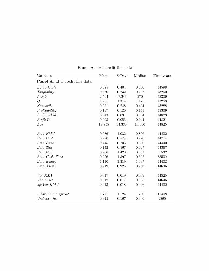
Panel A: LPC credit line data

Variables Mean StDev Median Firm-years

Panel A: LPC credit line data

LC-to-Cash 0.325 0.404 0.000 44598Tangibility 0.350 0.232 0.297 43250Assets 2,594 17,246 270 43309Q 1.961 1.314 1.475 43288Networth 0.381 0.248 0.404 43288Profitability 0.137 0.120 0.141 43309IndSalesVol 0.043 0.031 0.034 44823ProfitVol 0.063 0.053 0.044 44821Age 18.855 14.339 14.000 44825

Beta KMV 0.986 1.032 0.856 44402Beta Cash 0.970 0.574 0.920 44714Beta Bank 0.445 0.703 0.390 44440Beta Tail 0.742 0.567 0.697 44367Beta Gap 0.906 1.420 0.681 35532Beta Cash Flow 0.926 1.397 0.697 35532Beta Equity 1.110 1.319 1.037 44402Beta Asset 0.919 0.926 0.756 14646

Var KMV 0.017 0.019 0.009 44825Var Asset 0.012 0.017 0.005 14646SysVar KMV 0.013 0.018 0.006 44402

All-in drawn spread 1.771 1.124 1.750 11408Undrawn fee 0.315 0.167 0.300 9865

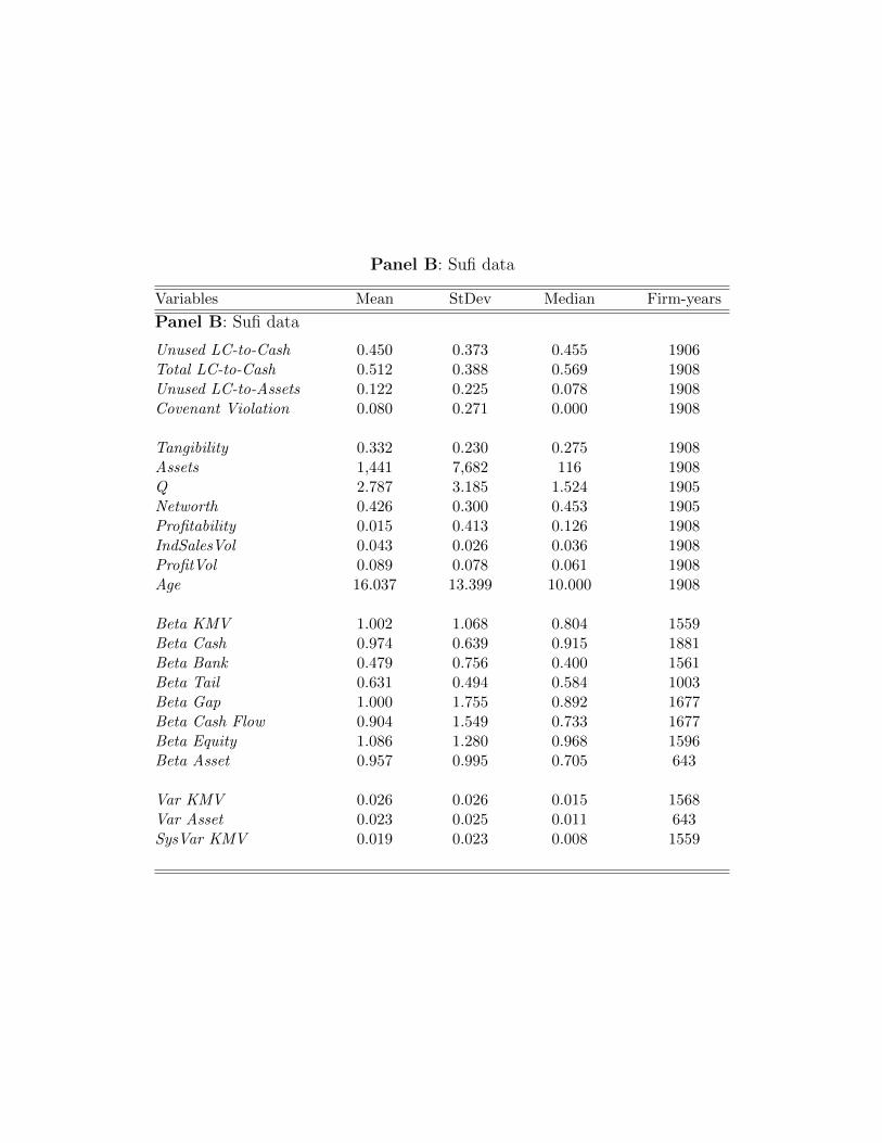
Panel B: Sufi data

Variables Mean StDev Median Firm-years

Panel B: Sufi data

Unused LC-to-Cash 0.450 0.373 0.455 1906Total LC-to-Cash 0.512 0.388 0.569 1908Unused LC-to-Assets 0.122 0.225 0.078 1908Covenant Violation 0.080 0.271 0.000 1908

Tangibility 0.332 0.230 0.275 1908Assets 1,441 7,682 116 1908Q 2.787 3.185 1.524 1905Networth 0.426 0.300 0.453 1905Profitability 0.015 0.413 0.126 1908IndSalesVol 0.043 0.026 0.036 1908ProfitVol 0.089 0.078 0.061 1908Age 16.037 13.399 10.000 1908

Beta KMV 1.002 1.068 0.804 1559Beta Cash 0.974 0.639 0.915 1881Beta Bank 0.479 0.756 0.400 1561Beta Tail 0.631 0.494 0.584 1003Beta Gap 1.000 1.755 0.892 1677Beta Cash Flow 0.904 1.549 0.733 1677Beta Equity 1.086 1.280 0.968 1596Beta Asset 0.957 0.995 0.705 643

Var KMV 0.026 0.026 0.015 1568Var Asset 0.023 0.025 0.011 643SysVar KMV 0.019 0.023 0.008 1559

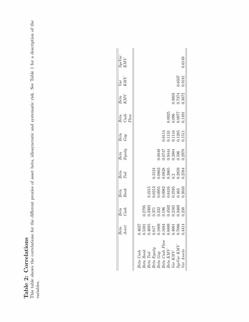
Tab

le2:

Corr

ela

tion

sT

his

tab

lesh

ows

the

corr

elat

ion

sfo

rth

ed

iffer

ent

pro

xie

sof

asse

tb

eta,

idio

syn

crat

ican

dsy

stem

ati

cri

sk.

See

Tab

le1

for

ad

escr

ipti

on

of

the

vari

ab

les.

Bet

aA

sset

Bet

aC

ash

Bet

aB

an

kB

eta

Tail

Bet

aE

quit

yB

eta

Gap

Bet

aC

ash

Flo

w

Bet

aK

MV

Var

KM

VS

ysV

ar

KM

V

Bet

aC

ash

0.46

27B

eta

Ban

k0.

5591

0.27

95B

eta

Tail

0.46

850.

3302

0.2

215

Bet

aE

quit

y0.

817

0.37

10.6

213

0.3

124

Bet

aG

ap

0.18

090.

232

0.0

955

0.0

863

0.0

849

Bet

aC

ash

Flo

w0.

1684

0.19

60.0

982

0.0

828

0.0

747

0.6

114

Bet

aK

MV

0.88

890.

4502

0.6

416

0.3

865

0.9

444

0.1

131

0.0

925

Var

KM

V0.

4001

0.21

650.2

585

0.2

0.2

804

0.1

144

0.0

96

0.3

803

Sys

Var

KM

V0.

7086

0.34

690.4

63

0.2

859

0.5

96

0.1

285

0.0

977

0.7

374

0.6

337

Var

Ass

ets

0.44

140.

238

0.2

633

0.2

584

0.2

978

0.1

511

0.1

491

0.3

872

0.9

181

0.6

149

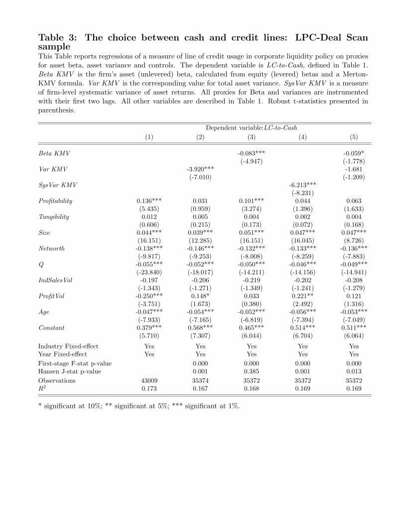
Table 3: The choice between cash and credit lines: LPC-Deal ScansampleThis Table reports regressions of a measure of line of credit usage in corporate liquidity policy on proxiesfor asset beta, asset variance and controls. The dependent variable is LC-to-Cash, defined in Table 1.Beta KMV is the firm’s asset (unlevered) beta, calculated from equity (levered) betas and a Merton-KMV formula. Var KMV is the corresponding value for total asset variance. SysVar KMV is a measureof firm-level systematic variance of asset returns. All proxies for Beta and variances are instrumentedwith their first two lags. All other variables are described in Table 1. Robust t-statistics presented inparenthesis.

Dependent variable:LC-to-Cash

(1) (2) (3) (4) (5)

Beta KMV -0.083*** -0.059*(-4.947) (-1.778)

Var KMV -3.920*** -1.681(-7.010) (-1.209)

SysVar KMV -6.213***(-8.231)

Profitability 0.136*** 0.031 0.101*** 0.044 0.063(5.435) (0.959) (3.274) (1.396) (1.633)

Tangibility 0.012 0.005 0.004 0.002 0.004(0.606) (0.215) (0.173) (0.072) (0.168)

Size 0.044*** 0.039*** 0.051*** 0.047*** 0.047***(16.151) (12.285) (16.151) (16.045) (8.726)

Networth -0.138*** -0.146*** -0.132*** -0.133*** -0.136***(-9.817) (-9.253) (-8.008) (-8.259) (-7.883)

Q -0.055*** -0.052*** -0.050*** -0.046*** -0.049***(-23.840) (-18.017) (-14.211) (-14.156) (-14.941)

IndSalesVol -0.197 -0.206 -0.219 -0.202 -0.208(-1.343) (-1.271) (-1.349) (-1.241) (-1.279)

ProfitVol -0.250*** 0.148* 0.033 0.221** 0.121(-3.751) (1.673) (0.380) (2.492) (1.316)

Age -0.047*** -0.054*** -0.052*** -0.056*** -0.053***(-7.933) (-7.165) (-6.819) (-7.394) (-7.049)

Constant 0.379*** 0.568*** 0.465*** 0.514*** 0.511***(5.710) (7.307) (6.044) (6.704) (6.064)

Industry Fixed-effect Yes Yes Yes Yes YesYear Fixed-effect Yes Yes Yes Yes Yes

First-stage F-stat p-value 0.000 0.000 0.000 0.000Hansen J-stat p-value 0.001 0.385 0.001 0.013

Observations 43009 35374 35372 35372 35372R2 0.173 0.167 0.168 0.169 0.169

* significant at 10%; ** significant at 5%; *** significant at 1%.

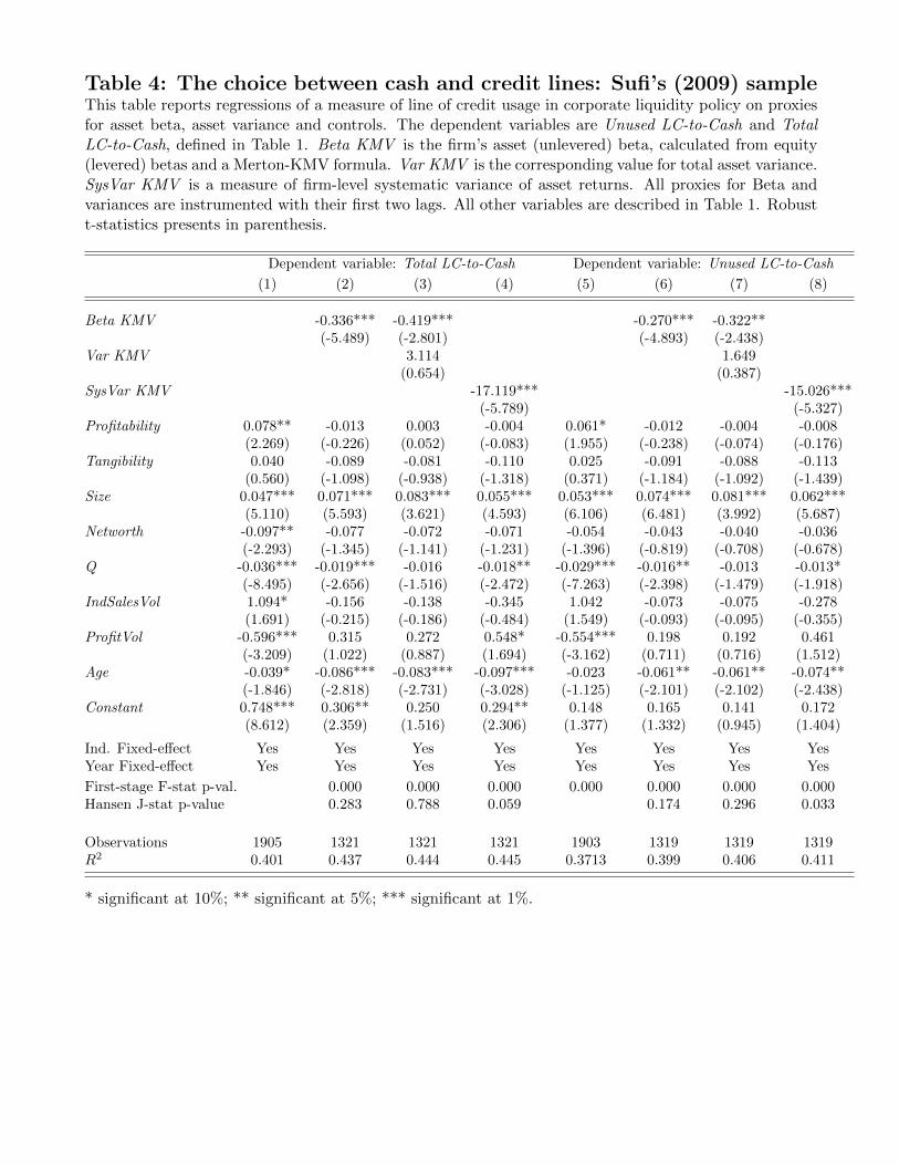
Table 4: The choice between cash and credit lines: Sufi’s (2009) sampleThis table reports regressions of a measure of line of credit usage in corporate liquidity policy on proxiesfor asset beta, asset variance and controls. The dependent variables are Unused LC-to-Cash and TotalLC-to-Cash, defined in Table 1. Beta KMV is the firm’s asset (unlevered) beta, calculated from equity(levered) betas and a Merton-KMV formula. Var KMV is the corresponding value for total asset variance.SysVar KMV is a measure of firm-level systematic variance of asset returns. All proxies for Beta andvariances are instrumented with their first two lags. All other variables are described in Table 1. Robustt-statistics presents in parenthesis.

Dependent variable: Total LC-to-Cash Dependent variable: Unused LC-to-Cash

(1) (2) (3) (4) (5) (6) (7) (8)

Beta KMV -0.336*** -0.419*** -0.270*** -0.322**(-5.489) (-2.801) (-4.893) (-2.438)

Var KMV 3.114 1.649(0.654) (0.387)

SysVar KMV -17.119*** -15.026***(-5.789) (-5.327)

Profitability 0.078** -0.013 0.003 -0.004 0.061* -0.012 -0.004 -0.008(2.269) (-0.226) (0.052) (-0.083) (1.955) (-0.238) (-0.074) (-0.176)

Tangibility 0.040 -0.089 -0.081 -0.110 0.025 -0.091 -0.088 -0.113(0.560) (-1.098) (-0.938) (-1.318) (0.371) (-1.184) (-1.092) (-1.439)

Size 0.047*** 0.071*** 0.083*** 0.055*** 0.053*** 0.074*** 0.081*** 0.062***(5.110) (5.593) (3.621) (4.593) (6.106) (6.481) (3.992) (5.687)

Networth -0.097** -0.077 -0.072 -0.071 -0.054 -0.043 -0.040 -0.036(-2.293) (-1.345) (-1.141) (-1.231) (-1.396) (-0.819) (-0.708) (-0.678)

Q -0.036*** -0.019*** -0.016 -0.018** -0.029*** -0.016** -0.013 -0.013*(-8.495) (-2.656) (-1.516) (-2.472) (-7.263) (-2.398) (-1.479) (-1.918)

IndSalesVol 1.094* -0.156 -0.138 -0.345 1.042 -0.073 -0.075 -0.278(1.691) (-0.215) (-0.186) (-0.484) (1.549) (-0.093) (-0.095) (-0.355)

ProfitVol -0.596*** 0.315 0.272 0.548* -0.554*** 0.198 0.192 0.461(-3.209) (1.022) (0.887) (1.694) (-3.162) (0.711) (0.716) (1.512)

Age -0.039* -0.086*** -0.083*** -0.097*** -0.023 -0.061** -0.061** -0.074**(-1.846) (-2.818) (-2.731) (-3.028) (-1.125) (-2.101) (-2.102) (-2.438)

Constant 0.748*** 0.306** 0.250 0.294** 0.148 0.165 0.141 0.172(8.612) (2.359) (1.516) (2.306) (1.377) (1.332) (0.945) (1.404)

Ind. Fixed-effect Yes Yes Yes Yes Yes Yes Yes YesYear Fixed-effect Yes Yes Yes Yes Yes Yes Yes Yes

First-stage F-stat p-val. 0.000 0.000 0.000 0.000 0.000 0.000 0.000Hansen J-stat p-value 0.283 0.788 0.059 0.174 0.296 0.033

Observations 1905 1321 1321 1321 1903 1319 1319 1319R2 0.401 0.437 0.444 0.445 0.3713 0.399 0.406 0.411


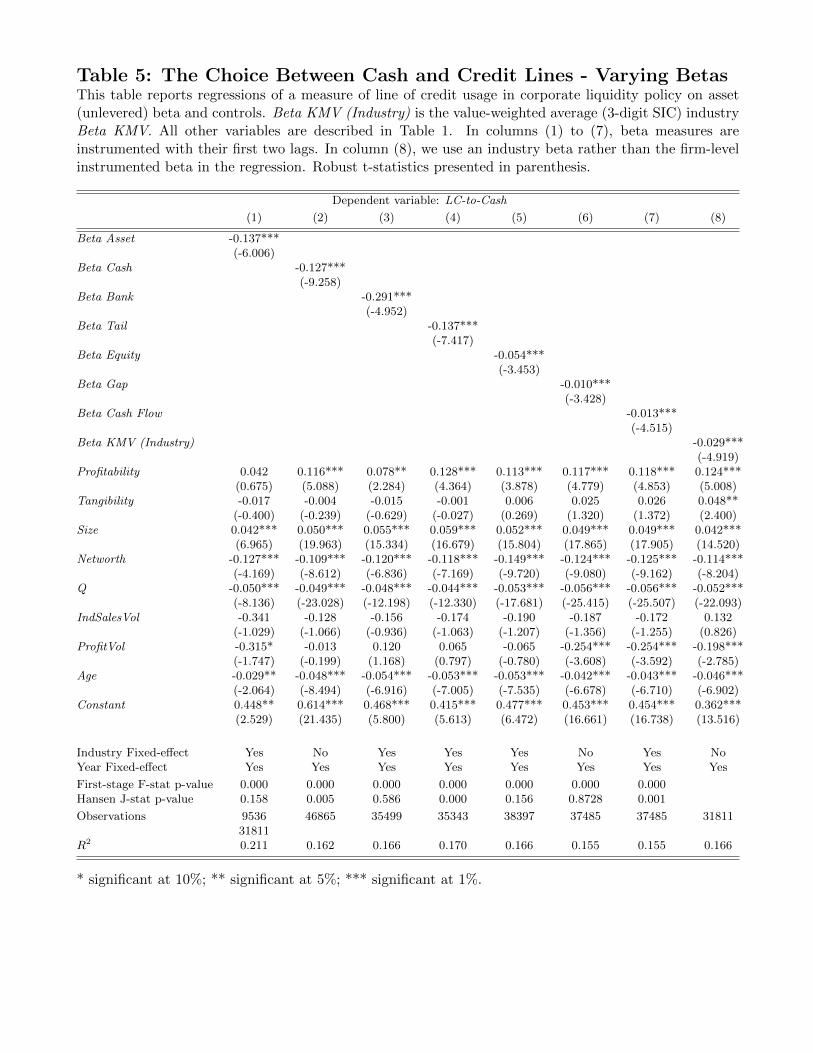
Table 5: The Choice Between Cash and Credit Lines - Varying BetasThis table reports regressions of a measure of line of credit usage in corporate liquidity policy on asset(unlevered) beta and controls. Beta KMV (Industry) is the value-weighted average (3-digit SIC) industryBeta KMV. All other variables are described in Table 1. In columns (1) to (7), beta measures areinstrumented with their first two lags. In column (8), we use an industry beta rather than the firm-levelinstrumented beta in the regression. Robust t-statistics presented in parenthesis.

Dependent variable: LC-to-Cash

(1) (2) (3) (4) (5) (6) (7) (8)

Beta Asset -0.137***(-6.006)

Beta Cash -0.127***(-9.258)

Beta Bank -0.291***(-4.952)

Beta Tail -0.137***(-7.417)

Beta Equity -0.054***(-3.453)

Beta Gap -0.010***(-3.428)

Beta Cash Flow -0.013***(-4.515)

Beta KMV (Industry) -0.029***(-4.919)

Profitability 0.042 0.116*** 0.078** 0.128*** 0.113*** 0.117*** 0.118*** 0.124***(0.675) (5.088) (2.284) (4.364) (3.878) (4.779) (4.853) (5.008)

Tangibility -0.017 -0.004 -0.015 -0.001 0.006 0.025 0.026 0.048**(-0.400) (-0.239) (-0.629) (-0.027) (0.269) (1.320) (1.372) (2.400)

Size 0.042*** 0.050*** 0.055*** 0.059*** 0.052*** 0.049*** 0.049*** 0.042***(6.965) (19.963) (15.334) (16.679) (15.804) (17.865) (17.905) (14.520)

Networth -0.127*** -0.109*** -0.120*** -0.118*** -0.149*** -0.124*** -0.125*** -0.114***(-4.169) (-8.612) (-6.836) (-7.169) (-9.720) (-9.080) (-9.162) (-8.204)

Q -0.050*** -0.049*** -0.048*** -0.044*** -0.053*** -0.056*** -0.056*** -0.052***(-8.136) (-23.028) (-12.198) (-12.330) (-17.681) (-25.415) (-25.507) (-22.093)

IndSalesVol -0.341 -0.128 -0.156 -0.174 -0.190 -0.187 -0.172 0.132(-1.029) (-1.066) (-0.936) (-1.063) (-1.207) (-1.356) (-1.255) (0.826)

ProfitVol -0.315* -0.013 0.120 0.065 -0.065 -0.254*** -0.254*** -0.198***(-1.747) (-0.199) (1.168) (0.797) (-0.780) (-3.608) (-3.592) (-2.785)

Age -0.029** -0.048*** -0.054*** -0.053*** -0.053*** -0.042*** -0.043*** -0.046***(-2.064) (-8.494) (-6.916) (-7.005) (-7.535) (-6.678) (-6.710) (-6.902)

Constant 0.448** 0.614*** 0.468*** 0.415*** 0.477*** 0.453*** 0.454*** 0.362***(2.529) (21.435) (5.800) (5.613) (6.472) (16.661) (16.738) (13.516)

Industry Fixed-effect Yes No Yes Yes Yes No Yes NoYear Fixed-effect Yes Yes Yes Yes Yes Yes Yes Yes

First-stage F-stat p-value 0.000 0.000 0.000 0.000 0.000 0.000 0.000Hansen J-stat p-value 0.158 0.005 0.586 0.000 0.156 0.8728 0.001

Observations 9536 46865 35499 35343 38397 37485 37485 3181131811

R2 0.211 0.162 0.166 0.170 0.166 0.155 0.155 0.166


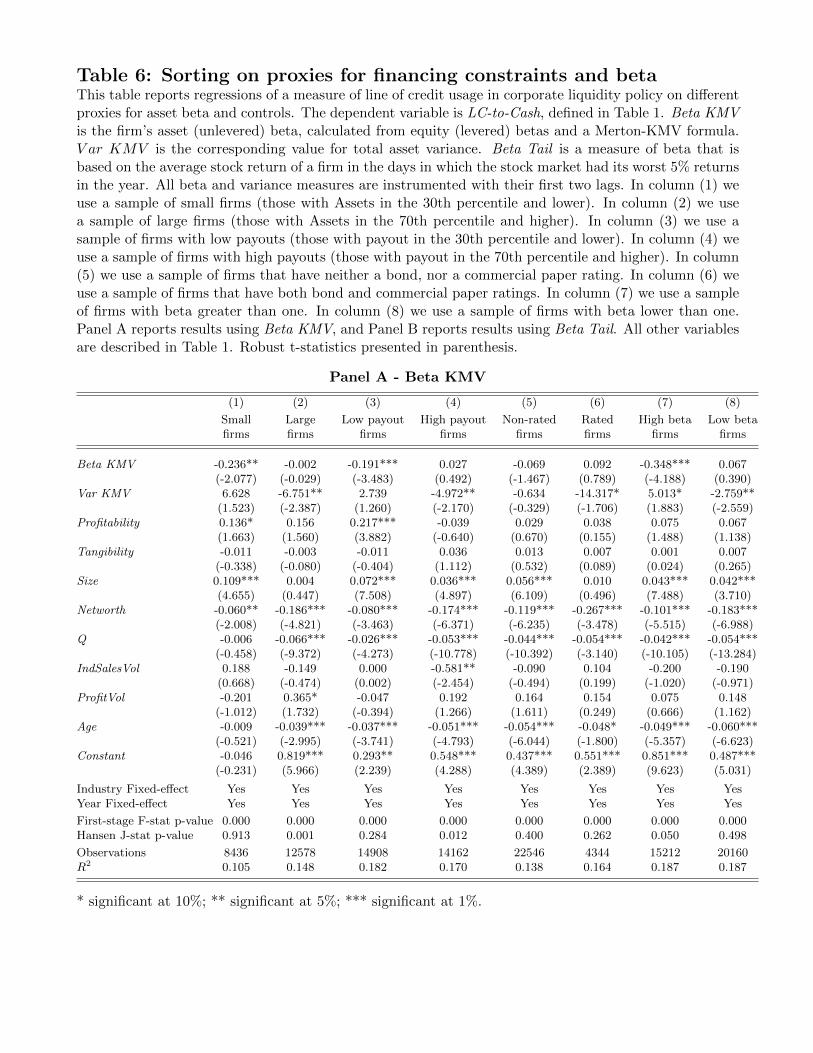
Table 6: Sorting on proxies for financing constraints and betaThis table reports regressions of a measure of line of credit usage in corporate liquidity policy on differentproxies for asset beta and controls. The dependent variable is LC-to-Cash, defined in Table 1. Beta KMVis the firm’s asset (unlevered) beta, calculated from equity (levered) betas and a Merton-KMV formula.V ar KMV is the corresponding value for total asset variance. Beta Tail is a measure of beta that isbased on the average stock return of a firm in the days in which the stock market had its worst 5% returnsin the year. All beta and variance measures are instrumented with their first two lags. In column (1) weuse a sample of small firms (those with Assets in the 30th percentile and lower). In column (2) we usea sample of large firms (those with Assets in the 70th percentile and higher). In column (3) we use asample of firms with low payouts (those with payout in the 30th percentile and lower). In column (4) weuse a sample of firms with high payouts (those with payout in the 70th percentile and higher). In column(5) we use a sample of firms that have neither a bond, nor a commercial paper rating. In column (6) weuse a sample of firms that have both bond and commercial paper ratings. In column (7) we use a sampleof firms with beta greater than one. In column (8) we use a sample of firms with beta lower than one.Panel A reports results using Beta KMV, and Panel B reports results using Beta Tail. All other variablesare described in Table 1. Robust t-statistics presented in parenthesis.

Panel A - Beta KMV

(1) (2) (3) (4) (5) (6) (7) (8)

Small Large Low payout High payout Non-rated Rated High beta Low betafirms firms firms firms firms firms firms firms

Beta KMV -0.236** -0.002 -0.191*** 0.027 -0.069 0.092 -0.348*** 0.067(-2.077) (-0.029) (-3.483) (0.492) (-1.467) (0.789) (-4.188) (0.390)

Var KMV 6.628 -6.751** 2.739 -4.972** -0.634 -14.317* 5.013* -2.759**(1.523) (-2.387) (1.260) (-2.170) (-0.329) (-1.706) (1.883) (-2.559)

Profitability 0.136* 0.156 0.217*** -0.039 0.029 0.038 0.075 0.067(1.663) (1.560) (3.882) (-0.640) (0.670) (0.155) (1.488) (1.138)

Tangibility -0.011 -0.003 -0.011 0.036 0.013 0.007 0.001 0.007(-0.338) (-0.080) (-0.404) (1.112) (0.532) (0.089) (0.024) (0.265)

Size 0.109*** 0.004 0.072*** 0.036*** 0.056*** 0.010 0.043*** 0.042***(4.655) (0.447) (7.508) (4.897) (6.109) (0.496) (7.488) (3.710)

Networth -0.060** -0.186*** -0.080*** -0.174*** -0.119*** -0.267*** -0.101*** -0.183***(-2.008) (-4.821) (-3.463) (-6.371) (-6.235) (-3.478) (-5.515) (-6.988)

Q -0.006 -0.066*** -0.026*** -0.053*** -0.044*** -0.054*** -0.042*** -0.054***(-0.458) (-9.372) (-4.273) (-10.778) (-10.392) (-3.140) (-10.105) (-13.284)

IndSalesVol 0.188 -0.149 0.000 -0.581** -0.090 0.104 -0.200 -0.190(0.668) (-0.474) (0.002) (-2.454) (-0.494) (0.199) (-1.020) (-0.971)

ProfitVol -0.201 0.365* -0.047 0.192 0.164 0.154 0.075 0.148(-1.012) (1.732) (-0.394) (1.266) (1.611) (0.249) (0.666) (1.162)

Age -0.009 -0.039*** -0.037*** -0.051*** -0.054*** -0.048* -0.049*** -0.060***(-0.521) (-2.995) (-3.741) (-4.793) (-6.044) (-1.800) (-5.357) (-6.623)

Constant -0.046 0.819*** 0.293** 0.548*** 0.437*** 0.551*** 0.851*** 0.487***(-0.231) (5.966) (2.239) (4.288) (4.389) (2.389) (9.623) (5.031)

Industry Fixed-effect Yes Yes Yes Yes Yes Yes Yes YesYear Fixed-effect Yes Yes Yes Yes Yes Yes Yes Yes

First-stage F-stat p-value 0.000 0.000 0.000 0.000 0.000 0.000 0.000 0.000Hansen J-stat p-value 0.913 0.001 0.284 0.012 0.400 0.262 0.050 0.498

Observations 8436 12578 14908 14162 22546 4344 15212 20160R2 0.105 0.148 0.182 0.170 0.138 0.164 0.187 0.187


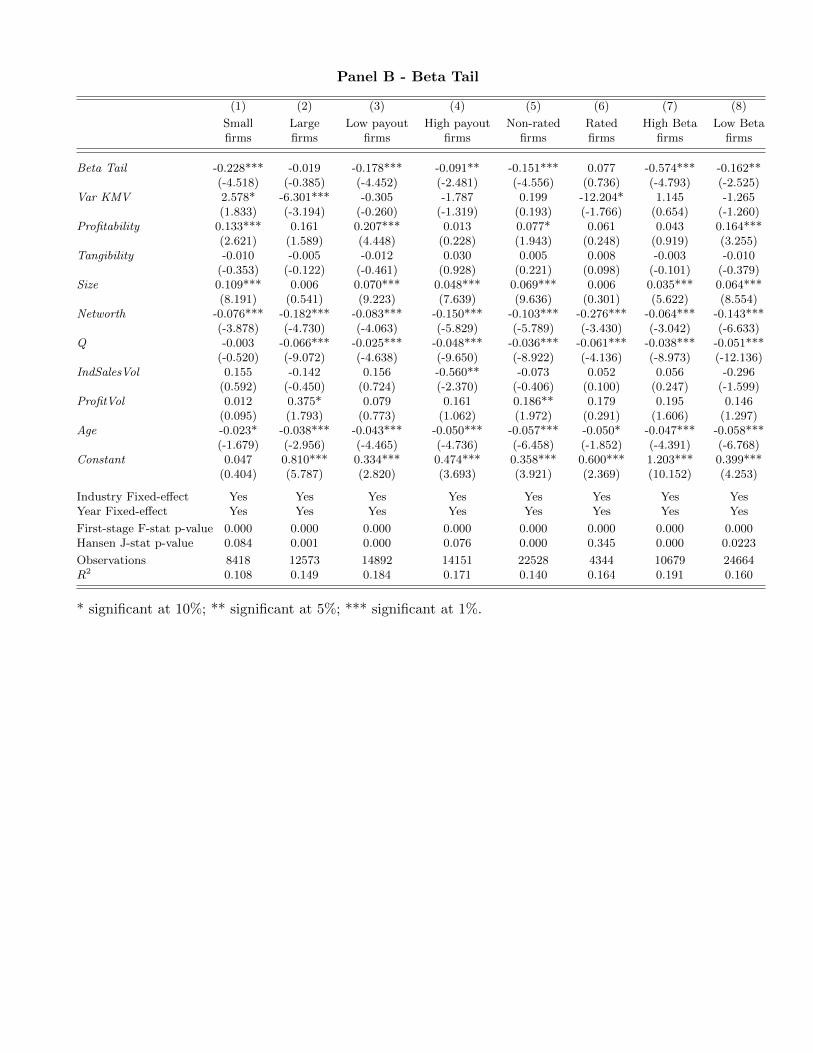
Panel B - Beta Tail

(1) (2) (3) (4) (5) (6) (7) (8)

Small Large Low payout High payout Non-rated Rated High Beta Low Betafirms firms firms firms firms firms firms firms

Beta Tail -0.228*** -0.019 -0.178*** -0.091** -0.151*** 0.077 -0.574*** -0.162**(-4.518) (-0.385) (-4.452) (-2.481) (-4.556) (0.736) (-4.793) (-2.525)

Var KMV 2.578* -6.301*** -0.305 -1.787 0.199 -12.204* 1.145 -1.265(1.833) (-3.194) (-0.260) (-1.319) (0.193) (-1.766) (0.654) (-1.260)

Profitability 0.133*** 0.161 0.207*** 0.013 0.077* 0.061 0.043 0.164***(2.621) (1.589) (4.448) (0.228) (1.943) (0.248) (0.919) (3.255)

Tangibility -0.010 -0.005 -0.012 0.030 0.005 0.008 -0.003 -0.010(-0.353) (-0.122) (-0.461) (0.928) (0.221) (0.098) (-0.101) (-0.379)

Size 0.109*** 0.006 0.070*** 0.048*** 0.069*** 0.006 0.035*** 0.064***(8.191) (0.541) (9.223) (7.639) (9.636) (0.301) (5.622) (8.554)

Networth -0.076*** -0.182*** -0.083*** -0.150*** -0.103*** -0.276*** -0.064*** -0.143***(-3.878) (-4.730) (-4.063) (-5.829) (-5.789) (-3.430) (-3.042) (-6.633)

Q -0.003 -0.066*** -0.025*** -0.048*** -0.036*** -0.061*** -0.038*** -0.051***(-0.520) (-9.072) (-4.638) (-9.650) (-8.922) (-4.136) (-8.973) (-12.136)

IndSalesVol 0.155 -0.142 0.156 -0.560** -0.073 0.052 0.056 -0.296(0.592) (-0.450) (0.724) (-2.370) (-0.406) (0.100) (0.247) (-1.599)

ProfitVol 0.012 0.375* 0.079 0.161 0.186** 0.179 0.195 0.146(0.095) (1.793) (0.773) (1.062) (1.972) (0.291) (1.606) (1.297)

Age -0.023* -0.038*** -0.043*** -0.050*** -0.057*** -0.050* -0.047*** -0.058***(-1.679) (-2.956) (-4.465) (-4.736) (-6.458) (-1.852) (-4.391) (-6.768)

Constant 0.047 0.810*** 0.334*** 0.474*** 0.358*** 0.600*** 1.203*** 0.399***(0.404) (5.787) (2.820) (3.693) (3.921) (2.369) (10.152) (4.253)


First-stage F-stat p-value 0.000 0.000 0.000 0.000 0.000 0.000 0.000 0.000Hansen J-stat p-value 0.084 0.001 0.000 0.076 0.000 0.345 0.000 0.0223

Observations 8418 12573 14892 14151 22528 4344 10679 24664R2 0.108 0.149 0.184 0.171 0.140 0.164 0.191 0.160


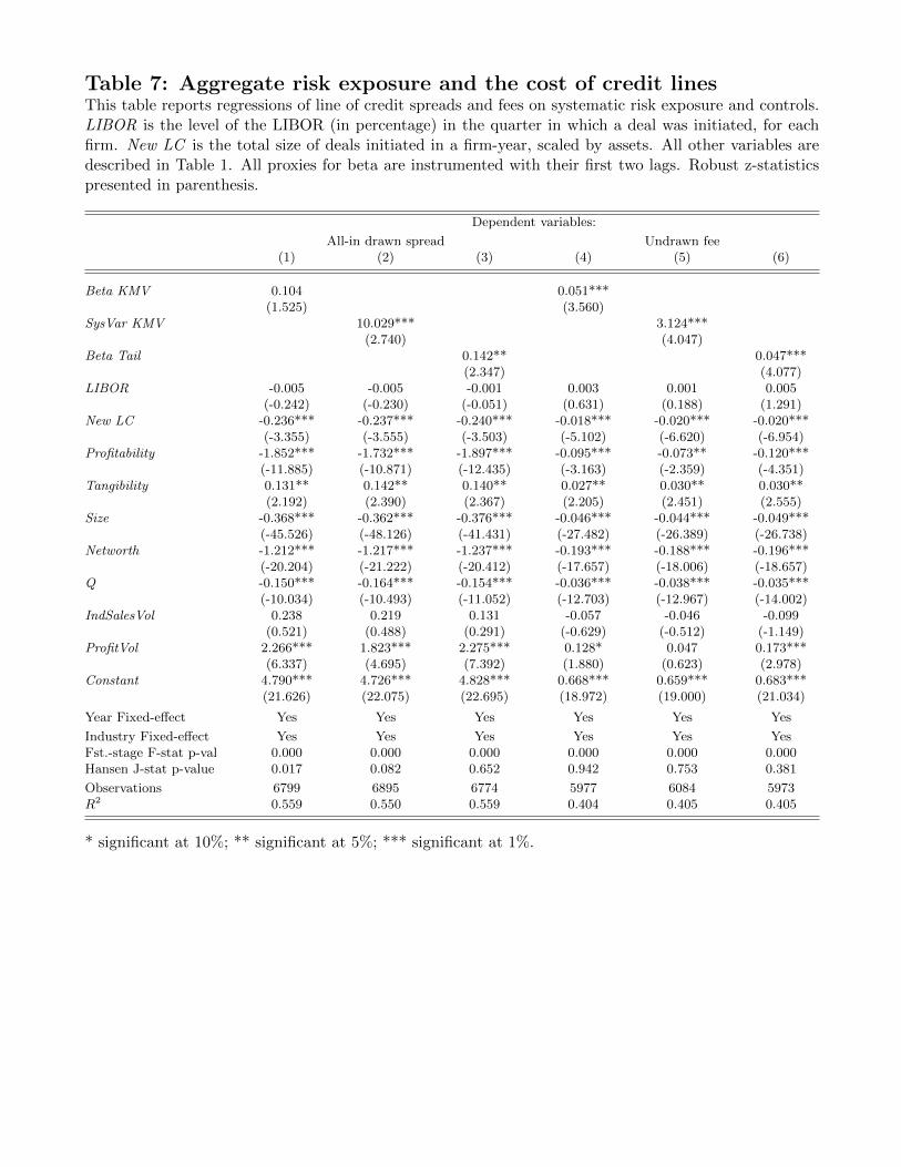
Table 7: Aggregate risk exposure and the cost of credit linesThis table reports regressions of line of credit spreads and fees on systematic risk exposure and controls.LIBOR is the level of the LIBOR (in percentage) in the quarter in which a deal was initiated, for eachfirm. New LC is the total size of deals initiated in a firm-year, scaled by assets. All other variables aredescribed in Table 1. All proxies for beta are instrumented with their first two lags. Robust z-statisticspresented in parenthesis.

Dependent variables:

All-in drawn spread Undrawn fee(1) (2) (3) (4) (5) (6)

Beta KMV 0.104 0.051***(1.525) (3.560)

SysVar KMV 10.029*** 3.124***(2.740) (4.047)

Beta Tail 0.142** 0.047***(2.347) (4.077)

LIBOR -0.005 -0.005 -0.001 0.003 0.001 0.005(-0.242) (-0.230) (-0.051) (0.631) (0.188) (1.291)

New LC -0.236*** -0.237*** -0.240*** -0.018*** -0.020*** -0.020***(-3.355) (-3.555) (-3.503) (-5.102) (-6.620) (-6.954)

Profitability -1.852*** -1.732*** -1.897*** -0.095*** -0.073** -0.120***(-11.885) (-10.871) (-12.435) (-3.163) (-2.359) (-4.351)

Tangibility 0.131** 0.142** 0.140** 0.027** 0.030** 0.030**(2.192) (2.390) (2.367) (2.205) (2.451) (2.555)

Size -0.368*** -0.362*** -0.376*** -0.046*** -0.044*** -0.049***(-45.526) (-48.126) (-41.431) (-27.482) (-26.389) (-26.738)

Networth -1.212*** -1.217*** -1.237*** -0.193*** -0.188*** -0.196***(-20.204) (-21.222) (-20.412) (-17.657) (-18.006) (-18.657)

Q -0.150*** -0.164*** -0.154*** -0.036*** -0.038*** -0.035***(-10.034) (-10.493) (-11.052) (-12.703) (-12.967) (-14.002)

IndSalesVol 0.238 0.219 0.131 -0.057 -0.046 -0.099(0.521) (0.488) (0.291) (-0.629) (-0.512) (-1.149)

ProfitVol 2.266*** 1.823*** 2.275*** 0.128* 0.047 0.173***(6.337) (4.695) (7.392) (1.880) (0.623) (2.978)

Constant 4.790*** 4.726*** 4.828*** 0.668*** 0.659*** 0.683***(21.626) (22.075) (22.695) (18.972) (19.000) (21.034)

Year Fixed-effect Yes Yes Yes Yes Yes Yes

Industry Fixed-effect Yes Yes Yes Yes Yes YesFst.-stage F-stat p-val 0.000 0.000 0.000 0.000 0.000 0.000Hansen J-stat p-value 0.017 0.082 0.652 0.942 0.753 0.381

Observations 6799 6895 6774 5977 6084 5973R2 0.559 0.550 0.559 0.404 0.405 0.405


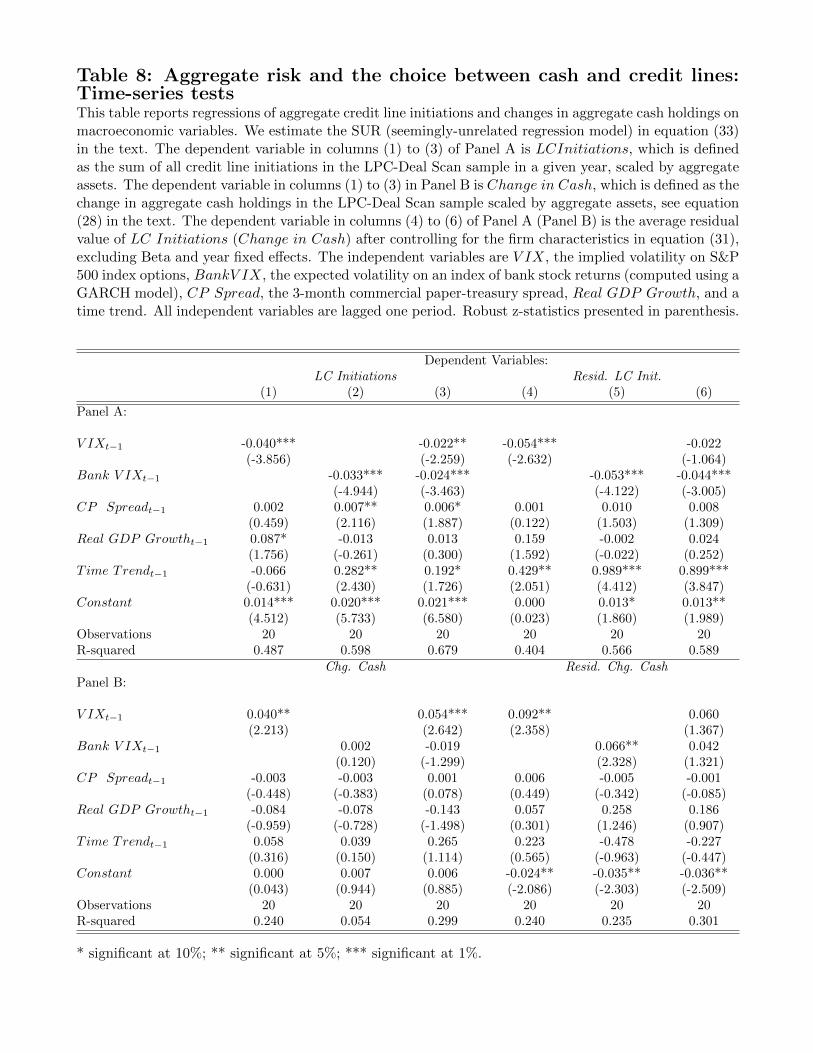
Table 8: Aggregate risk and the choice between cash and credit lines:Time-series testsThis table reports regressions of aggregate credit line initiations and changes in aggregate cash holdings onmacroeconomic variables. We estimate the SUR (seemingly-unrelated regression model) in equation (33)in the text. The dependent variable in columns (1) to (3) of Panel A is LCInitiations, which is definedas the sum of all credit line initiations in the LPC-Deal Scan sample in a given year, scaled by aggregateassets. The dependent variable in columns (1) to (3) in Panel B is Change in Cash, which is defined as thechange in aggregate cash holdings in the LPC-Deal Scan sample scaled by aggregate assets, see equation(28) in the text. The dependent variable in columns (4) to (6) of Panel A (Panel B) is the average residualvalue of LC Initiations (Change in Cash) after controlling for the firm characteristics in equation (31),excluding Beta and year fixed effects. The independent variables are V IX, the implied volatility on S&P500 index options, BankV IX, the expected volatility on an index of bank stock returns (computed using aGARCH model), CP Spread, the 3-month commercial paper-treasury spread, Real GDP Growth, and atime trend. All independent variables are lagged one period. Robust z-statistics presented in parenthesis.

Dependent Variables:LC Initiations Resid. LC Init.

(1) (2) (3) (4) (5) (6)

Panel A:

V IXt−1 -0.040*** -0.022** -0.054*** -0.022(-3.856) (-2.259) (-2.632) (-1.064)

Bank V IXt−1 -0.033*** -0.024*** -0.053*** -0.044***(-4.944) (-3.463) (-4.122) (-3.005)

CP Spreadt−1 0.002 0.007** 0.006* 0.001 0.010 0.008(0.459) (2.116) (1.887) (0.122) (1.503) (1.309)

Real GDP Growtht−1 0.087* -0.013 0.013 0.159 -0.002 0.024(1.756) (-0.261) (0.300) (1.592) (-0.022) (0.252)

Time Trendt−1 -0.066 0.282** 0.192* 0.429** 0.989*** 0.899***(-0.631) (2.430) (1.726) (2.051) (4.412) (3.847)

Constant 0.014*** 0.020*** 0.021*** 0.000 0.013* 0.013**(4.512) (5.733) (6.580) (0.023) (1.860) (1.989)

Observations 20 20 20 20 20 20R-squared 0.487 0.598 0.679 0.404 0.566 0.589

Chg. Cash Resid. Chg. CashPanel B:

V IXt−1 0.040** 0.054*** 0.092** 0.060(2.213) (2.642) (2.358) (1.367)

Bank V IXt−1 0.002 -0.019 0.066** 0.042(0.120) (-1.299) (2.328) (1.321)

CP Spreadt−1 -0.003 -0.003 0.001 0.006 -0.005 -0.001(-0.448) (-0.383) (0.078) (0.449) (-0.342) (-0.085)

Real GDP Growtht−1 -0.084 -0.078 -0.143 0.057 0.258 0.186(-0.959) (-0.728) (-1.498) (0.301) (1.246) (0.907)

Time Trendt−1 0.058 0.039 0.265 0.223 -0.478 -0.227(0.316) (0.150) (1.114) (0.565) (-0.963) (-0.447)

Constant 0.000 0.007 0.006 -0.024** -0.035** -0.036**(0.043) (0.944) (0.885) (-2.086) (-2.303) (-2.509)



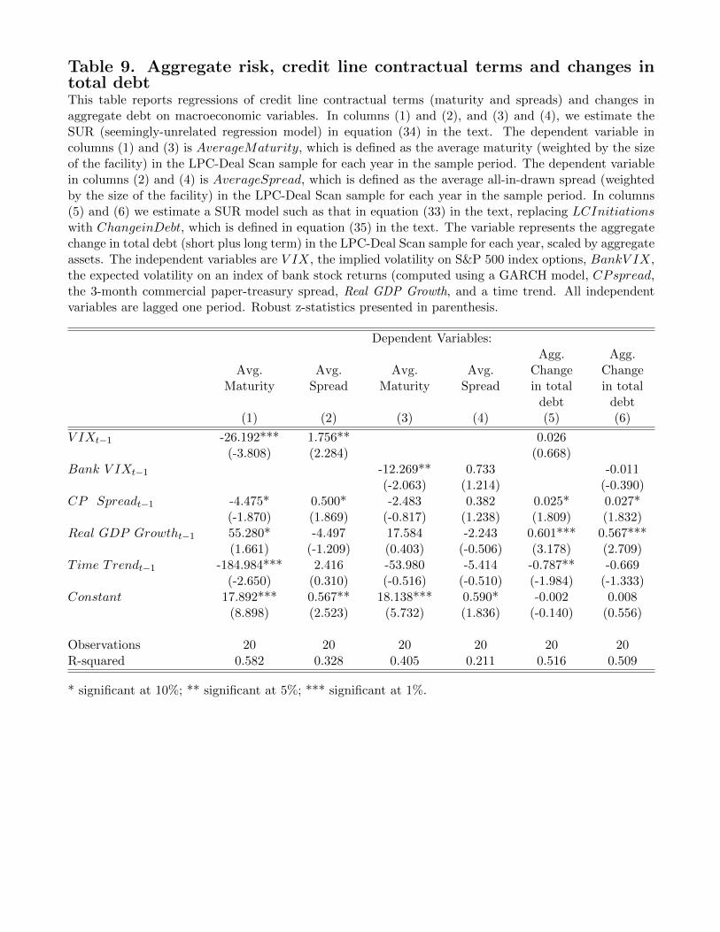
Table 9. Aggregate risk, credit line contractual terms and changes intotal debtThis table reports regressions of credit line contractual terms (maturity and spreads) and changes inaggregate debt on macroeconomic variables. In columns (1) and (2), and (3) and (4), we estimate theSUR (seemingly-unrelated regression model) in equation (34) in the text. The dependent variable incolumns (1) and (3) is AverageMaturity, which is defined as the average maturity (weighted by the sizeof the facility) in the LPC-Deal Scan sample for each year in the sample period. The dependent variablein columns (2) and (4) is AverageSpread, which is defined as the average all-in-drawn spread (weightedby the size of the facility) in the LPC-Deal Scan sample for each year in the sample period. In columns(5) and (6) we estimate a SUR model such as that in equation (33) in the text, replacing LCInitiationswith ChangeinDebt, which is defined in equation (35) in the text. The variable represents the aggregatechange in total debt (short plus long term) in the LPC-Deal Scan sample for each year, scaled by aggregateassets. The independent variables are V IX, the implied volatility on S&P 500 index options, BankV IX,the expected volatility on an index of bank stock returns (computed using a GARCH model, CPspread,the 3-month commercial paper-treasury spread, Real GDP Growth, and a time trend. All independentvariables are lagged one period. Robust z-statistics presented in parenthesis.

Dependent Variables:

Avg.Maturity

Avg.Spread

Avg.Maturity

Avg.Spread

Agg.Changein total

debt

Agg.Changein total

debt(1) (2) (3) (4) (5) (6)

V IXt−1 -26.192*** 1.756** 0.026(-3.808) (2.284) (0.668)

Bank V IXt−1 -12.269** 0.733 -0.011(-2.063) (1.214) (-0.390)

CP Spreadt−1 -4.475* 0.500* -2.483 0.382 0.025* 0.027*(-1.870) (1.869) (-0.817) (1.238) (1.809) (1.832)

Real GDP Growtht−1 55.280* -4.497 17.584 -2.243 0.601*** 0.567***(1.661) (-1.209) (0.403) (-0.506) (3.178) (2.709)

Time Trendt−1 -184.984*** 2.416 -53.980 -5.414 -0.787** -0.669(-2.650) (0.310) (-0.516) (-0.510) (-1.984) (-1.333)

Constant 17.892*** 0.567** 18.138*** 0.590* -0.002 0.008(8.898) (2.523) (5.732) (1.836) (-0.140) (0.556)



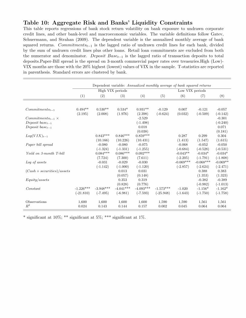
Table 10: Aggregate Risk and Banks’ Liquidity ConstraintsThis table reports regressions of bank stock return volatility on bank exposure to undrawn corporatecredit lines, and other bank-level and macroeconomic variables. The variable definitions follow Gatev,Schuermann, and Strahan (2009). The dependent variable is the annualized monthly average of banksquared returns. Commitmentst−1 is the lagged ratio of undrawn credit lines for each bank, dividedby the sum of undrawn credit lines plus other loans. Retail loan commitments are excluded from boththe numerator and denominator. Deposit Baset−1 is the lagged ratio of transaction deposits to totaldeposits.Paper-Bill spread is the spread on 3-month commercial paper rates over treasuries.High (Low)-VIX months are those with the 20% highest (lowest) values of VIX in the sample. T-statistics are reportedin parenthesis. Standard errors are clustered by bank.

Dependent variable: Annualized monthly average of bank squared returns

High VIX periods Low VIX periods

(1) (2) (3) (4) (5) (6) (7) (8)

Commitmentst−1 0.494** 0.530** 0.534* 0.931** -0.129 0.007 -0.121 -0.057(2.195) (2.008) (1.976) (2.398) (-0.624) (0.032) (-0.509) (-0.142)

Commitmentst−1 × -2.529 -0.301Deposit baset−1 (-1.498) (-0.240)Deposit baset−1 0.018 0.071

(0.038) (0.181)Log(V IX)t−1 0.843*** 0.846*** 0.859*** 0.287 0.299 0.304

(10.166) (10.226) (10.431) (1.413) (1.547) (1.615)Paper bill spread -0.080 -0.080 -0.075 -0.068 -0.052 -0.050

(-1.324) (-1.331) (-1.255) (-0.684) (-0.528) (-0.531)Yield on 3-month T-bill 0.084*** 0.086*** 0.092*** -0.043** -0.034* -0.034*

(7.724) (7.300) (7.611) (-2.205) (-1.791) (-1.808)Log of assets -0.031 -0.029 -0.030 -0.069*** -0.068*** -0.069**

(-1.142) (-1.000) (-1.120) (-2.857) (-2.624) (-2.471)(Cash + securities)/assets 0.013 0.031 0.388 0.383

(0.057) (0.148) (1.353) (1.323)Equity/assets 0.353 0.319 -0.382 -0.389

(0.828) (0.776) (-0.982) (-1.013)Constant -1.226*** -3.948*** -4.041*** -4.093*** -1.573*** -1.020 -1.156* -1.162*

(-21.810) (-7.495) (-6.981) (-7.593) (-25.948) (-1.643) (-1.750) (-1.758)

Observations 1,600 1,600 1,600 1,600 1,590 1,590 1,561 1,561R2 0.024 0.143 0.144 0.157 0.002 0.045 0.064 0.064


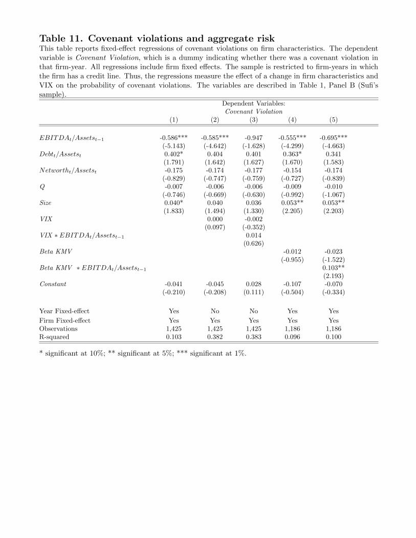
Table 11. Covenant violations and aggregate riskThis table reports fixed-effect regressions of covenant violations on firm characteristics. The dependentvariable is Covenant Violation, which is a dummy indicating whether there was a covenant violation inthat firm-year. All regressions include firm fixed effects. The sample is restricted to firm-years in whichthe firm has a credit line. Thus, the regressions measure the effect of a change in firm characteristics andVIX on the probability of covenant violations. The variables are described in Table 1, Panel B (Sufi’ssample).

Dependent Variables:Covenant Violation

(1) (2) (3) (4) (5)

EBITDAt/Assetst−1 -0.586*** -0.585*** -0.947 -0.555*** -0.695***(-5.143) (-4.642) (-1.628) (-4.299) (-4.663)

Debtt/Assetst 0.402* 0.404 0.401 0.363* 0.341(1.791) (1.642) (1.627) (1.670) (1.583)

Networtht/Assetst -0.175 -0.174 -0.177 -0.154 -0.174(-0.829) (-0.747) (-0.759) (-0.727) (-0.839)

Q -0.007 -0.006 -0.006 -0.009 -0.010(-0.746) (-0.669) (-0.630) (-0.992) (-1.067)

Size 0.040* 0.040 0.036 0.053** 0.053**(1.833) (1.494) (1.330) (2.205) (2.203)

VIX 0.000 -0.002(0.097) (-0.352)

VIX ∗ EBITDAt/Assetst−1 0.014(0.626)

Beta KMV -0.012 -0.023(-0.955) (-1.522)

Beta KMV ∗ EBITDAt/Assetst−1 0.103**(2.193)

Constant -0.041 -0.045 0.028 -0.107 -0.070(-0.210) (-0.208) (0.111) (-0.504) (-0.334)

Year Fixed-effect Yes No No Yes Yes

Firm Fixed-effect Yes Yes Yes Yes YesObservations 1,425 1,425 1,425 1,186 1,186R-squared 0.103 0.382 0.383 0.096 0.100


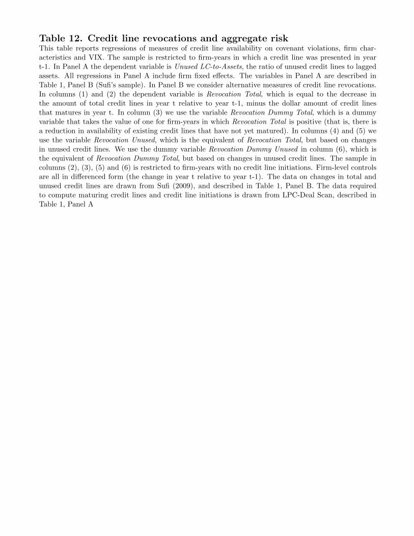
Table 12. Credit line revocations and aggregate riskThis table reports regressions of measures of credit line availability on covenant violations, firm char-acteristics and VIX. The sample is restricted to firm-years in which a credit line was presented in yeart-1. In Panel A the dependent variable is Unused LC-to-Assets, the ratio of unused credit lines to laggedassets. All regressions in Panel A include firm fixed effects. The variables in Panel A are described inTable 1, Panel B (Sufi’s sample). In Panel B we consider alternative measures of credit line revocations.In columns (1) and (2) the dependent variable is Revocation Total, which is equal to the decrease inthe amount of total credit lines in year t relative to year t-1, minus the dollar amount of credit linesthat matures in year t. In column (3) we use the variable Revocation Dummy Total, which is a dummyvariable that takes the value of one for firm-years in which Revocation Total is positive (that is, there isa reduction in availability of existing credit lines that have not yet matured). In columns (4) and (5) weuse the variable Revocation Unused, which is the equivalent of Revocation Total, but based on changesin unused credit lines. We use the dummy variable Revocation Dummy Unused in column (6), which isthe equivalent of Revocation Dummy Total, but based on changes in unused credit lines. The sample incolumns (2), (3), (5) and (6) is restricted to firm-years with no credit line initiations. Firm-level controlsare all in differenced form (the change in year t relative to year t-1). The data on changes in total andunused credit lines are drawn from Sufi (2009), and described in Table 1, Panel B. The data requiredto compute maturing credit lines and credit line initiations is drawn from LPC-Deal Scan, described inTable 1, Panel A

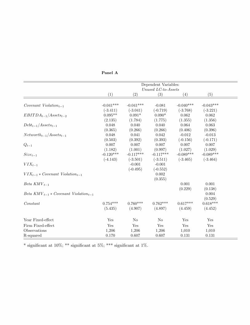
Panel A

Dependent Variables:Unused LC-to-Assets

(1) (2) (3) (4) (5)

Covenant Violationt−1 -0.041*** -0.041*** -0.081 -0.040*** -0.043***(-3.411) (-3.041) (-0.719) (-3.768) (-3.221)

EBITDAt−1/Assetst−2 0.095** 0.091* 0.090* 0.062 0.062(2.135) (1.784) (1.775) (1.355) (1.356)

Debtt−1/Assetst−1 0.048 0.040 0.040 0.064 0.063(0.365) (0.266) (0.266) (0.406) (0.396)

Networtht−1/Assetst−1 0.048 0.041 0.042 -0.012 -0.013(0.503) (0.392) (0.393) (-0.156) (-0.171)

Qt−1 0.007 0.007 0.007 0.007 0.007(1.182) (1.001) (0.997) (1.027) (1.029)

Sizet−1 -0.120*** -0.117*** -0.117*** -0.089*** -0.089***(-4.143) (-3.501) (-3.511) (-3.465) (-3.464)

V IXt−1 -0.001 -0.001(-0.495) (-0.552)

V IXt−1 ∗ Covenant Violationt−1 0.002(0.355)

Beta KMV t−1 0.001 0.001(0.229) (0.138)

Beta KMV t−1 ∗ Covenant Violationt−1 0.004(0.529)

Constant 0.754*** 0.760*** 0.762*** 0.617*** 0.618***(5.435) (4.907) (4.897) (4.459) (4.452)




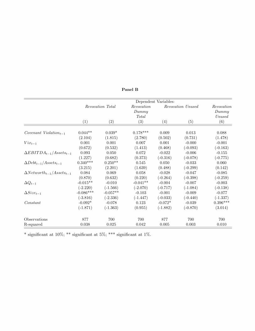
Panel B

Dependent Variables:Revocation Total Revocation

DummyTotal

Revocation Unused RevocationDummyUnused

(1) (2) (3) (4) (5) (6)

Covenant Violationt−1 0.044** 0.039* 0.178*** 0.009 0.013 0.088(2.104) (1.815) (2.780) (0.502) (0.731) (1.478)

V ixt−1 0.001 0.001 0.007 0.001 -0.000 -0.001(0.672) (0.532) (1.413) (0.468) (-0.093) (-0.163)

∆EBITDAt−1/Assetst−1 0.093 0.050 0.072 -0.022 -0.006 -0.155(1.227) (0.682) (0.373) (-0.316) (-0.078) (-0.775)

∆Debtt−1/Assetst−1 0.340*** 0.250** 0.545 0.050 -0.033 0.060(3.215) (2.201) (1.639) (0.488) (-0.299) (0.142)

∆Networtht−1/Assetst−1 0.084 0.069 0.058 -0.028 -0.047 -0.085(0.870) (0.632) (0.220) (-0.264) (-0.398) (-0.259)

∆Qt−1 -0.015** -0.010 -0.041** -0.004 -0.007 -0.003(-2.220) (-1.566) (-2.070) (-0.717) (-1.084) (-0.138)

∆Sizet−1 -0.086*** -0.057** -0.103 -0.001 -0.009 -0.077(-3.816) (-2.336) (-1.447) (-0.033) (-0.440) (-1.337)

Constant -0.092* -0.078 0.123 -0.072* -0.039 0.396***(-1.871) (-1.363) (0.955) (-1.882) (-0.870) (3.014)



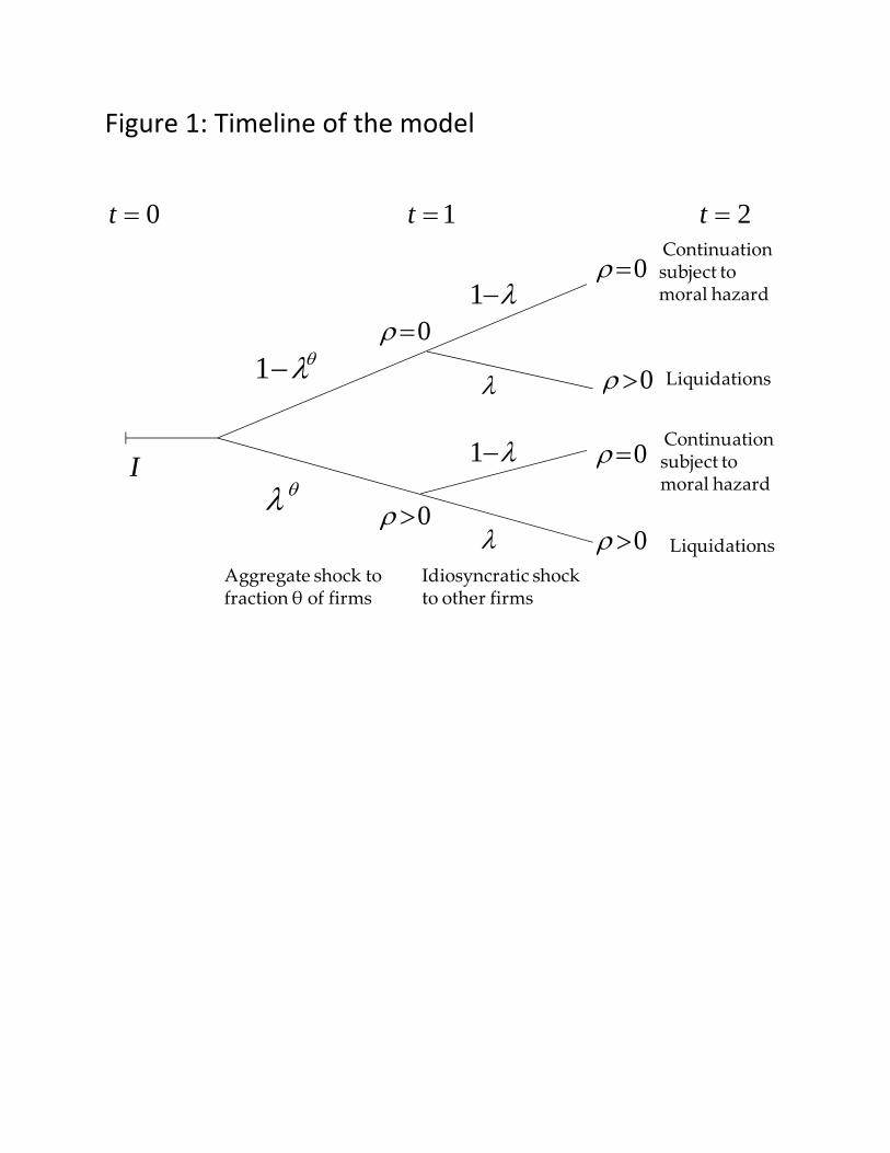
Figure 1: Timeline of the model

0t

I

1

1

1

0

1t

0

0

00

0

Aggregate shock to fraction θ of firms

Idiosyncratic shock to other firms

2t Continuationsubject to moral hazard

Continuationsubject to moral hazard

Liquidations

Liquidations

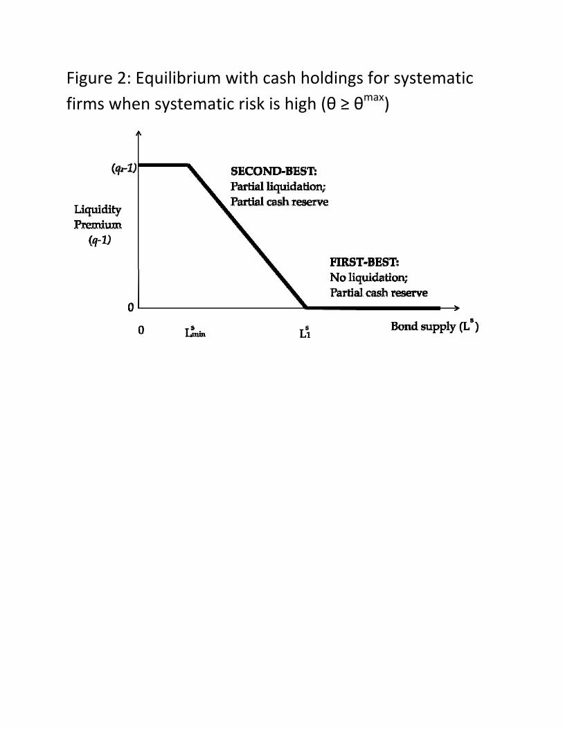
Figure 2: Equilibrium with cash holdings for systematic firms when systematic risk is high (θ ≥ θmax)

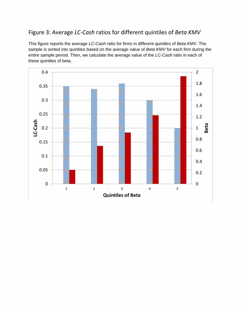
Figure 3: Average LC‐Cash ratios for different quintiles of Beta KMV

This figure reports the average LC-Cash ratio for firms in different quintiles of Beta KMV. The sample is sorted into quintiles based on the average value of Beta KMV for each firm during the entire sample period. Then, we calculate the average value of the LC-Cash ratio in each of these quintiles of beta.

0

0.2

0.4

0.6

0.8

1

1.2

1.4

1.6

1.8

2

0

0.05

0.1

0.15

0.2

0.25

0.3

0.35

0.4

1 2 3 4 5

Beta

LC‐Cash

Quintiles of Beta

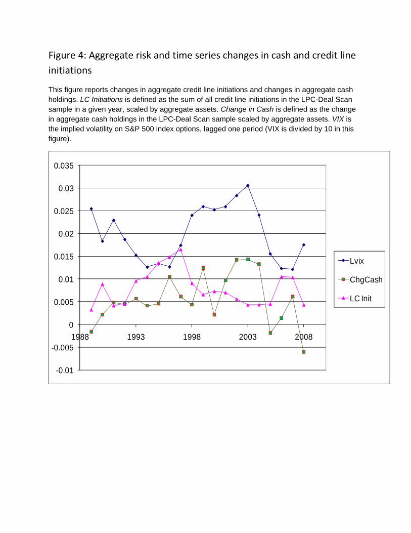
Figure 4: Aggregate risk and time series changes in cash and credit line

initiations

This figure reports changes in aggregate credit line initiations and changes in aggregate cash holdings. LC Initiations is defined as the sum of all credit line initiations in the LPC-Deal Scan sample in a given year, scaled by aggregate assets. Change in Cash is defined as the change in aggregate cash holdings in the LPC-Deal Scan sample scaled by aggregate assets. VIX is the implied volatility on S&P 500 index options, lagged one period (VIX is divided by 10 in this figure).

-0.01

-0.005

0

0.005

0.01

0.015

0.02

0.025

0.03

0.035

1988 1993 1998 2003 2008

Lvix

ChgCash

LC Init

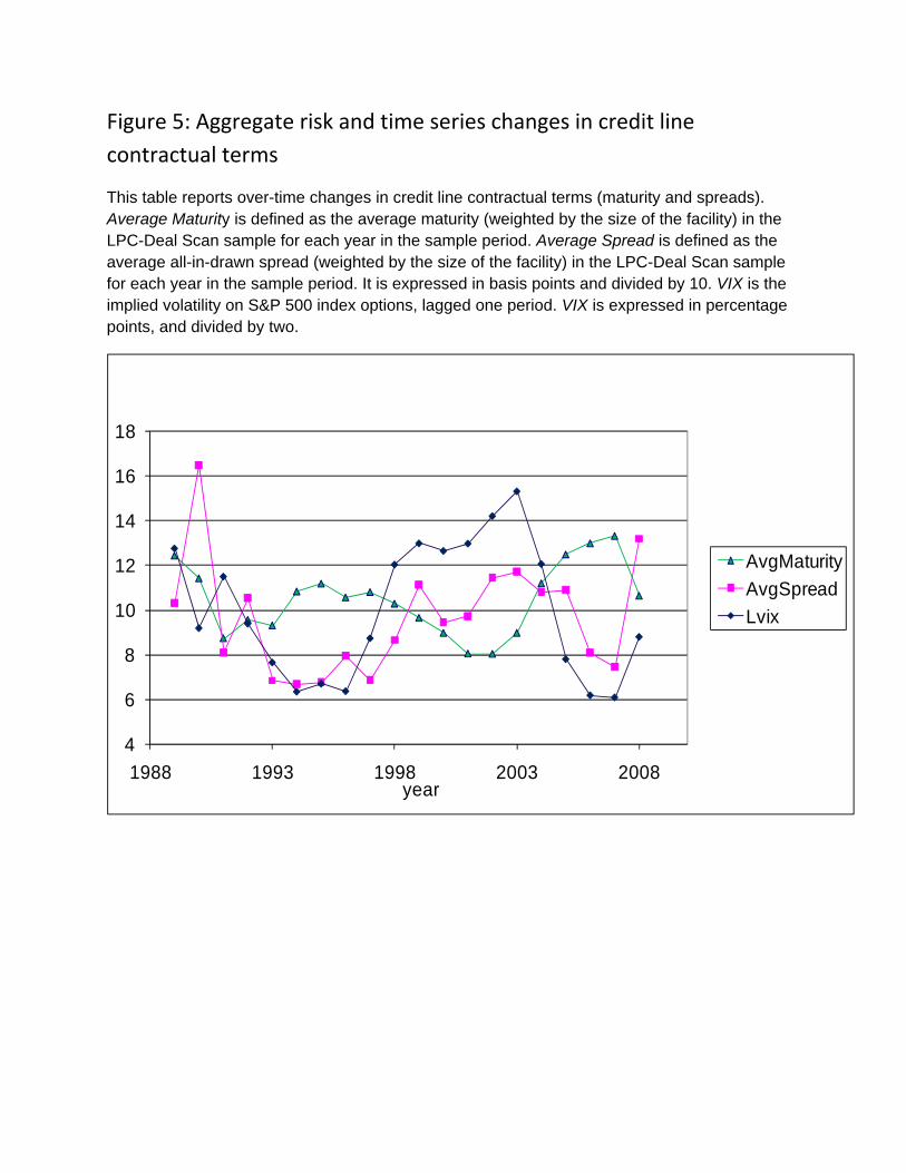
Figure 5: Aggregate risk and time series changes in credit line

contractual terms

This table reports over-time changes in credit line contractual terms (maturity and spreads). Average Maturity is defined as the average maturity (weighted by the size of the facility) in the LPC-Deal Scan sample for each year in the sample period. Average Spread is defined as the average all-in-drawn spread (weighted by the size of the facility) in the LPC-Deal Scan sample for each year in the sample period. It is expressed in basis points and divided by 10. VIX is the implied volatility on S&P 500 index options, lagged one period. VIX is expressed in percentage points, and divided by two.

4

6

8

10

12

14

16

18

1988 1993 1998 2003 2008year

AvgMaturity

AvgSpread

Lvix

Online Appendix:

Aggregate Risk and the Choice between Cash and Lines of Credit*

VIRAL V. ACHARYA, HEITOR ALMEIDA, and, MURILLO CAMPELLO

First draft: September 2009; This draft: June 2012




*Acharya, Viral, Heitor Almeida, and Murillo Campello, 2012, Internet Appendix to “Aggregate Risk and the

Choice between Cash and Lines of Credit,” Journal of Finance [vol #], [pages], http://www.afajof.org/IA/[year].asp.

Please note: Wiley-Blackwell is not responsible for the content or functionality of any supporting information

supplied by the authors. Any queries (other than missing material) should be directed to the authors of the

article."

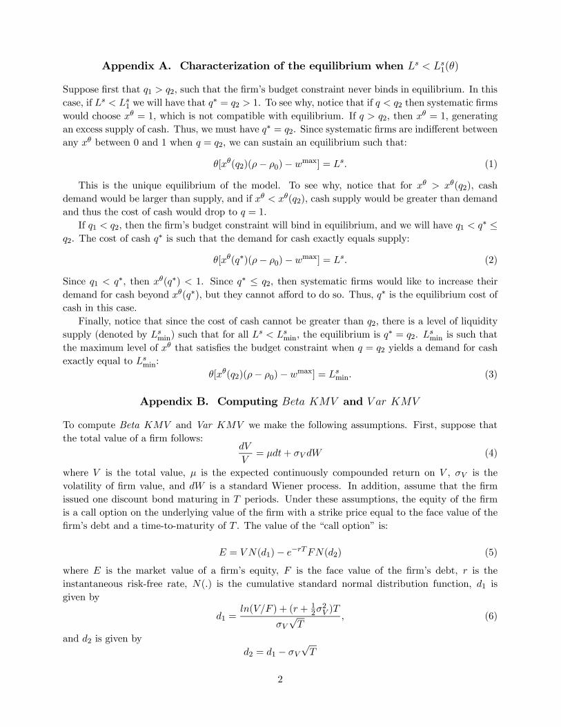
Appendix A. Characterization of the equilibrium when Ls < Ls1(θ)

Suppose first that q1 > q2, such that the firm’s budget constraint never binds in equilibrium. In this

case, if Ls < Ls1 we will have that q∗ = q2 > 1. To see why, notice that if q < q2 then systematic firms

would choose xθ = 1, which is not compatible with equilibrium. If q > q2, then xθ = 1, generating

an excess supply of cash. Thus, we must have q∗ = q2. Since systematic firms are indifferent betweenany xθ between 0 and 1 when q = q2, we can sustain an equilibrium such that:

θ[xθ(q2)(ρ− ρ0)− wmax] = Ls. (1)

This is the unique equilibrium of the model. To see why, notice that for xθ > xθ(q2), cash

demand would be larger than supply, and if xθ < xθ(q2), cash supply would be greater than demand

and thus the cost of cash would drop to q = 1.

If q1 < q2, then the firm’s budget constraint will bind in equilibrium, and we will have q1 < q∗ ≤

q2. The cost of cash q∗ is such that the demand for cash exactly equals supply:

θ[xθ(q∗)(ρ− ρ0)−wmax] = Ls. (2)

Since q1 < q∗, then xθ(q∗) < 1. Since q∗ ≤ q2, then systematic firms would like to increase theirdemand for cash beyond xθ(q∗), but they cannot afford to do so. Thus, q∗ is the equilibrium cost of

cash in this case.

Finally, notice that since the cost of cash cannot be greater than q2, there is a level of liquidity

supply (denoted by Lsmin) such that for all Ls < Lsmin, the equilibrium is q∗ = q2. Lsmin is such that

the maximum level of xθ that satisfies the budget constraint when q = q2 yields a demand for cash

exactly equal to Lsmin:

θ[xθ(q2)(ρ− ρ0)− wmax] = Lsmin. (3)

Appendix B. Computing Beta KMV and V ar KMV

To compute Beta KMV and Var KMV we make the following assumptions. First, suppose that

the total value of a firm follows:dV

V= μdt+ σV dW (4)

where V is the total value, μ is the expected continuously compounded return on V , σV is the

volatility of firm value, and dW is a standard Wiener process. In addition, assume that the firm

issued one discount bond maturing in T periods. Under these assumptions, the equity of the firm

is a call option on the underlying value of the firm with a strike price equal to the face value of the

firm’s debt and a time-to-maturity of T . The value of the “call option” is:

E = V N(d1)− e−rTFN(d2) (5)

where E is the market value of a firm’s equity, F is the face value of the firm’s debt, r is the

instantaneous risk-free rate, N(.) is the cumulative standard normal distribution function, d1 is

given by

d1 =ln(V/F ) + (r + 1

2σ2V )T

σV√T

, (6)

and d2 is given by

d2 = d1 − σV√T

2

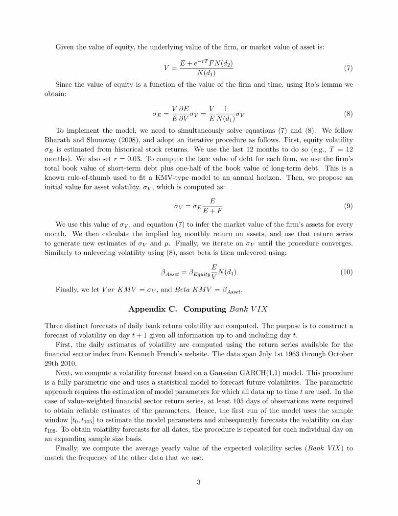
Given the value of equity, the underlying value of the firm, or market value of asset is:

V =E + e−rTFN(d2)

N(d1)(7)

Since the value of equity is a function of the value of the firm and time, using Ito’s lemma we

obtain:

σE =V

E

∂E

∂VσV =

V

E

1

N(d1)σV (8)

To implement the model, we need to simultaneously solve equations (7) and (8). We follow

Bharath and Shumway (2008), and adopt an iterative procedure as follows. First, equity volatility

σE is estimated from historical stock returns. We use the last 12 months to do so (e.g., T = 12

months). We also set r = 0.03. To compute the face value of debt for each firm, we use the firm’s

total book value of short-term debt plus one-half of the book value of long-term debt. This is a

known rule-of-thumb used to fit a KMV-type model to an annual horizon. Then, we propose an

initial value for asset volatility, σV , which is computed as:

σV = σEE

E + F(9)

We use this value of σV , and equation (7) to infer the market value of the firm’s assets for every

month. We then calculate the implied log monthly return on assets, and use that return series

to generate new estimates of σV and μ. Finally, we iterate on σV until the procedure converges.

Similarly to unlevering volatility using (8), asset beta is then unlevered using:

βAsset = βEquityE

VN(d1) (10)

Finally, we let V ar KMV = σV , and Beta KMV = βAsset.

Appendix C. Computing Bank V IX

Three distinct forecasts of daily bank return volatility are computed. The purpose is to construct a

forecast of volatility on day t+ 1 given all information up to and including day t.

First, the daily estimates of volatility are computed using the return series available for the

financial sector index from Kenneth French’s website. The data span July 1st 1963 through October

29th 2010.

Next, we compute a volatility forecast based on a Gaussian GARCH(1,1) model. This procedure

is a fully parametric one and uses a statistical model to forecast future volatilities. The parametric

approach requires the estimation of model parameters for which all data up to time t are used. In the

case of value-weighted financial sector return series, at least 105 days of observations were required

to obtain reliable estimates of the parameters. Hence, the first run of the model uses the sample

window [t0, t105] to estimate the model parameters and subsequently forecasts the volatility on day

t106. To obtain volatility forecasts for all dates, the procedure is repeated for each individual day on

an expanding sample size basis.

Finally, we compute the average yearly value of the expected volatility series (Bank VIX ) to

match the frequency of the other data that we use.

3

Appendix D. Additional robustness tests

In this Section we report a battery of robustness tests that did not fit in the main body of the paper.

In Table AI, we show the results of varying the proxy for aggregate risk exposure using Sufi’s

sample. Panel A shows the results for Total LC-Cash, and Panel B shows results for Unused LC-Cash.

− Table AI about here −

In Table AII, we show the results of partitioning the sample according to different financial

constraints criteria and beta proxies, for the entire range of beta proxies that we employ in the

paper. Each panel from A to G corresponds to a different beta proxy.

− Table AII about here −

In Table AIII, we relate the cost of credit lines to different proxies for beta. Panel A examines

the All-in-Drawn Spread, and Panel B examines the Undrawn Fee.

− Table AIII about here −

In Table AIV, we present results that relate bank-level credit line exposure to bank risk for high

and low VIX months, using different cutoffs to classify months into high and low VIX bins. Panel

A uses a 10% cutoff, and Panel B uses a 25% cutoff.

− Table AIV about here −

In Table AV, we present variations of the tests that link credit line availability to covenant

violations and aggregate risk exposure. In Panel A we use Total LC-to-Assets as a dependent

variable. In Panel B we use Beta KMV instead of VIX as an aggregate risk proxy. In Panel C we

add interactions between VIX and covenant violations and in Panel D we add interactions between

Beta KMV and covenant violations.

− Table AV about here −

4

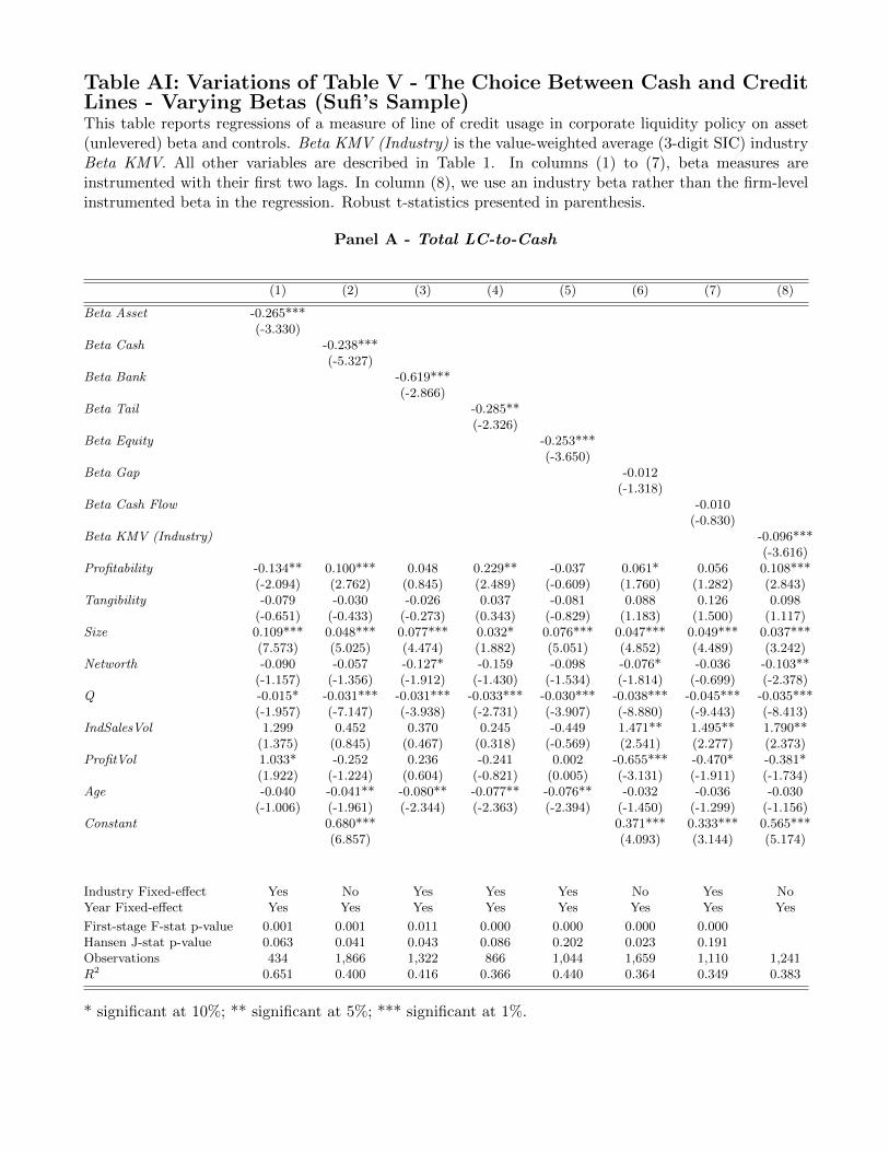
Table AI: Variations of Table V - The Choice Between Cash and CreditLines - Varying Betas (Sufi’s Sample)This table reports regressions of a measure of line of credit usage in corporate liquidity policy on asset(unlevered) beta and controls. Beta KMV (Industry) is the value-weighted average (3-digit SIC) industryBeta KMV. All other variables are described in Table 1. In columns (1) to (7), beta measures areinstrumented with their first two lags. In column (8), we use an industry beta rather than the firm-levelinstrumented beta in the regression. Robust t-statistics presented in parenthesis.

Panel A - Total LC-to-Cash

(1) (2) (3) (4) (5) (6) (7) (8)

Beta Asset -0.265***(-3.330)

Beta Cash -0.238***(-5.327)

Beta Bank -0.619***(-2.866)

Beta Tail -0.285**(-2.326)

Beta Equity -0.253***(-3.650)

Beta Gap -0.012(-1.318)

Beta Cash Flow -0.010(-0.830)


Profitability -0.134** 0.100*** 0.048 0.229** -0.037 0.061* 0.056 0.108***(-2.094) (2.762) (0.845) (2.489) (-0.609) (1.760) (1.282) (2.843)

Tangibility -0.079 -0.030 -0.026 0.037 -0.081 0.088 0.126 0.098(-0.651) (-0.433) (-0.273) (0.343) (-0.829) (1.183) (1.500) (1.117)

Size 0.109*** 0.048*** 0.077*** 0.032* 0.076*** 0.047*** 0.049*** 0.037***(7.573) (5.025) (4.474) (1.882) (5.051) (4.852) (4.489) (3.242)

Networth -0.090 -0.057 -0.127* -0.159 -0.098 -0.076* -0.036 -0.103**(-1.157) (-1.356) (-1.912) (-1.430) (-1.534) (-1.814) (-0.699) (-2.378)

Q -0.015* -0.031*** -0.031*** -0.033*** -0.030*** -0.038*** -0.045*** -0.035***(-1.957) (-7.147) (-3.938) (-2.731) (-3.907) (-8.880) (-9.443) (-8.413)

IndSalesVol 1.299 0.452 0.370 0.245 -0.449 1.471** 1.495** 1.790**(1.375) (0.845) (0.467) (0.318) (-0.569) (2.541) (2.277) (2.373)

ProfitVol 1.033* -0.252 0.236 -0.241 0.002 -0.655*** -0.470* -0.381*(1.922) (-1.224) (0.604) (-0.821) (0.005) (-3.131) (-1.911) (-1.734)

Age -0.040 -0.041** -0.080** -0.077** -0.076** -0.032 -0.036 -0.030(-1.006) (-1.961) (-2.344) (-2.363) (-2.394) (-1.450) (-1.299) (-1.156)

Constant 0.680*** 0.371*** 0.333*** 0.565***(6.857) (4.093) (3.144) (5.174)


First-stage F-stat p-value 0.001 0.001 0.011 0.000 0.000 0.000 0.000Hansen J-stat p-value 0.063 0.041 0.043 0.086 0.202 0.023 0.191Observations 434 1,866 1,322 866 1,044 1,659 1,110 1,241R2 0.651 0.400 0.416 0.366 0.440 0.364 0.349 0.383


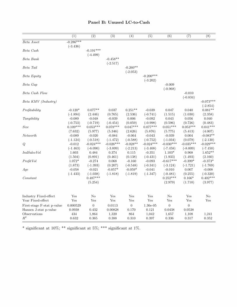
Panel B: Unused LC-to-Cash

(1) (2) (3) (4) (5) (6) (7) (8)

Beta Asset -0.286***(-3.436)

Beta Cash -0.191***(-4.499)

Beta Bank -0.458**(-2.517)

Beta Tail -0.260**(-2.053)

Beta Equity -0.200***(-3.202)

Beta Gap -0.009(-0.968)



Profitability -0.120* 0.077** 0.037 0.251** -0.039 0.047 0.040 0.081**(-1.894) (2.446) (0.765) (2.536) (-0.741) (1.515) (1.030) (2.358)

Tangibility -0.089 -0.048 -0.039 0.006 -0.092 0.043 0.056 0.040(-0.753) (-0.719) (-0.454) (0.059) (-0.998) (0.596) (0.726) (0.483)

Size 0.109*** 0.053*** 0.078*** 0.047*** 0.077*** 0.051*** 0.053*** 0.041***(7.632) (5.977) (5.346) (2.626) (5.876) (5.775) (5.413) (4.007)

Networth -0.089 -0.020 -0.084 -0.064 -0.043 -0.039 0.004 -0.083**(-1.124) (-0.518) (-1.472) (-0.588) (-0.752) (-1.034) (0.079) (-2.130)

Q -0.012 -0.024*** -0.026*** -0.028** -0.024*** -0.030*** -0.035*** -0.029***(-1.463) (-6.090) (-3.899) (-2.213) (-3.408) (-7.458) (-8.009) (-7.450)

IndSalesVol 1.603 0.484 0.374 0.115 -0.351 1.103* 0.968 1.652**(1.504) (0.891) (0.461) (0.138) (-0.431) (1.933) (1.493) (2.160)

ProfitVol 1.072* -0.274 0.068 -0.160 -0.093 -0.617*** -0.399* -0.373*(1.873) (-1.393) (0.207) (-0.548) (-0.341) (-3.124) (-1.721) (-1.769)

Age -0.058 -0.021 -0.057* -0.059* -0.041 -0.010 0.007 -0.008(-1.433) (-1.038) (-1.818) (-1.819) (-1.347) (-0.481) (0.255) (-0.320)

Constant 0.487*** 0.252*** 0.166* 0.402***(5.254) (2.979) (1.710) (3.977)


First-stage F-stat p-value 0.000529 0 0.0113 0 1.36e-05 0 0Hansen J-stat p-value 0.0938 0.432 0.00828 0.170 0.121 0.0438 0.0538Observations 434 1,864 1,320 864 1,042 1,657 1,108 1,241R2 0.632 0.365 0.388 0.310 0.397 0.336 0.317 0.352


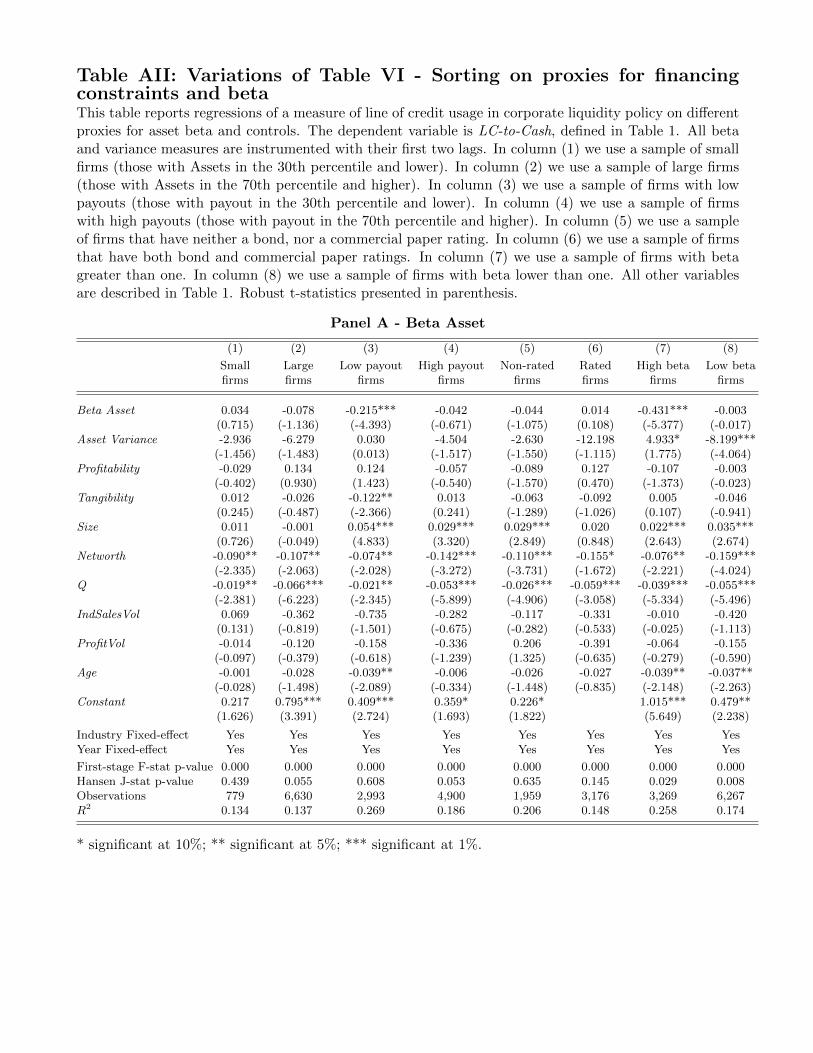
Table AII: Variations of Table VI - Sorting on proxies for financingconstraints and betaThis table reports regressions of a measure of line of credit usage in corporate liquidity policy on differentproxies for asset beta and controls. The dependent variable is LC-to-Cash, defined in Table 1. All betaand variance measures are instrumented with their first two lags. In column (1) we use a sample of smallfirms (those with Assets in the 30th percentile and lower). In column (2) we use a sample of large firms(those with Assets in the 70th percentile and higher). In column (3) we use a sample of firms with lowpayouts (those with payout in the 30th percentile and lower). In column (4) we use a sample of firmswith high payouts (those with payout in the 70th percentile and higher). In column (5) we use a sampleof firms that have neither a bond, nor a commercial paper rating. In column (6) we use a sample of firmsthat have both bond and commercial paper ratings. In column (7) we use a sample of firms with betagreater than one. In column (8) we use a sample of firms with beta lower than one. All other variablesare described in Table 1. Robust t-statistics presented in parenthesis.

Panel A - Beta Asset

(1) (2) (3) (4) (5) (6) (7) (8)

Small Large Low payout High payout Non-rated Rated High beta Low betafirms firms firms firms firms firms firms firms

Beta Asset 0.034 -0.078 -0.215*** -0.042 -0.044 0.014 -0.431*** -0.003(0.715) (-1.136) (-4.393) (-0.671) (-1.075) (0.108) (-5.377) (-0.017)

Asset Variance -2.936 -6.279 0.030 -4.504 -2.630 -12.198 4.933* -8.199***(-1.456) (-1.483) (0.013) (-1.517) (-1.550) (-1.115) (1.775) (-4.064)

Profitability -0.029 0.134 0.124 -0.057 -0.089 0.127 -0.107 -0.003(-0.402) (0.930) (1.423) (-0.540) (-1.570) (0.470) (-1.373) (-0.023)

Tangibility 0.012 -0.026 -0.122** 0.013 -0.063 -0.092 0.005 -0.046(0.245) (-0.487) (-2.366) (0.241) (-1.289) (-1.026) (0.107) (-0.941)

Size 0.011 -0.001 0.054*** 0.029*** 0.029*** 0.020 0.022*** 0.035***(0.726) (-0.049) (4.833) (3.320) (2.849) (0.848) (2.643) (2.674)

Networth -0.090** -0.107** -0.074** -0.142*** -0.110*** -0.155* -0.076** -0.159***(-2.335) (-2.063) (-2.028) (-3.272) (-3.731) (-1.672) (-2.221) (-4.024)

Q -0.019** -0.066*** -0.021** -0.053*** -0.026*** -0.059*** -0.039*** -0.055***(-2.381) (-6.223) (-2.345) (-5.899) (-4.906) (-3.058) (-5.334) (-5.496)

IndSalesVol 0.069 -0.362 -0.735 -0.282 -0.117 -0.331 -0.010 -0.420(0.131) (-0.819) (-1.501) (-0.675) (-0.282) (-0.533) (-0.025) (-1.113)

ProfitVol -0.014 -0.120 -0.158 -0.336 0.206 -0.391 -0.064 -0.155(-0.097) (-0.379) (-0.618) (-1.239) (1.325) (-0.635) (-0.279) (-0.590)

Age -0.001 -0.028 -0.039** -0.006 -0.026 -0.027 -0.039** -0.037**(-0.028) (-1.498) (-2.089) (-0.334) (-1.448) (-0.835) (-2.148) (-2.263)

Constant 0.217 0.795*** 0.409*** 0.359* 0.226* 1.015*** 0.479**(1.626) (3.391) (2.724) (1.693) (1.822) (5.649) (2.238)


First-stage F-stat p-value 0.000 0.000 0.000 0.000 0.000 0.000 0.000 0.000Hansen J-stat p-value 0.439 0.055 0.608 0.053 0.635 0.145 0.029 0.008Observations 779 6,630 2,993 4,900 1,959 3,176 3,269 6,267R2 0.134 0.137 0.269 0.186 0.206 0.148 0.258 0.174


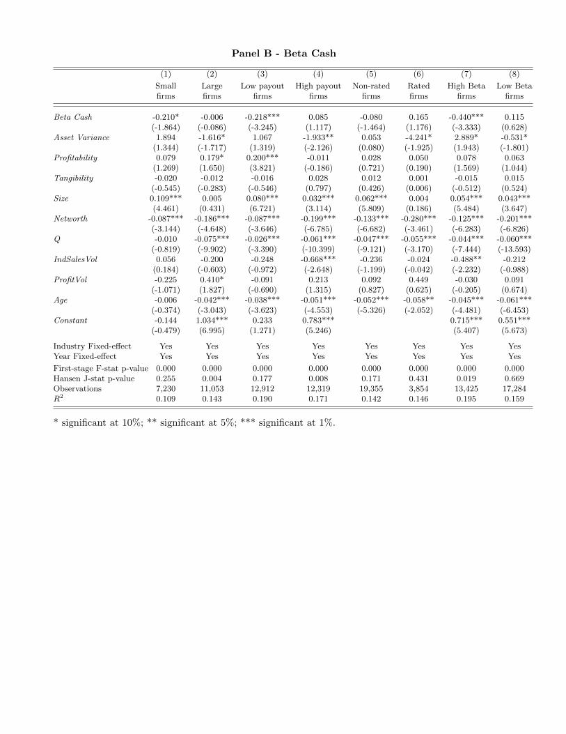
Panel B - Beta Cash

(1) (2) (3) (4) (5) (6) (7) (8)


Beta Cash -0.210* -0.006 -0.218*** 0.085 -0.080 0.165 -0.440*** 0.115(-1.864) (-0.086) (-3.245) (1.117) (-1.464) (1.176) (-3.333) (0.628)

Asset Variance 1.894 -1.616* 1.067 -1.933** 0.053 -4.241* 2.889* -0.531*(1.344) (-1.717) (1.319) (-2.126) (0.080) (-1.925) (1.943) (-1.801)

Profitability 0.079 0.179* 0.200*** -0.011 0.028 0.050 0.078 0.063(1.269) (1.650) (3.821) (-0.186) (0.721) (0.190) (1.569) (1.044)

Tangibility -0.020 -0.012 -0.016 0.028 0.012 0.001 -0.015 0.015(-0.545) (-0.283) (-0.546) (0.797) (0.426) (0.006) (-0.512) (0.524)

Size 0.109*** 0.005 0.080*** 0.032*** 0.062*** 0.004 0.054*** 0.043***(4.461) (0.431) (6.721) (3.114) (5.809) (0.186) (5.484) (3.647)

Networth -0.087*** -0.186*** -0.087*** -0.199*** -0.133*** -0.280*** -0.125*** -0.201***(-3.144) (-4.648) (-3.646) (-6.785) (-6.682) (-3.461) (-6.283) (-6.826)

Q -0.010 -0.075*** -0.026*** -0.061*** -0.047*** -0.055*** -0.044*** -0.060***(-0.819) (-9.902) (-3.390) (-10.399) (-9.121) (-3.170) (-7.444) (-13.593)

IndSalesVol 0.056 -0.200 -0.248 -0.668*** -0.236 -0.024 -0.488** -0.212(0.184) (-0.603) (-0.972) (-2.648) (-1.199) (-0.042) (-2.232) (-0.988)

ProfitVol -0.225 0.410* -0.091 0.213 0.092 0.449 -0.030 0.091(-1.071) (1.827) (-0.690) (1.315) (0.827) (0.625) (-0.205) (0.674)

Age -0.006 -0.042*** -0.038*** -0.051*** -0.052*** -0.058** -0.045*** -0.061***(-0.374) (-3.043) (-3.623) (-4.553) (-5.326) (-2.052) (-4.481) (-6.453)

Constant -0.144 1.034*** 0.233 0.783*** 0.715*** 0.551***(-0.479) (6.995) (1.271) (5.246) (5.407) (5.673)


First-stage F-stat p-value 0.000 0.000 0.000 0.000 0.000 0.000 0.000 0.000Hansen J-stat p-value 0.255 0.004 0.177 0.008 0.171 0.431 0.019 0.669Observations 7,230 11,053 12,912 12,319 19,355 3,854 13,425 17,284R2 0.109 0.143 0.190 0.171 0.142 0.146 0.195 0.159


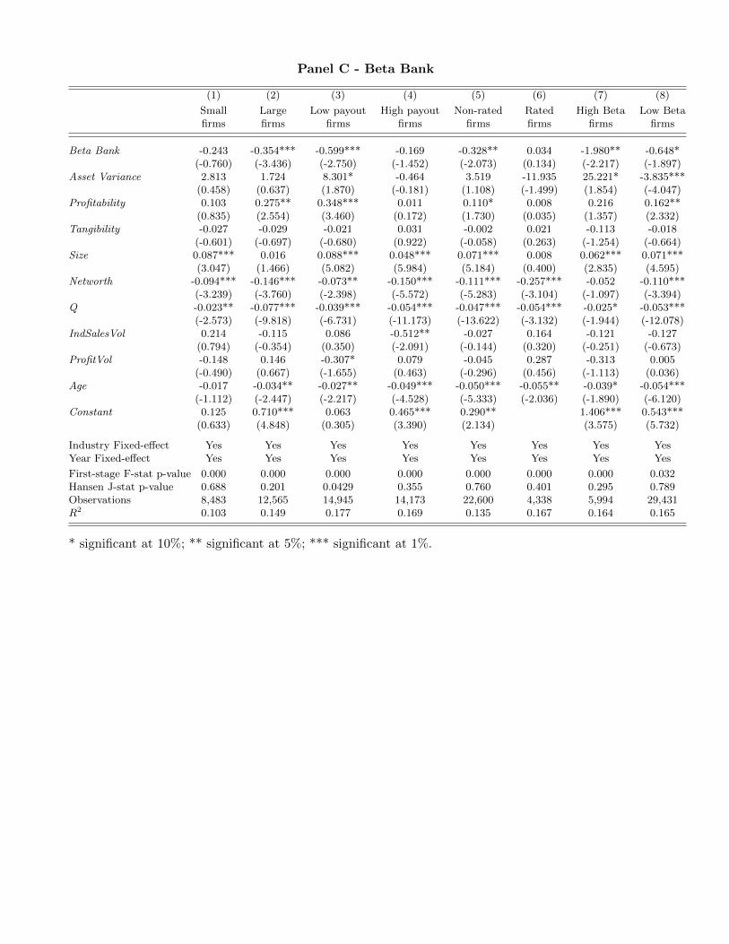
Panel C - Beta Bank

(1) (2) (3) (4) (5) (6) (7) (8)


Beta Bank -0.243 -0.354*** -0.599*** -0.169 -0.328** 0.034 -1.980** -0.648*(-0.760) (-3.436) (-2.750) (-1.452) (-2.073) (0.134) (-2.217) (-1.897)

Asset Variance 2.813 1.724 8.301* -0.464 3.519 -11.935 25.221* -3.835***(0.458) (0.637) (1.870) (-0.181) (1.108) (-1.499) (1.854) (-4.047)

Profitability 0.103 0.275** 0.348*** 0.011 0.110* 0.008 0.216 0.162**(0.835) (2.554) (3.460) (0.172) (1.730) (0.035) (1.357) (2.332)

Tangibility -0.027 -0.029 -0.021 0.031 -0.002 0.021 -0.113 -0.018(-0.601) (-0.697) (-0.680) (0.922) (-0.058) (0.263) (-1.254) (-0.664)

Size 0.087*** 0.016 0.088*** 0.048*** 0.071*** 0.008 0.062*** 0.071***(3.047) (1.466) (5.082) (5.984) (5.184) (0.400) (2.835) (4.595)

Networth -0.094*** -0.146*** -0.073** -0.150*** -0.111*** -0.257*** -0.052 -0.110***(-3.239) (-3.760) (-2.398) (-5.572) (-5.283) (-3.104) (-1.097) (-3.394)

Q -0.023** -0.077*** -0.039*** -0.054*** -0.047*** -0.054*** -0.025* -0.053***(-2.573) (-9.818) (-6.731) (-11.173) (-13.622) (-3.132) (-1.944) (-12.078)

IndSalesVol 0.214 -0.115 0.086 -0.512** -0.027 0.164 -0.121 -0.127(0.794) (-0.354) (0.350) (-2.091) (-0.144) (0.320) (-0.251) (-0.673)

ProfitVol -0.148 0.146 -0.307* 0.079 -0.045 0.287 -0.313 0.005(-0.490) (0.667) (-1.655) (0.463) (-0.296) (0.456) (-1.113) (0.036)

Age -0.017 -0.034** -0.027** -0.049*** -0.050*** -0.055** -0.039* -0.054***(-1.112) (-2.447) (-2.217) (-4.528) (-5.333) (-2.036) (-1.890) (-6.120)

Constant 0.125 0.710*** 0.063 0.465*** 0.290** 1.406*** 0.543***(0.633) (4.848) (0.305) (3.390) (2.134) (3.575) (5.732)


First-stage F-stat p-value 0.000 0.000 0.000 0.000 0.000 0.000 0.000 0.032Hansen J-stat p-value 0.688 0.201 0.0429 0.355 0.760 0.401 0.295 0.789Observations 8,483 12,565 14,945 14,173 22,600 4,338 5,994 29,431R2 0.103 0.149 0.177 0.169 0.135 0.167 0.164 0.165


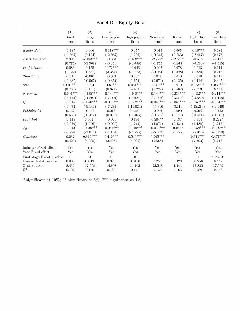
Panel D - Equity Beta

(1) (2) (3) (4) (5) (6) (7) (8)


Equity Beta -0.137 0.006 -0.118*** 0.057 -0.013 0.065 -0.167** 0.082(-1.365) (0.124) (-2.665) (1.226) (-0.343) (0.783) (-2.467) (0.678)

Asset Variance 2.995 -7.103*** -0.088 -6.188*** -2.772* -12.553* -0.575 -2.417(0.775) (-2.969) (-0.051) (-3.049) (-1.752) (-1.917) (-0.288) (-1.515)

Profitability 0.083 0.155 0.172*** -0.046 -0.002 0.078 0.013 0.014(1.122) (1.581) (3.384) (-0.772) (-0.054) (0.328) (0.330) (0.218)

Tangibility -0.011 -0.003 -0.009 0.037 0.017 0.010 0.010 0.012(-0.337) (-0.067) (-0.355) (1.155) (0.670) (0.125) (0.414) (0.445)

Size 0.097*** 0.004 0.067*** 0.031*** 0.047*** 0.010 0.033*** 0.039***(3.753) (0.431) (6.674) (4.169) (5.224) (0.507) (7.673) (3.651)

Networth -0.094*** -0.185*** -0.136*** -0.168*** -0.134*** -0.239*** -0.182*** -0.214***(-4.175) (-4.891) (-7.009) (-6.621) (-7.926) (-3.205) (-5.580) (-4.415)

Q -0.015 -0.066*** -0.036*** -0.052*** -0.048*** -0.053*** -0.057*** -0.054***(-1.372) (-9.140) (-7.234) (-11.024) (-13.896) (-3.119) (-15.210) (-9.046)

IndSalesVol 0.162 -0.149 0.013 -0.588** -0.056 0.090 -0.092 -0.222(0.565) (-0.472) (0.056) (-2.466) (-0.306) (0.171) (-0.491) (-1.081)

ProfitVol -0.115 0.362* -0.001 0.190 0.204** 0.137 0.154 0.227*(-0.570) (1.696) (-0.007) (1.243) (2.071) (0.224) (1.488) (1.717)

Age -0.013 -0.039*** -0.041*** -0.049*** -0.056*** -0.046* -0.058*** -0.059***(-0.776) (-3.014) (-4.154) (-4.555) (-6.332) (-1.727) (-5.956) (-6.270)

Constant 0.082 0.815*** 0.410*** 0.546*** 0.505*** 0.911*** 0.477***(0.429) (5.835) (3.408) (4.396) (5.568) (7.393) (5.216)


First-stage F-stat p-value 0 0 0 0 0 0 0 4.92e-06Hansen J-stat p-value 0.908 0.00131 0.323 0.0156 0.256 0.323 0.0256 0.348Observations 8,436 12,578 14,908 14,162 22,548 4,344 17,833 17,539R2 0.102 0.150 0.180 0.171 0.136 0.165 0.188 0.156


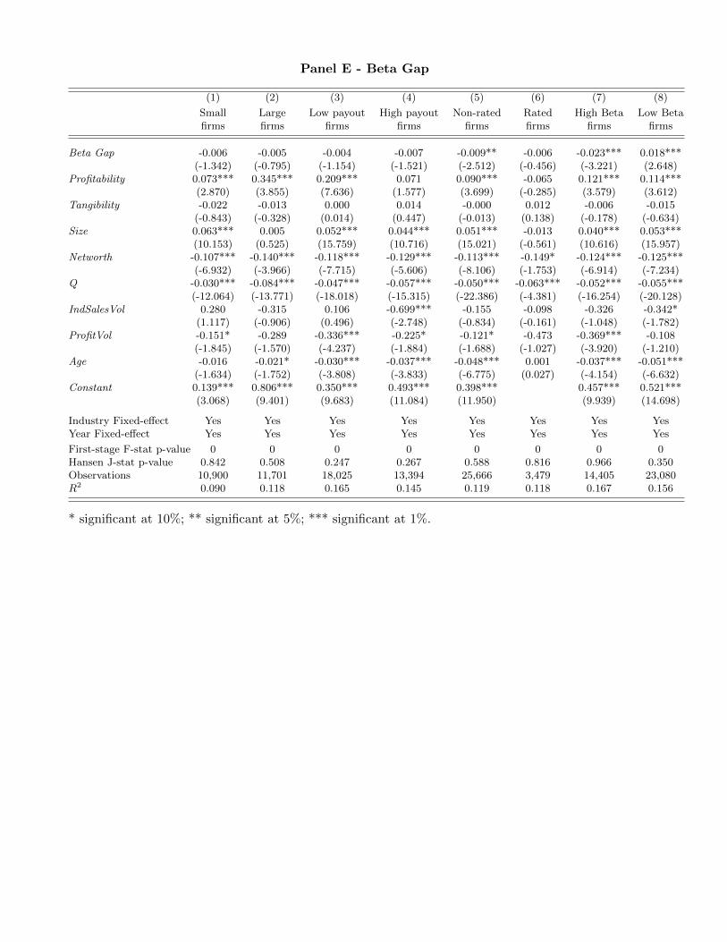
Panel E - Beta Gap

(1) (2) (3) (4) (5) (6) (7) (8)


Beta Gap -0.006 -0.005 -0.004 -0.007 -0.009** -0.006 -0.023*** 0.018***(-1.342) (-0.795) (-1.154) (-1.521) (-2.512) (-0.456) (-3.221) (2.648)

Profitability 0.073*** 0.345*** 0.209*** 0.071 0.090*** -0.065 0.121*** 0.114***(2.870) (3.855) (7.636) (1.577) (3.699) (-0.285) (3.579) (3.612)

Tangibility -0.022 -0.013 0.000 0.014 -0.000 0.012 -0.006 -0.015(-0.843) (-0.328) (0.014) (0.447) (-0.013) (0.138) (-0.178) (-0.634)

Size 0.063*** 0.005 0.052*** 0.044*** 0.051*** -0.013 0.040*** 0.053***(10.153) (0.525) (15.759) (10.716) (15.021) (-0.561) (10.616) (15.957)

Networth -0.107*** -0.140*** -0.118*** -0.129*** -0.113*** -0.149* -0.124*** -0.125***(-6.932) (-3.966) (-7.715) (-5.606) (-8.106) (-1.753) (-6.914) (-7.234)

Q -0.030*** -0.084*** -0.047*** -0.057*** -0.050*** -0.063*** -0.052*** -0.055***(-12.064) (-13.771) (-18.018) (-15.315) (-22.386) (-4.381) (-16.254) (-20.128)

IndSalesVol 0.280 -0.315 0.106 -0.699*** -0.155 -0.098 -0.326 -0.342*(1.117) (-0.906) (0.496) (-2.748) (-0.834) (-0.161) (-1.048) (-1.782)

ProfitVol -0.151* -0.289 -0.336*** -0.225* -0.121* -0.473 -0.369*** -0.108(-1.845) (-1.570) (-4.237) (-1.884) (-1.688) (-1.027) (-3.920) (-1.210)

Age -0.016 -0.021* -0.030*** -0.037*** -0.048*** 0.001 -0.037*** -0.051***(-1.634) (-1.752) (-3.808) (-3.833) (-6.775) (0.027) (-4.154) (-6.632)

Constant 0.139*** 0.806*** 0.350*** 0.493*** 0.398*** 0.457*** 0.521***(3.068) (9.401) (9.683) (11.084) (11.950) (9.939) (14.698)


First-stage F-stat p-value 0 0 0 0 0 0 0 0Hansen J-stat p-value 0.842 0.508 0.247 0.267 0.588 0.816 0.966 0.350Observations 10,900 11,701 18,025 13,394 25,666 3,479 14,405 23,080R2 0.090 0.118 0.165 0.145 0.119 0.118 0.167 0.156


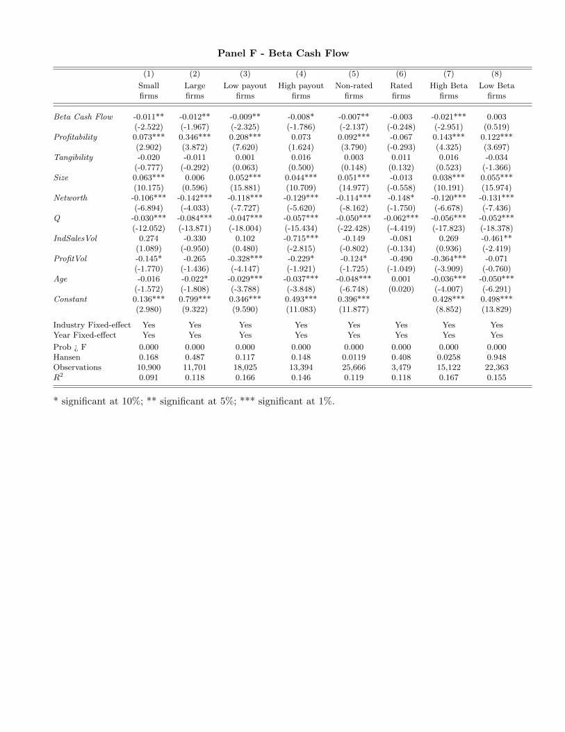
Panel F - Beta Cash Flow

(1) (2) (3) (4) (5) (6) (7) (8)


Beta Cash Flow -0.011** -0.012** -0.009** -0.008* -0.007** -0.003 -0.021*** 0.003(-2.522) (-1.967) (-2.325) (-1.786) (-2.137) (-0.248) (-2.951) (0.519)

Profitability 0.073*** 0.346*** 0.208*** 0.073 0.092*** -0.067 0.143*** 0.122***(2.902) (3.872) (7.620) (1.624) (3.790) (-0.293) (4.325) (3.697)

Tangibility -0.020 -0.011 0.001 0.016 0.003 0.011 0.016 -0.034(-0.777) (-0.292) (0.063) (0.500) (0.148) (0.132) (0.523) (-1.366)

Size 0.063*** 0.006 0.052*** 0.044*** 0.051*** -0.013 0.038*** 0.055***(10.175) (0.596) (15.881) (10.709) (14.977) (-0.558) (10.191) (15.974)

Networth -0.106*** -0.142*** -0.118*** -0.129*** -0.114*** -0.148* -0.120*** -0.131***(-6.894) (-4.033) (-7.727) (-5.620) (-8.162) (-1.750) (-6.678) (-7.436)

Q -0.030*** -0.084*** -0.047*** -0.057*** -0.050*** -0.062*** -0.056*** -0.052***(-12.052) (-13.871) (-18.004) (-15.434) (-22.428) (-4.419) (-17.823) (-18.378)

IndSalesVol 0.274 -0.330 0.102 -0.715*** -0.149 -0.081 0.269 -0.461**(1.089) (-0.950) (0.480) (-2.815) (-0.802) (-0.134) (0.936) (-2.419)

ProfitVol -0.145* -0.265 -0.328*** -0.229* -0.124* -0.490 -0.364*** -0.071(-1.770) (-1.436) (-4.147) (-1.921) (-1.725) (-1.049) (-3.909) (-0.760)

Age -0.016 -0.022* -0.029*** -0.037*** -0.048*** 0.001 -0.036*** -0.050***(-1.572) (-1.808) (-3.788) (-3.848) (-6.748) (0.020) (-4.007) (-6.291)

Constant 0.136*** 0.799*** 0.346*** 0.493*** 0.396*** 0.428*** 0.498***(2.980) (9.322) (9.590) (11.083) (11.877) (8.852) (13.829)


Prob ¿ F 0.000 0.000 0.000 0.000 0.000 0.000 0.000 0.000Hansen 0.168 0.487 0.117 0.148 0.0119 0.408 0.0258 0.948Observations 10,900 11,701 18,025 13,394 25,666 3,479 15,122 22,363R2 0.091 0.118 0.166 0.146 0.119 0.118 0.167 0.155


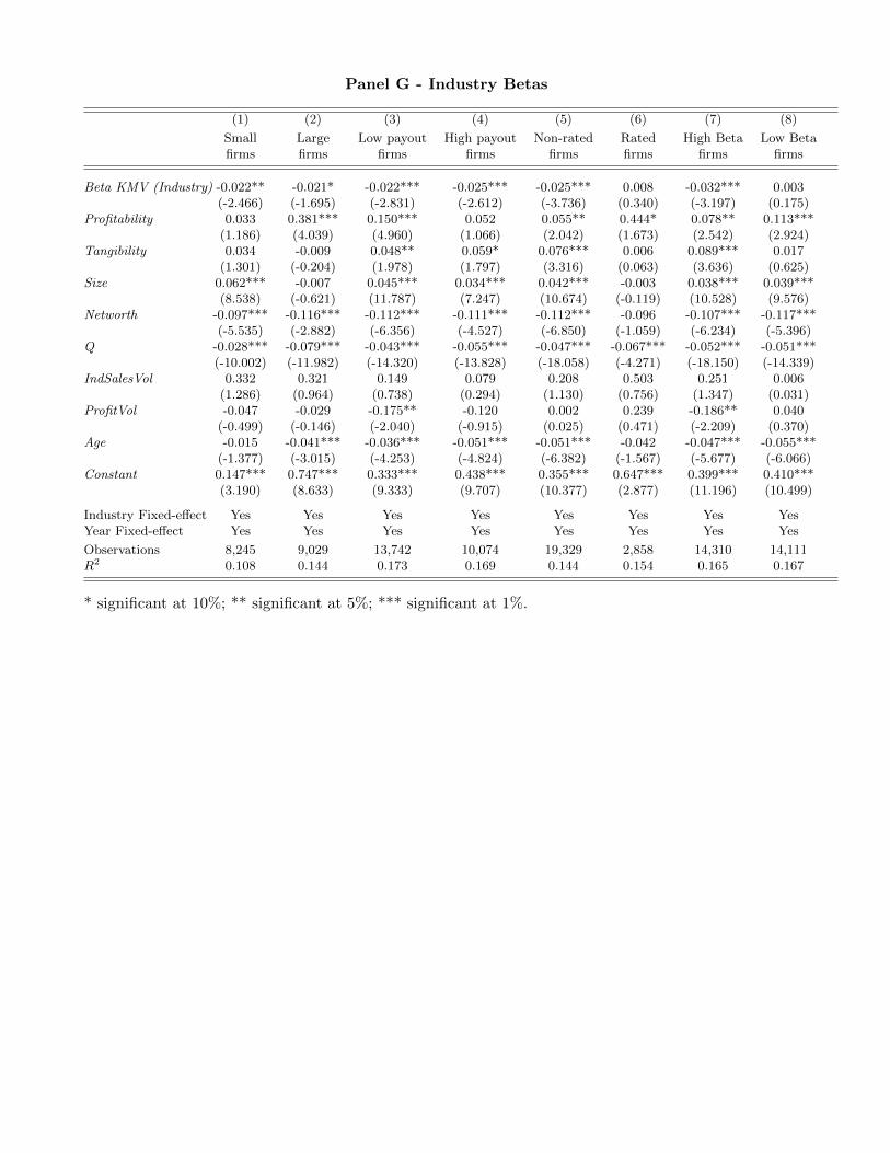
Panel G - Industry Betas

(1) (2) (3) (4) (5) (6) (7) (8)


Beta KMV (Industry) -0.022** -0.021* -0.022*** -0.025*** -0.025*** 0.008 -0.032*** 0.003(-2.466) (-1.695) (-2.831) (-2.612) (-3.736) (0.340) (-3.197) (0.175)

Profitability 0.033 0.381*** 0.150*** 0.052 0.055** 0.444* 0.078** 0.113***(1.186) (4.039) (4.960) (1.066) (2.042) (1.673) (2.542) (2.924)

Tangibility 0.034 -0.009 0.048** 0.059* 0.076*** 0.006 0.089*** 0.017(1.301) (-0.204) (1.978) (1.797) (3.316) (0.063) (3.636) (0.625)

Size 0.062*** -0.007 0.045*** 0.034*** 0.042*** -0.003 0.038*** 0.039***(8.538) (-0.621) (11.787) (7.247) (10.674) (-0.119) (10.528) (9.576)

Networth -0.097*** -0.116*** -0.112*** -0.111*** -0.112*** -0.096 -0.107*** -0.117***(-5.535) (-2.882) (-6.356) (-4.527) (-6.850) (-1.059) (-6.234) (-5.396)

Q -0.028*** -0.079*** -0.043*** -0.055*** -0.047*** -0.067*** -0.052*** -0.051***(-10.002) (-11.982) (-14.320) (-13.828) (-18.058) (-4.271) (-18.150) (-14.339)

IndSalesVol 0.332 0.321 0.149 0.079 0.208 0.503 0.251 0.006(1.286) (0.964) (0.738) (0.294) (1.130) (0.756) (1.347) (0.031)

ProfitVol -0.047 -0.029 -0.175** -0.120 0.002 0.239 -0.186** 0.040(-0.499) (-0.146) (-2.040) (-0.915) (0.025) (0.471) (-2.209) (0.370)

Age -0.015 -0.041*** -0.036*** -0.051*** -0.051*** -0.042 -0.047*** -0.055***(-1.377) (-3.015) (-4.253) (-4.824) (-6.382) (-1.567) (-5.677) (-6.066)

Constant 0.147*** 0.747*** 0.333*** 0.438*** 0.355*** 0.647*** 0.399*** 0.410***(3.190) (8.633) (9.333) (9.707) (10.377) (2.877) (11.196) (10.499)


Observations 8,245 9,029 13,742 10,074 19,329 2,858 14,310 14,111R2 0.108 0.144 0.173 0.169 0.144 0.154 0.165 0.167


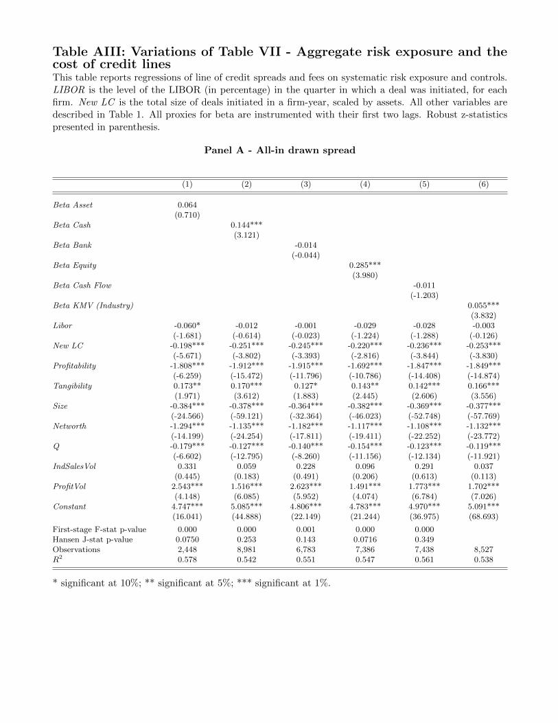
Table AIII: Variations of Table VII - Aggregate risk exposure and thecost of credit linesThis table reports regressions of line of credit spreads and fees on systematic risk exposure and controls.LIBOR is the level of the LIBOR (in percentage) in the quarter in which a deal was initiated, for eachfirm. New LC is the total size of deals initiated in a firm-year, scaled by assets. All other variables aredescribed in Table 1. All proxies for beta are instrumented with their first two lags. Robust z-statisticspresented in parenthesis.

Panel A - All-in drawn spread

(1) (2) (3) (4) (5) (6)

Beta Asset 0.064(0.710)

Beta Cash 0.144***(3.121)

Beta Bank -0.014(-0.044)

Beta Equity 0.285***(3.980)


Beta KMV (Industry) 0.055***(3.832)

Libor -0.060* -0.012 -0.001 -0.029 -0.028 -0.003(-1.681) (-0.614) (-0.023) (-1.224) (-1.288) (-0.126)

New LC -0.198*** -0.251*** -0.245*** -0.220*** -0.236*** -0.253***(-5.671) (-3.802) (-3.393) (-2.816) (-3.844) (-3.830)

Profitability -1.808*** -1.912*** -1.915*** -1.692*** -1.847*** -1.849***(-6.259) (-15.472) (-11.796) (-10.786) (-14.408) (-14.874)

Tangibility 0.173** 0.170*** 0.127* 0.143** 0.142*** 0.166***(1.971) (3.612) (1.883) (2.445) (2.606) (3.556)

Size -0.384*** -0.378*** -0.364*** -0.382*** -0.369*** -0.377***(-24.566) (-59.121) (-32.364) (-46.023) (-52.748) (-57.769)

Networth -1.294*** -1.135*** -1.182*** -1.117*** -1.108*** -1.132***(-14.199) (-24.254) (-17.811) (-19.411) (-22.252) (-23.772)

Q -0.179*** -0.127*** -0.140*** -0.154*** -0.123*** -0.119***(-6.602) (-12.795) (-8.260) (-11.156) (-12.134) (-11.921)

IndSalesVol 0.331 0.059 0.228 0.096 0.291 0.037(0.445) (0.183) (0.491) (0.206) (0.613) (0.113)

ProfitVol 2.543*** 1.516*** 2.623*** 1.491*** 1.773*** 1.702***(4.148) (6.085) (5.952) (4.074) (6.784) (7.026)

Constant 4.747*** 5.085*** 4.806*** 4.783*** 4.970*** 5.091***(16.041) (44.888) (22.149) (21.244) (36.975) (68.693)

First-stage F-stat p-value 0.000 0.000 0.001 0.000 0.000Hansen J-stat p-value 0.0750 0.253 0.143 0.0716 0.349Observations 2,448 8,981 6,783 7,386 7,438 8,527R2 0.578 0.542 0.551 0.547 0.561 0.538


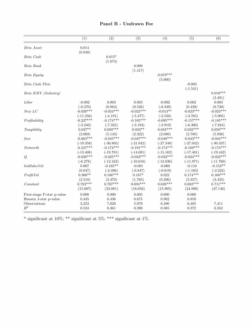
Panel B - Undrawn Fee

(1) (2) (3) (4) (5) (6)

Beta Asset 0.014(0.848)

Beta Cash 0.015*(1.674)

Beta Bank 0.099(1.417)

Beta Equity 0.079***(5.060)


Beta KMV (Industry) 0.010***(3.491)

Libor -0.002 0.003 0.003 -0.002 0.002 0.003(-0.270) (0.884) (0.526) (-0.349) (0.439) (0.730)

New LC -0.026*** -0.024*** -0.022*** -0.013** -0.023*** -0.023***(-11.256) (-4.191) (-5.477) (-2.550) (-3.765) (-5.905)

Profitability -0.227*** -0.174*** -0.105*** -0.095*** -0.157*** -0.185***(-3.240) (-7.325) (-3.194) (-2.919) (-6.300) (-7.824)

Tangibility 0.037** 0.050*** 0.033** 0.034*** 0.032*** 0.058***(2.069) (5.143) (2.322) (2.680) (2.788) (5.936)

Size -0.063*** -0.045*** -0.047*** -0.048*** -0.043*** -0.044***(-19.358) (-30.805) (-21.042) (-27.348) (-27.042) (-30.337)

Networth -0.247*** -0.174*** -0.191*** -0.174*** -0.169*** -0.174***(-13.408) (-19.701) (-14.691) (-15.162) (-17.401) (-19.442)

Q -0.038*** -0.025*** -0.033*** -0.032*** -0.024*** -0.023***(-6.278) (-12.424) (-10.616) (-12.036) (-11.971) (-11.760)

IndSalesVol 0.007 -0.165** -0.081 -0.060 -0.110 -0.153**(0.047) (-2.496) (-0.847) (-0.619) (-1.163) (-2.222)

ProfitVol 0.306** 0.166*** 0.167* 0.022 0.174*** 0.160***(2.518) (3.470) (1.765) (0.296) (3.357) (3.435)

Constant 0.782*** 0.707*** 0.694*** 0.626*** 0.682*** 0.711***(15.007) (33.081) (18.656) (15.905) (24.990) (47.146)

First-stage F-stat p-value 0.000 0.000 0.005 0.000 0.000Hansen J-stat p-value 0.435 0.436 0.675 0.902 0.859Observations 2,252 7,820 5,979 6,490 6,465 7,411R2 0.524 0.361 0.390 0.385 0.372 0.352


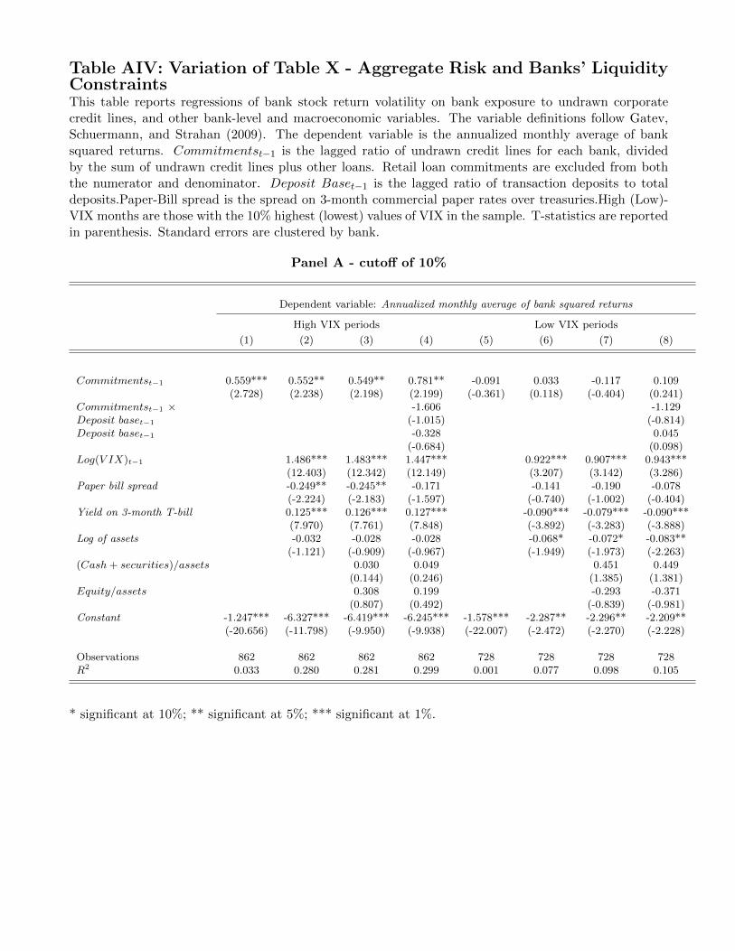
Table AIV: Variation of Table X - Aggregate Risk and Banks’ LiquidityConstraintsThis table reports regressions of bank stock return volatility on bank exposure to undrawn corporatecredit lines, and other bank-level and macroeconomic variables. The variable definitions follow Gatev,Schuermann, and Strahan (2009). The dependent variable is the annualized monthly average of banksquared returns. Commitmentst−1 is the lagged ratio of undrawn credit lines for each bank, dividedby the sum of undrawn credit lines plus other loans. Retail loan commitments are excluded from boththe numerator and denominator. Deposit Baset−1 is the lagged ratio of transaction deposits to totaldeposits.Paper-Bill spread is the spread on 3-month commercial paper rates over treasuries.High (Low)-VIX months are those with the 10% highest (lowest) values of VIX in the sample. T-statistics are reportedin parenthesis. Standard errors are clustered by bank.

Panel A - cutoff of 10%



(1) (2) (3) (4) (5) (6) (7) (8)

Commitmentst−1 0.559*** 0.552** 0.549** 0.781** -0.091 0.033 -0.117 0.109(2.728) (2.238) (2.198) (2.199) (-0.361) (0.118) (-0.404) (0.241)

Commitmentst−1 × -1.606 -1.129Deposit baset−1 (-1.015) (-0.814)Deposit baset−1 -0.328 0.045

(-0.684) (0.098)Log(V IX)t−1 1.486*** 1.483*** 1.447*** 0.922*** 0.907*** 0.943***

(12.403) (12.342) (12.149) (3.207) (3.142) (3.286)Paper bill spread -0.249** -0.245** -0.171 -0.141 -0.190 -0.078

(-2.224) (-2.183) (-1.597) (-0.740) (-1.002) (-0.404)Yield on 3-month T-bill 0.125*** 0.126*** 0.127*** -0.090*** -0.079*** -0.090***

(7.970) (7.761) (7.848) (-3.892) (-3.283) (-3.888)Log of assets -0.032 -0.028 -0.028 -0.068* -0.072* -0.083**


(0.144) (0.246) (1.385) (1.381)Equity/assets 0.308 0.199 -0.293 -0.371

(0.807) (0.492) (-0.839) (-0.981)Constant -1.247*** -6.327*** -6.419*** -6.245*** -1.578*** -2.287** -2.296** -2.209**

(-20.656) (-11.798) (-9.950) (-9.938) (-22.007) (-2.472) (-2.270) (-2.228)

Observations 862 862 862 862 728 728 728 728R2 0.033 0.280 0.281 0.299 0.001 0.077 0.098 0.105


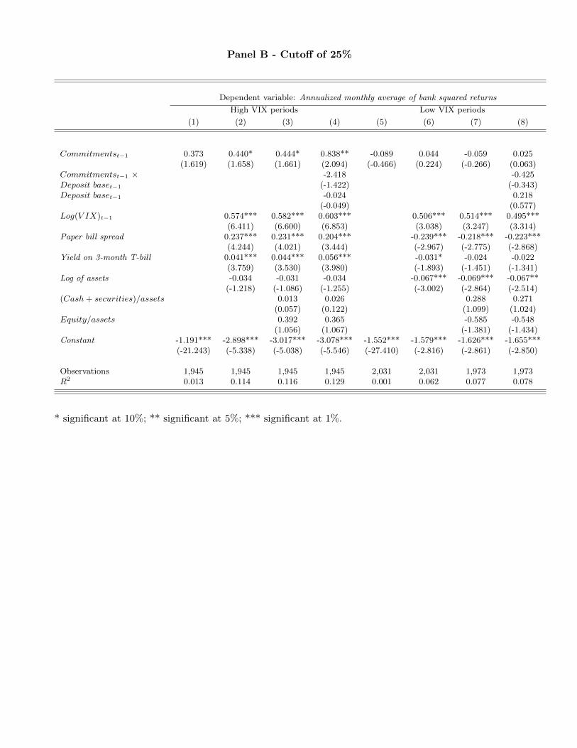
Panel B - Cutoff of 25%



(1) (2) (3) (4) (5) (6) (7) (8)

Commitmentst−1 0.373 0.440* 0.444* 0.838** -0.089 0.044 -0.059 0.025(1.619) (1.658) (1.661) (2.094) (-0.466) (0.224) (-0.266) (0.063)

Commitmentst−1 × -2.418 -0.425Deposit baset−1 (-1.422) (-0.343)Deposit baset−1 -0.024 0.218

(-0.049) (0.577)Log(V IX)t−1 0.574*** 0.582*** 0.603*** 0.506*** 0.514*** 0.495***

(6.411) (6.600) (6.853) (3.038) (3.247) (3.314)Paper bill spread 0.237*** 0.231*** 0.204*** -0.239*** -0.218*** -0.223***

(4.244) (4.021) (3.444) (-2.967) (-2.775) (-2.868)Yield on 3-month T-bill 0.041*** 0.044*** 0.056*** -0.031* -0.024 -0.022

(3.759) (3.530) (3.980) (-1.893) (-1.451) (-1.341)Log of assets -0.034 -0.031 -0.034 -0.067*** -0.069*** -0.067**


(0.057) (0.122) (1.099) (1.024)Equity/assets 0.392 0.365 -0.585 -0.548

(1.056) (1.067) (-1.381) (-1.434)Constant -1.191*** -2.898*** -3.017*** -3.078*** -1.552*** -1.579*** -1.626*** -1.655***

(-21.243) (-5.338) (-5.038) (-5.546) (-27.410) (-2.816) (-2.861) (-2.850)

Observations 1,945 1,945 1,945 1,945 2,031 2,031 1,973 1,973R2 0.013 0.114 0.116 0.129 0.001 0.062 0.077 0.078


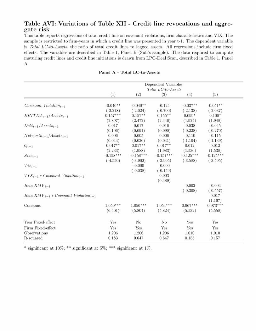
Table AVI: Variations of Table XII - Credit line revocations and aggre-gate riskThis table reports regressions of total credit line on covenant violations, firm characteristics and VIX. Thesample is restricted to firm-years in which a credit line was presented in year t-1. The dependent variableis Total LC-to-Assets, the ratio of total credit lines to lagged assets. All regressions include firm fixedeffects. The variables are described in Table 1, Panel B (Sufi’s sample). The data required to computematuring credit lines and credit line initiations is drawn from LPC-Deal Scan, described in Table 1, PanelA

Panel A - Total LC-to-Assets

Dependent Variables:Total LC-to-Assets

(1) (2) (3) (4) (5)

Covenant Violationt−1 -0.040** -0.040** -0.124 -0.037** -0.051**(-2.278) (-2.024) (-0.700) (-2.138) (-2.037)

EBITDAt−1/Assetst−1 0.157*** 0.157** 0.155** 0.099* 0.100*(2.897) (2.472) (2.446) (1.924) (1.948)

Debtt−1/Assetst−1 0.017 0.017 0.016 -0.038 -0.045(0.106) (0.091) (0.090) (-0.228) (-0.270)

Networtht−1/Assetst−1 0.006 0.005 0.006 -0.110 -0.115(0.044) (0.036) (0.041) (-1.104) (-1.139)

Qt−1 0.017** 0.017** 0.017** 0.012 0.012(2.233) (1.988) (1.983) (1.530) (1.538)

Sizet−1 -0.158*** -0.158*** -0.157*** -0.125*** -0.125***(-4.550) (-3.902) (-3.905) (-3.588) (-3.595)

V ixt−1 -0.000 -0.000(-0.038) (-0.159)

V IXt−1 ∗ Covenant Violationt−1 0.003(0.489)

Beta KMV t−1 -0.002 -0.004(-0.308) (-0.557)

Beta KMV t−1 ∗ Covenant Violationt−1 0.017(1.167)

Constant 1.050*** 1.050*** 1.054*** 0.967*** 0.973***(6.401) (5.804) (5.824) (5.532) (5.558)




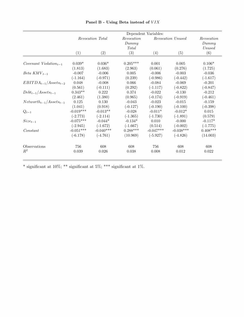
Panel B - Using Beta instead of V IX


DummyTotal


(1) (2) (3) (4) (5) (6)

Covenant Violationt−1 0.039* 0.036* 0.205*** 0.001 0.005 0.106*(1.813) (1.683) (2.963) (0.061) (0.276) (1.725)

Beta KMV t−1 -0.007 -0.006 0.005 -0.006 -0.003 -0.036(-1.164) (-0.971) (0.239) (-0.986) (-0.442) (-1.617)

EBITDAt−1/Assetst−2 0.048 -0.008 0.066 -0.084 -0.069 -0.201(0.561) (-0.111) (0.292) (-1.117) (-0.822) (-0.847)

Debtt−1/Assetst−1 0.343** 0.222 0.374 -0.022 -0.130 -0.212(2.461) (1.380) (0.965) (-0.174) (-0.919) (-0.461)

Networtht−1/Assetst−1 0.125 0.130 -0.043 -0.023 -0.015 -0.159(1.041) (0.918) (-0.127) (-0.190) (-0.100) (-0.398)

Qt−1 -0.019*** -0.013** -0.028 -0.011* -0.012* 0.015(-2.773) (-2.114) (-1.365) (-1.730) (-1.891) (0.579)

Sizet−1 -0.075*** -0.044* -0.134* 0.010 -0.000 -0.117*(-2.945) (-1.672) (-1.667) (0.514) (-0.002) (-1.775)

Constant -0.051*** -0.040*** 0.288*** -0.047*** -0.038*** 0.408***(-6.178) (-4.761) (10.969) (-5.927) (-4.826) (14.003)

Observations 756 608 608 756 608 608R2 0.039 0.026 0.038 0.008 0.012 0.022


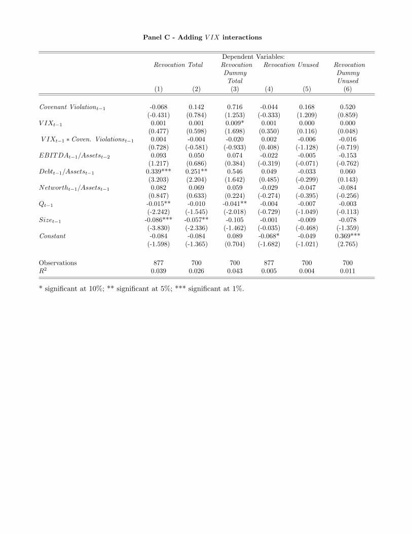
Panel C - Adding V IX interactions


DummyTotal


(1) (2) (3) (4) (5) (6)

Covenant Violationt−1 -0.068 0.142 0.716 -0.044 0.168 0.520(-0.431) (0.784) (1.253) (-0.333) (1.209) (0.859)

V IXt−1 0.001 0.001 0.009* 0.001 0.000 0.000(0.477) (0.598) (1.698) (0.350) (0.116) (0.048)

V IXt−1 ∗ Coven. Violationst−1 0.004 -0.004 -0.020 0.002 -0.006 -0.016(0.728) (-0.581) (-0.933) (0.408) (-1.128) (-0.719)

EBITDAt−1/Assetst−2 0.093 0.050 0.074 -0.022 -0.005 -0.153(1.217) (0.686) (0.384) (-0.319) (-0.071) (-0.762)

Debtt−1/Assetst−1 0.339*** 0.251** 0.546 0.049 -0.033 0.060(3.203) (2.204) (1.642) (0.485) (-0.299) (0.143)

Networtht−1/Assetst−1 0.082 0.069 0.059 -0.029 -0.047 -0.084(0.847) (0.633) (0.224) (-0.274) (-0.395) (-0.256)

Qt−1 -0.015** -0.010 -0.041** -0.004 -0.007 -0.003(-2.242) (-1.545) (-2.018) (-0.729) (-1.049) (-0.113)

Sizet−1 -0.086*** -0.057** -0.105 -0.001 -0.009 -0.078(-3.830) (-2.336) (-1.462) (-0.035) (-0.468) (-1.359)

Constant -0.084 -0.084 0.089 -0.068* -0.049 0.369***(-1.598) (-1.365) (0.704) (-1.682) (-1.021) (2.765)

Observations 877 700 700 877 700 700R2 0.039 0.026 0.043 0.005 0.004 0.011


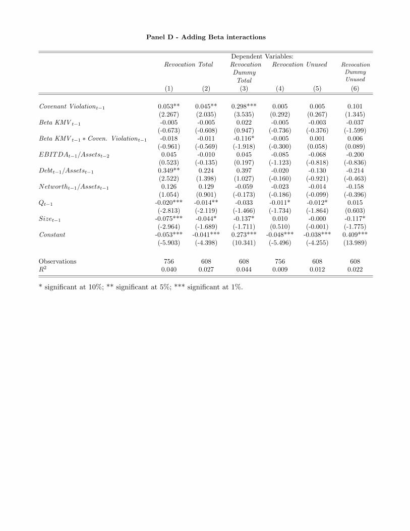
Panel D - Adding Beta interactions


DummyTotal


(1) (2) (3) (4) (5) (6)

Covenant Violationt−1 0.053** 0.045** 0.298*** 0.005 0.005 0.101(2.267) (2.035) (3.535) (0.292) (0.267) (1.345)

Beta KMV t−1 -0.005 -0.005 0.022 -0.005 -0.003 -0.037(-0.673) (-0.608) (0.947) (-0.736) (-0.376) (-1.599)

Beta KMV t−1 ∗ Coven. Violationt−1 -0.018 -0.011 -0.116* -0.005 0.001 0.006(-0.961) (-0.569) (-1.918) (-0.300) (0.058) (0.089)

EBITDAt−1/Assetst−2 0.045 -0.010 0.045 -0.085 -0.068 -0.200(0.523) (-0.135) (0.197) (-1.123) (-0.818) (-0.836)

Debtt−1/Assetst−1 0.349** 0.224 0.397 -0.020 -0.130 -0.214(2.522) (1.398) (1.027) (-0.160) (-0.921) (-0.463)

Networtht−1/Assetst−1 0.126 0.129 -0.059 -0.023 -0.014 -0.158(1.054) (0.901) (-0.173) (-0.186) (-0.099) (-0.396)

Qt−1 -0.020*** -0.014** -0.033 -0.011* -0.012* 0.015(-2.813) (-2.119) (-1.466) (-1.734) (-1.864) (0.603)

Sizet−1 -0.075*** -0.044* -0.137* 0.010 -0.000 -0.117*(-2.964) (-1.689) (-1.711) (0.510) (-0.001) (-1.775)

Constant -0.053*** -0.041*** 0.273*** -0.048*** -0.038*** 0.409***(-5.903) (-4.398) (10.341) (-5.496) (-4.255) (13.989)

Observations 756 608 608 756 608 608R2 0.040 0.027 0.044 0.009 0.012 0.022


Documents

Aggregate Risk and the Choice between Cash and Lines · PDF fileAggregate Risk and the Choice between Cash and Lines of Credit VIRAL V. ACHARYA, HEITOR ALMEIDA, and, MURILLO CAMPELLO