Aggregate Supply

Chapter 11-3 Aggregate Supply

Aggregate Supply

• The aggregate supply curve shows the relationship between the aggregate price level and the quantity of aggregate output.

Aggregate Supply Curve• Aggregate Supply is the amount of real GDP

that will be made available by sellers at various price levels.

• Aggregate Supply looks different in the Long Run and the Short Run:– In the Long Run, classical economists assume the

economy operates at full employment (maximum output), independent of the price level.

– In the Short Run, businesses will increase supply if the price level increases.

Positive Relationship

• There is a positive relationship in the short run between price level and the quantity of aggregate output supplied.

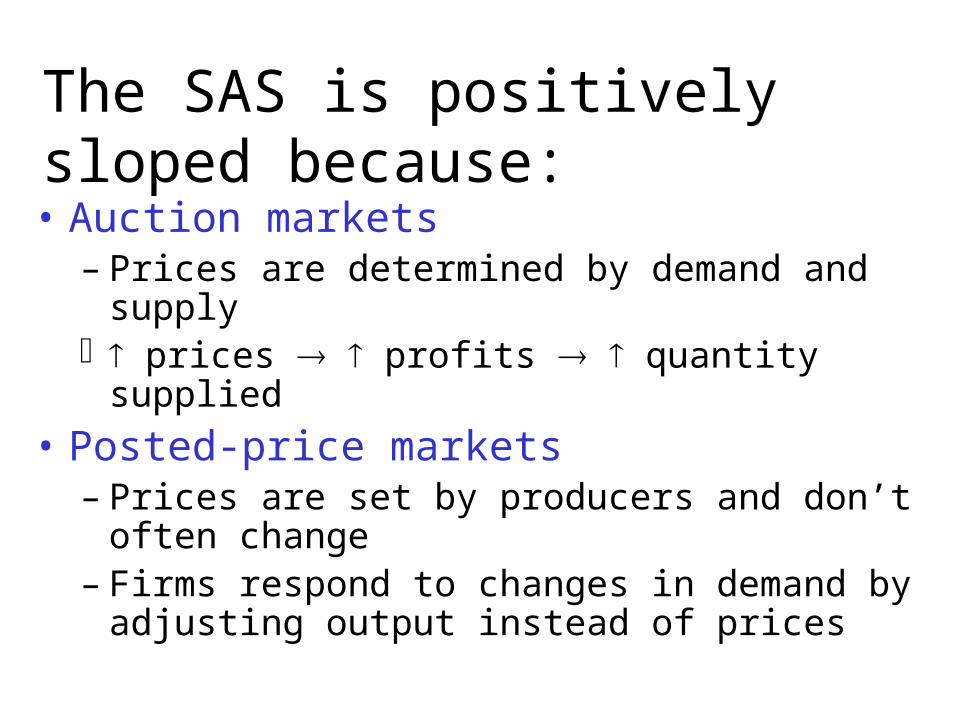
The SAS is positively sloped because:• Auction markets

– Prices are determined by demand and supply prices profits quantity supplied

• Posted-price markets– Prices are set by producers and don’t often

change– Firms respond to changes in demand by

adjusting output instead of prices

Sticky Nominal Wages

• The short-run aggregate supply curve is upward-sloping because nominal wages are sticky in the short run: – a higher aggregate price level leads to higher profits

and increased aggregate output in the short run.

• The nominal wage is the dollar amount of the wage paid.

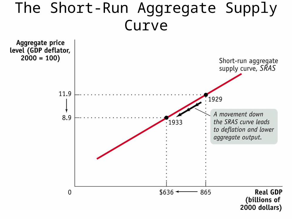
The Short-Run Aggregate Supply Curve

Movement Vs. Shift

• Movements are caused by change in Aggregate Price Levels

• Shift in SRAS is caused by:

Shift in SRAS

• Changes in – commodity prices, – nominal wages, and – productivity

• lead to changes in producers’ profits and shift the short-run aggregate supply curve

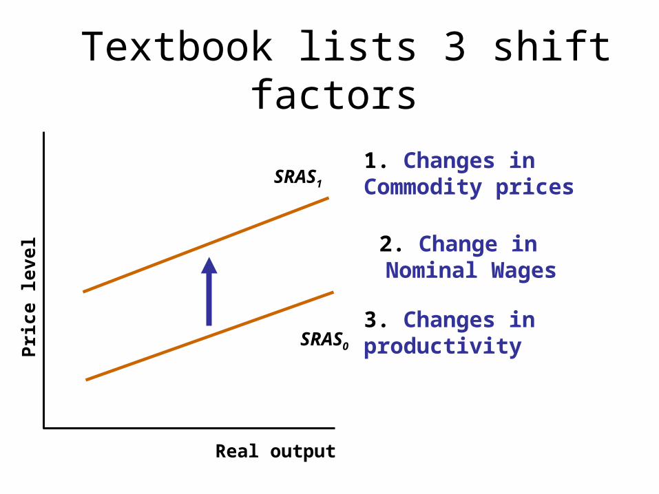
Textbook lists 3 shift factors

Real output

Pri

ce

lev

el

SRAS0

SRAS1

1. Changes in Commodity prices

3. Changes in productivity

2. Change in Nominal Wages

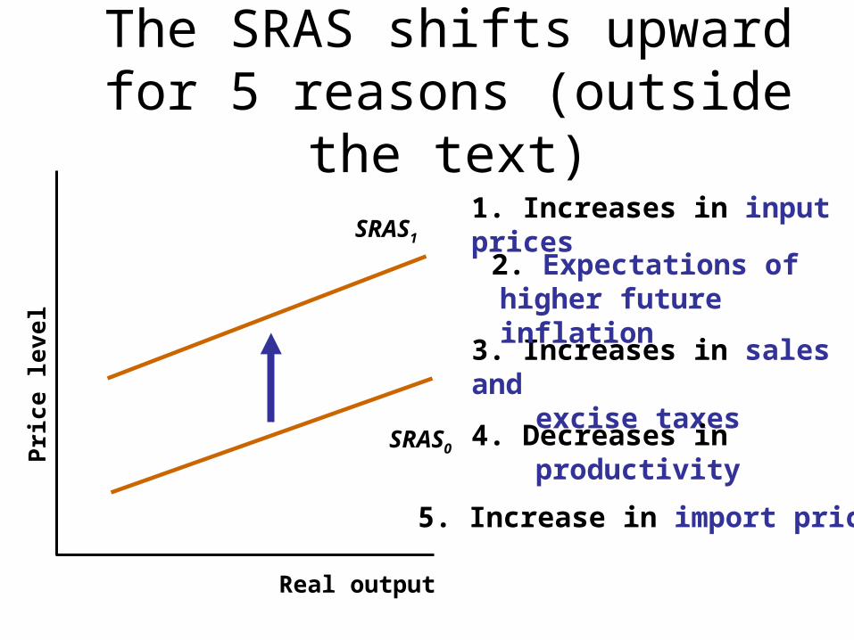
The SRAS shifts upward for 5 reasons (outside the text)

Real output

Pri

ce

lev

el

SRAS0

SRAS1

1. Increases in input prices

3. Increases in sales and excise taxes

2. Expectations of higher future inflation

4. Decreases in productivity

5. Increase in import prices

LRAS

• The long-run aggregate supply curve shows the relationship between the aggregate price level and the quantity of aggregate output supplied that would exist if all prices, including nominal wages, were fully flexible

A Range for Potential Output and the LAS Curve

• The position of the long-run aggregate supply curve is determined by potential output.

• Potential output – the amount of goods and services an economy can produce when both labor and capital are fully employed.

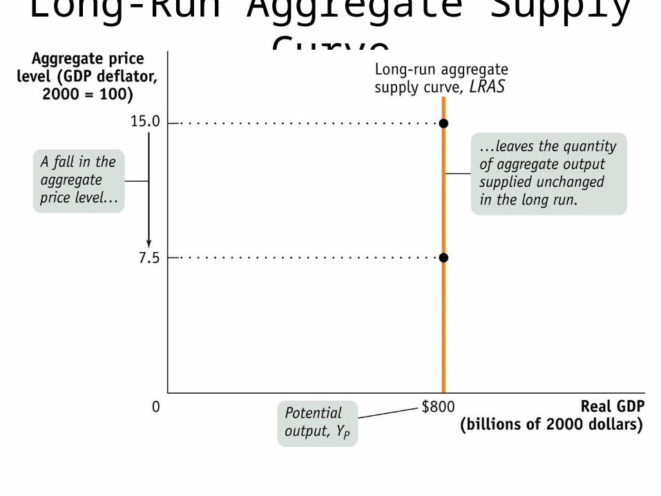
Long-Run Aggregate Supply Curve

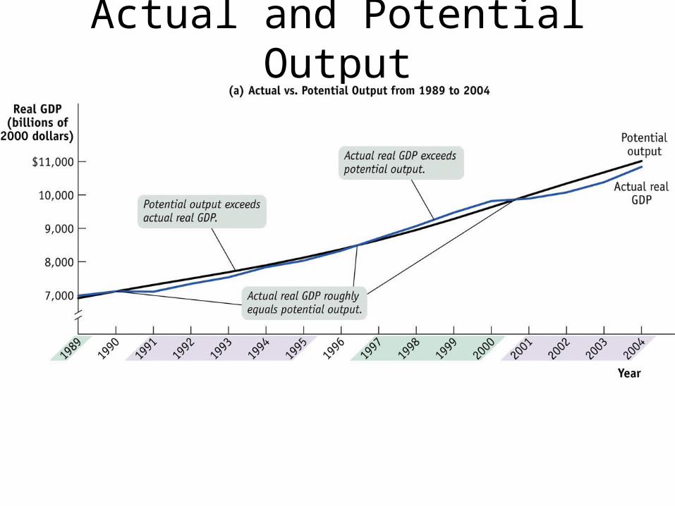
Actual and Potential Output

Economic Growth Shifts the LRAS Curve Rightward

Real output

Pri

ce L

evel

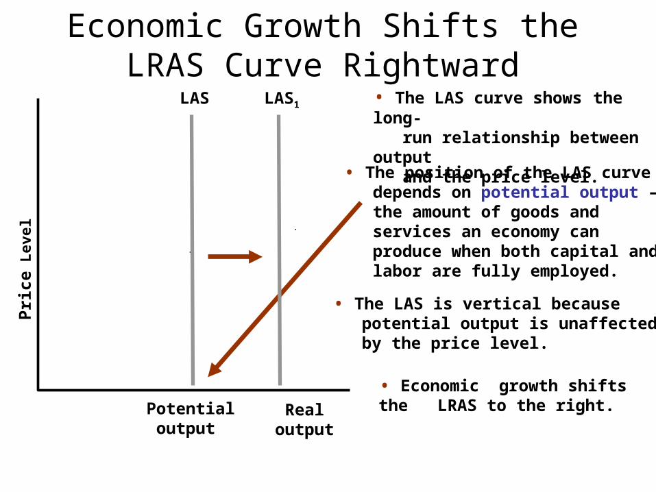
LAS • The LAS curve shows the long- run relationship between output and the price level.

• Economic growth shifts the LRAS to the right.

• The LAS is vertical because potential output is unaffected by the price level.

• The position of the LAS curve depends on potential output – the amount of goods and services an economy can produce when both capital and labor are fully employed.

Potential output

LAS1

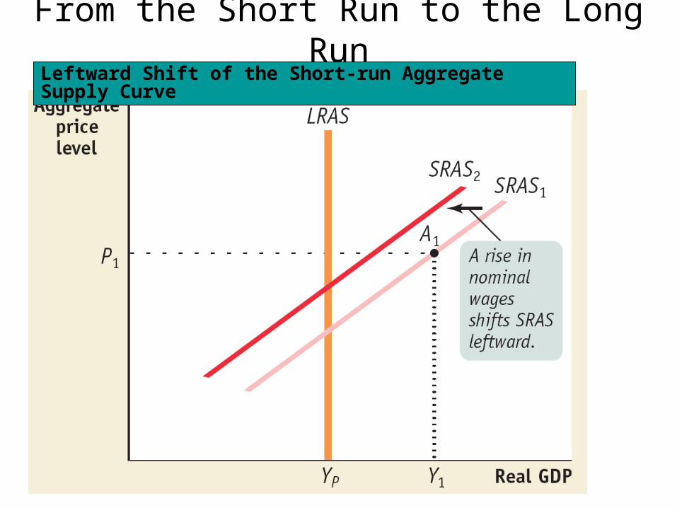
From the Short Run to the Long RunLeftward Shift of the Short-run Aggregate Supply Curve

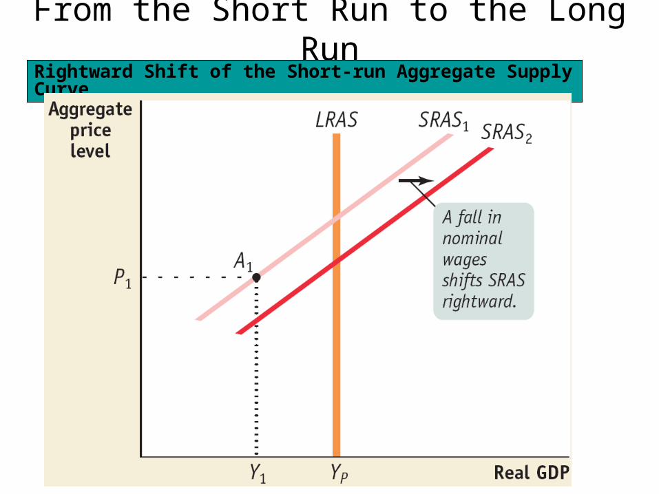
From the Short Run to the Long RunRightward Shift of the Short-run Aggregate Supply Curve

LAS Curve

Real output

Pri

ce L

evel

Low-level

potential output

High-level potential output

C

SAS

B

A

LAS

Underutilizedresources

Overutilizedresources

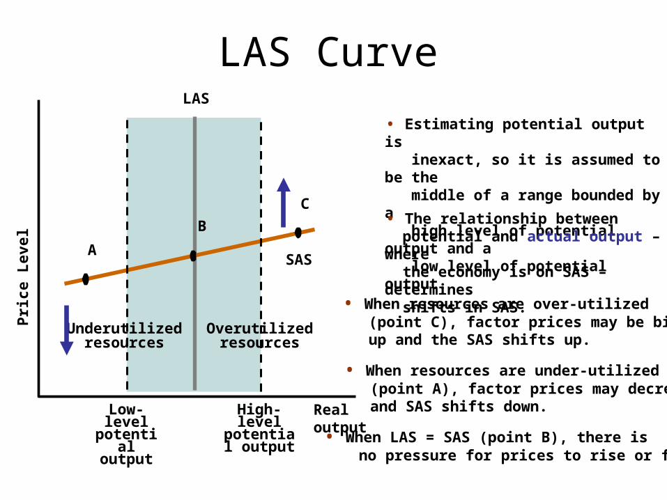
• Estimating potential output is inexact, so it is assumed to be the middle of a range bounded by a high level of potential output and a low level of potential output.

• The relationship between potential and actual output – where the economy is on SAS – determines shifts in SAS.

• When LAS = SAS (point B), there is no pressure for prices to rise or fall.

• When resources are over-utilized (point C), factor prices may be bid up and the SAS shifts up.

• When resources are under-utilized (point A), factor prices may decrease and SAS shifts down.

The Following Slides

are from your textbook.

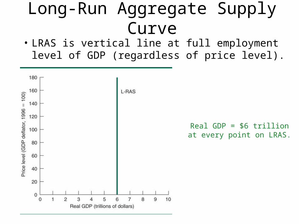
Long-Run Aggregate Supply Curve

• LRAS is vertical line at full employment level of GDP (regardless of price level).

Real GDP = $6 trillionat every point on LRAS.

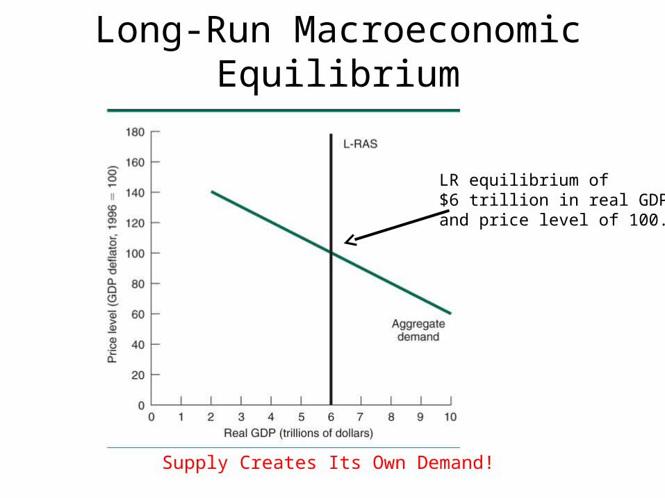
Long-Run Macroeconomic Equilibrium

LR equilibrium of $6 trillion in real GDPand price level of 100.

Supply Creates Its Own Demand!

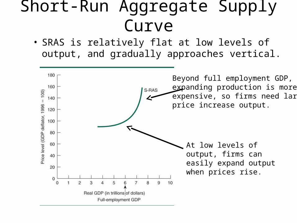
Short-Run Aggregate Supply Curve

• SRAS is relatively flat at low levels of output, and gradually approaches vertical.

At low levels of output, firms can easily expand output when prices rise.

Beyond full employment GDP,expanding production is moreexpensive, so firms need largeprice increase output.