Embed Size (px)
Citation preview
Agilent X-Series Signal Analyzer
Spectrum Analyzer Mode Measurement Guide
This manual provides documentation for the following X-Series Analyzers: PXA Signal Analyzer N9030A MXA Signal Analyzer N9020A EXA Signal Analyzer N9010A CXA Signal Analyzer N9000A
Notices© Agilent Technologies, Inc. 2008-2009
No part of this manual may be reproduced in any form or by any means (including electronic storage and retrieval or transla-tion into a foreign language) without prior agreement and written consent from Agi-lent Technologies, Inc. as governed by United States and international copyright laws.
Manual Part NumberN9060-90032 Supersedes: N9060-90030
Print DateNovember 2010
Printed in USA
Agilent Technologies, Inc. 1400 Fountaingrove Parkway Santa Rosa, CA 95403
WarrantyThe material contained in this doc-ument is provided “as is,” and is subject to being changed, without notice, in future editions. Further, to the maximum extent permitted by applicable law, Agilent disclaims all warranties, either express or implied, with regard to this manual and any information contained herein, including but not limited to the implied warranties of mer-chantability and fitness for a par-ticular purpose. Agilent shall not be liable for errors or for incidental or consequential damages in con-nection with the furnishing, use, or performance of this document or of any information contained herein. Should Agilent and the user have a separate written agreement with warranty terms covering the mate-rial in this document that conflict with these terms, the warranty terms in the separate agreement shall control.
Technology Licenses The hardware and/or software described in this document are furnished under a license and may be used or copied only in accordance with the terms of such license.
Restricted Rights LegendIf software is for use in the performance of a U.S. Government prime contract or subcontract, Software is delivered and
licensed as “Commercial computer soft-ware” as defined in DFAR 252.227-7014 (June 1995), or as a “commercial item” as defined in FAR 2.101(a) or as “Restricted computer software” as defined in FAR 52.227-19 (June 1987) or any equivalent agency regulation or contract clause. Use, duplication or disclosure of Software is subject to Agilent Technologies’ standard commercial license terms, and non-DOD Departments and Agencies of the U.S. Government will receive no greater than Restricted Rights as defined in FAR 52.227-19(c)(1-2) (June 1987). U.S. Gov-ernment users will receive no greater than Limited Rights as defined in FAR 52.227-14 (June 1987) or DFAR 252.227-7015 (b)(2) (November 1995), as applicable in any technical data.
Safety Notices
CAUTION
A CAUTION notice denotes a hazard. It calls attention to an operating procedure, practice, or the like that, if not correctly per-formed or adhered to, could result in damage to the product or loss of important data. Do not proceed beyond a CAUTION notice until the indicated conditions are fully understood and met.
WARNING
A WARNING notice denotes a hazard. It calls attention to an operating procedure, practice, or the like that, if not correctly performed or adhered to, could result in personal injury or death. Do not proceed beyond a WARNING notice until the indi-cated conditions are fully understood and met.
2
Trademark Acknowledgements
Microsoft® is a U.S. registered trademark of Microsoft Corporation.
Windows® and MS Windows® are U.S. registered trademarks of Microsoft Corporation.
Adobe Reader® is a U.S. registered trademark of Adobe System Incorporated.
Java™ is a U.S. trademark of Sun Microsystems, Inc.
MATLAB® is a U.S. registered trademark of Math Works, Inc.
Norton Ghost™ is a U.S. trademark of Symantec Corporation.
3
WarrantyThis Agilent technologies instrument product is warranted against defects in material and workmanship for a period of one year from the date of shipment. During the warranty period, Agilent Technologies will, at its option, either repair or replace products that prove to be defective.
For warranty service or repair, this product must be returned to a service facility designated by Agilent Technologies. Buyer shall prepay shipping charges to Agilent Technologies and Agilent Technologies shall pay shipping charges to return the product to Buyer. However, Buyer shall pay all shipping charges, duties, and taxes for products returned to Agilent Technologies from another country.
Where to Find the Latest InformationDocumentation is updated periodically. For the latest information about this analyzer, including firmware upgrades, application information, and product information, see the following URLs:
http://www.agilent.com/find/pxa http://www.agilent.com/find/mxa http://www.agilent.com/find/exa http://www.agilent.com/find/cxa
To receive the latest updates by email, subscribe to Agilent Email Updates:
http://www.agilent.com/find/emailupdates
Information on preventing analyzer damage can be found at:
http://www.agilent.com/find/tips

4
Contents
5
1 Getting Started with the Spectrum Analyzer Measurement ApplicationMaking a Basic Measurement 10
Using the Front Panel 10Presetting the Signal Analyzer 11Viewing a Signal 12
Recommended Test Equipment 15Accessories Available 16
50 Ohm Load 1650 Ohm/75 Ohm Minimum Loss Pad 1675 Ohm Matching Transformer 16AC Probe 16AC Probe (Low Frequency) 16Broadband Preamplifiers and Power Amplifiers 17GPIB Cable 17USB/GPIB Cable 17RF and Transient Limiters 17Power Splitters 18Static Safety Accessories 18
2 Measuring Multiple SignalsComparing Signals on the Same Screen Using Marker Delta 20Comparing Signals not on the Same Screen Using Marker Delta 23Resolving Signals of Equal Amplitude 26Resolving Small Signals Hidden by Large Signals 31Decreasing the Frequency Span Around the Signal 35Easily Measure Varying Levels of Modulated Power Compared to a Reference 37
3 Measuring a Low−Level SignalReducing Input Attenuation 42Decreasing the Resolution Bandwidth 45Using the Average Detector and Increased Sweep Time 48Trace Averaging 50
6
Contents
4 Improving Frequency Resolution and AccuracyUsing a Frequency Counter to Improve Frequency Resolution and Accuracy 54
5 Tracking Drifting Signals Measuring a Source Frequency Drift 56Tracking a Signal 59
6 Making Distortion MeasurementsIdentifying Analyzer Generated Distortion 62Third-Order Intermodulation Distortion 65
7 Measuring NoiseMeasuring Signal-to-Noise 70Measuring Noise Using the Noise Marker 72Measuring Noise-Like Signals Using Band/Interval Density Markers 76Measuring Noise-Like Signals Using the Channel Power Measurement 79Measuring Signal-to-Noise of a Modulated Carrier 81Improving Phase Noise Measurements by Subtracting Signal Analyzer Noise 86
8 Making Time-Gated MeasurementsGenerating a Pulsed-RF FM Signal 92
Signal source setup 92Analyzer Setup 93Digitizing oscilloscope setup 95
Connecting the Instruments to Make Time-Gated Measurements 97Gated LO Measurement 98Gated Video Measurement 102Gated FFT Measurement 106
9 Measuring Digital Communications SignalsChannel Power Measurements 110Occupied Bandwidth Measurements 112
Troubleshooting Hints 113

Contents
7
Making Adjacent Channel Power (ACP) Measurements 114Making Statistical Power Measurements (CCDF) 119Making Burst Power Measurements 124Spurious Emissions Measurements 130
Troubleshooting Hints 132Spectrum Emission Mask Measurements 133
Troubleshooting Hints 134
10 Demodulating AM SignalsMeasuring the Modulation Rate of an AM Signal 138Measuring the Modulation Index of an AM Signal 142
11 IQ Analyzer MeasurementCapturing wideband signals for further analysis 146Complex Spectrum Measurement 147IQ Waveform (Time Domain) Measurement 149
12 Using Option BBA Baseband I/Q InputsBaseband I/Q Measurements Available for X-Series Signal Analyzers 154Baseband I/Q Measurement Overview 155
13 ConceptsResolving Closely Spaced Signals 158
Resolving Signals of Equal Amplitude 158Resolving Small Signals Hidden by Large Signals 158
Trigger Concepts 160Selecting a Trigger 160
Time Gating Concepts 164Introduction: Using Time Gating on a Simplified Digital Radio Signal 164How Time Gating Works 166Measuring a Complex/Unknown Signal 172“Quick Rules” for Making Time-Gated Measurements 177Using the Edge Mode or Level Mode for Triggering 180

8
Contents
Noise Measurements Using Time Gating 181AM and FM Demodulation Concepts 182
Demodulating an AM Signal Using the Analyzer as a Fixed Tuned Receiver (Time-Domain) 182Demodulating an FM Signal Using the Analyzer as a Fixed Tuned Receiver (Time-Domain) 182
IQ Analysis Concepts 183Purpose 183Complex Spectrum Measurement 183IQ Waveform Measurement 183
Spurious Emissions Measurement Concepts 185Purpose 185Measurement Method 185
Spectrum Emission Mask Measurement Concepts 186Purpose 186Measurement Method 186
Occupied Bandwidth Measurement Concepts 187Purpose 187Measurement Method 187
Baseband I/Q Inputs (Option BBA) Measurement Concepts 188What are Baseband I/Q Inputs? 188What are Baseband I/Q Signals? 188Why Make Measurements at Baseband? 189Selecting Input Probes for Baseband Measurements 190Baseband I/Q Measurement Views 191
9
Getting Started with the Spectrum Analyzer Measurement Application
1 Getting Started with the Spectrum Analyzer Measurement Application
This chapter provides some basic information about using the Spectrum Analyzer and IQ Analyzer Measurement Application Modes. It includes topics on:
• “Making a Basic Measurement” on page 10
• “Recommended Test Equipment” on page 15
• “Accessories Available” on page 16
Technical Documentation Summary:
Your Signal Analysis measurement platform:
Getting Started Turn on process, Windows XP use/configuration, Front and rear panel
Specifications Specifications for all available Measurement Applications and optional hardware (for example, Spectrum Analyzer and W-CDMA)
Functional Testing Quick checks to verify overall instrument operation.
Instrument Messages Descriptions of displayed messages of Information, Warnings and Errors
Measurement Application specific documentation: (for example, Spectrum Analyzer Measurement Application or W-CDMA Measurement Application)
Measurement Guide Examples of measurements made using the front panel keys or over a remote interface.
User’s/Programmer’s Reference
Descriptions of front panel key functionality and the corresponding SCPI commands. May also include some concept information.

10
Getting Started with the Spectrum Analyzer Measurement ApplicationMaking a Basic Measurement
Making a Basic MeasurementRefer to the description of the instrument front and rear panels to improve your understanding of the Agilent Signal Analyzer measurement platform. This knowledge will help you with the following measurement example.
This section includes:
• “Using the Front Panel” on page 10
• “Presetting the Signal Analyzer” on page 11
• “Viewing a Signal” on page 12
CAUTION Make sure that the total power of all signals at the analyzer input does not exceed +30 dBm (1 watt).
Using the Front Panel
Entering DataWhen setting measurement parameters, there are several ways to enter or modify the value of the active function:
Using Menu KeysMenu Keys (which appear along the right side of the display) provide access to many analyzer functions. Here are examples of menu key types:
Knob Increments or decrements the current value.
Arrow Keys Increments or decrements the current value.
Numeric Keypad Enters a specific value. Then press the desired terminator (either a unit softkey, or the Enter key).
Unit Softkeys Terminate a value that requires a unit-of-measurement.
Enter Key Terminates an entry when either no unit of measure is needed, or you want to use the default unit.
Toggle Allows you to activate/deactivate states.
Example: Toggles the selection (underlined choice) each time you press the key.
Submenu Displays a new menu of softkeys.
11
Getting Started with the Spectrum Analyzer Measurement ApplicationMaking a Basic Measurement
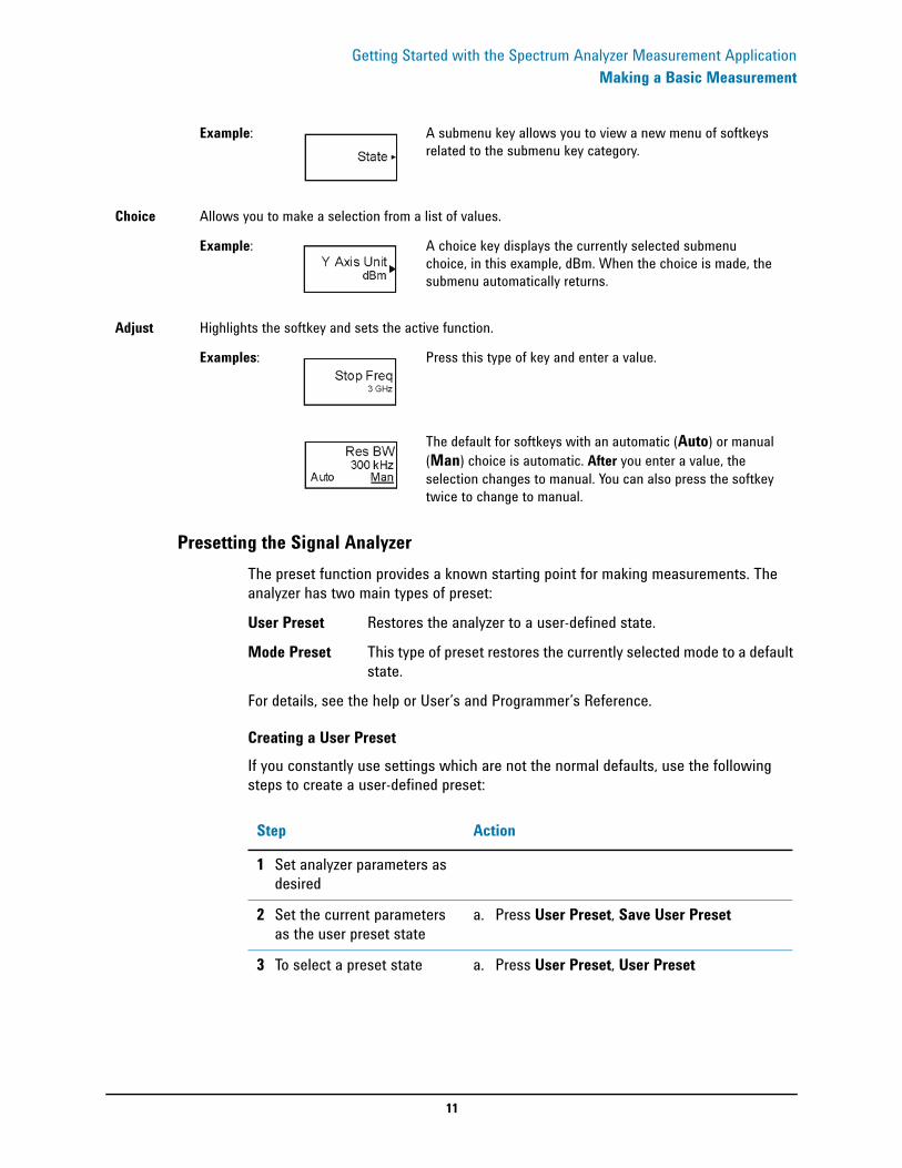
Presetting the Signal AnalyzerThe preset function provides a known starting point for making measurements. The analyzer has two main types of preset:
User Preset Restores the analyzer to a user-defined state.
Mode Preset This type of preset restores the currently selected mode to a default state.
For details, see the help or User’s and Programmer’s Reference.
Creating a User PresetIf you constantly use settings which are not the normal defaults, use the following steps to create a user-defined preset:
Example: A submenu key allows you to view a new menu of softkeys related to the submenu key category.
Choice Allows you to make a selection from a list of values.
Example: A choice key displays the currently selected submenu choice, in this example, dBm. When the choice is made, the submenu automatically returns.
Adjust Highlights the softkey and sets the active function.
Examples: Press this type of key and enter a value.
The default for softkeys with an automatic (Auto) or manual (Man) choice is automatic. After you enter a value, the selection changes to manual. You can also press the softkey twice to change to manual.
Step Action
1 Set analyzer parameters as desired
2 Set the current parameters as the user preset state
a. Press User Preset, Save User Preset
3 To select a preset state a. Press User Preset, User Preset

12
Getting Started with the Spectrum Analyzer Measurement ApplicationMaking a Basic Measurement
Viewing a Signal
Reading Frequency & Amplitude
Changing Reference Level
Step Action Notes
1 Return the current mode settings to factory defaults.
a. Press Mode Preset.
2 Route the internal 50 MHz signal to the analyzer input.
a. Press Input/Output, RF Calibrator, 50, MHz.
3 Set the reference level to 10 dBm.
a. Press AMPTD Y Scale, 10, dBm.
4 Set the center frequency to 40 MHz.
a. Press FREQ Channel, Center Freq, 40, MHz.
The 50 MHz reference signal appears on the display
5 Set the frequency span to 50 MHz.
a. Press SPAN, 50, MHz.
Step Action Notes
1 Activate a marker and place it on the highest amplitude signal.
a. Press Peak Search.
The frequency and amplitude of the marker appear in the active function block in the upper-right of the display. You can use the knob, the arrow keys, or the softkeys in the Peak Search menu to move the marker around on the signal.
2 To return the marker to the peak of the signal.
a. Press Peak Search.
Step Action Notes
1 Change the reference level.
a. Press AMPLTD Y Scale.
b. Press Marker −>, Mkr −> Ref Lvl.
The reference level is now the active function.
13
Getting Started with the Spectrum Analyzer Measurement ApplicationMaking a Basic Measurement
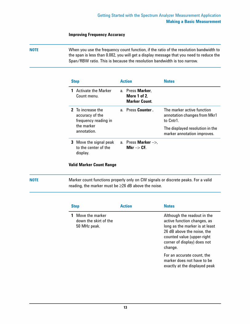
Improving Frequency Accuracy
NOTE When you use the frequency count function, if the ratio of the resolution bandwidth to the span is less than 0.002, you will get a display message that you need to reduce the Span/RBW ratio. This is because the resolution bandwidth is too narrow.
Valid Marker Count Range
NOTE Marker count functions properly only on CW signals or discrete peaks. For a valid reading, the marker must be ≥26 dB above the noise.
Step Action Notes
1 Activate the Marker Count menu.
a. Press Marker, More 1 of 2, Marker Count.
2 To increase the accuracy of the frequency reading in the marker annotation.
a. Press Counter . The marker active function annotation changes from Mkr1 to Cntr1.The displayed resolution in the marker annotation improves.
3 Move the signal peak to the center of the display.
a. Press Marker −>, Mkr −> CF.
Step Action Notes
1 Move the marker down the skirt of the 50 MHz peak.
Although the readout in the active function changes, as long as the marker is at least 26 dB above the noise, the counted value (upper-right corner of display) does not change.For an accurate count, the marker does not have to be exactly at the displayed peak
14
Getting Started with the Spectrum Analyzer Measurement ApplicationMaking a Basic Measurement
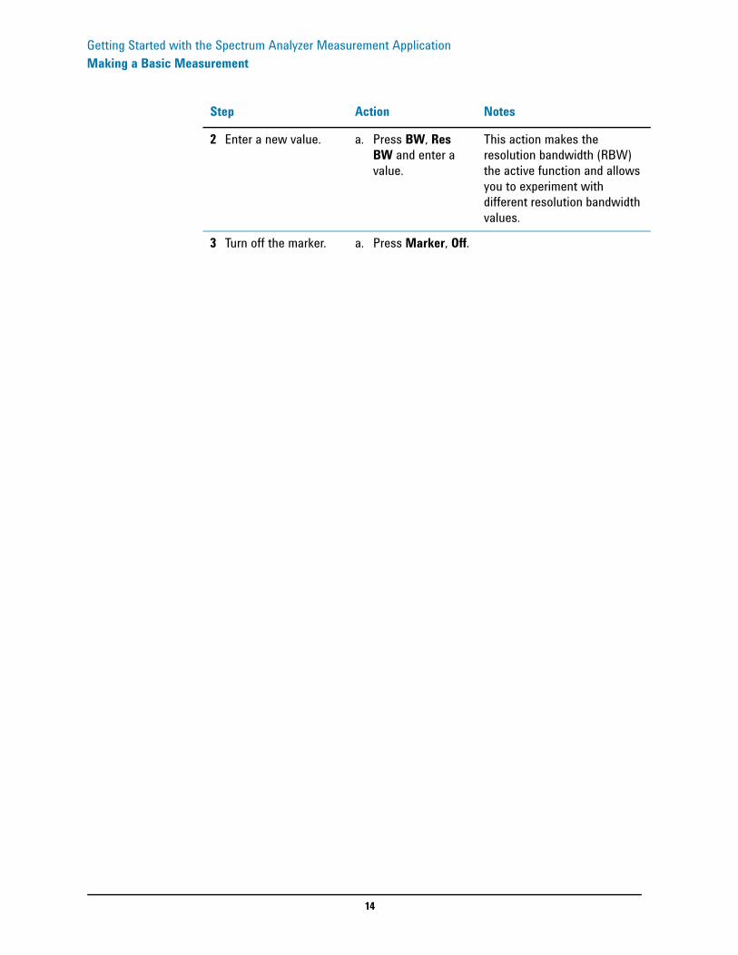
2 Enter a new value. a. Press BW, Res BW and enter a value.
This action makes the resolution bandwidth (RBW) the active function and allows you to experiment with different resolution bandwidth values.
3 Turn off the marker. a. Press Marker, Off.
Step Action Notes
15
Getting Started with the Spectrum Analyzer Measurement ApplicationRecommended Test Equipment
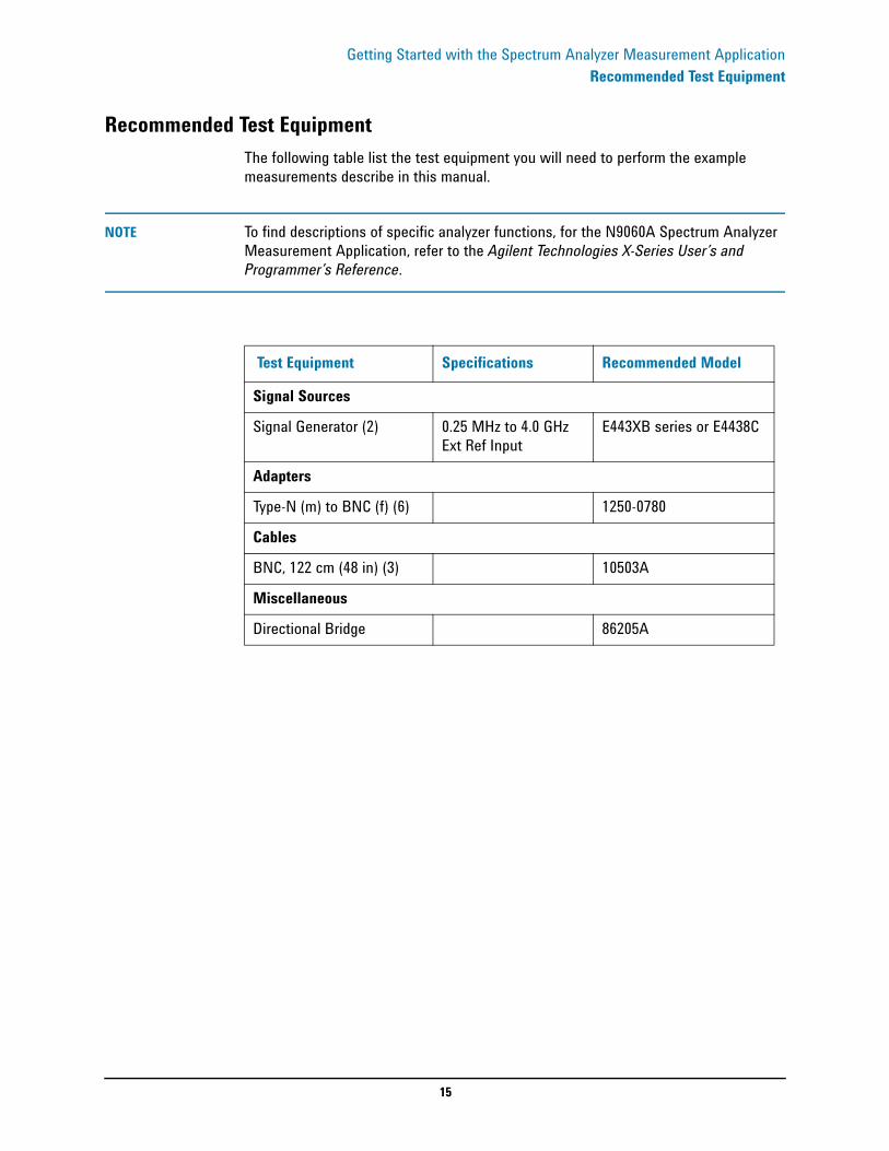
Recommended Test EquipmentThe following table list the test equipment you will need to perform the example measurements describe in this manual.
NOTE To find descriptions of specific analyzer functions, for the N9060A Spectrum Analyzer Measurement Application, refer to the Agilent Technologies X-Series User’s and Programmer’s Reference.
Test Equipment Specifications Recommended Model
Signal Sources
Signal Generator (2) 0.25 MHz to 4.0 GHz Ext Ref Input
E443XB series or E4438C
Adapters
Type-N (m) to BNC (f) (6) 1250-0780
Cables
BNC, 122 cm (48 in) (3) 10503A
Miscellaneous
Directional Bridge 86205A
16
Getting Started with the Spectrum Analyzer Measurement ApplicationAccessories Available
Accessories AvailableA number of accessories are available from Agilent Technologies to help you configure your analyzer for your specific applications. They can be ordered through your local Agilent Sales and Service Office and are listed below.
NOTE There are also some instrument options available that can improve your measurements. Some options can only be ordered when you make your original equipment purchase. But some are also available as kits that you can order and install later. Order kits through your local Agilent Sales and Service Office.
For the latest information on Agilent signal analyzer options and upgrade kits, visit the following Internet URL: http://www.agilent.com/find/sa_upgrades
50 Ohm LoadThe Agilent 909 series of loads come in several models and options providing a variety of frequency ranges and VSWRs. Also, they are available in either 50 ohm or 75 Ohm. Some examples include the:
909A: DC to 18 GHz909C: DC to 2 GHz909D: DC to 26.5 GHz
50 Ohm/75 Ohm Minimum Loss Pad The HP/Agilent 11852B is a low VSWR minimum loss pad that allows you to make measurements on 75 Ohm devices using an analyzer with a 50 Ohm input. It is effective over a frequency range of dc to 2 GHz.
75 Ohm Matching Transformer The HP/Agilent 11694A allows you to make measurements in 75 Ohm systems using an analyzer with a 50 Ohm input. It is effective over a frequency range of 3 to 500 MHz.
AC Probe The Agilent 85024A high frequency probe performs in-circuit measurements without adversely loading the circuit under test. The probe has an input capacitance of 0.7 pF shunted by 1 megohm of resistance and operates over a frequency range of 300 kHz to 3 GHz. High probe sensitivity and low distortion levels allow measurements to be made while taking advantage of the full dynamic range of the signal analyzer.
AC Probe (Low Frequency)The Agilent 41800A low frequency probe has a low input capacitance and a frequency range of 5 Hz to 500 MHz.

17
Getting Started with the Spectrum Analyzer Measurement ApplicationAccessories Available
Broadband Preamplifiers and Power Amplifiers Preamplifiers and power amplifiers can be used with your signal analyzer to enhance measurements of very low-level signals.
• The Agilent 8447D preamplifier provides a minimum of 25 dB gain from 100 kHz to 1.3 GHz.
• The Agilent 87405A preamplifier provides a minimum of 22 dB gain from 10 MHz to 3 GHz. (Power is supplied by the probe power output of the analyzer.)
• The Agilent 83006A preamplifier provides a minimum of 26 dB gain from 10 MHz to 26.5 GHz.
• The Agilent 85905A CATV 75 ohm preamplifier provides a minimum of 18 dB gain from 45 MHz to 1 GHz. (Power is supplied by the probe power output of the analyzer.)
• The 11909A low noise preamplifier provides a minimum of 32 dB gain from 9 kHz to 1 GHz and a typical noise figure of 1.8 dB.
GPIB Cable The Agilent 10833 Series GPIB cables interconnect GPIB devices and are available in four different lengths (0.5 to 4 meters). GPIB cables are used to connect controllers to a signal analyzer.
USB/GPIB Cable The Agilent 82357A USB/GPIB interface provides a direct connection from the USB port on your laptop or desktop PC to GPIB instruments. It comes with the SICL and VISA software for Windows® 2000/XP. Using VISA software, your existing GPIB programs work immediately, without modification. The 82357A is a standard Plug and Play device and you can interface with up to 14 GPIB instruments.
RF and Transient Limiters The Agilent 11867A and N9355B RF and Microwave Limiters protect the analyzer input circuits from damage due to high power levels. The N9355B operates over a frequency range of dc to 1800 MHz and begins reflecting signal levels over 1 mW up to 10 W average power and 100 watts peak power. The 11693A microwave limiter (0.1 to 18 GHz) guards against input signals over 10 milliwatt up to 1 watt average power.
The Agilent 11947A Transient Limiter protects the analyzer input circuits from damage due to signal transients. It specifically is needed for use with a line impedance stabilization network (LISN). It operates over a frequency range of 9 kHz to 200 MHz, with 10 dB of insertion loss.
18
Getting Started with the Spectrum Analyzer Measurement ApplicationAccessories Available
Power SplittersThe Agilent 11667A/B/C power splitters are two-resistor type splitters that provide excellent output SWR, at 50 Ω impedance. The tracking between the two output arms, over a broad frequency range, allows wideband measurements to be made with a minimum of uncertainty.
11667A: DC to 18 GHz11667B: DC to 26.5 GHz11667C: DC to 50 GHz
Static Safety Accessories9300-1367 Wrist-strap, color black, stainless steel. Four adjustable links and a
7 mm post-type connection.
9300-0980 Wrist-strap cord 1.5 m (5 ft.)

19
Measuring Multiple Signals
2 Measuring Multiple Signals
20
Measuring Multiple SignalsComparing Signals on the Same Screen Using Marker Delta
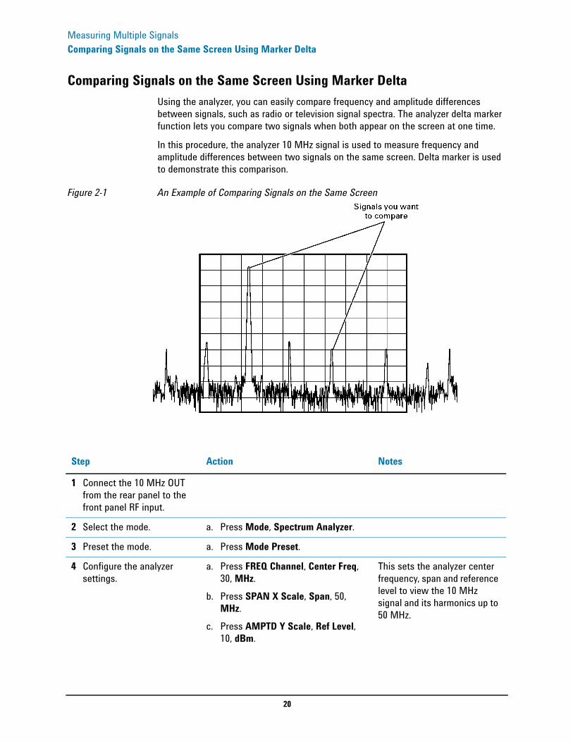
Comparing Signals on the Same Screen Using Marker DeltaUsing the analyzer, you can easily compare frequency and amplitude differences between signals, such as radio or television signal spectra. The analyzer delta marker function lets you compare two signals when both appear on the screen at one time.
In this procedure, the analyzer 10 MHz signal is used to measure frequency and amplitude differences between two signals on the same screen. Delta marker is used to demonstrate this comparison.
Figure 2-1 An Example of Comparing Signals on the Same Screen
Step Action Notes
1 Connect the 10 MHz OUT from the rear panel to the front panel RF input.
2 Select the mode. a. Press Mode, Spectrum Analyzer.
3 Preset the mode. a. Press Mode Preset.
4 Configure the analyzer settings.
a. Press FREQ Channel, Center Freq, 30, MHz.
b. Press SPAN X Scale, Span, 50, MHz.
c. Press AMPTD Y Scale, Ref Level, 10, dBm.
This sets the analyzer center frequency, span and reference level to view the 10 MHz signal and its harmonics up to 50 MHz.

21
Measuring Multiple SignalsComparing Signals on the Same Screen Using Marker Delta
5 Place a marker at the highest peak on the display (10 MHz).
a. Press Peak Search. The Next Pk Right and Next Pk Left softkeys are available to move the marker from peak to peak. The marker should be on the 10 MHz reference signal.
6 Anchor the first marker and activate a second delta marker.
a. Press Marker, Delta. The symbol for the first marker is changed from a diamond to a cross with a label that now reads 2, indicating that it is the fixed marker (reference point). The second marker symbol is a diamond labeled 1Δ2, indicating it is the delta marker. When you first press the Delta key, both markers are at the same frequency with the symbols superimposed over each other. It is not until you move the delta marker to a new frequency that the different marker symbols are easy to discern.
7 Move the delta marker to another signal peak.
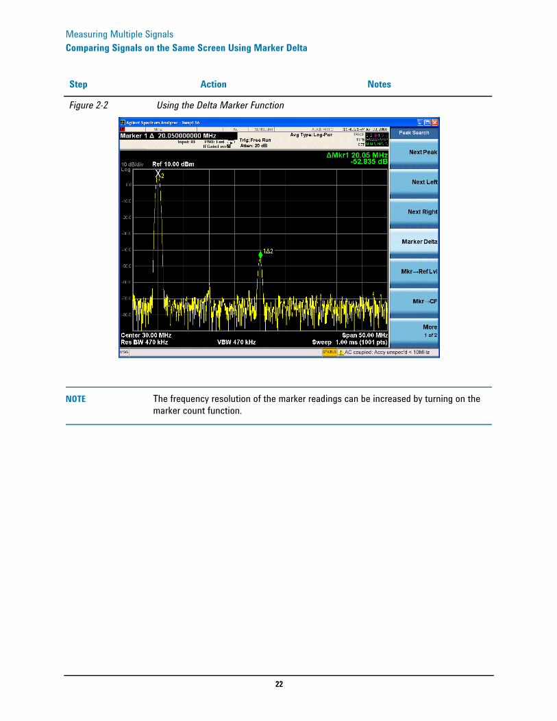
a. Press Peak Search, Next Peak. The amplitude and frequency difference between the markers is displayed in the marker results block of the screen. Refer to the upper right portion of the screen. See Figure 2-2.
Step Action Notes
22
Measuring Multiple SignalsComparing Signals on the Same Screen Using Marker Delta
NOTE The frequency resolution of the marker readings can be increased by turning on the marker count function.
Figure 2-2 Using the Delta Marker Function
Step Action Notes
23
Measuring Multiple SignalsComparing Signals not on the Same Screen Using Marker Delta
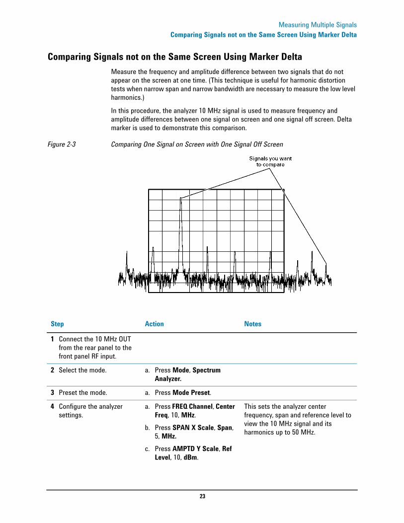
Comparing Signals not on the Same Screen Using Marker DeltaMeasure the frequency and amplitude difference between two signals that do not appear on the screen at one time. (This technique is useful for harmonic distortion tests when narrow span and narrow bandwidth are necessary to measure the low level harmonics.)
In this procedure, the analyzer 10 MHz signal is used to measure frequency and amplitude differences between one signal on screen and one signal off screen. Delta marker is used to demonstrate this comparison.
Figure 2-3 Comparing One Signal on Screen with One Signal Off Screen
Step Action Notes
1 Connect the 10 MHz OUT from the rear panel to the front panel RF input.
2 Select the mode. a. Press Mode, Spectrum Analyzer.
3 Preset the mode. a. Press Mode Preset.
4 Configure the analyzer settings.
a. Press FREQ Channel, Center Freq, 10, MHz.
b. Press SPAN X Scale, Span, 5, MHz.
c. Press AMPTD Y Scale, Ref Level, 10, dBm.
This sets the analyzer center frequency, span and reference level to view the 10 MHz signal and its harmonics up to 50 MHz.
24
Measuring Multiple SignalsComparing Signals not on the Same Screen Using Marker Delta
5 Place a marker at the highest peak on the display (10 MHz).
a. Press Peak Search.
6 Set the center frequency step size equal to the marker frequency.
a. Press Marker →, Mkr → CF Step.
7 Activate the marker delta function.
.
8 Increase the center frequency by 10 MHz.
a. Press FREQ Channel, Center Freq, ↑.
The first marker and delta markers move to the left edge of the screen, at the amplitude of the first signal peak.
9 Move the delta marker to the new center frequency.
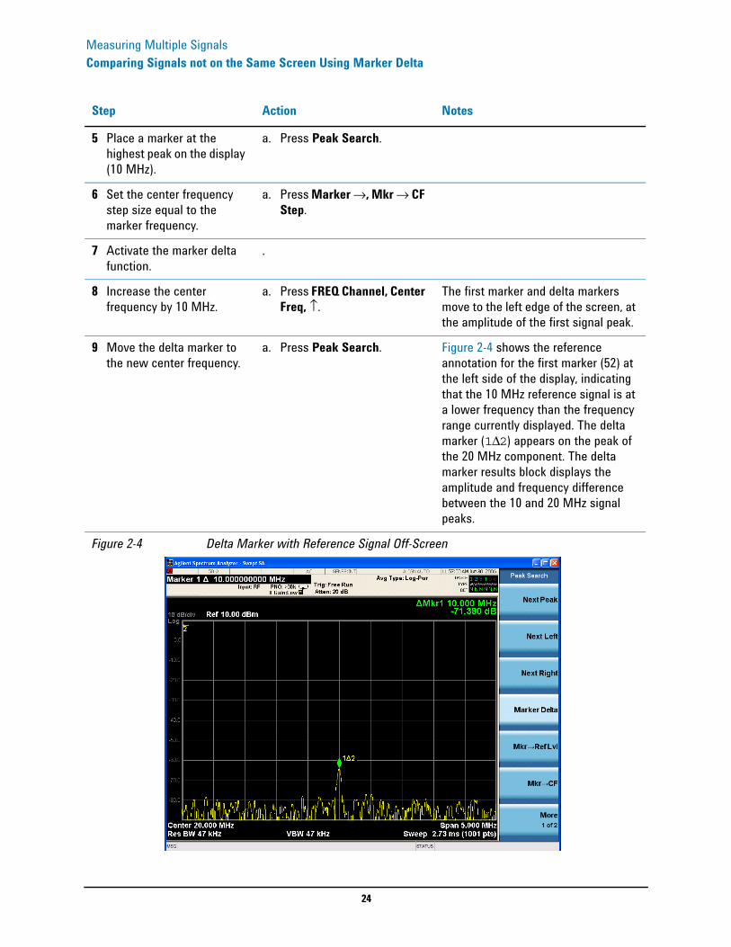
a. Press Peak Search. Figure 2-4 shows the reference annotation for the first marker (52) at the left side of the display, indicating that the 10 MHz reference signal is at a lower frequency than the frequency range currently displayed. The delta marker (1Δ2) appears on the peak of the 20 MHz component. The delta marker results block displays the amplitude and frequency difference between the 10 and 20 MHz signal peaks.
Figure 2-4 Delta Marker with Reference Signal Off-Screen
Step Action Notes
25
Measuring Multiple SignalsComparing Signals not on the Same Screen Using Marker Delta
10 Turn the markers off. Press Marker, Off.
Step Action Notes

26
Measuring Multiple SignalsResolving Signals of Equal Amplitude
Resolving Signals of Equal AmplitudeIn this procedure a decrease in resolution bandwidth is used in combination with a decrease in video bandwidth to resolve two signals of equal amplitude with a frequency separation of 100 kHz. Notice that the final RBW selection to resolve the signals is the same width as the signal separation while the VBW is slightly narrower than the RBW.
Step Action Notes
1 Connect two sources to the analyzer RF INPUT as shown.
2 Set up the signal sources. a. Set the frequency of signal generator #1 to 300 MHz.
b. Set the frequency of signal generator #2 to 300.1 MHz.
c. Set signal generator #1 amplitude to −20 dBm.
d. Set signal generator #2 amplitude to −4 dBm.
The amplitude of both signals should be approximately −20 dBm at the output of the bridge/directional coupler. (The −4 dBm setting plus −16 dB coupling factor of the 86205A results in a −20 dBm signal.)
3 Select the mode. a. Press Mode, Spectrum Analyzer.
4 Preset the analyzer. a. Press Mode Preset.
5 Set up the analyzer to view the signals.
a. Press FREQ Channel, Center Freq, 300, MHz.
b. Press BW, Res BW, 300, kHz.c. Press SPAN X Scale, Span, 2,
MHz..
A single signal peak is visible. See Figure 2-5.
27
Measuring Multiple SignalsResolving Signals of Equal Amplitude
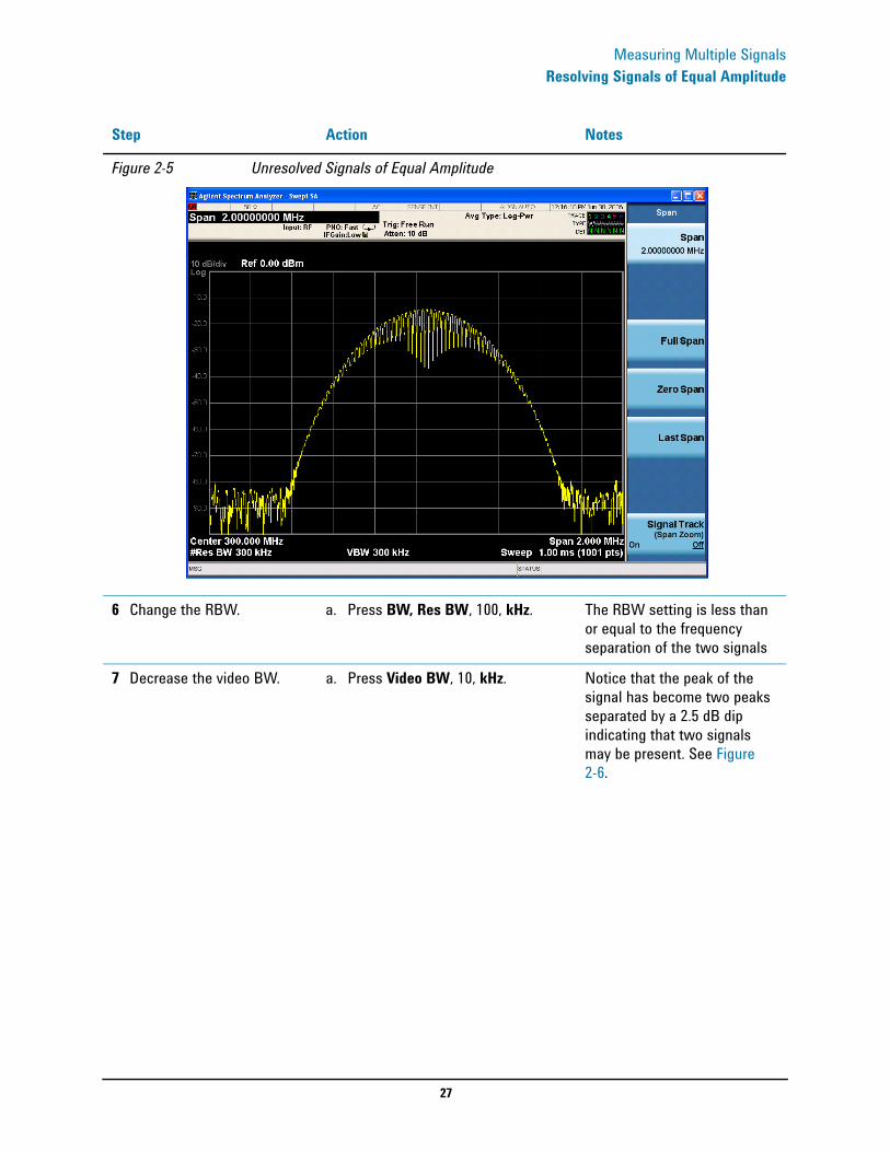
Figure 2-5 Unresolved Signals of Equal Amplitude
6 Change the RBW. a. Press BW, Res BW, 100, kHz. The RBW setting is less than or equal to the frequency separation of the two signals
7 Decrease the video BW. a. Press Video BW, 10, kHz. Notice that the peak of the signal has become two peaks separated by a 2.5 dB dip indicating that two signals may be present. See Figure 2-6.
Step Action Notes
28
Measuring Multiple SignalsResolving Signals of Equal Amplitude
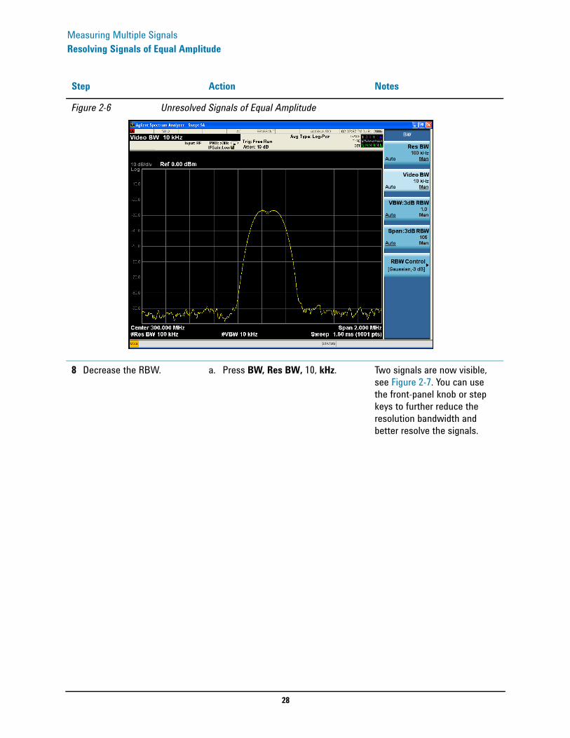
Figure 2-6 Unresolved Signals of Equal Amplitude
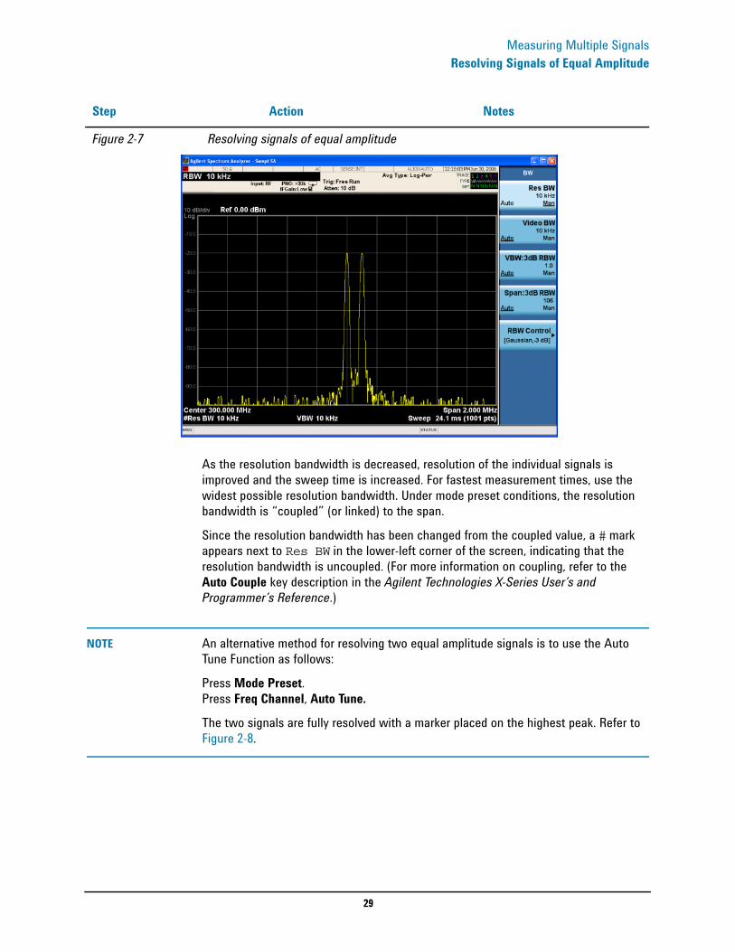
8 Decrease the RBW. a. Press BW, Res BW, 10, kHz. Two signals are now visible, see Figure 2-7. You can use the front-panel knob or step keys to further reduce the resolution bandwidth and better resolve the signals.
Step Action Notes
29
Measuring Multiple SignalsResolving Signals of Equal Amplitude
As the resolution bandwidth is decreased, resolution of the individual signals is improved and the sweep time is increased. For fastest measurement times, use the widest possible resolution bandwidth. Under mode preset conditions, the resolution bandwidth is “coupled” (or linked) to the span.
Since the resolution bandwidth has been changed from the coupled value, a # mark appears next to Res BW in the lower-left corner of the screen, indicating that the resolution bandwidth is uncoupled. (For more information on coupling, refer to the Auto Couple key description in the Agilent Technologies X-Series User’s and Programmer’s Reference.)
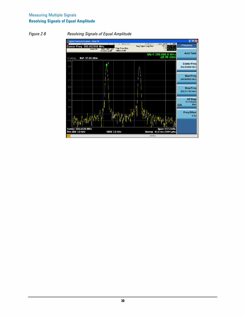
NOTE An alternative method for resolving two equal amplitude signals is to use the Auto Tune Function as follows:
Press Mode Preset. Press Freq Channel, Auto Tune.
The two signals are fully resolved with a marker placed on the highest peak. Refer to Figure 2-8.
Figure 2-7 Resolving signals of equal amplitude
Step Action Notes
30
Measuring Multiple SignalsResolving Signals of Equal Amplitude
Figure 2-8 Resolving Signals of Equal Amplitude
31
Measuring Multiple SignalsResolving Small Signals Hidden by Large Signals
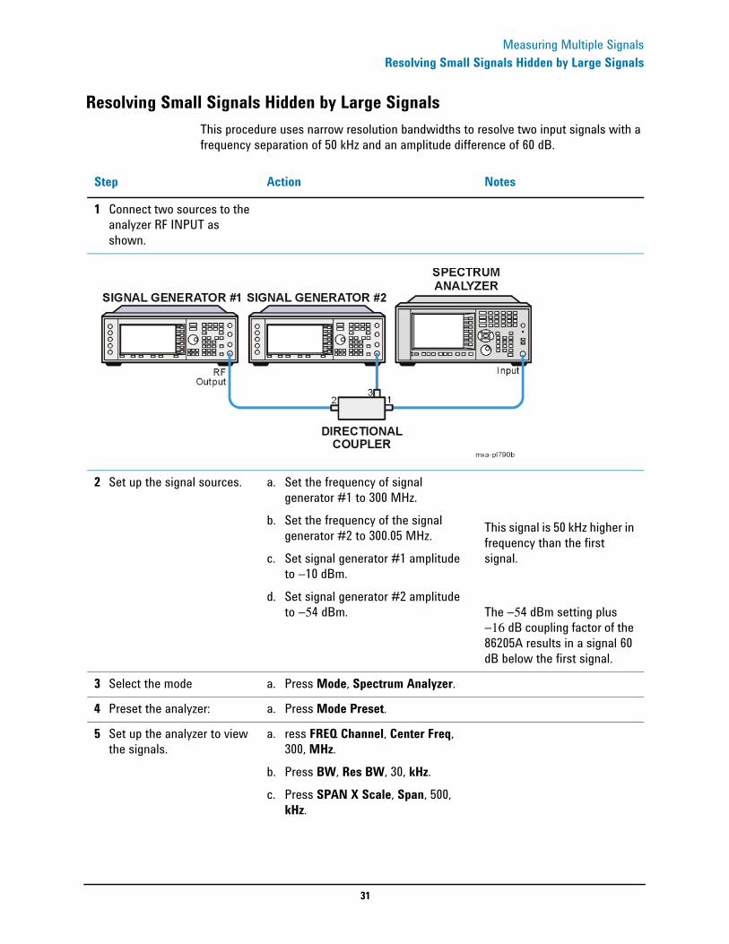
Resolving Small Signals Hidden by Large SignalsThis procedure uses narrow resolution bandwidths to resolve two input signals with a frequency separation of 50 kHz and an amplitude difference of 60 dB.
Step Action Notes
1 Connect two sources to the analyzer RF INPUT as shown.
2 Set up the signal sources. a. Set the frequency of signal generator #1 to 300 MHz.
b. Set the frequency of the signal generator #2 to 300.05 MHz.
c. Set signal generator #1 amplitude to −10 dBm.
d. Set signal generator #2 amplitude to −54 dBm.
This signal is 50 kHz higher in frequency than the first signal. The −54 dBm setting plus −16 dB coupling factor of the 86205A results in a signal 60 dB below the first signal.
3 Select the mode a. Press Mode, Spectrum Analyzer.
4 Preset the analyzer: a. Press Mode Preset.
5 Set up the analyzer to view the signals.
a. ress FREQ Channel, Center Freq, 300, MHz.
b. Press BW, Res BW, 30, kHz.c. Press SPAN X Scale, Span, 500,
kHz.
32
Measuring Multiple SignalsResolving Small Signals Hidden by Large Signals
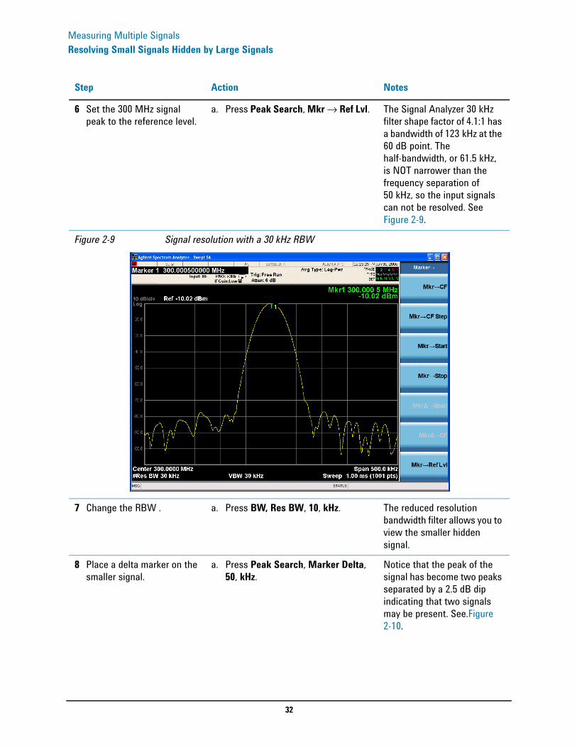
6 Set the 300 MHz signal peak to the reference level.
a. Press Peak Search, Mkr → Ref Lvl. The Signal Analyzer 30 kHz filter shape factor of 4.1:1 has a bandwidth of 123 kHz at the 60 dB point. The half-bandwidth, or 61.5 kHz, is NOT narrower than the frequency separation of 50 kHz, so the input signals can not be resolved. See Figure 2-9.
Figure 2-9 Signal resolution with a 30 kHz RBW
7 Change the RBW . a. Press BW, Res BW, 10, kHz. The reduced resolution bandwidth filter allows you to view the smaller hidden signal.
8 Place a delta marker on the smaller signal.
a. Press Peak Search, Marker Delta, 50, kHz.
Notice that the peak of the signal has become two peaks separated by a 2.5 dB dip indicating that two signals may be present. See.Figure 2-10.
Step Action Notes

33
Measuring Multiple SignalsResolving Small Signals Hidden by Large Signals
Figure 2-10 Unresolved Signals of Equal Amplitude
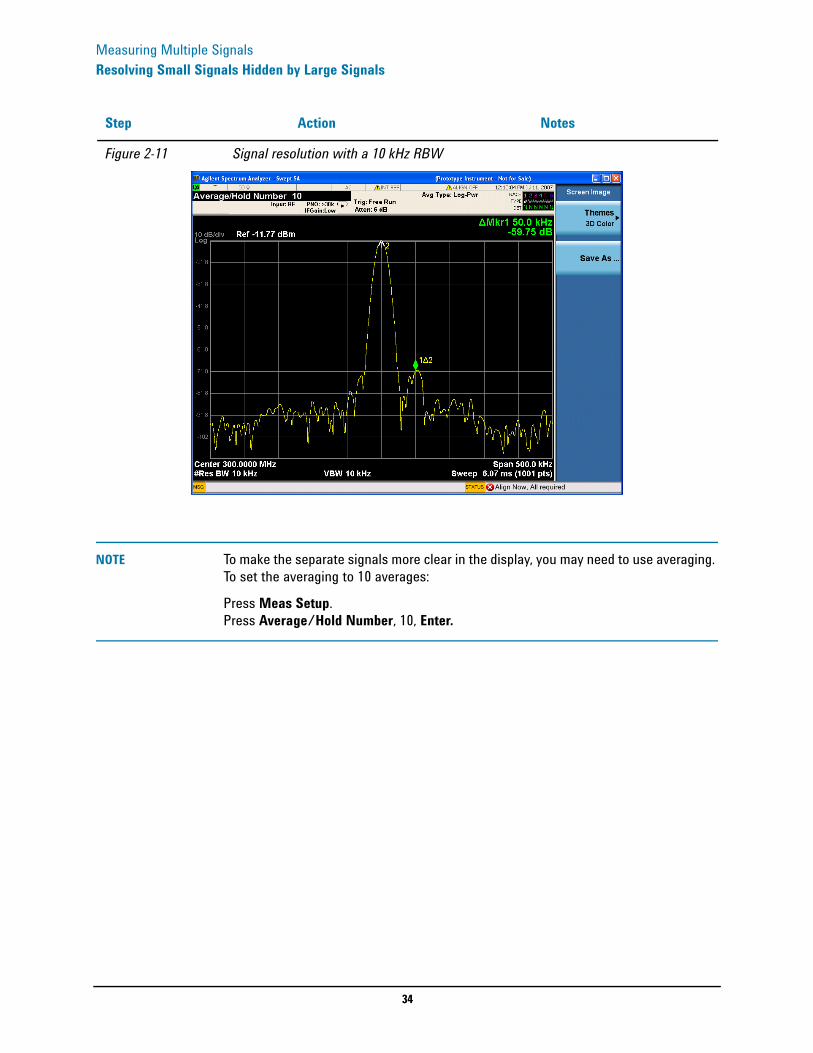
9 Decrease the RBW. a. Press BW, 10, kHz. The Signal Analyzer 10 kHz filter shape factor of 4.1:1 has a bandwidth of 4.1 kHz at the 60 dB point. The half-bandwidth, or 20.5 kHz, is narrower than 50 kHz, so the input signals can be resolved. See Figure 2-11.
Step Action Notes
34
Measuring Multiple SignalsResolving Small Signals Hidden by Large Signals
NOTE To make the separate signals more clear in the display, you may need to use averaging. To set the averaging to 10 averages:
Press Meas Setup. Press Average/Hold Number, 10, Enter.
Figure 2-11 Signal resolution with a 10 kHz RBW
Step Action Notes
35
Measuring Multiple SignalsDecreasing the Frequency Span Around the Signal
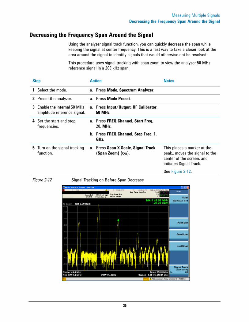
Decreasing the Frequency Span Around the SignalUsing the analyzer signal track function, you can quickly decrease the span while keeping the signal at center frequency. This is a fast way to take a closer look at the area around the signal to identify signals that would otherwise not be resolved.
This procedure uses signal tracking with span zoom to view the analyzer 50 MHz reference signal in a 200 kHz span.
Step Action Notes
1 Select the mode. a. Press Mode, Spectrum Analyzer.
2 Preset the analyzer. a. Press Mode Preset.
3 Enable the internal 50 MHz amplitude reference signal.
a. Press Input/Output, RF Calibrator, 50 MHz.
4 Set the start and stop frequencies.
a. Press FREQ Channel, Start Freq, 20, MHz.
b. Press FREQ Channel, Stop Freq, 1, GHz.
5 Turn on the signal tracking function.
a. Press Span X Scale, Signal Track (Span Zoom) (On).
This places a marker at the peak,. moves the signal to the center of the screen. and initiates Signal Track.See Figure 2-12.
Figure 2-12 Signal Tracking on Before Span Decrease

36
Measuring Multiple SignalsDecreasing the Frequency Span Around the Signal
6 Set the calibration signal to the reference level.
a. Press Mkr →, Mkr →Ref Lvl. Because the signal track function automatically maintains the signal at the center of the screen, you can reduce the span quickly for a closer look. If the signal drifts off of the screen as you decrease the span, use a wider frequency span.
7 Reduce the span and resolution bandwidth.
a. Press SPAN X Scale, Span, 200, kHz.
If the span change is large enough, the span decreases in steps as automatic zoom is completed. You can also use the front-panel knob or step keys to decrease the span and resolution bandwidth values.See Figure 2-13.
Figure 2-13 Signal Tracking After Zooming inon the Signal
8 Turn Signal tracking off. a. Press SPAN X Scale, Signal Track (Off).
Step Action Notes

37
Measuring Multiple SignalsEasily Measure Varying Levels of Modulated Power Compared to a Reference
Easily Measure Varying Levels of Modulated Power Compared to a ReferenceThis section demonstrates a method to measure the complex modulated power of a reference device or setup and then compare the result of adjustments and changes to that or other devices.
The Delta Band/Interval Power Marker function will be used to capture the simulated signal power of a reference device or setup and then compare the resulting power level due to adjustments or DUT changes.
An important key to making accurate Band Power Marker measurements is to insure that the Average Type under the Meas Setup key is set to “Auto”.
Step Action Notes
1 Connect the source RF OUTPUTto the analyzer RF INPUT as shown.
2 Set up the signal sources. a. Set up a 4-carrier W-CDMA signal.b. Set the source frequency to 1.96
GHz.c. Set the source amplitude to
−10 dBm.
3 Select the mode. a. Press Mode, Spectrum Analyzer.
4 Preset the analyzer. a. Press Mode Preset.
5 Tune to W-CDMA signal. a. Press FREQ Channel, Auto Tune, 300, MHz.
6 Set the analyzer reference level.
a. Press AMPTD Y Scale, Ref Level, 0, dBm.
7 Enable trace averaging. a. Press Trace/Detector, Select Trace, Trace 1, Trace Average.

38
Measuring Multiple SignalsEasily Measure Varying Levels of Modulated Power Compared to a Reference
8 Enable the Band/Interval Power Marker function.
a. Press Marker Function, Band/Interval Power.
This measures the total power of the reference 4-carrier W-CDMA signal
9 Center the frequency of the Band/Interval Power marker.
a. Press Select Marker, Marker 1, 1.96, GHz.
This centers the marker on the 4-carrier reference signal envelope.
10 Adjust the width (or span) of the Band/Interval Power marker.
a. Press Marker Function, Band Adjust, Band/Interval Span, 20, MHz.
This encompasses the entire 4-carrier W-CDMA reference signal. See Figure 2-14.Note the green vertical lines of Marker 1 representing the span of signals included in the Band/Interval Power measurement and the carrier power indicated in Markers Result Block.
Figure 2-14 Measured Power of Reference 4-carrier W-CDMA Signal Using Band/Interval Power Marker
Step Action Notes
39
Measuring Multiple SignalsEasily Measure Varying Levels of Modulated Power Compared to a Reference
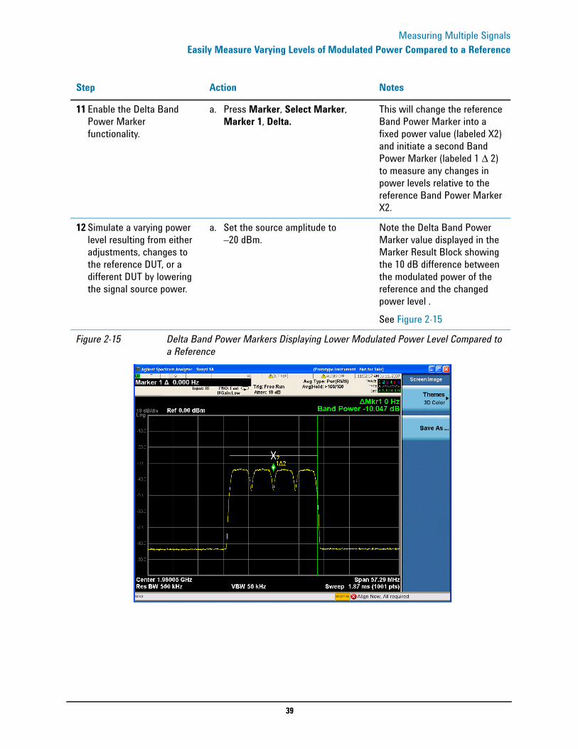
11 Enable the Delta Band Power Marker functionality.
a. Press Marker, Select Marker, Marker 1, Delta.
This will change the reference Band Power Marker into a fixed power value (labeled X2) and initiate a second Band Power Marker (labeled 1 Δ 2) to measure any changes in power levels relative to the reference Band Power Marker X2.
12 Simulate a varying power level resulting from either adjustments, changes to the reference DUT, or a different DUT by lowering the signal source power.
a. Set the source amplitude to –20 dBm.
Note the Delta Band Power Marker value displayed in the Marker Result Block showing the 10 dB difference between the modulated power of the reference and the changed power level .See Figure 2-15
Figure 2-15 Delta Band Power Markers Displaying Lower Modulated Power Level Compared to a Reference
Step Action Notes
40
Measuring Multiple SignalsEasily Measure Varying Levels of Modulated Power Compared to a Reference

41
Measuring a Low−Level Signal
3 Measuring a Low−Level Signal
42
Measuring a Low−Level SignalReducing Input Attenuation
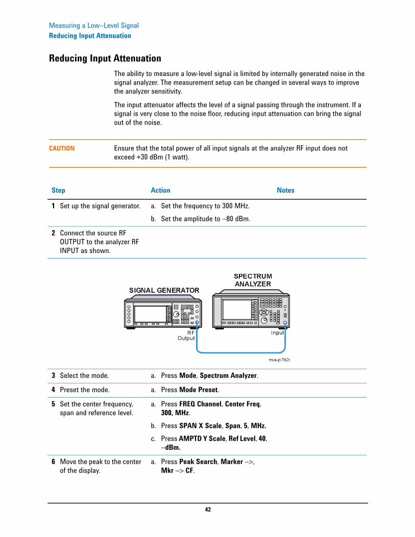
Reducing Input AttenuationThe ability to measure a low-level signal is limited by internally generated noise in the signal analyzer. The measurement setup can be changed in several ways to improve the analyzer sensitivity.
The input attenuator affects the level of a signal passing through the instrument. If a signal is very close to the noise floor, reducing input attenuation can bring the signal out of the noise.
CAUTION Ensure that the total power of all input signals at the analyzer RF input does not exceed +30 dBm (1 watt).
Step Action Notes
1 Set up the signal generator. a. Set the frequency to 300 MHz.b. Set the amplitude to −80 dBm.
2 Connect the source RF OUTPUT to the analyzer RF INPUT as shown.
3 Select the mode. a. Press Mode, Spectrum Analyzer.
4 Preset the mode. a. Press Mode Preset.
5 Set the center frequency, span and reference level.
a. Press FREQ Channel, Center Freq, 300, MHz.
b. Press SPAN X Scale, Span, 5, MHz.c. Press AMPTD Y Scale, Ref Level, 40,
−dBm.
6 Move the peak to the center of the display.
a. Press Peak Search, Marker −>, Mkr −> CF.
43
Measuring a Low−Level SignalReducing Input Attenuation
7 Reduce the span. a. Press Span, 1, MHz. If necessary re-center the peak.
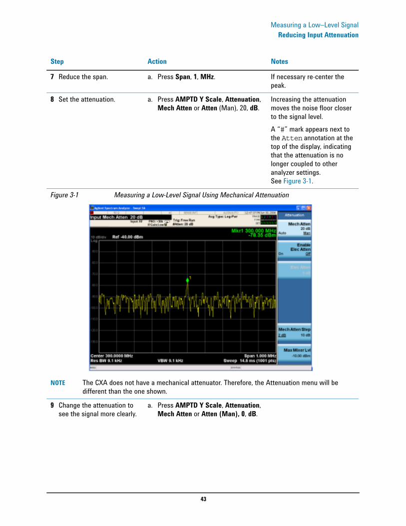
8 Set the attenuation. a. Press AMPTD Y Scale, Attenuation, Mech Atten or Atten (Man), 20, dB.
Increasing the attenuation moves the noise floor closer to the signal level. A “#” mark appears next to the Atten annotation at the top of the display, indicating that the attenuation is no longer coupled to other analyzer settings. See Figure 3-1.
Figure 3-1 Measuring a Low-Level Signal Using Mechanical Attenuation
NOTE The CXA does not have a mechanical attenuator. Therefore, the Attenuation menu will be different than the one shown.
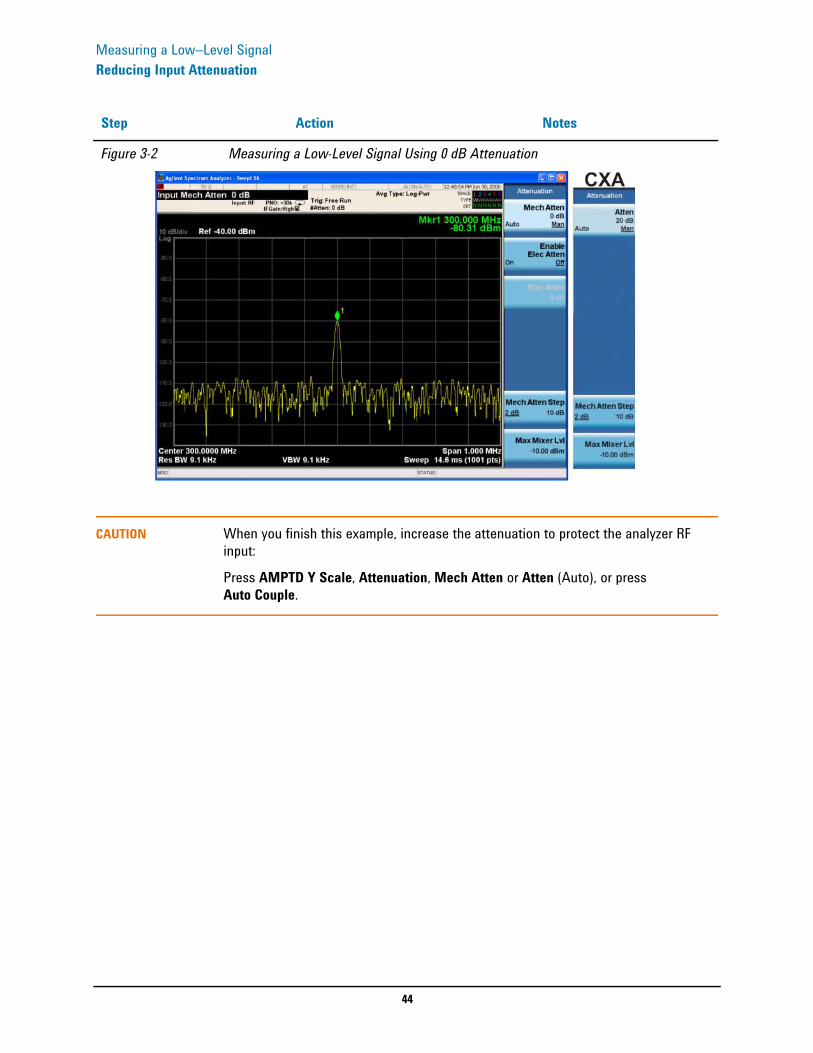
9 Change the attenuation to see the signal more clearly.
a. Press AMPTD Y Scale, Attenuation, Mech Atten or Atten (Man), 0, dB.
Step Action Notes
44
Measuring a Low−Level SignalReducing Input Attenuation
CAUTION When you finish this example, increase the attenuation to protect the analyzer RF input:
Press AMPTD Y Scale, Attenuation, Mech Atten or Atten (Auto), or press Auto Couple.
Figure 3-2 Measuring a Low-Level Signal Using 0 dB Attenuation
Step Action Notes
45
Measuring a Low−Level SignalDecreasing the Resolution Bandwidth
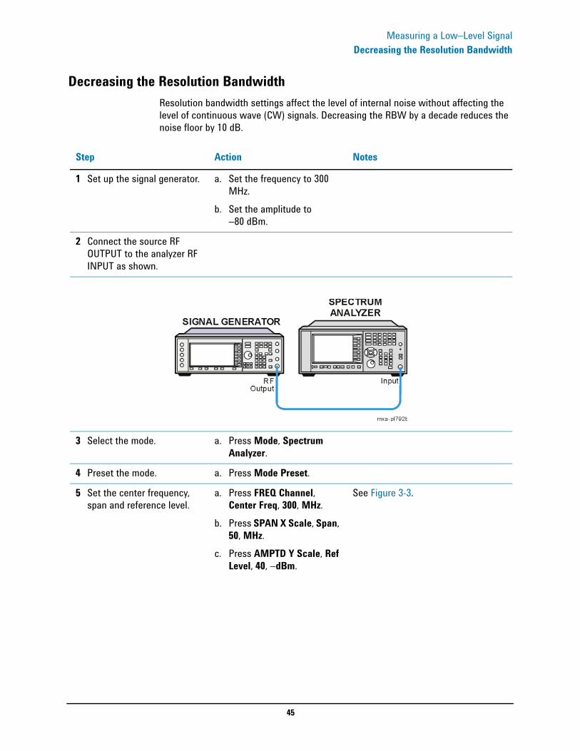
Decreasing the Resolution BandwidthResolution bandwidth settings affect the level of internal noise without affecting the level of continuous wave (CW) signals. Decreasing the RBW by a decade reduces the noise floor by 10 dB.
Step Action Notes
1 Set up the signal generator. a. Set the frequency to 300 MHz.
b. Set the amplitude to −80 dBm.
2 Connect the source RF OUTPUT to the analyzer RF INPUT as shown.
3 Select the mode. a. Press Mode, Spectrum Analyzer.
4 Preset the mode. a. Press Mode Preset.
5 Set the center frequency, span and reference level.
a. Press FREQ Channel, Center Freq, 300, MHz.
b. Press SPAN X Scale, Span, 50, MHz.
c. Press AMPTD Y Scale, Ref Level, 40, −dBm.
See Figure 3-3.

46
Measuring a Low−Level SignalDecreasing the Resolution Bandwidth
Figure 3-3 Default resolution bandwidth
6 Decrease the RBW. a. Press BW, 47, kHz. The low-level signal appears more clearly because the noise level is reduced. See Figure 3-4.
Figure 3-4 Decreasing Resolution Bandwidth
A “#” mark appears next to the Res BW annotation in the lower left corner of the screen, indicating that the resolution bandwidth is uncoupled.
Step Action Notes
47
Measuring a Low−Level SignalDecreasing the Resolution Bandwidth
RBW Selections You can use the step keys to change the RBW in a 1−3−10 sequence.
All the Signal Analyzer RBWs are digital and have a selectivity ratio of 4.1:1. Choosing the next lower RBW (in a 1−3−10 sequence) for better sensitivity increases the sweep time by about 10:1 for swept measurements, and about 3:1 for FFT measurements (within the limits of RBW). Using the knob or keypad, you can select RBWs from 1 Hz to 3 MHz in approximately 10% increments, plus 4, 5, 6 and 8 MHz. This enables you to make the trade off between sweep time and sensitivity with finer resolution.
48
Measuring a Low−Level SignalUsing the Average Detector and Increased Sweep Time
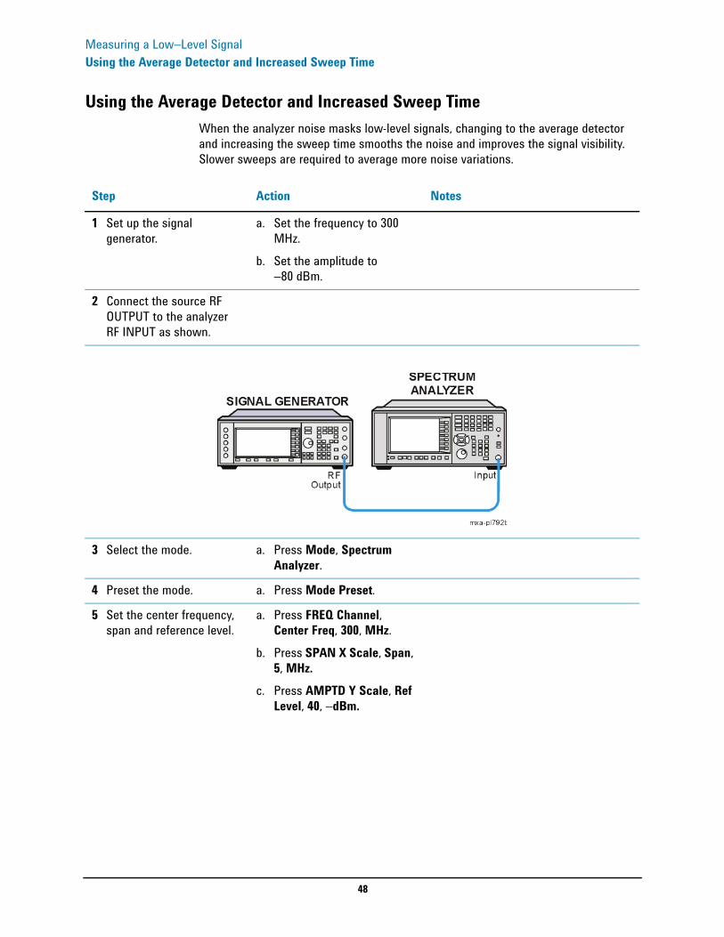
Using the Average Detector and Increased Sweep TimeWhen the analyzer noise masks low-level signals, changing to the average detector and increasing the sweep time smooths the noise and improves the signal visibility. Slower sweeps are required to average more noise variations.
Step Action Notes
1 Set up the signal generator.
a. Set the frequency to 300 MHz.
b. Set the amplitude to −80 dBm.
2 Connect the source RF OUTPUT to the analyzer RF INPUT as shown.
3 Select the mode. a. Press Mode, Spectrum Analyzer.
4 Preset the mode. a. Press Mode Preset.
5 Set the center frequency, span and reference level.
a. Press FREQ Channel, Center Freq, 300, MHz.
b. Press SPAN X Scale, Span, 5, MHz.
c. Press AMPTD Y Scale, Ref Level, 40, −dBm.
49
Measuring a Low−Level SignalUsing the Average Detector and Increased Sweep Time
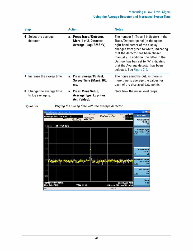
6 Select the average detector.
a. Press Trace/Detector, More 1 of 2, Detector, Average (Log/RMS/V).
The number 1 (Trace 1 indicator) in the Trace/Detector panel (in the upper right-hand corner of the display) changes from green to white, indicating that the detector has been chosen manually. In addition, the letter in the Det row has ben set to “A” indicating that the Average detector has been selected. See Figure 3-5.
7 Increase the sweep time. a. Press Sweep/Control, Sweep Time (Man), 100, ms.
The noise smooths out, as there is more time to average the values for each of the displayed data points.
8 Change the average type to log averaging.
a. Press Meas Setup, Average Type, Log-Pwr Avg (Video).
Note how the noise level drops.
Figure 3-5 Varying the sweep time with the average detector
Step Action Notes
50
Measuring a Low−Level SignalTrace Averaging
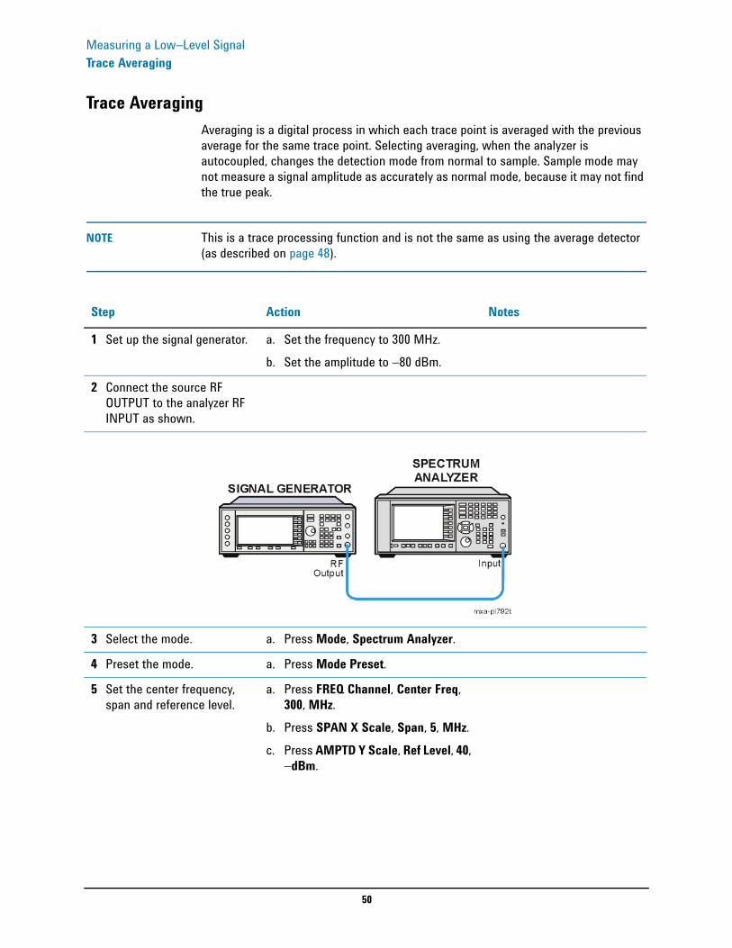
Trace AveragingAveraging is a digital process in which each trace point is averaged with the previous average for the same trace point. Selecting averaging, when the analyzer is autocoupled, changes the detection mode from normal to sample. Sample mode may not measure a signal amplitude as accurately as normal mode, because it may not find the true peak.
NOTE This is a trace processing function and is not the same as using the average detector (as described on page 48).
Step Action Notes
1 Set up the signal generator. a. Set the frequency to 300 MHz.b. Set the amplitude to −80 dBm.
2 Connect the source RF OUTPUT to the analyzer RF INPUT as shown.
3 Select the mode. a. Press Mode, Spectrum Analyzer.
4 Preset the mode. a. Press Mode Preset.
5 Set the center frequency, span and reference level.
a. Press FREQ Channel, Center Freq, 300, MHz.
b. Press SPAN X Scale, Span, 5, MHz.c. Press AMPTD Y Scale, Ref Level, 40,
−dBm.

51
Measuring a Low−Level SignalTrace Averaging
Changing most active functions restarts the averaging, as does pressing the Restart key. Once the set number of sweeps completes, the analyzer continues to provide a running average based on this set number.
NOTE If you want the measurement to stop after the set number of sweeps, use single sweep: Press Single and then press the Restart key.
6 Turn on Averaging. a. Press Trace/Detector, Trace Average.
As the averaging routine smooths the trace, low level signals become more visible. Avg/Hold >100 appears in the measurement bar near the top of the screen. SeeFigure 3-6.
7 Set number of averages. a. Press Meas Setup, Average/Hold Number, 25, Enter.
Annotation above the graticule in the measurement bar to the right of center shows the type of averaging, Log-Power. Also, the number of traces averaged is shown on the Average/Hold Number key.
Figure 3-6 Trace Averaging
Step Action Notes

52
Measuring a Low−Level SignalTrace Averaging
53
Improving Frequency Resolution and Accuracy
4 Improving Frequency Resolution and Accuracy
54
Improving Frequency Resolution and AccuracyUsing a Frequency Counter to Improve Frequency Resolution and Accuracy
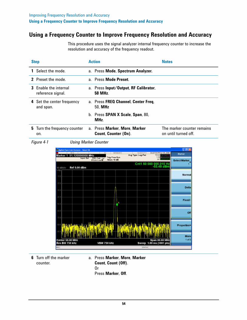
Using a Frequency Counter to Improve Frequency Resolution and AccuracyThis procedure uses the signal analyzer internal frequency counter to increase the resolution and accuracy of the frequency readout.
Step Action Notes
1 Select the mode. a. Press Mode, Spectrum Analyzer.
2 Preset the mode. a. Press Mode Preset.
3 Enable the internal reference signal.
a. Press Input/Output, RF Calibrator, 50 MHz.
4 Set the center frequency and span.
a. Press FREQ Channel, Center Freq, 50, MHz
b. Press SPAN X Scale, Span, 80, MHz.
5 Turn the frequency counter on.
a. Press Marker, More, Marker Count, Counter (On).
The marker counter remains on until turned off.
Figure 4-1 Using Marker Counter
6 Turn off the marker counter.
a. Press Marker, More, Marker Count, Count (Off). Or Press Marker, Off.
55
Tracking Drifting Signals
5 Tracking Drifting Signals
56
Tracking Drifting SignalsMeasuring a Source Frequency Drift
Measuring a Source Frequency DriftThe analyzer can measure the short- and long-term stability of a source. The maximum amplitude level and the frequency drift of an input signal trace can be displayed and held by using the maximum-hold function. You can also use the maximum hold function if you want to determine how much of the frequency spectrum a signal occupies.
This procedure using signal tracking to keep the drifting signal in the center of the display. The drifting is captured by the analyzer using maximum hold.
Step Action Notes
1 Setup the signal sources. a. Set the frequency of the signal source to 300 MHz.
b. Set the source amplitude to −20 dBm
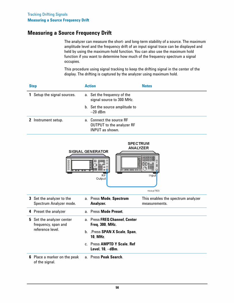
2 Instrument setup. a. Connect the source RF OUTPUT to the analyzer RF INPUT as shown.
3 Set the analyzer to the Spectrum Analyzer mode.
a. Press Mode, Spectrum Analyzer.
This enables the spectrum analyzer measurements.
4 Preset the analyzer a. Press Mode Preset.
5 Set the analyzer center frequency, span and reference level.
a. Press FREQ Channel, Center Freq, 300, MHz.
b. .Press SPAN X Scale, Span, 10, MHz.
c. Press AMPTD Y Scale, Ref Level, 10, −dBm.
6 Place a marker on the peak of the signal.
a. Press Peak Search.

57
Tracking Drifting SignalsMeasuring a Source Frequency Drift
7 Turn on the signal tracking function.
a. Press SPAN X Scale, Signal Track (On).
8 Reduce the span to 500 kHz. a. Press SPAN, 500, kHz. Notice that the signal is held in the center of the display.
9 Turn off the signal track function.
a. Press SPAN X Scale, Signal Track (Off).
10 Measure the excursion of the signal.
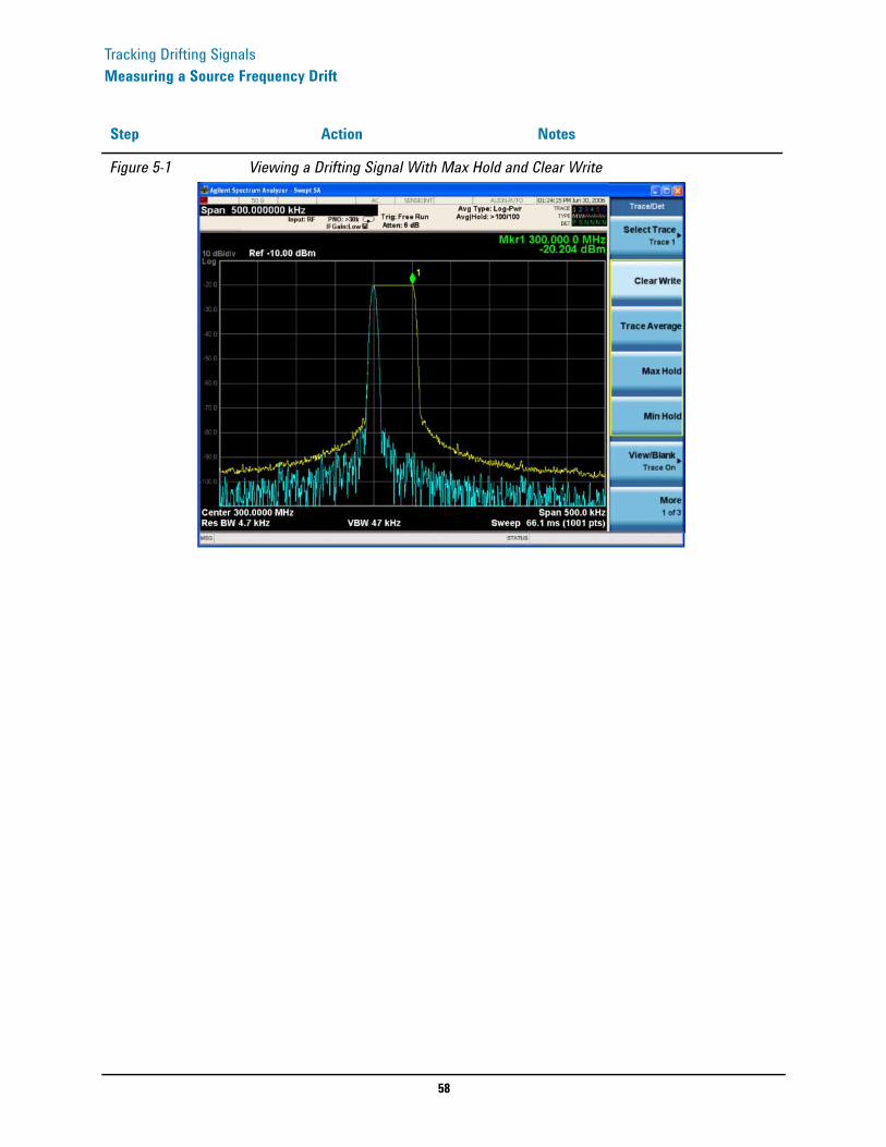
a. Press Trace/Detector, Max Hold.
As the signal varies, maximum hold maintains the maximum responses of the input signal.Annotation in the Trace/Detector panel, upper right corner of the screen, indicates the trace mode. In this example, the M in the Type row under TRACE 1 indicates trace 1 is in maximum-hold mode.
11 Activate trace 2. a. Press Trace/Detector, Select Trace, Trace (2).
Trace 1 remains in maximum hold mode to show any drift in the signal.
12 Change the mode to continuous sweeping.
a. Press Clear Write.
13 Slowly change the frequency of the signal generator ± 50 kHz in 1 kHz increments.
Your analyzer display should look similar to Figure 5-1.
Step Action Notes
58
Tracking Drifting SignalsMeasuring a Source Frequency Drift
Figure 5-1 Viewing a Drifting Signal With Max Hold and Clear Write
Step Action Notes
59
Tracking Drifting SignalsTracking a Signal
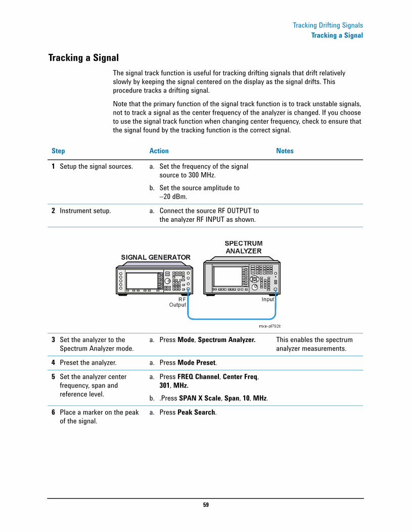
Tracking a SignalThe signal track function is useful for tracking drifting signals that drift relatively slowly by keeping the signal centered on the display as the signal drifts. This procedure tracks a drifting signal.
Note that the primary function of the signal track function is to track unstable signals, not to track a signal as the center frequency of the analyzer is changed. If you choose to use the signal track function when changing center frequency, check to ensure that the signal found by the tracking function is the correct signal.
Step Action Notes
1 Setup the signal sources. a. Set the frequency of the signal source to 300 MHz.
b. Set the source amplitude to −20 dBm.
2 Instrument setup. a. Connect the source RF OUTPUT to the analyzer RF INPUT as shown.
3 Set the analyzer to the Spectrum Analyzer mode.
a. Press Mode, Spectrum Analyzer. This enables the spectrum analyzer measurements.
4 Preset the analyzer. a. Press Mode Preset.
5 Set the analyzer center frequency, span and reference level.
a. Press FREQ Channel, Center Freq, 301, MHz.
b. .Press SPAN X Scale, Span, 10, MHz.
6 Place a marker on the peak of the signal.
a. Press Peak Search.
60
Tracking Drifting SignalsTracking a Signal
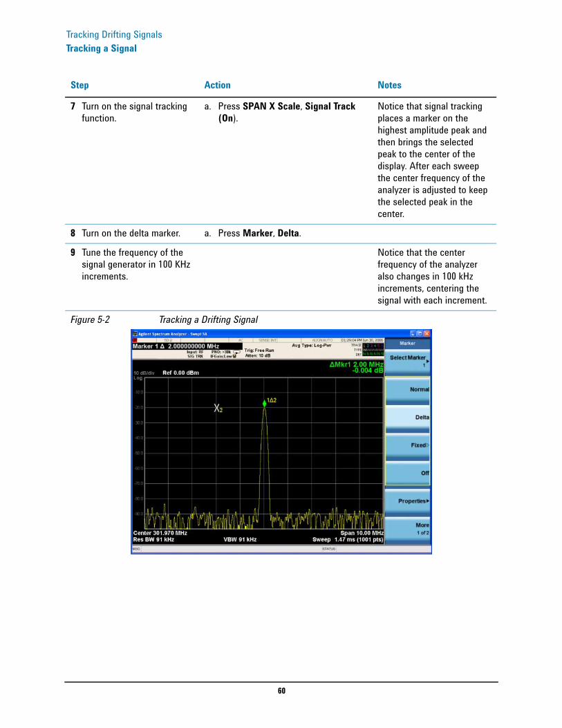
7 Turn on the signal tracking function.
a. Press SPAN X Scale, Signal Track (On).
Notice that signal tracking places a marker on the highest amplitude peak and then brings the selected peak to the center of the display. After each sweep the center frequency of the analyzer is adjusted to keep the selected peak in the center.
8 Turn on the delta marker. a. Press Marker, Delta.
9 Tune the frequency of the signal generator in 100 KHz increments.
Notice that the center frequency of the analyzer also changes in 100 kHz increments, centering the signal with each increment.
Figure 5-2 Tracking a Drifting Signal
Step Action Notes
61
Making Distortion Measurements
6 Making Distortion Measurements
62
Making Distortion MeasurementsIdentifying Analyzer Generated Distortion
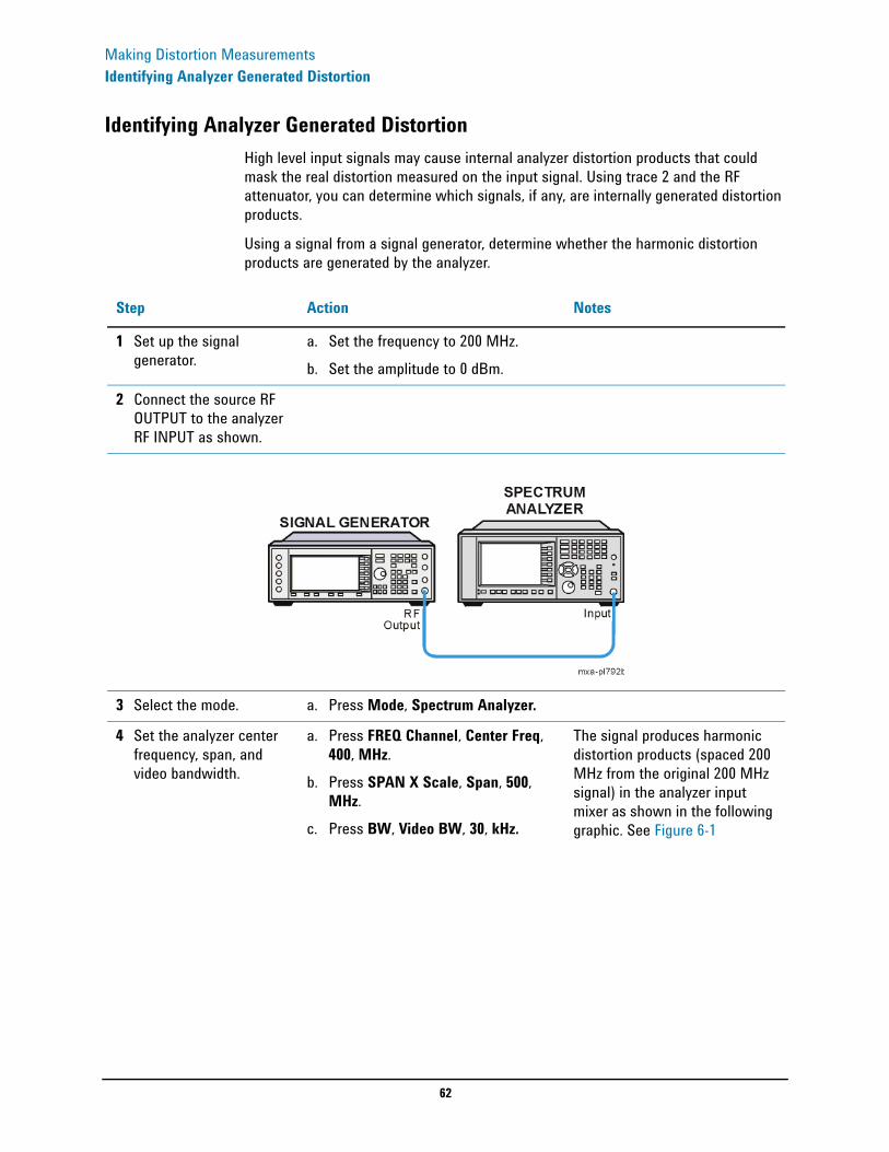
Identifying Analyzer Generated DistortionHigh level input signals may cause internal analyzer distortion products that could mask the real distortion measured on the input signal. Using trace 2 and the RF attenuator, you can determine which signals, if any, are internally generated distortion products.
Using a signal from a signal generator, determine whether the harmonic distortion products are generated by the analyzer.
Step Action Notes
1 Set up the signal generator.
a. Set the frequency to 200 MHz.b. Set the amplitude to 0 dBm.
2 Connect the source RF OUTPUT to the analyzer RF INPUT as shown.
3 Select the mode. a. Press Mode, Spectrum Analyzer.
4 Set the analyzer center frequency, span, and video bandwidth.
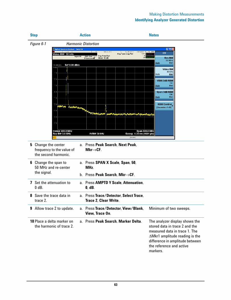
a. Press FREQ Channel, Center Freq, 400, MHz.
b. Press SPAN X Scale, Span, 500, MHz.
c. Press BW, Video BW, 30, kHz.
The signal produces harmonic distortion products (spaced 200 MHz from the original 200 MHz signal) in the analyzer input mixer as shown in the following graphic. See Figure 6-1
63
Making Distortion MeasurementsIdentifying Analyzer Generated Distortion
Figure 6-1 Harmonic Distortion
5 Change the center frequency to the value of the second harmonic.
a. Press Peak Search, Next Peak, Mkr→CF.
6 Change the span to 50 MHz and re-center the signal.
a. Press SPAN X Scale, Span, 50, MHz.
b. Press Peak Search, Mkr→CF.
7 Set the attenuation to 0 dB.
a. Press AMPTD Y Scale, Attenuation, 0, dB.
8 Save the trace data in trace 2.
a. Press Trace/Detector, Select Trace, Trace 2, Clear Write.
9 Allow trace 2 to update. a. Press Trace/Detector, View/Blank, View, Trace On.
Minimum of two sweeps.
10 Place a delta marker on the harmonic of trace 2.
a. Press Peak Search, Marker Delta. The analyzer display shows the stored data in trace 2 and the measured data in trace 1. The ΔMkr1 amplitude reading is the difference in amplitude between the reference and active markers.
Step Action Notes
64
Making Distortion MeasurementsIdentifying Analyzer Generated Distortion
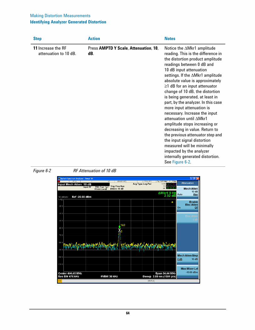
11 Increase the RF attenuation to 10 dB.
Press AMPTD Y Scale, Attenuation, 10, dB.
Notice the ΔMkr1 amplitude reading. This is the difference in the distortion product amplitude readings between 0 dB and 10 dB input attenuation settings. If the ΔMkr1 amplitude absolute value is approximately ≥1 dB for an input attenuator change of 10 dB, the distortion is being generated, at least in part, by the analyzer. In this case more input attenuation is necessary. Increase the input attenuation until ΔMkr1 amplitude stops increasing or decreasing in value. Return to the previous attenuator step and the input signal distortion measured will be minimally impacted by the analyzer internally generated distortion. See Figure 6-2.
Figure 6-2 RF Attenuation of 10 dB
Step Action Notes

65
Making Distortion MeasurementsThird-Order Intermodulation Distortion
Third-Order Intermodulation DistortionTwo-tone, third-order intermodulation distortion is a common test in communication systems. When two signals are present in a non-linear system, they can interact and create third-order intermodulation distortion products that are located close to the original signals. These distortion products are generated by system components such as amplifiers and mixers.
This procedure tests a device for third-order intermodulation using markers. Two sources are used, one set to 300 MHz and the other to 301 MHz. This combination of signal generators and a directional coupler (used as a combiner) results in a two-tone source with very low intermodulation distortion. Although the distortion from this setup may be better than the specified performance of the analyzer, it is useful for determining the TOI performance of the source/analyzer combination. After the performance of the source/analyzer combination has been verified, the device-under-test (DUT) (for example, an amplifier) would be inserted between the directional coupler output and the analyzer input.
Step Action Notes
1 Connect two sources to the analyzer RF INPUT as shown.
The coupler should have a high degree of isolation between the two input ports so the sources do not intermodulate.
2 Set up the signal sources. a. Set the frequency of signal generator #1 to 300 MHz.
b. Set the frequency of signal generator #2 to 300.1 MHz.
c. Set signal generator #1 amplitude to −5 dBm.
d. Set signal generator #2 amplitude to −5 dBm.
This produces a frequency separation of 1 MHz.Sets the sources equal in amplitude as measured by the analyzer.

66
Making Distortion MeasurementsThird-Order Intermodulation Distortion
3 Select the mode. a. Press Mode, Spectrum Analyzer.
4 Preset the analyzer. a. Press Mode Preset.
5 Set the analyzer center frequency and span.
a. Press FREQ Channel, Center Freq, 300.5, MHz.
b. Press SPAN X Scale, Span, 5, MHz
6 Set the analyzer detector to Peak.
a. Press Trace/Detector, Detector, Peak.
7 Set the mixer level to improve dynamic range.
a. Press AMPTD Y Scale, Attenuation, Max Mixer Lvl, –10, dBm.
The analyzer automatically sets the attenuation so that a signal at the reference level has a maximum value of −10 dBm at the input mixer.
8 Move the signal to the reference level.
a. Press Peak Search, Mkr →, Mkr → Ref Lvl.
9 Reduce the RBW until the distortion products are visible.
a. Press BW, Res BW, ↓.
10 Activate the second marker and place it on the peak of the distortion product closest to the marker test signal.
a. Press Peak Search, Marker Delta, Next Left or Next Right (as appropriate).
Use the Next Right key (if the first marker is on the right test signal) or Next Left key (if the first marker is on the left test signal):
11 Measure the other distortion product
a. Press Marker, Normal, Peak Search, Next Peak.
12 Activate the second marker and place it on the peak of the distortion product closest to the marked test signal.
Press Marker, Normal, Marker Delta, Next Left or Next Right (as appropriate).
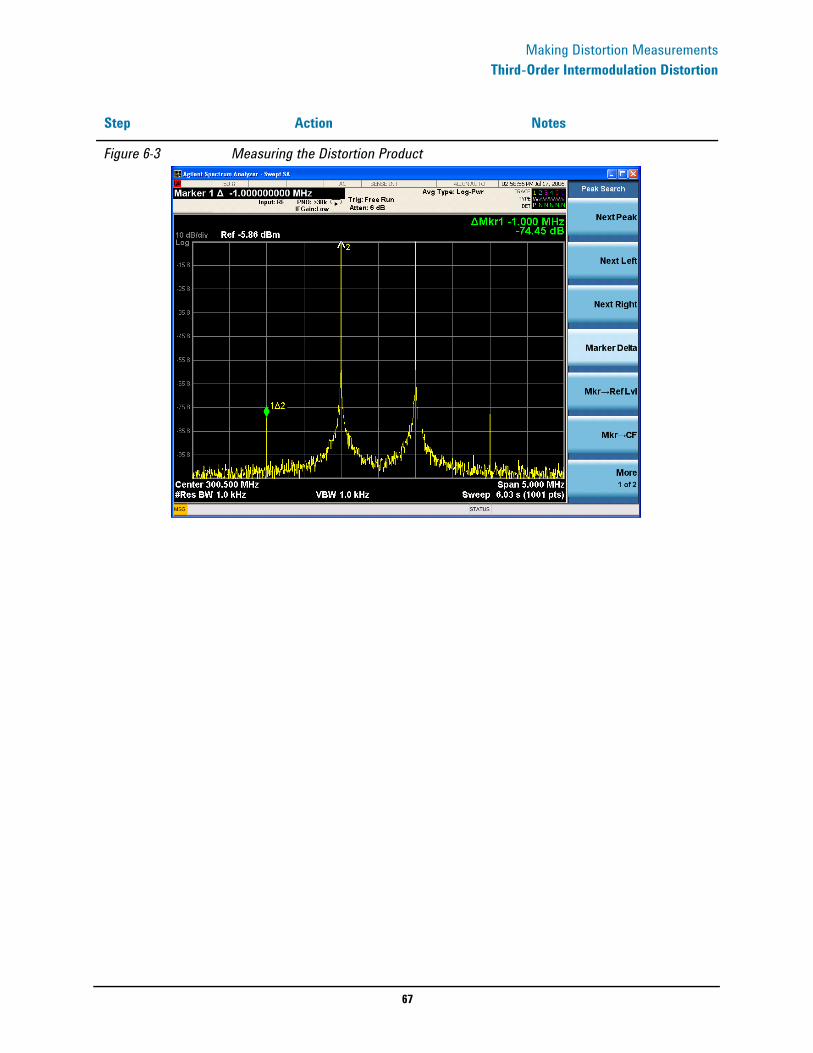
See Figure 6-3.
Step Action Notes
67
Making Distortion MeasurementsThird-Order Intermodulation Distortion
Figure 6-3 Measuring the Distortion Product
Step Action Notes
68
Making Distortion MeasurementsThird-Order Intermodulation Distortion
69
Measuring Noise
7 Measuring Noise

70
Measuring NoiseMeasuring Signal-to-Noise
Measuring Signal-to-Noise Signal-to-noise is a ratio used in many communication systems as an indication of noise in a system. Typically the more signals added to a system adds to the noise level, reducing the signal-to-noise ratio making it more difficult for modulated signals to be demodulated. This measurement is also referred to as carrier-to-noise in some communication systems.
The signal-to-noise measurement procedure below may be adapted to measure any signal in a system if the signal (carrier) is a discrete tone. If the signal in your system is modulated, it is necessary to modify the procedure to correctly measure the modulated signal level.
In this example the 50 MHz amplitude reference signal is used as the fundamental signal. The amplitude reference signal is assumed to be the signal of interest and the internal noise of the analyzer is measured as the system noise. To do this, you need to set the input attenuator such that both the signal and the noise are well within the calibrated region of the display.
Step Action Notes
1 Set the analyzer to the Spectrum Analyzer mode.
a. Press Mode, Spectrum Analyzer. This enables the spectrum analyzer measurements.
2 Preset the analyzer. a. Press Mode Preset.
3 Enable the internal reference signal.
a. Press Input/Output, RF Calibrator, 50, MHz.
4 Set the center frequency, span, reference level and attenuation.
a. Press FREQ Channel, Center Freq, 50, MHz.
b. Press SPAN X Scale, Span, 1, MHz.c. Press AMPTD Y Scale, Ref Level,
−10, dBm.d. Press AMPTD Y Scale, Attenuation,
40, dB.
5 Place a marker on the peak of the signal and place a delta marker in the noise.
a. Press Peak Search, Marker Delta, 200, kHz.
6 Turn on the marker noise function.
a. Press Marker Function, Marker Noise.
This enables you to view the signal-to-noise measurement results.
71
Measuring NoiseMeasuring Signal-to-Noise
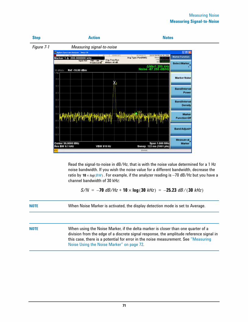
Read the signal-to-noise in dB/Hz, that is with the noise value determined for a 1 Hz noise bandwidth. If you wish the noise value for a different bandwidth, decrease the ratio by . For example, if the analyzer reading is −70 dB/Hz but you have a channel bandwidth of 30 kHz:
NOTE When Noise Marker is activated, the display detection mode is set to Average.
NOTE When using the Noise Marker, if the delta marker is closer than one quarter of a division from the edge of a discrete signal response, the amplitude reference signal in this case, there is a potential for error in the noise measurement. See “Measuring Noise Using the Noise Marker” on page 72.
Figure 7-1 Measuring signal-to-noise
Step Action Notes
10 log× BW( )
S/N 70– dB/Hz 10 30 kHz( )log×+ 25.23 dB– 30 kHz( )⁄= =

72
Measuring NoiseMeasuring Noise Using the Noise Marker
Measuring Noise Using the Noise MarkerThis procedure uses the marker function, Marker Noise, to measure noise in a 1 Hz bandwidth. In this example the noise marker measurement is made near the 50 MHz reference signal to illustrate the use of Marker Noise.
Step Action Notes
1 Set the analyzer to the Spectrum Analyzer mode.
a. Press Mode, Spectrum Analyzer.
This enables the spectrum analyzer measurements
2 Preset the analyzer. a. Press Mode Preset.
3 Enable the internal reference signal.
a. Press Input/Output, RF Calibrator, 50, MHz.
4 Set the center frequency, span, reference level and attenuation.
a. Press FREQ Channel, Center Freq, 49.98, MHz.
b. Press SPAN X Scale, Span, 100, kHz.
c. Press AMPTD Y Scale, Ref Level, −10, dBm.
d. Press AMPTD Y Scale, Attenuation, Mech Atten Man, 40, dB.
5 Turn on the noise marker. a. Press Marker Function, Marker Noise.
Note that display detection automatically changes to “Avg”; average detection calculates the noise marker from an average value of the displayed noise. Notice that the noise marker floats between the maximum and the minimum displayed noise points. The marker readout is in dBm (1 Hz) or dBm per unit bandwidth.For noise power in a different bandwidth, add . For example, for noise power in a 1 kHz bandwidth, dBm (1 kHz), add
or 30 dB to the noise marker value.
6 Reduce the variations of the sweep-to-sweep marker value by increasing the sweep time.
a. Press Sweep/Control, Sweep Time, 3, s.
Increasing the sweep time when the average detector is enabled allows the trace to average over a longer time interval, thus reducing the variations in the results (increases measurement repeatability).
10 log× BW( )
10 log 1000( )×
73
Measuring NoiseMeasuring Noise Using the Noise Marker
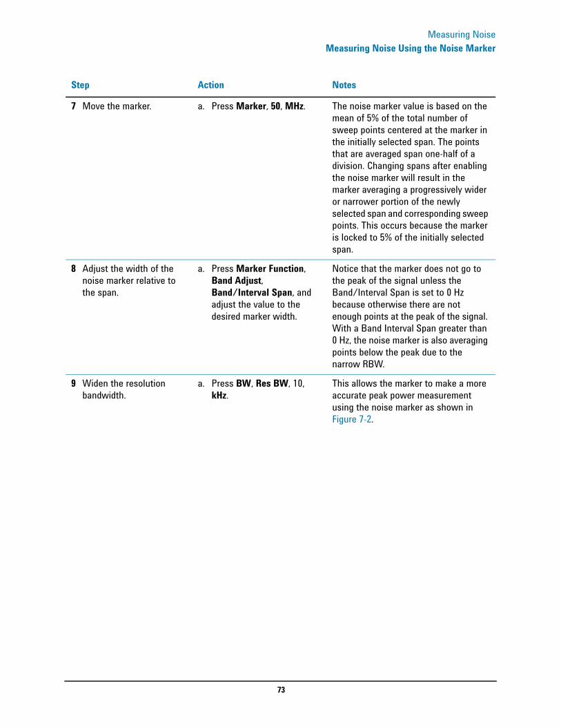
7 Move the marker. a. Press Marker, 50, MHz. The noise marker value is based on the mean of 5% of the total number of sweep points centered at the marker in the initially selected span. The points that are averaged span one-half of a division. Changing spans after enabling the noise marker will result in the marker averaging a progressively wider or narrower portion of the newly selected span and corresponding sweep points. This occurs because the marker is locked to 5% of the initially selected span.
8 Adjust the width of the noise marker relative to the span.
a. Press Marker Function, Band Adjust, Band/Interval Span, and adjust the value to the desired marker width.
Notice that the marker does not go to the peak of the signal unless the Band/Interval Span is set to 0 Hz because otherwise there are not enough points at the peak of the signal. With a Band Interval Span greater than 0 Hz, the noise marker is also averaging points below the peak due to the narrow RBW.
9 Widen the resolution bandwidth.
a. Press BW, Res BW, 10, kHz.
This allows the marker to make a more accurate peak power measurement using the noise marker as shown in Figure 7-2.
Step Action Notes
74
Measuring NoiseMeasuring Noise Using the Noise Marker
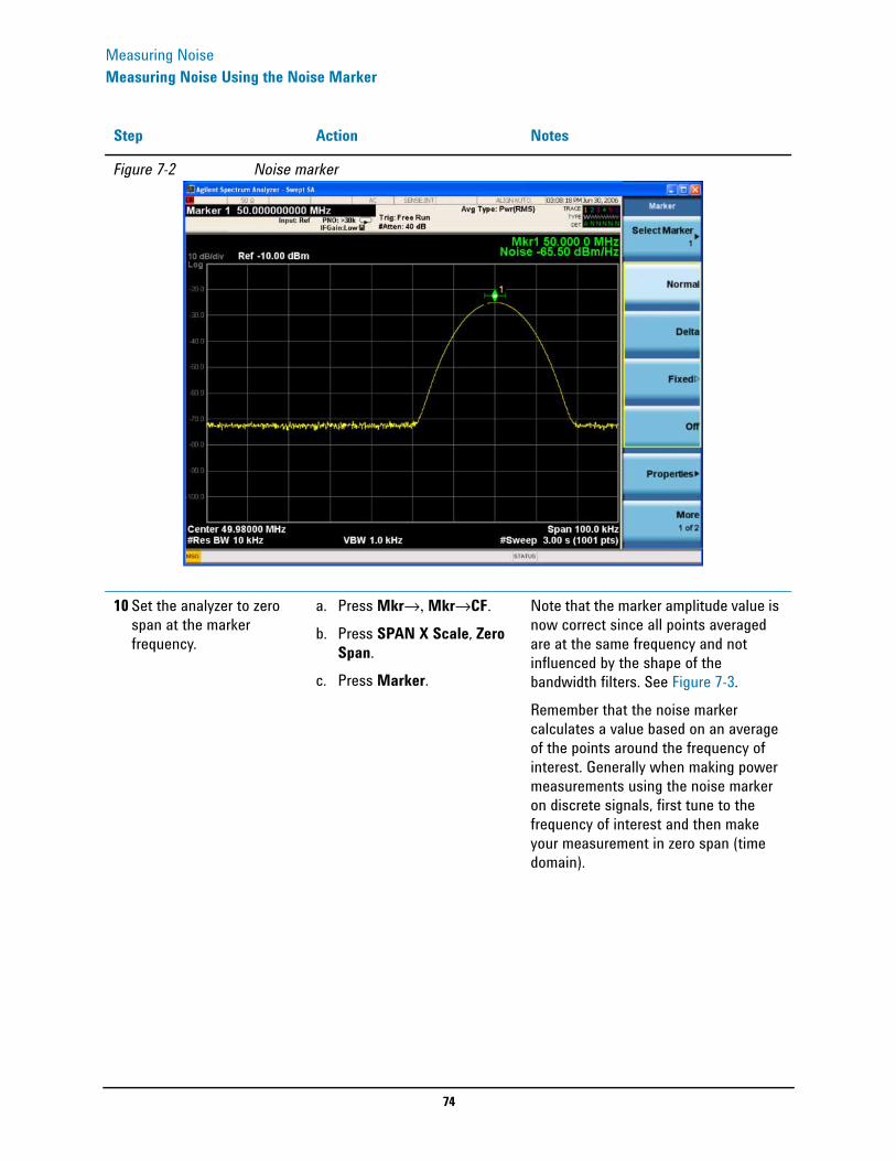
Figure 7-2 Noise marker
10 Set the analyzer to zero span at the marker frequency.
a. Press Mkr→, Mkr→CF.
b. Press SPAN X Scale, Zero Span.
c. Press Marker.
Note that the marker amplitude value is now correct since all points averaged are at the same frequency and not influenced by the shape of the bandwidth filters. See Figure 7-3.Remember that the noise marker calculates a value based on an average of the points around the frequency of interest. Generally when making power measurements using the noise marker on discrete signals, first tune to the frequency of interest and then make your measurement in zero span (time domain).
Step Action Notes

75
Measuring NoiseMeasuring Noise Using the Noise Marker
Figure 7-3 Noise Marker with Zero Span
Step Action Notes
76
Measuring NoiseMeasuring Noise-Like Signals Using Band/Interval Density Markers
Measuring Noise-Like Signals Using Band/Interval Density MarkersBand/Interval Density Markers let you measure power over a frequency span. The markers allow you to easily and conveniently select any arbitrary portion of the displayed signal. However, while the analyzer, when autocoupled, makes sure the analysis is power-responding (rms voltage-responding), you must set all of the other parameters.
Step Action Notes
1 Set the analyzer to the Spectrum Analyzer mode.
a. Press Mode, Spectrum Analyzer. This enables the spectrum analyzer measurements.
2 Preset the analyzer a. Press Mode Preset.
3 Set the center frequency, span, reference level and attenuation.
a. Press FREQ Channel, Center Freq, 50, MHz.
b. Press SPAN X Scale, Span, 100, kHz.
c. Press AMPTD Y Scale, Ref Level, −20, dBm.
d. Press AMPTD Y Scale, Attenuation, 40, dB.
4 Measure the total noise power between the markers.
a. Press Marker Function, Band/Interval Density.
5 Set the band span. a. Press Band Adjust, Band/Interval Span, 40, kHz.
6 Set the resolution and video bandwidths.
a. Press BW, Res BW, 1, kHz.b. Press BW, Video BW, 10, kHz.
Common practice is to set the resolution bandwidth from 1% to 3% of the measurement (marker) span, 40 kHz in this example.
7 Enable the internal 50 MHz amplitude reference signal of the analyzer.
a. Press Input/Output, RF Calibrator, 50 MHz.
Adds a discrete tone to see the effects on the reading. See Figure 7-4.
77
Measuring NoiseMeasuring Noise-Like Signals Using Band/Interval Density Markers
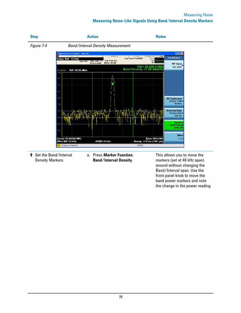
Figure 7-4 Band/Interval Density Measurement
8 Set the Band/Interval Density Markers.
a. Press Marker Function, Band/Interval Density.
This allows you to move the markers (set at 40 kHz span) around without changing the Band/Interval span. Use the front-panel knob to move the band power markers and note the change in the power reading
Step Action Notes
78
Measuring NoiseMeasuring Noise-Like Signals Using Band/Interval Density Markers
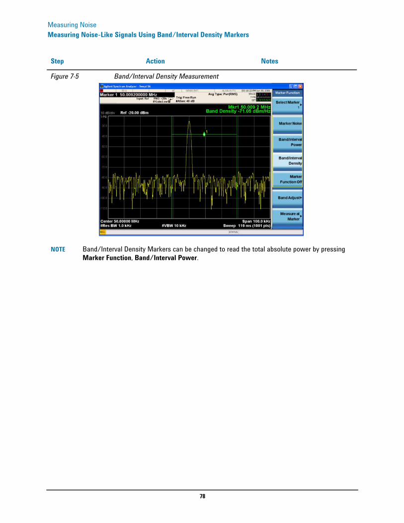
Figure 7-5 Band/Interval Density Measurement
NOTE Band/Interval Density Markers can be changed to read the total absolute power by pressing Marker Function, Band/Interval Power.
Step Action Notes
79
Measuring NoiseMeasuring Noise-Like Signals Using the Channel Power Measurement
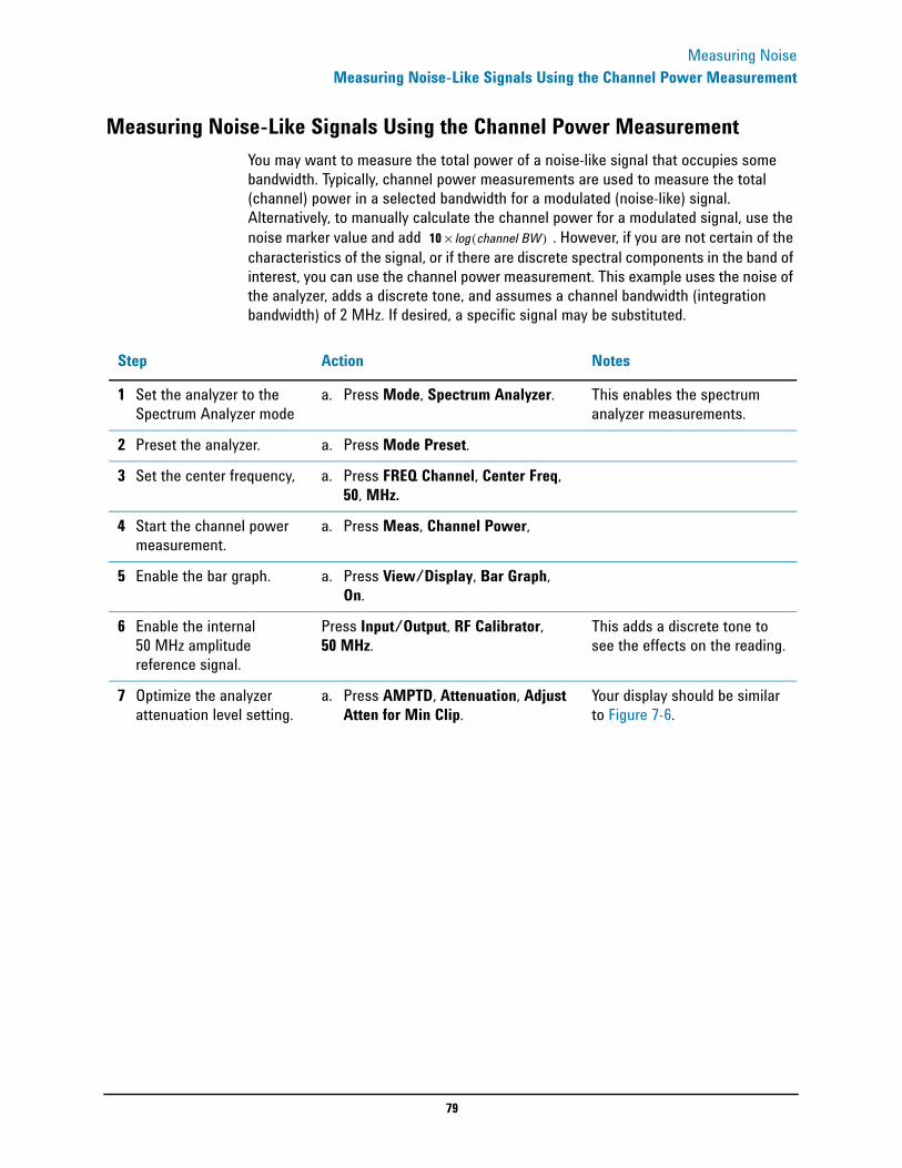
Measuring Noise-Like Signals Using the Channel Power MeasurementYou may want to measure the total power of a noise-like signal that occupies some bandwidth. Typically, channel power measurements are used to measure the total (channel) power in a selected bandwidth for a modulated (noise-like) signal. Alternatively, to manually calculate the channel power for a modulated signal, use the noise marker value and add . However, if you are not certain of the characteristics of the signal, or if there are discrete spectral components in the band of interest, you can use the channel power measurement. This example uses the noise of the analyzer, adds a discrete tone, and assumes a channel bandwidth (integration bandwidth) of 2 MHz. If desired, a specific signal may be substituted.
10 log channel BW( )×
Step Action Notes
1 Set the analyzer to the Spectrum Analyzer mode
a. Press Mode, Spectrum Analyzer. This enables the spectrum analyzer measurements.
2 Preset the analyzer. a. Press Mode Preset.
3 Set the center frequency, a. Press FREQ Channel, Center Freq, 50, MHz.
4 Start the channel power measurement.
a. Press Meas, Channel Power,
5 Enable the bar graph. a. Press View/Display, Bar Graph, On.
6 Enable the internal 50 MHz amplitude reference signal.
Press Input/Output, RF Calibrator, 50 MHz.
This adds a discrete tone to see the effects on the reading.
7 Optimize the analyzer attenuation level setting.
a. Press AMPTD, Attenuation, Adjust Atten for Min Clip.
Your display should be similar to Figure 7-6.
80
Measuring NoiseMeasuring Noise-Like Signals Using the Channel Power Measurement
The power reading is essentially that of the tone; that is, the total noise power is far enough below that of the tone that the noise power contributes very little to the total.
The algorithm that computes the total power works equally well for signals of any statistical variant, whether tone-like, noise-like, or combination.
Figure 7-6 Measuring Channel Power
Step Action Notes
81
Measuring NoiseMeasuring Signal-to-Noise of a Modulated Carrier
Measuring Signal-to-Noise of a Modulated CarrierSignal-to-noise (or carrier-to-noise) is a ratio used in many communication systems as indication of the noise performance in the system. Typically, the more signals added to the system or an increase in the complexity of the modulation scheme can add to the noise level. This can reduce the signal-to-noise ratio and impact the quality of the demodulated signal. For example, a reduced signal-to-noise in digital systems may cause an increase in EVM (error vector magnitude).
With modern complex digital modulation schemes, measuring the modulated carrier requires capturing all of its power accurately. This procedure uses the Band Power Marker with a RMS average detector to correctly measure the carrier's power within a user adjustable region. A Noise Marker (normalized to a 1 Hz noise power bandwidth) with an adjustable noise region is also employed to allow the user to select and accurately measure just the system noise of interest. An important key to making accurate Band Power Marker and Noise Power measurements is to insure that the Average Type under the Meas Setup key is set to “Auto”.
In this example a 4 carrier W-CDMA digitally modulated carrier is used as the fundamental signal and the internal noise of the analyzer is measured as the system noise.
Step Action Notes
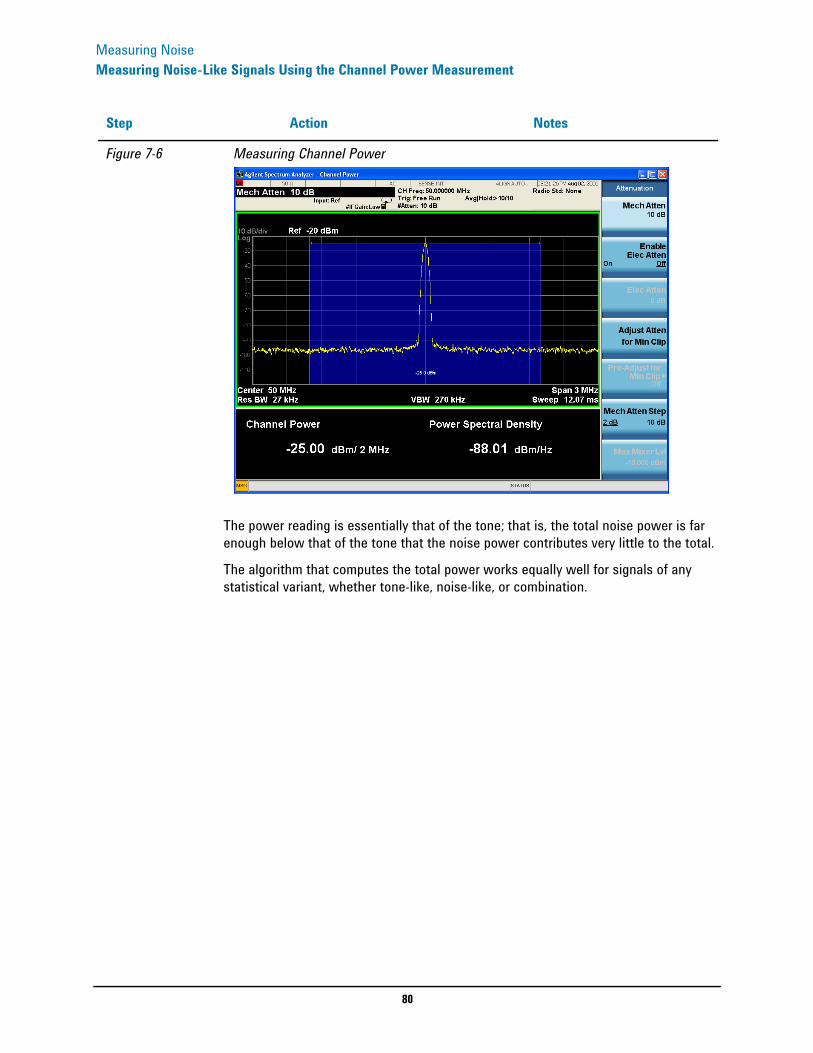
1 Setup the signal sources. a. Setup a 4 carrier W-CDMA signal.b. Set the source frequency to 1.96 GHz.c. Set the source amplitude to –10 dBm.
2 Instrument setup. a. Connect the source RF OUTPUT to the analyzer RF INPUT as shown.
3 Set the analyzer to the Spectrum Analyzer mode.
a. Press Mode, Spectrum Analyzer This enables the spectrum analyzer measurements
4 Preset the analyzer. a. Press Mode Preset.
5 Tune to the W-CDMA signal.
a. Press FREQ Channel, Auto Tune.
82
Measuring NoiseMeasuring Signal-to-Noise of a Modulated Carrier
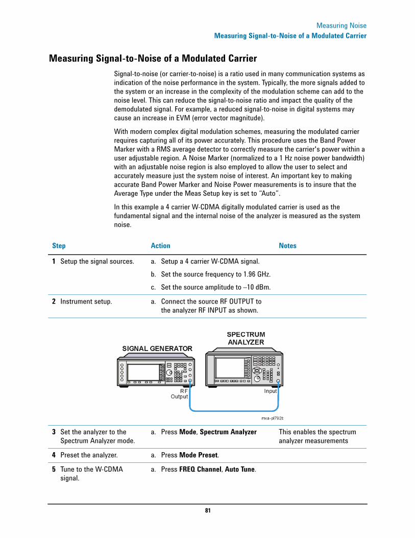
6 Enable the Band Power Marker function.
a. Press Marker Function, Band/Interval Power.
This measures the total power of the 4 carrier W-CDMA signal.
7 Center the frequency of the Band Power marker on the signal.
a. Press Select Marker 1, 1.96, GHz
8 Adjust the width (or span) of the Band Power marker.
a. Press Marker Function, Band Adjust, Band/Interval Span, 20, MHz.
This encompasses the entire 4 carrier W-CDMA signal.
Figure 7-7 4 Carrier W-CDMA Signal Power using Band Power Marker
Note the green vertical lines of Marker 1 representing the span of signals included in the Band Power measurement and the carrier power indicated in Markers Result Block.
9 Enable the Noise Marker using marker 2.
a. Press Marker Function, Select Marker, Marker 2, Marker Noise.
This measures the system noise power.
10 Move the Noise Marker 2 to the system noise frequency of interest.
a. Press Select Marker 2, 1.979, GHz. This encompasses the desired noise power.
11 Adjust the width of the noise marker region.
a. Press Marker Function, Select Marker, Marker 2, Band Adjust, Band/Interval, 5, MHz.
See Figure 7-8.
Step Action Notes
83
Measuring NoiseMeasuring Signal-to-Noise of a Modulated Carrier
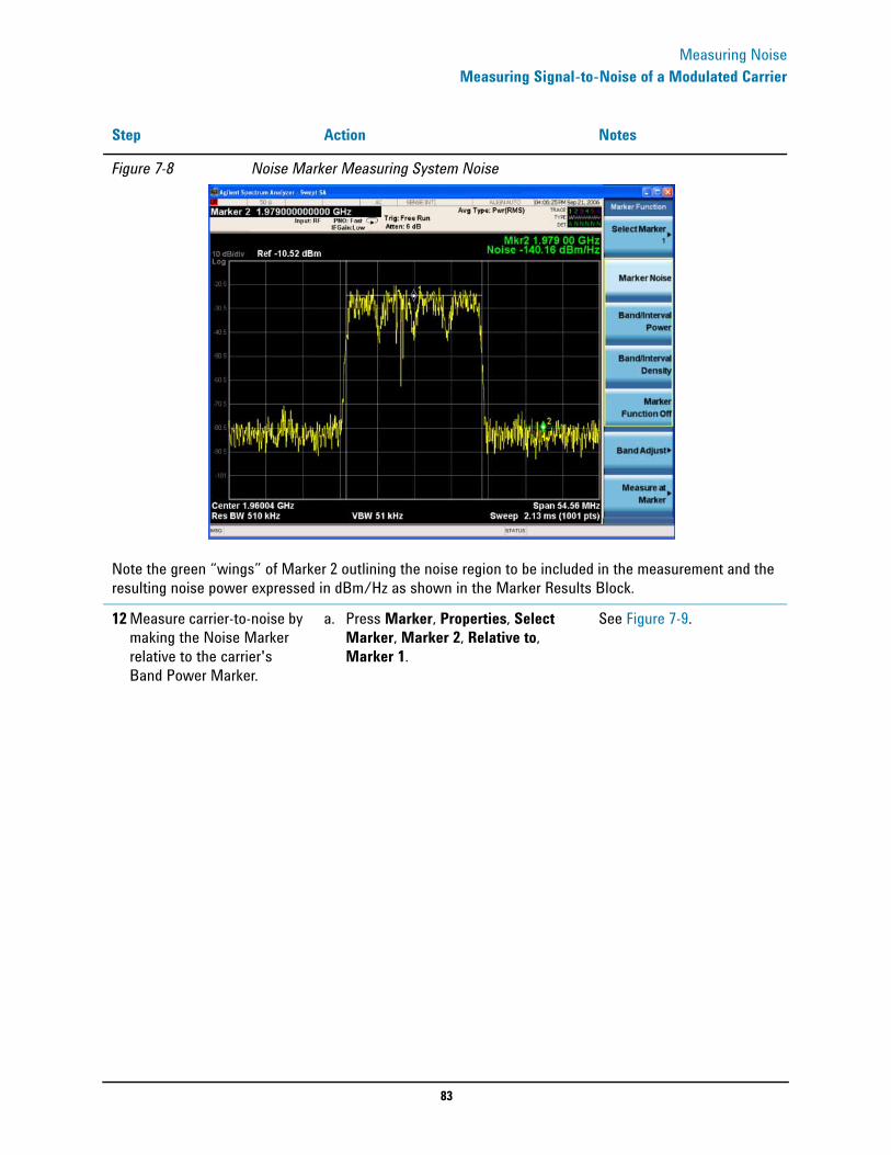
Figure 7-8 Noise Marker Measuring System Noise
Note the green “wings” of Marker 2 outlining the noise region to be included in the measurement and the resulting noise power expressed in dBm/Hz as shown in the Marker Results Block.
12 Measure carrier-to-noise by making the Noise Marker relative to the carrier's Band Power Marker.
a. Press Marker, Properties, Select Marker, Marker 2, Relative to, Marker 1.
See Figure 7-9.
Step Action Notes
84
Measuring NoiseMeasuring Signal-to-Noise of a Modulated Carrier
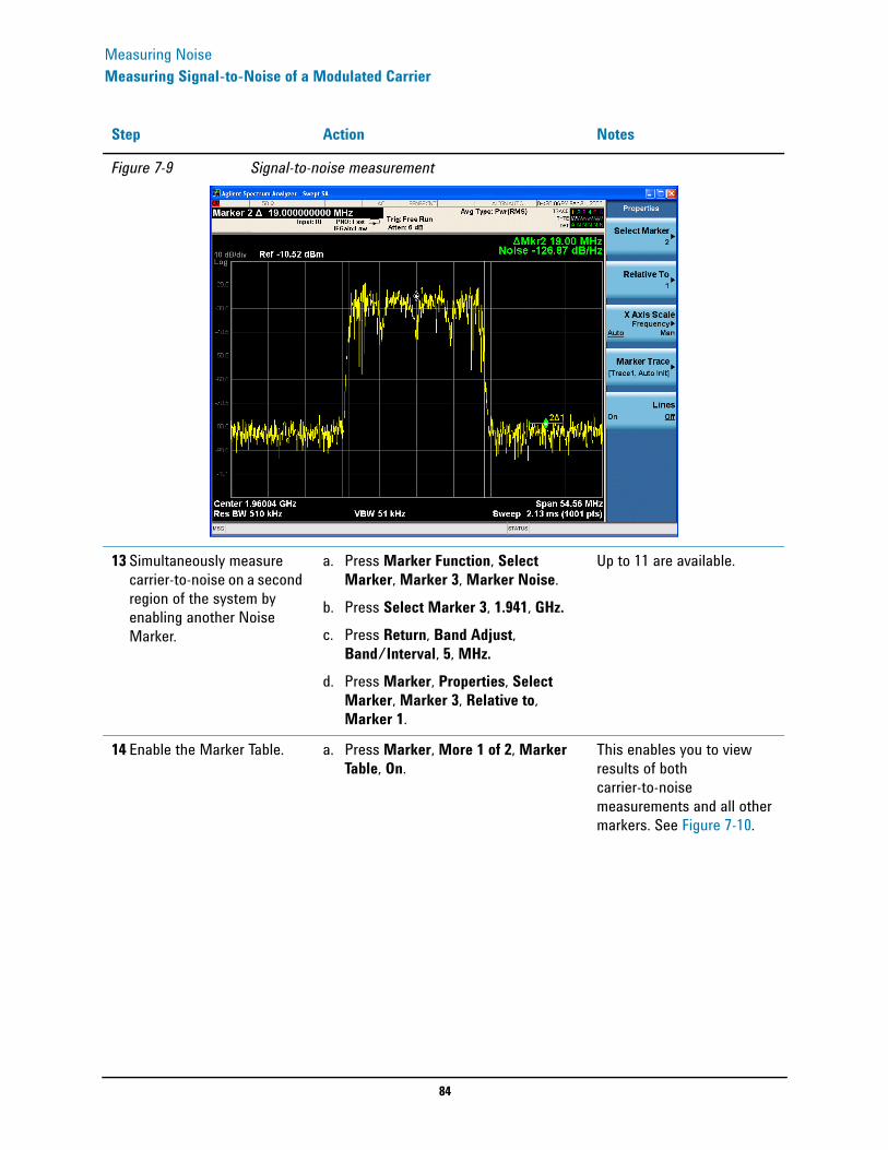
Figure 7-9 Signal-to-noise measurement
13 Simultaneously measure carrier-to-noise on a second region of the system by enabling another Noise Marker.
a. Press Marker Function, Select Marker, Marker 3, Marker Noise.
b. Press Select Marker 3, 1.941, GHz.c. Press Return, Band Adjust,
Band/Interval, 5, MHz.d. Press Marker, Properties, Select
Marker, Marker 3, Relative to, Marker 1.
Up to 11 are available.
14 Enable the Marker Table. a. Press Marker, More 1 of 2, Marker Table, On.
This enables you to view results of both carrier-to-noise measurements and all other markers. See Figure 7-10.
Step Action Notes
85
Measuring NoiseMeasuring Signal-to-Noise of a Modulated Carrier
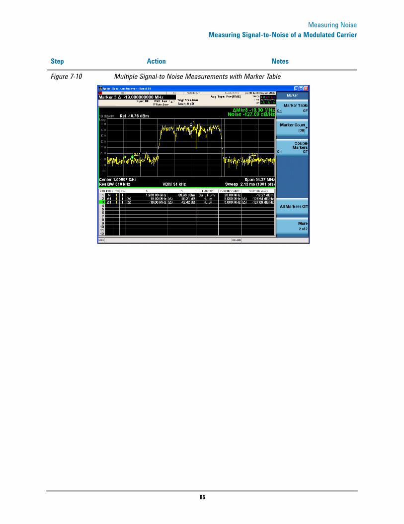
Figure 7-10 Multiple Signal-to Noise Measurements with Marker Table
Step Action Notes

86
Measuring NoiseImproving Phase Noise Measurements by Subtracting Signal Analyzer Noise
Improving Phase Noise Measurements by Subtracting Signal Analyzer NoiseMaking noise power measurements (such as phase noise) near the noise floor of the signal analyzer can be challenging where every dB improvement is important. Utilizing the analyzer trace math function Power Diff and 3 separate traces allows measurement of the DUT phase noise in one trace, the analyzer noise floor in a second trace and then the resulting subtraction of those two traces displayed in a third trace with the analyzer noise contribution removed.
Step Action Notes
1 Setup the signal sources. a. Setup an unmodulated signal.b. Set the source frequency to 1.96 GHz.c. Set the source amplitude to –30 dBm.
2 Instrument setup. a. Connect the source RF OUTPUT to the analyzer RF INPUT as shown.
3 Set the analyzer to the Spectrum Analyzer mode.
a. Press Mode, Spectrum Analyzer. This enables the spectrum analyzer measurements.
4 Preset the analyzer. a. Press Mode Preset.
5 Tune to the unmodulated carrier, adjust the span and RBW.
a. Press FREQ Channel, Auto Tune.b. Press Span, Span, 200, kHz.c. Press BW, Res BW, 910, Hz.
6 Measure and store the DUT phase noise plus the analyzer noise.
a. Press Trace/Detector, Select Trace, Trace 1, Trace AverageAfter sufficient averaging:
b. Press View/Blank, View
Allow time for sufficient averaging before initiating action b.See Figure 7-11.
87
Measuring NoiseImproving Phase Noise Measurements by Subtracting Signal Analyzer Noise
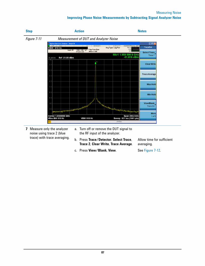
Figure 7-11 Measurement of DUT and Analyzer Noise
7 Measure only the analyzer noise using trace 2 (blue trace) with trace averaging.
a. Turn off or remove the DUT signal to the RF input of the analyzer.
b. Press Trace/Detector, Select Trace, Trace 2, Clear Write, Trace Average.
c. Press View/Blank, View.
Allow time for sufficient averaging.See Figure 7-12.
Step Action Notes

88
Measuring NoiseImproving Phase Noise Measurements by Subtracting Signal Analyzer Noise
Figure 7-12 Measurement of Analyzer Noise
8 Subtract the noise from the DUT phase noise measurement using the Power Diff math function.
a. Press Trace/Detector, Select Trace, Trace 3, Clear Write.
b. Press More, More, Math, Power Diff, Trace Operands, Operand 1, Trace 1, Operand 2, Trace 2.
Notice the phase noise improvement at 100 kHz offset between trace 1 (yellow trace) and trace 3 (magenta trace).See Figure 7-13.
Step Action Notes
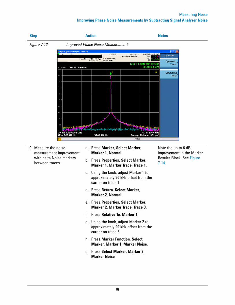
89
Measuring NoiseImproving Phase Noise Measurements by Subtracting Signal Analyzer Noise
Figure 7-13 Improved Phase Noise Measurement
9 Measure the noise measurement improvement with delta Noise markers between traces.
a. Press Marker, Select Marker, Marker 1, Normal.
b. Press Properties, Select Marker, Marker 1, Marker Trace, Trace 1.
c. Using the knob, adjust Marker 1 to approximately 90 kHz offset from the carrier on trace 1.
d. Press Return, Select Marker, Marker 2, Normal.
e. Press Properties, Select Marker, Marker 2, Marker Trace, Trace 3.
f. Press Relative To, Marker 1.g. Using the knob, adjust Marker 2 to
approximately 90 kHz offset from the carrier on trace 3.
h. Press Marker Function, Select Marker, Marker 1, Marker Noise.
i. Press Select Marker, Marker 2, Marker Noise.
Note the up to 6 dB improvement in the Marker Results Block. See Figure 7-14.
Step Action Notes

90
Measuring NoiseImproving Phase Noise Measurements by Subtracting Signal Analyzer Noise
Figure 7-14 Improved Phase Noise Measurement with Delta Noise Markers
Step Action Notes
91
Making Time-Gated Measurements
8 Making Time-Gated Measurements
Traditional frequency-domain spectrum analysis provides only limited information for certain signals. Examples of these difficult-to-analyze signal include the following:
• Pulsed-RF• Time multiplexed• Interleaved or intermittent• Time domain multiple access (TDMA) radio formats• Modulated burstThe time gating measurement examples use a simple frequency-modulated, pulsed-RF signal. The goal is to eliminate the pulse spectrum and then view the spectrum of the FM carrier as if it were continually on, rather than pulsed. This reveals low-level modulation components that are hidden by the pulse spectrum.
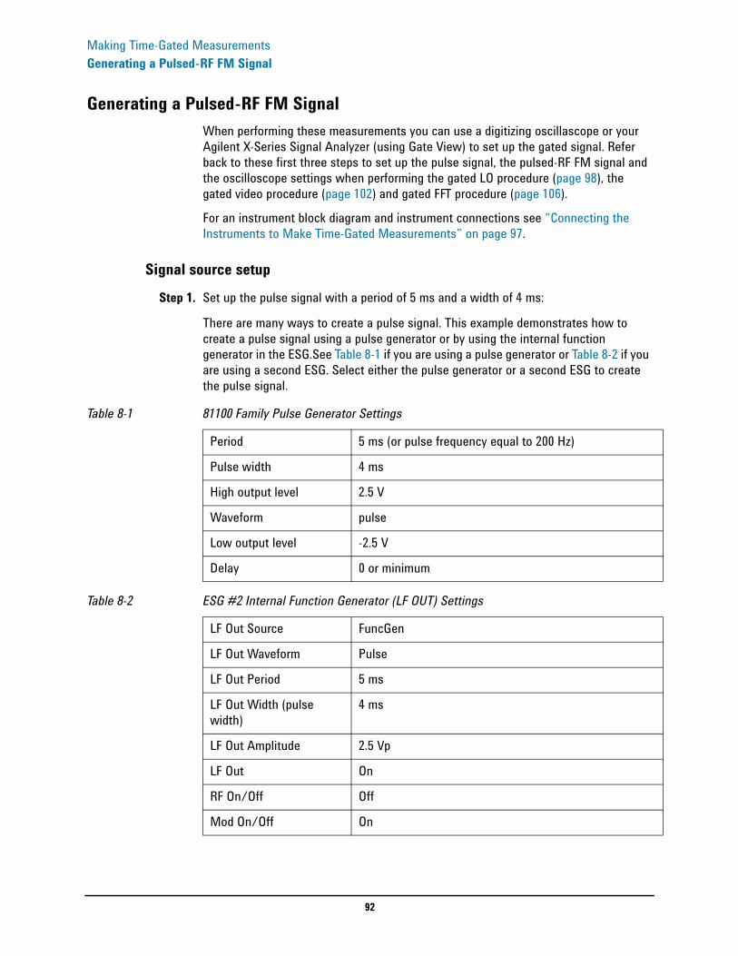
92
Making Time-Gated MeasurementsGenerating a Pulsed-RF FM Signal
Generating a Pulsed-RF FM SignalWhen performing these measurements you can use a digitizing oscillascope or your Agilent X-Series Signal Analyzer (using Gate View) to set up the gated signal. Refer back to these first three steps to set up the pulse signal, the pulsed-RF FM signal and the oscilloscope settings when performing the gated LO procedure (page 98), the gated video procedure (page 102) and gated FFT procedure (page 106).
For an instrument block diagram and instrument connections see “Connecting the Instruments to Make Time-Gated Measurements” on page 97.
Signal source setupStep 1. Set up the pulse signal with a period of 5 ms and a width of 4 ms:
There are many ways to create a pulse signal. This example demonstrates how to create a pulse signal using a pulse generator or by using the internal function generator in the ESG.See Table 8-1 if you are using a pulse generator or Table 8-2 if you are using a second ESG. Select either the pulse generator or a second ESG to create the pulse signal.
Table 8-1 81100 Family Pulse Generator Settings
Period 5 ms (or pulse frequency equal to 200 Hz)
Pulse width 4 ms
High output level 2.5 V
Waveform pulse
Low output level -2.5 V
Delay 0 or minimum
Table 8-2 ESG #2 Internal Function Generator (LF OUT) Settings
LF Out Source FuncGen
LF Out Waveform Pulse
LF Out Period 5 ms
LF Out Width (pulse width)
4 ms
LF Out Amplitude 2.5 Vp
LF Out On
RF On/Off Off
Mod On/Off On
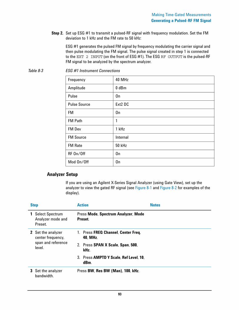
93
Making Time-Gated MeasurementsGenerating a Pulsed-RF FM Signal
Step 2. Set up ESG #1 to transmit a pulsed-RF signal with frequency modulation. Set the FM deviation to 1 kHz and the FM rate to 50 kHz:
ESG #1 generates the pulsed FM signal by frequency modulating the carrier signal and then pulse modulating the FM signal. The pulse signal created in step 1 is connected to the EXT 2 INPUT (on the front of ESG #1). The ESG RF OUTPUT is the pulsed-RF FM signal to be analyzed by the spectrum analyzer.
Analyzer SetupIf you are using an Agilent X-Series Signal Analyzer (using Gate View), set up the analyzer to view the gated RF signal (see Figure 8-1 and Figure 8-2 for examples of the display).
Table 8-3 ESG #1 Instrument Connections
Frequency 40 MHz
Amplitude 0 dBm
Pulse On
Pulse Source Ext2 DC
FM On
FM Path 1
FM Dev 1 kHz
FM Source Internal
FM Rate 50 kHz
RF On/Off On
Mod On/Off On
Step Action Notes
1 Select Spectrum Analyzer mode and Preset.
Press Mode, Spectrum Analyzer, Mode Preset.
2 Set the analyzer center frequency, span and reference level.
1. Press FREQ Channel, Center Freq, 40, MHz.
2. Press SPAN X Scale, Span, 500, kHz.
3. Press AMPTD Y Scale, Ref Level, 10, dBm.
3 Set the analyzer bandwidth.
Press BW, Res BW (Man), 100, kHz.
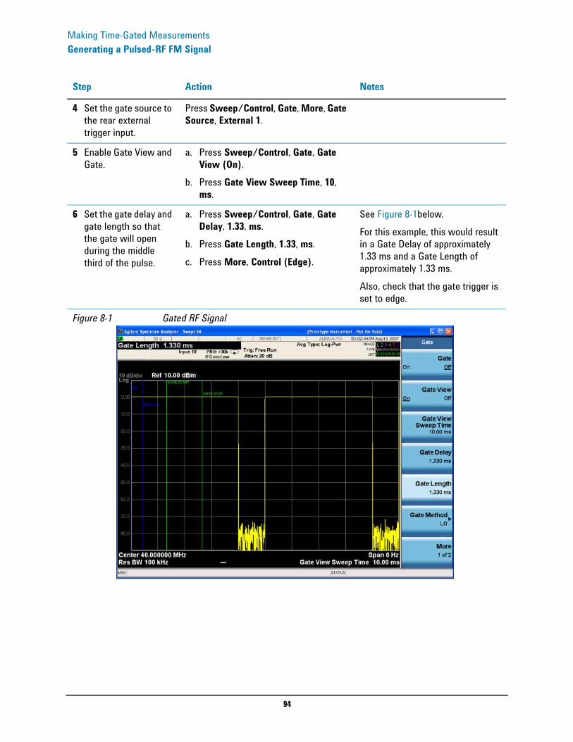
94
Making Time-Gated MeasurementsGenerating a Pulsed-RF FM Signal
4 Set the gate source to the rear external trigger input.
Press Sweep/Control, Gate, More, Gate Source, External 1.
5 Enable Gate View and Gate.
a. Press Sweep/Control, Gate, Gate View (On).
b. Press Gate View Sweep Time, 10, ms.
6 Set the gate delay and gate length so that the gate will open during the middle third of the pulse.
a. Press Sweep/Control, Gate, Gate Delay, 1.33, ms.
b. Press Gate Length, 1.33, ms.c. Press More, Control (Edge).
See Figure 8-1below.For this example, this would result in a Gate Delay of approximately 1.33 ms and a Gate Length of approximately 1.33 ms. Also, check that the gate trigger is set to edge.
Figure 8-1 Gated RF Signal
Step Action Notes
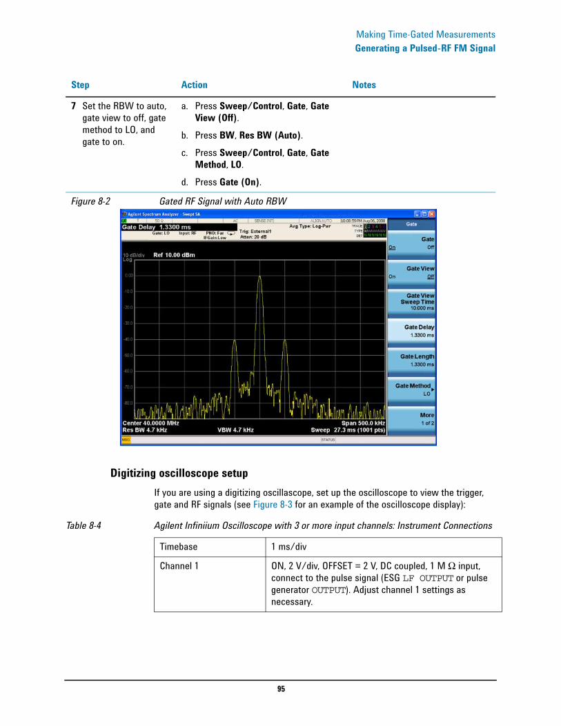
95
Making Time-Gated MeasurementsGenerating a Pulsed-RF FM Signal
Digitizing oscilloscope setupIf you are using a digitizing oscillascope, set up the oscilloscope to view the trigger, gate and RF signals (see Figure 8-3 for an example of the oscilloscope display):
7 Set the RBW to auto, gate view to off, gate method to LO, and gate to on.
a. Press Sweep/Control, Gate, Gate View (Off).
b. Press BW, Res BW (Auto).c. Press Sweep/Control, Gate, Gate
Method, LO.d. Press Gate (On).
Figure 8-2 Gated RF Signal with Auto RBW
Step Action Notes
Table 8-4 Agilent Infiniium Oscilloscope with 3 or more input channels: Instrument Connections
Timebase 1 ms/div
Channel 1 ON, 2 V/div, OFFSET = 2 V, DC coupled, 1 M Ω input, connect to the pulse signal (ESG LF OUTPUT or pulse generator OUTPUT). Adjust channel 1 settings as necessary.
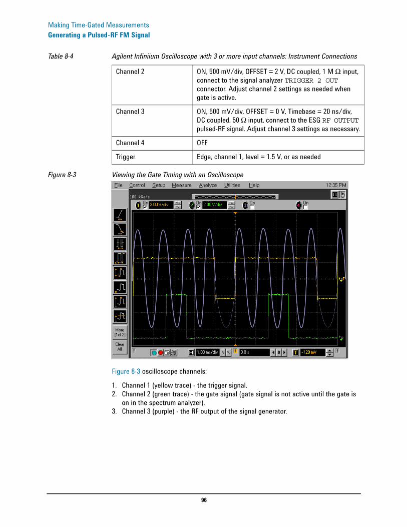
96
Making Time-Gated MeasurementsGenerating a Pulsed-RF FM Signal
Figure 8-3 Viewing the Gate Timing with an Oscilloscope
Figure 8-3 oscilloscope channels:
1. Channel 1 (yellow trace) - the trigger signal.2. Channel 2 (green trace) - the gate signal (gate signal is not active until the gate is
on in the spectrum analyzer).3. Channel 3 (purple) - the RF output of the signal generator.
Channel 2 ON, 500 mV/div, OFFSET = 2 V, DC coupled, 1 M Ω input, connect to the signal analyzer TRIGGER 2 OUT connector. Adjust channel 2 settings as needed when gate is active.
Channel 3 ON, 500 mV/div, OFFSET = 0 V, Timebase = 20 ns/div, DC coupled, 50 Ω input, connect to the ESG RF OUTPUT pulsed-RF signal. Adjust channel 3 settings as necessary.
Channel 4 OFF
Trigger Edge, channel 1, level = 1.5 V, or as needed
Table 8-4 Agilent Infiniium Oscilloscope with 3 or more input channels: Instrument Connections

97
Making Time-Gated MeasurementsConnecting the Instruments to Make Time-Gated Measurements
Connecting the Instruments to Make Time-Gated MeasurementsFigure 8-4 shows a diagram of the test setup. ESG #1 produces a pulsed FM signal by using an external pulse signal. The external pulse signal is connected to the front of the ESG #1 to the EXT 2 INPUT to control the pulsing. The pulse signal is also used as the trigger signal. The oscilloscope is useful for illustrating timing interactions between the trigger signal and the gate. The Gate View feature of the X-Series signal analyzer could be used in place of the oscilloscope.
Using this measurement setup allows you to view all signal spectra on the spectrum analyzer and all timing signals on the oscilloscope. This setup is helpful when you perform gated measurements on unknown signals. If an oscilloscope is not available, begin by using the Gate View feature to set up the gate parameters and then turn Gate View Off to view the signal spectra, refer to Figure 8-5
Figure 8-4 Instrument Connection Diagram with Oscilloscope
Figure 8-5 Instrument Connection Diagram without Oscilloscope
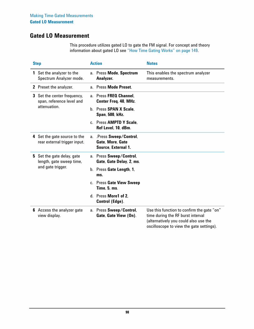
98
Making Time-Gated MeasurementsGated LO Measurement
Gated LO MeasurementThis procedure utilizes gated LO to gate the FM signal. For concept and theory information about gated LO see “How Time Gating Works” on page 149.
Step Action Notes
1 Set the analyzer to the Spectrum Analyzer mode.
a. Press Mode, Spectrum Analyzer.
This enables the spectrum analyzer measurements.
2 Preset the analyzer. a. Press Mode Preset.
3 Set the center frequency, span, reference level and attenuation.
a. Press FREQ Channel, Center Freq, 40, MHz.
b. Press SPAN X Scale, Span, 500, kHz.
c. Press AMPTD Y Scale, Ref Level, 10, dBm.
4 Set the gate source to the rear external trigger input.
a. .Press Sweep/Control, Gate, More, Gate Source, External 1.
5 Set the gate delay, gate length, gate sweep time, and gate trigger.
a. Press Sweep/Control, Gate, Gate Delay, 2, ms.
b. Press Gate Length, 1, ms.
c. Press Gate View Sweep Time, 5, ms.
d. Press More1 of 2, Control (Edge).
6 Access the analyzer gate view display.
a. Press Sweep/Control, Gate, Gate View (On).
Use this function to confirm the gate “on” time during the RF burst interval (alternatively you could also use the oscilloscope to view the gate settings).
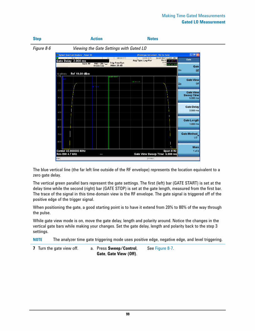
99
Making Time-Gated MeasurementsGated LO Measurement
Figure 8-6 Viewing the Gate Settings with Gated LO
The blue vertical line (the far left line outside of the RF envelope) represents the location equivalent to a zero gate delay.The vertical green parallel bars represent the gate settings. The first (left) bar (GATE START) is set at the delay time while the second (right) bar (GATE STOP) is set at the gate length, measured from the first bar. The trace of the signal in this time-domain view is the RF envelope. The gate signal is triggered off of the positive edge of the trigger signal.When positioning the gate, a good starting point is to have it extend from 20% to 80% of the way through the pulse.While gate view mode is on, move the gate delay, length and polarity around. Notice the changes in the vertical gate bars while making your changes. Set the gate delay, length and polarity back to the step 3 settings.NOTE The analyzer time gate triggering mode uses positive edge, negative edge, and level triggering.
7 Turn the gate view off. a. Press Sweep/Control, Gate, Gate View (Off).
See Figure 8-7.
Step Action Notes
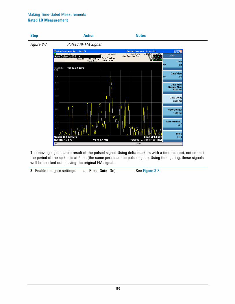
100
Making Time-Gated MeasurementsGated LO Measurement
Figure 8-7 Pulsed RF FM Signal
The moving signals are a result of the pulsed signal. Using delta markers with a time readout, notice that the period of the spikes is at 5 ms (the same period as the pulse signal). Using time gating, these signals well be blocked out, leaving the original FM signal.
8 Enable the gate settings. a. Press Gate (On). See Figure 8-8.
Step Action Notes
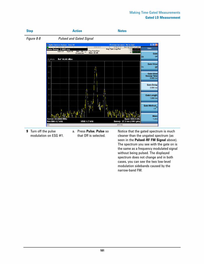
101
Making Time-Gated MeasurementsGated LO Measurement
Figure 8-8 Pulsed and Gated Signal
9 Turn off the pulse modulation on ESG #1.
a. Press Pulse, Pulse so that Off is selected.
Notice that the gated spectrum is much cleaner than the ungated spectrum (as seen in the Pulsed-RF FM Signal above). The spectrum you see with the gate on is the same as a frequency modulated signal without being pulsed. The displayed spectrum does not change and in both cases, you can see the two low-level modulation sidebands caused by the narrow-band FM.
Step Action Notes

102
Making Time-Gated MeasurementsGated Video Measurement
Gated Video Measurement This procedure utilizes gated video to gate the FM signal. For concept and theory information about gated video see “How Time Gating Works” on page 148.
Step Action Notes
1 Set the analyzer to the Spectrum Analyzer mode.
a. Press Mode, Spectrum Analyzer.
This enables the spectrum analyzer measurements.
2 Preset the analyzer a. Press Mode Preset.
3 Set the center frequency, span, reference level and attenuation.
a. Press FREQ Channel, Center Freq, 40, MHz.
b. Press SPAN X Scale, Span, 500, kHz.
c. Press AMPTD Y Scale, Ref Level, 10, dBm.
4 Set analyzer points to 401 and sweep time to 2000 ms.
a. Press Sweep/Control, Points, 401, Enter.
b. Press Sweep Time, 2000, ms.
For gated video, the calculated sweep time should be set to at least
to ensure that the gate is on at least once during each of the 401 sweep points. In this example, the PRI is 5 ms, so you should set the sweep time to 401 minus 1 times 5 ms, or 2 s. If the sweep time is set too fast, some trace points may show values of zero power or other incorrect low readings. If the trace seems incomplete or erratic, try a longer sweep time.
Good practices for determining the minimum sweep time for gated video:In the event that the signal is not noisy, the sweep time can be set to less than
(as calculated above). Instead of using PRI in the previous sweep time calculation, we can use the “gate off time” where sweep time equals
. (Gate off time is defined as , where GL = Gate Length.) In our example we could use a sweep time of 400 points times 1 ms or 400 ms –
. Increase the video bandwidth to improve the probability of capturing the pulse using “gate off time”. If trace points are still showing values of zero power, increase the sweep time by small increments until there are no more dropouts.
5 Set the Gate source to the external trigger input on the rear panel:
a. Press Sweep/Control, Gate, More, Gate Source, External 1.
# sweep points 1–( ) PRI (pulse repetition interval× )
# sweep points 1–( ) PRI (pulse repetition interval× )
# sweep points 1–( ) gate off time× PRI GL–
401 1–( ) 5ms 4ms–( )× 400ms=

103
Making Time-Gated MeasurementsGated Video Measurement
Figure 8-9 Viewing a Pulsed RF FM Signal (without gating)
6 Set the gate delay and gate length.
a. Press Sweep/Control, Gate, More, Control (Edge).
b. Press More, Gate Delay, 2, ms.
c. Press Gate Length, 1, ms.
Ensure that the gate control is set to Edge.
7 Turn the gate on. a. Press Sweep/Control, Gate, Gate Method, Video.
b. Press Gate (On).
Step Action Notes
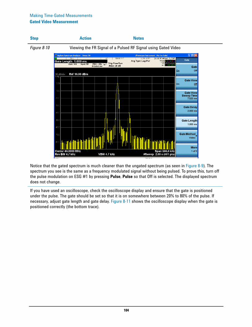
104
Making Time-Gated MeasurementsGated Video Measurement
Figure 8-10 Viewing the FR Signal of a Pulsed RF Signal using Gated Video
Notice that the gated spectrum is much cleaner than the ungated spectrum (as seen in Figure 8-9). The spectrum you see is the same as a frequency modulated signal without being pulsed. To prove this, turn off the pulse modulation on ESG #1 by pressing Pulse, Pulse so that Off is selected. The displayed spectrum does not change.
If you have used an oscilloscope, check the oscilloscope display and ensure that the gate is positioned under the pulse. The gate should be set so that it is on somewhere between 20% to 80% of the pulse. If necessary, adjust gate length and gate delay. Figure 8-11 shows the oscilloscope display when the gate is positioned correctly (the bottom trace).
Step Action Notes
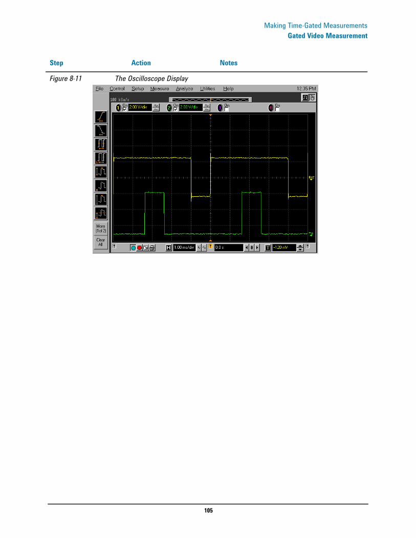
105
Making Time-Gated MeasurementsGated Video Measurement
Figure 8-11 The Oscilloscope Display
Step Action Notes

106
Making Time-Gated MeasurementsGated FFT Measurement
Gated FFT Measurement This procedure utilizes gated FFT to gate the FM signal. For concept and theory information about gated FFT see “How Time Gating Works” on page 149.
Step Action Notes
1 Set the analyzer to the Spectrum Analyzer mode.
a. Press Mode, Spectrum Analyzer.
This enables the spectrum analyzer measurements.
2 Preset the analyzer a. Press Mode Preset.
3 Set the center frequency, span, reference level and attenuation.
a. Press FREQ Channel, Center Freq, 40, MHz.
b. Press SPAN X Scale, Span, 500, kHz.
c. Press AMPTD Y Scale, Ref Level, 10, dBm.
4 Set the Gate source to the external trigger input on the rear panel.
a. Press Sweep/Control, Gate, More, Gate Source, External 1.
5 Set the gate method and turn gate on.
a. Press Sweep/Control, Gate, Gate Method, FFT.
b. Press Gate (On).
6 Select the minimum resolution bandwidth required.
a. Press BW, Res BW (Auto).
See Figure 8-12.
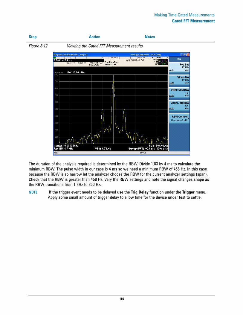
107
Making Time-Gated MeasurementsGated FFT Measurement
Figure 8-12 Viewing the Gated FFT Measurement results
The duration of the analysis required is determined by the RBW. Divide 1.83 by 4 ms to calculate the minimum RBW. The pulse width in our case is 4 ms so we need a minimum RBW of 458 Hz. In this case because the RBW is so narrow let the analyzer choose the RBW for the current analyzer settings (span). Check that the RBW is greater than 458 Hz. Vary the RBW settings and note the signal changes shape as the RBW transitions from 1 kHz to 300 Hz.NOTE If the trigger event needs to be delayed use the Trig Delay function under the Trigger menu.
Apply some small amount of trigger delay to allow time for the device under test to settle.
Step Action Notes

108
Making Time-Gated MeasurementsGated FFT Measurement

109
Measuring Digital Communications Signals
9 Measuring Digital Communications Signals
The Signal Analyzer makes power measurements on digital communication signals fast and repeatable by providing a comprehensive suite of power-based one-button automated measurements with pre-set standards-based format setups. The automated measurements also include pass/fail functionality that allow the user to quickly check if the signal passed the measurement.
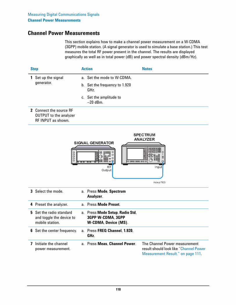
110
Measuring Digital Communications SignalsChannel Power Measurements
Channel Power MeasurementsThis section explains how to make a channel power measurement on a W-CDMA (3GPP) mobile station. (A signal generator is used to simulate a base station.) This test measures the total RF power present in the channel. The results are displayed graphically as well as in total power (dB) and power spectral density (dBm/Hz).
Step Action Notes
1 Set up the signal generator.
a. Set the mode to W-CDMA.b. Set the frequency to 1.920
GHz.c. Set the amplitude to
−20 dBm.
2 Connect the source RF OUTPUT to the analyzer RF INPUT as shown.
3 Select the mode. a. Press Mode, Spectrum Analyzer.
4 Preset the analyzer. a. Press Mode Preset.
5 Set the radio standard and toggle the device to mobile station.
a. Press Mode Setup, Radio Std, 3GPP W-CDMA, 3GPP W-CDMA, Device (MS).
6 Set the center frequency. a. Press FREQ Channel, 1.920, GHz.
7 Initiate the channel power measurement.
a. Press Meas, Channel Power. The Channel Power measurement result should look like “Channel Power Measurement Result.” on page 111.
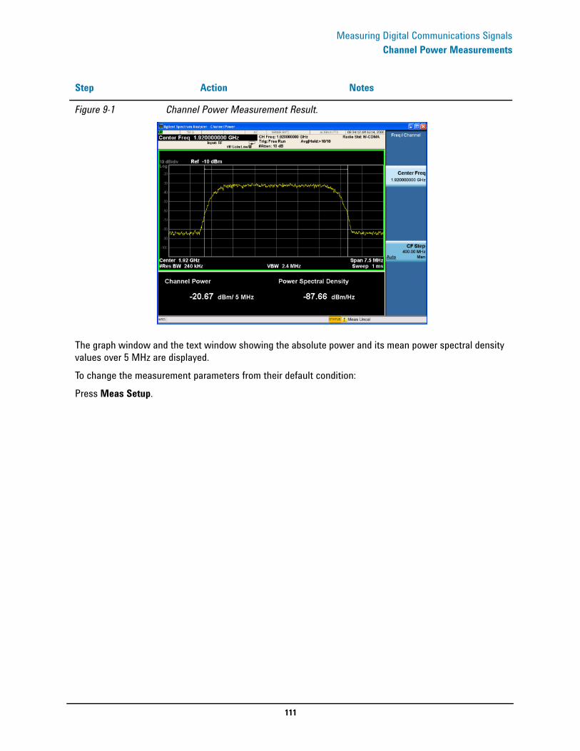
111
Measuring Digital Communications SignalsChannel Power Measurements
Figure 9-1 Channel Power Measurement Result.
The graph window and the text window showing the absolute power and its mean power spectral density values over 5 MHz are displayed.To change the measurement parameters from their default condition:Press Meas Setup.
Step Action Notes

112
Measuring Digital Communications SignalsOccupied Bandwidth Measurements
Occupied Bandwidth MeasurementsThis section explains how to make the occupied bandwidth measurement on a W-CDMA (3GPP) mobile station. (A signal generator is used to simulate a base station.) The instrument measures power across the band, and then calculates its 99.0% power bandwidth.
Step Action Notes
1 Set up the signal generator. a. Set the mode to W-CDMA.b. Set the frequency to 1.920
GHz.c. Set the amplitude to
−20 dBm.
2 Connect the source RF OUTPUT to the analyzer RF INPUT as shown.
3 Select the mode. a. Press Mode, Spectrum Analyzer.
4 Preset the analyzer. a. Press Mode Preset.
5 Set the radio standard and toggle the device to mobile station.
a. Press Mode Setup, Radio Std, 3GPP W-CDMA, 3GPP W-CDMA, Device (MS).
6 Set the center frequency. a. Press FREQ Channel, 1.920, GHz.
7 Initiate the occupied bandwidth measurement.
a. Press Meas, Occupied BW.
The Occupied BW measurement result should look like “Occupied BW Measurement Result” on page 113.
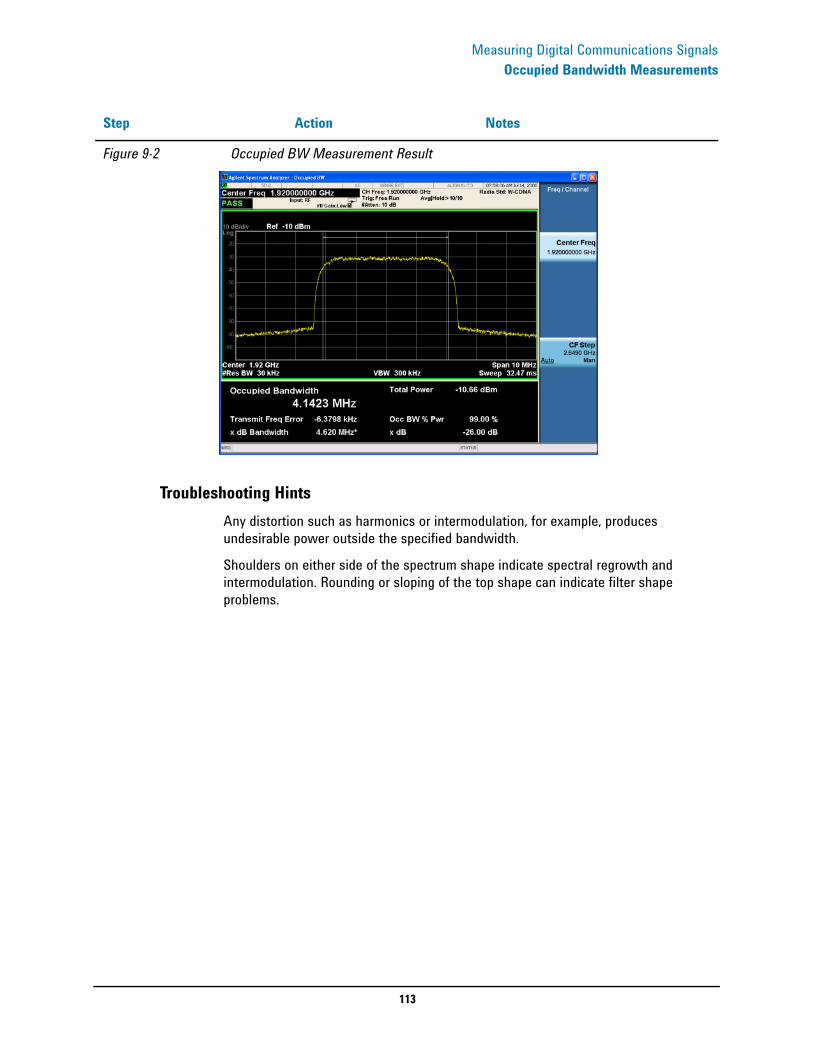
113
Measuring Digital Communications SignalsOccupied Bandwidth Measurements
Troubleshooting HintsAny distortion such as harmonics or intermodulation, for example, produces undesirable power outside the specified bandwidth.
Shoulders on either side of the spectrum shape indicate spectral regrowth and intermodulation. Rounding or sloping of the top shape can indicate filter shape problems.
Figure 9-2 Occupied BW Measurement Result
Step Action Notes

114
Measuring Digital Communications SignalsMaking Adjacent Channel Power (ACP) Measurements
Making Adjacent Channel Power (ACP) MeasurementsThe adjacent channel power (ACP) measurement is also referred to as the adjacent channel power ratio (ACPR) and adjacent channel leakage ratio (ACLR). We use the term ACP to refer to this measurement.
ACP measures the total power (rms voltage) in the specified channel and up to six pairs of offset frequencies. The measurement result reports the ratios of the offset powers to the main channel power.
The following example shows how to make an ACP measurement on a W-CDMA base station signal broadcasting at 1.96 GHz. (A signal generator is used to simulate a base station.)
Step Action Notes
1 Set up the signal generator.
a. Set the mode to W-CDMA.b. Set the frequency to 1.920
GHz.c. Set the amplitude to
−10 dBm.
2 Connect the source RF OUTPUT to the analyzer RF INPUT as shown.
3 Select the mode. a. Press Mode, Spectrum Analyzer.
4 Preset the analyzer. a. Press Mode Preset.
5 Set the analyzer radio mode to W-CDMA as a base station device.
a. Press Mode Setup, Radio Std, 3GPP W-CDMA, 3GPP W-CDMA,
b. Press Mode Setup, Radio Std Setup, Device (BTS).
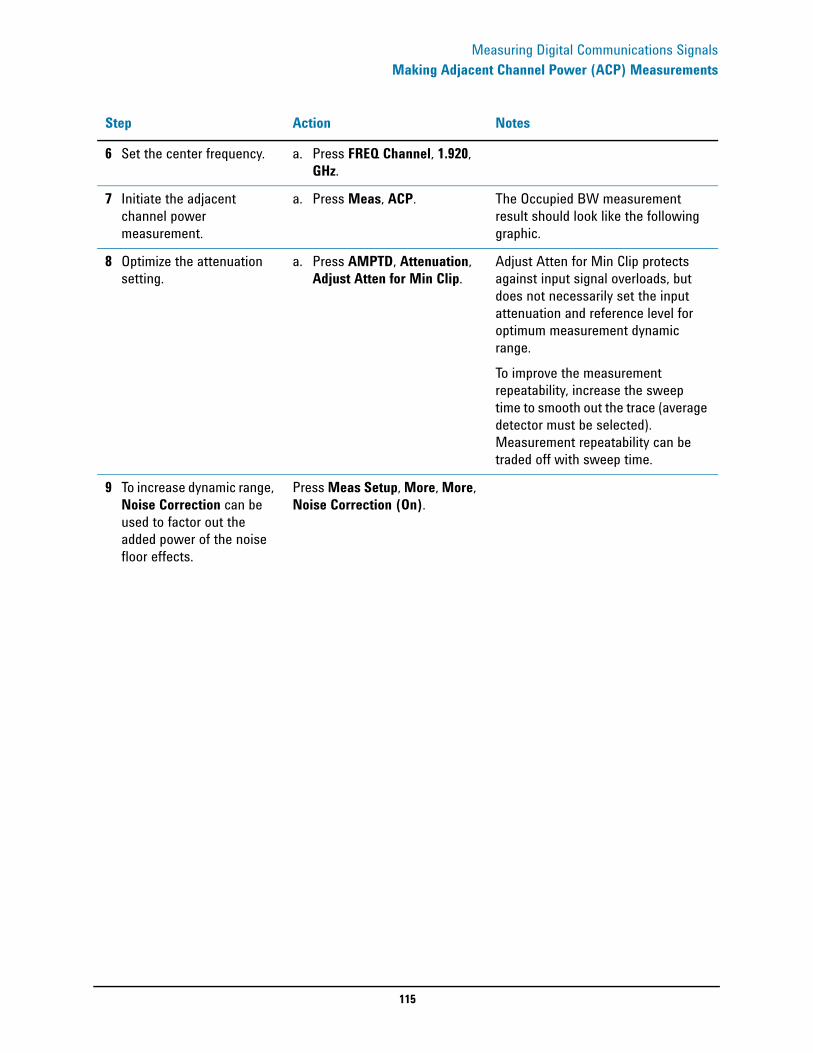
115
Measuring Digital Communications SignalsMaking Adjacent Channel Power (ACP) Measurements
6 Set the center frequency. a. Press FREQ Channel, 1.920, GHz.
7 Initiate the adjacent channel power measurement.
a. Press Meas, ACP. The Occupied BW measurement result should look like the following graphic.
8 Optimize the attenuation setting.
a. Press AMPTD, Attenuation, Adjust Atten for Min Clip.
Adjust Atten for Min Clip protects against input signal overloads, but does not necessarily set the input attenuation and reference level for optimum measurement dynamic range.To improve the measurement repeatability, increase the sweep time to smooth out the trace (average detector must be selected). Measurement repeatability can be traded off with sweep time.
9 To increase dynamic range, Noise Correction can be used to factor out the added power of the noise floor effects.
Press Meas Setup, More, More, Noise Correction (On).
Step Action Notes
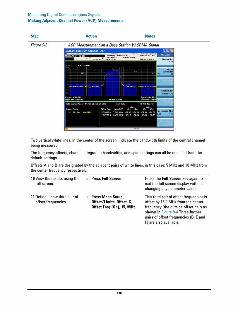
116
Measuring Digital Communications SignalsMaking Adjacent Channel Power (ACP) Measurements
Figure 9-3 ACP Measurement on a Base Station W-CDMA Signal
Two vertical white lines, in the center of the screen, indicate the bandwidth limits of the central channel being measured.The frequency offsets, channel integration bandwidths, and span settings can all be modified from the default settings.Offsets A and B are designated by the adjacent pairs of white lines, in this case: 5 MHz and 10 MHz from the center frequency respectively.
10 View the results using the full screen.
a. Press Full Screen. Press the Full Screen key again to exit the full screen display without changing any parameter values.
11 Define a new third pair of offset frequencies.
a. Press Meas Setup, Offset/Limits, Offset, C, Offset Freq (On), 15, MHz.
This third pair of offset frequencies is offset by 15.0 MHz from the center frequency (the outside offset pair) as shown in Figure 9-4 Three further pairs of offset frequencies (D, E and F) are also available.
Step Action Notes
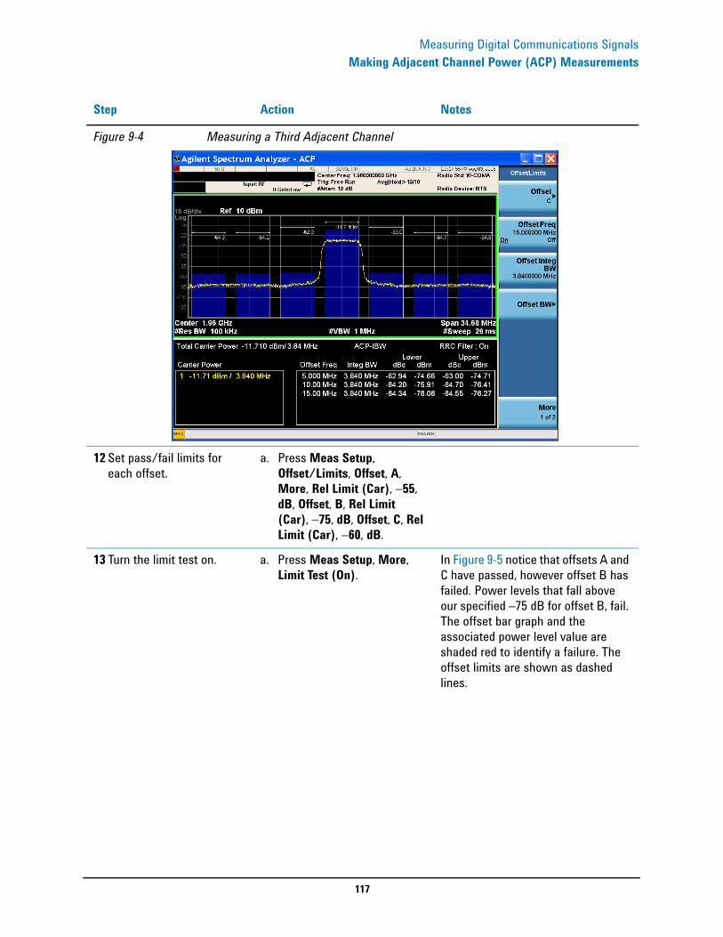
117
Measuring Digital Communications SignalsMaking Adjacent Channel Power (ACP) Measurements
Figure 9-4 Measuring a Third Adjacent Channel
12 Set pass/fail limits for each offset.
a. Press Meas Setup, Offset/Limits, Offset, A, More, Rel Limit (Car), −55, dB, Offset, B, Rel Limit (Car), −75, dB, Offset, C, Rel Limit (Car), −60, dB.
13 Turn the limit test on. a. Press Meas Setup, More, Limit Test (On).
In Figure 9-5 notice that offsets A and C have passed, however offset B has failed. Power levels that fall above our specified –75 dB for offset B, fail. The offset bar graph and the associated power level value are shaded red to identify a failure. The offset limits are shown as dashed lines.
Step Action Notes
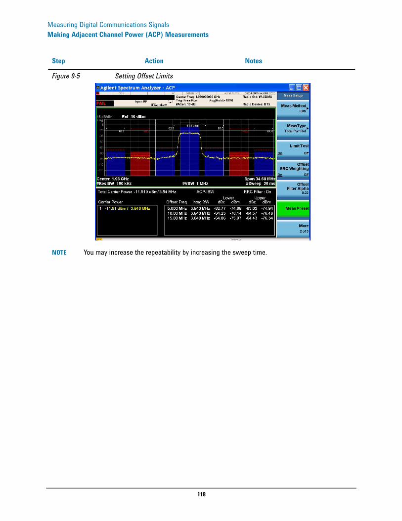
118
Measuring Digital Communications SignalsMaking Adjacent Channel Power (ACP) Measurements
Figure 9-5 Setting Offset Limits
NOTE You may increase the repeatability by increasing the sweep time.
Step Action Notes
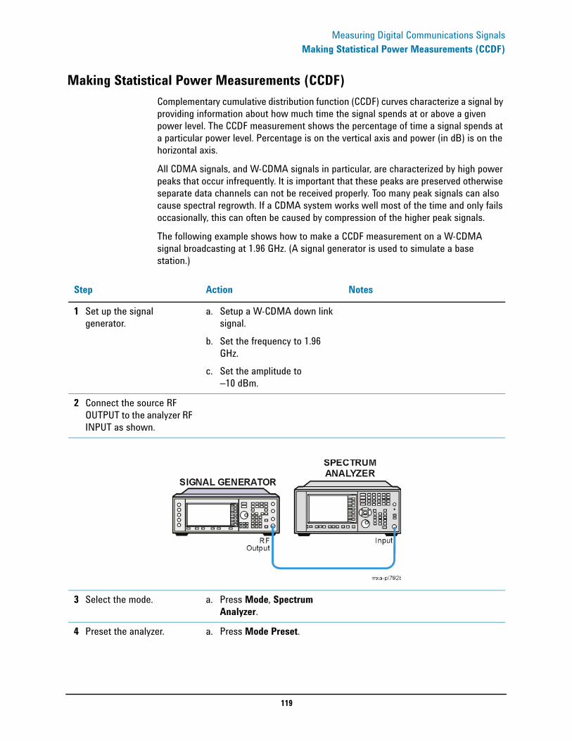
119
Measuring Digital Communications SignalsMaking Statistical Power Measurements (CCDF)
Making Statistical Power Measurements (CCDF)Complementary cumulative distribution function (CCDF) curves characterize a signal by providing information about how much time the signal spends at or above a given power level. The CCDF measurement shows the percentage of time a signal spends at a particular power level. Percentage is on the vertical axis and power (in dB) is on the horizontal axis.
All CDMA signals, and W-CDMA signals in particular, are characterized by high power peaks that occur infrequently. It is important that these peaks are preserved otherwise separate data channels can not be received properly. Too many peak signals can also cause spectral regrowth. If a CDMA system works well most of the time and only fails occasionally, this can often be caused by compression of the higher peak signals.
The following example shows how to make a CCDF measurement on a W-CDMA signal broadcasting at 1.96 GHz. (A signal generator is used to simulate a base station.)
Step Action Notes
1 Set up the signal generator.
a. Setup a W-CDMA down link signal.
b. Set the frequency to 1.96 GHz.
c. Set the amplitude to −10 dBm.
2 Connect the source RF OUTPUT to the analyzer RF INPUT as shown.
3 Select the mode. a. Press Mode, Spectrum Analyzer.
4 Preset the analyzer. a. Press Mode Preset.
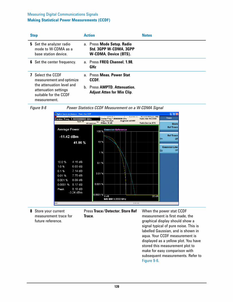
120
Measuring Digital Communications SignalsMaking Statistical Power Measurements (CCDF)
5 Set the analyzer radio mode to W-CDMA as a base station device.
a. Press Mode Setup, Radio Std, 3GPP W-CDMA, 3GPP W-CDMA, Device (BTS).
6 Set the center frequency. a. Press FREQ Channel, 1.98, GHz
7 Select the CCDF measurement and optimize the attenuation level and attenuation settings suitable for the CCDF measurement.
a. Press Meas, Power Stat CCDF.
b. Press AMPTD, Attenuation, Adjust Atten for Min Clip.
Figure 9-6 Power Statistics CCDF Measurement on a W-CDMA Signal
8 Store your current measurement trace for future reference.
Press Trace/Detector, Store Ref Trace.
When the power stat CCDF measurement is first made, the graphical display should show a signal typical of pure noise. This is labelled Gaussian, and is shown in aqua. Your CCDF measurement is displayed as a yellow plot. You have stored this measurement plot to make for easy comparison with subsequent measurements. Refer to Figure 9-6.
Step Action Notes
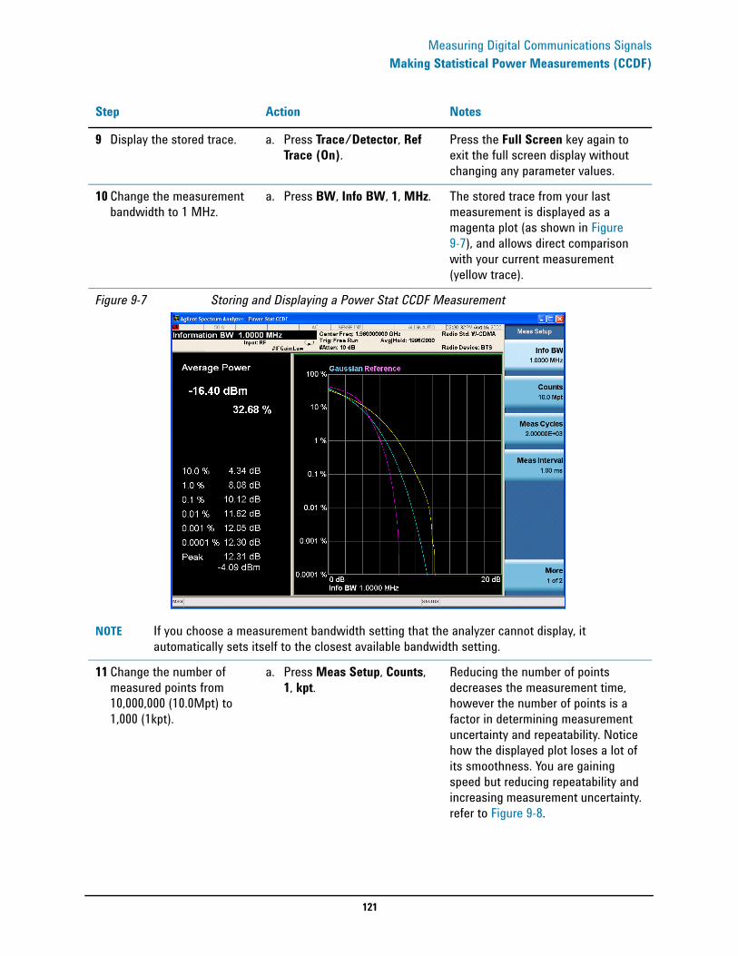
121
Measuring Digital Communications SignalsMaking Statistical Power Measurements (CCDF)
9 Display the stored trace. a. Press Trace/Detector, Ref Trace (On).
Press the Full Screen key again to exit the full screen display without changing any parameter values.
10 Change the measurement bandwidth to 1 MHz.
a. Press BW, Info BW, 1, MHz. The stored trace from your last measurement is displayed as a magenta plot (as shown in Figure 9-7), and allows direct comparison with your current measurement (yellow trace).
Figure 9-7 Storing and Displaying a Power Stat CCDF Measurement
NOTE If you choose a measurement bandwidth setting that the analyzer cannot display, it automatically sets itself to the closest available bandwidth setting.
11 Change the number of measured points from 10,000,000 (10.0Mpt) to 1,000 (1kpt).
a. Press Meas Setup, Counts, 1, kpt.
Reducing the number of points decreases the measurement time, however the number of points is a factor in determining measurement uncertainty and repeatability. Notice how the displayed plot loses a lot of its smoothness. You are gaining speed but reducing repeatability and increasing measurement uncertainty. refer to Figure 9-8.
Step Action Notes

122
Measuring Digital Communications SignalsMaking Statistical Power Measurements (CCDF)
Figure 9-8 Reducing the Measurement Points to 1 kpt
NOTE The number of points collected per sweep is dependent on the sampling rate and the measurement interval. The number of samples that have been processed are indicated at the top of the screen. The graphical plot is continuously updated so you can see it getting smoother as measurement uncertainty is reduced and repeatability improves.
12 Change the scaling of the X-axis to 1 dB per division to optimize your particular measurement.
a. Press SPAN X Scale, Scale/Div, 1, dB.
Refer to Figure 9-9.
Step Action Notes
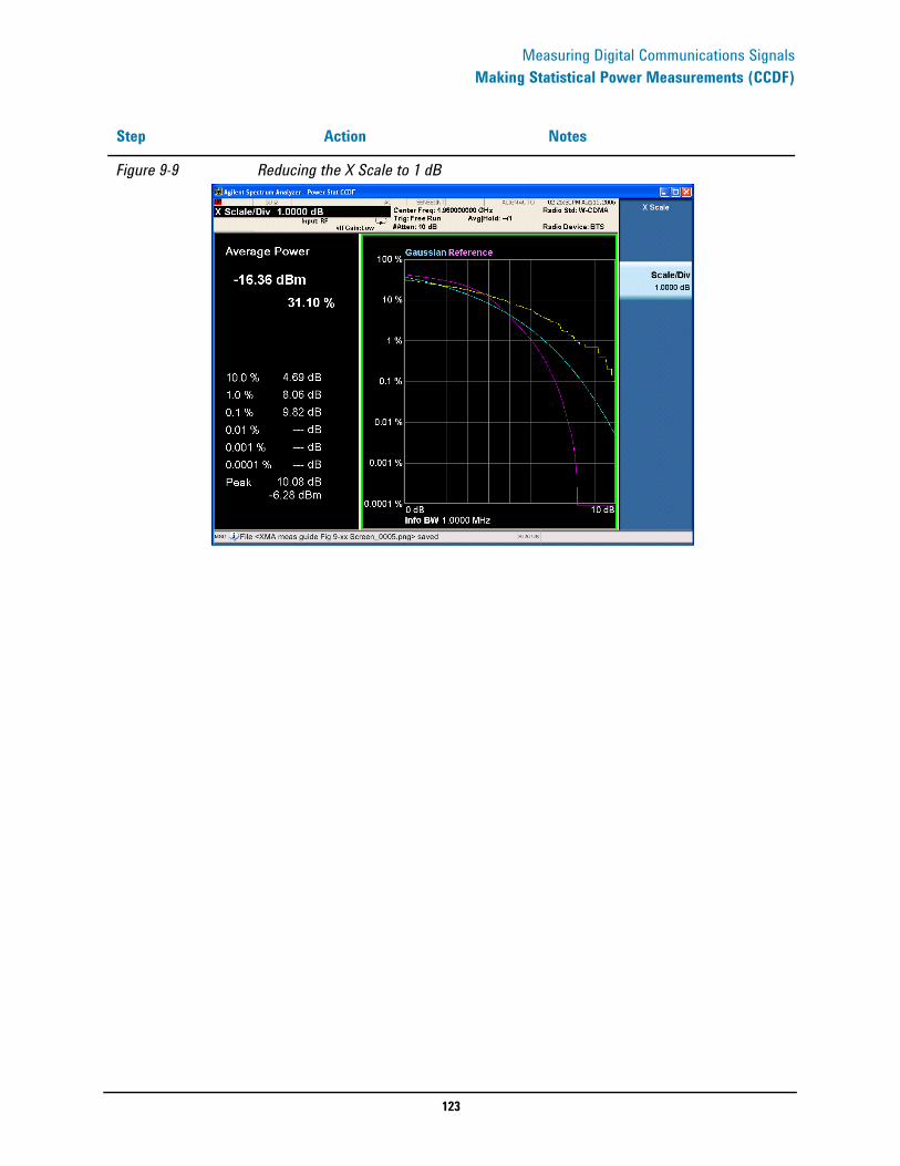
123
Measuring Digital Communications SignalsMaking Statistical Power Measurements (CCDF)
Figure 9-9 Reducing the X Scale to 1 dB
Step Action Notes
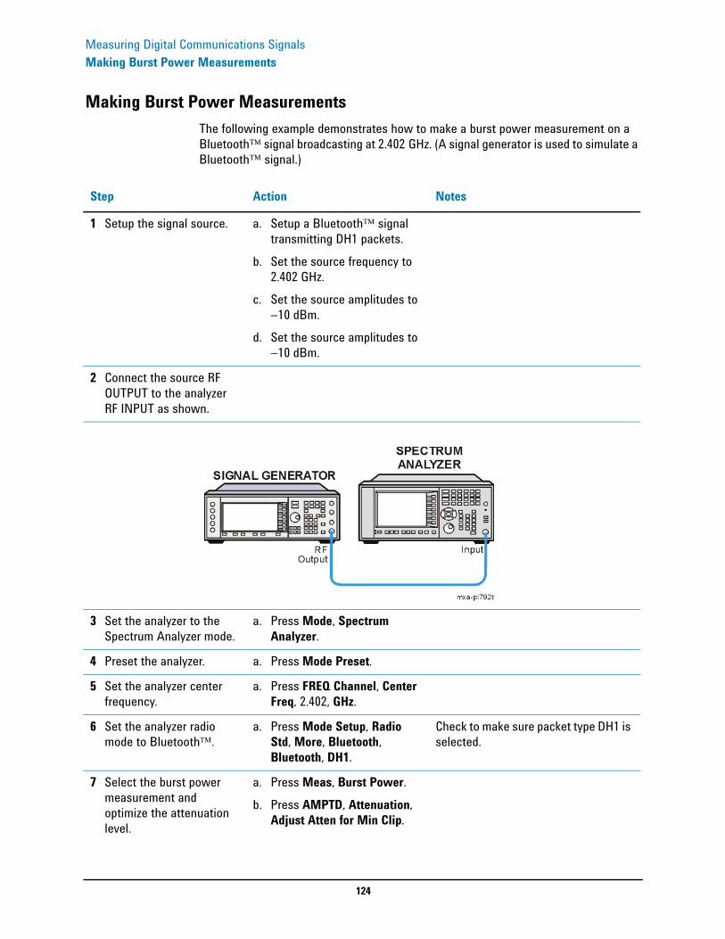
124
Measuring Digital Communications SignalsMaking Burst Power Measurements
Making Burst Power MeasurementsThe following example demonstrates how to make a burst power measurement on a Bluetooth™ signal broadcasting at 2.402 GHz. (A signal generator is used to simulate a Bluetooth™ signal.)
Step Action Notes
1 Setup the signal source. a. Setup a Bluetooth™ signal transmitting DH1 packets.
b. Set the source frequency to 2.402 GHz.
c. Set the source amplitudes to −10 dBm.
d. Set the source amplitudes to −10 dBm.
2 Connect the source RF OUTPUT to the analyzer RF INPUT as shown.
3 Set the analyzer to the Spectrum Analyzer mode.
a. Press Mode, Spectrum Analyzer.
4 Preset the analyzer. a. Press Mode Preset.
5 Set the analyzer center frequency.
a. Press FREQ Channel, Center Freq, 2.402, GHz.
6 Set the analyzer radio mode to Bluetooth™.
a. Press Mode Setup, Radio Std, More, Bluetooth, Bluetooth, DH1.
Check to make sure packet type DH1 is selected.
7 Select the burst power measurement and optimize the attenuation level.
a. Press Meas, Burst Power.b. Press AMPTD, Attenuation,
Adjust Atten for Min Clip.

125
Measuring Digital Communications SignalsMaking Burst Power Measurements
8 View the results of the burst power measurement using the full screen).
a. Press Full Screen. See Figure 9-10.
Figure 9-10 Full Screen Display of Burst Power Measurement Results
NOTE Press the Full Screen key again to exit the full screen display without changing any parameter values. Refer to Figure 9-11
Step Action Notes
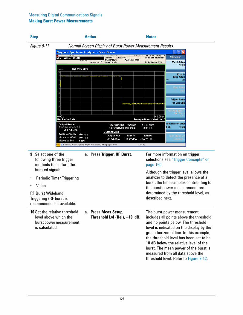
126
Measuring Digital Communications SignalsMaking Burst Power Measurements
Figure 9-11 Normal Screen Display of Burst Power Measurement Results
9 Select one of the following three trigger methods to capture the bursted signal:
• Periodic Timer Triggering• VideoRF Burst Wideband Triggering (RF burst is recommended, if available.
a. Press Trigger, RF Burst. For more information on trigger selections see “Trigger Concepts” on page 160.Although the trigger level allows the analyzer to detect the presence of a burst, the time samples contributing to the burst power measurement are determined by the threshold level, as described next.
10 Set the relative threshold level above which the burst power measurement is calculated.
a. Press Meas Setup, Threshold Lvl (Rel), −10, dB.
The burst power measurement includes all points above the threshold and no points below. The threshold level is indicated on the display by the green horizontal line. In this example, the threshold level has been set to be 10 dB below the relative level of the burst. The mean power of the burst is measured from all data above the threshold level. Refer to Figure 9-12.
Step Action Notes
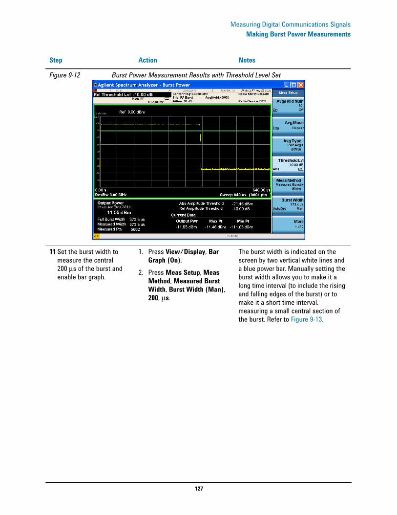
127
Measuring Digital Communications SignalsMaking Burst Power Measurements
Figure 9-12 Burst Power Measurement Results with Threshold Level Set
11 Set the burst width to measure the central 200 μs of the burst and enable bar graph.
1. Press View/Display, Bar Graph (On).
2. Press Meas Setup, Meas Method, Measured Burst Width, Burst Width (Man), 200, μs.
The burst width is indicated on the screen by two vertical white lines and a blue power bar. Manually setting the burst width allows you to make it a long time interval (to include the rising and falling edges of the burst) or to make it a short time interval, measuring a small central section of the burst. Refer to Figure 9-13.
Step Action Notes

128
Measuring Digital Communications SignalsMaking Burst Power Measurements
Figure 9-13 Bar Graph Results with Measured Burst Width Set
NOTE If you set the burst width manually to be wider than the screen's display, the vertical white lines move off the edges of the screen. This could give misleading results as only the data on the screen can be measured.The Bluetooth™ standard states that power measurements should be taken over at least 20% to 80% of the duration of the burst.
12 Increase the sweep time to display more than one burst at a time.
Press Sweep/Control, Sweep Time, 6200, μs (or 6.2, ms).
The screen display shows several bursts in a single sweep as in Figure 9-14. The burst power measurement measures the mean power of the first burst, indicated by the vertical white lines and blue power bar.
Step Action Notes
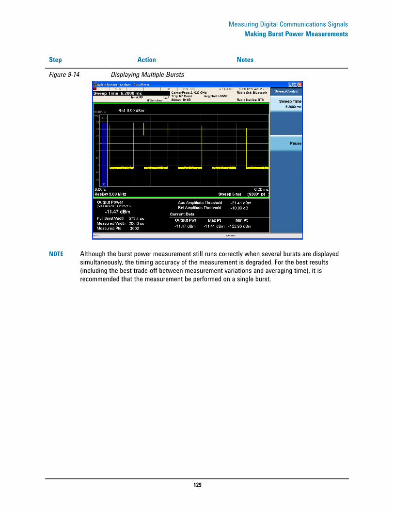
129
Measuring Digital Communications SignalsMaking Burst Power Measurements
Figure 9-14 Displaying Multiple Bursts
NOTE Although the burst power measurement still runs correctly when several bursts are displayed simultaneously, the timing accuracy of the measurement is degraded. For the best results (including the best trade-off between measurement variations and averaging time), it is recommended that the measurement be performed on a single burst.
Step Action Notes

130
Measuring Digital Communications SignalsSpurious Emissions Measurements
Spurious Emissions MeasurementsThe following example demonstrates how to make a spurious emissions measurement on a multitone signal used to simulate a spurious emission in a measured spectrum.
Step Action Notes
1 Setup the signal source. a. Setup a multitone signal with 8 tones with a 2.0 MHz frequency spacing.
b. Set the source frequency to 1.950 GHz.
c. Set the source amplitudes to −50 dBm.
2 Connect the source RF OUTPUT to the analyzer RF INPUT as shown.
3 Set the analyzer to the Spectrum Analyzer mode.
a. Press Mode, Spectrum Analyzer.
4 Preset the analyzer. a. Press Mode Preset.
5 Set the analyzer center frequency.
a. Press FREQ Channel, Center Freq, 1.950, GHz.
6 Select the spurious emissions measurement.
a. Press Meas, More, Spurious Emissions.

131
Measuring Digital Communications SignalsSpurious Emissions Measurements
7 You may Focus the display on a specific spurious emissions signal.
a. Press Meas Setup, Spur, 1, Enter (or enter the number of the spur of interest)
b. Press Meas Type to highlight Examine
The Spurious Emission result should look like Figure 9-15. The graph window and a text window are displayed. The text window shows the list of detected spurs. Each line item includes the spur number, the range in which the spur was detected, the power of the spur, and the limit value against which the spur amplitude is tested.
Figure 9-15 Spurious Emission Measurement Result
8 You may customize the tested ranges for spurious emissions (initially 5 default ranges and parameters are loaded into the range table).
a. Press Meas Setup, Range Table, then select and edit the available parameters.
Step Action Notes
132
Measuring Digital Communications SignalsSpurious Emissions Measurements
Troubleshooting HintsSpurious emissions measurements can reveal the presence of degraded or defective parts in the transmitter section of the UUT. The following are examples of problems which, once indicated by testing, may require further attention:
• Faulty DC power supply control of the transmitter power amplifier• RF power controller of the pre-power amplifier stage• I/Q control of the baseband stage• Reduction in the gain and output power level of the amplifier due to a degraded
gain control and/or increased distortion• Degradation of amplifier linearity and other performance characteristicsPower amplifiers are one of the final stage elements of a base transmitter and play a critical part in meeting the important power and spectral efficiency specifications. Measuring the spectral response of these amplifiers to complex wideband signals is crucial to linking amplifier linearity and other performance characteristics to the stringent system specifications.

133
Measuring Digital Communications SignalsSpectrum Emission Mask Measurements
Spectrum Emission Mask MeasurementsThis section explains how to make the spectrum emission mask measurement on a W-CDMA (3GPP) mobile station. (A signal generator is used to simulate a mobile station.) SEM compares the total power level within the defined carrier bandwidth and the given offset channels on both sides of the carrier frequency, to levels allowed by the standard. Results of the measurement of each offset segment can be viewed separately.
Step Action Notes
1 Setup the signal source. a. Setup a W-CDMA uplink signal.
b. Set the source frequency to 1,920 MHz (Channel. Number: 5 × 1,920 = 9,600).
c. Set the source amplitudes to 0 dBm.
2 Connect the source RF OUTPUT to the analyzer RF INPUT as shown.
3 Select the mode. a. Press Mode, Spectrum Analyzer.
4 Preset the analyzer. a. Press Mode Preset.
5 Set the radio standard and toggle the device to mobile station.
a. Press Mode Setup, Radio Std, 3GPP W-CDMA, 3GPP W-CDMA, Device (MS).
6 Set the center frequency. a. Press FREQ Channel, 1.920, GHz.
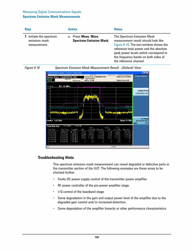
134
Measuring Digital Communications SignalsSpectrum Emission Mask Measurements
Troubleshooting HintsThis spectrum emission mask measurement can reveal degraded or defective parts in the transmitter section of the UUT. The following examples are those areas to be checked further.
• Faulty DC power supply control of the transmitter power amplifier.
• RF power controller of the pre-power amplifier stage.
• I/Q control of the baseband stage.
• Some degradation in the gain and output power level of the amplifier due to the degraded gain control and/or increased distortion.
• Some degradation of the amplifier linearity or other performance characteristics.
7 Initiate the spectrum emission mask measurement.
a. Press Meas, More, Spectrum Emission Mask.
The Spectrum Emission Mask measurement result should look like Figure 9-16. The text window shows the reference total power and the absolute peak power levels which correspond to the frequency bands on both sides of the reference channel.
Figure 9-16 Spectrum Emission Mask Measurement Result - (Default) View
Step Action Notes
135
Measuring Digital Communications SignalsSpectrum Emission Mask Measurements
Power amplifiers are one of the final stage elements of a base or mobile transmitter and are a critical part of meeting the important power and spectral efficiency specifications. Since spectrum emission mask measures the spectral response of the amplifier to a complex wideband signal, it is a key measurement linking amplifier linearity and other performance characteristics to the stringent system specifications.

136
Measuring Digital Communications SignalsSpectrum Emission Mask Measurements

137
Demodulating AM Signals
10 Demodulating AM Signals
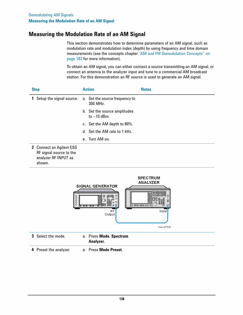
138
Demodulating AM SignalsMeasuring the Modulation Rate of an AM Signal
Measuring the Modulation Rate of an AM Signal This section demonstrates how to determine parameters of an AM signal, such as modulation rate and modulation index (depth) by using frequency and time domain measurements (see the concepts chapter “AM and FM Demodulation Concepts” on page 182 for more information).
To obtain an AM signal, you can either connect a source transmitting an AM signal, or connect an antenna to the analyzer input and tune to a commercial AM broadcast station. For this demonstration an RF source is used to generate an AM signal.
Step Action Notes
1 Setup the signal source. a. Set the source frequency to 300 MHz.
b. Set the source amplitudes to −10 dBm.
c. Set the AM depth to 80%.d. Set the AM rate to 1 kHz.e. Turn AM on.
2 Connect an Agilent ESG RF signal source to the analyzer RF INPUT as shown.
3 Select the mode. a. Press Mode, Spectrum Analyzer.
4 Preset the analyzer. a. Press Mode Preset.
139
Demodulating AM SignalsMeasuring the Modulation Rate of an AM Signal
5 Set the center frequency, span, RBW and the sweep time.
a. Press FREQ Channel, Center Freq, 300, MHz.
b. Press SPAN X Scale, Span, 500, kHz.
c. Press BW, Res BW, 30, kHz.
d. Press Sweep/Control, Sweep Time, 20, ms.
6 Change the y-scale type to linear.
a. Press AMPTD Y Scale, Scale Type (Lin).
The y-axis units will automatically set to volts.
7 Position the signal peak near the first graticule below the reference level.
a. Press AMPTD Y Scale, Ref Level, (rotate front-panel knob).
8 Set the analyzer in zero span to make time-domain measurements
a. Press SPAN X Scale, Zero Span
b. Press Sweep/Control, Sweep Time, 5, ms
9 Use the video trigger to stabilize the trace.
a. Press Trigger, Video. Since the modulation is a steady tone, you can use video trigger to trigger the analyzer sweep on the waveform and stabilize the trace, much like an oscilloscope. See Figure 10-1If the trigger level is set too high or too low when video trigger mode is activated, the sweep stops. You need to adjust the trigger level up or down with the front-panel knob until the sweep begins again.
10 Measure the AM rate using delta markers.
a. Press Peak Search, Marker Delta, Next Right or Next Left.
Use markers and delta markers to measure the AM rate. Place the marker on a peak and then use a delta marker to measure the time difference between the peaks (this is the AM rate of the signal)
Step Action Notes
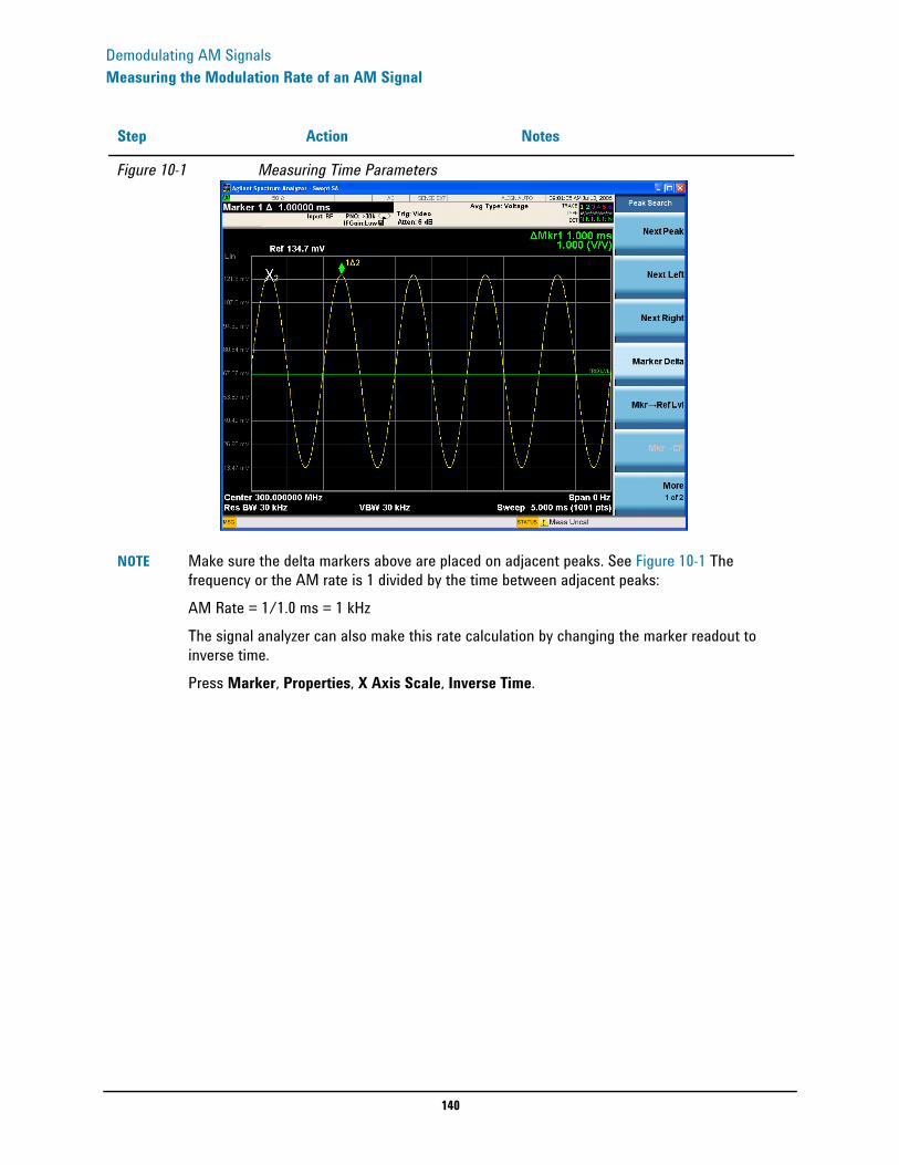
140
Demodulating AM SignalsMeasuring the Modulation Rate of an AM Signal
Figure 10-1 Measuring Time Parameters
NOTE Make sure the delta markers above are placed on adjacent peaks. See Figure 10-1 The frequency or the AM rate is 1 divided by the time between adjacent peaks:AM Rate = 1/1.0 ms = 1 kHzThe signal analyzer can also make this rate calculation by changing the marker readout to inverse time.Press Marker, Properties, X Axis Scale, Inverse Time.
Step Action Notes

141
Demodulating AM SignalsMeasuring the Modulation Rate of an AM Signal
Figure 10-2 Measuring Time Parameters with Inverse Time Readout
Another way to calculate the modulation rate would be to view the signal in the frequency domain and measure the delta frequency between the peak of the carrier and the first sideband.
Step Action Notes
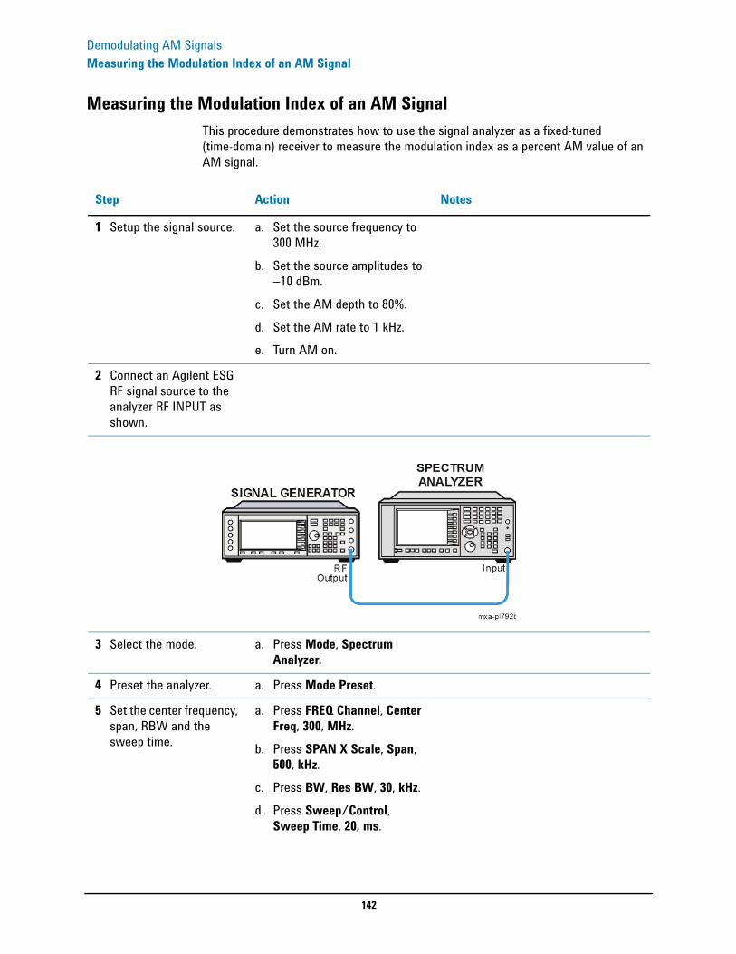
142
Demodulating AM SignalsMeasuring the Modulation Index of an AM Signal
Measuring the Modulation Index of an AM SignalThis procedure demonstrates how to use the signal analyzer as a fixed-tuned (time-domain) receiver to measure the modulation index as a percent AM value of an AM signal.
Step Action Notes
1 Setup the signal source. a. Set the source frequency to 300 MHz.
b. Set the source amplitudes to −10 dBm.
c. Set the AM depth to 80%.d. Set the AM rate to 1 kHz.e. Turn AM on.
2 Connect an Agilent ESG RF signal source to the analyzer RF INPUT as shown.
3 Select the mode. a. Press Mode, Spectrum Analyzer.
4 Preset the analyzer. a. Press Mode Preset.
5 Set the center frequency, span, RBW and the sweep time.
a. Press FREQ Channel, Center Freq, 300, MHz.
b. Press SPAN X Scale, Span, 500, kHz.
c. Press BW, Res BW, 30, kHz.d. Press Sweep/Control,
Sweep Time, 20, ms.
143
Demodulating AM SignalsMeasuring the Modulation Index of an AM Signal
6 Set the y-axis units to volts.
a. Press AMPTD Y Scale, More, Y-Axis Units, V (Volts).
7 Position the signal peak near the reference level.
a. Press AMPTD Y Scale, Ref Level, (rotate front-panel knob).
8 Change the y-scale type to linear.
a. Press AMPTD Y Scale, Scale Type (Lin).
9 Set the analyzer in zero span to make time-domain measurements.
a. Press SPAN X Scale, Zero Span.
b. Press Sweep/Control, Sweep Time, 5, ms
10 Place the analyzer in free run trigger mode.
a. Press Trigger, Free Run.
11 Increase the sweep time and decrease the VBW.
a. Press Sweep/Control, Sweep Time, 5, s.
b. Press BW, Video BW, 30, Hz.
The waveform is displayed as a flat horizontal signal.
12 Center the flat waveform at the mid-point of the y-axis and then widen the VBW and decrease the sweep time to display the waveform as a sine wave.
a. Press AMPTD Y Scale, Ref Level, (rotate front-panel knob).
b. Press BW, Video BW, 100, kHz.
c. Press Sweep/Control, Sweep Time, 5, ms.
13 Measure the modulation index of the AM signal.
To measure the modulation index as % AM, read the trace as follows (see Figure 10-3 for display examples): 100% AM extends from the top graticule down to the bottom graticule. 80% AM (as in this example) is when the top of the signal is at 1 division below the top graticule and 1 division above the bottom graticule. To determine % AM of your signal count each y-axis division as 10%.
Step Action Notes

144
Demodulating AM SignalsMeasuring the Modulation Index of an AM Signal
Figure 10-3 AM Signal Measured in the Time Domain
LEFT: 100% AM Signal (Modulation Index = 1) RIGHT: 80% AM Signal (Modulation Index = 0.8)
Step Action Notes

145
IQ Analyzer Measurement
11 IQ Analyzer Measurement

146
IQ Analyzer MeasurementCapturing wideband signals for further analysis
Capturing wideband signals for further analysisThis section demonstrates how to capture complex time domain data from wide bandwidth RF signals. This mode preserves the instantaneous vector relationships of time, frequency, phase and amplitude contained within the selected digitizer span or analysis BW, at the analyzer's center frequency, for output as IQ data. This IQ data can then be utilized internally or output over LAN, USB or GPIB for use with external analysis tools. Each measurement description specifies the types of data available remotely for that measurement.
The standard 10 MHz Analysis BW and optional 25 MHz Analysis BW digitizers used to capture the wide bandwidth RF signals can be accessed from the front panel in IQ Analyzer (Basic) mode. This IQ Analyzer mode provides basic setup, RF (FFT based) and IQ analysis tools
Within the IQ Analyzer mode, basic frequency domain, time domain and IQ measurements are available as initial signal and data verification tools in preparation for deriving the IQ data output.
The Complex Spectrum measurement provides a display in the upper window of power versus frequency with current (yellow trace) and average (blue trace) data. In addition, an IQ waveform of voltage versus time is provided in the lower window.
The IQ Waveform measurement provides a time domain view of the RF signal envelope with power versus time or an IQ waveform of voltage versus time.
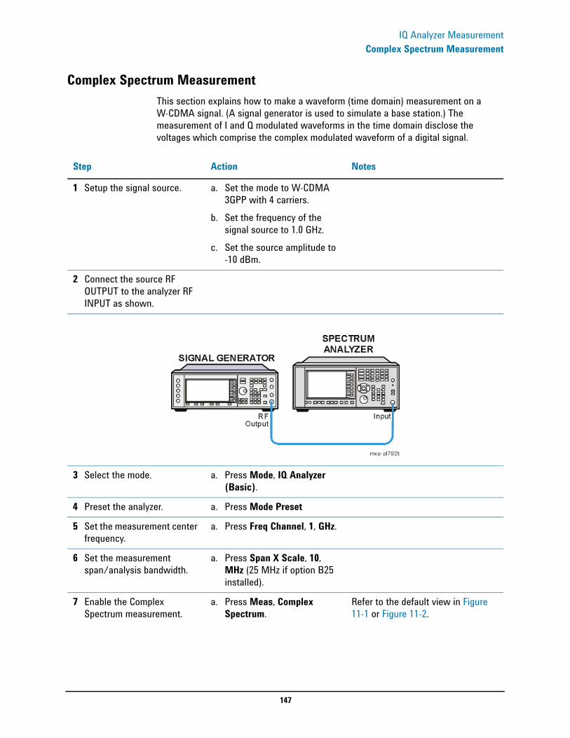
147
IQ Analyzer MeasurementComplex Spectrum Measurement
Complex Spectrum MeasurementThis section explains how to make a waveform (time domain) measurement on a W-CDMA signal. (A signal generator is used to simulate a base station.) The measurement of I and Q modulated waveforms in the time domain disclose the voltages which comprise the complex modulated waveform of a digital signal.
Step Action Notes
1 Setup the signal source. a. Set the mode to W-CDMA 3GPP with 4 carriers.
b. Set the frequency of the signal source to 1.0 GHz.
c. Set the source amplitude to -10 dBm.
2 Connect the source RF OUTPUT to the analyzer RF INPUT as shown.
3 Select the mode. a. Press Mode, IQ Analyzer (Basic).
4 Preset the analyzer. a. Press Mode Preset
5 Set the measurement center frequency.
a. Press Freq Channel, 1, GHz.
6 Set the measurement span/analysis bandwidth.
a. Press Span X Scale, 10, MHz (25 MHz if option B25 installed).
7 Enable the Complex Spectrum measurement.
a. Press Meas, Complex Spectrum.
Refer to the default view in Figure 11-1 or Figure 11-2.
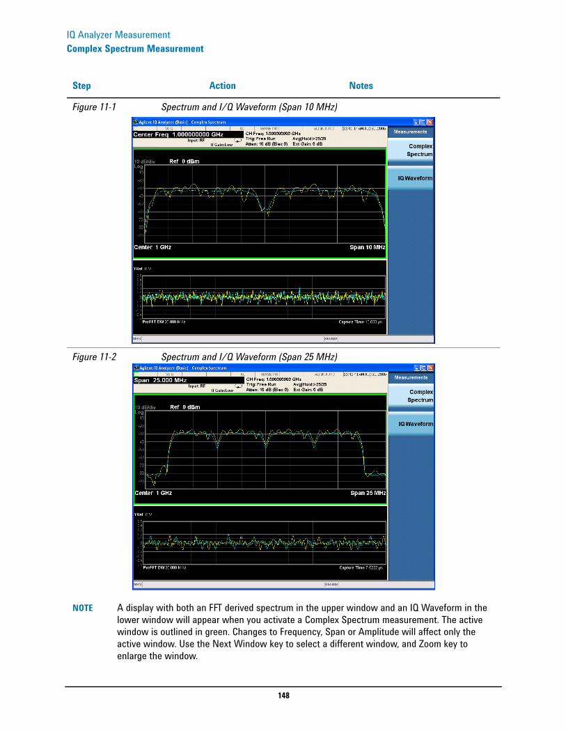
148
IQ Analyzer MeasurementComplex Spectrum Measurement
Figure 11-1 Spectrum and I/Q Waveform (Span 10 MHz)
Figure 11-2 Spectrum and I/Q Waveform (Span 25 MHz)
NOTE A display with both an FFT derived spectrum in the upper window and an IQ Waveform in the lower window will appear when you activate a Complex Spectrum measurement. The active window is outlined in green. Changes to Frequency, Span or Amplitude will affect only the active window. Use the Next Window key to select a different window, and Zoom key to enlarge the window.
Step Action Notes
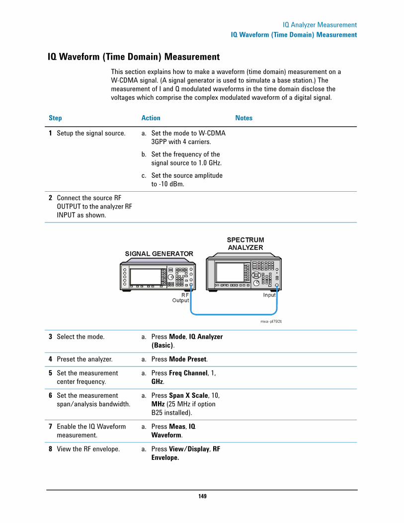
149
IQ Analyzer MeasurementIQ Waveform (Time Domain) Measurement
IQ Waveform (Time Domain) MeasurementThis section explains how to make a waveform (time domain) measurement on a W-CDMA signal. (A signal generator is used to simulate a base station.) The measurement of I and Q modulated waveforms in the time domain disclose the voltages which comprise the complex modulated waveform of a digital signal.
Step Action Notes
1 Setup the signal source. a. Set the mode to W-CDMA 3GPP with 4 carriers.
b. Set the frequency of the signal source to 1.0 GHz.
c. Set the source amplitude to -10 dBm.
2 Connect the source RF OUTPUT to the analyzer RF INPUT as shown.
3 Select the mode. a. Press Mode, IQ Analyzer (Basic).
4 Preset the analyzer. a. Press Mode Preset.
5 Set the measurement center frequency.
a. Press Freq Channel, 1, GHz.
6 Set the measurement span/analysis bandwidth.
a. Press Span X Scale, 10, MHz (25 MHz if option B25 installed).
7 Enable the IQ Waveform measurement.
a. Press Meas, IQ Waveform.
8 View the RF envelope. a. Press View/Display, RF Envelope.

150
IQ Analyzer MeasurementIQ Waveform (Time Domain) Measurement
9 Set the analysis bandwidth.
a. Press BW, Info BW, 10, MHz (25 MHz if option B25 installed).
This view provides a waveform display of power versus time of the RF signal in the upper window with metrics for mean and peak-to-mean in the lower window. Refer to Figure 11-3 or Figure 11-4.
Figure 11-3 IQ Waveform Measurement - Time domain View (10 MHz BW)
Figure 11-4 IQ Waveform Measurement - Time domain View (25 MHz BW)
Step Action Notes
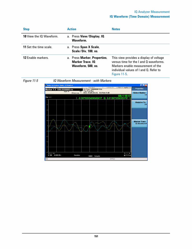
151
IQ Analyzer MeasurementIQ Waveform (Time Domain) Measurement
10 View the IQ Waveform. a. Press View/Display, IQ Waveform.
11 Set the time scale. a. Press Span X Scale, Scale/Div, 100, ns.
12 Enable markers. a. Press Marker, Properties, Marker Trace, IQ Waveform, 500, ns.
This view provides a display of voltage versus time for the I and Q waveforms. Markers enable measurement of the individual values of I and Q. Refer to Figure 11-5.
Figure 11-5 IQ Waveform Measurement - with Markers
Step Action Notes

152
IQ Analyzer MeasurementIQ Waveform (Time Domain) Measurement
153
Using Option BBA Baseband I/Q Inputs
12 Using Option BBA Baseband I/Q Inputs
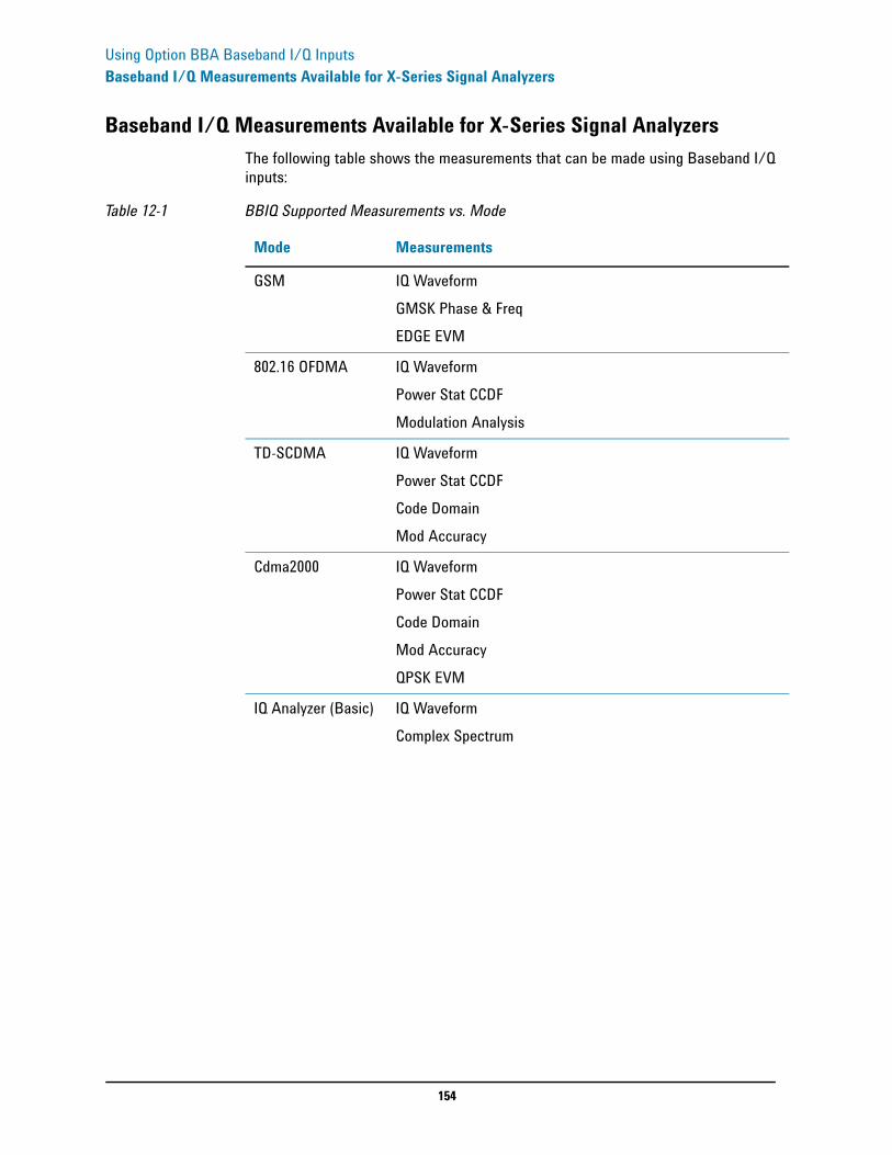
154
Using Option BBA Baseband I/Q InputsBaseband I/Q Measurements Available for X-Series Signal Analyzers
Baseband I/Q Measurements Available for X-Series Signal AnalyzersThe following table shows the measurements that can be made using Baseband I/Q inputs:
Table 12-1 BBIQ Supported Measurements vs. Mode
Mode Measurements
GSM IQ WaveformGMSK Phase & FreqEDGE EVM
802.16 OFDMA IQ WaveformPower Stat CCDFModulation Analysis
TD-SCDMA IQ WaveformPower Stat CCDFCode DomainMod Accuracy
Cdma2000 IQ WaveformPower Stat CCDFCode DomainMod AccuracyQPSK EVM
IQ Analyzer (Basic) IQ WaveformComplex Spectrum
155
Using Option BBA Baseband I/Q InputsBaseband I/Q Measurement Overview
Baseband I/Q Measurement OverviewThe Baseband I/Q functionality is a hardware option, Option BBA. If the option is not installed in the instrument, the I/Q functionality cannot be enabled.
The Baseband I/Q option provides four input ports and one Calibration Output port. The input ports are I, I-bar, Q, and Q-bar. The I and I-bar together compose the I channel and the Q and Q-bar together compose the Q channel. Each channel has two modes of operation:
The system supports a variety of input passive probes as well as the Agilent 1153A active differential probe using the infinimax probe interface.
NOTE To avoid duplication, this section describes only the details unique to using the baseband I/Q inputs. For generic measurement details, refer to the previous “Making Measurements” sections.
To make measurements using baseband I/Q Inputs, make the following selections:
Mode Description
Single Ended(unbalanced)
In this mode, only the main port (I or Q) is used and the complementary ports (I-bar or Q-bar) is ignored. The I and Q ports are in single-ended mode when Differential “Off” is selected.
Differential(balanced)
In this mode, both main and complementary ports are used. To activate this mode, select Differential “On” from the I and Q Setup softkey menus.
Step Notes
Select measurement. Select a measurement that supports baseband I/Q inputs.
Select the I/Q Path. Press Input/Output, I/Q, I/Q Path.Select from the choices present on the screen. The path selected is shown at the top of the measurement screen.
Select the appropriate circuit location and probe(s) for measurements.
For details see ““Selecting Input Probes for Baseband Measurements” on page 190” in the Concepts chapter.
Select baseband I/Q input connectors.
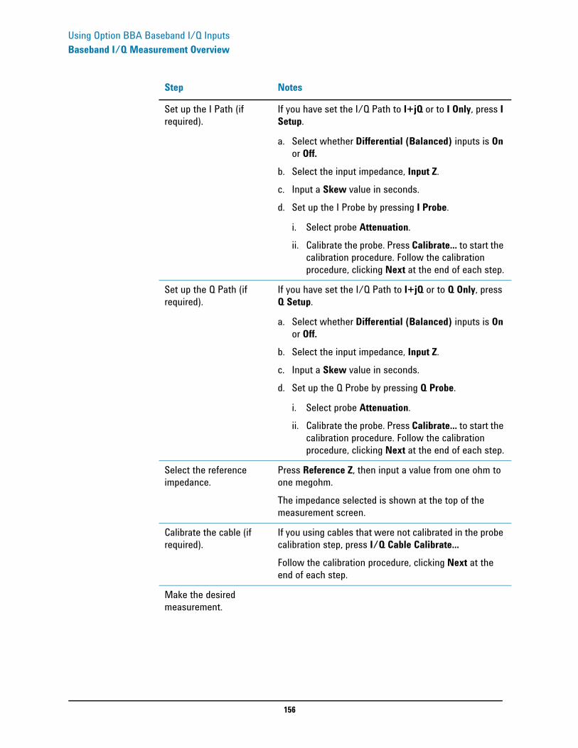
156
Using Option BBA Baseband I/Q InputsBaseband I/Q Measurement Overview
Set up the I Path (if required).
If you have set the I/Q Path to I+jQ or to I Only, press I Setup.
a. Select whether Differential (Balanced) inputs is On or Off.
b. Select the input impedance, Input Z.c. Input a Skew value in seconds.d. Set up the I Probe by pressing I Probe.
i. Select probe Attenuation.ii. Calibrate the probe. Press Calibrate... to start the
calibration procedure. Follow the calibration procedure, clicking Next at the end of each step.
Set up the Q Path (if required).
If you have set the I/Q Path to I+jQ or to Q Only, press Q Setup.
a. Select whether Differential (Balanced) inputs is On or Off.
b. Select the input impedance, Input Z.c. Input a Skew value in seconds.d. Set up the Q Probe by pressing Q Probe.
i. Select probe Attenuation.ii. Calibrate the probe. Press Calibrate... to start the
calibration procedure. Follow the calibration procedure, clicking Next at the end of each step.
Select the reference impedance.
Press Reference Z, then input a value from one ohm to one megohm.The impedance selected is shown at the top of the measurement screen.
Calibrate the cable (if required).
If you using cables that were not calibrated in the probe calibration step, press I/Q Cable Calibrate... Follow the calibration procedure, clicking Next at the end of each step.
Make the desired measurement.
Step Notes
157
Concepts
13 Concepts
158
ConceptsResolving Closely Spaced Signals
Resolving Closely Spaced Signals
Resolving Signals of Equal AmplitudeTwo equal-amplitude input signals that are close in frequency can appear as a single signal trace on the analyzer display. Responding to a single-frequency signal, a swept-tuned analyzer traces out the shape of the selected internal IF (intermediate frequency) filter (typically referred to as the resolution bandwidth or RBW filter). As you change the filter bandwidth, you change the width of the displayed response. If a wide filter is used and two equal-amplitude input signals are close enough in frequency, then the two signals will appear as one signal. If a narrow enough filter is used, the two input signals can be discriminated and appear as separate peaks. Thus, signal resolution is determined by the IF filters inside the analyzer.
The bandwidth of the IF filter tells us how close together equal amplitude signals can be and still be distinguished from each other. The resolution bandwidth function selects an IF filter setting for a measurement. Typically, resolution bandwidth is defined as the 3 dB bandwidth of the filter. However, resolution bandwidth may also be defined as the 6 dB or impulse bandwidth of the filter.
Generally, to resolve two signals of equal amplitude, the resolution bandwidth must be less than or equal to the frequency separation of the two signals. If the bandwidth is equal to the separation and the video bandwidth is less than the resolution bandwidth, a dip of approximately 3 dB is seen between the peaks of the two equal signals, and it is clear that more than one signal is present.
For Signal Analyzers in swept mode, sweep time is automatically set to a value that is inversely proportional to the square of the resolution bandwidth (1/BW2),to keep the analyzer measurement calibrated. So, if the resolution bandwidth is reduced by a factor of 10, the sweep time is increased by a factor of 100 when sweep time and bandwidth settings are coupled. For the shortest measurement times, use the widest resolution bandwidth that still permits discrimination of all desired signals. Sweep time is also a function of which detector is in use, peak and normal detectors sweep as fast or more quickly than sample or average detectors. The analyzer allows RBW selections up to 8 MHz in 1, 3, 10 steps and it has the flexibility to fine tune RBWs in increments of 10% for a total of 160 RBW settings.
For best sweep times and keeping the analyzer calibrated set the sweep time (Sweep/Control, Sweep Time) to Auto, and the sweep type (Sweep/Control, Sweep Setup, Sweep Type) to Auto. Use the widest resolution bandwidth and the narrowest span that still permits resolution of all desired signals.
Resolving Small Signals Hidden by Large SignalsWhen dealing with the resolution of signals that are close together and not equal in amplitude, you must consider the shape of the IF filter of the analyzer, as well as its 3 dB bandwidth. (See “Resolving Signals of Equal Amplitude” on page 158 for more information.) The shape of a filter is defined by the selectivity, which is the ratio of the 60 dB bandwidth to the 3 dB bandwidth. If a small signal is too close to a larger signal, the smaller signal can be hidden by the skirt of the larger signal.
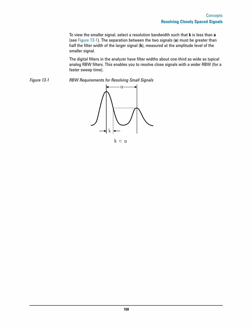
159
ConceptsResolving Closely Spaced Signals
To view the smaller signal, select a resolution bandwidth such that k is less than a (see Figure 13-1). The separation between the two signals (a) must be greater than half the filter width of the larger signal (k), measured at the amplitude level of the smaller signal.
The digital filters in the analyzer have filter widths about one-third as wide as typical analog RBW filters. This enables you to resolve close signals with a wider RBW (for a faster sweep time).
Figure 13-1 RBW Requirements for Resolving Small Signals
160
ConceptsTrigger Concepts
Trigger Concepts
NOTE The trigger functions let you select the trigger settings for a sweep or measurement. When using a trigger source other than Free Run, the analyzer will begin a sweep only with the selected trigger conditions are met. A trigger event is defined as the point at which your trigger source signal meets the specified trigger level and polarity requirements (if any). In FFT measurements, the trigger controls when the data is acquired for FFT conversion.
Selecting a Trigger1. Free Run Triggering
Pressing this key, when it is not selected, selects free-run triggering. Free run triggering occurs immediately after the sweep/measurement is initiated.
Press Trigger, Free Run
2. Video Triggering
The Video trigger condition is met when the video signal (the filtered and detected version of the input signal, including both RBW and VBW filtering) crosses the video trigger level. Video triggering triggers the measurement at the point at which the rising signal crosses the video trigger horizontal green line on the display:
Press Trigger, Video, Video, Trigger Level, −30, dBm. (If Video trigger has not already been selected, you need to press Video a second time to get to the Trigger Level function.)
3. External Triggering
In the event that you have an external trigger available that can be used to synchronize with the burst of interest, connect the trigger signal to the rear of the analyzer using either the Trigger 1 In or Trigger 2 In input connector. It might be necessary to adjust the trigger level by rotating the front panel knob or by entering the numeric value on the keypad.
Press Trigger, External 1 or External 2, Trigger Level, and adjust as necessary.
4. RF Burst Wideband Triggering
RF burst triggering occurs in the IF circuitry chain, as opposed to after the video detection circuitry with video triggering. In the event video triggering is used, the detection filters are limited to the maximum width of the resolution bandwidth filters. Set the analyzer in RF burst trigger mode.
Press Trigger, RF Burst.
5. Line Triggering
161
ConceptsTrigger Concepts
Line triggering selects the line signal as the trigger. A new sweep/measurement will start synchronized with the next cycle of the line voltage. Pressing this key, when it is already selected, access the line trigger setup menu.
Press Trigger, Line.
6. Periodic Timer Triggering
This feature selects the internal periodic timer signal as the trigger. Trigger occurrences are set by the Periodic Timer parameter, which is modified by the Sync Source and Offset. Figure 13-2 shows the action of the periodic timer trigger. Before reviewing the figure, we'll explain some uses for the periodic trigger.
A common application is measuring periodic burst RF signals for which a trigger signal is not easily available. For example, we might be measuring a TDMA radio which bursts every 20 ms. Let's assume that the 20 ms period is very consistent. Let's also assume that we do not have an external trigger source available that is synchronized with the period, and that the signal-to-noise ratio of the signal is not high enough to provide a clean RF burst trigger at all of the analysis frequencies. For example, we might want to measure spurious transmissions at an offset from the carrier that is larger than the bandwidth of the RF burst trigger. In this application, we can set the Periodic Timer to a 20.00 ms period and adjust the offset from that timer to position our trigger just where we want it. If we find that the 20.00 ms is not exactly right, we can adjust the period slightly to minimize the drift between the period timer and the signal to be measured.
A second way to use this feature would be to use Sync Source temporarily, instead of Offset. In this case, we might tune to the signal in a narrow span and use the RF Burst trigger to synchronize the periodic timer. Then we would turn the sync source off so that it would not mistrigger. Mistriggering can occur when we are tuned so far away from the RF burst trigger that it is no longer reliable.
A third example would be to synchronize to a signal that has a reference time element of much longer period than the period of interest. In some CDMA applications, it is useful to look at signals with a short periodicity, by synchronizing that periodicity to the “even-second clock” edge that happens every two seconds. Thus, we could connect the even-second clock trigger to Ext1 and use then Ext1 as the sync source for the periodic timer.
The figure below illustrates this third example. The top trace represents the even-second clock. It causes the periodic timer to synchronize with the leading edge shown. The analyzer trigger occurs at a time delayed by the accumulated offset from the period trigger event. The periodic timer continues to run, and triggers continue to occur, with a periodicity determined by the analyzer time base. The timer output (labeled “late event”) will drift away from its ideal time due to imperfect matching between the time base of the signal being measured and the time base of the analyzer, and also because of imperfect setting of the period parameter. But the synchronization is restored on the next even-second clock event. (“Accumulated offset” is described in the in the Offset function section.)
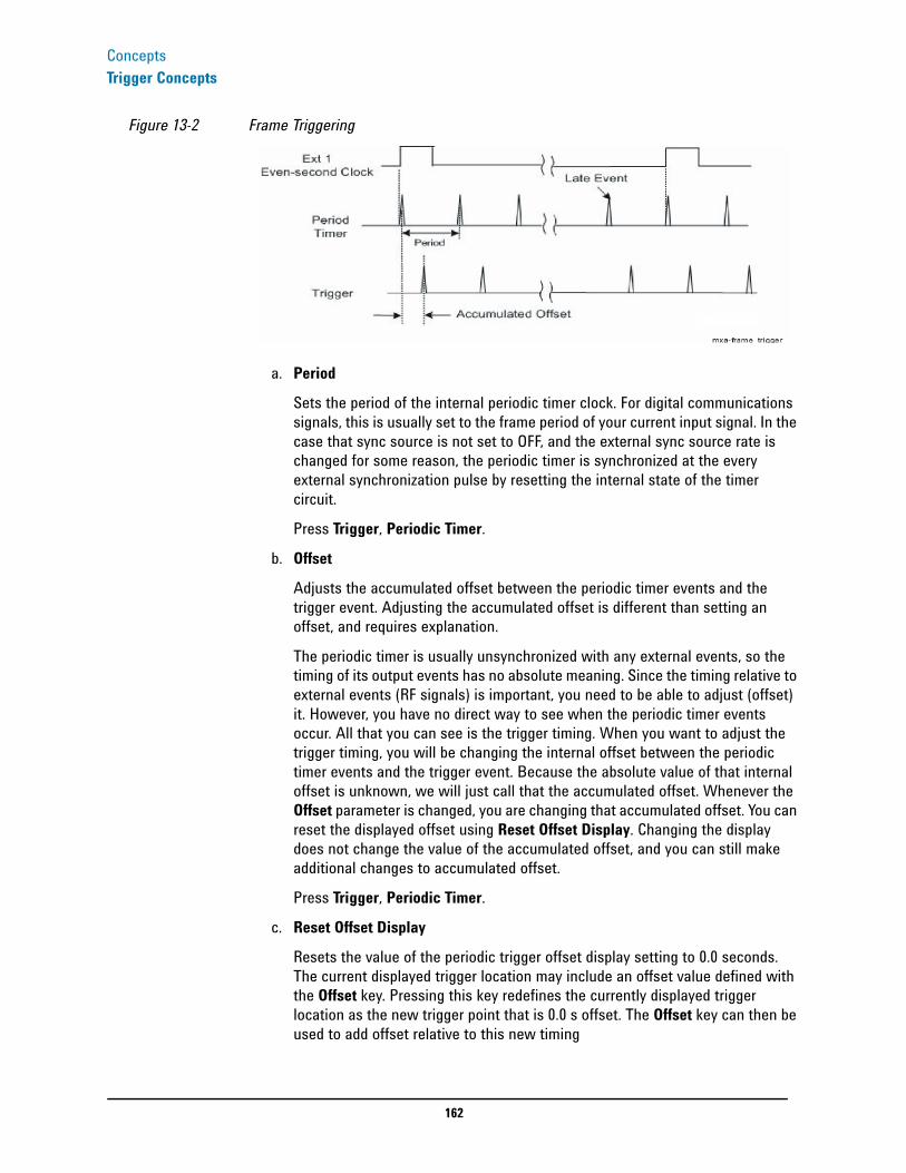
162
ConceptsTrigger Concepts
Figure 13-2 Frame Triggering
a. Period
Sets the period of the internal periodic timer clock. For digital communications signals, this is usually set to the frame period of your current input signal. In the case that sync source is not set to OFF, and the external sync source rate is changed for some reason, the periodic timer is synchronized at the every external synchronization pulse by resetting the internal state of the timer circuit.
Press Trigger, Periodic Timer.
b. Offset
Adjusts the accumulated offset between the periodic timer events and the trigger event. Adjusting the accumulated offset is different than setting an offset, and requires explanation.
The periodic timer is usually unsynchronized with any external events, so the timing of its output events has no absolute meaning. Since the timing relative to external events (RF signals) is important, you need to be able to adjust (offset) it. However, you have no direct way to see when the periodic timer events occur. All that you can see is the trigger timing. When you want to adjust the trigger timing, you will be changing the internal offset between the periodic timer events and the trigger event. Because the absolute value of that internal offset is unknown, we will just call that the accumulated offset. Whenever the Offset parameter is changed, you are changing that accumulated offset. You can reset the displayed offset using Reset Offset Display. Changing the display does not change the value of the accumulated offset, and you can still make additional changes to accumulated offset.
Press Trigger, Periodic Timer.
c. Reset Offset Display
Resets the value of the periodic trigger offset display setting to 0.0 seconds. The current displayed trigger location may include an offset value defined with the Offset key. Pressing this key redefines the currently displayed trigger location as the new trigger point that is 0.0 s offset. The Offset key can then be used to add offset relative to this new timing

163
ConceptsTrigger Concepts
Press Trigger, Periodic Timer.
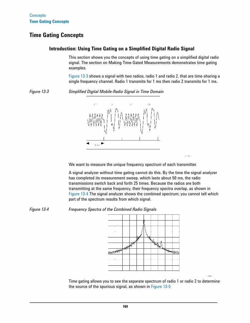
164
ConceptsTime Gating Concepts
Time Gating Concepts
Introduction: Using Time Gating on a Simplified Digital Radio SignalThis section shows you the concepts of using time gating on a simplified digital radio signal. The section on Making Time-Gated Measurements demonstrates time gating examples.
Figure 13-3 shows a signal with two radios, radio 1 and radio 2, that are time-sharing a single frequency channel. Radio 1 transmits for 1 ms then radio 2 transmits for 1 ms.
Figure 13-3 Simplified Digital Mobile-Radio Signal in Time Domain
We want to measure the unique frequency spectrum of each transmitter.
A signal analyzer without time gating cannot do this. By the time the signal analyzer has completed its measurement sweep, which lasts about 50 ms, the radio transmissions switch back and forth 25 times. Because the radios are both transmitting at the same frequency, their frequency spectra overlap, as shown in Figure 13-4 The signal analyzer shows the combined spectrum; you cannot tell which part of the spectrum results from which signal.
Figure 13-4 Frequency Spectra of the Combined Radio Signals
Time gating allows you to see the separate spectrum of radio 1 or radio 2 to determine the source of the spurious signal, as shown in Figure 13-5
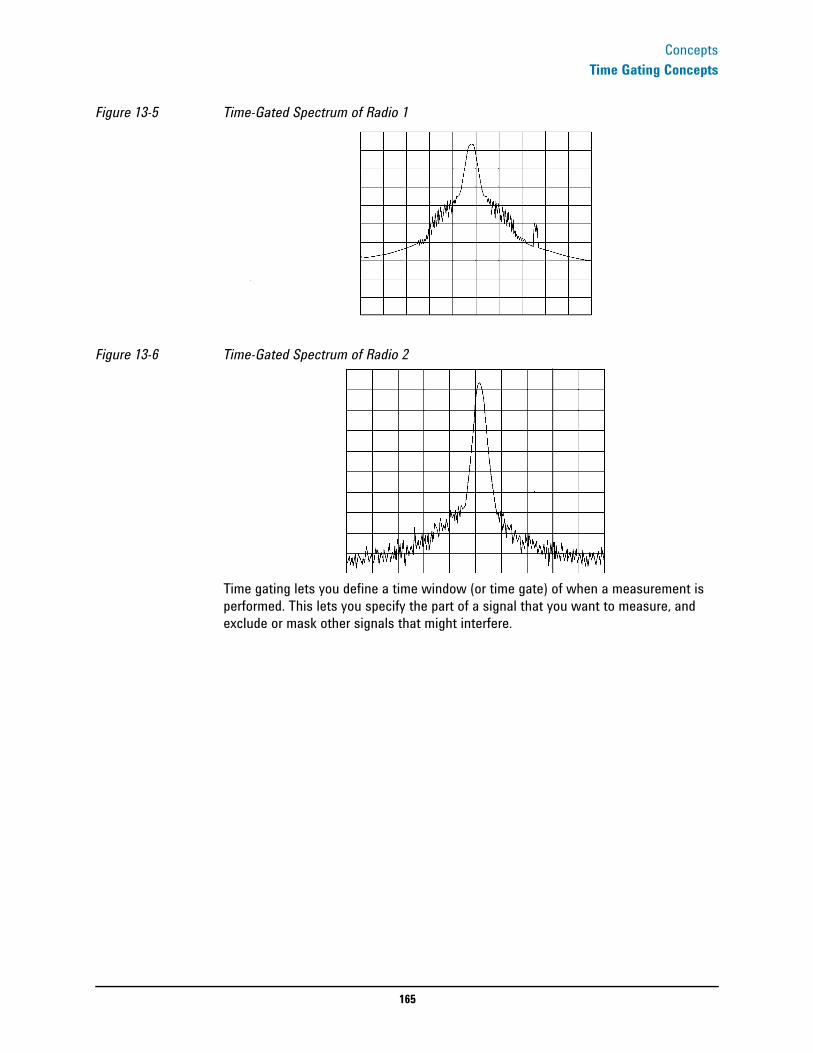
165
ConceptsTime Gating Concepts
Figure 13-5 Time-Gated Spectrum of Radio 1
Figure 13-6 Time-Gated Spectrum of Radio 2
Time gating lets you define a time window (or time gate) of when a measurement is performed. This lets you specify the part of a signal that you want to measure, and exclude or mask other signals that might interfere.
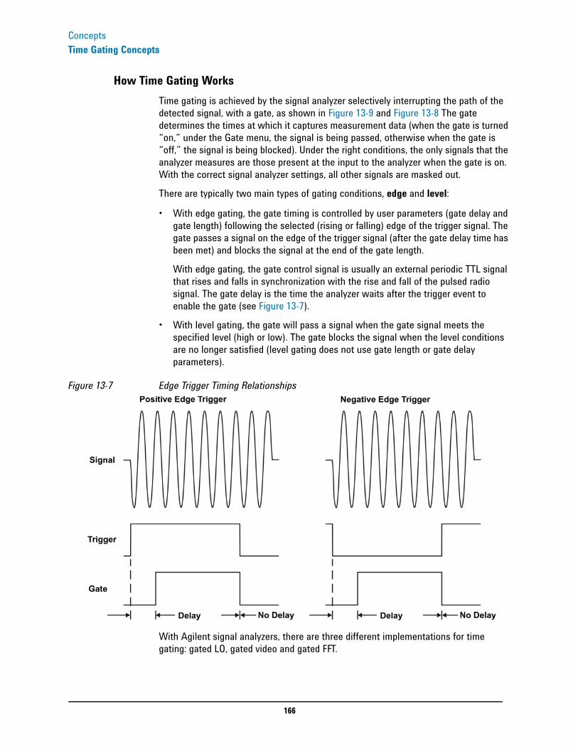
166
ConceptsTime Gating Concepts
How Time Gating Works Time gating is achieved by the signal analyzer selectively interrupting the path of the detected signal, with a gate, as shown in Figure 13-9 and Figure 13-8 The gate determines the times at which it captures measurement data (when the gate is turned “on,” under the Gate menu, the signal is being passed, otherwise when the gate is “off,” the signal is being blocked). Under the right conditions, the only signals that the analyzer measures are those present at the input to the analyzer when the gate is on. With the correct signal analyzer settings, all other signals are masked out.
There are typically two main types of gating conditions, edge and level:
• With edge gating, the gate timing is controlled by user parameters (gate delay and gate length) following the selected (rising or falling) edge of the trigger signal. The gate passes a signal on the edge of the trigger signal (after the gate delay time has been met) and blocks the signal at the end of the gate length.
With edge gating, the gate control signal is usually an external periodic TTL signal that rises and falls in synchronization with the rise and fall of the pulsed radio signal. The gate delay is the time the analyzer waits after the trigger event to enable the gate (see Figure 13-7).
• With level gating, the gate will pass a signal when the gate signal meets the specified level (high or low). The gate blocks the signal when the level conditions are no longer satisfied (level gating does not use gate length or gate delay parameters).
Figure 13-7 Edge Trigger Timing Relationships
With Agilent signal analyzers, there are three different implementations for time gating: gated LO, gated video and gated FFT.
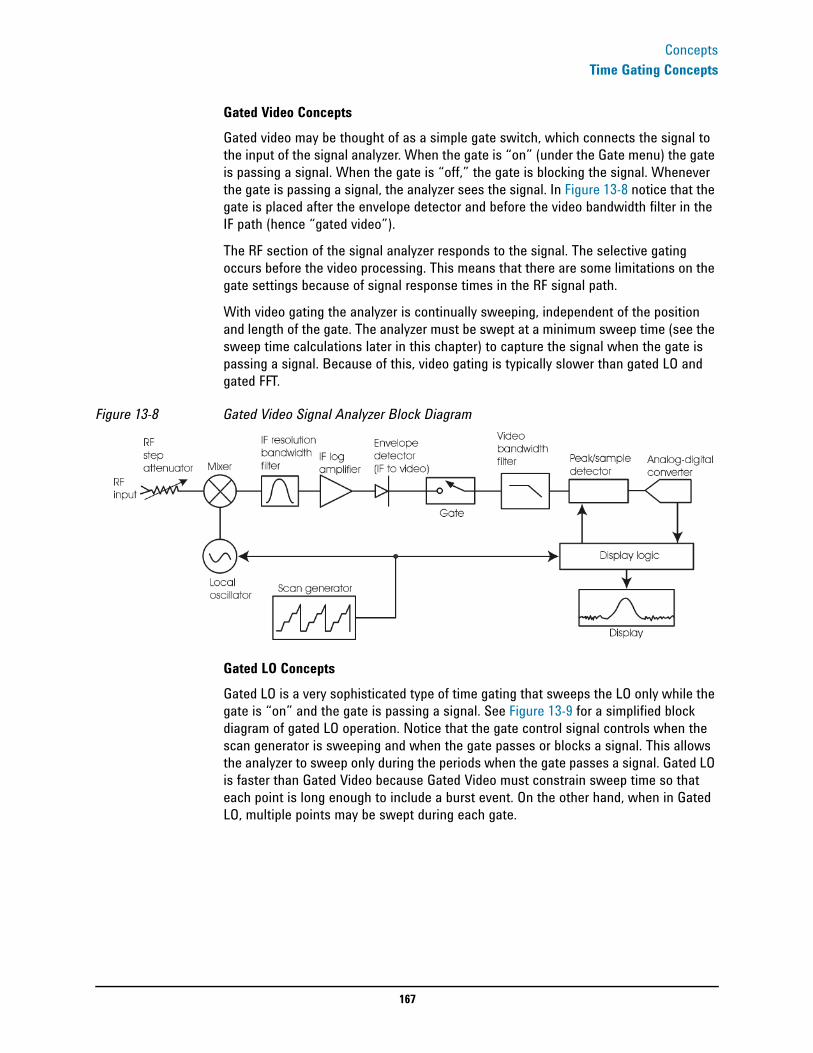
167
ConceptsTime Gating Concepts
Gated Video Concepts Gated video may be thought of as a simple gate switch, which connects the signal to the input of the signal analyzer. When the gate is “on” (under the Gate menu) the gate is passing a signal. When the gate is “off,” the gate is blocking the signal. Whenever the gate is passing a signal, the analyzer sees the signal. In Figure 13-8 notice that the gate is placed after the envelope detector and before the video bandwidth filter in the IF path (hence “gated video”).
The RF section of the signal analyzer responds to the signal. The selective gating occurs before the video processing. This means that there are some limitations on the gate settings because of signal response times in the RF signal path.
With video gating the analyzer is continually sweeping, independent of the position and length of the gate. The analyzer must be swept at a minimum sweep time (see the sweep time calculations later in this chapter) to capture the signal when the gate is passing a signal. Because of this, video gating is typically slower than gated LO and gated FFT.
Figure 13-8 Gated Video Signal Analyzer Block Diagram
Gated LO Concepts Gated LO is a very sophisticated type of time gating that sweeps the LO only while the gate is “on” and the gate is passing a signal. See Figure 13-9 for a simplified block diagram of gated LO operation. Notice that the gate control signal controls when the scan generator is sweeping and when the gate passes or blocks a signal. This allows the analyzer to sweep only during the periods when the gate passes a signal. Gated LO is faster than Gated Video because Gated Video must constrain sweep time so that each point is long enough to include a burst event. On the other hand, when in Gated LO, multiple points may be swept during each gate.
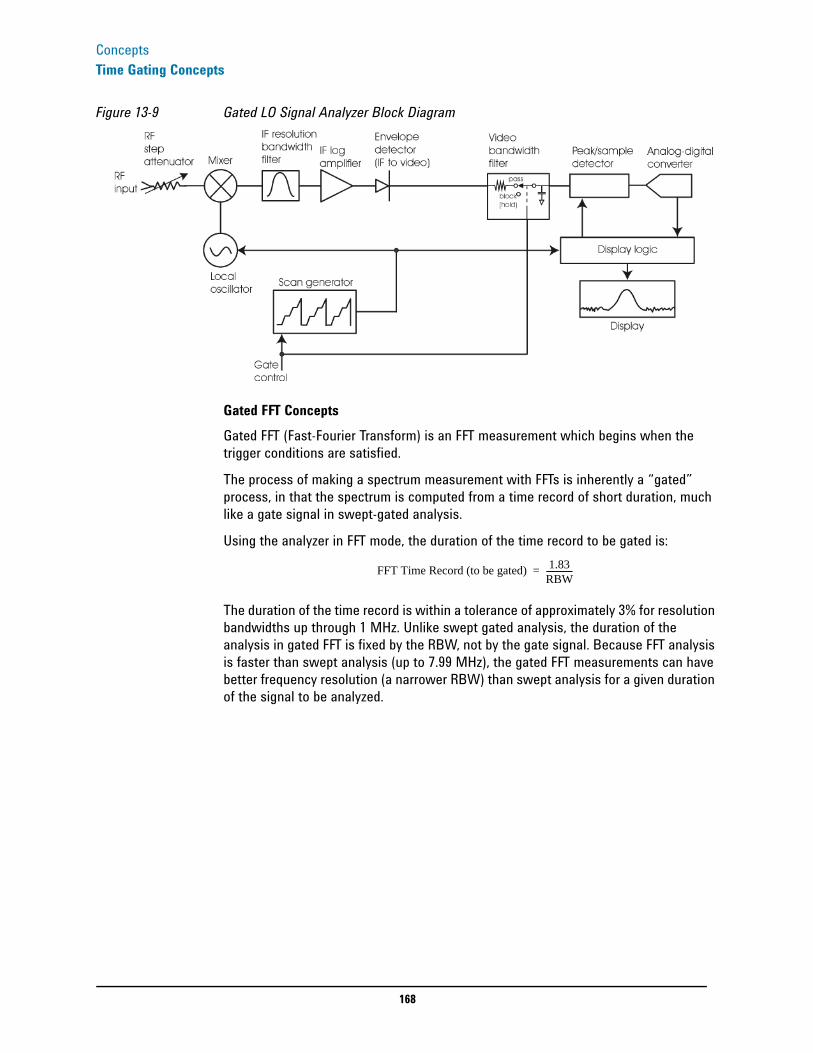
168
ConceptsTime Gating Concepts
Figure 13-9 Gated LO Signal Analyzer Block Diagram
Gated FFT Concepts Gated FFT (Fast-Fourier Transform) is an FFT measurement which begins when the trigger conditions are satisfied.
The process of making a spectrum measurement with FFTs is inherently a “gated” process, in that the spectrum is computed from a time record of short duration, much like a gate signal in swept-gated analysis.
Using the analyzer in FFT mode, the duration of the time record to be gated is:
The duration of the time record is within a tolerance of approximately 3% for resolution bandwidths up through 1 MHz. Unlike swept gated analysis, the duration of the analysis in gated FFT is fixed by the RBW, not by the gate signal. Because FFT analysis is faster than swept analysis (up to 7.99 MHz), the gated FFT measurements can have better frequency resolution (a narrower RBW) than swept analysis for a given duration of the signal to be analyzed.
FFT Time Record (to be gated) 1.83RBW-------------=
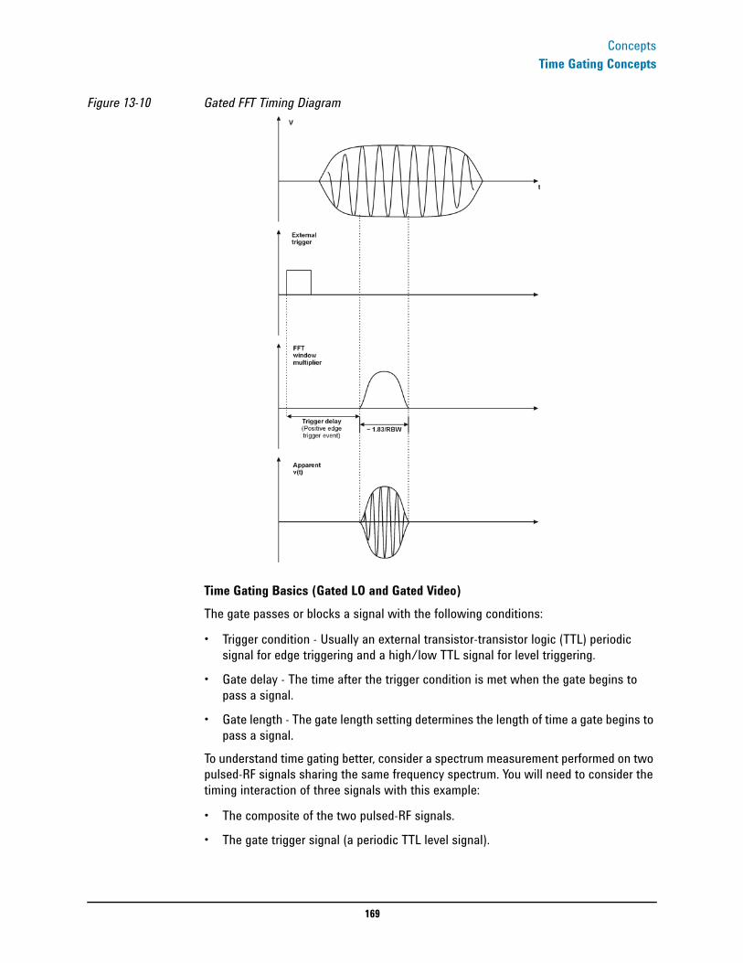
169
ConceptsTime Gating Concepts
Figure 13-10 Gated FFT Timing Diagram
Time Gating Basics (Gated LO and Gated Video)The gate passes or blocks a signal with the following conditions:
• Trigger condition - Usually an external transistor-transistor logic (TTL) periodic signal for edge triggering and a high/low TTL signal for level triggering.
• Gate delay - The time after the trigger condition is met when the gate begins to pass a signal.
• Gate length - The gate length setting determines the length of time a gate begins to pass a signal.
To understand time gating better, consider a spectrum measurement performed on two pulsed-RF signals sharing the same frequency spectrum. You will need to consider the timing interaction of three signals with this example:
• The composite of the two pulsed-RF signals.
• The gate trigger signal (a periodic TTL level signal).
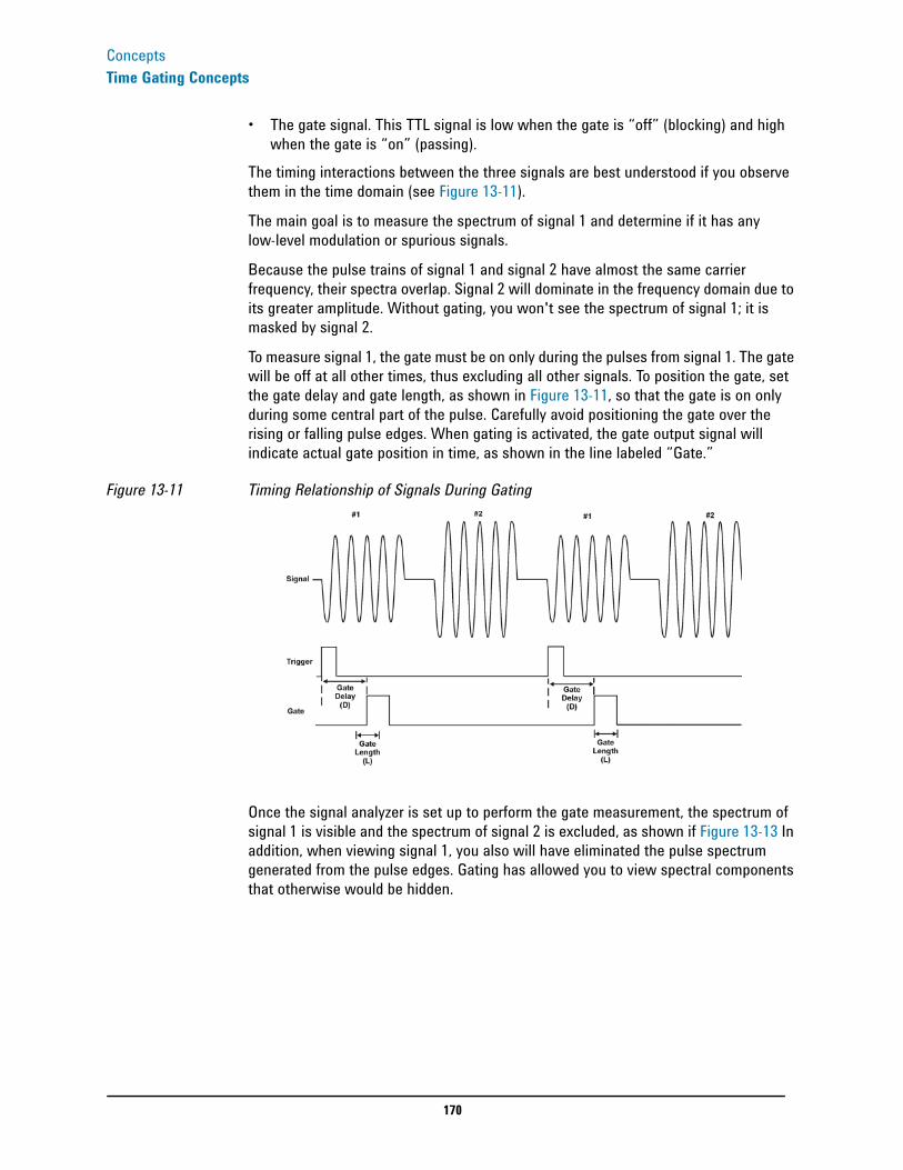
170
ConceptsTime Gating Concepts
• The gate signal. This TTL signal is low when the gate is “off” (blocking) and high when the gate is “on” (passing).
The timing interactions between the three signals are best understood if you observe them in the time domain (see Figure 13-11).
The main goal is to measure the spectrum of signal 1 and determine if it has any low-level modulation or spurious signals.
Because the pulse trains of signal 1 and signal 2 have almost the same carrier frequency, their spectra overlap. Signal 2 will dominate in the frequency domain due to its greater amplitude. Without gating, you won't see the spectrum of signal 1; it is masked by signal 2.
To measure signal 1, the gate must be on only during the pulses from signal 1. The gate will be off at all other times, thus excluding all other signals. To position the gate, set the gate delay and gate length, as shown in Figure 13-11, so that the gate is on only during some central part of the pulse. Carefully avoid positioning the gate over the rising or falling pulse edges. When gating is activated, the gate output signal will indicate actual gate position in time, as shown in the line labeled “Gate.”
Figure 13-11 Timing Relationship of Signals During Gating
Once the signal analyzer is set up to perform the gate measurement, the spectrum of signal 1 is visible and the spectrum of signal 2 is excluded, as shown if Figure 13-13 In addition, when viewing signal 1, you also will have eliminated the pulse spectrum generated from the pulse edges. Gating has allowed you to view spectral components that otherwise would be hidden.
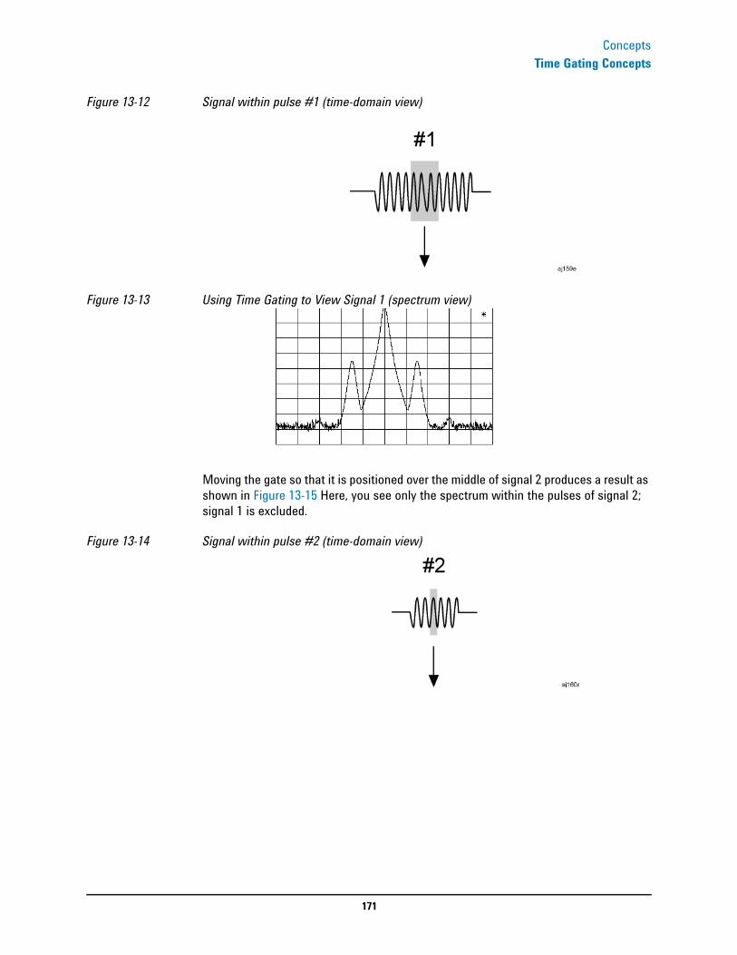
171
ConceptsTime Gating Concepts
Figure 13-12 Signal within pulse #1 (time-domain view)
Figure 13-13 Using Time Gating to View Signal 1 (spectrum view)
Moving the gate so that it is positioned over the middle of signal 2 produces a result as shown in Figure 13-15 Here, you see only the spectrum within the pulses of signal 2; signal 1 is excluded.
Figure 13-14 Signal within pulse #2 (time-domain view)

172
ConceptsTime Gating Concepts
Figure 13-15 Using Time Gating to View Signal 2 (spectrum view)
Measuring a Complex/Unknown Signal
NOTE The steps below help to determine the signal analyzer settings when using time gating. The steps apply to the time gating approaches using gated LO and gated video.
This example shows you how to use time gating to measure a very specific signal. Most signals requiring time gating are fairly complex and in some cases extra steps may be required to perform a measurement.
Step 1. Determine how your signal under test appears in the time domain and how it is synchronized to the trigger signal.
You need to do this to position the time gate by setting the delay relative to the trigger signal. To set the delay, you need to know the timing relationship between the trigger and the signal under test. Unless you already have a good idea of how the two signals look in the time domain, you can examine the signals with an oscilloscope to determine the following parameters:
• Trigger type (edge or level triggering)
• Pulse repetition interval (PRI), which is the length of time between trigger events (the trigger period).
• Pulse width, or τ
• Signal delay (SD), which is the length of time occurring between the trigger event and when the signal is present and stable. If your trigger occurs at the same time as the signal, signal delay will be zero.
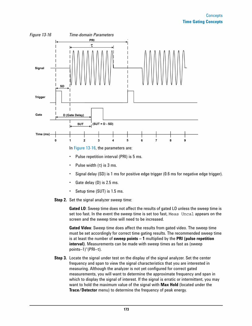
173
ConceptsTime Gating Concepts
Figure 13-16 Time-domain Parameters
In Figure 13-16, the parameters are:
• Pulse repetition interval (PRI) is 5 ms.
• Pulse width (τ) is 3 ms.
• Signal delay (SD) is 1 ms for positive edge trigger (0.6 ms for negative edge trigger).
• Gate delay (D) is 2.5 ms.
• Setup time (SUT) is 1.5 ms.
Step 2. Set the signal analyzer sweep time:
Gated LO: Sweep time does not affect the results of gated LO unless the sweep time is set too fast. In the event the sweep time is set too fast, Meas Uncal appears on the screen and the sweep time will need to be increased.
Gated Video: Sweep time does affect the results from gated video. The sweep time must be set accordingly for correct time gating results. The recommended sweep time is at least the number of sweep points – 1 multiplied by the PRI (pulse repetition interval). Measurements can be made with sweep times as fast as (sweep points–1)*(PRI–τ).
Step 3. Locate the signal under test on the display of the signal analyzer. Set the center frequency and span to view the signal characteristics that you are interested in measuring. Although the analyzer is not yet configured for correct gated measurements, you will want to determine the approximate frequency and span in which to display the signal of interest. If the signal is erratic or intermittent, you may want to hold the maximum value of the signal with Max Hold (located under the Trace/Detector menu) to determine the frequency of peak energy.

174
ConceptsTime Gating Concepts
To optimize measurement speed in the Gated LO case, set the span narrow enough so that the display will still show the signal characteristics you want to measure. For example, if you wanted to look for spurious signals within a 200 kHz frequency range, you might set the frequency span to just over 200 kHz.
Step 4. Determine the setup time and signal delay to set up the gate signal. Turn on the gate and adjust the gate parameters including gate delay and gate length as shown below.
Generally, the gate should be positioned over a part of the signal that is stable, not over a pulse edge or other transition that might disturb the spectrum. Starting the gate at the center of the pulse gives a setup time of about half the pulse width. Setup time describes the length of time during which that signal is present and stable before the gate comes on. The setup time (SUT) must be long enough for the RBW filters to settle following the burst-on transients. Signal delay (SD) is the length of time after the trigger, but before the signal of interest occurs and becomes stable. If the trigger occurs simultaneously with the signal of interest, SD is equal to zero, and SUT is equal to the gate delay. Otherwise, SUT is equal to the gate delay minus SD. See Figure 13-17
Figure 13-17 Positioning the Gate
There is flexibility in positioning the gate, but some positions offer a wider choice of resolution bandwidths. A good rule of thumb is to position the gate from 20 % to 90 % of the burst width. Doing so provides a reasonable compromise between setup time and gate length.
Figure 13-18 Best Position for Gate
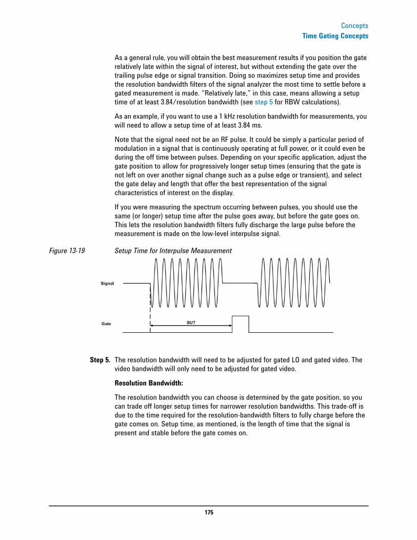
175
ConceptsTime Gating Concepts
As a general rule, you will obtain the best measurement results if you position the gate relatively late within the signal of interest, but without extending the gate over the trailing pulse edge or signal transition. Doing so maximizes setup time and provides the resolution bandwidth filters of the signal analyzer the most time to settle before a gated measurement is made. “Relatively late,” in this case, means allowing a setup time of at least 3.84/resolution bandwidth (see step 5 for RBW calculations).
As an example, if you want to use a 1 kHz resolution bandwidth for measurements, you will need to allow a setup time of at least 3.84 ms.
Note that the signal need not be an RF pulse. It could be simply a particular period of modulation in a signal that is continuously operating at full power, or it could even be during the off time between pulses. Depending on your specific application, adjust the gate position to allow for progressively longer setup times (ensuring that the gate is not left on over another signal change such as a pulse edge or transient), and select the gate delay and length that offer the best representation of the signal characteristics of interest on the display.
If you were measuring the spectrum occurring between pulses, you should use the same (or longer) setup time after the pulse goes away, but before the gate goes on. This lets the resolution bandwidth filters fully discharge the large pulse before the measurement is made on the low-level interpulse signal.
Figure 13-19 Setup Time for Interpulse Measurement
Step 5. The resolution bandwidth will need to be adjusted for gated LO and gated video. The video bandwidth will only need to be adjusted for gated video.
Resolution Bandwidth:
The resolution bandwidth you can choose is determined by the gate position, so you can trade off longer setup times for narrower resolution bandwidths. This trade-off is due to the time required for the resolution-bandwidth filters to fully charge before the gate comes on. Setup time, as mentioned, is the length of time that the signal is present and stable before the gate comes on.
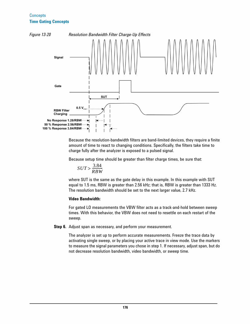
176
ConceptsTime Gating Concepts
Figure 13-20 Resolution Bandwidth Filter Charge-Up Effects
Because the resolution-bandwidth filters are band-limited devices, they require a finite amount of time to react to changing conditions. Specifically, the filters take time to charge fully after the analyzer is exposed to a pulsed signal.
Because setup time should be greater than filter charge times, be sure that:
where SUT is the same as the gate delay in this example. In this example with SUT equal to 1.5 ms, RBW is greater than 2.56 kHz; that is, RBW is greater than 1333 Hz. The resolution bandwidth should be set to the next larger value, 2.7 kHz.
Video Bandwidth:
For gated LO measurements the VBW filter acts as a track-and-hold between sweep times. With this behavior, the VBW does not need to resettle on each restart of the sweep.
Step 6. Adjust span as necessary, and perform your measurement.
The analyzer is set up to perform accurate measurements. Freeze the trace data by activating single sweep, or by placing your active trace in view mode. Use the markers to measure the signal parameters you chose in step 1. If necessary, adjust span, but do not decrease resolution bandwidth, video bandwidth, or sweep time.
SUT 3.84RBW------------->
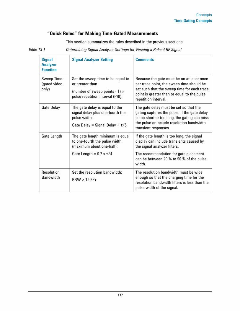
177
ConceptsTime Gating Concepts
“Quick Rules” for Making Time-Gated Measurements This section summarizes the rules described in the previous sections.
Table 13-1 Determining Signal Analyzer Settings for Viewing a Pulsed RF Signal
Signal Analyzer Function
Signal Analyzer Setting Comments
Sweep Time (gated video only)
Set the sweep time to be equal to or greater than(number of sweep points - 1) × pulse repetition interval (PRI):
Because the gate must be on at least once per trace point, the sweep time should be set such that the sweep time for each trace point is greater than or equal to the pulse repetition interval.
Gate Delay The gate delay is equal to the signal delay plus one-fourth the pulse width:Gate Delay = Signal Delay + τ/5
The gate delay must be set so that the gating captures the pulse. If the gate delay is too short or too long, the gating can miss the pulse or include resolution bandwidth transient responses.
Gate Length The gate length minimum is equal to one-fourth the pulse width (maximum about one-half):Gate Length = 0.7 x τ/4
If the gate length is too long, the signal display can include transients caused by the signal analyzer filters.The recommendation for gate placement can be between 20 % to 90 % of the pulse width.
Resolution Bandwidth
Set the resolution bandwidth:RBW > 19.5/τ
The resolution bandwidth must be wide enough so that the charging time for the resolution bandwidth filters is less than the pulse width of the signal.

178
ConceptsTime Gating Concepts
Figure 13-21 Gate Positioning Parameters
Most control settings are determined by two key parameters of the signal under test: the pulse repetition interval (PRI) and the pulse width (τ). If you know these parameters, you can begin by picking some standard settings. Table 13-2 summarizes the parameters for a signal whose trigger event occurs at the same time as the beginning of the pulse (in other words, SD is 0). If your signal has a non-zero delay, just add it to the recommended gate delay.
Table 13-2 Suggested Initial Settings for Known Pulse Width (τ) and Zero Signal Delay
Pulse width (τ) Gate Delay (SD + τ/5)
Resolution Bandwidth (>19.5/τ)
Gate Length (0.7 x τ/4)
4 μs 0.8 μs 4.875 MHz 0.7 μs
10 μs 2 μs 1.95 MHz 1.753 μs
50 μs 10 μs 390 kHz 8.75 μs
63.5 μs 12.7 μs 307 kHz 11.11 μs
100 μs 20 μs 195 kHz 17.5 μs
500 μs 100 μs 39 kHz 87.5 μs
1 ms 200 μs 19.5 kHz 0.175 μs
5 ms 1 ms 3.9 kHz 0.875 ms
10 ms 2 ms 1.95 kHz 1.75 ms
16.6 ms 3.32 ms 1.175 kHz 2.905 ms
33 ms 6.6 ms 591 Hz 5.775 ms
50 ms 10 ms 390 Hz 8.75 ms

179
ConceptsTime Gating Concepts
100 ms 20 ms 195 Hz 17.5 ms
≥130 ms 26 ms 151 Hz 22.75 ms
Table 13-3 If You Have a Problem with the Time-Gated Measurement
Symptom Possible Causes Suggested Solution
Erratic analyzer trace with dropouts that are not removed by increasing analyzer sweep time; oscilloscope view of gate output signal jumps erratically in time domain.
Gate Delay may be greater than trigger repetition interval.
Reduce Gate Delay until it is less than trigger interval.Check Gate View to make sure the gate delay is timed properly.
Gate does not trigger. 1) Gate trigger voltage may be wrong. 2) Gate may not be activated. 3) Gate Source selection may be wrong.
With external gate trigger: ensure that the trigger threshold is set near the midpoint of the waveform (view the waveform on and oscilloscope using high input impedance, not 50 Ω). With RF Burst Gate Source: ensure that the start and stop frequencies are within 10 MHz of the center frequency of the carrier. Check to see if other connections to trigger signal may be reducing voltage. If using an oscilloscope, check that all inputs are high impedance, not 50 Ω.
Display spectrum does not change when the gate is turned on.
Insufficient setup time. Increase setup time for the current resolution bandwidth, or increase resolution bandwidth.
Displayed spectrum too low in amplitude.
Resolution bandwidth or video bandwidth filters not charging fully.
Widen resolution bandwidth or video bandwidth, or both.
Table 13-2 Suggested Initial Settings for Known Pulse Width (τ) and Zero Signal Delay
Pulse width (τ) Gate Delay (SD + τ/5)
Resolution Bandwidth (>19.5/τ)
Gate Length (0.7 x τ/4)
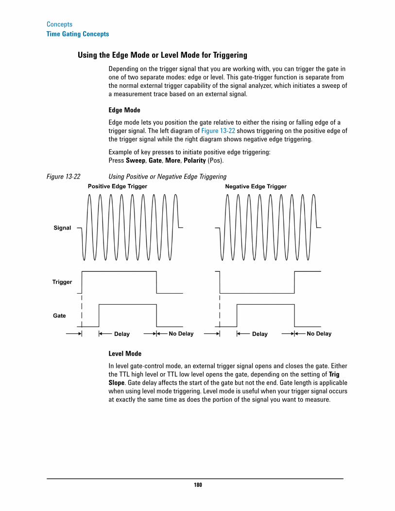
180
ConceptsTime Gating Concepts
Using the Edge Mode or Level Mode for Triggering Depending on the trigger signal that you are working with, you can trigger the gate in one of two separate modes: edge or level. This gate-trigger function is separate from the normal external trigger capability of the signal analyzer, which initiates a sweep of a measurement trace based on an external signal.
Edge Mode Edge mode lets you position the gate relative to either the rising or falling edge of a trigger signal. The left diagram of Figure 13-22 shows triggering on the positive edge of the trigger signal while the right diagram shows negative edge triggering.
Example of key presses to initiate positive edge triggering: Press Sweep, Gate, More, Polarity (Pos).
Figure 13-22 Using Positive or Negative Edge Triggering
Level ModeIn level gate-control mode, an external trigger signal opens and closes the gate. Either the TTL high level or TTL low level opens the gate, depending on the setting of Trig Slope. Gate delay affects the start of the gate but not the end. Gate length is applicable when using level mode triggering. Level mode is useful when your trigger signal occurs at exactly the same time as does the portion of the signal you want to measure.

181
ConceptsTime Gating Concepts
Noise Measurements Using Time GatingTime gating can be used to measure many types of signals. Noise and noise-like signals are often a special case in spectrum analysis. With the history of gated measurements, these signals are especially noteworthy.
The average detector is the best detector to use for measuring noise-like signals because it uses all the available noise power all the time in its measurement. The sample detector is also a good choice because it, too, is free from the peak biases of the peak detector, normal and negative peak detectors.
When using the average or sample detector, noise density measurements using the noise marker or band/interval density marker can be made without any consideration of the use of gating--gated measurements work just as well as non-gated measurements. Thus, the average detector is recommended for noise density measurements.
Older analyzers only had the gated video version of gating available, and these only worked with the peak detector, so the rest of this section will discuss the trade-offs associated with trying to replicate these measurements with an X-Series analyzer.
Unlike older analyzers, X-Series analyzers can make competent measurements of noise density using the noise marker with all detectors, not just those that are ideal for noise measurements. Thus, X-Series analyzers can make noise density measurements with peak detection, compensating for the extent to which peak detection increases the average response of the analyzer to noise. When comparing a gated video measurement using the noise marker between an X-Series and an older analyzer where both use the peak detector, the X-Series answer will be approximately correct, while the older analyzer will need a correction factor. That correction factor is discussed in Agilent Technologies Application Note 1303, Spectrum Analyzer Measurements and Noise, in the section on Peak-detected Noise and TDMA ACP Measurements.
When making measurements of Band/Interval Power or Band/Interval Density, the analyzer does not make compensations for peak detection. For best measurements with these marker functions, average or sample detection should be used.
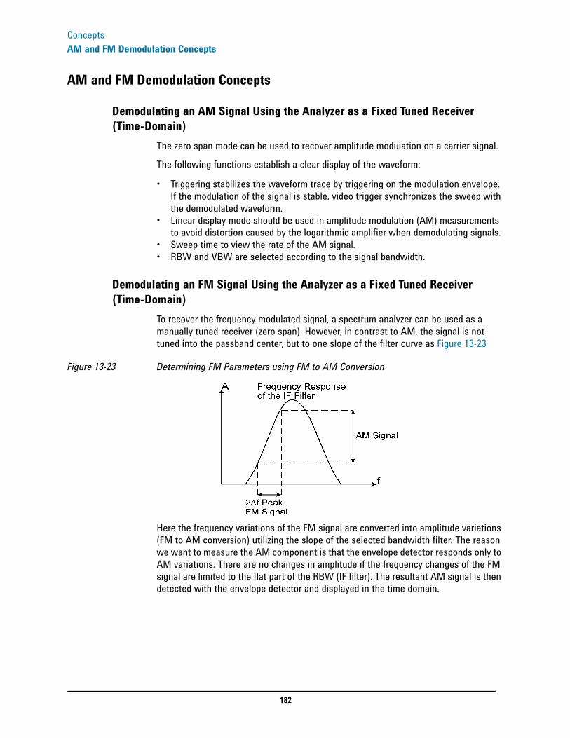
182
ConceptsAM and FM Demodulation Concepts
AM and FM Demodulation Concepts
Demodulating an AM Signal Using the Analyzer as a Fixed Tuned Receiver (Time-Domain)
The zero span mode can be used to recover amplitude modulation on a carrier signal.
The following functions establish a clear display of the waveform:
• Triggering stabilizes the waveform trace by triggering on the modulation envelope. If the modulation of the signal is stable, video trigger synchronizes the sweep with the demodulated waveform.
• Linear display mode should be used in amplitude modulation (AM) measurements to avoid distortion caused by the logarithmic amplifier when demodulating signals.
• Sweep time to view the rate of the AM signal.• RBW and VBW are selected according to the signal bandwidth.
Demodulating an FM Signal Using the Analyzer as a Fixed Tuned Receiver (Time-Domain)
To recover the frequency modulated signal, a spectrum analyzer can be used as a manually tuned receiver (zero span). However, in contrast to AM, the signal is not tuned into the passband center, but to one slope of the filter curve as Figure 13-23
Figure 13-23 Determining FM Parameters using FM to AM Conversion
Here the frequency variations of the FM signal are converted into amplitude variations (FM to AM conversion) utilizing the slope of the selected bandwidth filter. The reason we want to measure the AM component is that the envelope detector responds only to AM variations. There are no changes in amplitude if the frequency changes of the FM signal are limited to the flat part of the RBW (IF filter). The resultant AM signal is then detected with the envelope detector and displayed in the time domain.

183
ConceptsIQ Analysis Concepts
IQ Analysis Concepts
Purpose IQ Analysis (Basic) mode is used to capture complex time domain data from wide bandwidth RF signals. This mode preserves the instantaneous vector relationships of time, frequency, phase and amplitude contained within the selected digitizer span or analysis BW, at the analyzer's center frequency, for output as IQ data. This IQ data can then be utilized internally or output over LAN, USB or GPIB for use with external analysis tools. Each measurement description specifies the types of data available remotely for that measurement.
Within the IQ Analyzer mode, basic frequency domain, time domain and IQ measurements are available as initial signal and data verification tools in preparation for deriving the IQ data output. This is accomplished using the Complex Spectrum and IQ Waveform measurements. Although Complex Spectrum and IQ Waveform are defined as measurements in the IQ Analyzer (Basic) mode, they act primarily as tools to verify the signals and data as stated above.
Complex Spectrum Measurement
Purpose This measurement is FFT (Fast Fourier Transform) based. The FFT-specific parameters are located in the Advanced menu. The Complex Spectrum measurement provides a display in the upper window of power versus frequency with current (yellow trace) and average (blue trace) data. In addition, an IQ waveform of voltage versus time is provided in the lower window. One advantage of having an I/Q view available while in the spectrum measurement is that it allows you to view complex components of the same signal without changing settings or measurements.
Measurement MethodThe measurement uses digital signal processing to sample the input signal and convert it to the frequency domain. With the instrument tuned to a fixed center frequency, samples are digitized at a high rate, converted to I and Q components with DSP hardware, and then converted to the frequency domain with FFT software.
Troubleshooting HintsChanges made by the user to advanced spectrum settings, particularly to ADC range settings, can inadvertently result in spectrum measurements that are invalid and cause error messages to appear. Care needs to be taken when using advanced features.
IQ Waveform Measurement
Purpose The IQ Waveform measurement provides a time domain view of the RF signal envelope with power versus time or an IQ waveform with the I and Q signal waveforms in parameters of voltage versus time. The RF Envelope view provides the power verses
184
ConceptsIQ Analysis Concepts
time display, and the I/Q Waveform view provides the voltage versus time display. One advantage of having an I/Q Waveform view available while making a waveform measurement is that it allows you to view complex components of the same signal without changing settings or measurements.
The waveform measurement can be used to perform general purpose power measurements in the time domain with excellent accuracy.
Measurement MethodThe instrument makes repeated power measurements at a set frequency, similar to the way a swept-tuned signal analyzer makes zero span measurements. The input analog signal is converted to a digital signal, which then is processed into a representation of a waveform measurement. The measurement relies on a high rate of sampling to create an accurate representation of a time domain signal.
185
ConceptsSpurious Emissions Measurement Concepts
Spurious Emissions Measurement Concepts
Purpose Spurious signals can be caused by different combinations of signals in the transmitter. The spurious emissions from the transmitter should be minimized to guarantee minimum interference with other frequency channels in the system. Harmonics are distortion products caused by nonlinear behavior in the transmitter. They are integer multiples of the transmitted signal carrier frequency.
This measurement verifies the frequency ranges of interest are free of interference by measuring the spurious signals specified by the user defined range table.
Measurement MethodThe table-driven measurement has the flexibility to set up custom parameters such as frequency, span, resolution bandwidth, and video bandwidth. Up to the top 40 spurs can be viewed
For each range that you specify and activate, the analyzer scans the band using the specified Range Table settings. Then using the Peak Excursion and Peak Threshold values determines which spurs to report.
As each band is swept, any signal which is above the Peak Threshold value and has a peak excursion of greater than the Peak Excursion value will be added to a list of spurs displayed in the lower results window. A total of 200 spurs can be recorded for one measurement, with a limit of 10 spurs per frequency range. To improve repeatability, you can increase the number of averages.
From the spurs in the list, those with peak amplitude greater than the Absolute Limit for that range will be logged as a measurement failure and denoted by an 'F' in the 'Amplitude' column of the table. If no spurs are reported, but the measured trace exceeds the limit line for any range, the fail flag is set to fail.
This measurement has the ability to display two traces using different detectors on the display simultaneously. All spur detection and limit line testing are only applied to the trace associated with Detector 1, which will be colored yellow. The trace associated with Detector 2 will be colored cyan.
If the sweep time for the range exceeds 2 seconds, a flashing message “Sweeping...Please Wait” will appear in the annunciator area. This advises you that the time to complete the sweep is between 2 and 2000 seconds, and is used as without it the display would appear stagnant and you may think the measurement is not functional.
186
ConceptsSpectrum Emission Mask Measurement Concepts
Spectrum Emission Mask Measurement Concepts
PurposeThe Spectrum Emission Mask measurement includes the in-band and out-of-band spurious emissions. As it applies to W-CDMA (3GPP), this is the power contained in a specified frequency bandwidth at certain offsets relative to the total carrier power. It may also be expressed as a ratio of power spectral densities between the carrier and the specified offset frequency band.
This spectrum emission mask measurement is a composite measurement of out-of-channel emissions, combining both in-band and out-of-band specifications. It provides useful figures-of-merit for the spectral regrowth and emissions produced by components and circuit blocks, without the rigor of performing a full spectrum emissions mask measurement.
Measurement MethodThe spectrum emission mask measurement measures spurious signal levels in up to five pairs of offset/region frequencies and relates them to the carrier power. The reference channel integration bandwidth method is used to measure the carrier channel power and offset/region powers. When Offset is selected, spectrum emission mask measurements are made, relative to the carrier channel frequency bandwidth. When Region is selected, spurious emission absolute measurements are made, set by specifying start and stop RF frequencies. The upper frequency range limit is 3.678 GHz.
This integration bandwidth method is used to perform a data acquisition. In this process, the reference channel integration bandwidth (Meas BW) is analyzed using the automatically defined resolution bandwidth (Res BW), which is much narrower than the channel bandwidth. The measurement computes an average power of the channel or offset/region over a specified number of data acquisitions, automatically compensating for resolution bandwidth and noise bandwidth.
This measurement requires the user to specify the measurement bandwidths of carrier channel and each of the offset/region frequency pairs up to 5. Each pair may be defined with unique measurement bandwidths. The results are displayed both as relative power in dBc, and as absolute power in dBm.

187
ConceptsOccupied Bandwidth Measurement Concepts
Occupied Bandwidth Measurement Concepts
PurposeOccupied bandwidth measures the bandwidth containing 99.0 of the total transmission power.
The spectrum shape of a signal can give useful qualitative insight into transmitter operation. Any distortion to the spectrum shape can indicate problems in transmitter performance.
Measurement MethodThe instrument uses digital signal processing (DSP) to sample the input signal and convert it to the frequency domain. With the instrument tuned to a fixed center frequency, samples are digitized at a high rate with DSP hardware, and then converted to the frequency domain with FFT software.
The total absolute power within the measurement frequency span is integrated for its 100% of power. The lower and upper frequencies containing 0.5% each of the total power are then calculated to get 99.0% bandwidth.

188
ConceptsBaseband I/Q Inputs (Option BBA) Measurement Concepts
Baseband I/Q Inputs (Option BBA) Measurement ConceptsThe N9020A Option BBA Baseband I/Q Inputs provides the ability to analyze baseband I/Q signal characteristics of mobile and base station transmitters. This option may be used only in conjunction with the following modes:
• IQ Analyzer (Basic)
• 802.16 OFDMA (WiMAX/WiBro)
• cdma2000
• GSM/EDGE
• TD-SCDMA
What are Baseband I/Q Inputs?Option BBA consists of a Baseband Input module, four input connectors, and a calibration output connector. The connectors are at the left side of the front panel. The two ports labeled “I” and “Q” are the “unbalanced” inputs.
An unbalanced or “single-ended” baseband measurement of an I or Q signal is made using a probe connected to the I or Q connector. A simultaneous I/Q unbalanced single-ended measurement may be made using two probes connected to the I and Q input connectors.
If “balanced” signals are available, they may be used to make a more accurate measurement. Balanced signals are signals present in two separate conductors, are symmetrical about ground, and are opposite in polarity, or out of phase by 180 degrees.
Measurements using balanced signals can have a higher signal to noise ratio resulting in improved accuracy. Noise coupled into each conductor equally in a “common mode” to both signals may be separated from the signal. The measure of this separation is “common-mode rejection”.
To make a balanced measurement, the two connectors labeled “I” and “Q” are used in conjunction with the I and Q inputs. The terms “I-bar” and “Q-bar” may be applied to the signals, as well as the inputs themselves. Probes (customer provided) must be used to input balanced baseband I/Q signals. This may be referred to as a balanced measurement.
Balanced baseband measurements are made using the I and connectors for I only signal measurements, while the Q and connectors are used for a Q only signal measurement. Balanced measurements of I/Q require differential probe connections to all four input connectors. For details of probe selection and use, refer to “Selecting Input Probes for Baseband Measurements” on page 190.
What are Baseband I/Q Signals?In transmitters, the term baseband I/Q refers to signals that are the fundamental products of individual I/Q modulators, before the I and Q component signals are combined, and before upconversion to IF or RF frequencies.

189
ConceptsBaseband I/Q Inputs (Option BBA) Measurement Concepts
In receivers, baseband I/Q analysis may be used to test the I and Q products of I/Q demodulators, after an RF signal has been downconverted and demodulated.
Why Make Measurements at Baseband?Baseband I/Q measurements are a valuable means of making qualitative analyses of the following operating characteristics:
• I/Q signal layer access for performing format-specific demodulation measurements (for example, CDMA, GSM, W-CDMA).
• Modulation accuracy – that is,. I/Q plane metrics:
— rho
— error vector magnitude; rms, peak, or 95%
— carrier feed-through
— frequency error
— magnitude and phase errors• Code-domain analysis (including code-specific metrics)
• CCDF of
• Single sideband (SSB) metrics for assessing output quality
• Basic analysis of I and Q signals in isolation including: DC content, rms and peak to peak levels, CCDF of each channel
Comparisons of measurements made at baseband and RF frequencies produced by the same device are especially revealing. Once signal integrity is verified at baseband, impairments can be traced to specific stages of upconversion, amplification, or filtering by RF analysis. In addition, impairments to signal quality that are apparent at RF frequencies may be traceable to baseband using baseband analysis.
I2 Q2+
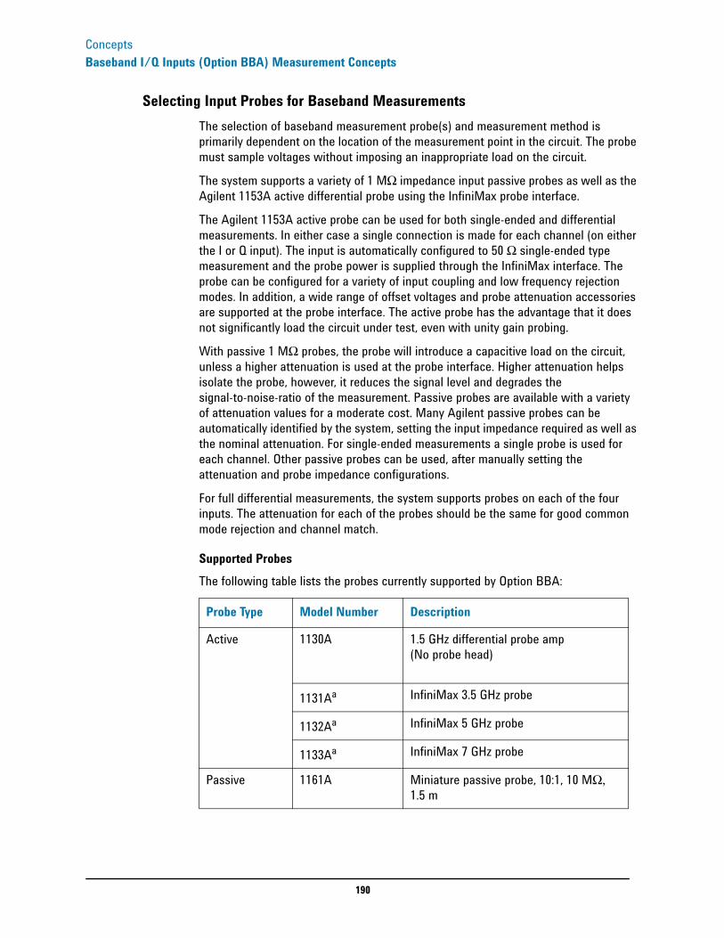
190
ConceptsBaseband I/Q Inputs (Option BBA) Measurement Concepts
Selecting Input Probes for Baseband MeasurementsThe selection of baseband measurement probe(s) and measurement method is primarily dependent on the location of the measurement point in the circuit. The probe must sample voltages without imposing an inappropriate load on the circuit.
The system supports a variety of 1 MΩ impedance input passive probes as well as the Agilent 1153A active differential probe using the InfiniMax probe interface.
The Agilent 1153A active probe can be used for both single-ended and differential measurements. In either case a single connection is made for each channel (on either the I or Q input). The input is automatically configured to 50 Ω single-ended type measurement and the probe power is supplied through the InfiniMax interface. The probe can be configured for a variety of input coupling and low frequency rejection modes. In addition, a wide range of offset voltages and probe attenuation accessories are supported at the probe interface. The active probe has the advantage that it does not significantly load the circuit under test, even with unity gain probing.
With passive 1 MΩ probes, the probe will introduce a capacitive load on the circuit, unless a higher attenuation is used at the probe interface. Higher attenuation helps isolate the probe, however, it reduces the signal level and degrades the signal-to-noise-ratio of the measurement. Passive probes are available with a variety of attenuation values for a moderate cost. Many Agilent passive probes can be automatically identified by the system, setting the input impedance required as well as the nominal attenuation. For single-ended measurements a single probe is used for each channel. Other passive probes can be used, after manually setting the attenuation and probe impedance configurations.
For full differential measurements, the system supports probes on each of the four inputs. The attenuation for each of the probes should be the same for good common mode rejection and channel match.
Supported ProbesThe following table lists the probes currently supported by Option BBA:
Probe Type Model Number Description
Active 1130A
1.5 GHz differential probe amp (No probe head)
1131Aa InfiniMax 3.5 GHz probe
1132Aa InfiniMax 5 GHz probe
1133Aa InfiniMax 7 GHz probe
Passive 1161A Miniature passive probe, 10:1, 10 MΩ, 1.5 m

191
ConceptsBaseband I/Q Inputs (Option BBA) Measurement Concepts
Probes without Stored CalibrationThe following 115xA active probes may be used with the MXA’s baseband IQ inputs and may use the same probe calibration utility software. However, the probe calibration data is not stored in the MXA and will be lost if power is cycled. Use of the E2655B de-skew and calibration kit, including the calibration fixture, is required because of the different physical configuration of the probes. (The physical connections are different mechanically, not electrically.)
Refer to the current Agilent probe data sheet for specific information regarding frequency of operation and power supply requirements.
Baseband I/Q Measurement ViewsMeasurement result views made in the IQ Analyzer (Basic) mode are available for baseband signals if they relate to the nature of the signal itself. Many measurements which relate to the characteristics that baseband I and Q signals have when mixed and upconverted to signals in the RF spectrum can be made as well. However, measurements which relate to the characteristics of an upconverted signal that lie beyond the bandwidth available to the Baseband I/Q Input circuits can not be measured (the limit are dependent on the installed options: Standard – 10 Hz to 20 MHz, Option B25 – 10 Hz to 50 MHz, and Option S40 – 10 Hz to 80 MHz).
At RF frequencies, power measurements are conventionally displayed on a logarithmic vertical scale in dBm units, whereas measurements of baseband signals using Baseband I/Q inputs may be conveniently displayed as voltage using a linear vertical scale as well as a log scale.
Spectrum Views and 0 Hz Center FrequencyTo view the Spectrum display of I only or Q only signals, use the Complex Spectrum measurement capability in IQ Analyzer (Basic) Mode.
I only and Q only Spectrum views are conventional, displayed with 0 Hz at the left side of the horizontal axis. When upconverted or multiplied, an I only or Q only signal could ultimately lie above or below the carrier center frequency, but in either case it will only occupy half the bandwidth.
a. Probe heads are necessary to attach to your device properly. Probe con-nectivity kits such as the E2668A, E2669A or E2675A are needed. For more details, refer to the Agilent probe configuration guide, 5968-7141EN and 5989-6162EN.
Probe Type Model Number Description
Active 1153A 200MHz differential probe
1156A Active probe, 1.5 GHz
1157A Active probe, 2.5 GHz
1158A Active probe, 4 GHz
192
ConceptsBaseband I/Q Inputs (Option BBA) Measurement Concepts
Waveform Signal Envelope Views of I only or Q onlyTo view the Signal Envelope display of I only or Q only signals, use the Waveform measurement capability in IQ Analyzer (Basic) Mode.
The I and Q Waveform of an I/Q signal is very different from the complex signal displayed in the RF Envelope view. That is because the RF Envelope is a product of both the I and Q modulation waveforms.
However, an I and Q Waveform measurement of an I only or Q only signal is exactly the same signal displayed in the RF Envelope view. That is because an I only or Q only waveform determines the I only or Q only signal envelope. Thus, the RF Envelope view can be used to measure an I only or Q only waveform directly.
Index
193
Numerics50 ohm load 1650 ohm/75 ohm minimum loss pad 1675 ohm matching transformer 16
AAC probe 16Accessories 16accessories
50 ohm load 1650 ohm/75 ohm minimum loss pad
1675 ohm matching transformer 16AC probe 16broadband preamplifiers 17GPIB cable 17power splitters 18RF limiters 17transient limiters 17
ACP keyMEAS key 116
ACP measurement 114Adjacent Channel Power measurement
114AM demodulation
time-domain demodulation, manually calculating 182
AM signal demodulation 138amplifiers 17analyzer distortion products 62arrow keys, using 10attenuation
input, reducing 42setting automatically 44setting manually 43
averagingdescription 50types 50
Bband power marker 81Bluetooth power measurement 124broadband preamplifiers 17Burst Power key
Meas key 124Burst Power measurement 124
Ccable
GPIB 17CCDF measurement 119CCDP key
Meas key 120Channel Power key
Meas key 110Channel power measurement 110
channel power measurementnoise-like signals 79
comparing signalstwo signals 20two signals not on the same screen 23
complex spectrum measurement 183Concepts
AM demodulation 182FM demodulation 182
conceptsgated FFT (PSA) 168gated LO (PSA) 167gated video (ESA) 167IF filter, defined 158resolving signals of equal amplitude
158resolving small signals hidden by
large signals 158time gating 164
Ddata, entering from front panel 10DC probes
use of 16delta band marker function 37delta marker 20demodulating
AM 138AM overview 138
detectors, average 48distortion measurements
identifying distortion products 62identifying TOI distortion 65overview 62
distortion products 62drifting signals 59
EEnter key, using 10equipment 15ESD safety accessories 18examples
AM demodulationmanual demodulation 138
average detector, using 48averaging, trace 50distortion
identify distortion products 62TOI 65
frequency accuracy 13frequency drift 56input attenuation, reducing 42marker counter 54measuring
low-level signals 48noise
band power marker 76
channel power, using 79noise marker 72overview 70signal to noise 70
resolution bandwidth, reducing 45signals
low-level, overview 42off-screen, comparing 23on-screen, comparing 20resolving, equal amplitude 26resolving, small signals hidden by
large signals 31signals, viewing 12time gating
ESA-E time gate 102PSA gated FFT 106PSA gated sweep 98
trace averaging 50tracking a signal 59
Ffactory preset, description 11finding hidden signals 158FM demodulation
time-domain demodulation, manually calculating 182
frequency accuracy, increasing 13frequency readout resolution increased
54front panel
entering data 10
Ggate delay
setting the gate delay, time gating 175gate length
setting the gate length, time gating 175
gated FFT (PSA), concepts 168gated LO (PSA), concepts 167gated video (ESA), concepts 167GPIB cable 17
Hharmonic distortion
measuring low-level signals 23
Iidentifying distortion products 62initial setting for time gating 178input attenuation, reducing 42intermodulation distortion, third order
65interval power marker function 37iq waveform measurement 183
194
Index
Kkeypad, using 10knob, using 10
Llimiters
RF and transient 17load, 50 ohm 16low-level signals
harmonics, measuring 23input attenuation, reducing 42resolution bandwidth, reducing 45sweep time, reducing 48trace averaging 50
Mmarker
frequency and amplitude, reading 12moving
to reference level 12with knob or arrow key 12
marker annotationlocation 12
marker counter examplemarker frequency resolution 54
marker functiondelta band 37interval power 37
markersdelta 20
markers, advancedband power 81
markers, advancesnoise marker 81
MEAS keyACP key 116
Meas keyBurst Power key 124CCDP key 120Channel Power key 110Spectrum Emission Mask key 134
measure complex modulation power 37measurement
ACP or spurious emissions mask 185occupied bandwidth 187
spectrum shape 187spectrum emission mask 186
measurementsdistortion 62
identifying 62TOI 65
frequency drift 56, 59noise
band power marker 76channel power 79noise marker 72
overview 70signal to noise 70
time gating 91ESA-E time gate 102PSA gated FFT 106PSA gated sweep 98
moving signals 59
Nnoise marker 81noise measurements
band power marker, using 76channel power, using 79noise marker, using 72overview 70signal to noise 70sweep time, reducing 48
noise power measurement near noise floor 86
numeric keypad, using 10
Ooccupied bandwidth
99.0% bandwidth 187measurement method 187purpose 187total absolute power 187
Occupied Bandwidth measurement 112overviews
distortion 62low-level signal 42noise 70resolving signals 158time gating 164
Ppositioning the gate, time gating 174power amplifiers 17power diff
trace math function 86power splitters 18preamplifiers 17preset
factory 11types 11user, creating 11
probesAC and DC 16
RRBW selections 47reference level, setting 12resolution bandwidth
adjusting 45resolving signals 158
resolving signals
small signals hidden by large signals 158
resolving two signalsequal amplitude 26, 158
resolving, equal amplitude 158RF limiters 17RPG, using 10rules for time gating 177
Ssignal parameters for a time-gated
measurement 172signal tracking
example 59marker tracking 35using to resolve signals 35
signalslow-level, overview 42off-screen, comparing 23on-screen, comparing 20resolving, overview 158separating, overview 158
signals, increasing accuracy 13signals, viewing 12softkeys, auto and man mode 11softkeys, basic types 10Spectrum (Frequency Domain) key
183Spectrum analysis measurement
application 109channel power 79
spectrum emission maskin-band and out-of-band spurious
emissions 186integration bandwidth method 186measurement method 186offset or region frequency pairs 186purpose 186reference channel integration
bandwidth 186spectral regrowth 186
Spectrum Emission Mask keyMeas key 134
Spectrum Emission Mask measurement 133
spectrum measurementmethod 183
splitters 18static safety accessories 18Statistical Power measurement 119sweep time and sensitivity trade off 47sweep time for a time-gated
measurement 102, 173sweep time, changing 48
Ttest equipment 15
Index
195
third order intermodulation distortion example 65
time gatingdescription 164ESA-E time gate, using 102example 91gated FFT (PSA), concepts 168gated LO (PSA), concepts 167gated video (ESA), concepts 167how time gating works 166initial settings 178keys 174positioning the gate 99, 174PSA gated FFT, using 106PSA gated sweep, using 98rules 177setting sweep time 178setting the gate length 175setting the resolution bandwidth 175,
176setting the span 173, 176setting the video bandwidth 175signal parameters 172steps for measuring unknown signals
172sweep time 102, 173triggering
edge mode 180level mode 180negative edge 180positive edge 180
troubleshooting 178time gating measurement 91trace math function
power diff 86tracking unstable signals 59transient limiter 17troubleshooting
time-gated measurements 178
Uunit softkeys, using 10unstable signals 59user preset
creating 11description 11
Wwaveform
method 184Waveform (Time Domain) key 183

196
Index