Embed Size (px)
Citation preview
Ti
Ta
b
c
a
ARRAA
KHSNS
1
wandp
9wiom
0h
Agricultural Water Management 111 (2012) 87– 104
Contents lists available at SciVerse ScienceDirect
Agricultural Water Management
j ourna l ho me page: www.elsev ier .com/ locate /agwat
wo-dimensional modeling of water and nitrogen fate from sweet sorghumrrigated with fresh and blended saline waters
.B. Ramosa,∗, J. Simunekb, M.C. Gonc alvesa,c, J.C. Martinsc, A. Prazeresc, L.S. Pereiraa
CEER-Biosystems Engineering, Institute of Agronomy, Technical University of Lisbon, Tapada da Ajuda, 1349-017, Lisbon, PortugalDepartment of Environmental Sciences, University of California, Riverside, CA, 92521, USAEstac ão Agronómica Nacional, INIA, Instituto Nacional de Recursos Biológicos, Quinta do Marquês, Av. República, 2784-505, Oeiras, Portugal
r t i c l e i n f o
rticle history:eceived 21 October 2011eceived in revised form 18 May 2012ccepted 21 May 2012vailable online 8 June 2012
eywords:YDRUS-2Daline irrigation wateritrates leachingorghum yields
a b s t r a c t
The need for reducing irrigation water demand and non-point source pollution all across Europe has madesweet sorghum [Sorghum bicolor (L.) Moench], due to its lower water and nutrient requirements, an inter-esting alternative to other traditional summer crops in European Mediterranean regions. HYDRUS-2D wasused to model the fate of nitrogen in a plot planted with sweet sorghum grown under Mediterraneanconditions between 2007 and 2010, while considering drip irrigation scenarios with different levels ofnitrogen and salty waters. HYDRUS-2D simulated water contents, ECsw, and N NH4
+ and N NO3− con-
centrations continuously for the entire duration of the field experiment, while producing RMSE betweensimulated and measured data of 0.030 cm3 cm−3, 1.764 dS m−1, 0.042 mmolc L−1, and 3.078 mmolc L−1,respectively. Estimates for sweet sorghum water requirements varied between 360 and 457 mm depend-ing upon the crop season and the irrigation treatment. Sweet sorghum proved to be tolerant to salinewaters if applied only during one crop season. However, the continuous use of saline waters for morethan one crop season led to soil salinization, and to root water uptake reductions due to the increasingsalinity stress. The relation found between N NO3
− uptake and dry biomass yield (R2 = 0.71) showedthat nitrogen needs were smaller than the uptakes estimated for the scenario with the highest levels of
nitrogen application. The movement of N out of the root zone was dependent on the amount of waterflowing through the root zone, the amount of N applied, the form of N in the fertilizer, and the tim-ing and number of fertigation events. The simulations with HYDRUS-2D were useful to understand thebest strategies toward increasing nutrient uptake and reducing nutrient leaching. In this sense, N NO3−
uptakes were higher when fertigation events were more numerous and the amounts applied per eventsmaller.
. Introduction
Non-point source pollution is among the most important andidespread environmental problems in European Mediterranean
gricultural regions. Farmers usually apply high rates of water anditrogen fertilizer to insure that crop needs are fulfilled, while pro-ucing inefficient water and nitrogen use, and increasing leachingotential of nutrients into the groundwater.
The European Commission implemented the Council Directive1/676/EEC in 1991, also referred to as the Nitrates Directive,hich imposed upon EU-Member States the establishment of var-
ous action programs for reducing water contamination causedr induced by agricultural sources. However, 20 years laterany European regions with higher agriculture intensity continue
∗ Corresponding author. Tel.: +351 214403500; fax: +351 214416011.E-mail address: tiago [email protected] (T.B. Ramos).
378-3774/$ – see front matter © 2012 Elsevier B.V. All rights reserved.ttp://dx.doi.org/10.1016/j.agwat.2012.05.007
© 2012 Elsevier B.V. All rights reserved.
registering high nitrate concentrations in a significant number ofgroundwater monitoring stations. In particular, many monitoringstations in the European Mediterranean Member States showedrelatively high values throughout 2004–2007. Nitrate vulnerablezones covered 3.7% of Portugal, 6.8% of Cyprus, 12.6% of Spain andItaly, 24.2% of Greece, and 100% of Malta’s territories (EuropeanCommission, 2010a,b).
In these water-scarce European Mediterranean regions, the useof crops with lower water and nutrient needs has recently beenconsidered to be an adequate alternative to traditional crops suchas corn, in order to reduce nutrient loads into the groundwa-ter (Barbanti et al., 2006). Sweet sorghum (Sorghum bicolor (L.)Moench) was regarded among the most interesting annual cropsto be grown in these environmentally stressed areas (Almodares
and Hadi, 2009; Vasilakoglou et al., 2011). Sweet sorghum is adrought resistant crop with relatively low water requirements andhigh water-use efficiency (Mastrorilli et al., 1995, 1999; Stedutoet al., 1997; Katerji et al., 2008), and is moderately tolerant to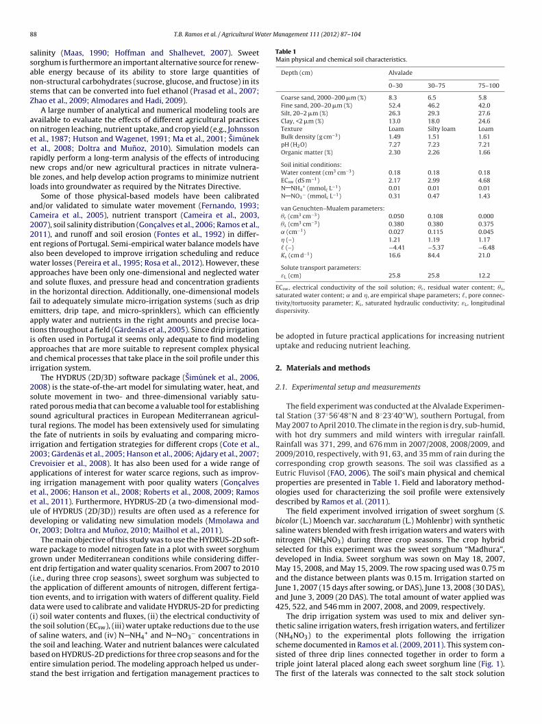
8 ater Management 111 (2012) 87– 104
ssansZ
aoeernbl
aC22eawaaifeatiaai
2srstti2CaieeudO
wge(ttd(totbes
Table 1Main physical and chemical soil characteristics.
Depth (cm) Alvalade
0–30 30–75 75–100
Coarse sand, 2000–200 �m (%) 8.3 6.5 5.8Fine sand, 200–20 �m (%) 52.4 46.2 42.0Silt, 20–2 �m (%) 26.3 29.3 27.6Clay, <2 �m (%) 13.0 18.0 24.6Texture Loam Silty loam LoamBulk density (g cm−3) 1.49 1.51 1.61pH (H2O) 7.27 7.23 7.21Organic matter (%) 2.30 2.26 1.66
Soil initial conditions:Water content (cm3 cm−3) 0.18 0.18 0.18ECsw (dS m−1) 2.17 2.99 4.68N NH4
+ (mmolc L−1) 0.01 0.01 0.01N NO3
− (mmolc L−1) 0.31 0.47 1.43
van Genuchten–Mualem parameters:�r (cm3 cm−3) 0.050 0.108 0.000�s (cm3 cm−3) 0.380 0.380 0.375˛ (cm−1) 0.027 0.115 0.045� (–) 1.21 1.19 1.17� (–) −4.41 −5.37 −6.48Ks (cm d−1) 16.6 84.4 21.0
Solute transport parameters:εL (cm) 25.8 25.8 12.2
ECsw, electrical conductivity of the soil solution; �r, residual water content; �s,saturated water content; and �, are empirical shape parameters; �, pore connec-
8 T.B. Ramos et al. / Agricultural W
alinity (Maas, 1990; Hoffman and Shalhevet, 2007). Sweetorghum is furthermore an important alternative source for renew-ble energy because of its ability to store large quantities ofon-structural carbohydrates (sucrose, glucose, and fructose) in itstems that can be converted into fuel ethanol (Prasad et al., 2007;hao et al., 2009; Almodares and Hadi, 2009).
A large number of analytical and numerical modeling tools arevailable to evaluate the effects of different agricultural practicesn nitrogen leaching, nutrient uptake, and crop yield (e.g., Johnssont al., 1987; Hutson and Wagenet, 1991; Ma et al., 2001; Simunekt al., 2008; Doltra and Munoz, 2010). Simulation models canapidly perform a long-term analysis of the effects of introducingew crops and/or new agricultural practices in nitrate vulnera-le zones, and help develop action programs to minimize nutrient
oads into groundwater as required by the Nitrates Directive.Some of those physical-based models have been calibrated
nd/or validated to simulate water movement (Fernando, 1993;ameira et al., 2005), nutrient transport (Cameira et al., 2003,007), soil salinity distribution (Gonc alves et al., 2006; Ramos et al.,011), and runoff and soil erosion (Fontes et al., 1992) in differ-nt regions of Portugal. Semi-empirical water balance models havelso been developed to improve irrigation scheduling and reduceater losses (Pereira et al., 1995; Rosa et al., 2012). However, these
pproaches have been only one-dimensional and neglected waternd solute fluxes, and pressure head and concentration gradientsn the horizontal direction. Additionally, one-dimensional modelsail to adequately simulate micro-irrigation systems (such as dripmitters, drip tape, and micro-sprinklers), which can efficientlypply water and nutrients in the right amounts and precise loca-ions throughout a field (Gärdenäs et al., 2005). Since drip irrigations often used in Portugal it seems only adequate to find modelingpproaches that are more suitable to represent complex physicalnd chemical processes that take place in the soil profile under thisrrigation system.
The HYDRUS (2D/3D) software package (Simunek et al., 2006,008) is the state-of-the-art model for simulating water, heat, andolute movement in two- and three-dimensional variably satu-ated porous media that can become a valuable tool for establishingound agricultural practices in European Mediterranean agricul-ural regions. The model has been extensively used for simulatinghe fate of nutrients in soils by evaluating and comparing micro-rrigation and fertigation strategies for different crops (Cote et al.,003; Gärdenäs et al., 2005; Hanson et al., 2006; Ajdary et al., 2007;revoisier et al., 2008). It has also been used for a wide range ofpplications of interest for water scarce regions, such as improv-ng irrigation management with poor quality waters (Gonc alvest al., 2006; Hanson et al., 2008; Roberts et al., 2008, 2009; Ramost al., 2011). Furthermore, HYDRUS-2D (a two-dimensional mod-le of HYDRUS (2D/3D)) results are often used as a reference foreveloping or validating new simulation models (Mmolawa andr, 2003; Doltra and Munoz, 2010; Mailhol et al., 2011).
The main objective of this study was to use the HYDRUS-2D soft-are package to model nitrogen fate in a plot with sweet sorghum
rown under Mediterranean conditions while considering differ-nt drip fertigation and water quality scenarios. From 2007 to 2010i.e., during three crop seasons), sweet sorghum was subjected tohe application of different amounts of nitrogen, different fertiga-ion events, and to irrigation with waters of different quality. Fieldata were used to calibrate and validate HYDRUS-2D for predictingi) soil water contents and fluxes, (ii) the electrical conductivity ofhe soil solution (ECsw), (iii) water uptake reductions due to the usef saline waters, and (iv) N NH4
+ and N NO3− concentrations in
he soil and leaching. Water and nutrient balances were calculatedased on HYDRUS-2D predictions for three crop seasons and for thentire simulation period. The modeling approach helped us under-tand the best irrigation and fertigation management practices to
tivity/tortuosity parameter; Ks, saturated hydraulic conductivity; εL, longitudinaldispersivity.
be adopted in future practical applications for increasing nutrientuptake and reducing nutrient leaching.
2. Materials and methods
2.1. Experimental setup and measurements
The field experiment was conducted at the Alvalade Experimen-tal Station (37◦56′48′′N and 8◦23′40′′W), southern Portugal, fromMay 2007 to April 2010. The climate in the region is dry, sub-humid,with hot dry summers and mild winters with irregular rainfall.Rainfall was 371, 299, and 676 mm in 2007/2008, 2008/2009, and2009/2010, respectively, with 91, 63, and 35 mm of rain during thecorresponding crop growth seasons. The soil was classified as aEutric Fluvisol (FAO, 2006). The soil’s main physical and chemicalproperties are presented in Table 1. Field and laboratory method-ologies used for characterizing the soil profile were extensivelydescribed by Ramos et al. (2011).
The field experiment involved irrigation of sweet sorghum (S.bicolor (L.) Moench var. saccharatum (L.) Mohlenbr) with syntheticsaline waters blended with fresh irrigation waters and waters withnitrogen (NH4NO3) during three crop seasons. The crop hybridselected for this experiment was the sweet sorghum “Madhura”,developed in India. Sweet sorghum was sown on May 18, 2007,May 15, 2008, and May 15, 2009. The row spacing used was 0.75 mand the distance between plants was 0.15 m. Irrigation started onJune 1, 2007 (15 days after sowing, or DAS), June 13, 2008 (30 DAS),and June 3, 2009 (20 DAS). The total amount of water applied was425, 522, and 546 mm in 2007, 2008, and 2009, respectively.
The drip irrigation system was used to mix and deliver syn-thetic saline irrigation waters, fresh irrigation waters, and fertilizer(NH4NO3) to the experimental plots following the irrigation
scheme documented in Ramos et al. (2009, 2011). This system con-sisted of three drip lines connected together in order to form atriple joint lateral placed along each sweet sorghum line (Fig. 1).The first of the laterals was connected to the salt stock solution
T.B. Ramos et al. / Agricultural Water Management 111 (2012) 87– 104 89
Fig. 1. Layout of the triple emitter source design (adapted from Ramos et al., 2009). The salt gradient decreases from sub-group A to C and the fertilizer gradient decreasesfrom group I to IV.
Table 2Discharge rates of the laterals applying salt (Na+), nitrogen (N) and fresh water (W) in each experimental plot. There is an overall constant cumulative discharge at eachdripping point of 18 L h−1 m−1 (Ramos et al., 2009).
Treatment Application rates (L h−1 m−1)
Group I Group II Group III Group IV
Na+ N W Na+ N W Na+ N W Na+ N W
1
(vat
TW
N
A 12 6 0 12 4
B 6 6 6 6 4
C 0 6 12 0 4
NaCl), while the second one was connected to the nitrogen reser-
oir. The third lateral delivered fresh water and was used to obtainconstant water application rate for each dripping point alonghe triple joint lateral (the drip discharge of 18 L h−1 m−1; which
able 3aters blended in each experimental plot during the three crop seasons.
Sub-group Irrigation water Water applied (mm)
Group I Group II
(N3) (N22007 2008 2009 2007 200
A (S2) Saline water 228.0 184.0 316.0 228.0 184Water + NH4NO3 19.3 30.0 20.0 12.9 20Fresh water 177.7 308.0 210.0 184.1 318
B (S1) Saline water 114.0 92.0 158.0 114.0 92Water + NH4NO3 19.3 30.0 20.0 12.9 20Fresh water 291.7 400.0 368.0 298.1 410
C (S0) Saline water 0.0 0.0 0.0 0.0 0Water + NH4NO3 19.3 30.0 20.0 12.9 20Fresh water 405.7 492.0 526.0 412.1 502
3, N2, N1, N0, nitrogen gradient; S2, S1, S0, salinity gradient.
2 12 2 4 12 0 68 6 2 10 6 0 124 0 2 16 0 0 18
represents 24 mm h−1 considering an area for each dripping point
of 100 cm × 75 cm). Gradients of applied salt (Na+) and nitrogen(N) concentrations were then produced by placing different emit-ters in each dripping point along the corresponding laterals andGroup III Group IV
) (N1) (N0)8 2009 2007 2008 2009 2007 2008 2009
.0 316.0 228.0 184.0 316.0 228.0 184.0 316.0
.0 13.3 6.4 10.0 6.7 0.0 0.0 0.0
.0 216.7 190.6 328.0 223.3 197.0 338.0 230.0
.0 158.0 114.0 92.0 158.0 114.0 92.0 158.0
.0 13.3 6.4 10.0 6.7 0.0 0.0 0.0
.0 374.7 304.6 420.0 381.3 311.0 430.0 388.0
.0 0.0 0.0 0.0 0.0 0.0 0.0 0.0
.0 13.3 6.4 10.0 6.7 0.0 0.0 0.0
.0 532.7 418.6 512.0 539.3 425.0 522.0 546.0
90 T.B. Ramos et al. / Agricultural Water Management 111 (2012) 87– 104
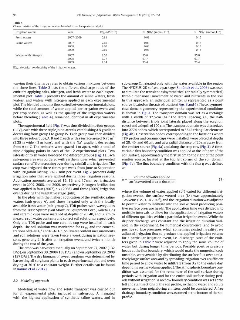
Table 4Characteristics of the irrigation waters blended in each experimental plot.
Irrigation waters Year ECiw (dS m−1) N NH4+ (mmolc L−1) N NO3
− (mmolc L−1)
Fresh waters 2007–2009 0.81 0.03 0.15
Saline waters 2007 7.60 0.03 0.152008 9.60 0.03 0.152009 10.60 0.03 0.15
Waters with nitrogen 2007 9.50 95.0 95.02008 6.77 67.7 67.72009 7.34 73.4 73.4
E
vteiwpwpbp
(di(fnlsscwiAewe
wafamOdtasd
D(hdi
2
fw
Ciw, electrical conductivity of the irrigation water.
arying their discharge rates to obtain various mixtures betweenhe three lines. Table 2 lists the different discharge rates of themitters applying salts, nitrogen, and fresh water to each exper-mental plot. Table 3 presents the amount of saline waters, fresh
aters, and waters with nitrogen applied in each experimentallot. The blended amounts thus varied between experimental plots,hile the total amount of water applied per irrigation event ander crop season, as well as the quality of the irrigation watersefore blending (Table 4), remained identical in all experimentallots.
The experimental field (Fig. 1) was thus divided into four groupsI–IV), each with three triple joint laterals, establishing a N gradientecreasing from group I to group IV. Each group was then divided
nto three sub-groups, A, B and C, each with a surface area of 6.75 m2
2.25 m wide × 3 m long), and with the Na+ gradient decreasingrom A to C. The emitters were spaced 1 m apart, with a total ofine dripping points in each of the 12 experimental plots. Two
aterals of fresh water bordered the different groups (Fig. 1). Eachub-group area was bordered with earthen ridges, which preventedurface runoff from crossing over during rainfall and irrigation. Therop was irrigated three times per week from June to Septemberith irrigation lasting 30–60 min per event. Fig. 2 presents daily
rrigation rates that were applied during three irrigation seasons.pplication amounts averaged 15, 16, and 17 mm per irrigationvent in 2007, 2008, and 2009, respectively. Nitrogen fertilizationas applied in four (2007), six (2008), and three (2009) irrigation
vents during the vegetative stage (July).In the plots with the highest application of the synthetic saline
aters (sub-group A), and those irrigated only with the locallyvailable fresh water (sub-group C), TDR probes with waveguidesrom the Trase System (Soil Moisture Equipment Corp., Goleta, CA)nd ceramic cups were installed at depths of 20, 40, and 60 cm toeasure soil water contents and collect soil solutions, respectively.nly one TDR probe and one ceramic cup were installed in eachepth. The soil solution was monitored for ECsw and the concen-rations of N NH4
+ and N NO3−. Soil water content measurements
nd soil solutions were taken twice a week during irrigation sea-ons, generally 24 h after an irrigation event, and twice a monthuring the rest of the year.
The crop was harvested manually on September 27, 2007 (132AS), on September 30, 2008 (138 DAS), and on September 29, 2009
137 DAS). The dry biomass of sweet sorghum was determined byarvesting all sorghum plants in each experimental plot and ovenrying at 70 ◦C to a constant weight. Further details can be found
n Ramos et al. (2012).
.2. Modeling approach
Modeling of water flow and solute transport was carried outor all experimental plots included in sub-group A, irrigatedith the highest application of synthetic saline waters, and in
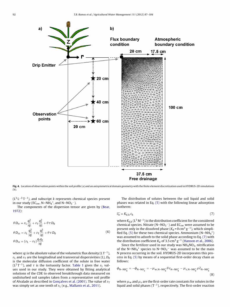
sub-group C, irrigated only with the water available in the region.The HYDRUS-2D software package (Simunek et al., 2006) was usedto simulate the transient axisymmetrical (or radially symmetrical)three-dimensional movement of water and nutrients in the soil.In this approach, an individual emitter is represented as a pointsource located on the axis of rotation (Figs. 3 and 4). The axisymmet-rical domain geometry representing the experimental conditionsis shown in Fig. 4. The transport domain was set as a rectanglewith a width of 37.5 cm (half the lateral spacing, i.e., the half-distance between triple joint laterals placed along the sorghumrows) and a depth of 100 cm. The transport domain was discretizedinto 2774 nodes, which corresponded to 5342 triangular elements(Fig. 4b). Observation nodes, corresponding to the locations whereTDR probes and ceramic cups were installed, were placed at depthsof 20, 40, and 60 cm, and at a radial distance of 20 cm away fromthe emitter source (Fig. 4a) and along the crop row (Fig. 3). A time-variable flux boundary condition was applied at the left part of thesoil surface, approximately the first 20 cm to the right of the pointemitter source, located at the top left corner of the soil domain(Fig. 4b). The flux boundary condition with the flux q was definedas:
q = volume of water appliedsurface wetted area × duration
(1)
where the volume of water applied (L3) varied for different irri-gation events, the surface wetted area (L2) was approximately1256 cm2 (i.e., 3.14 × 202), and the irrigation duration was adjustedto permit water to infiltrate into the soil without producing posi-tive surface pressure heads. The application time was divided intomultiple intervals to allow for the application of irrigation watersof different qualities within a particular irrigation event. While thedripper discharge was constant and the irrigation duration vari-able in the experiment, for numerical convenience (and to avoidpositive surface pressures, which sometimes existed in reality), weadjusted irrigation flux to produce the applied irrigation volumefor a particular irrigation event, i.e., discharge rates of the emit-ters given in Table 2 were adjusted to apply the same volume ofwater but during longer time periods. Possible positive pressureheads at the flux boundary, which would make the numerical codeunstable, were avoided by distributing the surface flux over a rela-tively large surface area and by spreading irrigation over a sufficienttime period to allow water to infiltrate (from 0.2 to the entire day,depending on the volume applied). The atmospheric boundary con-dition was assumed for the remainder of the soil surface duringperiods with irrigation and for the entire soil surface during peri-ods without irrigation. A no flow boundary condition was set at the
left and right sections of the soil profile, so that no water and solutemovement from neighboring emitters could be considered. A freedrainage boundary condition was assumed at the bottom of the soilprofile.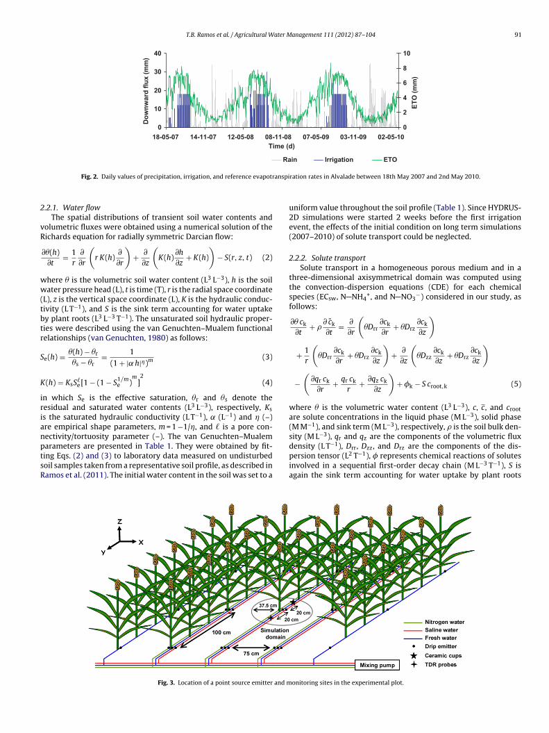
T.B. Ramos et al. / Agricultural Water Management 111 (2012) 87– 104 91
0
10
20
30
40
02-05-1003-11-0907-05-0908-11-0812-05-0814-11-0718-05-07
0
2
4
6
8
10
Rain Irrigation ETO
(d)TimeD
ow
nw
ard
flu
x (
mm
)
ET
O (
mm
)
anspi
2
vR
ww(tbtr
S
K
irianptsR
Fig. 2. Daily values of precipitation, irrigation, and reference evapotr
.2.1. Water flowThe spatial distributions of transient soil water contents and
olumetric fluxes were obtained using a numerical solution of theichards equation for radially symmetric Darcian flow:
∂�(h)∂t
= 1r
∂
∂r
(r K(h)
∂
∂r
)+ ∂
∂z
(K(h)
∂h
∂z+ K(h)
)− S(r, z, t) (2)
here � is the volumetric soil water content (L3 L−3), h is the soilater pressure head (L), t is time (T), r is the radial space coordinate
L), z is the vertical space coordinate (L), K is the hydraulic conduc-ivity (L T−1), and S is the sink term accounting for water uptakey plant roots (L3 L−3 T−1). The unsaturated soil hydraulic proper-ies were described using the van Genuchten–Mualem functionalelationships (van Genuchten, 1980) as follows:
e(h) = �(h) − �r
�s − �r= 1
(1 + | h|�)m (3)
(h) = KsS�e[1 − (1 − S1/m
e )m
]2
(4)
n which Se is the effective saturation, �r and �s denote theesidual and saturated water contents (L3 L−3), respectively, Ks
s the saturated hydraulic conductivity (L T−1), (L−1) and � (–)re empirical shape parameters, m = 1 −1/�, and � is a pore con-ectivity/tortuosity parameter (–). The van Genuchten–Mualem
arameters are presented in Table 1. They were obtained by fit-ing Eqs. (2) and (3) to laboratory data measured on undisturbedoil samples taken from a representative soil profile, as described inamos et al. (2011). The initial water content in the soil was set to aFig. 3. Location of a point source emitter and m
ration rates in Alvalade between 18th May 2007 and 2nd May 2010.
uniform value throughout the soil profile (Table 1). Since HYDRUS-2D simulations were started 2 weeks before the first irrigationevent, the effects of the initial condition on long term simulations(2007–2010) of solute transport could be neglected.
2.2.2. Solute transportSolute transport in a homogeneous porous medium and in a
three-dimensional axisymmetrical domain was computed usingthe convection-dispersion equations (CDE) for each chemicalspecies (ECsw, N NH4
+, and N NO3−) considered in our study, as
follows:
∂� ck
∂t+ �
∂ ck
∂t= ∂
∂r
(�Drr
∂ck
∂r+ �Drz
∂ck
∂z
)
+ 1r
(�Drr
∂ck
∂r+ �Drz
∂ck
∂z
)+ ∂
∂z
(�Dzz
∂ck
∂z+ �Drz
∂ck
∂z
)
−(
∂qr ck
∂r+ qr ck
r+ ∂qz ck
∂z
)+ �k − S croot,k (5)
where � is the volumetric water content (L3 L−3), c, c, and croot
are solute concentrations in the liquid phase (M L−3), solid phase(M M−1), and sink term (M L−3), respectively, � is the soil bulk den-sity (M L−3), qr and qz are the components of the volumetric flux
density (L T−1), Drr, Dzz, and Drz are the components of the dis-persion tensor (L2 T−1), � represents chemical reactions of solutesinvolved in a sequential first-order decay chain (M L−3 T−1), S isagain the sink term accounting for water uptake by plant rootsonitoring sites in the experimental plot.
92 T.B. Ramos et al. / Agricultural Water Management 111 (2012) 87– 104
F l dom(
(i
1
wεi(usuow
ig. 4. Location of observation points within the soil profile (a) and an axisymmetricab).
L3 L−3 T−1), and subscript k represents chemical species presentn our study (ECsw, N NH4
+, and N NO3−).
The components of the dispersion tensor are given by (Bear,972):
� Drr = εLq2
r|q| + εT
q2z
|q| + � D0
� Dzz = εLq2
z|q| + εT
q2r
|q| + � D0
� Drz = (εL − εT)qrqz
|q|
(6)
here |q| is the absolute value of the volumetric flux density (L T−1),L and εT are the longitudinal and transversal dispersivities (L), D0s the molecular diffusion coefficient of the solute in free waterL2 T−1), and is the tortuosity factor. Table 1 gives the εL val-es used in our study. They were obtained by fitting analytical
olutions of the CDE to observed breakthrough data measured onndisturbed soil samples taken from a representative soil profilef Alvalade as described in Gonc alves et al. (2001). The value of εTas simply set as one tenth of εL (e.g., Mallants et al., 2011).ain geometry with the finite element discretization used in HYDRUS-2D simulations
The distribution of solutes between the soil liquid and solidphases was related in Eq. (5) with the following linear adsorptionisotherm:
ck = Kd,k ck (7)
where Kd,k (L3 M−1) is the distribution coefficient for the consideredchemical species. Nitrate (N NO3
−) and ECsw were assumed to bepresent only in the dissolved phase (Kd = 0 cm3 g−1), which simpli-fied Eq. (5) for these two chemical species. Ammonium (N NH4
+)was assumed to adsorb to the solid phase according to Eq. (7) withthe distribution coefficient Kd of 3.5 cm3 g−1 (Hanson et al., 2006).
Since the fertilizer used in our study was NH4NO3, nitrificationof the N NH4
+ species to N NO3− was assumed to be the main
N process occurring in the soil. HYDRUS-2D incorporates this pro-cess in Eq. (5) by means of a sequential first-order decay chain asfollows:
�N−NH+4
= −�N−NO−3
= −w,N−NH+4
� cN−NH+4
− s,N−NH+4
� cN−NH+4
(8)
where w and s are the first-order rate constants for solutes in theliquid and solid phases (T−1), respectively. The first-order reaction
ater M
taat(
ioH
c
wruldut
2
maoS
S
wo(lpda[i
T
Te
˝
wzmroissssdatsaddGoo
T.B. Ramos et al. / Agricultural W
erms, representing nitrification of N NH4+ to N NO3
−, thus act as sink for N NH4
+ and as a source for N NO3−. The values for w
nd s were set to be 0.2 d−1. The parameters Kd, w, and s wereaken from a review of published data presented by Hanson et al.2006), and represent the center of the range of reported values.
The last term of Eq. (5) represents a passive root nutrient uptake,.e., the movement of nutrients into roots by convective mass flowf water, directly coupled with root water uptake (Simunek andopmans, 2009). This term was defined as:
root(r, z, t) = min[c(r, z, t), cmax] (9)
here cmax is the a priori defined maximum concentration of theoot solute uptake. Since we considered unlimited passive nutrientptake for nitrogen species, cmax was set to a concentration value
arger than the dissolved simulated concentrations, c, allowing allissolved nutrients to be taken up by plant roots with root waterptake. Since for ECsw a zero uptake was considered, cmax was seto zero.
.2.3. Potential and actual evapotranspiration ratesThe sink term (S) in Eqs. (2) and (5) was calculated using the
acroscopic approach introduced by Feddes et al. (1978). In thispproach, the actual local uncompensated root water uptake wasbtained as follows (Feddes et al., 1978; van Genuchten, 1987;kaggs et al., 2006a; Simunek and Hopmans, 2009):
(h, h�, r, z, t) = ˛(h, h�, r, z, t)Sp(r, z, t)
= ˛(h, h�, r, z, t)ˇ(r, z, t)Tp(t)At (10)
here Sp(r,z,t) and S(h,h� ,r,z,t) are the potential and actual volumesf water removed from a unit volume of soil per a unit of timeL3 L−3 T−1), respectively, ˛(h,h� ,r,z,t) is a prescribed dimension-ess stress response function of the soil water (h) and osmotic (h�)ressure heads (0 ≤ ≤ 1), ˇ(r,z,t) (L−3) is a normalized root densityistribution function, Tp is the potential transpiration rate (L T−1),nd At is the area of the soil surface associated with transpirationL2]. The actual transpiration rate, Ta (L T−1), was then obtained byntegrating Eq. (10) over the root domain, (L3), as follows:
a(t) = Tp(t)
∫˝r˛(h, h�, r, z, t)ˇ(r, z, t)d (11)
he root distribution is defined in HYDRUS-2D according to Vrugtt al. (2001):
(r, z) =(
1 − r
rm
) (1 − z
zm
)e−((pr/rm)|r∗−r|+(pz/zm)|z∗−z|) (12)
here rm and zm are the maximum radius and depth of the rootone (L), respectively, z* and r* are the locations of the maxi-um root water uptake in vertical and horizontal directions (L),
espectively, and the pr and pz values are taken to be equal tone except for r > r* and z > z* when they become zero. The follow-ng parameters of the Vrugt et al. (2001) model were used in theimulations: rm = 37.5 cm, zm = 65 cm, r* = 10 cm, z* = 10 cm. We con-idered a simple root distribution model in which the roots of sweetorghum expanded horizontally into all available space betweenorghum lines (rm = 37.5 cm), were concentrated mainly around therip emitter (r* = 10 cm, z* = 10 cm) where water and nutrients werepplied, and extended to a depth of 65 cm (zm = 65 cm). We assumedhat plants had no need of expanding their roots below this depthince water and nutrients were being applied at the soil surfacend their life cycle lasted only five months. The parameters forefining the maximum root water uptake in vertical and horizontal
irections (z and r*) were also based on the scenarios developed byärdenäs et al. (2005) and Hanson et al. (2006, 2008). The selectionf the maximum rooting depth was also based on the work carriedut by Ramos et al. (2011) and the fact that root depths are relativelyanagement 111 (2012) 87– 104 93
shallow under surface drip irrigation starting few days after sowing(Klepper, 1991; Allen et al., 1998; Zegada-Lizarazu et al., 2012). Inaddition, field observations carried out in November 2010 found nosignificant amounts of roots below this depth.
In this study we considered that during the growing sea-sons Tp rates were obtained by combining the daily values ofreference evapotranspiration (ET0), determined with the FAOPenman–Monteith method and the dual crop coefficient approach(Allen et al., 1998, 2005), as follows:
ETc = (Kcb + Ke)ET0 (13)
where ETc is the evapotranspiration (L T−1), Kcb is the basal cropcoefficient, which represents the plant transpiration component(–), and Ke is the soil evaporation coefficient (–).
Standard sweet sorghum Kcb values (Allen et al., 1998) wereadjusted for the Alvalade climate, taking into consideration thecrop height, wind speed, and minimum relative humidity aver-ages for the period under consideration. The Kcb coefficient wasfurther adjusted to account for the salinity and nitrogen stress,affecting sweet sorghum growth in each experimental plot, usingthe procedure for non-pristine agricultural vegetation (Allen et al.,1998):
Kcb mid = Kc min + (Kcb full − Kc min)(1 − e(−0.7 LAI)) (14)
where Kcb mid is the estimated basal Kcb during mid-season whenthe leaf area index (LAI) (L2 L−2) is smaller than for full coverconditions, Kcb full is the estimated basal Kcb during mid-season(at the peak plant size or height) for vegetation having LAI > 3,and Kc min is the minimum Kc for bare soil (0.15–0.20). For theseestimations, LAI was monitored in each experimental plot dur-ing different stages of the sorghum cycle, using a non-destructivemethod to avoid removing plants from the experimental area.Length (L) and width (W) of crop leafs were measured on randomplants grown in each experimental plot. These dimensions werethen related to previously calibrated LAI values with the followingequation:
LAI = 0.7586n∑
i=1
(L × W) (15)
where LAI are the values measured using a LI-COR areameter (Model LI-3100C, LI-COR Environmental and BiotechnologyResearch Systems, Lincoln, NE) and n is the number of green leafson each measured sorghum plant. Cubic splines were then fittedto LAI data to obtain a continuous function throughout the cropseasons.
The evaporation coefficient Ke was calculated as (Allen et al.,1998, 2005):
Ke = Kr(Kc max − Kcb) ≤ fewKc max (16)
where Kr is a dimensionless evaporation reduction coefficientdependent on the cumulative depth of water depleted (evaporated)from the topsoil, Kc max is the maximum value of Kc (i.e., Kcb + Ke)after rain or irrigation, and few is the fraction of the soil surfacefrom which most evaporation occurs. Table 5 presents the cropcoefficients and other crop related parameters estimated in eachgrowing season.
During non-growing seasons, the procedure to estimate ETc wasgreatly simplified by using the single crop coefficient approachand a Kc of 0.15 to account for a bare soil with a small percent-age of weeds. Transpiration and evaporation were also separatedas a function of leaf area index (Ritchie, 1972) using a fictitious LAI
value of 1.0.In all experimental plots, it was assumed that the potential rootwater uptake was reduced due to water stress as a result of theadopted irrigation schedule, which could lead to insufficient or
94 T.B. Ramos et al. / Agricultural Water Management 111 (2012) 87– 104
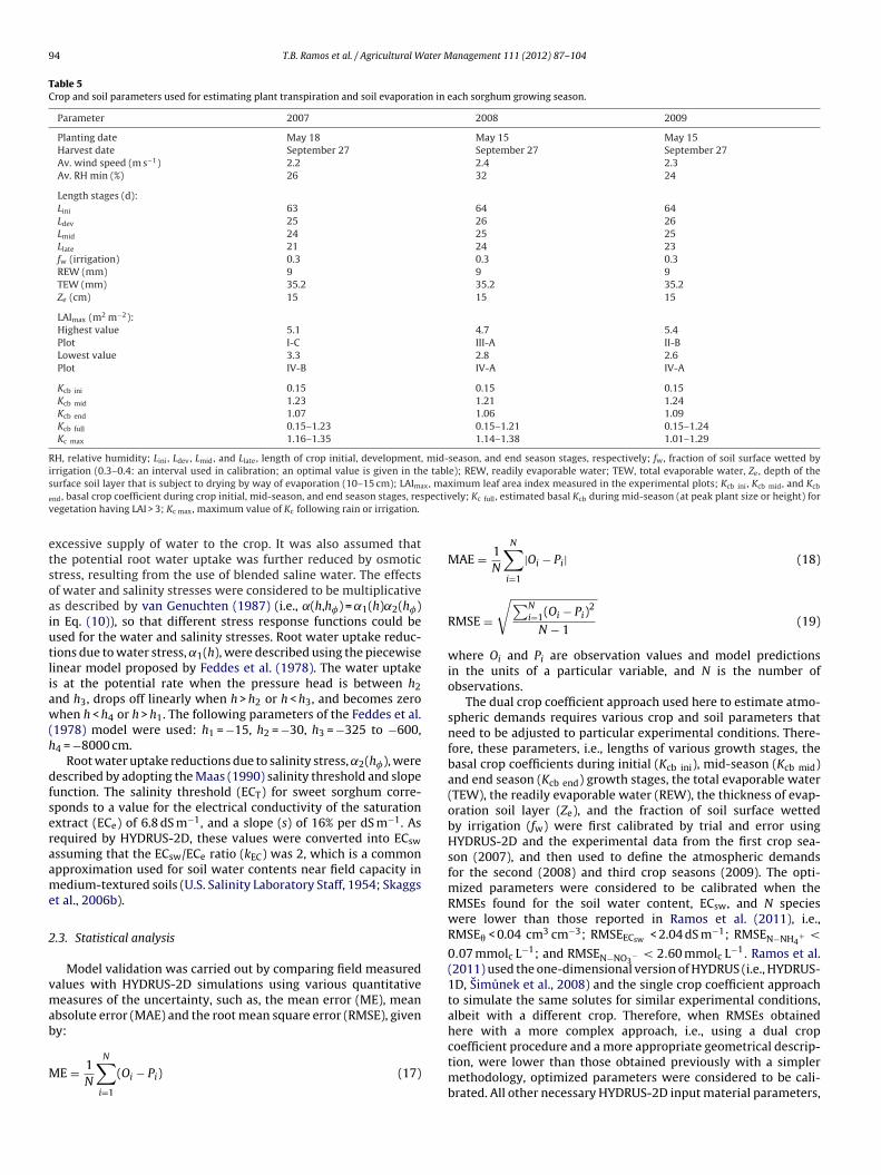
Table 5Crop and soil parameters used for estimating plant transpiration and soil evaporation in each sorghum growing season.
Parameter 2007 2008 2009
Planting date May 18 May 15 May 15Harvest date September 27 September 27 September 27Av. wind speed (m s−1) 2.2 2.4 2.3Av. RH min (%) 26 32 24
Length stages (d):Lini 63 64 64Ldev 25 26 26Lmid 24 25 25Llate 21 24 23fw (irrigation) 0.3 0.3 0.3REW (mm) 9 9 9TEW (mm) 35.2 35.2 35.2Ze (cm) 15 15 15
LAImax (m2 m−2):Highest value 5.1 4.7 5.4Plot I-C III-A II-BLowest value 3.3 2.8 2.6Plot IV-B IV-A IV-A
Kcb ini 0.15 0.15 0.15Kcb mid 1.23 1.21 1.24Kcb end 1.07 1.06 1.09Kcb full 0.15–1.23 0.15–1.21 0.15–1.24Kc max 1.16–1.35 1.14–1.38 1.01–1.29
RH, relative humidity; Lini , Ldev, Lmid, and Llate, length of crop initial, development, mid-season, and end season stages, respectively; fw, fraction of soil surface wetted byirrigation (0.3–0.4: an interval used in calibration; an optimal value is given in the table); REW, readily evaporable water; TEW, total evaporable water, Ze, depth of thes x, mae pectivv
etsoaiutliaw(h
dfseraame
2
vmab
M
urface soil layer that is subject to drying by way of evaporation (10–15 cm); LAIma
nd, basal crop coefficient during crop initial, mid-season, and end season stages, resegetation having LAI > 3; Kc max, maximum value of Kc following rain or irrigation.
xcessive supply of water to the crop. It was also assumed thathe potential root water uptake was further reduced by osmotictress, resulting from the use of blended saline water. The effectsf water and salinity stresses were considered to be multiplicatives described by van Genuchten (1987) (i.e., ˛(h,h�) = ˛1(h)˛2(h�)n Eq. (10)), so that different stress response functions could besed for the water and salinity stresses. Root water uptake reduc-ions due to water stress, ˛1(h), were described using the piecewiseinear model proposed by Feddes et al. (1978). The water uptakes at the potential rate when the pressure head is between h2nd h3, drops off linearly when h > h2 or h < h3, and becomes zerohen h < h4 or h > h1. The following parameters of the Feddes et al.
1978) model were used: h1 = −15, h2 = −30, h3 = −325 to −600,4 = −8000 cm.
Root water uptake reductions due to salinity stress, ˛2(h�), wereescribed by adopting the Maas (1990) salinity threshold and slopeunction. The salinity threshold (ECT) for sweet sorghum corre-ponds to a value for the electrical conductivity of the saturationxtract (ECe) of 6.8 dS m−1, and a slope (s) of 16% per dS m−1. Asequired by HYDRUS-2D, these values were converted into ECsw
ssuming that the ECsw/ECe ratio (kEC) was 2, which is a commonpproximation used for soil water contents near field capacity inedium-textured soils (U.S. Salinity Laboratory Staff, 1954; Skaggs
t al., 2006b).
.3. Statistical analysis
Model validation was carried out by comparing field measuredalues with HYDRUS-2D simulations using various quantitativeeasures of the uncertainty, such as, the mean error (ME), mean
bsolute error (MAE) and the root mean square error (RMSE), giveny:
E = 1N
N∑i=1
(Oi − Pi) (17)
ximum leaf area index measured in the experimental plots; Kcb ini , Kcb mid, and Kcb
ely; Kc full , estimated basal Kcb during mid-season (at peak plant size or height) for
MAE = 1N
N∑i=1
|Oi − Pi| (18)
RMSE =√∑N
i=1(Oi − Pi)2
N − 1(19)
where Oi and Pi are observation values and model predictionsin the units of a particular variable, and N is the number ofobservations.
The dual crop coefficient approach used here to estimate atmo-spheric demands requires various crop and soil parameters thatneed to be adjusted to particular experimental conditions. There-fore, these parameters, i.e., lengths of various growth stages, thebasal crop coefficients during initial (Kcb ini), mid-season (Kcb mid)and end season (Kcb end) growth stages, the total evaporable water(TEW), the readily evaporable water (REW), the thickness of evap-oration soil layer (Ze), and the fraction of soil surface wettedby irrigation (fw) were first calibrated by trial and error usingHYDRUS-2D and the experimental data from the first crop sea-son (2007), and then used to define the atmospheric demandsfor the second (2008) and third crop seasons (2009). The opti-mized parameters were considered to be calibrated when theRMSEs found for the soil water content, ECsw, and N specieswere lower than those reported in Ramos et al. (2011), i.e.,RMSE� < 0.04 cm3 cm−3; RMSEECsw < 2.04 dS m−1; RMSEN−NH4
+ <
0.07 mmolc L−1; and RMSEN−NO3− < 2.60 mmolc L−1. Ramos et al.
(2011) used the one-dimensional version of HYDRUS (i.e., HYDRUS-1D, Simunek et al., 2008) and the single crop coefficient approachto simulate the same solutes for similar experimental conditions,albeit with a different crop. Therefore, when RMSEs obtainedhere with a more complex approach, i.e., using a dual crop
coefficient procedure and a more appropriate geometrical descrip-tion, were lower than those obtained previously with a simplermethodology, optimized parameters were considered to be cali-brated. All other necessary HYDRUS-2D input material parameters,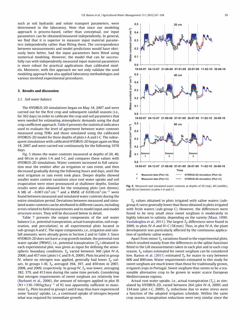
ater Management 111 (2012) 87– 104 95
sdapwtbonfiemv
3
3
cfwcumHq1d
aHtdnserAfeles
bosfHwes2Iu23t((msw
Time
Wate
rc
on
ten
t(c
m3
cm
-3)
Wate
rc
on
ten
t(c
m3
cm
-3)
Wate
rc
on
ten
t(c
m3
cm
-3)
Measured data (Plot I-A)
Measured data (Plot I-C)
HYDR US-2D simulation (Plot I-A)
HYDR US-2D simulation (Plot I-C )
0.0
0.1
0.2
0.3
0.4
0.5
18-05 -07 04 -12 -07 21 -06 -08 07-01-09 26 -07 -09 11 -02 -10 30 -08 -10
0.0
0.1
0.2
0.3
0.4
0.5
18-05 -07 04 -12 -07 21 -06 -08 07 -01 -09 26 -07 -09 11 -02-10 30 -08 -10
0.0
0.1
0.2
0.3
0.4
0.5
18-05 -07 04 -12 -07 21-06-08 07 -01 -09 26 -07 -09 11-02-10 30 -08 -10
20 cm
40 cm
60 cm
Season
1
Season
2
Season
3
T.B. Ramos et al. / Agricultural W
uch as soil hydraulic and solute transport parameters, wereetermined in the laboratory. Note that since our modelingpproach is process-based, rather than conceptual, our inputarameters can be obtained/measured independently. In general,e find that it is superior to measure input material parame-
ers independently rather than fitting them. The correspondenceetween measurements and model predictions would have obvi-usly been better, had the input parameters been fitted usingumerical modeling. However, the model that can be success-
ully run with independently measured input material parameterss more robust for practical applications than calibrated mod-ls. Moreover, with this approach we not only validate the usedodeling approach but also applied laboratory methodologies and
arious involved experimental procedures.
. Results and discussion
.1. Soil water balance
The HYDRUS-2D simulations began on May 18, 2007 and werearried out for the first crop and subsequent rainfall seasons (i.e.,or 362 days) in order to calibrate the crop and soil parameters thatere needed for estimating atmospheric demands using the dual
rop coefficient approach. Table 6 presents the statistical indicatorssed to evaluate the level of agreement between water contentseasured using TDRs and those simulated using the calibratedYDRUS-2D model for three depths of plots I-A and I-C. The subse-uent simulations with calibrated HYDRUS-2D began again on May8, 2007 and were carried out continuously for the following 1078ays.
Fig. 5 shows the water contents measured at depths of 20, 40,nd 60 cm in plots I-A and I-C, and compares these values withYDRUS-2D simulations. Water contents increased to full satura-
ion near the emitter after an irrigation or rain event, and thenecreased gradually during the following hours and days, until theext irrigation or rain event took place. Deeper depths showedmaller water content variations since root water uptake and soilvaporation were more pronounced at shallower depths. Similaresults were also obtained for the remaining plots (not shown).
ME of −0.007 cm3 cm−3 and a RMSE of 0.030 cm3 cm−3 wereound between measured and simulated water contents during thentire simulation period. Deviations between measured and simu-ated water contents can be attributed to different causes, includingrrors related to field measurements and to model input and modeltructure errors. They will be discussed below in detail.
Table 7 presents the output components of the soil wateralance (i.e., potential transpiration, actual transpiration, soil evap-ration, and percolation) in all experimental plots located inub-groups A and C. The input components, i.e., irrigation and rain-all amounts, were already given in Section 2 and in Table 3. SinceYDRUS-2D does not have a crop growth module, the potential rootater uptake (PRWU), i.e., potential transpiration (Tp) obtained in
ach experimental plot, was given as input for defining the atmo-pheric boundary conditions. Tp varied between 360 (plot IV-A,008) and 457 mm (plots I-C and II-A, 2009). Plots located in group
V, where no nitrogen was applied, generally had lower Tp val-es. In groups I–III, Tp averaged 394, 397, and 450 mm in 2007,008, and 2009, respectively. In group IV, Tp was lower, averaging82, 379, and 413 mm during the same time periods. Consideringhat nitrogen requirements of sweet sorghum are relatively lowBarbanti et al., 2006), the amount of nitrogen applied in plot III
N1 = 130–190 kg/ha y−1 of N) was apparently sufficient to maxi-ize Tp. Plots located in groups I and II may thus have experiencedome ‘luxury’ uptake, i.e., a continued uptake of nitrogen beyondhat was required for immediate growth.
Fig. 5. Measured and simulated water contents at depths of 20 (top), 40 (middle),and 60 cm (bottom) in plots I-A and I-C.
Tp values obtained in plots irrigated with saline waters (sub-group A) were generally lower that those obtained in plots irrigatedwith fresh waters (sub-group C). However, the differences werefound to be very small since sweet sorghum is moderately tohighly tolerant to salinity, depending on the variety (Maas, 1990;Vasilakoglou et al., 2011). The largest Tp differences were found in2009, in plots IV-A and IV-C (58 mm). Thus, in plot IV-A, the plantdevelopment was particularly affected by the continuous applica-tion of synthetic saline waters.
Apart from minor Tp variations found in the experimental plots,which resulted mainly from the differences in the spline functionsfitted to the LAI measurements taken in each plot and in each cropseason, Tp values estimated for sweet sorghum can be consideredlow. Ramos et al. (2011) estimated Tp for maize to vary between600 and 800 mm. Water requirements estimated in this study forsweet sorghum are much lower than those for traditionally grown,irrigated crops in Portugal. Sweet sorghum thus seems to be a rea-sonable alternative crop to be grown in water scarce EuropeanMediterranean regions.
Actual root water uptake, i.e., actual transpiration (Ta), as sim-
ulated by HYDRUS-2D, varied between 264 (plot IV-A, 2009) and334 mm (plot I-C, 2009). Tp reductions due to water stress werea function of the adopted irrigation schedule. Within the samecrop season, transpiration reductions were very similar since the
96 T.B. Ramos et al. / Agricultural Water Management 111 (2012) 87– 104
Table 6Results of the statistical analysis between measured and simulated soil water contents, electrical conductivities of the soil solution (ECsw), and N NH4
+, and N NO3−
concentrations.
Statistic Water content (cm3 cm−3) ECsw (dS m−1) N NH4+ (mmolc L−1) N NO3
− (mmolc L−1)
Data from 2007/2008 (calibration data):N 82 36 93 75ME −0.007 −0.216 0.029 −0.218MAE 0.024 0.602 0.029 0.617RMSE 0.033 0.854 0.042 1.253
Data from 2008/2010:N 276 211 241 263ME −0.007 −0.668 0.019 −1.668MAE 0.023 1.255 0.026 2.244RMSE 0.028 1.877 0.043 3.427
Data from 2007/2010 (all data):N 358 247 334 338ME −0.007 −0.602 0.022 −1.346MAE 0.023 1.160 0.027 1.883RMSE 0.030 1.764
N, number of observations; ME, mean error; MAE, mean absolute error; RMSE, root mean
y = 198.83x - 41438.86
R2 = 0.51
5000
10000
15000
20000
25000
30000
350330310290270250
Ta (mm)
Dry
bio
ma
ss
(k
g/h
a)
Csub-groupdata fromAsub-groupdata from
Fa
ipw2ts
Teiirffrstwtica
2iYls
plots I-A and I-C, and compares these values with HYDRUS-2D sim-
ig. 6. Relationship between actual transpiration (Ta), as simulated by HYDRUS-2D,nd dry biomass yield (Y).
rrigation schedule was the same in all experimental plots. In thelots located in sub-group C, irrigated only with fresh waters, Tp
as reduced due to water stress by 25.3–27.4%, 21.9–22.8%, and6.3–26.9% in 2007, 2008, and 2009, respectively. Water stress washus a function of the adopted irrigation schedule during each sea-on and did not vary among experimental plots.
In plots located in sub-group A (irrigated with saline waters),p was further reduced due to salinity stress. During 2007, Ta
stimated for the different plots included in sub-group A was gener-cally the same as in sub-group C (irrigated with fresh waters),.e., sweet sorghum showed to be tolerant to the levels of salinityeached in the soil solution of all experimental plots irrigated withresh or synthetic saline waters. However, in 2008 and 2009, Tp suf-ered reductions (in sub-group A) of 24.2–26.9%, and 31.3–33.3%,espectively, due to the combined effects of water and salinitytresses, i.e., 2.3–4.7% (in 2008) and 4.6–7.0% (in 2009) higherhan Tp reductions found in the plots irrigated only with freshaters (sub-group C). In the following years, the salinity stress
hus became increasingly higher (in sub-group A). Hence, soil salin-zation and the increase of the salinity stress was related to theontinuous and increasing amount of synthetic saline waters beingpplied in each experimental plot.
Fig. 6 relates actual transpiration Ta calculated using HYDRUS-D with the experimentally determined sorghum yield (Y), given
n terms of dry biomass, by means of the empirical relationship,
= f (Ta). This relationship, generally thought to be approximatelyinear, is valid for a particular plant (canopy) at a particular siteubject to standard tillage and nutrition conditions (Novák and van
0.042 3.078
square error.
Genuchten, 2008). The relation found in our study was somewhatpoor, with the agreement between Ta and dry biomass reaching R2
of only 0.51. Since HYDRUS-2D does not account for a crop growthmodule, this result was not particularly surprising. Nevertheless,had water been the only limiting factor in our experiment, the rela-tion would likely have been better. However, this could not be easilyobserved in our study since the amount of water applied per yearwas the same, while the total water depths applied during each cropseason were apparently not different enough to establish a closerrelation. The relation in Fig. 6 essentially resulted from the effectsthat water quality had on Ta and crop yield. While plots irrigatedwith fresh water (sub-group C) had higher sorghum yields and Ta
values, plots irrigated with saline waters (sub-group A) had lowersorghum yields and Ta values (Fig. 6). Nitrogen also did not influ-ence the Y(Ta) relation since N stress at a given period can mainlyaffect sorghum yield, while LAI, and consequently Ta, remain high.
Finally, the soil water balance (Table 7) in each experimen-tal plot shows relatively high percolation. Percolation reached162–174, 292–299, and 292–309 mm in 2007, 2008, and 2009,respectively. These values correspond to 31–34%, 50–51%, and51–54% of the water applied during crop seasons, i.e., from sow-ing to harvest. While percolation was expected to be large, sinceapplication rates during irrigation seasons were high, the valuesestimated for crop seasons of 2008 and 2009 may be somewhatdeceiving. They result from running HYDRUS-2D continuously forthe entire simulation period. Since cumulative percolation obtainedduring the entire simulation period (2007–2010) only reached36–37% of the applied water, and considering that root wateruptake was much higher during crop seasons, percolation in 2008and 2009 also accounted for the water stored below the root zone.Therefore, we ended up not being able to actually quantify per-colation due to the adopted irrigation schedule, since the waterbalance evaluated for each crop season also accounted for thewater that was no longer accessible to plants. Nevertheless, theeffects of nitrogen applications and water quality on drainage weresmall. Plots with higher root water uptake showed generally lowerpercolation.
3.2. Salinity build-up and distribution
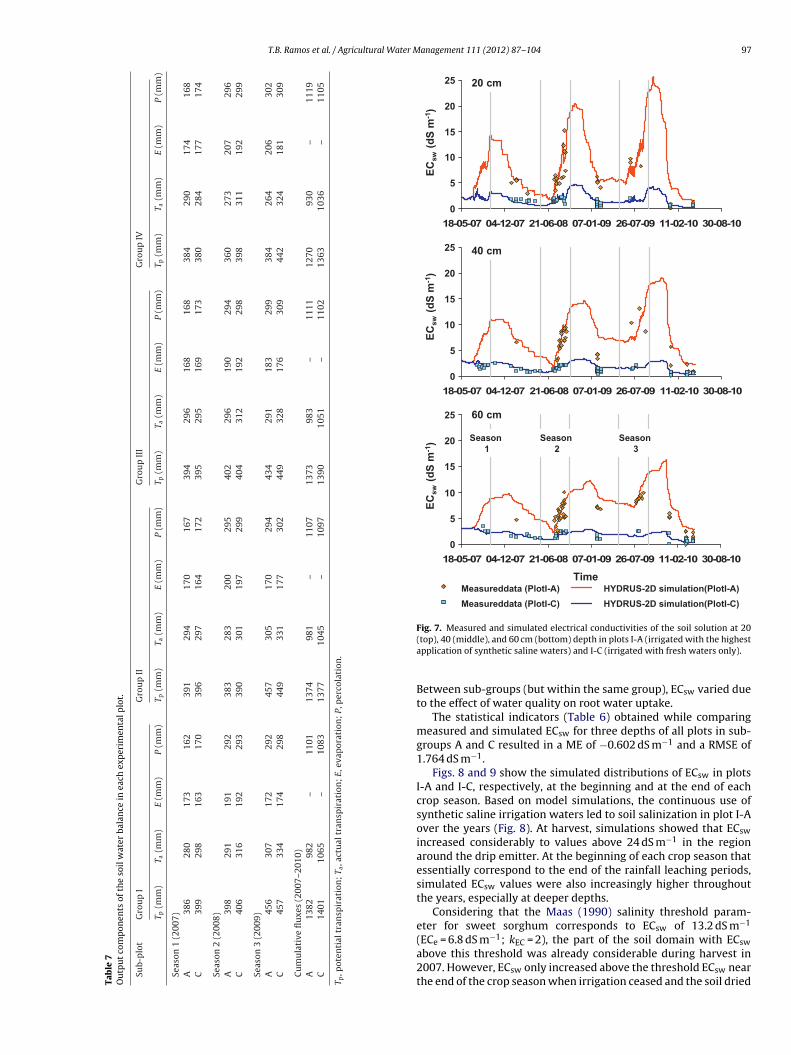
Fig. 7 shows ECsw measured at the 20, 40, and 60 cm depth in
ulations. Similar results were also found for the remaining plots ofsub-groups A and C. Within the same sub-group (Fig. 1), ECsw var-ied due to the effect of nitrogen fertigation on root water uptake.
T.B. Ramos et al. / Agricultural Water Management 111 (2012) 87– 104 97
Tab
le
7O
utp
ut
com
pon
ents
of
the
soil
wat
er
bala
nce
in
each
exp
erim
enta
l plo
t.
Sub-
plo
tG
rou
p
I
Gro
up
II
Gro
up
III
Gro
up
IV
T p(m
m)
T a(m
m)
E
(mm
)
P
(mm
)
T p(m
m)
T a(m
m)
E
(mm
)
P
(mm
)
T p(m
m)
T a(m
m)
E
(mm
)
P
(mm
)
T p(m
m)
T a(m
m)
E (m
m)
P
(mm
)
Seas
on
1
(200
7)A
386
280
173
162
391
294
170
167
394
296
168
168
384
290
174
168
C39
929
816
317
0
396
297
164
172
395
295
169
173
380
284
177
174
Seas
on
2
(200
8)A
398
291
191
292
383
283
200
295
402
296
190
294
360
273
207
296
C40
631
619
229
339
030
119
729
940
4
312
192
298
398
311
192
299
Seas
on
3
(200
9)A
456
307
172
292
457
305
170
294
434
291
183
299
384
264
206
302
C
457
334
174
298
449
331
177
302
449
328
176
309
442
324
181
309
Cu
mu
lati
ve
flu
xes
(200
7–20
10)
A13
82
982
–
1101
1374
981
–
1107
1373
983
–
1111
1270
930
–
1119
C
1401
1065
–
1083
1377
1045
–
1097
1390
1051
–
1102
1363
1036
–
1105
T p, p
oten
tial
tran
spir
atio
n;
T a, a
ctu
al
tran
spir
atio
n;
E,
evap
orat
ion
;
P,
per
cola
tion
.
0
5
10
15
20
25
18-05 -07 04-12 -07 21-06 -08 07-01 -09 26-07 -09 11-02 -10 30-08 -10
0
5
10
15
20
25
18-05 -07 04-12 -07 21-06 -08 07-01 -09 26-07 -09 11-02 -10 30 -08 -10
0
5
10
15
20
25
18-05 -07 04-12-07 21-06-08 07 -01-09 26 -07-09 11 -02 -10 30 -08 -10
Time
EC
sw
(dS
m-1
)
Measureddata (PlotI-A)
Measureddata (PlotI-C)
HYDRUS-2D simulation(PlotI-A)
HYDRUS-2D simulation(PlotI-C)
Season
1
Season
2
Season
3
EC
sw
(dS
m-1
)E
Csw
(dS
m-1
)60 cm
40 cm
20 cm
Fig. 7. Measured and simulated electrical conductivities of the soil solution at 20
(top), 40 (middle), and 60 cm (bottom) depth in plots I-A (irrigated with the highestapplication of synthetic saline waters) and I-C (irrigated with fresh waters only).Between sub-groups (but within the same group), ECsw varied dueto the effect of water quality on root water uptake.
The statistical indicators (Table 6) obtained while comparingmeasured and simulated ECsw for three depths of all plots in sub-groups A and C resulted in a ME of −0.602 dS m−1 and a RMSE of1.764 dS m−1.
Figs. 8 and 9 show the simulated distributions of ECsw in plotsI-A and I-C, respectively, at the beginning and at the end of eachcrop season. Based on model simulations, the continuous use ofsynthetic saline irrigation waters led to soil salinization in plot I-Aover the years (Fig. 8). At harvest, simulations showed that ECsw
increased considerably to values above 24 dS m−1 in the regionaround the drip emitter. At the beginning of each crop season thatessentially correspond to the end of the rainfall leaching periods,simulated ECsw values were also increasingly higher throughoutthe years, especially at deeper depths.
Considering that the Maas (1990) salinity threshold param-eter for sweet sorghum corresponds to ECsw of 13.2 dS m−1
(EC = 6.8 dS m−1; k = 2), the part of the soil domain with EC
e EC swabove this threshold was already considerable during harvest in2007. However, ECsw only increased above the threshold ECsw nearthe end of the crop season when irrigation ceased and the soil dried

98 T.B. Ramos et al. / Agricultural Water Management 111 (2012) 87– 104
Fig. 8. Simulated distributions of the electrical conductivity of the soil solution inplot I-A (irrigated with synthetic saline waters) during sowing (top) and harvest(e
od2amrs
tetia
3
apscIiscw
Fig. 9. Simulated distributions of the electrical conductivity of the soil solution in
due to rapid nitrification, it does not stay long enough in the root
bottom) of each crop season. The drip emitter was located in the top left corner ofach contour plot.
ut (Fig. 7). Therefore, transpiration was not significantly reducedue to the salinity stress during that year (Table 7). In 2008 and009, the threshold value was reached earlier, with the regionround the drip emitter with ECsw values above 13.2 dS m−1 beinguch larger than in 2007. Hence, transpiration was increasingly
educed due to the salinity stress as a result of the accumulation ofalts in the soil domain.
On the other hand, irrigation with fresh waters, having a rela-ively low salinity (ECiw > 0.8; Table 4), also led to larger ECsw at thend of each crop season, but the levels reached were always lowerhan 9 dS m−1 and decreased significantly due to rainfall leach-ng (Fig. 9). Therefore, in sub-group C, root water uptake was notffected by the salinity stress.
.3. Nitrogen balance
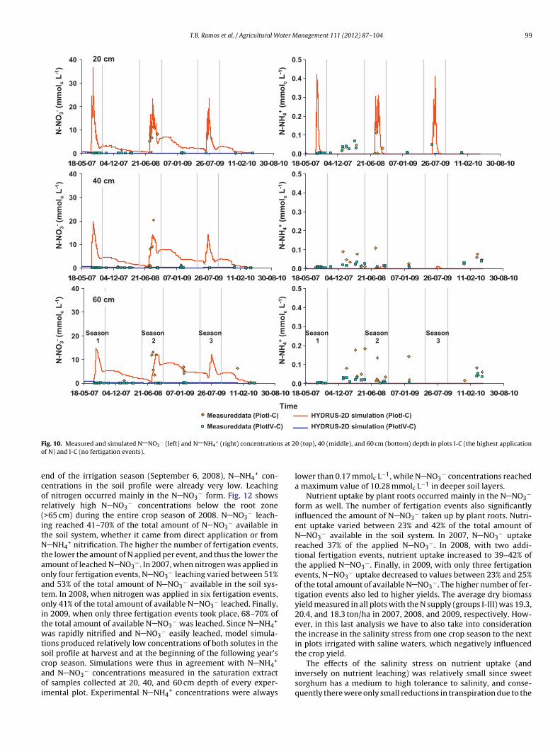
Fig. 10 shows N NH4+ and N NO3
− concentrations measuredt a depth of 20, 40, and 60 cm in plots I-C and IV-C, and com-ares these values with HYDRUS-2D simulations. Figs. 11 and 12how the simulated distributions of N NH4
+ and N NO3− con-
entrations in plot I-A during the second crop season. In groups through IV, N NH4
+ and N NO3− concentrations varied accord-
ng to the amounts of nitrogen applied in each experimental plot. In
ub-group A-C (but within the same group), N NH4+ and N NO3−
oncentrations varied due to the effects of water quality on rootater uptake.
plot I-C (irrigated with fresh waters only) during sowing (top) and harvest (bottom)of each crop season. The drip emitter was located in the top left corner of eachcontour plot.
The statistical indicators (Table 6) obtained while compar-ing measured and simulated N NH4
+ concentrations for threedepths, and for all experimental plots located in sub-groupsA and C, showed a ME of 0.022 mmolc L−1 and a RMSE of0.042 mmolc L−1. Corresponding statistical indicators for N NO3
−
concentrations resulted in a ME of −1.346 mmolc L−1 and a RMSEof 3.078 mmolc L−1.
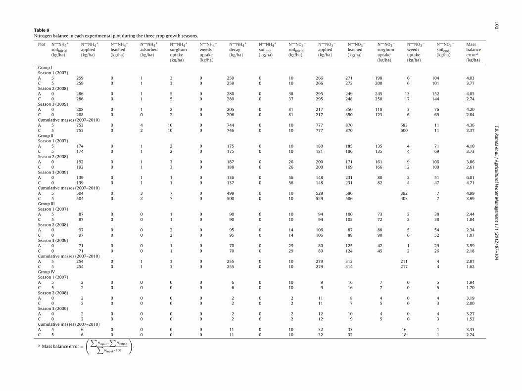
Table 8 shows the nitrogen balances evaluated for each exper-imental plot during the three crop seasons included in thesimulation period. While most components of the nitrogen balancewere restricted to the duration of a crop season, leaching was cal-culated to also include the solute mass lost during the subsequentrainfall period. Nitrogen leaching was directly related to water flowthrough the bottom boundary of the soil domain. Therefore, sincethe percolation component of the water balance was high, so wasthe nitrogen leaching component here. The movement of N out ofthe root zone also depended on the amount of applied N, the formof N in the fertilizer, and the time and number of fertigation events.
Based on model simulations, most of the applied N NH4+ was
rapidly nitrified into N NO3−, not reaching depths deeper than
20 cm and not being significantly taken up by plant roots. On the onehand, N NH4
+ adsorbs to the solid phase and thus its movement issignificantly retarded compared to N NO3
−, and on the other hand,
zone to be taken up by plant roots. Fig. 11 exemplifies how, basedon model simulations, N NH4
+ concentrations never increased atdepths below 20 cm during the crop season of 2008. Also, at the
T.B. Ramos et al. / Agricultural Water Management 111 (2012) 87– 104 99
0
10
20
30
40
18-05-07 04 -12-07 21-06-08 07-01-09 26 -07-09 11-02-10 30 -08-10
0
10
20
30
40
18-05-07 04 -12-07 21-06-08 07-01 -09 26-07-09 11-02-10 30 -08-10
0.0
0.1
0.2
0.3
0.4
0.5
18-05-07 04-12-07 21-06 -08 07-01-09 26-07-09 11-02-10 30 -08-10
0.0
0.1
0.2
0.3
0.4
0.5
18-05-07 04-12 -07 21-06 -08 07-01-09 26-07-09 11-02 -10 30 -08-10
0.0
0.1
0.2
0.3
0.4
0.5
18-05-07 04-12-07 21-06-08 07-01-09 26-07-09 11-02-10 30-08-10
TimeMeasureddata (PlotI-C)
Measureddata (PlotIV-C)
HYDRUS-2D simulation (PlotI-C)
HYDRUS-2D simulation (PlotIV-C)
0
10
20
30
40
18-05-07 04 -12-07 21-06-08 07 -01-09 26-07-09 11-02-10 30-08-10
N-N
O3-(m
mo
l cL
-1)
N-N
H4+
(mm
ol c
L-1
)
N-N
O3-(m
mo
l cL
-1)
N-N
H4+
(mm
ol c
L-1
)
N-N
O3-(m
mo
l cL
-1)
N-N
H4+
(mm
ol c
L-1
)
Season
1
Season
2
Season
3
Season
1
Season
2
Season
3
60 cm
40 cm
20 cm
F s at 2o
ecor(itNtaoatoitwtscaoi
ig. 10. Measured and simulated N NO3− (left) and N NH4
+ (right) concentrationf N) and I-C (no fertigation events).
nd of the irrigation season (September 6, 2008), N NH4+ con-
entrations in the soil profile were already very low. Leachingf nitrogen occurred mainly in the N NO3
− form. Fig. 12 showselatively high N NO3
− concentrations below the root zone>65 cm) during the entire crop season of 2008. N NO3
− leach-ng reached 41–70% of the total amount of N NO3
− available inhe soil system, whether it came from direct application or from
NH4+ nitrification. The higher the number of fertigation events,
he lower the amount of N applied per event, and thus the lower themount of leached N NO3
−. In 2007, when nitrogen was applied innly four fertigation events, N NO3
− leaching varied between 51%nd 53% of the total amount of N NO3
− available in the soil sys-em. In 2008, when nitrogen was applied in six fertigation events,nly 41% of the total amount of available N NO3
− leached. Finally,n 2009, when only three fertigation events took place, 68–70% ofhe total amount of available N NO3
− was leached. Since N NH4+
as rapidly nitrified and N NO3− easily leached, model simula-
ions produced relatively low concentrations of both solutes in theoil profile at harvest and at the beginning of the following year’s
rop season. Simulations were thus in agreement with N NH4+
nd N NO3− concentrations measured in the saturation extract
f samples collected at 20, 40, and 60 cm depth of every exper-mental plot. Experimental N NH4
+ concentrations were always
0 (top), 40 (middle), and 60 cm (bottom) depth in plots I-C (the highest application
lower than 0.17 mmolc L−1, while N NO3− concentrations reached
a maximum value of 10.28 mmolc L−1 in deeper soil layers.Nutrient uptake by plant roots occurred mainly in the N NO3
−
form as well. The number of fertigation events also significantlyinfluenced the amount of N NO3
− taken up by plant roots. Nutri-ent uptake varied between 23% and 42% of the total amount ofN NO3
− available in the soil system. In 2007, N NO3− uptake
reached 37% of the applied N NO3−. In 2008, with two addi-
tional fertigation events, nutrient uptake increased to 39–42% ofthe applied N NO3
−. Finally, in 2009, with only three fertigationevents, N NO3
− uptake decreased to values between 23% and 25%of the total amount of available N NO3
−. The higher number of fer-tigation events also led to higher yields. The average dry biomassyield measured in all plots with the N supply (groups I-III) was 19.3,20.4, and 18.3 ton/ha in 2007, 2008, and 2009, respectively. How-ever, in this last analysis we have to also take into considerationthe increase in the salinity stress from one crop season to the nextin plots irrigated with saline waters, which negatively influencedthe crop yield.
The effects of the salinity stress on nutrient uptake (andinversely on nutrient leaching) was relatively small since sweetsorghum has a medium to high tolerance to salinity, and conse-quently there were only small reductions in transpiration due to the
100T.B.
Ram
os et
al. /
Agricultural
Water
Managem
ent 111 (2012) 87– 104
Table 8Nitrogen balance in each experimental plot during the three crop growth seasons.
Plot N NH4+
soilInitial(kg/ha)
N NH4+
applied(kg/ha)
N NH4+
leached(kg/ha)
N NH4+
adsorbed(kg/ha)
N NH4+
sorghumuptake(kg/ha)
N NH4+
weedsuptake(kg/ha)
N NH4+
decay(kg/ha)
N NH4+
soilend(kg/ha)
N NO3−
soilInitial(kg/ha)
N NO3−
applied(kg/ha)
N NO3−
leached(kg/ha)
N NO3−
sorghumuptake(kg/ha)
N NO3−
weedsuptake(kg/ha)
N NO3−
soilend(kg/ha)
Massbalanceerrora
(kg/ha)
Group ISeason 1 (2007)A 5 259 0 1 3 0 259 0 10 266 271 198 6 104 4.03C 5 259 0 1 3 0 259 0 10 266 272 200 6 101 3.77Season 2 (2008)A 0 286 0 1 5 0 280 0 38 295 249 245 13 152 4.05C 0 286 0 1 5 0 280 0 37 295 248 250 17 144 2.74Season 3 (2009)A 0 208 0 1 2 0 205 0 81 217 350 118 3 76 4.20C 0 208 0 0 2 0 206 0 81 217 350 123 6 69 2.84Cumulative masses (2007–2010)A 5 753 0 4 10 0 744 0 10 777 870 583 11 4.36C 5 753 0 2 10 0 746 0 10 777 870 600 11 3.37Group IISeason 1 (2007)A 5 174 0 1 2 0 175 0 10 180 185 135 4 71 4.10C 5 174 0 1 2 0 175 0 10 181 186 135 4 69 3.73Season 2 (2008)A 0 192 0 1 3 0 187 0 26 200 171 161 9 106 3.86C 0 192 0 1 3 0 188 0 26 200 169 166 12 100 2.61Season 3 (2009)A 0 139 0 1 1 0 136 0 56 148 231 80 2 51 6.01C 0 139 0 1 1 0 137 0 56 148 231 82 4 47 4.71Cumulative masses (2007–2010)A 5 504 0 3 7 0 499 0 10 528 586 392 7 4.99C 5 504 0 2 7 0 500 0 10 529 586 403 7 3.99Group IIISeason 1 (2007)A 5 87 0 0 1 0 90 0 10 94 100 73 2 38 2.44C 5 87 0 0 1 0 90 0 10 94 102 72 2 38 1.84Season 2 (2008)A 0 97 0 0 2 0 95 0 14 106 87 88 5 54 2.34C 0 97 0 0 2 0 95 0 14 106 88 90 6 52 1.07Season 3 (2009)A 0 71 0 0 1 0 70 0 29 80 125 42 1 29 3.59C 0 71 0 0 1 0 70 0 29 80 124 45 2 26 2.18Cumulative masses (2007–2010)A 5 254 0 1 3 0 255 0 10 279 312 211 4 2.87C 5 254 0 1 3 0 255 0 10 279 314 217 4 1.62Group IVSeason 1 (2007)A 5 2 0 0 0 0 6 0 10 9 16 7 0 5 1.94C 5 2 0 0 0 0 6 0 10 9 16 7 0 5 1.70Season 2 (2008)A 0 2 0 0 0 0 2 0 2 11 8 4 0 4 3.19C 0 2 0 0 0 0 2 0 2 11 7 5 0 3 2.00Season 3 (2009)A 0 2 0 0 0 0 2 0 2 12 10 4 0 4 3.27C 0 2 0 0 0 0 2 0 2 12 9 5 0 3 1.52Cumulative masses (2007–2010)A 5 6 0 0 0 0 11 0 10 32 33 16 1 3.33C 5 6 0 0 0 0 11 0 10 32 32 18 1 2.24
a Mass balance error =(∑
Ninput−∑
Noutput∑Ninput×100
).

T.B. Ramos et al. / Agricultural Water Management 111 (2012) 87– 104 101
F ason
t (Augu( ntour
iwIedoois
umw
Ft(
ig. 11. Simulated distributions of N NH4+ concentration in plot I-A during crop se
he forth fertigation event (August 2, 2008), after the sixth and last fertigation eventSeptember 30, 2008). The drip emitter was located in the top left corner of each co
ncrease of the osmotic stress. Although nutrient uptake was some-hat lower in the plots irrigated with saline waters, only in group
, which had the highest applications of nitrogen, were the differ-nces in N uptake between plots larger. However, even here, theifference in the cumulative N uptake between plots I-A and I-C wasnly 17.9 kg/ha. This was not significant enough to conclude thatne could save on nitrogen applications by considering the qual-ty of the irrigation water when defining an optimum fertigationchedule.
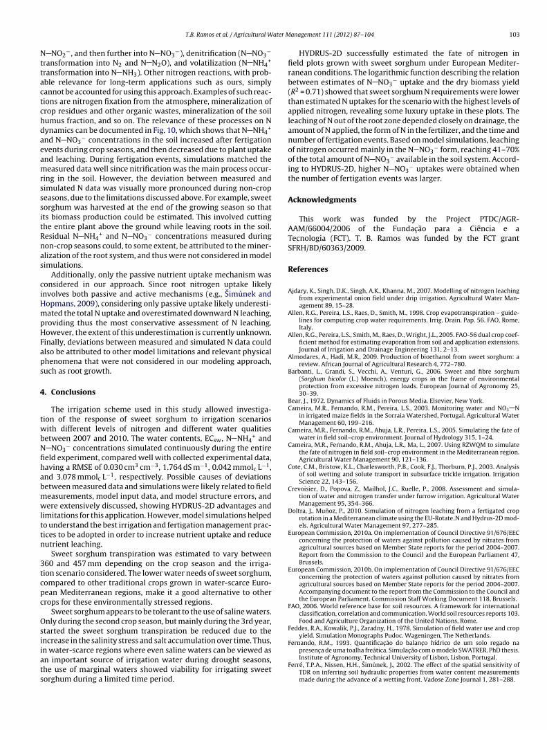
−
Fig. 13 shows the relationship between the N NO3 plantptake calculated using HYDRUS-2D and the experimentally deter-ined dry biomass yield expressed using a logarithmic functionith a R2 of 0.71. This logarithmic function fitted to experimentalig. 12. Simulated distributions of N NO3− concentration in plot I-A during crop season
he forth fertigation event (August 2, 2008), after the sixth and last fertigation event (AuguSeptember 30, 2008). The drip emitter was located in the top left corner of each contour
2, after sowing (May 15, 2008), after the first fertigation event (July 17, 2008), afterst 14, 2008), at the end of the irrigation period (September 9, 2008), and at harvest
plot.
data shows that an additional incremental increase of N NO3−
uptake produces diminishing returns in the total dry biomassresponse. Each additional unit of N NO3
− taken up by plant rootsadded less to the total biomass output than the previous unit did.After a certain level of N NO3
− uptake was reached (estimated hereto be between those registered for groups II-III, i.e., 130–180 kg/ha),further increases in nutrient uptake did not contribute directly tothe increase of the dry biomass yield. Group I thus involved some‘luxury’ uptake, since the amount of N NO3
− taken up by plant
roots did not contribute significantly to the dry biomass yield. Moredetailed results of the effect of brackish waters on nitrogen needsand dry biomass yield of sweet sorghum can be found in Ramoset al. (2012).2, after sowing (May 15, 2008), after the first fertigation event (July 17, 2008), afterst 14, 2008), at the end of the irrigation period (September 9, 2008), and at harvest
plot.
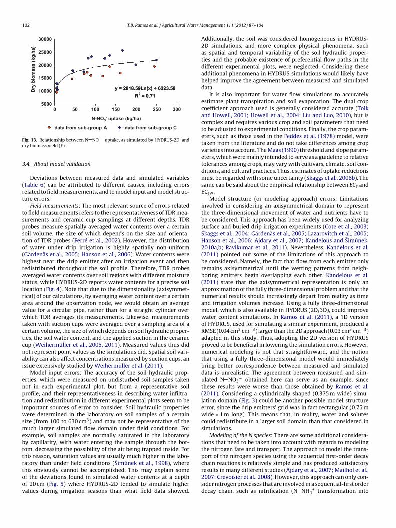
102 T.B. Ramos et al. / Agricultural Water M
y = 2818.59Ln(x) + 6223.58
R = 0.71
5000
10000
15000
20000
25000
30000
3002502001501000
N-NO3- (kg/ha)uptake
Dry
bio
ma
ss
(k
g/h
a)
y = 2818.59Ln(x) + 6223.58
R2 = 0.71
50
sub-group Cdata fromAsub-groupdata from
Fd
3
(rt
tspsto(hraslravwtctcnai
enptiwsmebttrtoov
ig. 13. Relationship between N NO3− uptake, as simulated by HYDRUS-2D, and
ry biomass yield (Y).
.4. About model validation
Deviations between measured data and simulated variablesTable 6) can be attributed to different causes, including errorselated to field measurements, and to model input and model struc-ure errors.
Field measurements: The most relevant source of errors relatedo field measurements refers to the representativeness of TDR mea-urements and ceramic cup samplings at different depths. TDRrobes measure spatially averaged water contents over a certainoil volume, the size of which depends on the size and orienta-ion of TDR probes (Ferré et al., 2002). However, the distributionf water under drip irrigation is highly spatially non-uniformGärdenäs et al., 2005; Hanson et al., 2006). Water contents wereighest near the drip emitter after an irrigation event and thenedistributed throughout the soil profile. Therefore, TDR probesveraged water contents over soil regions with different moisturetatus, while HYDRUS-2D reports water contents for a precise soilocation (Fig. 4). Note that due to the dimensionality (axisymmet-ical) of our calculations, by averaging water content over a certainrea around the observation node, we would obtain an averagealue for a circular pipe, rather than for a straight cylinder overhich TDR averages its measurements. Likewise, measurements
aken with suction cups were averaged over a sampling area of aertain volume, the size of which depends on soil hydraulic proper-ies, the soil water content, and the applied suction in the ceramicup (Weihermüller et al., 2005, 2011). Measured values thus didot represent point values as the simulations did. Spatial soil vari-bility can also affect concentrations measured by suction cups, anssue extensively studied by Weihermüller et al. (2011).
Model input errors: The accuracy of the soil hydraulic prop-rties, which were measured on undisturbed soil samples takenot in each experimental plot, but from a representative soilrofile, and their representativeness in describing water infiltra-ion and redistribution in different experimental plots seem to bemportant sources of error to consider. Soil hydraulic properties
ere determined in the laboratory on soil samples of a certainize (from 100 to 630 cm3) and may not be representative of theuch larger simulated flow domain under field conditions. For
xample, soil samples are normally saturated in the laboratoryy capillarity, with water entering the sample through the bot-om, decreasing the possibility of the air being trapped inside. Forhis reason, saturation values are usually much higher in the labo-atory than under field conditions (Simunek et al., 1998), where
his obviously cannot be accomplished. This may explain somef the deviations found in simulated water contents at a depthf 20 cm (Fig. 5) where HYDRUS-2D tended to simulate higheralues during irrigation seasons than what field data showed.anagement 111 (2012) 87– 104
Additionally, the soil was considered homogeneous in HYDRUS-2D simulations, and more complex physical phenomena, suchas spatial and temporal variability of the soil hydraulic proper-ties and the probable existence of preferential flow paths in thedifferent experimental plots, were neglected. Considering theseadditional phenomena in HYDRUS simulations would likely havehelped improve the agreement between measured and simulateddata.
It is also important for water flow simulations to accuratelyestimate plant transpiration and soil evaporation. The dual cropcoefficient approach used is generally considered accurate (Tolkand Howell, 2001; Howell et al., 2004; Liu and Luo, 2010), but iscomplex and requires various crop and soil parameters that needto be adjusted to experimental conditions. Finally, the crop param-eters, such as those used in the Feddes et al. (1978) model, weretaken from the literature and do not take differences among cropvarieties into account. The Maas (1990) threshold and slope param-eters, which were mainly intended to serve as a guideline to relativetolerances among crops, may vary with cultivars, climate, soil con-ditions, and cultural practices. Thus, estimates of uptake reductionsmust be regarded with some uncertainty (Skaggs et al., 2006b). Thesame can be said about the empirical relationship between ECe andECsw.
Model structure (or modeling approach) errors: Limitationsinvolved in considering an axisymmetrical domain to representthe three-dimensional movement of water and nutrients have tobe considered. This approach has been widely used for analyzingsurface and buried drip irrigation experiments (Cote et al., 2003;Skaggs et al., 2004; Gärdenäs et al., 2005; Lazarovitch et al., 2005;Hanson et al., 2006; Ajdary et al., 2007; Kandelous and Simunek,2010a,b; Ravikumar et al., 2011). Nevertheless, Kandelous et al.(2011) pointed out some of the limitations of this approach tobe considered. Namely, the fact that flow from each emitter onlyremains axisymmetrical until the wetting patterns from neigh-boring emitters begin overlapping each other. Kandelous et al.(2011) state that the axisymmetrical representation is only anapproximation of the fully three-dimensional problem and that thenumerical results should increasingly depart from reality as timeand irrigation volumes increase. Using a fully three-dimensionalmodel, which is also available in HYDRUS (2D/3D), could improvewater content simulations. In Ramos et al. (2011), a 1D versionof HYDRUS, used for simulating a similar experiment, produced aRMSE (0.04 cm3 cm−3) larger than the 2D approach (0.03 cm3 cm−3)adapted in this study. Thus, adopting the 2D version of HYDRUSproved to be beneficial in lowering the simulation errors. However,numerical modeling is not that straightforward, and the notionthat using a fully three-dimensional model would immediatelybring better correspondence between measured and simulateddata is unrealistic. The agreement between measured and sim-ulated N NO3
− obtained here can serve as an example, sincethese results were worse than those obtained by Ramos et al.(2011). Considering a cylindrically shaped (0.375 m wide) simu-lation domain (Fig. 3) could be another possible model structureerror, since the drip emitters’ grid was in fact rectangular (0.75 mwide × 1 m long). This means that, in reality, water and solutescould redistribute in a larger soil domain than that considered insimulations.
Modeling of the N species: There are some additional considera-tions that need to be taken into account with regards to modelingthe nitrogen fate and transport. The approach to model the trans-port of the nitrogen species using the sequential first-order decaychain reactions is relatively simple and has produced satisfactory
results in many different studies (Ajdary et al., 2007; Mailhol et al.,2007; Crevoisier et al., 2008). However, this approach can only con-sider nitrogen processes that are involved in a sequential-first orderdecay chain, such as nitrification (N NH4+ transformation into
ater M
NttactchdaeamrsssitRnas
ciHmpHFaps
4
twbNfihabmwlttn
3tcpc
Osiiats
T.B. Ramos et al. / Agricultural W
NO2−, and then further into N NO3
−), denitrification (N NO3−
ransformation into N2 and N N2O), and volatilization (N NH4+
ransformation into N NH3). Other nitrogen reactions, with prob-ble relevance for long-term applications such as ours, simplyannot be accounted for using this approach. Examples of such reac-ions are nitrogen fixation from the atmosphere, mineralization ofrop residues and other organic wastes, mineralization of the soilumus fraction, and so on. The relevance of these processes on Nynamics can be documented in Fig. 10, which shows that N NH4
+
nd N NO3− concentrations in the soil increased after fertigation
vents during crop seasons, and then decreased due to plant uptakend leaching. During fertigation events, simulations matched theeasured data well since nitrification was the main process occur-
ing in the soil. However, the deviation between measured andimulated N data was visually more pronounced during non-cropeasons, due to the limitations discussed above. For example, sweetorghum was harvested at the end of the growing season so thatts biomass production could be estimated. This involved cuttinghe entire plant above the ground while leaving roots in the soil.esidual N NH4
+ and N NO3− concentrations measured during
on-crop seasons could, to some extent, be attributed to the miner-lization of the root system, and thus were not considered in modelimulations.
Additionally, only the passive nutrient uptake mechanism wasonsidered in our approach. Since root nitrogen uptake likelynvolves both passive and active mechanisms (e.g., Simunek andopmans, 2009), considering only passive uptake likely underesti-ated the total N uptake and overestimated downward N leaching,
roviding thus the most conservative assessment of N leaching.owever, the extent of this underestimation is currently unknown.inally, deviations between measured and simulated N data couldlso be attributed to other model limitations and relevant physicalhenomena that were not considered in our modeling approach,uch as root growth.
. Conclusions
The irrigation scheme used in this study allowed investiga-ion of the response of sweet sorghum to irrigation scenariosith different levels of nitrogen and different water qualities
etween 2007 and 2010. The water contents, ECsw, N NH4+ and
NO3− concentrations simulated continuously during the entire
eld experiment, compared well with collected experimental data,aving a RMSE of 0.030 cm3 cm−3, 1.764 dS m−1, 0.042 mmolc L−1,nd 3.078 mmolc L−1, respectively. Possible causes of deviationsetween measured data and simulations were likely related to fieldeasurements, model input data, and model structure errors, andere extensively discussed, showing HYDRUS-2D advantages and
imitations for this application. However, model simulations helpedo understand the best irrigation and fertigation management prac-ices to be adopted in order to increase nutrient uptake and reduceutrient leaching.
Sweet sorghum transpiration was estimated to vary between60 and 457 mm depending on the crop season and the irriga-ion scenario considered. The lower water needs of sweet sorghum,ompared to other traditional crops grown in water-scarce Euro-ean Mediterranean regions, make it a good alternative to otherrops for these environmentally stressed regions.
Sweet sorghum appears to be tolerant to the use of saline waters.nly during the second crop season, but mainly during the 3rd year,
tarted the sweet sorghum transpiration be reduced due to thencrease in the salinity stress and salt accumulation over time. Thus,
n water-scarce regions where even saline waters can be viewed asn important source of irrigation water during drought seasons,he use of marginal waters showed viability for irrigating sweetorghum during a limited time period.anagement 111 (2012) 87– 104 103
HYDRUS-2D successfully estimated the fate of nitrogen infield plots grown with sweet sorghum under European Mediter-ranean conditions. The logarithmic function describing the relationbetween estimates of N NO3
− uptake and the dry biomass yield(R2 = 0.71) showed that sweet sorghum N requirements were lowerthan estimated N uptakes for the scenario with the highest levels ofapplied nitrogen, revealing some luxury uptake in these plots. Theleaching of N out of the root zone depended closely on drainage, theamount of N applied, the form of N in the fertilizer, and the time andnumber of fertigation events. Based on model simulations, leachingof nitrogen occurred mainly in the N NO3
− form, reaching 41–70%of the total amount of N NO3
− available in the soil system. Accord-ing to HYDRUS-2D, higher N NO3
− uptakes were obtained whenthe number of fertigation events was larger.
Acknowledgments
This work was funded by the Project PTDC/AGR-AAM/66004/2006 of the Fundac ão para a Ciência e aTecnologia (FCT). T. B. Ramos was funded by the FCT grantSFRH/BD/60363/2009.
References
Ajdary, K., Singh, D.K., Singh, A.K., Khanna, M., 2007. Modelling of nitrogen leachingfrom experimental onion field under drip irrigation. Agricultural Water Man-agement 89, 15–28.
Allen, R.G., Pereira, L.S., Raes, D., Smith, M., 1998. Crop evapotranspiration – guide-lines for computing crop water requirements. Irrig. Drain. Pap. 56. FAO, Rome,Italy.
Allen, R.G., Pereira, L.S., Smith, M., Raes, D., Wright, J.L., 2005. FAO-56 dual crop coef-ficient method for estimating evaporation from soil and application extensions.Journal of Irrigation and Drainage Engineering 131, 2–13.
Almodares, A., Hadi, M.R., 2009. Production of bioethanol from sweet sorghum: areview. African Journal of Agricultural Research 4, 772–780.
Barbanti, L., Grandi, S., Vecchi, A., Venturi, G., 2006. Sweet and fibre sorghum(Sorghum bicolor (L.) Moench), energy crops in the frame of environmentalprotection from excessive nitrogen loads. European Journal of Agronomy 25,30–39.
Bear, J., 1972. Dynamics of Fluids in Porous Media. Elsevier, New York.Cameira, M.R., Fernando, R.M., Pereira, L.S., 2003. Monitoring water and NO3 N
in irrigated maize fields in the Sorraia Watershed, Portugal. Agricultural WaterManagement 60, 199–216.
Cameira, M.R., Fernando, R.M., Ahuja, L.R., Pereira, L.S., 2005. Simulating the fate ofwater in field soil–crop environment. Journal of Hydrology 315, 1–24.
Cameira, M.R., Fernando, R.M., Ahuja, L.R., Ma, L., 2007. Using RZWQM to simulatethe fate of nitrogen in field soil–crop environment in the Mediterranean region.Agricultural Water Management 90, 121–136.
Cote, C.M., Bristow, K.L., Charlesworth, P.B., Cook, F.J., Thorburn, P.J., 2003. Analysisof soil wetting and solute transport in subsurface trickle irrigation. IrrigationScience 22, 143–156.
Crevoisier, D., Popova, Z., Mailhol, J.C., Ruelle, P., 2008. Assessment and simula-tion of water and nitrogen transfer under furrow irrigation. Agricultural WaterManagement 95, 354–366.
Doltra, J., Munoz, P., 2010. Simulation of nitrogen leaching from a fertigated croprotation in a Mediterranean climate using the EU-Rotate N and Hydrus-2D mod-els. Agricultural Water Management 97, 277–285.
European Commission, 2010a. On implementation of Council Directive 91/676/EECconcerning the protection of waters against pollution caused by nitrates fromagricultural sources based on Member State reports for the period 2004–2007.Report from the Commission to the Council and the European Parliament 47,Brussels.
European Commission, 2010b. On implementation of Council Directive 91/676/EECconcerning the protection of waters against pollution caused by nitrates fromagricultural sources based on Member State reports for the period 2004–2007.Accompanying document to the report from the Commission to the Council andthe European Parliament. Commission Staff Working Document 118, Brussels.
FAO, 2006. World reference base for soil resources. A framework for internationalclassification, correlation and communication. World soil resources reports 103.Food and Agriculture Organization of the United Nations, Rome.
Feddes, R.A., Kowalik, P.J., Zaradny, H., 1978. Simulation of field water use and cropyield. Simulation Monographs Pudoc. Wageningen, The Netherlands.
Fernando, R.M., 1993. Quantificac ão do balanc o hídrico de um solo regado na
presenc a de uma toalha freática. Simulac ão com o modelo SWATRER. PhD thesis.Institute of Agronomy, Technical University of Lisbon, Lisbon, Portugal.Ferré, T.P.A., Nissen, H.H., Simunek, J., 2002. The effect of the spatial sensitivity ofTDR on inferring soil hydraulic properties from water content measurementsmade during the advance of a wetting front. Vadose Zone Journal 1, 281–288.

1 ater M
F
G
G
G
H
H
H
H
H
J
K
K
K
K
K
L
L
M
M
M
M
M
M
M
M
N
P
04 T.B. Ramos et al. / Agricultural W
ontes, J.C., Pereira, L.S., Smith, R.E., 1992. Runoff and erosion in volcanic soils ofAzores: simulation with OPUS. Catena 56, 199–212.
ärdenäs, A., Hopmans, J.W., Hanson, B.R., Simunek, J., 2005. Two-dimensional mod-eling of nitrate leaching for various fertigation scenarios under micro-irrigation.Agricultural Water Management 74, 219–242.
onc alves, M.C., Leij, F.J., Schaap, M.G., 2001. Pedotransfer functions for solutetransport parameters of Portuguese soils. European Journal of Soil Science 52,563–574.
onc alves, M.C., Simunek, J., Ramos, T.B., Martins, J.C., Neves, M.J., Pires,F.P., 2006. Multicomponent solute transport in soil lysimeters withwaters of different quality. Water Resources Research 42, W08401,http://dx.doi.org/10.1029/2005WR004802.
anson, B.R., Simunek, J., Hopmans, J.W., 2006. Evaluation of urea-ammonium-nitrate fertigation with drip irrigation using numerical modeling. AgriculturalWater Management 86, 102–113.
anson, B.R., Simunek, J., Hopmans, J.W., 2008. Leaching with subsurface drip irri-gation under saline, shallow ground water conditions. Vadose Zone Journal 7,810–818.
offman, G.J., Shalhevet, J., 2007. Controlling salinity. In: Hoffman, G.J. (Ed.),Design and operation of farm irrigation systems. , 2nd ed. American Soci-ety of Agricultural and Biological Engineers, St. Joseph, Michigan, USA,pp. 160–207.
owell, T.A., Evett, R., Tolk, J.A., Schneider, A.D., 2004. Evapotranspiration of full-,deficit-irrigated, and dryland cotton on the Northern Texas High Plains. Journalof Irrigation and Drainage Engineering 130, 277–285.
utson, J.L., Wagenet, R.J., 1991. Simulating nitrogen dynamics in soils using a deter-ministic model. Soil Use and Management 7, 74–78.
ohnsson, H., Bergström, L., Jansson, P.-E., Paustian, K., 1987. Simulated nitrogendynamics and losses in a layered agricultural soil. Agriculture Ecosystems andEnvironment 18, 333–356.
andelous, M.M., Simunek, J., 2010a. Comparison of numerical, analytical andempirical models to estimate wetting pattern for surface and subsurface dripirrigation. Irrigation Science 28, 435–444.
andelous, M.M., Simunek, J., 2010b. Numerical simulations of water movement ina subsurface drip irrigation system under field and laboratory conditions usingHYDRUS-2D. Agricultural Water Management 97, 1070–1076.
andelous, M.M., Simunek, J., van Genuchten, M.Th., Malek, K., 2011. Soil water con-tent distributions between two emitters of a subsurface drip irrigation system.Soil Science Society of America Journal 75, 488–497.
aterji, N., Mastrorilli, M., Rana, G., 2008. Water use efficiency of crops cultivated inthe Mediterranean region: review and analysis. European Journal of Agronomy28, 493–507.
lepper, B., 1991. Crop root system response to irrigation. Irrigation Science 12,105–108.
azarovitch, N., Simunek, J., Shani, U., 2005. System-dependent boundary conditionfor water flow from subsurface source. Soil Science Society of America Journal69, 46–50.
iu, Y.J., Luo, Y., 2010. A consolidated evaluation of the FAO-56 dual crop coefficientapproach using the lysimeter data in the North China Plain. Agricultural WaterManagement 97, 31–40.
a, L., Ahuja, L.R., Ascough II, J.C., Shaffer, M.J., Rojas, K.W., Malone, R.W., Cameira,M.R., 2001. Integrating system modeling with field research in agriculture: appli-cations of the root zone water quality model (RZWQM). Advances in Agronomy71, 233–292.
ailhol, J.C., Crevoisier, D., Triki, K., 2007. Impact of water application conditionson nitrogen leaching under furrow irrigation: experimental and modellingapproaches. Agricultural Water Management 87, 275–284.
ailhol, J.C., Ruelle, P., Walser, S., Schütze, N., Dejean, C., 2011. Analysis of AETand yield predictions under surface and buried drip irrigation systems usingthe Crop Model PILOTE and Hydrus-2D. Agricultural Water Management 98,1033–1044.
allants, D., van Genuchten, M.Th., Simunek, J., Jacques, D., Seetharam, S., 2011.Leaching of contaminants to groundwater. In: Swartjes, F.A. (Ed.), Dealingwith Contaminated Sites. From Theory to Practical Applications. Springer, TheNetherlands, pp. 787–850.
aas, E.V., 1990. Crop salt tolerance. In: Tanji, K.K. (Ed.), Agricultural Salinity Assess-ment and Management. Manual on Engineering Practice, vol. 71. AmericanSociety of Civil Engineers, Reston, VA, pp. 262–304.
astrorilli, M., Katerji, N., Rana, G., Steduto, P., 1995. Sweet sorghum in Mediter-ranean climate: radiation use and biomass water use efficiencies. Industrial Cropand Products 3, 253–260.
astrorilli, M., Katerji, N., Rana, G., 1999. Productivity and water use efficiency ofsweet sorghum as affected by soil water deficit occurring at different vegetativegrowth stages. European Journal of Agronomy 11, 207–215.
molawa, K., Or, D., 2003. Experimental and numerical evaluation of analytical vol-ume balance model for soil water dynamics under drip irrigation. Soil Science
Society of America Journal 67, 1657–1671.ovák, V., van Genuchten, M.Th., 2008. Using the transpiration regime to estimatebiomass production. Soil Science 173, 401–407.
ereira, L.S., van den Broek, B., Kabat, P., Allen, R.G., 1995. Crop–Water SimulationModels in Practice. Wageningen Pers, Wageningen, The Netherlands.
anagement 111 (2012) 87– 104
Prasad, S., Singh, A., Jain, N., Joshi, H.C., 2007. Ethanol production from sweetsorghum syrup for utilization as automotive fuel in India. Energy and Fuel 21,2415–2420.
Ramos, T.B., Gonc alves, M.C., Castanheira, N.L., Martins, J.C., Santos, F.L., Prazeres, A.,Fernandes, M.L., 2009. Effect of sodium and nitrogen on yield function of irri-gated maize in southern Portugal. Agricultural Water Management 96, 585–594.
Ramos, T.B., Simunek, J., Gonc alves, M.C., Martins, J.C., Prazeres, A., Castanheira,N.L., Pereira, L.S., 2011. Field evaluation of a multicomponent solute transportmodel in soils irrigated with saline waters. Journal of Hydrology 407, 129–144,http://dx.doi.org/10.1016/j.jhydrol.2011.07.016.
Ramos, T.B., Castanheira, N.L., Gonc alves, M.C., Fernandes, M.L., Januário, M.I.,Lourenc o, M.E., Pires, F.P., Martins, J.C., 2012. Effect of combined use of brack-ish water and nitrogen fertilizer on biomass and sugar yield of sweet sorghum.Pedosphere, in press.
Ravikumar, V., Vijayakumar, G., Simunek, J., Chellamuthu, S., Santhi, R., Appavu, K.,2011. Evaluation of fertigation scheduling for sugarcane using a vadose zoneflow and transport model. Agricultural Water Management 98, 1431–1440.
Ritchie, J.T., 1972. Model for predicting evaporation from a row crop with incompletecover. Water Resources Research 8, 1204–1213.
Roberts, T., Lazarovitch, N., Warrick, A.W., Thompson, T.L., 2009. Modeling salt accu-mulation with subsurface drip irrigation using HYDRUS-2D. Soil Science Societyof America Journal 73, 233–240.
Roberts, T., White, S.A., Warrick, A.W., Thompson, T.L., 2008. Tape depth and ger-mination method influence patterns of salt accumulation with subsurface dripirrigation. Agricultural Water Management 95, 669–677.
Rosa, R.D., Paredes, P., Rodrigues, G.C., Alves, I., Fernando, R.M., Pereira, L.S., Allen,R.G., 2012. Implementing the dual crop coefficient approach in interactivesoftware: 1. Background and computational strategy. Agricultural Water Man-agement 103, 62–77.
Simunek, J., Wang, D., Shouse, P.J., van Genuchten, Th.M., 1998. Analysis of a fieldtension disc infiltrometer experiment by parameter estimation. InternationalAgrophysics 12, 167–180.
Simunek, J., van Genuchten, Th.M., Sejna, M., 2006. The HYDRUS software packagefor simulating two- and three-dimensional movement of water, heat, and mul-tiple solutes in variably-saturated media. In: Technical Manual. Version 1.0. PCProgress, Prague, Czech Republic, 241 p.
Simunek, J., van Genuchten, M.Th., Sejna, M., 2008. Development and applications ofthe HYDRUS and STANMOD software packages, and related codes. Vadose ZoneJournal 7, 587–600.
Simunek, J., Hopmans, J.W., 2009. Modeling compensated root water and nutrientuptake. Ecological Modelling 220, 505–521.
Skaggs, T.H., Trout, T.J., Simunek, J., Shouse, P.J., 2004. Comparison of HYDRUS-2Dsimulations of drip irrigation with experimental observations. Journal of Irriga-tion and Drainage Engineering 130, 304–310.
Skaggs, T.H., van Genuchten M.Th. Shouse, P.J., Poss, J.A., 2006a. Macroscopicapproaches to root water uptake as a function of water and salinity stress.Agricultural Water Management 86, 140–149.
Skaggs, T.H., Shouse, P.J., Poss, J.A., 2006b. Irrigating forage crops with saline waters:2. Modeling root uptake and drainage. Vadose Zone Journal 5, 824–837.
Steduto, P., Katerji, N., Puertos-Molina, H., Unlü, M., Mastrorilli, M., Rana, G., 1997.Water-use efficiency of sweet sorghum under water stress conditions. Gas-exchange investigations at leaf and canopy scales. Field Crops Research 54,221–234.
Tolk, J.A., Howell, T.A., 2001. Measured and simulated evapotranspiration of grainsorghum grown with full and limited irrigation in three High Plains soils. Trans-actions of ASABE 44, 1553–1558.
U.S. Salinity Laboratory Staff, 1954. Diagnosis and Improvement of Saline and AlcalySoils. USDA Handbook 60. Washington, USA.
van Genuchten, M.Th., 1980. A closed form equation for predicting the hydraulicconductivity of unsaturated soils. Soil Science Society of America Journal 44,892–898.
van Genuchten, M.Th., 1987. A numerical model for water and solute movementin and below the root zone. Res. Rep. 121, U.S. Salinity Laboratory, USDA, ARS,Riverside, California.
Vasilakoglou, I., Dhima, K., Karagiannidis, N., Gatsis, T., 2011. Sweet sorghum pro-ductivity for biofuels under increased soil salinity and reduced irrigation. FieldCrops Research 120, 38–46.
Vrugt, J.A., Hopmans, J.W., Simunek, J., 2001. Calibration of a two dimensional rootwater uptake model. Soil Science Society of America Journal 65, 1027–1037.
Weihermüller, L., Kasteel, R., Vanderborght, J., Pütz, T., Vereecken, H., 2005. Soilwater extraction with a suction cup: results of numerical simulations. VadoseZone Journal 4, 899–907.
Weihermüller, L., Kasteel, R., Vanderborght, J., Simunek, J., Vereecken, H., 2011.Uncertainty in pesticide monitoring using suction cups: evidence from numer-ical simulations. Vadose Zone Journal 10, 1287–1298.
Zegada-Lizarazu, W., Zatta, A., Monti, A., 2012. Water uptake efficiency and above-
and belowground biomass development of sweet sorghum and maize underdifferent water regimes. Plant Soil 351, 47–60.Zhao, Y.L., Dolat, A., Steinberger, Y., Wang, X., Osman, A., Xie, G.H., 2009. Biomassyield and changes in chemical composition of sweet sorghum cultivars grownfor biofuel. Field Crops Research 111, 55–64.