Embed Size (px)
Citation preview
AIAA 2002–1408
OPTIMIZATION OF PERFECT AND IMPERFECT RING AND STRINGERSTIFFENED CYLINDRICAL SHELLS WITH PANDA2 AND EVALUATION
OF THE OPTIMUM DESIGNS WITH STAGS
David Bushnell,* Fellow, AIAA, RetiredCharles Rankin, Associate Fellow, AIAA
Lockheed Martin Advanced Technology CenterDept. L9-21, Bldg. 204, 3251 Hanover St., Palo Alto, CA 94304
* Copyright 2002 by David Bushnell. Publishedby the American Institute of Aeronautics andAstronautics, Inc, with permission
ABSTRACT
Ring and stringer stiffened perfect and imperfect an-gle-ply cylindrical shells under combined axial com-pression and in-plane shear are optimized with a pro-gram called PANDA2 for the minimum weight de-sign of stiffened panels, and the optimum designs arethen evaluated with use of a general purpose finiteelement code called STAGS. The good agreementbetween PANDA2 and STAGS predictions for thenonlinear collapse of imperfect stiffened shells justi-fies the use of PANDA2 for preliminary design. Anew PANDA2 processor called STAGSUNIT auto-matically generates STAGS input files for cylindricalpanels and shells with both stringers and rings thathave various open cross sections such as Blades,Zees, Jays, Tees and Is. In STAGSUNIT the edgeconditions are formulated so that STAGS models ofsubdomains of a long cylindrical shell with manystiffeners can be constructed that do not have artifi-cial prebuckling stress concentrations near the edgesthat might significantly affect predictions of bifurca-tion buckling and nonlinear collapse of the subdo-main. Many STAGS models of optimized shells andsubdomains of shells with Blade, Zee, and Tee stiff-ening are generated and explored, both with respectto linear bifurcation buckling and nonlinear collapse.The behavior of shells with an initial imperfection inthe form of a general buckling mode of the imperfectshell is described from a physical point of view.Some difficulties encountered during this project aredescribed.
INTRODUCTION
Purpose of this paper
The main purpose of this paper is to present mini-mum-weight designs derived by PANDA2 [1-10] forcertain perfect and imperfect composite ring and
stringer-stiffened cylindrical shells and to comparethese with predictions from STAGS [11-13] for theoptimized structures. PANDA2 and STAGS are de-scribed. A new PANDA2 processor called STA G-SUNIT is described. STAGSUNIT automatically gen-erates STAGS input files for ring and stringer stiff-ened panels and shells optimized by PANDA2. A l-though the development and analysis of optimum de-signs for which one or more of the design load comb i-nations exceeds the local buckling load of the panelskin are within the scopes of both PANDA2 andSTAGS, in this paper the stiffened shells are opti-mized such that local postbuckling deformation of theskin is not allowed in the PANDA2 models.
Brief review of the literature
Local and overall bifurcation buckling of stiffenedpanels can be determined with the BUCLASP code[14] and with the newer successors to BUCLASP andVIPASA: the PANDA2 [1-10], POSTOP [15], VI-CONOPT [16], and PASCO [17] codes. PASCO, VI-CONOPT, PANDA2 and POSTOP are capable of ob-taining optimum designs of such panels, andPANDA2, POSTOP and VICONOPT can do so in-cluding the effect of local postbuckling [3] of thepanel skin and/or parts of the stringers. One of thePANDA2 processors, called STAGSMODEL [4]automatically sets up a finite element model of a panelpreviously optimized with PANDA2. The [PANDA2,STAGSMODEL, STAGS] combination has been usedmany times to optimize and evaluate optimum designsof panels under combined loads for service in thepostbuckling regime [3,4,8]. Other works are brieflysurveyed in Ref.[16] cited in [8].
2American Institute of Aeronautics and Astronautics
DESCRIPTION OF PANDA2
PANDA2 is a computer program for the minimumweight design of stiffened, composite, flat or cylin-drical, perfect or imperfect panels and shells sub-jected to multiple sets of combined in-plane loads,normal pressure, edge moments, and temperature.For most configurations the panels can be locallypostbuckled [3]. Previous work on PANDA2 isdocumented in [1-10]. PANDA2 incorporates thetheories of earlier codes PANDA [2] and BOSOR4[18]. The optimizer used in PANDA2 is called ADS[19]. Panels are optimized subject primarily to buck-ling and stress constraints.
PANDA2 processors and types of analysis
As described in [1-10], the PANDA2 system consistsof several processors, BEGIN, SETUP, DECIDE,MAINSETUP, PANDAOPT, CHOOSEPLOT,CHANGE, STAGSMODEL, STAGSUNIT, etc. Thefunctions of these processors are as follows:
BEGIN User establishes starting design, materialproperties, prebuckling and buckling boundary con-ditions.
SETUP System sets up BOSOR4-type templates forstiffness and load-geometric matrices.
DECIDE User chooses decision variables andbounds and sets up equality and inequality con-straints.
MAINSETUP User chooses analysis type, loading,and solution strategies.
PANDAOPT Analysis type is performed (e.g. opti-mization).
CHOOSEPLOT User chooses what to plot.
DIPLOT The system obtains plots (postscript files).
CHANGE User changes selected variables and con-stants.
AUTOCHANGE A new starting design is automati-cally generated in a random manner.
SUPEROPT An attempt is made to find a global op-timum design.
PANEL A BOSOR4 input file is generated for inter-ring buckling of panel skin and stringers, with string-ers modelled as flexible shell branches.
PANEL2 A BOSOR4 input file is generated for inter-ring buckling of panel skin+smeared stringers withrings modelled as flexible shell branches.
STAGSMODEL An input file for STAGS [4,11-13]is generated (one finite element unit, only stringers arepermitted).
STAGSUNIT An input file for STAGS is generated(multiple shell units, both stringers and rings are per-mitted).
CLEANPAN Delete all files except files containinguser-provided input data for BEGIN, DECIDE,MAINSETUP, CHANGE, PANEL, PANEL2,STAGSMODEL and STAGSUNIT.
PANDA2 can be run in five modes:
1. Optimization2. simple analysis of a fixed design3. test simulation4. design sensitivity5. load-interaction (Nx,Ny), (Nx,Nxy), (Ny,Nxy)
Types of buckling included in PANDA2
PANDA2 computes general, inter-ring, and local skinbuckling loads and mode shapes. General buckling isbuckling in which both stringers (or isogrid stiffeners)and rings participate; “panel” (inter-ring) buckling isbuckling between adjacent rings in which stringers (orisogrid stiffeners) participate but the lines of intersec-tion of ring web roots with the panel skin do nottranslate; local buckling is buckling of the panel skinbetween adjacent stringers (or isogrid stiffeners) andrings. PANDA2 includes the following buckling mo d-els:
1. A discretized single skin-stringer module of thetype shown in Fig.1 of [9], for example. Thismodel is used for local buckling, local postbuck-ling, and wide column buckling of the panel re-gion between adjacent rings (transverse stiffen-ers).
2. Simple models for the buckling of the panel skinand stiffener segments of the type described in[2]. Typical buckling modes of the panel skin andstiffeners are shown in Fig. 6 of [2]. In the panelskin the buckling nodal lines are assumed to bestraight, as shown in Fig. 9 of [2]. This type ofbuckling model is used in some of the softwarewritten by Arbocz and Hol [20-22] and by Khotand his colleagues [23,24]. These models are
3American Institute of Aeronautics and Astronautics
called "PANDA-type (closed form)" inPANDA2 jargon because they are the only onesused in the original PANDA program [2], whichwas superseded by PANDA2 [1] many yearsago. Over the years an elaborate strategy hasbeen developed in order to ensure that for eachtype of buckling in this “PANDA-type” cate-gory, the most critical (lowest) buckling loadfactor is not missed. The critical eigenvalue isdetermined from several searches over variousregions in the (m,n,slope) domain, where m is thenumber of axial halfwaves, n is the number ofcircumferential halfwaves, and “slope” is theslope of the buckling nodal lines (non-zero whenthere is in-plane shear loading and/or shell wallanisotropy). More details are given in [10].
For sandwich panels and shells PANDA2 com-putes load factors for additional types of buck-ling that only occur for sandwich walls: facesheet wrinkling, buckling over the diameter of asingle cell of a honeycomb core, and corecrimping [7].
Three additional buckling models were recentlyadded to PANDA2 as described in [9]:
3. Local buckling between adjacent stringers andrings of a cylindrical or flat panel obtained froma Ritz model in which the buckling modal dis-placement components, u, v, w, are expanded indouble trigonometric series. The local region isassumed to be simply supported on all fouredges.
4. General buckling of a cylindrical panel in whichstringers and rings are treated as discrete beamswith undeformable cross sections. Again, thegeneral buckling modal displacement comp o-nents, u, v, w, are expanded in double trigono-metric series. The edges of the domain are as-sumed to be simply supported and to have dis-crete stiffeners of half the user-specifiedmodulus. The domain for this model is a three-bay by three-bay subdomain of the entire panel.
5. A discretized single module model for a cylin-drical panel in which the ring segments andpanel skin-with-smeared-stringers are discretizedas shown in Fig. 30 of [9]. Until the work lead-ing to [9] was competed, the only discretizedmodule model in PANDA2 involved the panelskin and STRINGER segments. The RINGSwere "second-class citizens". In the discretizedskin-with-smeared-stringers/ring "branchedshell" model the cross sections of the rings can
deform in the buckling mode, since they are sub-divided into finite elements of the type used inBOSOR4 [18].
Buckling loads corresponding to a given type of buck-ling (such as local buckling of the skin between string-ers or general buckling) may be computed by morethan one model in order to verify results and to pro-vide appropriate knockdown factors to account foranisotropy, inherent unconservativeness in smearingstiffeners, the presence of in- plane shear loading, andvariation of in-plane loading within the domain thatbuckles. The effect of transverse shear deformation isaccounted for as described in [1].
PANDA2 can optimize imperfect stiffened panels andshells [5]. The effects of initial geometric imperfec-tions are described below.
Local post buckling analysis
An analysis branch exists in which local post bucklingof the panel skin is accounted for [3,25]. In this brancha constraint condition that prevents stiffener pop-off isintroduced into the optimization calculations [1]. Thepostbuckling theory incorporated into PANDA2 issimilar to that formulated by Koiter for panels loadedinto the far postbuckling regime [25].
Stress constraints
In addition to buckling constraints, PANDA2 com-putes stress constraints including local postbucklingdeformations and thermal loading by both curing andapplied temperature distributions. For laminated com-posite walls PANDA2 generates stress constraintscorresponding to maximum tension along fibers,maximum compression along fibers, maximum ten-sion transverse to fibers, maximum compressiontransverse to fibers, and maximum in-plane shearstress for each different material in a stiffened panel.For isotropic material PANDA2 generates stress con-straints based on the von Mises effective stress.
Global optimizer SUPEROPT
Global optimum designs can be obtained withPANDA2 by means of a processor called “SUPER-OPT”, which is described in more detail in [6]. Atintervals during the optimization process new “start-ing” designs are automatically generated as follows:
DNiidxixiy ,..,2,1 )],(1)[()( =+= (1)
4American Institute of Aeronautics and Astronautics
where ND is the number of decision variables, x(i) isthe old value of the ith decision variable, y(i) is thenew value, and dx(i) is a random number between -0.5 and +1.5 if the decision variable is other than astiffener spacing and a random number between -1.0and +1.0 if the decision variable is a stiffener spac-ing. The difference in treatment for decision variablesthat are not stiffener spacings from those that arestiffener spacings results from early experiments withSUPEROPT [6].
BRIEF DESCRIPTION OF STAGS
STAGS (Structural Analysis of General Shells), is ashell finite element program with a strong bias to-wards stability analysis capabilities [11-13]. Apartfrom having a good nonlinear shell modeling capa-bility (small strain but arbitrarily large displacementsand rotations), STAGS is also equipped with path-following techniques that make it possible to solvestability problems such as bifurcation buckling andcollapse. The modeling capabilities include manydesign features that are frequently encountered inlightweight structures in the field of aero- and astro-nautics: a whole range of stiffener models, shell wallmaterials including composites, etc. In addition to thesolution techniques for computing the static equilib -rium branches of these models, STAGS also pos-sesses robust transient time stepping methods.
PANDA2 PROCESSOR “STA GSUNIT”
Introduction
Most of the effort expended to produce this paper ledto the creation of a new PANDA2 processor calledSTAGSUNIT. STAGSUNIT uses the PANDA2 da-tabase plus some interactive input from the user toproduce the two input files for STAGS called *.binand *.inp, in which "*" signifies the user-selectedname for the case.
Table 1 lists typical input data for the new processor,STAGSUNIT. In this particular case the user is ask-ing for an INDIC = 1 type of STAGS analysis (linearbifurcation buckling). Execution of STAGSUNITproduces the two STAGS input files, *.inp and *.bin.Table 2 lists the first part of the STAGS input file,*.inp in the annotated format automatically producedby STAGSUNIT. Table 3 lists the annotated *.binfile. Execution of STAGS followed by the STAGSpostprocessor called STAPL produces plots of thetype shown in Figs. 1 - 3. The STAGS input file,*.inp, is quite long. Table 4 lists just the headings inthe *.inp file corresponding to Fig. 1, in which the
cylindrical panel and all stiffener segments are mo d-eled as shell units with 480 finite elements.
Scope of STAGSUNIT
STAGSUNIT works for cylindrical panels stiffened bystringers and/or rings with blade, T, I, J, or Z crosssections. Unstiffened panels can also be processed.The cylindrical panel can span less than 360 degreesof circumference, as shown in Figs. 1 - 3, or can forma complete (360-deg) closed cylindrical shell. Thepanel skin and various stiffener parts are modeled as(what is called in STAGS jargon) "shell units". All orparts of the stiffeners can be modeled as discrete beamelements (210 finite elements) or as shell units. Theuser has five choices with regard to each set of stiffen-ers, stringers and rings. For stringers, for example, thechoices are identified in the PANDA2 PROMPT.DATfile [10] as follows:
Stringer modeling index must be 1 or 2 or 3 or 4 or5:
1 = all stringer segments are modeled as beams (210elements) that are attached to the cylindrical shell.
2 = stringer webs are modeled as shell branches (410elements) and any faying and/or outstanding flangesare modeled as beams (210 elements). The fayingflanges are attached to the cylindrical shell and theoutstanding flanges are attached at the tips of thestringer webs.
3 = all stringer segments (faying flange, web, out-standing flange) are modeled as shell branches.
4 = the stringer faying flange is modeled as a beam(210 elements), but the stringer web and stringeroutstanding flange are modeled as shell branches.
5 = the stringers are replaced by enforcement of aconstraint that the normal displacement w be con-stant along the generator where the stringer would beattached to the cylindrical shell. (NOTE: the correctprebuckling loading of the panel skin is used, that is,the actual stringers absorb their share of theprebuckling axial load.)
The same choices are provided in the modeling ofrings.
Edge conditions
A large part of the effort of creating a reliable STA G-SUNIT processor was spent on formulating properedge conditions so that:
5American Institute of Aeronautics and Astronautics
1. failure (bifurcation buckling and nonlinear col-lapse) as predicted from the STAGS modelwould probably not be in an "edge" mode in-duced by artificially introduced stress concentra-tions there, and
2. near-uniformity of the prebuckled stress statewould be assured. (NOTE: the axisymmetricprebuckling "hungry horse" deformation causedby the rings [5] will still occur.)
In other words, failure would not be caused by one ormore localized stress concentrations in the neighbor-hoods of one or more of the panel edges. The advan-tages of this favorable characteristic are:
1. The prebuckled state better simulates the modelon which PANDA2 predictions are based, and
2. One can obtain similar results for subdomains ofvarious sizes extracted from the full-sized panelor shell analyzed via PANDA2. There is amaximum numerical size of a STAGS modelthat can practically be processed. Therefore, onemust often obtain predictions of failure fromSTAGS models that are based on a subdomain ofthe actual shell rather than on the entire shell.
Table 5 lists the part of the *.inp file (abridged tosave space) concerned with edge conditions forSTAGS models of the type shown in Figs. 1 - 3. Thepartial compatibility (g-2) record, "v=const", that is,constant circumferential displacement v along thecurved panel edge at row 1 (x=0), permits uniform in-plane shear loading (torque) to be applied along row1. The four "w=const" constraints along the fouredges of the cylindrical panel eliminate any Poisson-ratio-induced nonuniformity in the prebuckling nor-mal displacement field (w ) in the neighborhoods ofthese edges. The contraints "ru=const" (no rotationabout the generators) along row 1 (x=0) and row 41(x=L) prevent numerical instability sometimes exp e-rienced in nonlinear STAGS runs when these con-straints are omitted. The "w=constant" records for thestringer and ring faying and outstanding flanges helpto prevent stiffener sidesway at the panel edges. Thetwo sets of Lagrange constraints to prevent stringerand ring sidesway (only headings listed here to savespace) force the webs of the stringers and rings toremain oriented radially at the edges of the panel.Even if stiffener sidesway is prevented, the out-standing flange is permitted to rotate in its plane, ascan be seen at the ends of the stringers shown in Fig.3. The four sets of Lagrange constraints to imposelinear variation of axial displacement u and circum-ferential displacement v along the two straight edges
permit uniform axial compression and in-plane shearloading along these two edges while generally pre-venting incremental buckling modal u and v comp o-nents. The last five sets of Lagrange constraints are notpresent, of course, if the STAGS model is a closed(360-deg.) cylindrical shell.
Except in rare cases such as that shown in Fig. 4, thesedisplacement constraints have the effect of causing theincremental bifurcation buckling modal displacementcomponents u, v, and w to be zero along the paneledges where the constraints are applied. An exceptionis displayed in Fig. 4. The lowest buckling load for theaxially compressed blade-stiffened cylindrical shellshown in Fig. 4 has a mode shape with the maximumnormal modal displacement w at the boundary x = L.In this mode w is constant along the circumference at x= L. This “spurious” mode is avoided, as will be seenlater, through the use of 480 finite elements with asparser nodal point mesh near the boundary than in theinterior of the shell. The mode is also avoided if, inhis/her input to the STAGSUNIT processor, the userspecifies that rings be located at the ends of the shell.
Along the curved edge at x = L = XSTAGS the cir-cumferential displacement v is fixed at zero. (See thesecond-to-last line of Table 5: "101 111" means all sixdisplacement and rotation components are free exceptthe circumferential displacement component v, whichis held at zero both in the prebuckling and bifurcationbuckling phases of the analysis.
Drilling freedoms suppressed
Table 4 lists many headings in the *.inp file containingthe phrase, “drilling freedoms suppressed..” When the480 finite element is used in a STAGS model, espe-cially one involving nonlinear analysis, it is necessaryto suppress the "sixth" nodal point degree of freedom:rotation about a normal to the shell. This "drilling"freedom should be suppressed everywhere except atnodal points where shell units intersect at some non-zero angle. Hence, when the user specifies use of the480 finite element, drilling freedoms are suppressed inSTAGS models generated via STAGSUNIT every-where except where stiffener segments intersect eachother or where they intersect the cylindrical skin at anangle other than zero. In a case with drilling freedomsnot suppressed, the nonlinear STAGS analysis failedto converge for a load factor PA in excess of 0.137With the same model with drilling freedoms appropri-ately suppressed, a converged stable equilibrium statewas obtained by STAGS for a maximum load factor ofabout 0.95. (This example involved an axially com-pressed optimized perfect blade stiffened cylindricalshell with a very, very small "triggering" initial imper-
6American Institute of Aeronautics and Astronautics
fection. PANDA2 predicted bifurcation buckling at aload factor of 1.0 and STAGS predicted linear bifur-cation buckling at a load factor of 0.978. (SeeFig.20.)
Various material, beam, and wall types
Almost half of the headings listed in Table 4 are con-cerned with the STAGS input libraries for materialtypes (ITAM), beam cross section types (ITAB), andshell wall types (ITAW). These three libraries havetwo sections, one concerned with types not at an edgeand the other concerned with types at an edge of thepanel. In STAGSUNIT, stiffeners that run alongedges are assigned materials with half the moduli anddensities of the corresponding members that are notlocated at an edge. Because of this construction thebehavior of a subdomain of the panel is permitted tobehave in a manner similar to that of the entire panel.
For each stiffener there are three segments: the fayingflange, the web, and the outstanding flange. Each ofthese segments is considered to be a separate discretebeam (210 elements used) and/or shell unit (410, 411,or 480 elements). Note: Only 410 shell elements canbe used in the STAGS model if there exist in thesame model discrete beams attached to the shell or tostiffener webs that are mo deled as shell units.
Fasteners
In STAGS fasteners are like little springs that con-nect nodes across gaps in the finite element model. Itis sometimes necessary to use fasteners in theSTAGS models produced by STAGSUNIT becausein optimum designs obtained by PANDA2 (espe-cially for the cases that are the subject of this study),the heights of the stiffener webs are sometimes of thesame magnitude as the thicknesses of the panel skinand faying flanges. Figures 2a,b show a STAGSmodel produced by STAGSUNIT in which fastenersare used. It can be seen, especially in Fig. 2b, that thegap between the stringers and the panel skin shouldnot be neglected. This gap represents the thickness ofthe faying flange plus half of the thickness of thecylindrical skin. (The reference surface of the cylin-drical skin is its middle surface in this case. See Fig.5b.) In PANDA2 models the roots of the stiffenerwebs are assumed to be attached to the outer surfaceof the faying flange, as shown in Fig. 5a (except withZ-stiffeners, for which the web line of attachment isat the middle surface of the faying flange). Theheight H of the web is the distance from the root ofthe web to the middle surface of the outstandingflange. In the STAGS model shown in Fig. 2b, theshort segments that represent the reference surfaces
of the faying flanges of the stringers are located at theouter surfaces of these faying flanges (Fig. 5b).
If the user elects in STAGSUNIT not to include fas-teners (see the appropriate entry near the bottom ofTable 1), the outstanding flanges of the stringers andthe web tips would have the identical locations ofthose shown in Fig. 2b, but the web would be ex-tended radially inward to the reference surface of thecylindrical shell, as illustrated in Figs. 5c and 6. Insuch a case the user would select the outer surface ofthe cylindrical shell as the reference surface (providedthe stringers are external). For external stiffenersSTAGSUNIT would automatically select the innersurface of each faying flange as its reference surface,as shown in Fig. 6. This is done in order that all shellunits are properly joined in the STAGS model, that is,there are no gaps where shell units are joined. STAGSdoes not permit gaps between shell units unless thesegaps are "bridged" by fasteners, rigid links, or mounts.
Figures 5 and 6 display examples of fabrications andtheir STAGS models. Fig. 5b shows the STAGSmodel when the stiffener is attached to the panel skinwith a fastener (actually, a "vector" of fasteners alongthe web root). Fig. 5c is the STAGS model when thereare no fasteners, and Fig. 6 is the case where there arerings and stringers on opposite sides of the shell andno fasteners.
In the STAGS input file *.inp a library of fastenerproperties is included with the other libraries of mate-rials, beam cross section properties, and shell unit wallproperties. The fasteners themselves are entered asfinite element units following data for all of the shellunits. The PANDA2 processor STAGSUNIT alwayssupplies just one entry in the library of fasteners: aspring with stiffness equal to six times the average ofthe axial and hoop stiffnesses of the panel skin. Thatis, the fastener spring constant equals ( )22113 CC + .
Because of this relatively stiff spring the fastener actsin a manner similar to a rigid link. Rigid links weretried but were found to be unworkable in the presentstudy because of conflict with certain of the edge andanti-sidesway conditions discussed in a previous sub-section. Rigid links generate Lagrange constraints,some of which involve the same nodal points as theedge conditions. This duplication of Lagrange con-straints generates ill conditioned equation systems.Fasteners do not generate any constraint conditions;they are simply additional parts of the structure andcontribute to its strain energy. The numerical size ofthe STAGS model is much smaller when fasteners areused than when rigid links are introduced.
7American Institute of Aeronautics and Astronautics
Choice of shell element (410 or 480)
In the writer's opinion (Bushnell) the most reliablefinite element in the STAGS element library is the480 [26] because buckling load factors from modelsconstructed with this element almost always con-verge from above the "exact" value. Hence, it is al-most always safe for the user to specify a low-densitynodal point mesh in areas where he/she is not inter-ested in obtaining local buckling behavior, such asnear the panel edges in the cases studied here. Localbuckling will occur first in areas of high nodal pointdensity.
With use of the 410 element [27] this is not alwaystrue. Figure 7 shows an optimized, stiffened cylindri-cal shell. Nodal points are concentrated near themidlength of the shell. However for the applied loadsystem (axial load Nx = -100 lb/in and in-plane shearload Nxy = +150 lb/in) STAGS finds local skinbuckling everywhere EXCEPT where the nodalpoints are most concentrated even though theprebuckling resultants are uniform over the entireshell. This is not the kind of behavior that leads topractical (economic) and reliable predictions.
Unfortunately, as STAGS is currently written, it isnot possible to attach discrete beam elements to ashell unit constructed of 480 elements. If 480 ele-ments are used, all of the stiffener parts in each set(rings and stringers) must either be modeled as shellunits or the stiffener set must be smeared out. Other-wise, the user must employ 410 elements.
APPROXIMATIONS USED IN PANDA2
Overall model
A complete cylindrical shell is modeled in PANDA2as a panel that spans 180 degrees. The number ofbuckling halfwaves over 180 degrees is the same asthe number of full circumferential waves in a closedcylindrical shell. If there is no in-plane shear or ani-sotropy and if the 180-degree panel is simply sup-ported along its two straight edges, then predictionsfrom the 180-degree panel would be exactly the sameas those from a 360-degree (closed) model. The edgeconditions for classical simple support are the sameas those for antisymmetry. If in-plane shear Nxyand/or anisotropy are present, that is, if the bucklingnodal lines have a non-zero slope, then the PANDA2model represents an approximation.
Prebuckled state
1. The prebuckled state of a perfect cylindrical panelor shell is assumed to be the same as that for acomplete (360-degree) closed cylindrical shell andis assumed to be axisymmetric; The stringers are"smeared" out in the prebuckling computations.Axisymmetric prebuckling bending caused by thepresence of discrete rings ("hungry horse" defor-mation [5]) is retained in the PANDA2 model.
2. Prebuckling bending of an imperfect panel orshell with an imperfection in the form of the gen-eral buckling mode increases hyperbolically as theapplied load is increased, approaching infinity asthe applied load approaches the buckling load. (InPANDA2 the load-induced amplification factorapplied to the initial imperfection amplitude islimited to 100 in order to avoid numerical insta-bility.)
3. The "worst" (most destabilizing) stresses fromimperfection-induced non-uniform prebucklingbending (such as ovalization) are assumed to beuniform over the entire shell in the bifurcationbuckling phase of the computations. These imper-fection-induced destabilizing prebuckling stressincrements are superposed on the axisymmetricprebuckled stress state of the perfect shell.
4. Imperfection-induced prebuckling bending is as-sumed to occur without any local deformation ofthe cross sections of skin/stringer modules orskin-with-smeared-stringer/ring mo dules.
5. In an actual imperfect prebuckled shell, the cir-cumferential radius of curvature varies over theshell. For example, in an ovalized cylindrical shellthe circumferential radius of curvature varies as
( )θ2cos WimpAmplit ×× , in which Wimp is theamplitude of the initial imperfection, Amplit is theamplification factor, greater than unity, from thehyperbolic increase of imperfection amplitudecaused by the applied loads, and θ is the circum-ferential coordinate. In PANDA2 the maximumcircumferential radius of curvature at the givenapplied load is used as the "effective radius". Thislarger-than-nominal radius is assumed to be con-stant over the entire shell and is used in the bifur-cation buckling analyses of the imperfect shelland subdomains of it that are required to obtainknockdown factors to account for the sensitivityof buckling loads to geometric imperfections.
6. Transverse shear deformation effects are not in-cluded in the prebuckling analysis.
8American Institute of Aeronautics and Astronautics
Buckling analysis models with no discretization
1. The Ritz method with a limited number of termsis used to represent various modes of buckling[2,9].
2. In buckling of structural segments which areanisotropic and/or in which in-plane shear load-ing is present, the nodal lines of the buckle pat-tern can be "slanted", but these nodal lines areassumed to be straight (except in the "patch"models described below).
3. In computations of local buckling of the panelskin between adjacent stringers and rings and oflocal buckling of stiffener webs, simple supportboundary conditions are assumed along theedges of whatever local domain is being ana-lyzed, provided this local domain is bounded byother structure. For example, an outstandingflange occurs along one boundary of a stiffenerweb and the shell wall occurs along the oppositeboundary. See Fig. 5 in [2] for an example of thistype of local buckling of the segments of a stiff-ener.
4. In computations of local buckling of stiffenerparts with one or more free edges, it is assumedthat the cross section of that part of the stiffenerdoes not deform in its buckling mode. It simplyrotates about its line of attachment to otherstructure. The outstanding flange of a stiffenerbehaves in this manner. Also, the cross section ofa blade stiffener simply rotates about its line ofattachment to the faying flange or panel skin.The stiffener part is assumed to be simply sup-ported along its line of attachment to otherstructure. For a blade stiffener, the number ofhalfwaves in the critical buckling pattern is as-sumed to be the same as that of the panel skin.
5. In stiffener buckling modes involving Tee- orJay-shaped cross sections, there is a bucklingmode in which the stiffener web and outstandingflange both participate. In this mode it is as-sumed that the line of intersection of these twostiffener parts does not displace. (Note, however,that this line of intersection DOES displace inthe two stiffener rolling modes described in thenext two items.)
6. In local buckling models of the panel skin inwhich rolling of the stiffeners is included, it isassumed that the cross sections of the stiffeners,while they can rotate about their lines of inter-section with the panel skin, do not deform. See
Fig. 6a in [2] for an example of this type of buck-ling.
7. In rolling ("tripping") analyses of a stiffener inwhich deformation of the web is permitted, thepanel skin is assumed to remain undeformed andthe deformation of the stiffener web is assumed tooccur in a mode with a very small number of un-determined coefficients (Ritz method). The crosssection of the outstanding flange does not deform.See Figs 6c,d in [2] for examples of this type ofbuckling.
8. There are two general buckling models that do notinvolve any cross-section discretization:
a. General buckling of the entire panel or shell.In this model the stiffeners are smeared out inthe manner of [28]. The nodal lines of thebuckling pattern, while possibly slanted, mustremain straight [23,24]. This Ritz model is de-scribed in [2].
b. General buckling of a "patch" that includesnine bays, three in the axial direction and threein the circumferential direction. In this model,which is described in [9], the edges of the"patch" are assumed to be simply supported.Stiffeners are included both along the edgesand in the interior of the "patch", but theircross sections, while rotating, are not permit-ted to deform in the buckling mode. The stiff-eners along the edges of the "patch" have halfthe stiffnesses and densities of those in the in-terior of the "patch". The buckling deforma-tions are expanded in a double trigonometricseries with a limited number of terms [9].
9. In an analogous manner, there are two local buck-ling models that do not involve any cross-sectiondiscretization:
a. Local buckling model analogous to (a) in theprevious item. The nodal lines of the buck-ling pattern can be slanted but they must re-main straight, as shown in Fig. 9 of [2].
b. Local skin buckling model in which theedges of a single bay are assumed to be sim-ply supported. The stiffeners, while theycarry their proper share of prebuckling load,are neglected in the bifurcation bucklinganalysis. As with (b) in the previous item, thebuckling deformations in the single bay areexpanded in a double trigonometric serieswith a limited number of terms [9].
9American Institute of Aeronautics and Astronautics
10. Obtaining buckling loads with smeared stiffenersis unconservative. Certain knockdown factors arecomputed in PANDA2 to compensate for thisinherent unconservativeness of the "smeared"model. These are described in [10].
11. Transverse shear deformation effects are ac-counted for via a knockdown factor developedfrom a modified form of the Timoshenko beamtheory, as described in [1].
12. In PANDA2, buckling is ALWAYS computed asa bifurcation phenomenon, never as a nonlinearcollapse phenomenon. For example, in the caseof general instability of an imperfect shell,PANDA2 computes the bifurcation bucklingload factor of a panel the radius of curvature ofwhich has been increased (hyperbolically) be-cause of imperfection-induced prebucklingbending.
Buckling models with one-dimensional discretization
1. The "strip" method is used, that is, the discreti-zation is one-dimensional. A single skin/stiffenermodule is included in the model, with symmetryconditions imposed midbay, as displayed in Fig.1(b) of [9] for a skin/stringer module and in Fig.30 of [9} for a skin-with-smeared-stringers/ringmodule. These one-dimensionally discretizedmodule models are analogous to the model usedin BOSOR4[18]. In fact, much of the codingfrom BOSOR4 (modified somewhat) is used inPANDA2. Variation of buckling modal dis-placements in the coordinate direction normal tothe plane of the discretized module cross sectionis assumed to be trigonometric, with wavelengthspecified by the number of halfwaves in thebuckling pattern over whatever domain governs(e.g. distance between adjacent rings for the dis-cretized skin/stringer module model and circum-ferential length of the panel for the discretizedskin-with-smeared-stringers/ring module model).
2. Previously in PANDA2 the discretizedskin/stringer module model did not include thecurvature of the panel. The optimized configura-tions developed during the effort required to pro-duce this paper have dimensions that render the"flat" discretized module model too conserva-tive. Therefore, PANDA2 was improved. ThePANDA2 user can now choose whether or not toretain the curvature of the panel skin in thismodel. The results in this paper were obtainedwith use of the curved discretized skin/stringer
module model in PANDA2 analyses.
3. The effects of in-plane shear loading Nxy and/oranisotropy are included indirectly. Buckling loadsand mode shapes from the discretized modulemodels are determined neglecting these effects,since the BOSOR4 model was never able to in-clude them. Then a knockdown factor computedfrom the non-discretized models described in theprevious subsection is generated. This knockdownfactor is computed by PANDA2's running two lo-cal buckling analyses with the non-discretized(PANDA-type[2]) models:
a. A local skin buckling analysis in which in-plane shear and anisotropy are included,
b. A local skin buckling analysis in which in-plane shear and anisotropy are neglected.
The knockdown factor to account for in-planeshear Nxy and/or anisotropy is the ratio, a/b, ofthe two local buckling load factors.
4. In the local postbuckling analysis (the KOITERbranch of PANDA2 [3], not used in the study de-scribed in this paper) a starting value of the slantof the buckling nodal lines is obtained from thenon-discretized model for local buckling. The ini-tial mode shape for local postbuckling deforma-tions is that obtained from the discretizedskin/stringer module model with a flat skin. Thepostbuckled equilibrium state is obtained from asystem of nonlinear algebraic equations in whichthe unknowns are the amplitude of local post-buckling displacement of the panel skin midwaybetween stringers, a "flattening" parameter whichis a measure of the deviation of the local post-buckling pattern from pure sinusoidal, the slope ofthe local postbuckling nodal lines, and the half-wavelength of the local postbuckling pattern inthe direction parallel to the stringers. Details aregiven in [3]. The postbuckling model is based onthe assumption of an initially flat panel skin.
5. The effect of transverse shear deformation is ac-counted for via a knockdown factor as describedin the previous subsection.
Effect of imperfections on buckling
1. The presence of initial geometric imperfectionshas two consequences:
a. The prebuckling stress state changes becausethe imperfect shell bends as soon as any load is
10American Institute of Aeronautics and Astronautics
applied.This causes stresses to be redistrib-uted among panel skin and stiffener seg-ments (faying flange, web, outstandingflange). The redistribution of prebucklingstresses of course affects local buckling loadsof the various stiffener parts, local bucklingof the panel skin, and lateral-torsional rollingof the stiffeners.
b. The radius of curvature of the panel increasesin some areas and decreases in other areas.The PANDA2 models neglect any decreaseand always use the largest radius of the de-formed panel in the various bifurcationbuckling analyses.
2. The effect of stress redistribution is approxi-mated as described in the subsection above onprebuckled state.
3. Knockdown factors for general, inter-ring, andlocal buckling are computed from the non-discretized models described above. Bucklingload factors are first obtained for the perfectpanel. Then a new (larger) radius of curvature iscomputed from the assumption that this radiusgrows hyperbolically with increase in ratio ofapplied load to buckling load of the imperfectshell. A new buckling load is computed. Itera-tions continue until convergence is achieved. Theknockdown factor is the ratio of the bucklingload factor of the shell with the larger, con-verged, radius of curvature to that of the perfectshell. The buckling modal imperfection shapeused in PANDA2 for buckling and stress analy-sis is that corresponding to the deformed shell,that is, the shell with the larger, converged, ra-dius of curvature. In this phase of the computa-tions redistribution of the prebuckling stressesdue to imperfection-induced prebuckling bend-ing is not included. The knockdown factors re-flect only the effects of change in geometry dueto the initial buckling modal imperfection as am-plified by the applied loads. The effect of thestress redistribution during imperfection-inducedprebuckling bending is accounted for in othersections of the PANDA2 code because the lo-cally increased destabilizing stress resultants areused in the various local buckling, postbucklingand stress analyses of the perfect structure.
4. Another set of knockdown factors for general,inter-ring, and local buckling is computed frompart of Arbocz' theory as described in [6,20].This is the part of Arbocz' theory analogous toKoiter's special theory [29]. Koiter's special the-
ory yields buckling knockdown factors for axiallycompressed monocoque cylindrical shells basedon the assumption that the initial imperfection isaxisymmetric and varies sinusoidally in the axialdirection with an axial wavelength equal to that ofthe axisymmetric buckling mode of the perfectshell. The decrease in buckling load from that ofthe perfect shell is caused by induced hoop com-pression in circumferential bands where the gen-erator of the imperfect shell is bowed inward axi-symmetrically. Arbocz [20] extended the Koiterspecial theory to handle cylindrical shells with ageneral orthotropic 6 x 6 constitutive matrix.
5. For each type of buckling (general, inter-ring,local) PANDA2 uses the minimum knockdownfactor from the theory with hyperbolically in-creased radius of curvature and from Arbocz' the-ory.
Miscellaneous approximations
PANDA2 computes stress and buckling margins cor-responding to two locations along the axis of a ring-stiffened panel: 1. midway between rings, called "Sub-case 1" and 2. at the ring stations, called "Subcase 2".Prebuckling conditions are different at these two loca-tions because of the axisymmetric "hungry horse" de-formation caused by the rings (described in [5]). Gen-eral instability calculations and the calculations in-volving the three-bay by three-bay "patch" model [9]are performed only for Subcase 1. If there exists aninitial general buckling modal imperfection, PANDA2employs the user-supplied amplitude of it in the Sub-case 1 computations and the negative of that amplitudein the Subcase 2 computations. The prebucklingstresses that exist at each of the two locations are as-sumed by PANDA2 to be uniform over the entire shellduring the bifurcation buckling phase of the analysis.
Margins for an optimized design of a Z-stiffened shell
Table 6 lists all the margins computed for one loadcase and one of the two subcases for that load case.(Subcase 1 corresponds to conditions midway betweenrings and Subcase 2 corresponds to conditions at a ringstation.). The data in Table 6 are for an optimized im-perfect 4-layered angle-ply cylindrical shell stiffenedby rings and stringers of orthotropic material with Z-shaped cross sections. The shell is subjected to a com-bination of uniform axial compression, Nx = -700 lb/inand in-plane shear, Nxy = +40 lb/in. (See Tables 7 and8 for specifics about the optimum design.)
Margins 1−11 in Table 6 are generated from discre-tized single module models and Margins 12−37 are
11American Institute of Aeronautics and Astronautics
generated from models with no discretization. Thereare many stress constraints because each layer of thepanel skin and each stiffener segment are orthotropic.Each of the two orthotropic materials has associatedwith it five stress allowables and therefore generatesfive stress constraints: maximum tension along fibers,maximum compression along fibers, maximum ten-sion normal to fibers, maximum compression normalto fibers, and maximum in-plane shear stress. (Mate-rial 1 is used in the panel skin, and Material 2 is usedin all the stiffener parts.) In this particular case noneof the stress constraints is critical for the optimumdesign. The shell is lightly loaded. Local postbuck-ling is not permitted. (The factor of safety for localbuckling is 1.0.) Therefore the optimum design isgoverned by buckling constraints, not stress con-straints. The most critical margins are Margins 1, 2,10, 11, 28, 29, and 30, all buckling margins.
More than one margin listed in Table 6 may representa different model of approximately the same physicalbehavior. For example, Margins 2, 10, and 32 may allrepresent different models of lateral-torsional buck-ling of a stringer with and without participation of thepanel skin. Margins 1, 2, and 28 all represent diffe r-ent models of local buckling of the panel skin be-tween adjacent stringers and rings. Margins 1 and 2include rolling of the stringer cross section and Mar-gin 28 does not. Margins 11 and 30 may both repre-sent buckling of a bay between adjacent rings withlittle or no participation of the rings in the bucklingmode. It turns out that for all the cases studied hereMargin 30, although defined as a form of "generalbuckling", is primarily inter-ring buckling or localbuckling. (Margin 30 is generated from the three-bayby three-bay model mentioned above and describedin detail in [9]. It turns out that, of all the coefficientsof the double trigonometric series expansion of thebuckling mode, the coefficients corresponding to m =3 axial, n = 3 circumferential halfwaves are the larg-est in most of the cases studied here.)
The string "SAND" in Margins 28−37 means thatSanders' shell theory [30] was used to obtain thebuckling predictions.
The precise meaning of many of the margins listed inTable 6, especially those regarding buckling of stiff-eners and parts of stiffeners, are given in [6].
From the long list of margins, each one representinga possible mode of failure of the structure, it is seenthat the philosophy used in PANDA2 is to examinemany different phenomena separately, each one in anapproximate manner in an attempt to obtain reason-able optimum designs for which no mode of failure
has inadvertently been overlooked. In PANDA2 a verycomplex problem is divided into many relatively sim-ple parts. Because each part is numerically small,cases run fast on the computer. The PANDA2 model-ing is therefore ideal for use with optimization. Manyassumptions and approximations are made in the proc-ess. Therefore, the suitability of the optimum designsobtained by PANDA2 must be checked by exercisinga more general and more rigorous analysis such as thatembedded in the STAGS computer program [11−13].
The philosophy in STAGS is to permit the high-fidelity analysis of a complex structure which mayexhibit complex nonlinear behavior. The failure of thestructure as predicted by STAGS may represent somecombination of the several possible failure modes ex-amined in many separate analyses in PANDA2. Themain purpose of this paper is to determine if, for thecases studied here, the optimum designs developed byPANDA2 are safe but not overly conservative, ac-cording to predictions by STAGS.
RESULTS FROM PANDA2
Introduction
Optimum designs of perfect and imperfect cylindricalshells stiffened by rings and stringers with Blade, Tee,and Zee cross sections are found with use of PANDA2then analyzed with STAGS. In the cases studied hereboth rings and stringers always have the same type ofcross section (Blade, Tee, Zee) and the stringers arealways external and the rings internal. All stringers arethe same and all rings are the same. The cross sectiondimensions of a stringer may be different from that ofa ring. Note that the case called "Tee" might well havebeen called "I", since the Tee stiffeners have fayingflanges. The term "Tee" is used here because that isthe nomenclature used in PANDA2. Unlike the Teestiffeners and the Zee stiffeners, the Blade stiffenershave no faying flanges in the cases studied here.
Table 7 lists the names and definitions of all the vari-ables that may change during optimization cycles (de-cision variables and linked variables). Table 8 lists thevalues of the variables before and after optimizationand also gives other data pertaining to all cases.
The lower and upper bounds of stringer spacingB(STR) and ring spacing B(RING) are set so that ifthe optimum design corresponds to bounds of thesevariables there will be an integral number of equallyspaced stiffeners in the complete (360-deg.) cylindri-cal shell of length 60 inches and radius 6 inches. TheSTAGSUNIT processor is programmed so that if auser supplies a circumferential length (called L2 in the
12American Institute of Aeronautics and Astronautics
prompt in Table 1, "Panel length in the plane of thescreen, L2", and called YSTAGS in STAGSUNITand Y in some of the tables) that is less than 80 percent of that corresponding to the complete (360 deg.)cylindrical shell, STAGSUNIT changes the user'sinput so that the circumferential length Y used in theSTAGS model is equal to an integral number ofstringers with spacing equal to the value B(STR) inthe PANDA2 data base. If the user supplies an "L2"that is greater than 80 per cent of 360 degrees of cir-cumference, STAGSUNIT sets L2 equal to rπ2 . Theaxial length supplied by the user in STAGSUNIT istreated differently. STAGSUNIT does not change theuser's input but changes the ring spacing B(RNG) toone in which an integral number of rings fits into thelength XSTAGS supplied by the user. If this newspacing is significantly different from the PANDA2value B(RNG), STAGSUNIT prints a warning mes-sage. The original value of B(RNG) in the PANDA2data base remains unchanged after completion of theSTAGSUNIT process.
Results were first obtained for the Blade stiffenedperfect and imperfect cylindrical shells. It was diffi-cult to find global optimum designs, especially forthe imperfect shell, for a reason that will be explainedin the next subsection. However, after many, manyexecutions of the global optimizer SUPEROPT, itwas found that the minimum-weight design corre-sponds to that with both the stringer and ring spac-ings at their lower bounds, 1.885 in. and 4.0 in., re-spectively. Therefore, in the runs involving Tee andZee stiffeners the stringer spacing was fixed atB(STR) = 1.885 in. and the ring spacing was fixed atB(RNG) = 4.0 in.
Results for all cases are listed in Tables 8 - 18. Typi-cal models and predictions from PANDA2 andSTAGS are displayed in Figs. 8 −40.
Results from PANDA2
Results from PANDA2 are listed primarily in Tables8 - 12. Plots generated by means of the PANDA2processors, CHOOSEPLOT and DIPLOT, appear asFigs. 8 - 15. All of these figures apply to the bladestiffened option.
Optimization of the perfect Blade stiffened shell
Figure 8 shows the objective (objective = weight of180 degrees of the cylindrical shell) vs design itera-tions during the first execution of the global opti-mizer, SUPEROPT. Each relatively high spike in theplot represents a new "starting" design generated byAUTOCHANGE [6]. In this execution of SUPER-
OPT the user specified that PANDAOPT be executedfive times after each execution of AUTOCHANGE.SUPEROPT keeps running as long as the total numberof design iterations is less than 270.
Before this execution of SUPEROPT the user chose amodeling index, IQUICK=1 in the MAINSETUPprocessor. With IQUICK = 1 the discretized skin-stringer module model is not used [1].
The spacings of the stringers and rings were permittedto vary between the bounds listed near the bottom ofTable 8. The minimum weight for an “ALMOSTFEASIBLE” design was 2.12 lbs. after completion ofthe run. (As explained in previous papers onPANDA2, the PANDA2 optimizer terms a design forwhich any margin is less than -0.05 as “UNFEASI-BLE,” a design for which all margins are greater than -0.05 but some margins are less than -0.01 as “AL-MOST FEASIBLE,” and a design for which all mar-gins are greater than -0.01 as “FEASIBLE”. PANDA2accepts “ALMOST FEASIBLE” designs.)
Results from another execution of SUPEROPT areshown in Fig. 9. In this case the spacings of the string-ers and rings were fixed at B(STR)=1.885 andB(RNG) = 4.0 in., respectively, and the modeling in-dex IQUICK = 0. The user chose to retain the curva-ture of the shell in the discretized single module model[10]. SUPEROPT produced essentially the same opti-mum design of the perfect shell as that produced bythe run with IQUICK=1.
Figure 10 displays the most critical margins (generatedduring the execution of SUPEROPT with IQUICK =0) corresponding to Load Set # 1, (Nx,Nxy) = (-700,+40) lb/in, and Subcase 1, conditions midway betweenrings. (Conditions at midbay are different from thoseat the ring stations because of "hungry horse"prebuckling axisymmetric bending [5].) It is hard tosee which of the margins governs the evolution of thedesign because the plot is so crowded.
However, the most critical margin names for all casesare listed in Table 9, and Tables 10 and 11 give thevalues of these for Load Set 1 and Load Set 2, respec-tively, corresponding to the optimum designs forall cases. For the perfect Blade stiffened cylindricalshell and for Load Subcase No. 1, Margins 1, 11, 12,13, and 21 are critical or nearly so, and Margins 2, 4,18, and 20 are all less than 0.4. For the perfect Bladestiffened shell and for Load Subcase 2, Margins 1, 2,3, 4, and 11 are critical or nearly so, and Margin 7 isless than 0.4. The optimum design is "ALMOSTFEASIBLE" because Margin 2 for Subcase 2 is -.048.There are fewer critical and almost critical margins for
13American Institute of Aeronautics and Astronautics
Load Set 2, the load set in which the shell is undermuch more in-plane shear, Nxy. These are listed inTable 11. Note that the margin definitions in Table 9contain strings such as "M=9", m=2, "M=1;N=2","slope=100.", "z=0.0125", etc. In the different casesthese values will be different. Consider Table 9 to bea sample only. The types of buckling remain thesame but the numbers of halfwaves, slope of bucklingnodal lines, coordinate z through the thickness, etc.will change from case to case.
Optimization of the imperfect Blade stiffened shell
An imperfection in the shape of the general bucklingmode is introduced into the PANDA2 model. Theamplitude of the imperfection is Wimp = 0.025 in.
Figure 11 shows the results of one of many (26) SU-PEROPT runs executed to get the global minimum-weight design. In all runs the stringer and ring spac-ings were fixed at B(STR) = 1.885 in. and B(RNG) =4.0 in., respectively. PANDA2 has a hard time find-ing the global optimum as can be seen from the"jumpy" nature of the plot in Fig. 11. The minimumweight, 2.548 lbs for 180 degrees of the shell, is veryclose to the minimum value reached in Fig. 11 justbefore 100 iterations. During the many SUPEROPTruns PANDA2 found that minimum rarely, less thanonce on average for each execution of SUPEROPT.
In order to find out why the plot in Fig. 11 is so"jumpy", a single PANDAOPT execution was madewith 20 design iterations, as shown in Fig. 12. Priorto this execution the input file for the PANDA2 proc-essor DECIDE was changed by putting very tightbounds on the decision variables and DECIDE wasrerun. The starting design is the optimum design withweight 2.548 lbs. Figure 12 shows the objective andFig. 13 the margins for Load Set 1, Subcase 1. Notethat the most critical margins, “simple support localbuck.” and “rolling with local buck.” are oscillatingwith almost every iteration. The objective (Fig. 12)drifts above the optimum weight, 2.548 lbs.
The results listed in Table 12 help to reveal what ishappening. Table 12 gives general instability loadfactors for an imperfect shell (shell with a larger ra-dius than the nominal radius of 6.0 in.) from thePANDA-type model (nondiscretized model [2,10])for three designs that are very close to eachother. Foreach of the three neighboring designs, six eigenval-ues (general buckling load factors) and correspondingmode shapes (m,n,slope=axial halfwaves, circumfe r-ential halfwaves, slope of the buckling nodal lines)are given. These are the results of a search byPANDA2 over six regions in (m,n,slope) space in
order to determine the lowest (most critical) load fac-tor and mode shape [10].
Note that for each of the three neighboring and nearlyoptimum designs, the mode shapes corresponding tothe most critical general buckling load factor are verydifferent. For the first design (the optimum designdetermined after all those executions of SUPEROPT),the critical load factor and mode shape are2.08(1,4,0.228). For the second and third neighboringdesigns the critical values are 2.32(7,5,0.) and2.27(10,6,0.), respectively.
Remember that PANDA2 uses the general bucklingmode (m,n,slope) of the imperfect shell in order todetermine the effective radius of the loaded, imperfectshell and to determine the redistribution of prebuck-ling stress resultants and stresses caused by prebuck-ling bending of the imperfect shell. The amount ofprebuckling bending will differ considerably for thethree different critical modes of the three neighboringdesigns. The modes with the highest number of axialand circumferential halfwaves will cause much greatercurvature changes and hence much greater additionaldestabilizing prebuckling stresses in the various stiff-ener segments and panel skin than that with the fewestnumber of waves. It is primarily the local bucklingmargins that are affected by stress redistribution andchange in the effective circumferential radius of cur-vature. The effective radius of the panel skin is great-est for the third design, for which there are the highestnumber of circumferential halfwaves in the criticalgeneral buckling mode (n = 6).
From design iteration to iteration the mode shape forgeneral buckling of the imperfect shell oscillates fromthe relatively long-wavelength mode of the type dis-played for the first design to the shortest-wavelengthmode of the type displayed for the third design. Thisabrupt switching of the critical general buckling modeshape from iteration to iteration causes the dramaticoscillations of the local buckling margins shown inFig. 13 and makes it very difficult for PANDA2 tofind global optimum designs of the imperfect shell inthis particular case.
Figure 14 demonstrates the same problem in a differ-ent type of PANDA2 analysis: sensitivity of the opti-mum design of the imperfect Blade stiffened cylindri-cal shell to changes in the height H(STR) of thestringers. The optimum design of the imperfect Bladestiffened shell is listed in Table 8. There, the optimumstringer height is given as H(STR)=0.2272 in. It isseen from Fig. 14 that for H(STR) slightly less thanthe optimum value there is a large jump in the twolocal skin buckling margins and a smaller jump in the
14American Institute of Aeronautics and Astronautics
buckling margin for "stringer seg. 3" (PANDA2 jar-gon for the web or Blade stiffener in this case). At thetop of the jump the general buckling mode shape ofthe imperfect shell has the mode shape correspondingto the first design of Table 12. At the bottom of thejump, where the local buckling margins are signifi-cantly negative, the imperfect shell has the modeshape corresponding to the third design of Table 12.The design sensitivity is essentially infinite at thejump. The very large gradients in buckling behaviorthere make it difficult for PANDA2 to find the globaloptimum design.
Load interaction curve, Nx(crit) vs Nxy(crit)
Figure 15 shows load-interaction curves generated byPANDA2 for the optimized imperfect Blade stiffenedshell for the margins listed in the legend. The twosets of applied loads, (Nx,Nxy)1 = (-700,+40) lb/inand (Nx,Nxy)2 = (-100,+150) lb/in, are included inthe figure as two points. These two points, somewhathard to see, fit just inside the interaction curves near-est the origin, as is to be expected. The most sensi-tivity to the initial general buckling modal imperfec-tion with amplitude Wimp (general) = 0.025 in. isexhibited by the two curves for local buckling. Thereduction in capacity from the corresponding curvesfor the perfect shell is due to the redistribution ofcompressive membrane prebuckling stress resultantsto the panel skin and to the increase in effective cir-cumferential radius of curvature of the cylindricalshell both initially and as it bends under the appliedloads.
Discussion of PANDA2 results for all cases
The PANDA2 predictions for all cases are listed inTables 8 - 11. The following points pertain to theresults in Table 8:
1. The layup angle ANG of the angle ply, [ANG,-ANG,-ANG, ANG]total , approaches its upperbound, 70 degrees, in all cases. Given the twoload sets, (Nx,Nxy)1 and (Nx,Nxy)2, the best de-sign for both the perfect and imperfect shells isone in which at least 87 per cent of the axial loadis carried by the stringers. (The case for whichthe skin carries the highest percentage of the ax-ial load is the optimized perfect shell with theBlade stiffeners.)
2. The thicknesses of all segments of the rings ap-proach the lower bound of 0.03 in. For the im-perfect shell with the Tee stiffeners, the widthsof all the ring segments are essentially at the
lower bound of 0.10 in.
3. The Blade stiffened shells are the lightest. How-ever, this may be an artifact of lower bounds onstiffener segment dimensions that are set fairlyhigh.
4. For all the optimized perfect shells and for theimperfect shell with Zee stiffeners the heightsH(STR) of the stringers are not large compared tothe thickness of the skin plus stringer fayingflange. This geometry may lead to the require-ment that fasteners be used in the STAGS modelsin order to permit proper modeling of the junctionbetween the stringer root and reference surface ofthe cylindrical shell. Figures 5 and 6 shows howthe STAGS models are constructed with andwithout fasteners. If one of the critical or nearlycritical types of buckling includes rolling of thestringers in a lateral-torsional mode, then the no-fastener STAGS model that requires extension ofthe web through the faying flange to the surface ofthe cylindrical shell, as shown in Figs. 5c and Fig.6, may lead to overly conservative predictions ofbifurcation buckling and collapse in the lateral-torsional mode.
5. The optimum cross sections of the stringer fayingflanges, especially for the perfect and imperfectshells with Zee stiffeners and the imperfect shellwith Tee stiffeners, are not really practical, beingtoo "square". Probably a smaller upper boundshould have been used for the thicknesses of thesestringer parts.
The following points pertain to the results in Tables 10and 11:
1. The most consistently critical margin for all cases,both for Load Set 1 (Table 10) and Load Set 2(Table 11), is Margin No. 11, “simp-support localbuck.; (0.95*altsol)...”. This margin is computedvia the alternate double trigonometric series ex-pansion solution (hence the string "altsol") de-scribed in [9]. The string "local buck." Refers tolocal buckling of the panel skin. The stringers andrings are neglected in the bifurcation bucklingphase of the computations. (They absorb theirshare of the prebuckling load, however.) The fouredges of the local domain, that is, the domainbounded by adjacent stringers and rings, are as-sumed to be simply supported in the bifurcationbuckling phase of the analysis. In general, thismay or may not be a conservative model. It de-pends on whether the dimensions are such thatstiffener rolling forces the skin to buckle (stiffen-
15American Institute of Aeronautics and Astronautics
ers too weak relative to the skin) or whether thestiffeners help to prevent rotation of the skinabout its edges (stiffeners too strong relative tothe skin). In all the cases run here the "altsol"model of local buckling turns out to be conser-vative, especially for Load Set 2 (applied in-plane shear dominates) in which the stiffenersare not heavily loaded in axial compression.
2. Margin 13 is often critical or nearly so in LoadSet 1. This margin is computed from the three-bay by three-bay "patch" model discussed previ-ously and described in detail in [9]. Although thestring, “general buck.”, occurs in the identifyingphrase for Margin 13, it turns out that in thecases studied here the buckling mode derivedfrom this model resembles buckling betweenadjacent rings and stringers (a form of localbuckling) because the trigonometric terms withm = 3 axial halfwaves and n = 3 circumferentialhalfwaves over the "patch" dominate the doubletrigonometric series expansions for the normaldisplacement (w) field.
3. Margin 4, "Inter-ring buckling, discrete model..."is often critical in Load Set 1. This margin iscomputed from the discretized skin-with-smeared-stringers/ring module model mentionedabove and described in detail in [9]. It is aPANDA2 model in which deflection normal tothe panel skin at the ring web root is preventedand symmetry conditions are imposed midwaybetween rings. (See Fig. 30 of [9]).
4. Margin 21 only applies to the shells with Bladestiffeners for which there are no faying flanges inthe particular cases studied here. In the PANDA2processor BEGIN the user is forced to supply anon-zero value for the width B2(STR) of thebase under the stringer, even if there is no fayingflange there. When there is no stringer fayingflange and when the discretized skin-stringermodule model is used (IQUICK=0), it is advan-tageous from a numerical point of view to forcethe width of the stringer base always to be ap-proximately one third the spacing B(STR) be-tween stringers as the cross section evolves dur-ing design iterations. There is an internal ine-quality constraint imposed by PANDA2 that thestringer base must not exceed one third of thestringer spacing. In the cases studied here in-volving Blade stiffeners a linking constraint isintroduced by the user during processing withDECIDE: The stringer base must always equal0.3333 times the stringer spacing. Hence, Margin21 is always critical for the cases involving
Blade stringers. It does not effect the evolution ofthe design, however.
RESULTS FROM STAGS
Introduction
The various STAGS models of the perfect and imper-fect panels optimized by PANDA2 are identified inTable 13. All of these models except Model "0" aregenerated by execution of the new PANDA2 processorSTAGSUNIT. Table 14 lists the types of bucklingobserved to occur. Sometimes it is necessary to spec-ify "2,3" if skin buckling and stiffener rolling appearto play approximately equal roles in the buckling pat-tern. Similarly, a specification "4,5" indicates a modewhich appears to be the average of "4" and "5". Occa-sionally, a specification such as "2,3,4" is appropriate.
The STAGS predictions for bifurcation buckling andcollapse are listed for the Blade stiffened panels andshells in Tables 15 and 16, for the Tee stiffened panelsand shells in Table 17, and for the Zee stiffened panelsand shells in Table 18. Tables 16 - 18 are divided intothree categories from top to bottom:
1. buckling of the optimized perfect shells2. buckling of the optimized imperfect shells treated
as if they were perfect3. buckling of optimized imperfect shells with non-
zero amplitudes for imperfections in the shapes ofbuckling modes.
The STAGS predictions listed under the third cate-gory, perhaps the most important in this paper, areloads at which a nonlinear STAGS analysis indicatescollapse occurs for an initially imperfect shell.
Also listed in Tables 15 - 18 are buckling load factorsfrom PANDA2. These predictions appear on the right-hand halves of the tables near the top of each of thethree categories. They are listed under the five head-ings, "Stringer segment", "Lateral torsion", "Localskin", "Inter-ring" and "General buckling". For each ofthe two load sets, called "Load 1" and "Load 2" inTables 15 - 18, the values listed correspond to thelowest predictions from either Subcase 1 (conditions atmidbay) or Subcase 2 (conditions at rings). Note fromTables 9 – 11 that there are more than five bucklingmargins from PANDA2. For each of the two load setsthe writer (Bushnell) selected the smallest margin thatwould fit into one of the five headings. For example,under “Inter-ring” are mostly listed the smallest ofMargins 13 (Table 9) from Subcase 1 and Subcase 2.This is because Margin 13, based on the three-bay by
16American Institute of Aeronautics and Astronautics
three-bay "patch" model [9], captures a bucklingmode that is primarily inter-ring or local bucklingrather than general buckling in the particular casesinvestigated here. Also, often listed under "Lateral-torsion" are the smallest of Margins 2, "Long-wavelocal buckling, discrete model", from Subcase 1 andSubcase 2 because this type of buckling often resem-bles a lateral-torsional stiffener rolling mode withparticipation of the panel skin. The buckling loadfactors from PANDA2 listed in the first (top) andthird (bottom) categories in Tables 16 - 18 can beobtained from the margins listed in Tables 10 and 11by adding one to the appropriate margins. Table 9must be used to obtain the definition of the margin. Inthis way the reader can determine exactly what kindof buckling corresponds to the PANDA2 bucklingload factors selected for lis ting in Tables 16 - 18.
In Tables 15−18 n is the number of circumferentialhalfwaves and m is the number of axial halfwaves inwhatever domain is being considered. n is the numberof circumferential halfwaves in the 180-degreePANDA2 model and n is the number of full circum-ferential waves in the STAGS model of the closed(360-deg.) cylindrical shell.
One can see examples of the various STAGS modelsand various types of buckling in Figs. 16 −26. Fig-ures 16 a-c show buckling of the skin in one 4.0 x1.885 inch bay. The stringers and rings have beenreplaced by constraints that the normal buckling mo-dal deflection w be constant along all four edges.Figures 16 d−f show buckling of one bay in whichstiffeners with half the nominal stiffness and densityare located along the four edges. The models depictedin Figs. 16 are all of type “1” in Table 13. Figure 17shows skin buckling in a STAGS model of type “2.”Figure 18 shows an example of STAGS model type“3” for which the lowest buckling load has a modewhich is primarily inter-ring buckling with majordeflection of some of the stringer roots, that is, buck-ling mode type “5” listed in Table 14. Figure 19ashows a STAGS model type “4” with a bucklingmode that might be considered an “average” ofbuckling types “2” and “3” in Table 14. Figure 19bdisplays the mode of collapse of the same Tee stiff-ened shell with a buckling modal imperfection withshape given in Fig. 19a and with initial amplitude of0.01 in. The mode of collapse is more of type “2” inTable 14 than of type “3.” Figures 20 - 22 show thelowest buckling mode of a Blade stiffened shell withuse of STAGS model type “5” in Table 13. Thebuckling mode is of type “5” in Table 14. Strictly-speaking, the buckling mode shown in Figs 20 - 22 isa type of general instability because the roots of thering webs deflect in the radial direction, as shown in
Fig. 22. However, comparison of Figs. 21 and 22,which are plotted to the same scale, demonstrate thatthe amplitude of the ring deflection is far less than thatof the shell midway between rings. Figures 23, 24 and25 all show examples of STAGS model type "5", withbuckling of types "6", "7" and "8", respectively. Figure26 shows a STAGS model type "3" with buckling oftype "9".
In the writer's opinion (Bushnell) the most significantresults of this study are listed under the third category(bottom) of Tables 16 - 18. These are collapse loads ofimperfect cylindrical shells optimized by PANDA2.PANDA2 predicts failure of such shells at a load fac-tor very close to unity. The collapse load factor pre-dicted by the best STAGS models varies from a low ofabout 0.92 for the Tee stiffened shell to a high of about1.09 for the Blade stiffened shell.
Results from STAGS for the Blade stiffened shells
Tables 15 and 16 contain the predictions.
Table 15 pertains to local buckling of the panel skinbetween adjacent stiffeners. The best STAGS modelfor skin buckling of the stiffened shell is that of type"2", shown in Fig. 17. The STAGS predictions areabout 18 per cent above the PANDA2 prediction ofskin buckling for Load Set 1 and about 30 per centabove the PANDA2 prediction for Load Set 2. Most ofthe difference is caused by the presence of the stiffen-ers in the STAGS model. In this case the stiffeners,according to the STAGS prediction, help the skin toresist buckling. The STAGS model of skin bucklingthat is closest to the PANDA2 model is that of type"0". For that model STAGS and PANDA2 yield buck-ling load factors for skin buckling within about 5 percent of eachother for both load sets. The model leadingto the lowest STAGS prediction for skin buckling,0.831, allows the two straight edges to undergo in-plane warping both in the prebuckling and bifurcationphases of the analysis. The prebuckled state ofprestress is significantly nonuniform. This unrealisticcondition also exists for the model associated with theskin buckling load factor 0.974. The model leading tothe second lowest STAGS prediction, 0.957, yields apeculiar buckling mode. It is essentially the same asthat shown in Figs. 16a and 16c. Note from Fig. 16cthat there exists a uniform normal buckling modaldisplacement w along the four edges of the panel, abuckling modal deformation permitted by the STAGSmodels generated via the PANDA2 processor STA G-SUNIT, but not likely to occur in an actual structurebecause of edge restraint provided by stiffeners. For-tunately, this “spurious” mode is rare and can easily be
17American Institute of Aeronautics and Astronautics
avoided through the use of STAGS models with stiff-eners along the edges.
Table 16 lists buckling predictions from PANDA2and STAGS for the three categories described in theintroduction to this section: perfect shell, imperfectshell with imperfection amplitude set to zero, andimperfect shell with a nonzero imperfection ampli-tude. The smallest buckling load factors from themany STAGS models, 0.975, 0.964, 0.961, 0.978,indicate that the PANDA2 model for buckling of theperfect shell is slightly unconservative for bucklingunder Load Set 1. The buckling mode shape associ-ated with the "best" (largest) STAGS model thatyields a buckling load factor less than unity is shownin Figs. 20 - 22. This type of buckling is approxi-mated best by the PANDA2 "patch" model with thedomain that includes three bays in each of the two in-plane shell coordinate directions [9].
For the perfect shell it was time consuming to dis-cover general buckling modes for model type "5" (theentire shell). They were embedded in a dense array ofmodes of the type displayed in Fig. 20. As shownespecially in Figs. 23 and 24 the general modes areoften "polluted" by local waviness. In the case of theimperfect shells with Zee stiffeners this "pollution"prevented the use of STAGS models of the type "5"for predicting collapse of the imperfect shells withgeneral buckling modal imperfections.
In the case of the optimized imperfect Blade stiffenedshell with imperfection amplitude Wimp = 0, thesmallest few buckling eigenvalues are associatedwith simple ("pure") general modes of the typeshown in Fig. 25. The first "semi"-general mode ofthe type displayed in Fig. 20 is associated with theninth eigenvalue in this case. This fortunate charac-teristic holds for both load sets and makes it rela-tively easy to determine with STAGS the collapseload of the entire shell with a general buckling modalimperfection for each of the two load sets. Unfortu-nately, the optimized imperfect shells with Tee orZee stiffeners behave differently.
There are two entries listed under P A N D A 2 R ES U L T S, one in the middle section of Table 16 andthe other in the bottom section, that appear to conflictwith the STAGS predictions. The values 1.046 and1.034 that are listed under the heading "Stringer seg-ment" are buckling load factors corresponding toMargin No. 7 in Table 9, “buckling margin stringerIseg.3...”. In PANDA2 jargon "stringer Iseg.3" meansbuckling of the stringer web, or in cases involvingBlade stiffeners, buckling of the stringer. With Bladestiffeners, PANDA2 assumes that the web root is
simply supported (hinged) to the panel skin and thecritical number of axial halfwaves in the bucklingpattern of the stringer is equal to that found in the localbuckling analysis of the panel skin. When the discre-tized skin-stringer panel module is used this criticalnumber of axial halfwaves between rings is taken to bethe one associated with the lowest buckling load factorcorresponding to either Margin 1 or Margin 2 in Table9. In this instance the critical number of axial half-waves between rings is one for both the entry 1.046(middle section of Table 16) and the entry 1.034 (bot-tom section). This PANDA2 model is usually a veryconservative model of what happens in the actual verycomplex structure.
As seen from the STAGS predictions listed under thethird category in Table 16 (bottom section), the loadfactors corresponding to collapse exceed unity for allthe STAGS models. Unlike the PANDA2 model ofbuckling of the imperfect shells in which only ONEcomponent of buckling modal imperfection is used, inthe STAGS models TWO components of initial imper-fection are introduced, one corresponding to a generalbuckling mode shape of the type shown in Fig. 25 andthe other to a "panel" (inter-ring) mode shape of thetype shown in Fig. 20. This difference in modelingbetween PANDA2 and STAGS seems justified be-cause the optimum design of the imperfect Blade stiff-ened shell found by PANDA2 is associated withneighboring general buckling modes that have verydifferent mode shapes, as discussed in connection withthe data in Table 12 and Figs. 12 and 13. One of themode shapes that is listed in the top section of Table12 resembles the STAGS mode displayed in Fig. 25.The other, listed in the bottom section of Table 12,resembles the STAGS mode displayed in Fig. 20.
The maximum collapse load factor, 1.361, is obtainedwhen only a general buckling component,Wimp (general), is introduced. (There is also a very,very small component Wimp (panel) = 0.0001 inchincluded to act as a trigger for incipient inter-ringbending in this case.) The collapse loads associatedwith the imperfection component Wimp (panel) = 0.01in. are all fairly close. They are not strongly dependenton whether the general buckling modal component ispresent or whether it has 3 or 4 circumferential waves.
Figures 27 and 28 correspond to the Load Set 1 casewith Wimp (general) = 0.025 inch with n = 4 circum-ferential waves and Wimp(panel) = 0.01 inch. The"collapse" load is near a load factor of 1.087. Figure27 reveals that "collapse" occurs when the skin dim-ples inward very locally at certain discrete locations onthe shell surface. A nearly identical pattern of localdeformation repeats at 90-degree intervals around the
18American Institute of Aeronautics and Astronautics
circumference, consistent with the n = 4 generalbuckling modal imperfection shape. Figure 28 showsthe extreme fiber axial strain at one of the dimplepeaks in the region where the nodal point density isthe highest.
Note from Fig. 28 that the shell does not actuallycollapse at the load factor of 1.087, but carries addi-tional load above this level. However, in the casesstudied here we define failure as initial buckling, nottotal collapse. The shells are designed by PANDA2with the local buckling load factor set equal to unity.Hence, local postbuckling is not allowed in thePANDA2 models investigated in this paper.
Figure 29 shows the collapse mode for the case whenjust Wimp(general) = 0.025 inch (n=3 circumferentialwaves) is included in the STAGS model. Collapse isindicated in Fig. 30 very near a load factor of 1.361when the maximum hoop compression in the cylin-drical skin at three circumferential locations and inthe band where nodal point density is highest in-creases very steeply with load. The maximum hoopcompression in the panel skin occurs where there ismaximum inward circumferential bending. Since therings are internal, overall inward circumferentialbending of skin, stringers and rings as Wimp(general)is amplified by the increasing applied load subjectsthe cylindrical skin to increasing hoop compression.The rate at which the hoop compression developsgrows approximately hyperbolically as the appliedload approaches the collapse load. Nonlinear con-tinuation fails as the primary nonlinear equilibriumpath approaches a bifurcation near the load factor,1.361. When the user-supplied maximum number ofcuts in the load factor increment has been reached,STAGS computes eigenvalues corresponding to thecurrent nonlinearly obtained equilibrium state andthen terminates the run. The eigenvector corre-sponding to the smallest eigenvalue at the appliedload factor of 1.361 is plotted in Fig. 31.
Figure 31 gives rise to a major question: why doesbifurcation buckling from the primary equilibriumpath occur in a region where the nodal point densityis low? If the 480 finite element "converges fromabove" local buckling should have occurred some-where in the band where the nodal point density ishighest. A possible answer is that at the particularlocation where local buckling is predicted to occurperhaps there are higher destabilizing components ofprebuckling compression than in the band with thehighest nodal point density. In order to disprove this,another collapse case was run in which the threebands of higher nodal point density were moved fromthe midlength region of the shell, as shown in Fig. 29,
and centered where local buckling occurs fairly nearone end of the shell, as shown in Fig. 31. The samecollapse load (to four significant figures!) and localbuckling increment were found as before, with asimilar local buckling mode but located this timeelsewhere where the nodal point density is low (ap-proximately in the region where the bands with highnodal point density used to be!)
Figures 32 and 33 reveal what is going on. Figure 32shows the local distributions of prebuckling stress re-sultants Nx, Ny, Nxy in the panel skin at integrationpoints in the finite elements where local buckling oc-curs as shown in Fig. 31 and at the load factorPA=1.361. The hoop component Ny is especiallypoorly estimated by the relatively crude local mesh.The values at the integration points are used in thebifurcation buckling analysis. The peak value of hoopcompression, Ny = -125 lb/in, is six times greater thanthat plotted in Fig. 30 at the load factor 1.361. Figure33 gives a comparison of the distributions of Ny fromthe crude and refined meshes at the same location (thatshown at the local buckle displayed in Fig. 31) and atthe same load. The unfortunate behavior demonstratedin Figs. 32 and 33 means that buckling and collapsepredictions with use of the 480 finite element do notreliably "converge from above" with increasing nodalpoint density.
Results from STAGS for the Tee stiffened shells
Tables 17 and Fig. 34 contain the predictions. Fromthese data one might conclude:
1. According to STAGS, with use of the best model(4,a,c,e,-,i,o) collapse occurs at a load factor ofabout 0.92 for Load Set 1 and 0.94 for Load Set 2.
2. It was not possible to find collapse with models ofthe type "5" because the general buckling modescould not be gleaned from dense thickets of localmodes involving either relatively short axialwavelength rolling of the stringers or inter-ringbuckling of the types “2” or “4.” Models of type“5” with cruder meshes that can be used to obtaingeneral buckling modes cannot have both sets ofstiffeners treated as shell branches combined witha locally fine enough mesh to capture local dim-pling of the skin in the collapse mode, as shownfor the Blade stiffened shell in Fig. 27.
3. For the optimized perfect shell the STAGS mo d-els of type "2" predict skin buckling to occur at aload factor about 35 per cent higher than that pre-dicted with PANDA2. As with the Blade stiffenedshell, the difference is due to the presence of the
19American Institute of Aeronautics and Astronautics
stiffeners in the STAGS model. In this respectPANDA2 is perhaps too conservative.
4. For Load Set 1 the inclusion of fasteners raisesthe buckling load factor associated with bifurca-tion buckling of type "2,3" much more than it in-fluences the collapse load factor. Whether or notfasteners are included has little effect on loadfactors associated with general buckling or theload factors associated with buckling under LoadSet 2.
5. As might be expected, the prediction of generalbifurcation buckling is not strongly affected bythe details of the model, as long as it is of type"5". Note, however, that this would probably notbe true of collapse because "collapse", as definedin this paper, is associated with the developmentof relatively tiny dimples in the panel skin, asshown in Fig. 27 for the Blade stiffened shell. Inorder to capture the growth of these dimples onerequires a locally fine mesh with at least the ad-jacent stiffeners treated as branched shells. Timedid not permit the development of STAGS mo d-els in which different models of the stiffeners areused in different regions of the shell.
6. There is not a dramatic difference in predictionsfrom models of the type "3" vs models of thetype "4". It is probably best to limit the overallsize of the STAGS model (e.g. choose Modeltype “3” rather than “4”) if this is necessary inorder to be able to retain the detailed branchedshell representation of the stiffeners.
7. It is best to prevent sidesway of the stiffeners atthe edges of the shell.
8. It is best to prevent in-plane warping of the panelskin along the two straight edges.
There is one entry listed under P A N D A 2 R E SU L T S in the top, middle and bottom sections ofTable 17 that may seem at odds with the STAGSpredictions: the value 0.997 for buckling of a stringersegment under Load Set 1. This buckling load factorin the case of the Tee stiffened shell corresponds toMargin No. 10 in Table 9, "stringer Iseg 4 as beam onfoundation". In PANDA2 jargon "stringer Iseg 4" isthe outstanding flange. This flange is supported bythe stringer web. The outstanding flange can bucklein such a direction as to compress and extend the webin a trigonometric variation along the axis of thestringer. In this mode the primary buckling modaldirection is normal to the surface of the outstandingflange. Buckling of this type is usually associated
with a very high load factor because there is a lot ofmembrane strain energy required for the web to de-form in its plane. In PANDA2 a buckling model is setup [10] that represents the web as a Winkler founda-tion. A factor of safety of three is more-or-less arbi-trarily assigned by PANDA2 to this mode of failure.Hence, the “beam on foundation” model is probablyvery conservative, both because of the rather largefactor of safety provided internally by PANDA2 andbecause the in-plane shearing of the web in this un-usual buckling mode is ignored in the PANDA2 Win-kler model. The conservative model was used inPANDA2 in order to stay far away from designs inwhich it is possible for the outstanding flange to tearaway from the web as axial compression is appliedand a possibly initially wavy flange bends further un-der increasing compression, subjecting the web to in-plane normal and shear stresses, and severe stress con-centration where the web joins the outstanding flange.
Figure 34 shows load deflection curves for the variousSTAGS models for the panels and shells collapsingunder Load Set 1. The best model of all those de-picted, 4,a,c,e,-,i,o,u, corresponds to the second-to-lastitem in the legend.
Results from STAGS for the Zee stiffened shells
Tables 18 and Figs. 35 - 39 contain the predictions.From these data one might conclude:
1. As with the Tee stiffened shells, the STAGSmodel type "2" predicts buckling of the panel skinto occur at a load factor considerably higher thanthat predicted with the PANDA2 model. The dif-ference is again due to the presence of the stiffen-ers in the STAGS model of local skin bucklingwhich in these cases resist rotation of the skin atthe edges of the domain included in the STAGSmodel.
2. The effect of fasteners is significantly tostrengthen the structure, both with regard to bifur-cation buckling and collapse. The effect of thefasteners on the collapse load is greater for theZee stiffened shell than for the Tee stiffened shellbecause the thickness of the stringer faying flangefor the Zee stiffened optimized imperfect shell isgreater than that for the Tee stiffened shell and theheight of the stringer web is less (Table 8). Figure35 shows nonlinear load-deflection curves fortype "3" models with and without fasteners.
3. The load factor for general instability is signifi-cantly affected by the modeling of the rings inSTAGS models of type "5". If the rings are
20American Institute of Aeronautics and Astronautics
smeared or treated as discrete beams (210 ele-ments) a load factor of about 3.0 is computed forthe optimized imperfect shell with Wimp = 0.With the rings modeled as shell branches a loadfactor of about 2.1 is computed. PANDA2 mo d-els with Zee stiffeners show the same effect [10].The pronounced influence of careful ring mo d-eling is due to the fact that with Zee stiffeners,which are not bilaterally symmetric, the crosssections of the stiffeners deform significantly inthe general buckling mode. The cross sections ofthe Tee stiffeners do not exhibit this behavior.
4. Although general buckling modes were foundwith STAGS model type "5" for both Load Set 1and Load Set 2, it was not possible to obtainconverged results for collapse with use of the "5"model because there is too much "pollution" ofthe general buckling mode with local wavinessfor "5" models in which there is sufficient localmidlength refinement of the nodal mesh to cap-ture local dimpling of the skin as shown in Fig.27, for example. Figures 36 - 39 demonstrate theattempts to compute collapse loads with use of atype "5" STAGS model with Load Set 2. Figure36 shows the n = 3 general buckling mode withuse of a type "5" model in which each single 4.0x 1.885 in. bay in the central region of the shellhas 6 x 2 480 finite elements. The search for thismode is somewhat tedious because it is hiddenamong a rather dense array of inter-ring modesof the type shown in Fig. 37, which representsthe fundamental buckling mode for this STAGSmodel. Several nonlinear load deflection curvesare displayed in Fig. 38 in which various comb i-nations of general and inter-ring buckling modalimperfections are used. All of the curves are feltto be unacceptably unconservative because the 6x 2 480 finite element grid in each bay in thecentral region of the shell is not refined enoughto capture local buckling and collapse of thepanel skin, as shown in Fig. 27. Figure 39 showsa more refined model in which in a central three-ring-bay-region each 4.0 x 1.885 inch panel skinbay has 12 x 3 480 finite elements. This STAGStype "5" model has almost 356000 degrees offreedom. Unfortunately, the "general" bucklingmode shown in Fig. 40 cannot be used as an im-perfection shape because there is too much“pollution” by localbuckling.
Summary of collapse behavior
Figure 40 shows load deflection curves for the opti-mized imperfect shells with Blade, Tee, and Zeestiffeners for both Load Set 1 and Load Set 2. Results
from the best possible models for each case are plot-ted. The PANDA2 predictions of failure of the opti-mized imperfect shell with Tee stiffeners is about eightper cent unconservative and for the optimized imper-fect shell with Zee stiffeners is about two per cent un-conservative, according to the STAGS predictions.The two curves for the Blade stiffened shell that dis-play the largest maximum normal displacement w in-clude the overall bending in an n = 4 general bucklingmode of the type shown in Fig. 25 (but with n = 4rather than n = 3). This overall mode is not present forthe other curves, which are derived from STAGSmodels type "4" rather than type "5".
The weakest link
It is emphasized that the quality of the comparisonbetween PANDA2 and STAGS predictions for thefailure of the optimized imperfect shells is diminishedby the fact that different initial imperfections are usedin the PANDA2 and STAGS models. In the PANDA2models a general buckling modal imperfection withamplitude 0.025 inch was used. A question arises,"What is the general buckling mode?" During optimi-zation cycles in SUPEROPT runs with PANDA2 theshape of the general buckling modal imperfection of-ten changes radically from design iteration to iteration,as explained in the discussion associated with Table12 and Figs. 12 and 13. For the Blade stiffened shellthe final optimum design has a general buckling modalimperfection shape that resembles that shown in Fig.25. However, as demonstrated in Table 12 and in Fig.14, the optimum design is very like neighboring de-signs for which the general buckling mode is more likethat displayed in Fig. 20 than that in Fig. 14. Use ofthe simple n = 3 or n = 4 overall general bucklingmode with the long axial and circumferential wave-lengths in STAGS models is much more benign thanuse the much shorter wavelength imperfection. (Co m-pare the collapse load factor 1.361 and collapse modeshown in Fig. 29 for the case Wimp(general) = 0.025inch, Wimp(panel) = 0.0001 inch with the collapseload factor 1.087 and collapse mode shown in Fig. 27for the case Wimp(general) = 0.025 inch,Wimp(panel) = 0.01 inch, the fourth from last andthird from last entries in Table 16.) The lurkingproximity of the shorter-wavelength general bucklingmodes during PANDA2 optimizations influences theevolution of the optimum designs. Therefore, it wasdecided to include a mixture of the two types of buck-ling modes in the STAGS models of type "5". For theTee and Zee stiffened shells the type "5" model couldnot be used to obtain reliable collapse loads, as ex-plained previously. Therefore, only buckling modalimperfection shapes that resemble the relatively shortwavelength modes in Figs. 18, 19a, and 20, for exa m-
21American Institute of Aeronautics and Astronautics
ples, could be used in these cases. It was more-or-lessarbitrarily decided to assign a magnitude of 0.01 inchto the initial amplitude of modes of this less benigntype. It is unlikely that in practice such short-wavelength imperfections with larger amplitudes than0.01 inch would survive reasonably careful inspec-tions of manufactured stiffened shells of the rathersmall size investigated here.
CONCLUSIONS
Activity
A new PANDA2 processor called STAGSUNIT wasdeveloped. This computer program uses thePANDA2 database and some simple input from theuser to generate input files for STAGS for optimizedcomposite cylindrical shells stiffened by stringersand/or rings with Blades, Tee, Jay or Zee cross sec-tions. The panels or complete (360 deg.) shells can beloaded by combined axial compression, hoop com-pression, in-plane shear and normal pressure. Par-ticular care was taken during the development ofSTAGSUNIT to establish edge conditions that permitthe use of subdomains of a large shell structure with-out introducing local stress constraints near theboundaries of the subdomain. A variety of models ofthe stiffeners and stiffener segments is permitted. Thestiffeners can be connected directly to the cylindricalskin or they can be linked to the skin with fasteners.
Comparisons were made for buckling and collapse ofoptimized perfect and optimized imperfect angle-plycylindrical shells stiffened by Blades or Tees or Zeesmade of orthotropic material. A variety of STAGSmodels, all generated via STAGSUNIT, were gener-ated and processed for each geometry. In every casethere were both stringers and rings.
Conclusions
1. For stiffened shells PANDA2 predictions forlocal buckling of the panel skin are quite conser-vative. The difference between PANDA2 andSTAGS predictions for skin buckling are causedby the presence of stiffeners in the STAGS mo d-els. For the optimum designs in the cases studiedhere the stiffeners tend to resist rolling as theskin buckles locally.
2. The failure loads predicted by PANDA2 and thecollapse loads predicted by STAGS for the opti-mized imperfect shells agree fairly well, cer-tainly well enough to justify the use of PANDA2
for preliminary design.
3. Occasionally both the 410 and the 480 finite ele-ments in the STAGS element library produce un-reliable predictions. Sometimes the 410 elementshows buckling where the finite element mesh issparse and no buckling where the mesh is dense,even though the prebuckled state is uniform. Inregions of relatively low nodal point density the480 element produces inaccurate distributions ofprebuckling hoop resultant at the integrationpoints, values that are used in the buckling analy-sis and therefore affect buckling load factors. Un-fortunately the maximum compressive hoop re-sultant at the integration points of the finite ele-ment may be greatly overestimated where thenodal point density is low, possibly leading topredictions that do not converge from above withincreasing nodal point density.
4. During optimization cycles involving imperfectshells, the PANDA2 margins sometimes oscillatewildly from cycle to cycle, making it difficult tofind a global optimum design. These oscillationsare caused by alternating dramatic changes in thepredicted general buckling mode shape of the im-perfect shell. This phenomenon has an especiallystrong influence on the prediction of local buck-ling of the panel skin because the prebuckled stateof the panel skin is strongly affected by prebuck-ling bending of the stiffened imperfect shell as theinitial buckling modal imperfection is amplifiedunder loading. The effective circumferential ra-dius of curvature of the skin is strongly influencedby the number of circumferential waves in thegeneral buckling modal imperfection.
5. In STAGS models involving the entire shell, ap-propriate general buckling modes of the optimizedshells could often not be gleaned from densethickets of local modes with lower or similar ei-genvalues. Sometimes the general modes could befound but they would be too “polluted” by localwaves to designate as appropriate general buck-ling modal imperfections.
Suggestions for more work
1. A 280 beam element should be introduced intoSTAGS to work with the 480 shell element.
2. The STAGS eigenvalue extraction strategy shouldbe modified to permit more eigenvalues to be de-termined in a single run.
22American Institute of Aeronautics and Astronautics
3. During the development of STAGSUNIT a par-ticularly tricky area was that involving the elimi-nation of "drilling" freedoms whenever the 480finite element is used in the STAGS model. Itwould be beneficial for users who set up STAGSmodels without a program like STAGSUNIT tohave STAGS deal internally with the problem of"drilling" freedoms. The same might be writtenwith regard to the introduction of fasteners. Itwould be beneficial to have STAGS automati-cally recognize gaps between shell unit junctionsand to prompt the user for fastener propertiesonly, not make the user count nodal points, etc.As presently set up it is too easy for the user tomake errors in input that do not show up in plotsor as error messages in the STAGS output.
4. The STAGSUNIT program should be expandedto permit different modeling in different regionsof a stiffened cylindrical shell. For example, itwould be useful to be able generate STAGSmodels in which one or both sets of stiffeners aresmeared over part of the shell and modeled asshell units over other parts.
5. Now that the program STAGSUNIT has beenwritten, it might be possible automatically andcyclicly to set up a number of STAGS modelsthat can be used together in an optimizationcontext. For example, small models of the types“1” and “2” (Table 13) could be used to capturelocal skin buckling; larger models of the type “3”could be used to capture inter-ring buckling; andthe largest models of type “5” with crude meshesand smeared stiffeners could be used to capturegeneral buckling. If the STAGS processors (S1and S2) could be transformed into subroutines, itmight be feasible to introduce STAGS into asystem, such as GENOPT [31]. This was donewith BOSOR4, as reported in [32].
ACKNOWLEDGMENTS
David Bushnell very much appreciates the help of Dr.Frank Weiler, who set up a computer in Bushnell'soffice where Bushnell could easily view STAGS re-sults. Dr Weiler also responded promptly if therewere any problems running very large STAGS cases(356000 degrees of freedom, the largest case runhere, works!). Bushnell is also grateful to Dr. Wil-liam Loden, who helped Bushnell work his waythrough the STAGS input documentation dealingwith rigid links and fasteners and who created Figs. 5and 6 on the computer.
REFERENCES
[1] Bushnell, D., "PANDA2 - program for minimumweight design of stiffened, composite, locallybuckled panels", Computers and Structures, Vol.25, No. 4, 469- 605 (1987).
[2] Bushnell, D., "Theoretical basis of the PANDAcomputer program for preliminary design of stiff-ened panels under combined in-plane loads",Computers and Structures, Vol. 27, No. 4, 541-563 (1987).
[3] Bushnell, D., "Optimization of composite, stiff-ened, imperfect panels under combined loads forservice in the postbuckling regime", ComputerMethods in Applied Mechanics and Engineering,Vol. 103, 43-114 (1993).
[4] Bushnell, D. and Bushnell, W. D., "Minimum-weight design of a stiffened panel via PANDA2and evaluation of the optimized panel viaSTAGS", Computers and Structures, Vol. 50,569-602 (1994).
[5] Bushnell, D. and Bushnell, W. D., "Approximatemethod for the optimum design of ring andstringer stiffened cylindrical panels and shellswith local, inter-ring, and general buckling modalimperfections", Computers and Structures, Vol.59, No. 3, 489-527 (1996).
[6] Bushnell, D., "Recent enhancements toPANDA2", AIAA Paper 96-1337-CP, 37th AIAAStructures, Structural Dynamics and MaterialsConference, April, 1996. See also, "Global opti-mum design of externally pressurized isogridstiffened cylindrical shells with added T-rings",Int. J. of Non-linear Mech., Vol.37, Nos. 4 & 5(2002).
[7] Bushnell, D., "Optimum design via PANDA2 ofcomposite sandwich panels with honeycomb orfoam cores", AIAA Paper 97-1142, Proceedingsof the AIAA 38th Structures, Structural Dynam-ics, and Materials Conference, 2163−2202 April1997.
[8] Bushnell, D., "Optimization of panels with rivetedZ-shaped stiffeners via PANDA2, in Advances inthe Mechanics of Plates and Shells", Durban, D,Givoli, D., and Simmonds, J.G., Eds, KluwerAcademic Publishers, 79-102, 2001. See also,Proc. 39th AIAA Structures, Materials and Dy-namics meeting, 2357-2388, AIAA. 1998.
23American Institute of Aeronautics and Astronautics
[9] Bushnell, D., Jiang, H. and Knight, N.F. Jr. "Ad-ditional buckling solutions in PANDA2", AIAAPaper 99-1233, Proceedings of the AIAA 40thStructures, Structural Dynamics, and MaterialsConference, 302-345, April 1999.
[10] Bushnell, D., unpublished file called...panda2/doc/panda2.news which contains a logof all PANDA2 changes since 1987.
[11] Almroth, B. O. and Brogan, F. A., "The STAGScomputer code", NASA CR-2950, NASA Lan-gley Research Center, Hampton, VA, 1978.
[12] Rankin, C. C., Stehlin, P., and Brogan, F. A.,"Enhancements to the STAGS computer code",NASA CR-4000, NASA Langley Research cen-ter, Hampton, VA, 1986.
[13] Riks, E., Rankin C. C., Brogan F. A., "On thesolution of mode jumping phenomena in thinwalled shell structures", First ASCE/ASM/SESMechanics Conference, Charlottesville, VA,June 6-9, 1993, in: Computer Methods in Ap-plied Mechanics and Engineering, Vol.136, pp.59–92 (1996).
[14] Viswanathan, A. V. and Tamekuni, M., "Elasticbuckling analysis for composite stiffened panelsand other structures subjected to biaxial inplaneloads", NASA CR- 2216, September 1973.
[15] Dickson, J. N., Biggers, S. B. and Wang, J. T. S.,"Preliminary design procedure for compositepanels with open-section stiffeners loaded in thepost-buckling range," in: Advances in CompositeMaterials, A. R. Bunsell, et a l,editors, PergamonPress Ltd., Oxford, England, 1980, 812-825.Also see, J. N. Dickson and S. B. Biggers,"POSTOP: Postbuckled open- stiffened optimumpanels, theory and capability", NASA LangleyResearch Center, Hampton, Va., NASA Con-tractor Report from NASA Contract NAS1 -15949, May 1982.
[16] Butler, R. and Williams, F. W., "Optimum de-sign features of VICONOPT, an exact bucklingprogram for prismatic assemblies of anisotropicplates," AIAA Paper 90-1068- CP, Proceedings31st AIAA/ASME Structures, Structural Dy-namics, and Materials Meeting, 1289-1299. Alsosee Williams, F. W., Kennedy, D., Anderson,M.S., "Analysis features of VICONOPT, an ex-act buckling and vibration program for prismaticassemblies of anisotropic plates,", AIAA Paper90-0970-CP, Proceedings 31st AIAA/ASME
Structures, Structural Dynamics, and MaterialsMeeting, 920-929. Also see Kennedy, D., Powell,S. and Williams, F., "Local postbuckling analysisfor perfect and imperfect longitudinally com-pressed plates and panels", AIAA-98-1770, 39thAIAA/ASME Structures, Structural Dynamics,and Materials Meeting, 1998.
[17] Anderson, M. S. and Stroud, W. J., "Generalpanel sizing computer code and its application tocomposite structural panels," AIAA Journal, 17,892-897 (1979). Also see W. J. Stroud and M. S.Anderson, "PASCO: Structural panel analysis andsizing code, capability and analytical founda-tions," NASA TM-80181, NASA Langley Re-search Center, Hampton, Va., 1981. Also see W.J. Stroud, W. H. Greene and M. S. Anderson,"Buckling loads of stiffened panels subjected tocombined longitudinal compression and shear:Results obtained with PASCO, EAL, and STAGScomputer programs," NASA TP 2215, Nasa Lan-gley Research Center, Hampton, Va., January1984.
[18] Bushnell, D., "BOSOR4: Program for stress,buckling, and vibration of complex shells ofrevolution," Structural Mechanics Software Series- Vol. 1, (N. Perrone and W. Pilkey, editors), Uni-versity Press of Virginia, Charlottesville, 11-131(1977). See also Computers and Structures, Vol.4, 399-435 (1974); AIAA J, Vol. 9, No. 10, 2004-2013 (1971); Structural Analysis Systems, Vol. 2,A. Niku-Lari, editor, Pergamon Press, Oxford, 25-54 (1986): and Computers and Structures, 18, (3),471-536 (1984).
[19] Vanderplaats, G. N. and Sugimoto, H., "A gen-eral-purpose optimization program for engineer-ing design", Computers and Structures, 24, 13-21(1986).
[20] Arbocz, J., "The effect of initial imperfections onshell stability - An updated review", Delft Univer-sity Faculty of Aerospace Engineering Report LR-695, September 1992.
[21] Arbocz, J. and Hol, J. M. A. M., "On the reliabil-ity of buckling load predictions", AIAA Paper 94-1371, Proc. 35th AIAA Structures, Structural Dy-namics, and Materials Conference, Hilton HeadSC, 514-527 (1993).
[22] Arbocz, J. and Hol, J., "Shell stability analysis ina computer aided engineering (CAE) environ-ment", AIAA Paper 93-133, Proc. 34th AIAAStructures, Structural Dynamics, and Materials
24American Institute of Aeronautics and Astronautics
Conference, La Jolla, CA, 300-314 (1993).
[23] Bauld, N. R. Jr. and Khot, N. S., "A numericaland experimental investigation of the bucklingbehavior of composite panels", Computers andStructures, 15 393-403 (1982).
[24] Khot, N. S. and Bauld, N. R. Jr., "Further com-parison of the numerical and experimental buck-ling behaviors of composite panels," Computersand Structures, 17, 61-68 (1983).
[25] Koiter, W. T., "Het Schuifplooiveld by GroteOvershrijdingen van de Knikspanning," Na-tionaal Luchtvaart Laboratorium, The Nether-lands, Report X295, November 1946 (in Dutch).
[26] Stanley, G. “The Computational Structural Me-chanics Testbed Structural Element ProcessorES1: Basic SRI and ANS Shell Elements,”NASA CR-4357, 1991.
[27] Rankin, C. and Brogan, F. “The ComputationalStructural Mechanics Testbed Structural ElementProcessor ES5: STAGS Shell Element,” NASACR-4358, 1991.
[28] Baruch, M. and Singer, J. "Effect of eccentricityof stiffeners on general instability of stiffenedcylindrical shells under hydrostatic pressure", J.Mech. Engrg Sci., Vol. 5, 23-27 (1963).
[29] Koiter, W. T., "The effect of axisymmetric im-perfections on the buckling of cylindrical shellsunder axial compression". Kononkl. Ned. Akad.Wetenschap. Proc. B66, 265-279 (1963).
[30] Sanders, J. L. Jr., "Nonlinear theories for thinshells", Quarterly Applied Math, Vol. 21, 21-36,1963. Also see, "An improved first-approximation theory for thin shells", NASA TRR-24, Langley Research Center, 1959.
[31] Bushnell, D., "GENOPT - a program that writesuser-friendly optimization code", Int. J. Solids,Struct., Vol. 26, No. 9/10, 1173-1210 (1990).
[32] Bushnell, D., "Automated design of shells ofrevolution with application to ring-stiffened cy-lindrical shells with wavy walls", AIAA PaperNo. 2000-1663, 41st AIAA Structures, StructuralDynamics and Materials Conference, April 2000.
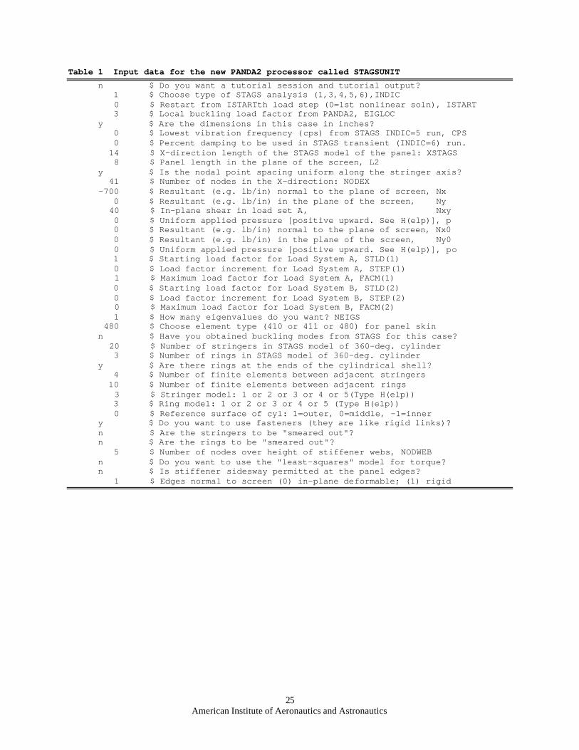
25American Institute of Aeronautics and Astronautics
Table 1 Input data for the new PANDA2 processor called STAGSUNIT n $ Do you want a tutorial session and tutorial output? 1 $ Choose type of STAGS analysis (1,3,4,5,6),INDIC 0 $ Restart from ISTARTth load step (0=1st nonlinear soln), ISTART 3 $ Local buckling load factor from PANDA2, EIGLOC y $ Are the dimensions in this case in inches? 0 $ Lowest vibration frequency (cps) from STAGS INDIC=5 run, CPS 0 $ Percent damping to be used in STAGS transient (INDIC=6) run. 14 $ X-direction length of the STAGS model of the panel: XSTAGS 8 $ Panel length in the plane of the screen, L2 y $ Is the nodal point spacing uniform along the stringer axis? 41 $ Number of nodes in the X-direction: NODEX -700 $ Resultant (e.g. lb/in) normal to the plane of screen, Nx 0 $ Resultant (e.g. lb/in) in the plane of the screen, Ny 40 $ In-plane shear in load set A, Nxy 0 $ Uniform applied pressure [positive upward. See H(elp)], p 0 $ Resultant (e.g. lb/in) normal to the plane of screen, Nx0 0 $ Resultant (e.g. lb/in) in the plane of the screen, Ny0 0 $ Uniform applied pressure [positive upward. See H(elp)], po 1 $ Starting load factor for Load System A, STLD(1) 0 $ Load factor increment for Load System A, STEP(1) 1 $ Maximum load factor for Load System A, FACM(1) 0 $ Starting load factor for Load System B, STLD(2) 0 $ Load factor increment for Load System B, STEP(2) 0 $ Maximum load factor for Load System B, FACM(2) 1 $ How many eigenvalues do you want? NEIGS 480 $ Choose element type (410 or 411 or 480) for panel skin n $ Have you obtained buckling modes from STAGS for this case? 20 $ Number of stringers in STAGS model of 360-deg. cylinder 3 $ Number of rings in STAGS model of 360-deg. cylinder y $ Are there rings at the ends of the cylindrical shell? 4 $ Number of finite elements between adjacent stringers 10 $ Number of finite elements between adjacent rings 3 $ Stringer model: 1 or 2 or 3 or 4 or 5(Type H(elp)) 3 $ Ring model: 1 or 2 or 3 or 4 or 5 (Type H(elp)) 0 $ Reference surface of cyl: 1=outer, 0=middle, -1=inner y $ Do you want to use fasteners (they are like rigid links)? n $ Are the stringers to be "smeared out"? n $ Are the rings to be "smeared out"? 5 $ Number of nodes over height of stiffener webs, NODWEB n $ Do you want to use the "least-squares" model for torque? n $ Is stiffener sidesway permitted at the panel edges? 1 $ Edges normal to screen (0) in-plane deformable; (1) rigid
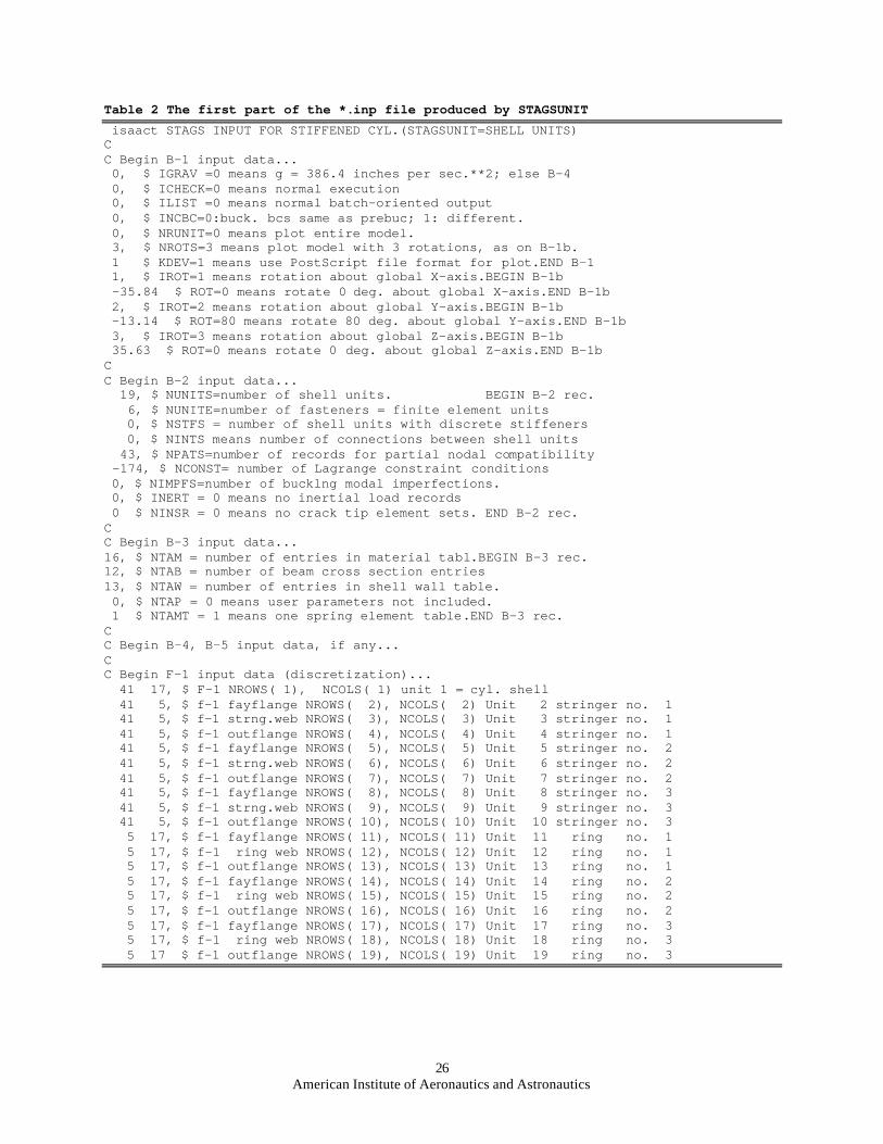
26American Institute of Aeronautics and Astronautics
Table 2 The first part of the *.inp file produced by STAGSUNIT isaact STAGS INPUT FOR STIFFENED CYL.(STAGSUNIT=SHELL UNITS)CC Begin B-1 input data... 0, $ IGRAV =0 means g = 386.4 inches per sec.**2; else B-4 0, $ ICHECK=0 means normal execution 0, $ ILIST =0 means normal batch-oriented output 0, $ INCBC=0:buck. bcs same as prebuc; 1: different. 0, $ NRUNIT=0 means plot entire model. 3, $ NROTS=3 means plot model with 3 rotations, as on B-1b. 1 $ KDEV=1 means use PostScript file format for plot.END B-1 1, $ IROT=1 means rotation about global X-axis.BEGIN B-1b -35.84 $ ROT=0 means rotate 0 deg. about global X-axis.END B-1b 2, $ IROT=2 means rotation about global Y-axis.BEGIN B-1b -13.14 $ ROT=80 means rotate 80 deg. about global Y-axis.END B-1b 3, $ IROT=3 means rotation about global Z-axis.BEGIN B-1b 35.63 $ ROT=0 means rotate 0 deg. about global Z-axis.END B-1bCC Begin B-2 input data... 19, $ NUNITS=number of shell units. BEGIN B-2 rec. 6, $ NUNITE=number of fasteners = finite element units 0, $ NSTFS = number of shell units with discrete stiffeners 0, $ NINTS means number of connections between shell units 43, $ NPATS=number of records for partial nodal compatibility -174, $ NCONST= number of Lagrange constraint conditions 0, $ NIMPFS=number of bucklng modal imperfections. 0, $ INERT = 0 means no inertial load records 0 $ NINSR = 0 means no crack tip element sets. END B-2 rec.CC Begin B-3 input data...16, $ NTAM = number of entries in material tabl.BEGIN B-3 rec.12, $ NTAB = number of beam cross section entries13, $ NTAW = number of entries in shell wall table. 0, $ NTAP = 0 means user parameters not included. 1 $ NTAMT = 1 means one spring element table.END B-3 rec.CC Begin B-4, B-5 input data, if any...CC Begin F-1 input data (discretization)... 41 17, $ F-1 NROWS( 1), NCOLS( 1) unit 1 = cyl. shell 41 5, $ f-1 fayflange NROWS( 2), NCOLS( 2) Unit 2 stringer no. 1 41 5, $ f-1 strng.web NROWS( 3), NCOLS( 3) Unit 3 stringer no. 1 41 5, $ f-1 outflange NROWS( 4), NCOLS( 4) Unit 4 stringer no. 1 41 5, $ f-1 fayflange NROWS( 5), NCOLS( 5) Unit 5 stringer no. 2 41 5, $ f-1 strng.web NROWS( 6), NCOLS( 6) Unit 6 stringer no. 2 41 5, $ f-1 outflange NROWS( 7), NCOLS( 7) Unit 7 stringer no. 2 41 5, $ f-1 fayflange NROWS( 8), NCOLS( 8) Unit 8 stringer no. 3 41 5, $ f-1 strng.web NROWS( 9), NCOLS( 9) Unit 9 stringer no. 3 41 5, $ f-1 outflange NROWS( 10), NCOLS( 10) Unit 10 stringer no. 3 5 17, $ f-1 fayflange NROWS( 11), NCOLS( 11) Unit 11 ring no. 1 5 17, $ f-1 ring web NROWS( 12), NCOLS( 12) Unit 12 ring no. 1 5 17, $ f-1 outflange NROWS( 13), NCOLS( 13) Unit 13 ring no. 1 5 17, $ f-1 fayflange NROWS( 14), NCOLS( 14) Unit 14 ring no. 2 5 17, $ f-1 ring web NROWS( 15), NCOLS( 15) Unit 15 ring no. 2 5 17, $ f-1 outflange NROWS( 16), NCOLS( 16) Unit 16 ring no. 2 5 17, $ f-1 fayflange NROWS( 17), NCOLS( 17) Unit 17 ring no. 3 5 17, $ f-1 ring web NROWS( 18), NCOLS( 18) Unit 18 ring no. 3 5 17 $ f-1 outflange NROWS( 19), NCOLS( 19) Unit 19 ring no. 3
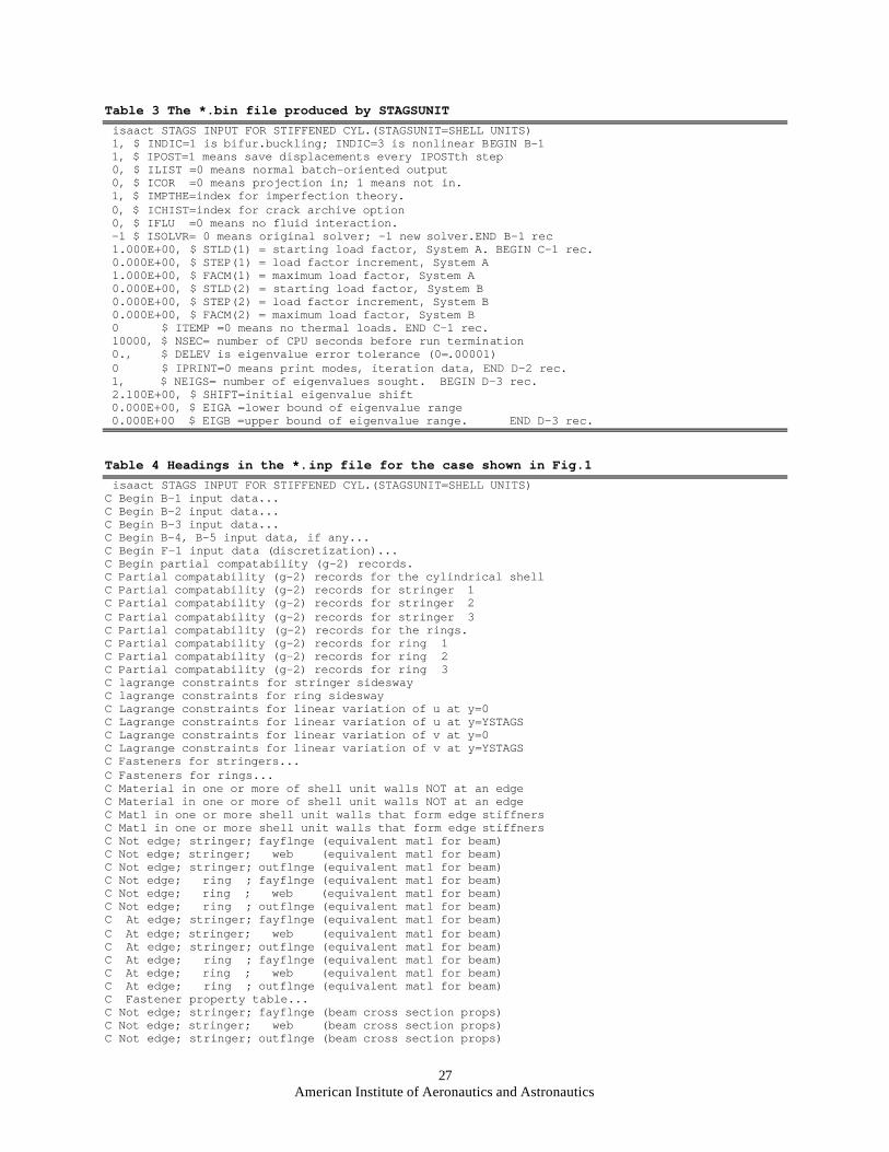
27American Institute of Aeronautics and Astronautics
Table 3 The *.bin file produced by STAGSUNIT isaact STAGS INPUT FOR STIFFENED CYL.(STAGSUNIT=SHELL UNITS) 1, $ INDIC=1 is bifur.buckling; INDIC=3 is nonlinear BEGIN B-1 1, $ IPOST=1 means save displacements every IPOSTth step 0, $ ILIST =0 means normal batch-oriented output 0, $ ICOR =0 means projection in; 1 means not in. 1, $ IMPTHE=index for imperfection theory. 0, $ ICHIST=index for crack archive option 0, $ IFLU =0 means no fluid interaction. -1 $ ISOLVR= 0 means original solver; -1 new solver.END B-1 rec 1.000E+00, $ STLD(1) = starting load factor, System A. BEGIN C-1 rec. 0.000E+00, $ STEP(1) = load factor increment, System A 1.000E+00, $ FACM(1) = maximum load factor, System A 0.000E+00, $ STLD(2) = starting load factor, System B 0.000E+00, $ STEP(2) = load factor increment, System B 0.000E+00, $ FACM(2) = maximum load factor, System B 0 $ ITEMP =0 means no thermal loads. END C-1 rec. 10000, $ NSEC= number of CPU seconds before run termination 0., $ DELEV is eigenvalue error tolerance (0=.00001) 0 $ IPRINT=0 means print modes, iteration data, END D-2 rec. 1, $ NEIGS= number of eigenvalues sought. BEGIN D-3 rec. 2.100E+00, $ SHIFT=initial eigenvalue shift 0.000E+00, $ EIGA =lower bound of eigenvalue range 0.000E+00 $ EIGB =upper bound of eigenvalue range. END D-3 rec.
Table 4 Headings in the *.inp file for the case shown in Fig.1 isaact STAGS INPUT FOR STIFFENED CYL.(STAGSUNIT=SHELL UNITS)C Begin B-1 input data...C Begin B-2 input data...C Begin B-3 input data...C Begin B-4, B-5 input data, if any...C Begin F-1 input data (discretization)...C Begin partial compatability (g-2) records.C Partial compatability (g-2) records for the cylindrical shellC Partial compatability (g-2) records for stringer 1C Partial compatability (g-2) records for stringer 2C Partial compatability (g-2) records for stringer 3C Partial compatability (g-2) records for the rings.C Partial compatability (g-2) records for ring 1C Partial compatability (g-2) records for ring 2C Partial compatability (g-2) records for ring 3C lagrange constraints for stringer sideswayC lagrange constraints for ring sideswayC Lagrange constraints for linear variation of u at y=0C Lagrange constraints for linear variation of u at y=YSTAGSC Lagrange constraints for linear variation of v at y=0C Lagrange constraints for linear variation of v at y=YSTAGSC Fasteners for stringers...C Fasteners for rings...C Material in one or more of shell unit walls NOT at an edgeC Material in one or more of shell unit walls NOT at an edgeC Matl in one or more shell unit walls that form edge stiffnersC Matl in one or more shell unit walls that form edge stiffnersC Not edge; stringer; fayflnge (equivalent matl for beam)C Not edge; stringer; web (equivalent matl for beam)C Not edge; stringer; outflnge (equivalent matl for beam)C Not edge; ring ; fayflnge (equivalent matl for beam)C Not edge; ring ; web (equivalent matl for beam)C Not edge; ring ; outflnge (equivalent matl for beam)C At edge; stringer; fayflnge (equivalent matl for beam)C At edge; stringer; web (equivalent matl for beam)C At edge; stringer; outflnge (equivalent matl for beam)C At edge; ring ; fayflnge (equivalent matl for beam)C At edge; ring ; web (equivalent matl for beam)C At edge; ring ; outflnge (equivalent matl for beam)C Fastener property table...C Not edge; stringer; fayflnge (beam cross section props)C Not edge; stringer; web (beam cross section props)C Not edge; stringer; outflnge (beam cross section props)
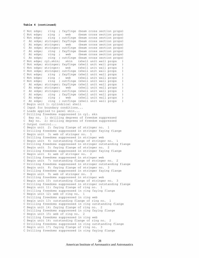
28American Institute of Aeronautics and Astronautics
Table 4 (continued)
C Not edge; ring ; fayflnge (beam cross section props)C Not edge; ring ; web (beam cross section props)C Not edge; ring ; outflnge (beam cross section props)C At edge; stringer; fayflnge (beam cross section props)C At edge; stringer; web (beam cross section props)C At edge; stringer; outflnge (beam cross section props)C At edge; ring ; fayflnge (beam cross section props)C At edge; ring ; web (beam cross section props)C At edge; ring ; outflnge (beam cross section props)C Not edge; cyl.skin; skin (shell unit wall props )C Not edge; stringer; fayflnge (shell unit wall props )C Not edge; stringer; web (shell unit wall props )C Not edge; stringer; outflnge (shell unit wall props )C Not edge; ring ; fayflnge (shell unit wall props )C Not edge; ring ; web (shell unit wall props )C Not edge; ring ; outflnge (shell unit wall props )C At edge; stringer; fayflnge (shell unit wall props )C At edge; stringer; web (shell unit wall props )C At edge; stringer; outflnge (shell unit wall props )C At edge; ring ; fayflnge (shell unit wall props )C At edge; ring ; web (shell unit wall props )C At edge; ring ; outflnge (shell unit wall props )C Begin unit 1: cylindrical shellC Input for boundary conditions...C Loads applied to panel skin...C Drilling freedoms suppressed in cyl. sknC Bay no. 1; drilling degrees of freedom suppressedC Bay no. 2; drilling degrees of freedom suppressedC Output control...C Begin unit 2: faying flange of stringer no. 1C Drilling freedoms suppressed in stringer faying flangeC Begin unit 3: web of stringer no. 1C Drilling freedoms suppressed in stringer webC Begin unit 4: outstanding flange of stringer no. 1C Drilling freedoms suppressed in stringer outstanding flangeC Begin unit 5: faying flange of stringer no. 2C Drilling freedoms suppressed in stringer faying flangeC Begin unit 6: web of stringer no. 2C Drilling freedoms suppressed in stringer webC Begin unit 7: outstanding flange of stringer no. 2C Drilling freedoms suppressed in stringer outstanding flangeC Begin unit 8: faying flange of stringer no. 3C Drilling freedoms suppressed in stringer faying flangeC Begin unit 9: web of stringer no. 3C Drilling freedoms suppressed in stringer webC Begin unit 10: outstanding flange of stringer no. 3C Drilling freedoms suppressed in stringer outstanding flangeC Begin unit 11: faying flange of ring no. 1C Drilling freedoms suppressed in ring faying flangeC Begin unit 12: web of ring no. 1C Drilling freedoms suppressed in ring webC Begin unit 13: outstanding flange of ring no. 1C Drilling freedoms suppressed in ring outstanding flangeC Begin unit 14: faying flange of ring no. 2C Drilling freedoms suppressed in ring faying flangeC Begin unit 15: web of ring no. 2C Drilling freedoms suppressed in ring webC Begin unit 16: outstanding flange of ring no. 2C Drilling freedoms suppressed in ring outstanding flangeC Begin unit 17: faying flange of ring no. 3C Drilling freedoms suppressed in ring faying flange
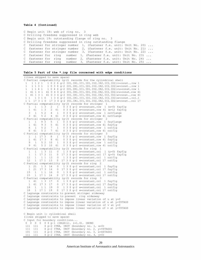
29American Institute of Aeronautics and Astronautics
Table 4 (Continued)
C Begin unit 18: web of ring no. 3C Drilling freedoms suppressed in ring webC Begin unit 19: outstanding flange of ring no. 3C Drilling freedoms suppressed in ring outstanding flangeC fastener for stringer number 1, (fastener f.e. unit: Unit No. 20) ...C fastener for stringer number 2, (fastener f.e. unit: Unit No. 21) ...C fastener for stringer number 3, (fastener f.e. unit: Unit No. 22) ...C fastener for ring number 1, (Fastener f.e. unit: Unit No. 23) ...C fastener for ring number 2, (Fastener f.e. unit: Unit No. 24) ...C fastener for ring number 3, (Fastener f.e. unit: Unit No. 25) ...
Table 5 Part of the *.inp file concerned with edge conditions(lines skipped to save space)C Partial compatability (g-2) records for the cylindrical shell 1 1 1 2 1 1 0 2 $ g-2 IU1,IR1,IC1,ID1,IU2,IR2,IC2,ID2;v=const.,row 1 1 1 1 3 1 1 0 3 $ g-2 IU1,IR1,IC1,ID1,IU2,IR2,IC2,ID2;w=const.,row 1 1 1 1 4 1 1 0 4 $ g-2 IU1,IR1,IC1,ID1,IU2,IR2,IC2,ID2;ru=const,row 1 1 41 1 4 1 41 0 4 $ g-2 IU1,IR1,IC1,ID1,IU2,IR2,IC2,ID2;ru=const,row 41 1 41 1 3 1 41 0 3 $ g-2 IU1,IR1,IC1,ID1,IU2,IR2,IC2,ID2;w=const.,row 41 1 1 1 3 1 0 1 3 $ g-2 IU1,IR1,IC1,ID1,IU2,IR2,IC2,ID2;w=const.,col.1 1 1 17 3 1 0 17 3 $ g-2 IU1,IR1,IC1,ID1,IU2,IR2,IC2,ID2;w=const.,col 17C Partial compatability (g-2) records for stringer 1 1 1 1 3 2 1 0 3 $ g-2 w=constant,row 1 (x=0) fayflg 1 41 1 3 2 41 0 3 $ g-2 w=constant,row 41 (x=L) fayflg 3 1 5 2 4 1 0 3 $ g-2 w=constant,row 1 outflange 3 41 5 2 4 41 0 3 $ g-2 w=constant,row 41 outflangeC Partial compatability (g-2) records for stringer 2 1 1 9 3 5 1 0 3 $ g-2 w=constant,row 1 fayflange 1 41 9 3 5 41 0 3 $ g-2 w=constant,row 41 fayflg 6 1 5 2 7 1 0 3 $ g-2 w=constant,row 1 outflg 6 41 5 2 7 41 0 3 $ g-2 w=constant,row 41 outflgC Partial compatability (g-2) records for stringer 3 1 1 17 3 8 1 0 3 $ g-2 w=constant,row 1 fayflg 1 41 17 3 8 41 0 3 $ g-2 w=constant,row 41 fayflg 9 1 5 2 10 1 0 3 $ g-2 w=constant,row 1 outflg 9 41 5 2 10 41 0 3 $ g-2 w=constant,row 41 outflgC Partial compatability (g-2) records for ring 1 1 1 1 3 11 0 1 3 $ g-2 w=constant,col 1 (y=0) fayflg 1 1 17 3 11 0 17 3 $ g-2 w=constant,col 17 (y=Y) fayflg 12 1 1 1 13 0 1 3 $ g-2 w=constant,col 1 outflg 12 1 17 1 13 0 17 3 $ g-2 w=constant,col 17 outflgC Partial compatability (g-2) records for ring 2 1 21 1 3 14 0 1 3 $ g-2 w=constant,col 1 fayflg 1 21 17 3 14 0 17 3 $ g-2 w=constant,col 17 fayflg 15 1 1 1 16 0 1 3 $ g-2 w=constant,col 1 outflg 15 1 17 1 16 0 17 3 $ g-2 w=constant,col 17 outflgC Partial compatability (g-2) records for ring 3 1 41 1 3 17 0 1 3 $ g-2 w=constant,col 1 fayflg 1 41 17 3 17 0 17 3 $ g-2 w=constant,col 17 fayflg 18 1 1 1 19 0 1 3 $ g-2 w=constant,col 1 outflg 18 1 17 1 19 0 17 3 $ g-2 w=constant,col 17 outflgC lagrange constraints to prevent stringer sideswayC lagrange constraints to prevent ring sideswayC Lagrange constraints to impose linear variation of u at y=0C Lagrange constraints to impose linear variation of u at y=YSTAGSC Lagrange constraints to impose linear variation of v at y=0C Lagrange constraints to impose linear variation of v at y=YSTAGS
C Begin unit 1: cylindrical shell(lines skipped to save space)C Input for boundary conditions... 0 0 0 0 0 $ p-1 (IBLN(i), i=1,4), IBOND 111 111 $ p-2 ITRA, IROT (boundary no. 1, x=0) 111 111 $ p-2 ITRA, IROT (boundary no. 2, y=YSTAGS) 101 111 $ p-2 ITRA, IROT (boundary no. 3, x=XSTAGS) 111 111 $ p-2 ITRA, IROT (boundary no. 4, y=0)
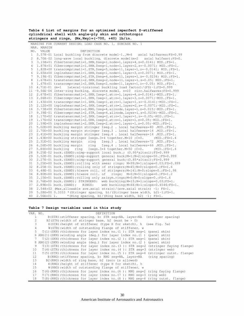
30American Institute of Aeronautics and Astronautics
Table 6 List of margins for an optimized imperfect Z-stiffenedcylindrical shell with angle-ply skin and orthotropicstringers and rings, (Nx,Nxy)=(-700, +40) lb/in. MARGINS FOR CURRENT DESIGN: LOAD CASE NO. 1, SUBCASE NO. 1 MAR. MARGIN NO. VALUE DEFINITION 1 5.57E-01 Local buckling from discrete model-1.,M=6 axial halfwaves;FS=0.99 2 8.70E-02 long-wave local buckling, discrete model(m=2 axial halfwav);FS=0. 3 3.15E+01 fibertensn:matl=1,SKN,Dseg=1,node=1,layer=4,z=0.0141; MID.;FS=1. 4 1.87E+01 fibercompr:matl=1,SKN,Dseg=1,node=1,layer=2,z=-0.0071; MID.;FS=1. 5 1.82E+00 transcompr:matl=1,STR,Dseg=5,node=11,layer=1,z=-0.0141; MID.;FS=1. 6 2.65E+00 inplnshear:matl=1,SKN,Dseg=1,node=1,layer=3,z=0.0071; MID.;FS=1. 7 9.19E-01 fibercompr:matl=2,STR,Dseg=4,node=11,layer=1,z=-0.0234; MID.;FS=1. 8 1.67E+01 transtensn:matl=2,SKN,Dseg=2,node=11,layer=1,z=0.05; MID.;FS=1. 9 1.67E+01 transcompr:matl=2,SKN,Dseg=2,node=11,layer=1,z=-0.05; MID.;FS=1.10 4.71E-01 (m=1 lateral-torsional buckling load factor)/(FS)-1;FS=0.99911 -9.56E-04 Inter-ring bucklng, discrete model, n=10 circ.halfwaves;FS=0.99912 2.67E+01 fibertensn:matl=1,SKN,Iseg=1,at:n=1,layer=4,z=0.0141;-MID.;FS=1.13 2.06E+01 fibercompr:matl=1,SKN,Iseg=1,at:n=1,layer=3,z=0.0071;-MID.;FS=1.14 1.43E+00 transcompr:matl=1,SKN,Iseg=1,at:n=1,layer=1,z=-0.0141;-MID.;FS=1.15 2.12E+00 inplnshear:matl=1,SKN,Iseg=1,at:n=1,layer=2,z=-0.0071;-MID.;FS=1.16 3.73E+00 fibertensn:matl=2,RNG,Iseg=4,allnode,layer=1,z=0.015;-MID.;FS=1.17 9.39E-01 fibercompr:matl=2,STR,Iseg=4,allnode,layer=1,z=0.0234;-MID.;FS=1.18 1.17E+02 transtensn:matl=2,SKN,Iseg=2,at:n=1,layer=1,z=-0.05;-MID.;FS=1.19 1.17E+02 transcompr:matl=2,SKN,Iseg=2,at:n=1,layer=1,z=0.05;-MID.;FS=1.20 1.59E+05 inplnshear:matl=2,SKN,Iseg=2,at:n=1,layer=1,z=0.05;-MID.;FS=1.21 5.02E+00 buckling margin stringer Iseg.2 . Local halfwaves=80 .MID.;FS=1.22 2.70E+00 buckling margin stringer Iseg.3 . Local halfwaves=14 .MID.;FS=1.23 2.41E+00 buckling margin stringer Iseg.4 . Local halfwaves=14 .MID.;FS=1.24 1.43E+00 buckling stringer Isegs.3+4 together.M=10 ;C=0. ;MID.;FS=1.425 2.31E+01 buckling margin ring Iseg.3 . Local halfwaves=72 .MID.;FS=1.26 6.26E+00 buckling margin ring Iseg.4 . Local halfwaves=66 .MID.;FS=1.27 5.84E+00 buckling ring Isegs.3+4 together.M=50 ;C=0. ;MID.;FS=1.428 9.25E-02 buck.(SAND);simp-support local buck.; (0.95*altsol);FS=0.99929 3.52E-01 buck.(SAND);simp-support general buck;M=1;N=2;slope=50.;FS=0.99930 2.27E-01 buck.(SAND);simp-support general buck;(0.85*altsol);FS=0.99931 3.25E+00 buck.(SAND);rolling with smear rings; M=99;N=1;slope=0.03;FS=0.99932 8.25E-01 buck.(SAND);rolling only of stringers;M=45;N=0;slope=0.;FS=1.633 6.48E-01 buck.(SAND);hiwave roll. of stringers;M=141;N=0;slope=0.;FS=1.9834 8.80E+00 buck.(SAND);hiwave roll. of rings; M=0;N=51;slope=0.;FS=1.235 2.15E+01 buck.(SAND);rolling only axisym.rings;M=0;N=0;slope=0.;FS=1.636 2.76E+00 buck.(SAND); STRINGERS: web buckling;M=15;N=1;slope=0.03;FS=1.37 2.89E+01 buck.(SAND); RINGS: web buckling;M=66;N=1;slope=0.6546;FS=1.38 2.54E+02 (Max.allowable ave.axial strain)/(ave.axial strain) -1; FS=1.39 5.28E+00 0.3333 *(Stringer spacing, b)/(Stringer base width, b2)-1;FS=1.40 2.56E+01 1. *(Ring spacing, b)/(Ring base width, b2) -1; FS=1.
Table 7 Design variables used in this studyVAR. NO. DEFINITION 1 B(STR):stiffener spacing, b: STR seg=NA, layer=NA (stringer spacing) 2 B2(STR):width of stringer base, b2 (must be > 0) 3 H(STR):height of stiffener (type H for sketch), h (see Fig. 5a) 4 W(STR):width of outstanding flange of stiffener, w 5 T(1)(SKN):thickness for layer index no.(1 ): STR seg=1 (panel skin) 6 ANG(1)(SKN):winding angle (deg.) for layer index no.(1 ) (panel skin) 7 T(2)(SKN):thickness for layer index no.(2 ): STR seg=1 (panel skin) 8 ANG(2)(SKN):winding angle (deg.) for layer index no.(2 ) (panel skin) 9 T(3)(STR):thickness for layer index no.(3 ): STR seg=2 (stringer faying flange) 10 T(4)(STR):thickness for layer index no.(4 ): STR seg=3 (stringer web) 11 T(5)(STR):thickness for layer index no.(5 ): STR seg=4 (stringer outst. flange) 12 B(RNG):stiffener spacing, b: RNG seg=NA, layer=NA (ring spacing) 13 B2(RNG):width of ring base, b2 (zero is allowed) 14 H(RNG):height of stiffener (type H for sketch), h 15 W(RNG):width of outstanding flange of stiffener, w 16 T(6)(RNG):thickness for layer index no.(6 ): RNG seg=2 (ring faying flange) 17 T(7)(RNG):thickness for layer index no.(7 ): RNG seg=3 (ring web) 18 T(8)(RNG):thickness for layer index no.(8 ): RNG seg=4 (ring outst. flange)
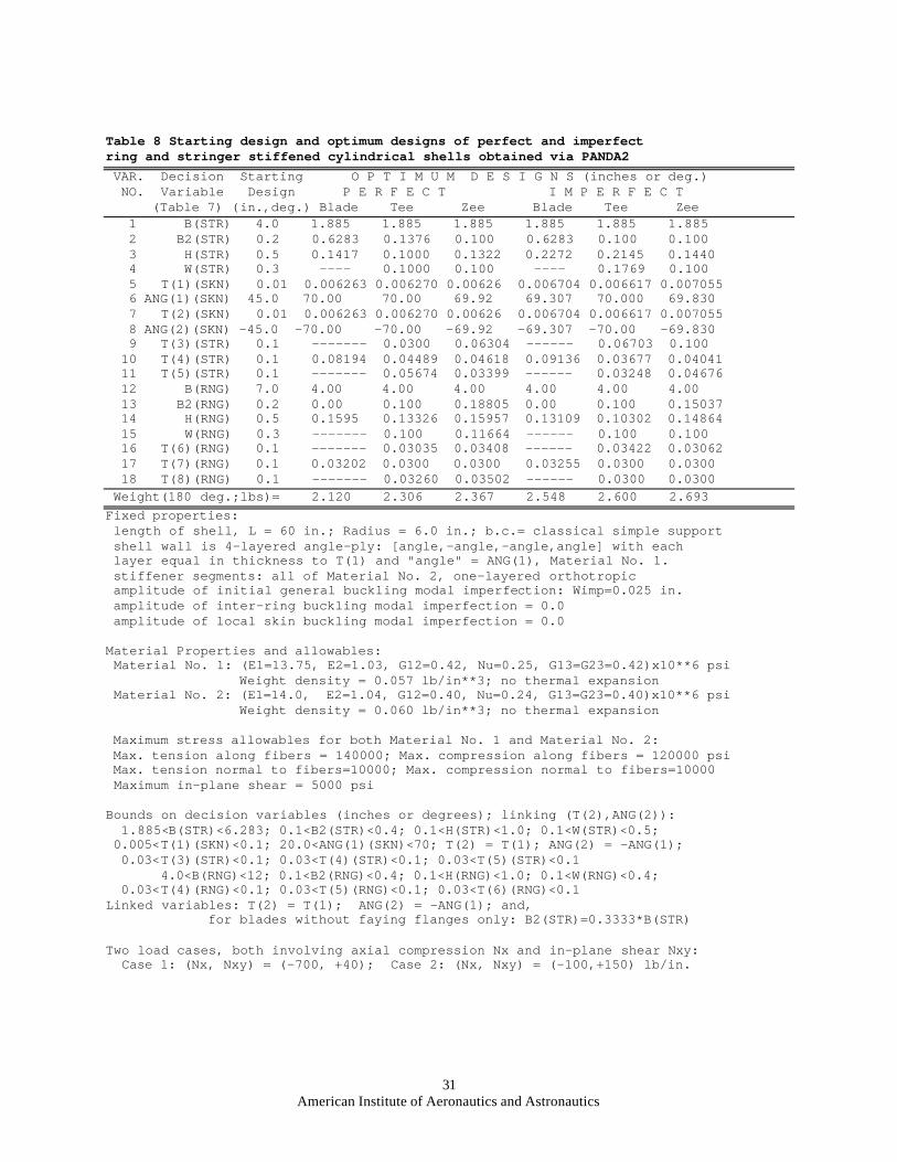
31American Institute of Aeronautics and Astronautics
Table 8 Starting design and optimum designs of perfect and imperfectring and stringer stiffened cylindrical shells obtained via PANDA2 VAR. Decision Starting O P T I M U M D E S I G N S (inches or deg.) NO. Variable Design P E R F E C T I M P E R F E C T (Table 7) (in.,deg.) Blade Tee Zee Blade Tee Zee 1 B(STR) 4.0 1.885 1.885 1.885 1.885 1.885 1.885 2 B2(STR) 0.2 0.6283 0.1376 0.100 0.6283 0.100 0.100 3 H(STR) 0.5 0.1417 0.1000 0.1322 0.2272 0.2145 0.1440 4 W(STR) 0.3 ---- 0.1000 0.100 ---- 0.1769 0.100 5 T(1)(SKN) 0.01 0.006263 0.006270 0.00626 0.006704 0.006617 0.007055 6 ANG(1)(SKN) 45.0 70.00 70.00 69.92 69.307 70.000 69.830 7 T(2)(SKN) 0.01 0.006263 0.006270 0.00626 0.006704 0.006617 0.007055 8 ANG(2)(SKN) -45.0 -70.00 -70.00 -69.92 -69.307 -70.00 -69.830 9 T(3)(STR) 0.1 ------- 0.0300 0.06304 ------ 0.06703 0.100 10 T(4)(STR) 0.1 0.08194 0.04489 0.04618 0.09136 0.03677 0.04041 11 T(5)(STR) 0.1 ------- 0.05674 0.03399 ------ 0.03248 0.04676 12 B(RNG) 7.0 4.00 4.00 4.00 4.00 4.00 4.00 13 B2(RNG) 0.2 0.00 0.100 0.18805 0.00 0.100 0.15037 14 H(RNG) 0.5 0.1595 0.13326 0.15957 0.13109 0.10302 0.14864 15 W(RNG) 0.3 ------- 0.100 0.11664 ------ 0.100 0.100 16 T(6)(RNG) 0.1 ------- 0.03035 0.03408 ------ 0.03422 0.03062 17 T(7)(RNG) 0.1 0.03202 0.0300 0.0300 0.03255 0.0300 0.0300 18 T(8)(RNG) 0.1 ------- 0.03260 0.03502 ------ 0.0300 0.0300 Weight(180 deg.;lbs)= 2.120 2.306 2.367 2.548 2.600 2.693Fixed properties: length of shell, L = 60 in.; Radius = 6.0 in.; b.c.= classical simple support shell wall is 4-layered angle-ply: [angle,-angle,-angle,angle] with each layer equal in thickness to T(1) and "angle" = ANG(1), Material No. 1. stiffener segments: all of Material No. 2, one-layered orthotropic amplitude of initial general buckling modal imperfection: Wimp=0.025 in. amplitude of inter-ring buckling modal imperfection = 0.0 amplitude of local skin buckling modal imperfection = 0.0
Material Properties and allowables: Material No. 1: (E1=13.75, E2=1.03, G12=0.42, Nu=0.25, G13=G23=0.42)x10**6 psi Weight density = 0.057 lb/in**3; no thermal expansion Material No. 2: (E1=14.0, E2=1.04, G12=0.40, Nu=0.24, G13=G23=0.40)x10**6 psi Weight density = 0.060 lb/in**3; no thermal expansion
Maximum stress allowables for both Material No. 1 and Material No. 2: Max. tension along fibers = 140000; Max. compression along fibers = 120000 psi Max. tension normal to fibers=10000; Max. compression normal to fibers=10000 Maximum in-plane shear = 5000 psi
Bounds on decision variables (inches or degrees); linking (T(2),ANG(2)): 1.885<B(STR)<6.283; 0.1<B2(STR)<0.4; 0.1<H(STR)<1.0; 0.1<W(STR)<0.5; 0.005<T(1)(SKN)<0.1; 20.0<ANG(1)(SKN)<70; T(2) = T(1); ANG(2) = -ANG(1); 0.03<T(3)(STR)<0.1; 0.03<T(4)(STR)<0.1; 0.03<T(5)(STR)<0.1 4.0<B(RNG)<12; 0.1<B2(RNG)<0.4; 0.1<H(RNG)<1.0; 0.1<W(RNG)<0.4; 0.03<T(4)(RNG)<0.1; 0.03<T(5)(RNG)<0.1; 0.03<T(6)(RNG)<0.1Linked variables: T(2) = T(1); ANG(2) = -ANG(1); and, for blades without faying flanges only: B2(STR)=0.3333*B(STR)
Two load cases, both involving axial compression Nx and in-plane shear Nxy: Case 1: (Nx, Nxy) = (-700, +40); Case 2: (Nx, Nxy) = (-100,+150) lb/in.
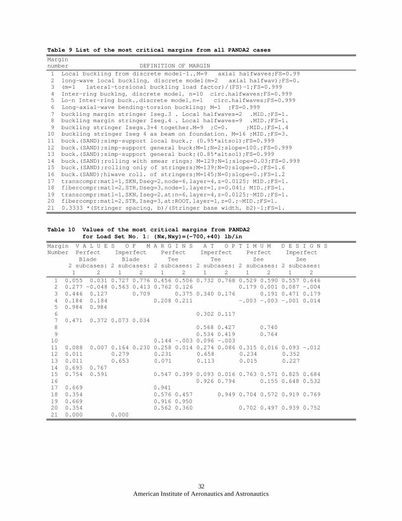
32American Institute of Aeronautics and Astronautics
Table 9 List of the most critical margins from all PANDA2 casesMarginnumber DEFINITION OF MARGIN 1 Local buckling from discrete model-1.,M=9 axial halfwaves;FS=0.99 2 long-wave local buckling, discrete model(m=2 axial halfwav);FS=0. 3 (m=1 lateral-torsional buckling load factor)/(FS)-1;FS=0.999 4 Inter-ring bucklng, discrete model, n=10 circ.halfwaves;FS=0.999 5 Lo-n Inter-ring buck.,discrete model,n=1 circ.halfwaves;FS=0.999 6 Long-axial-wave bending-torsion buckling; M=1 ;FS=0.999 7 buckling margin stringer Iseg.3 . Local halfwaves=2 .MID.;FS=1. 8 buckling margin stringer Iseg.4 . Local halfwaves=9 .MID.;FS=1. 9 buckling stringer Isegs.3+4 together.M=9 ;C=0. ;MID.;FS=1.410 buckling stringer Iseg 4 as beam on foundation. M=16 ;MID.;FS=3.11 buck.(SAND);simp-support local buck.; (0.95*altsol);FS=0.99912 buck.(SAND);simp-support general buck;M=1;N=2;slope=100.;FS=0.99913 buck.(SAND);simp-support general buck;(0.85*altsol);FS=0.99914 buck.(SAND);rolling with smear rings; M=129;N=1;slope=0.03;FS=0.99915 buck.(SAND);rolling only of stringers;M=139;N=0;slope=0.;FS=1.616 buck.(SAND);hiwave roll. of stringers;M=145;N=0;slope=0.;FS=1.217 transcompr:matl=1,SKN,Dseg=2,node=6,layer=4,z=0.0125; MID.;FS=1.18 fibercompr:matl=2,STR,Dseg=3,node=1,layer=1,z=0.041; MID.;FS=1.19 transcompr:matl=1,SKN,Iseg=2,at:n=6,layer=4,z=0.0125;-MID.;FS=1.20 fibercompr:matl=2,STR,Iseg=3,at:ROOT,layer=1,z=0.;-MID.;FS=1.21 0.3333 *(Stringer spacing, b)/(Stringer base width, b2)-1;FS=1.
Table 10 Values of the most critical margins from PANDA2 for Load Set No. 1: (Nx,Nxy)=(-700,+40) lb/inMargin V A L U E S O F M A R G I N S A T O P T I M U M D E S I G N SNumber Perfect Imperfect Perfect Imperfect Perfect Imperfect Blade Blade Tee Tee Zee Zee 2 subcases: 2 subcases: 2 subcases: 2 subcases: 2 subcases: 2 subcases: 1 2 1 2 1 2 1 2 1 2 1 2 1 0.055 0.031 0.727 0.776 0.456 0.506 0.732 0.768 0.529 0.590 0.557 0.646 2 0.277 -0.048 0.563 0.413 0.762 0.126 0.179 0.001 0.087 -.004 3 0.446 0.127 0.709 0.375 0.340 0.176 0.191 0.471 0.179 4 0.184 0.184 0.208 0.211 -.003 -.003 -.001 0.014 5 0.984 0.984 6 0.302 0.117 7 0.471 0.372 0.073 0.034 8 0.568 0.427 0.740 9 0.534 0.419 0.764 10 0.144 -.003 0.096 -.003 11 0.088 0.007 0.164 0.230 0.258 0.014 0.274 0.086 0.315 0.016 0.093 -.012 12 0.011 0.279 0.231 0.658 0.234 0.352 13 0.011 0.653 0.071 0.113 0.015 0.227 14 0.693 0.767 15 0.754 0.591 0.547 0.399 0.093 0.016 0.763 0.571 0.825 0.684 16 0.926 0.794 0.155 0.648 0.532 17 0.669 0.941 18 0.354 0.576 0.457 0.949 0.704 0.572 0.919 0.769 19 0.669 0.916 0.950 20 0.354 0.562 0.360 0.702 0.497 0.939 0.752 21 0.000 0.000
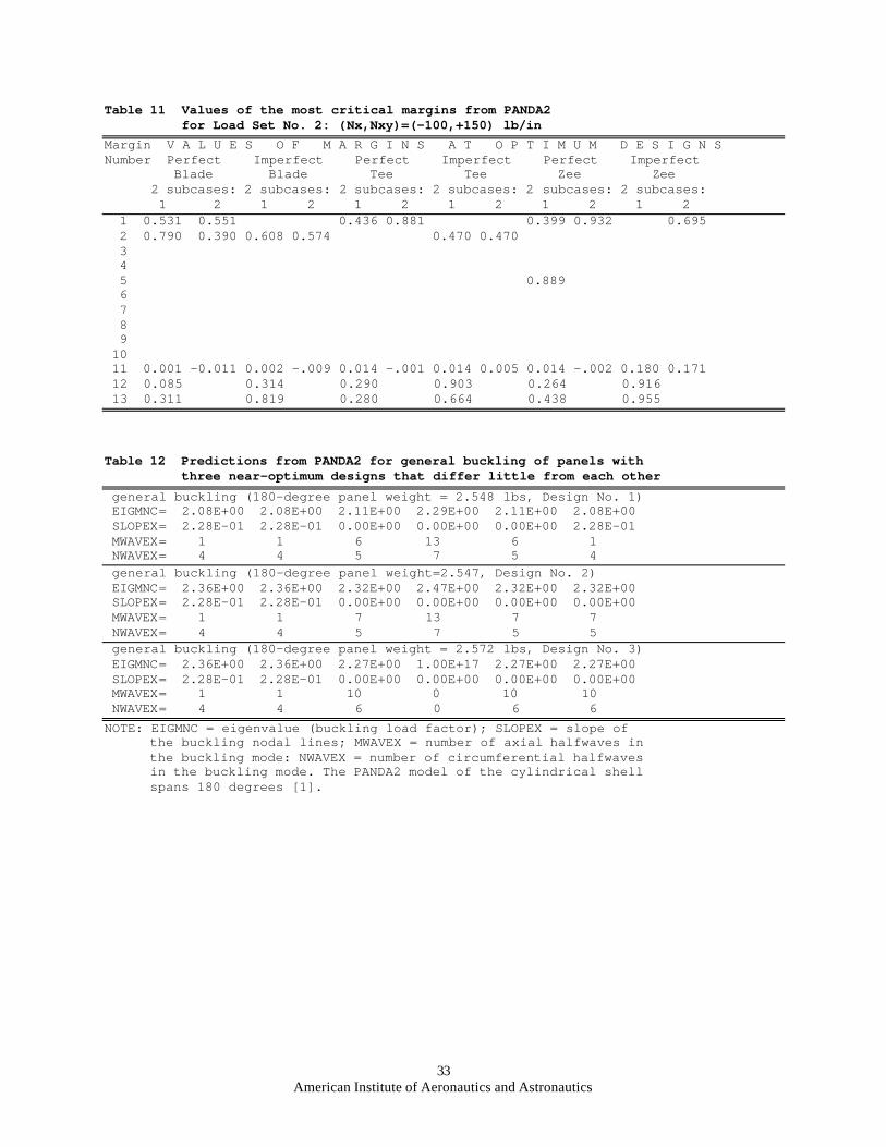
33American Institute of Aeronautics and Astronautics
Table 11 Values of the most critical margins from PANDA2 for Load Set No. 2: (Nx,Nxy)=(-100,+150) lb/inMargin V A L U E S O F M A R G I N S A T O P T I M U M D E S I G N SNumber Perfect Imperfect Perfect Imperfect Perfect Imperfect Blade Blade Tee Tee Zee Zee 2 subcases: 2 subcases: 2 subcases: 2 subcases: 2 subcases: 2 subcases: 1 2 1 2 1 2 1 2 1 2 1 2 1 0.531 0.551 0.436 0.881 0.399 0.932 0.695 2 0.790 0.390 0.608 0.574 0.470 0.470 3 4 5 0.889 6 7 8 9 10 11 0.001 -0.011 0.002 -.009 0.014 -.001 0.014 0.005 0.014 -.002 0.180 0.171 12 0.085 0.314 0.290 0.903 0.264 0.916 13 0.311 0.819 0.280 0.664 0.438 0.955
Table 12 Predictions from PANDA2 for general buckling of panels with three near-optimum designs that differ little from each other general buckling (180-degree panel weight = 2.548 lbs, Design No. 1) EIGMNC= 2.08E+00 2.08E+00 2.11E+00 2.29E+00 2.11E+00 2.08E+00 SLOPEX= 2.28E-01 2.28E-01 0.00E+00 0.00E+00 0.00E+00 2.28E-01 MWAVEX= 1 1 6 13 6 1 NWAVEX= 4 4 5 7 5 4 general buckling (180-degree panel weight=2.547, Design No. 2) EIGMNC= 2.36E+00 2.36E+00 2.32E+00 2.47E+00 2.32E+00 2.32E+00 SLOPEX= 2.28E-01 2.28E-01 0.00E+00 0.00E+00 0.00E+00 0.00E+00 MWAVEX= 1 1 7 13 7 7 NWAVEX= 4 4 5 7 5 5 general buckling (180-degree panel weight = 2.572 lbs, Design No. 3) EIGMNC= 2.36E+00 2.36E+00 2.27E+00 1.00E+17 2.27E+00 2.27E+00 SLOPEX= 2.28E-01 2.28E-01 0.00E+00 0.00E+00 0.00E+00 0.00E+00 MWAVEX= 1 1 10 0 10 10 NWAVEX= 4 4 6 0 6 6NOTE: EIGMNC = eigenvalue (buckling load factor); SLOPEX = slope of the buckling nodal lines; MWAVEX = number of axial halfwaves in the buckling mode: NWAVEX = number of circumferential halfwaves in the buckling mode. The PANDA2 model of the cylindrical shell spans 180 degrees [1].
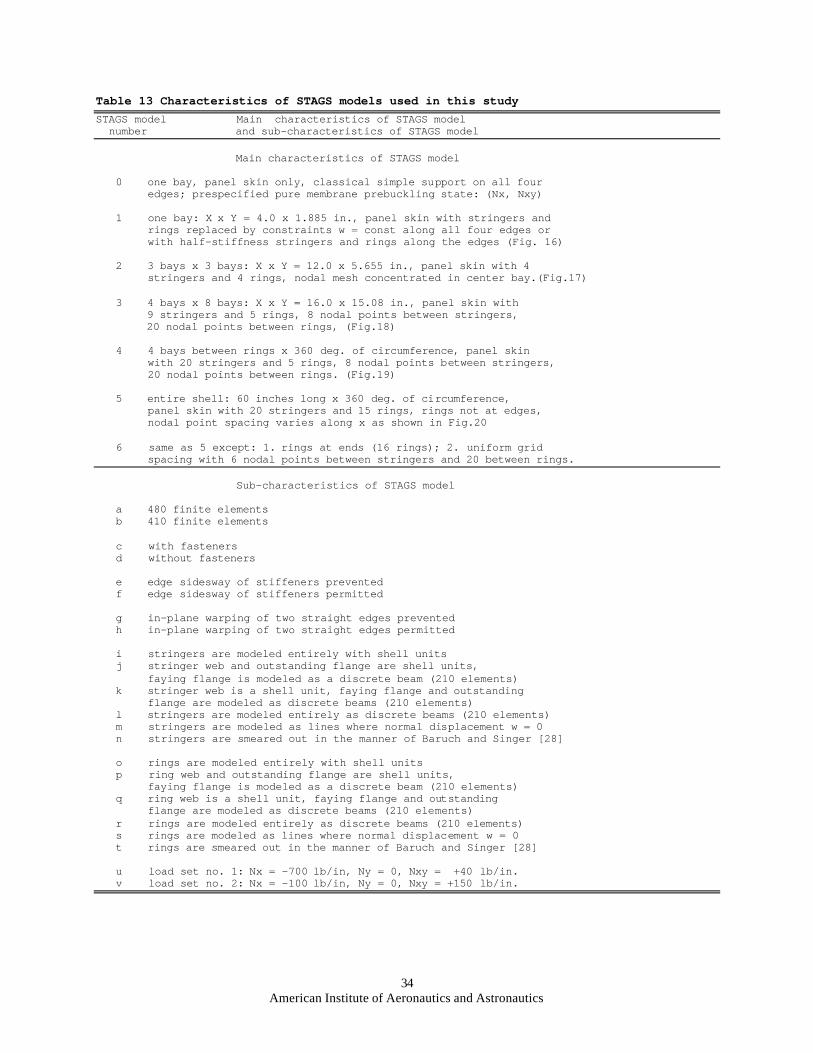
34American Institute of Aeronautics and Astronautics
Table 13 Characteristics of STAGS models used in this studySTAGS model Main characteristics of STAGS model number and sub-characteristics of STAGS model
Main characteristics of STAGS model
0 one bay, panel skin only, classical simple support on all four edges; prespecified pure membrane prebuckling state: (Nx, Nxy)
1 one bay: X x Y = 4.0 x 1.885 in., panel skin with stringers and rings replaced by constraints w = const along all four edges or with half-stiffness stringers and rings along the edges (Fig. 16)
2 3 bays x 3 bays: X x Y = 12.0 x 5.655 in., panel skin with 4 stringers and 4 rings, nodal mesh concentrated in center bay.(Fig.17)
3 4 bays x 8 bays: X x Y = 16.0 x 15.08 in., panel skin with 9 stringers and 5 rings, 8 nodal points between stringers, 20 nodal points between rings, (Fig.18)
4 4 bays between rings x 360 deg. of circumference, panel skin with 20 stringers and 5 rings, 8 nodal points between stringers, 20 nodal points between rings. (Fig.19)
5 entire shell: 60 inches long x 360 deg. of circumference, panel skin with 20 stringers and 15 rings, rings not at edges, nodal point spacing varies along x as shown in Fig.20
6 same as 5 except: 1. rings at ends (16 rings); 2. uniform grid spacing with 6 nodal points between stringers and 20 between rings.
Sub-characteristics of STAGS model
a 480 finite elements b 410 finite elements
c with fasteners d without fasteners
e edge sidesway of stiffeners prevented f edge sidesway of stiffeners permitted
g in-plane warping of two straight edges prevented h in-plane warping of two straight edges permitted
i stringers are modeled entirely with shell units j stringer web and outstanding flange are shell units, faying flange is modeled as a discrete beam (210 elements) k stringer web is a shell unit, faying flange and outstanding flange are modeled as discrete beams (210 elements) l stringers are modeled entirely as discrete beams (210 elements) m stringers are modeled as lines where normal displacement w = 0 n stringers are smeared out in the manner of Baruch and Singer [28]
o rings are modeled entirely with shell units p ring web and outstanding flange are shell units, faying flange is modeled as a discrete beam (210 elements) q ring web is a shell unit, faying flange and outstanding flange are modeled as discrete beams (210 elements) r rings are modeled entirely as discrete beams (210 elements) s rings are modeled as lines where normal displacement w = 0 t rings are smeared out in the manner of Baruch and Singer [28]
u load set no. 1: Nx = -700 lb/in, Ny = 0, Nxy = +40 lb/in. v load set no. 2: Nx = -100 lb/in, Ny = 0, Nxy = +150 lb/in.
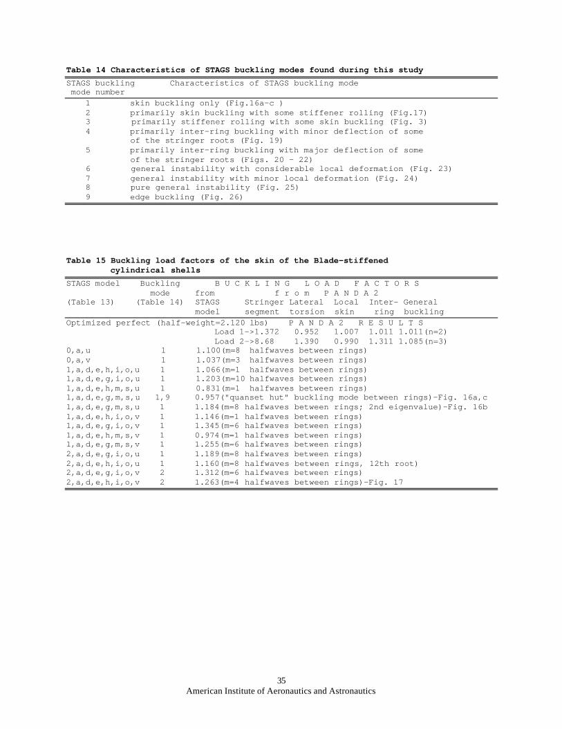
35American Institute of Aeronautics and Astronautics
Table 14 Characteristics of STAGS buckling modes found during this studySTAGS buckling Characteristics of STAGS buckling mode mode number 1 skin buckling only (Fig.16a-c ) 2 primarily skin buckling with some stiffener rolling (Fig.17) 3 primarily stiffener rolling with some skin buckling (Fig. 3) 4 primarily inter-ring buckling with minor deflection of some of the stringer roots (Fig. 19) 5 primarily inter-ring buckling with major deflection of some of the stringer roots (Figs. 20 - 22) 6 general instability with considerable local deformation (Fig. 23) 7 general instability with minor local deformation (Fig. 24) 8 pure general instability (Fig. 25) 9 edge buckling (Fig. 26)
Table 15 Buckling load factors of the skin of the Blade-stiffened cylindrical shellsSTAGS model Buckling B U C K L I N G L O A D F A C T O R S mode from f r o m P A N D A 2(Table 13) (Table 14) STAGS Stringer Lateral Local Inter- General model segment torsion skin ring bucklingOptimized perfect (half-weight=2.120 lbs) P A N D A 2 R E S U L T S Load 1->1.372 0.952 1.007 1.011 1.011(n=2) Load 2->8.68 1.390 0.990 1.311 1.085(n=3)0,a,u 1 1.100(m=8 halfwaves between rings)0,a,v 1 1.037(m=3 halfwaves between rings)1,a,d,e,h,i,o,u 1 1.066(m=1 halfwaves between rings)1,a,d,e,g,i,o,u 1 1.203(m=10 halfwaves between rings)1,a,d,e,h,m,s,u 1 0.831(m=1 halfwaves between rings)1,a,d,e,g,m,s,u 1,9 0.957("quanset hut" buckling mode between rings)-Fig. 16a,c1,a,d,e,g,m,s,u 1 1.184(m=8 halfwaves between rings; 2nd eigenvalue)–Fig. 16b1,a,d,e,h,i,o,v 1 1.146(m=1 halfwaves between rings)1,a,d,e,g,i,o,v 1 1.345(m=6 halfwaves between rings)1,a,d,e,h,m,s,v 1 0.974(m=1 halfwaves between rings)1,a,d,e,g,m,s,v 1 1.255(m=6 halfwaves between rings)2,a,d,e,g,i,o,u 1 1.189(m=8 halfwaves between rings)2,a,d,e,h,i,o,u 1 1.160(m=8 halfwaves between rings, 12th root)2,a,d,e,g,i,o,v 2 1.312(m=6 halfwaves between rings)2,a,d,e,h,i,o,v 2 1.263(m=4 halfwaves between rings)-Fig. 17
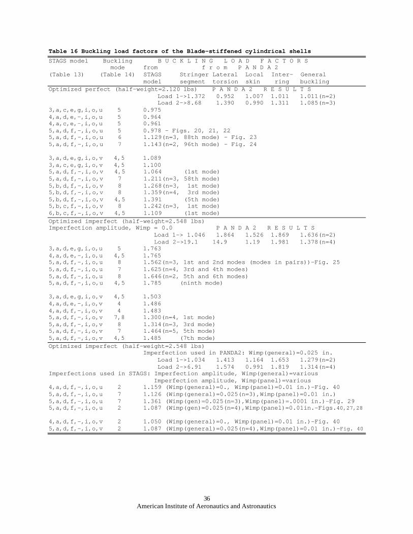
36American Institute of Aeronautics and Astronautics
Table 16 Buckling load factors of the Blade-stiffened cylindrical shellsSTAGS model Buckling B U C K L I N G L O A D F A C T O R S mode from f r o m P A N D A 2(Table 13) (Table 14) STAGS Stringer Lateral Local Inter- General model segment torsion skin ring bucklingOptimized perfect (half-weight=2.120 lbs) P A N D A 2 R E S U L T S Load 1->1.372 0.952 1.007 1.011 1.011(n=2) Load 2->8.68 1.390 0.990 1.311 1.085(n=3)3,a,c,e,g,i,o,u 5 0.9754,a,d,e,-,i,o,u 5 0.9644,a,c,e,-,i,o,u 5 0.9615,a,d,f,-,i,o,u 5 0.978 – Figs. 20, 21, 225,a,d,f,-,i,o,u 6 1.129(n=3, 88th mode) - Fig. 235,a,d,f,-,i,o,u 7 1.143(n=2, 96th mode) – Fig. 24
3,a,d,e,g,i,o,v 4,5 1.0893,a,c,e,g,i,o,v 4,5 1.1005,a,d,f,-,i,o,v 4,5 1.064 (1st mode)5,a,d,f,-,i,o,v 7 1.211(n=3, 58th mode)5,b,d,f,-,i,o,v 8 1.268(n=3, 1st mode)5,b,d,f,-,i,o,v 8 1.359(n=4, 3rd mode)5,b,d,f,-,i,o,v 4,5 1.391 (5th mode)5,b,c,f,-,i,o,v 8 1.242(n=3, 1st mode)6,b,c,f,-,i,o,v 4,5 1.109 (1st mode)Optimized imperfect (half-weight=2.548 lbs)Imperfection amplitude, Wimp = 0.0 P A N D A 2 R E S U L T S Load 1-> 1.046 1.864 1.526 1.869 1.636(n=2) Load 2->19.1 14.9 1.19 1.981 1.378(n=4)3,a,d,e,g,i,o,u 5 1.7634,a,d,e,-,i,o,u 4,5 1.7655,a,d,f,-,i,o,u 8 1.562(n=3, 1st and 2nd modes (modes in pairs))-Fig. 255,a,d,f,-,i,o,u 7 1.625(n=4, 3rd and 4th modes)5,a,d,f,-,i,o,u 8 1.646(n=2, 5th and 6th modes)5,a,d,f,-,i,o,u 4,5 1.785 (ninth mode)
3,a,d,e,g,i,o,v 4,5 1.5034,a,d,e,-,i,o,v 4 1.4864,a,d,f,-,i,o,v 4 1.4835,a,d,f,-,i,o,v 7,8 1.300(n=4, 1st mode)5,a,d,f,-,i,o,v 8 1.314(n=3, 3rd mode)5,a,d,f,-,i,o,v 7 1.464(n=5, 5th mode)5,a,d,f,-,i,o,v 4,5 1.485 (7th mode)Optimized imperfect (half-weight=2.548 lbs) Imperfection used in PANDA2: Wimp(general)=0.025 in. Load 1->1.034 1.413 1.164 1.653 1.279(n=2) Load 2->6.91 1.574 0.991 1.819 1.314(n=4)Imperfections used in STAGS: Imperfection amplitude, Wimp(general)=various Imperfection amplitude, Wimp(panel)=various4,a,d,f,-,i,o,u 2 1.159 (Wimp(general)=0., Wimp(panel)=0.01 in.)-Fig. 405,a,d,f,-,i,o,u 7 1.126 (Wimp(general)=0.025(n=3),Wimp(panel)=0.01 in.)5,a,d,f,-,i,o,u 7 1.361 (Wimp(gen)=0.025(n=3),Wimp(panel)=.0001 in.)-Fig. 295,a,d,f,-,i,o,u 2 1.087 (Wimp(gen)=0.025(n=4),Wimp(panel)=0.01in.-Figs.40,27,28
4,a,d,f,-,i,o,v 2 1.050 (Wimp(general)=0., Wimp(panel)=0.01 in.)-Fig. 405,a,d,f,-,i,o,v 2 1.087 (Wimp(general)=0.025(n=4),Wimp(panel)=0.01 in.)-Fig. 40
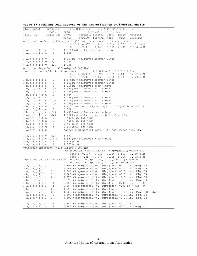
37American Institute of Aeronautics and Astronautics
Table 17 Buckling load factors of the Tee-stiffened cylindrical shellsSTAGS model Buckling B U C K L I N G L O A D F A C T O R S mode from f r o m P A N D A 2(Table 13) (Table 14) STAGS Stringer Lateral Local Inter- General model segment torsion skin ring bucklingOptimized perfect (half-weight=2.306 lbs) P A N D A 2 R E S U L T S Load 1->0.997 1.126 1.014 1.071 1.231(n=2) Load 2->7.05 9.44 0.999 1.280 1.290(n=3)2,a,c,e,g,i,o,u 1 1.385(m=8 halfwaves between rings)3,a,c,e,g,i,o,u 5 1.088
2,a,c,e,g,i,o,v 1 1.337(m=7 halfwaves between rings)3,a,d,e,g,i,o,v 4,5 1.1483,a,c,e,g,i,o,v 4,5 1.155Optimized imperfect (half-weight=2.600 lbs)Imperfection amplitude, Wimp = 0.0 P A N D A 2 R E S U L T S Load 1->0.997 1.020 1.389 1.197 1.967(n=2) Load 2->7.00 7.16 1.150 1.734 1.973(n=3)2,b,d,e,g,l,r,u 1 1.979(m=8 halfwaves between rings)2,b,d,e,g,m,s,u 1 1.812(m=8 halfwaves between rings)3,b,d,e,g,i,o,u 3 1.200(m=6 halfwaves over 4 bays)3,b,c,e,g,i,o,u 2,3 1.448(m=6 halfwaves over 4 bays)3,b,c,e,g,j,p,u 2,3 1.520(m=6 halfwaves over 4 bays)3,b,d,e,g,k,q,u 9 1.6503,a,d,e,g,i,o,u 3 1.170(m=6 halfwaves over 4 bays)3,a,c,e,g,i,o,u 2,3 1.410(m=6 halfwaves over 4 bays)3,a,c,e,h,i,o,u 2,3 1.334(m=5 halfwaves over 4 bays)3,a,d,e,g,i,t,u 3 1.417 (m=7; entirely stringer rolling without skin.)3,a,c,f,g,i,o,u 9 0.9604,b,c,e,-,j,p,u 2,3 1.473(m=6 halfwaves over 4 bays)4,a,c,e,-,i,o,u 2,3 1.360(m=5 halfwaves over 4 bays)-Fig. 19a5,a,d,e,-,n,t,u 8 2.443(n=2, 1st mode)5,b,d,e,-,n,t,u 8 2.496(n=2, 1st mode)5,b,d,e,-,l,r,u 8 2.427(n=2, 1st mode)5,a,d,e,-,n,o,u 8 2.303(n=2, 1st mode)5,a,d,e,-,i,t,u - cannot find general mode: 760 local modes hide it.
3,a,c,e,g,i,o,v 2,3 1.5724,a,c,e,-,i,o,v 2,3,4 1.533(m=5 halfwaves over 4 bays)5,a,d,e,-,i,t,v 8 2.614(n=3)5,a,c,e,-,i,t,v 8 2.587(n=3)Optimized imperfect (half-weight=2.600 lbs) Imperfection used in PANDA2: Wimp(general)=0.025 in. Load 1->0.997 1.016 1.086 1.113 1.658(n=2) Load 2->7.01 1.470 1.005 1.664 1.903(n=3)Imperfections used in STAGS: Imperfection amplitude, Wimp(general)=various Imperfection amplitude, Wimp(panel)=various3,a,d,e,g,i,o,u 2,3 0.899 (Wimp(general)=0., Wimp(panel)=0.01 in.)-Fig. 343,b,d,e,g,i,o,u 2,3 0.901 (Wimp(general)=0., Wimp(panel)=0.01 in.)-Fig. 343,a,c,e,g,i,o,u 2,3 0.905 (Wimp(general)=0., Wimp(panel)=0.01 in.)-Fig. 343,b,c,e,g,i,o,u 2,3 0.940 (Wimp(general)=0., Wimp(panel)=0.01 in.)-Fig. 343,b,c,e,g,j,p,u 2,3 0.970 (Wimp(general)=0., Wimp(panel)=0.01 in.)-Fig. 343,b,d,e,g,k,q,u 9 1.092 (Wimp(general)=0., Wimp(panel)=0.01 in.)-Fig. 342,b,d,e,g,l,r,u 1 1.75 (Wimp(general)=0., Wimp(skin)=0.01 in.)-Fig. 342,a,d,e,g,m,s,u 1 1.18 (Wimp(general)=0., Wimp(skin)=0.01 in.)-Fig. 344,b,c,e,-,j,p,u 2,3 0.990 (Wimp(general)=0., Wimp(panel)=0.01 in.)4,a,c,e,-,i,o,u 2,3 0.920 (Wimp(general)=0., Wimp(panel)=0.01 in.)-Figs. 40,19b,343,a,c,f,g,i,o,u 9 0.800 (Wimp(general)=0., Wimp(panel)=0.01 in.)-Fig. 263,a,c,e,h,i,o,u 2,3 0.890 (Wimp(general)=0., Wimp(panel)=0.01 in.)-Fig. 34
3,a,c,e,g,i,o,v 2 0.940 (Wimp(general)=0., Wimp(panel)=0.01 in.)4.a,c.e.-.i.o,v 2 0.940 (Wimp(general)=0., Wimp(panel)=0.01 in.)-Fig. 40
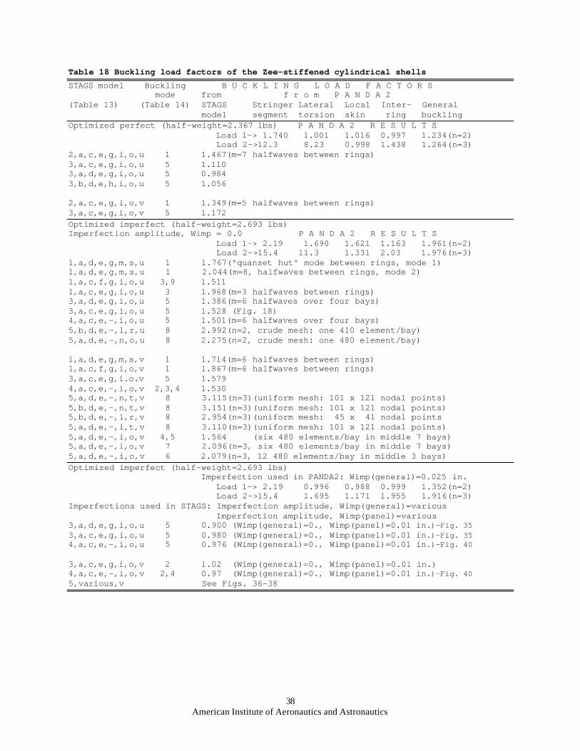
38American Institute of Aeronautics and Astronautics
Table 18 Buckling load factors of the Zee-stiffened cylindrical shellsSTAGS model Buckling B U C K L I N G L O A D F A C T O R S mode from f r o m P A N D A 2(Table 13) (Table 14) STAGS Stringer Lateral Local Inter- General model segment torsion skin ring bucklingOptimized perfect (half-weight=2.367 lbs) P A N D A 2 R E S U L T S Load 1-> 1.740 1.001 1.016 0.997 1.234(n=2) Load 2->12.3 8.23 0.998 1.438 1.264(n=3)2,a,c,e,g,i,o,u 1 1.467(m=7 halfwaves between rings)3,a,c,e,g,i,o,u 5 1.1103,a,d,e,g,i,o,u 5 0.9843,b,d,e,h,i,o,u 5 1.056
2,a,c,e,g,i,o,v 1 1.349(m=5 halfwaves between rings)3,a,c,e,g,i,o,v 5 1.172Optimized imperfect (half-weight=2.693 lbs)Imperfection amplitude, Wimp = 0.0 P A N D A 2 R E S U L T S Load 1-> 2.19 1.690 1.621 1.163 1.961(n=2) Load 2->15.4 11.3 1.331 2.03 1.976(n=3)1,a,d,e,g,m,s,u 1 1.767("quanset hut" mode between rings, mode 1)1,a,d,e,g,m,s,u 1 2.044(m=8, halfwaves between rings, mode 2)1,a,c,f,g,i,o,u 3,9 1.5111,a,c,e,g,i,o,u 3 1.968(m=3 halfwaves between rings)3,a,d,e,g,i,o,u 5 1.386(m=6 halfwaves over four bays)3,a,c,e,g,i,o,u 5 1.528 (Fig. 18)4,a,c,e,-,i,o,u 5 1.501(m=6 halfwaves over four bays)5,b,d,e,-,l,r,u 8 2.992(n=2, crude mesh: one 410 element/bay)5,a,d,e,-,n,o,u 8 2.275(n=2, crude mesh: one 480 element/bay)
1,a,d,e,g,m,s,v 1 1.714(m=6 halfwaves between rings)1,a,c,f,g,i,o,v 1 1.867(m=6 halfwaves between rings)3,a,c,e,g,i.o.v 5 1.5794,a,c,e,-,i,o,v 2,3,4 1.5305,a,d,e,-,n,t,v 8 3.115(n=3)(uniform mesh: 101 x 121 nodal points)5,b,d,e,-,n,t,v 8 3.151(n=3)(uniform mesh: 101 x 121 nodal points)5,b,d,e,-,l,r,v 8 2.954(n=3)(uniform mesh: 45 x 41 nodal points5,a,d,e,-,i,t,v 8 3.110(n=3)(uniform mesh: 101 x 121 nodal points)5,a,d,e,-,i,o,v 4,5 1.564 (six 480 elements/bay in middle 7 bays)5,a,d,e,-,i,o,v 7 2.096(n=3, six 480 elements/bay in middle 7 bays)5,a,d,e,-,i,o,v 6 2.079(n=3, 12 480 elements/bay in middle 3 bays)Optimized imperfect (half-weight=2.693 lbs) Imperfection used in PANDA2: Wimp(general)=0.025 in. Load 1-> 2.19 0.996 0.988 0.999 1.352(n=2) Load 2->15.4 1.695 1.171 1.955 1.916(n=3)Imperfections used in STAGS: Imperfection amplitude, Wimp(general)=various Imperfection amplitude, Wimp(panel)=various3,a,d,e,g,i,o,u 5 0.900 (Wimp(general)=0., Wimp(panel)=0.01 in.)-Fig. 353,a,c,e,g,i,o,u 5 0.980 (Wimp(general)=0., Wimp(panel)=0.01 in.)-Fig. 354,a,c,e,-,i,o,u 5 0.976 (Wimp(general)=0., Wimp(panel)=0.01 in.)-Fig. 40
3,a,c,e,g,i,o,v 2 1.02 (Wimp(general)=0., Wimp(panel)=0.01 in.)4,a,c,e,-,i,o,v 2,4 0.97 (Wimp(general)=0., Wimp(panel)=0.01 in.)-Fig. 405,various,v See Figs. 36-38
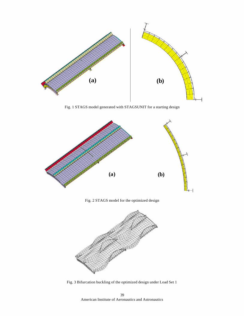
39American Institute of Aeronautics and Astronautics
Fig. 1 STAGS model generated with STAGSUNIT for a starting design
Fig. 2 STAGS model for the optimized design
Fig. 3 Bifurcation buckling of the optimized design under Load Set 1
(a) (b)
(a) (b)
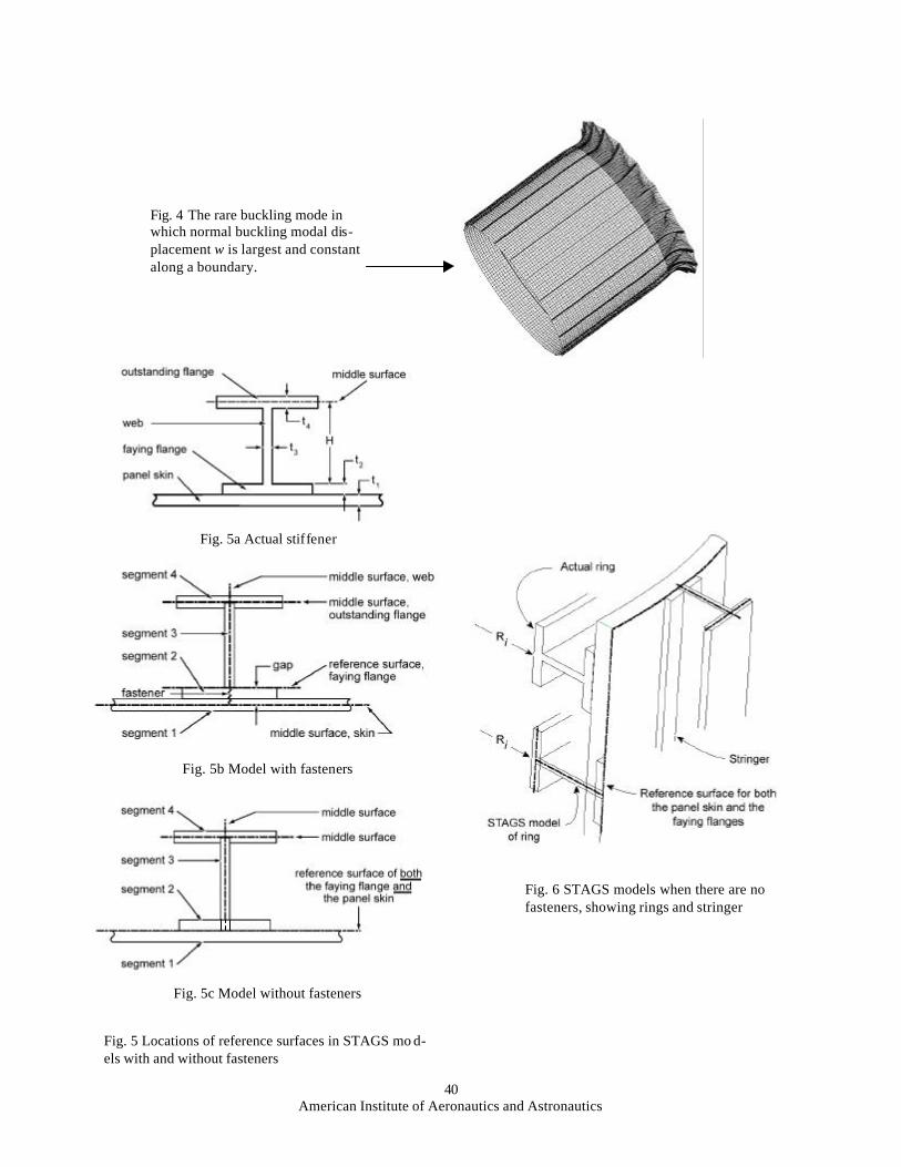
40American Institute of Aeronautics and Astronautics
Fig. 4 The rare buckling mode inwhich normal buckling modal dis-placement w is largest and constantalong a boundary.
Fig. 5 Locations of reference surfaces in STAGS mo d-els with and without fasteners
Fig. 6 STAGS models when there are nofasteners, showing rings and stringer
Fig. 5a Actual stiffener
Fig. 5b Model with fasteners
Fig. 5c Model without fasteners
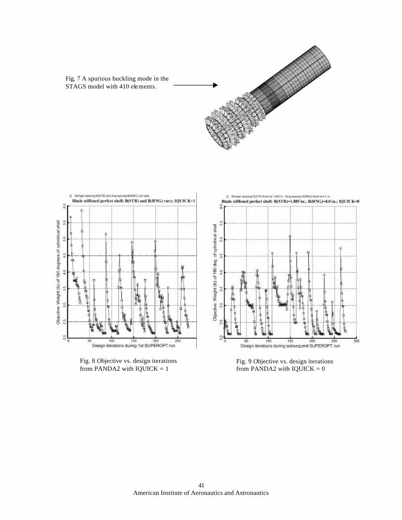
41American Institute of Aeronautics and Astronautics
Fig. 7 A spurious buckling mode in theSTAGS model with 410 elements.
Fig. 8 Objective vs. design iterationsfrom PANDA2 with IQUICK = 1
Fig. 9 Objective vs. design iterationsfrom PANDA2 with IQUICK = 0
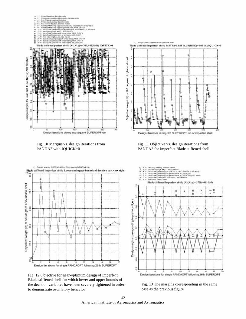
42American Institute of Aeronautics and Astronautics
Fig. 10 Margins vs. design iterations fromPANDA2 with IQUICK=0
Fig. 11 Objective vs. design iterations fromPANDA2 for imperfect Blade stiffened shell
Fig. 12 Objective for near-optimum design of imperfectBlade stiffened shell for which lower and upper bounds ofthe decision variables have been severely tightened in orderto demonstrate oscillatory behavior
Fig. 13 The margins corresponding in the samecase as the previous figure

43American Institute of Aeronautics and Astronautics
Fig. 14 Margins from design sensitivity run withPANDA2 for the optimized imperfect Bladestiffened shell
Fig. 15 Load-interaction curves for theoptimized imperfect Blade stiffenedshell analyzed both as if it were perfectand including the general buckling mo-dal imperfection with amplitudeWimp (general) = 0.025 in.
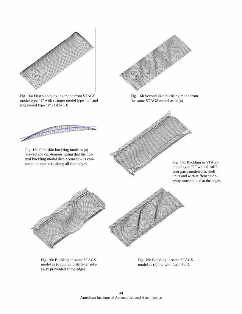
44American Institute of Aeronautics and Astronautics
Fig. 16a First skin buckling mode from STAGSmodel type “1” with stringer model type “m” andring model type “s” (Table 13)
Fig. 16b Second skin buckling mode fromthe same STAGS model as in (a)
Fig. 16c First skin buckling mode in (a)viewed end on, demonstrating that the nor-mal buckling modal displacement w is con-stant and non-zero along all four edges Fig. 16d Buckling in STAGS
model type “1” with all stiff-ener parts modeled as shellunits and with stiffener side-sway unrestrained at the edges
Fig. 16e Buckling in same STAGSmodel as (d) but with stiffener side-sway prevented at the edges
Fig. 16e Buckling in same STAGSmodel as (e) but with Load Set 2
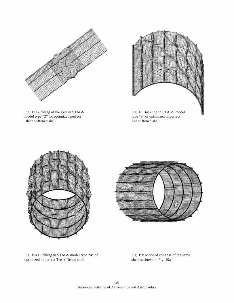
45American Institute of Aeronautics and Astronautics
Fig. 17 Buckling of the skin in STAGSmodel type “2” for optimized perfectBlade stiffened shell
Fig. 18 Buckling in STAGS modeltype “3” of optimized imperfectZee stiffened shell
Fig. 19a Buckling in STAGS model type “4” ofoptimized imperfect Tee stiffened shell
Fig. 19b Mode of collapse of the sameshell as shown in Fig. 19a
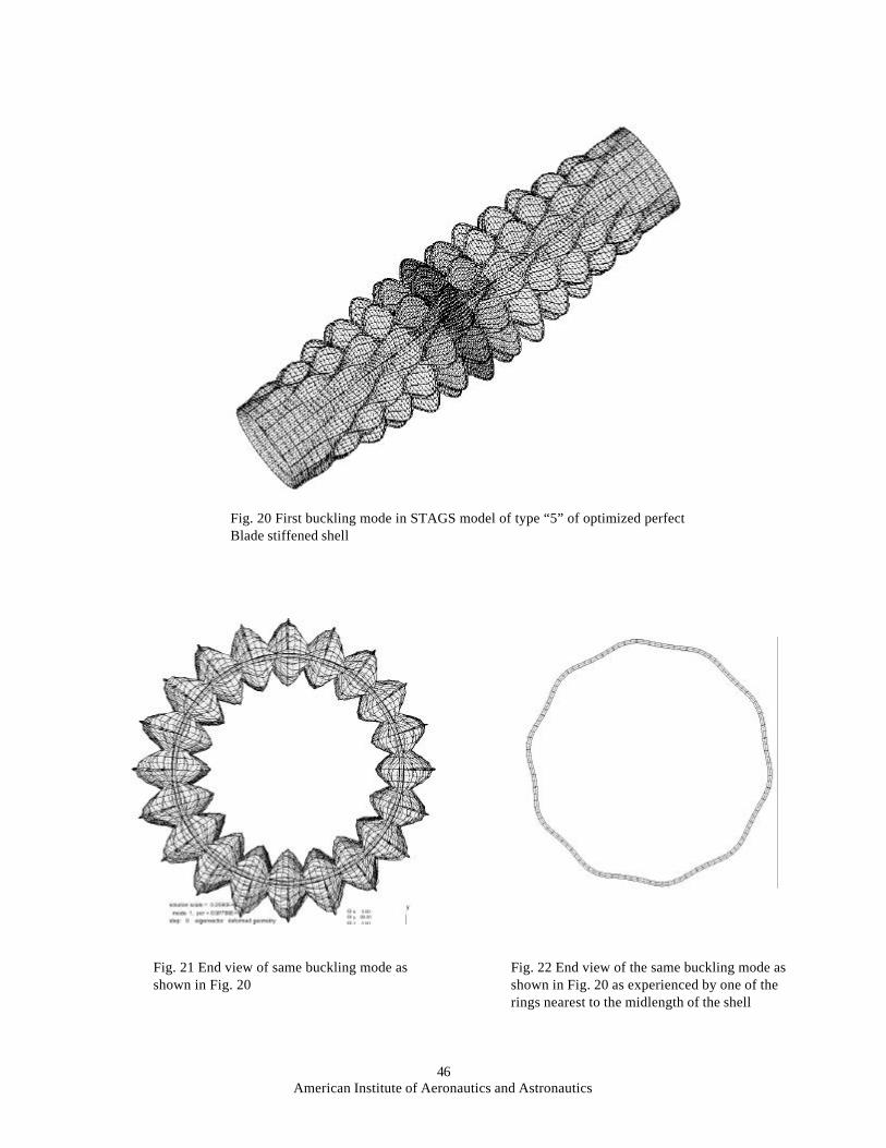
46American Institute of Aeronautics and Astronautics
Fig. 20 First buckling mode in STAGS model of type “5” of optimized perfectBlade stiffened shell
Fig. 21 End view of same buckling mode asshown in Fig. 20
Fig. 22 End view of the same buckling mode asshown in Fig. 20 as experienced by one of therings nearest to the midlength of the shell
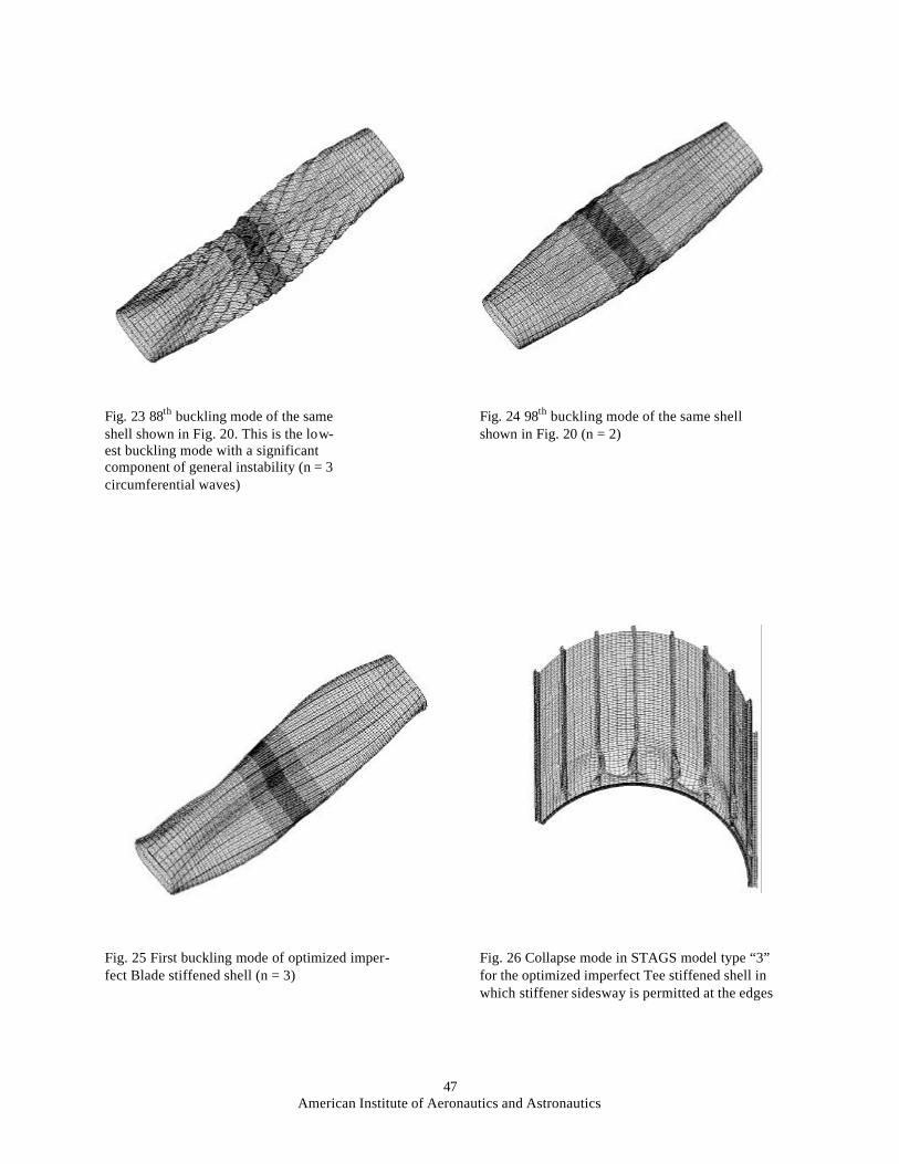
47American Institute of Aeronautics and Astronautics
Fig. 23 88th buckling mode of the sameshell shown in Fig. 20. This is the low-est buckling mode with a significantcomponent of general instability (n = 3circumferential waves)
Fig. 24 98th buckling mode of the same shellshown in Fig. 20 (n = 2)
Fig. 25 First buckling mode of optimized imper-fect Blade stiffened shell (n = 3)
Fig. 26 Collapse mode in STAGS model type “3”for the optimized imperfect Tee stiffened shell inwhich stiffener sidesway is permitted at the edges
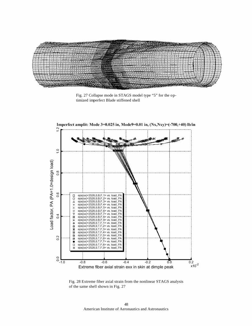
48American Institute of Aeronautics and Astronautics
Fig. 27 Collapse mode in STAGS model type “5” for the op-timized imperfect Blade stiffened shell
Fig. 28 Extreme fiber axial strain from the nonlinear STAGS analysisof the same shell shown in Fig. 27
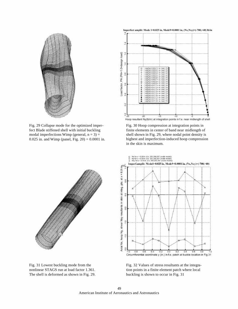
49American Institute of Aeronautics and Astronautics
Fig. 29 Collapse mode for the optimized imper-fect Blade stiffened shell with initial bucklingmodal imperfections Wimp (general, n = 3) =0.025 in. and Wimp (panel, Fig. 20) = 0.0001 in.
Fig. 30 Hoop compression at integration points infinite elements in center of band near midlength ofshell shown in Fig. 29, where nodal point density ishighest and imperfection-induced hoop compressionin the skin is maximum.
Fig. 31 Lowest buckling mode from thenonlinear STAGS run at load factor 1.361.The shell is deformed as shown in Fig. 29.
Fig. 32 Values of stress resultants at the integra-tion points in a finite element patch where localbuckling is shown to occur in Fig. 31
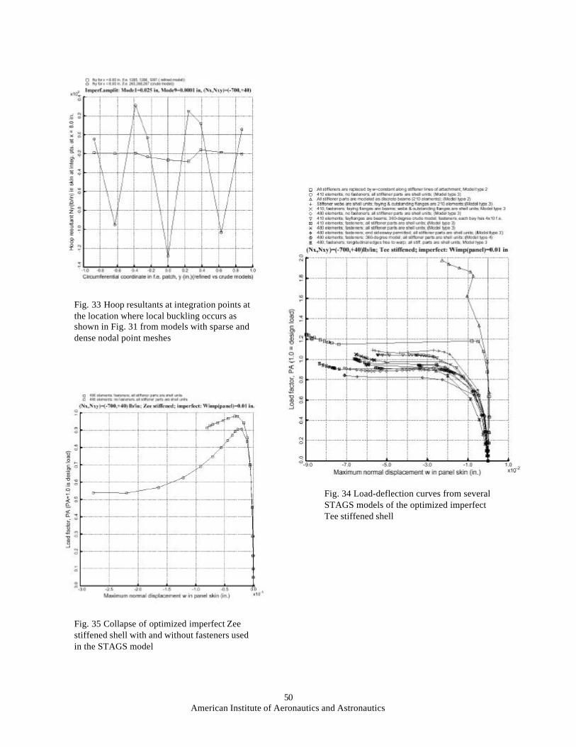
50American Institute of Aeronautics and Astronautics
Fig. 33 Hoop resultants at integration points atthe location where local buckling occurs asshown in Fig. 31 from models with sparse anddense nodal point meshes
Fig. 34 Load-deflection curves from severalSTAGS models of the optimized imperfectTee stiffened shell
Fig. 35 Collapse of optimized imperfect Zeestiffened shell with and without fasteners usedin the STAGS model
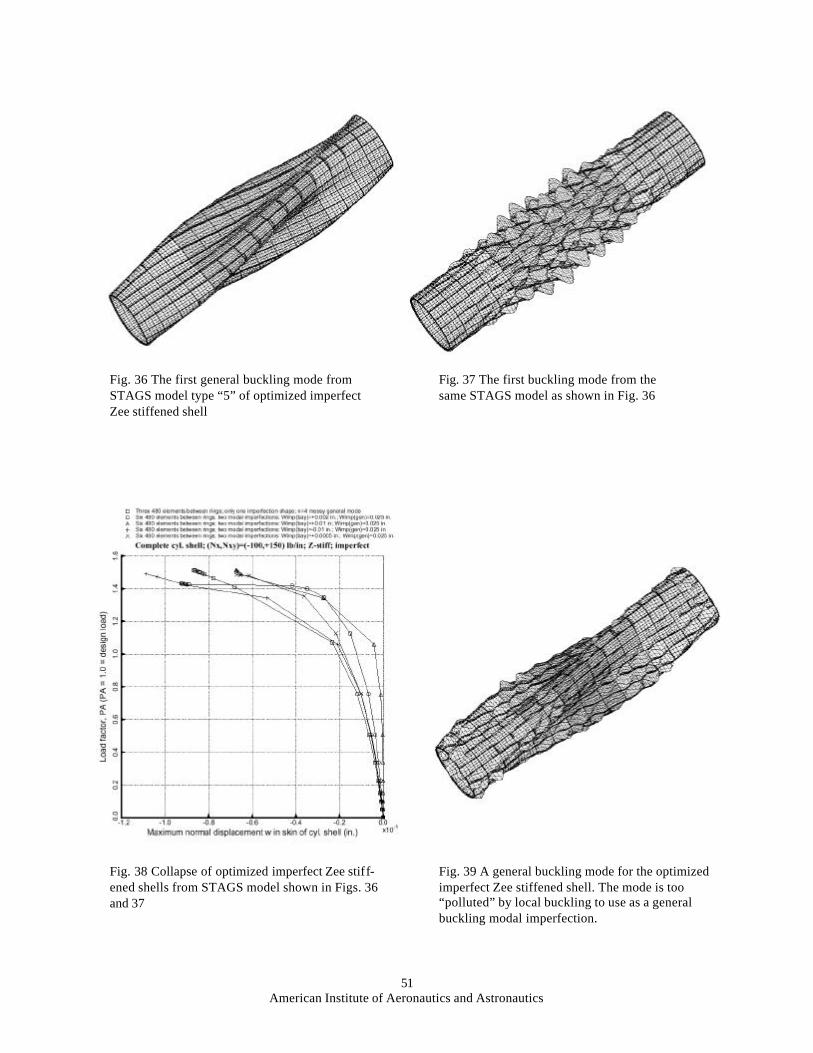
51American Institute of Aeronautics and Astronautics
Fig. 36 The first general buckling mode fromSTAGS model type “5” of optimized imperfectZee stiffened shell
Fig. 37 The first buckling mode from thesame STAGS model as shown in Fig. 36
Fig. 38 Collapse of optimized imperfect Zee stiff-ened shells from STAGS model shown in Figs. 36and 37
Fig. 39 A general buckling mode for the optimizedimperfect Zee stiffened shell. The mode is too“polluted” by local buckling to use as a generalbuckling modal imperfection.
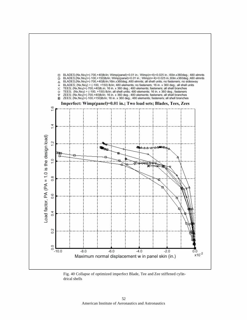
52American Institute of Aeronautics and Astronautics
Fig. 40 Collapse of optimized imperfect Blade, Tee and Zee stiffened cylin-drical shells