1

AIAA-2006-1751

Application of Linear Finite Elements to Finite Strain Using Corotation

Charles Rankin∗, Associate Fellow, AIAA Rhombus Consultants Group, Inc.

Suite B100, 1121 San Antonio Rd., Palo Alto, CA 94303 crankin@rhombuscgi.com

ABSTRACT Corotation methods have had great success in extending off-the-shelf element kernels to handle seamlessly large-deflection, large-rotation response with the limitation that strains must remain moderate. Element-independent methods promote element reuse by separating necessary opera-tions that filter out rigid rotation and enforce element self-equilibrium from other, element-specific tasks. The current paper presents a method that preserves element independence while at the same time removing the limitation of moderate strains, based on polar decomposition of the deformation state at the element centroid. The paper will begin with a short review of the foun-dations of corotation, followed by a detailed derivation of the new method, with close attention to preserving element independence. The efficacy of the method will be demonstrated with sev-eral cases of hyperelastic response with huge strains. A comparison will be made between ele-ments with linear strain-displacement kernels and Green’s strain, with almost identical results.

∗Consulting Specialist, Associate Fellow AIAA

2

Introduction As aerospace structures become lighter and more efficient, the possibility of nonlinear response increases, and indeed may present an advantage in their design. Consequently, analysis tools need to track all kinds of nonlinearity using finite elements and solution algorithms that are accu-rate and at the same time as efficient as possible. Element-independent corotation [1-3] has made great strides in turning shell or solid finite elements based on a simple linear strain-displacement formulation into ones capable of small-strain, large displacement response. If consistently ap-plied, this means proper treatment of geometric nonlinearity, including the generation of the “geometric” stiffness needed to assure convergence in a nonlinear analysis, or for a buckling ei-genanalysis. In this paper, we wish to build on the work of Moita and Crisfield [4-5] to demon-strate that corotation can be applied to problems with an elastic potential, and thereby remove the restriction to small strains. Derivations will be followed by examples of the response of a Mooney-Rivlin material undergoing large strains, all using shell elements with a linear strain-displacement formulation.

Limitations of Standard Corotational Implementations The motivation for this paper is the discovery that standard implementations of corotation [1-3,7] do not account for sufficient rigid-body motion as the deformation becomes large. This realiza-tion has generated a number of important papers [4-10], including [4-5] mentioned above. In contrast, standard corotation has had an excellent track record for problems with arbitrary dis-placements (very large, including structures with parts that undergo many complete rotations) for moderate strain response. Work in [1-3] has shown how to correct for element defects to insure self-equilibrium of forces generated from a strain energy field for large displacement response. A product of this effort is a procedure for producing corrected internal forces and a consistent stiff-ness matrix given only the displacement field, the element rotation, and the usual element kernel outputs. As the strain becomes large, however, standard methods yield a rotation of the material reference frame (expressed as an orthogonal transformation) that deviates from irrotational de-formation characteristic of the pure stretch determined by polar decomposition. This is demon-strated by the presence of a finite rotation of the corotational frame even for a displacement field representing a pure deformation. The good news is that for so-called element-independent meth-ods, very little software needs to be modified if, as we shall show, only that part of the computa-tion that concerns the transformation itself and its first variation is affected. The focus of this pa-per is to demonstrate that almost all the development in [1-3] can be applied without significant alteration to an “irrotational” choice of element frame that insures a pure deformation field at the element centroid. Therefore, standard element-independent corotation can be extended with a minimum of effort to large strain deformation.

A Review of Element-Independent Corotation Most of what is covered in this section is taken from [1-3], where the reader will find a complete derivation of the theory in great detail. A brief summary here, however, will clarify the basic steps in corotation and lay the groundwork for developments in this paper. The fundamental idea is to find a transformation that operates on the global displacements and in the process re-

3

moves the rigid-body contribution before the finite element kernels use them. This kind of “fil-ter” is permitted because for strain energy applications, rigid body motion does not contribute to the energy. This fact is succinctly expressed in the polar decomposition theorem, which states that the deformation in the structure can be partitioned into a pure deformation devoid of rotation followed by a pure rotation:

RUF = (1)

where F is the deformation gradient, R is a pure rotation, and U is the right stretch tensor repre-senting a deformation without rotation. Whereas (1) represents a tensor relationship that varies from point to point, all forms of corotation attempt to provide an approximate rotation TG that is a close analogue to R in an average sense over a given element. Clearly, in the limit of a fine grid, if TG is a good approximation for some point in the element, then the effects of rigid-body motion can be ignored for the whole element. Element-independent methods strive to separate cleanly corotation from element kernels, so that at most there is a “filter” that processes incom-ing displacements, and filters that correct resulting “native” internal force vectors and stiffness matrices after the local element operations are complete. Operations structured in this manner greatly simplify both development of and use of finite element software, and promote element reuse. Perhaps the best treatise on the subject is by Felippa [10], where the subject of corotation is also covered in detail. Element reuse is one of the primary motivations for the work that fol-lows. In this short summary, we shall concentrate on the translational displacements, and only briefly state results that include nodal rotations where applicable. For those interested in how corotation deals with nodal rotations, we again refer to [1-3]; our work here will not affect how they are handled in any way. The fundamental relationships in corotation are as follows:

( )( )

ieii

iii

iT

ei

eiiTGi

uXxuXx

XXTX

XxxTu

+=+=

−=

−−=

00

0

(2)

Here we have TG that is an orthogonal transformation that removes (most) of the rigid-body mo-tion, and T0 that is an initial transformation that can be chosen arbitrarily for convenience.

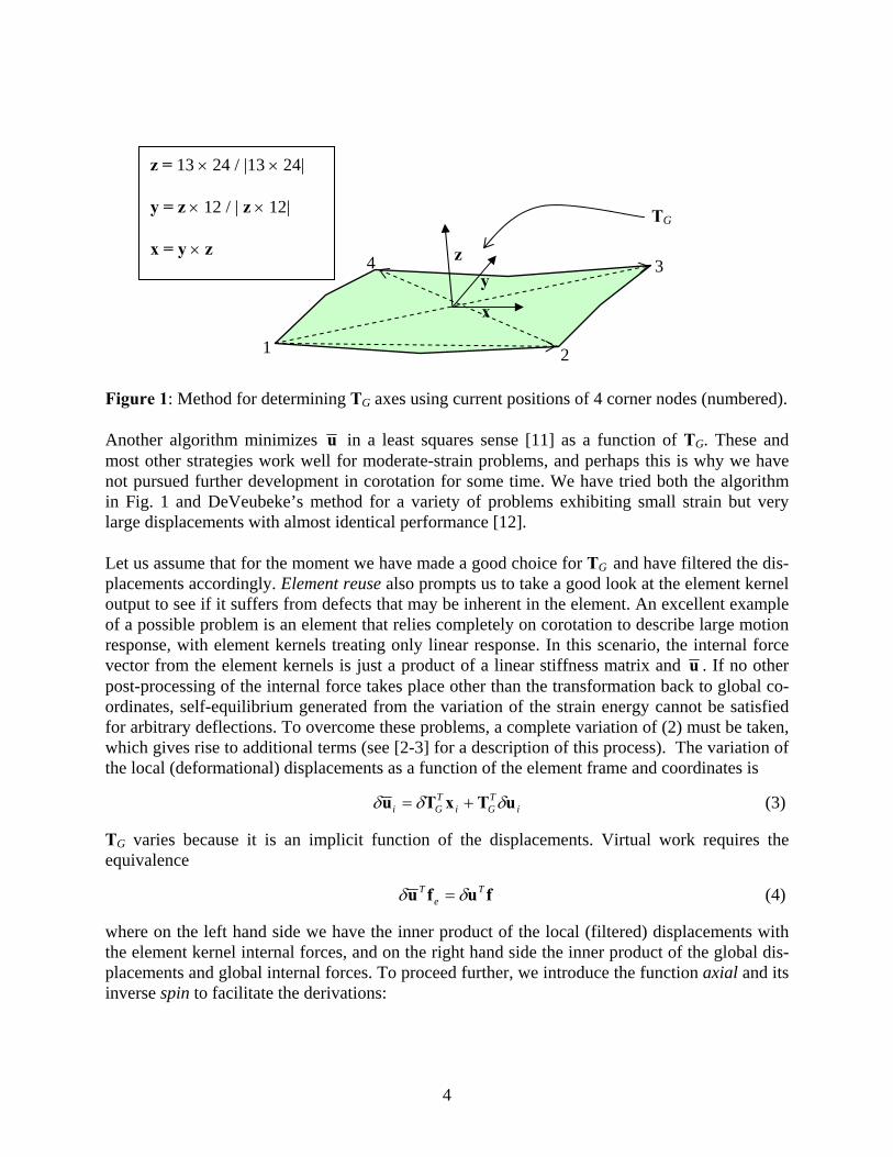
iX and 0X are the initial (undeformed) coordinates for a given node i and the origin, respec-tively, whereas ix and 0x are the current (deformed) coordinates; in the development that fol-lows we will drop reference to the origin, which can be arbitrary and does not effect our compu-tations, provided element kernels are not sensitive to translations (translation-sensitive elements are extremely uncommon). u are the displacements after the “filter,” and ideally represent as closely as possible a pure deformation. What makes this procedure work of course is a good choice for TG, and most of the literature on corotation concerns this choice either directly or in-directly. One of the more common methods for determining TG is to compute a normal from the cross product of diagonals constructed from selected corner nodes, and to align one of its axes as closely as possible along a line between two nodes as shown in Fig. 1.

4

Figure 1: Method for determining TG axes using current positions of 4 corner nodes (numbered). Another algorithm minimizes u in a least squares sense [11] as a function of TG. These and most other strategies work well for moderate-strain problems, and perhaps this is why we have not pursued further development in corotation for some time. We have tried both the algorithm in Fig. 1 and DeVeubeke’s method for a variety of problems exhibiting small strain but very large displacements with almost identical performance [12]. Let us assume that for the moment we have made a good choice for TG and have filtered the dis-placements accordingly. Element reuse also prompts us to take a good look at the element kernel output to see if it suffers from defects that may be inherent in the element. An excellent example of a possible problem is an element that relies completely on corotation to describe large motion response, with element kernels treating only linear response. In this scenario, the internal force vector from the element kernels is just a product of a linear stiffness matrix and u . If no other post-processing of the internal force takes place other than the transformation back to global co-ordinates, self-equilibrium generated from the variation of the strain energy cannot be satisfied for arbitrary deflections. To overcome these problems, a complete variation of (2) must be taken, which gives rise to additional terms (see [2-3] for a description of this process). The variation of the local (deformational) displacements as a function of the element frame and coordinates is

iTGi

TGi uTxTu δδδ += (3)

TG varies because it is an implicit function of the displacements. Virtual work requires the equivalence

fufu Te

T δδ = (4)

where on the left hand side we have the inner product of the local (filtered) displacements with the element kernel internal forces, and on the right hand side the inner product of the global dis-placements and global internal forces. To proceed further, we introduce the function axial and its inverse spin to facilitate the derivations:

1 2

3 4 z

x

y

z = 13 × 24 / |13 × 24| y = z × 12 / | z × 12| x = y × z

TG

5

( )

( )⎥⎥⎥

⎦

⎤

⎢⎢⎢

⎣

⎡

−−

−≡

⎟⎟⎟⎟

⎠

⎞

⎜⎜⎜⎜

⎝

⎛

⎥⎥⎥

⎦

⎤

⎢⎢⎢

⎣

⎡

−−

−=

⎟⎠⎞

⎜⎝⎛ −≡=

00

0spin

00

0axial

][21axialaxial

xy

xz

yz

xy

xz

yz

T

vvvv

vv

vvvv

vv

v

VVVv

(5)

Equation (5) is just a statement of the relationship between an axial vector and an antisymmetric matrix. It is elementary to demonstrate that (3) can be converted to a much more useful form as follows:

( )( )

( ) ( ) ( )

( ) GTGe

jj

j

eieiie

iTGGg

TG

igTGi

TG

TTω

uuω

xωxxω

xTTωT

xωTxT

δδ

δδδ

δ

δδ

=

∂∂

==−=

−=

−=

∑

spin

spinspinspin

spin

spin

(6)

Here, gωδ and eωδ are variations of the instantaneous rotation expressed in the global and ele-ment frames, respectively. The last term in the third equation of (6) is valid because the element frame depends only on the nodal displacements, and G

TG TT δ is antisymmetric because of the or-

thogonality of TG. If we combine (6), (3), and (4) together, we have the important relationship

( )( )( )( )

( ) uTPu

fPf

fTffPTu

fΓΦITu

fufu

δδ

δ

δ

δδ

TG

eT

c

cG

eT

GT

eT

GT

Te

T

diag

diagdiag

diag

=

≡

=∴=

−=

=

(7)

The matrix ( )GTdiag is 3N by 3N matrix of zeros except for TG arranged repeatedly along the main diagonal with one 3x3 block for each of N nodes. From (6), the matrix TΦ is

( ) ( ) ( )[ ]NiT xxxΦ spinspinspin 1≡ (8)

which when extended to elements with nodal rotational freedoms (from [2-3]) becomes

( ) ( ) ( )[ ]3331 spinspinspin IxIxIxΦ NiT ≡ (9)

6

The derivation in (9) from (8) is straightforward and is not included here. The other new quantity Γ is defined as

⎥⎦

⎤⎢⎣

⎡∂∂

∂∂

∂∂

≡ 3331

0uω

0uω

0uω

ΓN

e

i

eeT (10)

Each of the derivative quantities is arranged to correspond to the sum in (6). For convenience, we have expressed the displacements in the local element frame, which can be computed from the global coordinates by applying (2) and realizing that the undeformed local coordinates are constants. From the structure of (7) we see that the action of P is in fact a “filter” because the product e

T fΦ is the expression for nodal self-equilibrium:

( )( )

( ) fi

ieii

iieiie

T

mmfx

mfxfΦ

=+×=

+=

∑

∑ spin (11)

Here, we have included rotations for completeness. Clearly, if the element adheres strictly to self-equilibrium with respect to the updated coordinates, (11) evaluates to zero, so that the only remaining term in (7) is the ordinary transformation of the local forces to the global frame. fm is therefore a moment that represents the error in the element kernel formulation, a term that will be used frequently in what follows. It is clear that if our “corrected” force cf is to satisfy equilib-rium, then

( ) 0=−= eTT

cT fΓΦIΦfΦ (12)

which in turn requires that the bi-orthogonality relationship

3IΓΦΦΓ == TT (13)

be satisfied. If (13) is true, then P is a projector (idempotent), so that

PΦΓIΦΓΦΓΦΓIP =−=+−= TTTT22 (14)

(13) has been shown to be satisfied for all the standard element frames found in [1-3], and for the least squares method in [11]. We shall have to demonstrate (13) for our new choice of element frame.

“Irrotational” Corotation The polar decomposition

To extend corotation to large deformation analysis, we consider the work of Moita [4-5] and at-tempt to base the selection of TG on polar decomposition. We are faced with two limitations that must be dealt with in the beginning if we are to preserve element independence and promote element reuse. First, as we have covered above, polar decomposition cannot be satisfied over the whole element using corotation alone; in order to allow variation within an element, one must implement polar decomposition as part of the local strain computations, and not through corota-tion. However, as the mesh become increasingly refined, what is satisfied at the element centroid

7

becomes increasingly valid throughout. This is the same limitation for corotation in a small-strain setting, so we do not consider it a problem for large deformation problems either. The sec-ond limitation is that in order to compute the displacement derivatives at the centroid, one re-quires some sort of “shape functions” to interpolate nodal displacements. At first glance, it would appear that one would have to have access to element details to provide these functions, thereby losing the advantage of element independence. Fortunately, since a very small set of al-ternate shape functions serves perfectly well as interpolators for almost any element connec-tivity, we can easily maintain element independence and maximize element reuse. The first step required to compute polar decomposition at the centroid is to calculate the defor-mation gradient F. A succinct expression for this is the following:

( )

[ ]

[ ]Nl

Nl

Nl

Nl

NlT

zzz

yyy

xxxT

i

Tii

TTi

Tiie

T

wwwvvvuuu

wvuwvuwvu

vvvB

uuud

G

xvGIF

uvdXBG

1

1

1

1

1

,,,

,,,

,,,

≡

=⎥⎥⎥

⎦

⎤

⎢⎢⎢

⎣

⎡=

⎥⎥⎥

⎦

⎤

⎢⎢⎢

⎣

⎡=

=+=

==

∑

∑

(15)

G is the displacement gradient, d is a nodal displacement matrix with the deformational dis-placements arranged as one column for each node, and B is a matrix that depends on the choice of alternate shape functions and the initial geometry only (see Moita [4,6], where he uses the symbol a instead of v). The only assumptions here are that the shape function derivatives are not singular at the centroid for any possible nodal configuration, and that interpolation of the dis-placements is independent of component direction (isoparametric). It can be shown rather easily that for interpolation to the centroid, any arrangement of nodes that provides a positive element area or volume will not be singular, and that it is always possible to use isoparametric alternate shape functions even for complex elements. The important thing here is to remember that the vectors v are independent of the displacements. The next step is to compute the polar decomposition and extract the rotation R. A standard method for doing this is to solve the eigenproblem for FFT to determine the stretch, and then to back out R. Instead, we propose an alternate method because as a byproduct, it yields also an explicit expression for Γ defined in (10). Equation (1) can be recast as

TRT

TFU=

= (16)

8

with the idea to compute T directly using Newton iteration. Our requirement is that U be sym-metric for all changes to T that preserve its orthogonality. Since the rotation T is the only un-known quantity, the variation of U is the same as the product of the variation of T times F:

TFU δδ = (17)

We also have

UUTT

)spin()spin(

ωδωδ

=∴=

(18)

We can show that

( ) [ ]δωδ UUIU −=− )trace()axial(2 3 (19)

by expanding the expressions out long hand and comparing term-by-term. Only the symmetric part of the operator on the right hand side of (19) needs to be used, since upon convergence and satisfaction of

0)axial(2 =U (20)

U and the operator H are symmetric and positive definite. With these facts established, it is not difficult to demonstrate that the sequence

[ ] ( )

[ ]{ } { }ii

s

TUUωT

UωUHωUUI

∆←

=∆

−=≡−

+1

)spin(exp)axial(2)trace(

δδδ

(21)

has the desired quadratic convergence properties. Here, the subscript s reminds us that the sym-metric part of the matrix is used in the solution of the 3x3 system for δω . The superscript in the curly brackets is an iteration counter; experience has shown that convergence is obtained to ma-chine precision in less than 5 iterations, worst case. Initial estimates for T can be obtained from any “standard” corotation method. If T has been computed using displacements expressed in the initial local element frame T0, TG is easily shown to be

RTTTT 00 == TG (22)

Equation (22) states that TG represents a rotation first of the structure defined by polar decompo-sition at the centroid, followed by an initial rotation T0 that is chosen for convenience and is con-stant throughout the analysis. If the initial rotation is unity, TG is identical to the rotation deter-mined from polar decomposition; if the displacement field is a pure deformation, TG reduces to T0, as expected. It is also straightforward to show that displacements computed using (2) and (22) yield a deformation gradient that is a pure stretch and therefore symmetric at the element centroid, and that strains are referred to system T0 in exactly the same manner as was done pre-viously in standard corotation. The actual computations follow easily from (21) and (15). From (15) we have

9

( ) ( ) ( )

( )

( )∑

∑

∑

=

=

=

=

⎟⎠

⎞⎜⎝

⎛×=

⎟⎠

⎞⎜⎝

⎛−=

==

N

ll

N

lll

N

l

Tll

Tll

1l

1

1

spin

spinaxial

axial

axial 2axial2axial 2

uv

uv

uvvu

GFU

(23)

The operator H becomes

( )∑=

−⋅=−=N

l

Tllll

133 )( trace vxxvIFFIH (24)

Finally, from (23) and the last of (6) we see that

( )FωHωω

δδδδ

axial2=−=

e

e (25)

The Variation of the Element Frame

From (25) we can see immediately how to compute Γ:

( )

( ) ( ) ( )[ ]uΓωBHΓ

vvvBuB

FωH

δδ

δδδ

TeS

TNlS

S

e

==∴

≡==

− because

spinspinspin

axial2

11

(26)

where u without subscripts represents a column vector of nodal displacements 3N long. Equa-tion (26) forms the basis for establishing the bi-orthogonality relationship (13) and for develop-ing a consistent tangent stiffness matrix. Proof of the Bi-Orthogonality Condition

To prove (13) we write out the relationship

( ) ( )

( )

3

31

1 spinspin

I

vxxvIH

xvHΦΓ

=

−⋅=

−=

∑

∑−

−

i

Tiiii

iii

T

(27)

In this derivation we used the identity

( ) ( ) baIbaba ⋅−= 3spinspin T (28)

10

Equation (28) can be verified term-by-term. Benefits of Extended Corotation

We have demonstrated that corotation based on an element frame TG computed using polar de-composition yields a pure deformation at the element centroid. Moreover, it can be shown [6] that strain computed from a small-strain approximation approaches U – I, or Biot strain in the limit of a fine grid. We also have proved that the projector P has the required properties to act as a filter that enforces self-equilibrium on the internal forces computed by element kernels, as re-quired by rotational invariance. Biot strain serves as an excellent starting point for a large strain analysis, even when only linear strain-displacement relationships are implemented in the element kernels. A summary of obvious benefits of extended corotation include

1. In the limit of a fine grid, a pure deformation state is guaranteed within each element. 2. The rotation of the element frame is independent of node numbering and order, choice of

origin, and initial element frame. 3. The projector properties required to enforce self-equilibrium are preserved. 4. Implementation presents no additional difficulties when compared to standard corotation. 5. Element independence and reuse are preserved. 6. The development of extended corotation provides insight into how corotation works.

In the next section, we shall demonstrate that additional properties of P are preserved that greatly simplify the computation of a consistent tangent stiffness matrix, and that no assumptions about the kernel internal force vector need to be made. The Consistent Tangent Stiffness Matrix

In the literature, justification for omitting the derivative of Γ when computing the tangent stiff-ness matrix is based on the satisfaction of local equilibrium within each element. For internal forces derived from the strain energy, this must be true, but as we have shown above, many ele-ments suffer from defects that produce an out-of-balance moment fm . It is precisely for this reason that the authors in [3] took great pains to insure that all derivatives and the resulting “geo-metric” stiffness depend only on “corrected” internal forces cf that had first been passed through the corotational projector P, Equation (7). Although not repeated here, the authors in [3] have shown that if

TTT ΦΓΓΓ δδ −= (29)

then the remainder of the arguments in [3] remain valid, and corotation applied using these methods remains virtually element independent, again promoting element reuse. An additional benefit is that almost no corotational software already developed has to be changed, except for the kernel that computes the updated element frame TG and its derivative Γ. Our goal is to prove (29). The first step is to derive the variation of Γ from its definition in (26). The total quantity to be varied for the tangent stiffness is

11

( )( )

TTf

TTe

Te

TTTe

Te

Te

Te

Te

ΓmΦΓfPf

ΓΦΦΓfPf

PfPfPf

δδδ

δδδ

δδδ

−−=

+−=

+=

(30)

Only the last term in (30) concerns us here because it is the only one that depends on the deriva-tive of Γ. This last term varies as

( ) STf

TTf BHmΓm 1−−=− δδ (31)

because only H depends on the element nodal displacements. We use the following

111 −−− −= HHHH δδ (32)

to establish

f

Tf

TTf

TTf

TTf

mHz

HΓzHΓHmΓm−

−

≡

==− δδδ 1

(33)

If we use the definition of H from (24), we obtain the following variation after minor rearrange-ment:

( ) ( ) TN

lfl

Tlll

Tf

TTf ΓzxvvxzHΓz ⎥

⎦

⎤⎢⎣

⎡⋅−⋅= ∑

=1δδδ (34)

Now let us compare that result with (29):

( )[ ] ( ) Tll

Tf

TS

Tf

TS

Tf

TTTf

TTf

Γxvz

ΦΓBz

ΦΓBHm

ΦΓΓmΓm

⎥⎥⎥

⎦

⎤

⎢⎢⎢

⎣

⎡−=

=

=

=−−

δ

δ

δ

δδ

spin spin

1

(35)

The matrix product in (35) yields

( )[ ] ( ) ( ) ( )

( ) ( ) TN

lfl

Tlll

Tf

Tl

N

ll

Tf

Tll

Tf

Γzxvvxz

ΓxvzΓxvz

⎥⎦

⎤⎢⎣

⎡⋅−⋅=

⎥⎦

⎤⎢⎣

⎡−=

⎥⎥⎥

⎦

⎤

⎢⎢⎢

⎣

⎡−

∑

∑

=

=

1

1spin spin spin spin

δδ

δδ (36)

We see that (34) and (36) are identical, proving our assertion.

12

We now shall show that permissible variations of the local “filtered” displacements preserve the symmetry of H and therefore F. The symmetry of H implies the following:

( )

( )∑

∑

=

=

×=

−=−

N

lll

N

l

Tll

Tll

T

1

1

spin vx

xvvxHH

δ

δδδ (37)

Hence it is sufficient to prove

0 11

=×=× ∑∑==

N

lll

N

lll xvvx δδ (38)

Starting from the last equation in (7), we proceed as follows:

( ) ( )

( )( )( ) uTu

uΓΦIv

uPvuvuv

δδ

δ

δδδ

TG

N

l

Tll

N

lll

N

lll

N

lll

diag ˆ

ˆspin

ˆspinspin

13

111

≡

−=

==×

∑

∑∑∑

=

===

(39)

where lP is the part of P that pertains to node l. We now use the definition of Φ and Γ to yield:

( ) ( ) ( ) ( ) ( )

( ) ( )[ ] ( )

0

ˆspin ˆspin

ˆspin spinspinˆspinspin

1

1

13

1

1

1

111

=

⎥⎦

⎤⎢⎣

⎡−⋅−=

⎥⎦

⎤⎢⎣

⎡−=

∑∑∑

∑∑∑∑

=

−

==

=

−

===

N

kkk

N

l

Tllll

N

lll

N

kkk

N

lll

N

lll

N

lll

uvHvxxvIuv

uvHxvuvuv

δδ

δδδ

(40)

Thus H and F remain symmetric for all permissible variations of the displacements. This is as it must be, since P must take into account any variation in the element frame required to enforce the irrotational constraint at the element centroid. Given (29), we have

TΦΓPP δδ −= (41)

so that the remainder of the arguments in [3] apply unchanged. The consistent tangent stiffness is (including rotations)

( ) ( )

( )[ ]( ) ( )[ ]cici

Tci

T

TTTet

TG

etG

gt

mfF

0fF

ΓFPFΓPKPK

TKTK

spinspin

spinˆ

ˆdiagdiag

3

−−≡

−≡

−−=

=

(42)

13

where cif and cim are the projected (“filtered”) forces and moments for node i. The quantity K is the element kernel stiffness matrix. Provided K is consistent with the kernel internal force vector, g

tK is a fully consistent tangent stiffness matrix expressed in global system coordinates, ready for assembly. Alternate Shape Functions

Because one of the primary objectives of corotation is element reuse, we seek a method that would apply to all elements of a given type that is sufficiently accurate to meet the irrotational criterion independent of the particular shape functions in a given element. Since we need infor-mation only at the element centroid, our task is greatly simplified, because no matter how nodes are arranged in the element, if it has finite volume (or area for shell or interface elements), the lowest possible interpolation order will suffice. Almost all cases are adequately covered by low-order Lagrange shape functions that interpolate a subset of element nodes. It is in fact not neces-sary that all element nodes participate, so long as the interpolation is well defined within the ele-ment. We were able satisfy our requirements for solid elements containing 4, 8, 20, and 27 nodes using only two basic sets of functions. All shell elements can be handled by using only the cor-ner nodes and the simplest bilinear interpolation. The computation of the vectors v used to de-termine our displacement gradient and derivatives is based on standard finite element methods that need not be covered here. Maintaining element independence is straightforward even when the kernels have unusual node numbering or when our alternate functions use either a super- or subset of element nodes. The latter case is the simplest since there will certainly be a subset of eight “corner nodes” (four for shell elements) that can be chosen and listed in an index array to be passed to corotational soft-ware. For elements with fewer nodes than required by our alternate functions, a similar strategy can be used, except that this time the index array will have one or more repeated indices. For example, a tetrahedral is handled nicely by passing an index array that looks like this:

[ ]34413221 (43)

and using the 8-node linear Lagrange functions for interpolation (it is interesting to note that the results from the 8-node functions and (43) are identical to those derived from tetrahedral shape functions). In this example, Γ is computed for eight nodes, but values are accumulated to the ac-tual node number in the index list before output. This method works because all quantities that multiply Γ are identical for repeated entries in the list (includes displacements, coordinates, stiff-ness matrix elements, and internal forces). This property insures that we achieve our goal of maximum element reuse. For elements with greater than the number nodes necessary for interpo-lation, Γ will be zero for any node not in the index list; we therefore continue to assume that Γ depends only on the selected set of interpolation nodes that are specified in the list. This prac-tice has been in use in corotation applications derived in [1-3] without difficulty since the begin-ning. Specialization for Shells

For shells, the deformation gradient for the mid-surface strains is

14

⎥⎥⎥

⎦

⎤

⎢⎢⎢

⎣

⎡

++

=

zyx

yyx

xyx

nwwnvvnuu

,,,

,,,

,,,

11

F (44)

where n is the unit normal to the surface. We shall assume that the bending strains are small compared to the membrane strains as membrane strains become large, in agreement with as-sumptions that underlie shell elements. We define TG as a product of two transformations

ETT =G (45)

where E is computed by any method that defines its z axis to be normal to the shell at its cen-troid; an example of an acceptable strategy is shown in Fig. 1. If the z axis coincides with the shell normal, we can show that the derivatives of the transverse displacement w, when expressed in system E, also vanish for any transformation T that leaves the normal unchanged. Therefore, it is straightforward to show that standard procedures are sufficient to determine not only the z axis, but also the first two rows of ΓT. We are left with the computation of the last row of ΓT, which is determined by a rotation about the local z axis that makes F symmetric. The only sur-viving off-diagonal terms in F are xv, and yu , , which must be equal. For this case, Eq. (21) has a closed form solution because T reduces to:

⎥⎥⎥

⎦

⎤

⎢⎢⎢

⎣

⎡ −=

1000cossin0sincos

θθθθ

T (46)

where

yx

xy

vuvu

,,

,,

2tan

++

−=θ (47)

Please also see the development in [13]. From the derivative of T, (26) becomes

( ) ( )

( )3,,

31

333

21

S

yx

ST

vuB

BHΓ

++=

= −

(48)

where ( )3• is the third row of the quantity indicated. Software Organization

At this point it is useful to show where existing corotational software requires modification. In the process, we shall see just how little additional work is required to implement irrotational corotation. The logical flow for the internal forces is

15

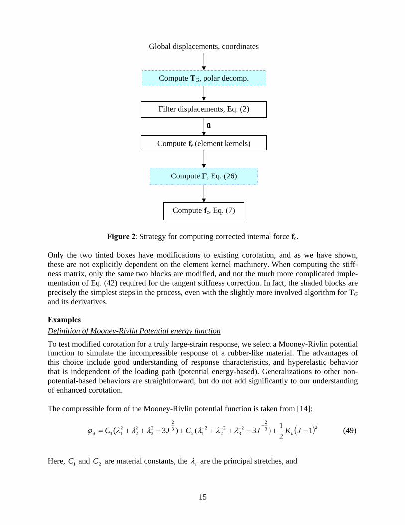
Figure 2: Strategy for computing corrected internal force fc. Only the two tinted boxes have modifications to existing corotation, and as we have shown, these are not explicitly dependent on the element kernel machinery. When computing the stiff-ness matrix, only the same two blocks are modified, and not the much more complicated imple-mentation of Eq. (42) required for the tangent stiffness correction. In fact, the shaded blocks are precisely the simplest steps in the process, even with the slightly more involved algorithm for TG and its derivatives.

Examples Definition of Mooney-Rivlin Potential energy function

To test modified corotation for a truly large-strain response, we select a Mooney-Rivlin potential function to simulate the incompressible response of a rubber-like material. The advantages of this choice include good understanding of response characteristics, and hyperelastic behavior that is independent of the loading path (potential energy-based). Generalizations to other non-potential-based behaviors are straightforward, but do not add significantly to our understanding of enhanced corotation. The compressible form of the Mooney-Rivlin potential function is taken from [14]:

( )232

23

22

212

32

23

22

211 1

21)3()3( −+−+++−++=

−−−− JKJCJC bd λλλλλλϕ (49)

Here, 1C and 2C are material constants, the iλ are the principal stretches, and

Compute TG, polar decomp.

Global displacements, coordinates

Filter displacements, Eq. (2)

Compute Γ, Eq. (26)

Compute fe (element kernels)

ū

Compute fc, Eq. (7)

16

change volume321 == λλλJ (50)

The bulk modulus bK for us either will be a large number (for solid elements, plane-strain shells), or will be ignored when constant volume is imposed as a constraint (plane-stress shell element response). For solid and plane-strain shell elements, we shall treat two cases:

1. Green’s strain, applicable equally to existing and enhanced corotation. 2. Biot’s strain, the limiting strain with enhanced corotation, fine mesh.

The conjugate second Piola Kirchhoff (PK2) stress is [14] related to the principal Green stretches

221 iii Ee λ=+= by

( ) ibiiiii eJJKeJeCeJCS /1212 132

22

132

1 −+⎟⎟⎠

⎞⎜⎜⎝

⎛−−⎟

⎟⎠

⎞⎜⎜⎝

⎛−= −−−− (51)

We shall not go into the details of (51) or explain how we derived the tangent modular matrix, but the steps are straightforward and taken almost verbatim from [14]. The stresses in (51) are in the principal strain coordinate system; transformation to local element coordinates is straight-forward. The conjugate Biot stress is related to the principal stretches B

ii E+= 1λ by

( ) ibiiiiBii JJKJCJCS λλλλλ /12 13

23

213

2

1 −+⎥⎥⎦

⎤

⎢⎢⎣

⎡⎟⎟⎠

⎞⎜⎜⎝

⎛−−⎟

⎟⎠

⎞⎜⎜⎝

⎛−= −−−− (52)

Again the derivation of (52) and the tangent modulus is straightforward. One will notice that the form of the Biot stress chosen here is symmetric, which is satisfactory because any unsymmetric part does no work on the system. For plane-stress shell elements, the situation is a bit more complicated since the volume con-straint and its companion zero normal stress constraint are enforced explicitly. For elements with transverse shear, these constraints must be applied with care when deriving the tangent modular matrix; again, however, this process [14] is straightforward and is not covered here.1 The PK2 stresses are related to the Green’s stretches by

pe

eCCSi

ii1)(2 2

21 −−= − (53)

Here, p is a “pressure” that is imposed to enforce constant volume and zero normal stress for this plane-stress analysis. The corresponding relationship for Biot stress is

pCCSi

iiBi λ

λλ 1)(2 321 −−= − (54)

1 The complete treatment of the volume and zero normal stress constraints for shell elements with transverse shear will be covered in a future publication.

17

As was the case for solid elements, these results are expressed in the principal strain system and require the usual transformation back to element coordinates. Implementation and analysis considerations

Equations (51) through (54) were implemented in the Structural Analysis of General Shells (STAGS) [15] as user materials (UMAT’s). Decisions on which strain measure to use were based on whether a linear or nonlinear strain-displacement relationship was called for in the ele-ment kernel. When the nonlinear flag was turned on, we assumed Green’s strain, an option that always yielded identical answers whether we used standard or enhanced corotation. When the flag was turned off, we used enhanced corotation with a small-strain approximation at the ele-ment level (linear strain-displacement relationship). Our very first tests of our new corotation were with several standard small-strain cases; the results from “new” corotation matched the old to within machine precision, and need not be covered here. The interesting responses all revolve around large strain. We shall use the Mooney-Rivlin re-sponse model for the following set of cases:

1. A pure shear deformation “patch test.” 2. A constant “extrusion” demonstrating equal performance of shell and solid idealization

for plane stress response. 3. A constrained “extrusion” case 4. The Ogden [16] rubber disk (ABAQUS benchmark problem 1.1.7 [17]). 5. The Yamada & Kikuchi [18] indentation problem.

Each of these problems will be carried well into the large-strain regime, and a comparison will be made, when possible, between shell and solid elements of various kinds, with Greens strain turned on for a subset of elements. Brief finite element description

Three shell elements and three solid elements will be mentioned in the results that follow. The following list contains some basic information about each element:

1. E410: an incompatible 4 node C1 shell element based on a cubic transverse displacement field, but linear in the in-plane directions. Available with the nonlinear Green’s strain op-tion.

2. E480: an Assumed Natural Strain (ANS) [19] 9 node shell element based on isoparamet-ric quadratic Lagrange interpolation.

3. E330/E430: a triangle based on the work of Madenci [20]. 4. E881 & E883: 8 & 27 node ANS solid brick elements [21]. 5. E885: an isoparametric 20 node “Serendipity” element. Available with the Green’s strain

nonlinear option. Thus, with these elements, we cover the 4 and 9 node shell cases, where for the 9 node case, we use only the four corner nodes to compute the element frame and its derivative. The triangle is handled with a node list that has repeated entries, as was the case in [1-3]. The 20-node Seren-

18

dipity element tests the special alternate shape functions necessary to capture its unique response characteristics. Pure shear patch test

A fundamental test of the robustness of enhanced corotation as compared with previous methods is demonstrated by a problem with the following imposed displacement field:

xvyu

5.5.

==

(54)

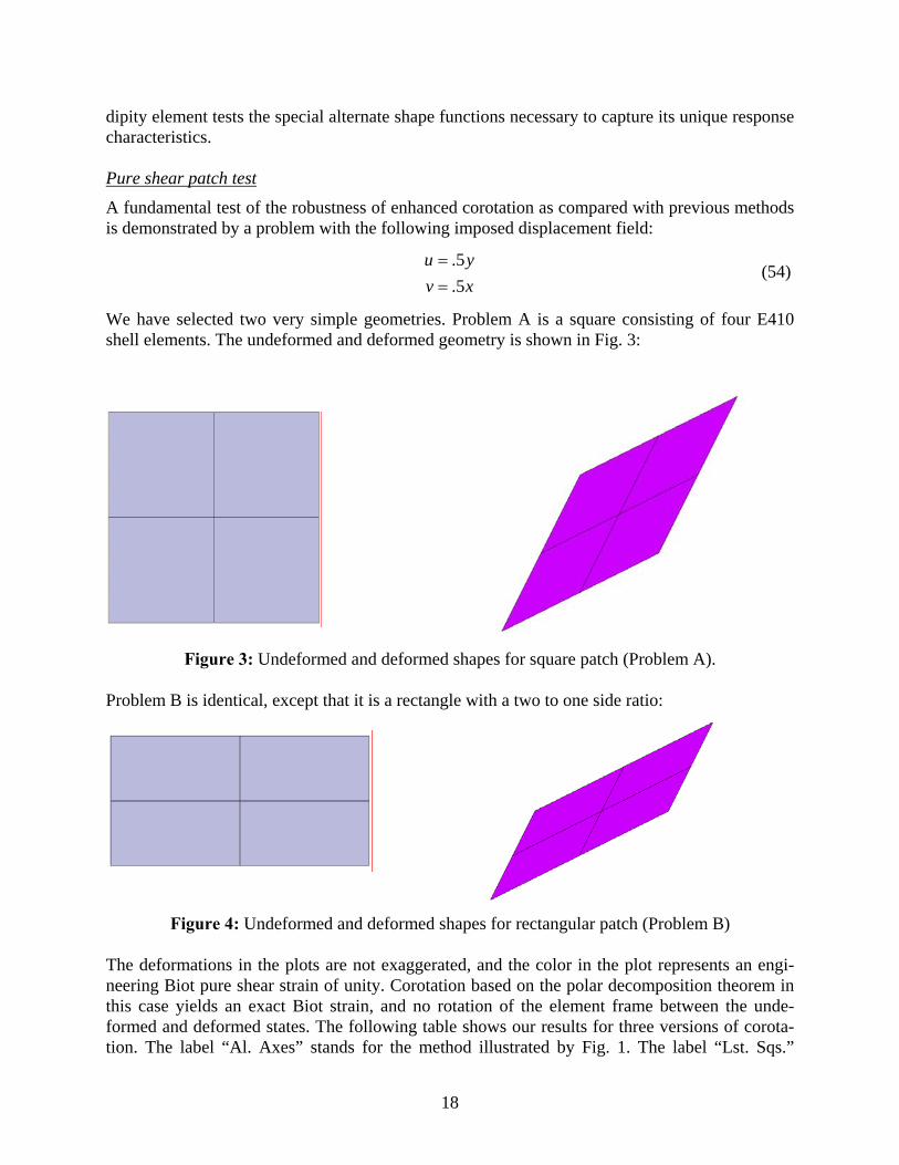
We have selected two very simple geometries. Problem A is a square consisting of four E410 shell elements. The undeformed and deformed geometry is shown in Fig. 3:

Figure 3: Undeformed and deformed shapes for square patch (Problem A).

Problem B is identical, except that it is a rectangle with a two to one side ratio:

Figure 4: Undeformed and deformed shapes for rectangular patch (Problem B) The deformations in the plots are not exaggerated, and the color in the plot represents an engi-neering Biot pure shear strain of unity. Corotation based on the polar decomposition theorem in this case yields an exact Biot strain, and no rotation of the element frame between the unde-formed and deformed states. The following table shows our results for three versions of corota-tion. The label “Al. Axes” stands for the method illustrated by Fig. 1. The label “Lst. Sqs.”

19

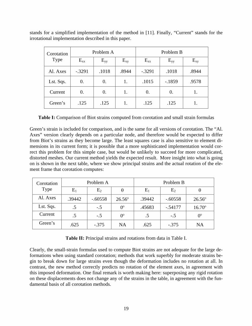
stands for a simplified implementation of the method in [11]. Finally, “Current” stands for the irrotational implementation described in this paper.

Problem A Problem B Corotation Type Exx Eyy Exy Exx Eyy Exy

Al. Axes -.3291 .1018 .8944 -.3291 .1018 .8944

Lst. Sqs. 0. 0. 1. .1015 -.1859 .9578

Current 0. 0. 1. 0. 0. 1.

Green’s .125 .125 1. .125 .125 1.

Table I: Comparison of Biot strains computed from corotation and small strain formulas

Green’s strain is included for comparison, and is the same for all versions of corotation. The “Al. Axes” version clearly depends on a particular node, and therefore would be expected to differ from Biot’s strains as they become large. The least squares case is also sensitive to element di-mensions in its current form; it is possible that a more sophisticated implementation would cor-rect this problem for this simple case, but would be unlikely to succeed for more complicated, distorted meshes. Our current method yields the expected result. More insight into what is going on is shown in the next table, where we show principal strains and the actual rotation of the ele-ment frame that corotation computes:

Problem A Problem B Corotation Type E1 E2 θ E1 E2 θ

Al. Axes .39442 -.60558 26.56° .39442 -.60558 26.56° Lst. Sqs. .5 -.5 0° .45683 -.54177 16.70° Current .5 -.5 0° .5 -.5 0° Green’s .625 -.375 NA .625 -.375 NA

Table II: Principal strains and rotations from data in Table I.

Clearly, the small-strain formulas used to compute Biot strains are not adequate for the large de-formations when using standard corotation; methods that work superbly for moderate strains be-gin to break down for large strains even though the deformation includes no rotation at all. In contrast, the new method correctly predicts no rotation of the element axes, in agreement with this imposed deformation. One final remark is worth making here: superposing any rigid rotation on these displacements does not change any of the strains in the table, in agreement with the fun-damental basis of all corotation methods.

20

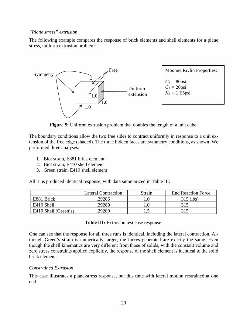
“Plane stress” extrusion

The following example compares the response of brick elements and shell elements for a plane stress, uniform extrusion problem:

Figure 5: Uniform extrusion problem that doubles the length of a unit cube. The boundary conditions allow the two free sides to contract uniformly in response to a unit ex-tension of the free edge (shaded). The three hidden faces are symmetry conditions, as shown. We performed three analyses:

1. Biot strain, E881 brick element. 2. Biot strain, E410 shell element 3. Green strain, E410 shell element

All runs produced identical response, with data summarized in Table III:

Lateral Contraction Strain End Reaction Force E881 Brick .29285 1.0 315 (lbs) E410 Shell .29289 1.0 315 E410 Shell (Green’s) .29289 1.5 315

Table III: Extrusion test case response.

One can see that the response for all three runs is identical, including the lateral contraction. Al-though Green’s strain is numerically larger, the forces generated are exactly the same. Even though the shell kinematics are very different from those of solids, with the constant volume and zero stress constraints applied explicitly, the response of the shell element is identical to the solid brick element. Constrained Extrusion

This case illustrates a plane-stress response, but this time with lateral motion restrained at one end:

Symmetry Free

Uniform extension

1.0

1.0 1.0

Mooney Rivlin Properties: C1 = 80psi C2 = 20psi Kb = 1.E5psi

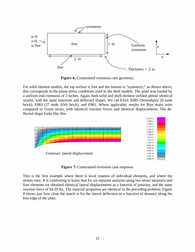
21

Figure 6: Constrained extrusion case geometry. For solid element models, the top surface is free and the bottom is “symmetry,” as shown above; this corresponds to the plane-stress conditions used in the shell models. The plate was loaded by a uniform end extension of 2 inches. Again, both solid and shell element yielded almost identical results, with the same reactions and deflected shapes. We ran E410, E885 (Serendipity 20 node brick), E883 (27 node ANS brick), and E881. Where applicable, results for Biot strain were compared to Green strain, with identical reaction forces and identical displacements. The de-flected shape looks like this:

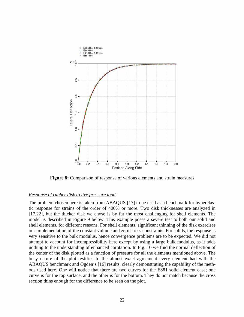
Figure 7: Constrained extrusion case response. This is the first example where there is local rotation of individual elements, and where the strains vary. It is comforting to know that for six separate analyses using two strain measures and four elements we obtained identical lateral displacements as a function of position, and the same reaction force of 64.29 lbs. The material properties are identical to the preceding problem. Figure 8 shows just how close the match is for the lateral deflection as a function of distance along the free edge of the plate:

u=0 v=0 w free

symmetry

free

free

2. in

1. in Uniform extension

Thickness = .2 in

u

v

Contours: lateral displacement.

22

Figure 8: Comparison of response of various elements and strain measures Response of rubber disk to live pressure load

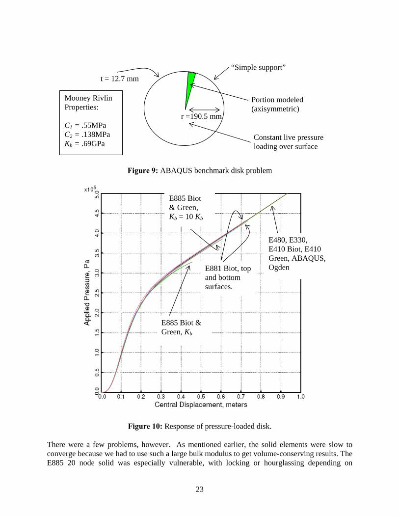
The problem chosen here is taken from ABAQUS [17] to be used as a benchmark for hyperelas-tic response for strains of the order of 400% or more. Two disk thicknesses are analyzed in [17,22], but the thicker disk we chose is by far the most challenging for shell elements. The model is described in Figure 9 below. This example poses a severe test to both our solid and shell elements, for different reasons. For shell elements, significant thinning of the disk exercises our implementation of the constant volume and zero stress constraints. For solids, the response is very sensitive to the bulk modulus, hence convergence problems are to be expected. We did not attempt to account for incompressibility here except by using a large bulk modulus, as it adds nothing to the understanding of enhanced corotation. In Fig. 10 we find the normal deflection of the center of the disk plotted as a function of pressure for all the elements mentioned above. The busy nature of the plot testifies to the almost exact agreement every element had with the ABAQUS benchmark and Ogden’s [16] results, clearly demonstrating the capability of the meth-ods used here. One will notice that there are two curves for the E881 solid element case; one curve is for the top surface, and the other is for the bottom. They do not match because the cross section thins enough for the difference to be seen on the plot.

23

Figure 9: ABAQUS benchmark disk problem

Figure 10: Response of pressure-loaded disk.

There were a few problems, however. As mentioned earlier, the solid elements were slow to converge because we had to use such a large bulk modulus to get volume-conserving results. The E885 20 node solid was especially vulnerable, with locking or hourglassing depending on

E881 Biot, top and bottom surfaces.

E885 Biot & Green, Kb = 10 Kb

E885 Biot & Green, Kb

E480, E330, E410 Biot, E410 Green, ABAQUS, Ogden

Constant live pressure loading over surface

t = 12.7 mm “Simple support”

Portion modeled (axisymmetric)

r =190.5 mm

Mooney Rivlin Properties: C1 = .55MPa C2 = .138MPa Kb = .69GPa

24

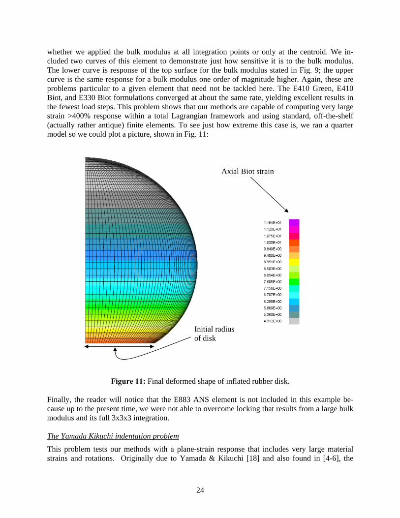
whether we applied the bulk modulus at all integration points or only at the centroid. We in-cluded two curves of this element to demonstrate just how sensitive it is to the bulk modulus. The lower curve is response of the top surface for the bulk modulus stated in Fig. 9; the upper curve is the same response for a bulk modulus one order of magnitude higher. Again, these are problems particular to a given element that need not be tackled here. The E410 Green, E410 Biot, and E330 Biot formulations converged at about the same rate, yielding excellent results in the fewest load steps. This problem shows that our methods are capable of computing very large strain >400% response within a total Lagrangian framework and using standard, off-the-shelf (actually rather antique) finite elements. To see just how extreme this case is, we ran a quarter model so we could plot a picture, shown in Fig. 11:

Figure 11: Final deformed shape of inflated rubber disk. Finally, the reader will notice that the E883 ANS element is not included in this example be-cause up to the present time, we were not able to overcome locking that results from a large bulk modulus and its full 3x3x3 integration. The Yamada Kikuchi indentation problem

This problem tests our methods with a plane-strain response that includes very large material strains and rotations. Originally due to Yamada & Kikuchi [18] and also found in [4-6], the

Axial Biot strain

Initial radius of disk

25

problem consists of a rectangular block with a uniform indentation on its left top half, allowed to slide but otherwise restrained on three edges, and free on its top right half:

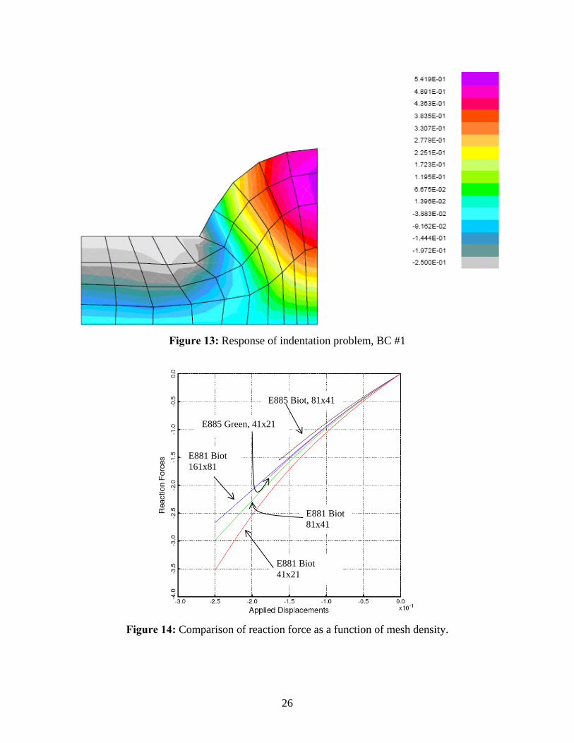
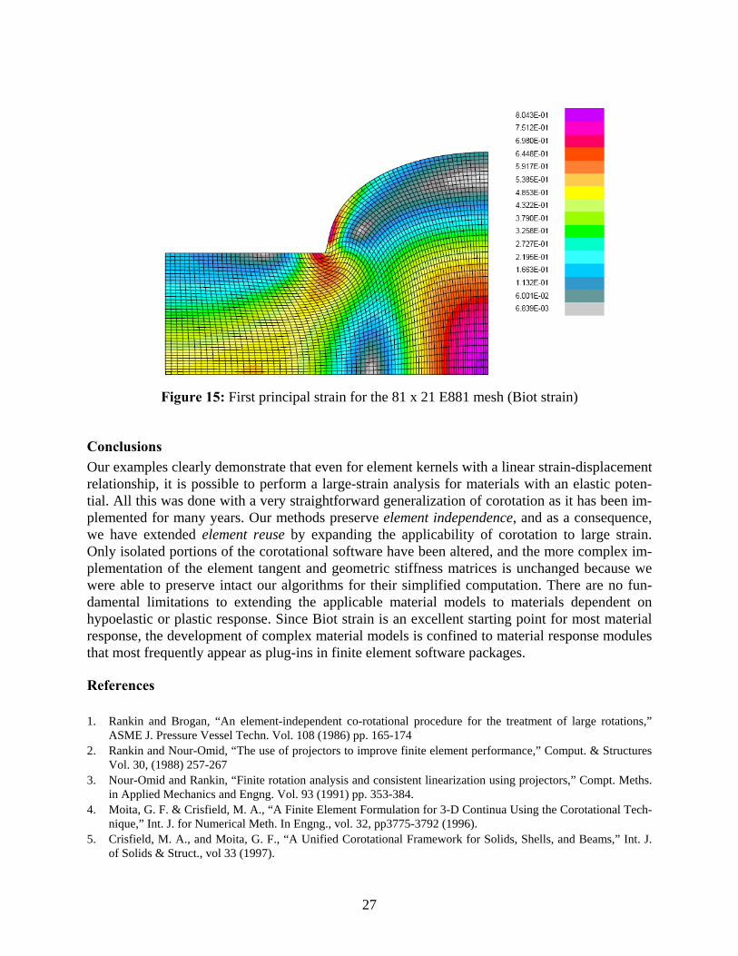
Figure 12: Indentation plane-strain problem geometry The imposed displacement boundary condition requires careful consideration. In our results, dis-placements parallel to the loaded edge (heavy black line) are permitted. This boundary condition is not the same as having a heavy steel plate push on the material and allowing the material to squeeze out. Rather, it means the nodes are free to move along the edge, which also allows the loaded section itself to expand or contract. The boundary condition is the same as the one used by Moita [4], which for a rather coarse grid like the one he used is displayed in Figure 13. The element in this picture is a plane-strain form of the E410, with our solid elements giving essen-tially the same results. Colors represent vertical displacements, and as in our previous examples, deformed shapes are not scaled. The reader will note the strong similarity with Figure 14 in [4]. To get a better understanding of this problem, we conducted a mesh refinement study using the total reaction force on the loaded segment as the measure of convergence. Figure 14 summarizes a series of analyses with two solid elements and two strain measures. Clearly convergence is slow, as would be expected if response in the area adjacent to the loaded edge (where strains vary significantly over a very short range) determines convergence. Figure 15 shows an example of a much finer grid and the huge distortions near the reentrant corner. We had serious problems with ill-conditioning and locking, especially for the E410 which became useless for the finer mesh models. Although we were able to extend the utility of the E881 brick by applying the bulk modulus term to the centroid only, doing the same thing for E885 caused hourglassing, just as in the ABAQUS disk. However, as in previous examples, these are element kernel details not ger-mane to either the effectiveness or the implementation of enhanced corotation.

Uniform applied displacement Free edge

2.

1. Thickness =.2 w= 0

Mooney Rivlin Properties: (non-dimensional) C1 = 1.5 C2 = 2.0 Kb = 1.E5

1.

26

Figure 13: Response of indentation problem, BC #1

Figure 14: Comparison of reaction force as a function of mesh density.

E885 Biot, 81x41

E885 Green, 41x21

E881 Biot 161x81

E881 Biot81x41

E881 Biot 41x21

27

Figure 15: First principal strain for the 81 x 21 E881 mesh (Biot strain)

Conclusions Our examples clearly demonstrate that even for element kernels with a linear strain-displacement relationship, it is possible to perform a large-strain analysis for materials with an elastic poten-tial. All this was done with a very straightforward generalization of corotation as it has been im-plemented for many years. Our methods preserve element independence, and as a consequence, we have extended element reuse by expanding the applicability of corotation to large strain. Only isolated portions of the corotational software have been altered, and the more complex im-plementation of the element tangent and geometric stiffness matrices is unchanged because we were able to preserve intact our algorithms for their simplified computation. There are no fun-damental limitations to extending the applicable material models to materials dependent on hypoelastic or plastic response. Since Biot strain is an excellent starting point for most material response, the development of complex material models is confined to material response modules that most frequently appear as plug-ins in finite element software packages.

References 1. Rankin and Brogan, “An element-independent co-rotational procedure for the treatment of large rotations,”

ASME J. Pressure Vessel Techn. Vol. 108 (1986) pp. 165-174 2. Rankin and Nour-Omid, “The use of projectors to improve finite element performance,” Comput. & Structures

Vol. 30, (1988) 257-267 3. Nour-Omid and Rankin, “Finite rotation analysis and consistent linearization using projectors,” Compt. Meths.

in Applied Mechanics and Engng. Vol. 93 (1991) pp. 353-384. 4. Moita, G. F. & Crisfield, M. A., “A Finite Element Formulation for 3-D Continua Using the Corotational Tech-

nique,” Int. J. for Numerical Meth. In Engng., vol. 32, pp3775-3792 (1996). 5. Crisfield, M. A., and Moita, G. F., “A Unified Corotational Framework for Solids, Shells, and Beams,” Int. J.

of Solids & Struct., vol 33 (1997).

28

6. Crisfield, M. A., Non-linear Finite Element Analysis of Solids and Structures – Vol. 2 Advanced Topics, Chap-ter 18. John Wiley & Sons, Inc., New York (1997).

7. Nygard and Bergan, “Chapter 10: Advances in treating large rotations for nonlinear problems,” in State-of the Art Surveys on Computational Mechanics, pp. 305-332.

8. Jetteur, P. H. & Cescotto, S., “A Mixed Finite Element for the Analsis of Large Inelastic Strains,” Int. J. for Num. Meth. In Engng., vol 31, pp229-239 (1991)

9. Simo, J. C. & Armero, F., “Geometric Nonlinear Enhanced Strain Mixed Method and the Method of Incom-patible Modes,” Int. J. for Num. Meth. In Engng., vol 33, pp1413-1449 (1992).

10. C. A. Felippa and B. Haugen, “A unified formulation of small-strain corotational finite elements: I. Theory,” CMAME vol 194, pp. 2285--2336 (2005)

11. DeVeubeke, “The Dynamics of Flexible Bodies,” Int. J. Engng. Sci., Vol. 14 (1976) pp. 895-913 12. C. Rankin, “On the Choice of Best Possible Corotational Element Frame,” in: S.N. Atluri, P.E. O’Dohoghue

(Eds.), Modeling and Simulation Based Engineering, Tech Science Press, Palmdale, CA (1998) 13. Biot, M., Mechanics of Incremental Deformations, pp. 6-8. John Wiley & Sons, Inc., New York (1965). 14. Crisfield, M. A., Non-linear Finite Element Analysis of Solids and Structures – Vol. 2 Advanced Topics, Chap-

ter 13. John Wiley & Sons, Inc., New York (1997). 15. Rankin, C. C., Brogan, F. A., Loden, W. A., Cabiness, H. D., “STAGS User Manual – Version 5.0,” Rhombus

Consultants Group, Inc., Palo Alto, CA, revised January 2005 (on-line). Previously Report No. LMSC P032594, Lockheed Martin Missiles and Space Company, Palo Alto, CA.

16. Ogden, J. T., Finite Elements of Nonlinear Continua, McGraw-Hill (1972) 17. ABAQUS 6.4 Benchmarks Manual, Section 1.1.7. 18. Yamada, T. & Kikuchi, F., “An Arbitrary Lagrangian-Eulerian Finite Element Method for Incompressible Hy-

perelasticity,” Comput. Methods in Appl. Mech. Engng., Vol 102, pp149-177 (1993). 19. Stanley, G. M., “Continuum-Based Shell Elements,” PhD Dissertation, Dept. of Mechanical Engineering, Stan-

ford University (1985). 20. Madenci, E. & Barut, A., “A free-formulation-based flat shell element for non-linear analysis of thin composite

structures,” Vol. 37, pp. 3825-3842 (1993). 21. K. C. Park, E. Pramono, G. M. Stanley, and H. A. Cabiness, “The ANS shell elements: Earlier developments

and recent improvements.” In Ahmed K. Noor, Ted Belytschko, and Juan C. Simo, editors, Analytical and Computational Models of Shells, pp. 217-239. American Society of Mechanical Engineers, New York, N.Y. (1989).

22. Hughes, T. J. R., and E. Carnoy, “Nonlinear Finite Element Shell Formulation Accounting for Large Membrane Strains,” Nonlinear Finite Element Analysis of Plates and Shells, AMD, vol. 48, pp. 193-208 (1981).