The Pennsylvania State University

The Graduate School

College of Engineering

COMBINED AIRFLOW AND ENERGY SIMULATION PROGRAM

FOR BUILDING MECHANICAL SYSTEM DESIGN

A Thesis in

Architectural Engineering

by

Atila Novoselac

© 2004 Jing Song

Submitted in Partial Fulfillment of the Requirements

for the Degree of

Doctor of Philosophy

May 2005

The thesis of Atila Novoselac was reviewed and approved* by the following:

Jelena Srebric Assistant Professor of Architectural Engineering Thesis Adviser Chair of Committee

Stanley A. Mumma Professor of Architectural Engineering

William P. Bahnfleth Associate Professor of Architectural Engineering John Mahaffy Associate Professor of Nuclear Engineering Richard A. Behr Professor of Architectural Engineering Head of the Department of Architectural Engineering

*Signatures are on file in the Graduate School.

iii

ABSTRACT

Energy and airflow programs are the main tools for designing energy efficient and

healthy buildings. Therefore, the goal of this thesis is to develop new models and improve

existing models for simulating energy and air flows in buildings.

Indoor airflow simulation programs calculate most of the parameters needed to evaluate

thermal comfort and indoor air quality. However, it is necessary that airflow simulation

programs have correct boundary conditions, which can be provided by energy simulation (ES)

programs. In order to develop simulation tools for precise evaluations of thermal comfort and

indoor air quality in buildings, the existing Computation Fluid Dynamics (CFD) airflow program

is improved by adding new models for the calculation of thermal boundary conditions.

Subsequently, this program is coupled with the newly-developed ES program.

This thesis considers different methods for coupling ES and CFD programs with

particular attention given to boundary conditions on enclosure surfaces, which connect the

modeling domains of these two programs. Three different coupling approaches were investigated

with special consideration given to accuracy and computation time. The results show that the

Integrated Coupling Method provides the optimum compromise between accuracy and

computation time.

In order to improve the accuracy of the calculations of thermal boundary conditions on

building internal surfaces, experiment-based convection correlations are implemented in the

CFD program. In the process, new convection correlations are developed based on

measurements conducted in a state-of-the-art experimental facility. Correlations for

characteristic surfaces in rooms with: cooled ceiling panels, displacement ventilation, or high

aspiration diffusers are developed.

Furthermore, additional experiments are performed to collect data so as to validate new

models for calculating thermal boundary conditions. A comparison of numerical and

experimental results shows that the new models for thermal boundary conditions calculation,

implemented in CFD, perform substantially better than wall functions. A certain level of grid

dependency of heat flux calculation with new models still exists. However it is much smaller

than with wall functions.

Finally, this thesis provides examples, which demonstrate that the coupled ES and CFD

program is an effective tool for the evaluation of energy consumption, thermal comfort, and air

quality in buildings.

iv

TABLE OF CONTENTS

LIST OF FIGURES.....................................................................................................................vii LIST OF TABLES....................................................................................................................... xi NOMENCLATURE ...................................................................................................................xii ABBREVIATIONS................................................................................................................... xiv ACKNOWLEDGEMENTS.........................................................................................................xv CHAPTER 1 INTRODUCTION .................................................................................................1

1.1 General Statement of Problem ........................................................................................1 1.2 Basic Properties of Energy Simulation and Indoor Airflow Programs ............................2 1.3 Research Objective and Thesis Outline ...........................................................................5

CHAPTER 2 CURRENT DESIGNEE TOOLS FOR BUILDING ENERGY AND AIRFLOW SIMULATIONS ..................................................................................7

2.1 Energy Simulation Programs ...........................................................................................7 2.1.1 Weighting Factor Method versus Energy Balance Method ..................................8 2.1.2 Integrated Method versus Loads-Systems-Plant Method .....................................9 2.1.3 HVAC System Models .......................................................................................11

2.2 Airflow Simulations Programs.......................................................................................12 2.2.1 Multi-zone Methods............................................................................................12 2.1.2 Computational Fluid Dynamic Methods.............................................................13

2.3 Integration of ES and CFD Models................................................................................16 2.3.1 Convective Heat Flux Problems .........................................................................18 2.3.2 Numerical Stability and Heat Flux Conservation in-between Two Domains .....20

CHAPTER 3 DEVELOPMENT OF NEW ENERGY SIMULATION PROGRAM.................22 3.1 Introduction....................................................................................................................22 3.2 Heat Transfer Models for Energy Subsystems...............................................................23

3.2.1 Boundary Conditions at External Surfaces .........................................................23 3.2.2 Boundary Conditions at Internal Surfaces ..........................................................30 3.2.3 Energy Equations for Building Systems .............................................................38 3.2.4 Inter-zone Airflow and Infiltration ....................................................................42 3.2.5 HVAC Models ...................................................................................................43

3.3 Numerical Models for ES Equations..............................................................................49 3.3.1 Discretization ......................................................................................................49 3.3.2 System of Equations ...........................................................................................54

3.4 Model for Simultaneous Load Calculation and HVAC Performance Simulation .........62 3.4.1 Coupled versus Not-Coupled Load and HVAC Calculation ..............................62 3.4.2 Coupling Approaches of Load and HVAC Models ............................................63 3.4.3 Constraints Control Algorithm............................................................................65

3.5 Validation.......................................................................................................................68 3.5.1 Validation of Program Components ...................................................................68 3.5.2 Verification of New ES program Using BESTEST............................................70

3.6 Summary ........................................................................................................................77

v

CHAPTER 4 AIR FLOW PROGRAM - BOUNDARY CONDITIONS...................................78 4.1 Introduction....................................................................................................................78 4.2 Fundamentals of CFD Programs....................................................................................79

4.2.1 RANS Equations, Turbulent Models, and Boundary Conditions .......................79 4.2.2 Numerical Discretization ....................................................................................87

4.3 Improvement of CFD Program for Indoor Air-flow Calculation...................................93 4.3.1 Modification of Adaptive Convection Algorithm...............................................93 4.3.2 Calculation of Referent Temperatures ................................................................94 4.3.3 Implementation of MACA into CFD..................................................................97 4.3.4 Convection Correlations Implemented into MACA ...........................................98 4.3.5 MACA Algorithm ............................................................................................ 103

4.4 Validation of MACA ................................................................................................... 106 4.5 Discussion and Summary............................................................................................. 113

CHAPTER 5 COUPLING OF ENERGY SIMULATION AND AIR FLOW PROGRAMS .. 114 5.1 Introduction.................................................................................................................. 114 5.2 ES and CFD Programs Coupling Methods .................................................................. 114

5.2.1 One-Directional Coupling Method ................................................................... 115 5.2.2 Two-Directional Coupling Methods ................................................................. 116

5.3 Comparison of Different Coupling Methods .............................................................. 120 5.3.1 Definition of a Numerical Test Case................................................................. 120 5.3.2 Performance of the Fully-Dynamic Coupling for the Numerical Test Case..... 121 5.3.3 Performance of the Quasi-Dynamic Coupling for the Numerical Test Case.... 123 5.3.4 Performance of the Integrated Coupling for the Numerical Test Case ............. 124 5.3.5 Performance of the One-Directional Coupling for the Numerical Test Case ... 125

5.4 Summary ...................................................................................................................... 126

CHAPTER 6 ORGANIZATION AND GRAPHICAL USER INTERFACE OF COUPLED PROGRAM ..................................................................................... 127

6.1 Introduction.................................................................................................................. 127 6.2 Data Flow in Coupled ES and CFD Program .............................................................. 127 6.3 GUI Preprocessor ......................................................................................................... 130 6.4 GUI Postprocessor ....................................................................................................... 136 6.5 Summary ...................................................................................................................... 139

CHAPTER 7 DEVELOPMENT OF NEW CONVECTION CORRELATIONS .................... 140

7.1 Introduction.................................................................................................................. 140 7.2 Convection Correlations Development ........................................................................ 141 7.3 Convection Correlation at Cooled Ceiling Panels........................................................ 145 7.4 Convection Correlations in a Room with High Aspiration Diffuser............................ 147 7.5 Convection Correlations in a Room with Displacement Ventilation ........................... 153 7.6 Discussion and Summary............................................................................................. 158

CHAPTER 8 LABORATORY MEASUREMENTS AND ANALYSIS ................................ 160

8.1 Introduction.................................................................................................................. 160 8.2 Experimental Facility ................................................................................................... 160

8.2.1 Environmental and Climate Chambers ............................................................. 161 8.2.2 Measuring Equipment ....................................................................................... 163

8.3 Measurements for Convection Correlations Development .......................................... 166 8.3.1 Measurements of Convection Coefficients at Cooled Ceiling Surfaces ........... 169

vi

8.3.2 Measurements of Convection Coefficients in Rooms with High Aspiration Diffusers................................................................................. 170 8.3.3 Measurements of Convection Coefficients in Rooms with Displacement Ventilation.................................................................................. 172

8.4 Measurements for MACA Validation .......................................................................... 173 8.5 Measurements for Evaluation of CFD Models for IAQ and Thermal Comfort Study 174 8.6 Uncertainties of the Measurements .............................................................................. 176 8.7 Summary ...................................................................................................................... 181

CHAPTER 9 APPLICATION OF THE COUPLED PROGRAM........................................... 182

9.1 Introduction.................................................................................................................. 182 9.1.1 The Effect of Thermal Boundary Conditions on Concentration Distribution... 182 9.1.2 Chapter outline.................................................................................................. 183

9.2 Comparison of Contaminant Removal Effectiveness and Air Exchange Efficiency . 184 9.2.1 Properties of Air Exchange Efficiency and Contaminant Removal Effectiveness ..................................................................................................... 184 9.2.2 Analyzed Cases ............................................................................................... 187 9.2.3 Results and analysis ......................................................................................... 191 9.2.4 Summary of Analysis of εa and ε ...................................................................... 193

9.3 Energy and Thermal Comfort Analysis of DV System Combined with CC Panels . 194 9.3.1 Model Room ..................................................................................................... 194 9.3.2 Results and Discussion ..................................................................................... 195

9.4 Discussion and Summary ............................................................................................. 201 CHAPTER 10 CONCLUSIONS AND RECOMMENDATIONS FOR FUTURE WORK .... 202

10.1 Conclusions................................................................................................................ 202 10.2 Recommendations for Future Work ......................................................................... 205 REFERENCES .......................................................................................................................... 206 APPENDIX A: Angles of Solar Radiation............................................................................... 213 APPENDIX B: View Factor Calculation ................................................................................. 215 APPENDIX C: Coefficients of Zone-matrix Equations ........................................................... 217 APPENDIX D: Sparse Matrix Solver....................................................................................... 220 APPENDIX E: View Factors and Diffuse and Direct Solar Radiation Distribution................ 224 APPENDIX F: Material Specification for Test Building ......................................................... 226 APPENDIX G: CFD Coefficients ............................................................................................ 228 APPENDIX H: Example of Results for Experimental Validation of CFD Models ................. 229

vii

LIST OF FIGURES

Figure 1.1 Modeling domains for Energy Simulation (ES) and Airflow (CFD) programs......... 3 Figure 2.1 Influence of type and position of the HVAC device in a room on the selection of surface convection correlation (Beausoleil 2000) ...........................19 Figure 3.1 Building heat flow mechanisms implemented in a new building energy simulation (BES) program .......................................................................................23 Figure 3.2 Solar radiation on the external surface of a building................................................25 Figure 3.3 Geometry of a building facade used in the shading model for solar radiation calculation................................................................................................................27 Figure 3.4 External surface convection and long wave radiation on the external surfaces of buildings ................................................................................................................29 Figure 3.5 Distribution of direct solar radiation on internal room surfaces...............................35 Figure 3.6 Distribution of diffuse solar radiation and shortwave radiation from lights on internal room surfaces.........................................................................................36 Figure 3.7 Transmission, absorption, and reflection on internal surfaces ................................39 Figure 3.8 Heat transfer for a double glazed window implemented into the BES program......40 Figure 3.9 Different models for lamp heat flow for (a) lamps with cover, (b) lamps without cover, and (c) free hanging lamps ..............................................................41 Figure 3.10 Schematic for a model of a simple air handling unit................................................44 Figure 3.11 Schematic for a radiant panel heat transfer model ...................................................47 Figure 3.12 Discretization of a building zone in the BES program.............................................49 Figure 3.13 Discretization of a non-homogeneous zone elements in the BES program .............50 Figure 3.14 Energy balance of an element-inner node ................................................................50 Figure 3.15 Energy balance for an element’s surface node.........................................................52 Figure 3.16 Two-dimensional model of a room discretization....................................................56 Figure 3.17 The example zone matrix for a two-dimensional model presented in Figure 3.16 ..57 Figure 3.18 Two-dimensional model of a room with a controlled source of energy (QHVAC) .....57 Figure 3.19 Zone matrixes for a room (zone) with a controlled source of energy (QHVAC) .........58 Figure 3.20 Two-dimensional model of a room with controlled supply air (Qsupply_air)...............58 Figure 3.21 Zone matrix for a room (zone) with controlled supply air .......................................59 Figure 3.22 An example model of a room with two zones: (1) room and (2) plenum zones ......60 Figure 3.23 A zone matrix for room and plenum zones ..............................................................60 Figure 3.24 Air and radiant panel temperature in a room when (a) separate and (b) integrated load and HVAC models are used..............................................................................62 Figure 3.25 Structure of a zone and HVAC matrix where HVAC models are integrated into the zone matrix ........................................................................................................64 Figure 3.26 Schematic of a simultaneous solution scheme implemented into the BES program .....................................................................................................64 Figure 3.27 Constraints control algorithm implemented into the BES program .........................66 Figure 3.28 A comparison of analytical end numerical solutions for the temperature distribution with unsteady heat transfer in a homogeneous wall ................................................69 Figure 3.29 Room geometry for energy conservation tests .........................................................69 Figure 3.30 Energy conservation tests for unsteady heat transfer ...............................................70 Figure 3.31 BESTEST comparison results for annual diffuse and direct incident solar radiation at different surface orientations ...............................................................72 Figure 3.32 BESTEST comparison results for annual transmitted diffuse and direct solar radiation through a south oriented window with and without window shading overhang..........................................................................72

viii

Figure 3.33 BESTEST comparison results for diagnostic test cases - heating............................73 Figure 3.34 BESTEST comparison results for diagnostic test cases - cooling............................73 Figure 3.35 BESTEST comparison results for qualification test cases - heating ........................74 Figure 3.36 BESTEST comparison results for qualification test cases -cooling.........................74 Figure 4.1 Velocity distributions on a surface...........................................................................85 Figure 4.2 Finite-volume discretization of a room ....................................................................88 Figure 4.3 Finite volume discretizations for upwind scheme....................................................88 Figure 4.4 Reference temperatures used in MACA for convective heat flux calculations in a CFD program ........................................................................................................94 Figure 4.5 Velocity and temperature distributions in the boundary layer on vertical room surfaces ....................................................................................................................95 Figure 4.6 Local temperature calculations for vertical surfaces ................................................95 Figure 4.7 Boundary layers for horizontal room surfaces. ........................................................96 Figure 4.8 Temperature profile for (a) totally and (b) locally strafed room air.........................98 Figure 4.9 Surface heat flux distribution with Dirichlet and Neumann boundary conditions ...98 Figure 4.10 MACA algorithm ................................................................................................... 104 Figure 4.11 Temperature stratification in a room with cooled ceiling and displacement ventilation.........................................................................................106 Figure 4.12 Stand positions (1 to 6) for temperature measurements .........................................108 Figure 4.13 A comparison of measured and calculated temperature profiles for Case1: Sun patch at floor, all air system - 3.8 ACH...........................................................109 Figure 4.14 A comparison of measured and calculated temperature profiles for Case2: Convective heat source, air system combined by cooled ceiling - 1.7 ACH.........110 Figure 4.15 A comparison of measured and calculated temperature profiles for Case3: Heated wall, all air system - 1.8 ACH ...................................................................111 Figure 4.16 Grid dependency for MACA and wall functions for three different grid resolutions in the vicinity of a surface ...................................................................112 Figure 5.1 One-directional coupling of ES and CFD programs ..............................................116 Figure 5.2 Heat flux on surfaces in the ES and CFD domains ................................................116 Figure 5.3 Quasy Dynamic Coupling of ES and CFD programs.............................................118 Figure 5.4 Fully Dynamic Coupling of ES and CFD programs ..............................................119 Figure 5.5 Integrated Coupling of ES and CFD programs ......................................................119 Figure 5.6 Geometry of the test room for comparison of different coupling methods (source 1 – computer simulator, source 2 – humans simulator) .............................120 Figure 5.7 Temperature and cooling load for the test case used for coupling methods comparison.............................................................................................................121 Figure 5.8 Cooling loads for the test case calculated using the fully-dynamic coupling method ....................................................................................................122 Figure 5.9 Cooling load calculations for different time steps with the quasi-dynamic coupling .................................................................................................................123 Figure 5.10 Comparison of computation time for the fully-dynamic and integrated coupling .124 Figure 6.1 Data flow diagram for the coupled program ..........................................................128 Figure 6.2 Data flow diagrams for cases where the coupled program is used for only a) energy or b) airflow simulation .........................................................................129 Figure 6.3 GUI of the coupled program representing model geometry, and two basic window forms...............................................................................................131 Figure 6.4 The toolbar of coupled programs for the selection of the simulation (a) type, (b) parameters..........................................................................................132

ix

Figure 6.5 Different types of surface discretization definitions (a) surface definition in GUI, (b) surface definition in typical CFD and ES programs, (c) internal GUI surface definition.........................................................................132 Figure 6.6 Surface positioning and type selection (temperature wall, heat flux surface, adiabatic surface, window, supply, exhaust, radiant panel, and lighting)..............133 Figure 6.7 Windows form for specification of surface object properties ................................134 Figure 6.8 Windows form for mesh generation presenting room geometry and regions defined by internal room objects ...........................................................................135 Figure 6.9 Windows form for HVAC system selection (variations of: all-air, all-water, or combined water air system)...............................................................................135 Figure 6.10 Location selection and surface properties of ground or surrounding objects.........136 Figure 6.11 A segment of output files of the BES program ......................................................137 Figure 6.12 New 3D visualization tools developed for presentation of results obtained from the CFD0 or coupled program ......................................................................138 Figure 6.13 Windows form of new 3D visualization tools for the set up of graphical parameters...............................................................................................139 Figure 7.1 An experimental facility for the development of convection correlations .............141 Figure 7.2 Energy balance on internal surfaces of an experimental facility............................142 Figure 7.3 Combined convection coefficients for natural and forced convections ................144 Figure 7.4 Temperature profiles near a cooled ceiling and a heated floor ..............................145 Figure 7.5 Measured air temperature profiles for pure convective and surface heat sources............................................................................................................146 Figure 7.6 Experimental results used for the development of cooled ceiling convection correlations..........................................................................................147 Figure 7.7 High aspiration diffuser providing a narrow jet with high entrainment of room air .............................................................................................................149 Figure 7.8 Forced convection correlation for walls in a room with high aspiration diffuser ..................................................................................................150 Figure 7.9 Forced convection correlation for floor in a room with high aspiration diffuser ..................................................................................................150 Figure 7.10 Forced convection correlation for a ceiling in a room with high aspiration diffuser .................................................................................................151 Figure 7.11 Natural convection for vertical surfaces in a room with no ventilation .................152 Figure 7.12 Natural convection for floor surfaces where Tfloor>Tair and there is no ventilation in a room.........................................................................................152 Figure 7.13 Air flow and temperature stratification in a room with displacement ventilation..153 Figure 7.14 Measured convection coefficients for the floor in rooms with DV as a function of local temperature difference (∆T) and supply volume flow rate (ACH)...........154 Figure 7.15 Forced convection correlations for the floor in rooms with a DV diffuser including the convection coefficients measured at heat patch surfaces ...............156 Figure 7.16 Comparison of new developed correlation (Equation 7.14) with other correlations used for convective heat flux calculation on cooled ceiling surfaces 158 Figure 8.1 A schematic of climate and environmental chambers............................................161 Figure 8.2 A schematic of water-flow and air-flow in climate and environmental chambers.162 Figure 8.3 Control system of building energy and an environmental systems facility............163 Figure 8.4 Interface of an air-velocity measuring system .......................................................164 Figure 8.5 Interface of a data acquisition system used for temperature measurements...........164 Figure 8.6 Interface of a tracer gas measuring system based on gas chromatography ............165 Figure 8.7 Experimental set-ups for (a) Climate and (b) Environmental chambers ................166

x

Figure 8.8 The (a) positioning and (b) constriction of a pure convective heat source used for convection correlation development ........................................................167 Figure 8.9 Positions of stands with temperature sensors in an environmental chamber .........168 Figure 8.10 A temperature recording to determine steady-state conditions ..............................169 Figure 8.11 Distribution of surface heating/cooling devices in experiments for MACA validations ..........................................................................................173 Figure 8.12 Uncertainty for measured convection coefficient at cooling panels ......................179 Figure 8.13 Uncertainty for measured convection coefficient on floors in a room with displacement ventilation diffuser...................................................................180 Figure 9.1 A comparison of the measured concentrations with CFD results when (1) wall functions are used for heat flux calculation and (2) measured heat fluxes are used as boundaries ..................................................................................................183 Figure 9.2 Normalized local age of air and contaminant concentration distributions for similar airflow field and different positions of the contaminant source............185 Figure 9.3 Space layouts with supply and exhaust positions for the analyzed cases................187 Figure 9.4 Spatial distributions of the age of air (τ) and different contaminants (C) in a segment of a large cubicle office .....................................................................190 Figure 9.5 Positions of the occupied zone and breathing plane................................................191 Figure 9.6 The correlation between air exchange efficiency and contaminant removal effectiveness ...........................................................................................................192 Figure 9.7 Position of the model room in the building (Figure a) with geometry and positions internal heat sources (Figure b) ...............................................................194 Figure 9.8 Characteristic temperatures and extracted energy for the model room with a DV/CC system for a period of 7 days as calculated by the BES program...........196 Figure 9.9 Cooling load and temperatures in model rooms with a DV/CC system for a period of 7 days as calculated by the BES program ......................................197 Figure 9.10 The effect of the minimum CC surface temperature on air temperature and cooling load in a model room ................................................................................198 Figure 9.11 Air temperature and cooling load in the model room with a DV/CC system as calculated by the BES program and by the coupled program ...........................198 Figure 9.12 Daily change of temperature gradient in the model room with a CC/DV system..199 Figure 9.13 Spatial distribution of the thermal comfort index PPD in the model room with a DV/CC system ............................................................................................200 Figure 9.14 Daily change of the thermal comfort index PPD in the model room with a DV/CC system ............................................................................................200 Figure 9.15 Use of the coupled program for periodic thermal comfort and air quality analysis ..................................................................................................................201 Figure A.1 Solar angles for vertical and horizontal surfaces....................................................213 Figure B.1 View factor for parallel surfaces ...........................................................................215 Figure B.2 View factor for orthogonal surfaces .......................................................................216 Figure D.1 A zone matrix of energy equations ........................................................................220 Figure D.2 Sub-matrices for four zone elements......................................................................221 Figure D.3 The second matrix ..................................................................................................221 Figure D.4 Modified sub-matrices............................................................................................222 Figure D.5 Modified second matrix..........................................................................................222 Figure D.6 Modified second matrix after Gaussian elimination ..............................................223 Figure E.1 Test building geometry ..........................................................................................224 Figure H.1 Geometry of the room and positions of air temperature sensors ............................229 Figure H.2 Positions of characteristic surfaces with surface temperature sensors ...................229

xi

LIST OF TABLES Table 3.1 Convection correlations for mixed, forced, and natural convection (Beausoleil 2000)........................................................................................................31 Table 3.2 Fractions for diffuse radiation distributions ...............................................................37 Table 3.3 Annual peak cooling and heating loads ......................................................................75 Table 4.1 Variables constants and sources for the general transport equation (4.20).................84 Table 4.2 Alamdari and Hammond convection correlations ......................................................99 Table 4.3 Khalifa convection correlations................................................................................100 Table 4.4 Fisher convection correlations 100 Table 4.5 Fisher and Pedersen convection correlations............................................................101 Table 4.6 Awbi and Hatton convection correlations ................................................................101 Table 4.7 Correlations for ventilation with displacement ventilation diffuser .......................102 Table 4.8 Correlations for ventilation with high aspiration diffuser ........................................103 Table 4.9 Types of airflow regime ...........................................................................................104 Table 4.10 Surface types ............................................................................................................105 Table 4.11 Comparison of convective heat flux calculated by MACA and wall functions .......107 Table 5.1 Properties of heat sources and the HVAC system for the test room..........................120 Table 8.1 Measurement results for cooled ceiling surfaces......................................................170 Table 8.2 Measurement results for the room with a high aspiration diffuser and cooled ceiling .....................................................................................................171 Table 8.3 Measurement results for the floor surface in a room with displacement ventilation ...........................................................................................172 Table 8.4 Characteristic data of cases used for experimental validation of MACA.................174 Table 8.5 The cases for experimental validation of CFD models ............................................175 Table 9.1 Air exchange efficiency for characteristic ventilation flow types ............................185 Table 9.2 Limits for air exchange efficiency and contaminants removal effectiveness ...........186 Table 9.3 Simulation parameters for the studied cases of four room types..............................189 Table 9.4 Properties of heat sources of the model room ..........................................................195 Table E.1 View factors for the test building (room) ................................................................224 Table E.2 Direct solar radiation distribution for the test building (room) and ε = 0.6 ..........225 Table E.3 Diffuse solar radiation distribution from Window 1 (ε = 0.6 ) ................................225 Table E.4 Diffuse solar radiation distribution from Window 2 (ε = 0.6 ) ...............................225 Table F.1 Material specifications for lightweight BESTEST cases (Judkoff and Neymark 1995)...................................................................................226 Table F.2 Material specifications for heavyweight BESTEST cases (Judkoff and Neymark 1995)...................................................................................227 Table G.1 Coefficients for hybrid differencing schemes..........................................................228 Table G.2 Convection and diffusion coefficients .....................................................................228 Table H1 Surface temperatures and heat fluxes ......................................................................230 Table H2 Air temperatures measured in an occupied zone [°C] .............................................231 Table H3 Air temperatures and velocities measured in the vicinity of surfaces .....................231 Table H4 Tracer gas concentration in occupied zone -represented as (C-Cin)/(Cout-Cin) .........231

xii

NOMENCLATURE

A - surface area ACH - number of room air changes per hour Ai - anisotropy index

AL - effective air leakage cp - specific heat Dh - hydraulic diameter of cooling surfaces E - cooling coil effectiveness F’- radiant panel efficiency factor Fi,j - view factors from surface 'i' to surface 'j' g - gravitational constant g - gravity acceleration Gr - Grashof number h - surface convection coefficient IDIR - direct solar radiation IDNR - direct normal radiation IGHR - global horizontal radiation J - radiosity k - conductivity k - turbulent kinetic energy L - characteristic length m - mass flow rate Nu - Nusselt number P - power p - pressure Pr - Prandl number Q - heat flux q - specific heat flux R - conductive resistance r - re-circulated air portion Re - Reynolds number Sc - Schmidt number T - temperature u - local velocity in the vicinity of the surface U - wind speed V - velocity w - humidity ratio ν - kinematic viscosity σt - turbulent Prandtl number α − absorptivity µ - viscosity Γ - effective diffusivity δ - boundary layer thickness θ - incident angle ρ - density - reflectance ψi,j - radiative heat exchange factors from surface 'i' to surface 'j'

xiii

∆T - temperature difference ∆xp - distance from wall to the adjacent cell centre ∆τ - time step β - thermal expansion coefficient or the surface slope ε - contaminate removal effectives - surface emissivity - dissipation rate of turbulent energy εa - air exchange efficiency φ - general variable µt - turbulent viscosity τ - time

xiv

ABBREVIATIONS

ACA - Adaptive Convection Algorithm ACH - Air Changes per Hour AHU - Air Handling Unit ASHRAE - American Society of Heating Refrigerating and Air-Conditioning Engineers BES - Newly Developed Building Energy Simulation Software CAV - Constant Air Volume CFD - Computational Fluid Dynamics CFD0 - Research CFD software CPU - Central Processing Unit DDC - Direct Digital Control DNS - Direct Numerical Simulation DOAS - Dedicated Outdoor Air System DV - Displacement Ventilation ES - Energy Simulation ESP-r - Commercial Energy Simulation Software FLUENT - Commercial CFD software GUI - Graphical User Interface HVAC - Heating Ventilating and Air-Conditioning IAQ - Indoor Air Quality IGU - Model for Insulated Glazing Units LES - Large Eddy Simulation MACA - Modified Adaptive Convection Algorithm MIT - Massachusetts Institute of Technology PHOENICS - Commercial CFD software RANS - Raynold's Average Navier-Stokes equations RNG - k-ε model based on Renormalization Group SIMPLE - Semi-Implicit Method for the Pressure-Linked Equations TMY2 - Typical Metrological Year Weather Database VAV - Variable Air Volume

xv

ACKNOWLEDGEMENTS

First, I would like to offer my gratitude to my thesis advisor, Professor Jelena Srebric for

her support and guidance. She actively encouraged, motivated, and challenged me throughout

the completion of this thesis. With her highly positive attitude she helped me to become more

independent researcher.

Next, I would like to thank Ivana Veljkovic, Akhil Kamat, and Brendon Burley. They

are students from the Pennsylvania State University, and they have been of a great help to me

with this thesis. Ivana Veljkovic, a PhD student at the Computer Science and Engineering

Department, developed the graphical user interface for software developed as a part of this

thesis; Akhil Kamat, a student at Computer Science and Engineering Department, developed a

3D visualization tool for software result presentation; and Brendon Burley, a student at the

Architectural Engineering Department, helped me with the experimental measurements that were

conducted as a part of this thesis.

Last but not least, I would like to acknowledge the counseling and assistance given by

my thesis committee members: Professor Stanley Mumma, Professor William Bahnfleth, and

Professor John Mahaffy.

1

CHAPTER 1

INTRODUCTION

1.1 General Statement of Problem

People spend most of their time in buildings. Hence, issues related to the indoor

environment, such as indoor air quality (IAQ) and thermal comfort, are of great public concern.

Poor IAQ and inadequate thermal comfort in buildings adversely affect the health condition of

occupants (NIOSH 2004). Furthermore, recent incidents related to bioterrorism (anthrax attacks)

and the fast spread of infectious diseases (SARS), have triggered many concerns about the control

of the indoor environment. Building heating, ventilating, and air-conditioning (HVAC) systems

provide control of major parameters related to the indoor environment. To evaluate and improve

IAQ and thermal comfort resulting from HVAC systems, airflow simulation programs are used.

These are programs based on Computational Fluid Dynamics (CFD) or zonal modeling.

Improvements made to building HVAC systems can provide direct and indirect economic

benefits. Direct benefits relate to the reduction of energy consumption, and indirect benefits are

related to increased productivity and reduction of medical expenses. In addition, lower energy

consumption in buildings can significantly reduce the emission of CO2 because buildings use

around 50% of the total energy consumption in developed countries (Harris and Eliot, 1997, DOE

2004) Therefore, any analysis of building HVAC system that can effectively reduce this

consumption is highly valuable. In order to evaluate and reduce energy consumption in the design

phase of building, energy simulation (ES) programs are used.

It is commonly believed that improvements made to indoor air quality must lead to an

increase in energy consumption. This is the case when the air quality is improved by a simple

increase of fresh air supply. With careful selection of an HVAC system, building materials, and

air-distribution devices, IAQ can be improved and energy consumption can be reduced

simultaneously. To achieve this worthy goal, air flow simulation and ES programs are used for

energy consumption, thermal comfort and IAQ analyses. At present, most of these analyses are

performed with separate ES and air flow programs. However, because of the interaction between

building elements and air temperature distribution, a building’s air and energy flows should be

considered together by using combined ES and airflow programs.

2

Separate applications of ES and airflow programs usually provide acceptable results for

certain types of analysis. However, many assumptions used in these programs decrease the

accuracy of programs when they are used separately. For example, accuracy of an airflow

program results is highly sensitive to the boundary conditions assumed (or eventually measured)

by the user (Emmerich 1997, Xu and Chen 1998). The reason for this is that the flow inside the

airflow simulation domain (i.e. a room) is driven by the boundary conditions. Also, the

assumption in an ES program of uniform air temperature in the room can cause imprecise

calculation of convective heat fluxes on room surfaces. This can lead to large inaccuracy in

energy consumption calculations since different convection coefficients models can create

difference in cooling load calculation up to 27% for the same test case (Lomas 1995). An

integration of ES and airflow programs can eliminate many of these assumptions, since the

information provided by ES and airflow programs are complementary related to boundary

conditions (refer to Section 1.2). With coupling ES and air flow programs, increased accuracy in

both programs is achieved.

The development of ES and air flow programs is connected to the development of

computer technologies. The fast development of computing power has enabled the use of more

complex models for air-flow and energy-flow simulations. In addition, the current speed of

computing enables the combination of ES and air flow programs for specific analyses on a

personal computer. Extensive research has been conducted in order to reach the point that air-

flow and energy-flow systems are combined in the analysis of a single building. The next section

describes only basic properties of these programs, while Chapter 2 provides a detailed literature

review on the development of ES, air flow, and combined programs.

1.2 Basic Properties of Energy Simulation and Indoor Airflow Programs

Building Energy Simulation (ES) programs are tools used for the analysis of building

energy consumption and the evaluation of architectural designs. These tools are used for

modeling heating, cooling, and ventilating flows in a building. The modeling domain of the ES

program (Figure 1.1) comprises of:

- Building envelope,

- Heating Ventilating and Air-Conditioning (HVAC) systems,

- External and internal parameters, such as weather conditions or occupancy level

- Indoor air represented as uniform thermal mass for a particular zone.

3

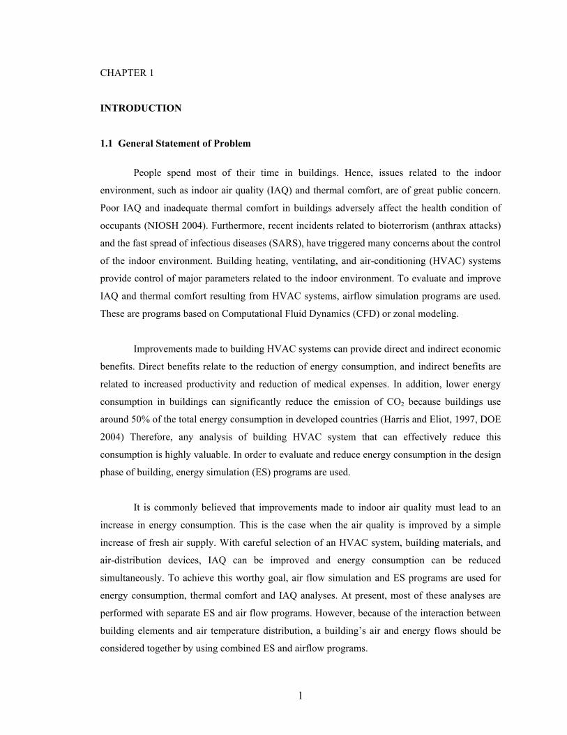
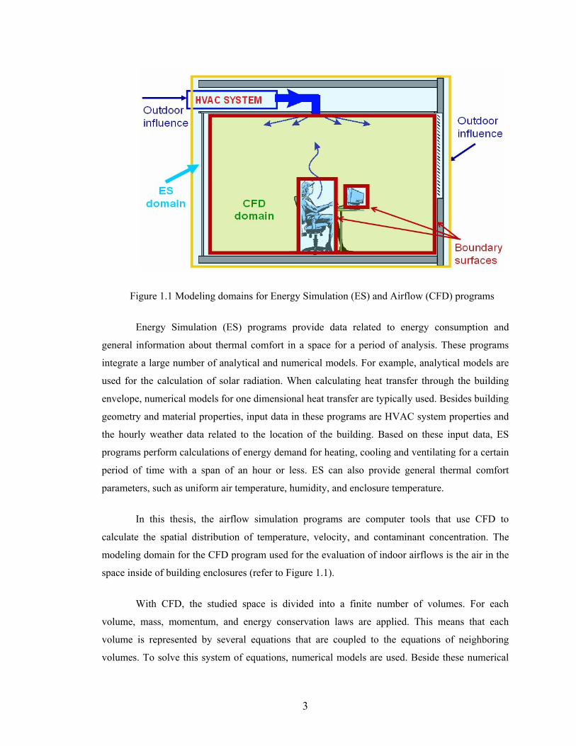
Figure 1.1 Modeling domains for Energy Simulation (ES) and Airflow (CFD) programs

Energy Simulation (ES) programs provide data related to energy consumption and

general information about thermal comfort in a space for a period of analysis. These programs

integrate a large number of analytical and numerical models. For example, analytical models are

used for the calculation of solar radiation. When calculating heat transfer through the building

envelope, numerical models for one dimensional heat transfer are typically used. Besides building

geometry and material properties, input data in these programs are HVAC system properties and

the hourly weather data related to the location of the building. Based on these input data, ES

programs perform calculations of energy demand for heating, cooling and ventilating for a certain

period of time with a span of an hour or less. ES can also provide general thermal comfort

parameters, such as uniform air temperature, humidity, and enclosure temperature.

In this thesis, the airflow simulation programs are computer tools that use CFD to

calculate the spatial distribution of temperature, velocity, and contaminant concentration. The

modeling domain for the CFD program used for the evaluation of indoor airflows is the air in the

space inside of building enclosures (refer to Figure 1.1).

With CFD, the studied space is divided into a finite number of volumes. For each

volume, mass, momentum, and energy conservation laws are applied. This means that each

volume is represented by several equations that are coupled to the equations of neighboring

volumes. To solve this system of equations, numerical models are used. Beside these numerical

4

models, building airflow simulation programs use models that are based on experimental data.

These experiment-based models are integrated into the CFD program code and used for the

prediction of human responses to various air velocities and temperatures. Beside space geometry,

input data in these airflow simulation programs are surface contaminant emission, surface thermal

properties and properties of supplied air, such as volume flow rate, temperature and

concentration. With these input data, the CFD numerical solver calculates temperature, velocity,

and contaminant concentration for each finite volume of the analyzed space. These data enable

detailed analyses of thermal comfort and air quality.

Coupling of ES and CFD programs occurs at boundary surfaces, which are the domains

between these two programs. The ES calculates the temperature of the surfaces, which constitute

input data for the CFD program. On the other side, the CFD program calculates convective heat

fluxes based on velocity and temperature fields near the surfaces. These convective heat fluxes

are defined by near- surface (local) air temperatures and by convective coefficients. To satisfy the

energy balance, heat fluxes at all surfaces have to be the same when they are calculated for the ES

and CFD program domains. Therefore, the CFD provides to the ES local air temperatures and

convective coefficients which constitute input data for this program. Besides enclosure

temperatures, the ES provides to the CFD program input data related to boundary conditions at

thermal objects, such as occupants and computers, if any. Boundary conditions for thermal

devices are defined by air velocity, temperature, and concentration for air supply thermal devices,

or by surface temperature or heat flux for devices like radiant panels, baseboard heaters, and

computers. By the consecutive exchange of information at the boundary domains between these

two programs, increasingly accurate input data are provided for each program.

For the calculation of convective heat flux, the CFD can use wall functions or convection

experimental-based expressions. Log-law wall functions, which are based on the correlation

between velocity and temperature field in the boundary layer, are extensively used in CFD

applications to calculate convective heat flux. However, wall functions are inaccurate for flow

driven by natural convection which is a predominant type of flow on building surfaces. Therefore,

this thesis is also focused on alternative methods for the calculation of heat flux. These methods

include the application of convection correlations, which are based on experimental results.

5

1.3 Research Objective and Thesis Outline

The objective of this thesis is to enhance indoor air and energy flow modeling in the

context of simulation of all building systems. Improvement of indoor air and energy flow

modeling includes the following:

(1) ES and CFD programs coupling, with special attention given to the

-development of a method which satisfies the energy balance between two program domains and

-use of accurate surface heat transfer models;

(2) Further development of models for surface heat transfer calculations on buildings’ internal

surfaces;

(3) Development of new methods for simultaneous load calculations and HVAC performance

simulation that enables a modular approach for HVAC system modeling;

(4) Analysis of different indoor air quality parameters for their use in coupled ES and CFD

programs.

In order to gather knowledge of existing models for ES and air flow simulations, a critical

review of existing literature was conducted. The review of these models is presented in Chapter 2,

with a special focus on integrated modeling approaches that were used as a basis for further

developments in this thesis.

As a part of this thesis, a new ES program was developed and used as a platform for

coupling with air flow programs. This ES program incorporates existing and newly developed

building system simulation models. It also implements a new method for simultaneous load

calculations and HVAC performance simulations. Details about the newly developed ES program

are presented in Chapter 3 with a special focus on methods for simultaneous load calculations and

HVAC performance simulations.

An existing CFD program (Srebric 2000) was used for coupling with the new ES

program. This CFD program was further developed in order to implement models for accurate

6

boundary conditions calculations. Details about CFD models are provided in Chapter 4 with a

focus on new models for thermal boundary conditions.

Chapter 5 contains details about three different methods for the coupling of ES and CFD

programs. It contains comparative analyses of these methods, with a discussion about the

respective advantages and disadvantages of each method.

To enable easy use of the coupled ES and CFD program a new graphical user interface

(GUI) for this program was developed in collaboration with students mentioned in

acknowledgments. Basic details about the new GUI and structure of the coupled program are

provided in Chapter 6.

New convection correlations were developed as part of this thesis in order to improve the

performance of experiment-based models for the calculation of thermal boundary conditions in

CFD program. Chapter 7 contains the experimental results and details about these newly

developed convection correlations.

In order to develop new convection correlations, full-scale laboratory experimental

measurements were performed. Also, measurements for the validation of new models for thermal

boundary conditions calculation in the CFD program and measurements for coupled code

validations were conducted. Details about these measurements are presented in Chapter 8.

Chapter 9 presents application examples for the coupled program. It contains an analysis

of thermal comfort and energy consumption of displacement ventilation systems, combined with

cooling radiant panels. Also, this chapter contains an analysis of different IAQ parameters.

Finally, Chapter 10 summarizes the work presented in this thesis, and provides

recommendations for further research.

7

CHAPTER 2

CURRENT DESIGN TOOLS FOR BUILDING ENERGY AND AIRFLOW

SIMULATIONS

In this chapter, a critical overview of energy simulation and airflow programs is given.

This overview focuses on their respective advantages and disadvantages when these programs are

applied in analyses of buildings. In addition, other researchers’ efforts of coupling these two types

of programs are considered. Finally, the two most recently proposed models for the coupling of

energy simulation and airflow programs are critically analyzed in detail to explore the respective

advantages and disadvantages of both models.

2.1 Energy Simulation Programs

Until the mid 1960s, only simple manual methods were used to estimate energy usage in

buildings. Two of the most widely used manual methods are the degree day method and the bin

method. The simplest method is the degree day method, which is based on the averaging of

outdoor weather influence over a long period of time (ASHRAE Fundamentals 2001). This

method was successfully used for rough estimations of heating energy requirements. For more

detailed heating and cooling analysis, the bin method was used. This method calculates energy

over several intervals (bins) of temperature using a simplified quasi-steady-state approach

(ASHRAE Fundamentals 1985). Besides very limited accuracy, these simple manual methods

could not provide any information about thermal comfort such as enclosure temperature and air

temperature when the heating/cooling system does not work.

More detailed energy simulation methods include sophisticated models of a building and

its HVAC systems. These methods are computationally intensive and require extensive use of

computers. Today, there is a larger variety of Energy Simulation (ES) programs with building

system models of various complexities.

For building heating/cooling load calculation, ES programs may use the:

- Weighting factor method, or

- Energy balance method.

8

To integrate of HVAC models with heating/cooling load calculation models, ES

programs may use the:

- integrated method, or

- Loads-System-Plant method.

Considering the complexity of HVAC models, ES programs may use the following three

methods for HVAC system simulation and energy consumption calculations:

- psychometric chart zoning method,

- whole-building simulation method, or

- component-based simulations method.

2.1.1 Weighting Factor Method versus Energy Balance Method

In the calculation of the heating/cooling load, the thermal mass of the building has to be

considered. Because of the thermal capacity, the heat gains and cooling loads in the analyzed

building zone are different. Therefore, unsteady heat conduction needs to be solved for each

element of the building enclosure. The weighting factor and the heat balance methods are the two

approaches used for these calculations.

The weighting factor method estimates the ratio of convective heat transfer to the total

incoming energy on a building element during a time period. Weighting factors depend on

building material properties and they are usually pre-calculated for certain types of building

elements. Based on the structure of a building element, the ES program selects an appropriate

weighting factor and calculates the convective load. Programs based on the weighting factor

method do not need extensive computations. They were, therefore, popular during the 1970’s

when the computer power was very limited. The ES programs that use weighting factors are:

NESCAP (NASA 1975), DOE-1 (Diamond et al. 1977), DOE-2 (Birdsall et al. 1985), and

VISUAL DOE-3 (Visual DOE 3.1 2003).

The energy balance method is based on the heat balance for zone air and enclosure

elements. With this method, conductive, convective, and radiative heat fluxes are in balance for

each surface. Equations for surface heat balance are usually linearized (radiation terms) and

organized into a surface balance matrix. After the matrix is solved, the cooling load for the

considered zone is determined. BLAST (Hittle 1979), ACCURACY (Chen et al. 1988), ESP-r

(Clarke et al. 1985) and EnergyPlus (Crawley 2000) are ES programs based on the energy

9

balance method. Relative to the coupling of ES and airflow programs, the energy balance method

has an advantage when compared to the weighting factor method. This is due to the fact that the

room surface convective coefficient can vary across the enclosure and room air temperature can

be non-uniform. Furthermore, energy balance method has advantages over weighting factor when

thermal comfort and moisture transport is considered. Enclosure surface temperatures computed

by the energy balance method can be used for thermal comfort evaluation and radiant heating and

cooling systems analyses. Also, temperature distributions in building elements calculated by the

energy balance method enable the study of moisture transport (Crawley et al. 2001).

Depending on how the conduction through building elements is solved, energy balance

programs may use:

- discretization methods or

- conduction transfer functions.

Commonly used discretization methods are finite volume and finite difference methods,

where the enclosure elements are discretized (one-dimensionally) into a finite number of nodes.

Energy balance equations for building discretization nodes create a system of equations organized

in a matrix which is numerically solved. The solution of this system provides the cooling/heating

load, surface temperature, and temperatures inside each element of the building enclosure. ESP-r

(Clarke 1985) uses this discretization method.

Programs that use conduction transfer functions calculate heat fluxes and surface

temperatures based on the “history” of surface temperatures. The energy balance matrix for this

method is simpler than the matrix with discretization methods because only surface nodes are

considered. However, the stability limits of conduction transfer functions restrict this method to

analyses where small time steps are used (EnergyPlus 2001). Programs that use conduction

transfer functions are BLAST (Hittle 1979), ACCURACY (Chen et al. 1988), and EnergyPlus

(Crawley 2000).

2.1.2 Integrated Method versus Loads-Systems-Plant Method

Earlier generations of energy simulation (ES) programs have not integrated models of

HVAC systems into the cooling load calculation procedure. These programs use the Loads-

10

Systems-Plant (LSP) modeling strategy, which subdivides the simulation of the building into

three sequential steps:

1) the building’s heating and cooling loads are calculated for the analyzed period and

assumed set of indoor environmental conditions. These loads are then imposed as inputs

to the second step of the simulation.

2) the plant’s air handling and energy distribution systems are modeled. This simulation

step predicts the demands of the plant’s energy conversion systems such as boilers,

chillers and other related equipment.

3) the program calculates the energy required in the energy plant and estimates the cost of

this energy.

The most popular programs which use this method are DOE-2 (Birdsall et al. 1985) and BLAST

(Hittle 1979).

With the LSP approach, mass and energy balance equations which describe HVAC

systems are solved without iterations. In this way, the LSP method reduces computing costs by

using the values of key variables from the calculations in the previous time step. However, this

method does not provide the feedback information from HVAC systems to the heating/cooling

load calculation. The lack of the feedback has a potentially serious impact on the accuracy of

temperature and comfort predictions. As an example, in reality, when a central plant cannot

satisfy the demand for heating due to its limited capacity, temperatures in the zones will drop

below the set point. However, the LSP method assumes that central plants always have a large

enough capacity to maintain the temperature set point in the zone. Beside giving inaccurate

thermal comfort predictions, this assumption may affect the calculation of the heating/cooling

load because, in reality, temperature offsets from previous time steps affect the demand for

heating/cooling load in next time step.

The disadvantages of the LSP method stimulated the development of a new generation of

programs. These new programs employ simultaneous procedures for building load calculations

and HVAC performance simulations. This integrated method is implemented into the ESP-r

program (Clarke 1985) and EnergyPlus program (Crawley 2000). The integrated method requires

more computational time and more complex equation solvers than the LSP method. However, the

integrated solution technique with accurate predictions of space temperatures enables a more

reliable analysis of HVAC system performance and occupant comfort. This integrated analysis

11

enables predictions of realistic system controls, moisture transfer in building elements, and

performance of radiant heating and cooling systems.

2.1.3 HVAC System Models

HVAC system models use conservation of mass and energy to calculate the respective

cooling, heating, and electric energy demands of various components of the system. These

components include coils, pumps, fans, humidifiers, ducts, mixing boxes, chillers, boilers and

other HVAC components. Depending on each application, ES programs use methods of various

complexities for the required energy calculation.

Among available methods, psychometric chart zoning is the simplest. This method does

not explicitly simulate any component of the HVAC system. Weather data in the psychometric

chart are divided into several zones (Paassen 1986). Within each similar zone, the air handling

process is assumed to be the same. The annual energy consumed by an HVAC component in each

zone is equal to the energy required by the component multiplied by the time of operation.

Considering the integration of building and HVAC models, this method uses a simplified version

of the LSP method, known as the Loads-Plant method. Psychometric chart zoning is not very

accurate. However, it is very straightforward and easy to understand. ACCURACY (Chen et al.

1988) uses this method.

When simulating whole buildings, HVAC systems are preconfigured and program users

are offered fixed menus of common HVAC system configuration settings. For example, a user

can select the Variable Air Volume (VAV), Single Zone Variable Temperature or any other

typical HVAC system with the appropriate central plant configuration settings. In more powerful

versions of such simulations, the ES program user has the freedom to configure elements in air

handling units or power plants. Typical whole-building ES programs are DOE-2 (Birdsall et al.

1985), VISUAL DOE 3 (Visual DOE 3.1 2003), BLAST (Hittle 1979), and Energy Plus (Crawley

2000). However, with this method, the number of HVAC system configurations is still limited.

The most powerful models for energy calculations have component-based models. With

these programs, the user interconnects the models of HVAC components, freely creating his/her

own HVAC configuration. These programs focus on the performance of the HVAC system.

Therefore, they usually have less detailed building load models. Generally, component-based

12

programs have more accurate algorithms and, therefore, they are useful for detailed studies of

special systems. These systems include control systems and active solar heating/cooling systems.

Typical component-based programs are TRNSYS (Klein et al. 1994) and CLIMA 2000 (Gautier

et al. 1991). These most powerful procedures for HVAC systems analysis demand considerable

effort from the user for system modeling. They are also computationally expensive for buildings

with many zones undergoing long periods of analysis such as one year or more.

The simplicity of the whole-building simulation method and the HVAC precision of the

component-based method are complementary. Therefore, programs such as ESP-r (Clarke 1985)

combine strong points of these two types of programs. However, considering thermal comfort and

air quality, there is no significant difference between whole-building and component-based

methods because improvements in HVAC system simulations have very low impact on these

environmental parameters.

2.2 Airflow Simulations Programs

For indoor airflow simulations, the Multi-zone method and Computational Fluid

Dynamic (CFD) method are used. Each method has certain advantages and disadvantages related

to computation speed, accuracy, thermal comfort, and air quality prediction ability.

2.2.1 Multi-zone and Zonal Methods

Energy simulation (ES) programs and building airflow programs were developed at

approximately the same time. The initial models for indoor airflow simulations are based on

multi-zone methods. Jackman (1970) was one of the first researchers to use multi-zone network

airflow models for the simulation of building infiltration and the airflow between spaces. This

multi-zone method uses macroscopic models, which represent large air volumes such as rooms by

single nodes, and calculate the flow through discrete paths such as doors and cracks. On the other

hand, Lebrun (1970) used the related zonal method for room airflow simulations. The zonal

method splits a room into different zones and characterizes the main driving flows in order to

predict the spatial temperature distribution in the room. For both methods, multi-zone and zonal

methods, the principles of calculation are the same. The considered space (building or room) is

divided into sub-spaces (rooms or part of the rooms) in which only the conservations of mass and

13

energy are applied. The solution to this system of equations provides general information about

the considered airflow.

When the multi-zone method is applied to the simulation of airflows in-between rooms,

the program results include: infiltration rate, airflow between zones, and contaminant distribution.

Programs which use this approach are CONTAM (Dols 2003) and COMIS (Feustel 1998). These

programs require small computation time and are user-friendly in their operation. However, they

provide only general information about air quality since each zone (room) is assumed to have

uniform contaminant distribution. These programs do not provide any information about thermal

comfort. Furthermore, this method requires the temperature distribution in the building as input

data, which is difficult to know in advanced even for experienced program users. Many

simulations simply use measured on-site data if available or assume set-point temperature for

each building zone.

The zonal method used for room airflow simulations has been used in different studies

related to building airflow (Inard et al. 1996 and Musy et al. 2001). With this method, the

temperature distribution in the room is calculated. Therefore, this method provides more

information about thermal comfort than the multi-zone models that simulate only airflow between

zones (rooms). Similar to multi-zone models, zonal models also require small computing power.

However, this performance is highly dependent on assumptions related to boundary conditions

and experimental data. Therefore, the existing zonal models are limited only to general

predictions of mean temperatures and mass flow rates in each zones of the room.

2.2.2 Computational Fluid Dynamic Methods

Computational Fluid Dynamic (CFD) methods have been successfully applied in the

prediction of room airflow since the 1970’s. Nielsen (1989), and Jones et al. (1992) provide a

detailed reviews of CFD applications in building simulations. Due to high computational

requirements, a CFD analysis is usually restricted to single rooms or several spaces within

buildings. Typical outputs of a CFD simulation are three-dimensional spatial distributions of:

− air velocity for all three directional components,

− air temperature,

− relative humidity,

14

− turbulent intensity, and

− different contaminants concentration.

These CFD outputs enable considerably better air quality and thermal comfort analysis than any

multi-zone or zonal model.

The largest challenge of CFD modeling is the prediction of turbulent flows. Turbulence

can be characterized as a chaotic state of fluid motion. It is characterized in terms of irregularity,

diffusivity, large Reynolds numbers, three-dimensional vorticity fluctuations, dissipation and

continuum (Tennekes and Lumley 1972). Due to these features, it is difficult to establish whether

airflow in a room is an artificially induced, transitional, or fully developed turbulent. It is also

observed that very few room airflows are laminar.

Because all non-laminar room airflows can be defined as turbulent ones, the CFD

program used for airflow prediction requires appropriate models for turbulence. Generally,

turbulent flows are predicted by three approaches:

- Direct Numerical Simulation (DNS),

- Large Eddy Simulation (LES), and

- Turbulence transport models.

The DNS method requires very fine space discretization with cell size on the order of 10-3

m. In consideration of typical room sizes and computation power of today’s computers,

simulations of indoor airflows are not realistic with this method. The LES method was developed

by Deardorff (1970) who hypothesized that the turbulent motion could be separated into large and

small eddies and that the separation between these two does not have a significant effect on the

evolution of large eddies. Because this method assumes that small eddies are independent of the

flow geometry, the need for a very fine grid is eliminated. The main contribution to turbulent

transport comes from the large-eddy motion and, therefore, this method provides better results

than methods which are based on empirical turbulent transport models. Some successful

applications of LES related to building simulation are: the flow around a building (Murakami et

al. 1996, Jiang et al. 2003), jet flow (Voke et al. 1993), forced convection flow in a room

(Davidson et al. 1996, Emmerich et al. 1998), natural ventilation flow in buildings (Jiang at al

2001), and particle dispersion in buildings (Jiang et al. 2002). However, this method requires

large computer power and memory. Therefore, LES is still rarely applied for the simulation of

15

indoor airflows. Therefore, like DNS, LES requires computers that are more powerful than those

typically available today to be effectively applicable to room airflow simulation.

Because of the difficulties involved in deterministic turbulence models, turbulence

transport models are widely used in engineering applications. All the turbulence transport models

solve the Reynolds statistically averaged Navier-Stokes (RANS) equations. These models can be

generally divided into two categories:

- Reynolds stress models, and

- eddy-viscosity models.

Reynolds stress models use transport equations for the individual Reynolds stress, while

the eddy-viscosity models use Boussinesq approximation that relates Reynolds stress to the rate

of mean stream through an “eddy” viscosity (Wilcox 2000). Reynolds stress models are applied

to predict room airflow patterns in a room with jets (Renz et al. 1990). The results indicate that

the Reynolds stress model is superior to the standard k-ε model, which is eddy viscosity model,

because anisotropic effects of turbulence are taken into account. However, Chen (1996) compared

three Reynolds-stress models with the standard k-ε model for natural convection, forced

convection, mixed convection, and impinging jet in a room. He concluded that the Reynolds-

stress models are only slightly better than the k-ε model. Nevertheless, the Reynolds stress

models require three to ten times more computing time than the eddy-viscosity models because of

the greater algebraic complexity. With this increase of computing time and relatively small

improvement in indoor airflow prediction, Reynolds stress models are still very rarely applied in

building simulations.

Classic eddy-viscosity models include mixing-length models such as the zero equation,

one equation, and two equations eddy-viscosity model (Rodi 1993). The two equation model,

often referred to as the “standard” k-ε model, is the most widely-used turbulence model in

engineering practice. Here, k represents the turbulence kinetic energy, while ε represents the

dissipation rate of turbulence energy. There are several variations of k-ε model. Chen (1995)

tested five different k-ε models for natural convection, forced convection, mixed convection, and

impinging jet in a room. Chen found that it is very difficult to identify any other model superior

to the standard k-ε model. Many studies confirmed applicability of the k-ε model for thermal

comfort and indoor air quality analyses Nielsen (1998). However, there are many factors that

16

influence the results such as mesh generation, convergence procedure, and boundary condition

implementation. Therefore, a more powerful computer and a skilful user are necessary for an

effective and accurate simulation.

To decrease computational time, Chen and Xu (1998) developed a zero-equation model

specifically developed for modeling room airflows and heat transfer. This model uses an

algebraic equation to calculate the local eddy viscosity instead of differential equations for kinetic

energy (k) and dissipation rate (ε). This substantially reduces the computation time compared to

the more complex k-ε approaches. Chen and Xu (1998) tested this model on four airflow types:

displacement ventilation, natural ventilation, forced convection, and mixed convection. They

found good agreements between the zero-equation model predictions and the experimental data.

In fact, in some cases the zero-equation model outperformed the k-ε model. Srebric et al. (1999)

provided further validation of this approach by comparing the zero-equation model’s predictions

to experimental data for three additional cases of airflows in rooms. These included natural

convection with infiltration, forced convection, and mixed convection with displacement

ventilation. They found good agreement between the computed and measured air velocity and

temperature profiles.

2.3 Integration of ES and CFD Models

When CFD models are used alone for the prediction of indoor airflows, the user, besides

the enclosure geometry, provides the following boundary conditions:

- Convective heat flux or surface temperature at enclosure surfaces,

- Flow entering or leaving the room at enclosure openings.

These boundary conditions are based on known design data, measured data, and other

assumptions. Usually, known design data are volume flow rate at enclosure openings, such as air

volume flow at inlets and heat fluxes at certain surfaces such as computers or heaters. Other

assumptions are surface temperatures and volume flow at openings created by infiltration or

natural ventilation. The accuracy of airflow prediction is very sensitive to these assumed

boundary conditions (Awbi 1998 and Xu et al. 1998) because the flow inside the CFD domain

(room) is driven by the boundary conditions.

In the case where the building simulation program considers the whole building including

the HVAC systems and indoor air distribution, the boundary conditions are placed at the exterior

17

surfaces of the building. Boundary conditions are then derived from exterior conditions such as

temperature, solar radiation, wind velocity, humidity, and other relevant weather data. In this

way, the overall influence of dynamic weather conditions on airflows and HVAC system is

established. Considering this, CFD researchers have begun to integrate building models and inter-

surface radiation models into CFD codes (Holmes et al. 1990, Chen et al. 1995, and Moser et al.

1995). This type of CFD programs solves convective, radiative, and conductive heat transfer

simultaneously. This method is powerful, but it is also computationally very expensive (Chen et

al. 1995) because CFD treats heat transfer though building elements as a three-dimensional

unsteady conduction problem. Also, when CFD calculates the heat transfer in solid materials, the

calculation becomes stiffer and the computing time goes up dramatically (Thompson 1988).

Chen (1988) is probably the first researcher who tried to couple an ES program with a

CFD program. He showed that the coupling of ES and CFD programs can provide more accurate

predictions of cooling loads, especially in the case of stratified flows. Nielsen et al. (1998)

confirmed that an interconnection between these two programs would improve the energy

consumption calculation including an improvement in the prediction of thermal comfort and air

quality in a selected area of a building. Srebric et al. (2000) continued Chen’s study (1988) by

using coupling for dynamic heating/cooling load calculations. However, this coupling is a quasi-

dynamic coupling, which with large time-steps (time discretization) do not enforce heat flux

conservation in-between the CFD and ES calculation domains.

For the energy balance between the ES and CFD domains, a slightly better approach than

that of Srebric (2000) was used by Clarke et al. (1995) and Negrao et al. (1995), whereby a CFD

code was integrated into the ESP-r building simulation program. The two modeling domains

exchange information on a time step basis. The overall energy balance is then achieved through

an iterative procedure. This fully dynamic coupling increases accuracy, but the iterative

procedure considerably increases the computation time.

Recent progress in the coupling of ES and CFD programs was provided by Beausoleil et

al. (2000, 2001, 2003) and Zhai et al. (2001). Beausoleil continued Clarke’s (1995) and Negrao’s

(1995) work by focusing on improving the convective heat flux calculation between the ES and

CFD domains. Zhai at al (2001) continued Chen’s (1988) and Srebric’s (2000) work by

implementing the CFD into EnergyPlus. In these studies, they focused on numerical stability of

18

coupling models and heat flux conservation in-between the two domains. Since these two

research studies considered very important issues related to

- methods for accurate surface convective heat flux calculation and

- methods for coupling ES and CFD programs

which are complementary, the next two subsections present more details about these research

studies.

2.3.1 Convective Heat Flux Problems

In the integrated modeling approach, the ES and CFD domains interact on surfaces

(walls). However, in near-wall regions the CFD has difficulty performing accurate convective

flux calculations. With the k-ε models, standard log-law wall-functions (Launder and Spalding

1974) are usually used for wall shear and surface convection calculations. These wall-functions

only provide good results for a particular type of room airflow. Chen et al. (1990), Niu et al

(1992), and Awbi (1998) showed that the logarithmic profile poorly approximates velocities, and

especially surface convection, in the boundary layer for buoyancy-driven flows. This model is

sensitive to the location of the near-wall grid points. In principle, the smaller the first grid size,

the larger the calculated heat flux. Overall, log-law wall functions are valid only for forced

convention in near-wall regions.

To solve the boundary condition problem, Beausoleil (2000, 2001) created the “Adaptive

Convection Algorithm” and “Adaptive Conflation Controller”. These procedures combine

convection correlations and wall-functions models for the calculation of surface heat fluxes.

The adaptive convection algorithm calculates convection coefficients based on:

- Geometry, such as height of a wall and characteristic dimension of a room,

- Temperature of surface, supply air, and room air,

- Type and position of an HVAC device in a room (refer to Figure 2.1),

- Supplied air volume flow rates.

Based on these data, the adaptive convection algorithm dynamically assigns (for each

surface) an appropriate convection model from 24 experiment-based convection correlations.

Also, during the simulation, this algorithm monitors the operational state of the HVAC device

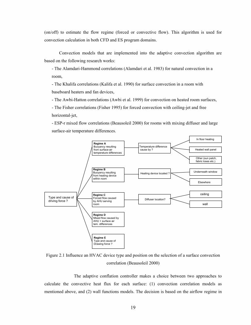
19

(on/off) to estimate the flow regime (forced or convective flow). This algorithm is used for

convection calculation in both CFD and ES program domains.

Convection models that are implemented into the adaptive convection algorithm are

based on the following research works:

- The Alamdari-Hammond correlations (Alamdari et al. 1983) for natural convection in a

room,

- The Khalifa correlations (Kalifa et al. 1990) for surface convection in a room with

baseboard heaters and fan devices,

- The Awbi-Hatton correlations (Awbi et al. 1999) for convection on heated room surfaces,

- The Fisher correlations (Fisher 1995) for forced convection with ceiling-jet and free

horizontal-jet,

- ESP-r mixed flow correlations (Beausoleil 2000) for rooms with mixing diffuser and large

surface-air temperature differences.

Figure 2.1 Influence an HVAC device type and position on the selection of a surface convection

correlation (Beausoleil 2000)

The adaptive conflation controller makes a choice between two approaches to

calculate the convective heat flux for each surface: (1) convection correlation models as

mentioned above, and (2) wall functions models. The decision is based on the airflow regime in

Type and cause of driving force ?

Regime A Buoyancy resulting from surface-air temperature differences

Regime E Type and cause of Drawing force ?

Temperature difference cause by ?

In floor heating

Heated wall panel

Other (sun patch, fabric loses etc.)

Underneath window

Elsewhere

ceiling

wall

Regime B Buoyancy resulting from heating devicewithin room

Regime C Forced flow causedby AHU serving room

Regime D Mixed flow caused by AHU + surface air tem. differences

Heating device located ?

Diffuser location?

20

the vicinity of considered surface. The ES and CFD programs operate independently, but

exchange information on the internal surfaces at the beginning of each simulation time step.

However, special boundary condition treatments were developed to improve surface conflation.

For each time step, the adaptive conflation controller first performs an investigative CFD

simulation to approximate the room’s airflow and temperature field. Subsequently, the controller

calculates dimensionless numbers (Re, Gr) that define the type of airflow on each surface. In this

process, the controller selects a model for the boundary condition calculations on each surface.

For example, the controller uses log-law wall functions for surfaces with only forced convection,

Yuan’s wall-functions (Yuan et al. 1993) for vertical surfaces with only natural convection, or

adaptive convection algorithm to select the appropriate convection correlation for all other flow-

types. Finally, with the new boundary conditions, the CFD calculates the final flow, temperature,

and concentrations distributions.

In the boundary condition calculation, this method provides highly accurate results.

However, the conflation controller requires a double run of the CFD calculation for each surface

temperature distribution provided by the ES program. This double run of CFD is computationally

expensive and requires a coupling method which does not provide the full coupling of the ES and

CFD programs. As a result, this type of coupling is time step sensitive and the Beausoleil (2000)

suggest a time step of 15 minutes or less.

Beausoleil’s research (Beausoleil 2000 and 2001) considerably improved the coupling.

However, he still did not completely resolve all the important issues. The adaptive conflation

controller improves the boundary condition calculations, but it limits the coupling of the ES and

CFD programs to one-directional coupling or quasy dynamic coupling. These two coupling

methods have certain weaknesses related to accuracy and sensitivity to calculation time step,

which are described in Chapter 5. Also, the adaptive convection algorithm needs additional

models to calculate convection coefficients. Most of the 24 convection correlations are applicable

to mixed air in a room. Surface convection models for stratified room airflows such as those with

displacement ventilation or flows in a room with chilled ceiling panels are not included.

2.3.2 Numerical Stability and Heat Flux Conservation in-between Two Domains

Zhai et al. (2001) and Chen et al. (2002) focused their research on integrated coupling.

They used the heat flux balance between two program domains for coupling in the ES and CFD

programs. For several modifications of fully dynamic coupling, these two researchers analyzed

21

convergence and stability problems that may occur in the coupled program due to different

mathematical and numerical models used in ES and CFD programs.

Considering information which describes the surface heat flux between two programs,

four different “data-type methods” were analyzed:

(1) ES to CFD by T; CFD to ES by h and ∆T

(2) ES to CFD by T; CFD to ES by hcorrected

(3) ES to CFD by T; CFD to ES by q

(4) ES to CFD by q; CFD to ES by h and ∆T

where ‘T’ is the interior surface temperature; ‘q’ is convective heat flux on interior surfaces; ‘h’ is

the convective heat transfer coefficient; ∆T=Tlocal air-Troom air; and

hcorrected=qCFD /(Troom_air-Tsurface).

Zhai and Chen found that all four data-type methods can provide the energy balance in-

between two program domains. However, the data-type method (1) has the best performance in

terms of numerical stability, and iteration speed. Also, this research showed that the order of the

numerical scheme in the CFD has little impact on the coupling of the ES and CFD programs. The

researchers showed that lower order schemes (upwind and hybrid), which can be applied

consistently throughout the enclosure, lead to lower accuracy of the results. On the other hand,

more accurate higher order schemes, which require more nodes, are adjusted to lower order

schemes in the vicinity of the surfaces due to the luck of sufficient nodes. This combination of

different schemes creates inconsistency of surface flux for a node adjacent to the surface. As a

result, a higher order schemes do not contribute to the accuracy of coupling.

This study considerably contributed to the literature on the coupling of the ES and CFD

programs by introducing new coupling techniques. However, Zhai and Chen assumed that the

wall functions in CFD can accurately predict boundary conditions. They used zero-equation

turbulence model with simplified wall functions which provide grid dependent surface heat flux

calculation, especially with a buoyancy-driven flow (Beausoleil 2000). Also, with fully dynamic

coupling that was used in this analysis, the ES and CFD programs exchange information up to 10

times until a satisfactory energy balance is achieved. This might be computationally expensive

even with the use of a fast zero equation models in the CFD program.

22

CHAPTER 3

DEVELOPMENT OF NEW ENERGY SIMULATION PROGRAM

3.1 Introduction

In this thesis, a new Building Energy Simulation (BES) program is developed to enable

effective testing of research hypotheses for heat transfer in spaces with unconventional Heating,

Ventilating and Air-Conditioning (HVAC) systems, which have a potential to save building

energy consumption while simultaneously increasing indoor air quality. The program is designed

for single room analyses with or without plenum and all-air, air-water, or all-water HVAC. The

HVAC configuration models are implemented with a focus on integrating models for building

load calculation and HVAC performance simulation. For load calculations, BES uses the energy

balance method with a one-dimensional finite volume discretization for conduction computations.

The grid size and time step can be changed arbitrarily, enabling grid dependency testing.

Considering the heat balance in a zone, the BES program has up-to-date models that are used in

the latest generation of ES programs such as ESP-r and EnergyPlus. These models are used for

the calculation of external boundary conditions, conduction, fenestration, solar radiation

distribution, lighting radiation distribution, internal radiation distribution, and heat transfer from

adjacent zones. The BES program has simplified models for ground heat transfer and air

infiltration.

This chapter describes the existing and newly developed models used in the BES

program and presents validation results. Section 3.2 describes the heat transfer model for each of

the energy subsystems of the simulation domain. In this section, the existing models are only

briefly described to review fundamentals of new BES program features. Section 3.3 describes

numerical methods used for solving systems of linear equations in the thermal domain. Readers

not interested in building heat flux models and numerical methods implemented into BES can go

to Section 3.4. Section 3.4 gives details about newly developed models for simultaneous load

calculation and HVAC performance simulation. A validation of the BES program is provided in

Section 3.5, and Section 3.6 contains the relevant discussion and closing remarks.

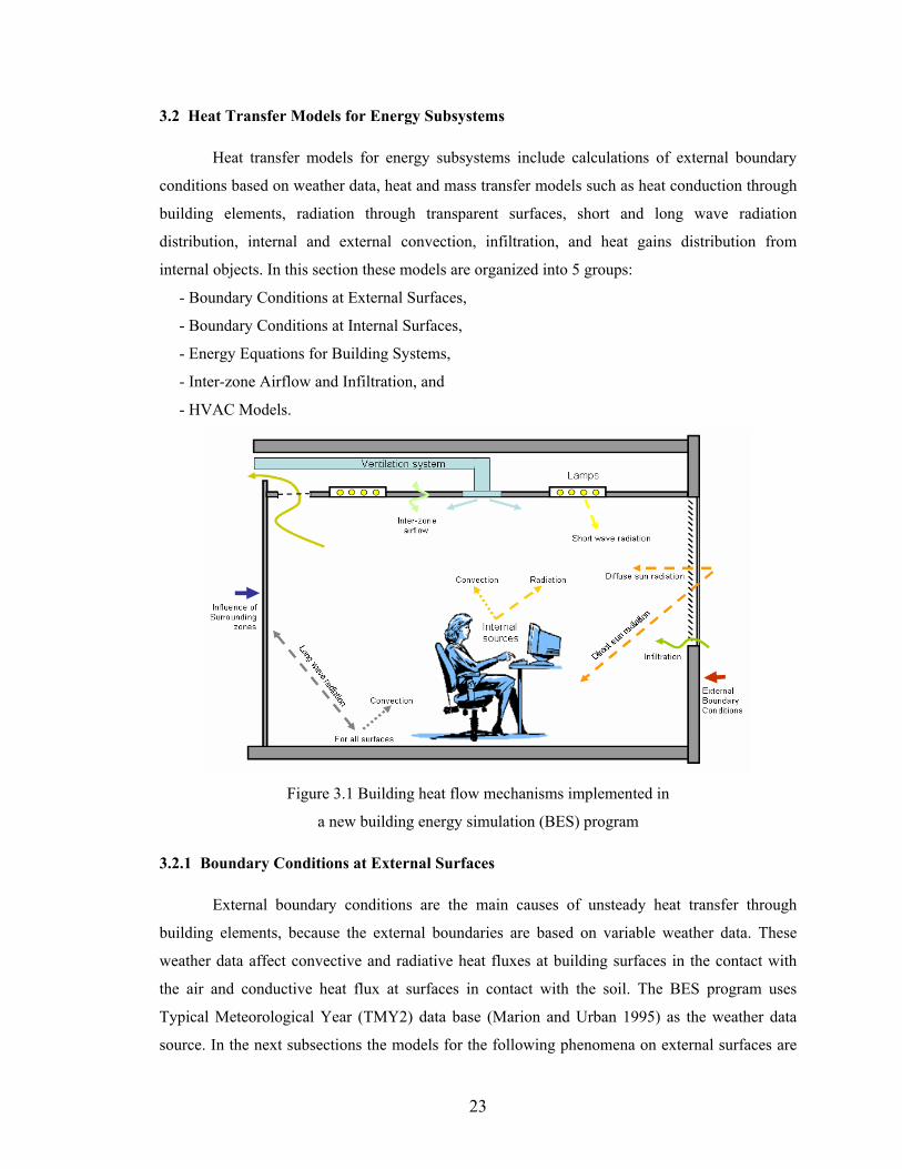
23

3.2 Heat Transfer Models for Energy Subsystems Heat transfer models for energy subsystems include calculations of external boundary

conditions based on weather data, heat and mass transfer models such as heat conduction through

building elements, radiation through transparent surfaces, short and long wave radiation

distribution, internal and external convection, infiltration, and heat gains distribution from

internal objects. In this section these models are organized into 5 groups:

- Boundary Conditions at External Surfaces,

- Boundary Conditions at Internal Surfaces,

- Energy Equations for Building Systems,

- Inter-zone Airflow and Infiltration, and

- HVAC Models.

Figure 3.1 Building heat flow mechanisms implemented in

a new building energy simulation (BES) program 3.2.1 Boundary Conditions at External Surfaces External boundary conditions are the main causes of unsteady heat transfer through

building elements, because the external boundaries are based on variable weather data. These

weather data affect convective and radiative heat fluxes at building surfaces in the contact with

the air and conductive heat flux at surfaces in contact with the soil. The BES program uses

Typical Meteorological Year (TMY2) data base (Marion and Urban 1995) as the weather data

source. In the next subsections the models for the following phenomena on external surfaces are

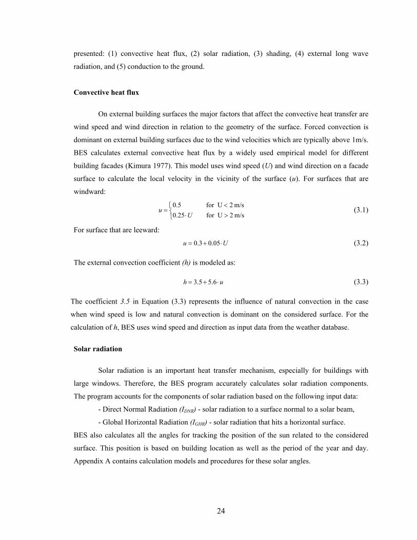
24

presented: (1) convective heat flux, (2) solar radiation, (3) shading, (4) external long wave

radiation, and (5) conduction to the ground.

Convective heat flux

On external building surfaces the major factors that affect the convective heat transfer are

wind speed and wind direction in relation to the geometry of the surface. Forced convection is

dominant on external building surfaces due to the wind velocities which are typically above 1m/s.

BES calculates external convective heat flux by a widely used empirical model for different

building facades (Kimura 1977). This model uses wind speed (U) and wind direction on a facade

surface to calculate the local velocity in the vicinity of the surface (u). For surfaces that are

windward:

m/s 2for U 0.25

m/s 2for U 0.5

>⋅<

=U

u (3.1)

For surface that are leeward:

05.03.0 Uu ⋅+= (3.2)

The external convection coefficient (h) is modeled as:

uh ⋅+= 6.55.3 (3.3)

The coefficient 3.5 in Equation (3.3) represents the influence of natural convection in the case

when wind speed is low and natural convection is dominant on the considered surface. For the

calculation of h, BES uses wind speed and direction as input data from the weather database.

Solar radiation

Solar radiation is an important heat transfer mechanism, especially for buildings with

large windows. Therefore, the BES program accurately calculates solar radiation components.

The program accounts for the components of solar radiation based on the following input data:

- Direct Normal Radiation (IDNR) - solar radiation to a surface normal to a solar beam,

- Global Horizontal Radiation (IGHR) - solar radiation that hits a horizontal surface.

BES also calculates all the angles for tracking the position of the sun related to the considered

surface. This position is based on building location as well as the period of the year and day.

Appendix A contains calculation models and procedures for these solar angles.

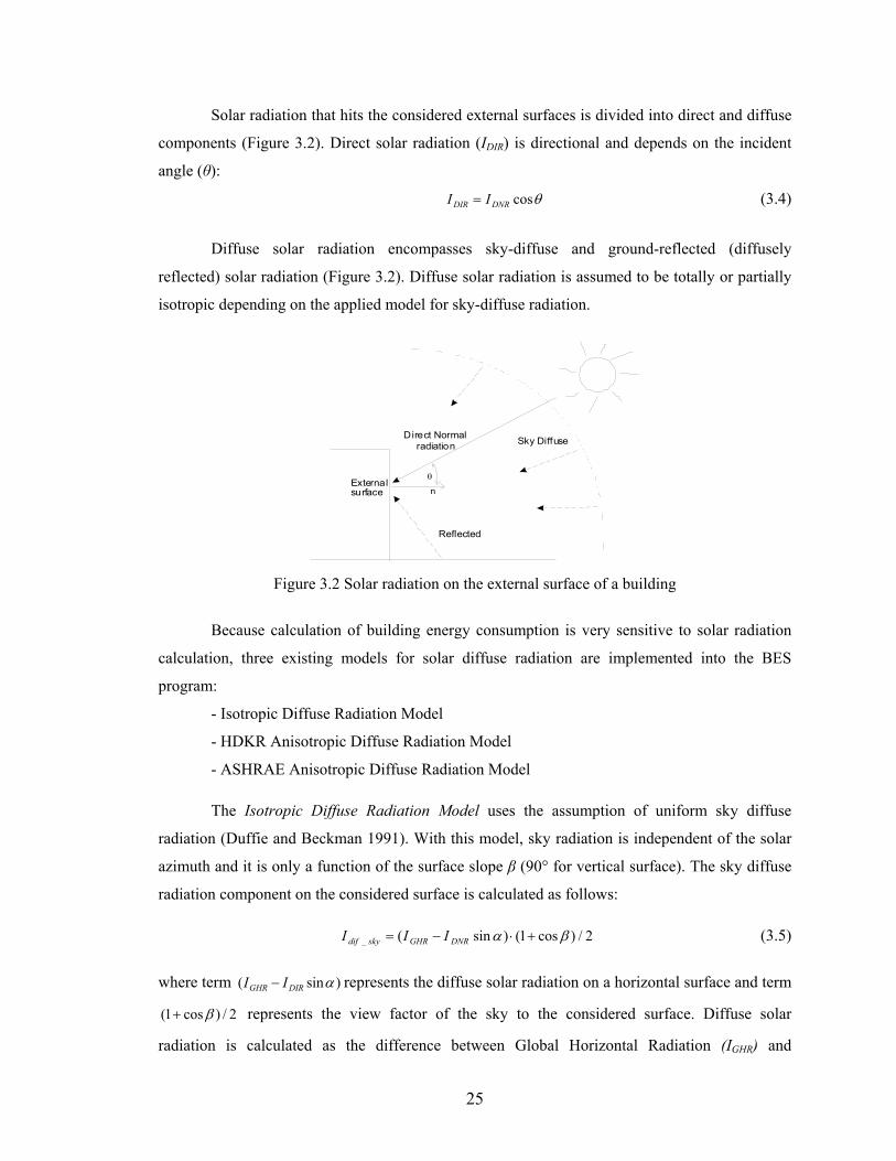
25

Solar radiation that hits the considered external surfaces is divided into direct and diffuse

components (Figure 3.2). Direct solar radiation (IDIR) is directional and depends on the incident

angle (θ):

θcosDNRDIR II = (3.4)

Diffuse solar radiation encompasses sky-diffuse and ground-reflected (diffusely

reflected) solar radiation (Figure 3.2). Diffuse solar radiation is assumed to be totally or partially

isotropic depending on the applied model for sky-diffuse radiation.

Externalsurface

Sky DiffuseDirect Normalradiation

Reflected

n

θ

Figure 3.2 Solar radiation on the external surface of a building

Because calculation of building energy consumption is very sensitive to solar radiation

calculation, three existing models for solar diffuse radiation are implemented into the BES

program:

- Isotropic Diffuse Radiation Model

- HDKR Anisotropic Diffuse Radiation Model

- ASHRAE Anisotropic Diffuse Radiation Model

The Isotropic Diffuse Radiation Model uses the assumption of uniform sky diffuse

radiation (Duffie and Beckman 1991). With this model, sky radiation is independent of the solar

azimuth and it is only a function of the surface slope β (90° for vertical surface). The sky diffuse

radiation component on the considered surface is calculated as follows:

2/)cos1()sin(_ βα +⋅−= DNRGHRskydif III (3.5)

where term )sin( αDIRGHR II − represents the diffuse solar radiation on a horizontal surface and term

2/)cos1( β+ represents the view factor of the sky to the considered surface. Diffuse solar

radiation is calculated as the difference between Global Horizontal Radiation (IGHR) and

26

orthogonal component of Direct Normal Radiation (IDIR). The angle α is solar altitude (see

Appendix A).

The HDKR Anisotropic Diffuse Radiation Model (Hay, Davies, Klucher, and Reindl

radiation model) is an anisotropic diffuse radiation model (Duffie and Beckman 1991). This

model corrects the Isotropic Diffuse Radiation Model for circumsolar diffuse radiation and

horizon brightening. The sky diffuse radiation component on a considered surface is calculated as

follows:

[ ]RAfAIII iiDIRGHRskydif ++⋅+⋅−⋅−= ))2/(sin1(2/)cos1()1()sin( 3_ ββα (3.6)

The equation terms (1-Ai) and (AiR) are for the correction for circumsolar diffuse radiation.

Coefficient R is the ratio between global radiation on considered surface and global horizontal

radiation. Anisotropy index Ai is a function of atmosphere transmittance, which is calculated as a

ratio between Direct Normal Radiation on the ground (IDIR_ground) and Direct Normal Radiation on

the outer layer of the atmosphere (IDIR_extraterrestrial):

strialextraterreDIRgroundDIRi IIA __ /= (3.7)

Term ))2/(sin1( 3 βf+ is the correction for horizon brightening where f is function of the ratio

between Direct Normal Radiation and Global Horizontal Radiation.

GHRDIR IIf /= (3.8)

The Anisotropic Diffuse Radiation Model presented by ASHRAE (ASHRAE

Fundamentals 2001) introduces a simpler correction method of the Isotropic Diffuse Radiation

Model that is valid only for vertical surfaces. Here, the sky diffuse radiation component on the

considered surface is calculated as follows:

YIII DIRGHRskydif ⋅−= )sin(_ α (3.9)

where coefficient Y represents the ratio of the sky diffuse radiation on a vertical surface to the sky

diffuse radiation on a horizontal surface. This coefficient is calculated as follows:

2.0cos for 4502.0cos for cos3130cos4370550 2

<=>⋅+⋅+=

θθ

.Y θ)(.θ. .Y (3.10)

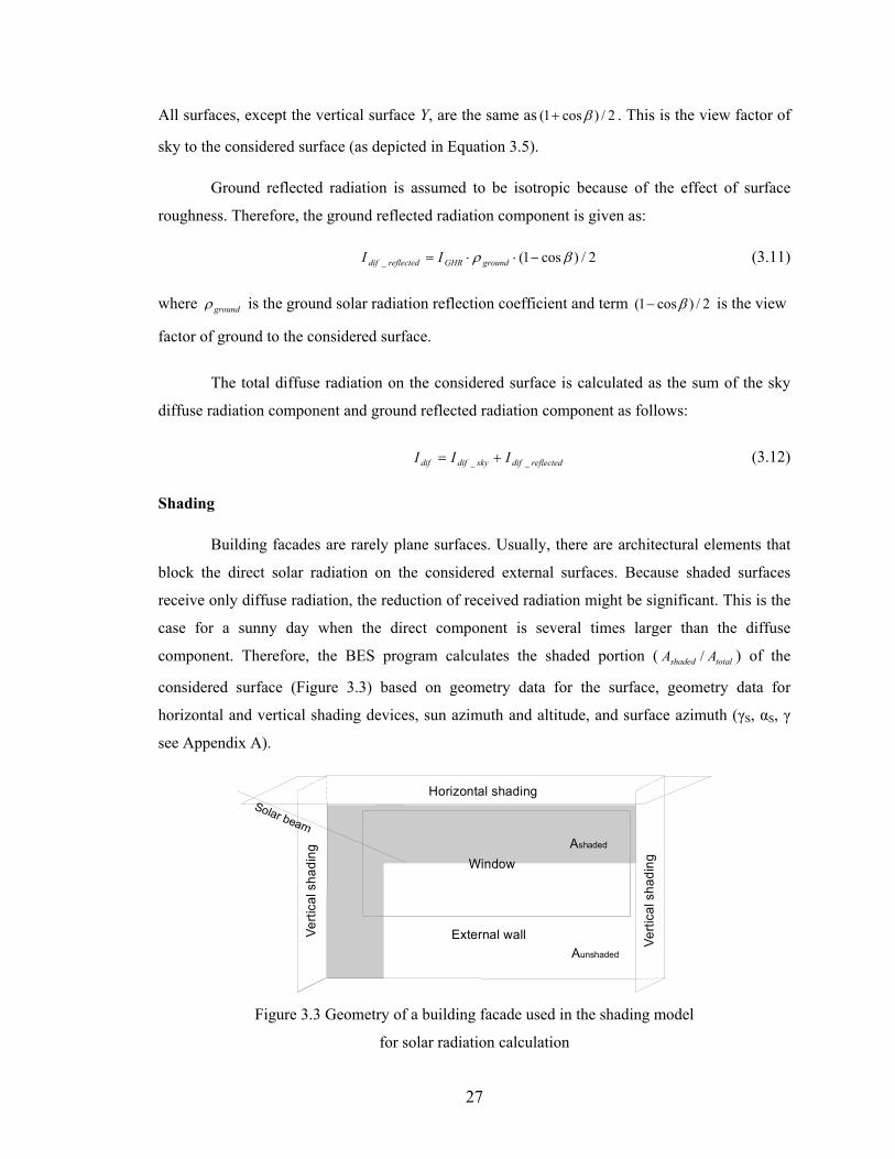
27

All surfaces, except the vertical surface Y, are the same as 2/)cos1( β+ . This is the view factor of

sky to the considered surface (as depicted in Equation 3.5). Ground reflected radiation is assumed to be isotropic because of the effect of surface

roughness. Therefore, the ground reflected radiation component is given as:

2/)cos1(_ βρ −⋅⋅= groundGHRreflecteddif II (3.11)

where groundρ is the ground solar radiation reflection coefficient and term 2/)cos1( β− is the view

factor of ground to the considered surface.

The total diffuse radiation on the considered surface is calculated as the sum of the sky

diffuse radiation component and ground reflected radiation component as follows:

reflecteddifskydifdif III __ += (3.12)

Shading Building facades are rarely plane surfaces. Usually, there are architectural elements that

block the direct solar radiation on the considered external surfaces. Because shaded surfaces

receive only diffuse radiation, the reduction of received radiation might be significant. This is the

case for a sunny day when the direct component is several times larger than the diffuse

component. Therefore, the BES program calculates the shaded portion ( totalshaded AA / ) of the

considered surface (Figure 3.3) based on geometry data for the surface, geometry data for

horizontal and vertical shading devices, sun azimuth and altitude, and surface azimuth (γS, αS, γ

see Appendix A).

Window

External wall

Horizontal shading

Verti

cal s

hadi

ng

Verti

cal s

hadi

ng

Ashaded

Aunshaded

Solar beam

Figure 3.3 Geometry of a building facade used in the shading model

for solar radiation calculation

28

Based on the shaded portion, diffuse (Idif), and direct (IDIR) components of solar radiation,

program calculates absorbed and, in the case of windows, the transmitted portion of the solar

radiation. For opaque surfaces, absorbed solar radiation is calculated as follows:

[ ]diftotalshadedDIRshortwaveSabsorbed IAAIq +−⋅⋅= )/1(_ α (3.13)

where αshortwave represents the absorption coefficient for shortwave radiation.

For windows, the transmitted portion of diffuse and direct radiation is calculated

separately because these two components of solar radiation are distributed inside the room in two

different ways. The details about transmitted direct and diffuse solar radiation in the room are

given in the following section that describes the distribution of short wave radiation in a room.

Direct solar radiation transmitted through windows is given as:

)/1(_ totalshadedDIRDIRDIRtransm AAIq −⋅⋅= τ (3.14)

where τDIR is the window transmittance coefficient for direct solar radiation. This coefficient

depends on the window structure and it is described in the following section that explains how

window models work. Windows transmitted diffuse radiation is given as:

difdifdiftransm Iq ⋅= τ_ (3.15)

where τdif is the window transmittances coefficient for direct solar radiation. This coefficient is

also described in the following section (Section 3.2.3).

External long wave radiation

External surfaces exchange energy with surrounding surfaces of different temperatures by

long-wave radiation. In the model used in the BES program, external surfaces “radiate” energy to

the sky and to the ground as illustrated in Figure 3.4.

External surface heat exchange with the ground is given as:

)(2/)cos1( 44_ groundsurfgroundsurfgroundsurf TTq −⋅⋅⋅−= εεσβ (3.16)

where (1-cosβ)/2 is the view factor, σ is the black body radiation constant, and ε is the emissivity

constant for the surface and ground. Because of the solution procedure, this radiative heat

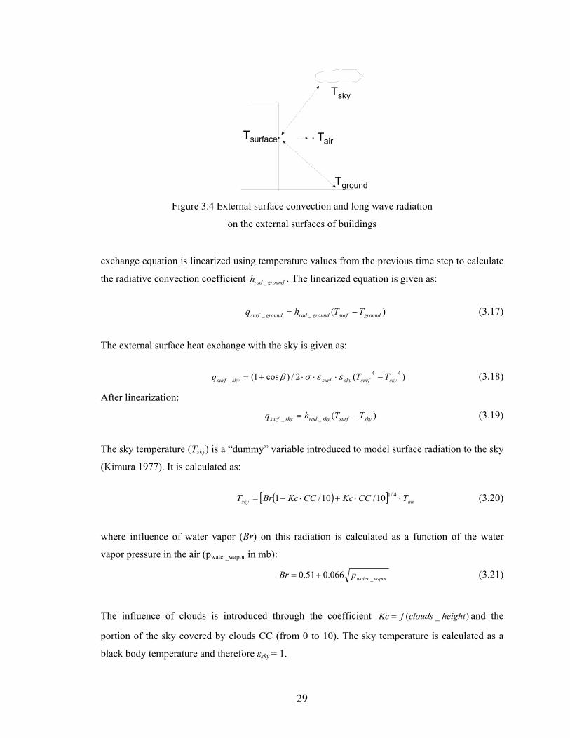
29

T ground

Tsurface Tair

Tsky

Figure 3.4 External surface convection and long wave radiation

on the external surfaces of buildings

exchange equation is linearized using temperature values from the previous time step to calculate

the radiative convection coefficient groundradh _ . The linearized equation is given as:

)(__ groundsurfgroundradgroundsurf TThq −= (3.17)

The external surface heat exchange with the sky is given as:

)(2/)cos1( 44

_ skysurfskysurfskysurf TTq −⋅⋅⋅+= εεσβ (3.18)

After linearization: )(__ skysurfskyradskysurf TThq −= (3.19)

The sky temperature (Tsky) is a “dummy” variable introduced to model surface radiation to the sky

(Kimura 1977). It is calculated as:

( )[ ] airsky TCCKcCCKcBrT ⋅⋅+⋅−= 4/110/10/1 (3.20)

where influence of water vapor (Br) on this radiation is calculated as a function of the water

vapor pressure in the air (pwater_wapor in mb):

vaporwaterpBr _066.051.0 += (3.21)

The influence of clouds is introduced through the coefficient )_( heightcloudsfKc = and the

portion of the sky covered by clouds CC (from 0 to 10). The sky temperature is calculated as a

black body temperature and therefore εsky = 1.

30

To calculate external long wave radiation, the model implemented into BES program

assumes that the ground surface temperature is equal to the air temperature. There is also an

option that users define this temperature. The sky temperature is calculated based on

meteorological data for cloud height, and the portion of the sky covered by clouds. Water vapor

pressure needed for the sky temperature calculation (Equations 3.20 and 3.21) is calculated using

relative humidity and the dry bulb temperature from weather data base. Conduction to the ground

For an external surface that is in contact with the ground, the BES program uses the

simplified model, which is given as:

)(/_ groundSgroundgroundcond TTLkq −⋅= (3.22)

Based on the location of the ground configuration, the user defines the ground temperature

(Tground) at distance (L) and ground conductivity (kground). The user may improve this model by

providing the seasonal changes of ground temperatures.

3.2.2 Boundary Conditions at Internal Surfaces

In the next subsections the models for the following heat transfer mechanisms at internal

surfaces are presented:

(1) convection,

(2) long wave radiation,

(3) short wave radiation.

Convection

Convection coefficients used in the BES program are calculated based on expressions for

mixed convection provided by Beausoleil (2000). He created this correlation by combining the

correlations for natural convection (Alamdari and Hammond 1983) and for forced convection

where the air is supplied by a ceiling diffuser (Fisher 1995). For vertical surfaces, the program

calculates convection coefficients for forced and natural convections (hf and hn). Depending on

the air movement created by forced and natural convection (opposing or assisting), the BES

program uses the appropriate model to combine these two heat transfer mechanisms (Table 3.1).

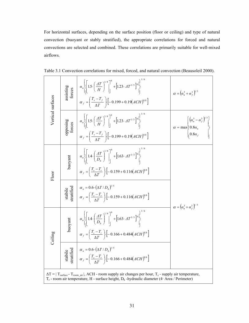
31

For horizontal surfaces, depending on the surface position (floor or ceiling) and type of natural

convection (buoyant or stably stratified), the appropriate correlations for forced and natural

convections are selected and combined. These correlations are primarily suitable for well-mixed

airflows.

Table 3.1 Convection correlations for mixed, forced, and natural convection (Beausoleil 2000). as

sist

ing

forc

es [ ]

6/1

6 31

641

23151

⋅+

⋅ /

/

n ∆T.H∆T.α

( )[ ]8.019.0199.0 ACHTTT fs

f +−⋅

∆

−=α

( ) 3/133fn αα +=α

Ver

tical

surf

aces

oppo

sing

fo

rces

[ ]6/1

6 31

641

23151

⋅+

⋅ /

/

n ∆T.H∆T.α

( )[ ]8.019.0199.0 ACHTTT fs

f +−⋅

∆

−=α

( )

−

=

f

n

fn

α

α

αα

8.0

8.0max

3/133

α

buoy

ant [ ]

6/1

6 31

641

63141

⋅+

⋅ /

/

hn ∆T.

D∆T.α

( )[ ]8.0116.0159.0 ACHTTT rs

f +−⋅

∆−

=α

Floo

r

stab

ile

stra

tifie

d ( ) 5/1/6.0 hn DT∆⋅=α ( )[ ]8.0116.0159.0 ACH

TTT rs

f +−⋅

∆−

=α

buoy

ant [ ]

6/1

6 31

641

63141

⋅+

⋅ /

/

hn ∆T.

D∆T.α

( )[ ]8.0484.0166.0 ACHTTT rs

f +−⋅

∆−

=α

Cei

ling

stab

ile

stra

tifie

d ( ) 5/1/6.0 hn DT∆⋅=α

( )[ ]8.0484.0166.0 ACHTTT rs

f +−⋅

∆−

=α

( ) 3/133fn αα +=α

∆T = | Tsurface - Troom_air |, ACH - room supply air changes per hour, Ts - supply air temperature, Tr - room air temperature, H - surface height, Dh -hydraulic diameter (4· Area / Perimeter)

32

Long wave radiation

Internal surfaces with different temperatures exchange energy through long wave

radiation. To calculate the relevant radiative heat fluxes, view factors between all pairs of

surfaces are required. The view factor of surface ‘i’ to surface ‘j’ is calculated by the following

equation:

∫ ∫⋅

=i jA A

jiji

iij dAdA

sAF 2

coscos1π

ϕϕ (3.23)

All internal surfaces used in the BES program are parallel or orthogonal to each other. Therefore,

only two characteristic solutions of equation (3.23) are used in BES (Fij_parale and Fij_ortogonal).

Detailed expressions for the view factors are given in Appendix B. Using these expressions and

room geometry, the program calculates view factors for all surfaces by creating a matrix [n×n],

where n is total number of surfaces. The room surfaces form a closed environment and therefore:

∑=

==++++n

jijiniii FFFFF

1321 1... ni ,...,2,1= (3.24)

Long wave radiative heat flux at surface (q) may be determined by using the radiosity

method (ASHRAE Fundamentals 2001). Radiosity (J) is the total energy that is emitted and

reflected from a surface. It is calculated using the system of equations given by:

∑=

−+=n

jiijiiii JFTJ

1

4 )1( εσε ni ,...,2,1= (3.25)

The radiative heat flux that surface ‘i’ receives is given as:

ii

iii

JTqεε

σ/)1(

4

−−

= (3.26)

This radiosity method creates a system of equations dependent on fourth power of

temperature. Combining these equations with the linear temperature equations creates a system of

linear and highly nonlinear equations that is difficult to solve. Therefore, instead of using the

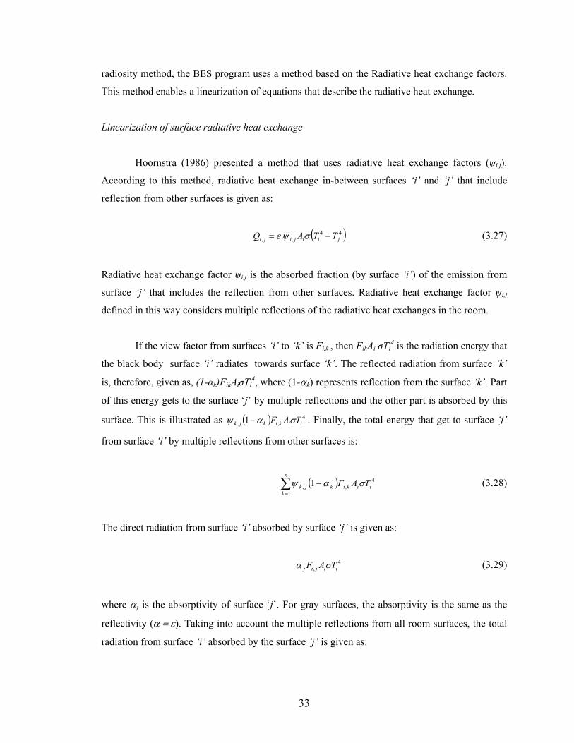
33

radiosity method, the BES program uses a method based on the Radiative heat exchange factors.

This method enables a linearization of equations that describe the radiative heat exchange.

Linearization of surface radiative heat exchange

Hoornstra (1986) presented a method that uses radiative heat exchange factors (ψi,j).

According to this method, radiative heat exchange in-between surfaces ‘i’ and ‘j’ that include

reflection from other surfaces is given as:

( )44,, jiijiiji TTAQ −= σψε (3.27)

Radiative heat exchange factor ψi,j is the absorbed fraction (by surface ‘i’) of the emission from

surface ‘j’ that includes the reflection from other surfaces. Radiative heat exchange factor ψi,j

defined in this way considers multiple reflections of the radiative heat exchanges in the room.

If the view factor from surfaces ‘i’ to ‘k’ is Fi,k , then FikAi σTi4 is the radiation energy that

the black body surface ‘i’ radiates towards surface ‘k’. The reflected radiation from surface ‘k’

is, therefore, given as, (1-αk)FikAiσTi4, where (1-αk) represents reflection from the surface ‘k’. Part

of this energy gets to the surface ‘j’ by multiple reflections and the other part is absorbed by this

surface. This is illustrated as ( ) 4,, 1 iikikjk TAF σαψ − . Finally, the total energy that get to surface ‘j’

from surface ‘i’ by multiple reflections from other surfaces is:

( )∑=

−n

kiikikjk TAF

1

4,, 1 σαψ (3.28)

The direct radiation from surface ‘i’ absorbed by surface ‘j’ is given as:

4

, iijij TAF σα (3.29)

where αj is the absorptivity of surface ‘j’. For gray surfaces, the absorptivity is the same as the

reflectivity (α = ε). Taking into account the multiple reflections from all room surfaces, the total

radiation from surface ‘i’ absorbed by the surface ‘j’ is given as:

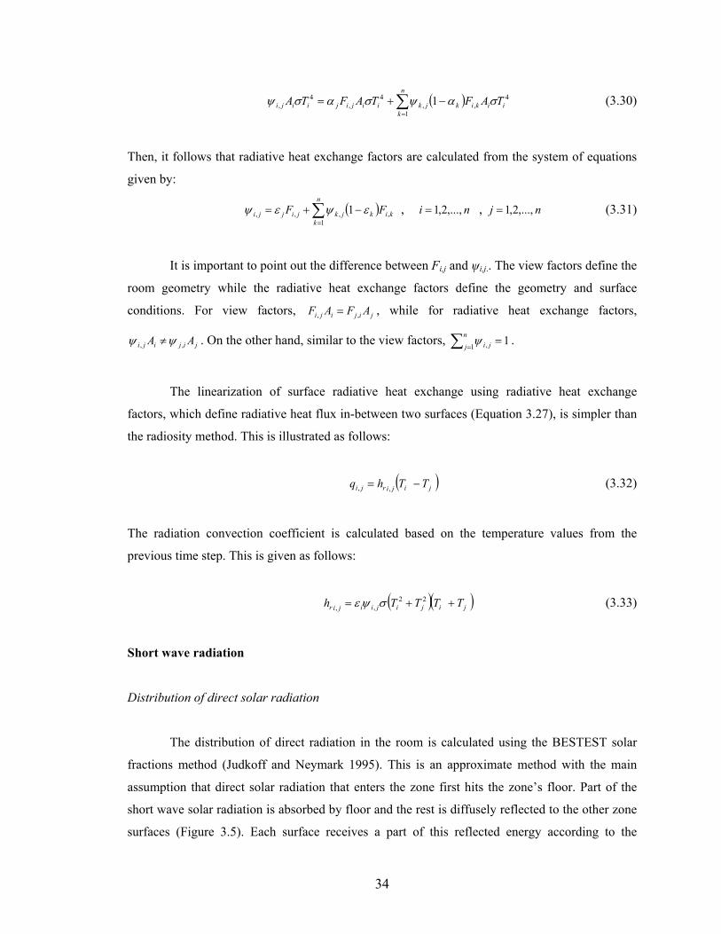
34

( )∑=

−+=n

kiikikjkiijijiiji TAFTAFTA

1

4,,

4,

4, 1 σαψσασψ (3.30)

Then, it follows that radiative heat exchange factors are calculated from the system of equations

given by:

( )∑=

−+=n

kkikjkjijji FF

1,,,, 1 εψεψ , ni ,...,2,1= , nj ,...,2,1= (3.31)

It is important to point out the difference between Fi,j and ψi,j.. The view factors define the

room geometry while the radiative heat exchange factors define the geometry and surface

conditions. For view factors, jijiji AFAF ,, = , while for radiative heat exchange factors,

jijiji AA ,, ψψ ≠ . On the other hand, similar to the view factors, 11 , =∑ =

n

j jiψ .

The linearization of surface radiative heat exchange using radiative heat exchange

factors, which define radiative heat flux in-between two surfaces (Equation 3.27), is simpler than

the radiosity method. This is illustrated as follows:

( )jijirji TThq −= ,, (3.32)

The radiation convection coefficient is calculated based on the temperature values from the

previous time step. This is given as follows:

( )( )jijijiijir TTTTh ++= 22,, σψε (3.33)

Short wave radiation

Distribution of direct solar radiation

The distribution of direct radiation in the room is calculated using the BESTEST solar

fractions method (Judkoff and Neymark 1995). This is an approximate method with the main

assumption that direct solar radiation that enters the zone first hits the zone’s floor. Part of the

short wave solar radiation is absorbed by floor and the rest is diffusely reflected to the other zone

surfaces (Figure 3.5). Each surface receives a part of this reflected energy according to the

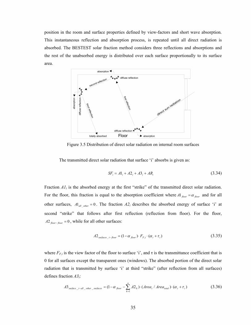
35

position in the room and surface properties defined by view-factors and short wave absorption.

This instantaneous reflection and absorption process, is repeated until all direct radiation is

absorbed. The BESTEST solar fraction method considers three reflections and absorptions and

the rest of the unabsorbed energy is distributed over each surface proportionally to its surface

area.

diffuse reflection

first reflection

third reflection

second reflection

Floor absorption

absorption ab

sorp

tion

diffuse reflectiondi

ffuse

refle

ctio

n

totally absorbed Figure 3.5 Distribution of direct solar radiation on internal room surfaces

The transmitted direct solar radiation that surface ‘i’ absorbs is given as:

iiiii ARAAASF +++= 321 (3.34)

Fraction A1i is the absorbed energy at the first “strike” of the transmitted direct solar radiation.

For the floor, this fraction is equal to the absorption coefficient where floorfloorA α=1 and for all

other surfaces, 01 _ =otherallA . The fraction A2i describes the absorbed energy of surface ‘i’ at

second “strike” that follows after first reflection (reflection from floor). For the floor,

02 =− floorfloorA , while for all other surfaces:

)()1(2 ,_ iiiFfloorfloorisurfaces FA ταα +⋅⋅−=− (3.35)

where FF,i is the view factor of the floor to surface ‘i’, and τ is the transmittance coefficient that is

0 for all surfaces except the transparent ones (windows). The absorbed portion of the direct solar

radiation that is transmitted by surface ‘i’ at third “strike” (after reflection from all surfaces)

defines fraction A3i:

)()/()21(31

___ iitotali

n

kkfloorsurfacesotherallisurface AreaAreaAA ταα +⋅⋅−−= ∑

=− (3.36)

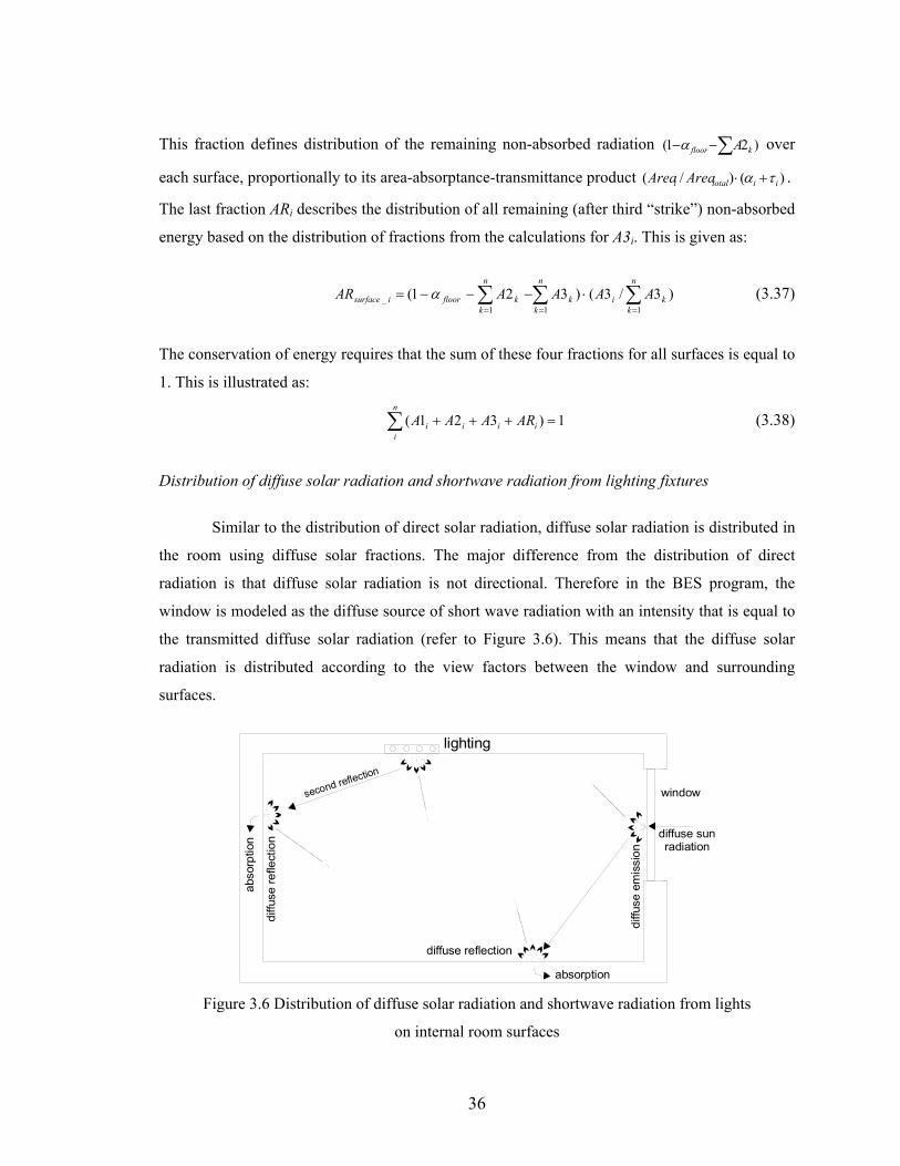
36

This fraction defines distribution of the remaining non-absorbed radiation )21( ∑−− kfloor Aα over

each surface, proportionally to its area-absorptance-transmittance product )()/( iitotali AreaArea τα +⋅ .

The last fraction ARi describes the distribution of all remaining (after third “strike”) non-absorbed

energy based on the distribution of fractions from the calculations for A3i. This is given as:

)3/3()321(111

_ ∑∑∑===

⋅−−−=n

kki

n

kk

n

kkfloorisurface AAAAAR α (3.37)

The conservation of energy requires that the sum of these four fractions for all surfaces is equal to

1. This is illustrated as:

1)321( =+++∑n

iiiii ARAAA (3.38)

Distribution of diffuse solar radiation and shortwave radiation from lighting fixtures

Similar to the distribution of direct solar radiation, diffuse solar radiation is distributed in

the room using diffuse solar fractions. The major difference from the distribution of direct

radiation is that diffuse solar radiation is not directional. Therefore in the BES program, the

window is modeled as the diffuse source of short wave radiation with an intensity that is equal to

the transmitted diffuse solar radiation (refer to Figure 3.6). This means that the diffuse solar

radiation is distributed according to the view factors between the window and surrounding

surfaces.

diffuse sunradiation

second reflection

absorption

abso

rptio

n

lighting

window

diffu

se e

mis

sion

diffuse reflection

diffu

se re

flect

ion

Figure 3.6 Distribution of diffuse solar radiation and shortwave radiation from lights

on internal room surfaces

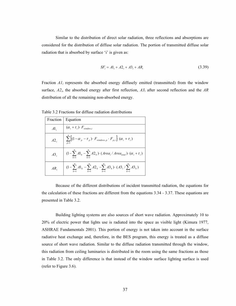
37

Similar to the distribution of direct solar radiation, three reflections and absorptions are

considered for the distribution of diffuse solar radiation. The portion of transmitted diffuse solar

radiation that is absorbed by surface ‘i’ is given as:

iiiii ARAAASF +++= 321 (3.39)

Fraction A1i represents the absorbed energy diffusely emitted (transmitted) from the window

surface, A2i, the absorbed energy after first reflection, A3i after second reflection and the AR

distribution of all the remaining non-absorbed energy.

Table 3.2 Fractions for diffuse radiation distributions

Fraction Equation

iA1 iwindowii F ,)( ⋅+τα

iA2 [ ] )()1(1

,, ii

n

pippwindowspp FF τατα +⋅⋅⋅−−∑

=

iA3 )()/()211(11

iitotali

n

kk

n

kk AreaAreaAA τα +⋅⋅−− ∑∑

==

iAR )3/3()3211(1111

∑∑∑∑====

⋅−−−n

kki

n

kk

n

kk

n

kk AAAAA

Because of the different distributions of incident transmitted radiation, the equations for

the calculation of these fractions are different from the equations 3.34 - 3.37. These equations are

presented in Table 3.2.

Building lighting systems are also sources of short wave radiation. Approximately 10 to

20% of electric power that lights use is radiated into the space as visible light (Kimura 1977,

ASHRAE Fundamentals 2001). This portion of energy is not taken into account in the surface

radiative heat exchange and, therefore, in the BES program, this energy is treated as a diffuse

source of short wave radiation. Similar to the diffuse radiation transmitted through the window,

this radiation from ceiling luminaries is distributed in the room using the same fractions as those

in Table 3.2. The only difference is that instead of the window surface lighting surface is used

(refer to Figure 3.6).

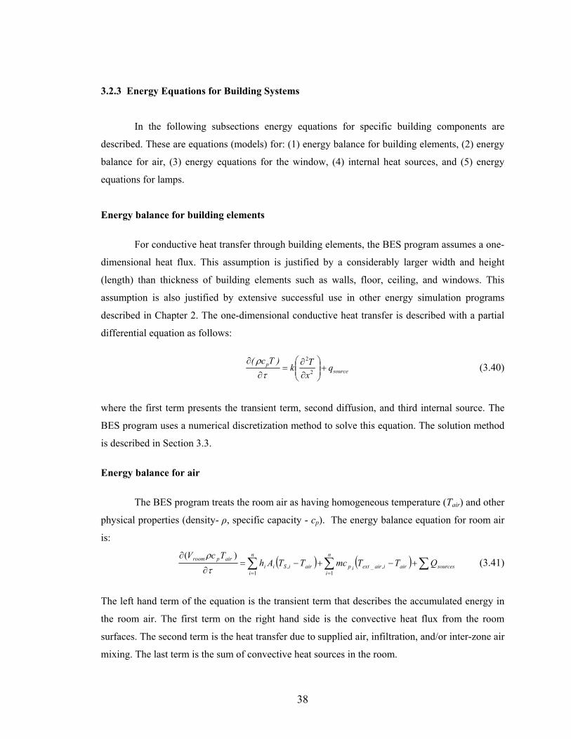
38

3.2.3 Energy Equations for Building Systems

In the following subsections energy equations for specific building components are

described. These are equations (models) for: (1) energy balance for building elements, (2) energy

balance for air, (3) energy equations for the window, (4) internal heat sources, and (5) energy

equations for lamps.

Energy balance for building elements

For conductive heat transfer through building elements, the BES program assumes a one-

dimensional heat flux. This assumption is justified by a considerably larger width and height

(length) than thickness of building elements such as walls, floor, ceiling, and windows. This

assumption is also justified by extensive successful use in other energy simulation programs

described in Chapter 2. The one-dimensional conductive heat transfer is described with a partial

differential equation as follows:

sourcep q

xTk

)Tc(+

∂∂

=∂

∂2

2

τρ

(3.40)

where the first term presents the transient term, second diffusion, and third internal source. The

BES program uses a numerical discretization method to solve this equation. The solution method

is described in Section 3.3. Energy balance for air

The BES program treats the room air as having homogeneous temperature (Tair) and other

physical properties (density- ρ, specific capacity - cp). The energy balance equation for room air

is:

( ) ( ) ∑∑∑ +−+−=∂

∂

==sources

n

iairiairextip

n

iairiSii

airproom QTTmcTTAhTcV

1,_

1,

)(τρ

(3.41)

The left hand term of the equation is the transient term that describes the accumulated energy in

the room air. The first term on the right hand side is the convective heat flux from the room

surfaces. The second term is the heat transfer due to supplied air, infiltration, and/or inter-zone air

mixing. The last term is the sum of convective heat sources in the room.

39

Energy equations for the window

Heat transfer through the window structure is a complex process. For multiple glazing

windows, this process involves conduction, convection, and long wave radiation. Also, through

window surfaces, short wave solar radiation gets into the room. This transmitted solar radiation is

usually the major source of unsteady heat transfer in building elements. Therefore, a detailed

window model is developed for the BES program. A portion of the absorbed (α), transmitted (τ), and reflected (ρ) direct solar radiation that

hits the window glazing is a function of the incident angle θ (refer to Figure 3.7). The parameters

α, τ, and ρ are also functions of window glazing properties. However, α, τ, and ρ values for

diffuse solar radiation only depends on surface glazing properties. Therefore, these coefficients

are defined separately for direct and diffuse solar radiation.

τ

1

ρ α

θn

α + ρ + τ = 1

Figure 3.7 Transmission, absorption, and reflection on internal surfaces

For the calculation of the absorption (α) and transmission (τ) coefficients for diffuse (Idif)

and direct (IDIR) solar radiation, the window model uses following expressions:

∑=

=5

0cos

i

iiDIR ts θτ , ( )∑

=

+=5

02/2

iidif itsτ , ∑

=

=5

0cos

i

iiDIR as θα , ∑

=

+=5

0)2/(2

iidif iasα

(3.42)

The coefficients tsi and asi are constants which define glazing properties. In the BES program the

coefficients for “one-eighth-inch, clear double-strength glass” (ASHRAE 2001) are used as the

default.

For the double glazed window (refer to Figure 3.8), the overall transitivity and

absorbtivity for each layer needs to be calculated. Figure 3.8-a shows the multiple repetitions of

transmission, absorption and reflection. These repetitions can be expressed as a sum of an infinite

series to calculate the overall transitivity (Kimura 1977) as follows:

21

2122

212121212112 1

...ρρ

ττρρττρρτττττ−

=+++= (3.43)

40

The same approach is used for the calculation of the overall absorption coefficient of external

(α1_overall) and internal (α2_overall) glazing units as follows:

−

+=21

211_1 1

1ρρ

ρταα overall , 21

21_2 1 ρρ

ατα−

=overall (3.44)

The conductive heat flux for a single glazed window is described with equation (3.40),

where the absorbed solar radiation presents the source term. For the double glazed window, the

calculation of conductive heat flux includes conduction through glazing units, convection in

windows cavity and long wave radiation in-between glazing surfaces (Figure 3.8).

1

τ1

τ1τ

2

τ1 1ρ τ ρ

2 2

τ1 1

2

ρ τ ρ2 2

2

τ1 1

2

ρ τ ρ2 2

2

τ1 1

2

ρ τ2

τ1ρ ρ

1 2

2

τ1

2

ρ2

τ1ρ

2

1 2

τ1ρ ρ

1 2

ρ1

α1

α1

τ ρ α1 2 1

τ α1 2

τ ρ ρ α1 1 2 2

1

τ1

τ1τ

2

τ1 1ρ τ ρ

2 2

τ1 1

2

ρ τ ρ2 2

2

τ1 1

2

ρ τ ρ2 2

2

τ1 1

2

ρ τ2

τ1ρ ρ

1 2

2

τ1

2

ρ2

τ1ρ

2

1 2

τ1ρ ρ

1 2

ρ1

α1

α1

τ ρ α1 2 1

τ α1 2

τ ρ ρ α1 1 2 2

1 2

α2

α1

exte

rnal

sur

face

s

inte

rnal

sur

face

s

mutual radiation

1 2

internal air

external air

windowcavity

air

c) Convectionb) Long-wave radiationa) Short-wave radiation Figure 3.8 Heat transfer for a double glazed window implemented into the BES program

To predict the temperature of glazing surfaces, air-cavity convection and long-wave

radiation heat fluxes need to be calculated. Radiative heat flux is calculated using a linearized

radiation convection coefficient (Equation 3.32). The convective heat flux is calculated by

convective model for Insulated Glazing Units (IGU) developed by Yin (Curcija 1992) as follows:

tl

kNuq

IGU

aircavityIGU ∆= _ (3.45)

The Nusselt number (Nu) is calculated based on the Grashof number (Gr), window cavity height

(h), and thickness of the cavity (lIGU) as follows:

131.0269.0 )/(21.0 −⋅= IGUlhGrNu (3.46)

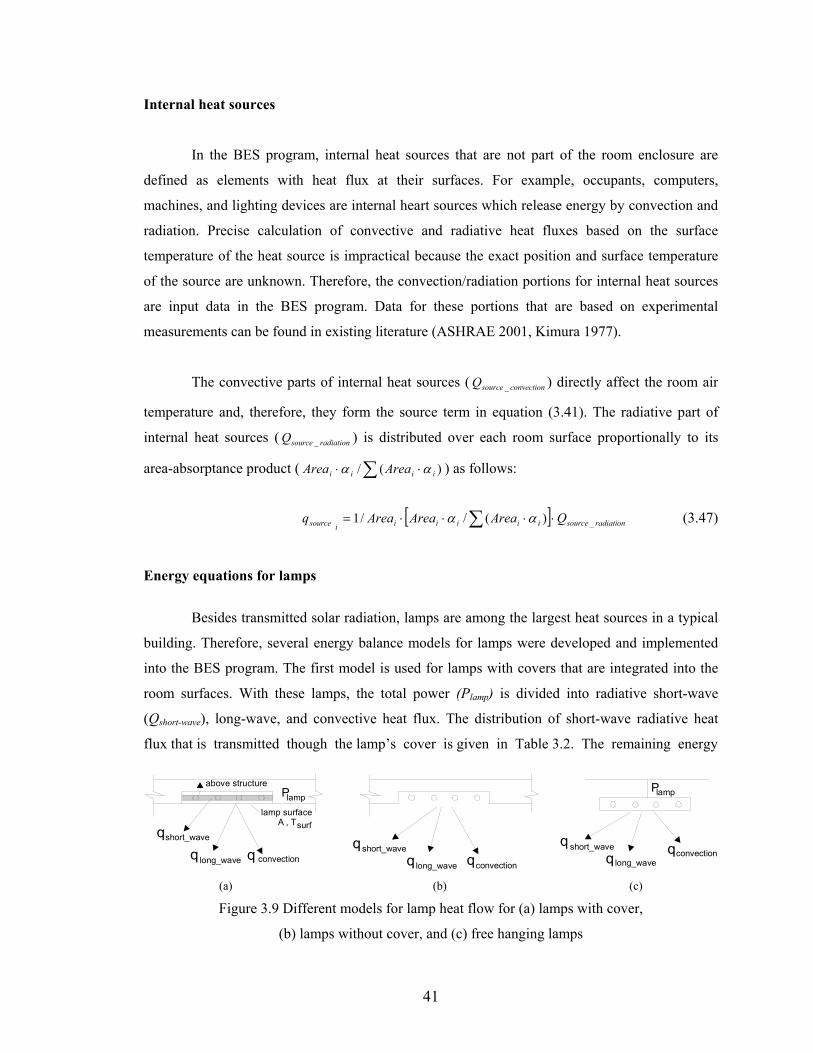
41

Internal heat sources

In the BES program, internal heat sources that are not part of the room enclosure are

defined as elements with heat flux at their surfaces. For example, occupants, computers,

machines, and lighting devices are internal heart sources which release energy by convection and

radiation. Precise calculation of convective and radiative heat fluxes based on the surface

temperature of the heat source is impractical because the exact position and surface temperature

of the source are unknown. Therefore, the convection/radiation portions for internal heat sources

are input data in the BES program. Data for these portions that are based on experimental

measurements can be found in existing literature (ASHRAE 2001, Kimura 1977).

The convective parts of internal heat sources ( convectionsourceQ _ ) directly affect the room air

temperature and, therefore, they form the source term in equation (3.41). The radiative part of

internal heat sources ( radiationsourceQ _ ) is distributed over each room surface proportionally to its

area-absorptance product ( ∑ ⋅⋅ )(/ iiii AreaArea αα ) as follows:

[ ] radiationsourceiiiiiisource QAreaAreaAreaq _)(//1 ⋅⋅⋅⋅= ∑ αα (3.47)

Energy equations for lamps

Besides transmitted solar radiation, lamps are among the largest heat sources in a typical

building. Therefore, several energy balance models for lamps were developed and implemented

into the BES program. The first model is used for lamps with covers that are integrated into the

room surfaces. With these lamps, the total power (Plamp) is divided into radiative short-wave

(Qshort-wave), long-wave, and convective heat flux. The distribution of short-wave radiative heat

flux that is transmitted though the lamp’s cover is given in Table 3.2. The remaining energy

above structure

lamp surface A , T

q

q q

P

q q

surf

q qlong_wave

q short_waveq

lamp

convection

short_wave

long_waveconvection

Plamp

convectionlong_wave

short_wave

(a) (b) (c)

Figure 3.9 Different models for lamp heat flow for (a) lamps with cover,

(b) lamps without cover, and (c) free hanging lamps

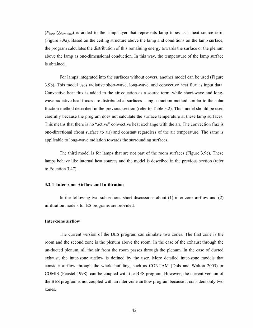
42

(Plamp-Qshort-wave) is added to the lamp layer that represents lamp tubes as a heat source term

(Figure 3.9a). Based on the ceiling structure above the lamp and conditions on the lamp surface,

the program calculates the distribution of this remaining energy towards the surface or the plenum

above the lamp as one-dimensional conduction. In this way, the temperature of the lamp surface

is obtained.

For lamps integrated into the surfaces without covers, another model can be used (Figure

3.9b). This model uses radiative short-wave, long-wave, and convective heat flux as input data.

Convective heat flux is added to the air equation as a source term, while short-wave and long-

wave radiative heat fluxes are distributed at surfaces using a fraction method similar to the solar

fraction method described in the previous section (refer to Table 3.2). This model should be used

carefully because the program does not calculate the surface temperature at these lamp surfaces.

This means that there is no “active” convective heat exchange with the air. The convection flux is

one-directional (from surface to air) and constant regardless of the air temperature. The same is

applicable to long-wave radiation towards the surrounding surfaces.

The third model is for lamps that are not part of the room surfaces (Figure 3.9c). These

lamps behave like internal heat sources and the model is described in the previous section (refer

to Equation 3.47).

3.2.4 Inter-zone Airflow and Infiltration

In the following two subsections short discussions about (1) inter-zone airflow and (2)

infiltration models for ES programs are provided.

Inter-zone airflow

The current version of the BES program can simulate two zones. The first zone is the

room and the second zone is the plenum above the room. In the case of the exhaust through the

un-ducted plenum, all the air from the room passes through the plenum. In the case of ducted

exhaust, the inter-zone airflow is defined by the user. More detailed inter-zone models that

consider airflow through the whole building, such as CONTAM (Dols and Walton 2003) or

COMIS (Feustel 1998), can be coupled with the BES program. However, the current version of

the BES program is not coupled with an inter-zone airflow program because it considers only two

zones.

43

Infiltration

The infiltration of outdoor air depends on the geometry of the whole building and on the

inter-zone airflow. Therefore, the infiltration in large buildings should be calculated using multu-

zone airflow programs. Because the BES program considers only one room with or without

plenum, the current version of the program offers the choice to the user to define the constant

infiltration rate or to select a simple model for infiltration in residential buildings (ASHRAE

2001).

This infiltration model considers buildings as a single zone and uses a superposition of

wind and stack effects. The infiltration mass flow rate is given as:

2

1000UCtC

Am wS

Lair +∆= ρ (3.48)

where AL is the effective air leakage area in cm2, Cs is stack coefficient, ∆t is temperature

difference between the room and outdoor air, Cw is the wind coefficient, and U is the wind speed.

The stack and wind coefficients are provided by the user based on building height and shelter

class information (ASHRAE 2001). For wind speeds and external temperatures, the BES program

uses meteorological data for each time step, while effective leakage area is a property of the

openings and it is defined as input data.

3.2.5 HVAC Models

The current version of the BES program has models for several HVAC configurations.

The primary purpose of integrated HVAC models is to demonstrate the performance of developed

methods for simultaneous load calculation and HVAC performance simulation. The selection of

integrated HVAC models is performed in such a way that all characteristic types of control

systems are present:

1) HVAC systems that control the room temperature, using the flow rate of supply air

(Vsupply), are represented by the Variable Air Volume (VAV) system for a single zone.

2) HVAC systems that use variable supply air temperature (Tsupply) for control are

represented by the Constant Air Volume (CAV) system.

3) Systems that use HVAC device surface temperature (Tsurface) to control the

environment temperature are presented by the radiant panel system.

44

4) Pure convective HVAC systems, which have negligible radiative heat exchange with

room surfaces and exchange energy with air directly by convection (Qconvective), are

represented by fan-coil and baseboard heater systems.

Surface temperature (Tsurface) and convective heat flux (Qconvective) of HVAC device are regulated

by temperature of fluid that circulates through the device. However, for linking of the HVAC

model with the building load calculation model, Tsurface and Qconvective are used. Details about this

linking are given in Section 3.4. The circulating-fluid temperature that is needed for providing

certain values of Tsurface or Qconvective is calculated in HVAC models.

Models of the HVAC system implemented into the BES program were developed for

steady state condition. Energy accumulation in HVAC components is not considered because it is

significantly smaller than energy accumulation in the building structure. The implemented HVAC

components are: radiant panels, fan coils, baseboard heaters and elements of simple air handling

units.

All-Air systems

The configurations of the Air Handling Unit (AHU) for VAV and CAV systems are the

same (Figure 3.10). The reason is that only single zones are analyzed and, therefore, there are

neither zone reheaters nor VAV boxes. The only difference lies in the control parameter. For

VAV, it is the supply air volume flow rate, while for CAV, it is the supply air temperature.

rmS fanscooler heater

mS

QC QH

wO wS

TR

room TR

Qroom_sensibel

(1-r)mS mS

wM

wR

Qroom_latent

TSTO

wR

TM

Tf,in Tf,out

Figure 3.10 Schematic for a model of a simple air handling unit

The VAV and CAV are modeled with equations that describe energy, air-mass, and air-

humidity balances for each component of the air handling units. In this model, the cooling load is

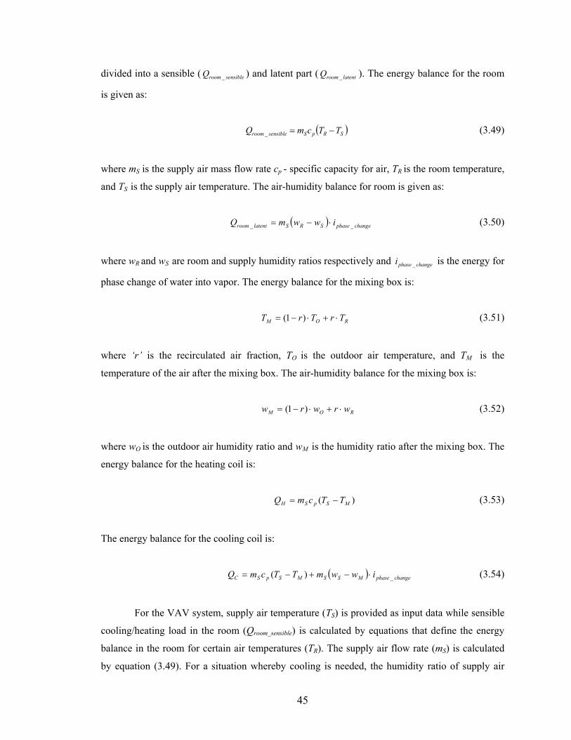
45

divided into a sensible ( sensibleroomQ _ ) and latent part ( latentroomQ _ ). The energy balance for the room

is given as:

( )SRpSsensibleroom TTcmQ −=_ (3.49)

where mS is the supply air mass flow rate cp - specific capacity for air, TR is the room temperature,

and TS is the supply air temperature. The air-humidity balance for room is given as:

( ) changephaseSRSlatentroom iwwmQ __ ⋅−= (3.50)

where wR and wS are room and supply humidity ratios respectively and changephasei _ is the energy for

phase change of water into vapor. The energy balance for the mixing box is:

ROM TrTrT ⋅+⋅−= )1( (3.51)

where ‘r’ is the recirculated air fraction, TO is the outdoor air temperature, and TM is the

temperature of the air after the mixing box. The air-humidity balance for the mixing box is:

ROM wrwrw ⋅+⋅−= )1( (3.52)

where wO is the outdoor air humidity ratio and wM is the humidity ratio after the mixing box. The

energy balance for the heating coil is:

)( MSpSH TTcmQ −= (3.53)

The energy balance for the cooling coil is:

( ) changephaseMSSMSpSC iwwmTTcmQ _)( ⋅−+−= (3.54)

For the VAV system, supply air temperature (TS) is provided as input data while sensible

cooling/heating load in the room (Qroom_sensible) is calculated by equations that define the energy

balance in the room for certain air temperatures (TR). The supply air flow rate (mS) is calculated

by equation (3.49). For a situation whereby cooling is needed, the humidity ratio of supply air

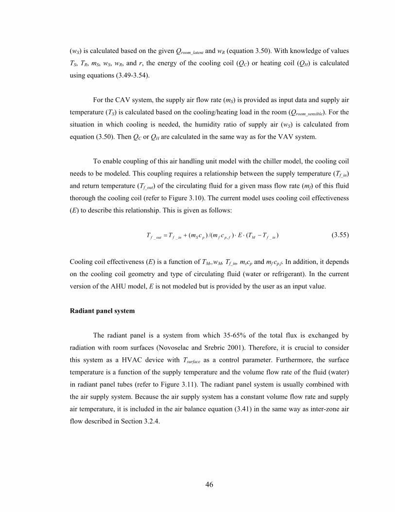
46

(wS) is calculated based on the given Qroom_latent and wR (equation 3.50). With knowledge of values

TS, TR, mS, wS, wR, and r, the energy of the cooling coil (QC) or heating coil (QH) is calculated

using equations (3.49-3.54).

For the CAV system, the supply air flow rate (mS) is provided as input data and supply air

temperature (TS) is calculated based on the cooling/heating load in the room (Qroom_sensible). For the

situation in which cooling is needed, the humidity ratio of supply air (wS) is calculated from

equation (3.50). Then QC or QH are calculated in the same way as for the VAV system.

To enable coupling of this air handling unit model with the chiller model, the cooling coil

needs to be modeled. This coupling requires a relationship between the supply temperature (Tf_in)

and return temperature (Tf_out) of the circulating fluid for a given mass flow rate (mf) of this fluid

thorough the cooling coil (refer to Figure 3.10). The current model uses cooling coil effectiveness

(E) to describe this relationship. This is given as follows:

)()/()( _,__ infMfpfpSinfoutf TTEcmcmTT −⋅⋅+= (3.55)

Cooling coil effectiveness (E) is a function of TM,,wM, Tf_in, mscp and mf cp,f. In addition, it depends

on the cooling coil geometry and type of circulating fluid (water or refrigerant). In the current

version of the AHU model, E is not modeled but is provided by the user as an input value.

Radiant panel system

The radiant panel is a system from which 35-65% of the total flux is exchanged by

radiation with room surfaces (Novoselac and Srebric 2001). Therefore, it is crucial to consider

this system as a HVAC device with Tsurface as a control parameter. Furthermore, the surface

temperature is a function of the supply temperature and the volume flow rate of the fluid (water)

in radiant panel tubes (refer to Figure 3.11). The radiant panel system is usually combined with

the air supply system. Because the air supply system has a constant volume flow rate and supply

air temperature, it is included in the air balance equation (3.41) in the same way as inter-zone air

flow described in Section 3.2.4.

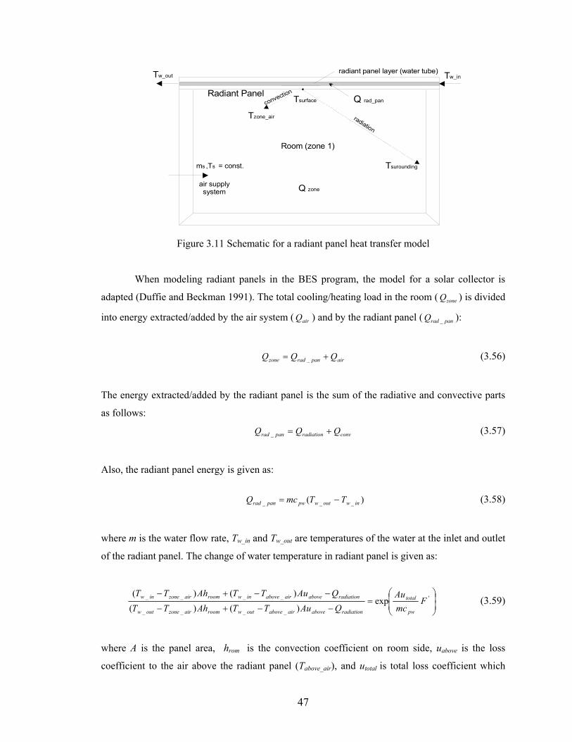
47

Room (zone 1)

Radiant Panelconvection

Tsurface

Tsurounding

Tzone_air radiation

Q rad_pan

radiant panel layer (water tube)

air supplysystem

m ,T = const.s s

Q zone

Tw_out Tw_in

Figure 3.11 Schematic for a radiant panel heat transfer model

When modeling radiant panels in the BES program, the model for a solar collector is

adapted (Duffie and Beckman 1991). The total cooling/heating load in the room ( zoneQ ) is divided

into energy extracted/added by the air system ( airQ ) and by the radiant panel ( panradQ _ ):

airpanradzone QQQ += _ (3.56)

The energy extracted/added by the radiant panel is the sum of the radiative and convective parts

as follows:

convradiationpanrad QQQ +=_ (3.57)

Also, the radiant panel energy is given as:

)( ___ inwoutwpwpanrad TTmcQ −= (3.58)

where m is the water flow rate, Tw_in and Tw_out are temperatures of the water at the inlet and outlet

of the radiant panel. The change of water temperature in radiant panel is given as:

=

−−+−

−−+− '

____

____ exp)()(

)()(F

mcAu

QAuTTAhTTQAuTTAhTT

pw

total

radiationaboveairaboveoutwroomairzoneoutw

radiationaboveairaboveinwroomairzoneinw (3.59)

where A is the panel area, hrom is the convection coefficient on room side, uabove is the loss

coefficient to the air above the radiant panel (Tabove_air), and utotal is total loss coefficient which

48

encompasses the convection on the room side and the loss above the radiant panel. It is calculated

as aboveroomtotal uchu ⋅+= , where c is a correction for unequal Tabove_air and Tzone_air. It can be

approximated as )2/()2( ______ airzoneoutwinwairaboveoutwinw TTTTTTc ⋅−+⋅−+= . The coefficient F ’ is the

efficiency factor of radiant panel (collector) defined by geometry and construction of the radiant

panel (Duffie and Beckman 1991).

The system of equations (3.56-3.59) is a closed system which enables the calculation of

water inlet ( inwT _ ) and outlet temperature ( outwT _ ) using known values of radiationQ and convQ . Heat

fluxes radiationQ and convQ are solved by the energy balance equations of the room together with

room temperature ( airzoneT _ ) and temperature of the air above the panel ( airaboveT _ ). For a given

mass flow rate of water ‘m’, this model provides the relationship between the inlet inwT _ and

outlet outwT _ water temperatures. This enables further coupling of the radiant panel system with

the chiller model.

Pure convective system

The heating load (Qroom) for pure convective devices such as baseboard heaters or fan coil

systems in a heating regime is equal to the load of the heating plant (QH) that is reduced by the

amount of energy lost in the pipe system. This is defined by the heating distribution system

efficiency (ηdistribut_system) as follows:

systemdistributHroom QQ _η⋅= (3.60)

For fan coil systems in cooling regime, condensation may appear on the fan-coil heat exchanger.

This primarily depends on surface temperature of the fan coil heat exchanger (TFC_surface) and

room dew-point temperature (Tdp). In the model implemented in the BES program, it is assumed

that TFC_surface > Tdp. This means that the water supply temperature for the fan coil is controlled in

order to avoid condensation. Therefore, it follows that:

)( __ inwoutwproom TTmcQ −= (3.61)

where m is the water flow rate, Tw_in is the inlet and Tw_out the outlet water temperatures. The

relationship between inlet inwT _ and outlet outwT _ water temperatures enables further coupling of

the fan coil system with the chiller.

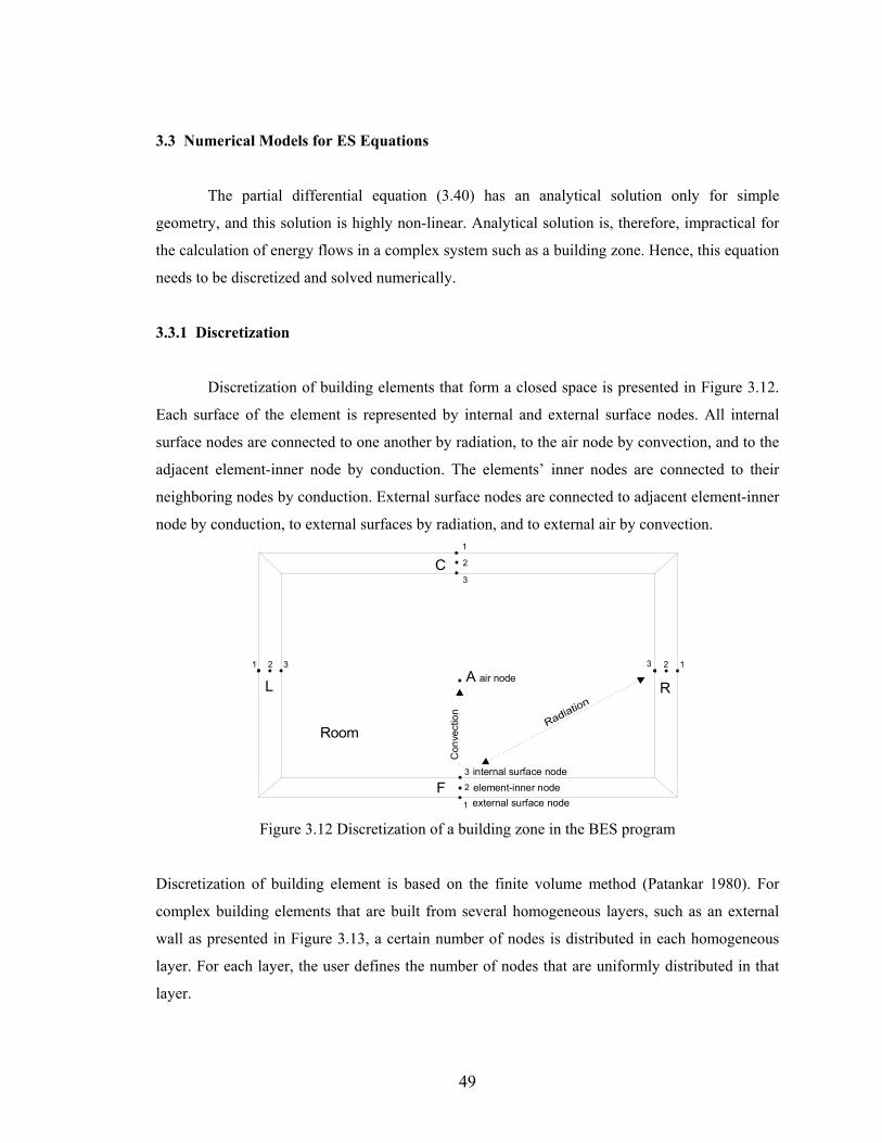
49

3.3 Numerical Models for ES Equations

The partial differential equation (3.40) has an analytical solution only for simple

geometry, and this solution is highly non-linear. Analytical solution is, therefore, impractical for

the calculation of energy flows in a complex system such as a building zone. Hence, this equation

needs to be discretized and solved numerically.

3.3.1 Discretization

Discretization of building elements that form a closed space is presented in Figure 3.12.

Each surface of the element is represented by internal and external surface nodes. All internal

surface nodes are connected to one another by radiation, to the air node by convection, and to the

adjacent element-inner node by conduction. The elements’ inner nodes are connected to their

neighboring nodes by conduction. External surface nodes are connected to adjacent element-inner

node by conduction, to external surfaces by radiation, and to external air by convection.

Room

F

C

L R

1

1

11

2

2

22

3

3

33A air node

internal surface node

external surface nodeelement-inner node

Con

vect

ion

Figure 3.12 Discretization of a building zone in the BES program

Discretization of building element is based on the finite volume method (Patankar 1980). For

complex building elements that are built from several homogeneous layers, such as an external

wall as presented in Figure 3.13, a certain number of nodes is distributed in each homogeneous

layer. For each layer, the user defines the number of nodes that are uniformly distributed in that

layer.

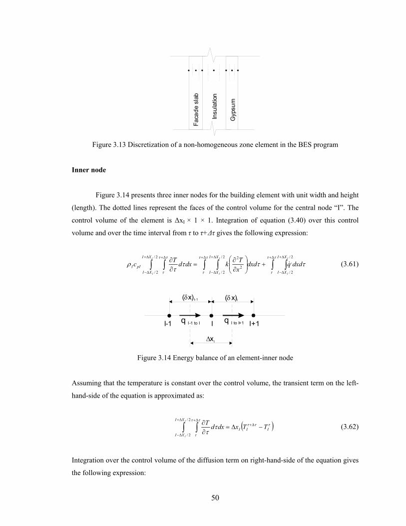
50

Faca

de s

lab

Insu

latio

n

Gyp

sum

Figure 3.13 Discretization of a non-homogeneous zone element in the BES program

Inner node

Figure 3.14 presents three inner nodes for the building element with unit width and height

(length). The dotted lines represent the faces of the control volume for the central node “I”. The

control volume of the element is ∆xI × 1 × 1. Integration of equation (3.40) over this control

volume and over the time interval from τ to τ+∆τ gives the following expression:

∫ ∫∫ ∫ ∫∫∆+ ∆+

∆−

∆+

∆−

∆+ ∆+

∆−

∆+

+

∂∂

=∂∂ ττ

τ

ττ

τ

ττ

τ

ττττ

ρ2/

2/

, 2/

2/

2/

2/2

2 I

I

I

I

I

I

XI

XI

XI

XI

XI

XIpII dxdqdxd

xTkdxdTc & (3.61)

( x)δ I- 1 ( x)Iδ

∆xI

I-1 I I+1q I-1 to I q I to I+1

Figure 3.14 Energy balance of an element-inner node

Assuming that the temperature is constant over the control volume, the transient term on the left-

hand-side of the equation is approximated as:

( )∫ ∫∆+

∆−

∆+∆+

−∆=∂∂2/

2/

I

I

XI

XIIII TTxdxdT τττ

ττ

τ

ττ

(3.62)

Integration over the control volume of the diffusion term on right-hand-side of the equation gives

the following expression:

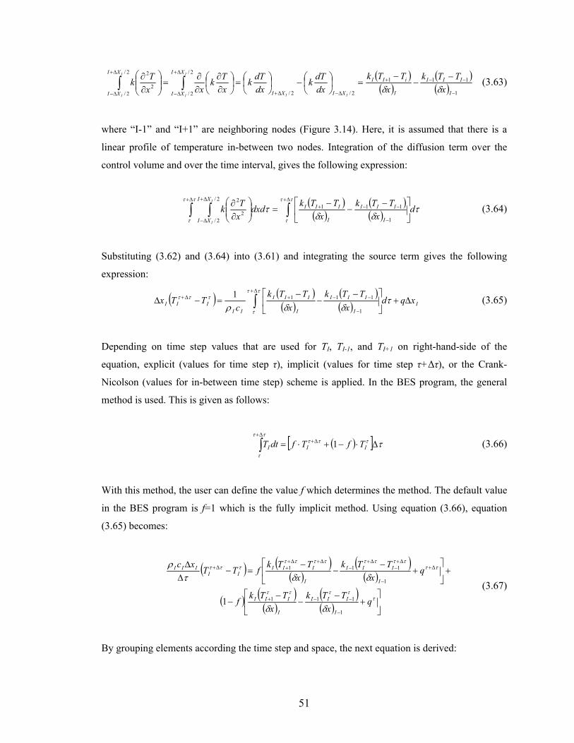
51

( )( )

( )( ) 1

111

2/2/

2/

2/

2/

2/2

2

−

−−+

∆−∆+

∆+

∆−

∆+

∆−

−−

−=

−

=

∂∂

∂∂

=

∂∂

∫∫I

III

I

iII

XIXI

XI

XI

XI

XI xTTk

xTTk

dxdTk

dxdTk

xTk

xxTk

II

I

I

I

Iδδ

(3.63)

where “I-1” and “I+1” are neighboring nodes (Figure 3.14). Here, it is assumed that there is a

linear profile of temperature in-between two nodes. Integration of the diffusion term over the

control volume and over the time interval, gives the following expression:

( )( )

( )( ) τδδ

τττ

τ

ττ

τ

dx

TTkx

TTkdxdxTk

I

III

I

IIIXI

XI

I

I

∫∫ ∫∆+

−

−−+∆+ ∆+

∆−

−−

−=

∂∂

1

1112/

2/2

2

(3.64)

Substituting (3.62) and (3.64) into (3.61) and integrating the source term gives the following

expression:

( ) ( )( )

( )( ) I

I

III

I

III

IIIII xqd

xTTk

xTTk

cTTx ∆+

−−

−=−∆ ∫

∆+

−

−−+∆+ τδδρ

ττ

τ

τττ

1

1111 (3.65)

Depending on time step values that are used for TI, TI-1, and TI+1 on right-hand-side of the

equation, explicit (values for time step τ), implicit (values for time step τ+∆τ), or the Crank-

Nicolson (values for in-between time step) scheme is applied. In the BES program, the general

method is used. This is given as follows:

( )[ ] ττττττ

τ

∆⋅−+⋅= ∆+∆+

∫ III TfTfdtT 1 (3.66)

With this method, the user can define the value f which determines the method. The default value

in the BES program is f=1 which is the fully implicit method. Using equation (3.66), equation

(3.65) becomes:

( ) ( )( )

( )( )

( ) ( )( )

( )( )

+

−−

−−

+

+

−−

−=−

∆∆

−

−−+

∆+

−

∆+−

∆+−

∆+∆++∆+

τττττ

ττττττττττ

τττ

δδ

δδτρ

qx

TTkx

TTkf

qx

TTkx

TTkfTTxc

I

III

I

III

I

III

I

IIIII

III

1

111

1

111

1

(3.67)

By grouping elements according the time step and space, the next equation is derived:

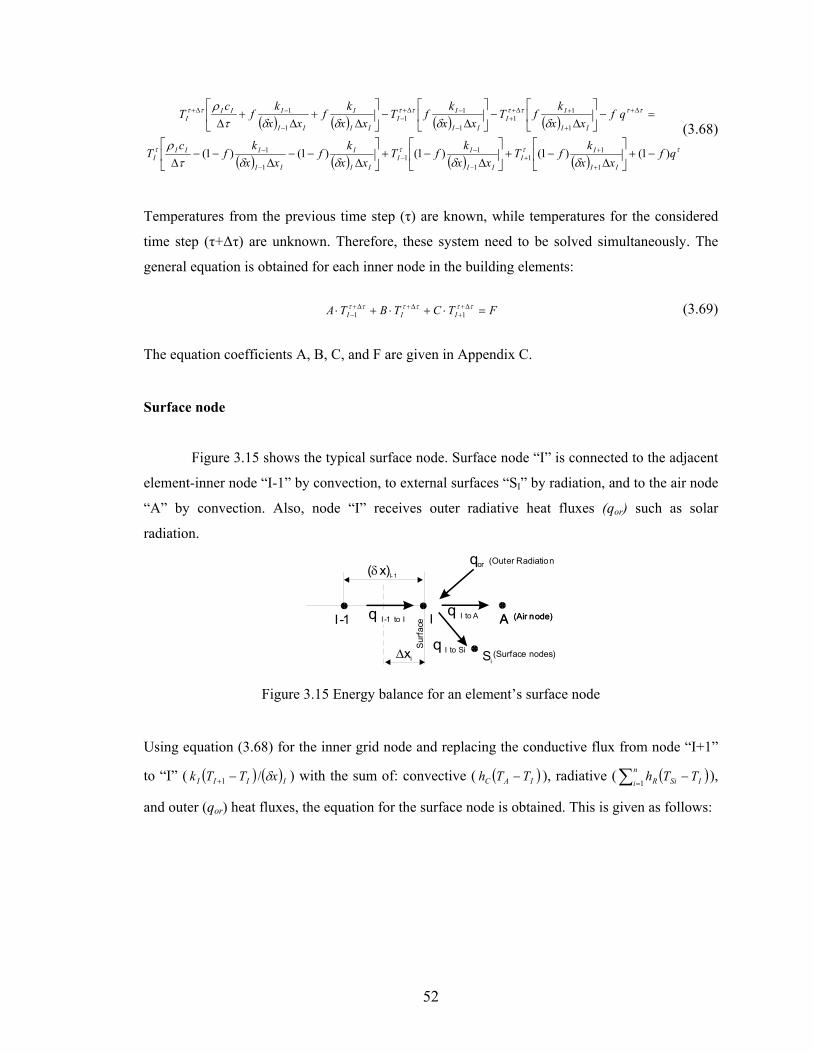
52

( ) ( ) ( ) ( )

( ) ( ) ( ) ( )ττττ

ττττττττ

δδδδτρ

δδδδτρ

qfxx

kfT

xxk

fTxx

kf

xxk

fc

T

qfxx

kfT

xxk

fTxx

kf

xxk

fc

T

II

II

II

II

II

I

II

IIII

II

II

II

II

II

I

II

IIII

)1()1()1()1()1(

1

11

1

11

1

1

1

11

1

11

1

1

−+

∆

−+

∆

−+

∆

−−∆

−−∆

=−

∆

−

∆

−

∆

+∆

+∆

+

++

−

−−

−

−

∆+

+

+∆++

−

−∆+−

−

−∆+

(3.68)

Temperatures from the previous time step (τ) are known, while temperatures for the considered

time step (τ+∆τ) are unknown. Therefore, these system need to be solved simultaneously. The

general equation is obtained for each inner node in the building elements:

FTCTBTA III =⋅+⋅+⋅ ∆+

+∆+∆+

−ττττττ

11 (3.69)

The equation coefficients A, B, C, and F are given in Appendix C.

Surface node

Figure 3.15 shows the typical surface node. Surface node “I” is connected to the adjacent

element-inner node “I-1” by convection, to external surfaces “SI” by radiation, and to the air node

“A” by convection. Also, node “I” receives outer radiative heat fluxes (qor) such as solar

radiation.

( x)δ I- 1

∆xI

I -1 A (Air node)I

Surfa

ce

q I-1 to Iq I to A

qor

A (Air node)

Si(Surface nodes)

q I to Si

(Outer Radiation)

Figure 3.15 Energy balance for an element’s surface node

Using equation (3.68) for the inner grid node and replacing the conductive flux from node “I+1”

to “I” ( ( ) ( )IIII xTTk δ/1 −+ ) with the sum of: convective ( ( )IAC TTh − ), radiative ( ( )∑ =−

n

i ISiR TTh1

),

and outer (qor) heat fluxes, the equation for the surface node is obtained. This is given as follows:

53

( ) ( )

( )

( )τ

τττ

ττ

ττ

τττ

ττττ

ττττττ

ττττ

ττ

δ

δτρ

δδτρ

orI

n

iiSiR

I

CA

II

II

I

n

iiR

I

C

II

IIIIor

I

n

iSiiR

I

CA

II

II

I

n

iiR

I

C

II

IIII

qfx

Thf

xhfT

xxkfT

x

hf

xhf

xxkfcTqf

x

Thf

xhfT

xxkfT

x

hf

xhf

xxkfcT

)1()1( )1()1(

)1()1()1(

1,,

1

11

1,

1

11,

1

11

1,

1

1

−+∆

⋅−+

∆

−+

∆

−

+

∆−−

∆−−

∆−−

∆=−

∆

⋅

−

∆

−

∆

−

∆+

∆+

∆+

∆

∑

∑∑

∑

=

−

−−

=

−

−∆+=

∆+∆+

∆+∆+

−

−∆+−

=

∆+∆+

−

−∆+

(3.70)

This equation can be written in a general form for each internal surface node as:

FTSTRTBTAn

iiSAII =⋅+⋅+⋅+⋅ ∑

=

∆+∆+∆+∆+−

1,1

ττττττττ (3.71)

For external surface nodes, the general equation is written in a different form because

these surfaces exchange the energy with elements that have known temperatures (or the

temperatures are calculated based on input data for a considered time step). These elements are

external air, sky, and ground, or soil for surfaces in contact with the ground. Because the

temperatures of these elementals are independent of surface temperature (TI), they are moved to

the right-hand-side of the equation to be a part of the free coefficient (F). The general form of

equation for external surface is given as:

FTCTB II =⋅+⋅ ∆++

∆+ ττττ1 (3.72)

Coefficients A, B, C, R, S, and F for internal and external surface nodes are given in Appendix C.

Air node

Room air in the BES program is represented with a single node (refer to Figure 3.12).

This air node is connected to each surface node by convection, to external air by the mass flow

rate of infiltration air, and to the HVAC supply system by mass flow rate of supply air. Also, air

node “A” receives energy from other internal heat sources (Qis), which includes the convective

source from occupants, for instance.

54

Integrating the energy conservation equation for air (3.41) over the room volume (Vroom)

and over the time interval ∆τ, the following equation is obtained:

room

is

room

m

jjEjp

room

n

iiSiC

room

m

jjp

room

n

iiC

IpIA

room

is

room

m

jjEjp

room

n

iiSiC

room

m

jjp

room

n

iiC

IpIA

VQ

fV

Tmcf

V

TAhf

V

mcf

V

Ahf

cT

VQ

fV

Tmcf

V

TAhf

V

mcf

V

Ahf

cT

τττττ

ττ

τττ

ττττ

ττττττττ

ττ

τρ

τρ

)1()(

)1()(

)1(

)1()(

)1()(

)()(

1,,

1,

1,

1,1,,

1,

1,

1,

−+

⋅

−+⋅

−

+

−−−−∆

=−

⋅

−⋅

−

++∆

∑∑

∑∑∑

∑∑∑

==

==∆+

=

∆+∆+

=

∆+∆+

=

∆+

=

∆+

∆+

(3.73)

The general form of air node equation is given as:

FTITETD

m

jj,E

n

ii,SA =⋅+⋅+⋅ ∑∑

=

∆+

=

∆+∆+

11

ττττττ (3.74)

where coefficients D, E, I, and F are given in Appendix C.

3.3.2 System of Equations

The energy conservation equations for each element-inner (equations 3.68) and surface

nodes (equations 3.70) together with the air node (equation 3.73) form a system of linear

equations. In the case of a fully implicit scheme, this system solves temperatures of all building

elements for a time step (τ+∆τ) based on boundary conditions for that time step, and temperatures

of all building elements for the previous time step (τ). In the case of the Crank-Nicolson scheme

(f=0.5), boundary conditions from the previous time step are also used. With the explicit scheme,

solving the simultaneous equations is unnecessary because the temperature distribution for the

considered time step (τ+∆τ) is explicitly obtainable from the temperatures of previous time step.

In the BES program, an explicit scheme is possible but completely impractical because of the

numerical stability problem. To obtain a numerically stable system with an explicit scheme

(Patankar 1980), a selected time step (∆τ) should satisfy:

)2/()( 2 kxcp ∆<∆ ρτ (3.75)

55

for each node of the building zone. This means that for conductivity (k), density (ρ) and specific

capacity (cp) of building materials and typical discretization, where ∆x is in range of 0.001 to 0.1

m, the selected time step (∆τ) should be less than a second. Therefore, in the BES program the

system of equations is solved simultaneously (using implicit schemes).

Energy flow by heat transfer mechanisms such as radiation, convection, and inter-zone

air flow are described by non-linear equations. Linearization of these phenomena is described in

Section 3.2.2. In the solution procedure, radiative heat exchange coefficients (hr) are calculated

using the temperature distribution from the previous time step. Surface convection coefficient (h)

or inter-zone air mass flow (mi) are obtained in the same manner. Because these coefficients are

based on temperature values from the previous time step, it is very important to have a realistic

initial temperature distribution. This problem is solved by using a “warming” calculation

procedure which defines the initial temperatures. This “warming” procedure is described in detail

in Chapter 6.

The equation’s right-hand-side coefficient (F) is updated for each time step based on the

calculated temperature distribution in the previous time step. Also, for surface nodes, this term

defines the “outer” radiative heat flux (qor) which is completely independent of the surface

temperature. For internal surfaces, the outer radiative heat flux contains absorbed direct and

diffuse solar radiation, lighting short wave radiation, and radiation from internal sources. For

external surfaces, “outer” radiative heat flux contains absorbed diffuse and direct solar radiation.

For the air node, coefficient (F) contains a term which defines internal convective heat flux (Qis)

which is also independent of temperature distribution. These heat fluxes are also updated for each

calculation step based on input data such as weather condition or the power and the working

period of a lighting system.

For all surface nodes, the coefficients A, R, and S in equation (3.71) and C in equation

(3.72) are updated for each time step because of the change of the radiative heat exchange

coefficients (hr) and surface convection coefficient (h) at internal and external surfaces. For the

same reason, all air node coefficients (D, E, I, and F) are updated in each time step. Only for

internal nodes (equation 3.69), coefficients A, B, and C do not change during the calculation

procedure because temperature independent conduction coefficients (k) are assumed.

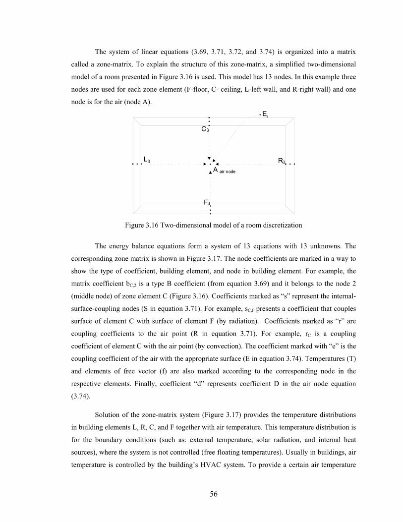
56

The system of linear equations (3.69, 3.71, 3.72, and 3.74) is organized into a matrix

called a zone-matrix. To explain the structure of this zone-matrix, a simplified two-dimensional

model of a room presented in Figure 3.16 is used. This model has 13 nodes. In this example three

nodes are used for each zone element (F-floor, C- ceiling, L-left wall, and R-right wall) and one

node is for the air (node A).

F

C

L R

3

3

33

A air node

Ei

Figure 3.16 Two-dimensional model of a room discretization

The energy balance equations form a system of 13 equations with 13 unknowns. The

corresponding zone matrix is shown in Figure 3.17. The node coefficients are marked in a way to

show the type of coefficient, building element, and node in building element. For example, the

matrix coefficient bC,2 is a type B coefficient (from equation 3.69) and it belongs to the node 2

(middle node) of zone element C (Figure 3.16). Coefficients marked as “s” represent the internal-

surface-coupling nodes (S in equation 3.71). For example, sC,F presents a coefficient that couples

surface of element C with surface of element F (by radiation). Coefficients marked as “r” are

coupling coefficients to the air point (R in equation 3.71). For example, rC is a coupling

coefficient of element C with the air point (by convection). The coefficient marked with “e” is the

coupling coefficient of the air with the appropriate surface (E in equation 3.74). Temperatures (T)

and elements of free vector (f) are also marked according to the corresponding node in the

respective elements. Finally, coefficient “d” represents coefficient D in the air node equation

(3.74). Solution of the zone-matrix system (Figure 3.17) provides the temperature distributions

in building elements L, R, C, and F together with air temperature. This temperature distribution is

for the boundary conditions (such as: external temperature, solar radiation, and internal heat

sources), where the system is not controlled (free floating temperatures). Usually in buildings, air

temperature is controlled by the building’s HVAC system. To provide a certain air temperature

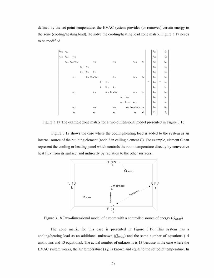
57

defined by the set point temperature, the HVAC system provides (or removes) certain energy to

the zone (cooling/heating load). To solve the cooling/heating load zone matrix, Figure 3.17 needs

to be modified.

bC,1 cC,1 TC1 fC1

aC,2 bC,2 cC,2 TC2 fC2

aC,3 bC,3+sC,C sC,F sC,L sC,R rC TC3 fC3

bF,1 cF,1 TF1 fF1

aF,2 bF,2 cF,2 TF2 fF2

sF,C aF,3 bF,3+sF,F sF,L aF,R rF TF3 fF3

bL,1 cL,1 × TL1 = fL1

aL,2 bL,2 cL,2 TL2 fL2

sL,C sL,F aL,3 bL,3+sL,L sL,R rL TL3 fL3

bR,1 cR,1 TR1 fR1

aR,2 bR,12 cR, 2 TR2 fR2

sR,C sR,F sR,L aR,3 bR,13+sR,R rR TR3 fR3

eC eF eL eR d TA fA

Figure 3.17 The example zone matrix for a two-dimensional model presented in Figure 3.16

Figure 3.18 shows the case where the cooling/heating load is added to the system as an

internal source of the building element (node 2 in ceiling element C). For example, element C can

represent the cooling or heating panel which controls the room temperature directly by convective

heat flux from its surface, and indirectly by radiation to the other surfaces.

Room

F

C

L R

1

1

11

2

2

22

3

3

33

A air node

Con

vect

ion

Q HVAC

Figure 3.18 Two-dimensional model of a room with a controlled source of energy (QHVAC)

The zone matrix for this case is presented in Figure 3.19. This system has a

cooling/heating load as an additional unknown (QHVAC) and the same number of equations (14

unknowns and 13 equations). The actual number of unknowns is 13 because in the case where the

HVAC system works, the air temperature (TA) is known and equal to the set point temperature. In

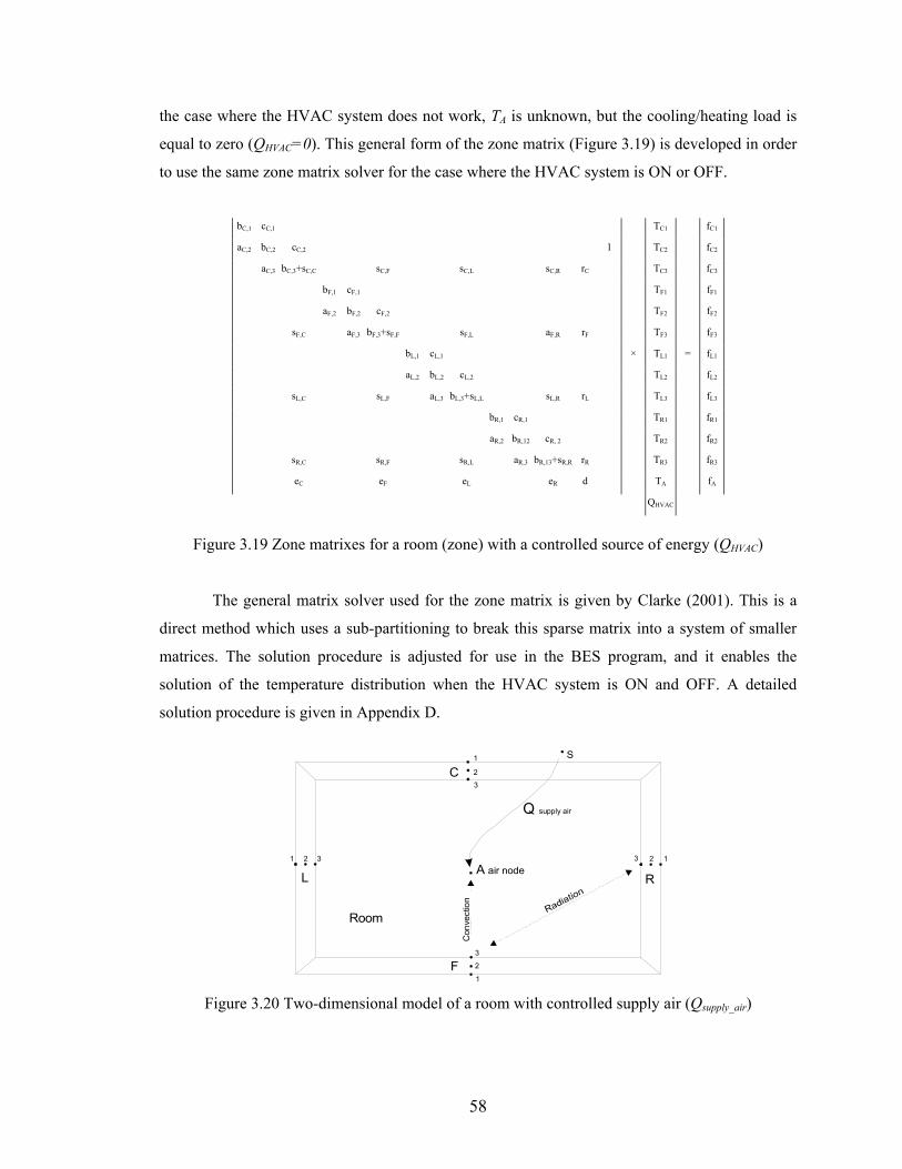
58

the case where the HVAC system does not work, TA is unknown, but the cooling/heating load is

equal to zero (QHVAC=0). This general form of the zone matrix (Figure 3.19) is developed in order

to use the same zone matrix solver for the case where the HVAC system is ON or OFF.

bC,1 cC,1 TC1 fC1

aC,2 bC,2 cC,2 1 TC2 fC2

aC,3 bC,3+sC,C sC,F sC,L sC,R rC TC3 fC3

bF,1 cF,1 TF1 fF1

aF,2 bF,2 cF,2 TF2 fF2

sF,C aF,3 bF,3+sF,F sF,L aF,R rF TF3 fF3

bL,1 cL,1 × TL1 = fL1

aL,2 bL,2 cL,2 TL2 fL2

sL,C sL,F aL,3 bL,3+sL,L sL,R rL TL3 fL3

bR,1 cR,1 TR1 fR1

aR,2 bR,12 cR, 2 TR2 fR2

sR,C sR,F sR,L aR,3 bR,13+sR,R rR TR3 fR3

eC eF eL eR d TA fA

QHVAC

Figure 3.19 Zone matrixes for a room (zone) with a controlled source of energy (QHVAC)

The general matrix solver used for the zone matrix is given by Clarke (2001). This is a

direct method which uses a sub-partitioning to break this sparse matrix into a system of smaller

matrices. The solution procedure is adjusted for use in the BES program, and it enables the

solution of the temperature distribution when the HVAC system is ON and OFF. A detailed

solution procedure is given in Appendix D.

Room

F

C

L R

1

1

11

2

2

22

3

3

33

A air node

Con

vect

ion

Q supply air

S

Figure 3.20 Two-dimensional model of a room with controlled supply air (Qsupply_air)

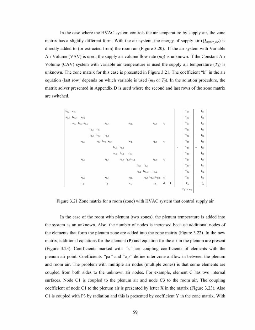
59

In the case where the HVAC system controls the air temperature by supply air, the zone

matrix has a slightly different form. With the air system, the energy of supply air (Qsupply_aur) is

directly added to (or extracted from) the room air (Figure 3.20). If the air system with Variable

Air Volume (VAV) is used, the supply air volume flow rate (mS) is unknown. If the Constant Air

Volume (CAV) system with variable air temperature is used the supply air temperature (TS) is

unknown. The zone matrix for this case is presented in Figure 3.21. The coefficient “k” in the air

equation (last row) depends on which variable is used (mS or TS). In the solution procedure, the

matrix solver presented in Appendix D is used where the second and last rows of the zone matrix

are switched.

bC,1 cC,1 TC1 fC1

aC,2 bC,2 cC,2 TC2 fC2

aC,3 bC,3+sC,C sC,F sC,L sC,R rC TC3 fC3

bF,1 cF,1 TF1 fF1

aF,2 bF,2 cF,2 TF2 fF2

sF,C aF,3 bF,3+sF,F sF,L aF,R rF TF3 fF3

bL,1 cL,1 × TL1 = fL1

aL,2 bL,2 cL,2 TL2 fL2

sL,C sL,F aL,3 bL,3+sL,L sL,R rL TL3 fL3

bR,1 cR,1 TR1 fR1

aR,2 bR,12 cR, 2 TR2 fR2

sR,C sR,F sR,L aR,3 bR,13+sR,R rR TR3 fR3

eC eF eL eR d k TA fA

TS or mS

Figure 3.21 Zone matrix for a room (zone) with HVAC system that control supply air

In the case of the room with plenum (two zones), the plenum temperature is added into

the system as an unknown. Also, the number of nodes is increased because additional nodes of

the elements that form the plenum zone are added into the zone matrix (Figure 3.22). In the new

matrix, additional equations for the element (P) and equation for the air in the plenum are present

(Figure 3.23). Coefficients marked with “k” are coupling coefficients of elements with the

plenum air point. Coefficients “pa” and “ap” define inter-zone airflow in-between the plenum

and room air. The problem with multiple air nodes (multiple zones) is that some elements are

coupled from both sides to the unknown air nodes. For example, element C has two internal

surfaces. Node C1 is coupled to the plenum air and node C3 to the room air. The coupling

coefficient of node C1 to the plenum air is presented by letter X in the matrix (Figure 3.23). Also

C1 is coupled with P3 by radiation and this is presented by coefficient Y in the zone matrix. With

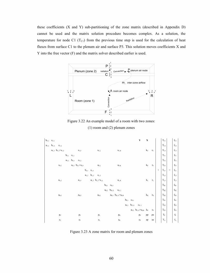
60

these coefficients (X and Y) sub-partitioning of the zone matrix (described in Appendix D)

cannot be used and the matrix solution procedure becomes complex. As a solution, the

temperature for node C1 (TC1) from the previous time step is used for the calculation of heat

fluxes from surface C1 to the plenum air and surface P3. This solution moves coefficients X and

Y into the free vector (F) and the matrix solver described earlier is used.

Room (zone 1)

Plenum (zone 2)

F

C

L R

1

1

11

2

2

22

3

3

33 A

radiation Convection

Radiation

P plenum air node

1

2

3

Con

vect

ion

P

room air node

inter-zone airflowmA P

Figure 3.22 An example model of a room with two zones:

(1) room and (2) plenum zones

bC,1 cC,1 Y X TC1 fC1

aC,2 bC,2 cC,2 TC2 fC2

aC,3 bC,3+sC,C sC,F sC,L sC,R kC rC TC3 fC3

bF,1 cF,1 TF1 fF1

aF,2 bF,2 cF,2 TF2 fF2

sF,C aF,3 bF,3+sF,F aF,L aF,R kF rF TF3 fF3

bL,1 cL,1 × TL1 = fL1

aL,2 bL,2 cL,2 TL2 fL2

aL,C aL,F aL,3 bL,3+sL,L aL,R kL rL TL3 fL3

bR,1 cR,1 TR1 fR1

aR,2 bR,12 cR, 2 TR2 fR2

aR,C aR,F aR,L aR,3 bR,13+sR,R kR rR TR3 fR3

bP,1 cP,1 TP1 fP1

aP,2 bP,12 cP, 2 TP2 fP2

aP,3 bP,13+sR,R kP rP TP3 fP3

pC pF pL pR pP pp pa TP fP

eC eF eL eR eP ap aa TA fA

Figure 3.23 A zone matrix for room and plenum zones

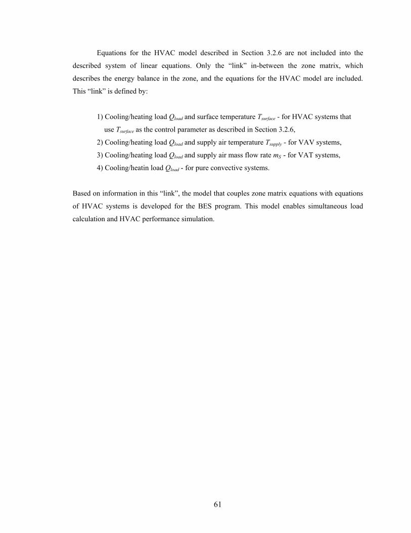
61

Equations for the HVAC model described in Section 3.2.6 are not included into the

described system of linear equations. Only the “link” in-between the zone matrix, which

describes the energy balance in the zone, and the equations for the HVAC model are included.

This “link” is defined by:

1) Cooling/heating load Qload and surface temperature Tsurface - for HVAC systems that

use Tsurface as the control parameter as described in Section 3.2.6,

2) Cooling/heating load Qload and supply air temperature Tsupply - for VAV systems,

3) Cooling/heating load Qload and supply air mass flow rate mS - for VAT systems,

4) Cooling/heatin load Qload - for pure convective systems.

Based on information in this “link”, the model that couples zone matrix equations with equations

of HVAC systems is developed for the BES program. This model enables simultaneous load

calculation and HVAC performance simulation.

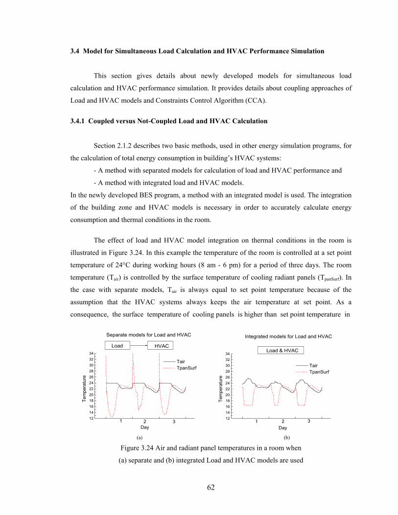
62

3.4 Model for Simultaneous Load Calculation and HVAC Performance Simulation

This section gives details about newly developed models for simultaneous load

calculation and HVAC performance simulation. It provides details about coupling approaches of

Load and HVAC models and Constraints Control Algorithm (CCA).

3.4.1 Coupled versus Not-Coupled Load and HVAC Calculation

Section 2.1.2 describes two basic methods, used in other energy simulation programs, for

the calculation of total energy consumption in building’s HVAC systems:

- A method with separated models for calculation of load and HVAC performance and

- A method with integrated load and HVAC models.

In the newly developed BES program, a method with an integrated model is used. The integration

of the building zone and HVAC models is necessary in order to accurately calculate energy

consumption and thermal conditions in the room.

The effect of load and HVAC model integration on thermal conditions in the room is

illustrated in Figure 3.24. In this example the temperature of the room is controlled at a set point

temperature of 24°C during working hours (8 am - 6 pm) for a period of three days. The room

temperature (Tair) is controlled by the surface temperature of cooling radiant panels (TpanSurf). In

the case with separate models, Tair is always equal to set point temperature because of the

assumption that the HVAC systems always keeps the air temperature at set point. As a

consequence, the surface temperature of cooling panels is higher than set point temperature in

0 240 480 720121416182022242628303234

Separate models for Load and HVAC

HVAC

2 31

Tair TpanSurf

Tem

pera

ture

Day

Load

0 240 480 720

121416182022242628303234

Integrated models for Load and HVAC

enter text here

21 3

Tair TpanSurf

Tem

pera

ture

Day

Load & HVAC

(a) (b)

Figure 3.24 Air and radiant panel temperatures in a room when

(a) separate and (b) integrated Load and HVAC models are used

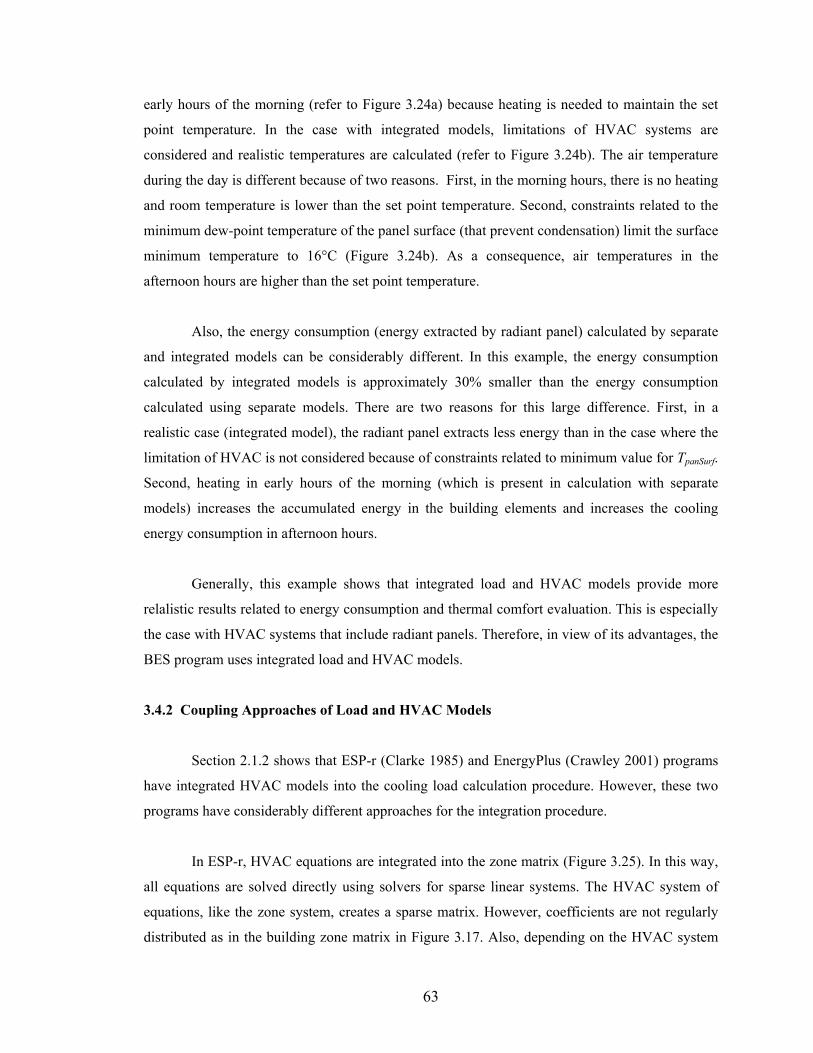
63

early hours of the morning (refer to Figure 3.24a) because heating is needed to maintain the set

point temperature. In the case with integrated models, limitations of HVAC systems are

considered and realistic temperatures are calculated (refer to Figure 3.24b). The air temperature

during the day is different because of two reasons. First, in the morning hours, there is no heating

and room temperature is lower than the set point temperature. Second, constraints related to the

minimum dew-point temperature of the panel surface (that prevent condensation) limit the surface

minimum temperature to 16°C (Figure 3.24b). As a consequence, air temperatures in the

afternoon hours are higher than the set point temperature.

Also, the energy consumption (energy extracted by radiant panel) calculated by separate

and integrated models can be considerably different. In this example, the energy consumption

calculated by integrated models is approximately 30% smaller than the energy consumption

calculated using separate models. There are two reasons for this large difference. First, in a

realistic case (integrated model), the radiant panel extracts less energy than in the case where the

limitation of HVAC is not considered because of constraints related to minimum value for TpanSurf.

Second, heating in early hours of the morning (which is present in calculation with separate

models) increases the accumulated energy in the building elements and increases the cooling

energy consumption in afternoon hours.

Generally, this example shows that integrated load and HVAC models provide more

relalistic results related to energy consumption and thermal comfort evaluation. This is especially

the case with HVAC systems that include radiant panels. Therefore, in view of its advantages, the

BES program uses integrated load and HVAC models.

3.4.2 Coupling Approaches of Load and HVAC Models

Section 2.1.2 shows that ESP-r (Clarke 1985) and EnergyPlus (Crawley 2001) programs

have integrated HVAC models into the cooling load calculation procedure. However, these two

programs have considerably different approaches for the integration procedure.

In ESP-r, HVAC equations are integrated into the zone matrix (Figure 3.25). In this way,

all equations are solved directly using solvers for sparse linear systems. The HVAC system of

equations, like the zone system, creates a sparse matrix. However, coefficients are not regularly

distributed as in the building zone matrix in Figure 3.17. Also, depending on the HVAC system

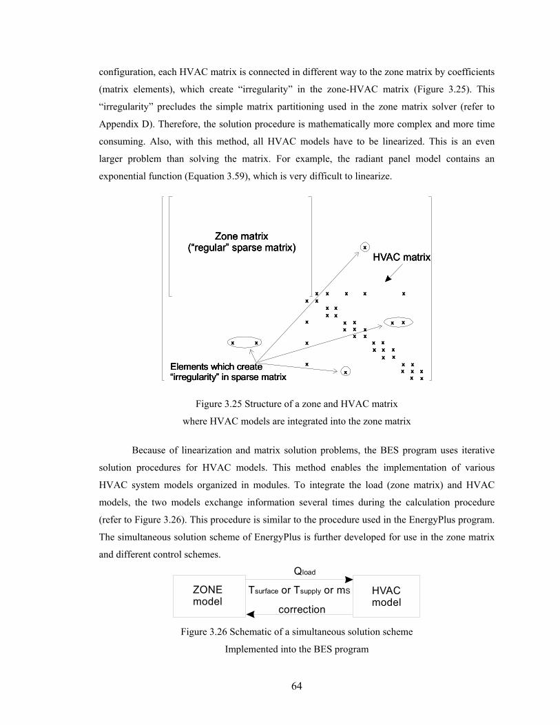
64

configuration, each HVAC matrix is connected in different way to the zone matrix by coefficients

(matrix elements), which create “irregularity” in the zone-HVAC matrix (Figure 3.25). This

“irregularity” precludes the simple matrix partitioning used in the zone matrix solver (refer to

Appendix D). Therefore, the solution procedure is mathematically more complex and more time

consuming. Also, with this method, all HVAC models have to be linearized. This is an even

larger problem than solving the matrix. For example, the radiant panel model contains an

exponential function (Equation 3.59), which is very difficult to linearize.

xx

xx

xx

xx

xx

x

x

xx

x x x xxx

xx

x

xx

xx

xx

x

xxx

x

x

x

x x

x

x

x

x

Elements which create “irregularity” in sparse matrix

HVAC matrix

Zone matrix (“regular” sparse matrix)

xx

xx

xx

xx

xx

x

x

xx

x x x xxx

xx

x

xx

xx

xx

x

xxx

x

x

x

x x

x

x

x

x

Elements which create “irregularity” in sparse matrix

HVAC matrix

Zone matrix (“regular” sparse matrix)

xx

xx

xx

xx

xx

x

x

xx

x x x xxx

xx

x

xx

xx

xx

x

xxx

x

x

x

x x

x

x

x

x

Elements which create “irregularity” in sparse matrix

HVAC matrix

Zone matrix (“regular” sparse matrix)

Figure 3.25 Structure of a zone and HVAC matrix

where HVAC models are integrated into the zone matrix

Because of linearization and matrix solution problems, the BES program uses iterative

solution procedures for HVAC models. This method enables the implementation of various

HVAC system models organized in modules. To integrate the load (zone matrix) and HVAC

models, the two models exchange information several times during the calculation procedure

(refer to Figure 3.26). This procedure is similar to the procedure used in the EnergyPlus program.

The simultaneous solution scheme of EnergyPlus is further developed for use in the zone matrix

and different control schemes.

ZONEmodel

HVACmodel

Tsurface or T or msupply S

Qload

correction Figure 3.26 Schematic of a simultaneous solution scheme

Implemented into the BES program

65

The EnergyPlus program uses the “predictor-corrector” method for integrating the HVAC

system and heating/cooling load models (EnergyPlus 2001). This method is used for the

correction of zone air temperatures in cases where the central plant cannot satisfy heating/cooling

load requirements (Figure 3.26). However, the predictor-corrector scheme used in the EnergyPlus

program corrects only air temperature. The enclosure temperatures and temperatures in building

elements that define thermal energy stored in building are not corrected because the EnergyPlus

program uses conduction transfer functions (EnergyPlus 2001). With the simultaneous solution

scheme developed for the BES program, the relevant correction is returned to the zone matrix

which enables the correction of temperatures in the whole energy simulation domain.

The simultaneous solution scheme used in the BES program consists of the following steps:

(1) For air temperature set point (TAIR): thermal device surface temperature (THVAC) and

required heating/cooling load (QHVAC) are calculated.

(2) Based on these two parameters and outdoor weather data, HVAC models determine if

a thermal plant has the required capacity.

(3) If a thermal plant capacity is not sufficient, the actual capacity (QHVAC) is returned to

the zone matrix (refer to Figure 3.26). After reorganizing the zone matrix, a completely

new temperature distribution in all building elements is calculated.

This simultaneous solution scheme checks only if the power plant has enough

cooling/heating capacity (QHVAC). However, there is a limitation of the HVAC system related to

thermal comfort, air quality, and designed capacity constraints. These constraints are related to

control parameters (Tsupply, Tsurface, and msupply) which are described in Section 3.2.6. For example,

VAV’s power plant has enough cooling capacity but its maximum flow rate (msupply max) is smaller

than the one needed to provide the set point temperature in the room. Otherwise, thermal comfort

may limit the minimum supply temperature with a displacements diffuser. As part of the solution

scheme, the Constraints Control Algorithm was developed and implemented into the BES

program.

3.4.3 Constraints Control Algorithm

The Constraints Control Algorithm is a solution procedure whereby the zone matrix

solver and HVAC modules (HVAC equations solver) exchange information several times for a

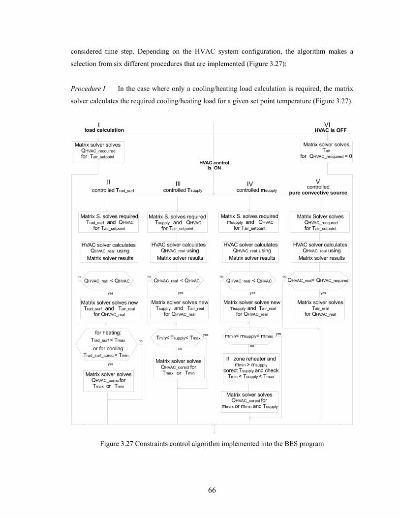
66

considered time step. Depending on the HVAC system configuration, the algorithm makes a

selection from six different procedures that are implemented (Figure 3.27):

Procedure I In the case where only a cooling/heating load calculation is required, the matrix

solver calculates the required cooling/heating load for a given set point temperature (Figure 3.27).

HVAC solver calculates Q using

HVAC_real Matrix solver results

Matrix solver solves newT and T

for Qrad_surf air_real

HVAC_real

T < Trad_surf max

Matrix solver solves Q for T or T

HVAC_corecmax min

for heating:

or for cooling:T > Trad_surf_corec min

yes

yes

no

no

controlled Trad_surf controlled Tsupply

Matrix S.

for

air_setpoint

solves required T and Q

Trad_surf HVAC

HVAC solver calculates Q using

HVAC_real

Matrix solver results

Matrix solver solves new T and T

for Q supply air_real

HVAC_real

T < T < Tmin supply max

Matrix solver solves Q for T or T

HVAC_corect max min

yes

yes

no

no

controlled msupply

Matrix S.

for

air_setpoint

solves required T and Q

Tsupply HVAC

Q < QHVAC_real HVAC Q < QHVAC_real HVAC

HVAC solver calculates Q using

HVAC_real

Matrix solver results

Matrix solver solves new m and T

for Qsupply air_real

HVAC_real

Matrix solver solves Q for

m or m and THVAC_corect

max min supply

yes

yes

no

no

Matrix S.

for

air_setpoint

solves required m and Q

Tsupply HVAC

Q < QHVAC_real HVAC

Matrix Solver

for

air_setpoint

solves Q

THVAC_recqured

Matrix solver

for Q

solves T

= 0air

HVAC_recquired

Matrix solver

for air_setpoint

solves QHVAC_recquired

T

HVAC solver calculates Q using

HVAC_real

Matrix solver results

Matrix solver solves T

for Qair_real HVAC_real

yes

no Q < QHVAC_real HVAC_required

controlled pure convective source

m < m < mmin supply max

If

corect

zone reheater and m > m

T and checkT < T < T

min supplysupply

min supply max

load calculation HVAC is OFF

HVAC control is ON

II III IV V

VII

Figure 3.27 Constraints control algorithm implemented into the BES program

67

Procedure II With the HVAC system where a control parameter is Tsurface, the matrix solver

calculates the cooling/heating load (QHVAC), required Tsurface to keep set point temperature, and all

other temperatures of building elements. Then the program delivers QHVAC to the HVAC module

which checks if the cooling/heating plant has enough capacity to satisfy cooling/heating load.

This check is based on output data from the matrix solver such as Tsurface, convective and radiative

heat flux on the controlled surface. If the cooling/heating plant does not have enough capacity,

the matrix solver solves the new temperature distribution in building elements for a given

cooling/heating capacity. Then, the program performs an additional “check” related to the

limitations of Tsurface. If Tsurface is not within the limit, the matrix solver performs another

computation in order to calculate QHVAC for a new Tsurface.

Procedure III In the case with HVAC system, where a control parameter is Tsupply, the algorithm

is similar to Tsurface. The only difference lies in constraint conditions for Tsupply.

Procedure IV In the case with HVAC system, where a control agent is msupply, the algorithm is

more complex because this HVAC system is a typical VAV system which may or may not have

zone reheaters depending on its configuration. The program first checks if the mass flow rate is

within the relevant range. If the mass flow rate is below the minimum required and zone reheaters

are used, the program corrects the temperature accordingly. Also, a “check” for new temperatures

is performed (refer to Figure 3.27).

Procedure V In case with pure convective HVAC systems, the HVAC module checks if

cooling/heating plant has enough capacity to satisfy cooling/heating load.

Procedure VI In the case where the HVAC system is turned off, the program calculates the air

temperature and all other temperatures for building elements when QHVAC=0.

68

3.5 Validation

Validation of BES was performed in two stages:

1. Validation of program components during code development, and

2. Validation of BES after all program components (models) had been implemented.

3.5.1 Validation of Program Components

During the program code development phase, different models, organized in program

modules, were validated by comparing results obtained with these models with existing and well-

established results. For example, temperature distributions for steady-state and unsteady-state

heat transfer in building elements were first calculated by numerical models implemented in the

BES program. These were then compared to the respective temperature distributions obtained by

existing analytical models. In the same manner, solar angles were calculated by models

implemented in the BES program and compared to solutions provided in ASHRAE Fundamentals

(2001). Also, the view-factor program module was tested using view factor properties (Equation

3.24), symmetrical geometry, and manually calculated solutions.

This section only presents some of the validation tests performed for components of the

BES program. Exact view factors for geometry of the test-building, obtained by the view-factor

program module, are presented in Appendix E. This appendix also contains solar fractions for

transmitted direct and diffuse solar radiation distributions on internal surfaces, which were

calculated by models presented in Section 3.2.2. The presented results (Tables E1-E4)

demonstrate energy conservation, since equations (3.24) and (3.38) are satisfied.

Figure 3.28 shows a comparison between numerical and analytical solutions for unsteady

heat conduction (Equation 3.40). At a certain time step, when the temperature of the wall is

uniform (To), the surface temperature at both sides is decreased (TS). Change of dimensionless

temperature (T-TS/To-TS) during the time at center of the homogeneous wall is plotted for the

exact (analytical) solution and compared with results obtained by the numerical model

implemented into the BES program. Numerical results for different time and space discretization

show the sensitivity of the applied numerical model to this discretization. In the case where the

change in air temperature causes a change of the surface temperature and where the surface heat

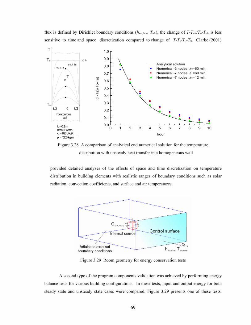
69

flux is defined by Dirichlet boundary conditions (hsurface, Tair), the change of T-Tair/To-Tair is less

sensitive to time and space discretization compared to change of T-TS/To-TS. Clarke (2001)

Ts0

T

-L/2 L/2

τ=0.5 hτ=0 h

τ=1.5 h

To

T

homogenous wall

L = 0.2 mk = 0.5 W/mKc = 920 J/kgK

= 1200 kg/mp

ρ 2

0 1 2 3 4 5 6 7 8 9 100.0

0.1

0.2

0.3

0.4

0.5

0.6

0.7

0.8

0.9

1.0

Analytical solution Numerical -3 nodes, ∆τ=60 min Numerical -7 nodes, ∆τ=60 min Numerical -7 nodes, ∆τ=12 min

(T-T

s)/(T

o-Ts

)

hour

Figure 3.28 A comparison of analytical end numerical solution for the temperature

distribution with unsteady heat transfer in a homogeneous wall

provided detailed analyses of the effects of space and time discretization on temperature

distribution in building elements with realistic ranges of boundary conditions such as solar

radiation, convection coefficients, and surface and air temperatures.

Figure 3.29 Room geometry for energy conservation tests

A second type of the program components validation was achieved by performing energy

balance tests for various building configurations. In these tests, input and output energy for both

steady state and unsteady state cases were compared. Figure 3.29 presents one of these tests.

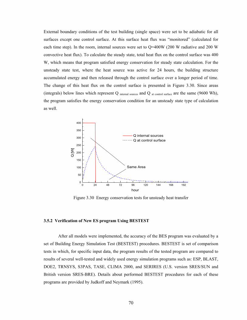
70

External boundary conditions of the test building (single space) were set to be adiabatic for all

surfaces except one control surface. At this surface heat flux was “monitored” (calculated for

each time step). In the room, internal sources were set to Q=400W (200 W radiative and 200 W

convective heat flux). To calculate the steady state, total heat flux on the control surface was 400

W, which means that program satisfied energy conservation for steady state calculation. For the

unsteady state test, where the heat source was active for 24 hours, the building structure

accumulated energy and then released through the control surface over a longer period of time.

The change of this heat flux on the control surface is presented in Figure 3.30. Since areas

(integrals) below lines which represent Q internal sources and Q at control surface are the same (9600 Wh),

the program satisfies the energy conservation condition for an unsteady state type of calculation

as well.

0 24 48 72 96 120 144 168 1920

50

100

150

200

250

300

350

400

Same Area

Q internal sources Q at control surface

Q [W

]

hour Figure 3.30 Energy conservation tests for unsteady heat transfer

3.5.2 Verification of New ES program Using BESTEST

After all models were implemented, the accuracy of the BES program was evaluated by a

set of Building Energy Simulation Test (BESTEST) procedures. BESTEST is set of comparison

tests in which, for specific input data, the program results of the tested program are compared to

results of several well-tested and widely used energy simulation programs such as: ESP, BLAST,

DOE2, TRNSYS, S3PAS, TASE, CLIMA 2000, and SERIRES (U.S. version SRES/SUN and

British version SRES-BRE). Details about performed BESTEST procedures for each of these

programs are provided by Judkoff and Neymark (1995).

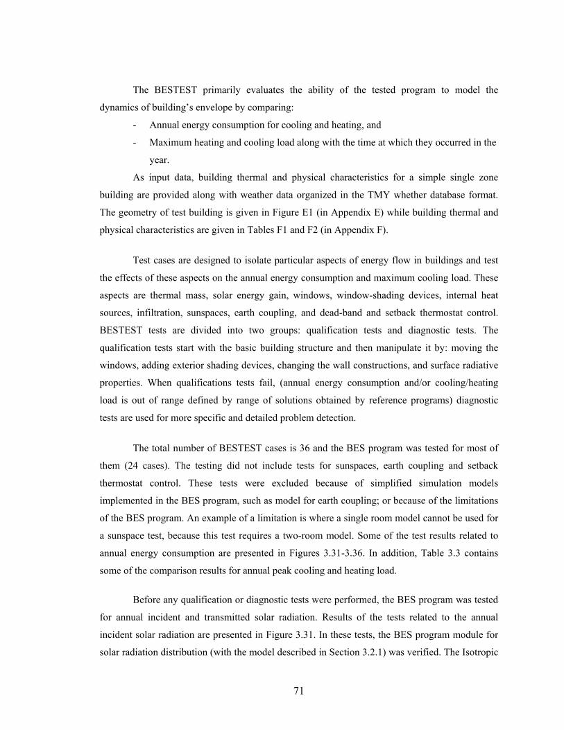
71

The BESTEST primarily evaluates the ability of the tested program to model the

dynamics of building’s envelope by comparing:

- Annual energy consumption for cooling and heating, and

- Maximum heating and cooling load along with the time at which they occurred in the

year.

As input data, building thermal and physical characteristics for a simple single zone

building are provided along with weather data organized in the TMY whether database format.

The geometry of test building is given in Figure E1 (in Appendix E) while building thermal and

physical characteristics are given in Tables F1 and F2 (in Appendix F).

Test cases are designed to isolate particular aspects of energy flow in buildings and test

the effects of these aspects on the annual energy consumption and maximum cooling load. These

aspects are thermal mass, solar energy gain, windows, window-shading devices, internal heat

sources, infiltration, sunspaces, earth coupling, and dead-band and setback thermostat control.

BESTEST tests are divided into two groups: qualification tests and diagnostic tests. The

qualification tests start with the basic building structure and then manipulate it by: moving the

windows, adding exterior shading devices, changing the wall constructions, and surface radiative

properties. When qualifications tests fail, (annual energy consumption and/or cooling/heating

load is out of range defined by range of solutions obtained by reference programs) diagnostic

tests are used for more specific and detailed problem detection.

The total number of BESTEST cases is 36 and the BES program was tested for most of

them (24 cases). The testing did not include tests for sunspaces, earth coupling and setback

thermostat control. These tests were excluded because of simplified simulation models

implemented in the BES program, such as model for earth coupling; or because of the limitations

of the BES program. An example of a limitation is where a single room model cannot be used for

a sunspace test, because this test requires a two-room model. Some of the test results related to

annual energy consumption are presented in Figures 3.31-3.36. In addition, Table 3.3 contains

some of the comparison results for annual peak cooling and heating load.

Before any qualification or diagnostic tests were performed, the BES program was tested

for annual incident and transmitted solar radiation. Results of the tests related to the annual

incident solar radiation are presented in Figure 3.31. In these tests, the BES program module for

solar radiation distribution (with the model described in Section 3.2.1) was verified. The Isotropic

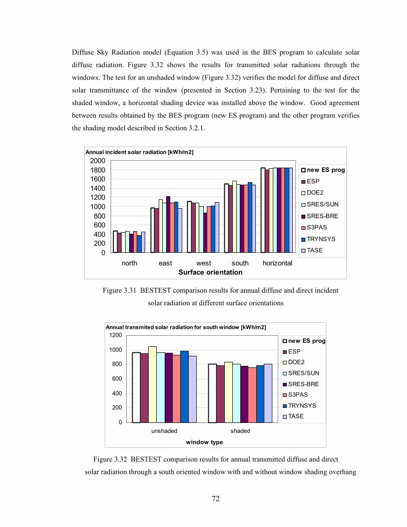
72

Diffuse Sky Radiation model (Equation 3.5) was used in the BES program to calculate solar

diffuse radiation. Figure 3.32 shows the results for transmitted solar radiations through the

windows. The test for an unshaded window (Figure 3.32) verifies the model for diffuse and direct

solar transmittance of the window (presented in Section 3.23). Pertaining to the test for the

shaded window, a horizontal shading device was installed above the window. Good agreement

between results obtained by the BES program (new ES program) and the other program verifies

the shading model described in Section 3.2.1.

Annual incident solar radiation [kWh/m2]

0200400600800

100012001400160018002000

north east west south horizontalSurface orientation

new ES prog

ESP

DOE2

SRES/SUN

SRES-BRE

S3PAS

TRYNSYS

TASE

Figure 3.31 BESTEST comparison results for annual diffuse and direct incident

solar radiation at different surface orientations

Annual transmited solar radiation for south window [kWh/m2]

0

200

400

600

800

1000

1200

unshaded shaded

window type

new ES prog

ESP

DOE2

SRES/SUN

SRES-BRE

S3PAS

TRYNSYS

TASE

Figure 3.32 BESTEST comparison results for annual transmitted diffuse and direct

solar radiation through a south oriented window with and without window shading overhang

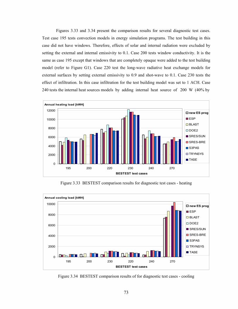
73

Figures 3.33 and 3.34 present the comparison results for several diagnostic test cases.

Test case 195 tests convection models in energy simulation programs. The test building in this

case did not have windows. Therefore, effects of solar and internal radiation were excluded by

setting the external and internal emissivity to 0.1. Case 200 tests window conductivity. It is the

same as case 195 except that windows that are completely opaque were added to the test building

model (refer to Figure G1). Case 220 test the long-wave radiative heat exchange models for

external surfaces by setting external emissivity to 0.9 and shot-wave to 0.1. Case 230 tests the

effect of infiltration. In this case infiltration for the test building model was set to 1 ACH. Case

240 tests the internal heat sources models by adding internal heat source of 200 W (40% by

BESTEST test cases

0

2000

4000

6000

8000

10000

12000

195 200 220 230 240 270

Annual heating load [kWH]

new ES prog

ESP

BLAST

DOE2

SRES/SUN

SRES-BRE

S3PAS

TRYNSYS

TASE

Figure 3.33 BESTEST comparison results for diagnostic test cases - heating

BESTEST test cases

0

2000

4000

6000

8000

10000

195 200 230 220 240 270

Annual cooling load [kWH]

new ES prog

ESP

BLAST

DOE2

SRES/SUN

SRES-BRE

S3PAS

TRYNSYS

TASE

Figure 3.34 BESTEST comparison results of for diagnostic test cases - cooling

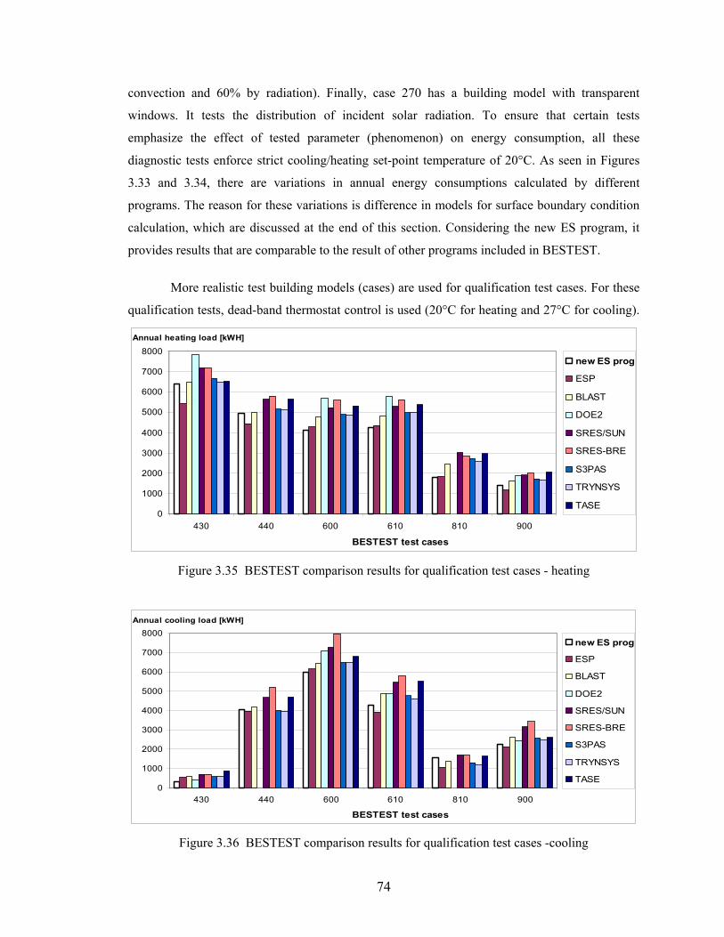
74

convection and 60% by radiation). Finally, case 270 has a building model with transparent

windows. It tests the distribution of incident solar radiation. To ensure that certain tests

emphasize the effect of tested parameter (phenomenon) on energy consumption, all these

diagnostic tests enforce strict cooling/heating set-point temperature of 20°C. As seen in Figures

3.33 and 3.34, there are variations in annual energy consumptions calculated by different

programs. The reason for these variations is difference in models for surface boundary condition

calculation, which are discussed at the end of this section. Considering the new ES program, it

provides results that are comparable to the result of other programs included in BESTEST.

More realistic test building models (cases) are used for qualification test cases. For these

qualification tests, dead-band thermostat control is used (20°C for heating and 27°C for cooling).

BESTEST test cases

0

1000

2000

3000

4000

5000

6000

7000

8000

430 440 600 610 810 900

Annual heating load [kWH]

new ES prog

ESP

BLAST

DOE2

SRES/SUN

SRES-BRE

S3PAS

TRYNSYS

TASE

Figure 3.35 BESTEST comparison results for qualification test cases - heating

BESTEST test cases

0

1000

2000

3000

4000

5000

6000

7000

8000

430 440 600 610 810 900

Annual cooling load [kWH]

new ES prog

ESP

BLAST

DOE2

SRES/SUN

SRES-BRE

S3PAS

TRYNSYS

TASE

Figure 3.36 BESTEST comparison results for qualification test cases -cooling

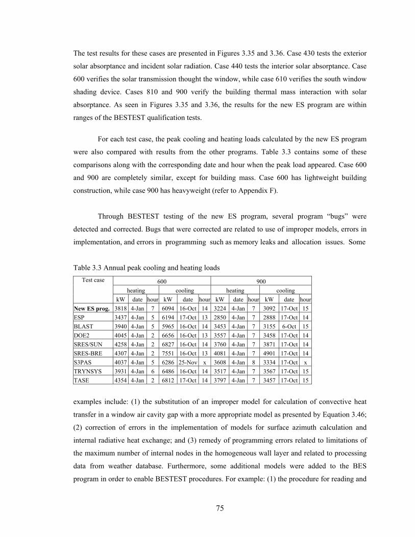
75

The test results for these cases are presented in Figures 3.35 and 3.36. Case 430 tests the exterior

solar absorptance and incident solar radiation. Case 440 tests the interior solar absorptance. Case

600 verifies the solar transmission thought the window, while case 610 verifies the south window

shading device. Cases 810 and 900 verify the building thermal mass interaction with solar

absorptance. As seen in Figures 3.35 and 3.36, the results for the new ES program are within

ranges of the BESTEST qualification tests.

For each test case, the peak cooling and heating loads calculated by the new ES program

were also compared with results from the other programs. Table 3.3 contains some of these

comparisons along with the corresponding date and hour when the peak load appeared. Case 600

and 900 are completely similar, except for building mass. Case 600 has lightweight building

construction, while case 900 has heavyweight (refer to Appendix F).

Through BESTEST testing of the new ES program, several program “bugs” were

detected and corrected. Bugs that were corrected are related to use of improper models, errors in

implementation, and errors in programming such as memory leaks and allocation issues. Some

Table 3.3 Annual peak cooling and heating loads

600 900 heating cooling heating cooling

Test case

kW date hour kW date hour kW date hour kW date hour New ES prog. 3818 4-Jan 7 6094 16-Oct 14 3224 4-Jan 7 3092 17-Oct 15 ESP 3437 4-Jan 5 6194 17-Oct 13 2850 4-Jan 7 2888 17-Oct 14 BLAST 3940 4-Jan 5 5965 16-Oct 14 3453 4-Jan 7 3155 6-Oct 15 DOE2 4045 4-Jan 2 6656 16-Oct 13 3557 4-Jan 7 3458 17-Oct 14 SRES/SUN 4258 4-Jan 2 6827 16-Oct 14 3760 4-Jan 7 3871 17-Oct 14 SRES-BRE 4307 4-Jan 2 7551 16-Oct 13 4081 4-Jan 7 4901 17-Oct 14 S3PAS 4037 4-Jan 5 6286 25-Nov x 3608 4-Jan 8 3334 17-Oct x TRYNSYS 3931 4-Jan 6 6486 16-Oct 14 3517 4-Jan 7 3567 17-Oct 15 TASE 4354 4-Jan 2 6812 17-Oct 14 3797 4-Jan 7 3457 17-Oct 15

examples include: (1) the substitution of an improper model for calculation of convective heat

transfer in a window air cavity gap with a more appropriate model as presented by Equation 3.46;

(2) correction of errors in the implementation of models for surface azimuth calculation and

internal radiative heat exchange; and (3) remedy of programming errors related to limitations of

the maximum number of internal nodes in the homogeneous wall layer and related to processing

data from weather database. Furthermore, some additional models were added to the BES

program in order to enable BESTEST procedures. For example: (1) the procedure for reading and

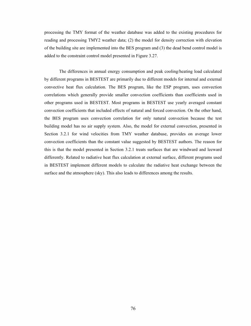
76

processing the TMY format of the weather database was added to the existing procedures for

reading and processing TMY2 weather data; (2) the model for density correction with elevation

of the building site are implemented into the BES program and (3) the dead bend control model is

added to the constraint control model presented in Figure 3.27.

The differences in annual energy consumption and peak cooling/heating load calculated

by different programs in BESTEST are primarily due to different models for internal and external

convective heat flux calculation. The BES program, like the ESP program, uses convection

correlations which generally provide smaller convection coefficients than coefficients used in

other programs used in BESTEST. Most programs in BESTEST use yearly averaged constant

convection coefficients that included effects of natural and forced convection. On the other hand,

the BES program uses convection correlation for only natural convection because the test

building model has no air supply system. Also, the model for external convection, presented in

Section 3.2.1 for wind velocities from TMY weather database, provides on average lower

convection coefficients than the constant value suggested by BESTEST authors. The reason for

this is that the model presented in Section 3.2.1 treats surfaces that are windward and leeward

differently. Related to radiative heat flux calculation at external surface, different programs used

in BESTEST implement different models to calculate the radiative heat exchange between the

surface and the atmosphere (sky). This also leads to differences among the results.

77

3.6 Summary

This chapter has described physical and numerical models that have been implemented

into the newly developed BES program. Using these models, the BES program is capable of

precisely calculating heat flow within a room with or without a plenum above it. The primary

reason for the development of BES was to couple it with the airflow program. Therefore, during

the BES program development, the focus was on the implementation of heat transfer models

which enable accurate calculations of internal surface temperatures that are necessary for

coupling.

This chapter has also described a new method for simultaneous load calculation and

HVAC system simulation that was developed as part of the BES program. This new method has

certain advantages over procedures used in the ESP-r and EnergyPlus programs. This method

enables modular organization of HVAC system models because HVAC equations are NOT

integrated into the zone matrix. On the other hand, this method calculates enclosure temperatures

and energy stored in building elements because it uses a “predictor-corrector” method to correct

all temperatures in the energy simulation domain. In this way, the new method enables better

prediction of thermal comfort and HVAC system performance. This is especially so in the case

with systems where building thermal storage has a large influence on energy flow, such as

heating/cooling slabs and systems with radiant panels.

Finally, this chapter has described extensive validation procedures that were performed

during the program code development. The good validation results showed that the BES program

can be coupled with the airflow program. Furthermore, BESTEST results demonstrate that the

BES program can be used in various analyses related to energy consumption in buildings. Also,

good validation results of the current version of BES demonstrate that the program is ready for

further development. This can be done by: (1) adding procedures that will increase the number of

rooms that can be analyzed (multizone building); (2) adding different HVAC system models that

use the proposed coupling method for simultaneous load calculation and HVAC system

simulation.

78

CHAPTER 4

AIR FLOW PROGRAM - BOUNDARY CONDITIONS

4.1 Introduction

As described in Chapter 2, Computation Fluid Dynamics (CFD) programs have been

successfully used as indoor air flow programs. They provide detailed information about air

velocity, temperature, and contaminant concentration in buildings. Hence, a CFD program was

selected as the airflow simulation tool for coupling with the building energy simulation (BES)

program. The CFD programs are used in a wide range of scientific and engineering fields.

Therefore, there is a large number of well-established research and commercial CFD software

packages. The BES program has been coupled with a CFD program called CFD0, which was

developed for research purposes at the Massachusetts Institute of Technology (MIT) (Srebric

2000). This program was extensively validated by the developer (Srebric 2000). Because of the

necessity to modify the CFD source code for effective coupling with the BES program, priority

was given to this CFD program over the other commercial codes that had larger variety of

implemented turbulence models and more extensive validation, but provided none or very limited

access to their respective source codes. The CFD0 program has certain limitations (these will be

described later) and therefore for the particular analysis in this thesis, the PHOENICS commercial

CFD package (CHAM 2004) is used in addition to the existing program. Chapter 1 pointed out that the coupling of the ES and CFD programs takes place at the

surfaces of simulation domains. Therefore, it is critical that CFD models accurately calculate the

convective heat transfer on the envelope surfaces. Consequently, the focus of this chapter, besides

the coupling interface, is the modification of the CFD0 program by implementation of newly

developed convection correlations. The aim of this undertaking was to accurately calculate the

surface convective heat flux. An understanding of the CFD’s theoretical fundamentals is

necessary in order to explore these issues. Therefore, Section 4.2 provides the conceptual basis of

CFD programs, used numerical models, and the relevant equation solver. Readers interested only

in new models for thermal boundary condition calculations in the CFD program can directly go to

Section 3.4. This section provides information about the implementation of experiment-based

convection correlations in CFD. Section 4.5 shows the validation of these new models for thermal

boundaries in CFD. Finally, Section 4.6 concludes the chapter with a discussion and summary.

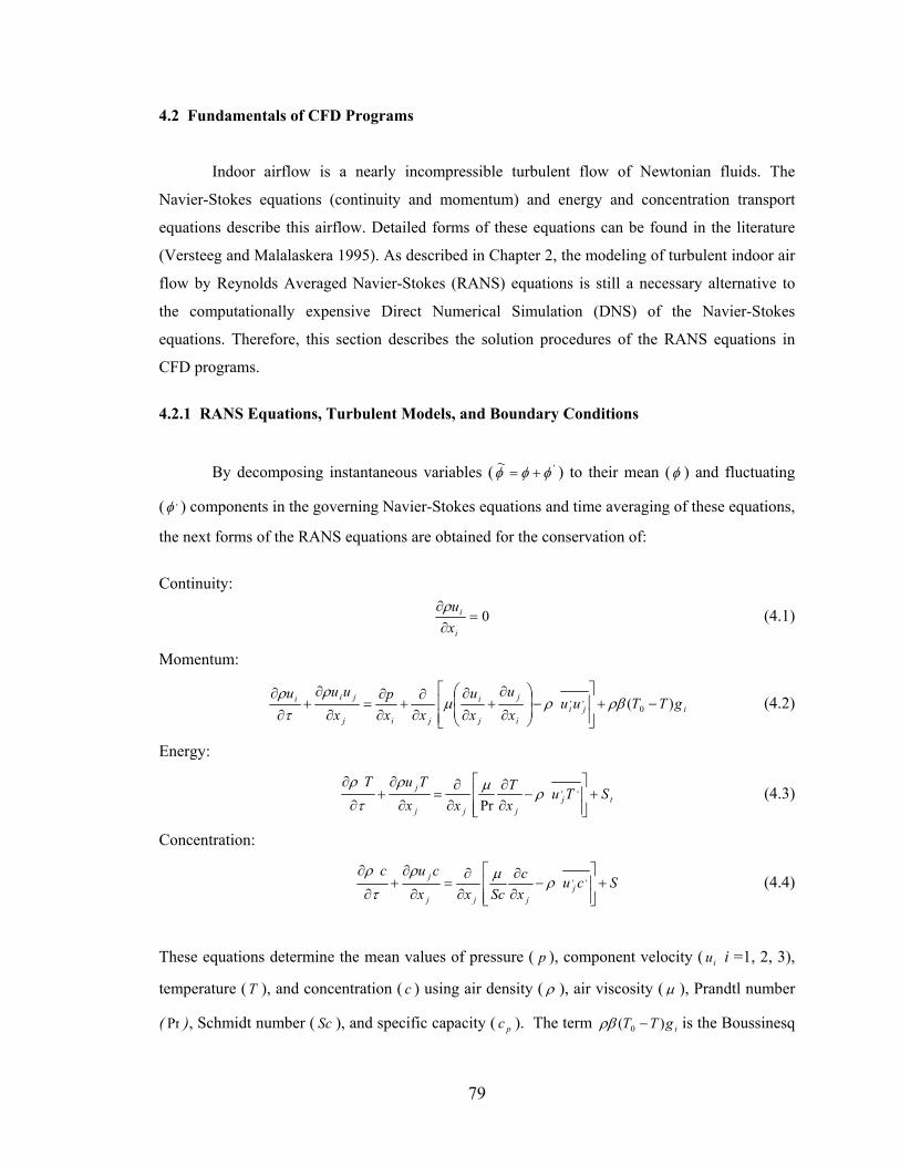
79

4.2 Fundamentals of CFD Programs

Indoor airflow is a nearly incompressible turbulent flow of Newtonian fluids. The

Navier-Stokes equations (continuity and momentum) and energy and concentration transport

equations describe this airflow. Detailed forms of these equations can be found in the literature

(Versteeg and Malalaskera 1995). As described in Chapter 2, the modeling of turbulent indoor air

flow by Reynolds Averaged Navier-Stokes (RANS) equations is still a necessary alternative to

the computationally expensive Direct Numerical Simulation (DNS) of the Navier-Stokes

equations. Therefore, this section describes the solution procedures of the RANS equations in

CFD programs.

4.2.1 RANS Equations, Turbulent Models, and Boundary Conditions

By decomposing instantaneous variables ( '~φφφ += ) to their mean (φ ) and fluctuating

( ,φ ) components in the governing Navier-Stokes equations and time averaging of these equations,

the next forms of the RANS equations are obtained for the conservation of:

Continuity:

0=∂

∂

i

i

xuρ (4.1)

Momentum:

ijii

j

j

i

jij

jii gTTuuxu

xu

xxp

xuuu

)( 0,, −+

−

∂

∂+

∂∂

∂∂

+∂∂

=∂

∂+

∂∂

ρβρµρ

τρ (4.2)

Energy:

tjjjj

j STuxT

xxTuT

+

−

∂∂

∂∂

=∂

∂+

∂

∂ ,,

Prρµρ

τρ

(4.3)

Concentration:

Scuxc

Scxxcuc

jjjj

j +

−

∂∂

∂∂

=∂

∂+

∂

∂ ,,ρµρτ

ρ (4.4)

These equations determine the mean values of pressure ( p ), component velocity ( iu i =1, 2, 3),

temperature ( T ), and concentration ( c ) using air density ( ρ ), air viscosity ( µ ), Prandtl number

( Pr ), Schmidt number ( Sc ), and specific capacity ( pc ). The term igTT )( 0 −ρβ is the Boussinesq

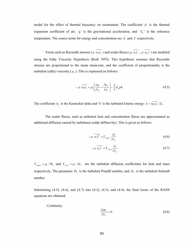
80

model for the effect of thermal buoyancy on momentum. The coefficient β is the thermal

expansion coefficient of air, ‘ g’ is the gravitational acceleration, and ‘ 0T ’ is the reference

temperature. The source terms for energy and concentration are tS and S respectively.

Terms such as Reynolds stresses ( ,,jiuuρ ) and scalar fluxes ( ,, tu jρ , ,, cu jρ ) are modeled

using the Eddy Viscosity Hypothesis (Rodi 1993). This hypothesis assumes that Reynolds

stresses are proportional to the mean strain-rate, and the coefficient of proportionality is the

turbulent (eddy) viscosity ( tµ ). This is expressed as follows:

kxu

xu

uu iji

j

j

itji ρδµρ

32,, −

∂

∂+

∂∂

=− (4.5)

The coefficient ijδ is the Kronecker delta and ‘k’ is the turbulent kinetic energy: )2/( iiuuk = .

The scalar fluxes, such as turbulent heat and concentration fluxes are approximated as

additional diffusion caused by turbulence (eddy-diffusivity). This is given as follows:

jttempi x

tTu∂∂

Γ=− ,,,ρ (4.6)

jtconi x

ccu∂∂

Γ=− ,,,ρ (4.7)

ttttemp Pr/, µ=Γ and tttcon Sc/, µ=Γ are the turbulent diffusion coefficients for heat and mass

respectively. The parameter tPr is the turbulent Prandtl number, and tSc is the turbulent Schmidt

number.

Substituting (4.5), (4.6), and (4.7) into (4.2), (4.3), and (4.4), the final forms of the RANS

equations are obtained:

- Continuity:

0=∂

∂

i

i

xuρ (4.8)

81

- Momentum:

ii

j

j

ieff

jij

jii gTTxu

xu

xxp

xuuu

)( 0 −+

∂

∂+

∂∂

∂∂

+∂∂

=∂

∂+

∂∂

ρβµρ

τρ (4.9)

- Energy:

pjefftemp

jj

j

cq

xT

xxTuT

+

∂∂

Γ∂∂

=∂

∂+

∂

∂,

ρτ

ρ (4.10)

- Concentration:

sj

effconjj

j Cxc

xxcuc

ρρ

τρ

+

∂∂

Γ∂∂

=∂

∂+

∂

∂, (4.11)

The influence of turbulence is integrated into the effective viscosity as the sum of the

turbulent and laminar viscosity µµµ += teff . The effective diffusion coefficient for heat

(temperature) is proportional to the effective viscosity effeffefftemp Pr/, µ=Γ since the eddy mixing is

a source of turbulent diffusivity ( ttefftemp Pr/Pr/, µµ +=Γ ). The same relation holds for the effective

diffusion coefficient for mass (concentration). This is given as: tteffeffeffcon ScScSc ///, µµµ +==Γ .

Zero Equation Turbulence Model

The zero-equation turbulence models are eddy viscosity models in which the turbulent

viscosity is represented by an algebraic equation. These models use a fixed value for the eddy

viscosity or relate it to the mean-velocity distribution. In 1925, Prandtl (Rodi 1993) provided the

basis for zero-equation models by introducing the mixing-length hypothesis. Forming an analogy

with the molecular transport of momentum, Prandtl postulated the mixing-length hypothesis in

the following form:

dydulmixt

2⋅= ρµ (4.12)

where lmix is the mixing length, ρ is the fluid density, and u is the average velocity.

The mixing length is a characteristic property of the flow field. The product of the mixing

length and the velocity gradient is called the mixing velocity. This is also a property of turbulent

flows. Prandtl (Rodi 1993) assumed that the mixing length near solid surfaces is proportional to

the distance from the surface. This approximation gives good results for a certain class of

82

turbulent boundary layers such as free shear flows. However, calibration of the mixing length is

always needed for complex flows (Wilcox 1993).

Considerable effort has been made to extend the applicability of the mixing length model

(Rodi 1993). An example is a research project conducted by Chen and Xu (1998) who developed

zero equation models for room airflows which are primarily buoyancy-driven flows. As the basis

for this new model, they used the Prandtl-Kolmogorov assumption, which states that the turbulent

viscosity is the product of turbulent kinetic energy (k) and length scale for turbulence interactions

(l). This is given as follows:

lkCvt

2/1⋅⋅= ρµ (4.13)

The coefficient Cν = 0.5478 is an empirical constant. Chen and Xu (1998) introduced additional

assumptions related to turbulent kinetic energy using the relation between kinetic energy

turbulence intensity Ti and mean airflow velocity ‘u’. This is given as:

uk

uu

T ii

22,

== (4.14)

Chen and Xu assumed a uniform turbulence intensity and derived an algebraic function to express

the turbulent viscosity as a function of the local mean velocity (U) and length scale (l). This is

given as follows:

luTi

t2

5487.0 ρµ = (4.15)

Substituting T i= 0.1, the final form of the new empirical zero equation model is obtained:

ult ρµ 03874.0= (4.16)

The empirical constant (0.03874) is a universal value for different room airflows. The length

scale (l) is the distance to the closest surface of the enclosure and u is the local velocity.

The assumption, that the turbulence intensity for indoor airflow is uniform is a good

estimate for the occupied zone and mixing ventilation. However, this assumption can differ

considerably from reality in the jet region. To evaluate model performance, Chen and Xu (1998)

presented simulation results for four room airflows with mostly two dimensional airflows. The

83

results showed good agreements between the zero-equation model predictions and the

experimental data. Srebric et al. (1999) provided further validation of this turbulent model for

three dimensional cases. They compared the zero-equation model’s predictions to experimental

data for three cases of room airflow: natural convection with infiltration, forced convection, and

mixed convection with displacement ventilation. This second validation study found good

agreements between the calculated and measured values for air velocity and temperature

distribution.

k-ε turbulence model

Another approach to model turbulent viscosity is the use of two additional transport

equations that model turbulence kinetic energy (k) and the dissipation rate of turbulence energy

(ε). With this model, the turbulent viscosity is evaluated without assumptions regarding length

scale. This is given as follows:

ερµ µ

2kCt = (4.17)

The coefficient Cµ = 0.09 is an empirical constant.

The equations that calculate local distributions of k and ε are derived from the Navier-

Stokes equations (Rodi 1993). The following are equations for kinetic and turbulence energy:

Turbulence kinetic energy:

it

t

i

j

j

i

j

it

jeff

jj

i

xT

gxu

xu

xu

xk

xxkuk

∂∂µ

βρε∂∂

∂∂

∂∂

µµρ

τρ

Pr−−

+⋅+

∂∂

∂∂

=∂

∂+

∂∂ (4.18)

Dissipation rate of turbulence energy:

it

t

i

j

j

i

j

it

jeff

jj

i

xT

gk

Ck

Cxu

xu

xu

kC

xxxu

∂∂µ

βεερ∂∂

∂∂

∂∂

µεεµερ

τρε

Pr1

2

21 −−

+⋅+

∂∂

∂∂

=∂

∂+

∂∂ (4.19)

Empirical constants σk, σε, C1, and C2 are experimentally determined for certain types of flow.

There are many variations of the k - ε model depending on the values of the empirical

constants and modifications of terms in equations (4.18) and (4.19). Chen (1995) evaluated the

performance of five k-ε models: the standard k-ε model (Launder and Spalding 1974), a low-

Reynolds-number k-ε model, a two-layer k-ε model, a two-scale k-ε model, and a renormalization

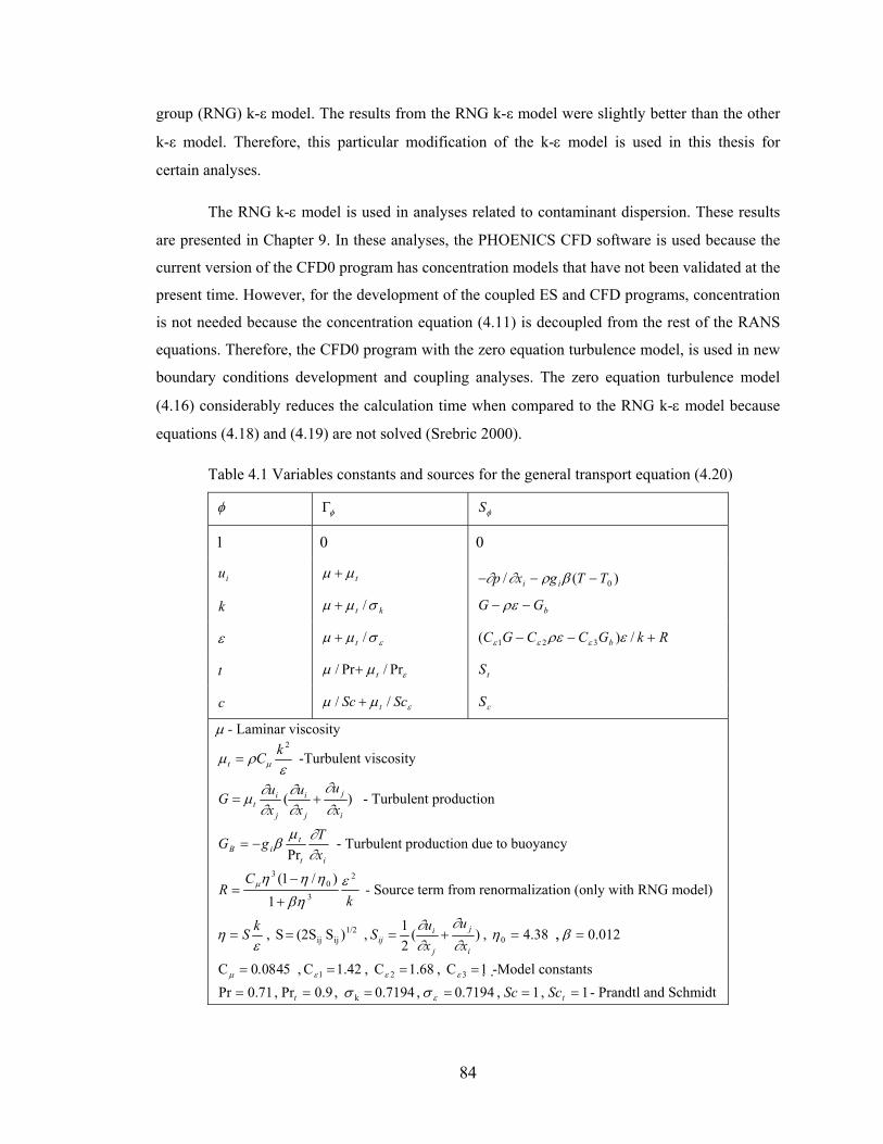
84

group (RNG) k-ε model. The results from the RNG k-ε model were slightly better than the other

k-ε model. Therefore, this particular modification of the k-ε model is used in this thesis for

certain analyses.

The RNG k-ε model is used in analyses related to contaminant dispersion. These results

are presented in Chapter 9. In these analyses, the PHOENICS CFD software is used because the

current version of the CFD0 program has concentration models that have not been validated at the

present time. However, for the development of the coupled ES and CFD programs, concentration

is not needed because the concentration equation (4.11) is decoupled from the rest of the RANS

equations. Therefore, the CFD0 program with the zero equation turbulence model, is used in new

boundary conditions development and coupling analyses. The zero equation turbulence model

(4.16) considerably reduces the calculation time when compared to the RNG k-ε model because

equations (4.18) and (4.19) are not solved (Srebric 2000). Table 4.1 Variables constants and sources for the general transport equation (4.20)

φ φΓ φS

1 0 0

iu tµµ + )(/ 0TTgxp ii −−− βρ∂∂

k kt σµµ / + bGG −− ρε

ε εσµµ /t + RkGCCGC b +−− /)( 321 ερε εεε

t εµµ Pr/Pr/ t + tS

c εµµ ScSc t // + cS

µ - Laminar viscosity

ερµ µ

2kCt = -Turbulent viscosity

)(i

j

j

i

j

it x

uxu

xuG

∂∂

∂∂

∂∂µ += - Turbulent production

it

tiB x

TgG∂∂µ

βPr

−= - Turbulent production due to buoyancy

kC

R2

30

3

1)/1( ε

βηηηηµ

+

−= - Source term from renormalization (only with RNG model)

εη kS= , 1/2

ijij )S (2S S = , )(21

i

j

j

iij x

uxuS

∂∂

∂∂

+= , 38.40 =η , 012.0=β

0.0845= Cµ , 1.42 C 1 =ε , 1.68 C 2 =ε , 1 C 3 =ε -Model constants 71.0Pr = , 9.0Pr =t , 0.7194 k =σ , 0.7194 =εσ , 1=Sc , 1=tSc - Prandtl and Schmidt

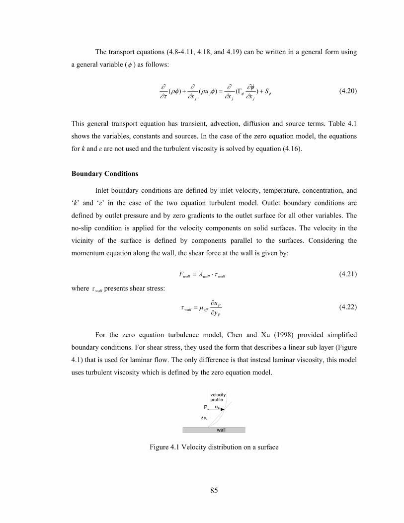
85

The transport equations (4.8-4.11, 4.18, and 4.19) can be written in a general form using

a general variable (φ ) as follows:

φφ ∂∂φ

∂∂φρ

∂∂ρφ

∂τ∂ S

xxu

x jjj

j

+Γ=+ )()()( (4.20)

This general transport equation has transient, advection, diffusion and source terms. Table 4.1

shows the variables, constants and sources. In the case of the zero equation model, the equations

for k and ε are not used and the turbulent viscosity is solved by equation (4.16).

Boundary Conditions Inlet boundary conditions are defined by inlet velocity, temperature, concentration, and

‘k’ and ‘ε’ in the case of the two equation turbulent model. Outlet boundary conditions are

defined by outlet pressure and by zero gradients to the outlet surface for all other variables. The

no-slip condition is applied for the velocity components on solid surfaces. The velocity in the

vicinity of the surface is defined by components parallel to the surfaces. Considering the

momentum equation along the wall, the shear force at the wall is given by:

wallwallwall AF τ⋅= (4.21)

where wallτ presents shear stress:

P

Peffwall y

u∂∂

= µτ (4.22)

For the zero equation turbulence model, Chen and Xu (1998) provided simplified

boundary conditions. For shear stress, they used the form that describes a linear sub layer (Figure

4.1) that is used for laminar flow. The only difference is that instead laminar viscosity, this model

uses turbulent viscosity which is defined by the zero equation model.

P

velocity profile

uP

∆yP

wall

Figure 4.1 Velocity distribution on a surface

86

Convective heat transfer is defined by the temperature difference between the air in the

vicinity of the surface ( PT ) and surface temperature ( wallT ) as follows:

)( wallPwall TThq −= (4.23)

The local convection coefficient (h) is defined by effective diffusivity ( efftemp,Γ ) as follows:

P

pefftemp y

ch

∆Γ= , (4.24)

These simplified boundary conditions are grid dependent and, therefore, inaccurate,

especially for buoyancy-driven flows (Beausoleil 2000). The reason for the good agreement

between experimental and numerical results during the validation of the zero equation models by

Srebric et al. (1999) is that convective heat fluxes ( wallq ) on surfaces are provided based on

experimental measurements.

Boundary conditions models that use log-low wall functions have slightly better

accuracy. This model is typically used with k-ε models. The previously described RNG k-ε model

is valid for high Reynolds number turbulent flows. Therefore, wall functions are needed for the

region near walls where the Reynolds number is low. The wall functions asume a velocity

distribution near a solid wall. This velocity profile is usually described by dimensionless velocity

(u+) and dimensionless distance from the wall (y+) for several regions of the boundary layer.

These are given as follows:

- Laminar sub-layer: ++ = yu for 0< y+ ≤5 (4.25)

- Log-law layer: )ln(/1 ++ ⋅= Eyu κ for 30 <y+ ≤500 (4.26)

The 41.0=κ is the Karman constant and 9.8E = is an integration constant. The layer closest to

the wall (laminar sub-layer) has dominant viscous forces, while the log-law layer has dominant

turbulent forces. In-between these, lies the buffer zone where viscous forces and Reynolds

stresses have the same order of magnitude. Depending on the position of first grid cell (adjacent

to the wall) in boundary layer, the wall function algorithm selects an appropriate equation and

87

calculates wallτ and wallq based on local velocity, temperature, and kinetic energy. Details about

the calculation of wallτ and wallq are provided in the literature (Versteeg and Malalaskera 1995).

Similar to simplified boundary conditions, log-law wall functions are grid-dependent

(Chen and Jiang 1992). Generally, the log-law wall functions under-predict the heat flux on

building surfaces. Depending on grid size in the vicinity of the surface convective heat flux might

be several times smaller/larger. Log-law wall functions are good for boundary condition

calculations only on surfaces where the Grashof-Reynolds ratio Gr/Re2<<1 and the turbulent-

laminar viscosity ratio: µt /µ>30 (Beausoleil 2000). This means that the log-law wall functions are

applicable only on surfaces of the room that are in the vicinity of the supply diffuser, where the

air velocity is large. Therefore, in this thesis neither simplified boundary conditions (used with

new zero equation model) nor log-law wall functions are used for the calculation of thermal

boundary conditions. Instead, experiment-based convection correlations are used. Details about

these correlations are provided in Section 4.3.

4.2.2 Numerical Discretization

The RANS equations (4.1-4.4) create a non-linear system of equations. The diffusion

term in the general transport equation (4.20) is a non-linear term. Also, the RANS equations are

connected because of three reasons. First, each momentum equation contains all three velocity

components; second, temperature appears in the momentum equation; and third, the energy

equation contains the velocity components. Therefore, these equations can be solved analytically

only for simple problems.

In order to use the numerical method, room air, which is the simulation domain of CFD

program, needs to be discretized. Discretization transforms the partial differential equations into a

system of algebraic equations which describe conservations of mass, momentum, energy,

concentration, kinetic energy, and dissipation for each cell of discretized space. Using the finite

volume method, the room is divided into a finite number of volumes using a grid system (Figure

4.2). Variables are calculated at discrete points located at the centers of these finite volumes, with

the exception of velocities that are solved at volume surfaces in order to solve the problems

related to linking the pressure and velocity solutions (Versteeg and Malalasekera 1995).

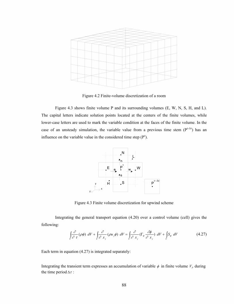
88

Figure 4.2 Finite-volume discretization of a room

Figure 4.3 shows finite volume P and its surrounding volumes (E, W, N, S, H, and L).

The capital letters indicate solution points located at the centers of the finite volumes, while

lower-case letters are used to mark the variable condition at the faces of the finite volume. In the

case of an unsteady simulation, the variable value from a previous time stem (Pτ-∆τ) has an

influence on the variable value in the considered time step (Pτ).

N

S

We

n

s

wE

H

L

x

y

z

Pτ−∆τ

Pτ

Figure 4.3 Finite volume discretization for upwind scheme Integrating the general transport equation (4.20) over a control volume (cell) gives the

following:

∫∫∫∫ +Γ=+VV jjV

jjV

dVSdVxx

dVux

dV φφ ∂∂φ

∂∂φρ

∂∂ρφ

τ∂∂ )()()( (4.27)

Each term in equation (4.27) is integrated separately:

Integrating the transient term expresses an accumulation of variable φ in finite volume PV during the time period τ∆ :

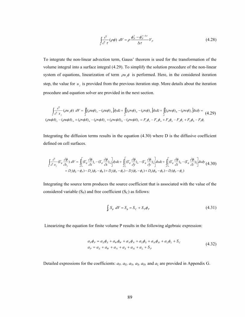
89

PPP

V

VdVτφφ

ρρφτ∂

∂ τττ

∆−

=∆−

∫ )( (4.28)

To integrate the non-linear advection term, Gauss’ theorem is used for the transformation of the

volume integral into a surface integral (4.29). To simplify the solution procedure of the non-linear

system of equations, linearization of term φρ ju is performed. Here, in the considered iteration

step, the value for ju is provided from the previous iteration step. More details about the iteration

procedure and equation solver are provided in the next section.

[ ] [ ] [ ]

llhhssnnwweelhsnwe

Alh

Asn

Awe

Vj

j

FFFFFFAwAwAvAvAuAu

dxdywwdxdzvvdydzuudVux

φφφφφφφρφρφρφρφρφρ

φρφρφρφρφρφρφρ∂

∂

−+−+−=−+−+−

=−+−+−= ∫∫∫∫)()()()()()(

)()()()()()()( (4.29)

Integrating the diffusion terms results in the equation (4.30) where D is the diffusive coefficient

defined on cell surfaces.

)()()()()()(

)()()()()()()(

LPlPHhSPsPNnWPwPEe

Alh

Asn

Awe

V jj

DDDDDD

dxdyzz

dxdzyy

dydzxx

dVxx

φφφφφφφφφφφφ

∂∂φ

∂∂φ

∂∂φ

∂∂φ

∂∂φ

∂∂φ

∂∂φ

∂∂

φφφφφφφ

−−−+−−−+−−−=

Γ−Γ+

Γ−Γ+

Γ−Γ=Γ ∫∫∫∫ (4.30)

Integrating the source term produces the source coefficient that is associated with the value of the

considered variable (SP) and free coefficient (SC) as follows:

PPCVSSSdVS φφφ +==∫ (4.31)

Linearizing the equation for finite volume P results in the following algebraic expression:

PLHSNWEP

CLLHHSSNNWWEEPP

SaaaaaaaSaaaaaaa

++++++=++++++= φφφφφφφ

(4.32)

Detailed expressions for the coefficients: aP, aE, aN, aS, aH, and aL are provided in Appendix G.

90

Solver

Discretization and linearization transform the complex linear and non-linear governing

differential equations into a set of simple algebraic relations. The next step is to solve this

algebraic system of equations. The iterative solution of the non-linear advection term (4.29)

mentioned previously, requires an iterative procedure. Also, the pressure field does not have a

general transport equation. Therefore the pressure source term in the momentum equations (refer

to Table 4.1) must be calculated indirectly. The pressure is calculated by connecting the

continuity equation with the momentum equations and creating a system of four equations with

four unknowns. The buoyant source term that connects temperature with the momentum

equations is calculated based on temperature values from the previous iteration step.

The calculation procedure used in the CFD0 and Phoenics programs uses a variation of

the Semi-Implicit Method for the Pressure-Linked Equations (SIMPLE) algorithm (Patankar and

Spalding 1972). This method is a variation of the predictor-corrector iterative procedures for

calculating the pressure field. The solution procedure starts with an initial estimate for pressure,

velocities, turbulent parameters, temperature, and concentration. Then, the estimated pressure

(p*) is used to calculate velocity components (u*) from the momentum equations. Next, the

pressure is corrected in such a way that the velocities satisfy the continuity equation. The correct

pressure, (p) is linked to the pressure correction term (p’). This is illustrated as follows:

*' ppp −= (4.33)

Since the velocity field is calculated using estimated pressures, a velocity-correction term is given

as:

*' uuu −= , *' vvv −= , *' www −= (4.34)

Using the assumption related to the SIMPLER modification of the SIMPLE algorithm (Versteeg

and Malalasekera 1995), the relation between the velocity and pressure is given as:

)(' ePnbP

ee pp

aaA

u −−

=∑

(4.35)

91

where Pa is given by equation (4.32) andnb

a∑ is the sum of neighboring coefficients.

Substituting the velocity correction into the mass continuity equation gives the pressure

correction equation in the same form as the general transport equation. This is given as follows:

CnbnbPP Spapa += ∑ '' (4.36)

The coefficient SC is the source term and represents the continuity imbalance because of the

incorrect velocity field ( lhsnweC mmmmmmS −+−+−= where ‘m’ is the mass flow in mass

continuity equation).

Knowing the pressure correction p’, values for the corrected pressure field p are

calculated. Then, the velocity corrections (equation 4.34) and velocity components are solved

accordingly. Finally, based on pressure and velocity fields, other scalar variables are calculated

for the considered iteration step.

Iterative solution procedures can be unstable because of the non-linearity of advection

terms in the transport equations (4.20). To control the rate of change for considered variables,

linear and false-time step relaxation methods are used. Both relaxation methods control the

change of variables during the iteration procedure. In this way, numerical instability is reduced.

The linear relaxation is based on a modification of the calculated variable ( nφ ) by the

value of the variable calculated in previous iteration step ( 1−nφ ). This is illustrated as follows:

1)1( −−+⋅= nnnew ff φφφ (4.37)

The coefficient f is the linear relaxation factor (value in-between 0 and 1) and newφ is the value of

variable that is used in next calculation step.

The false time step relaxation has the same form as the transient term given by Equation

(4.28):

92

cellF

nn

Vτφφρ

∆− −1

(4.38)

The coefficient Fτ∆ is the false time step relaxation factor. This term is added to both sides of the

general transport equation as the source term. In this way, the false time step relaxation does not

affect the final solution. Small values for Fτ∆ increase the term as illustrated in Equation (4.38).

This “ballast” on left and right side of general transport equation slows down the solution

procedure, but prevents the propagation of the instability caused by large variations of the

calculated variables during the iteration procedure. Large values for Fτ∆ speed up the calculation

procedure but increase instability of the iterative solution procedure.

The SIMPLE method and its variations are not the only methods for solving coupled non-

linear equations (RANS equations). There is another solution method which uses sparse linear

system solvers like the one that the BES program uses, instead of the iterative procedure. With

this method, the equations (4.8-4.11, 4.18, and 4.19) are structured for a Newton iterative method.

After calculating the underlying Jacobian matrix, the appropriate linear sparse system solver is

used. This method became more popular recently. However, available CFD programs (CFD0,

PHOENICS, and FLUENT) use semi-implicit methods (SIMPLE). Therefore, these methods are

considered in this thesis.

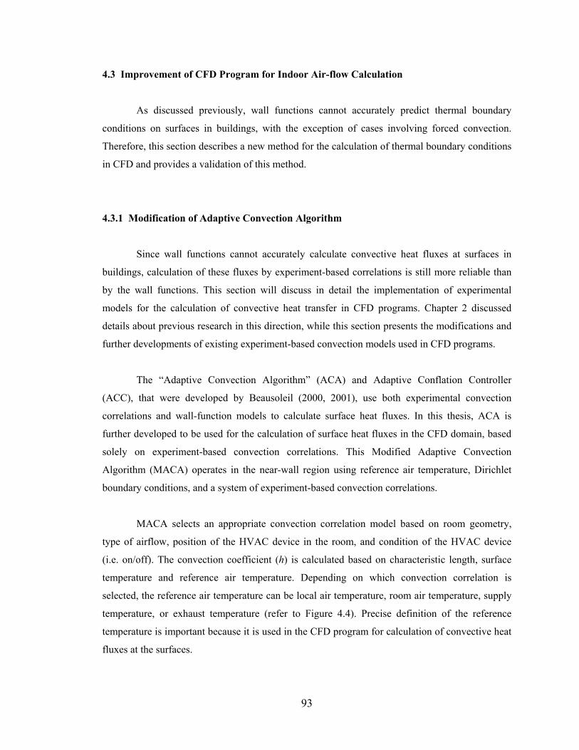
93

4.3 Improvement of CFD Program for Indoor Air-flow Calculation

As discussed previously, wall functions cannot accurately predict thermal boundary

conditions on surfaces in buildings, with the exception of cases involving forced convection.

Therefore, this section describes a new method for the calculation of thermal boundary conditions

in CFD and provides a validation of this method.

4.3.1 Modification of Adaptive Convection Algorithm

Since wall functions cannot accurately calculate convective heat fluxes at surfaces in

buildings, calculation of these fluxes by experiment-based correlations is still more reliable than

by the wall functions. This section will discuss in detail the implementation of experimental

models for the calculation of convective heat transfer in CFD programs. Chapter 2 discussed

details about previous research in this direction, while this section presents the modifications and

further developments of existing experiment-based convection models used in CFD programs.

The “Adaptive Convection Algorithm” (ACA) and Adaptive Conflation Controller

(ACC), that were developed by Beausoleil (2000, 2001), use both experimental convection

correlations and wall-function models to calculate surface heat fluxes. In this thesis, ACA is

further developed to be used for the calculation of surface heat fluxes in the CFD domain, based

solely on experiment-based convection correlations. This Modified Adaptive Convection

Algorithm (MACA) operates in the near-wall region using reference air temperature, Dirichlet

boundary conditions, and a system of experiment-based convection correlations.

MACA selects an appropriate convection correlation model based on room geometry,

type of airflow, position of the HVAC device in the room, and condition of the HVAC device

(i.e. on/off). The convection coefficient (h) is calculated based on characteristic length, surface

temperature and reference air temperature. Depending on which convection correlation is

selected, the reference air temperature can be local air temperature, room air temperature, supply

temperature, or exhaust temperature (refer to Figure 4.4). Precise definition of the reference

temperature is important because it is used in the CFD program for calculation of convective heat

fluxes at the surfaces.

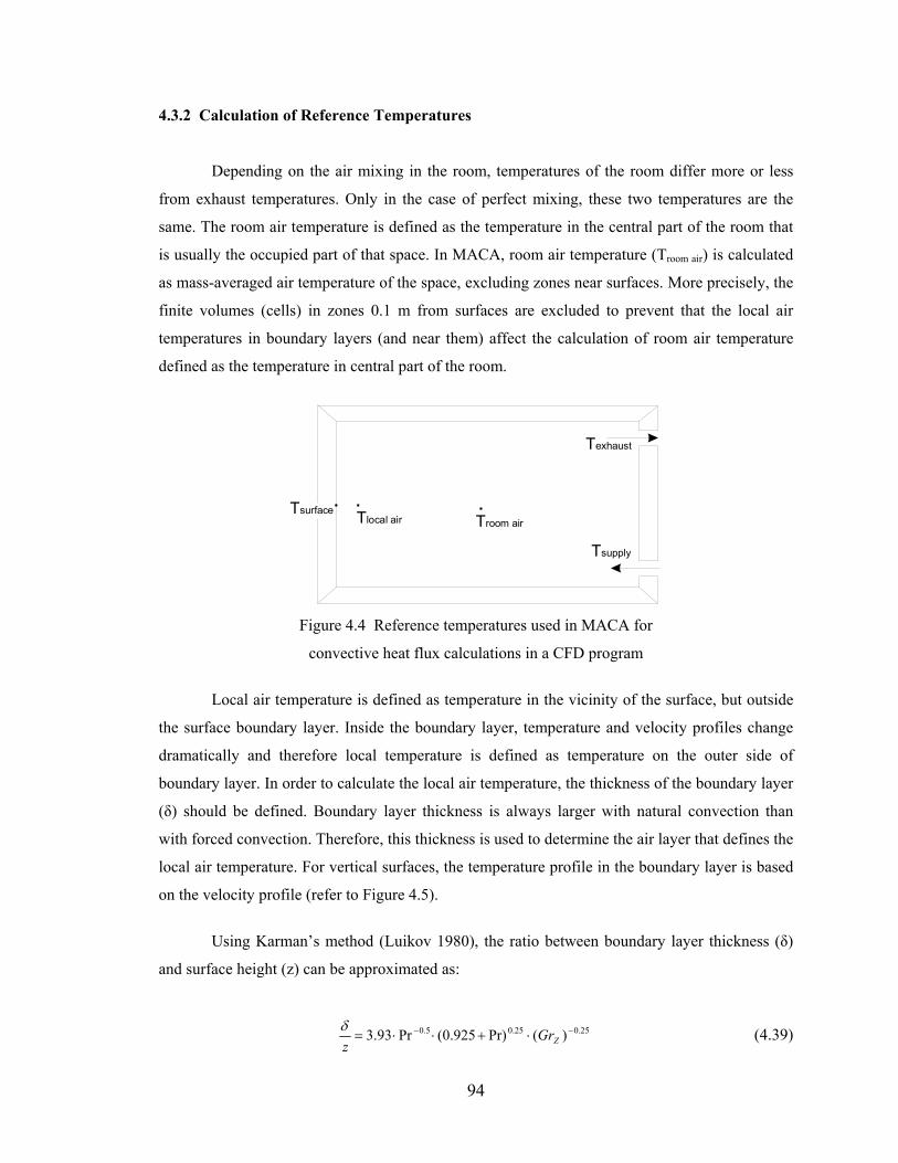
94

4.3.2 Calculation of Reference Temperatures

Depending on the air mixing in the room, temperatures of the room differ more or less

from exhaust temperatures. Only in the case of perfect mixing, these two temperatures are the

same. The room air temperature is defined as the temperature in the central part of the room that

is usually the occupied part of that space. In MACA, room air temperature (Troom air) is calculated

as mass-averaged air temperature of the space, excluding zones near surfaces. More precisely, the

finite volumes (cells) in zones 0.1 m from surfaces are excluded to prevent that the local air

temperatures in boundary layers (and near them) affect the calculation of room air temperature

defined as the temperature in central part of the room.

Tsupply

Texhaust

TsurfaceTroom airTlocal air

Figure 4.4 Reference temperatures used in MACA for

convective heat flux calculations in a CFD program

Local air temperature is defined as temperature in the vicinity of the surface, but outside

the surface boundary layer. Inside the boundary layer, temperature and velocity profiles change

dramatically and therefore local temperature is defined as temperature on the outer side of

boundary layer. In order to calculate the local air temperature, the thickness of the boundary layer

(δ) should be defined. Boundary layer thickness is always larger with natural convection than

with forced convection. Therefore, this thickness is used to determine the air layer that defines the

local air temperature. For vertical surfaces, the temperature profile in the boundary layer is based

on the velocity profile (refer to Figure 4.5).

Using Karman’s method (Luikov 1980), the ratio between boundary layer thickness (δ)

and surface height (z) can be approximated as:

25.025.05.0 )(Pr)925.0(Pr93.3 −− ⋅+⋅⋅= ZGrzδ (4.39)

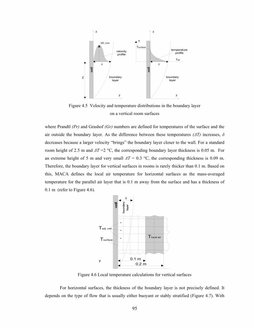
95

boundary layer

uZ_max

yw

all

z

Z

δ

velocityprofile

boundary layer

y

wal

l

z

δ

temperatureprofile

T

Tsurface

Tair

Figure 4.5 Velocity and temperature distributions in the boundary layer

on a vertical room surfaces

where Prandtl (Pr) and Grashof (Gr) numbers are defined for temperatures of the surface and the

air outside the boundary layer. As the difference between these temperatures (∆T) increases, δ

decreases because a larger velocity “brings” the boundary layer closer to the wall. For a standard

room height of 2.5 m and ∆T =2 °C, the corresponding boundary layer thickness is 0.05 m. For

an extreme height of 5 m and very small ∆T = 0.3 °C, the corresponding thickness is 0.09 m.

Therefore, the boundary layer for vertical surfaces in rooms is rarely thicker than 0.1 m. Based on

this, MACA defines the local air temperature for horizontal surfaces as the mass-averaged

temperature for the parallel air layer that is 0.1 m away from the surface and has a thickness of

0.1 m (refer to Figure 4.6).

boun

dary

la

yer

y

wal

l

δ

Tlocal air

0.1 m0.2 m

Tsurface

Tadj. cell

Figure 4.6 Local temperature calculations for vertical surfaces

For horizontal surfaces, the thickness of the boundary layer is not precisely defined. It

depends on the type of flow that is usually either buoyant or stably stratified (Figure 4.7). With

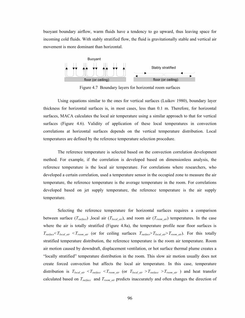
96

buoyant boundary airflow, warm fluids have a tendency to go upward, thus leaving space for

incoming cold fluids. With stably stratified flow, the fluid is gravitationally stable and vertical air

movement is more dominant than horizontal.

floor (or ceiling)floor (or ceiling) floor (or ceiling)

Buoyant

Stably stratified

Figure 4.7 Boundary layers for horizontal room surfaces

Using equations similar to the ones for vertical surfaces (Luikov 1980), boundary layer

thickness for horizontal surfaces is, in most cases, less than 0.1 m. Therefore, for horizontal

surfaces, MACA calculates the local air temperature using a similar approach to that for vertical

surfaces (Figure 4.6). Validity of application of these local temperatures in convection

correlations at horizontal surfaces depends on the vertical temperature distribution. Local

temperatures are defined by the reference temperature selection procedure.

The reference temperature is selected based on the convection correlation development

method. For example, if the correlation is developed based on dimensionless analysis, the

reference temperature is the local air temperature. For correlations where researchers, who

developed a certain correlation, used a temperature sensor in the occupied zone to measure the air

temperature, the reference temperature is the average temperature in the room. For correlations

developed based on jet supply temperature, the reference temperature is the air supply

temperature.

Selecting the reference temperature for horizontal surfaces requires a comparison

between surface (Tsurface) ,local air (Tlocal_air), and room air (Troom_air) temperatures. In the case

where the air is totally stratified (Figure 4.8a), the temperature profile near floor surfaces is

Tsurface<Tlocal_air <Troom_air (or for ceiling surfaces Tsurface>Tlocal_air>Troom_air). For this totally

stratified temperature distribution, the reference temperature is the room air temperature. Room

air motion caused by downdraft, displacement ventilation, or hot surface thermal plume creates a

“locally stratified” temperature distribution in the room. This slow air motion usually does not

create forced convection but affects the local air temperature. In this case, temperature

distribution is Tlocal_air <Tsurface <Troom_air (or Tlocal_air >Tsurface >Troom_air ) and heat transfer

calculated based on Tsurface and Troom_air predicts inaccurately and often changes the direction of

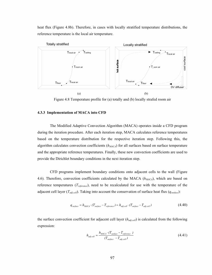
97

heat flux (Figure 4.8b). Therefore, in cases with locally stratified temperature distributions, the

reference temperature is the local air temperature.

Tceiling

Tfloor Tlocal air

Tlocal air

Troom air

Totally stratified

Tceiling

Tfloor Tlocal air

Tlocal air

Troom air

Locally stratified

hot s

urfa

ce

cool

sur

face

hot s

urfa

ceho

t sur

face

DV diffuser (a) (b)

Figure 4.8 Temperature profile for (a) totally and (b) locally strafed room air

4.3.3 Implementation of MACA into CFD

The Modified Adaptive Convection Algorithm (MACA) operates inside a CFD program

during the iteration procedure. After each iteration step, MACA calculates reference temperatures

based on the temperature distribution for the respective iteration step. Following this, the

algorithm calculates convection coefficients (hMACA) for all surfaces based on surface temperature

and the appropriate reference temperatures. Finally, these new convection coefficients are used to

provide the Dirichlet boundary conditions in the next iteration step.

CFD programs implement boundary conditions onto adjacent cells to the wall (Figure

4.6). Therefore, convection coefficients calculated by the MACA (hMACA), which are based on

reference temperatures (Treference), need to be recalculated for use with the temperature of the

adjacent cell layer (Tadj.cell). Taking into account the conservation of surface heat flux (qsurface):

)T(Th)T(Thq celladjsurfaceadj.cellreferencesurfaceMACAsurface .−⋅=−⋅= (4.40)

the surface convection coefficient for adjacent cell layer (hadj.cell) is calculated from the following

expression:

)T (T )T(Th

hcelladjsurface

reference surfaceMACAadj.cell

.−

−⋅= (4.41)

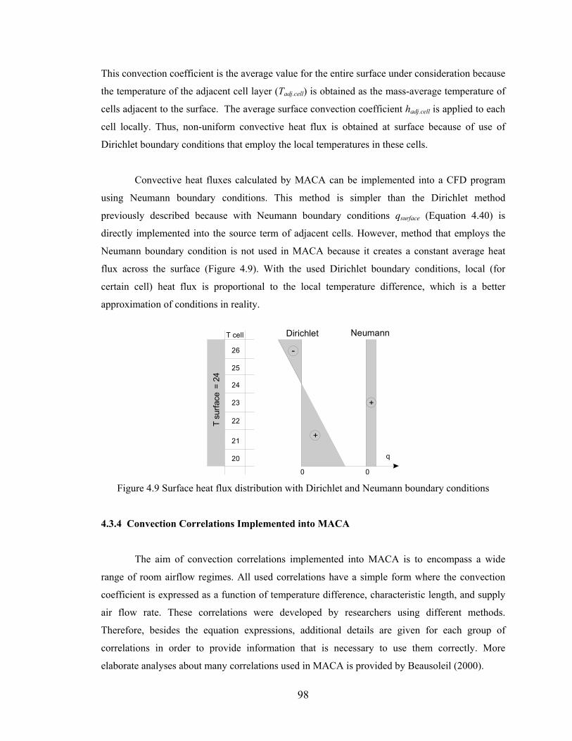
98

This convection coefficient is the average value for the entire surface under consideration because

the temperature of the adjacent cell layer (Tadj.cell) is obtained as the mass-average temperature of

cells adjacent to the surface. The average surface convection coefficient hadj.cell is applied to each

cell locally. Thus, non-uniform convective heat flux is obtained at surface because of use of

Dirichlet boundary conditions that employ the local temperatures in these cells.

Convective heat fluxes calculated by MACA can be implemented into a CFD program

using Neumann boundary conditions. This method is simpler than the Dirichlet method

previously described because with Neumann boundary conditions qsurface (Equation 4.40) is

directly implemented into the source term of adjacent cells. However, method that employs the

Neumann boundary condition is not used in MACA because it creates a constant average heat

flux across the surface (Figure 4.9). With the used Dirichlet boundary conditions, local (for

certain cell) heat flux is proportional to the local temperature difference, which is a better

approximation of conditions in reality.

T cell

20

21

22

23

24

25

0

T su

rface

= 2

4

Dirichlet Neumann

q

26 -

+

+

0 Figure 4.9 Surface heat flux distribution with Dirichlet and Neumann boundary conditions

4.3.4 Convection Correlations Implemented into MACA

The aim of convection correlations implemented into MACA is to encompass a wide

range of room airflow regimes. All used correlations have a simple form where the convection

coefficient is expressed as a function of temperature difference, characteristic length, and supply

air flow rate. These correlations were developed by researchers using different methods.

Therefore, besides the equation expressions, additional details are given for each group of

correlations in order to provide information that is necessary to use them correctly. More

elaborate analyses about many correlations used in MACA is provided by Beausoleil (2000).

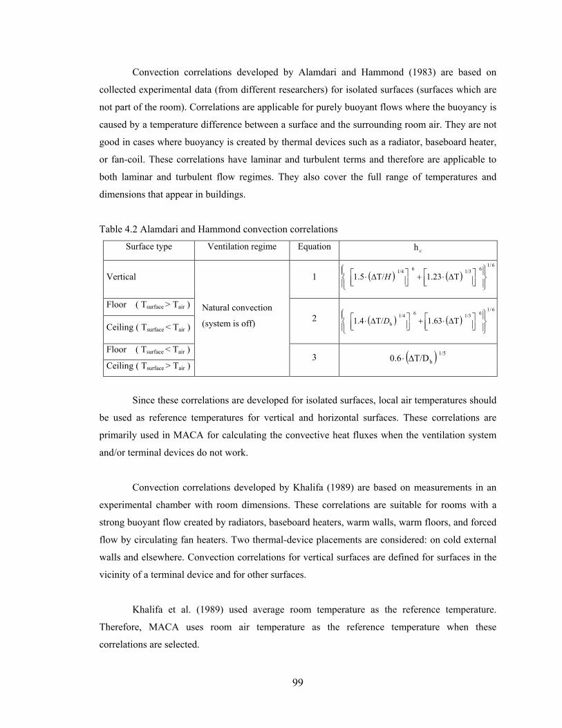
99

Convection correlations developed by Alamdari and Hammond (1983) are based on

collected experimental data (from different researchers) for isolated surfaces (surfaces which are

not part of the room). Correlations are applicable for purely buoyant flows where the buoyancy is

caused by a temperature difference between a surface and the surrounding room air. They are not

good in cases where buoyancy is created by thermal devices such as a radiator, baseboard heater,

or fan-coil. These correlations have laminar and turbulent terms and therefore are applicable to

both laminar and turbulent flow regimes. They also cover the full range of temperatures and

dimensions that appear in buildings.

Table 4.2 Alamdari and Hammond convection correlations

Surface type Ventilation regime Equation ch

Vertical 1 ( ) ( )6/1

61/361/4T23.1T/5.1

∆⋅+

∆⋅ H

Floor ( Tsurface > Tair )

Ceiling ( Tsurface < Tair ) 2 ( ) ( )

6/161/361/4

h T63.1T/4.1

∆⋅+

∆⋅ D

Floor ( Tsurface < Tair )

Ceiling ( Tsurface > Tair )

Natural convection

(system is off)

3 ( ) 1/5hT/D6.0 ∆⋅

Since these correlations are developed for isolated surfaces, local air temperatures should

be used as reference temperatures for vertical and horizontal surfaces. These correlations are

primarily used in MACA for calculating the convective heat fluxes when the ventilation system

and/or terminal devices do not work.

Convection correlations developed by Khalifa (1989) are based on measurements in an

experimental chamber with room dimensions. These correlations are suitable for rooms with a

strong buoyant flow created by radiators, baseboard heaters, warm walls, warm floors, and forced

flow by circulating fan heaters. Two thermal-device placements are considered: on cold external

walls and elsewhere. Convection correlations for vertical surfaces are defined for surfaces in the

vicinity of a terminal device and for other surfaces.

Khalifa et al. (1989) used average room temperature as the reference temperature.

Therefore, MACA uses room air temperature as the reference temperature when these

correlations are selected.

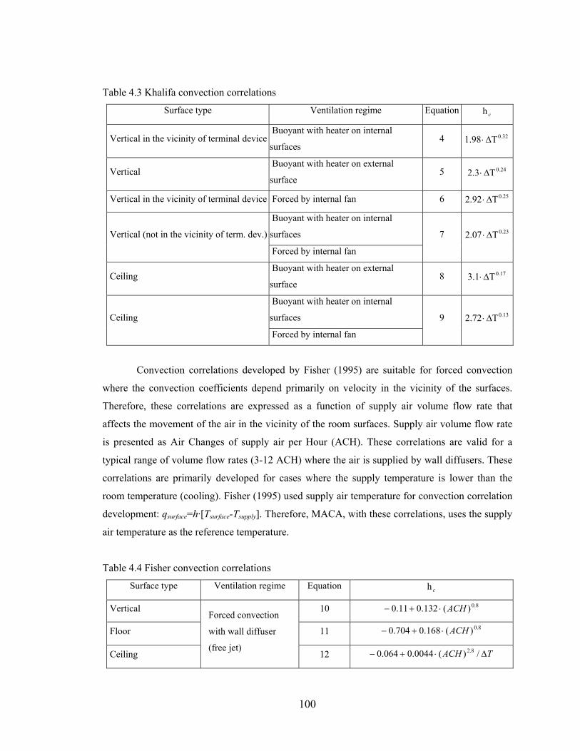
100

Table 4.3 Khalifa convection correlations

Surface type Ventilation regime Equation ch

Vertical in the vicinity of terminal device Buoyant with heater on internal

surfaces 4 0.32T1.98 ∆⋅

Vertical Buoyant with heater on external

surface 5 0.24T3.2 ∆⋅

Vertical in the vicinity of terminal device Forced by internal fan 6 0.25T92.2 ∆⋅

Buoyant with heater on internal

surfaces Vertical (not in the vicinity of term. dev.)

Forced by internal fan

7 0.23T07.2 ∆⋅

Ceiling Buoyant with heater on external

surface 8 0.17T1.3 ∆⋅

Buoyant with heater on internal

surfaces Ceiling

Forced by internal fan

9 0.13T72.2 ∆⋅

Convection correlations developed by Fisher (1995) are suitable for forced convection

where the convection coefficients depend primarily on velocity in the vicinity of the surfaces.

Therefore, these correlations are expressed as a function of supply air volume flow rate that

affects the movement of the air in the vicinity of the room surfaces. Supply air volume flow rate

is presented as Air Changes of supply air per Hour (ACH). These correlations are valid for a

typical range of volume flow rates (3-12 ACH) where the air is supplied by wall diffusers. These

correlations are primarily developed for cases where the supply temperature is lower than the

room temperature (cooling). Fisher (1995) used supply air temperature for convection correlation

development: qsurface=h·[Tsurface-Tsupply]. Therefore, MACA, with these correlations, uses the supply

air temperature as the reference temperature.

Table 4.4 Fisher convection correlations

Surface type Ventilation regime Equation ch

Vertical 10 0.8)(132.011.0 ACH⋅+−

Floor 11 0.8)(168.0704.0 ACH⋅+−

Ceiling

Forced convection

with wall diffuser

(free jet) 12 TACH ∆⋅+− /)(0044.0064.0 2.8

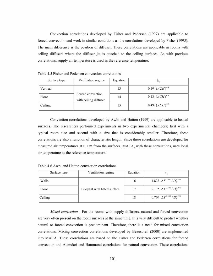
101

Convection correlations developed by Fisher and Pedersen (1997) are applicable to

forced convection and work in similar conditions as the correlations developed by Fisher (1995).

The main difference is the position of diffuser. These correlations are applicable in rooms with

ceiling diffusers where the diffuser jet is attached to the ceiling surfaces. As with previous

correlations, supply air temperature is used as the reference temperature.

Table 4.5 Fisher and Pedersen convection correlations

Surface type Ventilation regime Equation ch

Vertical 13 0.8)(19.0 ACH⋅

Floor 14 0.8)(13.0 ACH⋅

Ceiling

Forced convection

with ceiling diffuser 15 0.8)(49.0 ACH⋅

Convection correlations developed by Awbi and Hatton (1999) are applicable to heated

surfaces. The researchers performed experiments in two experimental chambers; first with a

typical room size and second with a size that is considerably smaller. Therefore, these

correlations are also a function of characteristic length. Since these correlations are developed for

measured air temperatures at 0.1 m from the surfaces, MACA, with these correlations, uses local

air temperature as the reference temperature.

Table 4.6 Awbi and Hatton convection correlations

Surface type Ventilation regime Equation ch

Walls 16 121.0293.0 /823.1 hDT∆⋅

Floor 17 076.0308.0 /175.2 hDT∆⋅

Ceiling

Buoyant with hated surface

18 601.0133.0 /704.0 hDT∆⋅

Mixed convection - For the rooms with supply diffusers, natural and forced convection

are very often present on the room surfaces at the same time. It is very difficult to predict whether

natural or forced convection is predominant. Therefore, there is a need for mixed convection

correlations. Mixing convection correlations developed by Beausoleil (2000) are implemented

into MACA. These correlations are based on the Fisher and Pedersen correlations for forced

convection and Alamdari and Hammond correlations for natural convection. These correlations

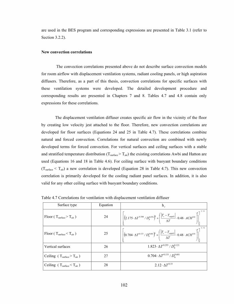
102

are used in the BES program and corresponding expressions are presented in Table 3.1 (refer to

Section 3.2.2).

New convection correlations

The convection correlations presented above do not describe surface convection models

for room airflow with displacement ventilation systems, radiant cooling panels, or high aspiration

diffusers. Therefore, as a part of this thesis, convection correlations for specific surfaces with

these ventilation systems were developed. The detailed development procedure and

corresponding results are presented in Chapters 7 and 8. Tables 4.7 and 4.8 contain only

expressions for these correlations.

The displacement ventilation diffuser creates specific air flow in the vicinity of the floor

by creating low velocity jest attached to the floor. Therefore, new convection correlations are

developed for floor surfaces (Equations 24 and 25 in Table 4.7). These correlations combine

natural and forced convection. Correlations for natural convection are combined with newly

developed terms for forced convection. For vertical surfaces and ceiling surfaces with a stable

and stratified temperature distribution (Tsurface > Tair) the existing correlations Awbi and Hatton are

used (Equations 16 and 18 in Table 4.6). For ceiling surface with buoyant boundary conditions

(Tsurface < Tair) a new correlation is developed (Equation 28 in Table 4.7). This new convection

correlation is primarily developed for the cooling radiant panel surfaces. In addition, it is also

valid for any other ceiling surface with buoyant boundary conditions.

Table 4.7 Correlations for ventilation with displacement ventilation diffuser

Surface type Equation ch

Floor ( Tsurface > Tair ) 24 ( )61

6

80607603080 4801752

/

.supplys.h

. ACH.T

TTD/T.

⋅⋅

∆

−+∆⋅

Floor ( Tsurface < Tair ) 25 ( )61

6

80660101330 4807040

/

.supplys.h

. ACH.T

TTD/T.

⋅⋅

∆

−+∆⋅

Vertical surfaces 26 121.0293.0 /823.1 hDT∆⋅

Ceiling ( Tsurface > Tair ) 27 601.0133.0 /704.0 hDT∆⋅

Ceiling ( Tsurface < Tair ) 28 33.012.2 T∆⋅

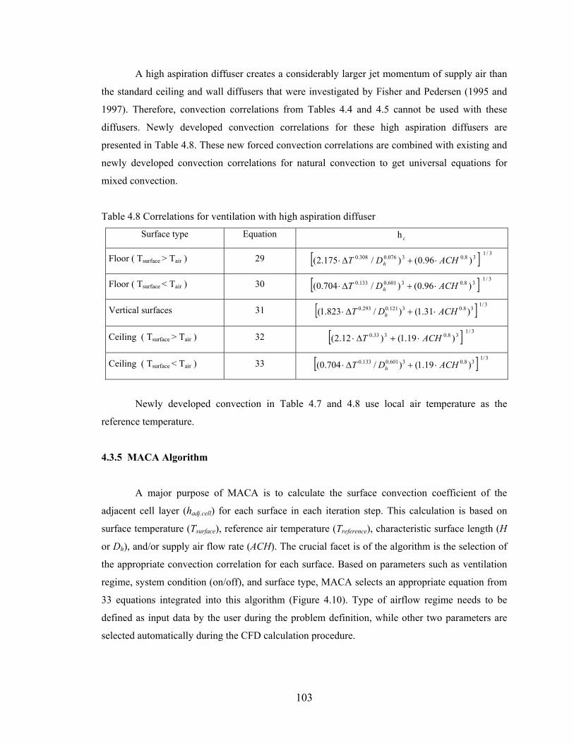
103

A high aspiration diffuser creates a considerably larger jet momentum of supply air than

the standard ceiling and wall diffusers that were investigated by Fisher and Pedersen (1995 and

1997). Therefore, convection correlations from Tables 4.4 and 4.5 cannot be used with these

diffusers. Newly developed convection correlations for these high aspiration diffusers are

presented in Table 4.8. These new forced convection correlations are combined with existing and

newly developed convection correlations for natural convection to get universal equations for

mixed convection.

Table 4.8 Correlations for ventilation with high aspiration diffuser

Surface type Equation ch

Floor ( Tsurface > Tair ) 29 [ ] 3/138.03076.0308.0 )96.0()/175.2( ACHDT h ⋅+∆⋅

Floor ( Tsurface < Tair ) 30 [ ] 3/138.03601.0133.0 )96.0()/704.0( ACHDT h ⋅+∆⋅

Vertical surfaces 31 [ ] 3/138.03121.0293.0 )31.1()/823.1( ACHDT h ⋅+∆⋅

Ceiling ( Tsurface > Tair ) 32 [ ] 3/138.0333.0 )19.1()12.2( ACHT ⋅+∆⋅

Ceiling ( Tsurface < Tair ) 33 [ ] 3/138.03601.0133.0 )19.1()/704.0( ACHDT h ⋅+∆⋅

Newly developed convection in Table 4.7 and 4.8 use local air temperature as the

reference temperature.

4.3.5 MACA Algorithm

A major purpose of MACA is to calculate the surface convection coefficient of the

adjacent cell layer (hadj.cell) for each surface in each iteration step. This calculation is based on

surface temperature (Tsurface), reference air temperature (Treference), characteristic surface length (H

or Dh), and/or supply air flow rate (ACH). The crucial facet is of the algorithm is the selection of

the appropriate convection correlation for each surface. Based on parameters such as ventilation

regime, system condition (on/off), and surface type, MACA selects an appropriate equation from

33 equations integrated into this algorithm (Figure 4.10). Type of airflow regime needs to be

defined as input data by the user during the problem definition, while other two parameters are

selected automatically during the CFD calculation procedure.

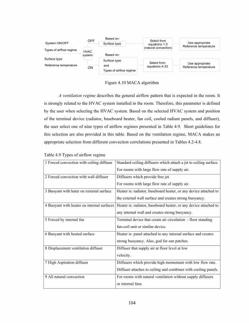
104

HVACsystem

Based on: Surface type

Based on: Surface type Types of airflow regime

OFF

ON

Select from 1-3

(natural convection) equations

Select from -33

equations 4and

Use appropriateReference temperature

Use appropriateReference temperature

Types of airflow regime

Surface type

Reference temperature

System ON/OFF

Figure 4.10 MACA algorithm

A ventilation regime describes the general airflow pattern that is expected in the room. It

is strongly related to the HVAC system installed in the room. Therefore, this parameter is defined

by the user when selecting the HVAC system. Based on the selected HVAC system and position

of the terminal device (radiator, baseboard heater, fan coil, cooled radiant panels, and diffuser),

the user select one of nine types of airflow regimes presented in Table 4.9. Short guidelines for

this selection are also provided in this table. Based on the ventilation regime, MACA makes an

appropriate selection from different convection correlations presented in Tables 4.2-4.8.

Table 4.9 Types of airflow regime

1 Forced convection with ceiling diffuser Standard ceiling diffusers which attach a jet to ceiling surface.

For rooms with large flow rate of supply air.

2 Forced convection with wall diffuser Diffusers which provide free jet.

For rooms with large flow rate of supply air.

3 Buoyant with hater on external surface Heater is: radiator, baseboard heater, or any device attached to

the external wall surface and creates strong buoyancy.

4 Buoyant with heater on internal surfaces Heater is: radiator, baseboard heater, or any device attached to

any internal wall and creates strong buoyancy.

5 Forced by internal fan Terminal device that create air circulation - floor standing

fan-coil unit or similar device.

6 Buoyant with heated surface Heater is: panel attached to any internal surface and creates

strong buoyancy. Also, god for sun patches.

8 Displacement ventilation diffuser Diffuser that supply air at floor level at low

velocity.

7 High Aspiration diffuser Diffusers which provide high momentum with low flow rate.

Diffuser attaches to ceiling and combines with cooling panels.

9 All natural convection For rooms with natural ventilation without supply diffusers

or internal fans.

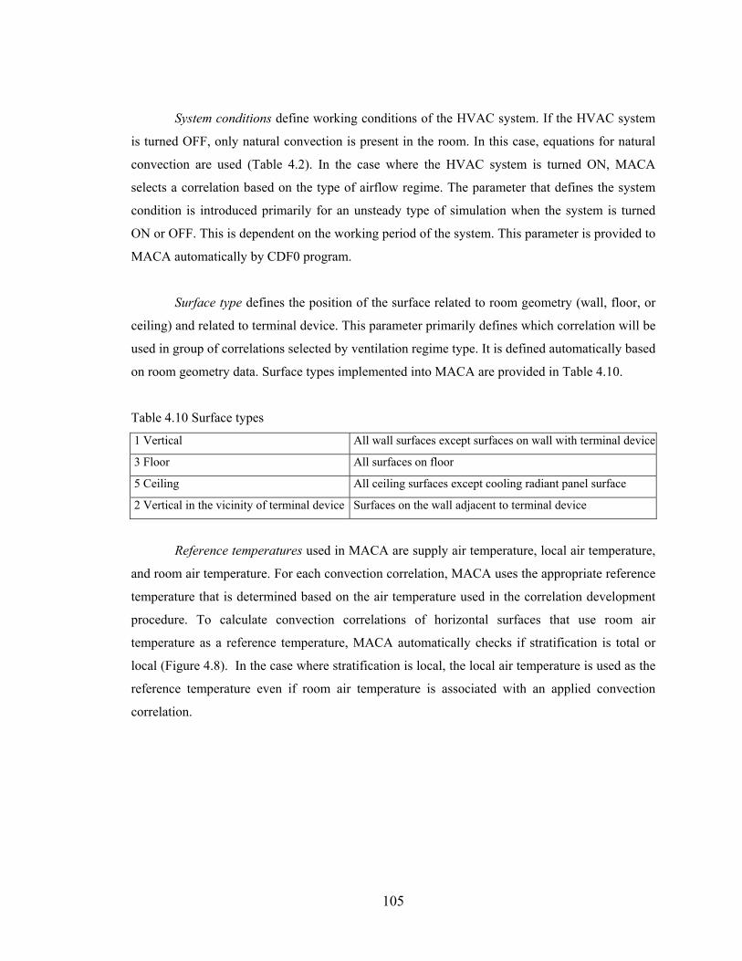
105

System conditions define working conditions of the HVAC system. If the HVAC system

is turned OFF, only natural convection is present in the room. In this case, equations for natural

convection are used (Table 4.2). In the case where the HVAC system is turned ON, MACA

selects a correlation based on the type of airflow regime. The parameter that defines the system

condition is introduced primarily for an unsteady type of simulation when the system is turned

ON or OFF. This is dependent on the working period of the system. This parameter is provided to

MACA automatically by CDF0 program.

Surface type defines the position of the surface related to room geometry (wall, floor, or

ceiling) and related to terminal device. This parameter primarily defines which correlation will be

used in group of correlations selected by ventilation regime type. It is defined automatically based

on room geometry data. Surface types implemented into MACA are provided in Table 4.10.

Table 4.10 Surface types

1 Vertical All wall surfaces except surfaces on wall with terminal device

3 Floor All surfaces on floor

5 Ceiling All ceiling surfaces except cooling radiant panel surface

2 Vertical in the vicinity of terminal device Surfaces on the wall adjacent to terminal device

Reference temperatures used in MACA are supply air temperature, local air temperature,

and room air temperature. For each convection correlation, MACA uses the appropriate reference

temperature that is determined based on the air temperature used in the correlation development

procedure. To calculate convection correlations of horizontal surfaces that use room air

temperature as a reference temperature, MACA automatically checks if stratification is total or

local (Figure 4.8). In the case where stratification is local, the local air temperature is used as the

reference temperature even if room air temperature is associated with an applied convection

correlation.

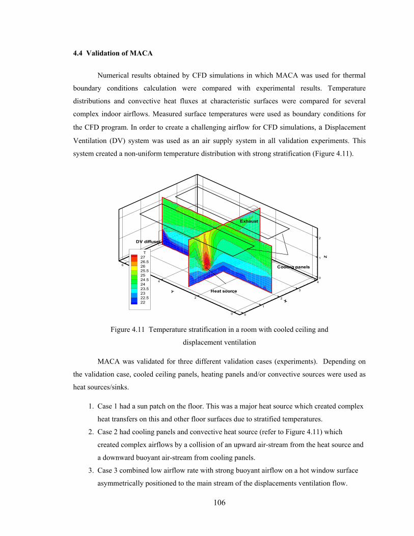
106

4.4 Validation of MACA

Numerical results obtained by CFD simulations in which MACA was used for thermal

boundary conditions calculation were compared with experimental results. Temperature

distributions and convective heat fluxes at characteristic surfaces were compared for several

complex indoor airflows. Measured surface temperatures were used as boundary conditions for

the CFD program. In order to create a challenging airflow for CFD simulations, a Displacement

Ventilation (DV) system was used as an air supply system in all validation experiments. This

system created a non-uniform temperature distribution with strong stratification (Figure 4.11).

0

1

2

Z

0

1

2

3

4

X

0

2

4

6

Y

T2726.52625.52524.52423.52322.522

DV diffuser

Exhaust

Heat source

Cooling panels

Figure 4.11 Temperature stratification in a room with cooled ceiling and

displacement ventilation MACA was validated for three different validation cases (experiments). Depending on

the validation case, cooled ceiling panels, heating panels and/or convective sources were used as

heat sources/sinks.

1. Case 1 had a sun patch on the floor. This was a major heat source which created complex

heat transfers on this and other floor surfaces due to stratified temperatures.

2. Case 2 had cooling panels and convective heat source (refer to Figure 4.11) which

created complex airflows by a collision of an upward air-stream from the heat source and

a downward buoyant air-stream from cooling panels.

3. Case 3 combined low airflow rate with strong buoyant airflow on a hot window surface

asymmetrically positioned to the main stream of the displacements ventilation flow.

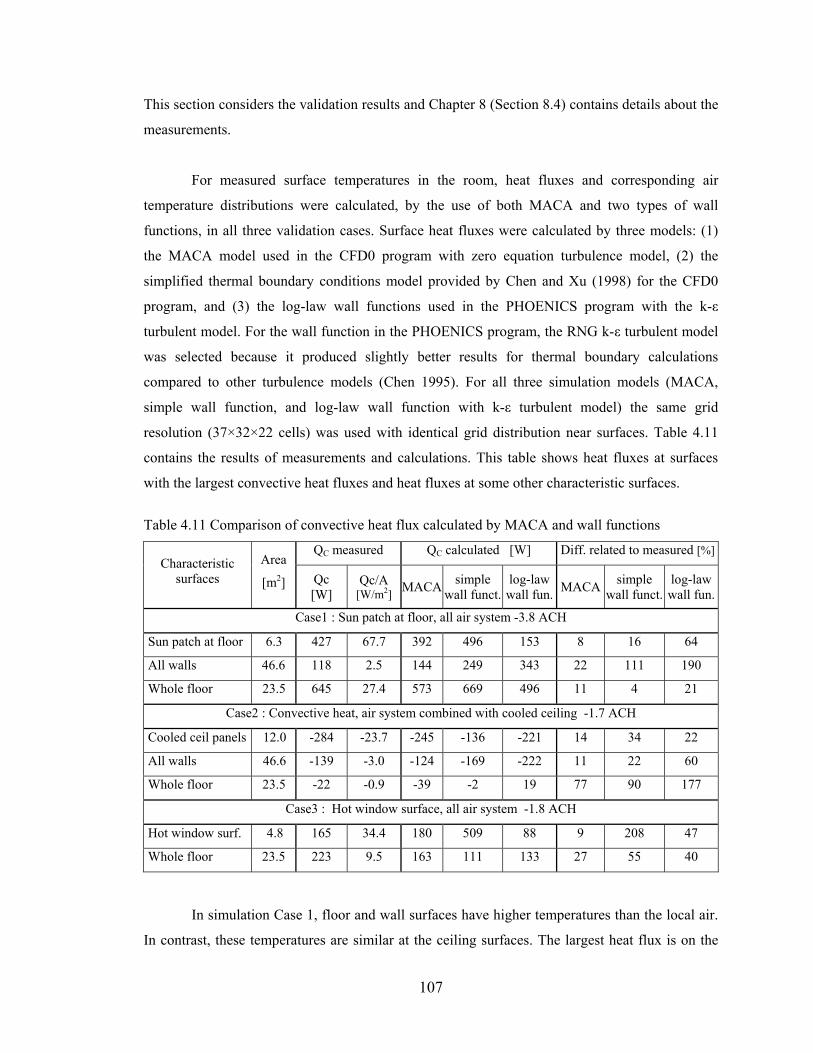
107

This section considers the validation results and Chapter 8 (Section 8.4) contains details about the

measurements.

For measured surface temperatures in the room, heat fluxes and corresponding air

temperature distributions were calculated, by the use of both MACA and two types of wall

functions, in all three validation cases. Surface heat fluxes were calculated by three models: (1)

the MACA model used in the CFD0 program with zero equation turbulence model, (2) the

simplified thermal boundary conditions model provided by Chen and Xu (1998) for the CFD0

program, and (3) the log-law wall functions used in the PHOENICS program with the k-ε

turbulent model. For the wall function in the PHOENICS program, the RNG k-ε turbulent model

was selected because it produced slightly better results for thermal boundary calculations

compared to other turbulence models (Chen 1995). For all three simulation models (MACA,

simple wall function, and log-law wall function with k-ε turbulent model) the same grid

resolution (37×32×22 cells) was used with identical grid distribution near surfaces. Table 4.11

contains the results of measurements and calculations. This table shows heat fluxes at surfaces

with the largest convective heat fluxes and heat fluxes at some other characteristic surfaces.

Table 4.11 Comparison of convective heat flux calculated by MACA and wall functions

QC measured QC calculated [W] Diff. related to measured [%]Characteristic

surfaces Area

[m2] Qc [W]

Qc/A [W/m2] MACA simple

wall funct.log-law wall fun. MACA simple

wall funct.log-law wall fun.

Case1 : Sun patch at floor, all air system -3.8 ACH

Sun patch at floor 6.3 427 67.7 392 496 153 8 16 64

All walls 46.6 118 2.5 144 249 343 22 111 190

Whole floor 23.5 645 27.4 573 669 496 11 4 21

Case2 : Convective heat, air system combined with cooled ceiling -1.7 ACH

Cooled ceil panels 12.0 -284 -23.7 -245 -136 -221 14 34 22

All walls 46.6 -139 -3.0 -124 -169 -222 11 22 60

Whole floor 23.5 -22 -0.9 -39 -2 19 77 90 177

Case3 : Hot window surface, all air system -1.8 ACH

Hot window surf. 4.8 165 34.4 180 509 88 9 208 47

Whole floor 23.5 223 9.5 163 111 133 27 55 40

In simulation Case 1, floor and wall surfaces have higher temperatures than the local air.

In contrast, these temperatures are similar at the ceiling surfaces. The largest heat flux is on the

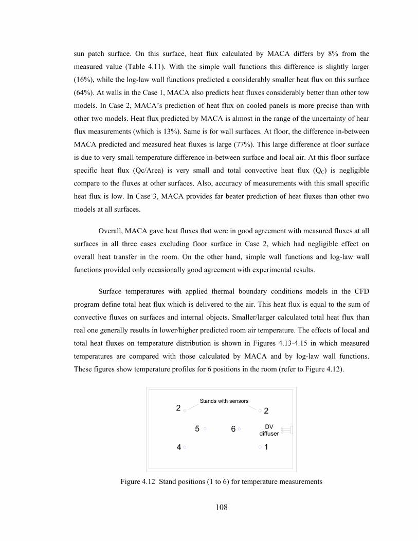
108

sun patch surface. On this surface, heat flux calculated by MACA differs by 8% from the

measured value (Table 4.11). With the simple wall functions this difference is slightly larger

(16%), while the log-law wall functions predicted a considerably smaller heat flux on this surface

(64%). At walls in the Case 1, MACA also predicts heat fluxes considerably better than other tow

models. In Case 2, MACA’s prediction of heat flux on cooled panels is more precise than with

other two models. Heat flux predicted by MACA is almost in the range of the uncertainty of hear

flux measurements (which is 13%). Same is for wall surfaces. At floor, the difference in-between

MACA predicted and measured heat fluxes is large (77%). This large difference at floor surface

is due to very small temperature difference in-between surface and local air. At this floor surface

specific heat flux (Qc/Area) is very small and total convective heat flux (QC) is negligible

compare to the fluxes at other surfaces. Also, accuracy of measurements with this small specific

heat flux is low. In Case 3, MACA provides far beater prediction of heat fluxes than other two

models at all surfaces.

Overall, MACA gave heat fluxes that were in good agreement with measured fluxes at all

surfaces in all three cases excluding floor surface in Case 2, which had negligible effect on

overall heat transfer in the room. On the other hand, simple wall functions and log-law wall

functions provided only occasionally good agreement with experimental results.

Surface temperatures with applied thermal boundary conditions models in the CFD

program define total heat flux which is delivered to the air. This heat flux is equal to the sum of

convective fluxes on surfaces and internal objects. Smaller/larger calculated total heat flux than

real one generally results in lower/higher predicted room air temperature. The effects of local and

total heat fluxes on temperature distribution is shown in Figures 4.13-4.15 in which measured

temperatures are compared with those calculated by MACA and by log-law wall functions.

These figures show temperature profiles for 6 positions in the room (refer to Figure 4.12).

Stands with sensors

1

2 2

4

5 6 DVdiffuser

Figure 4.12 Stand positions (1 to 6) for temperature measurements

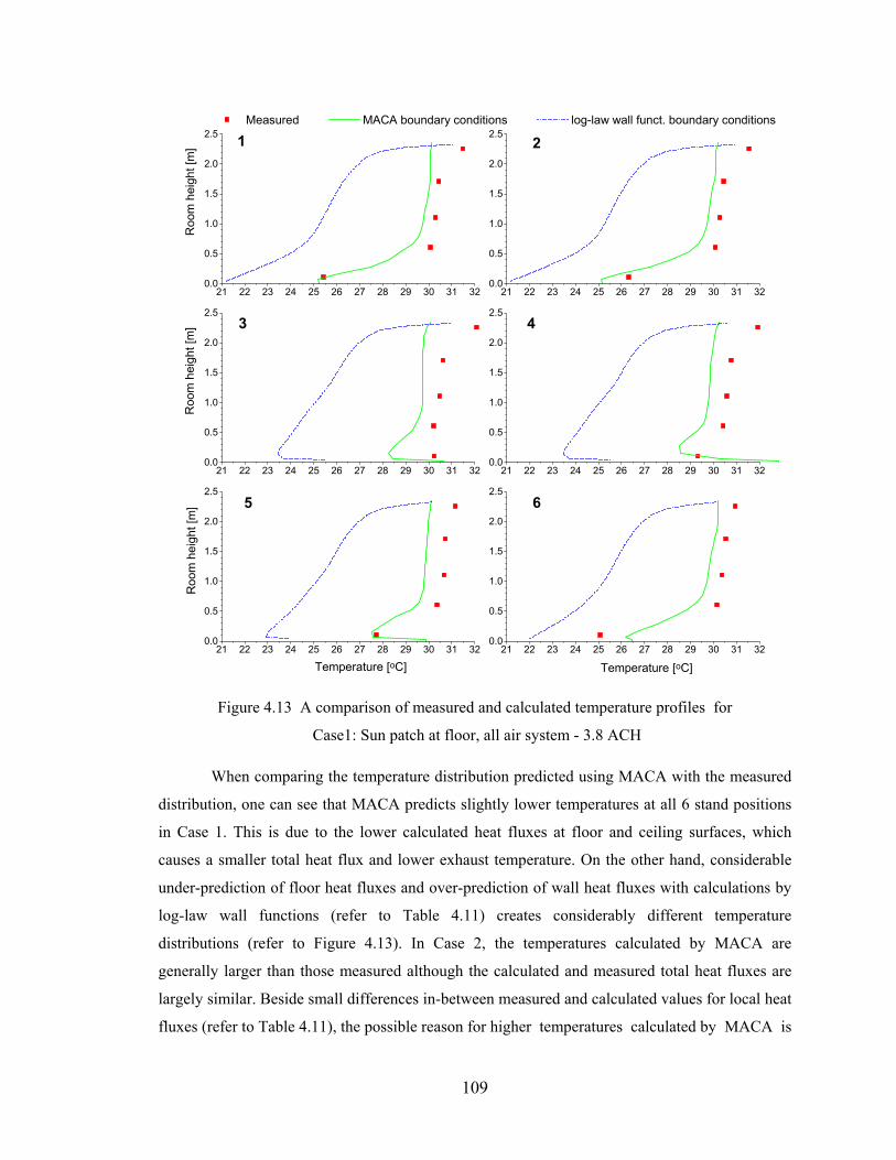
109

21 22 23 24 25 26 27 28 29 30 31 320.0

0.5

1.0

1.5

2.0

2.5 2

3 4

5 6

1

Temperature [oC]

Roo

m h

eigh

t [m

]

Temperature [oC]

Roo

m h

eigh

t [m

]R

oom

hei

ght [

m]

Measured MACA boundary conditions log-law wall funct. boundary conditions

21 22 23 24 25 26 27 28 29 30 31 320.0

0.5

1.0

1.5

2.0

2.5

21 22 23 24 25 26 27 28 29 30 31 320.0

0.5

1.0

1.5

2.0

2.5

21 22 23 24 25 26 27 28 29 30 31 320.0

0.5

1.0

1.5

2.0

2.5

21 22 23 24 25 26 27 28 29 30 31 320.0

0.5

1.0

1.5

2.0

2.5

21 22 23 24 25 26 27 28 29 30 31 320.0

0.5

1.0

1.5

2.0

2.5

Figure 4.13 A comparison of measured and calculated temperature profiles for

Case1: Sun patch at floor, all air system - 3.8 ACH When comparing the temperature distribution predicted using MACA with the measured

distribution, one can see that MACA predicts slightly lower temperatures at all 6 stand positions

in Case 1. This is due to the lower calculated heat fluxes at floor and ceiling surfaces, which

causes a smaller total heat flux and lower exhaust temperature. On the other hand, considerable

under-prediction of floor heat fluxes and over-prediction of wall heat fluxes with calculations by

log-law wall functions (refer to Table 4.11) creates considerably different temperature

distributions (refer to Figure 4.13). In Case 2, the temperatures calculated by MACA are

generally larger than those measured although the calculated and measured total heat fluxes are

largely similar. Beside small differences in-between measured and calculated values for local heat

fluxes (refer to Table 4.11), the possible reason for higher temperatures calculated by MACA is

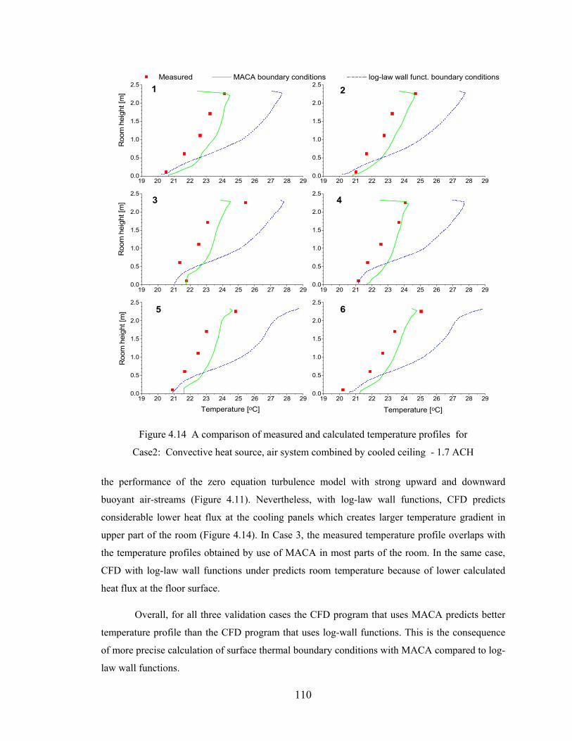
110

19 20 21 22 23 24 25 26 27 28 290.0

0.5

1.0

1.5

2.0

2.5 2

3 4

5 6

1

Temperature [oC]

Roo

m h

eigh

t [m

]

Temperature [oC]

Roo

m h

eigh

t [m

]R

oom

hei

ght [

m]

Measured MACA boundary conditions log-law wall funct. boundary conditions

19 20 21 22 23 24 25 26 27 28 290.0

0.5

1.0

1.5

2.0

2.5

19 20 21 22 23 24 25 26 27 28 290.0

0.5

1.0

1.5

2.0

2.5

19 20 21 22 23 24 25 26 27 28 290.0

0.5

1.0

1.5

2.0

2.5

19 20 21 22 23 24 25 26 27 28 290.0

0.5

1.0

1.5

2.0

2.5

19 20 21 22 23 24 25 26 27 28 290.0

0.5

1.0

1.5

2.0

2.5

Figure 4.14 A comparison of measured and calculated temperature profiles for

Case2: Convective heat source, air system combined by cooled ceiling - 1.7 ACH

the performance of the zero equation turbulence model with strong upward and downward

buoyant air-streams (Figure 4.11). Nevertheless, with log-law wall functions, CFD predicts

considerable lower heat flux at the cooling panels which creates larger temperature gradient in

upper part of the room (Figure 4.14). In Case 3, the measured temperature profile overlaps with

the temperature profiles obtained by use of MACA in most parts of the room. In the same case,

CFD with log-law wall functions under predicts room temperature because of lower calculated

heat flux at the floor surface. Overall, for all three validation cases the CFD program that uses MACA predicts better

temperature profile than the CFD program that uses log-wall functions. This is the consequence

of more precise calculation of surface thermal boundary conditions with MACA compared to log-

law wall functions.

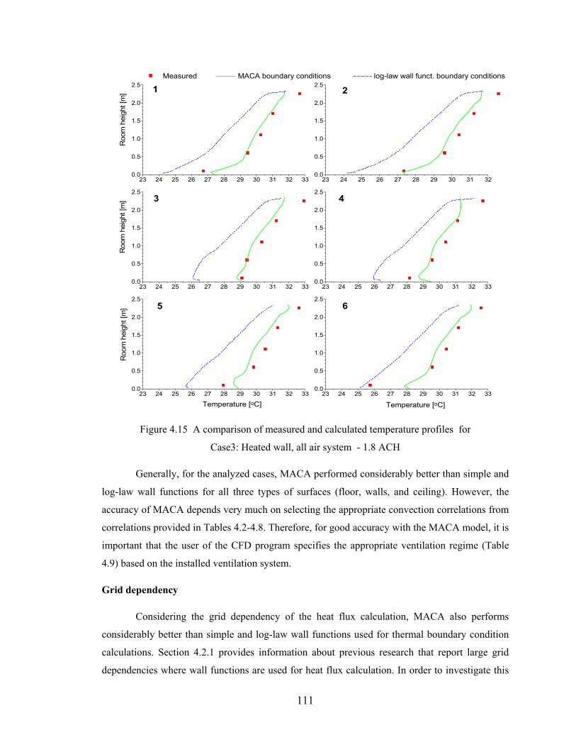
111

23 24 25 26 27 28 29 30 31 32 330.0

0.5

1.0

1.5

2.0

2.5 2

3 4

5 6

1

Temperature [oC]

Roo

m h

eigh

t [m

]

Temperature [oC]

Roo

m h

eigh

t [m

]R

oom

hei

ght [

m]

Measured MACA boundary conditions log-law wall funct. boundary conditions

23 24 25 26 27 28 29 30 31 320.0

0.5

1.0

1.5

2.0

2.5

23 24 25 26 27 28 29 30 31 32 330.0

0.5

1.0

1.5

2.0

2.5

23 24 25 26 27 28 29 30 31 32 330.0

0.5

1.0

1.5

2.0

2.5

23 24 25 26 27 28 29 30 31 32 330.0

0.5

1.0

1.5

2.0

2.5

23 24 25 26 27 28 29 30 31 32 330.0

0.5

1.0

1.5

2.0

2.5

Figure 4.15 A comparison of measured and calculated temperature profiles for

Case3: Heated wall, all air system - 1.8 ACH Generally, for the analyzed cases, MACA performed considerably better than simple and

log-law wall functions for all three types of surfaces (floor, walls, and ceiling). However, the

accuracy of MACA depends very much on selecting the appropriate convection correlations from

correlations provided in Tables 4.2-4.8. Therefore, for good accuracy with the MACA model, it is

important that the user of the CFD program specifies the appropriate ventilation regime (Table

4.9) based on the installed ventilation system. Grid dependency Considering the grid dependency of the heat flux calculation, MACA also performs

considerably better than simple and log-law wall functions used for thermal boundary condition

calculations. Section 4.2.1 provides information about previous research that report large grid

dependencies where wall functions are used for heat flux calculation. In order to investigate this

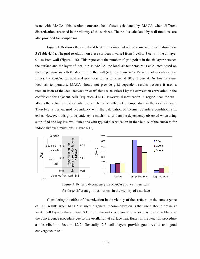
112

issue with MACA, this section compares heat fluxes calculated by MACA when different

discretizations are used in the vicinity of the surfaces. The results calculated by wall functions are

also provided for comparison. Figure 4.16 shows the calculated heat fluxes on a hot window surface in validation Case

3 (Table 4.11). The grid resolution on these surfaces is varied from 1 cell to 3 cells in the air layer

0.1 m from wall (Figure 4.16). This represents the number of grid points in the air-layer between

the surface and the layer of local air. In MACA, the local air temperature is calculated based on

the temperature in cells 0.1-0.2 m from the wall (refer to Figure 4.6). Variation of calculated heat

fluxes, by MACA, for analyzed grid variation is in range of 10% (Figure 4.16). For the same

local air temperature, MACA should not provide grid dependent results because it uses a

recalculation of the local convection coefficient as calculated by the convection correlation to the

coefficient for adjacent cells (Equation 4.41). However, discretization in region near the wall

affects the velocity field calculation, which further affects the temperature in the local air layer.

Therefore, a certain grid dependency with the calculation of thermal boundary conditions still

exists. However, this grid dependency is much smaller than the dependency observed when using

simplified and log-law wall functions with typical discretization in the vicinity of the surfaces for

indoor airflow simulations (Figure 4.16).

Wal

l

0.0

0.05

0.10

0.04 0.10

0.10

0.21

0.21

0.21

laye

r for

loca

l air

tem

pera

ture

cal

cula

tions

in M

ACA

distance from wall [m]

3 cells

2 cells

1 cell

0.02

0

100

200

300

400

500

600

700

MACA simplified b. c. log-law wall f.

1cell

2cells

3cells

q [W

/m2 ]

Figure 4.16 Grid dependency for MACA and wall functions

for three different grid resolutions in the vicinity of a surface Considering the effect of discretization in the vicinity of the surfaces on the convergence

of CFD results when MACA is used, a general recommendation is that users should define at

least 1 cell layer in the air layer 0.1m from the surfaces. Coarser meshes may create problems in

the convergence procedure due to the oscillation of surface heat fluxes in the iteration procedure

as described in Section 4.2.2. Generally, 2-3 cells layers provide good results and good

convergence rates.

113

4.5 Discussion and Summary

The previous section illustrates that MACA provides more accurate calculations of heat

fluxes on building surfaces than wall functions in the cases where the air flow type in the room is

described with convection correlations implemented in MACA. By adding more correlations for

specific air flows, the performance of this algorithm with various indoor airflow types can be

further improved.

Compared to the previous model, which uses experiment-based convection correlations

developed by Beausoleil (2000), MACA is simpler and less computationally expensive. The

previous model that uses the “Adaptive Convection Algorithm” (ACA) in combination with

“Adaptive Conflation Controller” (ACC) requires a double run of the CFD program (refer to

Section 2.3.1). With this model, adaptive convection algorithm (ACA) defines the convection

coefficients in-between two runs of CFD program. With MACA, convection coefficients are

calculated in the convergence procedure which considerably speeds up the calculation. Also, by

use of local temperatures, the performance of MACA is improved compared to ACA which use

temperatures in the adjacent (first) cells. On the other hand, the use of the Adaptive Conflation

Controller and second run of CFD in Beausoleil’s model increase the accuracy of heat flux

calculation on surfaces where experiment-based convection correlations are not suitable. These

are surfaces with local effects such as surfaces in the vicinity of the diffusers where experiment-

based convection correlations developed for average temperatures are not suitable. Generally,

MACA is faster and more flexible when it comes to the coupling with the energy simulation

program, while Beausoleil’s models (ACA and ACC) are more flexible when dealing with an

application with different airflow regimes.

114

CHAPTER 5

COUPLING OF ENERGY SIMULATION AND AIR FLOW PROGRAMS

5.1 Introduction

Pertaining to the accuracy of results obtained by the coupled program, the most important

boundary conditions are convective heat transfer rates at the enclosure surfaces which connect

modeling domains of Energy Simulation (ES) and Computational Fluid Dynamics (CFD)

programs. Other than accuracy, numerical stability and computational time are also important and

they strongly depend on the coupling method. This chapter presents specific coupling procedures

and resulting simulation accuracy. Section 5.2 describes these procedures and discusses different

coupling methods. Section 5.3 compares the results of the coupled program for four selected

coupling procedures. A comparison with experimental measurements is provided in Section 5.4.

Finally, discussion and recommendations are provided in Section 5.5.

5.2 ES and CFD Programs Coupling Methods

For the coupling of ES and CFD programs, specific procedures are required due to the

different physical models and numerical schemes of these two programs. Discontinuity of heat

transfer rates in the ES and CFD domains as well as the differences in computational time are the

main reasons to keep the existing numerical schemes of the ES and CFD programs separate.

Discontinuity of heat transfer rates in the ES and CFD domains implies that characteristic

time-scales for heat transfer are very different. This difference requires different discretizations in

time (∆τ) for unsteady-state calculations. The scale analysis of transient conductive energy flow,

provided by Bejan (1995), shows that the time needed to reach a steady state condition in a

standard building wall structure is measured in hours or days. On the other hand, the time needed

to reach a steady state air temperature distribution with transient air flow in a room (with constant

boundary conditions) is measured in minutes. This indicates that several orders of magnitude

different time steps (∆τ) are needed to simulate the transient energy flow in building structures

and transient air flow in rooms. Because of the large accumulation of thermal energy in building

115

elements (walls, floor, and ceiling), the time discretization in the coupled program is defined by a

time step that provides satisfactory accuracy for transient energy flow in the domain of the ES

program. This gives a relatively large time step (∆τES ~ hour). Putting this large ∆τES in the

general transport equation for the CFD domain (Equation 4.27), the transient term (Equation

4.28) becomes much smaller than the advection and convection terms, for all variables calculated

in the CFD domain. Therefore, in the CFD transport equation, the transient term is neglected.

This means that in coupled program, the ES program provides the solution to transient heat

transfer through building elements, while the CFD program provides the solution to the steady

state temperature and velocity distribution for the considered time step.

An approximation of the steady state CFD calculations does not affect the result of an air

flow distribution as long as ∆τ is large enough (larger than few minutes), and thus the transient

term is negligible for CFD. Unsteady CFD application of airflow in buildings are required only

when fast phenomena are considered and the required time step is small enough (less than

minute) to cause that air parameters from the previous time step influence the calculation in the

present time step. However, in most of the typical building airflow simulation cases, CFD and ES

do not require coupling with small time steps. Only different kind of emergency situations with

fast release of thermal energy, such as fire, might require unsteady CFD application, which is not

the topic of this thesis.

5.2.1 One-Directional Coupling Method

The coupling of CFD and ES programs can be one-directional or two-directional. Figure

5.1 shows the schematic of one-directional coupling. With a one-directional coupling method, the

ES program calculates room surface temperatures (Tsurfaces) and heat fluxes (Qsurfaces) based on

assumption of uniform air temperature. These data are used in the CFD program as boundary

conditions. Depending on the thermal boundary conditions model in the CFD program, surface

temperature or heat fluxes are used. The CFD program with MACA provides better accuracy of

surface heat fluxes than standard CFD with wall functions as described in the previous chapter.

Therefore, for a CFD program with MACA, surface temperature should be used. On the other

hand, heat fluxes based on ES (assuming uniform temperature) are in most of the cases more

accurate than heat fluxes calculated by CFD with log-law wall functions. Therefore, specifying

heat fluxes based on the ES program results, and this way avoiding log-law wall functions, in

many cases improves the accuracy of the CFD simulations of indoor airflow.

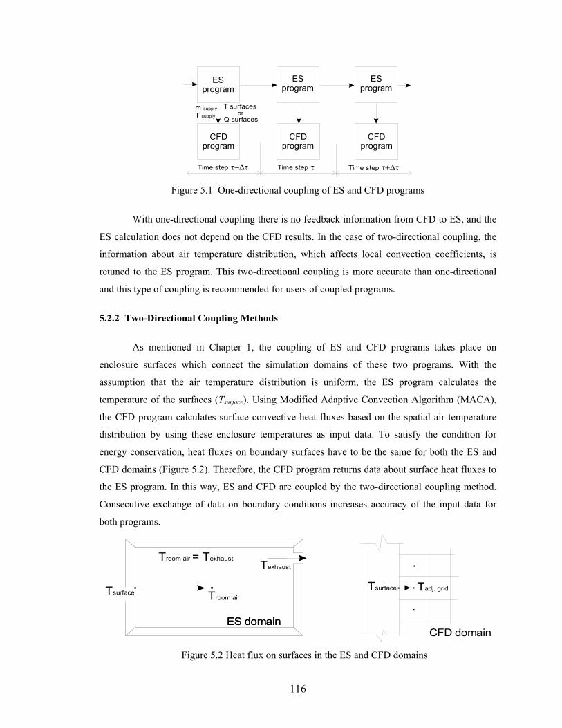
116

ESprogram

CFDprogram

ESprogram

m supply

T supply Q surfaces

Time step τTime step τ−∆τ

CFDprogram

ESprogram

CFDprogram

Time step τ+∆τ

T surfaces or

Figure 5.1 One-directional coupling of ES and CFD programs

With one-directional coupling there is no feedback information from CFD to ES, and the

ES calculation does not depend on the CFD results. In the case of two-directional coupling, the

information about air temperature distribution, which affects local convection coefficients, is

retuned to the ES program. This two-directional coupling is more accurate than one-directional

and this type of coupling is recommended for users of coupled programs.

5.2.2 Two-Directional Coupling Methods

As mentioned in Chapter 1, the coupling of ES and CFD programs takes place on

enclosure surfaces which connect the simulation domains of these two programs. With the

assumption that the air temperature distribution is uniform, the ES program calculates the

temperature of the surfaces (Tsurface). Using Modified Adaptive Convection Algorithm (MACA),

the CFD program calculates surface convective heat fluxes based on the spatial air temperature

distribution by using these enclosure temperatures as input data. To satisfy the condition for

energy conservation, heat fluxes on boundary surfaces have to be the same for both the ES and

CFD domains (Figure 5.2). Therefore, the CFD program returns data about surface heat fluxes to

the ES program. In this way, ES and CFD are coupled by the two-directional coupling method.

Consecutive exchange of data on boundary conditions increases accuracy of the input data for

both programs.

Tsurface Troom air

TexhaustTroom air = Texhaust

ES domain

Tsurface Tadj. grid

ES domainCFD domain

Figure 5.2 Heat flux on surfaces in the ES and CFD domains

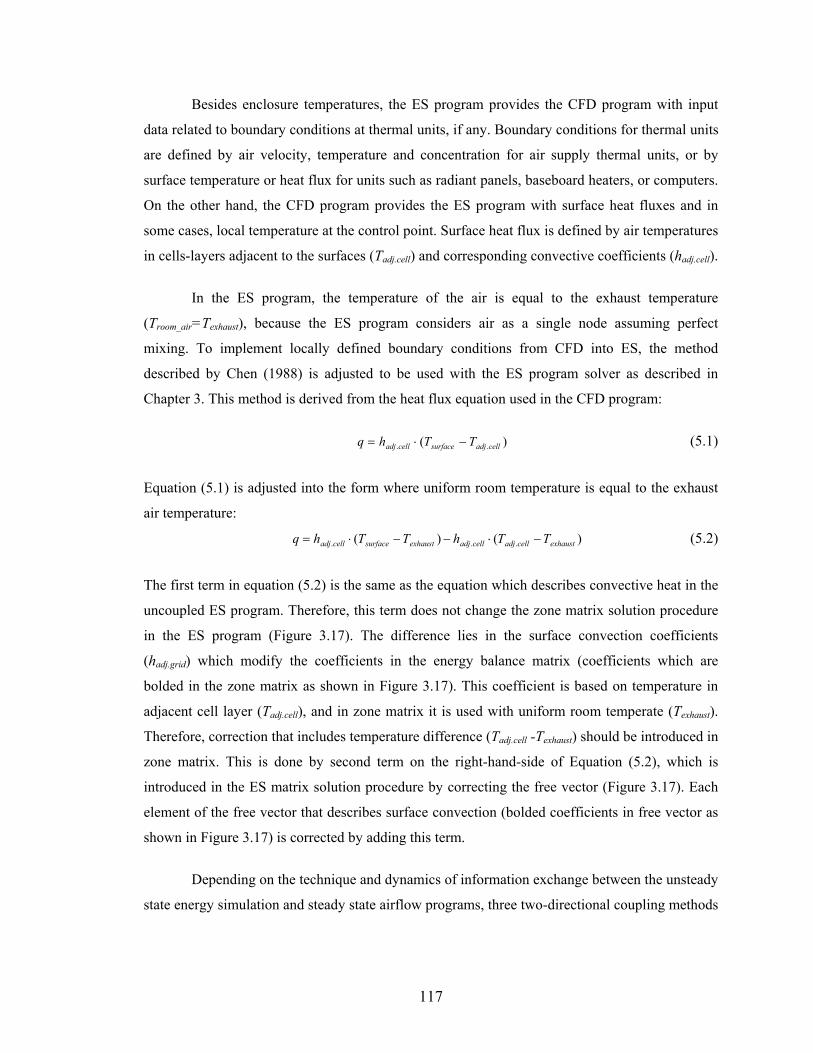
117

Besides enclosure temperatures, the ES program provides the CFD program with input

data related to boundary conditions at thermal units, if any. Boundary conditions for thermal units

are defined by air velocity, temperature and concentration for air supply thermal units, or by

surface temperature or heat flux for units such as radiant panels, baseboard heaters, or computers.

On the other hand, the CFD program provides the ES program with surface heat fluxes and in

some cases, local temperature at the control point. Surface heat flux is defined by air temperatures

in cells-layers adjacent to the surfaces (Tadj.cell) and corresponding convective coefficients (hadj.cell).

In the ES program, the temperature of the air is equal to the exhaust temperature

(Troom_air=Texhaust), because the ES program considers air as a single node assuming perfect

mixing. To implement locally defined boundary conditions from CFD into ES, the method

described by Chen (1988) is adjusted to be used with the ES program solver as described in

Chapter 3. This method is derived from the heat flux equation used in the CFD program:

)( .. celladjsurfacecelladj TThq −⋅= (5.1)

Equation (5.1) is adjusted into the form where uniform room temperature is equal to the exhaust

air temperature:

)()( ... exhaustcelladjcelladjexhaustsurfacecelladj TThTThq −⋅−−⋅= (5.2)

The first term in equation (5.2) is the same as the equation which describes convective heat in the

uncoupled ES program. Therefore, this term does not change the zone matrix solution procedure

in the ES program (Figure 3.17). The difference lies in the surface convection coefficients

(hadj.grid) which modify the coefficients in the energy balance matrix (coefficients which are

bolded in the zone matrix as shown in Figure 3.17). This coefficient is based on temperature in

adjacent cell layer (Tadj.cell), and in zone matrix it is used with uniform room temperate (Texhaust).

Therefore, correction that includes temperature difference (Tadj.cell -Texhaust) should be introduced in

zone matrix. This is done by second term on the right-hand-side of Equation (5.2), which is

introduced in the ES matrix solution procedure by correcting the free vector (Figure 3.17). Each

element of the free vector that describes surface convection (bolded coefficients in free vector as

shown in Figure 3.17) is corrected by adding this term.

Depending on the technique and dynamics of information exchange between the unsteady

state energy simulation and steady state airflow programs, three two-directional coupling methods

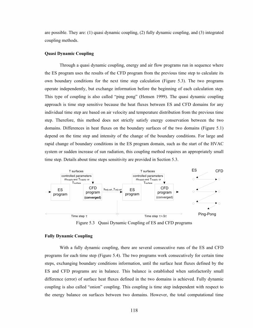
118

are possible. They are: (1) quasi dynamic coupling, (2) fully dynamic coupling, and (3) integrated

coupling methods.

Quasi Dynamic Coupling Through a quasi dynamic coupling, energy and air flow programs run in sequence where

the ES program uses the results of the CFD program from the previous time step to calculate its

own boundary conditions for the next time step calculation (Figure 5.3). The two programs

operate independently, but exchange information before the beginning of each calculation step.

This type of coupling is also called “ping pong” (Hensen 1999). The quasi dynamic coupling

approach is time step sensitive because the heat fluxes between ES and CFD domains for any

individual time step are based on air velocity and temperature distribution from the previous time

step. Therefore, this method does not strictly satisfy energy conservation between the two

domains. Differences in heat fluxes on the boundary surfaces of the two domains (Figure 5.1)

depend on the time step and intensity of the change of the boundary conditions. For large and

rapid change of boundary conditions in the ES program domain, such as the start of the HVAC

system or sudden increase of sun radiation, this coupling method requires an appropriately small

time step. Details about time steps sensitivity are provided in Section 5.3.

ESprogram

CFDprogram

(converged)(converged)

CFDprogram

(converged)

ESprogram

controlled parameters m supply

and T

Tsupply

surface or

T surfaces controlled parameters

m supply and T

Tsupply

surface or

T surfaces

hadj.cell ,Tadj.cell

Time step τ Time step τ+∆τ

ES CFD

Ping-Pong

Figure 5.3 Quasi Dynamic Coupling of ES and CFD programs

Fully Dynamic Coupling With a fully dynamic coupling, there are several consecutive runs of the ES and CFD

programs for each time step (Figure 5.4). The two programs work consecutively for certain time

steps, exchanging boundary conditions information, until the surface heat fluxes defined by the

ES and CFD programs are in balance. This balance is established when satisfactorily small

difference (error) of surface heat fluxes defined in the two domains is achieved. Fully dynamic

coupling is also called “onion” coupling. This coupling is time step independent with respect to

the energy balance on surfaces between two domains. However, the total computational time

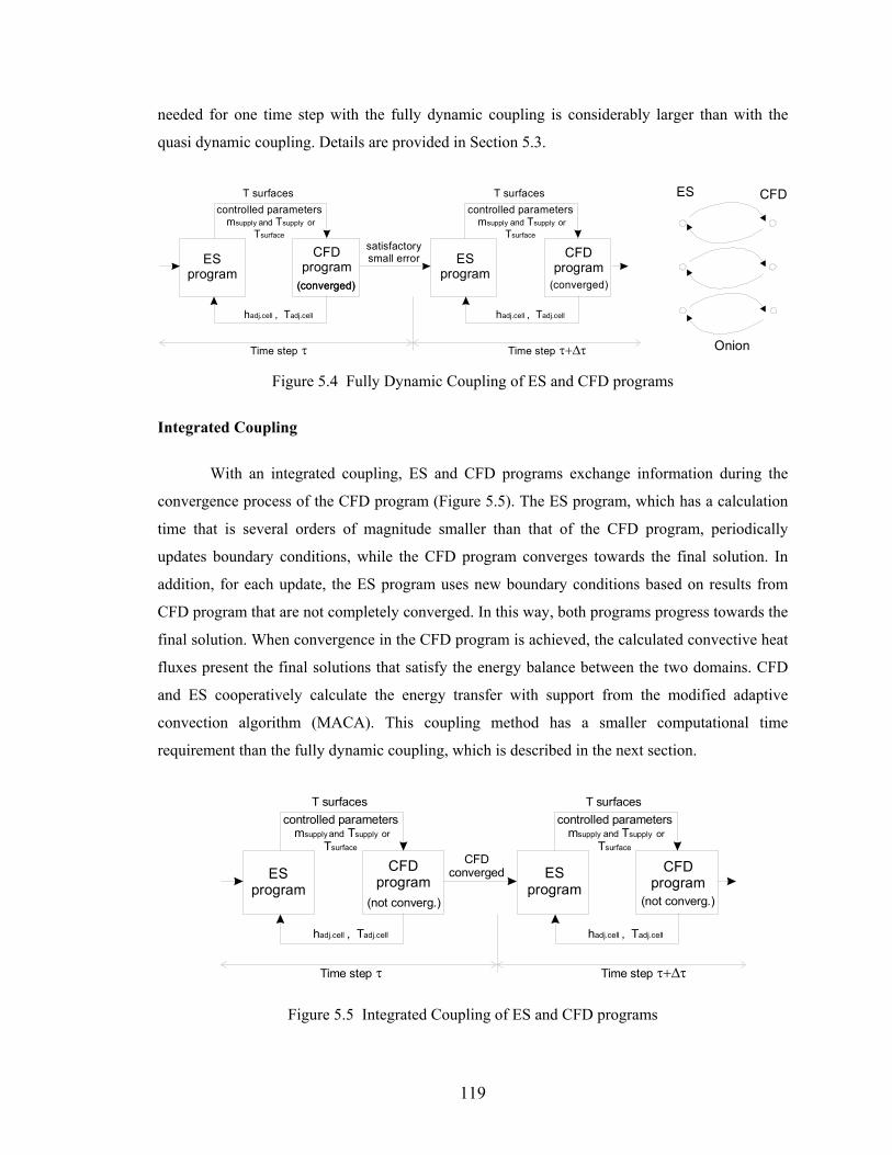
119

needed for one time step with the fully dynamic coupling is considerably larger than with the

quasi dynamic coupling. Details are provided in Section 5.3.

ESprogram

CFDprogram

(converged)(converged)

CFDprogram

(converged)

ESprogram

controlled parameters m supply and T

Tsupply

surface or

T surfaces controlled parameters

m supply and T

Tsupply

surface or

T surfaces

satisfactorysmall error

Time step τ Time step τ+∆τ

hadj.cell , Tadj.cell hadj.cell , Tadj.cell

ES CFD

Onion

Figure 5.4 Fully Dynamic Coupling of ES and CFD programs

Integrated Coupling

With an integrated coupling, ES and CFD programs exchange information during the

convergence process of the CFD program (Figure 5.5). The ES program, which has a calculation

time that is several orders of magnitude smaller than that of the CFD program, periodically

updates boundary conditions, while the CFD program converges towards the final solution. In

addition, for each update, the ES program uses new boundary conditions based on results from

CFD program that are not completely converged. In this way, both programs progress towards the

final solution. When convergence in the CFD program is achieved, the calculated convective heat

fluxes present the final solutions that satisfy the energy balance between the two domains. CFD

and ES cooperatively calculate the energy transfer with support from the modified adaptive

convection algorithm (MACA). This coupling method has a smaller computational time

requirement than the fully dynamic coupling, which is described in the next section.

ESprogram

CFDprogram

(not converg.)

CFDprogram

(not converg.)

ESprogram

controlled parameters m supply

and T

Tsupply

surface or

T surfaces controlled parameters

m supply and T

Tsupply

surface or

T surfaces

CFDconverged

Time step τ Time step τ+∆τ

hadj.cell , Tadj.cell hadj.cell , Tadj.cell

Figure 5.5 Integrated Coupling of ES and CFD programs

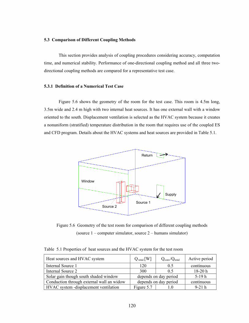
120

5.3 Comparison of Different Coupling Methods

This section provides analysis of coupling procedures considering accuracy, computation

time, and numerical stability. Performance of one-directional coupling method and all three two-

directional coupling methods are compared for a representative test case.

5.3.1 Definition of a Numerical Test Case

Figure 5.6 shows the geometry of the room for the test case. This room is 4.5m long,

3.5m wide and 2.4 m high with two internal heat sources. It has one external wall with a window

oriented to the south. Displacement ventilation is selected as the HVAC system because it creates

a nonuniform (stratified) temperature distribution in the room that requires use of the coupled ES

and CFD program. Details about the HVAC systems and heat sources are provided in Table 5.1.

Window

Source 1Source 2

Return

Supply

Figure 5.6 Geometry of the test room for comparison of different coupling methods

(source 1 – computer simulator, source 2 – humans simulator)

Table 5.1 Properties of heat sources and the HVAC system for the test room

Heat sources and HVAC system Q total [W] Qconv/Qtotal Active period Internal Source 1 120 0.5 continuous Internal Source 2 300 0.5 18-20 h Solar gain though south shaded window depends on day period 5-19 h Conduction through external wall an widow depends on day period continuous HVAC system -displacement ventilation Figure 5.7 1.0 9-21 h

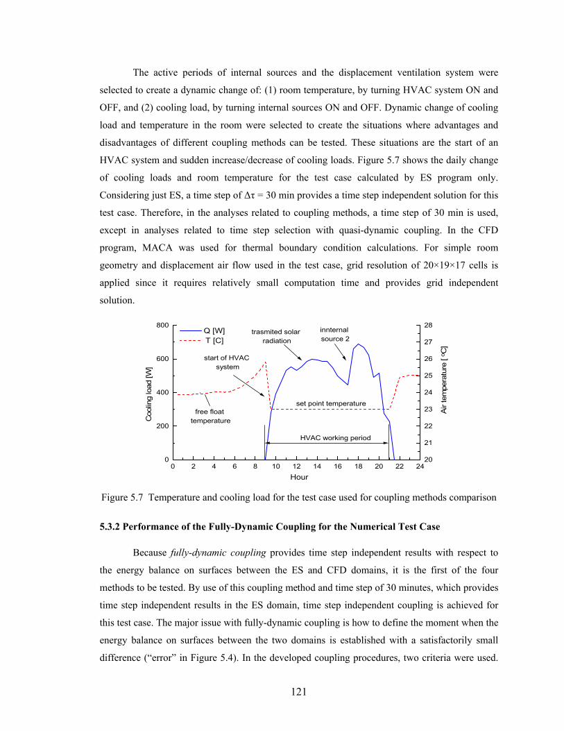
121

The active periods of internal sources and the displacement ventilation system were

selected to create a dynamic change of: (1) room temperature, by turning HVAC system ON and

OFF, and (2) cooling load, by turning internal sources ON and OFF. Dynamic change of cooling

load and temperature in the room were selected to create the situations where advantages and

disadvantages of different coupling methods can be tested. These situations are the start of an

HVAC system and sudden increase/decrease of cooling loads. Figure 5.7 shows the daily change

of cooling loads and room temperature for the test case calculated by ES program only.

Considering just ES, a time step of ∆τ = 30 min provides a time step independent solution for this

test case. Therefore, in the analyses related to coupling methods, a time step of 30 min is used,

except in analyses related to time step selection with quasi-dynamic coupling. In the CFD

program, MACA was used for thermal boundary condition calculations. For simple room

geometry and displacement air flow used in the test case, grid resolution of 20×19×17 cells is

applied since it requires relatively small computation time and provides grid independent

solution.

0 2 4 6 8 10 12 14 16 18 20 22 240

200

400

600

800

free float temperature

HVAC working period

innternal source 2

trasmited solar radiation

start of HVAC system

set point temperature

Air

tem

pera

ture

[ o C

]

Q [W]

Coo

ling

load

[W]

Hour

20

21

22

23

24

25

26

27

28

T [C]

Figure 5.7 Temperature and cooling load for the test case used for coupling methods comparison

5.3.2 Performance of the Fully-Dynamic Coupling for the Numerical Test Case Because fully-dynamic coupling provides time step independent results with respect to

the energy balance on surfaces between the ES and CFD domains, it is the first of the four

methods to be tested. By use of this coupling method and time step of 30 minutes, which provides

time step independent results in the ES domain, time step independent coupling is achieved for

this test case. The major issue with fully-dynamic coupling is how to define the moment when the

energy balance on surfaces between the two domains is established with a satisfactorily small

difference (“error” in Figure 5.4). In the developed coupling procedures, two criteria were used.

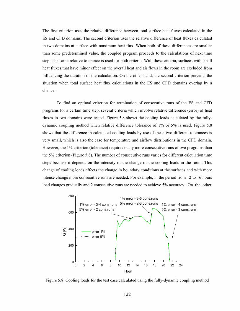
122

The first criterion uses the relative difference between total surface heat fluxes calculated in the

ES and CFD domains. The second criterion uses the relative difference of heat fluxes calculated

in two domains at surface with maximum heat flux. When both of these differences are smaller

than some predetermined value, the coupled program proceeds to the calculations of next time

step. The same relative tolerance is used for both criteria. With these criteria, surfaces with small

heat fluxes that have minor effect on the overall heat and air flows in the room are excluded from

influencing the duration of the calculation. On the other hand, the second criterion prevents the

situation when total surface heat flux calculations in the ES and CFD domains overlap by a

chance.

To find an optimal criterion for termination of consecutive runs of the ES and CFD

programs for a certain time step, several criteria which involve relative difference (error) of heat

fluxes in two domains were tested. Figure 5.8 shows the cooling loads calculated by the fully-

dynamic coupling method when relative difference tolerance of 1% or 5% is used. Figure 5.8

shows that the difference in calculated cooling loads by use of these two different tolerances is

very small, which is also the case for temperature and airflow distributions in the CFD domain.

However, the 1% criterion (tolerance) requires many more consecutive runs of two programs than

the 5% criterion (Figure 5.8). The number of consecutive runs varies for different calculation time

steps because it depends on the intensity of the change of the cooling loads in the room. This

change of cooling loads affects the change in boundary conditions at the surfaces and with more

intense change more consecutive runs are needed. For example, in the period from 12 to 16 hours

load changes gradually and 2 consecutive runs are needed to achieve 5% accuracy. On the other

0 2 4 6 8 10 12 14 16 18 20 22 240

200

400

600

8001% error - 3-5 cons.runs5% error - 2-3 cons.runs 1% error - 4 cons.runs

5% error - 3 cons.runs1% error - 3-4 cons.runs5% error - 2 cons.runs

error 1% error 5%Q

[W]

Hour Figure 5.8 Cooling loads for the test case calculated using the fully-dynamic coupling method

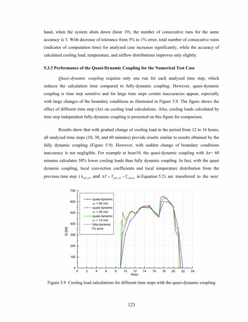
123

hand, when the system shuts down (hour 19), the number of consecutive runs for the same

accuracy is 3. With decrease of tolerance from 5% to 1% error, total number of consecutive ruins

(indicator of computation time) for analyzed case increases significantly, while the accuracy of

calculated cooling load, temperature, and airflow distributions improves only slightly.

5.3.3 Performance of the Quasi-Dynamic Coupling for the Numerical Test Case Quasi-dynamic coupling requires only one run for each analyzed time step, which

reduces the calculation time compared to fully-dynamic coupling. However, quasi-dynamic

coupling is time step sensitive and for large time steps certain inaccuracies appear, especially

with large changes of the boundary conditions as illustrated in Figure 5.9. The figure shows the

effect of different time step (∆τ) on cooling load calculations. Also, cooling loads calculated by

time step independent fully-dynamic coupling is presented on this figure for comparison.

Results show that with gradual change of cooling load in the period from 12 to 16 hours,

all analyzed time steps (10, 30, and 60 minutes) provide results similar to results obtained by the

fully dynamic coupling (Figure 5.9). However, with sudden change of boundary conditions

inaccuracy is not negligible. For example at hour10, the quasi-dynamic coupling with ∆τ= 60

minutes calculates 30% lower cooling loads than fully dynamic coupling. In fact, with the quasi

dynamic coupling, local convection coefficients and local temperature distribution from the

previous time step ( celladjh . and exhaustcelladj TTT −=∆ . in Equation 5.2) are transferred to the next

0 2 4 6 8 10 12 14 16 18 20 22 240

100

200

300

400

500

600

700

quasi-dynamic ∆τ = 60 min

quasi-dynamic ∆τ = 30 min

quasi-dynamic ∆τ = 10 min

fully-dynamic 1% error

Q [W

]

Hour Figure 5.9 Cooling load calculations for different time steps with the quasi-dynamic coupling

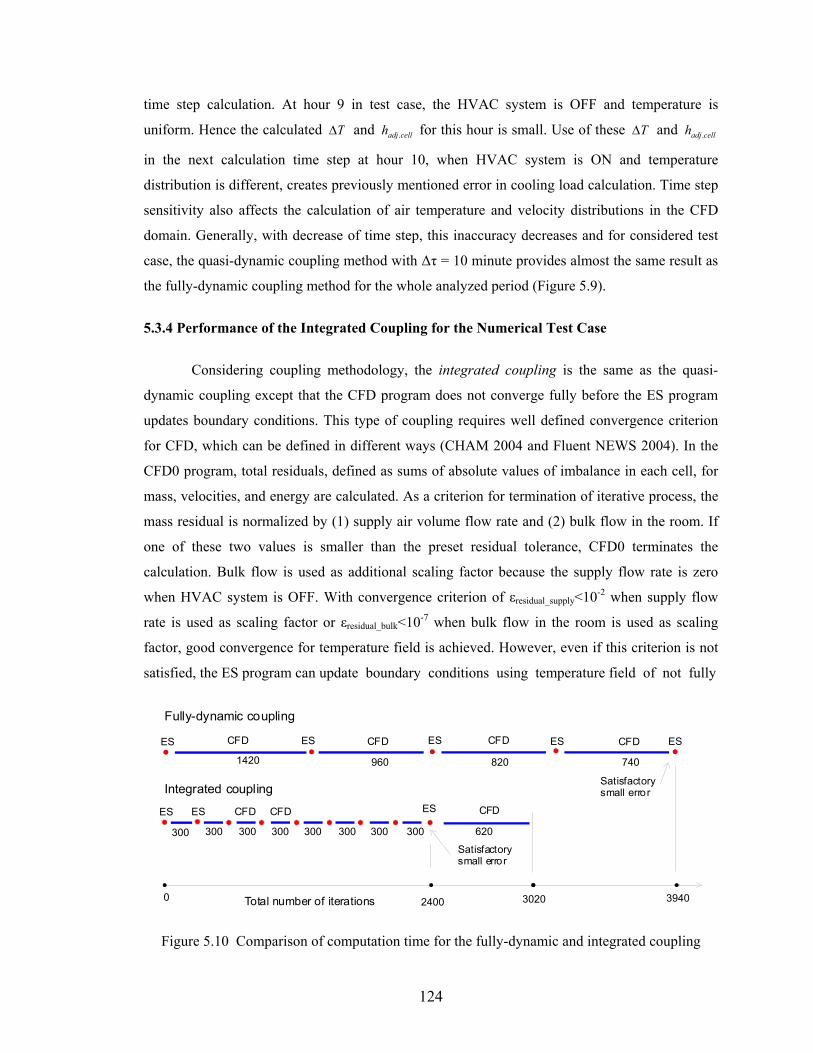
124

time step calculation. At hour 9 in test case, the HVAC system is OFF and temperature is

uniform. Hence the calculated T∆ and celladjh . for this hour is small. Use of these T∆ and celladjh .

in the next calculation time step at hour 10, when HVAC system is ON and temperature

distribution is different, creates previously mentioned error in cooling load calculation. Time step

sensitivity also affects the calculation of air temperature and velocity distributions in the CFD

domain. Generally, with decrease of time step, this inaccuracy decreases and for considered test

case, the quasi-dynamic coupling method with ∆τ = 10 minute provides almost the same result as

the fully-dynamic coupling method for the whole analyzed period (Figure 5.9).

5.3.4 Performance of the Integrated Coupling for the Numerical Test Case

Considering coupling methodology, the integrated coupling is the same as the quasi-

dynamic coupling except that the CFD program does not converge fully before the ES program

updates boundary conditions. This type of coupling requires well defined convergence criterion

for CFD, which can be defined in different ways (CHAM 2004 and Fluent NEWS 2004). In the

CFD0 program, total residuals, defined as sums of absolute values of imbalance in each cell, for

mass, velocities, and energy are calculated. As a criterion for termination of iterative process, the

mass residual is normalized by (1) supply air volume flow rate and (2) bulk flow in the room. If

one of these two values is smaller than the preset residual tolerance, CFD0 terminates the

calculation. Bulk flow is used as additional scaling factor because the supply flow rate is zero

when HVAC system is OFF. With convergence criterion of εresidual_supply<10-2 when supply flow

rate is used as scaling factor or εresidual_bulk<10-7 when bulk flow in the room is used as scaling

factor, good convergence for temperature field is achieved. However, even if this criterion is not

satisfied, the ES program can update boundary conditions using temperature field of not fully

ES CFD ES CFD CFDES ES CFD

ES CFDES CFD ES

ES

CFD

300

1420 960 820

620300 300300 300 300 300300

740

39400

Integrated coupling

Fully-dynamic coupling

Satisfactory small error

Satisfactory small error

Total number of iterations 30202400

Figure 5.10 Comparison of computation time for the fully-dynamic and integrated coupling

125

converged CFD result, where convergence is defined by εresidual_supply and εresidual_bulk. For successful

update of boundary conditions, CFD needs to converge only to a certain level. Hence, with fewer

number of iteration than needed for the full convergence, satisfactory accurate temperature

distribution can be obtained. For example, in the moment after a shutdown of HVAC system in

the test case (hour 21 in Figure 5.8), temperature field is defined to the level needed for

successful update of boundary conditions after several hundred iterations, while much more

iterations are needed to achieve the full convergence. This is illustrated in Figure 5.10.

With the fully-dynamic coupling, 4 consecutive run of the ES and CFD programs are

needed (with the total iteration number of 3940) to achieve satisfactory small error of 1% (Figure

5.10). For the same case with the integrated coupling and the same error tolerance of 1%, the

same surface heat fluxes as with the fully-dynamic coupling are obtained after 8 consecutive run

of CFD and ES program. Total number of CFD iterations that is needed to reach this result is

2400 and it is considerably smaller than with the fully-dynamic coupling. To achieve the fully

converged airflow result with the integrated coupling, an additional run of the CFD program is

needed (Figure 5.10). This additional CFD run increases the total number of iterations to 3020,

which is still considerably less than with the fully dynamic coupling.

In some simulations, the integrated coupling may create divergence of results calculated

by the coupled program. Sometimes, not fully converged CFD results that are processed by the

ES program may create unrealistic boundary conditions for the ES domain and lead to

divergence. This may happen after the first consecutive run of the programs for certain

calculation time step when the initial values for temperature field are far from the converged

result values. To avoid this, the number of CFD iterations in the first consecutive run should be

carefully selected.

5.3.5 Performance of the One-Directional Coupling for the Numerical Test Case

One-directional coupling is the simplest method that calculates up to 30% different

cooling loads than the fully dynamic coupling for the considered test case (Figures 5.7 and 5.8).

Considering temperature distributions calculated by the CFD program that uses MACA, the

temperature calculated by one-directional coupling is by 0.5°C to 1°C off when compared to

temperatures calculated by the fully dynamic coupling. The reason for this is a different surface

temperature distribution obtained by the two way coupling. In general, the one-directional

coupling is suitable for manual coupling of any ES and CFD program.

126

5.4 Summary

This section defined four ES and CFD coupling methodologies and analyzed

performance of different coupling techniques. All three two-directional coupling methods can

provide the same result. The quasi-dynamic coupling method is suitable for simulations with

gradual change of cooling loads or in simulations that require small time steps measured in

minutes such as analyses that incorporate control system models. Fully-dynamic coupling

provides time step independent solution because of default energy balance on surfaces between

the ES and CFD calculation domains. This method has the disadvantage of being computationally

expensive since it requires several consecutive runs of the ES and CFD programs. The number of

consecutive runs depends on the criterion for advancing into the next time step. An analysis

showed that a criterion of 5% heat flux difference provides good accuracy and relatively small

computation time. The integrated coupling also satisfies the energy balance on surfaces and needs

a much smaller computational time than the fully dynamic coupling. However, with this type of

coupling, the period for boundary condition updates should be carefully selected.

127

CHAPTER 6

ORGANIZATION AND GRAPHICAL USER INTERFACE OF COUPLED PROGRAM

6.1 Introduction

In the coupling of Energy Simulation (ES) and Computational Fluid Dynamics (CFD)

programs, as presented in Chapters 3, 4, and 5, a specific organization of data flow between these

two programs is needed. Both programs require a large amount of input data organized in formats

readable by these programs. In addition, output results represent a large amount of data that need

to be organized in easily understandable ways such as charts and graphics. Therefore, during the

development of a coupled program, considerable effort was made to organize these data. As a

result, a new Graphical User Interfaces (GUI) for (1) input data organization and (2) result

presentation were developed.

In the following sections, basic data about the source code of Building Energy Simulation

(BES) program and CFD program (CDF0) are presented followed by details about the structure of

the coupled program (Section 6.2). Newly developed GUI for input data is presented in Section

6.3, while the GUI for output result presentation is presented in Section 6.4. At the end of this

Chapter (Section 6.4), a short summary is provided.

6.2 Data Flow in the Coupled ES and CFD Program

Coupling models implemented into BES and CFD0 programs were selected and

developed to provide optimal accuracy for energy and airflow simulations in buildings.

Organizing these two programs into coupled program provides flexibility in addition to accuracy.

A data flow between the two programs is organized to enable different types of coupling, as

described in Chapter 5, without changing the programs’ solver procedures, as described in

Chapters 3 and 4. The data-flow procedures exchange information between two programs, which

have their source codes written in different programming languages.

The CFD0 source code is written in FORTRAN programming language. As mentioned in

Chapter 4, this code was initially developed at MIT (Srebric et al. 2000). As part of this thesis, the

CFD0 program was further developed by adding functions to calculate thermal boundary

conditions by convection correlations based on experimental measurements (Section 4.3). Input

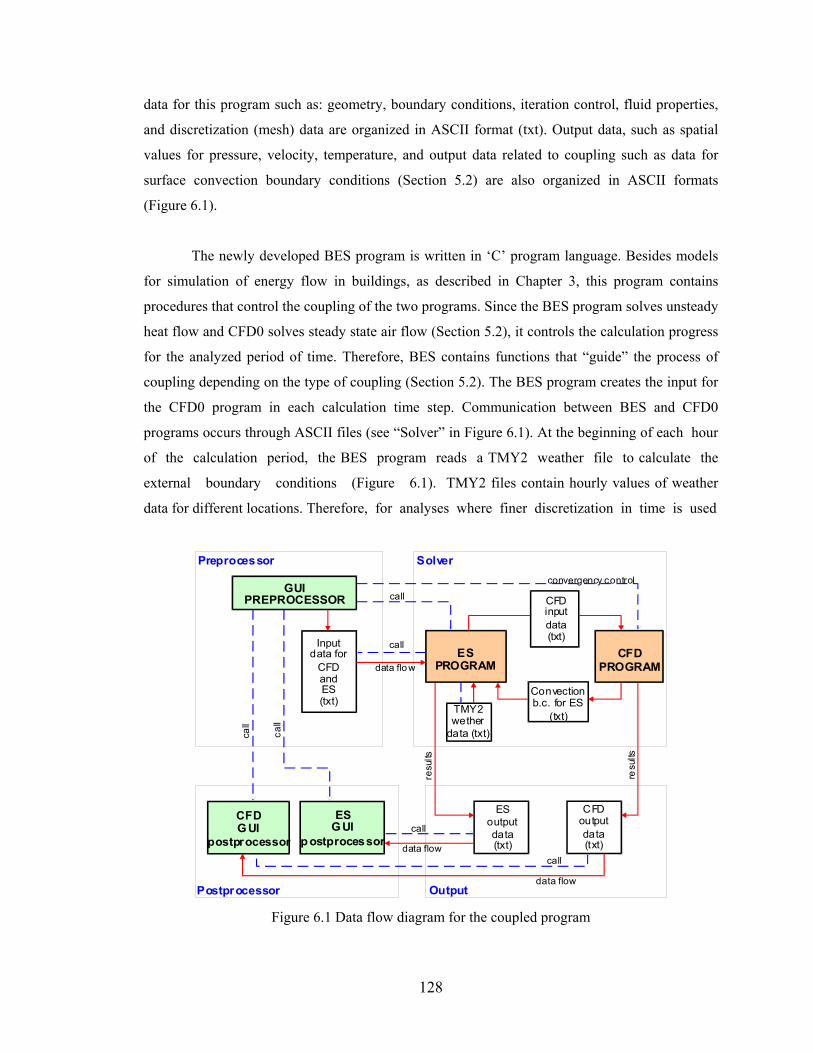
128

data for this program such as: geometry, boundary conditions, iteration control, fluid properties,

and discretization (mesh) data are organized in ASCII format (txt). Output data, such as spatial

values for pressure, velocity, temperature, and output data related to coupling such as data for

surface convection boundary conditions (Section 5.2) are also organized in ASCII formats

(Figure 6.1).

The newly developed BES program is written in ‘C’ program language. Besides models

for simulation of energy flow in buildings, as described in Chapter 3, this program contains

procedures that control the coupling of the two programs. Since the BES program solves unsteady

heat flow and CFD0 solves steady state air flow (Section 5.2), it controls the calculation progress

for the analyzed period of time. Therefore, BES contains functions that “guide” the process of

coupling depending on the type of coupling (Section 5.2). The BES program creates the input for

the CFD0 program in each calculation time step. Communication between BES and CFD0

programs occurs through ASCII files (see “Solver” in Figure 6.1). At the beginning of each hour

of the calculation period, the BES program reads a TMY2 weather file to calculate the

external boundary conditions (Figure 6.1). TMY2 files contain hourly values of weather

data for different locations. Therefore, for analyses where finer discretization in time is used

GUIPREPROCESSOR

ESPROGRAM

CFDPROGRAM

CFDinputdata(txt)

Convectionb.c. for ES

(txt)TMY2wether

data (txt)

CFDG UI

postprocessor

ESG UI

postprocessor

Inputdata for

CFDandES(txt)

call

data flo w

call

call

call

call

data flowcall

data flow

ESoutputdata(txt)

CFDoutputdata(txt)

convergency control

Postprocessor Output

Preprocessor Solver

resu

lts

resu

lts

Figure 6.1 Data flow diagram for the coupled program

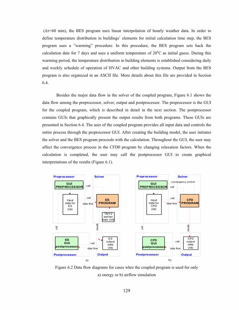
129

(∆τ<60 min), the BES program uses linear interpolation of hourly weather data. In order to

define temperature distribution in buildings’ elements for initial calculation time step, the BES

program uses a ”warming” procedure. In this procedure, the BES program sets back the

calculation date for 7 days and uses a uniform temperature of 20oC as initial guess. During this

warming period, the temperature distribution in building elements is established considering daily

and weekly schedule of operation of HVAC and other building systems. Output from the BES

program is also organized in an ASCII file. More details about this file are provided in Section

6.4.

Besides the major data flow in the solver of the coupled program, Figure 6.1 shows the

data flow among the preprocessor, solver, output and postprocessor. The preprocessor is the GUI

for the coupled program, which is described in detail in the next section. The postprocessor

contains GUIs that graphically present the output results from both programs. These GUIs are

presented in Section 6.4. The user of the coupled program provides all input data and controls the

entire process through the preprocessor GUI. After creating the building model, the user initiates

the solver and the BES program proceeds with the calculation. Throughout the GUI, the user may

affect the convergence process in the CFD0 program by changing relaxation factors. When the

calculation is completed, the user may call the postprocessor GUI to create graphical

interpretations of the results (Figure 6.1).

GUIPREPROCESSOR

ESPROGRAM

TMY2wether

data (txt)

ESGUI

postprocessor

Inputdata for

ES(txt)

call

data flow

call

call

call

data flow

ESoutputdata(txt)

Postprocessor Output

Preprocessor Solver

resu

lts

GUIPREPROCESSOR

CFDPROGRAM

CFDGUI

postprocessor

Inputdata for

CFD(txt)

call

data flow

call

call

call

data flow

CFDoutputdata(txt)

convergency control

Postprocessor Output

Preprocessor Solver

resu

lts

a) b) Figure 6.2 Data flow diagrams for cases whre the coupled program is used for only

a) energy or b) airflow simulation

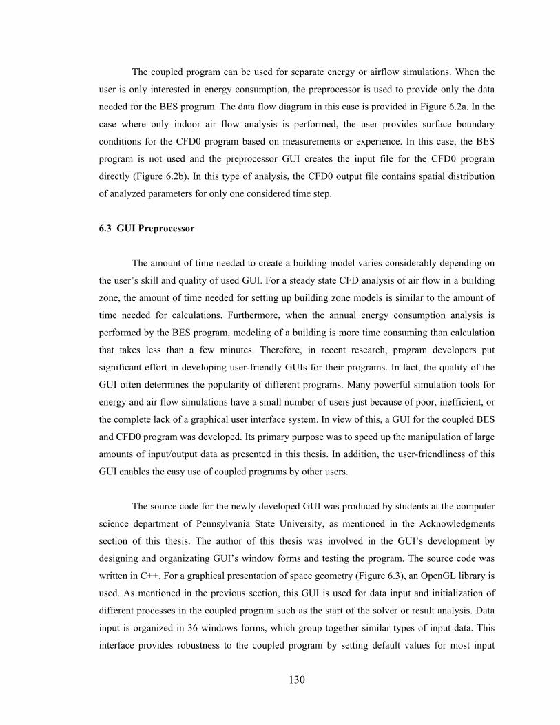
130

The coupled program can be used for separate energy or airflow simulations. When the

user is only interested in energy consumption, the preprocessor is used to provide only the data

needed for the BES program. The data flow diagram in this case is provided in Figure 6.2a. In the

case where only indoor air flow analysis is performed, the user provides surface boundary

conditions for the CFD0 program based on measurements or experience. In this case, the BES

program is not used and the preprocessor GUI creates the input file for the CFD0 program

directly (Figure 6.2b). In this type of analysis, the CFD0 output file contains spatial distribution

of analyzed parameters for only one considered time step.

6.3 GUI Preprocessor

The amount of time needed to create a building model varies considerably depending on

the user’s skill and quality of used GUI. For a steady state CFD analysis of air flow in a building

zone, the amount of time needed for setting up building zone models is similar to the amount of

time needed for calculations. Furthermore, when the annual energy consumption analysis is

performed by the BES program, modeling of a building is more time consuming than calculation

that takes less than a few minutes. Therefore, in recent research, program developers put

significant effort in developing user-friendly GUIs for their programs. In fact, the quality of the

GUI often determines the popularity of different programs. Many powerful simulation tools for

energy and air flow simulations have a small number of users just because of poor, inefficient, or

the complete lack of a graphical user interface system. In view of this, a GUI for the coupled BES

and CFD0 program was developed. Its primary purpose was to speed up the manipulation of large

amounts of input/output data as presented in this thesis. In addition, the user-friendliness of this

GUI enables the easy use of coupled programs by other users.

The source code for the newly developed GUI was produced by students at the computer

science department of Pennsylvania State University, as mentioned in the Acknowledgments

section of this thesis. The author of this thesis was involved in the GUI’s development by

designing and organizating GUI’s window forms and testing the program. The source code was

written in C++. For a graphical presentation of space geometry (Figure 6.3), an OpenGL library is

used. As mentioned in the previous section, this GUI is used for data input and initialization of

different processes in the coupled program such as the start of the solver or result analysis. Data

input is organized in 36 windows forms, which group together similar types of input data. This

interface provides robustness to the coupled program by setting default values for most input

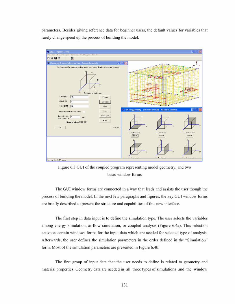
131

parameters. Besides giving reference data for beginner users, the default values for variables that

rarely change speed up the process of building the model.

Figure 6.3 GUI of the coupled program representing model geometry, and two

basic window forms

The GUI window forms are connected in a way that leads and assists the user though the

process of building the model. In the next few paragraphs and figures, the key GUI window forms

are briefly described to present the structure and capabilities of this new interface.

The first step in data input is to define the simulation type. The user selects the variables

among energy simulation, airflow simulation, or coupled analysis (Figure 6.4a). This selection

activates certain windows forms for the input data which are needed for selected type of analysis.

Afterwards, the user defines the simulation parameters in the order defined in the “Simulation”

form. Most of the simulation parameters are presented in Figure 6.4b.

The first group of input data that the user needs to define is related to geometry and

material properties. Geometry data are needed in all three types of simulations and the window

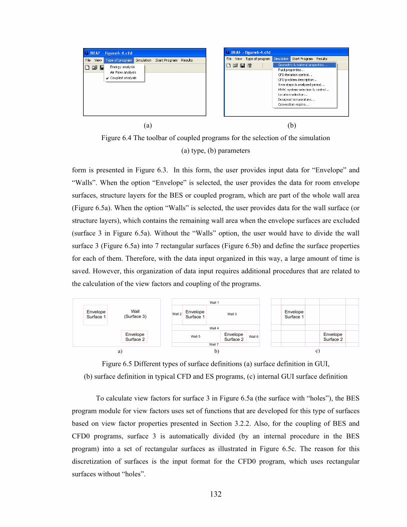
132

(a) (b)

Figure 6.4 The toolbar of coupled programs for the selection of the simulation

(a) type, (b) parameters

form is presented in Figure 6.3. In this form, the user provides input data for “Envelope” and

“Walls”. When the option “Envelope” is selected, the user provides the data for room envelope

surfaces, structure layers for the BES or coupled program, which are part of the whole wall area

(Figure 6.5a). When the option “Walls” is selected, the user provides data for the wall surface (or

structure layers), which contains the remaining wall area when the envelope surfaces are excluded

(surface 3 in Figure 6.5a). Without the “Walls” option, the user would have to divide the wall

surface 3 (Figure 6.5a) into 7 rectangular surfaces (Figure 6.5b) and define the surface properties

for each of them. Therefore, with the data input organized in this way, a large amount of time is

saved. However, this organization of data input requires additional procedures that are related to

the calculation of the view factors and coupling of the programs.

EnvelopeSurface 1

EnvelopeSurface 2

Wall(Surface 3)

EnvelopeSurface 1

EnvelopeSurface 2

Wall 1

Wall 2 Wall 3

Wall 4

Wall 6Wall 5

Wall 7

EnvelopeSurface 1

EnvelopeSurface 2

a) b) c) Figure 6.5 Different types of surface definitions (a) surface definition in GUI,

(b) surface definition in typical CFD and ES programs, (c) internal GUI surface definition

To calculate view factors for surface 3 in Figure 6.5a (the surface with “holes”), the BES

program module for view factors uses set of functions that are developed for this type of surfaces

based on view factor properties presented in Section 3.2.2. Also, for the coupling of BES and

CFD0 programs, surface 3 is automatically divided (by an internal procedure in the BES

program) into a set of rectangular surfaces as illustrated in Figure 6.5c. The reason for this

discretization of surfaces is the input format for the CFD0 program, which uses rectangular

surfaces without “holes”.

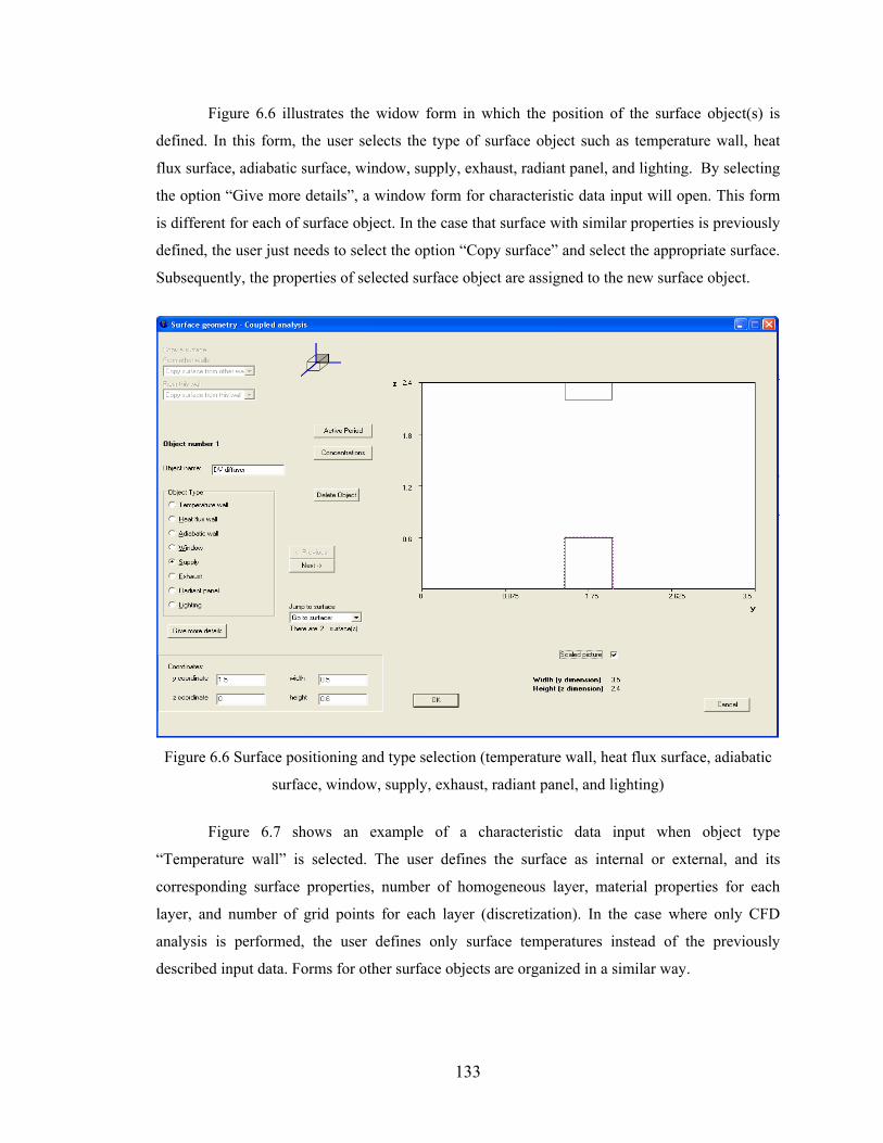
133

Figure 6.6 illustrates the widow form in which the position of the surface object(s) is

defined. In this form, the user selects the type of surface object such as temperature wall, heat

flux surface, adiabatic surface, window, supply, exhaust, radiant panel, and lighting. By selecting

the option “Give more details”, a window form for characteristic data input will open. This form

is different for each of surface object. In the case that surface with similar properties is previously

defined, the user just needs to select the option “Copy surface” and select the appropriate surface.

Subsequently, the properties of selected surface object are assigned to the new surface object.

Figure 6.6 Surface positioning and type selection (temperature wall, heat flux surface, adiabatic

surface, window, supply, exhaust, radiant panel, and lighting)

Figure 6.7 shows an example of a characteristic data input when object type

“Temperature wall” is selected. The user defines the surface as internal or external, and its

corresponding surface properties, number of homogeneous layer, material properties for each

layer, and number of grid points for each layer (discretization). In the case where only CFD

analysis is performed, the user defines only surface temperatures instead of the previously

described input data. Forms for other surface objects are organized in a similar way.

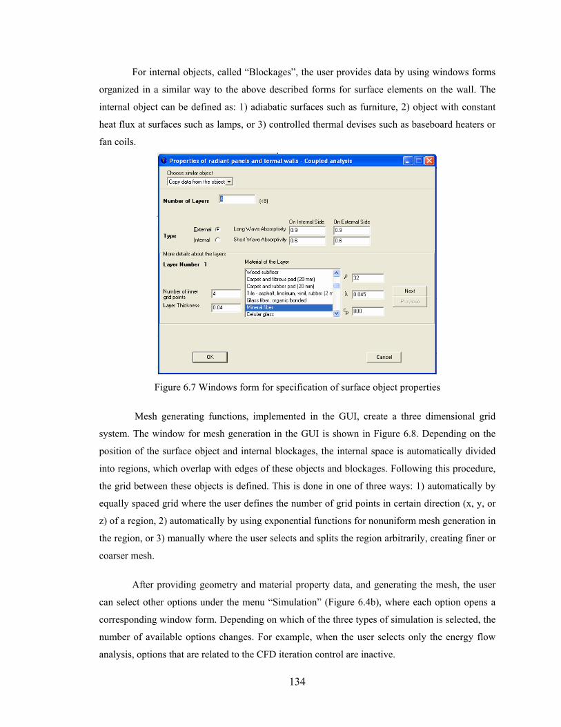
134

For internal objects, called “Blockages”, the user provides data by using windows forms

organized in a similar way to the above described forms for surface elements on the wall. The

internal object can be defined as: 1) adiabatic surfaces such as furniture, 2) object with constant

heat flux at surfaces such as lamps, or 3) controlled thermal devises such as baseboard heaters or

fan coils.

Figure 6.7 Windows form for specification of surface object properties

Mesh generating functions, implemented in the GUI, create a three dimensional grid

system. The window for mesh generation in the GUI is shown in Figure 6.8. Depending on the

position of the surface object and internal blockages, the internal space is automatically divided

into regions, which overlap with edges of these objects and blockages. Following this procedure,

the grid between these objects is defined. This is done in one of three ways: 1) automatically by

equally spaced grid where the user defines the number of grid points in certain direction (x, y, or

z) of a region, 2) automatically by using exponential functions for nonuniform mesh generation in

the region, or 3) manually where the user selects and splits the region arbitrarily, creating finer or

coarser mesh.

After providing geometry and material property data, and generating the mesh, the user

can select other options under the menu “Simulation” (Figure 6.4b), where each option opens a

corresponding window form. Depending on which of the three types of simulation is selected, the

number of available options changes. For example, when the user selects only the energy flow

analysis, options that are related to the CFD iteration control are inactive.

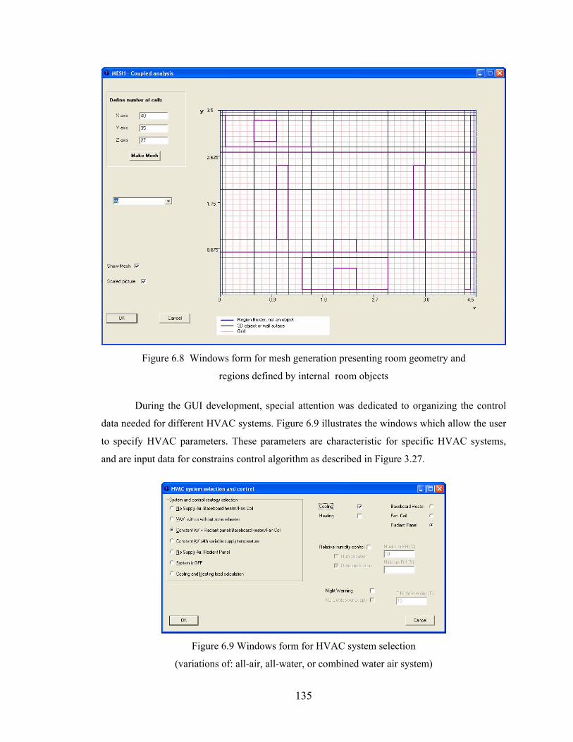
135

Figure 6.8 Windows form for mesh generation presenting room geometry and

regions defined by internal room objects

During the GUI development, special attention was dedicated to organizing the control

data needed for different HVAC systems. Figure 6.9 illustrates the windows which allow the user

to specify HVAC parameters. These parameters are characteristic for specific HVAC systems,

and are input data for constrains control algorithm as described in Figure 3.27.

Figure 6.9 Windows form for HVAC system selection

(variations of: all-air, all-water, or combined water air system)

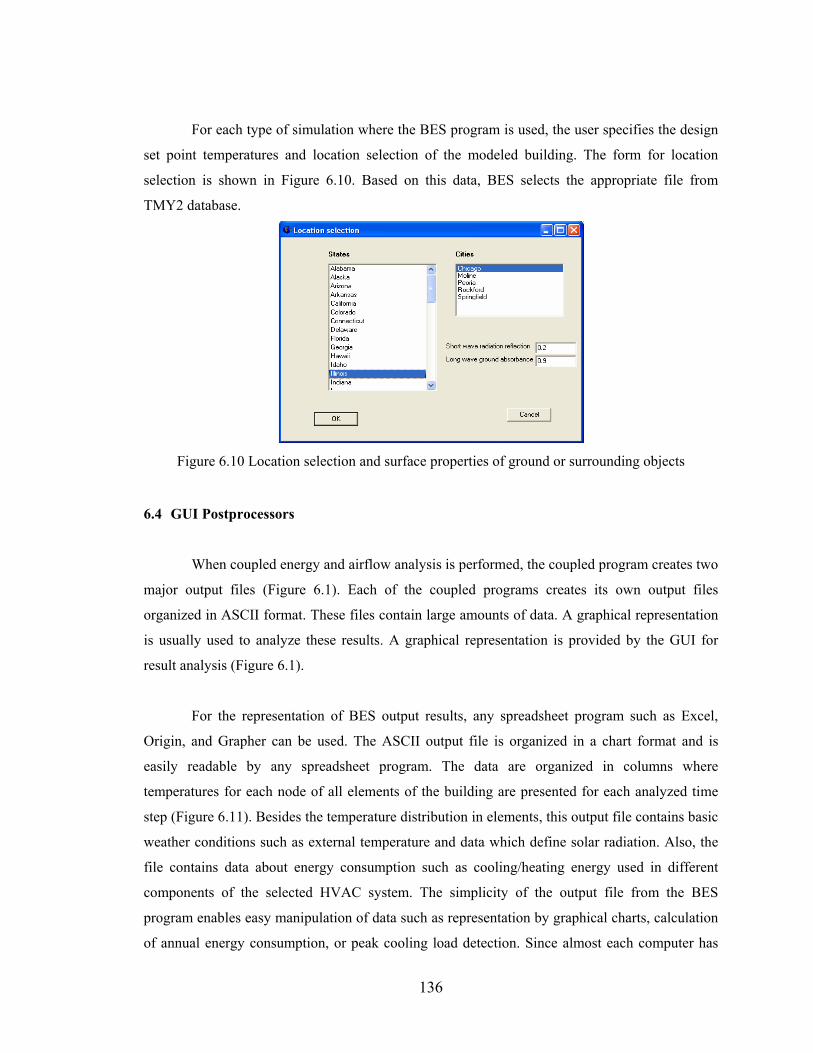
136

For each type of simulation where the BES program is used, the user specifies the design

set point temperatures and location selection of the modeled building. The form for location

selection is shown in Figure 6.10. Based on this data, BES selects the appropriate file from

TMY2 database.

Figure 6.10 Location selection and surface properties of ground or surrounding objects

6.4 GUI Postprocessors

When coupled energy and airflow analysis is performed, the coupled program creates two

major output files (Figure 6.1). Each of the coupled programs creates its own output files

organized in ASCII format. These files contain large amounts of data. A graphical representation

is usually used to analyze these results. A graphical representation is provided by the GUI for

result analysis (Figure 6.1).

For the representation of BES output results, any spreadsheet program such as Excel,

Origin, and Grapher can be used. The ASCII output file is organized in a chart format and is

easily readable by any spreadsheet program. The data are organized in columns where

temperatures for each node of all elements of the building are presented for each analyzed time

step (Figure 6.11). Besides the temperature distribution in elements, this output file contains basic

weather conditions such as external temperature and data which define solar radiation. Also, the

file contains data about energy consumption such as cooling/heating energy used in different

components of the selected HVAC system. The simplicity of the output file from the BES

program enables easy manipulation of data such as representation by graphical charts, calculation

of annual energy consumption, or peak cooling load detection. Since almost each computer has

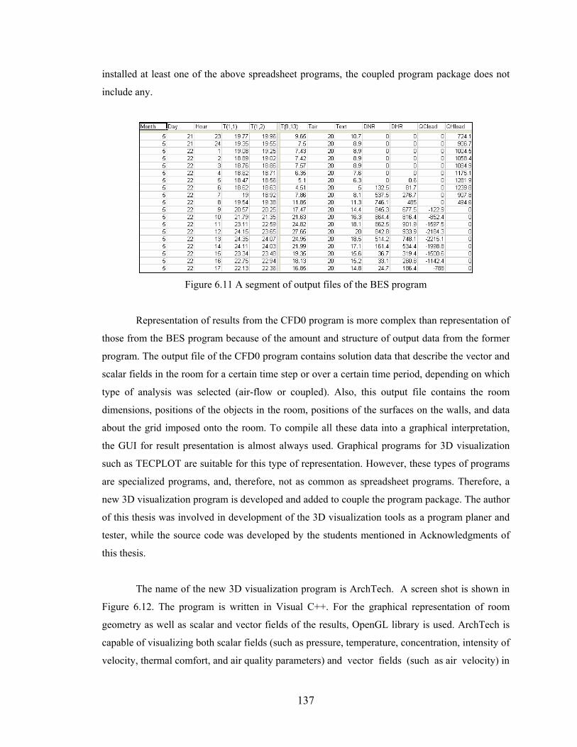
137

installed at least one of the above spreadsheet programs, the coupled program package does not

include any.

Figure 6.11 A segment of output files of the BES program

Representation of results from the CFD0 program is more complex than representation of

those from the BES program because of the amount and structure of output data from the former

program. The output file of the CFD0 program contains solution data that describe the vector and

scalar fields in the room for a certain time step or over a certain time period, depending on which

type of analysis was selected (air-flow or coupled). Also, this output file contains the room

dimensions, positions of the objects in the room, positions of the surfaces on the walls, and data

about the grid imposed onto the room. To compile all these data into a graphical interpretation,

the GUI for result presentation is almost always used. Graphical programs for 3D visualization

such as TECPLOT are suitable for this type of representation. However, these types of programs

are specialized programs, and, therefore, not as common as spreadsheet programs. Therefore, a

new 3D visualization program is developed and added to couple the program package. The author

of this thesis was involved in development of the 3D visualization tools as a program planer and

tester, while the source code was developed by the students mentioned in Acknowledgments of

this thesis.

The name of the new 3D visualization program is ArchTech. A screen shot is shown in

Figure 6.12. The program is written in Visual C++. For the graphical representation of room

geometry as well as scalar and vector fields of the results, OpenGL library is used. ArchTech is

capable of visualizing both scalar fields (such as pressure, temperature, concentration, intensity of

velocity, thermal comfort, and air quality parameters) and vector fields (such as air velocity) in

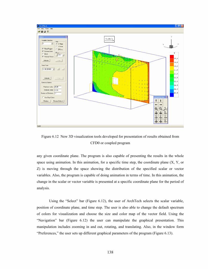
138

Figure 6.12 New 3D visualization tools developed for presentation of results obtained from

CFD0 or coupled program

any given coordinate plane. The program is also capable of presenting the results in the whole

space using animation. In this animation, for a specific time step, the coordinate plane (X, Y, or

Z) is moving through the space showing the distribution of the specified scalar or vector

variables. Also, the program is capable of doing animation in terms of time. In this animation, the

change in the scalar or vector variable is presented at a specific coordinate plane for the period of

analysis.

Using the “Select” bar (Figure 6.12), the user of ArchTech selects the scalar variable,

position of coordinate plane, and time step. The user is also able to change the default spectrum

of colors for visualization and choose the size and color map of the vector field. Using the

“Navigation” bar (Figure 6.12) the user can manipulate the graphical presentation. This

manipulation includes zooming in and out, rotating, and translating. Also, in the window form

“Preferences,” the user sets up different graphical parameters of the program (Figure 6.13).

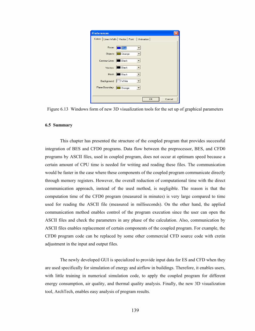
139

Figure 6.13 Windows form of new 3D visualization tools for the set up of graphical parameters

6.5 Summary

This chapter has presented the structure of the coupled program that provides successful

integration of BES and CFD0 programs. Data flow between the preprocessor, BES, and CFD0

programs by ASCII files, used in coupled program, does not occur at optimum speed because a

certain amount of CPU time is needed for writing and reading these files. The communication

would be faster in the case where these components of the coupled program communicate directly

through memory registers. However, the overall reduction of computational time with the direct

communication approach, instead of the used method, is negligible. The reason is that the

computation time of the CFD0 program (measured in minutes) is very large compared to time

used for reading the ASCII file (measured in milliseconds). On the other hand, the applied

communication method enables control of the program execution since the user can open the

ASCII files and check the parameters in any phase of the calculation. Also, communication by

ASCII files enables replacement of certain components of the coupled program. For example, the

CFD0 program code can be replaced by some other commercial CFD source code with cretin

adjustment in the input and output files.

The newly developed GUI is specialized to provide input data for ES and CFD when they

are used specifically for simulation of energy and airflow in buildings. Therefore, it enables users,

with little training in numerical simulation code, to apply the coupled program for different

energy consumption, air quality, and thermal quality analysis. Finally, the new 3D visualization

tool, ArchTech, enables easy analysis of program results.

140

CHAPTER 7

DEVELOPMENT OF NEW CONVECTION CORRELATIONS

7.1 Introduction

Ventilation systems that use displacement ventilation or high aspiration diffusers, with or

without radiant cooling panels, are relatively new and not widely used in building mechanical

systems. As a consequence, convection correlations for surface heat transfer in rooms with these

ventilation systems are still not developed. Until now, convection correlations used with these

types of flow have been based on convection correlations developed for: isolated surfaces, free

edge heated plates, or standard ventilation systems. These convection correlations are used in

various analyses of these two ventilation systems without any explicit experimental validation.

Nevertheless, both displacement and high aspiration diffusers have recently attracted significant

attention of design community due to their performance characteristics; therefore, validated

correlations are needed.

This chapter presents newly developed convection correlations for displacement

ventilation and ventilation with high aspiration diffusers combined with cooled ceiling panels.

First, validity of the existing correlations for considered airflow regimes is investigated.

Afterwards, new convection correlations are developed for surface types and airflow regimes

where validation for the existing correlations fails. These additional convection correlations for

calculation of heat fluxes at internal surfaces are needed to improve performance of MACA

described in Section 4.3. In addition, these correlations can be used with other simulation tools or

in design procedures.

In the next section (Section 7.2) of this chapter, basic details about convection correlation

development are presented. The following sections (Sections 7.3, 7.4, and 7.5) provide results for

newly developed correlations. The final section (Section 7.6) contains general discussion about

these correlations. Detailed reports about the experimental facility, conducted experiments, and

result processing are provided in Chapter 8, together with other details of measurements

conducted as a part of this thesis.

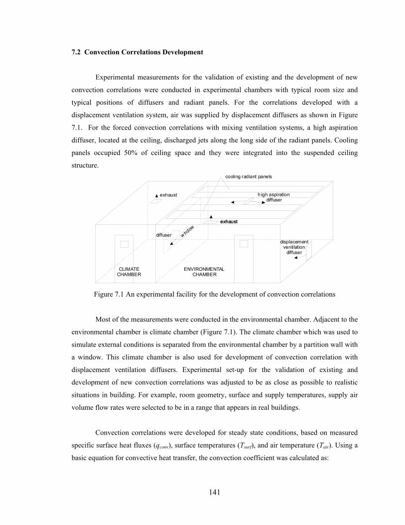
141

7.2 Convection Correlations Development

Experimental measurements for the validation of existing and the development of new

convection correlations were conducted in experimental chambers with typical room size and

typical positions of diffusers and radiant panels. For the correlations developed with a

displacement ventilation system, air was supplied by displacement diffusers as shown in Figure

7.1. For the forced convection correlations with mixing ventilation systems, a high aspiration

diffuser, located at the ceiling, discharged jets along the long side of the radiant panels. Cooling

panels occupied 50% of ceiling space and they were integrated into the suspended ceiling

structure.

ENVIRONMENTAL CHAMBER

CLIMATECHAMBER

h igh aspiration diffuser

exhaust

displacement ventilation

diffuser

exhaust

w indow

cooling radiant panels

diffuser

exhaust

Figure 7.1 An experimental facility for the development of convection correlations

Most of the measurements were conducted in the environmental chamber. Adjacent to the

environmental chamber is climate chamber (Figure 7.1). The climate chamber which was used to

simulate external conditions is separated from the environmental chamber by a partition wall with

a window. This climate chamber is also used for development of convection correlation with

displacement ventilation diffusers. Experimental set-up for the validation of existing and

development of new convection correlations was adjusted to be as close as possible to realistic

situations in building. For example, room geometry, surface and supply temperatures, supply air

volume flow rates were selected to be in a range that appears in real buildings.

Convection correlations were developed for steady state conditions, based on measured

specific surface heat fluxes (qconv), surface temperatures (Tsurf), and air temperature (Tair). Using a

basic equation for convective heat transfer, the convection coefficient was calculated as:

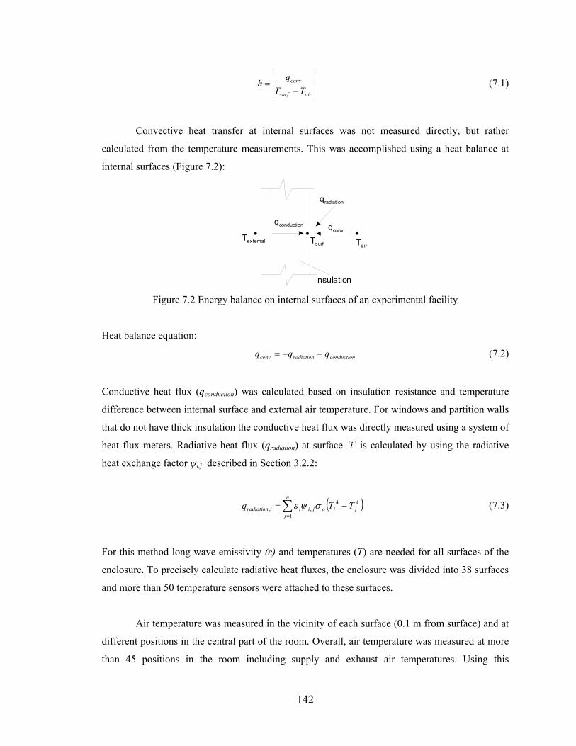
142

airsurf

conv

TTq

h−

= (7.1)

Convective heat transfer at internal surfaces was not measured directly, but rather

calculated from the temperature measurements. This was accomplished using a heat balance at

internal surfaces (Figure 7.2):

Tsurf TairTexternal

qconv

qradiation

qconduction

insulation Figure 7.2 Energy balance on internal surfaces of an experimental facility

Heat balance equation:

conductionradiationconv qqq −−= (7.2)

Conductive heat flux (qconduction) was calculated based on insulation resistance and temperature

difference between internal surface and external air temperature. For windows and partition walls

that do not have thick insulation the conductive heat flux was directly measured using a system of

heat flux meters. Radiative heat flux (qradiation) at surface ‘i’ is calculated by using the radiative

heat exchange factor ψi,j described in Section 3.2.2:

( )∑=

−=n

jjiojiiiradiation TTq

1

44,, σψε (7.3)

For this method long wave emissivity (ε) and temperatures (T) are needed for all surfaces of the

enclosure. To precisely calculate radiative heat fluxes, the enclosure was divided into 38 surfaces

and more than 50 temperature sensors were attached to these surfaces.

Air temperature was measured in the vicinity of each surface (0.1 m from surface) and at

different positions in the central part of the room. Overall, air temperature was measured at more

than 45 positions in the room including supply and exhaust air temperatures. Using this

143

temperature distribution, natural convection correlations at surfaces were calculated for local air

temperature. For surfaces with dominant forced convection, the correlation was expressed as a

function of number of Air Changes per Hour in the room (ACH) using the local air temperature as

the reference temperature.

Convection correlations developed as a part of this thesis are presented in a simplified

form. General relationships between Nusselt numbers (Nu), Prandtl numbers (Pr), and Grashof

numbers (Gr) are defined differently for laminar and turbulent flows (ASHRAE 2001). These

equations are:

For laminar flow: ( ) 4/1Pr⋅= GrCNu L (7.4)

For turbulent flow: ( ) 3/1Pr⋅= GrCNu T (7.5)

By substituting values for constant Pr for air, and other air constants in the expressions for Nu

and Gr numbers, simplified forms for convection correlations are obtained:

( ) 4/1

min_ / LTah arlac ∆= (7.6)

( ) 3/1_ Tbh turbulentc ∆= (7.7)

The Rayleigh number (Ra= Gr.Pr) is used as a criterion to define if the flow is laminar or

turbulent.

For forced convection and turbulent flow:

3/15/4 PrReTCNu = (7.8)

Nusselt and Reynolds numbers can be expressed as functions of room volume (Vroom) and air

supply volume flow rate ( supply.

V ):

air

room

khVNu

3/1

= (7.9)

31 /roomair

supply.

VVReν

= (7.10)

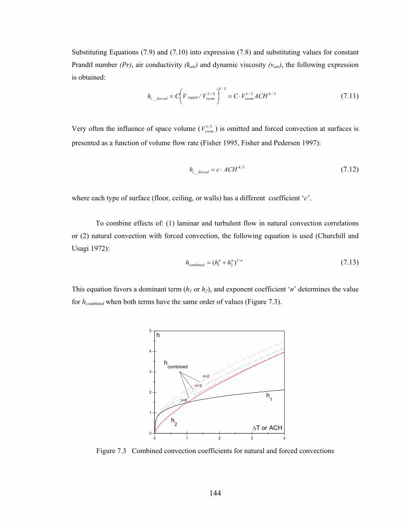
144

Substituting Equations (7.9) and (7.10) into expression (7.8) and substituting values for constant

Prandtl number (Pr), air conductivity (kair) and dynamic viscosity (νair), the following expression

is obtained:

545154

43 //room

//

roomsupply.

forced_c ACHVCV/VCh ⋅=

= (7.11)

Very often the influence of space volume ( 5/1roomV ) is omitted and forced convection at surfaces is

presented as a function of volume flow rate (Fisher 1995, Fisher and Pedersen 1997):

5/4

_ ACHch forcedc ⋅= (7.12)

where each type of surface (floor, ceiling, or walls) has a different coefficient ‘c’.

To combine effects of: (1) laminar and turbulent flow in natural convection correlations

or (2) natural convection with forced convection, the following equation is used (Churchill and

Usagi 1972): nnn

combined hhh /121 )( += (7.13)

This equation favors a dominant term (h1 or h2), and exponent coefficient ‘n’ determines the value

for hcombined when both terms have the same order of values (Figure 7.3).

0 1 2 3 40

1

2

3

4

5h

∆T or ACH

n=2

n=3

n=6

h2

h1

hcombined

Figure 7.3 Combined convection coefficients for natural and forced convections

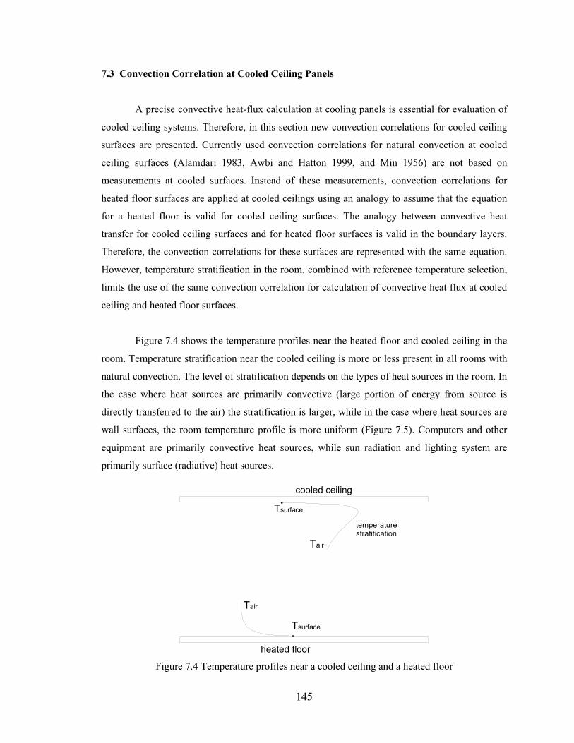
145

7.3 Convection Correlation at Cooled Ceiling Panels

A precise convective heat-flux calculation at cooling panels is essential for evaluation of

cooled ceiling systems. Therefore, in this section new convection correlations for cooled ceiling

surfaces are presented. Currently used convection correlations for natural convection at cooled

ceiling surfaces (Alamdari 1983, Awbi and Hatton 1999, and Min 1956) are not based on

measurements at cooled surfaces. Instead of these measurements, convection correlations for

heated floor surfaces are applied at cooled ceilings using an analogy to assume that the equation

for a heated floor is valid for cooled ceiling surfaces. The analogy between convective heat

transfer for cooled ceiling surfaces and for heated floor surfaces is valid in the boundary layers.

Therefore, the convection correlations for these surfaces are represented with the same equation.

However, temperature stratification in the room, combined with reference temperature selection,

limits the use of the same convection correlation for calculation of convective heat flux at cooled

ceiling and heated floor surfaces.

Figure 7.4 shows the temperature profiles near the heated floor and cooled ceiling in the

room. Temperature stratification near the cooled ceiling is more or less present in all rooms with

natural convection. The level of stratification depends on the types of heat sources in the room. In

the case where heat sources are primarily convective (large portion of energy from source is

directly transferred to the air) the stratification is larger, while in the case where heat sources are

wall surfaces, the room temperature profile is more uniform (Figure 7.5). Computers and other

equipment are primarily convective heat sources, while sun radiation and lighting system are

primarily surface (radiative) heat sources.

cooled ceiling

heated floor

Tsurface

Tsurface

Tair

temperature stratification

Tair

Figure 7.4 Temperature profiles near a cooled ceiling and a heated floor

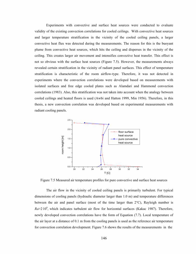
146

Experiments with convective and surface heat sources were conducted to evaluate

validity of the existing convection correlations for cooled ceilings. With convective heat sources

and larger temperature stratification in the vicinity of the cooled ceiling panels, a larger

convective heat flux was detected during the measurements. The reason for this is the buoyant

plume from convective heat sources, which hits the ceiling and disperses in the vicinity of the

ceiling. This creates larger air movement and intensifies convective heat transfer. This effect is

not so obvious with the surface heat sources (Figure 7.5). However, the measurements always

revealed certain stratification in the vicinity of radiant panel surfaces. This effect of temperature

stratification is characteristic of the room airflow-type. Therefore, it was not detected in

experiments where the convection correlations were developed based on measurements with

isolated surfaces and free edge cooled plates such as Alamdari and Hammond convection

correlations (1983). Also, this stratification was not taken into account when the analogy between

cooled ceilings and heated floors is used (Awbi and Hatton 1999, Min 1956). Therefore, in this

thesis, a new convection correlation was developed based on experimental measurements with

radiant cooling panels.

20 22 24 26 28 30 32 340.0

0.5

1.0

1.5

2.0

2.5

floor surface heat source

pure convective heat source

room

hei

ght [

m]

T [C] Figure 7.5 Measured air temperature profiles for pure convective and surface heat sources

The air flow in the vicinity of cooled ceiling panels is primarily turbulent. For typical

dimensions of cooling panels (hydraulic diameter larger than 1.0 m) and temperature differences

between the air and panel surface (most of the time larger than 2°C), Rayleigh number is

Ra>2.108, which indicates turbulent air flow for horizontal surfaces (Kakac 1987). Therefore,

newly developed convection correlations have the form of Equation (7.7). Local temperature of

the air layer at a distance of 0.1 m from the cooling panels is used as the reference air temperature

for convection correlation development. Figure 7.6 shows the results of the measurements in the

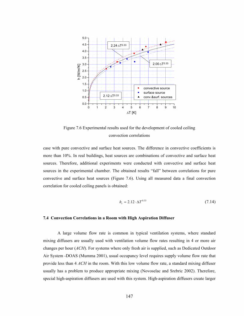
147

0 1 2 3 4 5 6 7 8 9 100.0

0.5

1.0

1.5

2.0

2.5

3.0

3.5

4.0

4.5

5.0

2.00.∆T0.33

2.12.∆T0.33

2.24.∆T0.33

convective source surface source conv.&surf. sources

h [W

/m2 K

]

∆T [K]

Figure 7.6 Experimental results used for the development of cooled ceiling

convection correlations

case with pure convective and surface heat sources. The difference in convective coefficients is

more than 10%. In real buildings, heat sources are combinations of convective and surface heat

sources. Therefore, additional experiments were conducted with convective and surface heat

sources in the experimental chamber. The obtained results “fall” between correlations for pure

convective and surface heat sources (Figure 7.6). Using all measured data a final convection

correlation for cooled ceiling panels is obtained:

33.012.2 Thc ∆⋅= (7.14)

7.4 Convection Correlations in a Room with High Aspiration Diffuser

A large volume flow rate is common in typical ventilation systems, where standard

mixing diffusers are usually used with ventilation volume flow rates resulting in 4 or more air

changes per hour (ACH). For systems where only fresh air is supplied, such as Dedicated Outdoor

Air System -DOAS (Mumma 2001), usual occupancy level requires supply volume flow rate that

provide less than 4 ACH in the room. With this low volume flow rate, a standard mixing diffuser

usually has a problem to produce appropriate mixing (Novoselac and Srebric 2002). Therefore,

special high-aspiration diffusers are used with this system. High-aspiration diffusers create larger

148

mixing with the same primary volume flow rate. Therefore, different correlations are expected for

this type of flow when compared to the flow for Fisher and Pedersen’s correlations (1995, 1997).

In addition, rooms with cooled ceilings have enclosure temperature considerably lower than with

other HVAC cooling systems. In these rooms enclosure temperatures are close to the room air

temperature (Novoselac and Srebric 2002) and buoyancy at enclosure surfaces is small.

Therefore, forced convection can be dominant at the majority of surfaces when high-aspiration

diffusers are combined with ceiling cooling panels. To develop convection correlations for rooms

with cooled ceiling and high aspiration diffusers, a new set of experiments with high aspiration

diffuser was conducted.

In the experimental setup a high aspiration diffuser positioned between the radiant panels

supplied the air along the panel’s longer sides (Figure 7.1). As a heat source in the room, a pure

convective heat source was used. Radiant panels extracted the heat directly by convection and

indirectly by radiation. Cooled ceiling panels decreased the temperature of the rest of the

surfaces. In these experiments, all room surfaces had lower temperature than the room air

temperature because the pure convective heat source (with minor radiation effects) was used to

produce cooling load.

To create generalized forced convection correlations, specific volume flow rate

represented by ACH is used to describe the intensity of air movement near surfaces. Therefore,

forced convection correlations have the form of Equation (7.12). As a reference temperature,

local air temperature was selected instead of supply air temperature, which was used by Fisher

and Pedersen (1995, 1997). The high aspiration diffuser creates large air entrainment and jet

temperature becomes close to the room air temperature after a short distance from the diffuser.

Hence, with the high aspiration diffuser, a reference temperature difference between supply air

and surface temperatures that are distant from diffuser would not be relevant.

A high aspiration diffuser combined with a cooled ceiling system supplies constant

volume flow rate. Therefore, during the experiments, air volume flow rate was varied for several

different heat loads in order to get a correlation between ACH and h, while the jet velocity was

kept approximately constant at a face velocity of 15 m/s. The high aspiration diffuser supply

velocity was kept approximately constant by changing the number of supply diffuser openings.

Also, supply temperature was kept constant and approximately equal to the room temperature

because supply temperature has a small effect on forced convection correlation with the high

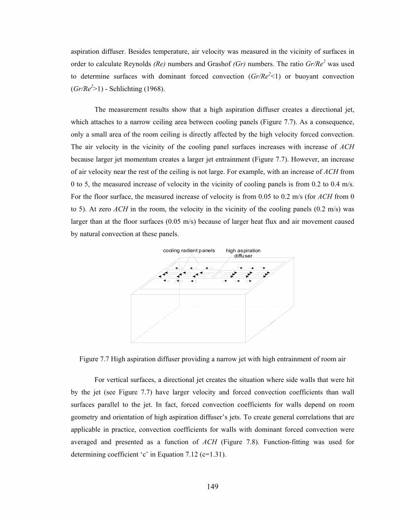
149

aspiration diffuser. Besides temperature, air velocity was measured in the vicinity of surfaces in

order to calculate Reynolds (Re) numbers and Grashof (Gr) numbers. The ratio Gr/Re2 was used

to determine surfaces with dominant forced convection (Gr/Re2<1) or buoyant convection

(Gr/Re2>1) - Schlichting (1968).

The measurement results show that a high aspiration diffuser creates a directional jet,

which attaches to a narrow ceiling area between cooling panels (Figure 7.7). As a consequence,

only a small area of the room ceiling is directly affected by the high velocity forced convection.

The air velocity in the vicinity of the cooling panel surfaces increases with increase of ACH

because larger jet momentum creates a larger jet entrainment (Figure 7.7). However, an increase

of air velocity near the rest of the ceiling is not large. For example, with an increase of ACH from

0 to 5, the measured increase of velocity in the vicinity of cooling panels is from 0.2 to 0.4 m/s.

For the floor surface, the measured increase of velocity is from 0.05 to 0.2 m/s (for ACH from 0

to 5). At zero ACH in the room, the velocity in the vicinity of the cooling panels (0.2 m/s) was

larger than at the floor surfaces (0.05 m/s) because of larger heat flux and air movement caused

by natural convection at these panels.

high aspiration diffuser

cooling radiant panels

Figure 7.7 High aspiration diffuser providing a narrow jet with high entrainment of room air

For vertical surfaces, a directional jet creates the situation where side walls that were hit

by the jet (see Figure 7.7) have larger velocity and forced convection coefficients than wall

surfaces parallel to the jet. In fact, forced convection coefficients for walls depend on room

geometry and orientation of high aspiration diffuser’s jets. To create general correlations that are

applicable in practice, convection coefficients for walls with dominant forced convection were

averaged and presented as a function of ACH (Figure 7.8). Function-fitting was used for

determining coefficient ‘c’ in Equation 7.12 (c=1.31).

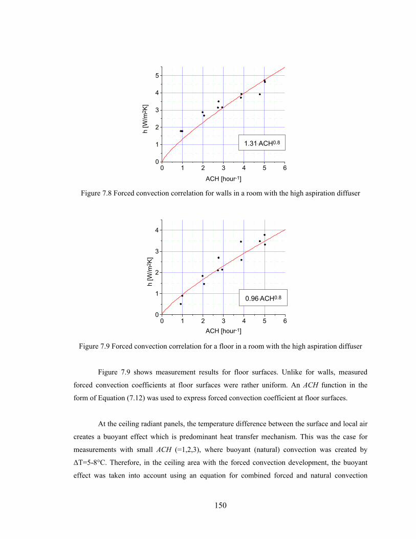
150

0 1 2 3 4 5 60

1

2

3

4

5

1.31.ACH0.8h

[W/m

2 K]

ACH [hour-1] Figure 7.8 Forced convection correlation for walls in a room with the high aspiration diffuser

0 1 2 3 4 5 60

1

2

3

4

0.96.ACH0.8

h [W

/m2 K

]

ACH [hour-1] Figure 7.9 Forced convection correlation for a floor in a room with the high aspiration diffuser

Figure 7.9 shows measurement results for floor surfaces. Unlike for walls, measured

forced convection coefficients at floor surfaces were rather uniform. An ACH function in the

form of Equation (7.12) was used to express forced convection coefficient at floor surfaces.

At the ceiling radiant panels, the temperature difference between the surface and local air

creates a buoyant effect which is predominant heat transfer mechanism. This was the case for

measurements with small ACH (=1,2,3), where buoyant (natural) convection was created by

∆T=5-8°C. Therefore, in the ceiling area with the forced convection development, the buoyant

effect was taken into account using an equation for combined forced and natural convection

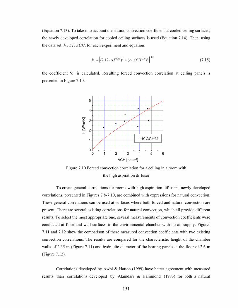
151

(Equation 7.13). To take into account the natural convection coefficient at cooled ceiling surfaces,

the newly developed correlation for cooled ceiling surfaces is used (Equation 7.14). Then, using

the data set: hc, ∆T, ACH, for each experiment and equation:

[ ] 3/138.0333.0 )()12.2( ACHcThc ⋅+∆⋅= (7.15)

the coefficient ‘c’ is calculated. Resulting forced convection correlation at ceiling panels is

presented in Figure 7.10.

0 1 2 3 4 5 60

1

2

3

4

5

1.19.ACH0.8

h [W

/m2 K

]

ACH [hour-1] Figure 7.10 Forced convection correlation for a ceiling in a room with

the high aspiration diffuser

To create general correlations for rooms with high aspiration diffusers, newly developed

correlations, presented in Figures 7.8-7.10, are combined with expressions for natural convection.

These general correlations can be used at surfaces where both forced and natural convection are

present. There are several existing correlations for natural convection, which all provide different

results. To select the most appropriate one, several measurements of convection coefficients were

conducted at floor and wall surfaces in the environmental chamber with no air supply. Figures

7.11 and 7.12 show the comparison of these measured convection coefficients with two existing

convection correlations. The results are compared for the characteristic height of the chamber

walls of 2.35 m (Figure 7.11) and hydraulic diameter of the heating panels at the floor of 2.6 m

(Figure 7.12).

Correlations developed by Awbi & Hatton (1999) have better agreement with measured

results than correlations developed by Alamdari & Hammond (1983) for both a natural

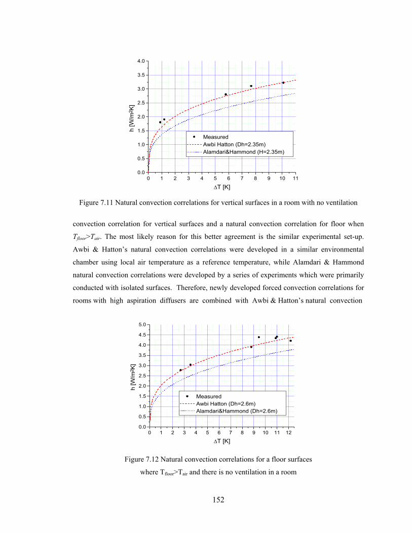
152

0 1 2 3 4 5 6 7 8 9 10 110.0

0.5

1.0

1.5

2.0

2.5

3.0

3.5

4.0

Measured Awbi Hatton (Dh=2.35m) Alamdari&Hammond (H=2.35m)

h [W

/m2 K

]

∆T [K] Figure 7.11 Natural convection correlations for vertical surfaces in a room with no ventilation

convection correlation for vertical surfaces and a natural convection correlation for floor when

Tfloor>Tair. The most likely reason for this better agreement is the similar experimental set-up.

Awbi & Hatton’s natural convection correlations were developed in a similar environmental

chamber using local air temperature as a reference temperature, while Alamdari & Hammond

natural convection correlations were developed by a series of experiments which were primarily

conducted with isolated surfaces. Therefore, newly developed forced convection correlations for

rooms with high aspiration diffusers are combined with Awbi & Hatton’s natural convection

0 1 2 3 4 5 6 7 8 9 10 11 120.0

0.5

1.0

1.5

2.0

2.5

3.0

3.5

4.0

4.5

5.0

Measured Awbi Hatton (Dh=2.6m) Alamdari&Hammond (Dh=2.6m)

h [W

/m2 K

]

∆T [K]

Figure 7.12 Natural convection correlations for a floor surfaces

where Tfloor>Tair and there is no ventilation in a room

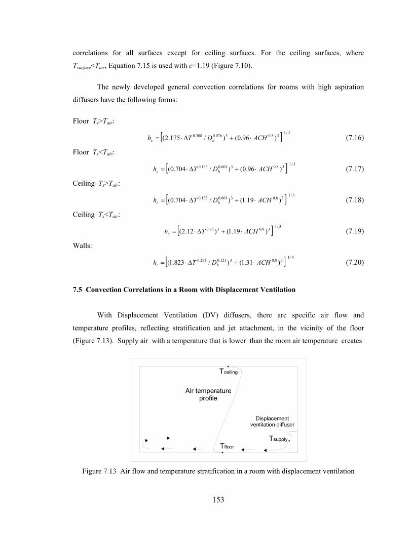
153

correlations for all surfaces except for ceiling surfaces. For the ceiling surfaces, where

Tsurface<Tair, Equation 7.15 is used with c=1.19 (Figure 7.10).

The newly developed general convection correlations for rooms with high aspiration

diffusers have the following forms:

Floor Ts>Tair:

[ ] 3/138.03076.0308.0 )96.0()/175.2( ACHDTh hc ⋅+∆⋅= (7.16)

Floor Ts<Tair:

[ ] 3/138.03601.0133.0 )96.0()/704.0( ACHDTh hc ⋅+∆⋅= (7.17)

Ceiling Ts>Tair:

[ ] 3/138.03601.0133.0 )19.1()/704.0( ACHDTh hc ⋅+∆⋅= (7.18)

Ceiling Ts<Tair:

[ ] 3/138.0333.0 )19.1()12.2( ACHThc ⋅+∆⋅= (7.19)

Walls:

[ ] 3/138.03121.0293.0 )31.1()/823.1( ACHDTh hc ⋅+∆⋅= (7.20)

7.5 Convection Correlations in a Room with Displacement Ventilation

With Displacement Ventilation (DV) diffusers, there are specific air flow and

temperature profiles, reflecting stratification and jet attachment, in the vicinity of the floor

(Figure 7.13). Supply air with a temperature that is lower than the room air temperature creates

TsupplyTfloor

Tceiling

Air temperature profile

Displacement ventilation diffuser

Figure 7.13 Air flow and temperature stratification in a room with displacement ventilation

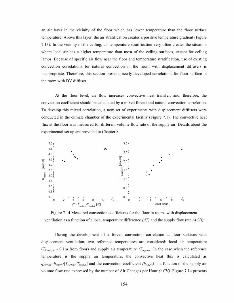
154

an air layer in the vicinity of the floor which has lower temperature than the floor surface

temperature. Above this layer, the air stratification creates a positive temperature gradient (Figure

7.13). In the vicinity of the ceiling, air temperature stratification very often creates the situation

where local air has a higher temperature than most of the ceiling surfaces, except for ceiling

lamps. Because of specific air flow near the floor and temperature stratification, use of existing

convection correlations for natural convection in the room with displacement diffusers is

inappropriate. Therefore, this section presents newly developed correlations for floor surface in

the room with DV diffuser.

At the floor level, air flow increases convective heat transfer, and, therefore, the

convection coefficient should be calculated by a mixed forced and natural convection correlation.

To develop this mixed correlation, a new set of experiments with displacement diffusers were

conducted in the climate chamber of the experimental facility (Figure 7.1). The convective heat

flux at the floor was measured for different volume flow rate of the supply air. Details about the

experimental set up are provided in Chapter 8.

0 2 4 6 8 10 120.0

0.5

1.0

1.5

2.0

2.5

3.0

3.5

4.0

4.5

5.0

ACH [hour-1]

h lo

cal ∆

T [W

/m2 K

]

∆T = Tsurface

-Tlocal air

[oC]

0 2 4 6 8 100.0

0.5

1.0

1.5

2.0

2.5

3.0

h su

pply

∆T [

W/m

2 K]

Figure 7.14 Measured convection coefficients for the floor in rooms with displacement

ventilation as a function of a local temperature difference (∆T) and the supply flow rate (ACH)

During the development of a forced convection correlation at floor surfaces with

displacement ventilation, two reference temperatures are considered: local air temperature

(Tlocal_air - 0.1m from floor) and supply air temperature (Tsupply). In the case when the reference

temperature is the supply air temperature, the convective heat flux is calculated as

qsurface=hsupply·[Tsurface-Tsupply] and the convection coefficient (hsupply) is a function of the supply air

volume flow rate expressed by the number of Air Changes per Hour (ACH). Figure 7.14 presents

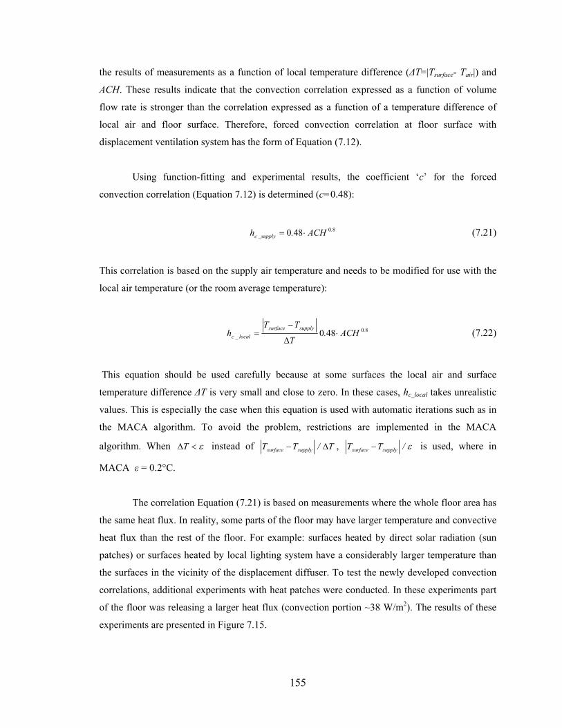
155

the results of measurements as a function of local temperature difference (∆T=|Tsurface- Tair|) and

ACH. These results indicate that the convection correlation expressed as a function of volume

flow rate is stronger than the correlation expressed as a function of a temperature difference of

local air and floor surface. Therefore, forced convection correlation at floor surface with

displacement ventilation system has the form of Equation (7.12).

Using function-fitting and experimental results, the coefficient ‘c’ for the forced

convection correlation (Equation 7.12) is determined (c=0.48):

80480 .

_supplyc ACH.h ⋅= (7.21)

This correlation is based on the supply air temperature and needs to be modified for use with the

local air temperature (or the room average temperature):

80480 .supplysurfacelocal_c ACH.

T

TTh ⋅

∆

−= (7.22)

This equation should be used carefully because at some surfaces the local air and surface

temperature difference ∆T is very small and close to zero. In these cases, hc_local takes unrealistic

values. This is especially the case when this equation is used with automatic iterations such as in

the MACA algorithm. To avoid the problem, restrictions are implemented in the MACA

algorithm. When ε<∆T instead of T/TT supplysurface ∆− , ε/TT supplysurface − is used, where in

MACA ε = 0.2°C.

The correlation Equation (7.21) is based on measurements where the whole floor area has

the same heat flux. In reality, some parts of the floor may have larger temperature and convective

heat flux than the rest of the floor. For example: surfaces heated by direct solar radiation (sun

patches) or surfaces heated by local lighting system have a considerably larger temperature than

the surfaces in the vicinity of the displacement diffuser. To test the newly developed convection

correlations, additional experiments with heat patches were conducted. In these experiments part

of the floor was releasing a larger heat flux (convection portion ~38 W/m2). The results of these

experiments are presented in Figure 7.15.

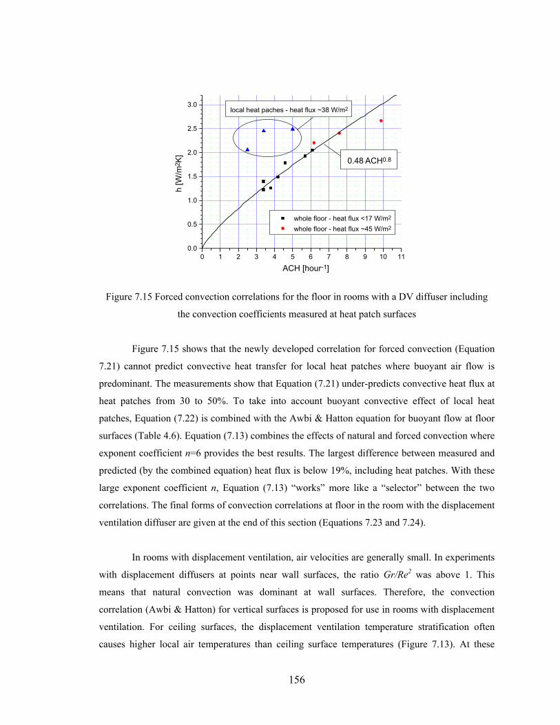
156

0 1 2 3 4 5 6 7 8 9 10 110.0

0.5

1.0

1.5

2.0

2.5

3.0

ACH [hour-1]

local heat paches - heat flux ~38 W/m2

h [W

/m2 K

]

whole floor - heat flux <17 W/m2

whole floor - heat flux ~45 W/m2

0.48.ACH0.8

Figure 7.15 Forced convection correlations for the floor in rooms with a DV diffuser including

the convection coefficients measured at heat patch surfaces

Figure 7.15 shows that the newly developed correlation for forced convection (Equation

7.21) cannot predict convective heat transfer for local heat patches where buoyant air flow is

predominant. The measurements show that Equation (7.21) under-predicts convective heat flux at

heat patches from 30 to 50%. To take into account buoyant convective effect of local heat

patches, Equation (7.22) is combined with the Awbi & Hatton equation for buoyant flow at floor

surfaces (Table 4.6). Equation (7.13) combines the effects of natural and forced convection where

exponent coefficient n=6 provides the best results. The largest difference between measured and

predicted (by the combined equation) heat flux is below 19%, including heat patches. With these

large exponent coefficient n, Equation (7.13) “works” more like a “selector” between the two

correlations. The final forms of convection correlations at floor in the room with the displacement

ventilation diffuser are given at the end of this section (Equations 7.23 and 7.24).

In rooms with displacement ventilation, air velocities are generally small. In experiments

with displacement diffusers at points near wall surfaces, the ratio Gr/Re2 was above 1. This

means that natural convection was dominant at wall surfaces. Therefore, the convection

correlation (Awbi & Hatton) for vertical surfaces is proposed for use in rooms with displacement

ventilation. For ceiling surfaces, the displacement ventilation temperature stratification often

causes higher local air temperatures than ceiling surface temperatures (Figure 7.13). At these

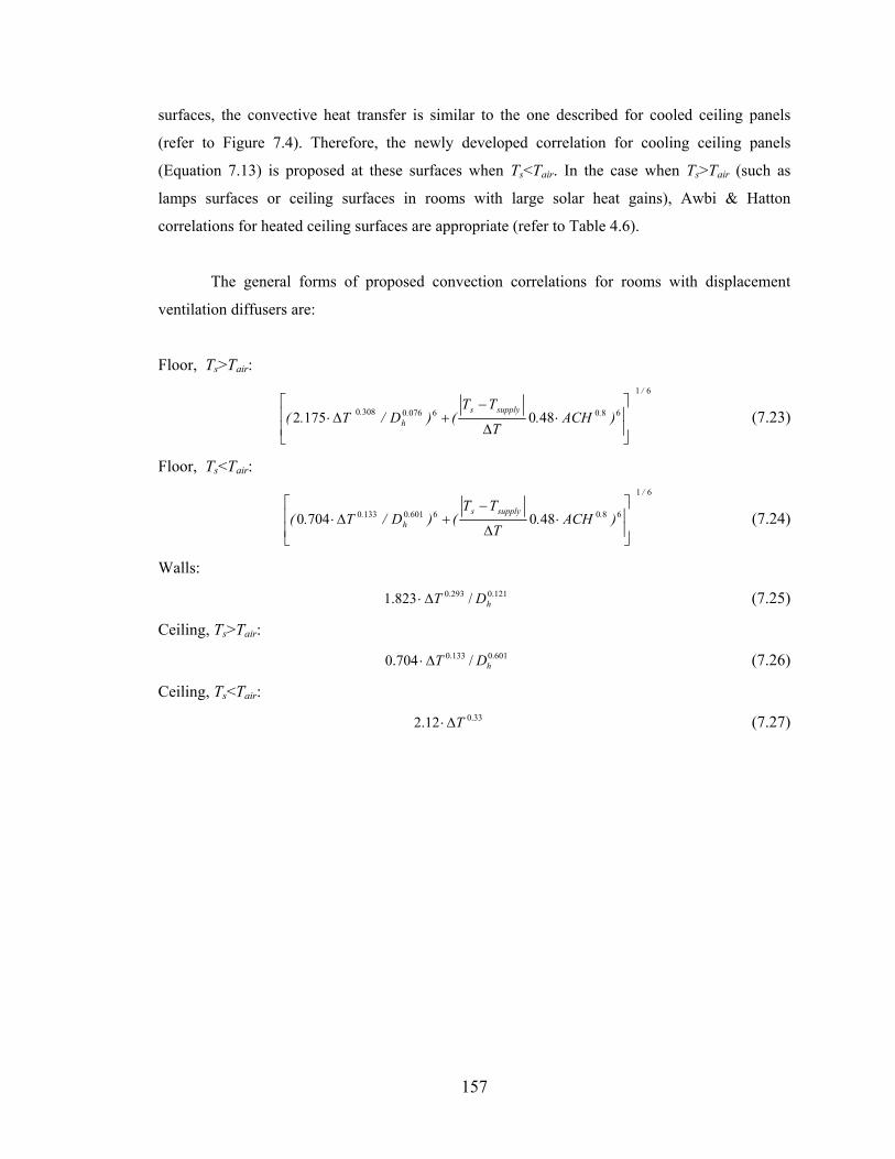
157

surfaces, the convective heat transfer is similar to the one described for cooled ceiling panels

(refer to Figure 7.4). Therefore, the newly developed correlation for cooling ceiling panels

(Equation 7.13) is proposed at these surfaces when Ts<Tair. In the case when Ts>Tair (such as

lamps surfaces or ceiling surfaces in rooms with large solar heat gains), Awbi & Hatton

correlations for heated ceiling surfaces are appropriate (refer to Table 4.6).

The general forms of proposed convection correlations for rooms with displacement

ventilation diffusers are:

Floor, Ts>Tair: 61

680607603080 4801752

/

.supplys.h

. )ACH.T

TT()D/T.(

⋅

∆

−+∆⋅ (7.23)

Floor, Ts<Tair: 61

680660101330 4807040

/

.supplys.h

. )ACH.T

TT()D/T.(

⋅

∆

−+∆⋅ (7.24)

Walls: 121.0293.0 /823.1 hDT∆⋅ (7.25)

Ceiling, Ts>Tair: 601.0133.0 /704.0 hDT∆⋅ (7.26)

Ceiling, Ts<Tair: 33.012.2 T∆⋅ (7.27)

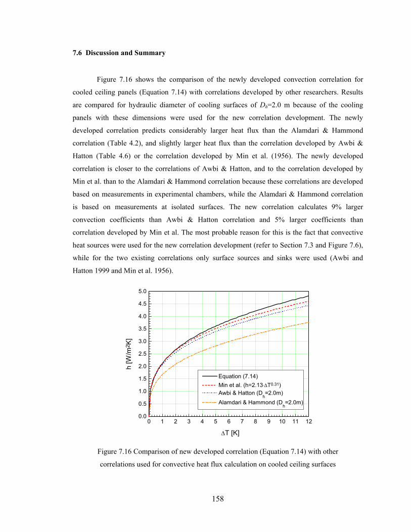
158

7.6 Discussion and Summary

Figure 7.16 shows the comparison of the newly developed convection correlation for

cooled ceiling panels (Equation 7.14) with correlations developed by other researchers. Results

are compared for hydraulic diameter of cooling surfaces of Dh=2.0 m because of the cooling

panels with these dimensions were used for the new correlation development. The newly

developed correlation predicts considerably larger heat flux than the Alamdari & Hammond

correlation (Table 4.2), and slightly larger heat flux than the correlation developed by Awbi &

Hatton (Table 4.6) or the correlation developed by Min et al. (1956). The newly developed

correlation is closer to the correlations of Awbi & Hatton, and to the correlation developed by

Min et al. than to the Alamdari & Hammond correlation because these correlations are developed

based on measurements in experimental chambers, while the Alamdari & Hammond correlation

is based on measurements at isolated surfaces. The new correlation calculates 9% larger

convection coefficients than Awbi & Hatton correlation and 5% larger coefficients than

correlation developed by Min et al. The most probable reason for this is the fact that convective

heat sources were used for the new correlation development (refer to Section 7.3 and Figure 7.6),

while for the two existing correlations only surface sources and sinks were used (Awbi and

Hatton 1999 and Min et al. 1956).

0 1 2 3 4 5 6 7 8 9 10 11 120.0

0.5

1.0

1.5

2.0

2.5

3.0

3.5

4.0

4.5

5.0

h [W

/m2 K

]

∆T [K]

Equation (7.14) Min et al. (h=2.13.∆T0.31) Awbi & Hatton (D

h=2.0m)

Alamdari & Hammond (Dh=2.0m)

Figure 7.16 Comparison of new developed correlation (Equation 7.14) with other

correlations used for convective heat flux calculation on cooled ceiling surfaces

159

Convection correlations for high aspiration diffusers (Equations 7.16-7.20) were

developed for the use in rooms when these diffusers are combined with radiant cooling panels.

These rooms have low ACH because only fresh air is supplied and the effect of supply

temperature on local air temperatures in the vicinity of the surfaces is small. Therefore, these

correlations are based on local temperatures. In the cases when high aspiration diffusers are used

with all air systems and a considerably larger supply air flow rate, the effect of supply

temperature is not negligible. In these rooms, the new convection correlations (7.16-7.20) should

not be used because they neglect the effect of supply temperature on the surface heat transfer.

Also, these correlations are valid for volume flow rates that provide less than 5 ACH in the room.

During the development of the new convection correlations, special attention was

dedicated to development of a convection correlation for floor surfaces in rooms with

displacement ventilation. Precise calculation of convective heat flux at floor surfaces in room

with DV is crucial for room temperature profile calculation (Yuan 1998). Heat flux at these

surfaces depends on supply air temperature, volume flow rate, and local air temperature.

Therefore, new convection correlations (7.23 and 7.24) have a general form, which combines the

effects of local temperature (surface and local air temperature difference) and air supply

temperature (surface and supply temperature difference).

Considering effects of a high aspiration diffuser on convection at a cooled ceiling, the

general equation (7.19) for combined natural and forced convection at cooled ceiling surfaces

shows that the effect of forced convection with high aspiration diffusers is not negligible. This is

especially the case for large flow rates. For example, for ∆T=8°C and a volume flow rate that

provides 4 ACH, the increase of the convection coefficient is 18%.

The newly developed convection correlations presented in this chapter were implemented

into MACA in order to improve the accuracy of thermal boundary conditions calculations in a

CFD simulation domain. Moreover, the use of these correlations is not limited to CFD-type

simulations. For example, the correlations for cooled ceiling combined with high aspiration

diffuser, Equations (7.16-7.20), can also be used in ES programs or in standard design procedures

by assuming perfect mixing (Troom=Tlocal air). Also, Equation (7.21) for the forced convection

correlation at a floor with displacement ventilation can be applied in ES or in standard design

procedures because it uses supply air temperature as the reference temperature and does not need

air temperature distribution.

160

CHAPTER 8

LABORATORY MEASUREMENTS AND RESULT ANALYSIS

8.1 Introduction

In this thesis, measurements were conducted in a controlled laboratory environment for

the following three different purposes:

1) collecting data for development of surface convection correlations,

2) collecting data for validation of new model for thermal boundary conditions in CFD,

3) collecting data for evaluation of CFD models used for air quality and thermal comfort

studies.

All these measurements were conducted in The Building Energy and Environmental

Systems Testing Facility at the Architectural Engineering department of Penn State University.

Activities related to measurements in this facility include not only work on setting-up the

experiments and data collection, but also work on design and construction of this facility. In the

next section of this chapter (Section 8.2), the experimental facility is described. Sections 8.3, 8.4,

and 8.5 provide the experimental set-up and the results for each of the three types of above

mentioned measurements. In Section 8.6, an analysis of measurement uncertainty is provided.

Finally, Section 8.7 provides a short summary of this chapter.

8.2 Experimental Facility

The Building Energy and Environmental Systems Testing Facility is a state-of-the-art

installation designed for full-scale thermal and air quality research. The facility consists of

environmental and climate chambers with two separate Heating Ventilating and Air-Conditioning

(HVAC) systems (Figure 8.1). An important part of this facility is the sophisticated measuring

and data acquisition system used for measurements of: energy, air, and tracer gas concentration in

different components of this facility.

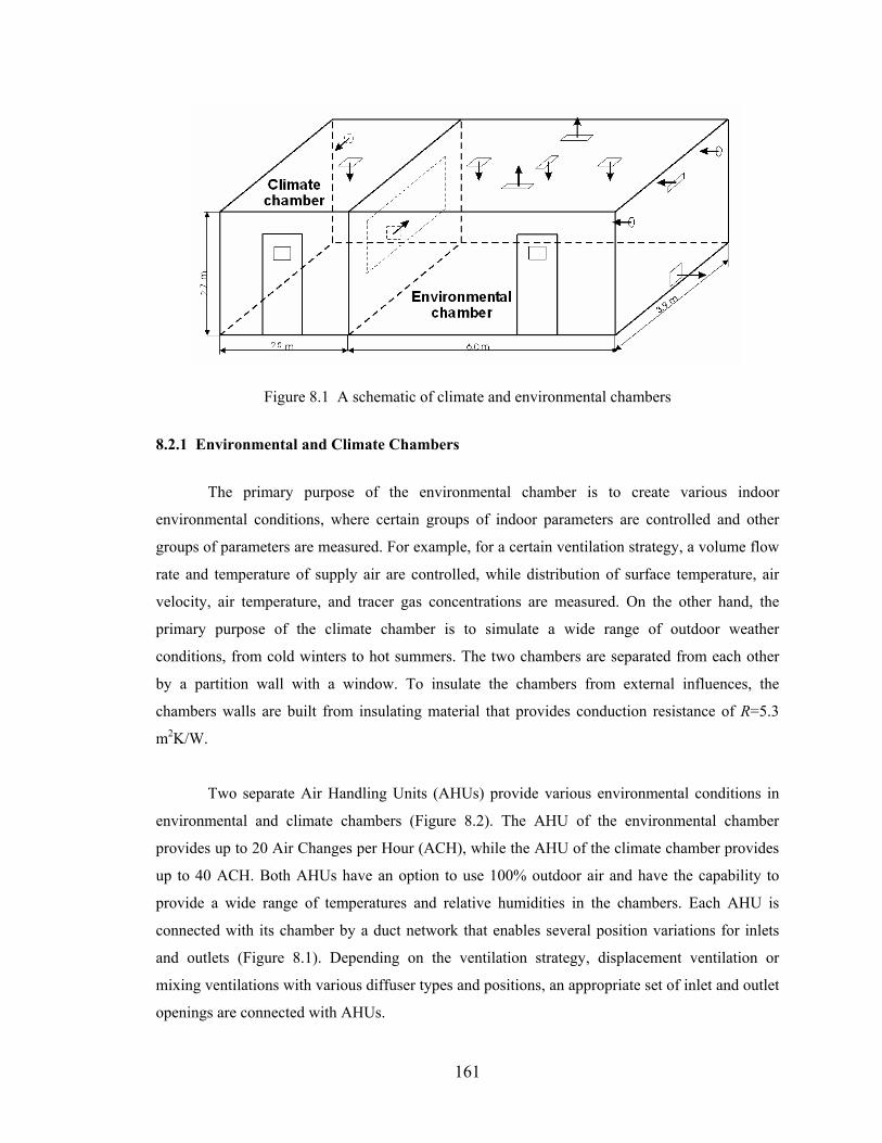
161

Figure 8.1 A schematic of climate and environmental chambers

8.2.1 Environmental and Climate Chambers

The primary purpose of the environmental chamber is to create various indoor

environmental conditions, where certain groups of indoor parameters are controlled and other

groups of parameters are measured. For example, for a certain ventilation strategy, a volume flow

rate and temperature of supply air are controlled, while distribution of surface temperature, air

velocity, air temperature, and tracer gas concentrations are measured. On the other hand, the

primary purpose of the climate chamber is to simulate a wide range of outdoor weather

conditions, from cold winters to hot summers. The two chambers are separated from each other

by a partition wall with a window. To insulate the chambers from external influences, the

chambers walls are built from insulating material that provides conduction resistance of R=5.3

m2K/W.

Two separate Air Handling Units (AHUs) provide various environmental conditions in

environmental and climate chambers (Figure 8.2). The AHU of the environmental chamber

provides up to 20 Air Changes per Hour (ACH), while the AHU of the climate chamber provides

up to 40 ACH. Both AHUs have an option to use 100% outdoor air and have the capability to

provide a wide range of temperatures and relative humidities in the chambers. Each AHU is

connected with its chamber by a duct network that enables several position variations for inlets

and outlets (Figure 8.1). Depending on the ventilation strategy, displacement ventilation or

mixing ventilations with various diffuser types and positions, an appropriate set of inlet and outlet

openings are connected with AHUs.

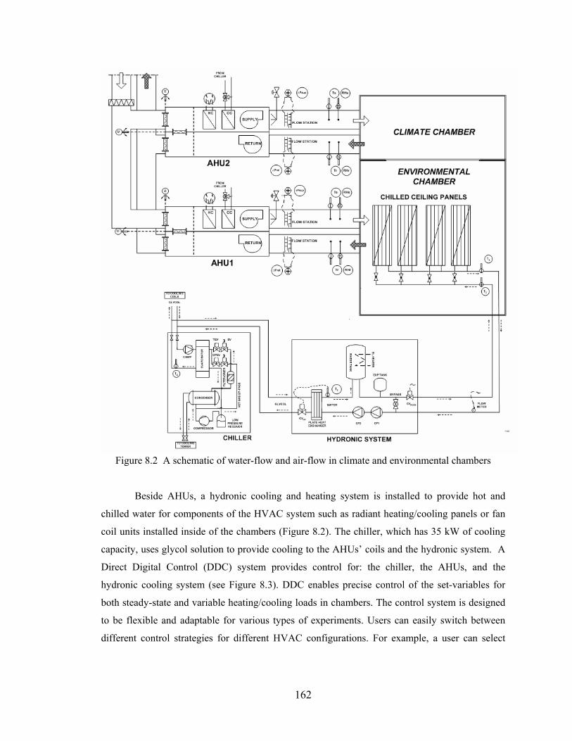
162

Figure 8.2 A schematic of water-flow and air-flow in climate and environmental chambers

Beside AHUs, a hydronic cooling and heating system is installed to provide hot and

chilled water for components of the HVAC system such as radiant heating/cooling panels or fan

coil units installed inside of the chambers (Figure 8.2). The chiller, which has 35 kW of cooling

capacity, uses glycol solution to provide cooling to the AHUs’ coils and the hydronic system. A

Direct Digital Control (DDC) system provides control for: the chiller, the AHUs, and the

hydronic cooling system (see Figure 8.3). DDC enables precise control of the set-variables for

both steady-state and variable heating/cooling loads in chambers. The control system is designed

to be flexible and adaptable for various types of experiments. Users can easily switch between

different control strategies for different HVAC configurations. For example, a user can select

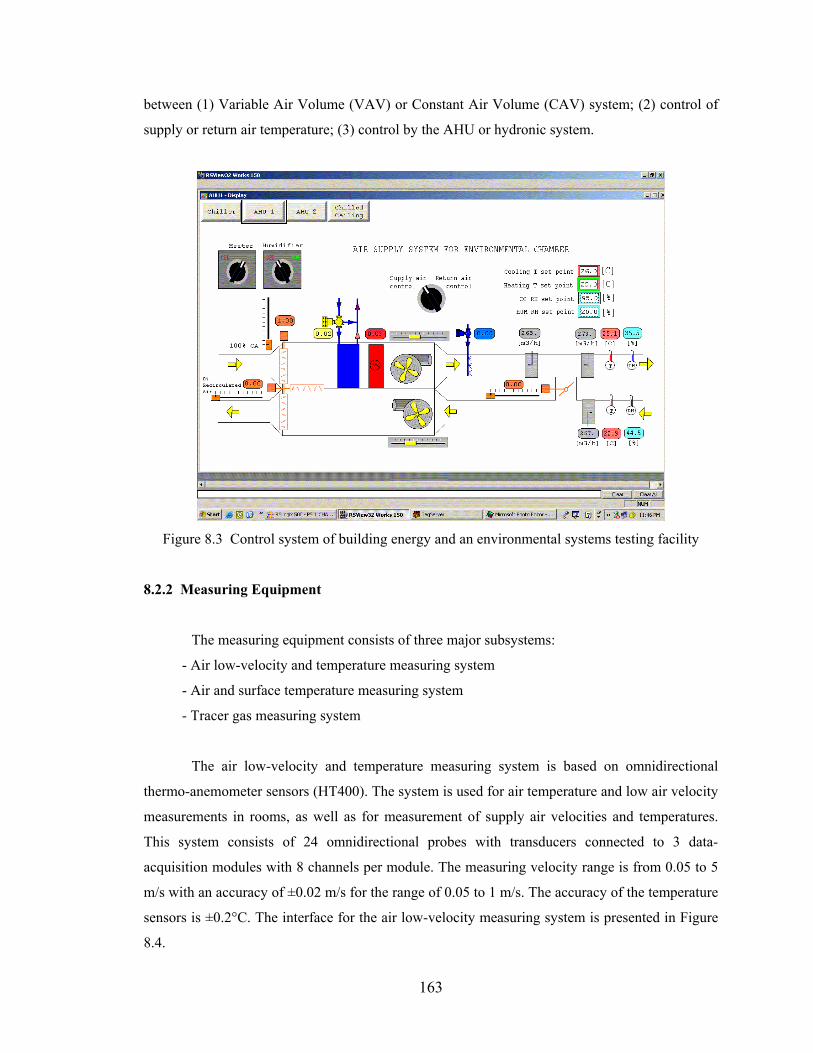
163

between (1) Variable Air Volume (VAV) or Constant Air Volume (CAV) system; (2) control of

supply or return air temperature; (3) control by the AHU or hydronic system.

Figure 8.3 Control system of building energy and an environmental systems testing facility

8.2.2 Measuring Equipment

The measuring equipment consists of three major subsystems:

- Air low-velocity and temperature measuring system

- Air and surface temperature measuring system

- Tracer gas measuring system

The air low-velocity and temperature measuring system is based on omnidirectional

thermo-anemometer sensors (HT400). The system is used for air temperature and low air velocity

measurements in rooms, as well as for measurement of supply air velocities and temperatures.

This system consists of 24 omnidirectional probes with transducers connected to 3 data-

acquisition modules with 8 channels per module. The measuring velocity range is from 0.05 to 5

m/s with an accuracy of ±0.02 m/s for the range of 0.05 to 1 m/s. The accuracy of the temperature

sensors is ±0.2°C. The interface for the air low-velocity measuring system is presented in Figure

8.4.

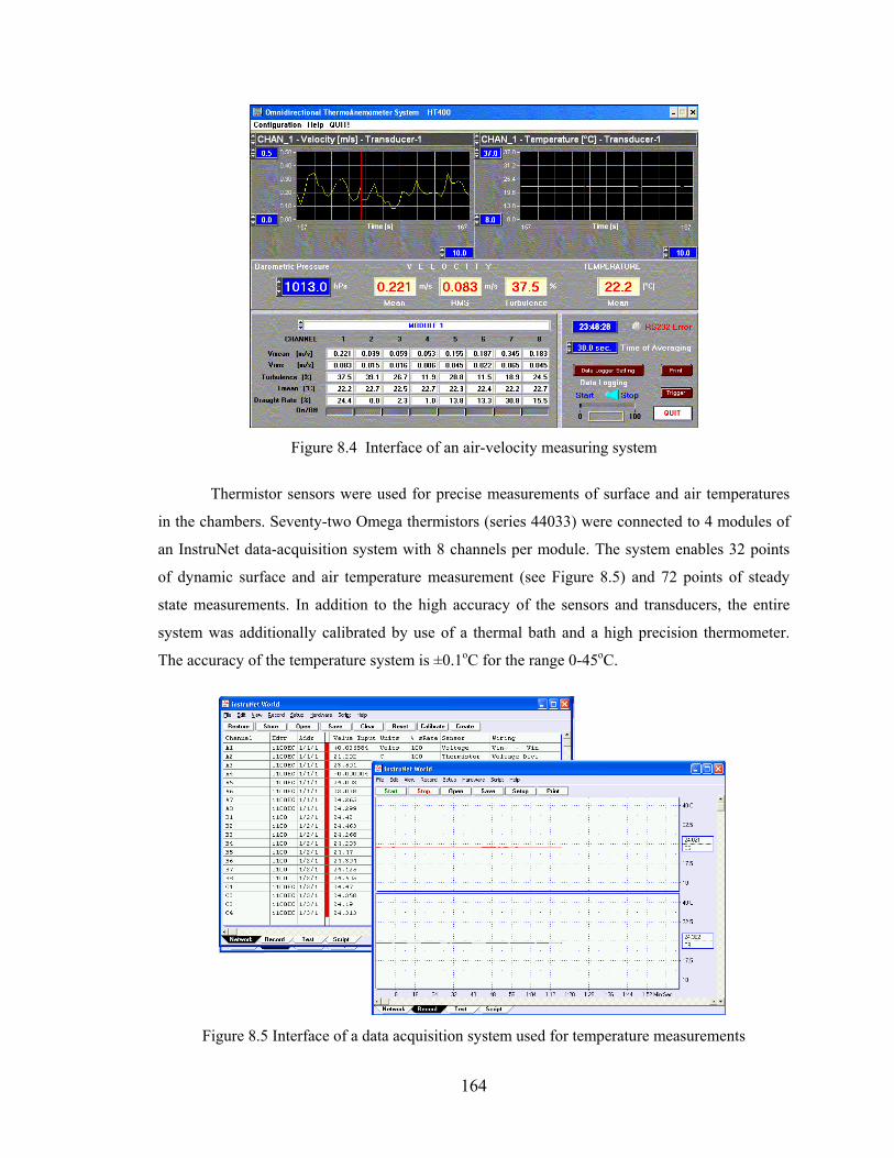
164

Figure 8.4 Interface of an air-velocity measuring system

Thermistor sensors were used for precise measurements of surface and air temperatures

in the chambers. Seventy-two Omega thermistors (series 44033) were connected to 4 modules of

an InstruNet data-acquisition system with 8 channels per module. The system enables 32 points

of dynamic surface and air temperature measurement (see Figure 8.5) and 72 points of steady

state measurements. In addition to the high accuracy of the sensors and transducers, the entire

system was additionally calibrated by use of a thermal bath and a high precision thermometer.

The accuracy of the temperature system is ±0.1oC for the range 0-45oC.

Figure 8.5 Interface of a data acquisition system used for temperature measurements

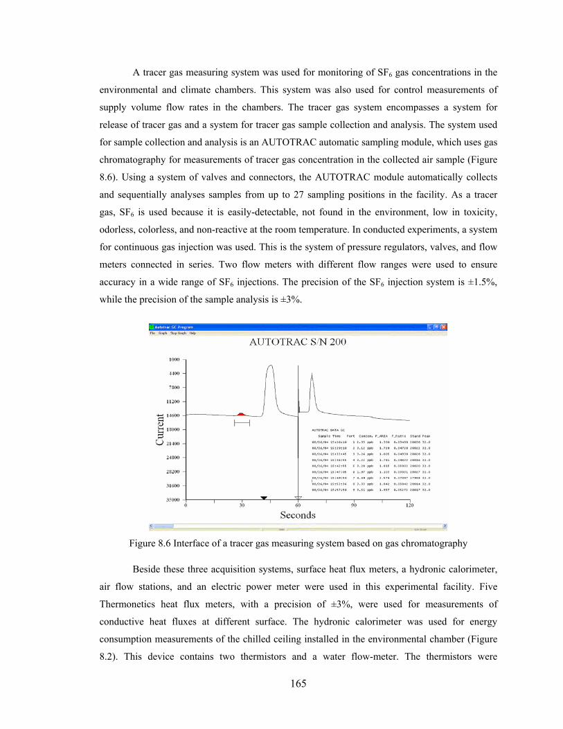
165

A tracer gas measuring system was used for monitoring of SF6 gas concentrations in the

environmental and climate chambers. This system was also used for control measurements of

supply volume flow rates in the chambers. The tracer gas system encompasses a system for

release of tracer gas and a system for tracer gas sample collection and analysis. The system used

for sample collection and analysis is an AUTOTRAC automatic sampling module, which uses gas

chromatography for measurements of tracer gas concentration in the collected air sample (Figure

8.6). Using a system of valves and connectors, the AUTOTRAC module automatically collects

and sequentially analyses samples from up to 27 sampling positions in the facility. As a tracer

gas, SF6 is used because it is easily-detectable, not found in the environment, low in toxicity,

odorless, colorless, and non-reactive at the room temperature. In conducted experiments, a system

for continuous gas injection was used. This is the system of pressure regulators, valves, and flow

meters connected in series. Two flow meters with different flow ranges were used to ensure

accuracy in a wide range of SF6 injections. The precision of the SF6 injection system is ±1.5%,

while the precision of the sample analysis is ±3%.

Figure 8.6 Interface of a tracer gas measuring system based on gas chromatography

Beside these three acquisition systems, surface heat flux meters, a hydronic calorimeter,

air flow stations, and an electric power meter were used in this experimental facility. Five

Thermonetics heat flux meters, with a precision of ±3%, were used for measurements of

conductive heat fluxes at different surface. The hydronic calorimeter was used for energy

consumption measurements of the chilled ceiling installed in the environmental chamber (Figure

8.2). This device contains two thermistors and a water flow-meter. The thermistors were

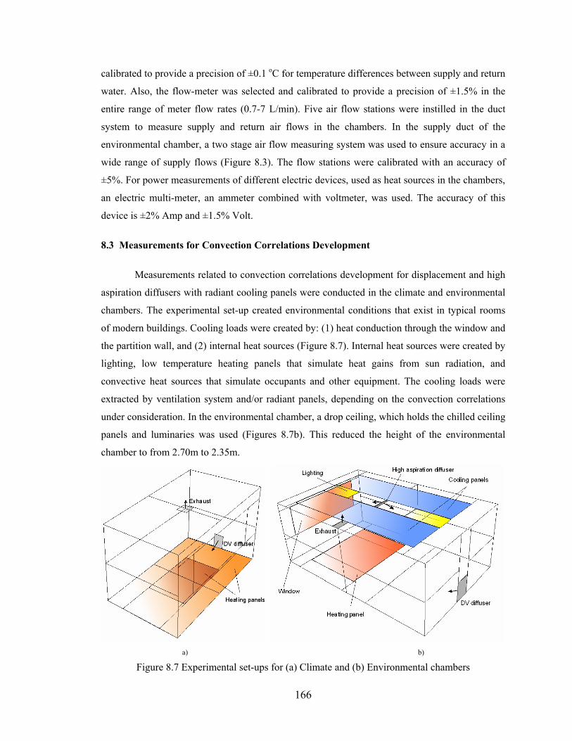
166

calibrated to provide a precision of ±0.1 oC for temperature differences between supply and return

water. Also, the flow-meter was selected and calibrated to provide a precision of ±1.5% in the

entire range of meter flow rates (0.7-7 L/min). Five air flow stations were instilled in the duct

system to measure supply and return air flows in the chambers. In the supply duct of the

environmental chamber, a two stage air flow measuring system was used to ensure accuracy in a

wide range of supply flows (Figure 8.3). The flow stations were calibrated with an accuracy of

±5%. For power measurements of different electric devices, used as heat sources in the chambers,

an electric multi-meter, an ammeter combined with voltmeter, was used. The accuracy of this

device is ±2% Amp and ±1.5% Volt.

8.3 Measurements for Convection Correlations Development

Measurements related to convection correlations development for displacement and high

aspiration diffusers with radiant cooling panels were conducted in the climate and environmental

chambers. The experimental set-up created environmental conditions that exist in typical rooms

of modern buildings. Cooling loads were created by: (1) heat conduction through the window and

the partition wall, and (2) internal heat sources (Figure 8.7). Internal heat sources were created by

lighting, low temperature heating panels that simulate heat gains from sun radiation, and

convective heat sources that simulate occupants and other equipment. The cooling loads were

extracted by ventilation system and/or radiant panels, depending on the convection correlations

under consideration. In the environmental chamber, a drop ceiling, which holds the chilled ceiling

panels and luminaries was used (Figures 8.7b). This reduced the height of the environmental

chamber to from 2.70m to 2.35m.

a) b)

Figure 8.7 Experimental set-ups for (a) Climate and (b) Environmental chambers

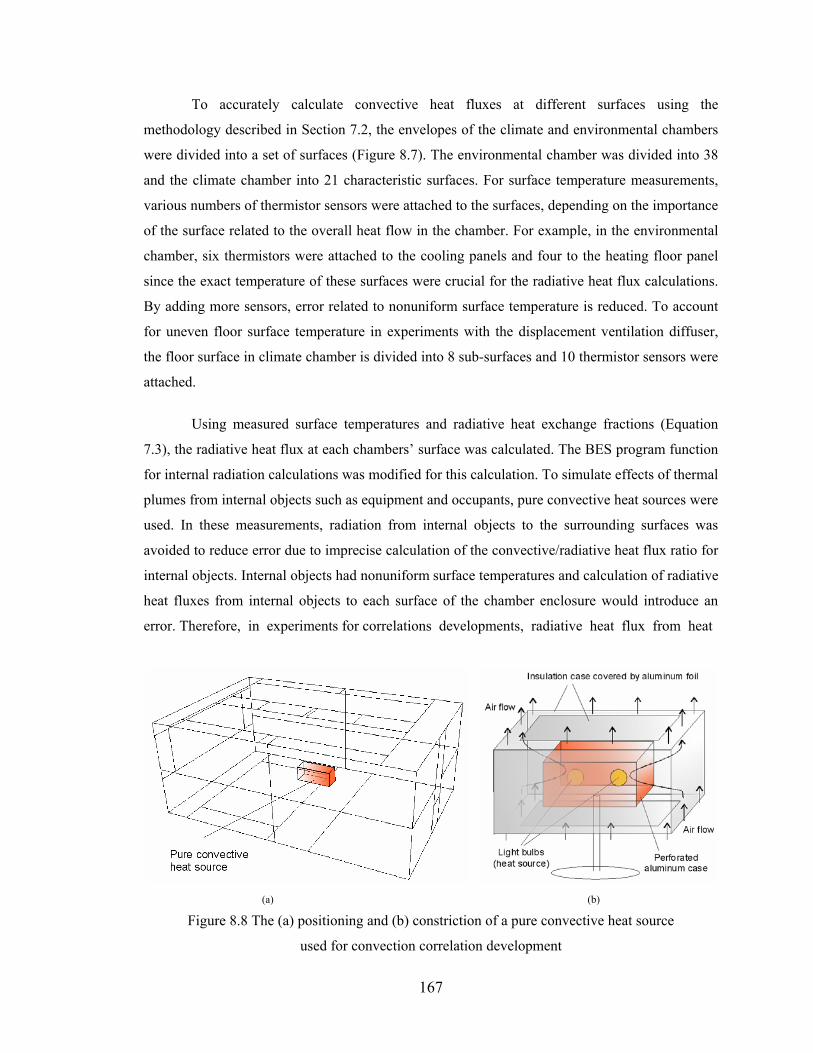
167

To accurately calculate convective heat fluxes at different surfaces using the

methodology described in Section 7.2, the envelopes of the climate and environmental chambers

were divided into a set of surfaces (Figure 8.7). The environmental chamber was divided into 38

and the climate chamber into 21 characteristic surfaces. For surface temperature measurements,

various numbers of thermistor sensors were attached to the surfaces, depending on the importance

of the surface related to the overall heat flow in the chamber. For example, in the environmental

chamber, six thermistors were attached to the cooling panels and four to the heating floor panel

since the exact temperature of these surfaces were crucial for the radiative heat flux calculations.

By adding more sensors, error related to nonuniform surface temperature is reduced. To account

for uneven floor surface temperature in experiments with the displacement ventilation diffuser,

the floor surface in climate chamber is divided into 8 sub-surfaces and 10 thermistor sensors were

attached.

Using measured surface temperatures and radiative heat exchange fractions (Equation

7.3), the radiative heat flux at each chambers’ surface was calculated. The BES program function

for internal radiation calculations was modified for this calculation. To simulate effects of thermal

plumes from internal objects such as equipment and occupants, pure convective heat sources were

used. In these measurements, radiation from internal objects to the surrounding surfaces was

avoided to reduce error due to imprecise calculation of the convective/radiative heat flux ratio for

internal objects. Internal objects had nonuniform surface temperatures and calculation of radiative

heat fluxes from internal objects to each surface of the chamber enclosure would introduce an

error. Therefore, in experiments for correlations developments, radiative heat flux from heat

(a) (b)

Figure 8.8 The (a) positioning and (b) constriction of a pure convective heat source

used for convection correlation development

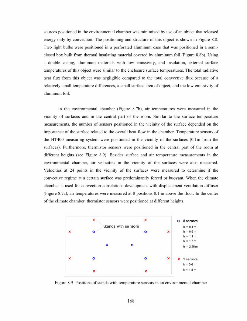
168

sources positioned in the environmental chamber was minimized by use of an object that released

energy only by convection. The positioning and structure of this object is shown in Figure 8.8.

Two light bulbs were positioned in a perforated aluminum case that was positioned in a semi-

closed box built from thermal insulating material covered by aluminum foil (Figure 8.8b). Using

a double casing, aluminum materials with low emissivity, and insulation, external surface

temperatures of this object were similar to the enclosure surface temperatures. The total radiative

heat flux from this object was negligible compared to the total convective flux because of a

relatively small temperature differences, a small surface area of object, and the low emissivity of

aluminum foil.

In the environmental chamber (Figure 8.7b), air temperatures were measured in the

vicinity of surfaces and in the central part of the room. Similar to the surface temperature

measurements, the number of sensors positioned in the vicinity of the surface depended on the

importance of the surface related to the overall heat flow in the chamber. Temperature sensors of

the HT400 measuring system were positioned in the vicinity of the surfaces (0.1m from the

surfaces). Furthermore, thermistor sensors were positioned in the central part of the room at

different heights (see Figure 8.9). Besides surface and air temperature measurements in the

environmental chamber, air velocities in the vicinity of the surfaces were also measured.

Velocities at 24 points in the vicinity of the surfaces were measured to determine if the

convective regime at a certain surface was predominantly forced or buoyant. When the climate

chamber is used for convection correlations development with displacement ventilation diffuser

(Figure 8.7a), air temperatures were measured at 8 positions 0.1 m above the floor. In the center

of the climate chamber, thermistor sensors were positioned at different heights.

5 sensors

2 sensors

5 sensors5 sensors

h = 0.1 m1

h = 0.6 m2

h = 1.1 m3

h = 1.7 m4

h = 2.25 m5

h = 0.6 m1

h = 1.8 m2

Stands with sensors

Figure 8.9 Positions of stands with temperature sensors in an environmental chamber

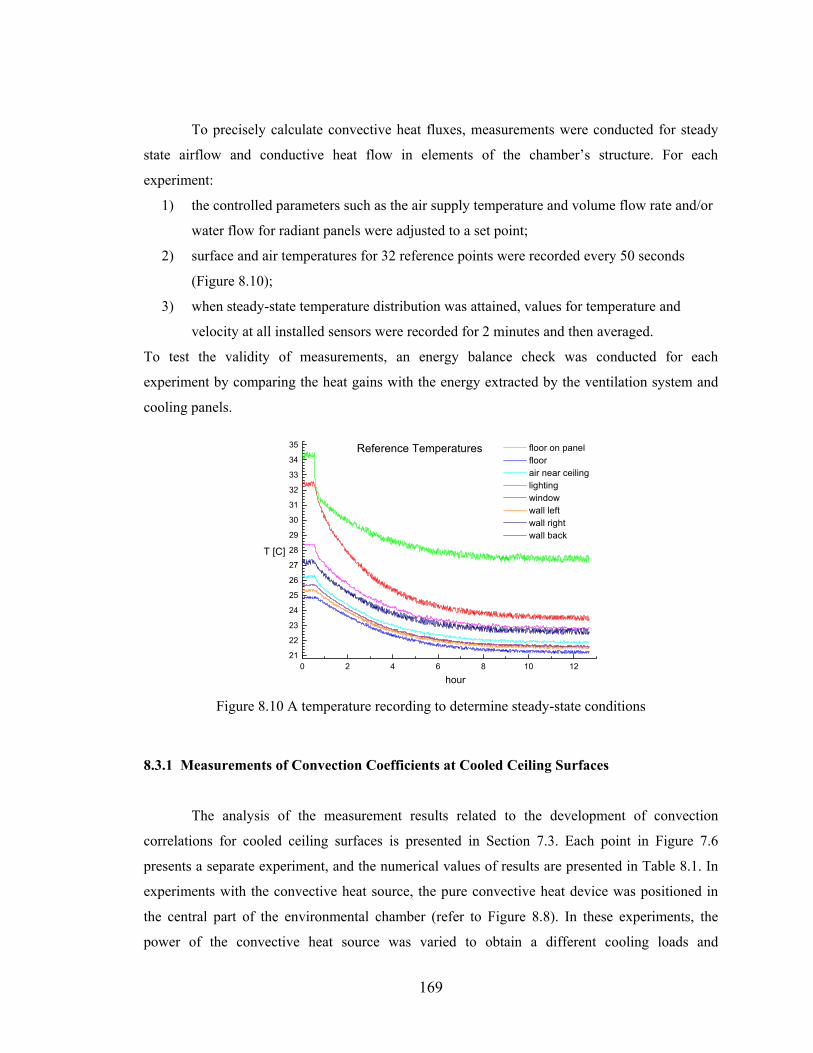
169

To precisely calculate convective heat fluxes, measurements were conducted for steady

state airflow and conductive heat flow in elements of the chamber’s structure. For each

experiment:

1) the controlled parameters such as the air supply temperature and volume flow rate and/or

water flow for radiant panels were adjusted to a set point;

2) surface and air temperatures for 32 reference points were recorded every 50 seconds

(Figure 8.10);

3) when steady-state temperature distribution was attained, values for temperature and

velocity at all installed sensors were recorded for 2 minutes and then averaged.

To test the validity of measurements, an energy balance check was conducted for each

experiment by comparing the heat gains with the energy extracted by the ventilation system and

cooling panels.

0 2 4 6 8 10 1221

22

23

24

25

26

27

28

29

30

31

32

33

34

35 Reference Temperatures floor on panel floor air near ceiling lighting window wall left wall right wall back

T [C]

hour Figure 8.10 A temperature recording to determine steady-state conditions

8.3.1 Measurements of Convection Coefficients at Cooled Ceiling Surfaces

The analysis of the measurement results related to the development of convection

correlations for cooled ceiling surfaces is presented in Section 7.3. Each point in Figure 7.6

presents a separate experiment, and the numerical values of results are presented in Table 8.1. In

experiments with the convective heat source, the pure convective heat device was positioned in

the central part of the environmental chamber (refer to Figure 8.8). In these experiments, the

power of the convective heat source was varied to obtain a different cooling loads and

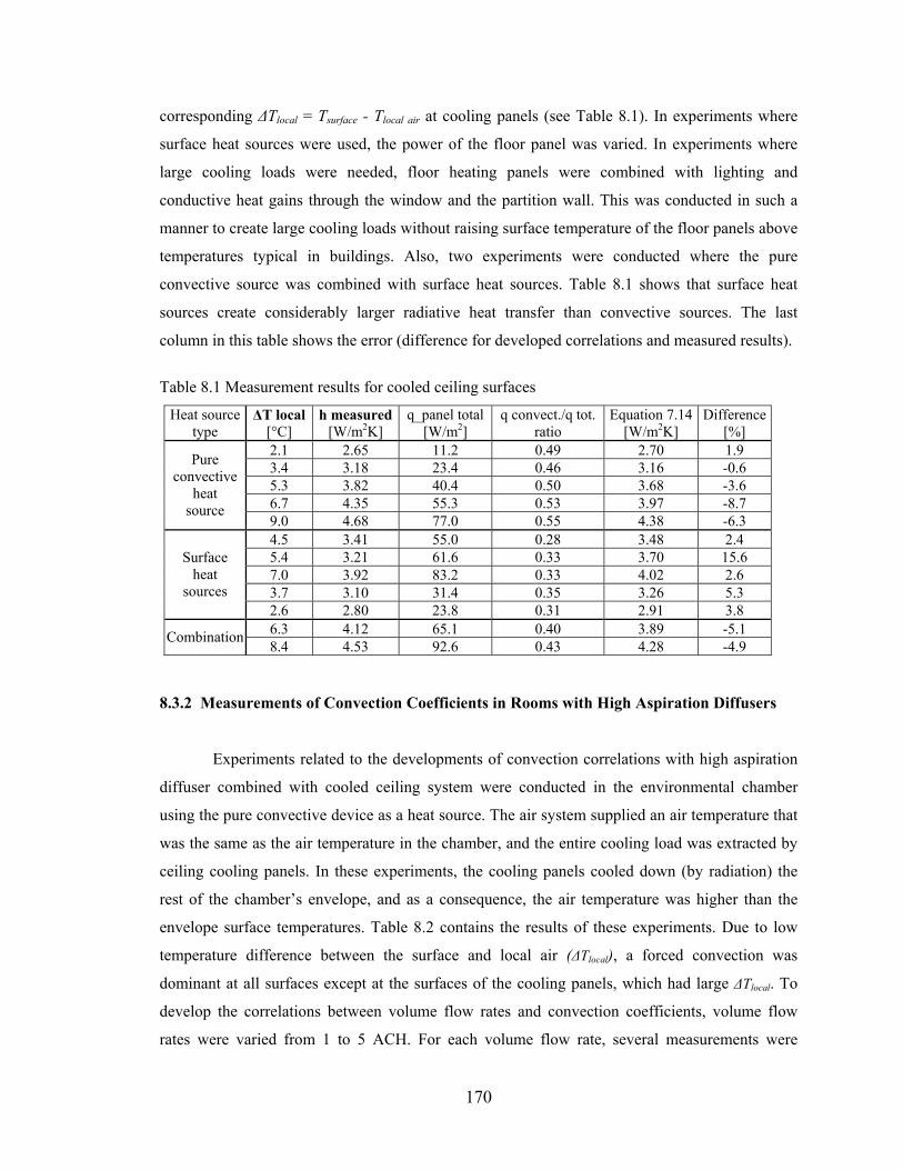
170

corresponding ∆Tlocal = Tsurface - Tlocal air at cooling panels (see Table 8.1). In experiments where

surface heat sources were used, the power of the floor panel was varied. In experiments where

large cooling loads were needed, floor heating panels were combined with lighting and

conductive heat gains through the window and the partition wall. This was conducted in such a

manner to create large cooling loads without raising surface temperature of the floor panels above

temperatures typical in buildings. Also, two experiments were conducted where the pure

convective source was combined with surface heat sources. Table 8.1 shows that surface heat

sources create considerably larger radiative heat transfer than convective sources. The last

column in this table shows the error (difference for developed correlations and measured results).

Table 8.1 Measurement results for cooled ceiling surfaces

Heat source type

∆T local [°C]

h measured[W/m2K]

q_panel total [W/m2]

q convect./q tot. ratio

Equation 7.14 [W/m2K]

Difference[%]

2.1 2.65 11.2 0.49 2.70 1.9 3.4 3.18 23.4 0.46 3.16 -0.6 5.3 3.82 40.4 0.50 3.68 -3.6 6.7 4.35 55.3 0.53 3.97 -8.7

Pure convective

heat source

9.0 4.68 77.0 0.55 4.38 -6.3 4.5 3.41 55.0 0.28 3.48 2.4 5.4 3.21 61.6 0.33 3.70 15.6 7.0 3.92 83.2 0.33 4.02 2.6 3.7 3.10 31.4 0.35 3.26 5.3

Surface heat

sources 2.6 2.80 23.8 0.31 2.91 3.8 6.3 4.12 65.1 0.40 3.89 -5.1 Combination 8.4 4.53 92.6 0.43 4.28 -4.9

8.3.2 Measurements of Convection Coefficients in Rooms with High Aspiration Diffusers

Experiments related to the developments of convection correlations with high aspiration

diffuser combined with cooled ceiling system were conducted in the environmental chamber

using the pure convective device as a heat source. The air system supplied an air temperature that

was the same as the air temperature in the chamber, and the entire cooling load was extracted by

ceiling cooling panels. In these experiments, the cooling panels cooled down (by radiation) the

rest of the chamber’s envelope, and as a consequence, the air temperature was higher than the

envelope surface temperatures. Table 8.2 contains the results of these experiments. Due to low

temperature difference between the surface and local air (∆Tlocal), a forced convection was

dominant at all surfaces except at the surfaces of the cooling panels, which had large ∆Tlocal. To

develop the correlations between volume flow rates and convection coefficients, volume flow

rates were varied from 1 to 5 ACH. For each volume flow rate, several measurements were

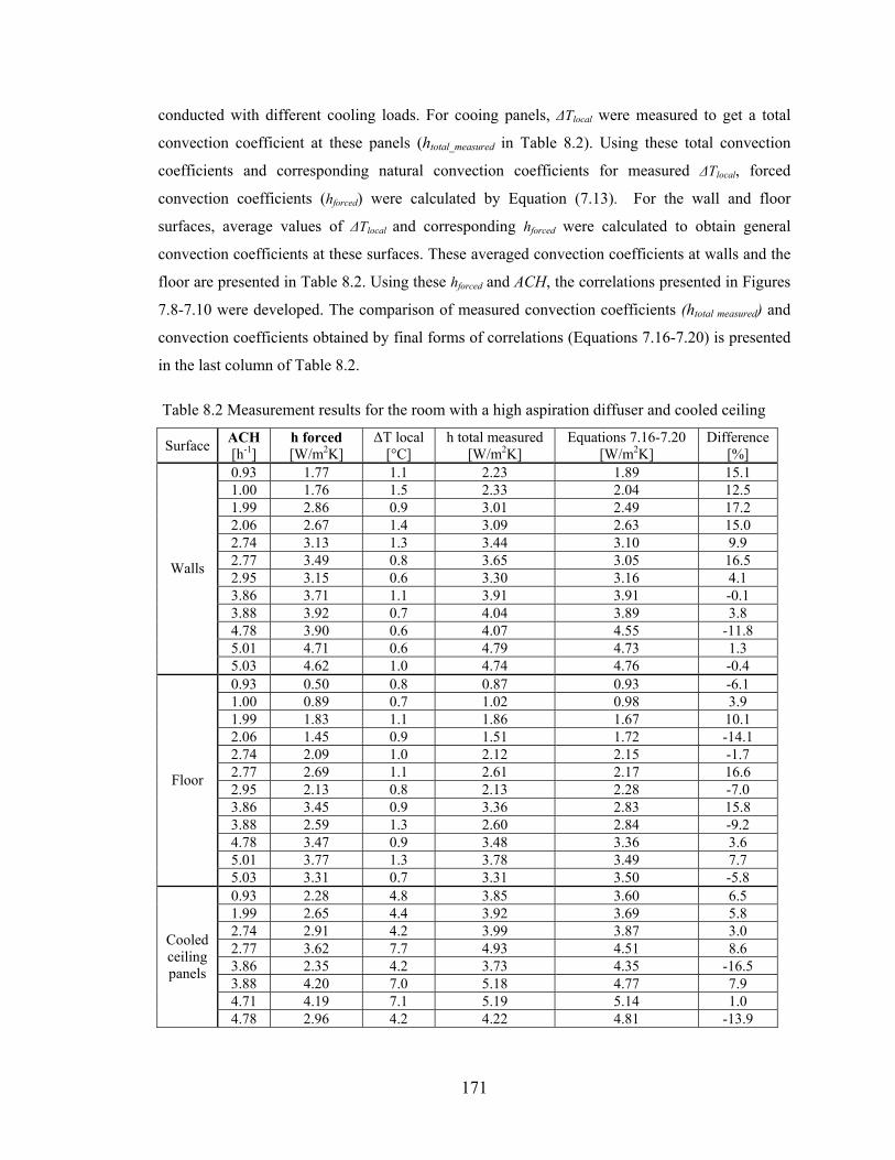
171

conducted with different cooling loads. For cooing panels, ∆Tlocal were measured to get a total

convection coefficient at these panels (htotal_measured in Table 8.2). Using these total convection

coefficients and corresponding natural convection coefficients for measured ∆Tlocal, forced

convection coefficients (hforced) were calculated by Equation (7.13). For the wall and floor

surfaces, average values of ∆Tlocal and corresponding hforced were calculated to obtain general

convection coefficients at these surfaces. These averaged convection coefficients at walls and the

floor are presented in Table 8.2. Using these hforced and ACH, the correlations presented in Figures

7.8-7.10 were developed. The comparison of measured convection coefficients (htotal measured) and

convection coefficients obtained by final forms of correlations (Equations 7.16-7.20) is presented

in the last column of Table 8.2. Table 8.2 Measurement results for the room with a high aspiration diffuser and cooled ceiling

Surface ACH [h-1]

h forced [W/m2K]

∆T local [°C]

h total measured [W/m2K]

Equations 7.16-7.20 [W/m2K]

Difference [%]

0.93 1.77 1.1 2.23 1.89 15.1 1.00 1.76 1.5 2.33 2.04 12.5 1.99 2.86 0.9 3.01 2.49 17.2 2.06 2.67 1.4 3.09 2.63 15.0 2.74 3.13 1.3 3.44 3.10 9.9 2.77 3.49 0.8 3.65 3.05 16.5 2.95 3.15 0.6 3.30 3.16 4.1 3.86 3.71 1.1 3.91 3.91 -0.1 3.88 3.92 0.7 4.04 3.89 3.8 4.78 3.90 0.6 4.07 4.55 -11.8 5.01 4.71 0.6 4.79 4.73 1.3

Walls

5.03 4.62 1.0 4.74 4.76 -0.4 0.93 0.50 0.8 0.87 0.93 -6.1 1.00 0.89 0.7 1.02 0.98 3.9 1.99 1.83 1.1 1.86 1.67 10.1 2.06 1.45 0.9 1.51 1.72 -14.1 2.74 2.09 1.0 2.12 2.15 -1.7 2.77 2.69 1.1 2.61 2.17 16.6 2.95 2.13 0.8 2.13 2.28 -7.0 3.86 3.45 0.9 3.36 2.83 15.8 3.88 2.59 1.3 2.60 2.84 -9.2 4.78 3.47 0.9 3.48 3.36 3.6 5.01 3.77 1.3 3.78 3.49 7.7

Floor

5.03 3.31 0.7 3.31 3.50 -5.8 0.93 2.28 4.8 3.85 3.60 6.5 1.99 2.65 4.4 3.92 3.69 5.8 2.74 2.91 4.2 3.99 3.87 3.0 2.77 3.62 7.7 4.93 4.51 8.6 3.86 2.35 4.2 3.73 4.35 -16.5 3.88 4.20 7.0 5.18 4.77 7.9 4.71 4.19 7.1 5.19 5.14 1.0

Cooled ceiling panels

4.78 2.96 4.2 4.22 4.81 -13.9

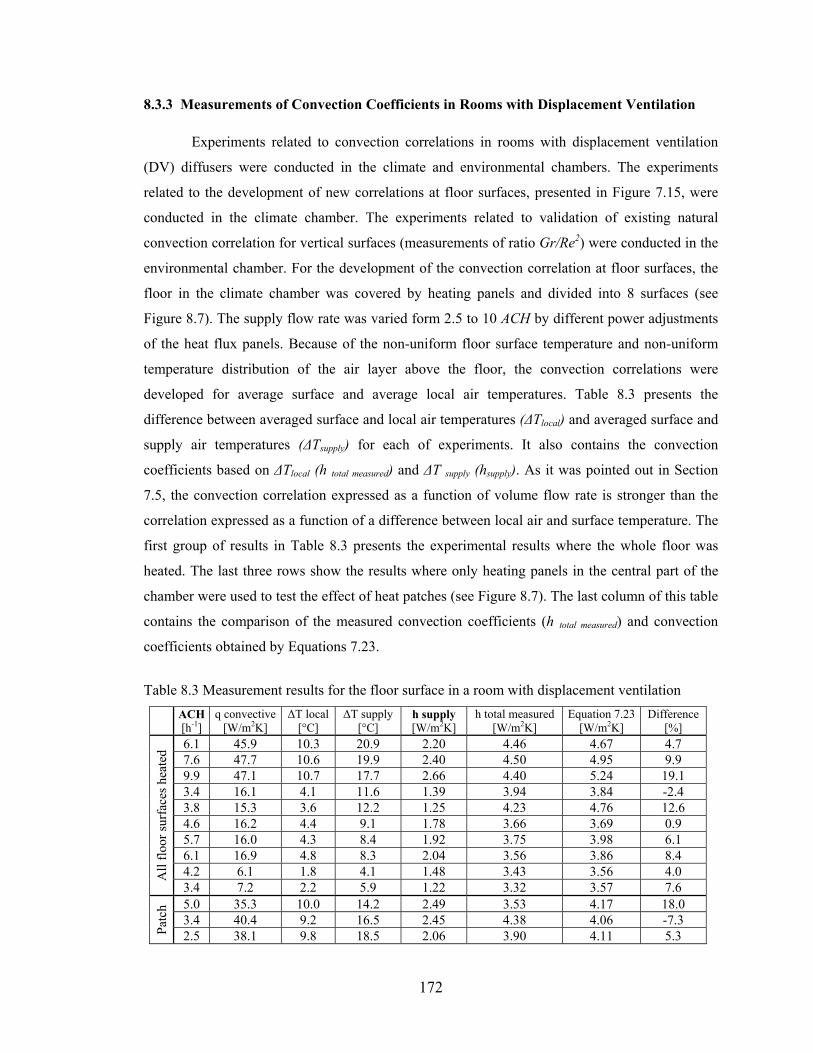
172

8.3.3 Measurements of Convection Coefficients in Rooms with Displacement Ventilation Experiments related to convection correlations in rooms with displacement ventilation

(DV) diffusers were conducted in the climate and environmental chambers. The experiments

related to the development of new correlations at floor surfaces, presented in Figure 7.15, were

conducted in the climate chamber. The experiments related to validation of existing natural

convection correlation for vertical surfaces (measurements of ratio Gr/Re2) were conducted in the

environmental chamber. For the development of the convection correlation at floor surfaces, the

floor in the climate chamber was covered by heating panels and divided into 8 surfaces (see

Figure 8.7). The supply flow rate was varied form 2.5 to 10 ACH by different power adjustments

of the heat flux panels. Because of the non-uniform floor surface temperature and non-uniform

temperature distribution of the air layer above the floor, the convection correlations were

developed for average surface and average local air temperatures. Table 8.3 presents the

difference between averaged surface and local air temperatures (∆Tlocal) and averaged surface and

supply air temperatures (∆Tsupply) for each of experiments. It also contains the convection

coefficients based on ∆Tlocal (h total measured) and ∆T supply (hsupply). As it was pointed out in Section

7.5, the convection correlation expressed as a function of volume flow rate is stronger than the

correlation expressed as a function of a difference between local air and surface temperature. The

first group of results in Table 8.3 presents the experimental results where the whole floor was

heated. The last three rows show the results where only heating panels in the central part of the

chamber were used to test the effect of heat patches (see Figure 8.7). The last column of this table

contains the comparison of the measured convection coefficients (h total measured) and convection

coefficients obtained by Equations 7.23.

Table 8.3 Measurement results for the floor surface in a room with displacement ventilation ACH

[h-1] q convective

[W/m2K] ∆T local

[°C] ∆T supply

[°C] h supply [W/m2K]

h total measured [W/m2K]

Equation 7.23 [W/m2K]

Difference [%]

6.1 45.9 10.3 20.9 2.20 4.46 4.67 4.7 7.6 47.7 10.6 19.9 2.40 4.50 4.95 9.9 9.9 47.1 10.7 17.7 2.66 4.40 5.24 19.1 3.4 16.1 4.1 11.6 1.39 3.94 3.84 -2.4 3.8 15.3 3.6 12.2 1.25 4.23 4.76 12.6 4.6 16.2 4.4 9.1 1.78 3.66 3.69 0.9 5.7 16.0 4.3 8.4 1.92 3.75 3.98 6.1 6.1 16.9 4.8 8.3 2.04 3.56 3.86 8.4 4.2 6.1 1.8 4.1 1.48 3.43 3.56 4.0 All

floor

surf

aces

hea

ted

3.4 7.2 2.2 5.9 1.22 3.32 3.57 7.6 5.0 35.3 10.0 14.2 2.49 3.53 4.17 18.0 3.4 40.4 9.2 16.5 2.45 4.38 4.06 -7.3

Patc

h

2.5 38.1 9.8 18.5 2.06 3.90 4.11 5.3

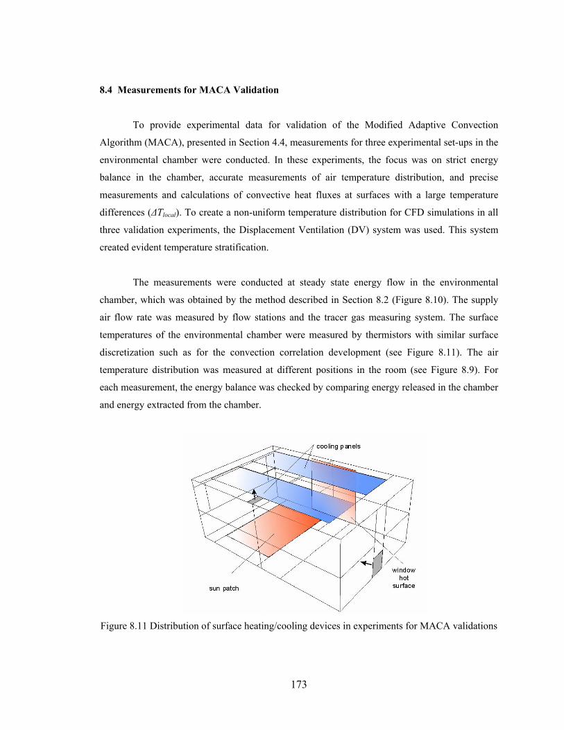
173

8.4 Measurements for MACA Validation

To provide experimental data for validation of the Modified Adaptive Convection

Algorithm (MACA), presented in Section 4.4, measurements for three experimental set-ups in the

environmental chamber were conducted. In these experiments, the focus was on strict energy

balance in the chamber, accurate measurements of air temperature distribution, and precise

measurements and calculations of convective heat fluxes at surfaces with a large temperature

differences (∆Tlocal). To create a non-uniform temperature distribution for CFD simulations in all

three validation experiments, the Displacement Ventilation (DV) system was used. This system

created evident temperature stratification.

The measurements were conducted at steady state energy flow in the environmental

chamber, which was obtained by the method described in Section 8.2 (Figure 8.10). The supply

air flow rate was measured by flow stations and the tracer gas measuring system. The surface

temperatures of the environmental chamber were measured by thermistors with similar surface

discretization such as for the convection correlation development (see Figure 8.11). The air

temperature distribution was measured at different positions in the room (see Figure 8.9). For

each measurement, the energy balance was checked by comparing energy released in the chamber

and energy extracted from the chamber.

Figure 8.11 Distribution of surface heating/cooling devices in experiments for MACA validations

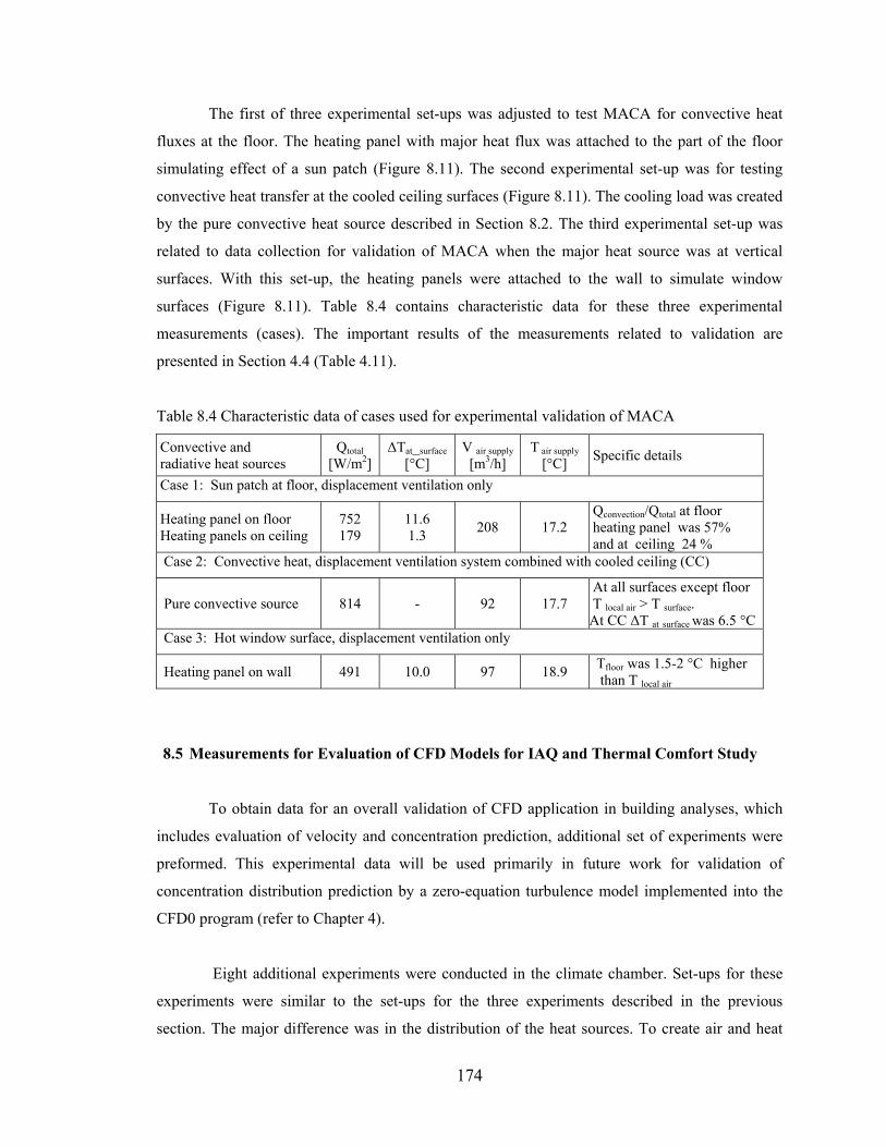
174

The first of three experimental set-ups was adjusted to test MACA for convective heat

fluxes at the floor. The heating panel with major heat flux was attached to the part of the floor

simulating effect of a sun patch (Figure 8.11). The second experimental set-up was for testing

convective heat transfer at the cooled ceiling surfaces (Figure 8.11). The cooling load was created

by the pure convective heat source described in Section 8.2. The third experimental set-up was

related to data collection for validation of MACA when the major heat source was at vertical

surfaces. With this set-up, the heating panels were attached to the wall to simulate window

surfaces (Figure 8.11). Table 8.4 contains characteristic data for these three experimental

measurements (cases). The important results of the measurements related to validation are

presented in Section 4.4 (Table 4.11).

Table 8.4 Characteristic data of cases used for experimental validation of MACA

Convective and radiative heat sources

Qtotal [W/m2]

∆Tat_surface [°C]

V air supply [m3/h]

T air supply [°C] Specific details

Case 1: Sun patch at floor, displacement ventilation only

Heating panel on floor Heating panels on ceiling

752 179

11.6 1.3 208 17.2

Qconvection/Qtotal at floor heating panel was 57% and at ceiling 24 %

Case 2: Convective heat, displacement ventilation system combined with cooled ceiling (CC)

Pure convective source 814 - 92 17.7 At all surfaces except floor T local air > T surface. At CC ∆T at surface was 6.5 °C

Case 3: Hot window surface, displacement ventilation only

Heating panel on wall 491 10.0 97 18.9 Tfloor was 1.5-2 °C higher than T local air

8.5 Measurements for Evaluation of CFD Models for IAQ and Thermal Comfort Study

To obtain data for an overall validation of CFD application in building analyses, which

includes evaluation of velocity and concentration prediction, additional set of experiments were

preformed. This experimental data will be used primarily in future work for validation of

concentration distribution prediction by a zero-equation turbulence model implemented into the

CFD0 program (refer to Chapter 4).

Eight additional experiments were conducted in the climate chamber. Set-ups for these

experiments were similar to the set-ups for the three experiments described in the previous

section. The major difference was in the distribution of the heat sources. To create air and heat

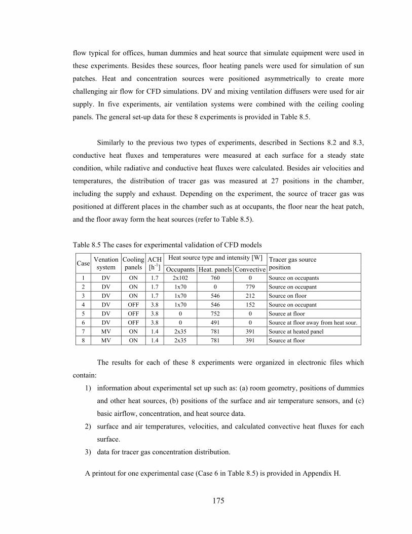
175

flow typical for offices, human dummies and heat source that simulate equipment were used in

these experiments. Besides these sources, floor heating panels were used for simulation of sun

patches. Heat and concentration sources were positioned asymmetrically to create more

challenging air flow for CFD simulations. DV and mixing ventilation diffusers were used for air

supply. In five experiments, air ventilation systems were combined with the ceiling cooling

panels. The general set-up data for these 8 experiments is provided in Table 8.5.

Similarly to the previous two types of experiments, described in Sections 8.2 and 8.3,

conductive heat fluxes and temperatures were measured at each surface for a steady state

condition, while radiative and conductive heat fluxes were calculated. Besides air velocities and

temperatures, the distribution of tracer gas was measured at 27 positions in the chamber,

including the supply and exhaust. Depending on the experiment, the source of tracer gas was

positioned at different places in the chamber such as at occupants, the floor near the heat patch,

and the floor away form the heat sources (refer to Table 8.5).

Table 8.5 The cases for experimental validation of CFD models

Heat source type and intensity [W] Case Venation

system Cooling panels

ACH [h-1] Occupants Heat. panels Convective

Tracer gas source position

1 DV ON 1.7 2x102 760 0 Source on occupants 2 DV ON 1.7 1x70 0 779 Source on occupant 3 DV ON 1.7 1x70 546 212 Source on floor 4 DV OFF 3.8 1x70 546 152 Source on occupant 5 DV OFF 3.8 0 752 0 Source at floor 6 DV OFF 3.8 0 491 0 Source at floor away from heat sour. 7 MV ON 1.4 2x35 781 391 Source at heated panel 8 MV ON 1.4 2x35 781 391 Source at floor

The results for each of these 8 experiments were organized in electronic files which

contain:

1) information about experimental set up such as: (a) room geometry, positions of dummies

and other heat sources, (b) positions of the surface and air temperature sensors, and (c)

basic airflow, concentration, and heat source data.

2) surface and air temperatures, velocities, and calculated convective heat fluxes for each

surface.

3) data for tracer gas concentration distribution.

A printout for one experimental case (Case 6 in Table 8.5) is provided in Appendix H.

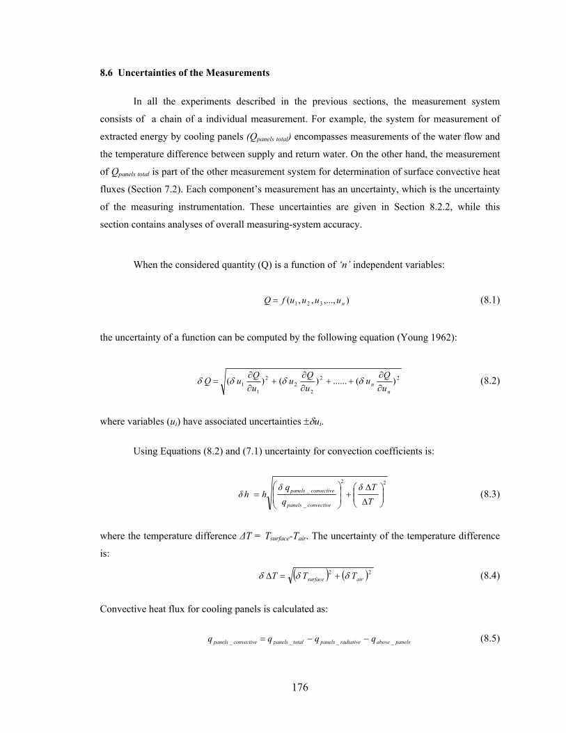
176

8.6 Uncertainties of the Measurements

In all the experiments described in the previous sections, the measurement system

consists of a chain of a individual measurement. For example, the system for measurement of

extracted energy by cooling panels (Qpanels total) encompasses measurements of the water flow and

the temperature difference between supply and return water. On the other hand, the measurement

of Qpanels total is part of the other measurement system for determination of surface convective heat

fluxes (Section 7.2). Each component’s measurement has an uncertainty, which is the uncertainty

of the measuring instrumentation. These uncertainties are given in Section 8.2.2, while this

section contains analyses of overall measuring-system accuracy.

When the considered quantity (Q) is a function of ‘n’ independent variables:

),...,,,( 321 nuuuufQ = (8.1)

the uncertainty of a function can be computed by the following equation (Young 1962):

22

22

2

11 )(......)()(

nn u

QuuQu

uQuQ

∂∂

++∂∂

+∂∂

= δδδδ (8.2)

where variables (ui) have associated uncertainties ±δui.

Using Equations (8.2) and (7.1) uncertainty for convection coefficients is:

22

_

_

∆

∆+

=

TTδ

qqδ

hh δconvectivepanels

convectivepanels (8.3)

where the temperature difference ∆T = Tsurface-Tair. The uncertainty of the temperature difference

is:

( ) ( )22airsurface TTT δδδ +=∆ (8.4)

Convective heat flux for cooling panels is calculated as:

panelsaboveradiativepanelstotalpanelsconvectivepanels qqqq ____ −−= (8.5)

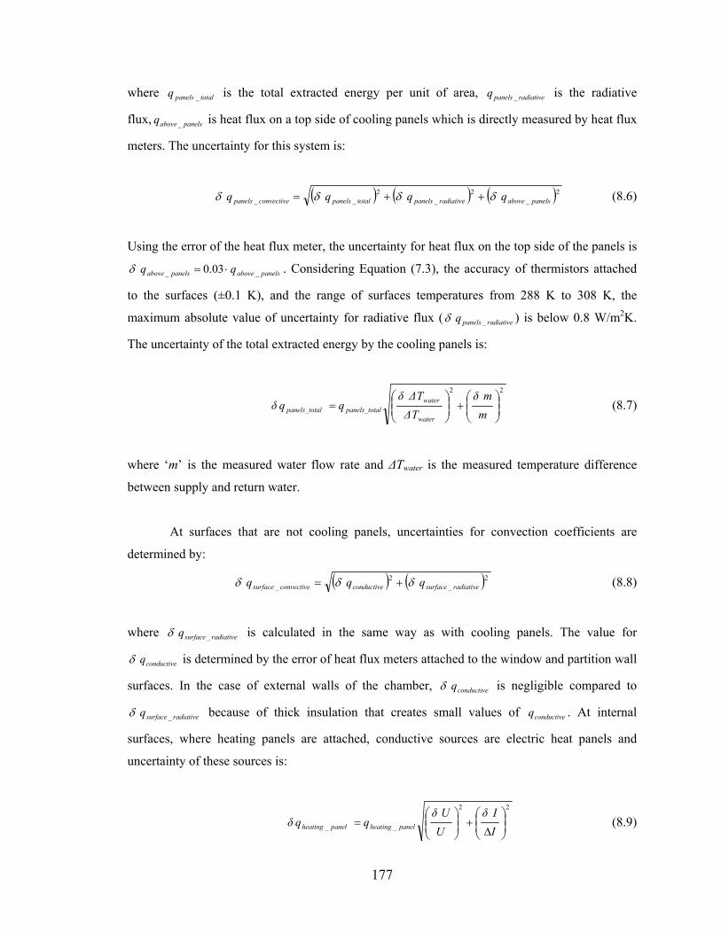
177

where totalpanelsq _ is the total extracted energy per unit of area, radiativepanelsq _ is the radiative

flux, panelsaboveq _ is heat flux on a top side of cooling panels which is directly measured by heat flux

meters. The uncertainty for this system is:

( ) ( ) ( )2_2

_2

__ panelsaboveradiativepanelstotalpanelsconvectivepanels qqqq δδδδ ++= (8.6)

Using the error of the heat flux meter, the uncertainty for heat flux on the top side of the panels is

panelsabovepanelsabove qq __ 03.0 ⋅=δ . Considering Equation (7.3), the accuracy of thermistors attached

to the surfaces (±0.1 K), and the range of surfaces temperatures from 288 K to 308 K, the

maximum absolute value of uncertainty for radiative flux ( radiativepanelsq _δ ) is below 0.8 W/m2K.

The uncertainty of the total extracted energy by the cooling panels is:

22

+

=

mmδ

T∆T∆δ

q qδwater

wateralpanels_totalpanels_tot (8.7)

where ‘m’ is the measured water flow rate and ∆Twater is the measured temperature difference

between supply and return water.

At surfaces that are not cooling panels, uncertainties for convection coefficients are

determined by:

( ) ( )2_2

_ radiativesurfaceconductiveconvectivesurface qqq δδδ += (8.8)

where radiativesurfaceq _δ is calculated in the same way as with cooling panels. The value for

conductiveqδ is determined by the error of heat flux meters attached to the window and partition wall

surfaces. In the case of external walls of the chamber, conductiveqδ is negligible compared to

radiativesurfaceq _δ because of thick insulation that creates small values of conductiveq . At internal

surfaces, where heating panels are attached, conductive sources are electric heat panels and

uncertainty of these sources is:

22

__

∆+

=

IIδ

UUδ

q qδ panelheatingpanelheating (8.9)

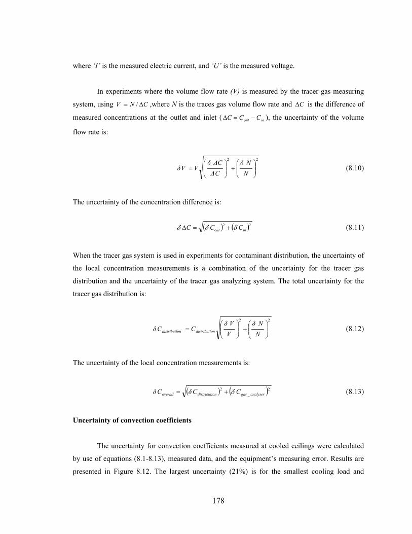
178

where ‘I’ is the measured electric current, and ‘U’ is the measured voltage.

In experiments where the volume flow rate (V) is measured by the tracer gas measuring

system, using CNV ∆= / ,where N is the traces gas volume flow rate and C∆ is the difference of

measured concentrations at the outlet and inlet ( inout CCC −=∆ ), the uncertainty of the volume

flow rate is:

22

+

=

NNδ

C∆∆Cδ

VV δ (8.10)

The uncertainty of the concentration difference is:

( ) ( )22

inout CCC δδδ +=∆ (8.11)

When the tracer gas system is used in experiments for contaminant distribution, the uncertainty of

the local concentration measurements is a combination of the uncertainty for the tracer gas

distribution and the uncertainty of the tracer gas analyzing system. The total uncertainty for the

tracer gas distribution is:

22

+

=

NNδ

VVδ

C Cδ ondistributiondistributi (8.12)

The uncertainty of the local concentration measurements is:

( ) ( )2_2

analysergasondistributioverall CCδCδ δ+= (8.13)

Uncertainty of convection coefficients

The uncertainty for convection coefficients measured at cooled ceilings were calculated

by use of equations (8.1-8.13), measured data, and the equipment’s measuring error. Results are

presented in Figure 8.12. The largest uncertainty (21%) is for the smallest cooling load and

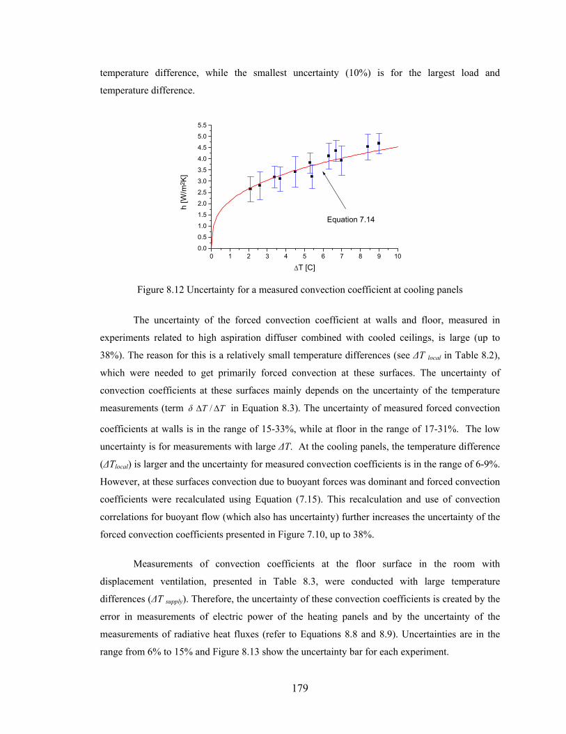
179

temperature difference, while the smallest uncertainty (10%) is for the largest load and

temperature difference.

0 1 2 3 4 5 6 7 8 9 100.0

0.5

1.0

1.5

2.0

2.5

3.0

3.5

4.0

4.5

5.0

5.5

Equation 7.14

h [W

/m2 K

]

∆T [C]

Figure 8.12 Uncertainty for a measured convection coefficient at cooling panels

The uncertainty of the forced convection coefficient at walls and floor, measured in

experiments related to high aspiration diffuser combined with cooled ceilings, is large (up to

38%). The reason for this is a relatively small temperature differences (see ∆T local in Table 8.2),

which were needed to get primarily forced convection at these surfaces. The uncertainty of

convection coefficients at these surfaces mainly depends on the uncertainty of the temperature

measurements (term TTδ ∆∆ / in Equation 8.3). The uncertainty of measured forced convection

coefficients at walls is in the range of 15-33%, while at floor in the range of 17-31%. The low

uncertainty is for measurements with large ∆T. At the cooling panels, the temperature difference

(∆Tlocal) is larger and the uncertainty for measured convection coefficients is in the range of 6-9%.

However, at these surfaces convection due to buoyant forces was dominant and forced convection

coefficients were recalculated using Equation (7.15). This recalculation and use of convection

correlations for buoyant flow (which also has uncertainty) further increases the uncertainty of the

forced convection coefficients presented in Figure 7.10, up to 38%.

Measurements of convection coefficients at the floor surface in the room with

displacement ventilation, presented in Table 8.3, were conducted with large temperature

differences (∆T supply). Therefore, the uncertainty of these convection coefficients is created by the

error in measurements of electric power of the heating panels and by the uncertainty of the

measurements of radiative heat fluxes (refer to Equations 8.8 and 8.9). Uncertainties are in the

range from 6% to 15% and Figure 8.13 show the uncertainty bar for each experiment.

180

0 1 2 3 4 5 6 7 8 9 10 110.0

0.5

1.0

1.5

2.0

2.5

3.0

3.5

Equation 7.21

h [W

/m2 K

]

ACH [hour-1] Figure 8.13 Uncertainty for a measured convection coefficient on floors in a room with

displacement ventilation diffuser

Uncertainty of data collected for validation of MACA

For validation of MACA, temperature and heat fluxes at all surfaces were measured to

calculate the overall heat transfer. However, in Section 4.4 experimental and simulation results

(heat fluxes) were compared primarily for surfaces which have a large temperature difference

(∆Tlocal) because this gives the smallest uncertainty in measurements. The uncertainties of

convective heat fluxes at the heating panels are 7% and 8% for experiment 1 and 3 respectively

(see Section 3). For experiment 2, the uncertainty of measured heat fluxes at the cooled ceiling

panel is 13%. The uncertainty of the supply airflow rate is 5%. The uncertainty of the temperature

measurements is ±0.2°C for air and ±0.1°C for surface temperatures.

Uncertainty of concentration distribution

In experiments related to concentration distribution, presented in Section 8.4, the tracer

gas concentrations were measured with an uncertainty of 7%, considering measuring equipment.

However, repeatability, defined as a difference of concentrations for two consecutive

measurements at the same point, was larger. The most probable reason for this is the imperfect

steady-state airflow, even when measured temperatures and total (ominidirectional) velocities

indicate steady state airflow. A small change in the velocity direction in the vicinity of the tracer

gas source may considerably affect the concentration distribution. The repeatability of

concentration measurements at locations in the room was in the range 5-14%, depending on the

type of airflow. The repeatability of measurements in supply and exhaust air was below 5%. The

uncertainty of temperature measurements is similar to the experiments related to the MACA

181

validation, while the uncertainty of convective heat fluxes at heating and cooling surfaces is in the

range of 7-15%. For other surfaces, the uncertainty is approximately equal to the uncertainty of

the radiative heat flux calculation (0.8 W/m2K).

Generally, the measurements presented in Sections 8.2-8.4 were conducted for an

experimental set-up that provided an environment similar to real buildings. As a consequence, the

ranges of environmental parameters such as the range of temperature differences, flow rates, and

velocities were relatively small. On the other hand, many parameters can be measured only by

measurements of several other parameters (components). Considering small velocities and

temperature differences and the complexity of experiments, the uncertainty of the conducted

measurements is relatively good for all measurements except for the forced convection

coefficients developed for use in the room with high aspiration diffuser.

The large uncertainty of forced convection coefficients with high aspiration diffusers (15-

38%) is difficult to avoid because a low temperature difference is needed to measure the heat

transfer caused by forced convection at room surfaces. However, these forced convection

correlations are developed primarily for correction of buoyant convection when high aspiration

diffuser is used with cooling panels (Equations 716-7.20). With a large temperature difference

(∆T), the buoyant term in Equations 716-7.20 is dominant and the effect of the uncertainty of

forced convection on the overall convention coefficient is small. When ∆T is small, convective

heat flux is also small and the uncertainty of heat flux calculated by dominant forced convection

term has no large effect on the overall heat flux in the room.

8.7 Summary

This chapter has presented the major details of the conducted measurements. As a result

of these measurements, significant amount of experimental data were collected and processed.

Part of these measuring results was used in this thesis for convection correlation development and

validation of the new models for thermal boundary condition calculations in CFD programs. The

other data was processed and prepared for future use in validation of CFD models applied for

building airflow calculation. In all the experiments, a large amount of environmental data and

data about properties of cooling panels, displacement ventilation, and high aspiration diffusers

were collected. Therefore, this data can be used in other types of analyses such as analysis of air

quality and thermal comfort with different ventilation systems or validation of the cooling panel

models.

182

CHAPTER 9

APPLICATION OF THE COUPLED PROGRAM

9.1 Introduction

This chapter contains two studies in which coupling between BES and CFD programs is

used to analyze indoor air quality and thermal comfort parameters in buildings. The first study is

related to an analysis of indoor quality indicators, and the second is related to energy

consumption and thermal comfort with different ventilation systems. In the study related to

indoor quality indicators, the CFD program is used to calculate concentration distributions.

Therefore, in the following section, the effect of thermal boundary conditions on concentration

distribution is described to demonstrate the importance of accurate thermal boundary conditions.

9.1.1 The Effect of Thermal Boundary Conditions on Concentration Distribution

While the analysis in Section 4.4 showed the influence of boundary conditions on

temperature distribution, this section demonstrates the influence of boundary conditions on

concentration distribution. Measured concentration distribution is compared with distributions

obtained by CFD simulations that use different methods for boundary condition calculations. Two

CFD analyses were performed for a model room which has the same geometry, volume flow rate,

heat sources, and contaminant position as the experimental set-up which was presented in Section

8.5 (Case 6 in Table 8.5). In the first CFD analysis, the measured surface temperatures were used

as input data while the CFD program calculated thermal boundary conditions by wall functions.

In the second analysis, the measured heat fluxes were directly used as thermal boundary

conditions. Both CFD analyses were performed by the PHOENICS program package.

Figure 9.1 presents the results of this analysis. The figure shows the tracer gas (SF6)

concentration profile at five positions in the room. The concentration is presented in a normalized

form )/()( ses CCCC −− where Cs and Ce are concentrations in supply and exhaust air

respectively. At positions close to the SF6 source (positions 1, 4, and 5), the concentration profile

obtained by wall functions indicate considerably larger concentration than the measured profile.

The major reasons for this are log-law wall functions which predict lower heat flux at heat-source

surface (see Figure 9.1). Lower heat flux creates lower air mixing in the room which, as a

consequence, creates higher local concentration in the vicinity of the SF6 source. When exact heat

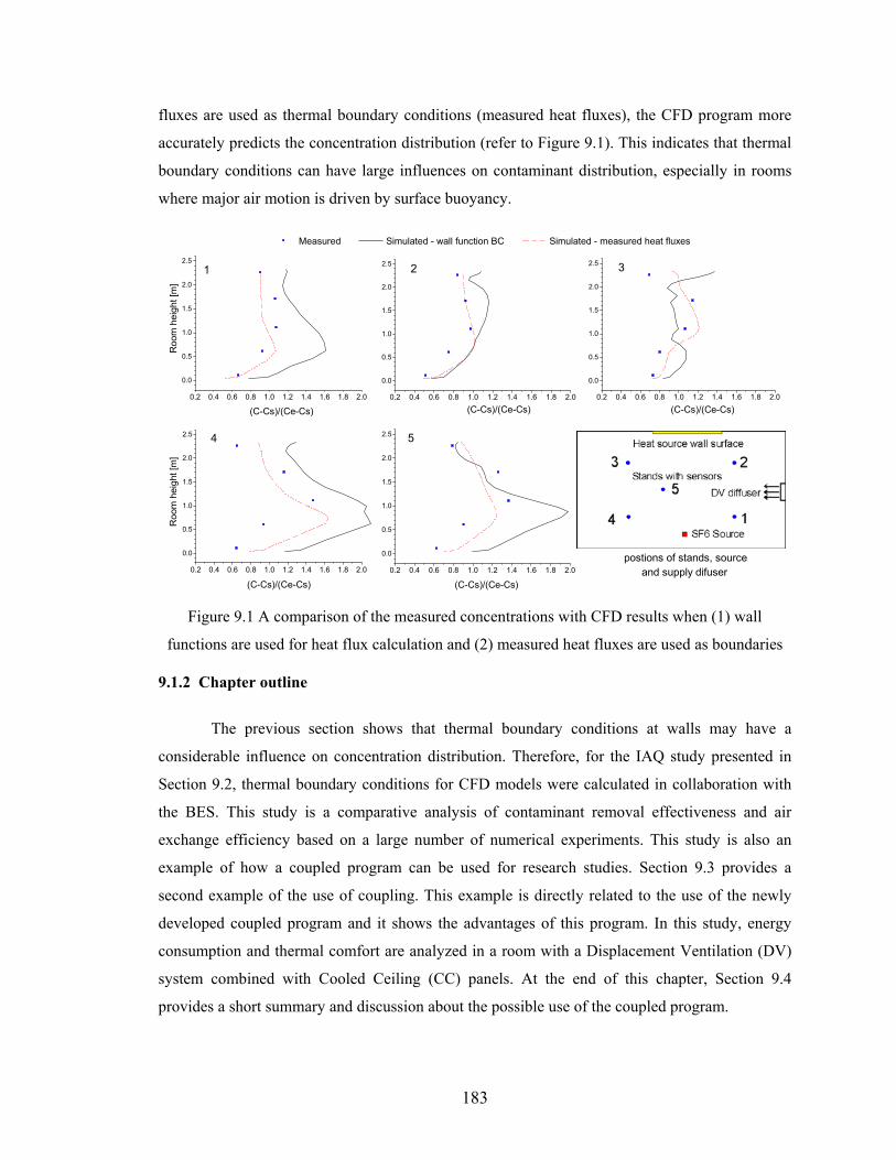
183

fluxes are used as thermal boundary conditions (measured heat fluxes), the CFD program more

accurately predicts the concentration distribution (refer to Figure 9.1). This indicates that thermal

boundary conditions can have large influences on contaminant distribution, especially in rooms

where major air motion is driven by surface buoyancy.

0.2 0.4 0.6 0.8 1.0 1.2 1.4 1.6 1.8 2.0

0.0

0.5

1.0

1.5

2.0

2.51 3

54

Measured Simulated - wall function BC Simulated - measured heat fluxes

Roo

m h

eigh

t [m

]

(C-Cs)/(Ce-Cs)0.2 0.4 0.6 0.8 1.0 1.2 1.4 1.6 1.8 2.0

0.0

0.5

1.0

1.5

2.0

2.5 2

(C-Cs)/(Ce-Cs)0.2 0.4 0.6 0.8 1.0 1.2 1.4 1.6 1.8 2.0

0.0

0.5

1.0

1.5

2.0

2.5

(C-Cs)/(Ce-Cs)

0.2 0.4 0.6 0.8 1.0 1.2 1.4 1.6 1.8 2.0

0.0

0.5

1.0

1.5

2.0

2.5

postions of stands, source and supply difuser

Roo

m h

eigh

t [m

]

(C-Cs)/(Ce-Cs)0.2 0.4 0.6 0.8 1.0 1.2 1.4 1.6 1.8 2.0

0.0

0.5

1.0

1.5

2.0

2.5

(C-Cs)/(Ce-Cs) Figure 9.1 A comparison of the measured concentrations with CFD results when (1) wall

functions are used for heat flux calculation and (2) measured heat fluxes are used as boundaries

9.1.2 Chapter outline

The previous section shows that thermal boundary conditions at walls may have a

considerable influence on concentration distribution. Therefore, for the IAQ study presented in

Section 9.2, thermal boundary conditions for CFD models were calculated in collaboration with

the BES. This study is a comparative analysis of contaminant removal effectiveness and air

exchange efficiency based on a large number of numerical experiments. This study is also an

example of how a coupled program can be used for research studies. Section 9.3 provides a

second example of the use of coupling. This example is directly related to the use of the newly

developed coupled program and it shows the advantages of this program. In this study, energy

consumption and thermal comfort are analyzed in a room with a Displacement Ventilation (DV)

system combined with Cooled Ceiling (CC) panels. At the end of this chapter, Section 9.4

provides a short summary and discussion about the possible use of the coupled program.

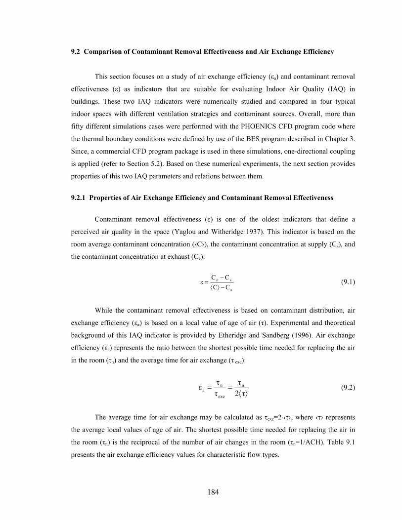
184

9.2 Comparison of Contaminant Removal Effectiveness and Air Exchange Efficiency

This section focuses on a study of air exchange efficiency (εa) and contaminant removal

effectiveness (ε) as indicators that are suitable for evaluating Indoor Air Quality (IAQ) in

buildings. These two IAQ indicators were numerically studied and compared in four typical

indoor spaces with different ventilation strategies and contaminant sources. Overall, more than

fifty different simulations cases were performed with the PHOENICS CFD program code where

the thermal boundary conditions were defined by use of the BES program described in Chapter 3.

Since, a commercial CFD program package is used in these simulations, one-directional coupling

is applied (refer to Section 5.2). Based on these numerical experiments, the next section provides

properties of this two IAQ parameters and relations between them.

9.2.1 Properties of Air Exchange Efficiency and Contaminant Removal Effectiveness

Contaminant removal effectiveness (ε) is one of the oldest indicators that define a

perceived air quality in the space (Yaglou and Witheridge 1937). This indicator is based on the

room average contaminant concentration (‹C›), the contaminant concentration at supply (Cs), and

the contaminant concentration at exhaust (Ce):

s

se

CCCC

ε−⟩⟨−

= (9.1)

While the contaminant removal effectiveness is based on contaminant distribution, air

exchange efficiency (εa) is based on a local value of age of air (τ). Experimental and theoretical

background of this IAQ indicator is provided by Etheridge and Sandberg (1996). Air exchange

efficiency (εa) represents the ratio between the shortest possible time needed for replacing the air

in the room (τn) and the average time for air exchange (τ exe):

⟩⟨==

τ2τ

ττε n

exe

na (9.2)

The average time for air exchange may be calculated as τexe=2·‹τ›, where ‹τ› represents

the average local values of age of air. The shortest possible time needed for replacing the air in

the room (τn) is the reciprocal of the number of air changes in the room (τn=1/ACH). Table 9.1

presents the air exchange efficiency values for characteristic flow types.

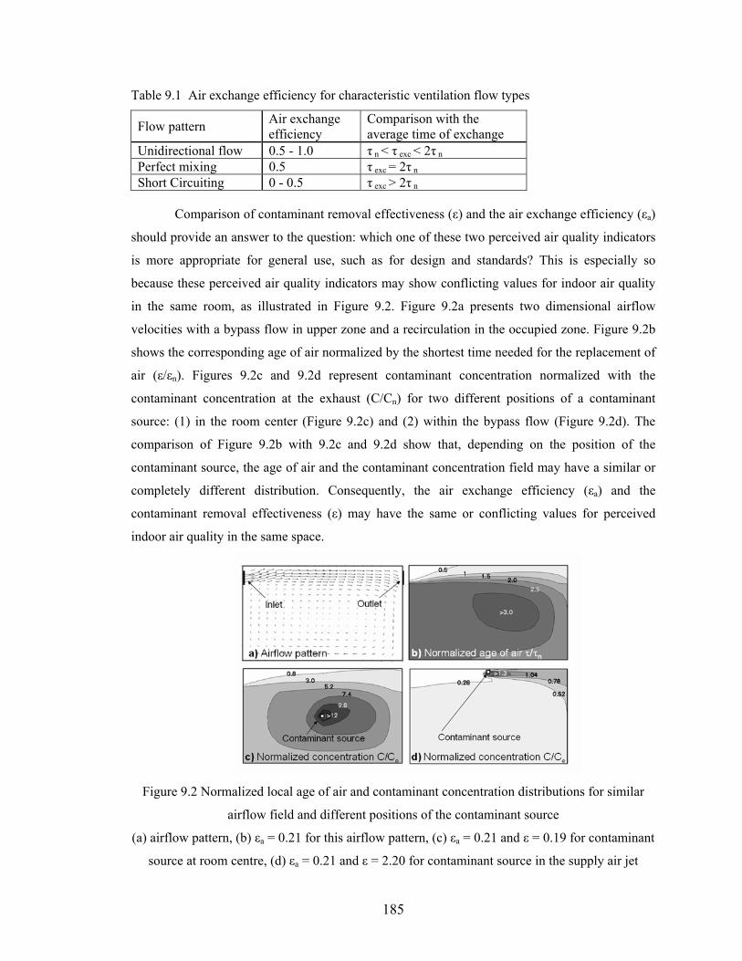
185

Table 9.1 Air exchange efficiency for characteristic ventilation flow types

Flow pattern Air exchange efficiency

Comparison with the average time of exchange

Unidirectional flow 0.5 - 1.0 τ n < τ exc < 2τ n Perfect mixing 0.5 τ exc = 2τ n Short Circuiting 0 - 0.5 τ exc > 2τ n

Comparison of contaminant removal effectiveness (ε) and the air exchange efficiency (εa)

should provide an answer to the question: which one of these two perceived air quality indicators

is more appropriate for general use, such as for design and standards? This is especially so

because these perceived air quality indicators may show conflicting values for indoor air quality

in the same room, as illustrated in Figure 9.2. Figure 9.2a presents two dimensional airflow

velocities with a bypass flow in upper zone and a recirculation in the occupied zone. Figure 9.2b

shows the corresponding age of air normalized by the shortest time needed for the replacement of

air (ε/εn). Figures 9.2c and 9.2d represent contaminant concentration normalized with the

contaminant concentration at the exhaust (C/Cn) for two different positions of a contaminant

source: (1) in the room center (Figure 9.2c) and (2) within the bypass flow (Figure 9.2d). The

comparison of Figure 9.2b with 9.2c and 9.2d show that, depending on the position of the

contaminant source, the age of air and the contaminant concentration field may have a similar or

completely different distribution. Consequently, the air exchange efficiency (εa) and the

contaminant removal effectiveness (ε) may have the same or conflicting values for perceived

indoor air quality in the same space.

Figure 9.2 Normalized local age of air and contaminant concentration distributions for similar

airflow field and different positions of the contaminant source

(a) airflow pattern, (b) εa = 0.21 for this airflow pattern, (c) εa = 0.21 and ε = 0.19 for contaminant

source at room centre, (d) εa = 0.21 and ε = 2.20 for contaminant source in the supply air jet

186

The discrepancies in the concentration and age of air distribution patterns result in

conflicting values of εa and ε with different positions of the contaminant source (refer to Figure

9.2). The differences in values of εa and ε are due to the different “nature” of these two indicators.

The air exchange efficiency is an indicator of air distribution quality because it quantifies how

good the air flow pattern is. This efficiency indicator accounts for the size and intensity of the

recirculation in the room by comparing the room airflow pattern with the airflow pattern of the

ideal piston flow. On the other hand, the contaminant removal effectiveness is the indicator of

contamination level in a room. The effectiveness indicator depends not only on the airflow

pattern, but also on the intensity, area, and positions of contaminant sources relative to this

airflow pattern.

Equations (9.1) and (9.2) also demonstrate the different physical meaning of the contaminant

removal effectiveness and the air exchange efficiency, thus rendering a direct comparison

meaningless. The air exchange efficiency has values from 0 to 1, while the contaminants removal

effectiveness takes values from 0 to infinity. Table 9.2 shows ventilation cases for which ε and εa

values approach their lower and upper limits.

Table 9.2 Limits for air exchange efficiency and contaminants removal effectiveness

Upper limit εa = 1 Ideal piston flow Perfect mixing εa = 0.5 Complete and instantaneous mixing

Air exchange efficiency Lower limit εa → 0 Bypass area and recirculation area are completely separated

Upper limit ε → ∞ Contaminant source at the outlet Flow field does not have influence

Perfect mixing ε = 1 Complete and instantaneous mixing Position of contaminant does not have influence

Contaminant removal

effectiveness Lower limit ε → 0

Contaminant source is in the recirculation area which is completely separated from the bypass area

The contaminant removal effectiveness depends not only on the position of the

contaminant relative to the airflow pattern, but also on the area of the source region. For example,

a contaminant may be released from a point source such as tobacco smoke or from a large area

source such as pollutants from a floor finish. Furthermore, contaminant removal effectiveness

depends on source properties such as contaminant density. Consequently, it is hard to expect a

relationship between ε and εa (Sandberg and Sjoberg 1984, and Skaret 1984) because the number

of combinations of flow patterns and type and positions of the contaminant sources are unlimited.

However, for typical spaces usually found in buildings, there are a limited number of ventilation

strategies with common types of contaminants and their positions. Therefore, the number of

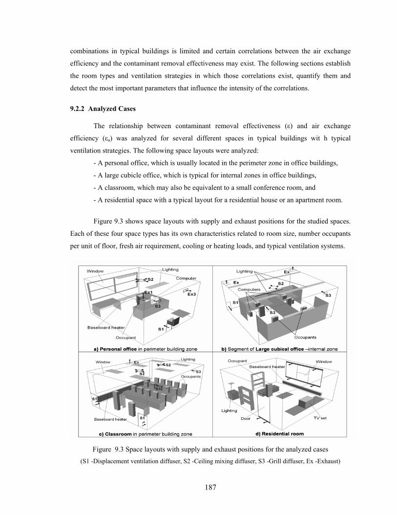
187

combinations in typical buildings is limited and certain correlations between the air exchange

efficiency and the contaminant removal effectiveness may exist. The following sections establish

the room types and ventilation strategies in which those correlations exist, quantify them and

detect the most important parameters that influence the intensity of the correlations.

9.2.2 Analyzed Cases

The relationship between contaminant removal effectiveness (ε) and air exchange

efficiency (εa) was analyzed for several different spaces in typical buildings wit h typical

ventilation strategies. The following space layouts were analyzed:

- A personal office, which is usually located in the perimeter zone in office buildings,

- A large cubicle office, which is typical for internal zones in office buildings,

- A classroom, which may also be equivalent to a small conference room, and

- A residential space with a typical layout for a residential house or an apartment room.

Figure 9.3 shows space layouts with supply and exhaust positions for the studied spaces.

Each of these four space types has its own characteristics related to room size, number occupants

per unit of floor, fresh air requirement, cooling or heating loads, and typical ventilation systems.

Figure 9.3 Space layouts with supply and exhaust positions for the analyzed cases

(S1 -Displacement ventilation diffuser, S2 -Ceiling mixing diffuser, S3 -Grill diffuser, Ex -Exhaust)

188

The number of occupants determines the required amount of fresh air, which together

with heating/cooling loads, has a considerable influence on the selection of a ventilation system.

For example, the personal office has a small occupancy rate and relatively high cooling load per

unit of area, which results in small flow rates of fresh air and large total supply air flow rates for

all-air systems. On the other hand, in cases where heating/cooling loads are treated with a

perimeter heater, fan coil or chilled ceiling, only fresh air is supplied to save fan energy. The

large cubicle office has a large occupancy per unit of floor, but also very large cooling loads.

Therefore, for this type of room and all-air systems, the amount of supply air is usually

determined by cooling loads. In classrooms or small conference rooms, the number of occupants

per unit of floor area is large and the amount of supply air is determined by the required amount

of fresh air per occupant. Consequently, this type of spaces usually does not have recirculation.

Finally, in the case of residential rooms, the occupancy is typically low and ventilation is usually

accomplished by infiltration when the outdoor temperature is low or by an open window where

the outdoor climate and noise conditions are acceptable.

Based on the cooling or heating loads and the amount of supply air, several ventilation

strategies were selected for each of the analyzed spaces. These ventilation strategies determined

the position and type of supplies and exhausts (S1, S2, S3, and Ex in Figure 9.3). The analyzed

ventilation strategies are displacement ventilation, displacement ventilation combined with cooled

ceiling, mixing ventilation with ceiling diffuser, mixing ventilation with grill diffusers,

displacement diffuse combined with baseboard heater, ceiling diffuser combined with baseboard

heater, ceiling diffuser for all air heating, natural ventilation with open window, natural

ventilation with infiltration and heating by baseboard heater, and natural ventilation with

infiltration and air heating supply below window. Table 9.3 contains the important parameters for

all these cases. In some cases, the total convective loads differ from air loads due to the installed

chilled ceiling or baseboard heater or in cases with an all-air heating system due to internal heat

sources. In the Table 9.3, the “Total convective load” indicates the intensity of buoyancy driven

flow in the room, while the “Air load” indicates a fraction of the total convective load removed

by air. A negative value for total convective loads indicates that heating in the room is needed,

while a negative value for air loads shows that the supply air has larger temperature than the

exhaust air. The level of thermal comfort in each analyzed case is approximately the same. The

last column in Table 9.3 shows the difference between the supply air and average room

temperatures.

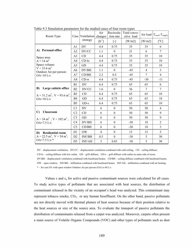
189

Table 9.3 Simulation parameters for the studied cases of four room types

Air changes

Recircula-tion rate

Total conve- ctive load Air load Troom-Tsupply

Room Type

Case

Ventilation

strategy [h-1] [-] [W/m2] [W/m2] [oC]

A1 DV 4.4 0.75 35 35 6 A2 DV/CC 1.1 0 21 6 7 A3 CD 4.4 0.75 35 35 10 A4 CD-lo 4.4 0.75 35 35 10 A5 GD 4.4 0.75 35 35 10 A6 DV/BH 1.1 0 -45 4 3 A7 CD/BH 2.2 0.5 -45 7 4

A) Personal office Space area: A = 14 m2 Space volume: V = 33.6 m3 Outdoor Air per person: OA=10 L/s

A8 CD-w 4.4 0.75 -45 -30 -11 B1 DV 6.4 0.75 65 65 6 B2 DV/CC 1.6 0 36 7 7 B3 CD 6.4 0.75 65 65 10 B4 GD 6.4 0.75 65 65 10

B) Large cubicle office A = 31.2 m2, V = 93.6 m3, OA=10 L/s

B5 GD-s 6.4 0.75 65 65 10 C1 DV 6 0 50 50 4 C2 CD 6 0 50 50 9 C3 GD 6 0 50 50 9 C4 DV/BH 6 0 -30 18 2

C) Classroom A = 34 m2 , V = 102 m3 , OA=7.5 L/s

C5 CD/BH 6 0 -30 18 3 D1 OW 4 0 15 15 5 D2 INF/BH 0.5 0 -38 5 30

D) Residential room A = 22.5 m2, V = 54 m3, OA=7.5 L/s * D3 INF/AH 3 0.83 -38 5 30

DV – displacement ventilation, DV/CC – displacement ventilation combined with cold ceiling, CD – ceiling diffuser,

CD-lo – ceiling diffuser with low outlet, GD – grill diffuser, GD-s – grill diffuser with outlet on same side of room,

DV/BH – displacement ventilation combined with baseboard heater, CD/BH – ceiling diffuser combined with baseboard heater,

OW – open window, INF/BH – infiltration combined with baseboard heater, INF/AH – infiltration combined with air heating,

* – for case D1 with open window Outdoor Air per person (OA) is 60 L/s

Values ε and εa for active and passive contaminant sources were calculated for all cases.

To study active types of pollutants that are associated with heat sources, the distribution of

contaminant released in the vicinity of an occupant’s head was analyzed. This contaminant may

represent tobacco smoke, CO2, or any human bioeffluent. On the other hand, passive pollutants

are not directly moved with thermal plumes of heat sources because of their position relative to

the heat sources or size of the source area. To evaluate the transport of passive pollutants the

distribution of contaminants released from a carpet was analyzed. Moreover, carpets often present

a main source of Volatile Organic Compounds (VOC) and other types of pollutants such as dust

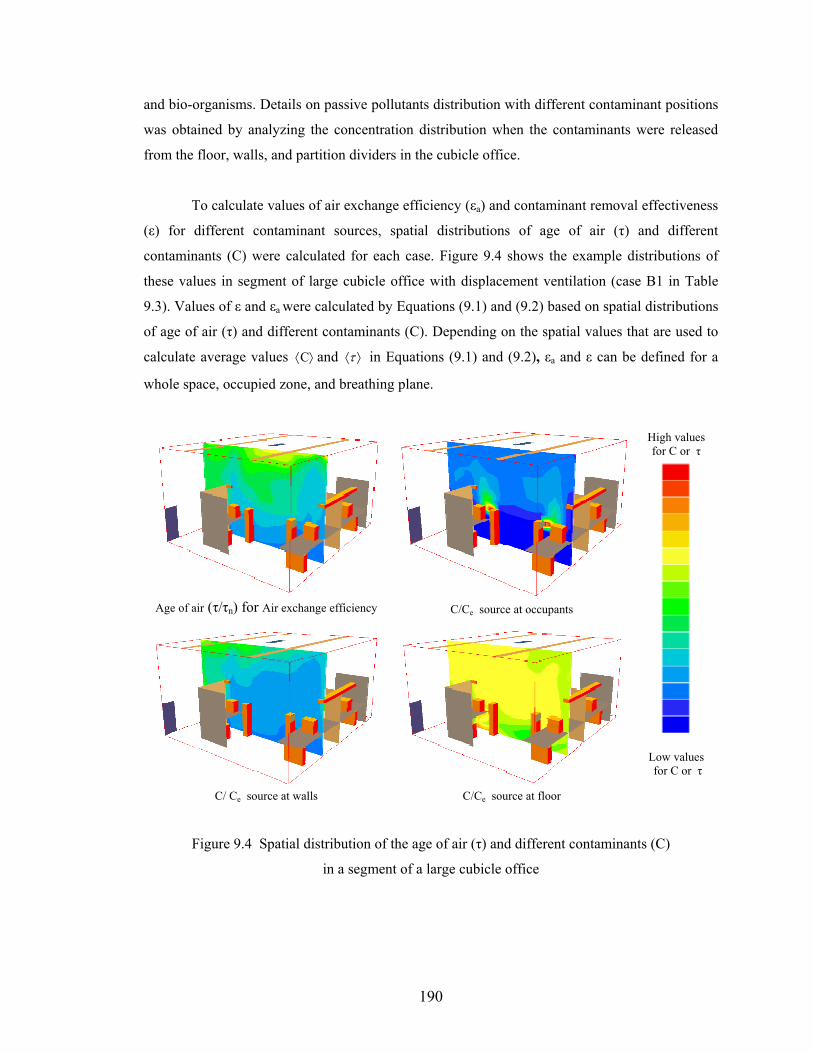
190

and bio-organisms. Details on passive pollutants distribution with different contaminant positions

was obtained by analyzing the concentration distribution when the contaminants were released

from the floor, walls, and partition dividers in the cubicle office.

To calculate values of air exchange efficiency (εa) and contaminant removal effectiveness

(ε) for different contaminant sources, spatial distributions of age of air (τ) and different

contaminants (C) were calculated for each case. Figure 9.4 shows the example distributions of

these values in segment of large cubicle office with displacement ventilation (case B1 in Table

9.3). Values of ε and εa were calculated by Equations (9.1) and (9.2) based on spatial distributions

of age of air (τ) and different contaminants (C). Depending on the spatial values that are used to

calculate average values ⟩⟨C and ⟩⟨τ in Equations (9.1) and (9.2), εa and ε can be defined for a

whole space, occupied zone, and breathing plane.

Age of air (τ/τn) for Air exchange efficiency C/Ce source at occupants

C/ Ce source at walls C/Ce source at floor

High values for C or τ

Low values for C or τ

Figure 9.4 Spatial distribution of the age of air (τ) and different contaminants (C)

in a segment of a large cubicle office

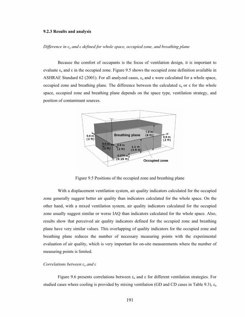
191

9.2.3 Results and analysis

Difference in εa and ε defined for whole space, occupied zone, and breathing plane

Because the comfort of occupants is the focus of ventilation design, it is important to

evaluate εa and ε in the occupied zone. Figure 9.5 shows the occupied zone definition available in

ASHRAE Standard 62 (2001). For all analyzed cases, εa and ε were calculated for a whole space,

occupied zone and breathing plane. The difference between the calculated εa or ε for the whole

space, occupied zone and breathing plane depends on the space type, ventilation strategy, and

position of contaminant sources.

Figure 9.5 Positions of the occupied zone and breathing plane

With a displacement ventilation system, air quality indicators calculated for the occupied

zone generally suggest better air quality than indicators calculated for the whole space. On the

other hand, with a mixed ventilation system, air quality indicators calculated for the occupied

zone usually suggest similar or worse IAQ than indicators calculated for the whole space. Also,

results show that perceived air quality indicators defined for the occupied zone and breathing

plane have very similar values. This overlapping of quality indicators for the occupied zone and

breathing plane reduces the number of necessary measuring points with the experimental

evaluation of air quality, which is very important for on-site measurements where the number of

measuring points is limited.

Correlations between εa and ε

Figure 9.6 presents correlations between εa and ε for different ventilation strategies. For

studied cases where cooling is provided by mixing ventilation (GD and CD cases in Table 9.3), εa

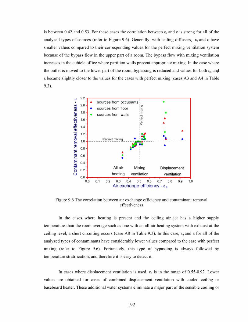
192

is between 0.42 and 0.53. For these cases the correlation between εa and ε is strong for all of the

analyzed types of sources (refer to Figure 9.6). Generally, with ceiling diffusers, εa and ε have

smaller values compared to their corresponding values for the perfect mixing ventilation system

because of the bypass flow in the upper part of a room. The bypass flow with mixing ventilation

increases in the cubicle office where partition walls prevent appropriate mixing. In the case where

the outlet is moved to the lower part of the room, bypassing is reduced and values for both εa and

ε became slightly closer to the values for the cases with perfect mixing (cases A3 and A4 in Table

9.3).

0.0 0.1 0.2 0.3 0.4 0.5 0.6 0.7 0.8 0.9 1.00.0

0.2

0.4

0.6

0.8

1.0

1.2

1.4

1.6

1.8

2.0

2.2

a

Per

fect

mix

ing

Perfect mixing

All airheating

Displacement ventilation

Mixingventilation

sources from occupants sources from floor sources from walls

Con

tam

inan

t rem

oval

effe

ctiv

enes

s - ε

Air exchange efficiency - ε

Figure 9.6 The correlation between air exchange efficiency and contaminant removal effectiveness

In the cases where heating is present and the ceiling air jet has a higher supply

temperature than the room average such as one with an all-air heating system with exhaust at the

ceiling level, a short circuiting occurs (case A8 in Table 9.3). In this case, εa and ε for all of the

analyzed types of contaminants have considerably lower values compared to the case with perfect

mixing (refer to Figure 9.6). Fortunately, this type of bypassing is always followed by

temperature stratification, and therefore it is easy to detect it.

In cases where displacement ventilation is used, εa is in the range of 0.55-0.92. Lower

values are obtained for cases of combined displacement ventilation with cooled ceiling or

baseboard heater. These additional water systems eliminate a major part of the sensible cooling or

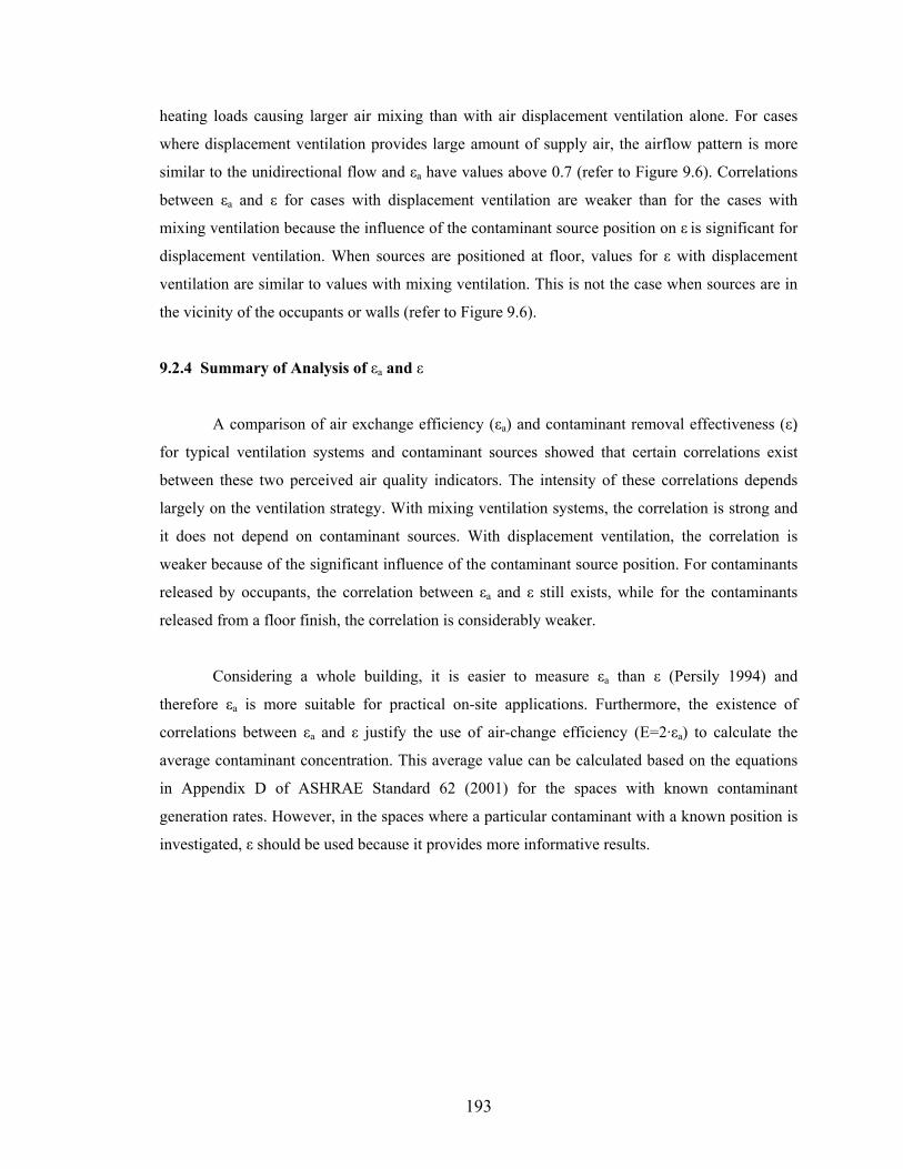
193

heating loads causing larger air mixing than with air displacement ventilation alone. For cases

where displacement ventilation provides large amount of supply air, the airflow pattern is more

similar to the unidirectional flow and εa have values above 0.7 (refer to Figure 9.6). Correlations

between εa and ε for cases with displacement ventilation are weaker than for the cases with

mixing ventilation because the influence of the contaminant source position on ε is significant for

displacement ventilation. When sources are positioned at floor, values for ε with displacement

ventilation are similar to values with mixing ventilation. This is not the case when sources are in

the vicinity of the occupants or walls (refer to Figure 9.6).

9.2.4 Summary of Analysis of εa and ε

A comparison of air exchange efficiency (εa) and contaminant removal effectiveness (ε)

for typical ventilation systems and contaminant sources showed that certain correlations exist

between these two perceived air quality indicators. The intensity of these correlations depends

largely on the ventilation strategy. With mixing ventilation systems, the correlation is strong and

it does not depend on contaminant sources. With displacement ventilation, the correlation is

weaker because of the significant influence of the contaminant source position. For contaminants

released by occupants, the correlation between εa and ε still exists, while for the contaminants

released from a floor finish, the correlation is considerably weaker.

Considering a whole building, it is easier to measure εa than ε (Persily 1994) and

therefore εa is more suitable for practical on-site applications. Furthermore, the existence of

correlations between εa and ε justify the use of air-change efficiency (E=2·εa) to calculate the

average contaminant concentration. This average value can be calculated based on the equations

in Appendix D of ASHRAE Standard 62 (2001) for the spaces with known contaminant

generation rates. However, in the spaces where a particular contaminant with a known position is

investigated, ε should be used because it provides more informative results.

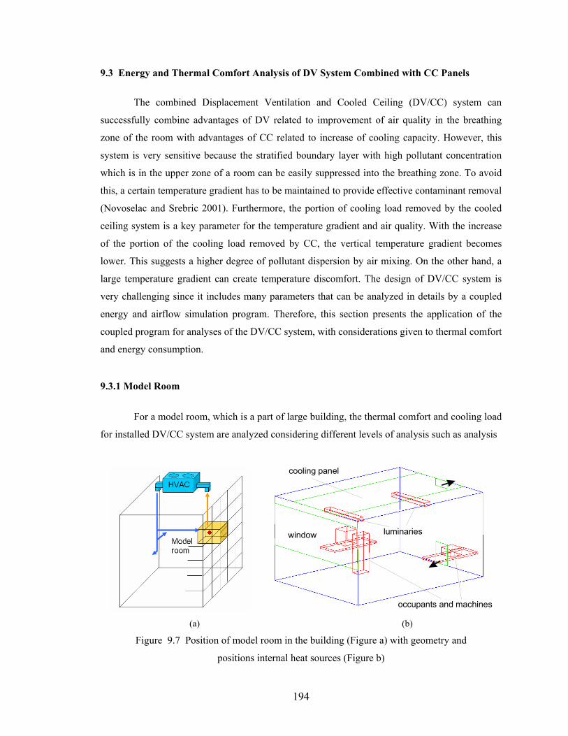
194

9.3 Energy and Thermal Comfort Analysis of DV System Combined with CC Panels

The combined Displacement Ventilation and Cooled Ceiling (DV/CC) system can

successfully combine advantages of DV related to improvement of air quality in the breathing

zone of the room with advantages of CC related to increase of cooling capacity. However, this

system is very sensitive because the stratified boundary layer with high pollutant concentration

which is in the upper zone of a room can be easily suppressed into the breathing zone. To avoid

this, a certain temperature gradient has to be maintained to provide effective contaminant removal

(Novoselac and Srebric 2001). Furthermore, the portion of cooling load removed by the cooled

ceiling system is a key parameter for the temperature gradient and air quality. With the increase

of the portion of the cooling load removed by CC, the vertical temperature gradient becomes

lower. This suggests a higher degree of pollutant dispersion by air mixing. On the other hand, a

large temperature gradient can create temperature discomfort. The design of DV/CC system is

very challenging since it includes many parameters that can be analyzed in details by a coupled

energy and airflow simulation program. Therefore, this section presents the application of the

coupled program for analyses of the DV/CC system, with considerations given to thermal comfort

and energy consumption.

9.3.1 Model Room

For a model room, which is a part of large building, the thermal comfort and cooling load

for installed DV/CC system are analyzed considering different levels of analysis such as analysis

occupants and machines

window

cooling panel

luminaries

(a) (b)

Figure 9.7 Position of model room in the building (Figure a) with geometry and

positions internal heat sources (Figure b)

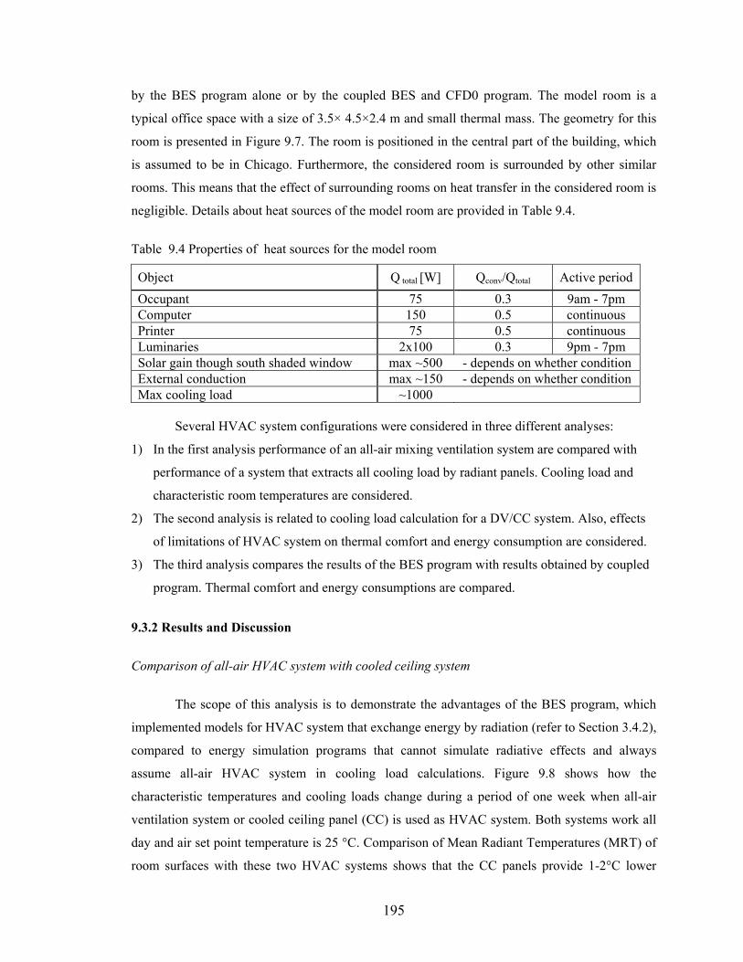
195

by the BES program alone or by the coupled BES and CFD0 program. The model room is a

typical office space with a size of 3.5× 4.5×2.4 m and small thermal mass. The geometry for this

room is presented in Figure 9.7. The room is positioned in the central part of the building, which

is assumed to be in Chicago. Furthermore, the considered room is surrounded by other similar

rooms. This means that the effect of surrounding rooms on heat transfer in the considered room is

negligible. Details about heat sources of the model room are provided in Table 9.4.

Table 9.4 Properties of heat sources for the model room

Object Q total [W] Qconv/Qtotal Active period Occupant 75 0.3 9am - 7pm Computer 150 0.5 continuous Printer 75 0.5 continuous Luminaries 2x100 0.3 9pm - 7pm Solar gain though south shaded window max ~500 - depends on whether condition External conduction max ~150 - depends on whether condition Max cooling load ~1000

Several HVAC system configurations were considered in three different analyses:

1) In the first analysis performance of an all-air mixing ventilation system are compared with

performance of a system that extracts all cooling load by radiant panels. Cooling load and

characteristic room temperatures are considered.

2) The second analysis is related to cooling load calculation for a DV/CC system. Also, effects

of limitations of HVAC system on thermal comfort and energy consumption are considered.

3) The third analysis compares the results of the BES program with results obtained by coupled

program. Thermal comfort and energy consumptions are compared.

9.3.2 Results and Discussion Comparison of all-air HVAC system with cooled ceiling system

The scope of this analysis is to demonstrate the advantages of the BES program, which

implemented models for HVAC system that exchange energy by radiation (refer to Section 3.4.2),

compared to energy simulation programs that cannot simulate radiative effects and always

assume all-air HVAC system in cooling load calculations. Figure 9.8 shows how the

characteristic temperatures and cooling loads change during a period of one week when all-air

ventilation system or cooled ceiling panel (CC) is used as HVAC system. Both systems work all

day and air set point temperature is 25 °C. Comparison of Mean Radiant Temperatures (MRT) of

room surfaces with these two HVAC systems shows that the CC panels provide 1-2°C lower

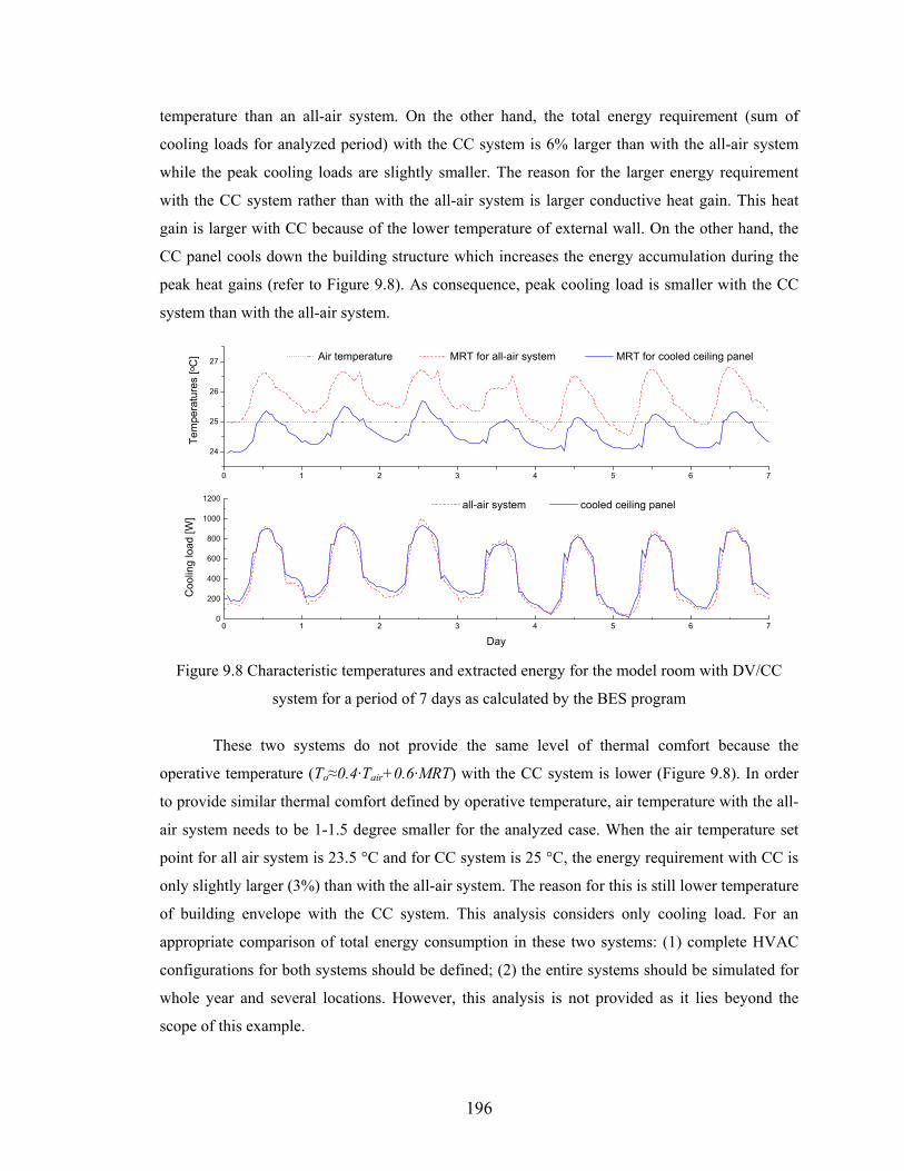
196

temperature than an all-air system. On the other hand, the total energy requirement (sum of

cooling loads for analyzed period) with the CC system is 6% larger than with the all-air system

while the peak cooling loads are slightly smaller. The reason for the larger energy requirement

with the CC system rather than with the all-air system is larger conductive heat gain. This heat

gain is larger with CC because of the lower temperature of external wall. On the other hand, the

CC panel cools down the building structure which increases the energy accumulation during the

peak heat gains (refer to Figure 9.8). As consequence, peak cooling load is smaller with the CC

system than with the all-air system.

0 1 2 3 4 5 6 70

200

400

600

800

1000

1200 all-air system cooled ceiling panel

Coo

ling

load

[W]

Day

0 1 2 3 4 5 6 7

24

25

26

27

Tem

pera

ture

s [o

C] Air temperature MRT for all-air system MRT for cooled ceiling panel

Figure 9.8 Characteristic temperatures and extracted energy for the model room with DV/CC

system for a period of 7 days as calculated by the BES program

These two systems do not provide the same level of thermal comfort because the

operative temperature (To≈0.4·Tair+0.6·MRT) with the CC system is lower (Figure 9.8). In order

to provide similar thermal comfort defined by operative temperature, air temperature with the all-

air system needs to be 1-1.5 degree smaller for the analyzed case. When the air temperature set

point for all air system is 23.5 °C and for CC system is 25 °C, the energy requirement with CC is

only slightly larger (3%) than with the all-air system. The reason for this is still lower temperature

of building envelope with the CC system. This analysis considers only cooling load. For an

appropriate comparison of total energy consumption in these two systems: (1) complete HVAC

configurations for both systems should be defined; (2) the entire systems should be simulated for

whole year and several locations. However, this analysis is not provided as it lies beyond the

scope of this example.

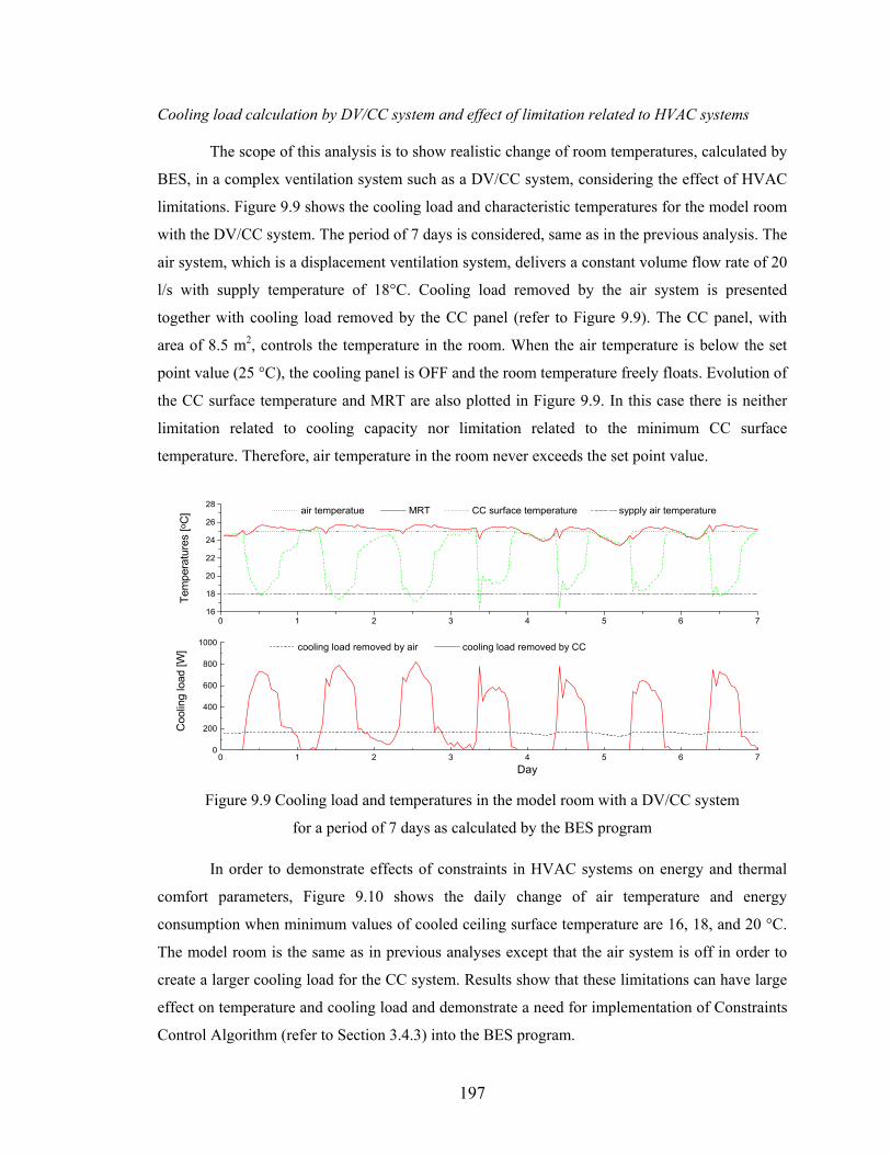
197

Cooling load calculation by DV/CC system and effect of limitation related to HVAC systems The scope of this analysis is to show realistic change of room temperatures, calculated by

BES, in a complex ventilation system such as a DV/CC system, considering the effect of HVAC

limitations. Figure 9.9 shows the cooling load and characteristic temperatures for the model room

with the DV/CC system. The period of 7 days is considered, same as in the previous analysis. The

air system, which is a displacement ventilation system, delivers a constant volume flow rate of 20

l/s with supply temperature of 18°C. Cooling load removed by the air system is presented

together with cooling load removed by the CC panel (refer to Figure 9.9). The CC panel, with

area of 8.5 m2, controls the temperature in the room. When the air temperature is below the set

point value (25 °C), the cooling panel is OFF and the room temperature freely floats. Evolution of

the CC surface temperature and MRT are also plotted in Figure 9.9. In this case there is neither

limitation related to cooling capacity nor limitation related to the minimum CC surface

temperature. Therefore, air temperature in the room never exceeds the set point value.

0 1 2 3 4 5 6 70

200

400

600

800

1000 cooling load removed by air cooling load removed by CC

Coo

ling

load

[W]

Day

0 1 2 3 4 5 6 716

18

20

22

24

26

28

Tem

pera

ture

s [o

C] air temperatue MRT CC surface temperature sypply air temperature

Figure 9.9 Cooling load and temperatures in the model room with a DV/CC system

for a period of 7 days as calculated by the BES program In order to demonstrate effects of constraints in HVAC systems on energy and thermal

comfort parameters, Figure 9.10 shows the daily change of air temperature and energy

consumption when minimum values of cooled ceiling surface temperature are 16, 18, and 20 °C.

The model room is the same as in previous analyses except that the air system is off in order to

create a larger cooling load for the CC system. Results show that these limitations can have large

effect on temperature and cooling load and demonstrate a need for implementation of Constraints

Control Algorithm (refer to Section 3.4.3) into the BES program.

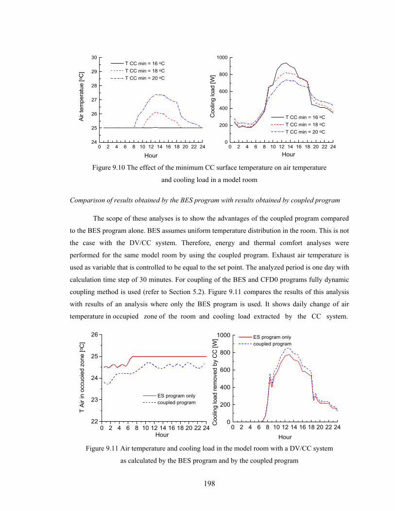
198

0 2 4 6 8 10 12 14 16 18 20 22 2424

25

26

27

28

29

30

Hour

T CC min = 16 oC T CC min = 18 oC T CC min = 20 oC

Air

tem

pera

tue

[oC

]

Hour0 2 4 6 8 10 12 14 16 18 20 22 24

0

200

400

600

800

1000

Coo

ling

load

[W]

T CC min = 16 oC T CC min = 18 oC T CC min = 20 oC

Figure 9.10 The effect of the minimum CC surface temperature on air temperature

and cooling load in a model room

Comparison of results obtained by the BES program with results obtained by coupled program The scope of these analyses is to show the advantages of the coupled program compared

to the BES program alone. BES assumes uniform temperature distribution in the room. This is not

the case with the DV/CC system. Therefore, energy and thermal comfort analyses were

performed for the same model room by using the coupled program. Exhaust air temperature is

used as variable that is controlled to be equal to the set point. The analyzed period is one day with

calculation time step of 30 minutes. For coupling of the BES and CFD0 programs fully dynamic

coupling method is used (refer to Section 5.2). Figure 9.11 compares the results of this analysis

with results of an analysis where only the BES program is used. It shows daily change of air

temperature in occupied zone of the room and cooling load extracted by the CC system.

0 2 4 6 8 10 12 14 16 18 20 22 240

200

400

600

800

1000

T A

ir in

occ

uoie

d zo

ne [o

C]

Hour

ES program only coupled program

Coo

ling

load

rem

oved

by

CC

[W]

Hour0 2 4 6 8 10 12 14 16 18 20 22 24

22

23

24

25

26

ES program only coupled program

Figure 9.11 Air temperature and cooling load in the model room with a DV/CC system

as calculated by the BES program and by the coupled program

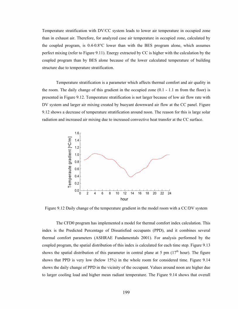
199

Temperature stratification with DV/CC system leads to lower air temperature in occupied zone

than in exhaust air. Therefore, for analyzed case air temperature in occupied zone, calculated by

the coupled program, is 0.4-0.8°C lower than with the BES program alone, which assumes

perfect mixing (refer to Figure 9.11). Energy extracted by CC is higher with the calculation by the

coupled program than by BES alone because of the lower calculated temperature of building

structure due to temperature stratification.

Temperature stratification is a parameter which affects thermal comfort and air quality in

the room. The daily change of this gradient in the occupied zone (0.1 - 1.1 m from the floor) is

presented in Figure 9.12. Temperature stratification is not larger because of low air flow rate with

DV system and larger air mixing created by buoyant downward air flow at the CC panel. Figure

9.12 shows a decrease of temperature stratification around noon. The reason for this is large solar

radiation and increased air mixing due to increased convective heat transfer at the CC surface.

0 2 4 6 8 10 12 14 16 18 20 22 240.0

0.2

0.4

0.6

0.8

1.0

1.2

1.4

1.6

Tem

pera

ute

grad

ient

[oC

/m]

hour Figure 9.12 Daily change of the temperature gradient in the model room with a CC/DV system

The CFD0 program has implemented a model for thermal comfort index calculation. This

index is the Predicted Percentage of Dissatisfied occupants (PPD), and it combines several

thermal comfort parameters (ASHRAE Fundamentals 2001). For analysis performed by the

coupled program, the spatial distribution of this index is calculated for each time step. Figure 9.13

shows the spatial distribution of this parameter in central plane at 5 pm (17th hour). The figure

shows that PPD is very low (below 15%) in the whole room for considered time. Figure 9.14

shows the daily change of PPD in the vicinity of the occupant. Values around noon are higher due

to larger cooling load and higher mean radiant temperature. The Figure 9.14 shows that overall

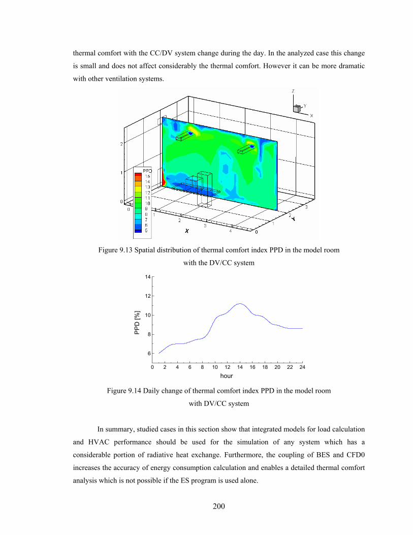
200

thermal comfort with the CC/DV system change during the day. In the analyzed case this change

is small and does not affect considerably the thermal comfort. However it can be more dramatic

with other ventilation systems.

Figure 9.13 Spatial distribution of thermal comfort index PPD in the model room

with the DV/CC system

0 2 4 6 8 10 12 14 16 18 20 22 24

6

8

10

12

14

PP

D [%

]

hour Figure 9.14 Daily change of thermal comfort index PPD in the model room

with DV/CC system

In summary, studied cases in this section show that integrated models for load calculation

and HVAC performance should be used for the simulation of any system which has a

considerable portion of radiative heat exchange. Furthermore, the coupling of BES and CFD0

increases the accuracy of energy consumption calculation and enables a detailed thermal comfort

analysis which is not possible if the ES program is used alone.

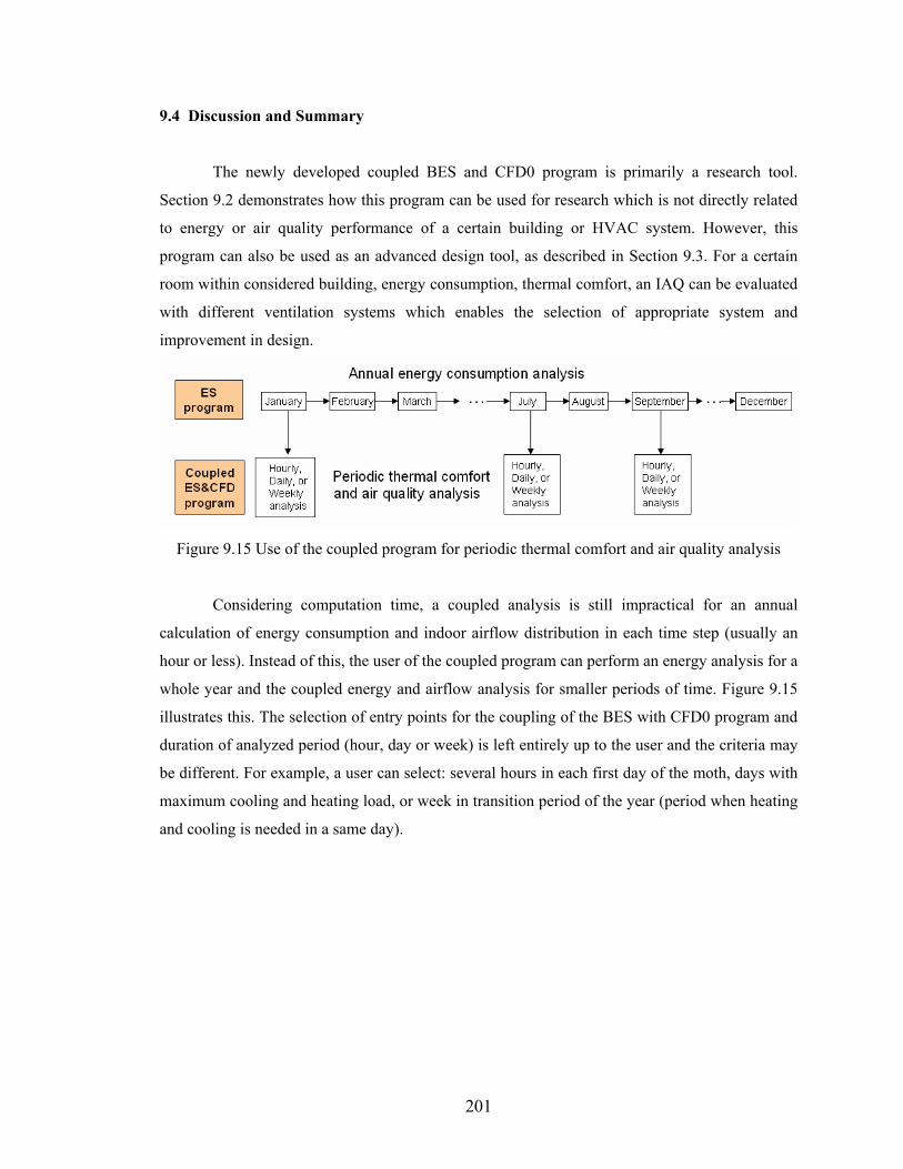
201

9.4 Discussion and Summary

The newly developed coupled BES and CFD0 program is primarily a research tool.

Section 9.2 demonstrates how this program can be used for research which is not directly related

to energy or air quality performance of a certain building or HVAC system. However, this

program can also be used as an advanced design tool, as described in Section 9.3. For a certain

room within considered building, energy consumption, thermal comfort, an IAQ can be evaluated

with different ventilation systems which enables the selection of appropriate system and

improvement in design.

Figure 9.15 Use of the coupled program for periodic thermal comfort and air quality analysis

Considering computation time, a coupled analysis is still impractical for an annual

calculation of energy consumption and indoor airflow distribution in each time step (usually an

hour or less). Instead of this, the user of the coupled program can perform an energy analysis for a

whole year and the coupled energy and airflow analysis for smaller periods of time. Figure 9.15

illustrates this. The selection of entry points for the coupling of the BES with CFD0 program and

duration of analyzed period (hour, day or week) is left entirely up to the user and the criteria may

be different. For example, a user can select: several hours in each first day of the moth, days with

maximum cooling and heating load, or week in transition period of the year (period when heating

and cooling is needed in a same day).

202

CHAPTER 10

CONCLUSIONS AND RECOMMENDATIONS FOR FUTURE RESEARCH

10.1 Conclusions

This section summarizes the main results and conclusions from the research presented in

this thesis. The thesis objective was to enhance the accuracy of indoor air flow and thermal

modeling within the context of a whole-building simulation. The accomplishments of this

research are the following:

(1) new models for air flow and energy simulation in buildings were developed and

existing models were improved,

(2) large amount of experimental data were collected and used for the validation of new

and existing models, and

(3) new software for combined air and energy flow analyses in buildings was developed

and validated.

For the coupling of Energy Simulation (ES) and Computational Fluid Dynamics (CFD)

programs, a new building energy simulation program (BES) was developed. This program

encompasses existing and newly developed models for heat transfer in building components.

With these models, the BES program accurately calculates internal surface temperatures that are

necessary for coupling with the CFD program. Also, a new method for simultaneous load

calculation and HVAC system simulation was developed and implemented in the BES program.

The method enables a modular organization of HVAC system models because HVAC equations

are not integrated into the zone matrix for heat transfer through building envelope. For coupling

of HVAC modules and the zone matrix, a new Constraint Control Algorithm (CCA) was

developed. This algorithm introduces the effect of the HVAC system on building elements by

correcting all temperatures in the calculation domain of the BES program. As result, CCA enables

a better prediction of thermal comfort and HVAC system performance, especially in buildings

where fabric thermal storage has a large influence on energy flow. This includes heating/cooling

slabs and systems with radiant panels. The BES program was extensively validated by several

validation procedures that include energy balance tests and BESTEST procedures. Good

validation results showed that the BES program can be successfully coupled with the airflow

program.

203

An existing CFD program (CFD0 Srebric 2000) was modified for coupling purposes and

further developed by adding improved models for thermal boundary conditions calculations.

Experiment-based correlations were implemented into CFD0 through the Modified Adaptive

Convection Algorithm (MACA). MACA is a modification of the Adaptive Convection Algorithm

- ACA (Beausoleil 2000). ACA was extended by addition of new convection correlations and

further developed for use as a part of CFD0. Experimental validation of MACA showed that this

algorithm and experiment-based correlations provide considerably better accuracy than log-law

wall functions for surface heat flux calculation and air temperature distribution. Thermal

boundary conditions calculated by MACA are still grid-dependent and a variation of 10% in heat

flux may occur. This result is encouraging because 10% variation is much smaller that the

variation of heat fluxes resulting from log-law wall functions grid dependency.

In the analyses related to coupling procedures for ES and CFD programs, issues such as

data transfer methods, difference of the numerical solutions between various coupling methods,

numerical stability, and computation time were considered. Three two-directional coupling

methods with different techniques and dynamics of information exchange between the energy and

airflow programs were analyzed. When appropriate numerical criteria were satisfied, the

difference between numerical solutions calculated by all considered method was insignificant.

The quasi-dynamic coupling is the simplest method, which does not have any problems related to

numerical stability, but it requires small time steps to provide the same numerical solution as the

other methods. The fully dynamic coupling provides numerical solutions that satisfy the energy

balance at surfaces in the ES and CFD domains regardless of time step, but it can be

computationally expensive since it needs many consecutive runs of the CFD program for a single

time step. The integrated coupling method is the most efficient, considering computation time.

However, this method uses CFD results that are not fully converged for data exchange between

the two programs and this can create numerical instability. Generally, quasi-dynamic coupling

should be used for analyses which consider small time periods. Fully dynamic coupling is

suitable for occasional coupled analysis that include coupling for only a few time steps, while for

other time steps just an energy analysis is considered. Integrated coupling can be used in both

types of analyses; however it requires careful selection of calculation step when data in-between

programs are exchanged in order to prevent divergence.

In the course of this thesis, several new convection correlations were developed. These

are convection correlations for rooms with relatively new ventilation systems such as

204

displacement ventilation or mixing ventilation with high aspiration diffusers combined with

radiant cooling panels. These correlations were developed using state-of-the-art experimental

facilities, which enabled measurements in environments such as a representative room in the

building. The measurements of convection coefficients in rooms with analyzed ventilation

systems show that for certain surfaces the existing correlation can be used while for others, the

newly developed correlation should be used. The newly developed convection correlations were

implemented into MACA to improve the accuracy of thermal boundary condition calculations in

CFD analyses for rooms with these relatively new ventilation systems.

Another set of experimental measurements was conducted to validate MACA, together

with eight additional measurements that include experiments with a tracer gas. Experiments were

conducted in a chamber with displacement ventilation, high aspiration diffuser, and heating and

cooling panes. These experimental set-ups emphasized air stratification, air motion due to surface

convection, or mixing by jet with large entrainment of room air. The measured data were

processed and prepared for future use in validation of CFD applications in building analyses.

In this thesis, the coupled program was developed as a tool for accurate energy and

thermal comfort analyses. This is a user-friendly software, which has a newly developed

Graphical User Interface (GUI) and 3D visualization tool for presenting CFD results. The

developed GUI is specialized to provide input data for both BES and CFD0 when they are used

for buildings simulations. Combined with the new 3D visualization tool, GUI enables easy

application of the coupled program for different energy consumption, air quality, and thermal

quality analyses.

Finally, the coupled program was applied to two studies, which demonstrate the

capabilities of this program for use in research and advanced design. The first example is a

comparative analysis of contaminant removal effectiveness and air exchange efficiency based on

a large number of numerical experiments. Based on this analysis, designers can select an

appropriate air quality indicator for their application. The second example shows the advantages

of the couple program for analysis of energy consumption and air quality in a room with

displacement ventilation and cooled ceiling panel. This is the system which includes many

parameters that can be analyzed by the coupled energy and airflow simulation program. The

results of this example show that, by using the coupled program, the accuracy of energy

calculation is increased and the quality of thermal comfort and indoor air quality analysis are

considerably improved.

205

10.2 Recommendations for Future work

This research was focused on developing new and advanced models and tools to simulate

an entire building, accompanied with extensive validation. However, there is much space for

further improvement and validations in this relatively new research area. A few areas identified

for further research are given in the following paragraphs. Further development of MACA

The performance of MACA in CFD is highly dependent on the implemented convection

correlations. Since new ventilation systems are regularly developed, additional convection

correlations for specific air flow are always useful. Also, improvements made to models for

convection correlation selection, based on velocity distribution in near-wall regions, could

improve the applicability of MACA in wide range of airflow regimes in a room.

Improvements in coupling methods

The analysis of the integrated coupling method shows that numerical stability of the

solution procedure depends on the frequency (time steps) of information exchange between the

ES and CFD programs. Additional analyses related to the selection of optimal iteration step for

information exchange could enable faster convergence without problems with numerical

instability. Also, there is a need for algorithm which combines different coupling methods to

obtain optimal compromise between accuracy and computation time.

Further validation and development of the BES program

The current version of the BES program can be used in analyses of single rooms with or

without plenum space. This version of the program can be further developed by advancing and

adding procedures that enable multizone energy simulation. With this improvement the coupled

program would be capable for the analyses that require whole-building simulation.

Implementation and validation of concentration models in CFD0

The current version of CFD0 does not include models for concentration calculation. With

these models, the coupled program would be fully equipped for indoor air quality studies. Using

concentration models, the coupled program would be able to calculate contaminant removal

effectiveness and air exchange efficiency in a whole room, occupied zone, or breathing plane and

provide these data as output. To validate the concentration calculation with the zero equation

turbulence model, the measured data collected as part of this thesis can be used.

206

REFERENCES

Alamdari F. and Hammond G.P. 1983. "Improved Data Correlations for Buoyancy-Driven Convection in Rooms", Building Services Engineering Research and Technology, 4 (3): 106-112. ASHRAE, 1985. “1985 ASHRAE Handbook Fundamentals,” ASHRAE, Atlanta. Ch 28. ASHRAE, 2001. “2001 ASHRAE Handbook Fundamentals,” ASHRAE, Atlanta. ASHRAE. 2001. ASHRAE Standard 62–2001. Ventilation for acceptable indoor air quality. Atlanta: American Society of Heating, Refrigerating and Air-Conditioning Engineers, Inc. Awbi H.B. 1998. "Calculation of Convective Heat Transfer Coefficients of Room Surfaces for Natural Convection", Energy and Buildings, 28: 219-227. Awbi H.B. 1998. “Calculation of convective heat transfer coefficients of room surfaces for natural convection,” Energy and Buildings, 28: 219-227. Awbi H.B. and Hatton A.. 1999. "Natural Convection from Heated Room Surfaces", Energy and Buildings, 30: 233-244. Beausoleil-Morrison I. 2000. “The adaptive coupling of heat and air flow modeling within dynamic whole-building simulation”, PhD Thesis, University of Strathclyde, Glasgow, UK. Beausoleil-Morrison I. and Clarke J. 2003. “An Adaptive Conflation Between CFD and Thermal Simulation for Modeling Indoor Airflow and Convective Heat Transfer at Internal Building Surfaces”, ASHRAE Transactions, KC-03-10-1. Beausoleil-Morrison I. et al. 2001. “Further developments in the conflation of CFD and building simulation”, Seventh International IBPSA Conference (BS2001), Rio de Janeiro, Brazil, August 13-15, 2: 1265-1274. Bejan A. 1995. “Convection heat transfer,” 2nd Ed., John Wiley and Sons Inc. Birdsall B.E., et al. 1985. “The DOE-2 computer program for thermal simulation of buildings”, Energy Sources: Conservation and Renewable, American Institute of Physics, Ed. David Hafmeister. CHAM, 2004. “The Phoenics Encyclopedia” http://www.cham.co.uk/website/new/phoenic2.htm Chen Q. 1995. “Comparison of different k-ε models for indoor airflow computations”, Numerical Heat Transfer, Part B: Fundamentals, 28: 353-369. Chen Q. 1996. “Prediction of room air motion by Reynolds-stress models”, Building and Environment, 31(3): 233-244 Chen Q. 1996. “Prediction of room air motion by Reynolds-stress models”, Building and Environment, 31(3): 233-244

207

Chen Q. and Jiang Z. 1992. “Significant questions in predicting room air motion”, ASHRAE Transactions, 98(l): 929-939. Chen Q. and Van der Kooi J. 1988. “ACCURACY — A computer program for combined problems of energy analysis, indoor airflow, and air quality,” ASHRAE Transactions, 94(2): 196-214. Chen Q. and Xu W. 1998. “A zero-equation turbulence model for indoor airflow simulation",Energy and Buildings, 28: 137-144. Chen Q., Moser A., and Huber A. 1990. “Prediction of Buoyant, Turbulent Flow by a Low- Reynolds-Number k − ε Model”, ASHRAE Transactions, 96(1): 564-573. Chen Q., Peng X., and van Paassen A.H.C. 1995. “Prediction of room thermal response by CFD technique with conjugate heat transfer and radiation models”, ASHRAE Transactions, 3884: 50-60. Chen Q., Zhai Z., 2002. “Coupling Energy Simulation and Computational Fluid Dynamic Programs”, Final report submitted to Lawrence Berkley National Laboratory Berkley, CA 94729. Churchill, S.W. and R. Usagi. 1972. "A general expression for the correlation of rates of transfer and other phenomena", AIChE Journal 18(6): 1121-1128. Clarke J.A. 1985. "Energy Simulation in Building Design", Adam Hilger Ltd, Bristol and Boston. Clarke J.A. 2001. "Energy Simulation in Building Design", Butterworth-Heinemann, Oxford. Clarke J.A., Hensen J.L.M. and Negrao C.O.R. 1995. "Predicting Indoor Air Flow by Combining Network Approach, CFD and Thermal Simulation", Proc. 16th AIVC Conf., 145-53. Crawley D.B. et al. 2001. “EnergyPlus: new capabilities in a whole-building energy simulation program,” Seventh International IBPSA Conference (BS2001), Rio de Janeiro, Brazil, 1: 51-58. Crawley D.B., Lawrie L.K., Pedersen C.O., and Winkelmann F.C. 2000. “EnergyPlus: Energy simulation program”, ASHRAE Journal, 42(4): 49-56. Curcija, D. 1992. “Three-Dimensional Finite Element Model of Overall, Night Time Heat Transfer Through Fenestration Systems”, Ph.D. Dissertation, Department of Mechanical Engineering, University of Massachusetts, Amherst, 1992 Davidson L. and Nielsen P.V. 1996. “Large eddy simulations of the flow in a three dimensional ventilated room”, Proc. Roomvent ’96, 2: 161-168. Deardorff J.W. 1970. “A numerical study of three-dimensional turbulent channel flow at large Reynolds numbers”, J. Fluid Mech., 42: 453-480. Diamond S.C., Horak H.L., Hunn B.D., Peterson J.L., Roschke M.A., and Tucker E.F. 1977. “DOE-1 program manual”, Report ANL/ENG-77-04. Los Alamos Scientific Laboratory. DOE. 2004. “Annual Energy Outlook 2004 with Projections to 2025”, DOE/EIA-0383(2004) http://www.eia.doe.gov/oiaf/aeo/download.html

208

Dols, W. S. and Walton G. N. 2003. “CONTAMW 2.0 User Manual” http://www.bfrl.nist.gov/IAQanalysis/docs/NISTIR6921.pdf Duffie J. A. and Beckman W. A. 1991. “Solar Engineering of Thermal Processes”, Wiley, John & Sons, Inc. Emmerich S. and McGrattan K. 1998. “Application of a large eddy simulation model to study room airflow,” ASHRAE Transactions., 104(1). Emmerich S.J. 1997. "Use of Computational Fluid Dynamics to Analyze Indoor Air Quality Issues", National Institute of Standards and Technology report NISTIR 5997, USA. EnergyPlus 2001. “EnergyPlus engineering document”, The reference to EnergyPlus calculation, http://www.eere.energy.gov/buildings/energyplus/pdfs/engineeringdoc.pdf Etheridge, D. and Sandberg, 1996. "Building ventilation – theory and measurement", West Sussex, England: John Wiley & Sons. Feustel H.E. 1998. “COMIS – an international multizone air-flow and contaminant transport model”, Lawrence Berkeley National Laboratory, USA, Report LBNL-42182. Fisher D.E. 1995. "An Experimental Investigation of Mixed Convection Heat Transfer in a Rectangular Enclosure", PhD Thesis, University of Illinois, Urbana USA. Fisher D.E. and Pedersen C.O. 1997. “Convective Heat Transfer in Building Energy and Thermal Load Calculations”, ASHRAE Transactions, 103 (2): 137-148. Fluent News. 2004. “Is my Simulation Converged ?”, Fluent Newsletters, Winter01, Article# 20 http://www.fluent.com/about/news/newsletters/01v10i2/a20.htm Gautier B., Rongere F.X., and Bonneau D. 1991. “CLIM 2000: the building energy simulation tool and the modelling method”, Proc. Building Simulation ’91, Sophia-Antipolis, Nice. Harris, D.J. and Elliot, C.J. 1997. “Energy Accounting for Recycled Buildings Components”, Proceeding of 2nd Int. Conference on Building end Environment, CIB TG8, Paris Hensen J. 1999. "A comparison of coupled and de-coupled solutions for temperature and air flow in a building", ASHRAE Transactions, 105(2): 962-969 Hittle D.C. 1979. “Building loads analysis and system thermodynamics (BLAST) users manual (Version 2.0),” Technical Report E-153, Vol. 1 and 2, U.S. Army Construction Engineering Research Laboratory (USA-CERL), Champaign, IL. Holmes M.J., Lam J.K.-W., Ruddick K.G., and Whittle G.E. 1990. “Computation of conduction, convection, and radiation in the perimeter zone of an office space”, Proc. Roomvent ’90, Oslo, Norway. Hoornstra, T. G. 1986. “Capaciteitsberekening voor Stralingssverwarming”, Reports no. ST256, Lab of Refrigeration and Indoor Climate Technology, Delft University of Technology, Delft.

209

Howell J., 2002. “A Catalog of Radiation Heat Transfer Configuration Factors”, Taylor & Francis 2002. Inard C., Bouia H., and Dalicieux P. 1996. “Prediction of air temperature distribution in buildings with a zonal model”, Energy and Buildings, 24: 125-132. Jackman P.J. 1970. “A Study of Natural Ventilation of Tall Office Buildings”, J. Inst. Heat. Vent. Eng., 38. Jiang Y. and Chen Q. 2001. “Study of natural ventilation in buildings by large eddy simulation”, Journal of Wind Engineering and Industrial Aerodynamics, 89(13): 1155-1178. Jiang Y. and Chen Q. 2002. “Study of particle dispersion in buildings with large eddy simulation,” Proceedings of Indoor Air 2002, The 9th International Conference on Indoor Air Quality and Climate, Monterey, California. Jiang, Y., Su., M., and Chen, Q. 2003. “Using large eddy simulation to study airflows in and around buildings,” ASHRAE Transactions, 109(2). Jones P.J. and Whittle G.E. 1992. “Computational fluid dynamics for building air flow prediction—current status and capabilities,” Building and Environment, 27(3): 321-328. Judkoff R. and Neymark J. 1995. "International Energy Agency Building Energy Simulation Test (BESTEST) and Diagnostic Method", IEA Energy Conservation in Buildings and Community Systems Programme Annex 21 Subtask C and IEA Solar Heating and Cooling Programme Task 12 Subtask B. Kakac. S., Ramesh K.S., and Win A.1987. "Handbook of Single-Phase Convective Heat Transfer", John Wiley & Sons, 1987, New York. Khalifa A.J.N. and Marshall R.H. 1990. ‘Validation of Heat Transfer Coefficients on Interior Building Surfaces Using a Real-Sized Indoor Test Cell’, Int. J. Heat Mass Transfer, 33(10): 2219-2236 Kimura, K. 1977. “Scientific Basis of Air Conditioning”, Applied Science Publisher LTD, London Klein S.A., Beckman W.A., et al. 1994. “TRNSYS: A transient simulation program”, Engineering Experiment Station Report 38-12, University of Wisconsin: Madison. Kusuda T. 1978. “NBSLD, the computer program for heating and cooling loads in buildings”, NBS Building Science Series No. 69-R, Washington, DC. Launder B.E. and Spalding D.B. 1974. “The numerical computation of turbulent flows,” Computer Methods in Applied Mechanics and Energy, 3: 269-289. Lebrun J. 1970. “Physiological requirements and physical conditions for air conditioning by concentrated static source”, Ph.D. Thesis, Universite de Liege. Loomans M. 1995. “Comments on and Simulations with the Domain Flow Solver”, FAGO Report 95.45.W, Eindhoven University of Technology, The Netherlands.

210

Luikov, A. 1980. "Heat and Mass Transfer", Mir Publishers, Moscow 1980. Marion W. and Urban K., 1995. “User's Manual for TMY2s”, NREL, Colorado Min, T.C., L.F. Schutrum, G.V. Parmelee, and J.D. Vouris. 1956. "Natural convection and radiation in a panel heated room", Heating Piping and Air Conditioning (HPAC), May, 153-160. Moser A., Schalin A., Off F., and Yuan X. 1995. “Numerical modeling of heat transfer by radiation and convection ina an atrium with thermal interia”, ASHRAE Transaction, 92(2). Mumma, S. A. 2001. “Overview Of Integrating Dedicated Outdoor Air Systems With Parallel Terminal Systems”, ASHRAE Transactions, 104 (1): 168-175. Murakami S., Mochida A., Ooka R., Kato S., and Izuka, S. 1996. “Numerical prediction of flow around a building with various turbulence models: comparison of k-ε, EVM, ASM, DSM, and LES with wind tunnel tests”, ASHRAE Trans., 102(1). Musy M., Wurtz E., and Sergent A. 2001. “Buildings air-flow simulations: automatically generated zonal models”, Seventh International IBPSA Conference (BS2001), Rio de Janeiro, Brazil, August 13-15, 1: 593-600. NASA. 1975. “NECAP: NASA energy/cost analysis program”, Vol. I-User's manual and Vol II-Engineering manual. NASA Report CR-2590. Houston. Negrao C.O.R. 1995. "Conflation of Computational Fluid Dynamics and Building Thermal Simulation", PhD Thesis, University of Strathclyde, Glasgow UK. Neymark J.and Judkoff R. 2002. "International Energy Agency Building Energy Simulation Test and Diagnostic Method for Heating, Ventilating, and Air-Conditioning Equipment Modules (HVAC BESTEST)", IEA Energy Conservation in Buildings and Community Systems Programme Annex 21 Subtask C and IEA Solar Heating and Cooling Programme Task 12 Subtask B. Nielsen P.V. 1989. "Airflow Simulation Techniques —Progress and Trends", Proc. 10th AIVC Conf., (1): 203-223. Nielsen P.V. 1989. “Progress and trends in air infiltration and ventilation research,” Proc. 10th AIVC Conf., Convetry: Air Infiltration and Ventilation Centre. Nielsen P.V. 1998. “The selection of turbulence models for prediction of room airflow,” ASHRAE Transactions, SF-98-10-1. Nielsen P.V. and Tryggvason T. 1998. “Computational fluid dynamics and building energy performance simulation,” Proc. Roomvent ’98,, Stockholm Sweden, (1): 101-107. NIOSH. 2004. The National Institute for Occupational Safety and Health, http://www.cdc.gov/niosh/homepage.html Novoselac, A. and Srebric, J. 2002. "A Critical Review on the Performance and Design of Combined Cooled Ceiling and Displacement Ventilation Systems," Energy and Buildings, 34(5): 497-509.

211

Niu J. and van der Kooi J. 1992. "Grid-Optimization for k -ε Turbulence Model Simulation of Natural Convection in Rooms", Proc. ROOMVENT ’92 Aalborg Denmark, 1: 207-223. Novoselac, A. and Srebric, J. 2002. "A Critical Review on the Performance and Design of Combined Cooled Ceiling and Displacement Ventilation Systems", Energy and Buildings, 34(5): 497-509. Novoselac, A. and Srebric, J. 2002. “Influence of Different Pollutant Sources on Selection of Ventilation System in Offices with Cooled Ceiling”, Proceedings of Indoor Air 2002, Monterey, California. Paassen A.H.C. 1986. “Design of low energy HVAC-systems with a computerized psychrometric chart”, The 2nd International Conference on System Simulation in Buildings, Liege, Belgium. Patankar S.V. 1980. "Numerical heat transfer and fluid flow", New York: Hemisphere/ McGraw-Hill. Patankar S.V., and Spalding, D.B. 1972. "A calculation procedure for heat, mass and momentum transport in three-dimensional parabolic flows", Int. J. of Heat and Mass Transfer,Vol 15. Persily, A. K., Dols, W.S. and Nabinger, S.J 1994. "Air Change Effectiveness Measurement in Two Modern Office Buildings", Indoor Air journal, 4: 40-55. Renz U. and Terhaag U. 1990. “Predictions of air flow pattern in a room ventilated by an air jet, the effect of turbulence model and wall function formulation,” Proc. Roomvent '90, Oslo, 18.1-18.15. Rodi W. 1993, "Turbulence Models and their Applications in Hydraulics—A State of the Art Review", International Association for Hydraulic Research, A.A.. Balkema 1993. Sandberg, M. and Sojeberg, M. 1984. "A comparative study of the performance of general ventilation system in evacuating contaminants", Indoor Air, Proc of 3rd International Conference on Indoor Air Quality and Climate, Stockholm, Sweden, Vol. 5 Sander D.M. 1974. "FORTRAN IV Program to Calculate Air Infiltration in Buildings, DBR Computer Program No. 37", National Research Council Canada, Ottawa. Schlichting H. 1968. "Boundary Layer Theory", 6th Edition, McGraw-Hill. Skaret, E. 1984. "Contaminant removal performance in terms of ventilation effectiveness", Indoor Air, Proc of 3rd International Conference on Indoor Air Quality and Climate, Stockholm, Sweden, Vol. 5. Srebric J. 2000. “Symplified Methodology for Idoor Environmetal Design,” PhD Thesis, Massachusetts Institute of Technology Srebric J., Chen Q., and Glicksman L.G. 2000. “A coupled airflow-and-energy simulation program for indoor thermal environmental studies,” ASHRAE Transactions, 106(1): 465-476.

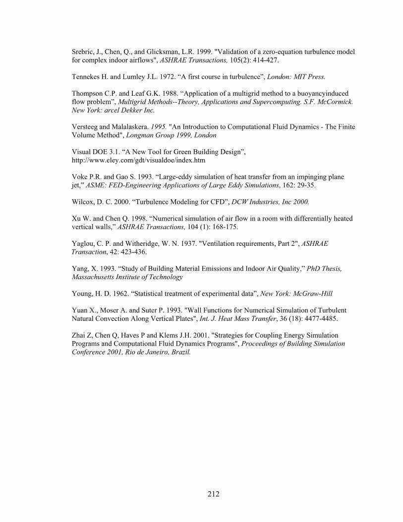
212

Srebric, J., Chen, Q., and Glicksman, L.R. 1999. "Validation of a zero-equation turbulence model for complex indoor airflows", ASHRAE Transactions, 105(2): 414-427. Tennekes H. and Lumley J.L. 1972. “A first course in turbulence”, London: MIT Press. Thompson C.P. and Leaf G.K. 1988. “Application of a multigrid method to a buoyancyinduced flow problem”, Multigrid Methods--Theory, Applications and Supercomputing. S.F. McCormick. New York: arcel Dekker Inc. Versteeg and Malalaskera. 1995. "An Introduction to Computational Fluid Dynamics - The Finite Volume Method", Longman Group 1999, London Visual DOE 3.1. “A New Tool for Green Building Design”, http://www.eley.com/gdt/visualdoe/index.htm Voke P.R. and Gao S. 1993. “Large-eddy simulation of heat transfer from an impinging plane jet,” ASME: FED-Engineering Applications of Large Eddy Simulations, 162: 29-35. Wilcox, D. C. 2000. “Turbulence Modeling for CFD”, DCW Industries, Inc 2000. Xu W. and Chen Q. 1998. “Numerical simulation of air flow in a room with differentially heated vertical walls,” ASHRAE Transactions, 104 (1): 168-175. Yaglou, C. P. and Witheridge, W. N. 1937. "Ventilation requirements, Part 2", ASHRAE Transaction, 42: 423-436. Young, H. D. 1962. “Statistical treatment of experimental data”, New York: McGraw-Hill Yuan, X., Chen, Q. and Glicksman, L. R. 1998. A critical review of displacement ventilation,

Energy and Building. ASHRAE Transaction, Vol. 104, part 1A: 78-90. Yuan X., Moser A. and Suter P. 1993. "Wall Functions for Numerical Simulation of Turbulent Natural Convection Along Vertical Plates", Int. J. Heat Mass Transfer, 36 (18): 4477-4485. Zhai Z, Chen Q, Haves P and Klems J.H. 2001. "Strategies for Coupling Energy Simulation Programs and Computational Fluid Dynamics Programs", Proceedings of Building Simulation Conference 2001, Rio de Janeiro, Brazil.

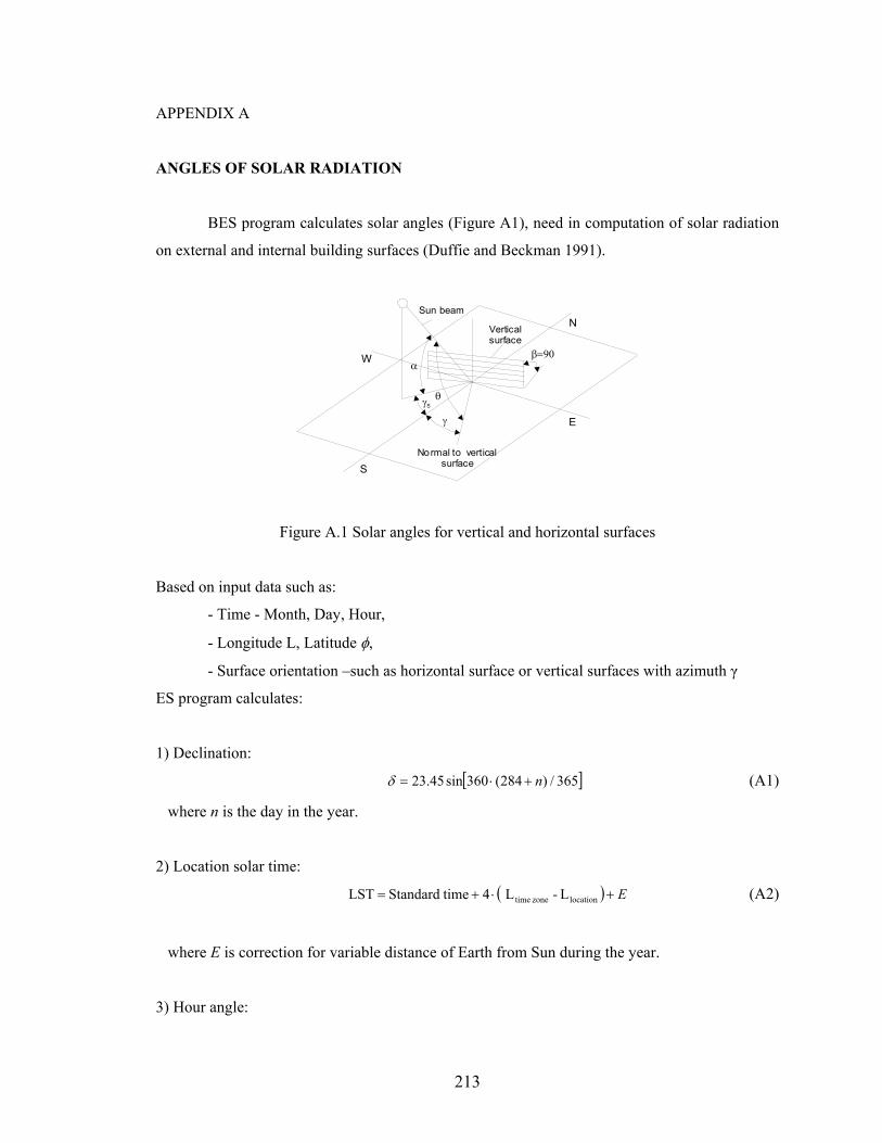
213

APPENDIX A

ANGLES OF SOLAR RADIATION

BES program calculates solar angles (Figure A1), need in computation of solar radiation

on external and internal building surfaces (Duffie and Beckman 1991).

Vertical surface

Normal to verticalsurface

γ

θ

α

S

E

NSun beam

W β=90

γS

Figure A.1 Solar angles for vertical and horizontal surfaces

Based on input data such as:

- Time - Month, Day, Hour,

- Longitude L, Latitude φ,

- Surface orientation –such as horizontal surface or vertical surfaces with azimuth γ

ES program calculates:

1) Declination:

[ ]365/)284(360sin45.23 n+⋅=δ (A1)

where n is the day in the year.

2) Location solar time:

( ) E+⋅+= locationzone time L-L 4 timeStandardLST (A2)

where E is correction for variable distance of Earth from Sun during the year.

3) Hour angle:

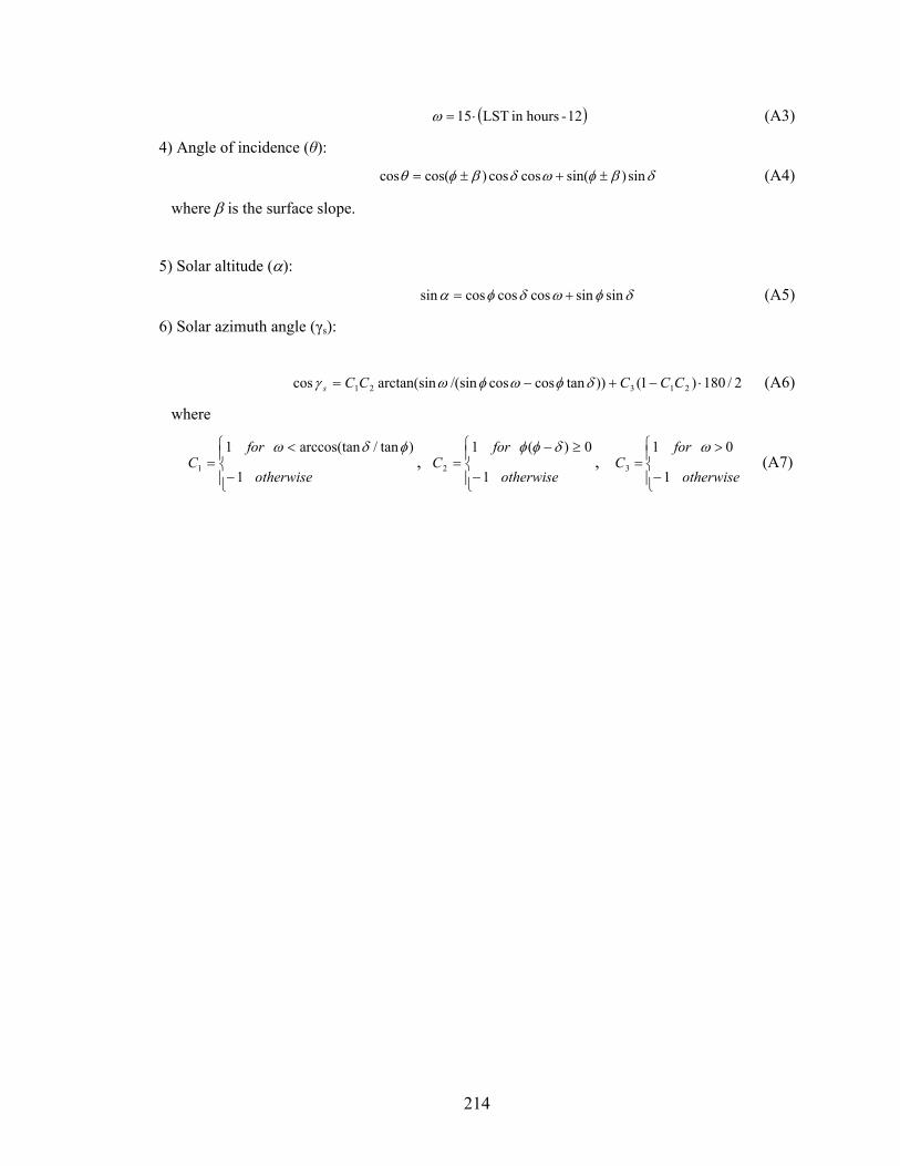
214

( )12 -hoursin LST15 ⋅=ω (A3)

4) Angle of incidence (θ):

δβφωδβφθ sin)sin(coscos)cos(cos ±+±= (A4)

where β is the surface slope.

5) Solar altitude (α):

δφωδφα sinsincoscoscossin += (A5)

6) Solar azimuth angle (γs):

2/180)1())tancoscos/(sinarctan(sincos 21321 ⋅−+−= CCCCCs δφωφωγ (A6)

where

−

<=

otherwise

forC

1

)tan/arccos(tan11

φδω,

−

≥−=

otherwise

forC

1

0)(12

δφφ,

−

>=

otherwise

forC

1

013

ω (A7)

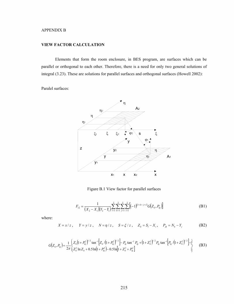
215

APPENDIX B

VIEW FACTOR CALCULATION

Elements that form the room enclosure, in BES program, are surfaces which can be

parallel or orthogonal to each other. Therefore, there is a need for only two general solutions of

integral (3.23). These are solutions for parallel surfaces and orthogonal surfaces (Howell 2002):

Paralel surfaces:

A2

ϕ1

s

y

A1

xx x2x1

y1

y2

y

ξ1 ξ2ξ ξ

η1

η

η2

η

ϕ2

z

η1

η

Figure B.1 View factor for parallel surfaces

( )( ) ( )( ) ( )[ ]∑∑∑∑= = = =

+++−−−

=2

1

2

1

2

1

2

1121212 ,11

l k j ikjli

ijkl PZGYYXX

F (B1)

where:

zxX /= , zyY /= , zN /η= , zS /ξ= , illi XSZ −= , jkjk YNP −= (B2)

( ) ( ) ( )[ ] ( ) ( )[ ]( ) [ ]

++−++

−+++−++=

−−−

2222

2/1212/1212/1212/12

1ln5.01ln5.0ln

1/tan1tan1/tan121,

kjlikjlili

likjkjlikjkjkjlikjlikjli

PZPZZ

ZPPZPPPZPZPZG

π (B3)

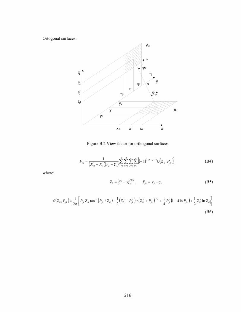
216

Ortogonal surfaces:

A2

A1

ϕ2

ϕ1

s

x

y

x x2x1

y1

y2

y

ξ1

ξ2

ξ

ξ

η1

ηη2

η

Figure B.2 View factor for orthogonal surfaces

( )( ) ( )( ) ( )[ ]∑∑∑∑= = = =

+++−−−

=2

1

2

1

2

1

2

1121212 ,11

l k j ijkli

ijkl PZGYYXX

F (B4)

where:

( ) 2/122illi xZ −= ξ , kjjk yP η−= (B5)

( ) ( ) ( ) ( ) ( )

+−++−−= −

lilijkjkjklijklilijklijkjkli ZZPPPZPZZPZPPZG ln21ln41

41ln

21/tan

21, 222/122221

π

(B6)

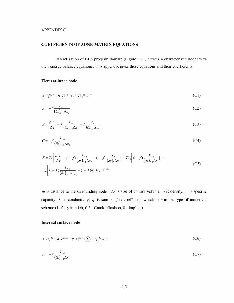
217

APPENDIX C

COEFFICIENTS OF ZONE-MATRIX EQUATIONS

Discretization of BES program domain (Figure 3.12) creates 4 characteristic nodes with

their energy balance equations. This appendix gives these equations and their coefficients.

Element-inner node

FTCTBTA III =⋅+⋅+⋅ ∆++

∆+∆+−

ττττττ11 (C1)

( ) II

I

xxkfA

∆−=

−

−

1

1

δ (C2)

( ) ( ) II

I

II

III

xxkf

xxkfcB

∆+

∆+

∆=

−

−

δδτρ

1

1 (C3)

( ) II

I

xxk

fC∆

−=+

+

1

1

δ (C4)

( ) ( ) ( )

( )ττττ

ττ

δ

δδδτρ

∆+

+

++

−

−−

−

−

+−+

∆

−

+

∆

−+

∆

−−∆

−−∆

=

qfqfxx

kfT

xxkfT

xxkf

xxkfcTF

II

II

II

II

II

I

II

IIII

)1()1(

)1()1()1(

1

11

1

11

1

1

(C5)

xδ is distance to the surrounding node , x∆ is size of control volume, ρ is density, c is specific

capacity, k is conductivity, q is source, f is coefficient which determines type of numerical

scheme (1- fully implicit, 0.5 - Crank-Nicolson, 0 - implicit).

Internal surface node

FTSTRTBTAn

iiSAII =⋅+⋅+⋅+⋅ ∑

=

∆+∆+∆+∆+−

1,1

ττττττττ (C6)

( ) II

I

xxk

fA∆

−=−

−

1

1

δ (C7)

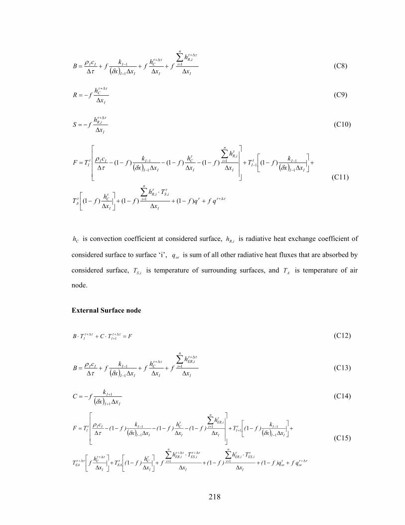
218

( ) I

n

iiR

I

C

II

III

x

hf

xhf

xxkfcB

∆+

∆+

∆+

∆=

∑=

∆+∆+

−

− 1,

1

1

ττττ

δτρ (C8)

I

C

xh

fR∆

−=∆+ ττ

(C9)

I

iR

xh

fS∆

−=∆+ ττ

, (C10)

( ) ( )

τττ

τττ

τ

τ

ττ

τ

δδτρ

∆+=

−

−−

=

−

−

+−+∆

⋅−+

∆

−

+

∆

−+

∆−−

∆−−

∆−−

∆=

∑

∑

qfqfx

Thf

xhfT

xxkfT

x

hf

xhf

xxkfcTF

I

n

iiSiR

I

CA

II

II

I

n

iiR

I

C

II

IIII

)1()1()1(

)1()1()1()1(

1,,

1

11

1,

1

1

(C11)

Ch is convection coefficient at considered surface, iRh , is radiative heat exchange coefficient of

considered surface to surface ‘i’, orq is sum of all other radiative heat fluxes that are absorbed by

considered surface, iST , is temperature of surrounding surfaces, and AT is temperature of air

node.

External Surface node

FTCTB II =⋅+⋅ ∆++

∆+ ττττ1 (C12)

( ) I

n

iiER

I

C

II

III

x

hf

xhf

xxkfcB

∆+

∆+

∆+

∆=

∑=

∆+∆+

−

− 1,

1

1

ττττ

δτρ (C13)

( ) II

I

xxkfC

∆−=

+

+

1

1

δ (C14)

( ) ( )

τττ

τττττττ

τττ

ττ

τ

ττ

τ

δδτρ

∆+==

∆+∆+∆+

∆+

−

−+

=

−

−

+−+∆

⋅−+

∆

⋅+

∆

−+

∆

+

∆

−+

∆−−

∆−−

∆−−

∆=

∑∑

∑

ororI

n

ii,ESi,ER

I

n

ii,ESi,ER

I

CEA

I

CEA

II

II

I

n

ii,ER

I

C

II

IIII

qfq)f(x

Th)f(

x

Thf

xh)f(T

xhfT

xxk)f(T

x

h)f(

xh)f(

xxk)f(cTF

11 1

1 111

11

1

11

1

1

1

(C15)

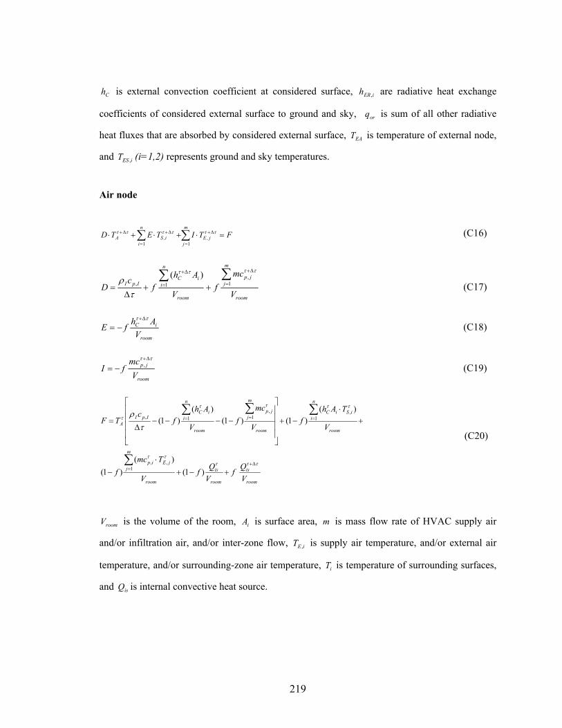
219

Ch is external convection coefficient at considered surface, iERh , are radiative heat exchange

coefficients of considered external surface to ground and sky, orq is sum of all other radiative

heat fluxes that are absorbed by considered external surface, EAT is temperature of external node,

and iEST , (i=1,2) represents ground and sky temperatures.

Air node

FTITETDm

jj,E

n

ii,SA =⋅+⋅+⋅ ∑∑

=

∆+

=

∆+∆+

11

ττττττ (C16)

room

m

jjp

room

n

iiC

IpI

V

mcf

V

Ahf

cD

∑∑=

∆+

=

∆+

++∆

= 1,

1,)( ττττ

τρ

(C17)

room

iC

VAhfE

ττ ∆+

−= (C18)

room

jp

Vmc

fIττ ∆+

−= , (C19)

room

is

room

is

room

m

jjEip

room

n

iiSiC

room

m

jjp

room

n

iiC

IpIA

VQf

VQf

V

Tmcf

V

TAhf

V

mcf

V

Ahf

cTF

τττττ

ττττ

τ

τρ

∆+=

===

+−+⋅

−

+⋅

−+

−−−−∆

=

∑

∑∑∑

)1()(

)1(

)()1()1(

)()1(

1,,

1,

1,

1,

(C20)

roomV is the volume of the room, iA is surface area, m is mass flow rate of HVAC supply air

and/or infiltration air, and/or inter-zone flow, iET , is supply air temperature, and/or external air

temperature, and/or surrounding-zone air temperature, iT is temperature of surrounding surfaces,

and isQ is internal convective heat source.

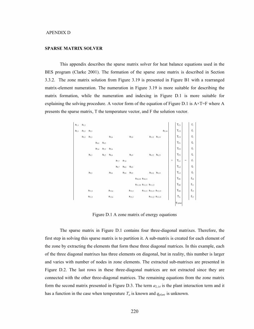
220

APENDIX D

SPARSE MATRIX SOLVER

This appendix describes the sparse matrix solver for heat balance equations used in the

BES program (Clarke 2001). The formation of the sparse zone matrix is described in Section

3.3.2. The zone matrix solution from Figure 3.19 is presented in Figure B1 with a rearranged

matrix-element numeration. The numeration in Figure 3.19 is more suitable for describing the

matrix formation, while the numeration and indexing in Figure D.1 is more suitable for

explaining the solving procedure. A vector form of the equation of Figure D.1 is A×T=F where A

presents the sparse matrix, T the temperature vector, and F the solution vector.

a1,1 a1,2 TC1 f1

a2,1 a2,2 a2,3 a2,14 TC2 f2

a3,2 a3,3 a3,6 a3,9 a3,12 a3,13 TC3 f3

a4,4 a4,5 TF1 f4

a5,4 a5,5 a5,6 TF2 f5

a6,3 a6,5 a6,6 a6,9 a6,12 a6,13 TF3 f6

a7,7 a7,8 × TL1 = f7

a8,7 a8,8 a8,9 TL2 f8

a9,3 a9,6 a9,8 a9,9 a9,12 a9,13 TL3 f9

a10,10 a10,11 TR1 f10

a11,10 a11,11 a11,12 TR2 f11

a12,3 a12,6 a12,3 a12,11 a12,12 a12,13 TR3 f12

a13,3 a13,6 a13,3 a13,12 a13,13 TA f13

q plant

Figure D.1 A zone matrix of energy equations

The sparse matrix in Figure D.1 contains four three-diagonal matrixes. Therefore, the

first step in solving this sparse matrix is to partition it. A sub-matrix is created for each element of

the zone by extracting the elements that form these three diagonal matrices. In this example, each

of the three diagonal matrixes has three elements on diagonal, but in reality, this number is larger

and varies with number of nodes in zone elements. The extracted sub-matrixes are presented in

Figure D.2. The last rows in these three-diagonal matrices are not extracted since they are

connected with the other three-diagonal matrices. The remaining equations from the zone matrix

form the second matrix presented in Figure D.3. The term a2,14 is the plant interaction term and it

has a function in the case when temperature Ta is known and qplant is unknown.

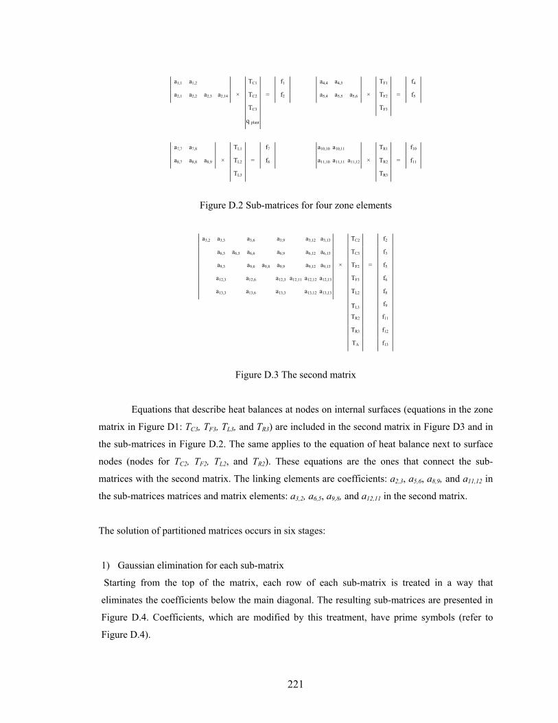
221

a1,1 a1,2 TC1 f1 a4,4 a4,5 TF1 f4

a2,1 a2,2 a2,3 a2,14 × TC2 = f2 a5,4 a5,5 a5,6 × TF2 = f5

TC3 TF3

q plant

a7,7 a7,8 TL1 f7 a10,10 a10,11 TR1 f10

a8,7 a8,8 a8,9 × TL2 = f8 a11,10 a11,11 a11,12 × TR2 = f11

TL3 TR3

Figure D.2 Sub-matrices for four zone elements

a3,2 a3,3 a3,6 a3,9 a3,12 a3,13 TC2 f2

a6,3 a6,5 a6,6 a6,9 a6,12 a6,13 TC3 f3

a9,3 a9,6 a9,8 a9,9 a9,12 a9,13 × TF2 = f5

a12,3 a12,6 a12,3 a12,11 a12,12 a12,13 TF3 f6

a13,3 a13,6 a13,3 a13,12 a13,13 TL2 f8

TL3 f9

TR2 f11

TR3 f12

TA f13

Figure D.3 The second matrix

Equations that describe heat balances at nodes on internal surfaces (equations in the zone

matrix in Figure D1: TC3, TF3, TL3, and TR3) are included in the second matrix in Figure D3 and in

the sub-matrices in Figure D.2. The same applies to the equation of heat balance next to surface

nodes (nodes for TC2, TF2, TL2, and TR2). These equations are the ones that connect the sub-

matrices with the second matrix. The linking elements are coefficients: a2,3, a5,6, a8,9, and a11,12 in

the sub-matrices matrices and matrix elements: a3,2, a6,5, a9,8, and a12,11 in the second matrix.

The solution of partitioned matrices occurs in six stages:

1) Gaussian elimination for each sub-matrix

Starting from the top of the matrix, each row of each sub-matrix is treated in a way that

eliminates the coefficients below the main diagonal. The resulting sub-matrices are presented in

Figure D.4. Coefficients, which are modified by this treatment, have prime symbols (refer to

Figure D.4).

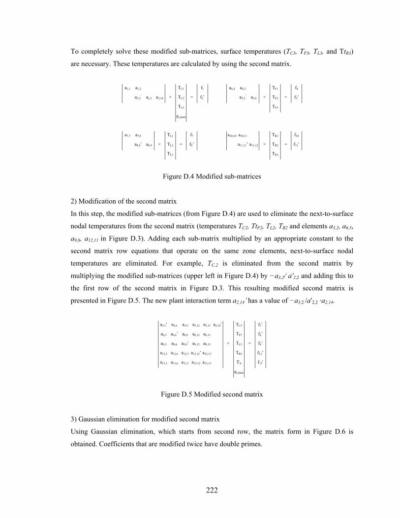
222

To completely solve these modified sub-matrices, surface temperatures (TC3, TF3, TL3, and TtR3)

are necessary. These temperatures are calculated by using the second matrix.

a1,1 a1,2 TC1 f1 a4,4 a4,5 TF1 f4

a2,2’ a2,3 a2,14 × TC2 = f2’ a5,5

’ a5,6 × TF2 = f5’

TC3 TF3

q plant

a7,7 a7,8 TL1 f7 a10,10 a10,11 TR1 f10

a8,8’ a8,9 × TL2 = f8’ a11,11’ a11,12 × TR2 = f11’

TL3 TR3

Figure D.4 Modified sub-matrices

2) Modification of the second matrix

In this step, the modified sub-matrices (from Figure D.4) are used to eliminate the next-to-surface

nodal temperatures from the second matrix (temperatures TC2, TtF2, TL2, TR2 and elements a3,2, a6,5,

a9,8, a12,11 in Figure D.3). Adding each sub-matrix multiplied by an appropriate constant to the

second matrix row equations that operate on the same zone elements, next-to-surface nodal

temperatures are eliminated. For example, TC,2 is eliminated from the second matrix by

multiplying the modified sub-matrices (upper left in Figure D.4) by −a3,2/ a′2,2 and adding this to

the first row of the second matrix in Figure D.3. This resulting modified second matrix is

presented in Figure D.5. The new plant interaction term a2,14’ has a value of −a3,2 /a′2,2 ·a2,14.

a3,3’ a3,6 a3,9 a3,12 a3,13 a2,14’ TC3 f3’

a6,3 a6,6’ a6,9 a6,12 a6,13 TF3 f6’

a9,3 a9,6 a9,9’ a9,12 a9,13 × TL3 = f9’

a12,3 a12,6 a12,3 a12,12’ a12,13 TR3 f12’

a13,3 a13,6 a13,3 a13,12 a13,13 TA f13'

q plant

Figure D.5 Modified second matrix

3) Gaussian elimination for modified second matrix

Using Gaussian elimination, which starts from second row, the matrix form in Figure D.6 is

obtained. Coefficients that are modified twice have double primes.

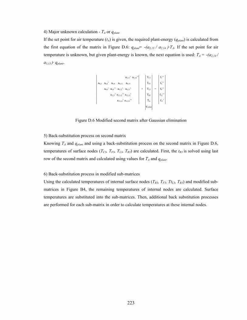
223

4) Major unknown calculation - TA or qplant

If the set point for air temperature (tA) is given, the required plant-energy (qplant) is calculated from

the first equation of the matrix in Figure D.6: qplant= -(a3,13 / a2,14 )·TA. If the set point for air

temperature is unknown, but given plant-energy is known, the next equation is used: TA = -(a2,14 /

a3,13 )· qplant.

a3,13’ a2,14’’ TC3 f3’’

a6,3 a6,6’ a6,9 a6,12 a6,13 TF3 f6’’

a9,6’ a9,9’’ a9,12’ a9,13’ × TL3 = f9’’

a12,3’ a12,12’’ a12,13’ TR3 f12’’

a13,12’ a13,13’’ TA f13’

q plant

Figure D.6 Modified second matrix after Gaussian elimination

5) Back-substitution process on second matrix

Knowing TA and qplant and using a back-substitution process on the second matrix in Figure D.6,

temperatures of surface nodes (TC3, TF3, TL3, TR3) are calculated. First, the tR3 is solved using last

row of the second matrix and calculated using values for TA and qplant.

6) Back-substitution process in modified sub-matrices

Using the calculated temperatures of internal surface nodes (TR3, TF3, TtL3, TR3) and modified sub-

matrices in Figure B4, the remaining temperatures of internal nodes are calculated. Surface

temperatures are substituted into the sub-matrices. Then, additional back substitution processes

are performed for each sub-matrix in order to calculate temperatures at these internal nodes.

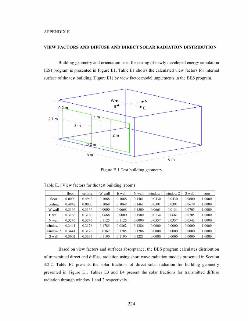
224

APPENDIX E

VIEW FACTORS AND DIFFUSE AND DIRECT SOLAR RADIATION DISTRIBUTION

Building geometry and orientation used for testing of newly developed energy simulation

(ES) program is presented in Figure E1. Table E1 shows the calculated view factors for internal

surface of the test building (Figure E1) by view factor model implements in the BES program.

6 m

2.7 m

3 m

8 m

0.2 m

0.2 m

1 m

2 m

SN

E

W

Figure E.1 Test building geometry

Table E.1 View factors for the test building (room)

floor ceiling W wall E wall N wall window 1 window 2 S wall sum floor 0.0000 0.4942 0.1068 0.1068 0.1461 0.0430 0.0430 0.0600 1.0000

ceiling 0.4942 0.0000 0.1068 0.1068 0.1461 0.0391 0.0391 0.0679 1.0000 W wall 0.3166 0.3166 0.0000 0.0668 0.1500 0.0661 0.0134 0.0705 1.0000 E wall 0.3166 0.3166 0.0668 0.0000 0.1500 0.0134 0.0661 0.0705 1.0000 N wall 0.3246 0.3246 0.1125 0.1125 0.0000 0.0357 0.0357 0.0543 1.0000

window 1 0.3441 0.3126 0.1785 0.0362 0.1286 0.0000 0.0000 0.0000 1.0000 window 2 0.3441 0.3126 0.0362 0.1785 0.1286 0.0000 0.0000 0.0000 1.0000

S wall 0.3002 0.3397 0.1190 0.1190 0.1221 0.0000 0.0000 0.0000 1.0000

Based on view factors and surfaces absorptance, the BES program calculates distribution

of transmitted direct and diffuse radiation using short wave radiation models presented in Section

3.2.2. Table E2 presents the solar fractions of direct solar radiation for building geometry

presented in Figure E1. Tables E3 and E4 present the solar fractions for transmitted diffuse

radiation through window 1 and 2 respectively.

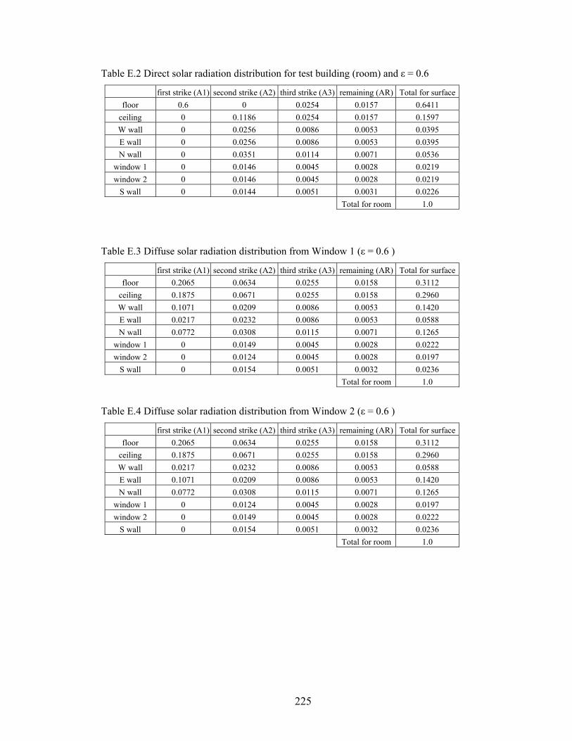
225

Table E.2 Direct solar radiation distribution for test building (room) and ε = 0.6

first strike (A1) second strike (A2) third strike (A3) remaining (AR) Total for surface floor 0.6 0 0.0254 0.0157 0.6411

ceiling 0 0.1186 0.0254 0.0157 0.1597 W wall 0 0.0256 0.0086 0.0053 0.0395 E wall 0 0.0256 0.0086 0.0053 0.0395 N wall 0 0.0351 0.0114 0.0071 0.0536

window 1 0 0.0146 0.0045 0.0028 0.0219 window 2 0 0.0146 0.0045 0.0028 0.0219

S wall 0 0.0144 0.0051 0.0031 0.0226 Total for room 1.0

Table E.3 Diffuse solar radiation distribution from Window 1 (ε = 0.6 )

first strike (A1) second strike (A2) third strike (A3) remaining (AR) Total for surface floor 0.2065 0.0634 0.0255 0.0158 0.3112

ceiling 0.1875 0.0671 0.0255 0.0158 0.2960 W wall 0.1071 0.0209 0.0086 0.0053 0.1420 E wall 0.0217 0.0232 0.0086 0.0053 0.0588 N wall 0.0772 0.0308 0.0115 0.0071 0.1265

window 1 0 0.0149 0.0045 0.0028 0.0222 window 2 0 0.0124 0.0045 0.0028 0.0197

S wall 0 0.0154 0.0051 0.0032 0.0236 Total for room 1.0

Table E.4 Diffuse solar radiation distribution from Window 2 (ε = 0.6 )

first strike (A1) second strike (A2) third strike (A3) remaining (AR) Total for surface floor 0.2065 0.0634 0.0255 0.0158 0.3112

ceiling 0.1875 0.0671 0.0255 0.0158 0.2960 W wall 0.0217 0.0232 0.0086 0.0053 0.0588 E wall 0.1071 0.0209 0.0086 0.0053 0.1420 N wall 0.0772 0.0308 0.0115 0.0071 0.1265

window 1 0 0.0124 0.0045 0.0028 0.0197 window 2 0 0.0149 0.0045 0.0028 0.0222

S wall 0 0.0154 0.0051 0.0032 0.0236 Total for room 1.0

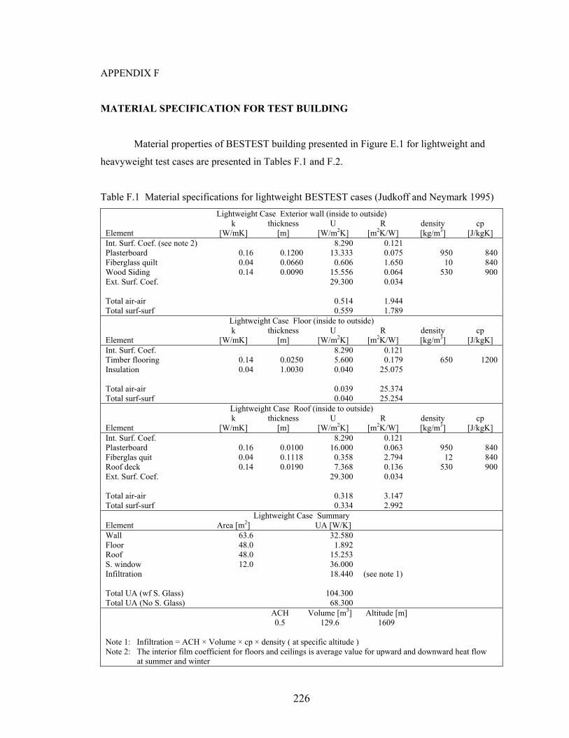
226

APPENDIX F

MATERIAL SPECIFICATION FOR TEST BUILDING

Material properties of BESTEST building presented in Figure E.1 for lightweight and

heavyweight test cases are presented in Tables F.1 and F.2.

Table F.1 Material specifications for lightweight BESTEST cases (Judkoff and Neymark 1995) Lightweight Case Exterior wall (inside to outside)

k thickness U R density cp Element [W/mK] [m] [W/m2K] [m2K/W] [kg/m3] [J/kgK] Int. Surf. Coef. (see note 2) 8.290 0.121 Plasterboard 0.16 0.1200 13.333 0.075 950 840 Fiberglass quilt 0.04 0.0660 0.606 1.650 10 840 Wood Siding 0.14 0.0090 15.556 0.064 530 900 Ext. Surf. Coef. 29.300 0.034 Total air-air 0.514 1.944 Total surf-surf 0.559 1.789

Lightweight Case Floor (inside to outside) k thickness U R density cp Element [W/mK] [m] [W/m2K] [m2K/W] [kg/m3] [J/kgK] Int. Surf. Coef. 8.290 0.121 Timber flooring 0.14 0.0250 5.600 0.179 650 1200 Insulation 0.04 1.0030 0.040 25.075 Total air-air 0.039 25.374 Total surf-surf 0.040 25.254

Lightweight Case Roof (inside to outside) k thickness U R density cp Element [W/mK] [m] [W/m2K] [m2K/W] [kg/m3] [J/kgK] Int. Surf. Coef. 8.290 0.121 Plasterboard 0.16 0.0100 16.000 0.063 950 840 Fiberglas quit 0.04 0.1118 0.358 2.794 12 840 Roof deck 0.14 0.0190 7.368 0.136 530 900 Ext. Surf. Coef. 29.300 0.034 Total air-air 0.318 3.147 Total surf-surf 0.334 2.992

Lightweight Case Summary Element Area [m2] UA [W/K] Wall 63.6 32.580 Floor 48.0 1.892 Roof 48.0 15.253 S. window 12.0 36.000 Infiltration 18.440 (see note 1) Total UA (wf S. Glass) 104.300 Total UA (No S. Glass) 68.300 ACH Volume [m3] Altitude [m] 0.5 129.6 1609 Note 1: Infiltration = ACH × Volume × cp × density ( at specific altitude ) Note 2: The interior film coefficient for floors and ceilings is average value for upward and downward heat flow at summer and winter

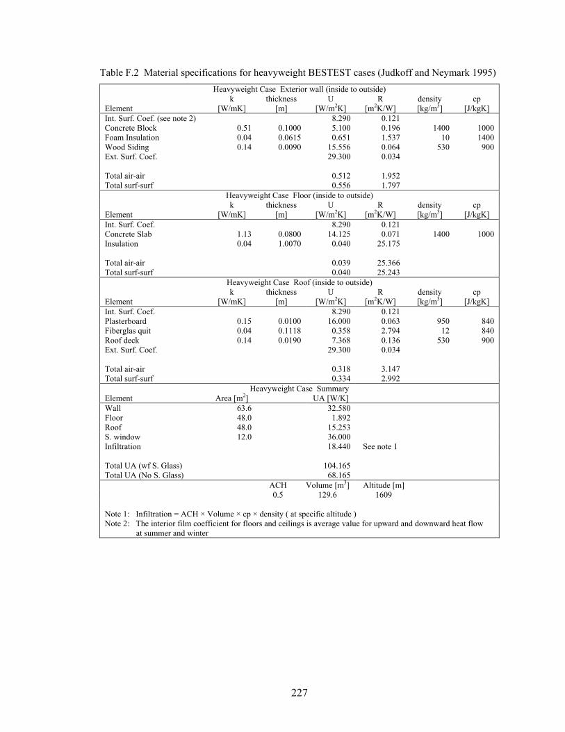
227

Table F.2 Material specifications for heavyweight BESTEST cases (Judkoff and Neymark 1995) Heavyweight Case Exterior wall (inside to outside)

k thickness U R density cp Element [W/mK] [m] [W/m2K] [m2K/W] [kg/m3] [J/kgK] Int. Surf. Coef. (see note 2) 8.290 0.121 Concrete Block 0.51 0.1000 5.100 0.196 1400 1000 Foam Insulation 0.04 0.0615 0.651 1.537 10 1400 Wood Siding 0.14 0.0090 15.556 0.064 530 900 Ext. Surf. Coef. 29.300 0.034 Total air-air 0.512 1.952 Total surf-surf 0.556 1.797

Heavyweight Case Floor (inside to outside) k thickness U R density cp Element [W/mK] [m] [W/m2K] [m2K/W] [kg/m3] [J/kgK] Int. Surf. Coef. 8.290 0.121 Concrete Slab 1.13 0.0800 14.125 0.071 1400 1000 Insulation 0.04 1.0070 0.040 25.175 Total air-air 0.039 25.366 Total surf-surf 0.040 25.243

Heavyweight Case Roof (inside to outside) k thickness U R density cp Element [W/mK] [m] [W/m2K] [m2K/W] [kg/m3] [J/kgK] Int. Surf. Coef. 8.290 0.121 Plasterboard 0.15 0.0100 16.000 0.063 950 840 Fiberglas quit 0.04 0.1118 0.358 2.794 12 840 Roof deck 0.14 0.0190 7.368 0.136 530 900 Ext. Surf. Coef. 29.300 0.034 Total air-air 0.318 3.147 Total surf-surf 0.334 2.992

Heavyweight Case Summary Element Area [m2] UA [W/K] Wall 63.6 32.580 Floor 48.0 1.892 Roof 48.0 15.253 S. window 12.0 36.000 Infiltration 18.440 See note 1 Total UA (wf S. Glass) 104.165 Total UA (No S. Glass) 68.165 ACH Volume [m3] Altitude [m] 0.5 129.6 1609 Note 1: Infiltration = ACH × Volume × cp × density ( at specific altitude ) Note 2: The interior film coefficient for floors and ceilings is average value for upward and downward heat flow at summer and winter

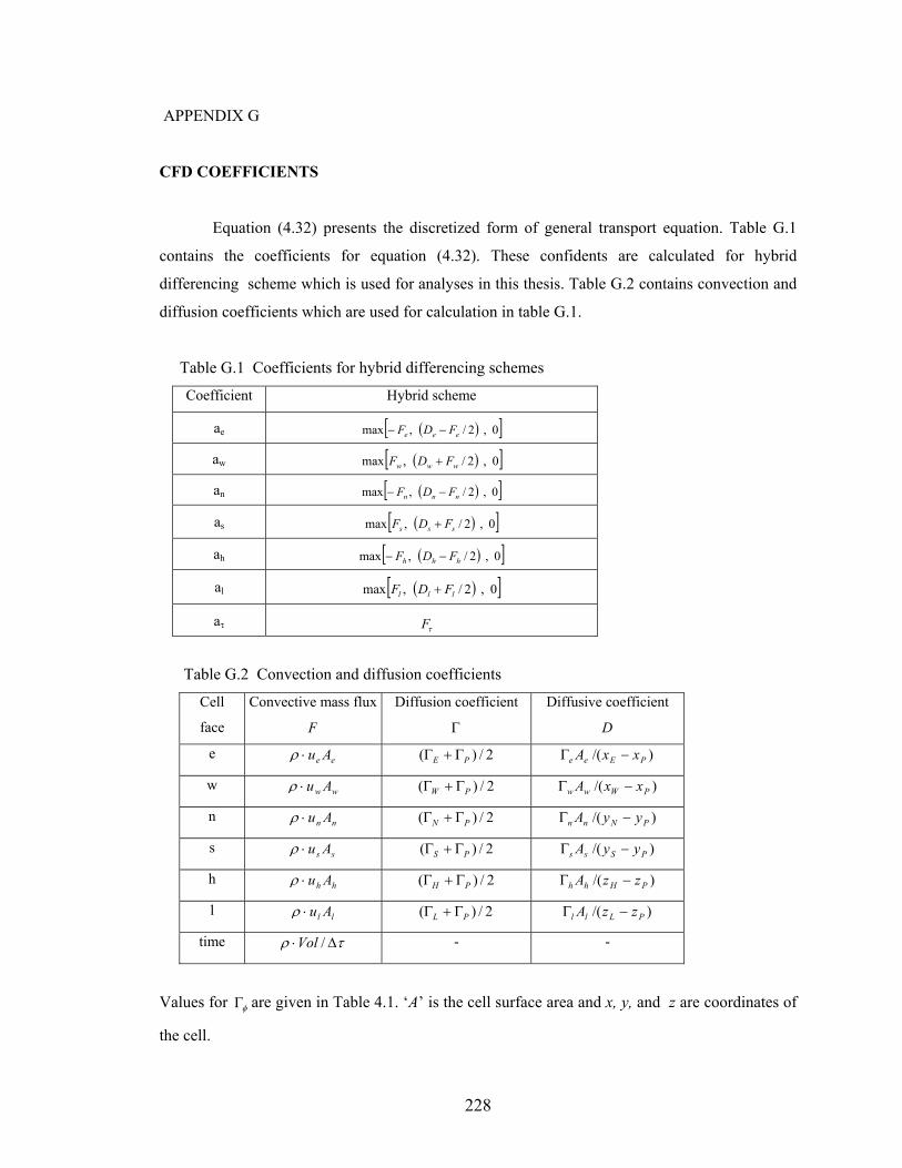
228

APPENDIX G

CFD COEFFICIENTS

Equation (4.32) presents the discretized form of general transport equation. Table G.1

contains the coefficients for equation (4.32). These confidents are calculated for hybrid

differencing scheme which is used for analyses in this thesis. Table G.2 contains convection and

diffusion coefficients which are used for calculation in table G.1.

Table G.1 Coefficients for hybrid differencing schemes

Coefficient Hybrid scheme

ae ( )[ ]0,2/,max eee FDF −−

aw ( )[ ]0,2/,max www FDF +

an ( )[ ]0,2/,max nnn FDF −−

as ( )[ ]0,2/,max sss FDF +

ah ( )[ ]0,2/,max hhh FDF −−

al ( )[ ]0,2/,max lll FDF +

aτ τF

Table G.2 Convection and diffusion coefficients

Cell

face

Convective mass flux

F

Diffusion coefficient

Γ

Diffusive coefficient

D

e ee Au⋅ρ 2/)( PE Γ+Γ )/( PEee xxA −Γ

w ww Au⋅ρ 2/)( PW Γ+Γ )/( PWww xxA −Γ

n nn Au⋅ρ 2/)( PN Γ+Γ )/( PNnn yyA −Γ

s ss Au⋅ρ 2/)( PS Γ+Γ )/( PSss yyA −Γ

h hh Au⋅ρ 2/)( PH Γ+Γ )/( PHhh zzA −Γ

l ll Au⋅ρ 2/)( PL Γ+Γ )/( PLll zzA −Γ

time τρ ∆⋅ /Vol - -

Values for φΓ are given in Table 4.1. ‘A’ is the cell surface area and x, y, and z are coordinates of

the cell.

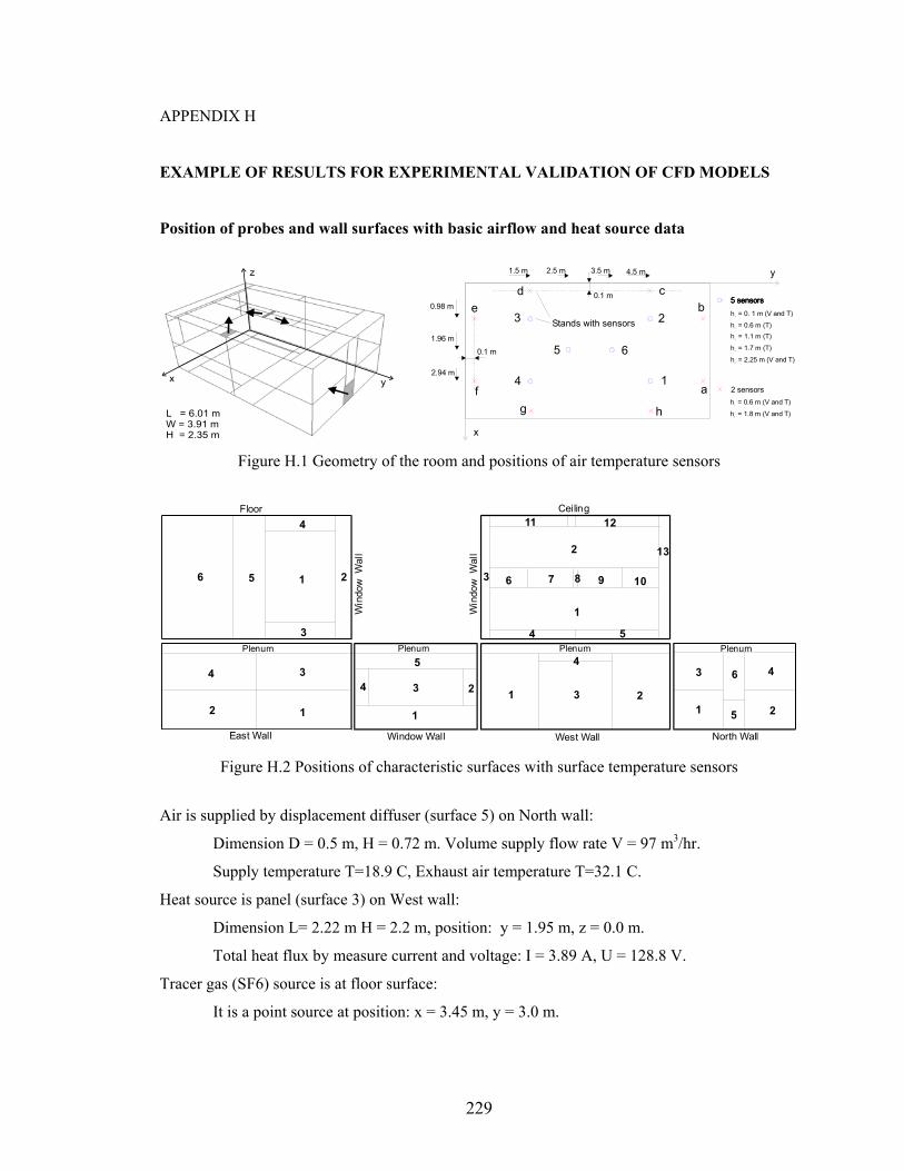
229

APPENDIX H

EXAMPLE OF RESULTS FOR EXPERIMENTAL VALIDATION OF CFD MODELS

Position of probes and wall surfaces with basic airflow and heat source data

yx

z

L = 6.01 mW = 3.91 mH = 2.35 m

5 sensors

2 sensors

5 sensors5 sensorsh = 0. 1 m (V and T)

1

h = 0.6 m 2

(T)h = 1.1 m

3(T)

h = 1.7 m 4

(T)

h = 2.25 m 5

(V and T)

h = 0.6 m 1

(V and T)

h = 1.8 m 2

(V and T)

Stands with sensors

x

y4.5 m1.5 m 2.5 m 3.5 m

0.98 m0.1 m

2.94 m

1.96 m

1

23

4

5 6

a

bcd

e

fg h

0.1 m

Figure H.1 Geometry of the room and positions of air temperature sensors

6 5 1

4

3

2 3 6 7 8 9 10

13

1211

54

1

2

Plenum

2

4

1

3

1

234

5

1 3 2

4

1 2

3 46

5

PlenumPlenumPlenum

Floor Ceiling

Window Wall North WallWest WallEast Wall

Win

dow

Wal

l

Win

dow

Wal

l

Figure H.2 Positions of characteristic surfaces with surface temperature sensors

Air is supplied by displacement diffuser (surface 5) on North wall:

Dimension D = 0.5 m, H = 0.72 m. Volume supply flow rate V = 97 m3/hr.

Supply temperature T=18.9 C, Exhaust air temperature T=32.1 C.

Heat source is panel (surface 3) on West wall:

Dimension L= 2.22 m H = 2.2 m, position: y = 1.95 m, z = 0.0 m.

Total heat flux by measure current and voltage: I = 3.89 A, U = 128.8 V.

Tracer gas (SF6) source is at floor surface:

It is a point source at position: x = 3.45 m, y = 3.0 m.

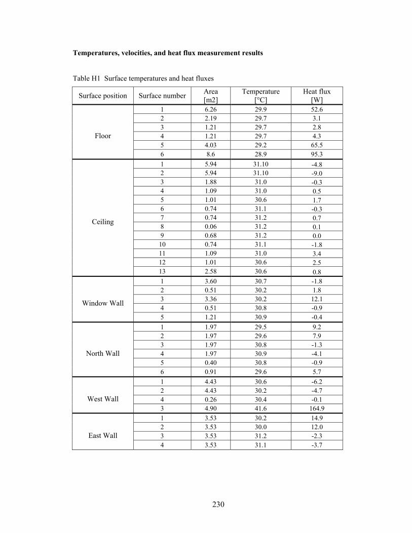
230

Temperatures, velocities, and heat flux measurement results

Table H1 Surface temperatures and heat fluxes

Surface position Surface number Area [m2]

Temperature [°C]

Heat flux [W]

1 6.26 29.9 52.6 2 2.19 29.7 3.1 3 1.21 29.7 2.8 4 1.21 29.7 4.3 5 4.03 29.2 65.5

Floor

6 8.6 28.9 95.3 1 5.94 31.10 -4.8 2 5.94 31.10 -9.0 3 1.88 31.0 -0.3 4 1.09 31.0 0.5 5 1.01 30.6 1.7 6 0.74 31.1 -0.3 7 0.74 31.2 0.7 8 0.06 31.2 0.1 9 0.68 31.2 0.0

10 0.74 31.1 -1.8 11 1.09 31.0 3.4 12 1.01 30.6 2.5

Ceiling

13 2.58 30.6 0.8 1 3.60 30.7 -1.8 2 0.51 30.2 1.8 3 3.36 30.2 12.1 4 0.51 30.8 -0.9

Window Wall

5 1.21 30.9 -0.4 1 1.97 29.5 9.2 2 1.97 29.6 7.9 3 1.97 30.8 -1.3 4 1.97 30.9 -4.1 5 0.40 30.8 -0.9

North Wall

6 0.91 29.6 5.7 1 4.43 30.6 -6.2 2 4.43 30.2 -4.7 4 0.26 30.4 -0.1 West Wall 3 4.90 41.6 164.9 1 3.53 30.2 14.9 2 3.53 30.0 12.0 3 3.53 31.2 -2.3 East Wall 4 3.53 31.1 -3.7

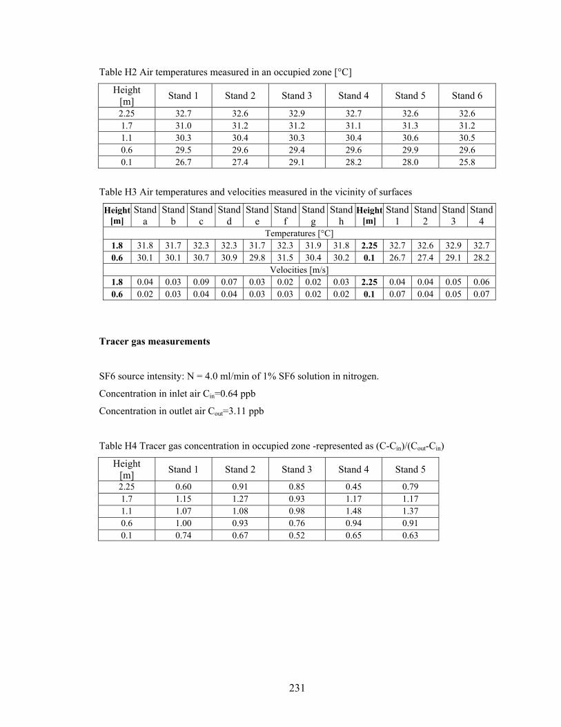
231

Table H2 Air temperatures measured in an occupied zone [°C]

Height [m] Stand 1 Stand 2 Stand 3 Stand 4 Stand 5 Stand 6

2.25 32.7 32.6 32.9 32.7 32.6 32.6 1.7 31.0 31.2 31.2 31.1 31.3 31.2 1.1 30.3 30.4 30.3 30.4 30.6 30.5 0.6 29.5 29.6 29.4 29.6 29.9 29.6 0.1 26.7 27.4 29.1 28.2 28.0 25.8

Table H3 Air temperatures and velocities measured in the vicinity of surfaces

Height [m]

Stand a

Stand b

Stand c

Stand d

Stand e

Stand f

Stand g

Stand h

Height [m]

Stand 1

Stand 2

Stand 3

Stand 4

Temperatures [°C] 1.8 31.8 31.7 32.3 32.3 31.7 32.3 31.9 31.8 2.25 32.7 32.6 32.9 32.7 0.6 30.1 30.1 30.7 30.9 29.8 31.5 30.4 30.2 0.1 26.7 27.4 29.1 28.2

Velocities [m/s] 1.8 0.04 0.03 0.09 0.07 0.03 0.02 0.02 0.03 2.25 0.04 0.04 0.05 0.06 0.6 0.02 0.03 0.04 0.04 0.03 0.03 0.02 0.02 0.1 0.07 0.04 0.05 0.07

Tracer gas measurements

SF6 source intensity: N = 4.0 ml/min of 1% SF6 solution in nitrogen.

Concentration in inlet air Cin=0.64 ppb

Concentration in outlet air Cout=3.11 ppb

Table H4 Tracer gas concentration in occupied zone -represented as (C-Cin)/(Cout-Cin)

Height [m] Stand 1 Stand 2 Stand 3 Stand 4 Stand 5

2.25 0.60 0.91 0.85 0.45 0.79 1.7 1.15 1.27 0.93 1.17 1.17 1.1 1.07 1.08 0.98 1.48 1.37 0.6 1.00 0.93 0.76 0.94 0.91 0.1 0.74 0.67 0.52 0.65 0.63

Vita - Atila Novoselac

Education

• Ph.D. in Architectural Eng, 2005 Architectural Engineering Department, The Pennsylvania State University • M.S. in Mechanical Eng, 2000 Department of Mechanical Engineering, University of Belgrade, Serbia • B.S. in Mechanical Eng, 1994 Department of Mechanical Engineering, University of Belgrade, Serbia Work Experience

• Graduate Student Researcher, 2000 – 2004 Department of Architectural Engineering, The Pennsylvania State University

• Research and Teaching Assistant, 1997 – 2000 Thermal Sciences Group, Dept. of Mechanical Engineering, University of Belgrade, Serbia

• Project Designer, 1995 – 2000 (2 days/week) Energy Institute, Dept. of Mechanical Engineering, University of Belgrade, Serbia

• Research Assistant, 1995 - 1997 Energy Institute, Dept. of Mechanical Engineering, University of Belgrade, Serbia

Academic Honors and Awards

• Jack and Laraine Beiter Excellence Endowment in Architectural Engineering, Penn State University, 2004 • Gordon D. Kissinger Graduate Fellowship, Penn State University, 2003 • Dean's Fellowship for Graduate Students, Penn State University, 2001-2004 • Grant in Aid Fellowship for Graduate Students, ASHRAE, 2001 • Government Fellowship for Young Investigators, Yugoslavia, March 1995 - May 1997 Activities and Associations

• American Society of Heating, Refrigerating and Air-Conditioning Engineers (ASHRAE) • Member of ASHRAE TC5.3 (Room Air Distribution) • Penn State Architectural Engineering Graduate Student Association Publications

• Novoselac, A. and Srebric, J. 2003. "Comparison of Air Exchange Efficiency and Contaminant Removal Effectiveness as IAQ Indices", ASHRAE Transactions, paper KC-03-4-5.

• Novoselac, A. and Srebric, J. 2002. "A Critical Review on the Performance and Design of Combined Cooled Ceiling and Displacement Ventilation Systems," Energy and Buildings, 34 (5): 497-509.

• Novoselac, A. and Srebric, J. 2003. “Sensitivity Study of Parameters Influencing IAQ indices”, Proceedings of Ventilation 2003, Sapporo, Japan.

• Srebric, J. and Novoselac, A. 2002. . “Design of Low-Energy Cooling System by Using Coupled Energy Simulation and Computational Fluid Dynamics”, Proceedings of Roomvent 2002, Copenhagen, Denmark.

• Novoselac, A. and Srebric, J. 2002. “Influence of Different Pollutant Sources on Selection of Ventilation System in Offices with Cooled Ceiling”, Proceedings of Indoor Air 2002, Monterey, California, USA.

• Marjanovic, L. Novoselac, A. 1997. “Radiator Valve's Influence on Hydrodynamic Performance of a Water Heating System”, Proceedings of Congress CLIMA 2000, Brussels.