Airline Emission Charges: Effects on Airfares, Service Quality, and Aircraft Design

by

Jan K. Brueckner Department of Economics

University of California, Irvine 3151 Social Science Plaza

Irvine, CA 92697 e-mail: jkbrueck@uci.edu

and

Anming Zhang

Sauder School of Business University of British Columbia

2053 Main Mall Vancouver, BC

Canada, V6T 1Z2 e-mail: anming.zhang@sauder.ubc.ca

January 2009

Abstract

This paper explores the effect of airline emissions charges on airfares, airline service quality, aircraft design features, and network structure, using a detailed and realistic theoretical model of competing duopoly airlines. These impacts are derived by analyzing the effects of an increase in the effective price of fuel, which is the path by which emissions charges will alter airline choices. The results show that emission charges will raise fares, reduce flight frequency, increase load factors, and raise aircraft fuel efficiency, while having no effect on aircraft size. Given that these adjustments occur in response to the treatment of an emissions externality that is currently unaddressed, they represent efficient changes that move society closer to a social optimum.

1

Airline Emission Charges: Effects on Airfares, Service Quality, and Aircraft Design

by

Jan K. Brueckner and Anming Zhang∗

1. Introduction

As concerns about global warming mount, policy makers have begun targeting emissions

from aircraft as a means of reducing the production of greenhouse gases. Most notably, the

European Union starting in 2012 will require airlines to hold emission permits in order to

operate. Each airline must hold a number of permits commensurate with the CO2 pollution

generated by its fleet, with permits acquired through a trading process following an initial,

partially free distribution among the carriers.1 This approach follows existing “cap-and-trade”

schemes applied to polluters in the industrial and energy sectors both in Europe and in the US

(see Forsyth, 2008, for details and further discussion).

The planned emission trading system generates a permit price that becomes part of an

airline’s cost structure. With the carrier’s required outlay on emissions permits varying in step

with its total fuel consumption, the permit price is effectively added to the price of fuel, even

though most of the permits will be freely distributed. Thus, the planned trading system can be

viewed as equivalent to a carbon-tax scheme applied to aviation, which would explicitly raise the

price of fuel. As a result, regardless of whether policy interventions to limit aviation emissions

follow the EU’s cap-and-trade approach or rely on taxation, they can all be depicted as policies

∗ We thank Michael Levine for stimulating comments. Any errors or shortcomings in the paper, however, are our responsibility. 1 As of late 2008, the EU’s intention was to freely distribute 85 percent of the total emission permits, with the remaining 15 percent auctioned. Movement to a 100 percent auction system is envisioned in later years. The permit distribution would cap emissions at 97 percent of the 2004-2006 level (see Wall, 2008).

2

that raise the fuel price paid by airlines. The effects of such policies thus operate in the same

direction as the impacts of a secular fuel-price increase unrelated to government intervention, as

occurred through mid-2008.

How will airlines respond to a policy-induced increase in the effective price of fuel?

What will happen to airfares? How will service quality, as reflected in flight frequencies and

load factors, change? How will aircraft design (fuel efficiency, seat capacity) evolve in response

to changes in the derived demands of airlines as fuel prices rise? Will the structure of airline

networks change? The purpose of the present paper is to answer these questions. The answers,

which are derived from a simple theoretical model, are important since they predict the detailed

response of a key, highly visible industry to a major government intervention in the fight against

global warming.

The paper builds on the approach used by Brueckner and Girvin (2008) in their analysis

of the impact of airport noise regulation. In the model, passengers value airline flight frequency

and dislike high load factors because of discomfort and the higher chance of being denied

boarding (bumped from a flight).2 Passengers choose between two competing airlines based on

these factors along with the fares they charge. Each airline incurs fuel cost, which depends on

aircraft fuel efficiency, as well as the capital cost of the aircraft in its fleet. This latter cost

depends on aircraft size (seating capacity) as well as fuel efficiency. With higher efficiency

requiring better engine technology as well as use of lighter materials, aircraft capital cost rises.

Even though both design features (size and efficiency) are set by the manufacturer, the airline is

portrayed as the ultimate decision-maker, with the manufacturer responding to its derived

2 While monetary compensation partly offsets the cost of denied boarding, some cost presumably remains for the typical bumped passenger.

3

demand for aircraft characteristics.3

A key issue in the analysis is the form of the function relating aircraft capital cost to size

and fuel efficiency, measured as fuel consumption per seat. While cost per seat is realistically

assumed to fall with aircraft size holding fuel efficiency constant, the interaction between fuel

efficiency and size in determining capital cost is less obvious a priori. The analysis imposes a

plausible general restriction on this interaction, which is satisfied by the specific functional form

that is adopted to facilitate the analysis. Although engineering data could, in principle, shed light

on the appropriateness of the adopted functional form, available data appear not to be rich

enough for this undertaking.4

The analysis in section 2 of the paper develops the model, deriving the airline profit

function. The key parameter in this function is the price per unit of fuel. Section 3 analyzes the

airline profit-maximization problem and carries out a comparative-static analysis. The model

solution is given by a nonlinear simultaneous equation system, but despite the system’s

complexity, comparative-static analysis is feasible and yields determinate fuel-price impacts.

Some of the comparative-static results are natural (for example, the fare rises with the fuel price),

but some findings are not predictable a priori. As a group, however, the comparative-static

results provide important information by showing how airline emission charges (either in the

3 To a certain extent, airlines can also affect average aircraft characteristics through their decisions on retirement of the older, less fuel-efficient planes in their fleets, and through fleet deployment/operations decisions with respect to aircraft size. 4 Data from the Boeing and Airbus websites (www.boeing.com and www.airbus.com) do indicate fuel-efficiency, measured as gallons consumed per seat mile, for various aircraft types. The numbers are 0.0171 for a 1988-vintage Airbus A320, 0.0139 for a 1998-vintage Boeing 737-800, 0.0166 for a 1998-vintage Boeing 777-300, 0.0180 for a 1995-vintage Airbus A340-600, and 0.0167 for a 2008-vintage Boeing 747-8. The values for the large aircraft (the last three) are similar, while the 737-800 value, which is from a smaller aircraft of a comparable vintage, is lower. Discounting the A320 value (which is similar to that for the larger aircraft) as reflecting the earlier 1988 vintage, the numbers suggest that the chosen level of fuel-efficiency is higher for smaller aircraft. While these numbers are revealing, exploring the relationship between capital cost and aircraft size and fuel efficiency would require additional data on aircraft selling prices. Since sales usually occur below list prices at values that are not publicly revealed, acquisition of price data is problematic. But even if such data were available, the small number of different existing aircraft types would probably not yield enough data points to estimate, using regression analysis, the desired relationship (this exercise, were it possible, would involve regressing price on fuel efficiency and size).

4

form of a price for emission permits or carbon tax) are likely to affect airline decisions. The

derived fare and service-quality impacts also yield an expected negative impact on passengers,

whose utility from direct consumption falls. This loss is ameliorated, however, by environmental

improvements from reduced emissions, as seen in the brief efficiency analysis presented in

section 4.

The last part of the analysis, in section 5, investigates the effect of a higher fuel price on

airline network structure, reflected in the choice between hub-and-spoke and fully-connected

(point-to-point) networks. By concentrating passengers on fewer routes, a hub-and-spoke

network allows better exploitation of the economies from larger aircraft, but its greater trip

circuity has an offsetting effect on costs. The analysis investigates how this trade-off is affected

by a higher fuel price, reaching a conclusion that is interestingly ambiguous. Thus, according to

the model, airline emission charges need not systematically affect current network structures.

Section 6 offers some brief empirical evidence in support of the model’s predictions, and section

7 presents conclusions.

2. The Model

Consider a travel market connecting two cities, which is served by two competing

airlines. A main component of the cost of serving passengers is aircraft operating costs, which

consist of fuel cost and the leasing (or ownership) cost of aircraft. The fuel cost depends on

aircraft fuel efficiency, which is measured as fuel consumption per seat per flight hour, denoted

by the variable e . The aircraft leasing cost per hour flown, denoted ),( seg , depends on aircraft

seating capacity s , as well as on fuel efficiency. Since a more fuel-efficient plane (with a lower

e) is more expensive (requiring better engine technology, better design, and/or use of lighter

materials), while a larger plane also costs more, g is decreasing in e and increasing in s .

5

Economies of larger aircraft mean that sg / is decreasing in s , and since successive increases in

fuel efficiency (decreases in e ) are increasingly expensive, g is convex in e . Additionally, a

negative cross partial derivative might make sense, implying that increases in fuel efficiency are

harder to achieve in a larger plane. While the g function is most easily viewed as a pure capital

cost, it could also include crew costs per hour, which depend on the size of the aircraft.

Letting r denote the price per unit of fuel, the flight cost per hour is given by

),( segres + , where the first term gives fuel cost. Letting k be hours per flight, the cost of one

flight is then equal to ksegres )],([ + .5 With f flights operated and k being an increasing

function of distance d, the airline’s total cost is thus given by

)()],([ dksegresf + . (1)

Expression (1) indicates that the airline’s cost depends on trip length and the number of seats per

aircraft, two variables found by Swan and Adler (2006) to be the main factors affecting aircraft

costs. Swan and Adler (2006) further argue )(dk is a linear function with a positive intercept,

implying economies of “stage length” (flight distance): the cost per kilometer flown declines as

the number of kilometers flown increases.

The two airlines serving the market, referred to as firms 1 and 2, carry passenger volumes

of 1q and 2q , respectively.6 Each consumer makes one trip on either airline 1 or airline 2, so

that the total number of passengers in the market is fixed and normalized to 1 ( 121 =+ qq ).

5 It should be noted that this cost formulation requires fuel consumption per flight hour to be independent of the duration of a flight. This independence is plausible given that high fuel consumption during the take-off phase of the flight is offset by low consumption during the landing phase, so that average fuel consumption per hour during these two phases may approximately equal to consumption per hour during the longer cruise phase of the flight. In this case, fuel consumption per hour may be roughly invariant to total flight duration, even though the landing and takeoff phases account for a smaller share of total flight hours on longer flights. 6 Although the analysis focuses on a duopoly market, it extends immediately to the n-firm case. With an n-firm oligopoly, the ½ term in traffic q (see below) is replaced by 1/n. This change can be demonstrated by applying the approach of Brueckner (2008) to the current model. For a noncompetitive alternative in developing this type of model, see Girvin (2008).

6

While consumers could in principle choose not to travel, making the passenger volume elastic,

the model assumes that travel demand is strong enough to allow the no-travel option to be

ignored. The quantities 1q and 2q depend on the fares charged by the airlines, denoted 1p and

2p , and on the service qualities they provide.

One element of service quality is flight frequency, which determines the “frequency

delay” experienced by a passenger (the difference between the passenger’s preferred departure

time and nearest flight time). When using a particular airline, a passenger’s expected frequency

delay is inversely proportional to the airline’s flight frequency f, assuming the passenger’s

preferred departure times are random and uniformly distributed and that flights are equally

spaced.7 The passenger’s cost of frequency delay on airline i can then be written γ/fi, where γ is

a cost parameter common to all passengers.

Douglas and Miller (1974) argue that another type of delay, denoted “stochastic delay,”

arises through excess demand, which may lead to denial of boarding on a flight that is oversold

and thus an additional delay. Stochastic delay is affected by airline’s load factor, which equals

the percentage of its seats filled by passengers. Following Panzar (1979), the analysis assumes

that a passenger’s probability of being denied a seat, and hence stochastic delay, is proportional

to an airline’s load factor, denoted li for airline i. The cost of stochastic delay can then be written

λli, where λ is a common cost parameter. Gathering all these elements, the cost of flying on

airline 1 is then the sum of the fare and the two delay costs, equal to 111 / lfp λγ ++ , with an

analogous expression for airline 2.

7 Assuming flights are equally spaced over the day, represented by a circle of circumference T, and that a passenger’s preferred departure time is random and distributed uniformly across the circle, expected frequency delay equals T/4f.

7

An additional motivation for the appearance of the load factor in the passenger’s cost

expression is possible. While generating stochastic delay, a high load factor also imposes a cost

on the passenger arising from aircraft crowdedness and the resulting discomfort. This

interpretation of the load factor’s impact will be useful in the welfare analysis presented below.

Although passengers compare the costs of flying in choosing between airlines 1 and 2,

brand loyalty also affects the choice, as in Brueckner and Girvin (2008). Brand loyalty appears

as an extra additive term in the cost expression for airline 1, which is negative for passengers

preferring airline 1 and positive for passengers preferring airline 2. Assuming that this brand

loyalty term is uniformly distributed over the interval ],[ αα− , the number of passengers

preferring airline 1 can be shown to equal

⎟⎟⎠

⎞⎜⎜⎝

⎛−−++−−= 2

21

1211

121 l

fl

fppq λγλγ

α, (2)

while the demand for airline 2 is given by the analogous expression with the 1 and 2 subscripts

interchanged (see Brueckner and Girvin (2008)). Thus an increase in flight frequency by airline

1 will increase its demand while reducing airline 2’s demand, and an increase in the load factor

or the fare will have the opposite effect. Note that, when all three variables are equal across the

two airlines, each airline faces a demand of ½, exactly splitting the total number of passengers

with its competitor.

Analysis of this model using a general form for the capital cost function ),( seg is

inconclusive. To generate determinate results, the capital-cost function is assumed to take the

following specific form:

esseg εβ +

=),( , (3)

8

where β and ε are positive parameters. The functional form in (3) satisfies all the conditions

specified above. Using (3), (2) and (1), the profit of airline 1 can be written as

)(1

1111111 dk

essrefqp ⎟⎟⎠

⎞⎜⎜⎝

⎛ ++−=

εβπ

)()()/(

111

1

111 dk

efqdk

lerep βε

−⎟⎟⎠

⎞⎜⎜⎝

⎛ +−=

)(121)()/(

112

21

121

1

111 dk

efl

fl

fppdk

lerep βλγλγ

αε

−⎥⎦

⎤⎢⎣

⎡⎟⎟⎠

⎞⎜⎜⎝

⎛−−++−−⎟⎟

⎠

⎞⎜⎜⎝

⎛ +−= . (4)

Note that the equality 1111 qlsf = , which equates total occupied seats to passengers, is used to

eliminate 1s in the second line of (4). Given this equality, only two of the variables 1f , 1s and 1l

can be choice variables for the airline. As seen in (4), 1f and 1l from among this group are

treated as the choice variables, leaving 1s to be deduced from the relationship 1111 / lfqs = . Note

also from (4) that the carrier’s total cost has two parts: one is proportional to the number of

passengers carried 1q , while the other part, namely kef )/( 11β , does not vary with the number of

passengers.8

With the model specification now clear, it is useful to explain how the imposition of

airline emission charges can be represented by an increase in the fuel price. As indicated in the

introduction, the impact of emissions charges is viewed as increasing the effective price of fuel

regardless of whether an EU-style cap-and-trade system or a carbon tax is used (a similar point is

made by Forsyth, 2008). To understand this claim, let x denote the number of permits required

per unit of fuel consumed, so that the number of permits needed by an airline is given by xfsek.

8 It should be noted that the above formulation assumes that aircraft size and frequency can be smoothly adjusted to suit the size of the market. In reality, such decisions involve indivisibilities such as minimum aircraft sizes and minimum viable flight frequencies, which may constrain actual choices.

9

Letting the emission permit price be denoted z and the number of permits allocated to the airline

be denoted m, the term )( mxfsekz − would then be subtracted from profit. This expression gives

the outlay for the purchase of permits when the airline requires more than its allocation (when

)mxfsek > , or the revenue from the sale of permits when the airline has more than it can use

(when )mxfsek < . As can be seen by inspecting the first profit expression in (4), the fuel price

r would then be replaced by zxr + , with the constant zm also subtracted from the profit

expression. Similarly, with a carbon tax t per unit of fuel, the fuel price would be replaced by

tr + . In either case, therefore, the impact of airline emission charges may be assessed simply by

analyzing the impact of an increase in the fuel price.

A final point regarding the model setup concerns the assumption of a fixed total

passenger volume ( 121 =+ qq ). Since the imposition of airline emission charges would be

expected to reduce the total volume of air travel by increasing its cost relative to other goods,

reliance on a model where this volume is fixed is not ideal. However, when the current approach

is imbedded in a model with an elastic travel demand, the complexity of the resulting framework

makes it amenable only to numerical analysis. Such analysis, which could adopt the elastic-

demand setup of Brueckner (2008), might be an undertaking in future research.9 But the first

priority is to explore a model capable of generating analytical results, and the present paper

reflects this priority despite the limitation of a fixed passenger volume.10

9 Brueckner and Flores-Fillol (2007) analyze a related model where the passenger volume is elastic, but Brueckner’s (2008) framework is more tractable. 10 This limitation was also present in the Brueckner and Girvin’s (2008) analysis of noise mitigation policies, which raise the fare but leave total passenger volume unchanged in their model.

10

3. Profit Maximization and Comparative Statics

This section analyzes the profit-maximization problem and carries out comparative-static

analysis. Consider the decisions faced by airline 1, which chooses 1p , 1e , 1f and 1l to maximize

profit. Using the profit function (4), airline 1’s first-order conditions can be written

(suppressing, hereinafter, the d argument of k(d)):

01)/(

1

1111

1

1 =⎟⎠⎞

⎜⎝⎛−⎟⎟⎠

⎞⎜⎜⎝

⎛ +−+=

∂∂

αεπ

kl

erepq

p (5)

0)/(21

111

21

1

1 =+−

−=∂∂

ekfkq

ler

eβεπ (6)

0)/(

12

11

111

1

1 =−⎟⎟⎠

⎞⎜⎜⎝

⎛ +−=

∂∂

ek

fk

lere

pf

βαγεπ (7)

.0)/()/(

1

1112

1

111

1

1 =⎟⎠⎞

⎜⎝⎛−⎟⎟⎠

⎞⎜⎜⎝

⎛ +−+

+=

∂∂

αλεεπ k

lerepk

lereq

l (8)

The first-order conditions for airline 2 are symmetric, and the second-order condition (positive

definiteness of the Hessian matrix of 1π ) is assumed to hold.

Given the symmetry of the model, the equilibrium values of ip , ie , if and il , i = 1,2,

will be symmetric across carriers, and each airline’s equilibrium traffic will equal ½. Imposing

symmetry in (5)-(8), substituting and rearranging, the following equations are obtained:

kl

erep )/(2

εα ++= (9)

rfle βε 22 +

= (10)

kefβγ

22 = (11)

11

.2

2 ke

relλ

ε+= (12)

The equilibrium, denoted ),,,( **** lfep , is the solution to equations (9)-(12).

To start the comparative-static analysis, let equation (10) be rewritten as flre βε 22 =− .

Squaring both sides, substituting (11) for the resulting 2f and (12) for 2l , and rearranging, the

equation can be rewritten as

;0)()2( 242 =Κ−⋅+Κ+⋅− εεε erer ,/2 λγβ≡Κ (13)

where Κ is a positive parameter. Applying the quadratic formula (viewing e2 as the unknown),

the solution for e is given by

( )[ ] ( )[ ] .2/)8(22/)(4)2()2(2/12/1

2222* rrrrre ΚΚ+±Κ+=Κ−−Κ+±Κ+= εεεεεε (14)

Equation (14) yields two positive solutions when Κ>ε , but one positive and one complex

solution when Κ<ε . In the latter case, the square root expression in the first part of (14) is

larger than the expression prior to the ± sign, making the entire expression (which is raised to

the ½ power) negative. To rule out the first multiple-solution case, Κ<ε is assumed to hold, so

that the unique (real) solution is given by the last expression in (14) with a plus sign prior to the

square root.

Equation (14) determines equilibrium *e as a function of the fuel price r and other

parameters ( λβγε ,,, ), written as )(* re after suppressing these latter arguments. Differentiating

(14) to find the effect of r yields

.02

**

<−=r

edrde (15)

Equation (15) indicates that an increase in the fuel price leads to a lower *e or, equivalently,

more fuel-efficient planes.

12

The comparative-static effects of the fuel price on the equilibrium values of the

remaining choice variables ),,( *** lfp are examined next. Once )(* re is determined, flight

frequency, by (11) equal to ,2/** kef βγ= is simply a function of parameters. Since *f

increases in ,*e which by (15) decreases in r, it follows that

,0*

<drdf (16)

so that an increase in the fuel price leads to a lower flight frequency.

For the effect on the load factor, rearranging (10) yields βε 2/])([ 2*** −= erlf .

Differentiating this equation yields

,0221)( *

***

=⎟⎟⎠

⎞⎜⎜⎝

⎛+= e

drder

drlfd

β (17)

where the second equality follows from (15). Expanding the derivative on the left-hand side of

(16) and rearranging then yields

0*

*

**

>−=drdf

fl

drdl , (18)

using (16). That is, an increase in the fuel price leads to a higher load factor. Furthermore, since

*** 2/1 lfs = , (17) implies

,0*

=drds (19)

so that a change in the fuel price does not affect aircraft size.

The fare in (9) depends on the fuel price both directly and indirectly via fuel efficiency

and the load factor. Capturing these channels, the impact of a higher fuel price can be

decomposed into four parts: (i) a positive direct effect (captured by the 0/ ** >lke expression

13

multiplying r*); (ii) a negative indirect effect via the use of more fuel-efficient planes, which

which leads to fuel savings (captured by */ lrk times drde /* ); (iii) a positive indirect effect via

the use of more fuel-efficient planes, which results in higher aircraft leasing cost (this effect

operates through e* in the denominator of the upper ratio term in (9)); and (iv) a negative indirect

effect via a higher load factor, which leads to downward pressure on per-passenger cost (this

effect operates through l* in the large ratio expression in (9)). Using (12) in (9), p* can be

rewritten as ** 2/ lp λα += , which allows the net effect of these four impacts to be captured

simply through the effect of the higher fuel price on l*. Thus, using (18),

,0*

>drdp (20)

so that the two positive effects above dominate the negative effects, leading to a higher fare in

response to an increase in the fuel price. Summarizing the above results yields

Proposition 1. An increase in r, or an equivalent imposition of airline emissions charges, will

lead to a higher fare, lower flight frequency, a higher load factor, more fuel-efficient aircraft,

and an unchanged aircraft size.

Given that both elements of airline service quality worsen, while the fare increases,

passengers are unambiguously worse off following the imposition of emission charges. In

addition, application of the envelope theorem to the profit expression in (4) shows that airline

profit falls in response to the imposition of charges (to the rise in r). Environmental benefits

from reduced emissions have not yet been considered, however, and this element will be added

in the next section.

A final comparative-static question concerns the effect of flight distance on the various

choice variables, and the answers are immediate. From (14), since e* is independent of k, fuel

14

efficiency is unaffected by flight distance. Equations (9), (11), and (12) then show that p*, f *,

and l* are respectively increasing, decreasing and increasing in k, so that the fare and load factor

rise, while frequency falls, when flight distance increases. Finally, from (10),

βε 2/])([ 2*** −= erlf and so **lf is unaffected by flight distance. Consequently, aircraft size

)2/1( *** lfs = is unaffected by flight distance.

4. Welfare Analysis

To carry out a welfare analysis, the damage from emissions must be considered along

with the interests of passengers and airlines. The treatment of passenger interests in the welfare

analysis can be greatly simplified if the costs associated with a higher load factor are attributed

entirely to aircraft crowding and discomfort rather than to stochastic delay. The reason is that

incorporation of the stochastic-delay element would require a more sophisticated analysis

involving random travel decisions. Under this restriction, total consumer utility can be

represented simply by consumption expenditure, equal to income minus travel costs, which are

in turn given by the airfare plus the costs of schedule delay and crowding. Brand loyalties also

affect utility, but they aggregate to a constant.

To compute social welfare W, consumer utility is added to airline profit, with emissions

damage then subtracted. Given symmetry and the unit mass of passengers, welfare can then be

written as

),2(/2 fesklfpyW μλγπ −−−−+= (21)

where y is passenger income and the last term represents emissions damage. Note that 2fesk

represents total fuel usage by the two airlines, while μ is a parameter that gives emissions

damage per unit of fuel burned (a linear relationship is assumed for simplicity). In the analysis

of (21), the fare cancels since it represents a transfer between passengers and the airlines.

15

Using a related model without any environmental components, Brueckner and Flores-

Fillol (2007) show that equilibrium is efficient in a situation when all potential passengers travel,

as in the current analysis. Adapting this result to the present context, the implication is that if μ

were equal to zero (eliminating any environmental concerns), then the equilibrium values of p, f,

e, and l would maximize the welfare expression in (21). The efficiency result in Brueckner and

Flores-Fillol’s model disappears, however, with the introduction of a travel/no-travel margin,

which makes the total quantity of passengers dependent on airline choices rather than fixed.

Efficiency would similarly disappear in the present model if it were modified to allow an elastic

travel demand, although (as explained above) this modification makes much of the analysis

intractable.

While equilibrium in the current fixed-passenger-volume framework is efficient when

when μ = 0, the equilibrium is inefficient when μ > 0. Emissions damage then arises, which

airlines ignore in their decisions, and achievement of efficiency requires charging for this

damage. Given the linearity of the damage function, this charge should be set equal to μ per unit

of fuel. Thus, μ is the proper value for the carbon tax t. In addition, it is easily shown that the

endogenous emissions-permit cost per unit of fuel emerging from the trading process (zx from

above) will also equal the damage parameter μ, provided that the total number of permits

distributed to the airlines is equal to the socially optimal emissions volume from (21).

The current situation, where airline emissions charges are absent, thus involves an

inefficient equilibrium. Since the effective fuel price is too low, the preceding analysis indicates

the directions of the divergence from efficiency. In particular, aircraft fuel efficiency is currently

too low, flight frequency is too high, and the load factor is too low, although aircraft size is

efficient. Emissions charges, by increasing the effective fuel price, would correct these

16

inefficiencies by raising aircraft fuel efficiency, reducing flight frequency, and raising the load

factor.

5. The Effect of Emission Charges on Airline Networks

This section investigates the effect of a higher fuel price on airline network structure,

reflected in the choice between hub-and-spoke (HS) and fully-connected (FC) networks.

Industry observers, policy makers and researchers have all speculated about the likely network

impacts of emissions charges, making such an inquiry useful.11 Although the analysis cannot

explicitly identify the optimal network configuration, the discussion investigates how emissions

charges (an increase in r) affect the relative profitability of HS and FC networks, which reveals

the direction of the incentive to switch configurations as r rises.

More specifically, the analysis is conducted using a three-node symmetric city layout,

with all the links equidistant and the three city-pair markets assumed to have the same demand.12

The three-city system is serviced by the two competing airlines, which both use an FC network

to serve the cities or both use an HS network (asymmetric network choices are ruled out). Under

the FC network, passengers in the three city-pair markets are carried by direct (nonstop) flights

on three routes. For a HS network, with one city serving as the hub, there are just two “spoke”

routes, which connect the two non-hub cities to the hub. While spoke passengers continue to

take direct flights, passengers traveling between the two non-hub cities must take two flights and

connect at the hub. As a result, on a given spoke route, both local traffic and connecting traffic is

carried. While this higher traffic volume allows airlines to capture economies of aircraft size,

thereby reducing costs, connecting passengers fly a longer distance than under the FC network,

11 For example, Albers, et al. (2009) argue that airlines may add an intermediate stop outside the EU on long international flights, so that the EU emissions charge only applies to the final short leg. 12 This three-city framework has been used by, among others, Brueckner (2004), Oum, et al. (1995), Zhang (1996) and Pels, et al. (2000).

17

which tends to raise costs.13 For simplicity and without loss of generality, connecting passengers

are assumed to pay the same fare as nonstop passengers.14

Given this setup, FC profit is just three times the single-route profit expression from (4).

The FC equilibrium, denoted ),,,( FCFCFCFC lfep , is then still the solution to equations (6)-(9).

In particular, FCe is determined by equation (14), and FCf is then determined by (11), FCl by

(12), FCp by (9), and FCFCFC lfs 2/1= .

In the HS case, however, revenue is pq3 , but costs are two times (1), or

ksegresf )],([2 + , given that there are only two routes under the HS network. Furthermore,

while the previous equality 1111 qlsf = applied in the FC case for airline 1, 1111 2qlsf = holds in the

HS case given that each spoke route carries passengers in two markets. As a result, HS profit for

airline 1 is

⎭⎬⎫

⎩⎨⎧

−⎥⎦

⎤⎢⎣

⎡ +−=

111

1

1111 3

2)/(343

ekfqk

lerepHS βεπ . (22)

That is, the HS profit equals three times a modified form of profit expression (4), where the ratio

term involving 1l is multiplied by 4/3 and the last term is multiplied by 2/3.

In the HS case, airline 1 maximizes profit (22) with respect to 1p , 1e , 1f and 1l , with

aircraft size 1s again the residual variable. Imposing symmetry in the resulting first-order 13 The ability to exploit the economies from larger aircraft when passenger volumes increase is an important force behind economies of traffic density. But, by allowing an increase in service quality, concentration of traffic in an HS network also affects demands in individual markets served by the network. Specifically, higher traffic allows an airline to increase flight frequency, and the improved convenience raises demand. On the other hand, higher traffic may allow the airline to raise its load factor, lowering per-passenger costs while at the same time reducing service quality, which tends to reverse the frequency-related demand increase. All of these forces are accounted for in the ensuing analysis. It should be noted that, while Oum, et al. (1995) explore the effects of these network complementarities on airlines’ competitive strategies in network choice, the present paper abstracts from network rivalry considerations. By assuming that the two airlines either both use a FC network or both use a HS network, the focus is instead on the effect of emissions charges on network choice at the industry level. 14 Without this restriction, the airlines will choose different fares for connecting and non-stop passengers. However, the equilibrium solutions for the remaining choice variables are nevertheless the same as when fares are constrained to be equal. Therefore, for expositional simplicity, the equal-fare assumption is imposed.

18

conditions and rearranging, the HS equilibrium, denoted ),,,( HSHSHSHS lfep , is the solution to

the following equations:

kl

erep

HS

HSHSHS

)/(34

2εα +

+= (23)

rlf

e HSHSHS

βε +=2 (24)

ke

f HSHS β

γ432 = (25)

.34 2

2 ke

relHS

HSHS λ

ε+= (26)

These equations differ from (9)-(12) by the appearance of the new multiplicative factors from

(22) in the appropriate positions. Tracing through the derivations, the new equation determining

HSe is

.0)]2/([)]2/(2[ 242 =Κ−⋅+Κ+⋅− εεε erer (27)

Note that (27) is the same as (13), which determines FCe , except that the Κ term in (14) is now

replaced by 2/Κ . To again ensure a unique solution to (27), 2/Κ<ε is assumed to hold,

leading to the solution15

( )[ ] .2/)2/)](2/(8[)2/(22/1

reHS ΚΚ++Κ+= εε (28)

Given HSe , HSf is then determined by (25), HSl by (26), HSp by (23) and HSHSHS lfs /1= .

From (28) and (14), it is easily seen that FCHS ee < , so that more fuel-efficient planes are

used under the HS network than under the FC network. The intuition behind this result is that,

since the average passenger flies farther, greater fuel economy is preferred. Furthermore, with

15 Note that this condition implies the previous condition .K<ε

19

Κ rising by a factor of 2 going from the HS to FC networks, it is easily seen that the e solution

rises by less than a factor of 2 , so that 2/ <HSFC ee .16 Thus,

.2 HSFCHS eee << (29)

Using (11), (25) and (29), it then follows that

.1232

32

2

2

<<=HS

FC

HS

FC

ee

ff (30)

Thus HSFC ff < , so that flight frequency is higher under the HS network than under the FC

network, a result also derived by Brueckner (2004) in a related monopoly model without fuel-

efficiency and load-factor choices. Furthermore, from (9) and (24),

βε 2/)( 2 −= FCFCFC relf , ./)( 2 βε−= HSHSHS relf

Dividing the two equations and using the equalities FCFCFC slf 2/1= and HSHSHS slf /1= yields

,12

2

>−−

=εε

HS

FC

FC

HS

rere

ss (31)

where the inequality follows from (29). Thus FCHS ss > holds, so that larger aircraft are

employed under the HS network than under the FC network. This is a sensible result, also

derived by Brueckner (2004): by concentrating passengers on fewer routes, a HS network allows

better exploitation of the economies from larger aircraft. Finally, the load factor comparison

between the two network types is ambiguous, an issue that is explored further in the appendix.

Summarizing yields

Proposition 2. Under the assumed network structure, the HS network has more fuel-efficient

aircraft than the FC network. In addition, aircraft are larger and flight frequency is higher in

the HS network than in the FC network. 16 Note that 2/ =HSFC ee if and only if 0=ε .

20

As indicated above, the main purpose of this section is to investigate how a higher fuel

price affects airline network structure, which is done by examining the impact of an increase in

r on the HS–FC profit differential.17 Applying the envelope theorem to (4) and (22), the

derivative of FCHS11 ππ − with respect to r , evaluated at the symmetric equilibrium, is given by

.2

34 kle

le

FC

FC

HS

HS⎟⎟⎠

⎞⎜⎜⎝

⎛+− (32)

An increase in r will favor a HS (FC) network, raising (lowering) the HS–FC profit differential,

when (32) is positive (negative). However, the sign of this expression is ambiguous. On the one

hand, more fuel efficient planes are used under the HS network ( FCHS ee < ), which tends to make

the expression positive. On the other hand, greater trip circuity under the HS network raises

costs relative to the FC network, as reflected in the difference between the 4 factor in the first

term of (32) and the 3 factor in the second term. This difference tends to make (32) negative. In

addition, as shown in the appendix, the load factors HSl and FCl in general take different

values.18

Denoting HSHSHS lkeF /2≡ and FCFCFC lkeF 2/3≡ , (32) is proportional to HSFC FF − .

However, it is easier to work with the ratio 22 / FCHS FF , which is less (greater) than 1 as HSFC FF −

is positive (negative). From (a1) in the appendix, this ratio equals

.34

2

2

3

3

2

2

εε

++

=HS

FC

FC

HS

FC

HS

rere

ee

FF (33)

17 Although the impact of a higher fuel price on the HS–FC profit differential is the focus of the present analysis, a straightforward extension shows that the same results apply to the HS–FC welfare differential. 18 Even if the two load factors were the same, the sign of (32) would be ambiguous. For instance, using

HSFC ee 2< from (29), the sign of (32) is the same as the sign of

]2)2/3(2[]/)2/3(2[)2/3(2 +−<+−=+− HSHSFCHSFCHS eeeeee . But since the last expression is positive, the inequality does not give the sign of the first expression and hence (32).

21

Both the first and last ratio terms on the right-hand side of (33) are greater than 1, but the second

term is less than 1. As a consequence, the relation between 2HSF and 2

FCF is unclear a priori.

However, substituting (14) and (28) into (33) yields

2/3

2

2

181211614

116181814

322

⎟⎟⎠

⎞⎜⎜⎝

⎛

++++++

++++++

=θθθθ

θθθθ

FC

HS

FF

; 5.00 <<θ , (34)

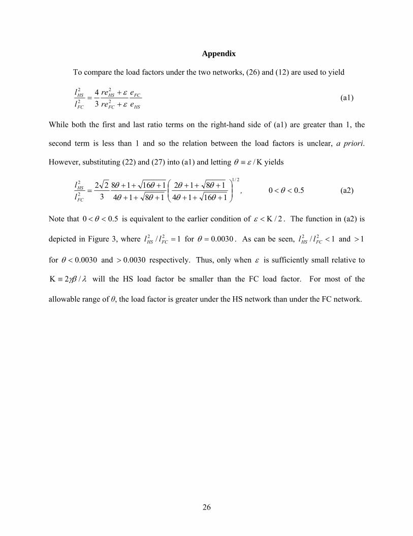
where Κ≡ /εθ . Setting the RHS of (34) to 1 results in a unique solution of 2025.0=Fθ .

Further, as depicted in Figure 1, 1)(/ 22 ><FCHS FF , as 2025.0)(><θ . Combining this result with

the above analysis, therefore, an increase in r will favor the HS (FC) network if

2025.0)(/ ><Kε .

Summarizing yields

Proposition 3. The imposition of emission charges (an increase in the fuel price) favors the HS

network when the cost parameter ε is small relative to λγβ /2≡K , with the FC network favored

otherwise.

Rearranging the inequality in Proposition 3 shows that imposition of airline emission

charges will favor the HS (FC) network if the cost ratio ε/β is small (large) relative to the demand

ratio γ/λ. Note that the inverse of the cost ratio is a measure of the economies of aircraft size

holding e fixed, being equal to the fixed cost β/e divided by the marginal seat cost, ε/e. Thus,

when size economies, as measured by β/ε, are sufficiently strong (when ε/β is sufficiently small),

an increase in the fuel price favors the HS network. By contrast, the demand ratio γ/λ is the ratio

of the cost of frequency delay and the cost associated with a higher load factor. When this ratio

is sufficiently large, an increase in the fuel price favors the FC network.

22

6. Empirical Evidence

Although a full empirical test of the model’s predictions is beyond the scope of the paper,

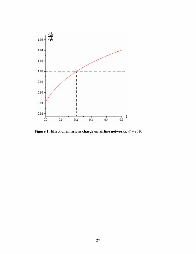
Figure 2 provides some suggestive evidence supporting some of the implications of the analysis.

The Figure shows four series over the 1993-2008 period: the aviation fuel price, revenue

passenger kilometers (RPK) per barrel of fuel (a measure of fuel productivity), non-fuel unit cost

(total non-fuel operating expenses divided by RPK), and the share of fuel cost in operating

expenses.19 The first three series are normalized by setting 1993 values equal to 100. The

numbers are based on aggregate data for all the world’s airlines offering scheduled services,

provided by the International Civil Aviation Organization (ICAO).

The aviation fuel price series shows dramatic escalation, rising almost seven-fold over

the period (from $16.79 per barrel in 1993 to $107.25 in 2008). This rise contrasts with the

slight, gradual decline in non-fuel expenses, measured on an RPK basis. The airlines’ response

to escalating fuel prices is documented in the remaining two series. Fuel productivity (RPK per

barrel of fuel) increases in step with the rising the fuel price, showing airline attempts to

conserve fuel as it becomes more expensive. This productivity increase presumably arises from

two separate adjustments portrayed in the model: (i) the improving fuel efficiency of new

aircraft, along with a shift in fleet composition toward such aircraft, and (ii) higher load factors.

Both adjustments lead to lower fuel usage per passenger kilometer, and together, they would

serve to moderate the price-driven increase in fuel expenses as a share of operating cost. As can

be seen in the fourth series, the rate of increase in this share declines after 2005, with the share

actually falling in 2008 (from 26 percent in 2007 to 24 percent in 2008) despite the large fuel-

cost spike in that year.

19 The data used in generating the four series are not available for the pre-1993 years.

23

It should be noted that imposition of emissions charges would lead to a less dramatic

increase in the effective price of fuel than the secular increase portrayed in Figure 2. A sense of

the relevant magnitude can be gained using data and calculations presented by Scheelhasse and

Grimme (2007). Consider their numbers for the low-cost carrier Ryanair, all of whose

operations are within the EU, making for an easy appraisal of the impact of EU-level charges.

Assuming that the price of a pollution permit (allowing the emission of one ton of CO2) equals

30€, Scheelhasse and Grimme’s computations show that the value of Ryanair’s required permits

would equal 2.65€ per passenger in 2008. Ryanair’s average fare is 44€, and assuming zero

profit and a 25 percent fuel share in costs (using the end-of-period value from Figure 2), the

implied fuel cost is 11€ per passenger. Since the permit cost per passenger is 24 percent of this

cost, emission charges can then be viewed as leading to a 24 percent increase in the effective

price of fuel. This increase is much smaller than the seven-fold rise over the 1993-2008 period

but appreciable nevertheless.

Note that, for a higher-cost carrier, this calculation would involve a higher fare but (given

such a carrier’s higher labor costs relative to Ryanair’s) a lower fuel share in total cost. The

resulting effective fuel-price increase would then be similar in magnitude to the 24 percent value

from above. Observe also that use of a fuel cost share smaller than the assumed 25 percent value

would raise the percentage increase in the effective fuel price associated with emissions charges.

Such a lower fuel cost share would be appropriate if the currently low fuel price persists.

7. Conclusion

This paper has explored the effect of airline emissions charges on airfares, airline service

quality, aircraft design features, and network structure, using a detailed and realistic theoretical

model of competing duopoly airlines. These impacts are derived by analyzing the effects of an

24

increase in the effective price of fuel, which is the path by which emissions charges will alter

airline choices. The results show that emission charges will raise fares, reduce flight frequency,

increase load factors, and raise aircraft fuel efficiency, while having no effect on aircraft size.

Given that these adjustments occur in response to the treatment of an emissions externality that is

currently unaddressed, they represent efficient changes that move society closer to a social

optimum.

Although these impacts are clear-cut, the effect of emission charges on the optimal

structure of airline networks is ambiguous. Under some parameter values, emission charges may

generate a shift away from current hub-and-spoke networks toward fully-connected, point-to-

point networks. But the profitability of HS networks could be reinforced by emission charges

under other parameter values.

The analysis has several limitations that could be addressed in future work. Most

importantly, the model assumes that the total volume of airline passengers is fixed and thus

unaffected by fuel prices and hence emission charges. More-realistic models that use the main

elements of the present approach but incorporate an elastic demand for travel could be analyzed,

but the resulting increase in complexity would necessitate use of numerical methods. The

analysis is also based on a special, though realistic, form for the key function relating aircraft

capital cost to seat capacity and fuel efficiency. Since some of the results (for example, the

invariance of aircraft size to fuel prices) may depend on use of this functional form, the effect of

adopting other specifications should be explored, perhaps numerically.

Airline emission charges are an important potential policy tool in the growing movement

to address global warming, and they affect a highly visible industry that serves an important,

affluent clientele. As a result, analysis of the impact of emission charges on airline decisions is a

25

high-priority undertaking, and this paper has offered a first step toward filling this need.

26

Appendix

To compare the load factors under the two networks, (26) and (12) are used to yield

HS

FC

FC

HS

FC

HS

ee

rere

ll

εε

++

= 2

2

2

2

34 (a1)

While both the first and last ratio terms on the right-hand side of (a1) are greater than 1, the

second term is less than 1 and so the relation between the load factors is unclear, a priori.

However, substituting (22) and (27) into (a1) and letting Κ≡ /εθ yields

2/1

2

2

116141812

181411618

322

⎟⎟⎠

⎞⎜⎜⎝

⎛

++++++

++++++

=θθθθ

θθθθ

FC

HS

ll

, 5.00 << θ (a2)

Note that 5.00 << θ is equivalent to the earlier condition of 2/Κ<ε . The function in (a2) is

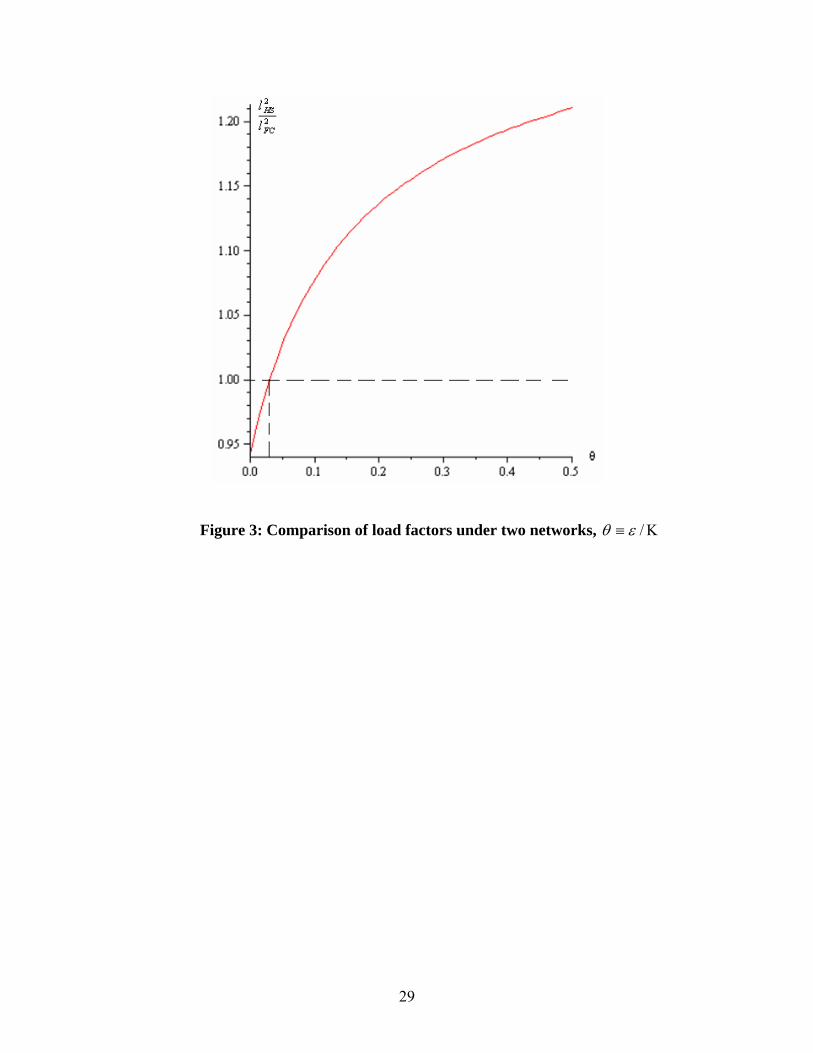
depicted in Figure 3, where 1/ 22 =FCHS ll for 0030.0=θ . As can be seen, 1/ 22 <FCHS ll and 1>

for 0030.0<θ and 0030.0> respectively. Thus, only when ε is sufficiently small relative to

λγβ /2≡Κ will the HS load factor be smaller than the FC load factor. For most of the

allowable range of θ, the load factor is greater under the HS network than under the FC network.

27

Figure 1: Effect of emissions charge on airline networks, Κ≡ /εθ

28

Figure 2: Fuel price, fuel productivity, share of fuel cost and non-fuel unit cost, 1993-2008 Notes: RPK = Revenue passenger kilometers; Fuel productivity = World RPK / barrel of fuel; Share of fuel cost = %

of fuel cost in total operating expenses; Non-fuel unit cost = Total non-fuel operating expenses / RPK; 2008F = forecast figures for 2008; Fuel price, fuel productivity and non-fuel unit cost are all indexed to 100 in 1993.

Source: Authors’ calculation based on the ICAO (International Civil Aviation Organization) database,

http://icaodata.com/.

29

Figure 3: Comparison of load factors under two networks, Κ≡ /εθ

30

References

Albers, S., J.-A. Buhne and H. Peters, 2009. Will the EU-ETS instigate airline network

reconfigurations? Journal of Air Transport Management 15, 1-6. Brueckner, J.K. and R. Flores-Fillol, 2007. Airline schedule competition, Review of Industrial

Organization 30, 161-177. Brueckner, J.K., 2004. Network structure and airline scheduling, Journal of Industrial

Economics 52, 291-312. Brueckner, J.K., 2008. Schedule competition revisited, Unpublished paper, Department of

Economics, UC Irvine. Brueckner, J.K. and R. Girvin, 2008. Airport noise regulation, airline service quality, and social

welfare, Transportation Research Part B 42, 19-37. Douglas, G.W. and J.C. Miller, 1974. Quality competition industry equilibrium, and efficiency

in the price constrained airline market, American Economic Review 64, 657-669. Forsyth, P., 2008. The impact of climate change policy on competition in the air transport

industry, Discussion paper 2008-18, OECD/ITF, Paris. Girvin, R., 2008. Airport noise regulation, airline service quality, and social welfare: The

monopoly case, Journal of Transport Economics and Policy, forthcoming. Oum, T.H., A. Zhang and Y. Zhang, 1995. Airline network rivalry, Canadian Journal of

Economics 28, 836-857. Panzar, J.C., 1979. Equilibrium and welfare in unregulated airline markets, American Economic

Review 69, 92-95. Pels, E., P. Nijkamp and P. Rietveld, 2000. A note on the optimality of airline networks,

Economics Letters 69, 429-434. Scheelhasse, J.D. and W.G. Grimme, 2007. Emissions trading for international aviation—an

estimation of the economic impact on selected European airlines, Journal of Air Transport Management 13, 253-263.

Swan, W.M. and N. Adler, 2006. Aircraft trip cost parameters: A function of stage length and

seat capacity, Transportation Research Part E 42, 105-115. Wall, R., 2008. Terms of trading, Aviation Week and Space Technology, October 6, p. 64.

31

Zhang, A., 1996. An analysis of fortress hubs in network-based markets, Journal of Transport Economics and Policy 30, 293-308.