NDER WORKING PAPERS SERIES

WHY ARE THERE SO MANY DIVIDED SENATE DELEGATIONS?

Alberto Alesina

Morris FiorinoHoward Rosenthal

Working Paper No. 3663

NATIONAL DOREAD OF EOONOMIO RESEAROM1050 Massachusetts Avenue

Oamnriage, MA 02138March 1991

Alesina and Rosenthal acknowledge financial support from NSFGrant SES0921441. This paper was written when Alesina was anOlin Fellow et the NREE and Rosenthal a Visiting Professor arW.I.T. Alesina gratefully acknowledges financial support fromthe Olin and Sloan foundations. We thank Keith Krehbiel, JohnLondregan, Eeith Poole, Kenneth Shepsie, end participants inseminars at Hoover Institution, Oarnegie-Nellon and University ofRochester for very useful coimsents end Gerald Oohen for excellentresearch assistance Any opinions expressed are those of theonthors and not those of the National Dnreau of Economic Raaeasch.

NDER Working Paper #3663March 1991

WHY ARE THERE SO MANY DIVIDED SENATE DELEGATIONS?

ABSTRACT

The last three decadea have witneased a sharp increase inthe number of states with spilt Senate deiegetions, featuring twosenators of different parties. In addition, there is evidencethat senators of different parties do not cluster in the middle:

they are genuinely polarized. We propose a model which explains

this phenomenon. Our argument builds upon the fact that when a

Sonnte election is held, there is already a sitting senator. If

thu voters care about the policy position of their state

delegation in each election, they may favor the candidate of the

party which is not holding the othuraeat. We show that, in

ganeral: (1) a candidate benefits if the non-running senator is

of thu opposing parry; (2) the more extreme the position uf the

non-running senator, the more extreme may be the position of the

opposing party candidate. Our 'opposite party advantage'

hypothesis is tested on a sample iacluding every Senate race from

1946 to 1986. After controlling for other important factors,

such as incumbency advantage, coattails end economic conditions,

we find reasonably strong evidence of the 'opposite party

advantage.'

Alherto Alesins Morris FiorinaHarvard Universicy, Harvard UniversityHEER, end OSPE

Haward EssenthalOarnugie-Mellon University

1. Introduction

Until recently the study of Congressional elections has generally aeant

the study of HAnse elections. Rut researchers have nuw begun to focus their

attentIon on Senate electicns. This increased interest probably has multiple

sources. To some extent, the political importance of recent Senate elections

draws our attention to them. The Republicans were able to capture the Senate

in 1980 and hold it until 1986, and their Senate majority was an irpurtant

component of the legislative successes of the Reagan administration. Another

basis of renewed interest in Senate elections undoubtedly stems from their

contrast with House elections. While the Republicans held the Senate from

1981—87, the House has remained safely in Democratic hands for thirty—five

years. Contrary to the expectations of the Framers, the electoral

responsiveness of the contemporary Senate is higher than that of the House

(Alford and Hibbing, 1989mb). Specifically, the advantages of incumbency in

contemporary House elections are almost overwhelming, hut incumbent fortunes

vary greatly in Senate elections.2 And while qualified, well—funded

challengers are a rarity in House elections (Jacobson, 1990, ch.4); Senate

incumbents seldom enjoy the luxury of unknown, under—funded challengers.

Occupying a position somewhere between presidential and House elections,

Senate elections seem to incorporate some of the major features of each Like

presidential nominees, Senate candidates are highly visible and their

campaigns heavily reliant on the mass media. Like Representatives, Senators

attempt to exploit the value of their incumbency, but it does not appear to

count for as much among the electorate. Issues and ideology are thought to be

mote important ln Senate elections than in House elections. But while

sometimes Senate races appear to hinge on major national issues, at other

times, the most parochial issues are thought to make the difference.3 And,

2

finally, one cannot ignore the importance of traditional partisanship despite

two deoedes of research on its weakening.4 Apparently analyses of Senate

elections must take into account the full range of variables that appear in

both presidential and House election studies.

While the new wave of research undoubtedly wll tell us a groat doal

about the specifics of Senate elections we should keep the larger picture in

mind. In particular, Senate elections show a number of interesting features

that pose explanatory challenges for the new research. In particular recent

reaeatch identifies two developments that appear to be both politically

consequential and theoretIcally puzzling. We will refer to these as the

"split state question," and the "polarization question."

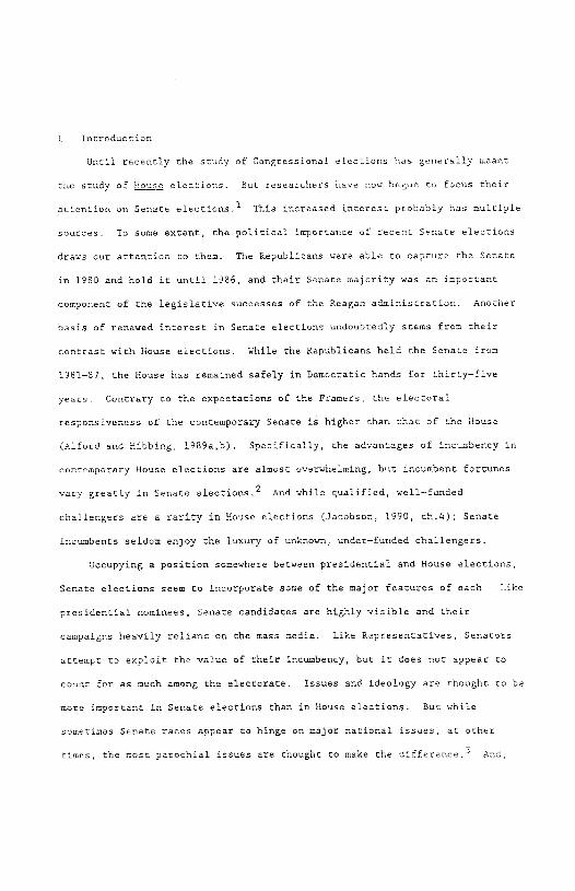
The split state question reflects the increase in the number of states

that divide their two Senate seats between the patties (Figure 1) . In recent

years state teptesentation in the Senate has been split as often as not, a

situation that oontrasts with the earlier historical tacord. In sutveying

that record Brady, Brody and Ferejohn (1989, pp. 3—4) observe

there is a dramatic rise in the number of split states begicning

in the 1960s. Prior to 19i0 (1918 on) theta were only fiva

instances of mixed state representation tising abovs 30 percent

while since 1960 no Congress has less than 30 percent and since

1966 the parcentage has nevet bean lower than 40 percent and has

been as high as 54 percent.

Poole and Rosenthal (1984b) point out that in the late seventies and early

eighties, the Senate had a distribution of delegations that was very nearly SO

Figure 1. States with Split Senatorial Delegations1946—1988

60

50

40

C

30

20

101946 1950 1954 1958 1962 1966 1970 1974 1978 1982 1986

1948 1952 1956 1960 1964 1968 1972 1976 1980 1984 1988Year

percent mixed, 25 percent Democratic, end 25 percent Republican, exactly what

cne would expect if every vcter came cc the polle end tossed a fair ccin tc

determine her Senete vcte. The facts are cbvicusly different, ac we are

challenged to show how individual behavior that is far from random generates

an aggregate outcome that is the epitome of randomness.5

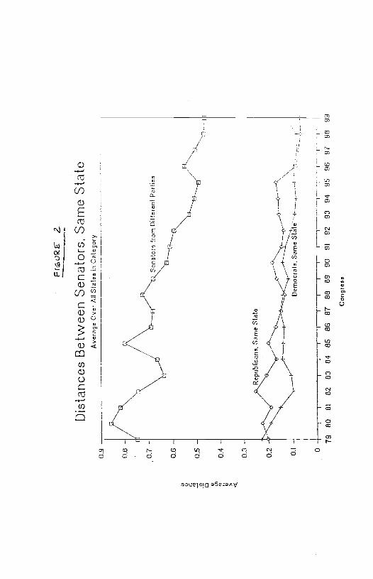
The polarization question reflects the grear ideological differences

between Democratic and Republican Senators (Figure 2). Poole and Rosenthal

(l984b) demonstrate that the Senate parties are not middle—of—the road, ma—too

parties; rather, they offer clear choices. Given decades of theorizing —

informal and formal that purports to identify centrist tendencies in two—

party electoral competitions, the polarization of the Senate patties

challenges us to identify the mechanism or forces that underlie it.7

Upon first observing split ststes one naturally thinks of the decline of

parties literature. And perhaps party decline provides a sufficient

explanation for split delegations If large numbers

of voters are not strongly moored to the parties, end if recruitment processes

characteristically generate and fund credible challengers in Senate races,

then "every race a toss—up" would appear to be the natural outcome.

Our difficulty wrh this argument arises when we view the split trend in

kflrionwitholgizarion, We would be more inclined to accept the

decline of parties explanation if all Senate candidates clustered around the

mid—point of the ideological spectrum. Then, wrh weak partisanship and

little to choose between on the issues, Senate rates would hinge on the

unpredictable distribution of attractive peraonalicfea, inspired campaign

commercials, ethics questions, local issues, and exogenous shocks. But the

candidates do not cluster in the middle. Instead, many states elect Th a

U

Ca a Ca U)

Ca a) >

pl2.

ocaE

a

Dis

tanc

es B

etw

een

Sen

ator

s, S

ame

Sta

te

Ave

rage

Ove

r A

lt S

tate

e in

Cat

egor

y 0.

9

0.0

0.7

0.6

0.5

0.4

0.3

0.2

Sam

e S

late

0

Dem

ocra

t a. S

ame

5ttë

±_.

___.

-I--

-'Th

79

80

81

82

83

84

85

86

87

88

89

90

91

92

93

94

95

06

97

90

99

Con

grea

e

liberal and a conservative. And the evidence is that when each comes up for

re—election, the electorate has a clear choice.8 Of course, if Senate

candidates were always equally polarized on the issues, then we might expecr

the seine outcome that would occur if they all converged to the median. But

then the question arises: why are Senate candidates so polarized?

In reflecting on Senate polarization most political scientists cite some

version of the "two constituencies thesis" (Huntington, 1950; Fiorina, 1974;

Brady, Brody end Ferejohn, 1989). In each state there are opposed groups of

activists who monitor government and participete in campaigns and consequently

hare their preferences weighted more heavily than those of average voters.

Empirical research suggests that such people have more extreme views than

ordinary voters and are highly polarized. Thus, candidates are drawn away

from the median by their need to please the activists. When the Democrats win

the Senator is more liberal than the state, whereas when the Republicans win

the Senator is more conservatfve,

Like most others we first viewed Senate polarization as indicative of the

two constituencies notion, But upon reflection the argument is clearly

insufficient. First, beginning with Downs (1957) three decades of theorizing

about electoral processes in two—party systems has repeatedly found strong

centrist tendencies. When equilibria exist they are typically some

generalized median. tTnen equilibrfa do not exist, minmax sets (Kramer, 1977);

stochastic solutions (Ferejohn, Fiorina, and Fackel, 1980), uncovered sets

(Shepsle and Welngast, 1984), and all other known theoretical models of

competitive processes suggest centrist outcomes seemingly at variance with the

polarization findings of Poole and Rosenthal (l984b). gven when candidates

are policy—oriented there are strong incentives to converge (Calvert, 1985).

More recently, however, Alesina (1988) showed that when votets learn candidate

ideology, the latter are not free to move in the policy space for credibility

reasons. In particular, extremists who sre known oe such, would not he

believed if they announced a moderate program. But although this recent work

explains why extremists may not be able to converge, we still need to explain

why centrist, moderate candidates do not enter and defeat relatively more

extreme competitors.

Some scholars also have tried to extend the two constituencies thesis to

explain the split trend (Brady, Brody, end Ferejohn, 1989). As with the

polarization question, we do not believe that the two constituencies thesis

can bear all of the explanatory weight, If one constituency is strong enough

to wn one election, why is it not strong enough to win the next one as well?

Surely, most state are not so closely divided that presidential coattails and

mid—term penalties are sufficient to swing each election, the former in favor

of one party, the latter in favor of the other. For the two constituencies

thesis to say anything about the increase in split states it must posit that

states are evenly divided politically, and additionally, identify some

consideration that systematically advantages first one constituency, then the

other.

We have identified such a consideration, one that contributes both to

split states and candidate polarization, Our argument builds on a key insight

that has not been taken account of in previous analyses:9 when a Senate

election is held, there is already a sitting Senator. If voters appreciate

that at any givsn time they are choosing the second member of a pair, rather

than making an unconditioned choice between two candidates, the nature of the

resulting electoral equilibrium is consistent with both the split state and

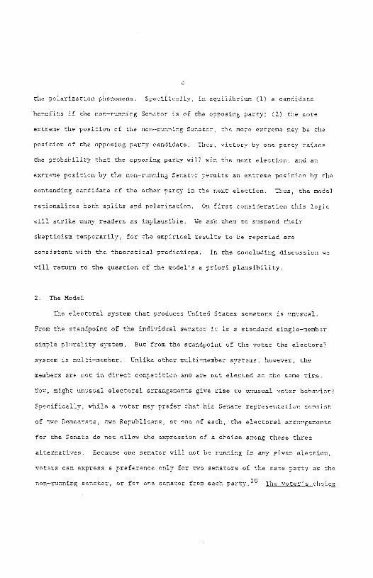
the polarization phenomena. Specifically, in equilibrium (1) a candidate

benefits if the non—running Senator is of the opposing party; (2) the more

extreme the position of the non—running Senator, the more extreme may be the

position of the opposing party candidate. Thus victory by one party raises

the probability that the opposing party will win the next election, and an

extreme position by the non—running Senator permits an extreme position by the

contending candidate of the other party in the next election. Thus the model

rationalizes both splits and polarization. On first consideration this logic

will strike many readers as implausible. We ask them to suspend their

skepticism temporarily, for the empirical results to be reported are

consistent with the theoretical predictions. In the concluding discussion we

will return to the question of the model's a priori plausibility.

2. The Model

The electoral system chat produces United States senators is unusual.

From the standpoint of the individual senator it is a standard single—member

simple plurality system. But from the standpoint of the voter the electoral

system is multi—member. Unlike ocher multi—member systems, however, the

members are not in direct competition and are not elected at the seme time.

Now, might unusual electoral arrangements give rise to unusual voter behavior?

Specifically, while a voter may prefer that his Senate representation consist

of two Democrats, two Republicans, or one of each, the electoral arrangements

for the Senate do not allow the expression of a choice among those three

altarnatives. Because one senator will not be running in any given election,

voters can express a preference only for two senators of the same party as the

non—running senator, or for one senator from each perty.0 The voter' cc

s conditional upon the existence of the non—running senator. Thus it would

not be surprising if the voter took some account of that senator when making a

choice in the election for the other seat.

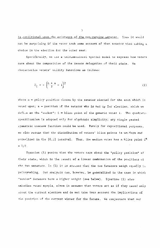
Specifically, we use a unidimensional spatial model to express how voters

care about the composition of the Senate delegation of their state. We

characterize voters' utility functions as follows:

—[n+a

— (1)

where n — policy position chosen by the senator elected for the seat which is

voted upon; a — position of the senator who is not up for election, which we

define as the 'anchor"; i — bliss point of the generic voter i. The quadratic

specification is adopted only for algebraic simplicity; any single peaked

symmetric concave function could be used. Purely for expositional purposes,

we also assume that the distribution of voters' bliss points is uniform and

normalized in the [0,1) interval. Thus, the median voter has a bliss point j°

- 1/2.

Equation (1) posits that the voters care about the "policy position" of

their state, which is the result of a linear combination of the positions of

the two senators. In (I) it is assumed that the two Senators weigh equally in

policymaking. Our analysis can, however, be generalized to the case in which

"senior" Senators have a higher weight (see below). Equation (1) also

embodies voter myopia, since it assumes that voters act as if they cared only

about the current election and do not take into account the implications of

the position of the current winner for the future. We conjecture that our

qualitative oonolusiona would not be altered by the explioit oonsidaration of

voters' foresight. Even though the voters would be less prone to support an

extreme oanddate solely for the immediate benefit of belanoing an extreme

anchor, substantial balaooing should still ooour, pertioularly if the future

is discounted. We also do not model how state level balancing in senate

eleotions interaot with balanoing at the national level (see Fiorina 1988,

Alesine and Rosenthal 1989a,b), although we oontrol for these effeots in our

empirioal work below.

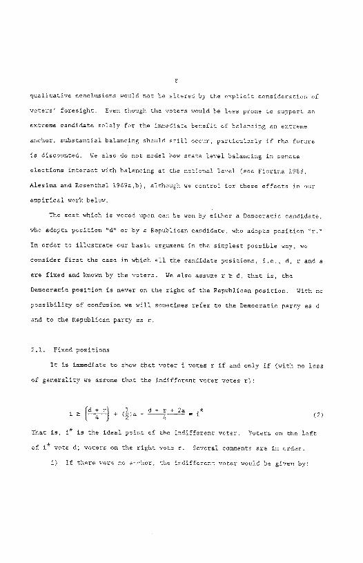
The seat whioh is voted upon oan be won by either a Demooratio oandidata,

who adopts position "d" or by a Republican candidate, who adopts position

In order rc illustrate our basic argument in the simplest possible way, we

consider first the case in which all the candidate positions, i.e., d, r and a

are fixed and known by the voters. We also assume r d, that is, the

Democratic position is never on the right of the Republican position. With no

possibility of confusion we will sometimes refer to the Democratic party as d

and to the Republican party as r.

2.1. Fixed positions

It is immediate to show that voter i votes r if and only if (with no loss

of generality we assume that the indifferent voter votes r):

(d+r) ,]L d+r+2a *i. R + ç)a i (2)

That is, i is the ideal point of the indrferent voter. Joters on the left

of i vote d; voters on the right vote r. Several comments are in order.

i) If there were no anchor, the indifferent voter would be given by:

9

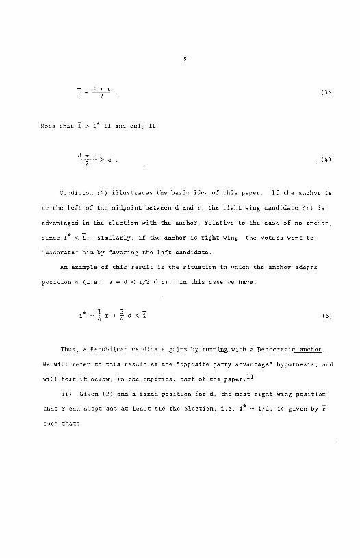
1-. (3)

Note that > if and only if

(4)

Condition (4) illustrates the basic idea of this paper. If the anchor s

to the left of the midpoint between d and r, the right wing candidate (r) is

advantaged in the election with the anchor, relative to the case of no anchor,

since i < i. Similarly, if the anchor is right wing, the voters want to

"moderate him by favoring the left candidate.

An example of this result is the situation in which the anchor adopts

position d (ie. , a — d < 1/2 < r). In this case we have:

i*_r+d<I (3)

Thus, a P.epubljcan candidate gains by running with a Democratic anchor.

Ce will refer to this result as the opposite party advantage" hypothesis, and

will test it below, in the empirical part of the paper.11

ii) Civen (2) and a fixed position for d, the moat right wing position

that r can adopt and at least tie the election, i.e. i — 1/2, is given by

such that:

10

r 2 — d — 2a (4)

Thus, the more left wing is a, the mote tight wing r ten he and at least

tie the election. This is due to the fact that the mote left wing is the

anchot, the mote moderation on the tight is desited by the votets. This

result mey hint at a polarization trend" in a dynamic eetting. If t becomes

more extreme, in the next election he will be the anchor, enabling the d

oanddete to be extreme and still win. If an extreme d becomes the anchor,

then r can be mote extreme in the next round, end so on. Since we have not

developed a dynamic model, it is impossible to explicitly characterize this

adjustment through time; however, condition (6) suggests a possible basis of

increasing polarization.

Figure 3 illustrates out argtosents. In Figure (3a) we represent a

standard teo—candidate contest with no anchor. The policy space is the

intenal [0,11, the median voter is at 1/2, d — 1/3 and r 2/3. In this case

-. d+t 1 ..the rnatfoetent voter is —y— — . The election is a tie. In rigute

(3b) we consider an election with the same positions for d and t, but with a

left wing anchor; that is, a d — I/I. In this case the indifferent voter

is i 5/12 ms implied by (5). Thus voters with ideal points between 5/12

and 1/2 vote d in the election without the anchor, but vote r in the election

with the anchor; in the second case, candidate r wins the election. Figure

(3°) illustrates that given a — d — 1/3,the moat tight wing position that m

can take and still tie is given by r — 1. Thus, for these parameter values r

can be as tight wing as the moat extreme position in the policy space and

still at least tie. Remember that without the left wing anchor, r would lose

the election if he chooses a position to the tight of 2/3 (Figure 3a).

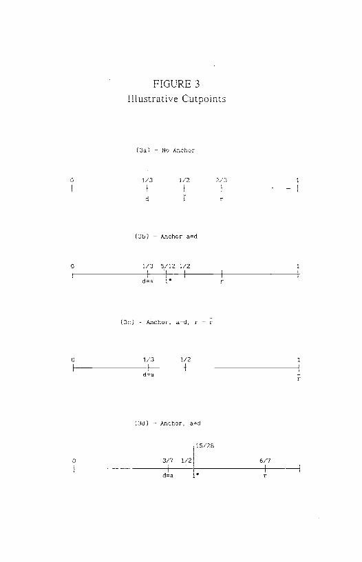
FIGURE 3

Illustrative Cutpoiuts

0

(3b) — Anchor ad

1/3 5/12 1/2 1

d=a 1 F

(3c) — Anchor, ad, r = r

0 1/3 1/2 1

Id=a —

F

(3d) - Anchor, a=d

?

115/28

:: 1/26

0

F

(3a) — No Anchor

1/3 1/2

d I

2/3

F-l

11

Finally, it should be noted that out framework is not inoonsistent with

the oase in which two Senators of the same patty ate elected. This

possibility is illusttated in Figure 3d. Suppose that a d 3/7 and

6/7. In this case i* 15/28 and d wins the eleorion. Clearly, two

Senatots of the same patty ate eletted when theit position is much oloser to

the median than that of the opponent. 12

Out results can be generalized to the tase in which the anchot and the

new Senator weigh differently in polity fotmulation. Suppose, again that the

anthor is 1eft wing (i.e., to the left of the median votet and to

the left of and mote influential in polity fotmulation than the new

Senator. Then, the t tandidate reoeives mote votes (fot given d, t and a) the

higher is the weight of the anchor in policymaking. In addition, for given d

and a the higher is the weight of the anchor, the mote right wing r oan be and

still win.

Differential weight in polity can be explained by multiple

considerations. Seniority is one: a more senior senator is likely to be mote

influential in policymaking than a freshman. Thus, if the anchor, who has

been in office for some time, is senior to the new Senator, he may be more

influential. Another consideration is "mandate." Ceteris paribus, an anohor

who had been elected with a landslide is likely to be more influential than if

he had barely won his seat in a highly contested race. In general, the

"opposite party advantage" end the "polarirarion trend" are stronger the lower

the weghr of the new senator. This is because more voters will turn to an

"extreme'S left (right) wing candidate in order to moderate a very powerful

right (left) wing anohor.3

12

3. Mobile Candidates

We now consider models in which the candidates can choose their

positions. We assume that candidates d and r have different preferences

(Wittman, 1977 1990; Calvert, 1935). The policy platforms chosen before an

election are "credible" in the sense that post—election policies cannot be

different from the pta—electoral platforms. (For a discussion of this

assumption see Alesina, 1938). There is uncertainty about the preferences of

the electorate,14 which can be captured by assuming that the extremes of the

uniform distribution of the voters' ideal policy are (w, i+w] where w is a

random variable with an expected value of zero, i.e., E(w) — 0, and a

cumulative distribution F(w)1

For given d, r and a, the probability that d wins the election is given

by:

P — prob[d wins] — prob{[i*—

w]> l/2}

I *— Prob[w < i — 1/2

- F{ + (1/2)a -1/2)

- (7)

Note that F is increasing in a and r; in particular, the more right wing

is the anchor the better the chances of the d candidate. The result

generalizes the "opposite party advantage" hypothesis, since it implies that

the probability that the d candidate wins is higher if the anchor is r than if

she is th Also note that,

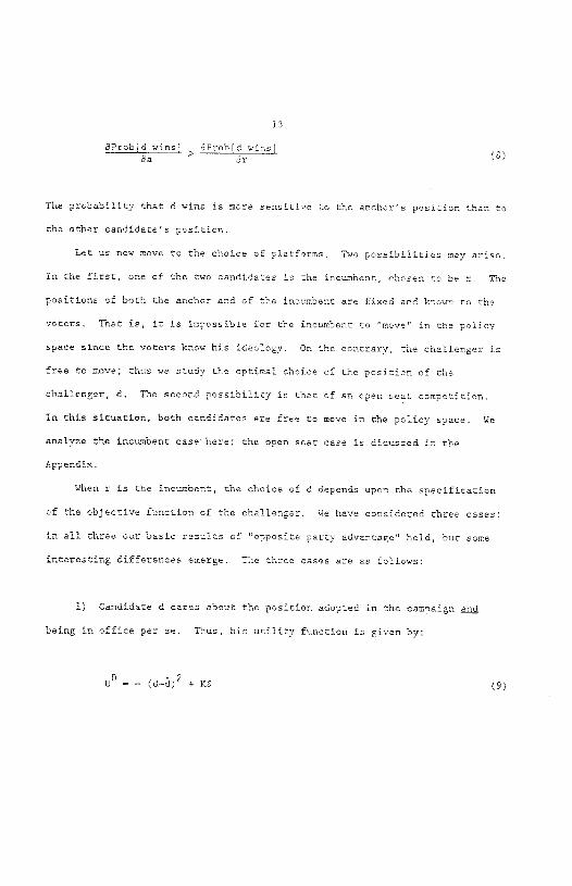
8Projins' j9bdwins(8)Ba Br

't'ne probability that d wins is more sensitive to the anchors position then to

the other candidates position.

Let us now move to the choice of platforms. TWO possibilities may arise.

In the first, one of the two candidates is the incumbent chosen to be r. The

positions of both the anchor end of the incumbent are fixed and known to the

voters. That is, it is impossible for the incumbent to "move" in the policy

space since the voters know his ideology, to the contrary, the challenger is

free to move; thns we study the optimal choice of the position of the

challenger? d. The maccod possibility is that of an open seat competition.

In this situation, both oandidates are free to move in the policy space. We

analyre the incumbent case here; the open seat case is dicussed in the

Appendix.

When r is the incumbent, the choice of d depends upon the specification

of the objective function of the challenger. We have considered three cases:

in all three cur basic results of "cppcsite party advantage" hold, but some

interesting differences emerge. The three cases are as follows:

1) Candidate d cares about the position adopted in the campaign

being in office par se. Thus, his utility function is given by:

(dd)° + KS (9)

14

where C is the party bliss point; K > 0 is the utility of being in office and

& — 1 if and only if d is elected, and zero otherwise,

2) Candidate d cares about the position he adopts only if he wins; thus,

his utility function is:

— [-(d—d)2 + (10)

3) The candidate cares (as the voters) about the policy outcome and

about winning pet se. Thus, the challenger's objective function is given by:

C0 — — ( — 0)2 + KS (11)

Case

The problem faced by party d is the following:

Max —(d — d)2 + P(d,r,a)K (12)d

In (12), P() is the probability that d wins, given in (7).

The first order condition is:

K - 2(d-d) (13)

The left hand side represents the marginal benefit of convergence, since it is

15

composed of the marginal gain in probability (remember that > 0 if

d C r) of a move to the right multiplfed by the utility of being in office.

The tight hand scue epresents the marginal cost of deviating from party d's

ideal policy d. The maximum is obtained at the point in which marginal costs

equal margfnel benefits.16

Several comments are in order:

i) In equilibrium a < d a r. If d � d the right hand side of (13) is rero or

negative and the left hand side is positive. If d > r > a the right hand side

is posirve and the left hand side negative.

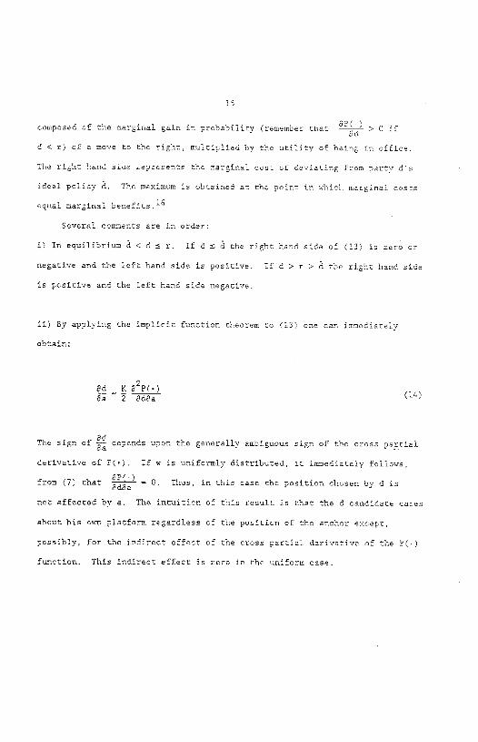
ii) gy applying the implicit function theorem to (13) one can immediately

obtain:

3d K 32p(.)(14)3a 2 BdSa

The sign of depends upon the generally ambiguous sign of the cross partial

derivative of P(S). Tf w is uniformly distributed, it immediately follows,

82() . . . . .from (7) that 0. Thus, in th:s case the position cnosen by d is

not affected by a. The intuition of this result is that the d candidate cares

about his own platform regardless of the position of the anchor except,

possibly, for the indirect effect of the cross partial derivative of the P()

function. This indirect effect is rero in the uniform case.

16

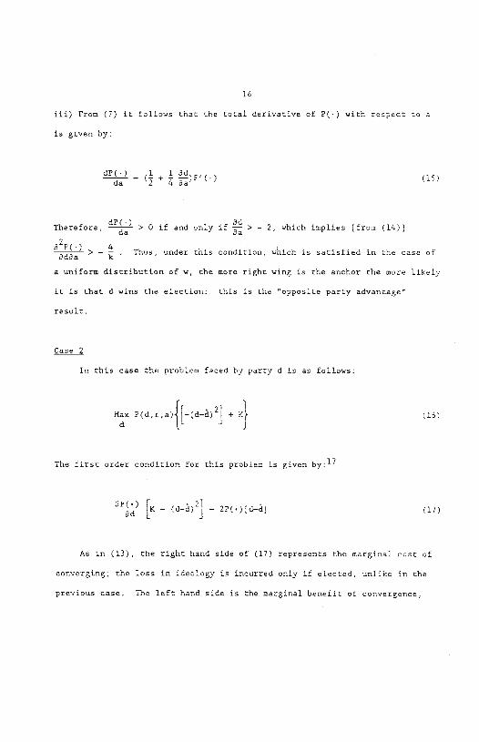
iii) From (7) it follows that the total derivative of P() with respect to a

is given by:

dP() 1 1 3d— ( + —)F (.) (it)

Therefore, > 0 if and only if > — 2, which implies [from (14))

32p!) 4> — — Thus, under this condition, which is satisfied in the case ofcd3a k

a uniform distribution of w, the more right wing is the anchor the more likely

it is that d %lins the election: this is the "opposite party advantage"

result

Case 2

In this case the problem faced by party d is as follows:

Ma P(dra){[_(d_d)2] +K}

(16)

The first order condition for this problem is given by:17

[K — (d_a)2]— 2P(.)[d-d[ (17)

As in (13), the right hand side of (17) represents the marginal cost of

converging; the loss in ideology is incurred only if elected, unlike in the

previous case. The left hand side is the marginal benefit of convergence,

17

which is positive, since the term [K—(da)°] represents the total value of

being in office. Note that this term has to be positive in equilibtium;

othese the utility level fot patty d would be higher when out of office

then when in office. In other words the loss entailed by a candidate taking

a position other then his ideal point must not exceed the value of the office

As in case 1, n equilibrium we have A C d S r. (The second inequality is

strict for K sufficenrly low.) Under mild suffcienr conditions, discussed

in the Appendix, whith imply that the cross partial derivative of P(") is not

3dtoo large, one can show that v- C 0. That is, tne more right wing :s the

anchor, the more left wing is the position chosen by candidate d. As

emphasized above, the sufficient condition on the cross partial derivatives of

P() is satisfied in the case of the uniform disrriburion of w as well as by

more general distributions (see Appendix).

This last result hints at the possibility of the dynamic "polarization

trend" discussed above in the context of the fixed position model. Note that

this trend would be bounded by the ideal points of the two candidates. That

is, in equilibrium the positions of d and r would always be in the interior of

the interaal bounded by d and . T'nus, the "polarization trend" would nor be

explosive.

Finally, under mild sufficient conditions on the cross partial

derivatives of P() which are discussed in Appendix and are satisfied in the

uniform case, the "opposite parry advantage" holds in this case as well.

Namely we have:

÷ > 0 (18)da Ba 3d Ba

18

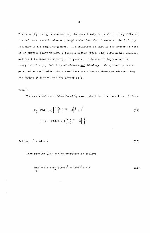
The more right wing is the anchor, the more likely it is that, in equilibriwn,

the left candidate is elected, despite the fact that d moves to the left, in

response to a's right wing move. The intuition is that if the anchor is more

of an extreme right winger, d faces a better "trade—off" between his ideology

and his likelihood of victory. In general, d chooses to improve on both

"margins"; i.e., probability of victory g ideology. Thus, the "opposite

party advantage" holds: the d candidate has a better chance of victory when

the anchor is r than when the anchor is d.

Case 3

The maximization problem faced by candidate d in this case is as follows:

Max (d,r.a){[._{__ — + K] (19)

+ [1 —P(d.ra)){ - }2}

Define: d — 2d — a (20)

Then problem (19) can be rewritten as follows:

Max P(d,r,a)( [(r—d)2 — (d-d)21 + K} (21)

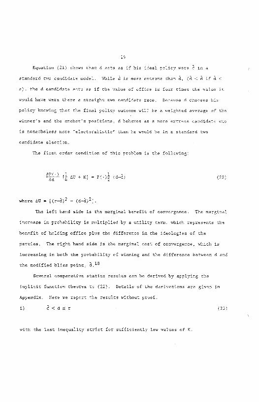
Equation (21) shows that d acts as if his ideal policy were d in a

standard two candidate model. Thile I is more extreme than I, (d C I if I C

a) the d candidate acts as if the value of office is four times the value it

would have were there a straight two candidate race. Because d chooses his

policy knowing that the final policy outcome will be a weighted average of the

winner's and the anchor's positions d behaves as a more extreme candidate who

is nonetheless more Thlectoralistic" than he would be in a standard two

candidate election.

The first order condition of this problem is the following:

U + El P(•) (d—d) (22)

where dU [(r—a)2 — (d—d)2J.

The left hand side is the marginal benefit of convergence. The marginal

increase in probability is multiplied by a utility term, which represents the

benefit of holding office plus the difference in the ideologies of the

parties. The mghr hand side is the marginal cost of convergence, which is

increasing in both the probability of winning and the difference between d and

the modified bliss point,

Several comparative statics results can be derived by applying the

implicit function theorem to (22). Derails of the derivations are given in

Appendix. Here we report the results without proof.

i) I<d�r (23)

wrh the last inequality strict for sufficiently low values of K.

23

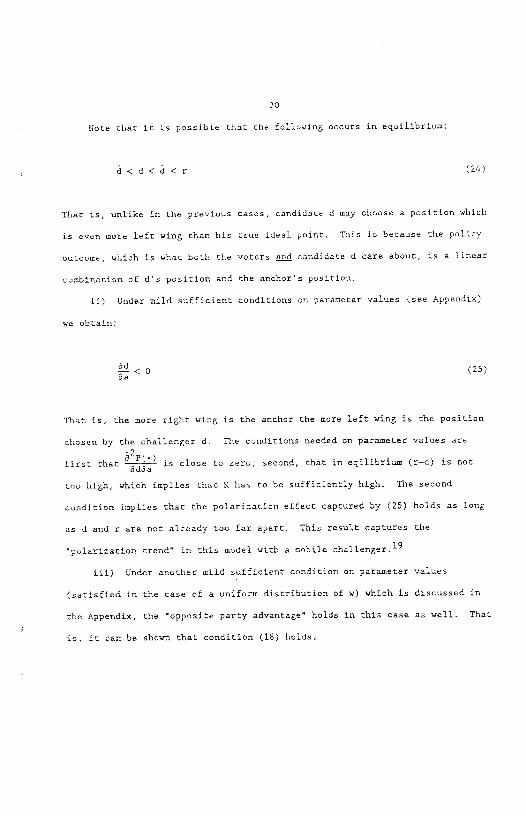
Note that it is possible that the following occurs in equilibrium:

d<d<d<r (24)

That is, unlike in the previous cases, candidate d may choose a position which

is even more left wing than his true ideal point. This is because the policy

outcome, which is what both the voters and candidate d care about, is a linear

combination of d's position and the anchor's position.

ii) Under mild sufficient conditions on parameter values (see Appendix)

we obtain:

(25)

That is, the more right wing is the anchor the more left wing is the position

chosen by the challenger cL The conditions needed on parameter values are

first that is close to rero; second, that in eqilibrium (r—d) is not

too high, which implies thac K has to be sufficiently high. The second

condition implies that the polariration effect captured by (25) holds as long

as d and r are not already too far apart. This result captures the

"polarization trend" in this model with a mobile challenger.19

iii) Under another mild sufficient condition on parameter values

(satisfied in the case of a uniform distribution of w) which is discussed in

the Appendix, the "opposite party advantage" holds in this case as well. That

is, it can be shown that condition (18) holds.

21

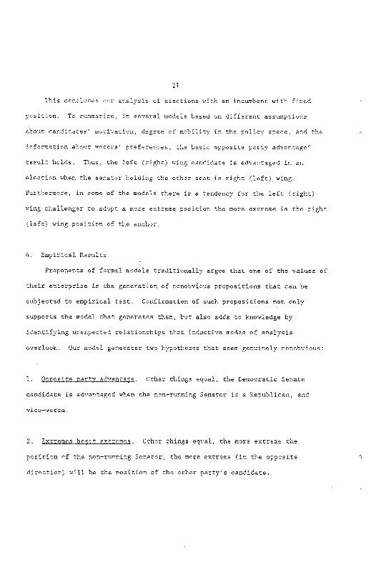
This concludes our analysis of elections with en incumbent with fixed

position. To summatire in sevetal models based on diffetent assumptions

about candidates' motivation, degtee of mobility in the policy space and the

infotmetion about votets' prefetences, the basic opposite petty advantage"

result holds, Thus, the left (tight) wing candidate is advantaged in an

election when the senatot holding the othet seat is right (left) wing.

Futthermore, in some of the models thete is a tendency fot the left (tight)

wing challenger to adopt a mote extreme position the mote extreme is the tight

(left) wing position of the anchot.

4. Empitioal Results

Proponents of fotmal models traditionelly argue that one of the values of

their enterprise is the generation of nonobvious propositions that can be

subjected to empirical test. Confirmation of such propositions not only

supports the model that generates them, but also adds to knowledge by

identifying unexpected relationships that inductive modes of analysis

overlook. Our model generates two hypotheses that seem genuinely nonobvious:

I. Other things equal, rhe Oemocratic Senate

candidate is advantaged when the non—running Senator is a Republican, and

vice—versa.

2. ypgpecpgg,r extremes. Other things equal, the more extreme the

position of the non—running Senator the more extreme (in the opposite

direction) will be rhe position of the other party's candidate.

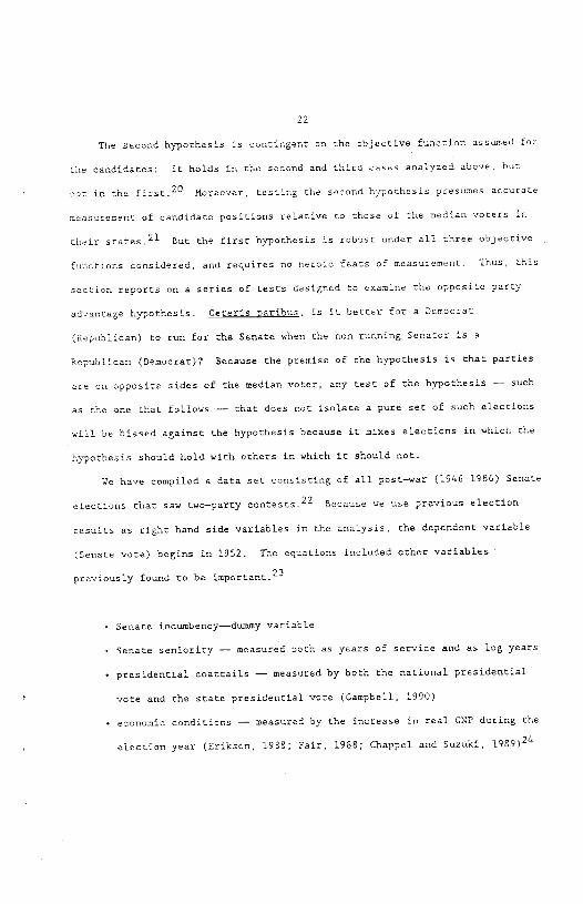
22

The second hypothesis is contingent on the objective function assumed fot

the csndidstes: it holds in the second snd third cases enelyted above, but

not in the first.2° Moreover, testing the second hypothesis presumes accutate

rzeasucement of csndidate positions relative to those of the median votets in

their states.21 But the first hypothesis is robost under all three objective

iunctions considered, and requires no heroic fests of measurement. Thus, this

secticn reports on e series of tests designed to examine the opposite perry

advantage hypothesis. Cererie peribus, is it better for a Democrat

(Republican) to run for the Senate when the non—running Senator is e

Republican (Democrat)? Because the premise of the hypothesis is that parties

are on opposite sides of the median voter, sny test of the hypothesis — such

as the one that follows — that does not solare a pure set of such elections

will be biased against the hyporhess because it mixes elections in which the

hypothesis should hold with others in which it should not,

We have compiled a date set consisting of all post—war (1946—19%) Senate

elections that saw two—party contests.22 Because we use previous election

results as right hand side variables in the analysis, the dependent variable

(Senate vote) begins in 1952. The equations included other variables

previously found to be important.23

• Senate incumbency—dummy variable

• Senate seniority — measured both as years of service end as log years

• presidential coattails — measured by both the national presidential

vote end the state presidential vote (Campbell, 1990)

• economic conditions — measured by the increase in real GM? during the

election year (Erikson, 1988; Fair, 1988; Chappel and Sumuki, 1989)24

23

previous vote — lagged vote for the Senate seat in question (normally

six years previously, but oocasfonally more retent if a speoial

election were held)

time trend — introduced to account for any secular national

improvement in Republican senatorial fortunes

midterm effect — duessy variable for control of the Presidency

[Erikson, lPfS; Alesina and Rosenthal (lSBSa,b)[.

We fully expected these variables to attount for the lion's share of the

variance in Senate elections over time. As it turned out, economic

conditions, fncumbency, lagged vote, and the midterm effect were important.Zt

The most interesttng question is whether the non—running Senator has any

effect over and above these variables.

Note that the correct econometric specification for representing the

anchor seat effect when testing the opposite party advantage hypothesis is not

a dummy variable for the party of the anchor, aa intuition might suggest. Let

us return to our simplest model, with fixed party positions and no

uncertainty. Assume that in every state, j, voters are uniformly distributed

on [0,1] and that the parties take positions d. r,j. (T'nere is no loss of

generality here other than uniformity, since the origin and length of the

space of some underlying national liberal—conservative continuum could vary

across states without changing our results.) Assume that the party positions

are sufficiently close to symmetric about the median (1/2) that all states

have split delegations. The inequalities that define this situation arem < 2—3d, and d, > 2—3r, . T'ne algebra of the model indicates thatJ J

24

— lOO(2rd4) —Vra.j

where Vi is the Republican vote percent, and is the Republican vote

percent in the preceding election for the anchor.

Thus, each state would have a different intercept, and the coefficient on the

anchor vote would be —1. In light of this argument it would not be correct to

estirate an equation of the form:

+B11j

where I is a dummy variable for the party of the anchor seat, and

I — 1, 2 are coefficients.

In summary, then, the anchor vote is a proxy variable for the positions

of the two parties. Indirectly, the plurality of the anchor influences the

share of votes received by senators competing for the other seat.

Of course, there might be other States where party positions were such

that one party always wins both seats. This could happen, for example, if

both parties were to the same side of the median. For these states we would

have

Vrj —

In these states, regressing on either the anchor vote or an anchor dummy

variable would be inappropriate. If our actual sample includes a mixture of

25

split delegations and unified delegation states and we regressed on the anchor

vote, our estimated regression coefficient would be less than 1.0, since it

would be an average of the 1.0 from the split states, and the 0,0 from the

unified states,

In real elections the relationship between the anchor position, the

anchor vote and the current vote will be more complex than that generated by

our simple model with a uniform distribution of preferences. It will depend

on factors fncluding (a) the distribution of voter preferences, (b) changes in

voter preferences between elections, (t) the objectives of the candidates,

(d) the relative weights of the anchot and contested seats. Consequently, the

functional form of the relationship in general can not be specified. We can

only ask whether past and current votes have a statistical relationship. As

is commonly the case in empirical work, a linear term worked best;

transformations, dummies, and interactions added little. Therefore, the

results we report are based on equations in which the anchor vote affects the

current vote in simple additive fashion.26

The first column of Table I contains a simple regression that accounts

for about half the variance in postwam Senate elections, Tne estimates

suggest that

1. Running as an incumbent is worth about four points.

2. Running in a mdterm election costs candidates of the president's

patty between 2 and 3 points. Thus, in the current period of

Republican presidential dominance, Republican senatorial candidates

are disadvantaged.

26

3. Every one point increase in ONE growth during the election yeat is

worth ebout half a point for candidates of the presidential party -

4. There is a very small but significant Rapublican trend in post wet

Senate races.

5. There is quite a bit of slippage from one election to the next, as

the coefficient on the vote six years earlier is only about .25

6. The vote garnered by the non—running Senator two or four years

earlier is negatively related to the vote in the next election?

although the estimate is not significant.

The first four results are straightforward and in keeping with previous

findings in the literacure. The fifth finding is mildly surprising but quite

in keeping with the image of Senate elentions as volatile and idiosynnratic.

The sixth finding is most intriguing: the opposite patty advantage hypothesis

meets with some weak support. With this bit of encouragement we pushed on.

In the second column of Table I the effents of the two previoum elections

have been estimated aeparately for elentions contested by incumbents and those

in which the Senate seat is open.27 Now an interesting disparity appears. In

incumbent—contested seats the vote in the election two years or four years

earlier bears a significant negative relationship rn the current vote (t—l.7.p C .05, one—tailed test). Roughly, there is a 7 pnrnenr "tax" or penalty on

the parry'a previous vote margin. In open seat rarrs, no such penalty

appears. Instead, both the lagged vote and snchnr vote have similar positivecoefficienca.

In the third column of the table we take she next Ingical step, that of

dividing the effecra of previous elections arnsrciing to whether the election

27

occurs 5.n a presidential or off—year This estimarion reveals rhat the

negative relatiooship between the votes in adjaceot Senate elections is

strongest in presidential election years with incumbents ruooiog2 Roughly

speaking, in such elections for every vote a partys candidate got in the

previous Senate election, the party's current candidate loses one fifth of a

vote, a penalty of nearly 20 percent. No negative relationship emerges in

mid—term years or in presidential years without incumbents running.29 A

reexamination of the model suggests a possible explanation for the

presidential year finding. Middle—of—the—road voters, those whose ideal

policy lies between those of the two parties, are those most lilcoly to engage

in "balancing" behavior (Figure 3). If presidential electorates contain more

such moderate voters than the smaller mid—term electorates, thon we would see

more evidence of balanong behavior in the former.

We wish to emphasime the importance of the results in Table 1. in any

pair of temporally adjacent elettions, zz ).e1s.ofwhg.thg.nintumbeni.s are

senmelettion, researchers would expect to find a strong positive

relationship between a party's vote in one election and its vote in the next,

and one would expect the relationship to deteriorate as the elections become

more separated in time. To underscore this point consider the reletionship

between current election results end previous results in Mouse elections. In

Table 2 the Republican vote in 1976—fl—SO House elections is regressed on the

Republican vote one election and two elections earlier,30 As one would

expect, the returns in both earlier elections are positively related to those

in the current election, but those from the closer election have a much

stronger relationship than those from the more distant election. Although

this pattern is stronger for inoumbents, it is clearly true for open seats as

28

well, except fct the anomolous insignificant negative coefficient fot the 1978

mid—term (based on only 34 observations). Thus, a House candidate's vote

bears a significaLs positive relationship to the vote for the (different)

candidate of his party in the previous election. In contrast, as Tahle I

shows, a Senate incumbent's vote has a significant negative relationship to

the vote for his party's (different) candidate in the previous election, at

least in presidential election years. This is a herecofore unnoticed

empirical disparity.

In order to highlight even more clearly the surprising difference in the

lag structure of House and Senate elections, we have run for the Senate the

same regressions reported ic Table 2 for the House. The coefficient on the

first lag effectively zero, reversing the normal relationship fo aggregate

election returna (Table 3).

Finally, we heve also rested whether voters seek to balanue with their

vote the overall composition of the Senare, rather than their state

delegation. To control for this different type of balancing we defined a

variable, Republican sear share in the Senere preceding the election under

consideration. This variable was added to our regression but was never

significant: the t—atariatic on irs coefficient never reached the value of I.

A theoretical account conaisrenc with this finding runs as follows. Voters

care both about national policy ourcoc.es and about how the Senators of their

state articulate the state positions The focus of this paper, balancing or

the state level, is relevant for the definition of the state position.

National policy outcomes, in contrast, are affected by the interaction between

the House, the Senate and the President. Ar the national level, the releveur

balancing involves an executive—legislative Interaction which is captured by

29

the aid—term variable in our regression. That is, the voters are not

interested in a balanced Senate per se, but in a balanced executive—

legislative package

5. Conclusion

This paper has developed a general nodal based on the noricn that voters

n Senate elections take account ci the existence of the non—running Senator

when deciding how to case their votes. Under several different assumptions

regardingthe candidate objective functions, the model predicts an "opposite

party advantage:" Republican Senate candidates are somewhat advantaged when

the non—running Senator is a Democrat, and vice—veras. This result is

generally stronger the greater the influence of the non—running Senator

relative to that of the one who will be chosen in the currant election.

Somewhat less robust but still rather pervasive is an "extrcmes permit

extremeC result: the more extreme the position of the non—running Senator,

the more extreme can be the position of the candidate of the oppusing party.

The reason i5 that the basic logic of the model is one of balancing. Ii an

ideologue somehow wins election, moderate voters can only counter—balance her

positions by choosing an opposite ideologue. It seems possible that in a

dynamic extension of our models, the extremes permit extremes feature could

give rise to a polarization process that would see a state's Senate candidates

grow increasingly distant over time. We grant that the models discussed make

heavier informational demands on voters than most political scientists would

find plausible. But the voters need not know the specifics of the candidates'

stands; rather, they need only have an impression of the position of the

candidates relative to each other and to the non—running Senator. At any

30

rate, the empirical analysis produces results of a qualified positive nature.

Ar leaat in presidential elections, incumbents of one parry suffer a vote

penalty if the non—running Senatot is of the sese party. Given that half of

all Senate elections occur in presidential years, and about three—quarters ef

incumbents seek re—election, about 40 percent of conresporary Senate elections

fall into this category. Whatever the desands our model makes on voters, it

is the only one of whIch we are aware char can account for this new finding.

Finally, we emphasize that although balancing behavior adds en

interesting twist to parry fortunes in Senate elections, it is certainly nor

the major determinant. It is still better to be an incumbent, to have a

healthy economy (if your parry's president is in office, a poor economy

otherwise), and to have a strong parry base in your stare. Moreover, our

equations explain just a bit more than half the variance in post—war Senate

elections, consistent with exisring characterizations that emphasize their

volatility and unpredicceblliry. Despite their noisy quality end the larger

forces that are at work in Senate elections, however, at the margins small

movements of votes can derermine who wins end who loses. Salancing behavior

may well underlie such movements.

Fcc too tes

1. The University of Nebraske sponsored a conference on the study of the

Senate in October 1988, and Rice University and the University of Nooston co-

sponsored e conference on Senate elections in November 1990. In additioo, the

American Nationsl Election Studies (ANES) has recently comploted the seoood

wave of a projected three—weve study.

2, In the five elections of the 1980s, 95 percent of all Noose iooorobents who

sought re—election were successful; the comparable figure for the Senate was

80 percent.

3. Election surveys show that many more voters can place the Senate

csndid.ates on seven—point scales than can place the Nouse candidates. And in

1980 the negative campaigns of conservative groups and RAGS were viewed by

many as the key to che Republican upsets. On the other hand, the Senate

electoral landscape abounds with examples of Senators attackod for boing cot

of touch with their states because of their national activities.

4. In the 1988 Senate elections, 78% of all votes cast weto consistoot wfth

the party identification of the voter, about the same as the figure for Nonse

elections (79%).

5. The answer is not the easy one — the rise of two—patty competition in the

South. chile there is a rise in split representation in the Southern states,

it accounts for less than half the trend identified in Ffgure 1.

6. Figure 2 was computed from the first dimension of the D—NONINATE scaling

with linear trend in legislator positions. For detaila on the scaling

procedure, see Poole end Rosenthal (1991;. Ubile the distanoe between

32

Senators of different parties is declining over rime, the distance between

Senators of the same party is also declining over time. In fact, the ratio of

the first curve (Senators ef different patties) and the avetage of the latter

two (Senators of the same patty) shows an incteasing ttend. At any tate, what

is most relevent for out model is the dispersion of Senators' position

relative to the distribution of voters' preferences; thete is no reason why

the latter should be constant over time. Thus, one csnnot say for certain how

changes in the distance between the Senators compete to changes in the

distribution of voters' preferences.

7. There is evidence, although it is disputed (for a survey see Brady, Btody

and Fetejohn, (1989) that Senators move toward the center as their election

draws near. Even if true, that does nor alter the fact that they remain

relatively distant from each other.

8. Using the new available 1988 Ametican National Election Studies Senate

data, Erikson (1989) shows that the distributions of Deooctat and Republican

Senate candidates (as viewed by the relevant state electorates) do not

overlsp. That is, the most conservative Southern Deacctat is seen as to the

left of the most liberal Eastern Republican.

9. with one exception: The identical insight has been explofted by Michael

Krassa (1989). The idea is a natural extension of the aodels of President—

House voting developed in Fiorina (1988) and Alesina and Rosenthal (1989a,b)

10, On rare occasions an incumbent dies or recites and the election to fill

the vacant meet occurs at the saae time as the regular election for the other

seat. By our count this has happened only 14 tiaes in tore than 725 Senate

contests since 1946, so we will ignore that possibility in what follows.

33

11. It should be noted that in our model balancing occurs within each state.

Thus, the opposite patty advantage refers to each state race viewed

separately, This, of course, sterns from our model of voter's preferences.

embodied in (1). More generally, voters may want to balance, with their vote,

the Senate as a whole. In this case, the "opposite party advantage" would ha

enjoyed by, say a Republican candidate running when the majority of the

Senate is Democratic, in the empirical part of the paper we will test (see

below) whether balancing occurs at the state level or at the level of the

Senate as a whole.

12. Two senators of the same party are always elected if both parties (ecd

the anchor) are on the same side of the median,

13. An additional case is one in which one of the two candidates is an

incumbent which is senior even to the anchor. Derails of this case are

available fram the authors.

14. Without this uncertainty the model would be trivial since for any

combination of polity positions the electoral result would be perfectly

predictable. in such a model, even ideological candidates would fully

converge [Calvert (1985)].

15. See Alesina and Rosenthal (l989a,b) for an identical formalimarion of

uncertainty about voters' preferences.

16 ______If S 0 holds, the second order condition of this problem is

satisfied. Henceforth, we assume that this sufficient condition i5 satisfied.

17. See note 14.

18. See note 14.

34

19. In a dyrtamic model this condition may suggest thrt there is a limit to

the "dynamic polarization trend."

20. Additionally, in the case where parties have fixed positions (because nf

reputational or other considerations), the hypothesis evidently would not

hold.

21, It is easy enough to scale the roll call votes of sitting Senators,

though not all critics would be convinced that problems of measurement

equivalence over time can be overcome. Unfortunately, ascribing positions to

defeated challengers and state electorates is mote difficult, though Wright

and Serkman (1986) point out that this Information is available for 1982 at

least.

22. Given the nature of the hypothesis being tested we naturally had to omit

the elections in which special Senate elections occurred at the same time as

the regular election. Additionally, we eliminated those races in which third

parties got more than 10 percent of the vote, and races in which the losing

candidate got less than 15 percent. Cumulatively, these decision left us with

a total of 458 obserzations, but only fifty from the stares of the old

Confederacy.

23. We estimated models that allowed each state to have a different intercept

(that is, "normal vote"). For such "fixed effects" models it is well known

that OLS provides consistent estimates of the other linear parameters but

inconsistent estimates of the error variance and the intercepts. Since our

interest is in the linear parameters for the independent variables, the

inconsistency problem is not a concern except insofar as the biased error

variance affects significance tests. Since the bias is on the order of l/T,

where T is the number of observations per state, the bias is not a serious

problem, given that we average 11 observations per srere. In standard

fixed—effeots models there would be an identjoal number of times—series

observations for eaoh state. As this is nor true in our oase (beoause of

omitted eleotions (see previous footnote) we wrote a GAUSS program (available

on request) that estimates the model for varying numbers •of observations.

24. We exsmined a number of measures of national eoonomio oonditjeus as well

as state real inoome figures generously provided by John Chubb. CUP growth

gives the strongest results.

25. Neither measure of the presidential vote (netional, state) was ever

signifioant when CUP was in the equations. Seniority did not improve the fit

of the equations beyond the simple dummy variable for inoumbenoy. We tan the

equations with and without a trend term; though signifioant, exoluding It has

no effeot on other ooeffitients.

26, There is another justification for a linear speoifioation. In the

generalized version of the model (appendix), the magnitude of the opposite

patty effett varies directly with the power" or influenoe of the anohot

Senator. If we take the latters electoral margins, or mandates, as one

element of their 'power," then the strength of the opposite patty advantage

should very directly with the wote margin of the anchor Senator. Thus, there

is substant!ve, as well as statistical justification for intluding the aotuai

magnitude of the anchor vote.

27. The suxary statistics indioste that we csn rejeot the hypothesis that

the coefficients are identical in the two types of eleotiens (p < .03). We

also estimated the effects of other variables seperately mt the two types of

elections but found no significant differences.

36

28. Given suggestions in the Gongressionsi litersture sbout important changes

in House elections during the mid—1960s, we also tried estimating separate

coefficients for pre—1966 and post—1966 races. No significant differences

emerged.

29. Note that the effects of previous elections for the some sest ste

pisusible. The relstionship is much stronger when incumbents run than when

they do not. The re1ationshp is again stronger in presidential years than in

off—years.

3G. Returns from the l9SGs did not pool with those from the 19]Gs, consistent

with the mid—1960s trsnsformation in House elections. We did not include

elections from the 196Gm because of the extensive redistricting that took

place in the middle of thst decade. The same 85% cut—off was used as in the

Senste analysis (footnote 19).

References

Alesina, Alberto, 1988. Credfbi1ity and Policy ' mcrgence in a Two—Perry

System with Rational Voters." American Economic Review, Vol. 78(4):796

806.

___________ and Nowatd Rosenthal. l989a. Partisan Cycles in Congresoionel

Elections and the Mactoeconomy, American Political Science Review

June Vol. 83:373—98.

__________ 1989b. "Moderating Elections." National Bureau of Rconomic

Research Working Paper No. 3072.

_________ John Lcndregan and Howard Rosenthal. (1990), "A Political

Economy Model of the United States." Unpublished.

Alford, John R. and John R. Nibbing. l989a, "The Disparate Electoral

Security of House and Senate Incumbents," Prepared for the 1989 American

Political Science Association Annual Meeting.

_________ 1989b. "Electoral Sensitivity in the United States Congreso.

Prepared for the 1989 Western Political Science Assccation Annual

Meeting.

Bernheim, Douglas, Bezael Peleg and Michael Whinsron. 1987. "Coalition Proof

Nash Equilibria. 1. Concepts." jpnaljE5QnomicTheo, June, Vol.

2:1—12,

Brady, David, Richard Brody and John Perejohn. 1989. "Constituency

Preferences and Senatorial Actions: Modeling the Representation of

Constituency Interests." Prepared for the Conference on Electing the

Senate, University of Houston end Rice University.

38

Calvert, Randall. 1985. "Robustness of the Multidimenaional Model, Candidate

Motivations, Uncertainty and Convergence." American Journal of Political

Science, June, Vol. 29:69—95.

Campbell, James E. and Joe A. Summers. 1990. Presidential Coattails in

Senate Elections. American PoJitical Science Review, Vol. 84:513—524,

June.

Downs, Anthony. 1957. An Economic Theory of Democracy. New York: Narpet

and Row.

Erikson, Robert. 1989. "The Puzzle of Midterm Loss," Journal of Politics,

Vol. 50:1012—1029.

__________ 1989. "Roll Calls, Reputations, and Representation in the US

Senate." Prepared for the Confetenoe on Electing the Senate, University

of Nouston and Rice University.

Petejohn, John A., Morris P. Piurina and Edward V. Paokel. 1980. "Non—

equilibrium Solutions fot Legislative Systems." Behavioral Boienoe, Vol.

25:140—148.

Piotina, Morris. 1988. "The Reagan Yeats: Turning to the Right or Croping

Toward the Middle." In B. Cooper, cC al., eds., ggsuggnoeof

Coneenatism in Anglo—American Democracies, Duke University Press:

Durham, MC, 430—459.

__________ 1974. Representatives, Roll Calls, and Constituencies

Lexington. MA: Lexington Books.

Cteenberg, Joseph. 1989. "Deriving Strong and Coalition Proof Nash

Equilibria from an Abstract System." Journal of Economic Theon,

Nuntington, S.N. 1977. "A Revised Theory of American Patty Politics."

American Political Science Review, Vol. 44:669—677.

Jacobson Gary. 1990. tElectoral0rinsofDi"tided0overmenc. Boulder,

CD: Wearview Press.

Kramer, 0,11. 1977. "A Dynamical Model Political Equil:oriur Journal of

Economic Theory, Vol. 16:310—334.

Krasaa, Michael A. 1989, "Compositional Voting and the Rational Preferonce

for Polarized Representation." Prepared for the Conference on Elocciug

the Senate, University of Houston and Rice University.

Poole, Keith T. and Howard Rosenthal, l964a. "U.S. Presidential Elections

1968—1980: A Spatial Analysis." American Journal of Political Science.

May, Vol. 28:282—312.

__________ 1984b. "The Polarization of American Politics." Journal of

Politics, Vol. 46:1061—1079.

___________ 1985a. "A Spatial Model fot Legislative Roll Call Analysis."

American Journal of Political Science, Vol. 29:357—84.

__________ 1991. "Patterns of Congressional Voting." Mglican Journal of

Political Science, forthcoming.

Shepsle, Kenneth A. and Barry R, Weingaat. 1984. "Uncovered Sets and

Sophisticated Voting Outcomes with implications for Agenda Institutions."

American Journal of Political Science Review, 28:49—74, February.

Wright, Gerald C., Jr. and Michael B. Berkman. 1986. "Candidates and Policy

in United States Senate Elections." American Political Science Review,

Vol. 80:567—590., June.

Wittsan, Donald. 1977. "Candidates with Policy Preferences: A Dynamic

Model." February, Vol. 14:180—189.

1983. "Candidate Motivation: A Synthesis of Alternatives."

American Political Science Review, Vol. 72:142—157.

41,

___________ 1990. "Spatial Strategies When Candidates Have Policy

Preferences. in Enelow, Jaaes and Melvin Hinich, eds. , Advances in the

Spatial Theory of Elections. Cambridge University Press, 66—98.

41

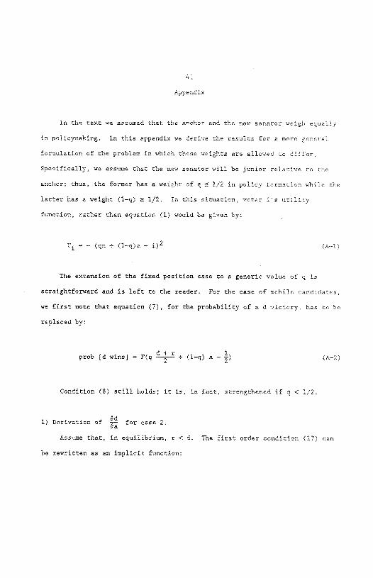
Appendix

In the text we assumed that the anchor and the new senator weigh equally

in policymaking. In this appendix we derive the results for a more general

formulation of the problem in which these weights are allowed to differ.

Specifically, we assume that the new senator will he junior relative to the

anchor; thus! the former has a weight of q � 1/2 in policy forrnaton while the

latter has a weight (l—q) � 1/2. In this situation, voter i's utility

function, rather than equation (1) would be given by:

(qn + (l-q)a — i)2 (A—I)

The extension of the fixed position case to a generic value of q is

straightforward and is left to the reader. For the case of mobile candidates,

we first note that equation (7), for the probability of a d victory, has to be

replaced by:

prob {d wins] — F(q 4— + (l—q) a — ) (A—2)

Condition (8) still holds; it is, in fact, strengthened if q < 1/2.

3d1) Dertvatron of — for case 2,

Sa

Assume that, in equilibrium, r < d. The first order condition (17) can

be rewritten as an implicit function:

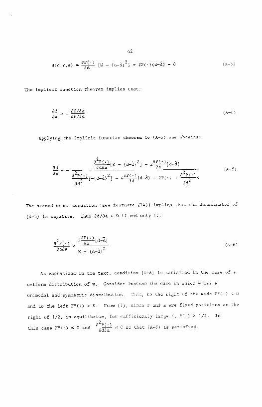
42

H(d,r,a) - [K — (d-d)2[ — 2P()(d-d) - 0 (A-3)

The implicit function theorem implies that:

— — (A—4)Ba BIT/3d

Applying the implicit function theorem to (A—I) one obtains:

3d 33[K - (d-d)2] - 2[d-d]— — — (A—s)Be

3H_(d_2— 4(d-d) - 2F() +

The second order condition (see footnote (14)) implies that the denominator of

(A—5) is negative. Ynus 3d/Ba < 0 if and only if:

2 2—1[d—d[3 P() ____________ (A—i)

BdBa K — (d—d)2

As emphasized in the text, condition (A—i) is satisfied n the case oi a

uniform distribution of w. Consider instead the case in which w has a

unimodal and symmetric distribution. Then, to the right of the mode F"() < 0

and to the left F"(') >0. From (7), since r and a are fixed positions on the

right of 1/2, in equilibrium, for sufficiently large K, f() x 1/2. In2

this case F"() s 0 and k_2_ � 0 so that (A—i) is satisfied.cd3a

43

2) Datvatjon of (18)

Using (4—2) it is immediate to show that:

- F'()(l-q) (4-7)

F'S (4—8)2

Using (A—7) and (A—f), it follows that:

¶11 F'[(l—q) (4—9)

Thus, dP/da > 0 if and only if:

> — (4—10)q

Finally, note that:

(4_il'Dd 21—q 8a

Substituting (A—f) into (A—l0), the lattet can be rearranged as follows:

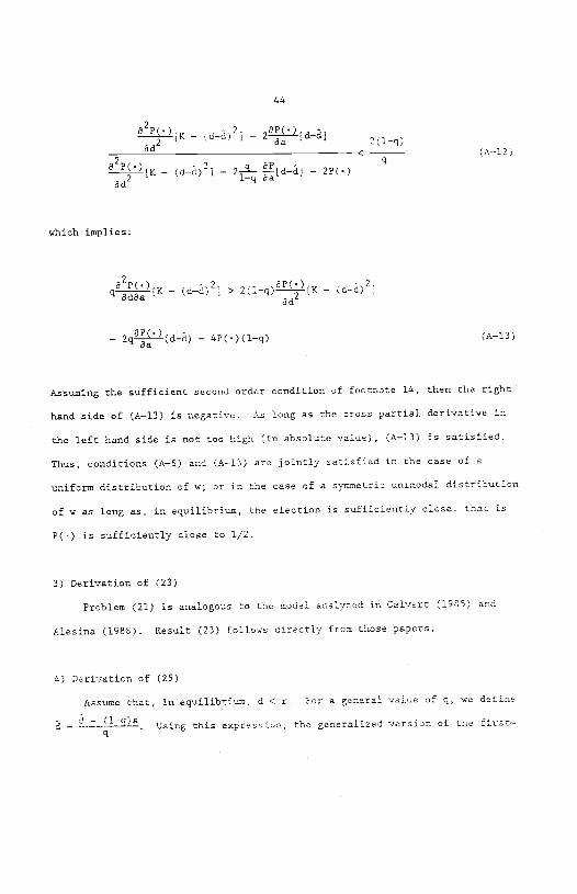
44

____ - (d-d)2] - 2fi[d-d) 2(l-q)C (A—l2)

____ - (d-d)2 - 2 F[d_al — 2P(.)q a

which implies:

q38[K - (d—ä)2) > 2(l-q)[K - (d-d)2}

—2q9i--t(d_-d)

— 4P(.)(l—q) (A—13)

Assuming the sufficient second order condition of footnote 14, then the right

hsnd side of (A—13) is negative. As long as the cross partial derivative in

the left hand side is not too high (in ahsolute value), (A—l3) is satisfied.

Thus, conditions (A—f) and (4—13) are jointly satisfied in the case of a

uniform distribution of w; or in the case of a symmetric unimodal distribution

of w as long as, in equilibrium, the election is sufficiently close, that is

P() is sufficiently close to 1/2.

3) Derivation of (23)

Problem (21) is analogous to the model analyzed in Calvert (1985) and

Alesina (1988). Result (23) follows directly from those papers.

4) Derivation of (25)

Assume that, in equilibrium, d C r. For a general valoe of q, we define

d — h.__3_1-_1?! Using this expression, the generalized version of the first—

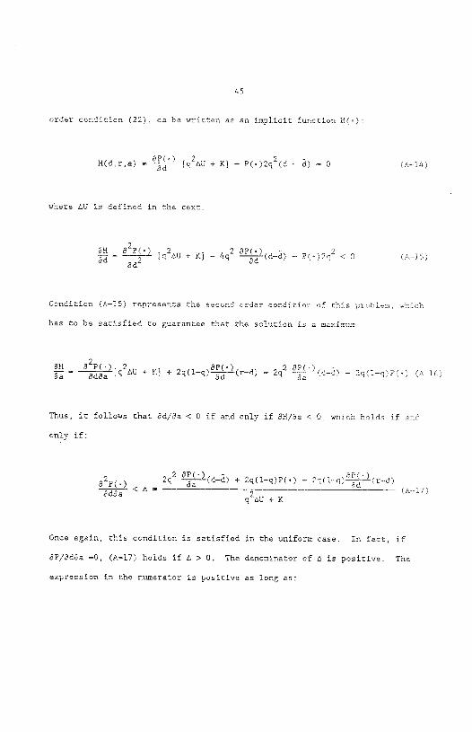
45

order oondiron (22) Os be written as an implicit function H():

H(d,r,a) ]q2LU + K] P(')2q2(d — d) 0 (Ai4)

where LU iS defined in the text.

H ]q2LU + K] 42 (d—d) P()2q2 < 0

Condition (A—if) represents the aeoond order condition of this prohie:s, which

hss to be satisfied to guarantee that the solution is a isaxiauss

32P(•)q2 + K] + 2q(l—q)(r—d) — 2q2 L'(d_d) — 2q(i_q)p(#) (It—SE)

Thus, it follows that fd/3a < 0 if and only if 3M/as < 0, which hoidc if and

only if:

2q ¶.1(d-a) + 2q(l-q)P(.) — 2q(1_q)2LL(r_d)(A-IS)a

qAU+K

Once again, this condition is satisfied in rhe uniform case. In fact, if

3P/3dôs O, (A—i7) holds if A > 0. The dencminaror of A is positive. The

expression in the numerator is positive as long as:

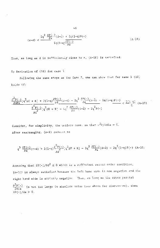
46

2q2 §ILJ(d_g) + 2q(l—q)P(.)(r—d) < 3P()

(A—IS)

Thus, as long as d is sufficiently close to r, (A—l8) is satisfied.

5) Derivation of (18) for case 3

Following the sane steps as for Case 2, one can show that for case 3 (18)

holds if:

32() 2 SP(') 2 aF() -

[q aU + K] + 2(l—q)----—--(r--d) — 2q —(d—d) — 2q(l—q)P()BdSa Sd < kCS.L (A—19)

SCfq2Au + K] — 4q2 (d—d) — 2q2P(')

Consider, for simplicity, the unifora case, so that 325/BdSa — 0.

After rearranging, (A—9) reduces to

q3 q(t-d) > 2(l-q)']q20U + K] — 2q3 (d-d) — 2q2(1-q)P() (A-20)

AssumIng that 8P()/3d2 � 0 which is a sufficient second order condItion,

(A—20) i5 always satisfied because the left band side is non negative and the

right hand side is strictly negative. Thus, as long as the cross partial

32P( )SdSa

is not too large In absolute value (see above for discussion), then

dP(')/da > 0.

47

6) Open seat competition

Consider the situation in whioh both candidate d and r are mobile since

neither of them is the inoumbenr. Oiven the reeults by Wirtman (1963) and

Calvert (1985), Cases 1 and 2 oan be easily analyzed. It is immediate to shcw

that in both oases, in equilibrium one obtains:

d<d�r<(0—21)

The compatative statios results discussed above iot these two cases

easily generalize. Some interesting issues arise in Case 3. For this case

the problem beoomes:

Max P(')](r-a)2 - (d-d)2 + K] (0-22)d

Max (I - P()](d—?)2 (r-)2 + K] (0-23)r

- — 1l—o)a.where r . Also we assume that the benefits oi botng tn oiitca (K)q

of being in offioe (K) is the same for both parties. We also need an

additional suffioient condition for the second order condition, i.e.,

82P(.)/8r2 > 0.

Problem (A—22) and (A—23) is identical to the model analyzed by Wittman

(1983) and Calvert (1985) i d and i are interpreted as the original ideal

points of the two candidates in a model without an anchor. Define a0 and i°

as the solution of that problem, i.e., of (A—22) and (0—23) inrerprctcd as a

Wittman/Calvert problem with nc anchor. Define d* and r the solution of (A—

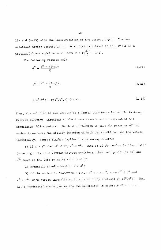
48

22) and (A—23) with the interpretation of the preaent paper. The two

aolutiona differ beoause in our model P(S) is defined in (7), while in a

Witrman/Calvert model we would have P F(h — 1/2).

The following results hold:

* ci° — (1— )ad (A—24)q

— (l—o)a (A—25)q

— P(d*,r*,a) for Va (A—2i)

Thus, the solution to our ptoblem io a linear transformation of the Wittman/

Calvert solution, identical to the linear rtansforaatlun applied to the

candidates' bliss points. The basic intuition is rhac the presence of the

anchor transforms the utility function of both the candidates and the voters

identically. Simple algebra implies the following results:

1) if a> r° then d* < d°; r* C r°. That is if the anchor is 'far right'

(mote tight than the Wittman/Calvett position), then both positions (d* and

r*) mova to the left relative co d° and r°;

2) symmetric results hold if a C d°;

3) if tha anchor is 'moderare, i.e., d° � a r°, then f S do and

m°, with strict inequalities if a is scrsccly iccludcd in (d°,r°). That

is, a "moderate" anchor pushes the two candidates in opposite directions.

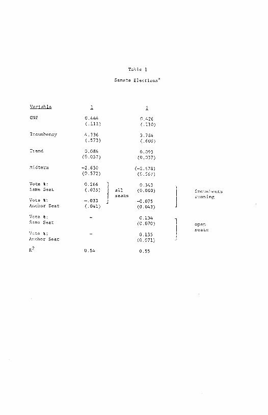
Table 1

Senate Eleotiona*

Variable 1 2

ON'S 0.444 0.426(.111) (.110)

Incumbency 4,336 3.784(.573) (.600)

Trend 0.084 0.093(0.037) (0.037)

Midterm —2,630 (—2.678)(0.572) (0.567)

Vote %: 0.266 ' 0.343Same Seat (.035) all (0.060) incumbents

aeats runningVote %': —.033 —0.075Anchor Seat (.041) (0.043)

Vote %: — 0.134Same Seat (0.070) open

a eatsVote 8: — 0.135

jAnchor Seat (0.071)

R2 0.54 0.55

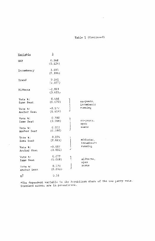
Table I (Continued)

Ljble

CNP 0.368(0.124)

Incumbency 3.693

(0.596)

Trend 0.101(0.037)

Midterm -.2.823

(0.625)

Vote %: 0.446

Same Seat (0.070) on—years,incumbents

Vote %: —0.177 running

Anchor Seat (0.056)

Vote %: 0.200

Same Seat (0.098) on—yeatS.

open

Vote %; 0.092 seats

Anchor Seat (0.098)

Vote %: 0.274

Same Seat (0.065) midtermsincumbents

Vote %: —0.007j

runningAnchor Seat (0.051)

Vote %: 0.077

Same Seat (0.088) midterms

open

Vote %: 0.170 seats

Anchor Seat (0.091)

R2 0,56

*The dependent variable is the Republican share of the two party vote,

Standard errors are in parentheses.

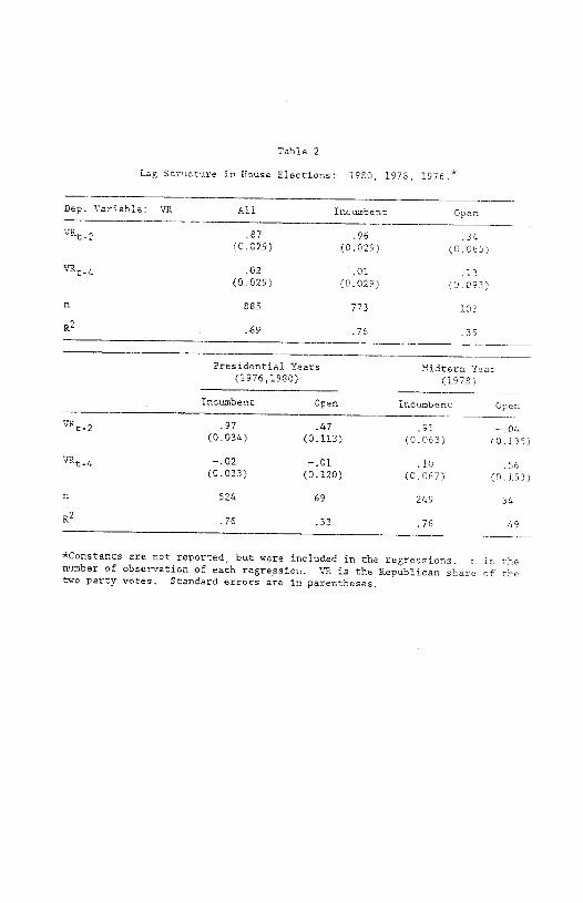
Table 2

Lag Structure in House Eiect6ons: 1980, 1978, 1976.*

Dep. Variable: VR All Incumbent Open

.87 .96 .34(0.029) (0,029) (0.085)

3R4 .02 .01 .13(0.029) (0.029) (0.093)

n 885 773 103

.69 .76 .35

Presidential Years Midterm Year(19761980) (1978)

Incumbent Open Incumbent Open

.97 .47 .91(0.034) (0.113) (0.063) 10.135)

VRt4 —.02 —.01 .10 .56(0.033) (0.120) (0.067) (0,153)

n 524 69 249 34

.76 .33 .76 .49

*Ccnstants are not reported but were included in the regressions. n is thenumber of observation of each regression. YR is the Republican share of thetwo party votes, Standard errors are in parentheses.

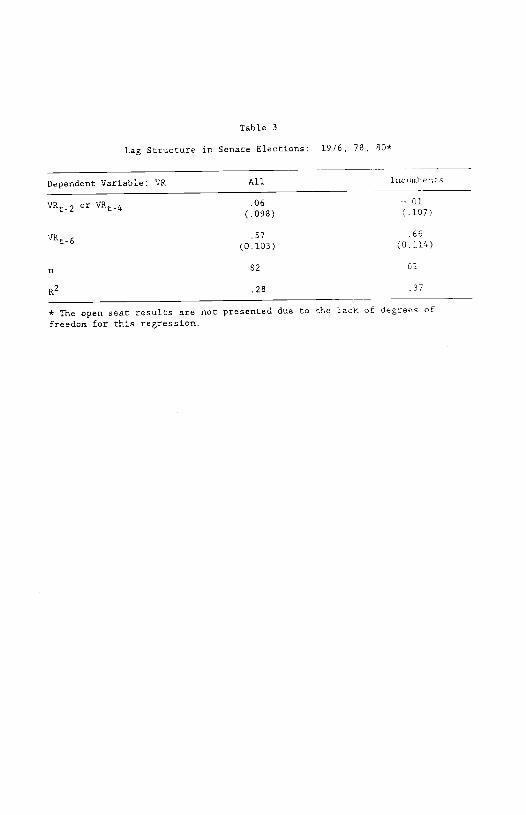
Table 3

Lag Structure in Senate Elections: 1976, 78, 80*

Dependent Variable: VR All IcthflbEtS

VR2 or t-4 .06 01

(.098) (107)

VRt6 57

(0.103)

66(0.114)

n 82 61

R2 .28 .37

* The open seat results are not presented due to the lack of degrees of

freedom for this regression.